dynamic threshold using polynomial surface regression with application to the binarisation of...

8/10/2019 Dynamic threshold using polynomial surface regression with application to the binarisation of fingerprints

http://slidepdf.com/reader/full/dynamic-threshold-using-polynomial-surface-regression-with-application-to-the 1/11

Dynamic threshold using polynomial surface regression with

application to the binarisation of fingerprints

Krzysztof Mielocha , Preda Mihailescub and Axel Munkc

a University of Gottingen, Gottingen, Germany;bUniversity of Paderborn, Paderborn, Germany;c University of Gottingen, Gottingen, Germany

ABSTRACT

Dynamic thresholds are a popular and effective means of binarisation, used in image processing. We show thatthe method is a very special case of a general setting in which input data from a background window are fittedwith a polynomial surface after which the data from a smaller, embedded focus window are thresholded withrespect to the fitted surface.The method has been implemented and used with good results in the context of fingerprint recognition.

Keywords: binarisation, fingerprint, thresholding, polynomial fitting

1. INTRODUCTION

A common model for edge enhancing and thresholding in the context of fingerprint recognition1,2 is inspired bythe study of human visual perception. It consists in gathering context information about contrast and gray valuedistribution from a medium sized background window which contains the focus window which will actually beprocessed. The data in the focus window are thresholded by using the background window information.

The dynamic thresholding method is used for binarising gray level images. The procedure consists in com-puting the average gray value of a square of fixed size surrounding the pixel for each pixel of an image. Thepixel value is then set to black or white, according to whether its initial value was larger then the surroundingaverage or not.

This method may be considered as a two window model in which the inner focus window is reduced to asingle point, which, typically, will be the mean of a given set of values and hence a least squares fit by a constant.One may thus consider the dynamic thresholding as a method in which the data form a background window .These data are fitted by least squares with a constant surface. Within the focus window the gray scale data arebinarised by comparing to the fitting values for the background window.

This analysis of the usual threshold binarisation suggests a natural generalisation:

(i) Replace the fitting constant by a general fitting polynomial surface.

(ii) Let the size of both background and focus window vary.

(iii) Use a sampling step s – thus allowing s > 1 – within the background window, for computing the fittingsurface. This is done for computation economy.

Further author information: (Send correspondence to Krzysztof Mieloch)Krzysztof Mieloch: E-mail: [email protected], Telephone: +49 551 39 13514Preda Mihailescu: E-mail: [email protected], Telephone: +49 5251 60Axel Munk: E-mail: [email protected], Telephone: +49 551 39 13501



In the classical setting described above dynamic threshold binarisation is used in various applications of imageprocessing.3 It is thus likely that the generalisation we present here may be adapted to a wide range of imageprocessing tasks. We developed and optimised it in the context of fingerprint recognition and we will restrictour presentation to this case. Therefore, the bulk of this paper is dedicated in detail to this application. Forthis context we give detailed formulae, pseudocode and visual results of the method. In particular, we show howcareful data management and optimised algorithms can lead to the apparently paradoxical consequence that

surface fitting can be done more efficiently than average value fitting in the classical way. The results of thispart of the paper can thus be used as is by fingerprinting specialists.

2. BINARISATION FOR FINGERPRINT RECOGNITION

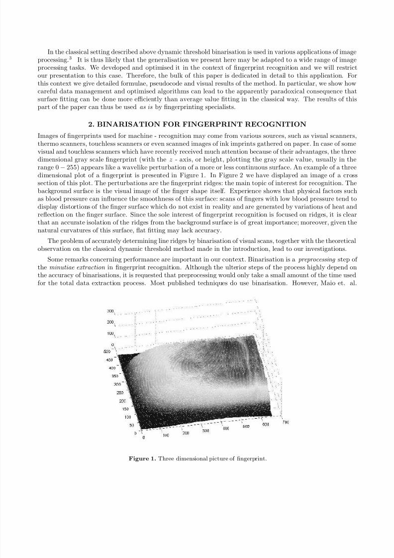
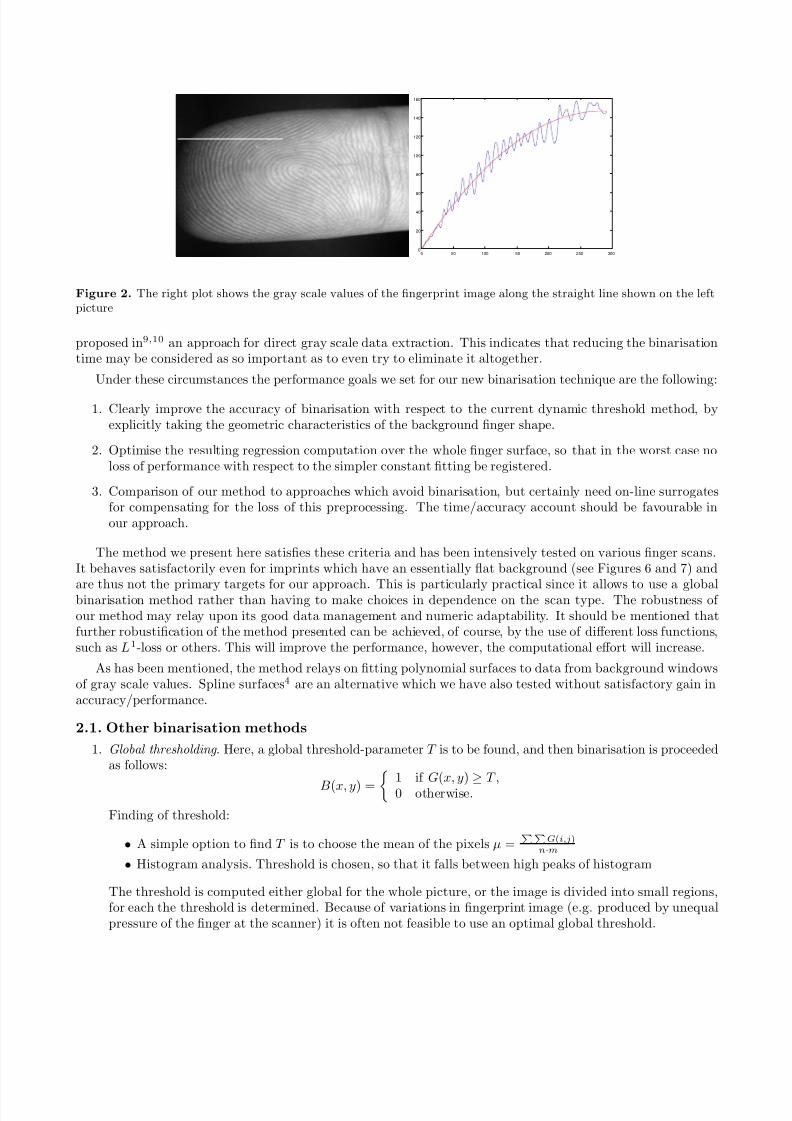
Images of fingerprints used for machine - recognition may come from various sources, such as visual scanners,thermo scanners, touchless scanners or even scanned images of ink imprints gathered on paper. In case of somevisual and touchless scanners which have recently received much attention because of their advantages, the threedimensional gray scale fingerprint (with the z - axis, or height, plotting the gray scale value, usually in therange 0 − 255) appears like a wavelike perturbation of a more or less continuous surface. An example of a threedimensional plot of a fingerprint is presented in Figure 1. In Figure 2 we have displayed an image of a crosssection of this plot. The perturbations are the fingerprint ridges: the main topic of interest for recognition. Thebackground surface is the visual image of the finger shape itself. Experience shows that physical factors suchas blood pressure can influence the smoothness of this surface: scans of fingers with low blood pressure tend todisplay distortions of the finger surface which do not exist in reality and are generated by variations of heat andreflection on the finger surface. Since the sole interest of fingerprint recognition is focused on ridges, it is clearthat an accurate isolation of the ridges from the background surface is of great importance; moreover, given thenatural curvatures of this surface, flat fitting may lack accuracy.

The problem of accurately determining line ridges by binarisation of visual scans, together with the theoreticalobservation on the classical dynamic threshold method made in the introduction, lead to our investigations.

Some remarks concerning performance are important in our context. Binarisation is a preprocessing step of the minutiae extraction in fingerprint recognition. Although the ulterior steps of the process highly depend onthe accuracy of binarisations, it is requested that preprocessing would only take a small amount of the time usedfor the total data extraction process. Most published techniques do use binarisation. However, Maio et. al.

Figure 1. Three dimensional picture of fingerprint.



0 50 100 150 200 250 3000

20

40

60

80

100

120

140

160

Figure 2. The right plot shows the gray scale values of the fingerprint image along the straight line shown on the leftpicture

proposed in9,10 an approach for direct gray scale data extraction. This indicates that reducing the binarisationtime may be considered as so important as to even try to eliminate it altogether.

Under these circumstances the performance goals we set for our new binarisation technique are the following:

1. Clearly improve the accuracy of binarisation with respect to the current dynamic threshold method, byexplicitly taking the geometric characteristics of the background finger shape.

2. Optimise the resulting regression computation over the whole finger surface, so that in the worst case noloss of performance with respect to the simpler constant fitting be registered.

3. Comparison of our method to approaches which avoid binarisation, but certainly need on-line surrogatesfor compensating for the loss of this preprocessing. The time/accuracy account should be favourable inour approach.

The method we present here satisfies these criteria and has been intensively tested on various finger scans.It behaves satisfactorily even for imprints which have an essentially flat background (see Figures 6 and 7) and

are thus not the primary targets for our approach. This is particularly practical since it allows to use a globalbinarisation method rather than having to make choices in dependence on the scan type. The robustness of our method may relay upon its good data management and numeric adaptability. It should be mentioned thatfurther robustification of the method presented can be achieved, of course, by the use of different loss functions,such as L1-loss or others. This will improve the performance, however, the computational effort will increase.

As has been mentioned, the method relays on fitting polynomial surfaces to data from background windowsof gray scale values. Spline surfaces4 are an alternative which we have also tested without satisfactory gain inaccuracy/performance.

2.1. Other binarisation methods

1. Global thresholding . Here, a global threshold-parameter T is to be found, and then binarisation is proceededas follows:

B(x, y) = 1 if G(x, y) ≥ T ,

0 otherwise.

Finding of threshold:

• A simple option to find T is to choose the mean of the pixels µ =PP

G(i,j)n·m

• Histogram analysis. Threshold is chosen, so that it falls between high peaks of histogram

The threshold is computed either global for the whole picture, or the image is divided into small regions,for each the threshold is determined. Because of variations in fingerprint image (e.g. produced by unequalpressure of the finger at the scanner) it is often not feasible to use an optimal global threshold.



background window

b

f oo

focus window

Figure 3. Background and focus windows.

2. Using of the directional field . Here these points indicating ridges one selects the local maximum gray-levelvalues along a direction normal to the local ridge direction.12

3. Using of edge-detector . With use of edge filters, the edges of ridges are found.

3. THE REGRESSION EQUATIONS

Let Γ = {G(x, y) ∈ [0, 255] : 0 ≤ x < W, 0 ≤ y < H } be a gray level image. If n is an odd integer, N n[x, y] isthe neighbourhood of the point x, y consisting of a square of size n, symmetric around (x, y), i.e.

N n[x, y] = {(u, v) ∈ Γ : |u − x| ≤ n − 1

2 and |v − y| ≤

n − 1

2 }. (1)

If (a, b) are the coordinates of a point with respect to the window N n[x, y], its absolute coordinates will thus be(x + a, y + b), or, allowing point addition, (x, y) + (a, b). Note that here we choose the origin of the window in its

centre, thus obtaining negative local coordinates. If one wishes to work in positive integers, one can, for example,situate the origin at the lower left corner of N n[x, y] and add the vector of the centre point as a correction tothe previous formula.

If µn(x, y) =

(u,v)∈N n(x,y)G(u, v)/n2 is the arithmetic mean of the pixel values in the neighbourhood

N n(x, y), dynamic thresholding consists in replacing G(x, y) by the binary value

B(x, y) =

1 if G(x, y) ≥ µn(x, y),0 otherwise.

(2)

Note that hereby the mean µn(x, y) is to be estimated essentially for every single point (x, y). Indeed, the lowaccuracy of the mean value fitting calls for more frequent updates of the threshold µ(x, y).

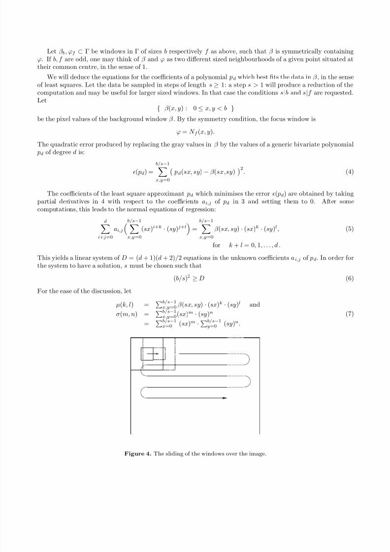
Let b, o and f be positive integers with b = f + 2o: the sizes of a background and a focus window (see

Figure 3); o will be the overlapping width of the background windows while the focus windows of size f slidehorizontally and then vertically over the given image Γ (see Figure 4). Let d be a given degree; the generalbivariate polynomial of degree d may be written as:

pd(x, y) =d

i+j=0

ai,j · xiyj ; (3)

note that the sum of the powers of x and y (the weight of pd(x, y)) is bounded by d.



Let β b, ϕf ⊂ Γ be windows in Γ of sizes b respectively f as above, such that β is symmetrically containingϕ. If b, f are odd, one may think of β and ϕ as two different sized neighbourhoods of a given point situated attheir common centre, in the sense of 1.

We will deduce the equations for the coefficients of a polynomial pd which best fits the data in β , in the senseof least squares. Let the data be sampled in steps of length s ≥ 1: a step s > 1 will produce a reduction of thecomputation and may be useful for larger sized windows. In that case the conditions s|b and s|f are requested.Let

{ β (x, y) : 0 ≤ x, y < b }

be the pixel values of the background window β . By the symmetry condition, the focus window is

ϕ = N f (x, y).

The quadratic error produced by replacing the gray values in β by the values of a generic bivariate polynomial pd of degree d is:

( pd) =

b/s−1x,y=0

pd(sx, sy) − β (sx,sy)

2. (4)

The coefficients of the least square approximant pd which minimises the error ( pd) are obtained by takingpartial derivatives in 4 with respect to the coefficients ai,j of pd in 3 and setting them to 0. After somecomputations, this leads to the normal equations of regression:

di+j=0

ai,jb/s−1x,y=0

(sx)i+k · (sy)j+l

=

b/s−1x,y=0

β (sx, sy) · (sx)k · (sy)l, (5)

for k + l = 0, 1, . . . , d .

This yields a linear system of D = (d + 1)(d + 2)/2 equations in the unknown coefficients ai,j of pd. In order forthe system to have a solution, s must be chosen such that

(b/s)2 ≥ D (6)

For the ease of the discussion, let

µ(k, l) = b/s−1

x,y=0 β (sx, sy) · (sx)k · (sy)l and

σ(m, n) = b/s−1

x,y=0(sx)m · (sy)n

= b/s−1

x=0 (sx)m ·b/s−1

y=0 (sy)n.

(7)

Figure 4. The sliding of the windows over the image.



Let us also define the following operations on ordered pairs of integers:

(i, j) + (k, l) := (i + j, k + l) and

ι−1(m, n) := (m + n)(m + n + 1)

2 + m.

Note that hereby, ι−1

: N2

→ N is a bijective counting of pairs of integers; it is thus indeed the inverse of abijective map ι : N → N

2. We shall use this map for enumerating the pairs (i, j) : i + j ≤ d in terms of a singleinteger n ≤ D: thus we have

∀ n ≤ D : ι(n) = (i, j) with i + j ≤ d.

This notation simply brings in evidence the fact that our linear system with double indexed unknowns a i,j is infact a simple linear system in D unknowns, which is transformed into a system with double indexed unknownsby using ι. With these prerequisites, the system 5 may be written as

di+j=0

ai,j · σ(i + k, j + l) = µ(k, l), for k + l = 0, 1, . . . , d.

This can be rewritten in terms of matrices as

A(d) · a = M, (8)

with

A(d)m,n = σ

ι(m) + ι(n)

,an = aι(n), andMn = µ

ι(n)

, for m, n = 0, 1, . . . , D − 1.

(9)

The dynamical threshold method with polynomial regression consists in the following:

I. Fix the parameters b, f,s and d. Note that o = b − 2f is herewith fixed, too.

II. Position the background window: start in a corner of the image and slide this background in horizontaland then vertical directions along the image.

III. For each position of the background window β (x, y), compute the corresponding regression polynomial pd = pd[x, y].

IV. For each point (a, b) in the focus window ϕ(x, y), estimate the polynomial pd[x, y] at (a, b) and comparethe image data G(a + x, b + y) with the the predicted values pd[x, y](a, b), like in 2.

V. Reposition the background window by shifting in steps of f , horizontally and vertically, until reaching thediametral corner to the starting one. For each new position repeat III. and IV.

4. DATA MANAGEMENT

It is essential to avoid repetition of identical operations in order to reduce the computation cost. We shallconcentrate in this section on some procedures for optimising the performance.

First, note that the matrix A(d) does not depend upon the image data or the position of the backgroundwindow 7, 8. In fact, it only depends upon the size parameters b and s and the degree d. For fixed b, s it alsohas the nice inheritance property consisting in the fact the A(d) ⊂ A(d) for d < d, in the sense that A(d) isthe submatrix of size (d + 1)(d + 2)/2 of A(d) situated in its upper left corner.

Since the system 8 needs to be solved for each position of the background window, factoring the matrix A(d)in its L · U decomposition5 before running the algorithm will reduce the system solving times form O(D3) toO(D2) operations. Since all the entries of A are essentially products of sums of different powers of the integers



< (b/s), the matrix can be factorised in its general shape using symbolic computation. This we have done usingthe PARI11 package for degrees d < 9 and it has the effect of allowing integer arithmetic instead of floating point: the common denominators of the divisors involved in the solution of 8 have nice algebraic closed shapes.

The right hand side of 8 carries the image data and global precomputations are thus not possible. It ishowever possible and important to take overlaps in consideration for minimising the update costs for the dataµ(x, y). Since the background window is shifted only by the size f of the focus window at each step, a certainamount of data will contribute to the values µ(k, l) for more than one window. We use a procedure which consistsin adding separately the column data and then accumulating them to produce the window data in µ(k, l). Letus thus define

Y l(x, y) =

b/s−1i=0

(s · i)l · G(x, y + i · s),

and

µx,y(k, l) =

b/s−1i,j=0

G(x + is,y + js) · (si)k · (sj)l

=

b/s−1

i=0 (si)

k

· Y l(x + is,y). (10)

For fixed y, the values Y l(x, y) will be computed only once and then be used for computing all µx,y(k, l) withthat given y − value. At a horizontal shift, only f /s new Y − values will replace the first f /s values involved inthe current µx,y(k, l) sums; similarly, at a vertical shift, only f /s new G(x, y) values will replace the first ones ina Y - sum. We shall split these operation in a sequence of f /s steps, which consist in replacing a starting valueby a new value in a given sum. The following lemma formalises the situation:

Lemma 4.1. Let V = { v(n) ∈ N : n = 0, 1, . . . N } a set of data, b,s,k > 0 integer parameters such that s2 << N and consider the following evaluations on the set V :

E k(u) =

b/s−1

i=0

(is)k · v(u + is),

and the differences ∆(E k(u)) = E k(u + s) − E k(u).

Then the followings recursion holds:

(i) ∆(E 0(u)) = v(u + b) − v(u),

(ii) ∆(E k(u)) = bk · v(u + b) −k−1

i=0

ik

sk−iE i(u + s).

Proof . Item (i) is a direct computation: E (u+s)−E (u) = b/s

i=1 v(u+is)−b/s−1

i=0 v(u+is) = v(u+b)−v(u).Item (ii) follows after some careful regrouping of terms in the equality.

All the recursive computations needed for the updating of the values µ(x, y) when the background windowslides along the gray value image are obtained by applying the above lemma for various choices of V . We firstapply the lemma to the vertical shift. In this case v(y) = G(x, y), for fixed x and E l(y) = Y l(x, y). Lemma 4.1provides the values of the step shifts when y is increased by s.

For the horizontal shift, consider the data v(x) = Y l(x, y), for fixed l and y . The lemma provides us the stepchanges µx+s,y(k, l) − µx,y(k, l) for the fixed l . It will thus have to be applied for d different values of l, in orderto update all the µ - values in the right term of 8. After computing the current fitting polynomial pd[x, y], thebinarisation requires its evaluation at all the points within the small focus window. Here again operation can bespared by adequate finite difference operations. We leave it to the reader to develop his preferred algorithm forthis small substep.



We have so far gathered the informations for an algorithm for dynamic thresholding with polynomial surfaceregression. We express this algorithm below in detail, using pseudocode description. The input of the algorithmis the following:

INPUT:

1. A gray value image G

= {G(x, y) : 0 ≤ x < W ; 0 ≤ y < H ; 0 ≤ G(x, y) < 256}.2. The auxiliary parameters b, f which are the (odd) sizes of the background and the focus windows, respec-

tively. The overlap is o = (b − f )/2 and at each step the background window is shifted by o horizontallyor vertically.

3. The sampling step s ≥ 1 and the degree of the fitting polynomial d ≥ 0. Note that for d = 0 we have theclassical dynamic threshold method, with an improved data management.

The output is a binary image B = B(x, y) of the same size as the gray scale image.

For the linear algebra steps for L-U decomposition and solution of the linear system 8 any standard solutioncan be used.

5. PRACTICAL EXPERIENCE

The procedure described above has been used on a large scale of fingerprint images obtained by a touchlessdevice with various scan qualities (for example see figure 5). The approach is considered to perform better if forcomparable run times (for dynamic moments this implies an adequate choice of the degree and sampling step,such as to keep the pace with the simpler average estimate) the resulting binarisation is more accurate. We havenot develop an abstract accuracy metric; rather the accuracy is evaluated both visually and by integration inour own minutiae extraction algorithm. The dynamic threshold method has found to perform overall better, inparticular in images of less quality, where it could extract more contrast.

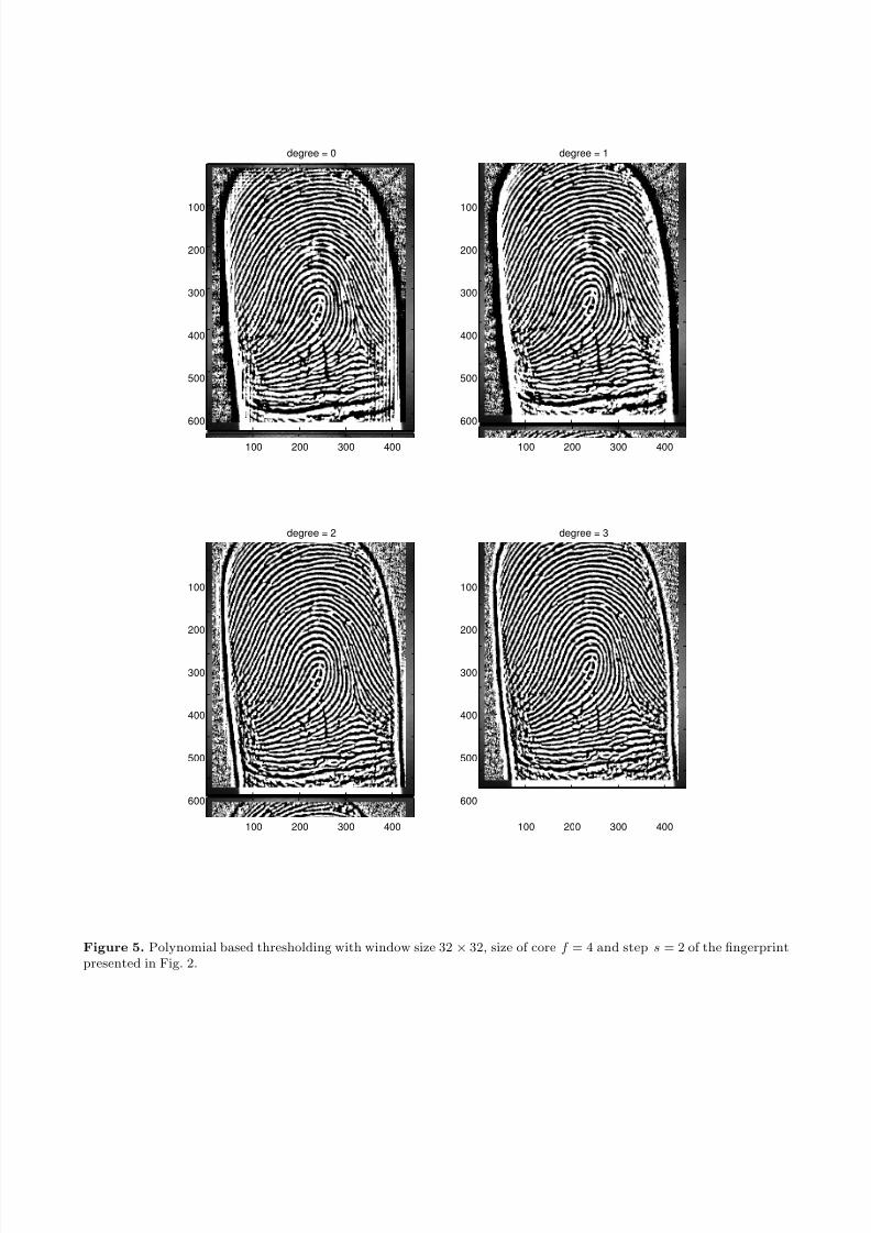
In fig. 5 we can observe that significant improvement of the binarisation quality when the degree changes itsvalue from 0 to 1 and from 1 to 2, whereas there is hardly improvement of quality when increasing the degree of polynomial from 2 to 3. Indeed, in our experiments the degree of 2 has been found to be sufficient.

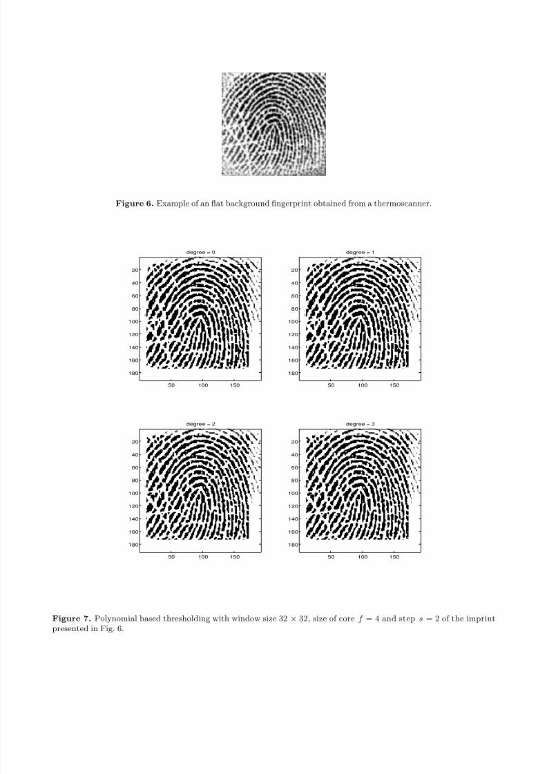
The tests for ”flat” fingerprint images (example - fig. 6) has shown there is no improvement by increasing thedegree value (fig. 7). This implies, the polynomial based thresholding works for this type of fingerprint imagesas good as the standard mean thresholding.

REFERENCES

1. D. Maltoni, D. Maio, A. K. Jain, and S. Prabhakar: Handbook of Fingerprint Recognition , Springer Verlag,June 2003.

2. A. K. Jain and S. Pankanti: ”Automated Fingerprint Identification and Imaging Systems”, Advances inFingerprint Technology, 2nd Ed. (H. C. Lee and R. E. Gaensslen), CRC Press, 2001.

3. B. Jahne: ”Digital Image Processing”, Sprinter Verlag, 2002

4. P. Diercks: Curve and Surface Fitting with Splines , Monographs on Numerical Analysis, Oxford UniversityPress (1995)

5. G. H. Golub and Ch. van Loan: Matrix Computations . The Johns Hopkins University Press, Baltimore, 1983.

6. L. Hong, Y.Wan and A.K. Jain: ” Fingerprint Image Enhancement: Algorithms and Performance Evalua-tion”, Proc. IEEE Comp. Soc. Workshop on Empirical Evaluation Techniques in Computer Vision, SantaBarbara. June 1998, pp. 117-134.

7. L. Hong, Y. Wan and A.K. Jain: ”Fingerprint Image Enhancement: Algorithms and Performance Evalua-tion”, IEEE Transactions on PAMI ,Vol. 20, No. 8, pp.777-789, August 1998.

8. L. Hong, A.K. Jain, S. Pankanti and R. Bolle: ”Fingerprint Enhancement”, Proc. IEEE Workshop onApplications of Computer Vision, Sarasota, Fl, pg. 202-207, Dec. 1996.



degree = 0

100 200 300 400

100

200

300

400

500

600

degree = 1

100 200 300 400

100

200

300

400

500

600

degree = 2

100 200 300 400

100

200

300

400

500

600

degree = 3

100 200 300 400

100

200

300

400

500

600

Figure 5. Polynomial based thresholding with window size 32 × 32, size of core f = 4 and step s = 2 of the fingerprintpresented in Fig. 2.



Figure 6. Example of an flat background fingerprint obtained from a thermoscanner.

degree = 0

50 100 150

20

40

60

80

100

120

140

160

180

degree = 1

50 100 150

20

40

60

80

100

120

140

160

180

degree = 2

50 100 150

20

40

60

80

100

120

140

160

180

degree = 3

50 100 150

20

40

60

80

100

120

140

160

180

Figure 7. Polynomial based thresholding with window size 32 × 32, size of core f = 4 and step s = 2 of the imprintpresented in Fig. 6.



9. D. Maio and D. Maltoni: ”Direct Gray-Scale Minutiae Detection in Fingerprints”, IEEE Transactions onPattern Analysis Machine Intelligence, vol.19, no.1, pp.27-40, 1997.

10. D. Maio and D. Maltoni: ”Minutiae extraction and filtering from gray-scale images”, in L.C. Jain, U. Halici,I. Hayashi, S.B. Lee, Intelligent Biometric Techniques in Fingerprint and Face Recognition, CRC Press, 1999.

11. H. Cohen et. num. al.: PARI/GP, Laboratoire A2X , http://pari.math.u-bordeaux.fr

12. R. Bolle, A. Senior, N. Ratha and S. Pankanti: ”Fingerprint Minutiae: A Constructive Definition”, LectureNotes in Computer Science, Vol. 2359/2002, p. 58–66

dynamic threshold using polynomial surface regression with application to the binarisation of...

Documents