dynamic stability of time-delayed feedback control system ... · dynamic stability of time-delayed...

Dynamic stability of Time-Delayed Feedback Control System by FFT

based IHB Method

R. K. MITRA

Department of Mechanical Engineering

National Institute of Technology, Durgapur (Deemed University)

West Bengal, Pin-713209

INDIA

[email protected], http://www.nitdgp.ac.in/faculty_details.php?id=122

A. K. BANIK

Department of Civil Engineering

National Institute of Technology, Durgapur (Deemed University)


INDIA

[email protected], http://www.nitdgp.ac.in/faculty_details.php?id=21

S. CHATTERJEE

Department of Mechanical Engineering

Bengal Engineering and Science University, Shibpur


INDIA

[email protected], http://www.becs.ac.in/aboutshyamal-chatterjee-mech-menuitem

Abstract: - The forced Duffing oscillator is investigated by intentional time-delayed displacement

feedback by fast Fourier transform based incremental harmonic balance method along with

continuation technique (FFT-IHBC). FFT-IHBC can efficiently develop frequency response curves

with all stable and unstable solutions and solution branches. Appreciable reduction in peak value of

response and gradual reduction in the skew-ness in frequency response curve is observed with the

introduction of gain and delay. Further, frequency response curves with all stable solutions can be

achieved with appropriate choice of gain and delay in the primary and secondary stability zones of

linear stability analysis. The results obtained by this method are compared with numerical integration

method and they match perfectly.

Key-Words: - Fast Fourier transform; incremental harmonic balance method; are length continuation;

intentional time-delayed feedback; Floquet stability.

1 Introduction

Controlling resonant vibrations of flexible machine

components and structural members has always

been an important area of research for engineers. In

the past various methods analytical, semi-analytical

and numerical methods were available for

controlling resonant vibrations. Though active

vibration control is a superior to passive control

techniques, presence of unavoidable time delays in

the feedback circuit seriously limits the performance

of an active control system and in the worst case the

system response may even become unbounded.

Thus, it is extremely difficult to meet the desire

objectives of vibration control systems under the

presence of uncontrollable time-delay. The common

mathematical methods available for the analysis of

the aforesaid class of systems is the method of

Multiple Time Scales (MTS) and straight forward

harmonic balance (HB) analysis. But such methods

works well only for weakly non-linear systems and

for time-delays smaller compared to the natural time

period of vibration of the system. A comprehensive

survey of the recent research on the field is available

in [1].

Olgac et al. [2, 3] have developed an active

vibration absorber based on linear time-delayed

WSEAS TRANSACTIONS on APPLIED and THEORETICAL MECHANICS R. K. Mitra, A. K. Banik, S. Chatterjee

E-ISSN: 2224-3429 292 Issue 4, Volume 8, October 2013

state feedback, which they have termed as the

delayed resonator. Hu et al. [4] have reported time-

delayed state feedback control of the primary and

1/3 sub-harmonic resonances of a forced Duffing

oscillator. Udwadia et al. [5 to 7] have investigated

the application of time-delayed velocity feedback

for controlling the vibrations of structural systems

under seismic loading. Maccari [8] and Atay [9]

have studied vibration control of self-excited

systems. The primary resonance of a cantilever

beam under the time-delayed feedback control has

been studied by Maccari [10]. Chatterjee [11] have

discussed time-delayed feedback control of various

friction-induced instabilities. Vibration control by

recursive time-delayed acceleration feedback has

also been studied by Chatterjee [12]. Ram et al. [13]

consider the eigenvalue assignment problem for a

linear vibratory system using state feedback control

in the presence of time-delay. El-Bassiouny and El-

kholy [14] present analytical and numerical studies

on the effect of time-delayed feedback of a non-

linear SDOF system under external and parametric

excitations.

As stated earlier, presence of unavoidable

time delays in the feedback circuit seriously limits

the performance of an active control system by

destabilizing it at high control gains. In order to

circumvent this undesirable situation, time-delay is

intentionally introduced in the feedback path where,

the gain and the time-delay are both controllable.

Further, literature survey reveals that studies on the

effect of intentional time-delayed feedback for such

class of resultant nonlinear system are scarce (to the

best of the authors’ knowledge and information).

The present study is therefore motivated by the need

for a better semi-analytical prediction of complex

periodic via fast Fourier transform based

incremental harmonic balance method along with a

continuation technique (IHB-FFTC). Since the

system or the feedback control law (which will be

developed and introduced in the feedback path) is

strongly non-linear, the efficiency of the method to

study the response and stability of such system is

attempted. The stability of the periodic solution is

examined by Floquet theory. The results show that

the response curve can be suppressed to the desired

level with appropriate choice of delay and gain

parameters.

2 Fast Fourier Transform Based

Incremental Harmonic Balance

Method for Time-Delayed Feedback

Systems

2.1 Fourier discretization Consider the set of non-linear ordinary deferential

equations for a multi degree of freedom dynamical

system with time-delay of the following general

form

0),,,,,,,()( tdfxxxxt d (1)

With the periodic conditions

)2()( and

),2()( ),2()(

htxtx

htxtxhtxtx

(2)

In this vector equation, is analytic, x(t) is the

unknown response of the non-linear system, or in

general, the dependent variable vector, )(txd is the

time-delayed function, is the non-dimensional

excitation frequency, d is the time-delay, and f is the

external harmonic excitation amplitude. Over dots

denote derivatives with respect to the non-

dimensional time t and h is the integer order of the

sub-harmonic response being considered.

The first step of the IHB method is the Newton–

Raphson iterative procedure. To obtain a periodic

solution of Eq. (1) one needs to guess a solution at

the beginning of the procedure which may be taken

as the solution of linear system. A neighboring

solution can be expressed by adding the

corresponding increments (symbolized by ) to

them as follows,

fff

xxxxxx ddd

and

, , ,

(3)

Thus, the left side variables of Eq. (3) can be

regarded as the neighbouring states while that on the

right side as the sum of known states and their

increments. Substituting Eq. (3) into Eq. (1) one

obtains the following incremental equation:

0),,,

,,,,()(

tdff

xxxxxxxxt dd

(4)

Now expanding Eq. (4) by Taylor’s series about the

initial state up to the first order, the linearized

incremental equations are obtained as,

0)(

tff

xx

xx

xx

xx

d

d

(5)

Here )(t is the residue or corrective term which

will vanish when the solution is exact. Now replace

Ff

W

Dx

Kx

Cx

Mx d

and

, , , ,

(6)

With these, Eq. (5) takes the form



dxDxKxCxM

0)( tfFW (7)

The terms FWDKCM and , , , , can in general be

time (t) varying and are called the equivalent

incremental mass, damping, stiffness, delay,

frequency and excitation respectively. Eq. (5) or (7)

represents a set of linear, second order, variable

coefficient, ordinary differential equations (ODEs).

The second step of the IHB method is to expand the

generalized coordinate x(t) and the corresponding

increment )(tx into Fourier series for periodic

response.

0

0

2

1

)(

)(

a

a

tx

tx

1

sincosi i

i

i

i

h

it

b

b

h

it

a

a (8a)

AY

YA

)(

)(

tx

tx, (8b)

where i denotes any positive integer and

. . . cos . . .

2cos cos 1

h

it

h

t

h

tY

. . . sin . . .

2sin sin

h

it

h

t

h

t (8c)

Or ] 1 [ ii scY , (8d)

where

h

itci cos and

h

itsi sin

. . . . . . . . . . . .

2i21i21

0 bbbaaaa

A (8e)

and

. . . . . .

2i21

0 aaaa

A

T

i21i . . . . . . . . . bbbb (8f)

Here, the upper subscript symbol ‘T’ denotes the

transpose of a matrix. These solutions include all

harmonics up to a certain order n and have sub-

harmonic order h. From now on it is assumed that

)(tx is an approximately known solution and )(tx

is to be found such that )()( txtx is a new

solution. Therefore all functions of time in (6) are

known for given )(tx and they can be correlated by

expanding using Fourier series as follows:

2

1

)(

)(

0

0

C

M

tC

tM

1

sin cos u

su

su

cu

cu

h

ut

C

M

h

ut

C

M (9a)

2

1

)(

)(

0

0

D

K

tD

tK

1

sin cos u

su

su

cu

cu

h

ut

D

K

h

ut

D

K, (9b)

and

2

1

)(

)(

)(

0

0

0

F

W

t

tF

tW

1

sin cos u s

u

su

su

cu

cu

cu

h

utF

W

h

utF

W

(9c)

Now, the Fourier coefficients of these functions can

be calculated most efficiently by applying FFT (fast

Fourier transform) algorithm. Considering xd as the

time-delayed displacement of the form

)()( dtxtxd , the Fourier series of dx and

dx are expressed as:

0

0

2

1

)(

)(

a

a

dtx

dtx

h

ωd-ti

b

b

h

ωd-ti

a

a

i

i

i i

i )(sin

)(cos

1

(10)

Substituting Eq. (8a), (9) and (10) into Eq. (5), we

obtain the following linear matrix equation for the

unknown increment }{ A ,

}{ }]{[)}({ WADKCMY t

0}ΦF {}{ }{ f (11a)

Where,

. . . W . . . W W /2W cu

c2

c10W

T . . . W . . . W W s

us

2s

1 , (11b)

and

. . . F . . . F F /2F cu

c2

c10 [F

T] . . . F . . . F F su

s2

s1 (11c)

Let us define ][][ DKCMJ as the Jacobian

(gradient or tangential) matrix with respect to }{ A

in which the matrices ][M , ][C , ][K and ][D are

defined by as

,)(]][[)( xtMt AMY (12a)

,)(]][[)( xtCt ACY (12b)

,)(]][[)( xtKt AKY (12c)

and

)()(]][[)( dtxtDt ADY (12d)



2.2 Evaluation of Jacobian matrix

The elements of the Jacobian matrix in Eq. (12) are

effectively calculated using FFT method. Here we

will evaluate only ][D in detail. The results for ][C ,

][K and ][M are supplied directly from Leung and

Chui (1995), [15].The elements of ][D in terms of

Fourier components of D (t) are expressed as,

][

0

0

0000

ssij

scij

si

csij

ccij

ci

sj

cj

DDD

DDD

DDD

D (13)

From Eq. (12d),

i

i

ssij

scij

si

csij

ccij

ci

sj

cj

ii

a

a

a

DDD

DDD

DDD

sc

0

0

0

0000

] 1 [

1

0

2 u

usuu

cu sDcD

D

1

0 sin cos 2

j

jjjh

djs

h

djca

a

h

djc

h

djsb jj

sin cos j (14)

where 0D , cuD and s

uD are the Fourier coefficients

of )(tD .

(i).Equating first the coefficients of 0a on both side

of Eq. (14), we obtain,

1

0

0

0

00

22

1 ] 1 [

u

usuu

cu

si

ciii sDcD

D

D

D

D

sc (15)

This implies,

si

si

ci

ci DDDDDD

2

1 and ,

2

1 ,

4

100000

(ii) Next, evaluate the coefficient of ja on both

sides of Eq. (14) for a certain j.

1

0

0

2 ] 1 [

u

usuu

cu

scij

ccij

cj

ii sDcDD

D

D

D

sc

h

djs

h

djc jj

sin cos (16a)

scij

ccij

cj

ii

D

D

D

sc

0

] 1 [

j

u

usuu

cu csDcD

D

h

dj

1

0

2cos

j

u

usuu

cu ssDcD

D

h

dj

1

0

2sin

(16b)

Next, we apply Galerkin's method or the harmonic

balance method to evaluate the Fourier coefficients.

Multiplying both sides of the above equation by ci

and si, respectively and integrating over time t from

zero to h2 and then equate it to zero, we have

respectively,

dt

D

D

D

scc

h

scij

ccij

cj

iii ] 1 [

2

0

0

dtccsDcDD

h

djji

h

u

usuu

cu

2cos

2

0 1

0

dtscsDcDD

h

djji

h

u

usuu

cu

2sin

2

0 1

0

,

(17)

and

dt

D

D

D

scs

h

scij

ccij

cj

iii ] 1 [

2

0

0

dtcssDcDD

hdj ji

h

u

usuu

cu

2)/cos(

2

0 1

0

dtsssDcDD

hdj ji

h

u

usuu

cu

2)/sin(

2

0 1

0

(18)

Use of the following general trigonometric relations

and orthogonality relations between sine and cosine

functions are helpful to simplify Eq. (17) and (18).

Here q and r are zero or integers.

rqrqrq sscs 2

1 (19a)

rqrqrq cccc 2

1 (19b)

rqrqrq ccss 2

1 (19c)

rqdtcs

h

rq and allfor 0

2

0

(19d)



for 0

for

2

0

rq

rqhdtss

h

rq

(19e)

for 0

for

for 2

2

0

rq

0rqh

0rq hπ

dtcc

h

rq

(19f)

Therefore, for the cosine terms we have,

h

u

usuu

cu

ccij sDcD

D

h

djDh

2

0 1

0

2cosπ

dtcc jiji )(2

1

2

)/sin(

2

0 1

0

h

u

usuu

cu sDcD

Dhdj

dtss jiji )(2

1

(20)

A similar expression can be obtained for sine terms

and not shown to maintain brevity. Finally, from Eq.

(17) and (18) we obtain,

0for sin2

1 cos

2

1 0

iD

h

djD

h

djD s

ici

cj

(21a)

cji

ccij D

h

djD ||

cjiDcos

2

1

0for )sgn(cos ||

iDjiD

h

dj sji

sji

(21b)

sji

sji

scij DjiD

h

dj

h

djD ||)sgn(cos

2

1

iDh

dj cji allfor Dsin c

ji||

(21c)

(iii) Next we equate the coefficient ofjb on both

sides of Eq. (14) for a certain j.

1

0

0

2 ] 1 [

u

usuu

cu

ssij

csij

sj

ii sDcDD

D

D

D

sc

h

jωωc

h

jωωs jj sin cos (22a)

ssij

csij

sj

ii

D

D

D

sc

0

] 1 [

j

u

usuu

cu ssDcD

D

h

dj

1

0

2cos

j

u

usuu

cu csDcD

D

h

dj

1

0

2sin

(22b)

Applying the harmonic balance method as above we

obtain,

c

jsj

sj D

h

djD

h

djD

sin cos

2

1 0 (23a)

sji

sji

csij DjiD

h

djD ||)sgn(cos

2

1

sin ||

cji

cji DD

h

dj, (23b)

and

cos

2

1 ||

cji

cji

ssij DD

h

djD

s|j-i|D)j-isgn(sin s

jiDh

dj (23c)

The elements of ][M in terms of Fourier

components of M(t) are expressed as,

][

0

0

0000

ssij

scij

si

csij

ccij

ci

sj

cj

MMM

MMM

MMM

M , (24)

where,

00000 si

ci MMM , (25a)

cj

cj M

h

jM

2

2

02

, (25b)

cji

cji

ccij MM

h

jM ||2

2

2

, (25c)

0for )sgn(2

||2

2

iMjiM

h

jM s

jic

jiscij

,

(25d)

Mh

jM s

js

j

2

2

02

, (25e)

sji

sji

csij MjiM

h

jM ||2

2

)sgn(2

, (25f)

and

0for 2

2

2

iMM

h

jM c

jic

|j-i|ssij

(25g)

The elements of ][C in terms of Fourier

components of C(t) are expressed as,



ssij

scij

si

csij

ccij

ci

sj

cj

CCC

CCC

CCC

0

0

0000

][C , (26)

where,

00000 si

ci CCC , (27a)

0iCh

jC s

jc

j for 2

0, (27b)

0iCjiCh

C sji

sji

ccij for )sgn(

2

1 ||

, (27c)

iCCh

C cji

cj-i

scij allfor

2

1 || , (27d)

2

0cj

sj C

h

jC , (27e)

cji

cji

csij CC

hC ||

2

1 , (27f)

and

0for )sgn(2

1 || iCjiC

hC s

jis

jissij . (27g)

The elements of ][K in terms of Fourier

components of K(t) are expressed as,

ssij

scij

si

csij

ccij

ci

sj

cj

KKK

KKK

KKK

0

0

0000

][K (28)

Wheresi

si

ci

ci KKKKKK

2

1 ,

2

1 ,

4

100000 ,

cj0 K

2

1 c

jK , K2

1 ||

cji

cji

ccij KK

0for )sgn(K2

1 ||

sji iKjiK s

jiscij ,

KK sj

sj

2

1 0 , s

jis

jicsij KjiKK ||)sgn(

2

1 ,

and 0for K2

1 c

|j-i| iKK cji

ssij

Next }{W , }{F and }{Φ in Eq. (11a) are calculated

using FFT algorithm and it is solved for the

unknown coefficient vector A .

Finally, the matrix Eq. (11a) is solved at

each time step using the Newton-Rapson iterative

process.

2.3 Path following and parametric

continuation The FFT-IHB method with a variable parameter is

ideally suited to parametric continuation for

obtaining the response diagrams of nonlinear

systems. After obtaining the solution for the

particular value of a parameter, the solution for a

new parameter slightly perturbed from the old one

can be obtained by iterations using the previous

solution as an approximation. The main aim of the

path following and parametric continuation is to

effectively trace the bifurcation sequence as a

parameter of the system is varied. In this study, an

arc length procedure16

is adopted for the parametric

continuation.

Introducing the path parameter, the

augmenting equation for a general system can be

written as:

0)( X (29)

where T],}[{}{ T AX . A good choice of the

function }X{g is {X}X}XTg {)( . Considering the

increments in }{A , F and , the incremental

equation is obtained as

0}{T

A

A (30)

Together with (11), we obtain the augmented

incremented incremental equation

}{ }]{[)}({ WADKCMY t

}{ }{ }{ }{ 0ΦFΦ f (31)

--

ΦA

A

WJ

XJ X

T

][

}]{[ (32)

where ][][ DKCMJ as before, and ][ XJ is

the Jacobian matrix which is modified with respect

to {X}. Considering the portion of the equilibrium

path of the solution branch, the augmenting equation

can be written as

0}{}{)( cXXX'XT (33)

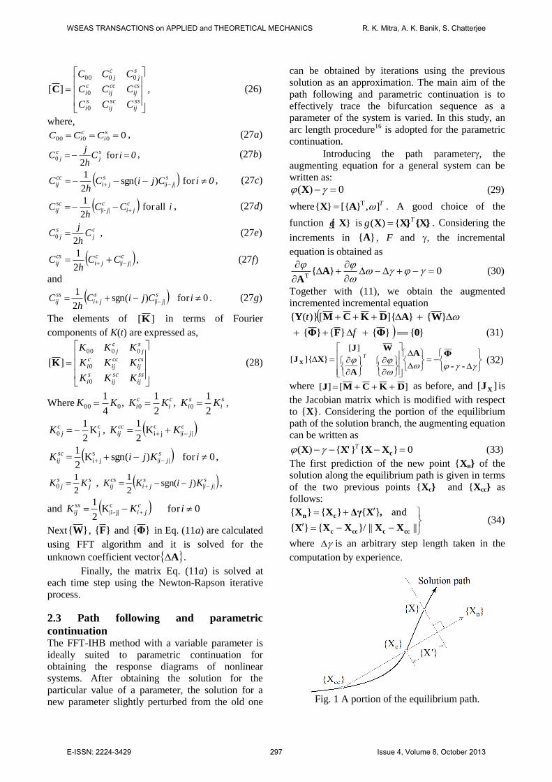
The first prediction of the new point {Xn} of the

solution along the equilibrium path is given in terms

of the two previous points {Xc} and {Xcc} as

follows:

||||}/{}{

and}{}{}{

cccccc

cn

XXXXX

,XΔγXX (34)

where is an arbitrary step length taken in the

computation by experience.

Fig. 1 A portion of the equilibrium path.



2.4 Stability analysis of periodic solutions

When the steady-state solution for time-delay

system is computed by using the FFT-IHBC

method, the stability of the periodic (or almost

periodic) solution is checked by means of Floquet

theory for two important reasons. First, stable

branches can be distinguished from unstable ones

and bifurcation points can be located by monitoring

eigenvalues of the monodromy matrix. In this paper

Floquet theory is modified to analyse the stability of

the periodic solution of time-delayed displacement

feedback system. This is done by perturbing the

state variables about the steady-state solution, which

results in a system of linearized equations with

periodically varying coefficients. The perturbed

equation of motion is always autonomous. When the

solution is perturbed by }{ x , the incremental linear

matrix ordinary differential equation is

0}{}{}{}{ dxDxKxCxM (35)

In state space form Eq. (30) can be written as

}{

}{

M

C

1

1 0

}{

}{

x

x

x

xDK

Mx

x

dt

dd

(36)

}]{)([}{ ztz B (37)

Where the transition matrix [B] is periodic with tine

period T, i.e. [B(t)]=[B(t+T )]. The stability of Eq.

(32) is checked by evaluating the eigenvalues of the

monodromy matrix [Z], which transforms the state

vector {zn} at t=nT to {zn+1} at t=(n + 1)T. If the

absolute magnitudes of the eigenvalues are less than

unity, the solution is stable. If at least one of the

eigenvalues has a magnitude greater than one, then

the periodic solution is unstable. The way the

eigenvalues leave the unit circle determines the

nature of bifurcations. The explicit form of [Z] can

be written as [17],

)]([exp][1

titn

i

BZ (38)

where ,/ NTt and N represents the number of

divisions used to divide one period T. The efficient

numerical evaluation ][Z is achieved by making use

of the definition of the matrix exponential

!

][...

!2

][][][][exp

2

n

tttt

nBB

BIB

(39)

where [I] is the identity matrix. For small time

intervals 0t , the series in equation converges

rapidly, and the value of the matrix exponential can

be accurately approximated by a finite number of

terms.

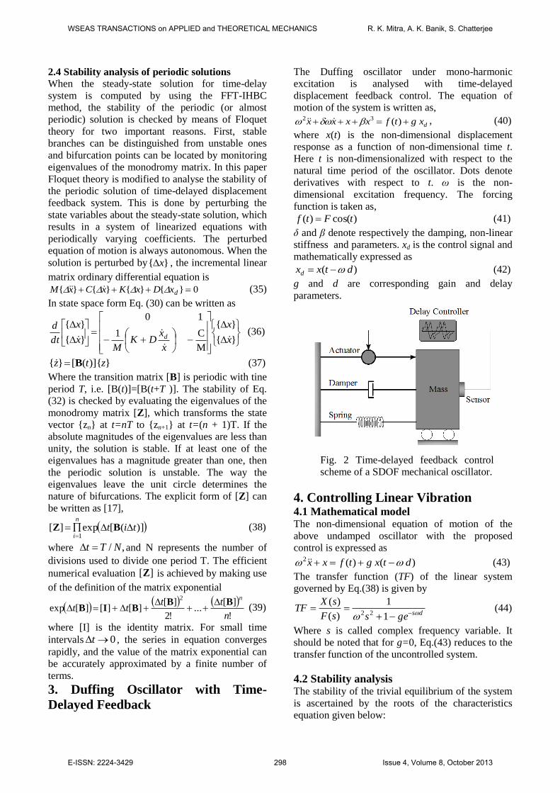
3. Duffing Oscillator with Time-

Delayed Feedback

The Duffing oscillator under mono-harmonic

excitation is analysed with time-delayed

displacement feedback control. The equation of

motion of the system is written as,

dxgtfxxxx )(32 , (40)

where x(t) is the non-dimensional displacement

response as a function of non-dimensional time t.

Here t is non-dimensionalized with respect to the

natural time period of the oscillator. Dots denote

derivatives with respect to t. ω is the non-

dimensional excitation frequency. The forcing

function is taken as,

)cos()( tFtf (41)

δ and β denote respectively the damping, non-linear

stiffness and parameters. xd is the control signal and

mathematically expressed as

) ( dtxxd (42)

g and d are corresponding gain and delay

parameters.

Fig. 2 Time-delayed feedback control

scheme of a SDOF mechanical oscillator.

4. Controlling Linear Vibration 4.1 Mathematical model The non-dimensional equation of motion of the

above undamped oscillator with the proposed

control is expressed as

) ( )(2 dtxgtfxx (43)

The transfer function (TF) of the linear system

governed by Eq.(38) is given by

dsgessF

sXTF

1

1

)(

)(22

(44)

Where s is called complex frequency variable. It

should be noted that for g=0, Eq.(43) reduces to the

transfer function of the uncontrolled system.

4.2 Stability analysis The stability of the trivial equilibrium of the system

is ascertained by the roots of the characteristics

equation given below:



0122 dsges (45)

Substituting js ( 1j and is any real

number) in Eq.(45) and separating the imaginary

and real parts yields,

0)cos(1 22 dg (46a)

and 0)sin( dg (46b)

Since g can't be zero,

0)sin( d (47)

The general solution of Eq.(46b) is

, nd ,...,2,1,0n (48)

Substituting Eq.(48) into (46a), yields the following

equation for the critical stability lines:

0)cos(1

2

ng

d

n (49)

As the uncontrolled system is marginally stable,

0g is also a critical stability line. Finally, the

stable regions in the g vs. d plane are obtained from

the sign of the root tendency defined below [12],

),(d

dResgn),(

cc dj

ccd

sdR

(50)

R

Increase in the

number of unstable

roots

Decrease in the

number of unstable

roots

+1 2

-1 2

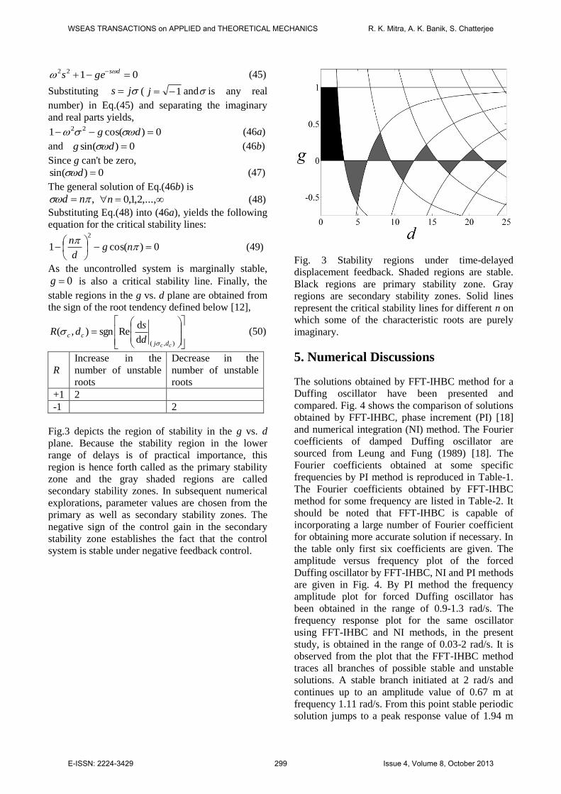
Fig.3 depicts the region of stability in the g vs. d

plane. Because the stability region in the lower

range of delays is of practical importance, this

region is hence forth called as the primary stability

zone and the gray shaded regions are called

secondary stability zones. In subsequent numerical

explorations, parameter values are chosen from the

primary as well as secondary stability zones. The

negative sign of the control gain in the secondary

stability zone establishes the fact that the control

system is stable under negative feedback control.

Fig. 3 Stability regions under time-delayed

displacement feedback. Shaded regions are stable.

Black regions are primary stability zone. Gray

regions are secondary stability zones. Solid lines

represent the critical stability lines for different n on

which some of the characteristic roots are purely

imaginary.

5. Numerical Discussions

The solutions obtained by FFT-IHBC method for a

Duffing oscillator have been presented and

compared. Fig. 4 shows the comparison of solutions

obtained by FFT-IHBC, phase increment (PI) [18]

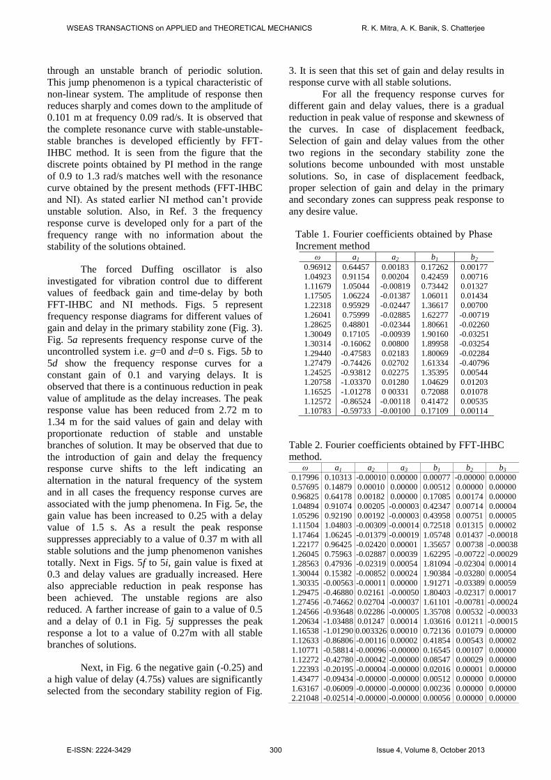
and numerical integration (NI) method. The Fourier

coefficients of damped Duffing oscillator are

sourced from Leung and Fung (1989) [18]. The

Fourier coefficients obtained at some specific

frequencies by PI method is reproduced in Table-1.

The Fourier coefficients obtained by FFT-IHBC

method for some frequency are listed in Table-2. It

should be noted that FFT-IHBC is capable of

incorporating a large number of Fourier coefficient

for obtaining more accurate solution if necessary. In

the table only first six coefficients are given. The

amplitude versus frequency plot of the forced

Duffing oscillator by FFT-IHBC, NI and PI methods

are given in Fig. 4. By PI method the frequency

amplitude plot for forced Duffing oscillator has

been obtained in the range of 0.9-1.3 rad/s. The

frequency response plot for the same oscillator

using FFT-IHBC and NI methods, in the present

study, is obtained in the range of 0.03-2 rad/s. It is

observed from the plot that the FFT-IHBC method

traces all branches of possible stable and unstable

solutions. A stable branch initiated at 2 rad/s and

continues up to an amplitude value of 0.67 m at

frequency 1.11 rad/s. From this point stable periodic

solution jumps to a peak response value of 1.94 m



through an unstable branch of periodic solution.

This jump phenomenon is a typical characteristic of

non-linear system. The amplitude of response then

reduces sharply and comes down to the amplitude of

0.101 m at frequency 0.09 rad/s. It is observed that

the complete resonance curve with stable-unstable-

stable branches is developed efficiently by FFT-

IHBC method. It is seen from the figure that the

discrete points obtained by PI method in the range

of 0.9 to 1.3 rad/s matches well with the resonance

curve obtained by the present methods (FFT-IHBC

and NI). As stated earlier NI method can’t provide

unstable solution. Also, in Ref. 3 the frequency

response curve is developed only for a part of the

frequency range with no information about the

stability of the solutions obtained.

The forced Duffing oscillator is also

investigated for vibration control due to different

values of feedback gain and time-delay by both

FFT-IHBC and NI methods. Figs. 5 represent

frequency response diagrams for different values of

gain and delay in the primary stability zone (Fig. 3).

Fig. 5a represents frequency response curve of the

uncontrolled system i.e. g=0 and d=0 s. Figs. 5b to

5d show the frequency response curves for a

constant gain of 0.1 and varying delays. It is

observed that there is a continuous reduction in peak

value of amplitude as the delay increases. The peak

response value has been reduced from 2.72 m to

1.34 m for the said values of gain and delay with

proportionate reduction of stable and unstable

branches of solution. It may be observed that due to

the introduction of gain and delay the frequency

response curve shifts to the left indicating an

alternation in the natural frequency of the system

and in all cases the frequency response curves are

associated with the jump phenomena. In Fig. 5e, the

gain value has been increased to 0.25 with a delay

value of 1.5 s. As a result the peak response

suppresses appreciably to a value of 0.37 m with all

stable solutions and the jump phenomenon vanishes

totally. Next in Figs. 5f to 5i, gain value is fixed at

0.3 and delay values are gradually increased. Here

also appreciable reduction in peak response has

been achieved. The unstable regions are also

reduced. A farther increase of gain to a value of 0.5

and a delay of 0.1 in Fig. 5j suppresses the peak

response a lot to a value of 0.27m with all stable

branches of solutions.

Next, in Fig. 6 the negative gain (-0.25) and

a high value of delay (4.75s) values are significantly

selected from the secondary stability region of Fig.

3. It is seen that this set of gain and delay results in

response curve with all stable solutions.

For all the frequency response curves for

different gain and delay values, there is a gradual

reduction in peak value of response and skewness of

the curves. In case of displacement feedback,

Selection of gain and delay values from the other

two regions in the secondary stability zone the

solutions become unbounded with most unstable

solutions. So, in case of displacement feedback,

proper selection of gain and delay in the primary

and secondary zones can suppress peak response to

any desire value.

Table 1. Fourier coefficients obtained by Phase

Increment method ω a1 a2 b1 b2

0.96912

1.04923

1.11679

1.17505

1.22318

1.26041

1.28625

1.30049

1.30314

1.29440

1.27479

1.24525

1.20758

1.16525

1.12572

1.10783

0.64457

0.91154

1.05044

1.06224

0.95929

0.75999

0.48801

0.17105

-0.16062

-0.47583

-0.74426

-0.93812

-1.03370

-1.01278

-0.86524

-0.59733

0.00183

0.00204

-0.00819

-0.01387

-0.02447

-0.02885

-0.02344

-0.00939

0.00800

0.02183

0.02702

0.02275

0.01280

0 00331

-0.00118

-0.00100

0.17262

0.42459

0.73442

1.06011

1.36617

1.62277

1.80661

1.90160

1.89958

1.80069

1.61334

1.35395

1.04629

0.72088

0.41472

0.17109

0.00177

0.00716

0.01327

0.01434

0.00700

-0.00719

-0.02260

-0.03251

-0.03254

-0.02284

-0.40796

0.00544

0.01203

0.01078

0.00535

0.00114

Table 2. Fourier coefficients obtained by FFT-IHBC

method. ω a1 a2 a3 b1 b2 b3

0.17996 0.10313 -0.00010 0.00000 0.00077 -0.00000 0.00000

0.57695 0.14879 0.00010 0.00000 0.00512 0.00000 0.00000

0.96825 0.64178 0.00182 0.00000 0.17085 0.00174 0.00000

1.04894 0.91074 0.00205 -0.00003 0.42347 0.00714 0.00004

1.05296 0.92190 0.00192 -0.00003 0.43958 0.00751 0.00005

1.11504 1.04803 -0.00309 -0.00014 0.72518 0.01315 0.00002

1.17464 1.06245 -0.01379 -0.00019 1.05748 0.01437 -0.00018

1.22177 0.96425 -0.02420 0.00001 1.35657 0.00738 -0.00038

1.26045 0.75963 -0.02887 0.00039 1.62295 -0.00722 -0.00029

1.28563 0.47936 -0.02319 0.00054 1.81094 -0.02304 0.00014

1.30044 0.15382 -0.00852 0.00024 1.90384 -0.03280 0.00054

1.30335 -0.00563 -0.00011 0.00000 1.91271 -0.03389 0.00059

1.29475 -0.46880 0.02161 -0.00050 1.80403 -0.02317 0.00017

1.27456 -0.74662 0.02704 -0.00037 1.61101 -0.00781 -0.00024

1.24566 -0.93648 0.02286 -0.00005 1.35708 0.00532 -0.00033

1.20634 -1.03488 0.01247 0.00014 1.03616 0.01211 -0.00015

1.16538 -1.01290 0.003326 0.00010 0.72136 0.01079 0.00000

1.12633 -0.86806 -0.00116 0.00002 0.41854 0.00543 0.00002

1.10771 -0.58814 -0.00096 -0.00000 0.16545 0.00107 0.00000

1.12272 -0.42780 -0.00042 -0.00000 0.08547 0.00029 0.00000

1.22393 -0.20195 -0.00004 -0.00000 0.02016 0.00001 0.00000

1.43477 -0.09434 -0.00000 -0.00000 0.00512 0.00000 0.00000

1.63167 -0.06009 -0.00000 -0.00000 0.00236 0.00000 0.00000

2.21048 -0.02514 -0.00000 -0.00000 0.00056 0.00000 0.00000



Fig. 4. Frequency response curves of uncontrolled

system (δ=0.04, β=0.25, F=0.1, g=0, d=0).



Fig. 5. Frequency response diagram for different

gain (positive) and delay in the secondary stability

zone ( δ=0.02, β=0.25, F=0.1

Fig. 6. Frequency response diagrams for gain

(negative) and delay in the secondary stability zone

(δ=0.02, β =0.25, F=0.1)

6. Conclusions

The Duffing oscillator under monoharmonic

excitation is investigated for desired

suppression of peak response by intentional

time-delayed displacement feedback. The

following conclusions are drawn:

The computation of Jacobian matrix and

hence periodic solution is highly efficient

and faster in comparison to simple IHB

method.

A large number of harmonics can be

incorporated in FFT-IHBC, if necessary;

whereas simple IHB method encounters

difficulty with large number of harmonics.

The solutions obtained by NI matches

perfectly with stable solutions obtained by

FFT-IHBC method.

FFT-IHBC can conveniently handle any

type of nonlinearity whereas nonlinearity

after necessary transformation amenable to

IHB method can only be handled by simple

IHB method.

The complete frequency response curve

with all possible stable and unstable

solution and solution branches can be very

efficiently developed by FFT-IHBC method

and jump etc. can be observed.

The introduction of gain delay in the forced

Duffing oscillator results in appreciable

reduction in the peak value of response.



For g=0.3 and d=0.4 s all solutions become

stable and jump phenomena is no longer

observed.

It is observed that appropriate selection of

gain and delay parameters in intentional

time-delayed feedback significantly changes

the resonances curves and stability of

solutions and sometimes in better

suppression of vibrations.

References:

[1] K. Gu, and S. Niculescu, Survey on Recent

Results in the Stability and Control of Time-

delay Systems, ASME Journal of Dynamic

Systems, Measurements and Control, 125 (2003)

158-165.

[2] N. Olgac, B.T. Holm-Hansen, A novel active

vibration absorption technique: delayed

resonator, Journal of Sound and Vibration 176

(1994) 93–104.

[3] N. Jalili, N. Olgac, Multiple identical delayed-

resonator vibration absorbers for multi-degree-of

freedom mechanical structures, Journal of

Dynamic Systems, Measurement, and Control,

ASME 122 (2000) 314–322.4.

[4] H. Hu, E.H. Dowell, L.N. Virgin, Resonances of

a harmonically forced Duffing oscillator with

time-delay state feedback, Nonlinear Dynamics

15 (1998) 311–327.

[5] F.E. Udwadia, H. von Bremen, R. Kumar, M.

Hosseini, Time-delayed control of structures,

Earthquake Engineering and Structural

Dynamics 32 (2003) 495–535.

[6] F.E. Udwadia, H. von Bremen, P. Phohomsiri,

Time-delayed control design for active control of

structures: principles and application, Structural

Control Health Monitoring 12 (3) (2005).

[7] P. Phohomsiri, F.E. Udwadia, H.F. von Bremen,

Time-delayed positive velocity feedback control

design for active control of structures, Journal of

Engineering Mechanics, ASCE (2006) 690–703.

[8] A. Maccari, Vibration control for parametrically

excited Lie´nard systems, International Journal

of Non-Linear Mechanics 41 (2006) 146–155.

[9] F.M. Atay, Van der Pol’s oscillator under

delayed feedback, Journal of Sound and

Vibration 218 (1998) 333–339.

[10] A. Maccari, Vibration control for the primary

resonance of a cantilever beam by a time-delay

state feedback, Journal of Sound and Vibration

259 (2003) 241–251.

[11] S. Chatterjee, Time-delayed feedback control

of friction induced instabilities, International

Journal of Non-Linear Mechanics 42 (9) (2007)

1127–1143.

[12] S. Chatterjee, “Vibration control by recursive

time-delayed acceleration feedback”, Journal of

Sound and Vibration, 317 (2008) 67–90.

[13] Y. M. Ram, A. Singh, and J. E. Mottershead,

State feedback control with time-delay”,

Mechanical Systems and Signal Processing, 23

(2009) 1940–1945.

[14] A. F. El-Bassiouny, and S. El-kholy,

Resonances of a non-linear SDOF system with

time-delay in linear feedback control”, Physica

Scripta, 81 (2009) no.1.

[15] A. Y. T. Leung, and S. K. Chui, Non-linear

vibration of coupled Duffing oscillator by an

improved incremental harmonic balance method,

Journal of sound and vibration 181(4), (1995)

619-633.

[16] A. K. Banik, and T. K. Datta, Stability Analysis

of Two-Point Mooring System in Surge

Oscillation, ASME, Journal of Computational

and Nonlinear Dynamics, Vol. 5, 021005-1

(2010).

[17] P. Friedmann, C. E Hammond, and T. H. Woo,

Efficient Numerical Treatment of Periodic

Systems With Application to Stability Problems,

International Journal of Numerical. Methods in

Engineering, 11 (1997) 1117–1136.

[18] A. Y. T. Leung, and T. C. Fung, Phase

increment analysis of damped Duffing

oscillators, Internal Journal of numerical

methods in engineering, Vol. 28 (1989).193-209.



dynamic stability of time-delayed feedback control system ... · dynamic stability of time-delayed...

Documents