Dynamic Risk Management: Theory and Evidence∗

Frank Fehle and Sergey Tsyplakov

September 2, 2003

∗Frank Fehle is at Barclays Global Investors and the University of South Carolina; E-Mail: ffehle@moore.sc.edu;

Phone: (803) 777-6980. Sergey Tsyplakov is at the University of South Carolina; E-Mail: sergey@moore.sc.edu;

Phone: (803) 777-4669. Fax: (803) 777-6876. Mailing address: BFIRE, Moore School of Business, University of South

Carolina, Columbia, SC 29208. We would like to thank seminar participants at 2003 Annual Meeting of the Western

Finance Association, the University of South Carolina, and, especially, Tim Adam, Shingo Goto, David Haushalter,

Ted Moore, Greg Niehaus, Ajay Patel, Sheridan Titman, Stathis Tompaidis, and Donghang Zhang. Authors are

grateful to the Caesarea Center and the Western Finance Association for awarding this paper for the 2003 best paper

on risk management. The views and opinions expressed in this paper are the authors’ and do not represent Barclays

Global Investors.

Dynamic Risk Management: Theory and Evidence

Abstract

We present and tests an infinite horizon, continuous time model of a firm that can dynamically adjust

the use and maturity of risk management instruments whose purpose is to reduce product price uncertainty

thereby mitigating financial distress losses. The dynamic setting relaxes several restricting assumptions

common to static models. Specifically, we assume that 1) the firm can adjust its use of risk management

instruments over time, 2) risk management instruments expire as time progresses and that the available

maturity of the risk management instruments is shorter than the life time of the firm, and 3) there are

transaction costs associated with initiation and adjustment of risk management contracts. The model pro-

duces a number of new time series and cross-sectional implications on how firms use short-term instruments

to hedge long-term cash flow uncertainty. Numerical results describe the optimal timing, adjustment, and

rolling-over of risk management instruments, and the choice of contract maturity in response to changes in

the firm’s product price. The model predicts that firms that are either far from financial distress or deep

in financial distress neither initiate nor adjust their risk management instruments, while firms between the

two extremes initiate and actively adjust and/or roll-over their risk management instruments. Using quar-

terly panel data on gold mining firms between 1993 and 1999, the paper finds evidence of a non-monotonic

relation between measures of financial distress and risk management activity consistent with the model.

We also provide evidence supportive of the model’s predictions with respect to the maturity choice of risk

management contracts.

JEL Classifications: G30, G32, G33.

Keywords: risk management, dynamic, maturity choice, distress, default, transaction costs.

1 Introduction

Much of our understanding of corporate risk management is based on static models that describe how

various capital market imperfections give firms an incentive to reduce risk. While existing models

provide rich intuition as to why firms should manage risk, they provide fewer predictions about how

firms translate the incentives to manage risk into actual decisions on the choice of risk management

instruments and how these strategies evolve over time.

Our main contribution is to present and test a dynamic model of corporate risk management in

a continuous-time and infinite-horizon framework.1 We analyze issues, which are difficult to address

in static models, including the optimal timing to initiate risk management contracts, early termi-

nation, replacement of expiring and terminated contracts, contract maturity choice, and frequency

of adjustment. Many static models assume that firms make one-period decisions to hedge and that

these decisions are irreversible and costless.2 Therefore one-period models also often implicitly as-

sume that the employed risk management instruments have the same duration as the lifetime of

the firm. Treating risk management choices as irreversible limits the ability of the static models to

recognize the value of dynamic risk management in adapting to changes in market conditions and

firm characteristics. The fact that most risk management instruments have shorter maturities than

the duration of the firm’s operations has important implications for the timing and sequence of risk

management decisions and it provides an intuition for the limited effect of risk management on firm

exposures observed in empirical studies such as Geczy, Minton, and Schrand (1999), Petersen and

Thiagarajan (2000), and Allayannis, Brown, and Klapper (2001).

Following the static model of Smith and Stulz (1985), our model motivates risk management via

financial distress costs which are incurred when the firm’s product price declines below costs.3 As

a consequence, the model captures the suggestion by Stulz (1996) that firms use risk management

not to reduce volatility per se but rather to avoid costly lower-tail outcomes that lead to financial

distress. In our model the firm chooses both the timing and maturity of hedging contracts where the

1Other papers on hedging that use a continuous-time framework include Stulz (1984), Ho (1984) and Leland (1998).2Throughout the remainder of the paper the terms hedging and risk management are used interchangeably3Although not explicitly modelled, the framework can also accommodate costly external financing as in Froot,

Scharfstein, and Stein (1993) as an incentive to manage risk. The model does not directly incorporate other incentives

to manage risk which are suggested by existing static theories such as for example taxes (Smith and Stulz (1985)),

information asymmetry between managers and investors (DeMarzo and Duffie (1991)), or managerial risk aversion

(Smith and Stulz (1985)). Stulz (2002) provides an up-to-date review of risk management rationales.

1

maximum available maturity is shorter than the duration of the firm’s operations and expected cash

flows. Hedging contracts are modelled as a portfolio of forward contracts (with an initial contract

value of zero) on the firm’s product price which is the source of uncertainty in the model evolving as

a stochastic process.

In the model the firm faces the question of how to use short-term instruments to hedge long-term

operations. Moreover, in a multiperiod dynamic setting, the firm constantly faces the problem that

hedging positions entered into earlier may loose their effectiveness as product prices change during

the maturity of the contract. Thus, the firm continuously reevaluates and decides whether and how

often to adjust its hedging position before expiration, or to wait and keep an existing contract and to

enter a new position (if any) upon expiration. We also model the transaction costs associated with

both the initiation and early termination of risk management contracts, which complicates the firm’s

problem further. On one hand, longer term contracts are more favorable since the firm does not have

to replace its contracts very frequently. On the other hand, longer-term contracts are less flexible and

incur transaction costs should the firm decide to terminate them before they expire. The idea that

transaction costs are important determinants of risk management decisions is supported by empirical

research such as Nance, Smith and Smithson (1993), Mian (1996), and Geczy, Minton and Schrand

(1997) who find evidence consistent with economies of scale of risk management. In practice, the

finite life of risk management instruments is most obvious where derivative securities are concerned:

there are few liquid derivative security markets (OTC or exchange) which offer maturities beyond ten

years. Thus, the theoretical results are most applicable to risk management via derivative securities

or other financial risk management contracts. However, arguably even other risk management tools,

such as operational hedges, may have a maturity which is shorter than the firm’s potentially infinite

horizon, and therefore eventually may have to be replaced as their effects expire.

A number of new insights arise from the model with respect to both the time-series and cross-

sectional properties of risk management strategies. First, the model implies that there is a non-

monotonic relation between risk management activity and product price (and firm leverage). For a

firm with fixed debt, the optimal risk management strategy depends on the spot level of the firm’s

product price, relative to the firm’s total costs. At very high prices, firms neither initiate new risk

management contracts nor adjust existing contracts as financial distress is not imminent. As prices

fall and financial distress becomes more likely, firms enter the active risk management zone in which

they are more likely to initiate risk management contracts and actively replace and roll them over in

order to avoid financial distress. However, as prices fall further, and firms become deeply distressed,

2

they are again less likely to initiate or adjust risk management contracts. Cross-sectionally, the

model suggests a similar non-monotonic relation between factors such as leverage, which affect the

likelihood of financial distress, and risk management. While this non-monotonic relation has been

suggested previously by Stulz (1996), our model is the first to explicitly generate the relation from a

dynamic model.4

Secondly, the paper provides new results regarding the maturity choice of risk management con-

tracts. Our model indicates that more deeply distressed firms tend to choose shorter maturities for

newly initiated risk management instruments. Also, the model predicts that firms with higher trans-

action costs tend to change their risk management contracts less often and choose longer maturities.

The results also imply that a firm with greater product price volatility chooses risk management

contracts with longer maturity.

With respect to the optimal adjustment of risk management instruments, the optimal roll-over

strategy of risk management contracts is quite different from mechanical replacement of expiring

contracts. Optimal roll-over and replacement decisions depend on the features of risk management

contracts already in place, which are more likely to be replaced before they mature if they are out-of-

the-money. For portfolio of forwards contracts, this implies that the frequency of risk management

contract adjustments should be higher during periods of rising spot prices than during periods of

falling spot prices. The features of existing contracts, such as moneyness and remaining maturity, are

determined by the historic path of the spot price. Empirically, this implies that firms with identical

characteristics which are observed at different points in time but with the same market conditions

may have very different risk management contracts in place because the observed firms may have

reached a given state via different paths. Similarly, identical firms at the same current spot price

may have differing risk management contracts in place, if their histories of firm-level characteristics

(e.g. leverage) are different. Therefore, in some cases empirical tests of risk management rationales

could be improved by incorporating information about the preceding price and firm history.

To illustrate the applicability of the model, its parameters are calibrated to be consistent with

empirical observations of firms in the gold mining industry. Specifically, parameter values are selected

that roughly match the time-series properties of gold price returns and the financial ratios and

production costs of gold mining firms during the sample period of 1993 to 1999, which is used for the

4The non-monotonic relation is also consistent with evidence such as Mian (1996), Tufano (1996), and Geczy,

Minton, and Schrand (1997) finding only weak evidence that proxies of distress costs have a positive monotonic effect

on corporate risk management.

3

empirical work. Given the calibrated parameters, we show that optimal risk management policies

may have little impact on equity volatility, which is consistent with existing empirical findings. The

reason is that, at a given time, only the portion of the firm’s future cash flows, which occur during

the risk management instruments’ finite duration, can be hedged.

Several predictions of the model are tested using quarterly derivatives use data for gold mining

firms between 1993 and 1999. We employ a similar measure of risk management activity as in Tufano

(1996), and Brown, Crabb, and Haushalter (2001). The empirical tests regarding risk management

activities do not provide a comprehensive analysis of all existing models, but rather focus on some

of the new predictions motivated by our model. The empirical tests indicate that there is indeed

evidence of non-monotonicity between the measure of risk management activity and the likelihood

of distress as proxied by several measures such as leverage and quick ratio. We also find a significant

relation between gold spot prices and risk management activity as suggested by the model.

The tests also extend the existing empirical literature by contributing an analysis of maturity

choice of risk management instruments. Based on a measure of the weighted-average maturity of

a firm’s risk management contracts, we find evidence of a non-monotonic relation between leverage

and maturity consistent with the model’s predictions.

The remainder of the paper proceeds as follows: the next section introduces the model, and then

solutions for the valuation of the firm’s equity and the choice of the risk management strategy are

provided in section 3; section 4 provides numerical results. Empirical evidence is presented in section

5. Section 6 concludes.

2 Dynamic Risk Management Theory

2.1 Overview

This section develops a continuous time, infinite horizon model of a firm which endogenously and

dynamically adjusts its risk management contract which is a function of the firm’s exogenous product

price.

The model can be described by the following timeline:

At time 0

◦ The levered firm decides whether to initiate a risk management contract (guaranteeing a set of

forward prices for a certain fraction of the firm’s output), and chooses its maturity.

4

Each subsequent time period

◦ The firm produces one unit of product at a fixed cost and realizes cash flows that are determinedby the current spot price and the price guaranteed by the risk management contract (if any)

and whether or not the firm is in financial distress.

◦ The firm can default, in which case the debtholders recover part of the firm’s value and the

equityholders get nothing and are obligated to terminate (pay out or cash out) any outstanding

risk management contracts, or,

◦ If not in default, the firm meets its periodic debt payments and pays production costs, and then

makes a decision with respect to its risk management strategy, i.e.

• the firm can enter a risk management contract and choose its maturity;

• if the firm currently operates with a risk management contract in place, it can choose to

terminate the contract early and to cash out (or to pay out) its current position at a fair

market value. Both the initiation and the termination of the risk management contract generate

transaction costs.

◦ The residual cash flow after debt payments and production costs is paid to the equityholders asdividends.

The firm is assumed to default on its debt optimally, i.e. when the market value of the firm’s

equity becomes zero. The firm’s decisions with respect to the risk management strategy are made

from the perspective of the shareholders who maximize the value of their equity stake.5 Both equity

and debt are priced fairly taking into account the risk management strategy of the equityholders.

Because of a need to limit the dimensionality of the model, we are forced to make several modeling

compromises. First, we do not allow the firm to change the structure of its debt over time. Second,

we assume that the firm holds no cash, which implies that it pays all its residual cash flows as

dividends. The following subsections present a detailed description of the model.

5For comparison reasons we can also consider the choice of the risk management policy from the perspective of all

claimholders of the firm to maximize the total value of the firm’s debt and equity.

5

2.2 Spot Price and Production Costs

The firm continuously produces a unit of product, which can for example be viewed as a commodity,

whose spot price p, continuously evolves through time and is described by the log-normal process:6

dp

p= (r − a)dt+ σdWp (1)

where Wp is a Weiner process under the risk neutral measure Q, σ is the instantaneous volatility

coefficient, r is the risk free rate which is assumed to be constant and a, (a ≥ 0), is the convenienceyield. The cost of production of one unit of product c (c ≥ 0) is assumed to be constant. Revenueuncertainty driven by variation in the output spot price is the only source of uncertainty explicitly

modelled. In this sense the results will be most applicable to firms facing less cost uncertainty and

more revenue uncertainty such as firms in many extraction industries (oil, gold, etc.) which have

fairly predictable production costs.

2.3 Risk Management Contracts

At any time the firm can choose to enter (or terminate, if any) a risk management contract that aims

to reduce temporarily the risk related to the product’s price uncertainty.7 The risk management

contract guarantees a predetermined price for a fixed fraction h, (0 ≤ h ≤ 100%), of the firm’s

product for the chosen maturity τ . When the firm enters a new risk management contract, it chooses

the contract’s maturity τ , τ ≤ T, where T is the maximum maturity available.

Parameter h is constant and can be viewed as the hedge ratio, which determines what portion of

the cash flow is hedged. While the hedge ratio can potentially be endogenized in the model, we believe

that this would add further complexity and distract from the focus of the current analysis which is the

optimal timing and maturity choice of risk management contracts.8 However, we provide comparative

statics in section 4.3.2 to assess the effect of different levels of the hedge ratio parameter. While spot

price uncertainty for the firm’s product is the only source of uncertainty explicitly modelled, choosing

6The model can easily be extended for any reasonable price process. For example, we can assume that the price

follows a mean reverting process of the Ornstein-Uhlenbeck type, or the two factor process introduced in Gibson and

Schwartz (1990).7We assume that the production quantity is non-stochastic. Static models that incorporate quantity risk include

Koppenhaver (1985), Morgan, Shome, and Smith (1988), and Brown and Toft (2002).8Static models that incorporate the choice of the hedge ratio include Froot, Sharfstein and Stein (1993), and

Kerkvliet and Moffett (1991).

6

a fixed hedge ratio of less than 100% is also a simple way to assess the effect of additional (non-

hedgeable) “background” risk which is not explicitly modelled in the current setting.

The risk management contract consists of a portfolio (continuum) of infinitesimally small (in

terms of notional amount) fairly priced forward contracts with continuous maturities between 0 and

τ .9 At the moment of origination, the risk management contract has zero expected value. Given

the level of the spot price pt at origination, the risk management contract guarantees the price of

p∗t = pt at the current time t, and in the next period t + ∆t the contract guarantees the price of

p∗t+∆t = pt ·e(r−a)∆t, two periods from t the contract guarantees the price of p∗t+2∆t = pt ·e(r−a)2∆t, andso on until maturity. The entire contract guarantees the firm a price schedule for its product {p∗t ,p∗t+∆t, p

∗t+2∆t, ...., p

∗t+τ} = {pt, pt · e(r−a)∆t, pt · e(r−a)2∆t, ...., pt · e(r−a)τ} during the contract maturity

τ , (τ ≤ T ). Thus, each risk management contract can be uniquely described by a pair {p∗, τ}, wherep∗ is the contract guaranteed price at which the firm is entitled to sell its product at the current

time t, and τ is the time remaining in the contract before it matures. At a given time, p∗ is sufficient

to uniquely calculate the prices of the remaining maturity predetermined by contract. Although,

initially the contract has expected value of zero, its value (“moneyness”) will fluctuate as the spot

price changes and maturity gradually declines.

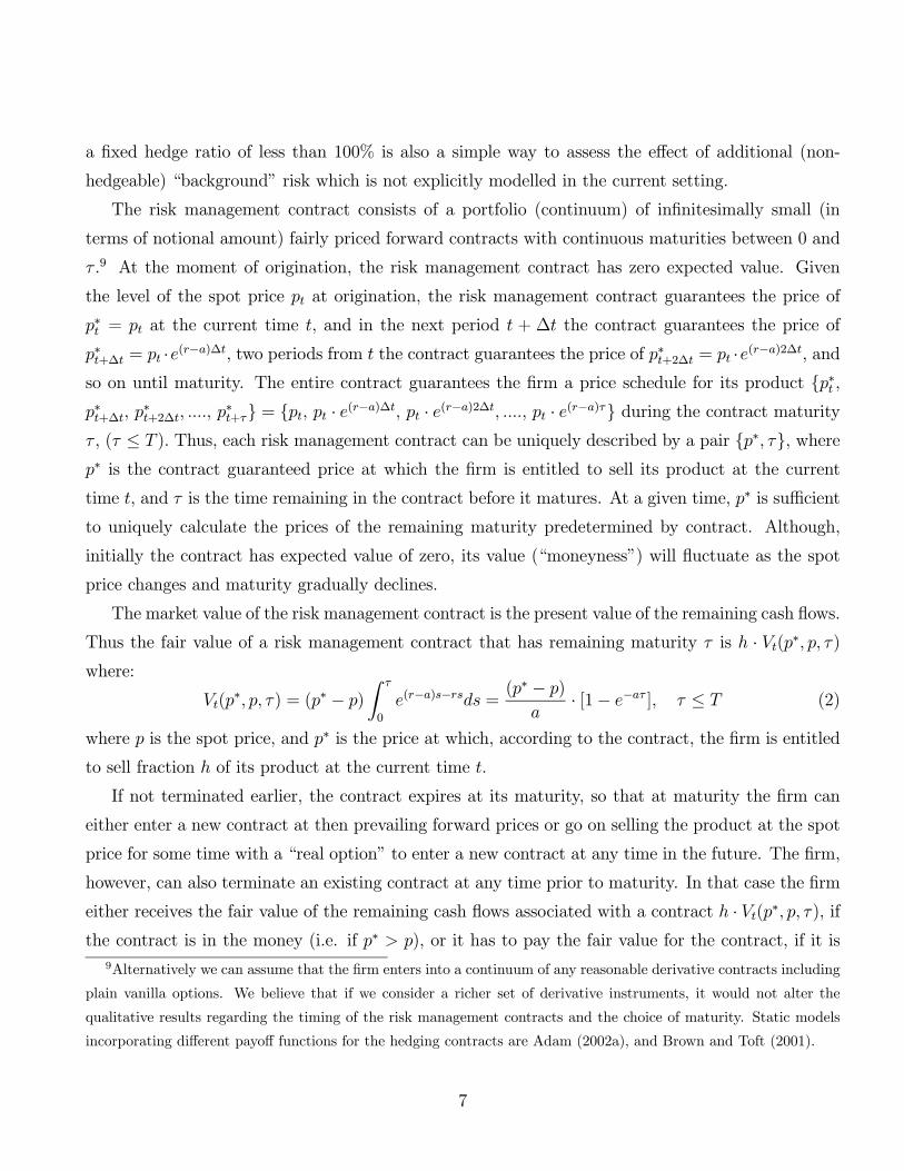
The market value of the risk management contract is the present value of the remaining cash flows.

Thus the fair value of a risk management contract that has remaining maturity τ is h · Vt(p∗, p, τ)where:

Vt(p∗, p, τ) = (p∗ − p)

Z τ

0

e(r−a)s−rsds =(p∗ − p)a

· [1− e−aτ ], τ ≤ T (2)

where p is the spot price, and p∗ is the price at which, according to the contract, the firm is entitled

to sell fraction h of its product at the current time t.

If not terminated earlier, the contract expires at its maturity, so that at maturity the firm can

either enter a new contract at then prevailing forward prices or go on selling the product at the spot

price for some time with a “real option” to enter a new contract at any time in the future. The firm,

however, can also terminate an existing contract at any time prior to maturity. In that case the firm

either receives the fair value of the remaining cash flows associated with a contract h · Vt(p∗, p, τ), ifthe contract is in the money (i.e. if p∗ > p), or it has to pay the fair value for the contract, if it is

9Alternatively we can assume that the firm enters into a continuum of any reasonable derivative contracts including

plain vanilla options. We believe that if we consider a richer set of derivative instruments, it would not alter the

qualitative results regarding the timing of the risk management contracts and the choice of maturity. Static models

incorporating different payoff functions for the hedging contracts are Adam (2002a), and Brown and Toft (2001).

7

out of the money (i.e. if p∗ < p).

We assume that the firm has to pay constant transaction costs TC when it initiates a new con-

tract and terminates a contract initiated earlier.10 Such fixed transaction costs can occur both due

to fixed components of trading costs such as brokerage fees as well as due to fixed cost components

of administering the risk management contract within the firm (e.g. internal reporting and account-

ing). The firm adjusts its risk management contracts in a discrete manner since the transaction

costs preclude the firm from performing continuous adjustment and roll-over of its risk management

position.

One possible risk management strategy for the firm is to adjust and roll-over its risk management

contracts in the sense that the firm can always replace an existing risk management contract with a

new contract of longer maturity by simultaneously terminating the current risk management contract

and initiating a new one at the prevailing spot price. Hereby the firm faces a trade-off between

incurring transaction costs and operating with a potentially suboptimal contract entered into earlier.

It would be more realistic to allow the firm to have multiple hedging contracts with overlapping

maturities. However, that would result in a more complicated hedging structure. Therefore, in order

to avoid the need for tracking the multiple contracts and their maturities, we assume that the firm

adjusts its hedging position by repurchasing its current hedging contract and entering a new one.

2.4 Debt and Firm Cash Flow

We assume that the firm issues a perpetual non-callable coupon bond. The amount of debt is

exogenous and stationary and the equityholders pay a continuous coupon d. The firm uses its income

to meet its debt obligation, with any residual being paid out as a dividend to the equityholders. In

practice, a firm may retain part of its cash flow and then use it for future debt service, which may

affect the risk management strategy and the valuation of equity. Similarly, we ignore the option

to store the product and to time the sale of the product. Although feasible, incorporating these

features would lead to an increase in the dimensionality of the model and would further complicate

the analysis.

The firm’s income depends on whether or not the firm has a risk management contract. Thus, the

firm’s instantaneous dividend at any time t equals either p−c−d if the firm has no risk management10Transaction costs of initiating the portfolio of futures contracts can also be associated with the requirement to

post margin at the clearinghouse. Bid-ask spreads and execution costs may also be viewed as a part of the overall

transaction costs of a risk management program. (see Ferguson and Mann (2001))

8

contract outstanding, or h ·p∗+(1−h)p− c−d otherwise, where p∗ is the price according to the riskmanagement contract originated earlier, c is the constant cost of production of one unit of product.

If there is insufficient cash flow to meet the debt payment, the firm can raise capital by issuing

equity. The conditions under which outside capital can be raised, and the costs associated with

raising it, will be described in the next section.

By assuming that the firm operates with static debt we ignore potential interactions between

capital structure and risk management decisions. In principle, it is possible to extend the model

by allowing equityholders to change the level of the debt dynamically as it was done in Mauer and

Triantis (1993) or in Titman and Tsyplakov (2002).

2.5 Financial Distress

When the firm’s instantaneous cash flow cannot cover the debt payments, the firm experiences

financial distress. In this situation the firm is required to issue equity. We assume that in financial

distress the firm incurs additional cash flow losses because customers, suppliers, or strategic partners

may not be willing to deal with financially distressed companies. Unlike default costs that are

incurred by debtholders at bankruptcy, distress costs are directly borne by equityholders. These

costs are important because they may be incurred long before bankruptcy is imminent and they

provide incentives to manage risk. While the requirement of insufficient cash flows is convenient for

modelling purposes, in practice, financial distress can occur even when cash flows are low relative to

required debt payments but are not yet insufficient.

The magnitude of financial distress costs in the model is determined by how low the firm’s cash

flow falls relative to the debt payments and production costs. We assume that financial distress costs

are proportional to the difference between the firm’s required debt payments and its income net of

production costs. Specifically, if the firm’s dividend rate is negative, i.e.

p0 − c− d < 0, (3)

then the firm incurs distress costs equal to

CPDistressmax[0, − p0 + c+ d], (4)

where CPDistress is constant, and p0 equals either the spot price pt (if the firm does not have an outstand-

ing risk management contract) or otherwise, p0 = hp∗+(1−h)p, where p∗ is the price predetermined

9

by the risk management contract. The firm with a risk management contract outstanding may also

be in distress if the price guaranteed by the contract is below the debt payments, while the spot price

can actually be above it.

Financial distress, as modeled here, does not create any permanent damage to the firm, but rather

causes temporary cash flow loss. In other words, the distress situation does not directly affect the

future productivity of the firm. Allowing for permanent damage would require us to keep track of

the duration of distress, which would increase the dimensionality of the problem.

2.6 Default and Bankruptcy

The firm defaults optimally (incorporating the value of the risk management contract) when the

value of its equity is zero. We assume that in the event of default the equityholders get nothing and

the debtholders recover the value U of the unlevered firm minus default costs DC proportional to

U, i.e. at default the debt value satisfies D(p) = (1 − DC) · U(p). For simplicity, we assume thatthe unlevered firm has no access to risk management and that the unlevered firm can permanently

shut down its operations when the price drops sufficiently below the costs. The price at which the

unlevered firm shuts down its operations is endogenously determined.11 We assume that at default

the equityholders are obligated to terminate (payout or cash out) an outstanding risk management

contract {p∗, τ} at a fair market price, h · Vt(p∗, p, τ), where Vt(p∗, p, τ) is the value of the contractas described in (2). The last assumption specifies that the counterparties of the risk management

contract never default on the their contract payments. Later results show that the firm (behaving

optimally) never reaches the default boundary while holding an out-of-the-money contract. Thus

the assumption effectively only requires that the other counterparty be without default risk. This

is a typical assumption of most theoretical models including Stulz (1984), Smith and Stulz (1985),

and Froot, Scharfstein and Stein (1993). An exception is the work by Copper and Mello (1999) who

assume that the pricing of the hedging contracts incorporates a premium (spread) that reflects the

level of default risk associated with the firm seeking to hedge. As a result, in their model, the terms

in the hedging contract affect the choice of the hedging strategy.

11In the context of the model, given debt in place, what is assigned as the value of the firm at default, does not

affect the risk management strategy. However, this assumption may affect the pricing of the debt.

10

3 Valuation

The valuation of equity and debt both depend on the firm’s risk management strategy. Since we

assume complete markets for the firm’s product, debt and equity can be regarded as tradeable

financial claims for which the usual pricing conditions must hold. Effectively, the model assumes

that the information about the product prices and the risk management strategy of the firm is

publicly available. The following sections discuss the valuation of equity for the levered firm. The

valuation of the unlevered firm is discussed in the appendix.12

3.1 Equity Valuation

The equity value E = E(p, p∗, τ) is the net present value of the cash flows to shareholders that

depend on the state variables, which include the spot price p, the price p∗ of the firm’s current risk

management contract, and τ the contract’s remaining maturity. The values can be determined by

solving stochastic control problems with free boundary conditions, where the control variable is the

decision variable i = i(p, p∗, τ) ∈ {τ , 0,−1} that describes the firm’s decision either 1) to initiate therisk management contract, 2) to keep its risk management position unchanged, or 3) to terminate

an existing contract. If i(p) = τ , the firm initiates the contract with maturity τ ; if i(p, p∗, τ) = −1,the firm terminates the outstanding contract {p∗, τ}; and if i(p, p∗, τ) = 0 the firm keeps its decisionunchanged. Note that the decision to terminate the contract depends upon all three state variables,

while the decision to initiate the contract depends only on the spot price, since without an existing

contract the firm is in the state (p, p∗, 0) for any p∗. Note that in the states where τ = 0 (i.e. no

remaining maturity of the contract), the firm does not have a contract outstanding, and the equity

value satisfies E(p, p∗, 0) = E(p, p∗0, 0) for any p∗ and p∗0. At the states where τ > 0, the firm has a

contract outstanding whose value depends on the current price p∗ guaranteed by the contract.

In each state (p, p∗, τ), the shareholders choose their risk management strategy as well as their

default policy to maximize the market value of their equity E(p, p∗, τ). Using standard arbitrage

arguments and accounting for the transaction cost of initiating and terminating the risk management

contract, the value of the equity is given by the solution to the following stochastic control problem:

maxi∈{τ ,0}, 0<τ≤T

[1

2σ2p2Epp + (r − a)pEp − rE + p− c− d− CPDistressmax[0, − p+ c+ d]] = 0,

τ = 0, the firm has no risk management contract in place (5)

12An appendix (not included in the paper) describing the debt valuation is available upon request.

11

maxi∈{−1,0},

[1

2σ2p2Epp + (r − a)pEp + (r − a)p∗Ep∗ − rE −Eτ

+ hp∗ + (1− h)p− c− d− CPDistressmax[0, − hp∗ − (1− h)p+ c+ d]] = 0,0 < τ ≤ T, the firm has the active risk management contract {p∗, τ}. (6)

where subscripted equity values denote partial derivatives. Note that since we are dealing with an

infinite horizon model, the value of the equity is independent of time, i.e., Et(p, p∗, τ) = 0. The term

−Eτ in (6) represents a linear decrease in the remaining maturity of the outstanding risk management

contract as time progresses.

There is a set of free-boundary and smooth pasting conditions that the equity value satisfies.

Denote p1 as the market price at which the firm optimally initiates a risk management contract with

maturity τ , i.e. i(p1) = τ . The free boundary condition when the firm is initiating the contract with

maturity τ is the following :

E(p1, p∗, 0) = E(p1, p1, τ)− TC, for any p∗ and τ , 0 < τ ≤ T (7)

Denote p0(p∗0, τ 0) as the price at which the firm terminates its current contract {p∗0, τ 0}, i.e.,i(p0, p∗0, τ 0) = −1. At the boundary at which the firm terminates its current contract {p∗0, τ 0},the equity value satisfies:

E(p0, p∗0, τ 0) = E(p0, p∗, 0)− TC + h · V (p0, p∗0, τ 0), (8)

where TC are the transaction costs introduced earlier and V (p0, p∗0, τ 0) is the fair value of the

outstanding contract {p∗0, τ 0} given market price p0, as calculated in (2).In the state where an existing contract expires {p∗, ε}, i.e., ε +→ 0, one has the following boundary

condition

E(p, p∗, ε)→ E(p, p∗, 0), as ε +→ 0, for any p∗. (9)

One also needs to impose the free boundary condition which ensures that the equity value is greater

or equal to zero for any firm that has no outstanding contract:

E(p, p∗, 0) ≥ 0. (10)

In the default region one needs to consider two cases: 1) the firm defaults without any risk manage-

ment contract outstanding, and 2) the firm defaults with an outstanding contract. In the latter case

the model assumes that the equityholders are forced to terminate the contract at a fair market price

and pay (or receive) the proceeds:

E(p0, p∗0, τ 0) = h · V (p0, p∗0, τ 0), for 0 < τ 0 < T (11)

12

4 Numerical Results

In the following section we calibrate the model to match the data used in the empirical work.

Subsequently, we characterize the firm’s optimal risk management dynamics based on the numerical

solution and provide comparative statics.

4.1 Calibration and Parameter Values

The model is calibrated to match empirical observations for firms in the gold mining industry, which

are described in more detail in section 5. In particular, the calibration seeks to replicate a firm which

continuously produces one ounce of gold per year. The parameters of the spot price are calibrated

to the gold prices observed during the period between Jan-1992 and Dec-2000. For this period, the

daily COMEX gold closing prices obtained from Bloomberg fluctuate between $242 and $410 per oz,

with an average price of $346/oz. Given that the model assumes that the firm produces one unit of

product per year, in the numerical simulations, the price value is varied within a given range with

an initial p = $345/oz. Volatility is calculated for daily, monthly and quarterly gold price returns,

and equals 11.8%, 10.4%, and 12.1%, respectively. For the base case parameter values, the volatility

of the spot price σ is set at 10%.

The 12-month lease rate for gold is used as a proxy for the convenience yield of gold. The average

lease rate for gold obtained from Bloomberg for Feb-1995 to Jan-2000 is 2.04%, therefore the value

for the convenience yield a is set at 2%.13 For the same period, the rate of the US three-month

treasury bill fluctuates between 6.05% and 2.85%. For the numerical analysis the risk free rate is set

to r = 4.0%.

In order to parametrize the level of production costs we use the data reported in Tufano (1996);

given his sample of more than 90 US and Canadian gold mining firms, he documents that the average

(median) cost is between $239 and $243/oz ($235-$239/oz) with a standard deviation across firms

of $58/oz. Therefore, for the base case parameter values, production costs of one oz of gold are

approximated at c = $250/oz.

The parametrization of the level of the coupon payment d requires an analysis of the level of

short-term and long-term debt obligations of the firms in the gold mining industry. Compustat quick

ratios in our sample vary between 0.1 and 16.2, with an average of 2.9 and a median of 2.1, while

13Schwartz (1996) reports similar numbers in his calibration approach for spot and futures prices as well as for the

average convenience yield. See also Fama and French (1988).

13

the empirically observed mean leverage ratio is 17% (median is 18%) with a standard deviation of

13%. We use the observed quick ratio as a proxy for the ratio of net income to debt payments,

which in our model is represented by the ratio of net income to coupon payment, p−cd. Given the

assumption in the model that the firm produces one unit (one oz) of gold, we roughly match the

observed quick ratios, by setting the level of d = $50 so that the model generates a similar quick

ratio, i.e. p−cd= $345−$250

$50is close to 2. As we shall show later, given the above level of debt payments

and other base case parameter values, the leverage generated by the model is 11% which is within

the range of the empirically observed leverages for gold mining firms.

The parameters of distress costs are difficult to estimate since one cannot directly observe the

cash flow losses that would be attributable to a distress situation. Opler and Titman (1994) show

that during industry downturns, more highly leveraged firms experience a drop in equity values which

is more than 10% greater than the drop experienced by less highly levered firms. A 10% difference

in the drop of equity values implies several hundred percent in temporary cash flow losses in distress

situations. For the base case parameter values, the proportional distress costs CPDistress are initially

set at 200% of the difference between required debt payments and the firm’s income.

The hedge ratio h is also difficult to parameterize, since in reality it is a choice variable of the

firm, which can vary over time, but which is held fixed in the model. Given the data on selected

gold mining firms, one observes that a proxy of the hedge ratio varies across firms from 0% to 42%

(a detailed description of the empirical estimate is given in section 5). For the base case parameter

values, the parameter h equals 50%, which means that the risk management contract covers 50% of

the generated cash flow. From the data set of gold mining firms it is observed that the maximum

reported maturity of the risk management contracts is 4.6 years. Thus, in the base case, the maximum

maturity T is chosen to equal 5 years.

For the calibration of the transaction costs TC of contract initiation and termination, we refer

to values documented in the literature. Huang and Masulis (1999), and Ferguson and Mann (2001)

report that, for commodity futures, transaction costs associated with the bid-ask spread vary between

less than 1 b.p. to up to 15 b.p. as a fraction of the notional value of the contract. Note that

transaction costs can also arise at the firm level due to the costs of running the risk management

strategy. Therefore, for the base case, TC is set at $6 which is less than 35 b.p. of the value of the

contract to deliver one unit of commodity for 5 years at a typical price of $345 (nominal value of the

contract= 5× $345 = $1725). All base case parameter values are reported in Table 1.In the subsequent sections we discuss the results for the base case parameter values followed by

14

comparative statics, which also serve as a robustness check for the model results.

4.2 Risk Management Strategy: Base Case

4.2.1 Risk Management Zones

Table 2 reports the firm’s decision to enter a new risk management contract (given that the firm

does not have a contract in place or that the previous contract just expired) as a function of the

spot price. In addition the table also reports the maturity of the new contract. Given the base case

parameter values, the firm is in distress for spot prices below $300. The firm will optimally default

if the spot price falls below $165.

The first result of the model is that the decision to initiate a risk management contract has a

non-monotonic relation with the level of the spot price. A firm without a risk management contract

in place immediately initiates a risk management contract if the price lies within the range of $210

to $315. For prices outside this range the firm does not initiate a new risk management contract.

Thus the model predicts three distinct zones: no new contract for high prices (zone 1), new contract

initiation (zone 2) for the middle range of prices; and then again no new contract (zone 3) as spot

prices decrease further. It is important to stress that these zones refer to the decision to initiate a new

risk management contract. However, due to transaction costs firms will not necessarily immediately

terminate existing risk management contracts as soon as spot prices move out of the new contract

initiation zone.

The intuition behind the non-monotonic relation between initiation and spot price is the following:

for very high prices (zone 1), the probability of distress is low so the firm does not initiate the risk

management contract because it incurs transaction costs and the contract is likely to expire before the

price declines to the distress zone. As the spot price declines, the probability of distress increases, and

at some point the firm initiates the risk management contract, since the transaction costs are more

than compensated by the smaller expected (distress related) cash losses.14 As the price declines into

the distress zone, the cash losses due to distress increase and so does the probability of bankruptcy;

as a result, at prices near the default boundary, the firm has less incentives to initiate the risk

management contract because it would reduce (at least temporally) the default option and would

14Note that the firm initiates the contract before the price reaches the distress zone. This result can be explained

by the fact that the firm that initiates the risk management contract can lock the price for only 50% of its cash flows

while the other 50% is still vulnerable to price fluctuations.

15

benefit the debtholders at the expense of the equityholders. This last result is in line with the

asset substitution problem identified by Jensen and Meckling (1976) that suggests that a firm near

bankruptcy has an incentive to increase the volatility of its assets.

The non-monotonic relation between spot price and risk management also has important cross-

sectional implications via a change in parameter d, the level of debt payments: an increase in the

level of debt payments leads to a parallel shift of the zones up and down along the price scale. This

result is straightforward because changes in the debt level imply parallel shifts of the distress zone

and the default boundary as well. Therefore, given the same spot price, firms with different debt

payments (as determined by leverage) would make different decisions with respect to the initiation

of new risk management contracts.

4.2.2 Maturity Choice of Risk Management Contracts

Table 2 indicates that given the base case parameter values, the firm chooses risk management

contracts with the maximum available maturity of 5 years in most parts of zone 2. However, as the

price approaches the lower end of the zone, the firm chooses shorter maturity contracts. This result is

driven by the default option, which becomes increasingly important at lower prices: at a price which

puts the firm into distress (but not yet default), there is a high probability of early termination for

a contract with long maturity either because the price could drop further and default occurs which

triggers early contract termination or because the price could increase and the firm terminates the

existing risk management contract early to replace it with a new one which locks in higher forward

prices. In both cases the firm will incur transaction costs which can be avoided by using a shorter

maturity contract which may expire (without transaction costs) before early termination becomes

necessary.

The fact that, with the exception of very distressed firms, the maturity of new contracts is chosen

near or at the maximum available maturity implies that one should observe demand for long-term

risk management contracts. However, as mentioned in the introduction, many derivatives markets

either do not exist or are highly illiquid for long maturities. This is most likely due to limited supply

for such contracts. The idea that derivatives markets become less liquid as maturity increases could

be incorporated into the model by allowing the transaction costs to vary with maturity.

16

4.2.3 Adjustment of Risk Management Contracts / Roll-Over Strategy

The previous results establish that a firm will always initiate a new risk management contract in price

zone 2 given that no contract is in place at the time. Thus expiring contracts will always be replaced

immediately in zone 2. However, the preceding discussion of maturity choice already alluded to the

fact that the firm’s risk management strategy is by no means static within price zone 2. The firm’s

decision to incur transaction costs for early termination and replacement of an existing contract

depends on the characteristics (forward prices and remaining maturity) of the contract in place and

the current spot price, which determines the forward prices available from new contracts. Ceteris

paribus, if the current spot price is high relative to the spot price at which the existing contract was

initiated, the firm is more willing to replace. In these cases the firm is also more willing to replace

the longer the remaining maturity of the existing contract, while very short-term contracts are not

replaced early as they will expire costlessly in the near future.

Table 3 analyzes the firm’s adjustment / roll-over strategy of risk management contracts as a

function of the current spot price p, the spot price p∗ at initiation of the existing contract, and the

remaining maturity τ of the existing contract. Specifically, for various combinations of p and p∗

(measuring the moneyness of the existing contract), the table shows the range of remaining maturity

within which an existing contract will be replaced; empty inputs in the table indicate that the existing

contract is not replaced. For example, as the table shows, the firm terminates contracts issued at a

price of $270, if 1) the spot price increases to the level of $285 and the contract remaining maturity

is greater than 0.55 years, or 2) if the price increases to $300 or above and the remaining maturity

is longer than 0.25 years.

As argued above, the table indicates that within price zone 2 the firm often terminates and

replaces out-of-the-money risk management contracts. The propensity to replace as proxied by τ

increases as contracts are further out of the money. Intuitively, within zone 2, the firm wants to

lock in at higher prices and get rid of lower price contracts to lessen the additional cash losses due

to distress, even though the contract termination incurs transaction costs. But, if the price either

declines or does not increase enough, the firm keeps the contract until maturity and then immediately

enters a new contract if the spot price is still within zone 2. Thus, the model predicts that the firm

keeps its risk management contract until it matures if it is in the money and tends to terminate the

risk management contract before maturity if it is out of the money. Empirically, these results imply

that, conditionally on observing the firm in zone 2, periods of price increases should lead to more

17

frequent adjustments to risk management contracts, while these adjustments should be less frequent

during periods of price decreases.

4.2.4 Evolution of Risk Management Contracts and Spot Price History

The previous sections establish that the firm will always hold a risk management contract in price

zone 2, and that the firm will frequently terminate and replace risk management contracts within

zone 2. However, even outside zone 2, one may still observe the firm with a risk management contract

initiated earlier while the price was in zone 2, if the spot price subsequently drifts away from zone 2

during the maturity of the contract. Therefore, this section considers the evolution of the firm’s risk

management position. In particular, we analyze 1) the probability that the firm is observed with

a risk management contract and 2) the remaining average maturity of the observed contract. Note

that the remaining maturity of an existing risk management contract is not the same as the maturity

choice of a newly initiated contract discussed previously.

Generally, one expects the probability of observing the firm with a risk management contract to

decline as the price moves away from zone 2 either above or below. To verify the above statement

we simulate ten-year spot price paths, while recording the characteristics of the risk management

contract (if any) for each price.15 Specifically, for each price level on the simulated path, we calculate

the probability of observing the firm with an unexpired risk management contract, and the average

maturity of the observed contract conditional on the contract being in place. Since the price level

at which the path starts may affect the observed probability, the simulations are repeated for three

different starting spot price levels, $195, $270 and $345, which represent price levels in zones 3, 2,

and 1 respectively.

The simulation results, reported in Table 4, confirm our previous intuition that for a given price

outside zone 2, one can observe otherwise identical firms at different points in time that at the same

price level have different risk management contracts in place. The reason for this is that the firms

may have reached the same price level via different paths and some of them may still have remaining

contracts initiated earlier, while for others all contracts initiated earlier may have expired. In Table

15Specifically, 500,000 simulated paths are run. For the simulations the drift of the spot price is adjusted from the

risk neutral to the real measure in order to match the empirically observed drift of the gold price of 9.9% during

1970-2000. While simulating the adjusted stochastic process we keep track of the hedging contract of the firm and

incorporate its hedging strategy calculated in (5)-(6) . If at any time the simulated price reaches the default boundary,

the path is terminated and a new path is started.

18

4 this is evidenced by the fact that the calculated probability and the average remaining maturities

of the risk management contracts vary with the starting price level of the simulations given the same

current spot price level. These results imply that information about the current spot price is not

always sufficient to uniquely predict whether a firm will have risk management contracts in place,

and to predict the observed characteristics of the contract. For example, when the current spot price

is $345, the probability of observing a firm with a risk management contract in place is 28% when

the starting spot price is also $345. For the same current spot price of $345, but a starting spot

price of $270, the probability of observing a firm with a risk management contract is much higher

at 97%. Similarly, the average observed maturity is one year in the former case and approximately

three years in the latter case. In order to adequately predict the optimal risk management strategy

of the firm, one may need to have information about the past time series of the price. The results

also suggest that even if two firms are exposed to identical price paths and currently have identical

leverage, they might still exhibit different risk management strategies if their leverage histories, and

hence their distress and default boundary histories differ.

The simulation results also have an interesting cross-sectional implication with respect to observed

maturity. As shown in Table 4, risk management contracts observed outside zone 2 tend to have

shorter remaining maturities than contracts inside zone 2. This is intuitive since contracts outside

zone 2 are “old” contracts, which the firm does not terminate due to transaction costs. Similar to the

argument given in the previous section, one can relate observed maturity to cross-sectional variation

in leverage: at a given spot price, firms with low, medium, and high leverage may be observed in

zones 3, 2, and 1, and therefore should exhibit short, long, and short observed remaining maturity

of their risk management contracts, respectively. The results in Table 4 also reveal that the average

remaining maturity of the risk management contract is the longest, if the firm is close to the distress

boundary. This implies that near the distress boundary the firm more frequently replaces its risk

management contracts before they mature, and thus is observed with “fresh” contracts having long

remaining maturities.

4.2.5 Value Creation, Equity Exposure, and Risk Management

In order to measure the impact of risk management on firm value and on the volatility of equity,

this section analyzes a firm that has no access to risk management contracts, for example, due to

prohibitively high transaction costs. Table 5 reports that the difference in values between firms

with and without access to risk management increases as the spot price declines. This result is

19

straightforward because the impact of risk management becomes more important for lower spot

prices.

One can also measure the extent to which the availability of risk management can affect the spot

price exposure and reduce the volatility of equity returns. We compare the instantaneous equity

volatility of the firm with and without access to risk management.16 As expected, the results show

that the reduction of equity volatility is greater for lower prices. However, the economic contribution

appears to be relatively small. For example, at a price of $240 (distress zone), risk management

can reduce equity volatility only by 2.4%. The reasons for such a small decrease in volatility are

twofold: the firm can only reduce the uncertainty of its cash flows for a limited maturity, while the

uncertainty of the income to be received after the maximum maturity cannot be reduced at all, and

the unhedged cash flows after the maximum maturity are more uncertain and contribute a bigger

portion to the overall volatility of equity, even though the later cash flows are discounted more.

4.3 Comparative Statics

The following sections examine how changing the initial parameter values affects the firm’s risk

management strategy. In each case, one parameter is varied while all other parameters are held at

the level in the base case.

4.3.1 Transaction Costs

Table 6 provides information similar to Table 2 (decision to initiate and maturity of new contracts

given that no contract is in place) for different transaction cost levels. Firms with higher transaction

costs tend to have a narrower price zone in which they initiate risk management contracts and tend

to choose longer maturities for the risk management contracts. This result is in line with empirical

studies such as Dolde (1993), Nance, Smith and Smithson (1993), Mian (1996), and Geczy, Minton

and Schrand (1997) showing that smaller firms, which arguably incur higher costs associated with

maintaining risk management programs, are more often observed without any risk management

contracts in place compared to bigger firms in the same industry.

16Based on Ito’s lemma, an instantaneous volatility of the equity is given by σpEpE , where the subscripted equity

values denote partial derivatives.

20

4.3.2 Maximum Hedge Ratio

An increase in the value of parameter h implies that the firm can hedge a greater fraction of its

cash flow with a given risk management contract. As shown in Table 7, an increase in h results in

a narrower price range within which the firm initiates risk management contracts because the firm

can wait longer before initiating risk management contracts. Moreover, a higher h parameter implies

that the firm tends to choose shorter maturities.

One empirical implication of this result is that smaller firms and more homogeneous firms that

tend to have less variety of products, are exposed to fewer risks. Such firms are able to hedge a

greater fraction of their cash flows using a particular risk management contract. Thus, the empirical

interpretation of the model is the following: the probability of observing a firm with risk management

contracts is lower for firm types that can hedge a greater fraction of cash flows with a single risk

management contract. However, note that the model does not consider multiple sources of uncer-

tainty which in reality may be less than perfectly correlated giving less homogeneous firms a natural

diversification benefit thereby reducing the need of such firms to use risk management contracts.

4.3.3 Distress Costs

Table 8 shows that an increase in the distress costs CPDistress implies a narrower zone 3, which is the

lower-price part of the distress zone in which the firm does not initiate risk management contracts.

Also, firms tend to pick shorter maturity contracts. Intuitively, firms that loose a greater portion of

cash flows in distress tend to use their risk management contracts more often within the distress zone.

In addition, such firms tend to replace and roll-over their contracts more frequently which results in

a selection of shorter-term contracts. Thus industries with high distress costs should exhibit shorter

maturity hedging programs.

4.3.4 Spot Price Volatility

As reported in Table 9, an increase in the volatility of the spot price implies that the firm employs

risk management contracts over a wider range of spot prices. Also, due to an increase in the value

of the default option, the critical price level at which the firm defaults decreases as the volatility

increases. For the same reason, zone 3 (the distressed risk management zone without new contract

initiation) tends to widen with volatility implying that for higher volatility, the value of the default

option exceeds the value of the option to reduce risk. This prediction can potentially be tested by

21

checking whether distressed firms tend to intensify their risk management programs during periods

of higher expected uncertainty.

The results also imply that a firm with greater volatility of its product price chooses risk man-

agement contracts with longer maturity. Intuition for this result can be gained by analyzing the

roll-over strategy of risk management contracts. Additional results (not shown) indicate that the

firm with greater price volatility tends to wait for a greater price change before terminating an exist-

ing contract. Specifically, such a firm terminates an existing contract and immediately enters a new

contract, only if the spot price increases by a significantly higher amount than in the cases with lower

volatility. Therefore, a firm exposed to higher volatility tends to prefer longer maturity contracts.

5 Empirical Evidence

In this section we test several predictions derived from the model with a particular focus on the

time-series properties and the predicted non-monotonicity of risk management activities, and on risk

management maturity choice.17

5.1 Data

The empirical analysis employs survey data from the gold mining industry which were used in several

previous studies such as Tufano (1996), Brown, Crabb, and Haushalter (2001), and Adam (2002b).18

The 100 companies that are included in the data set are publicly traded gold producers based in the

United States and Canada. The data contain quarterly information from the first quarter of 1993

through the third quarter of 1999 on the risk management instruments held by these firms, including

the amount of the firms expected future production and specific information regarding each of the

firms hedging positions, for example the strike price and approximate maturity of each option. A

detailed description of this data set is provided in Tufano (1996).

Following Tufano (1996), deltas (∆) are computed for each option position, and deltas of negative

one are assigned to all other short positions, and deltas of positive one are assigned to all other long

17We also perform an analysis along the lines of Petersen and Thiagarajan (2000) confirming the limited impact

of risk management on equity exposure to variations in gold prices. The results are not shown in the paper, but are

available from the authors upon request.18The raw data are provided by Ted Reeve, a financial analyst for Scotia Capital Markets.

22

positions.19 The hedged volume HV of each hedging position is then computed as the product of

delta and notional volume NV . Each quarter hedged volume is summed over all hedge positions,

and divided by the sum of forecasted production PROD to arrive at the hedging delta-percentage

DP . The hedging positions are categorized into annual maturity buckets of up to five years. Note

that the model views risk management as a set of discrete choices of initiation and termination of

risk management contracts. In the data one does not necessarily expect to observe such discrete

changes in the risk management strategy. Rather one expects the intensity of risk management as

measured by DP to vary with market conditions and firm characteristics as predicted by the model.

To test the model’s predictions with respect to the firm’s hedge maturity choice, the average

maturity MAT of the firm’s hedge position is computed using hedged volume as weights. To assign

maturities it is assumed that each hedge position matures on the final day of the period in which

it is classified in the survey. Note that both the measure of risk management activity DP and the

measure of risk management maturityMAT describe the characteristics of observed risk management

contracts rather than the initiation and cancellation of risk management contracts.

For each firm quarter in the survey the following data items are obtained from Compustat: market

value of equity, total assets, quick ratio, total debt, and the Z-score for the likelihood of financial

distress as introduced by Altman (1968). All data items are quarterly with the exception of the

Z-score which has annual frequency. Leverage is computed as total debt divided by total assets.

Compustat data are available for 51 of the 100 companies which appear at least once in the

survey. Compustat firms appear on average in 17 of 27 survey quarters, while companies not on

Compustat appear on average in 12 of 27 survey quarters. Since we intend to study the time-series

properties of risk management activities, 15 of the 51 Compustat firms are excluded, because they

appear in less than 12 survey quarters, which may bias our sample to larger, more successful firms.

The remaining 36 firms constitute the data set for the empirical work.

Summary statistics are shown in Table 10. The mean and median hedging delta-percentage

are 15% and 12%, respectively. Both values are comparable to the results of Brown, Crabb, and

Haushalter (2001), who use a sample similar to ours. Mean and median maturity of the hedging

instruments is 1.6 years. Both hedging delta-percentage and maturity exhibit considerable time-

19We assume that all options mature on the final day of the period in which they are classified in the survey. The

delta for an option contact is calculated using the Black-Scholes model, volatility is based on the annualized standard

deviation of gold prices for the previous 90 trading days. The price of gold is the closing price on COMEX from

Bloomberg. Risk-free rates are from Bloomberg. Gold lease rates are from Bloomberg and Kitco.

23

series variation as measured by the cross-sectional average of each variable’s within-firm time-series

standard deviation. Mean and median leverage are 18% and 17%, respectively, with considerable

cross-sectional variation, which is also present for quick ratios and Z-scores.

5.2 Univariate Results

5.2.1 Risk Management and Financial Distress

One testable implication of the model is the non-monotonic relation between risk management ac-

tivities and the likelihood of financial distress. The model predicts that firms which are deep in

financial distress and firms which are far away from financial distress have less incentives to reduce

risk than firms which are between the two extremes.

To test this prediction of non-monotonicity cross-sectionally we use leverage, the quick ratio, and

the Compustat Z-score, which is based on Altman (1968), as measures for the likelihood of financial

distress. For leverage and the quick ratio, we divide all observed firm quarters into three equal-sized

groups (proxying low, medium, and high likelihood of distress). For the Z-score, firm quarters are

assigned to the three groups based on the cut-offs of 1.81 and 3.00 used by Altman (1968). As shown

in Table 11, these sorts generate dispersion in the measures across the groups.

We then compare risk management activity as proxied by average hedging delta-percentages for

the three groups based on each of the measures. The average hedging delta-percentage increases when

moving from the low likelihood of distress group to the medium likelihood of distress group regardless

of the measure used. Based on t-tests, the difference between the first two subsets is significant at the

1% level for the leverage and quick ratio sorts, and significant at the 10% level for the Z-score sorts.

More importantly, there is also evidence of the non-monotonic relation predicted by the model: for

the leverage and quick ratio sorts, hedging delta-percentages decrease as one moves from the medium

likelihood of distress group to the high likelihood of distress group. The magnitudes of the decreases

are 5% and 3%, respectively. The former decrease is significant at the 1% level, while the latter is

significant at the 5% level. For the Z-score sorts, there is a statistically insignificant increase in the

hedging delta-percentage.

The observed evidence of a non-monotonic relation between leverage and risk management activity

sheds light on results in previous studies such as, for example, Nance, Smith, and Smithson (1993),

and Tufano (1996), which do not find supportive evidence when testing for the positive monotonic

relation predicted by a static view of risk management.

24

5.2.2 Risk Management and Spot Prices

The model suggests that, holding a firm’s costs constant, there should be a non-monotonic relation

between hedging delta-percentages and spot prices. As the spot price decreases towards the firm’s

costs, one expects firms to intensify (initiate) risk management suggesting a higher hedging delta-

percentage. However, as the spot price falls significantly below the firm’s costs, one expects the

relation to reverse as firms use less risk management again.

Observing this non-monotonic relation between spot prices and hedging delta-percentages in the

data is complicated by the following two issues. First, firms may not maintain constant costs during

the sample period (e.g. changes in leverage may cause changes in interest expense), which would

shift the spot price at which the relation reverses. Secondly, even if costs are relatively stable over

time, one may not have enough variation in spot prices during the sample period to observe the same

firm in the three different zones. In other words, firms with very low costs (in zone 1) may exhibit no

relation between spot price and hedging delta-percentage as their risk management activities are not

affected by financial distress considerations. Firms with medium costs may exhibit a purely negative

relation between spot price and hedging delta-percentage as a spot price increase (decrease) moves

them from zone 2 (1) to zone 1 (2). Firms with high costs may exhibit a purely positive relation

between spot price and hedging delta-percentage as a spot price increase (decrease) moves them from

zone 3 (2) to zone 2 (3).

To investigate the above issues the firms in the sample are split into subsets based on a proxy

of costs. In Table 12, firms are split based on their average leverage (proxying for interest expense).

We hypothesize that firms with extremely low leverage exhibit only a weak relation between spot

prices and hedging delta-percentages, and that firms with extremely high leverage exhibit a positive

relation between spot prices and hedging delta-percentages. The remaining firms with medium

leverage should exhibit a negative relation between spot prices and hedging delta-percentages. Cut-

offs for leverage are chosen such that approximately 10-15% of firms are in either extreme group. The

sample quarters are then split evenly based on the average spot price during the quarter. Supporting

the suggested non-monotonicity, the results indicate no relation between hedging delta-percentages

and spot prices for firms with extremely low leverage, and a negative relation between hedging delta-

percentages and spot prices in the middle group. Firms with extremely high leverage do not exhibit

a significant relation which may be due to the small sample size.20

20As a robustness check we also estimate a time-series regression (results not shown) for each firm in which we

regress the delta-percentage on the average spot price during the quarter, the square of the average spot price, and

25

5.3 Panel Results for Risk Management Activity

In this section we report regression tests for the model’s predictions regarding risk management

activity as proxied by hedging delta-percentages. Since the focus of the analysis is on the time-series

properties of hedging delta-percentages and the non-monotonic relation between measures of the

likelihood of financial distress and hedging delta-percentages, the regressions do not include other

variables previously suggested in the literature which may explain cross-sectional variation in hedging

delta-percentages.21 Thus we estimate a fixed effects panel regression model allowing the intercepts

to pick up potentially unexplained firm-specific variation. Specifically, the following specification is

estimated for firm i and quarter t:

DPit = ci + β1Spott + β2V olt + β3MVit + β4Levit + β5Lev2it + εit, (12)

where DP is the hedging delta-percentage, Spot is the average spot gold price (in $/ounce) during

the quarter, V ol is the annualized standard deviation of daily gold price returns during the quarter,

MV is the market value (in $1,000,000) of the firm’s equity at the end of the quarter, Lev is the

firm’s leverage measured as the ratio of debt to assets, Lev2 is squared leverage, and ε is an error

term. The inclusion of squared leverage is intended to pick up the non-monotonic relation between

hedging and leverage. A squared term for the spot price is not included, since the univariate results

in section 5.2.1 indicate that there might be insufficient variation in the spot price during the sample

period.

Based on the theoretical predictions and the results in the previous sections, one expects the

coefficient for the average spot price to be negative, and the coefficients for leverage and squared

leverage to be positive and negative, respectively. The comparative statics in section 4.3.4 suggest

a positive relation between spot price volatility and hedging delta-percentages. The comparative

statics in section 4.3.1 suggest a positive relation between market value (proxying for the relative

importance of transaction costs) and hedging delta-percentages. The latter two hypotheses are

the volatility of the spot price (calculated as the annualized standard deviation of daily gold returns over the 90 days

preceding the end of the quarter). For most regressions we find a negative relation between average spot prices and

delta-percentages.21We reestimate the regressions described below (results available upon request) as pooled OLS adding several

accounting variables previously used in the literature to explain cross-sectional variation in risk management. Data

availability for the new variables leads to a significant reduction in sample size. However, the main results for average

spot price, leverage and leverage squared are unaffected.

26

based on the observation that the risk management contract initiation zone widens with an increase

in volatility and tightens with an increase in transaction costs.

The regression results in Table 14 show evidence of the non-monotonic relation between leverage

and hedging delta-percentages: both leverage coefficients have the predicted signs and are significant

at the 1% level. The negative relation between average spot prices and hedging delta-percentages

also bears out in the regression results with a significance level of 7%. The coefficients for volatility

and market value have the predicted positive signs but are not significant. The relation between

volatility and hedging delta-percentages may not appear in the data because the volatility measure

exhibits relatively low variation during the sample period. The adjusted R-Square for the regression

is 50%.22

5.4 Risk Management Maturity

The model also provides several predictions with respect to the maturity of the risk management

instruments used. To test these predictions, the following regression model is estimated:23

Matit = c+ β1Spott + β2MVit + β3Levit + β4Lev2it + εit, (13)

where Mat is the average remaining maturity (in years) of hedging instruments weighted by delta-

adjusted hedged volume, and all other variables are as defined previously.

The simulation results in section 4.2.4 suggest that, within risk management price zone 2, maturity

declines with the spot price. Similar to the results in the previous sections, the model generates a

prediction of cross-sectional non-monotonicity: for a given spot price, firms that are far away from

financial distress, close to but not in financial distress, and firms in financial distress should exhibit

22The univariate results suggest that firms with extremely low or extremely high leverage ratios may not exhibit the

negative relation between spot prices and delta-percentages which is observed for the majority of firms with medium

leverage. Thus the estimate of the spot price coefficient might be improved by accounting for leverage differences.

We generate the following series of adjusted average spot prices as the product of spot price and a leverage dummy,

which takes the values 0, 1, -1 for AvgLevi ≤ Low, AvgLevi > Low and AvgLevi < High, and AvgLevi ≥ High,respectively. AvgLev is the firm’s average leverage across all firm quarters, and Low and High are cut-offs which

vary from 2.5% to 7.5%, and from 37.5% to 42.5%, respectively. We then replace Spot in specification (12) with the

adjusted series. The coefficient estimates (not shown) for the adjusted average spot price indeed tend to increase in

magnitude and significance compared to the average spot price used in the base case.23Firm fixed-effects are not included in this regression model since we are not aware of existing theoretical work

suggesting variation in risk management maturity which is not already contained in our set of independent variables.

27

low, high, and low observed remaining maturity, respectively. As before, leverage is used as a proxy

for the likelihood of financial distress. The comparative statics on transaction costs in section 4.3.1

show that, given a spot price, the maturity of newly initiated contracts increases with transaction

costs. However, the active risk management zone (zone 2) is wider for lower transaction costs.

Thus, it could also be the case that larger firms (with lower transaction costs) adjust their contracts

more frequently, and thereby are more often observed with a “fresh” maturity, and consequently

exhibit longer observed maturity. Therefore, the sign of the coefficient for market value in the above

regression indicates which effect might dominate.

Table 14 provides the results of the above regression. The coefficients for both leverage measures

are highly significant and consistent with the predicted non-monotonic cross-sectional relation be-

tween leverage and observed maturity. The coefficient for market value has a negative sign, and is

significant at the 10% level indicating that the effect of a wider active risk management zone for firms

with lower transaction costs dominates their choice of shorter initial maturities. The coefficient for

the average spot price is insignificant. This is most likely due to insufficient variation in the observed

spot price. The adjusted R-Square is 18%.

6 Conclusion

In this paper we provide a dynamic model of corporate risk management. The model incorporates

the initiation, early termination, replacement, maturity choice, and frequency of adjustment of risk

management instruments. While static models provide valuable intuition as to why firms manage

risk, we believe that this model further develops our understanding of the dynamic aspects of risk

management, which may help us better understand observed risk management practices. The model

generates many new and sometimes quite different implications as compared to related static models.

Moreover, the empirical evidence suggests that the model does help explain observed risk management

among gold mining companies.

We believe that the model might serve as a basis for developing normative decision tools that

can assist practitioners in developing the risk management strategies. For example, the model could

help to develop a strategy of the optimal hedging of risks associated with predetermined long-term

delivery contracts that have longer maturity than the maturity of the available risk management

instruments.24 In order to move closer toward developing realistic and implementable models, the

24For example, we can explore the case of hedging the oil-based delivery contracts entered by Metallgesellschaft

28

current model setting could be extended along a number of dimensions. First, the current model’s

assumption that the firm holds no cash, which implies that it cannot use cash reserves to off-set the

negative impact of distress costs, could be relaxed. Also, it is assumed that the firm has to terminate

its existing risk management contract before entering into a new one. This assumption can be relaxed,

if one can consider a portfolio of risk management instruments of different types. Second, one could

extend the model by allowing the firm to change its debt level over time. With a dynamic capital

structure, the model can be used to explore the interaction between the choices of risk management

contracts and capital structure policy. The model can also incorporate potential agency problems

that may arise either between managers and equityholders or between equityholders and debtholders.

It appears reasonably straight-forward to modify the model to capture the extent to which the risk

management dynamics can be affected by managerial compensation contracts which arguably have

shorter maturity than the firm’s horizon. The model could also be extended to explore the idea

of selective hedging whereby managers incorporate superior information relative to other market

participants into the risk management strategy. Finally, one could incorporate an endogenous choice

of optimal hedge ratios and/or the choice of optimal hedge payoff functions. While these potential

extensions could provide additional insights, they would increase the complexity of the model beyond

the focus of our analysis in this paper.

Although not explicitly explored in the paper, the model implies that other features of optimal risk

management design, such as the risk management contract’s payoff function, may be less important

than previously thought once viewed in a dynamic setting; this is due to the fact that the firm can

adjust its risk management contracts and thus is not permanently locked into a potentially suboptimal

design.25 Recognizing firms’ ability to adjust risk management contracts increases the importance of

the transaction costs of risk management adjustments and suggests a trade-off between optimal design

and transaction costs. In such a setting it is conceivable that a firm would choose a contract whose

payoff function is suboptimal (given the current state variables), but whose transaction costs of early

termination are low compared to a contract with a preferable payoff function. For example, a firm

might prefer an exchange-traded derivatives contract (without customization to the firm’s specific

situation) to an over-the-counter contract with high transaction costs of initiation and termination.

described in Miller and Cobb (1995), and Mello and Parsons (1995).25Brown and Toft (2001) provide results as to how quantity risk and variation in the risk management horizon affect

the optimal hedge ratios and payoff functions, which are also studied by Adam (2002a). The effect of quantity risk on

optimal hedging is also addressed by Banerjee and Noe (2001).

29

References

[1] Adam, T., 2002a, Risk management and the credit risk premium, Journal of Banking and

Finance 26, 243-269.

[2] Adam, T., 2002b, Why firms use non-linear hedging strategies, Working Paper, Hong Kong

University of Science & Technology.

[3] Allayannis, G., G. W. Brown, and L. F. Klapper, 2001, Exchange Rate Risk Management:

Evidence from East Asia. University of Virginia Working Paper.

[4] Altman, E., 1968, Financial ratios, discriminant analysis and the prediction of corporate

bankruptcy, Journal of Finance 23, 589-609.

[5] Banerjee, S., and T. H. Noe, 2001, Exotics and electrons: Electric power crises and financial

risk management, Working Paper, Tulane University.

[6] Barraquand, J., and D. Martineau, 1995, Numerical Valuation of High Dimensional Multivariate

American Securities, Journal of Financial and Quantitative Analysis 30, 383-405.

[7] Brown, G. W., P. R. Crabb, and D. Haushalter, 2001, Are firms successful at selective hedging?,

Working Paper, UNC Chapel Hill.

[8] Brown, G. W., and K. B. Toft, 2001, How firms should hedge, Working Paper, UNC Chapel

Hill.

[9] Cooper, I. and A. Mello, 1999, Corporate Hedging: The Relevance of Contract Specifications

and Banking Relationships, European Finance Review, 195-223.

[10] DeMarzo, P., and D. Duffie, 1995, Corporate Incentives for Hedging and Hedge Accounting, The

Review of Financial Studies, 743-771.

[11] Dolde, W., 1993, The trajectory of corporate financial risk management, Journal of Applied

Corporate Finance, 33-41.

[12] Fama, E., and K. French, 1988, Business Cycles and the Behavior of Metals Prices, Journal of

Finance 43, 1075-1093.

30

[13] Ferguson, M. F., and S. C. Mann, 2001, Execution Costs and Their Intraday Variation in Futures

Markets, Journal of Business, Vol. 74, No. 1. (Jan., ), 125-160.

[14] Flam, S., and R. J-B. Wets, 1987, Existence Results and Finite Horizon Approximates for

Infinite Horizon Optimization Problems, Econometrica, 55, 1187-1209.

[15] Froot, K., D. Scharfstein, and J. Stein , 1993, Risk management: Coordinating corporate in-

vestment and financing policies, Journal of Finance 48, 1629—1658.

[16] Ho, Thomas S. Y., 1984, Intertemporal Commodity Futures Hedging and the Production Deci-

sion, Journal of Finance 39, 351-376.

[17] Huang, R, and R. Masulis, 1999, FX Spreads and Dealer Competition Across, Review of Finan-

cial Studies 12, 61-93.

[18] Geczy, C., B.A. Minton, and C. Schrand, 1997, Why Firms Use Currency Derivatives, Journal

of Finance 52, 1323-1354.

[19] Geczy, C., B.A. Minton, and C. Schrand, 1999, Choices Among Alternative Risk Management

Strategies: Evidence from the Natural Gas Industry, Wharton School Working Paper.

[20] Gibson, R., and E. Schwartz, 1990, Stochastic Convenience Yield and the Pricing of Oil Con-

tingent Claims, Journal of Finance. 45, 959-976.

[21] Jensen, M., and W. Meckling, 1976, Theory of the Firm: Managerial Behavior, agency Costs,

and Ownership structure, Journal of Financial Economics 4, 305-360.

[22] Kerkvliet, J., and M. Moffett, 1991, The Hedging of an Uncertain Future Foreign Currency Cash

Flow, Journal of Financial and Quantitative Analysis 26, 565-578.

[23] Koppenhaver, G., 1985, Bank Funding Risks, Risk Aversion, and the Choice of Futures Hedging

Instrument, Journal of Finance 40, 241-255.

[24] Kushner, H., and P. Dupuis, 1992, Numerical Methods for Stochastic Control Problems in

Continuous Time, Springer Verlag.

[25] Langetieg, T., 1986, Stochastic Control of Corporate Investment when Output Affects Future

Prices, Journal of Financial and Quantitative Analysis 21, 239-263.

31

[26] Leland, H., 1998, Agency Costs, Risk Management, and Capital Structure, Journal of Finance

53, 1213-1243.

[27] Mauer, D., and A. Triantis, 1994, Interactions of Corporate Financing and Investment Decisions:

A Dynamic Framework, Journal of Finance 49, 1253-1277.

[28] Mercenier, J., and P. Michel, 1994, Discrete-Time Finite Horizon Approximation of Infinite

Horizon Optimization Problems with Steady-State Invariance, Econometrica 62, 635-656.

[29] Mello A. and J. E. Parsons, 1995, Maturity Structure of a Hedge Matters: Lessons from the

Metallgesellschaft Debacle, Journal of Applied Corporate Finance, 106-120.

[30] Mian, S. L., 1996, Evidence on Corporate Hedging Policy, Journal of Financial and Quantitative

Analysis 31, 419-439.

[31] Miller, M., and C. L. Cobb, 1995, Metallgesellschaft and the economics of the synthetic storage,

Journal of Applied Corporate Finance, 62-75.

[32] Morgan, G. E., D. Shome, S. D. Smith, 1988, Optimal Futures Positions for Large Banking

Firms, Journal of Finance 43, 175-195.

[33] Nance, D., C. W. Smith Jr., and C. Smithson, 1993, On the determinants of corporate hedging,

Journal of Finance 48, 267—284.

[34] Opler, T., and S. Titman, 1994, Financial Distress and Corporate Performance, Journal of

Finance 49, 1015-1040.

[35] Petersen, M.A., and S.R. Thiagarajan, 2000, Risk Measurement and Hedging: With and With-

out Derivatives, Financial Management 29:4: 5-30.

[36] Schwartz, E., 1997, The Stochastic Behavior of Commodity Prices: Implications for Valuation

and Hedging, Journal of Finance 52, 923-973.

[37] Smith, C.W. and Stulz, R. M., 1985, The determinants of firms ‘Hedging Policies’, Journal of

Financial and Quantitative Analysis 20, 391—405.

[38] Stulz, R. M., 1984, Optimal hedging policies, Journal of Financial and Quantitative Analysis

19, 127—139.

32

[39] Stulz, R., 1996, Rethinking risk management, Journal of Applied Corporate Finance 9, 8-24.

[40] Stulz, R. M., 2002, Derivatives, Financial Engineering & Risk Management (South-Western

College Publishing, Mason, Ohio).

[41] Tufano, P., 1996, Who Manages Risk? An Empirical Examination of Risk Management Practices

in the Gold Mining Industry, Journal of Finance 51, 1097-1137.

[42] Titman, S., and S. Tsyplakov, 2002, A Dynamic Model of Optimal Capital Structure, working

paper.

33

7 Appendix

A Valuation of the Unlevered Firm

The value of the unlevered firm U(p) satisfies the following equation

1

2σ2p2Upp + (r − a)pUp − rU + p− c− CPDistressmax[0, − p+ c] = 0 (14)

with additional boundary condition U(p) > 0 corresponding to the case in which the firm uses its

option to permanently shut down its operations, if the spot price drops far below its production costs

c.

B Numerical Algorithm

This appendix describes the numerical algorithm that is applied to solve stochastic control problems

(5)- (6). For each case one needs to find a solution that satisfies simultaneously the maximization

problems and partial differential equations. The algorithm is based on the finite-difference method

augmented by a “policy iteration”.26

The calculations are complicated by the fact these are infinite horizon stochastic optimization

problems, where the values of the equity and debt are time independent. Therefore, numerical

solutions require reformulating the model into a finite horizon approximation.27 The procedure is

initialized by approximating (guessing) values for the functions in each node of the terminal time

period. This reformulation effectively implies that a derivative with respect to time is added to the

equations of each optimal stochastic control problem. For example, in the valuation problem for the

all-equity firm, a new term Et is added to the left hand side in equation (5). The errors that result

from the approximation of functions at the terminal time can be reduced by increasing the length

of the horizon of the problem and iterating until the derivative Et is indistinguishable from zero for

each node on the grid.

For each problem we use a discrete grid and a discrete time step ∆t = ∆τ . The state space

(p, p∗, τ) is discretized using a three-dimensional grid Np × Np∗ × Nτ with corresponding spacing26See, for example, Kushner and Dupuis (1992), Barraquand and Martineau (1995) and Langetieg (1986) for the

theory and applications of numerical methods for solving stochastic control problems.27Flam and Wets (1987), and Mercenier and Michel (1994) discuss the approximation of infinite horizon problems

in deterministic dynamic programming models.

34

between nodes in each dimension of ∆p,∆p∗, and ∆τ and where ∆X = Xmax−XminNx

and X ∈ {p, p∗, τ};Xmax andXmin are the upper and low boundaries. The grid step in each dimension is chosen to achieve

stability of the algorithm. In each node on the grid (p, p∗, τ) the partial derivatives are computed

according to the Euler method. For example, the first and second derivatives of the equity value

with respect to p and p∗ are

Ep(p, p∗, τ) = E(p+∆p,p∗,τ)−E(p−∆p,p∗,τ)

2∆p,

Epp(p, p∗, τ) = E(p+∆p,p∗,τ)−2E(p,p∗,τ)+E(p−∆p,p∗,τ)

∆p∆p, with appropriate modifications at the grid bound-

aries.

B.1 Calculation of Unlevered Firm Value and Equity Value

First of all, one needs to calculate the value of the unlevered firm U(p) which depends upon the price

level only. Its value satisfies PDE in (14) which can be numerically solved using standard explicit

finite-difference scheme taking into account boundary condition, U(p) ≥ 0.The procedure for the calculation of the equity and debt value is more complex since it incorpo-

rates the decision to initiate the risk management contract. The procedure starts with the approxima-

tion of the values of the equity and debt for the “terminal” time t. In each node (p, p∗, τ) the terminal

values are set E(t)(p, p∗, τ)=max(0, U(p)− d

r)+h ·V (p, p∗, τ) and debt D(t)(p, p∗, τ) = (1−DC)U(p)

if E(t)(p, p∗, τ) = 0, otherwise D(t)(p, p∗, τ) = d

r. This approximation undervalues the equity and debt

since default option is ignored. However, by running backward recursion for a relatively large number

of ∆t steps, the values on the grid converge to the steady state values since the initial mispecifications

of the terminal values are “smoothed” away due to discounting. Thus, working backward in time

for each node on the grid according to the explicit finite-difference scheme and taking into account

the risk management decision, the value of equity E(t−∆t) at each node (p, p∗, τ) at time t − ∆t is

determined as follows:

E(t−∆t)(p, p∗, τ) = maxi∈{τ ,0}[(p0 − c− d− CPDistressmax[0, − p0 + c+ d])∆t+ e−r∆tEQ[E(t)]] =

= maxi≥0[[p− i]∆t+EU(t)(p, p∗, τ) +∆tL[E(t)(p, p∗,max(0, τ −∆t))]] (15)

where L[EU(t)(p, p∗,max(0, τ−∆t))] is the differential operator applied toE(t) in the node (p, p∗,max(0, τ−∆t))

L[Z] = 1

2σ2p2Zpp + (r − a)pZp + (r − a)p∗Zp∗ − Zτ − rZ (16)

35

in which all partial derivatives are computed according to the Euler method, where max(0, τ −∆t)

is the remaining maturity of the contract (if any) at time t given the maturity τ at time t − ∆t.

In the (15) p0 =p, if τ = 0, or p0 = hp∗ + (1 − h)p otherwise, where p∗ is the predetermined priceof the risk management contract originated earlier. The second equality in (15) comes from Euler

decomposition of the equation in (5)-(6) in which a new term EUt is added, where EUt =

EU(t+∆t)

−EU(t)

∆t.

If τ = 0, we check whether or not it is optimal for the equityholders to initiate a risk management

contract. The equityholders initiate the contract, if for some τ

E(t)(p, p∗, 0) < max

τ ,τ≤T[E(t)(p, p, τ)− TC] (17)

where TC is the transaction costs. If inequality (17) is satisfied then the equity value is set equal

to the maximum over all admissible τ in the right-hand side of (17).

Also at each node we check whether or not the equity value (without value of the contract)

E(t)(p, p∗, τ) is non-negative. If the equity value becomes negative, default occurs i.e.

if E(t)(p, p∗, τ) < h · V (p0, p∗, τ), then the equityholders default. (18)

We repeat this backward induction procedure for t − 2∆t, t − 3∆t, .., t − N∆t until the value

function for E(t)(p, p∗, τ) reaches a steady state in each node on the grid, i.e., until max

(p,p∗,τ)|E(t)(p, p∗, τ)

−E(t−∆t)(p, p∗, τ)| < ε, where ε is the predetermined accuracy level. We have found this procedure

to be robust to the choice of the values at the terminal time. The procedure for the computation of

the debt value is similar.

36

Table 1: Base Case Parameter ValuesBase case parameters for the numerical solution of the model.

Parameter Value

σ, volatility of the product price 10%T , maximum maturity of risk management contract 5 yearsα, convenience yield 2% per yearr, risk-free rate 4% per yearCPDistress, proportional costs of financial distress 200%TC, transaction costs of entering/canceling risk management contract $6h, hedge ratio of the contract 0.5C, production costs $250 per yeard, debt payment $50 per year

37

Table 2: Risk Management Strategy: Base Case

Column 4 reports the firm’s decision to initiate a new risk management contract (given that there isno contract in place) as a function of the current spot price p (column 1). Column 5 reports the choiceof contract maturity in years. The table also shows interest coverage ratios (column 2), price zones forinitiation / no initiation of new contracts (column 6), and the price zone for financial distress and default(column 3). The distress zone is the price range where the product price is below the sum of productioncosts and debt payments. The interest coverage ratio is the ratio of net income to debt payments p−cd . Theparameter values are as in the base case reported in Table 1.

(1) (2) (3) (4) (5) (6)

SpotPrice

InterestCoverageRatio

Default/Distress/No Distress

InitiateNew

RM Contract?

Maturity ofNew

RM Contract

RiskManagement

Zones

165 -1.7 Default - -180 -1.4 Distress No - Zone 3195 -1.1 Distress No -210 -0.8 Distress Yes 4.7225 -0.5 Distress Yes 5.0240 -0.2 Distress Yes 5.0255 0.1 Distress Yes 5.0 Zone 2270 0.4 Distress Yes 5.0285 0.7 Distress Yes 5.0300 1.0 No Distress Yes 5.0315 1.3 No Distress Yes 5.0330 1.6 No Distress No -345 1.9 No Distress No - Zone 1360 2.2 No Distress No -

38

Table 3: Adjustment of Risk Management Contracts / Roll-Over Strategy

The table shows the firm’s adjustment / roll-over strategy of risk management contracts. Inputs of thetable are the range of remaining maturity τ of the existing contracts for which the firm replaces the contractgiven that the contract was originated at price p∗ and the current spot price is p. Various combinations ofp and p∗ measure the moneyness of the existing contract. Empty inputs indicate that the existing contractis not replaced. For example, the firm replaces contracts initiated at a price of $270, if 1) the spot priceincreases to the level of $285 or above and the contract’s remaining maturity is greater than .55 years, or 2)if the price increases to $300 or above and the remaining maturity is longer than .25 years. The parametervalues are as in the base case reported in Table 1.

Spot Price at Initiation of Existing Contract, p∗

CurrentSpotPrice, p

210 225 240 255 270 285 300 315

210 - - - - - - - -225 0.70<τ - - - - - - -240 0.25<τ 0.55<τ - - - - - -255 0.15<τ 0.25<τ 0.55<τ - - - - -270 0.10<τ 0.15<τ 0.25<τ 0.55<τ - - - -285 - 0.10<τ 0.15<τ 0.25<τ 0.55<τ - - -300 - - 0.10<τ 0.15<τ 0.25<τ 0.30<τ 0.35 <τ <1.35 0.35<τ<1.15315 - - - - - - 0.55<τ<2.85 0.55 <τ<2.2330 - - - - - - - -

39

Table 4: Evolution of Risk Management Contracts and Spot Price History

The table reports the results of spot price simulations and the observed risk management contracts alongthe simulated price paths. For each spot price level on the path (column 1), we report the probability (prob)of observing the firm with a risk management contract, and the average remaining maturity τ (in years) ofthe observed contract conditional on the contract being in place (see columns 3-8). The simulation resultsare reported for three different starting spot price levels: $345, $270 and $195 (see columns 3-4, 5-6 and 7-8respectively). The results are based on 500,000 simulated paths for each starting point. The drift of thespot price is adjusted from the risk neutral to the real measure in order to match the empirically observeddrift of the gold prices of 9.9% during 1970-2000. If at any time the simulated price reaches the defaultboundary, the path is terminated and a new path is started. The table also shows the initiation decisionand maturity choice for new contracts (given that no contract is in place). The parameter values are as inthe base case reported in Table 1.

(1) (2) (3) (4) (5) (6) (7) (8)

Maturity of Starting Spot Price for SimulationSpot New Risk management 345 270 195Price Contract prob τ prob τ prob τ

165 Default 0% 0.0 0% 0.0 0% 0.0180 No New Contract 84% 1.7 84% 1.7 76% 2.3195 No New Contract 91% 2.0 93% 2.1 78% 2.7210 4.7 100% 2.4 100% 2.5 100% 3.9225 5.0 100% 2.4 100% 2.7 100% 4.0240 5.0 100% 2.4 100% 3.0 100% 4.0255 5.0 100% 2.6 100% 3.4 100% 4.1270 5.0 100% 2.9 100% 3.9 100% 4.1285 5.0 100% 3.3 100% 4.1 100% 4.1300 5.0 100% 3.8 100% 4.1 100% 4.2315 5.0 100% 4.2 100% 4.1 100% 4.1330 No New Contract 55% 2.1 99% 3.6 100% 3.7345 No New Contract 28% 1.0 97% 3.1 99% 3.3360 No New Contract 19% 0.6 94% 2.7 97% 2.9375 No New Contract 18% 0.5 90% 2.3 95% 2.5390 No New Contract 17% 0.4 85% 1.9 93% 2.2405 No New Contract 16% 0.3 80% 1.6 90% 1.9420 No New Contract 14% 0.3 75% 1.4 87% 1.7435 No New Contract 13% 0.2 70% 1.2 83% 1.5450 No New Contract 12% 0.2 65% 1.0 80% 1.3465 No New Contract 12% 0.2 61% 0.9 77% 1.2480 No New Contract 11% 0.2 59% 0.8 74% 1.1

40

Table 5: Value Creation, Equity Exposure, and Risk Management

Columns 4-7 report firm value, and equity volatility as a function of the spot price (column 1) for twofirm types: for a firm that has access to risk management contracts, and for a firm that does not haveaccess to risk management contracts. The table also reports interest coverage ratio (column 2), initiationdecision and maturity choice (in years) for new risk management contracts for the firm that has access torisk management contracts (column 3). “No New Contract” indicates that the firm does not initiate a newcontract for the given price level. “Default” indicates that the firm defaults for the given price level. Theinterest coverage ratio is the ratio of net income to debt payment p−cd . The parameter values are as in thebase case reported in Table 1

(1) (2) (3) (4) (5) (6) (7)

Firm with Accessto Risk Management

Firm without Accessto Risk Management

SpotPrice

InterestCoverageRatio

Maturity ofNew Risk managementContract

FirmValue

EquityVolatility

FirmValue

EquityVolatility

165 -1.7 Default 188 - 188 -180 -1.4 No New Contract 813 201.9% 744 235.4%195 -1.1 No New Contract 1667 105.2% 1545 113.6%210 -0.8 4.7 2634 70.4% 2468 74.7%225 -0.5 5.0 3637 52.7% 3444 55.6%240 -0.2 5.0 4642 42.1% 4436 44.4%255 0.1 5.0 5628 35.1% 5421 36.9%270 0.4 5.0 6584 30.1% 6386 31.7%285 0.7 5.0 7504 26.4% 7322 27.7%300 1 5.0 8383 23.4% 8223 24.7%315 1.3 5.0 9219 21.3% 9088 22.4%330 1.6 No New Contract 10029 19.8% 9926 20.7%345 1.9 No New Contract 10826 18.8% 10744 19.4%360 2.2 No New Contract 11613 18.0% 11548 18.4%

41

Table 6: Comparative Statics: Transaction Costs

Columns 3-7 report choices of maturity in years of new hedging contracts for firms with different levels oftransaction costs, TC, as a function of the current spot price (column 1). “No New Contract” indicates thatthe firm does not initiate a new contract for the given price level. “Default” indicates that the firm defaultsfor the given price level. Interest coverage ratio (column 2) is the ratio of net income to debt payment p−cd .The other parameter values are as in the base case reported in Table 1.

(1) (2) (3) (4) (5) (6) (7)

TC=2 TC=4 TC=6 TC=10 TC=20

Spot

Price

Interest

Coverage

Ratio

Maturity of

New RM

Contract

Maturity of

New RM

Contract

Maturity of

New RM

Contract

Maturity of

New RM

Contract

Maturity of

New RM

Contract

165 -1.7 Default Default Default Default Default

180 -1.4 No New Contract No New Contract No New Contract No New Contract No New Contract

195 -1.1 3.3 4.0 No New Contract No New Contract No New Contract

210 -0.8 3.6 4.25 4.7 5.0 No New Contract

225 -0.5 3.9 4.55 5.0 5.0 5.0

240 -0.2 4.2 4.8 5.0 5.0 5.0

255 0.1 4.45 5.0 5.0 5.0 5.0

270 0.4 4.6 5.0 5.0 5.0 5.0

285 0.7 4.75 5.0 5.0 5.0 5.0

300 1 5.0 5.0 5.0 5.0 5.0

315 1.3 5.0 5.0 5.0 5.0 5.0

330 1.6 5.0 No New Contract No New Contract No New Contract No New Contract

345 1.9 No New Contract No New Contract No New Contract No New Contract No New Contract

360 2.2 No New Contract No New Contract No New Contract No New Contract No New Contract

42

Table 7: Comparative Statics: Maximum Hedge Ratio

Columns 3-7 report choices of maturity in years of new hedging contracts for firms with different levelsof hedge ratio parameter, HR, as a function of the current spot price (column 1). “No New Contract”indicates that the firm does not initiate a new contract for the given price level. “Default” indicates thatthe firm defaults for the given price level. Interest coverage ratio (column 2) is the ratio of net income todebt payment p−cd . The other parameter values are as in the base case reported in Table 1.

(1) (2) (3) (4) (5) (6) (7)

HR=0.1 HR=0.25 HR=0.5 HR=0.75 HR=1.00

Spot

Price

Interest

Coverage

Ratio

Maturity of

New RM

Contract

Maturity of

New RM

Contract

Maturity of

New RM

Contract

Maturity of

New RM

Contract

Maturity of

New RM

Contract

165 -1.7 Default Default Default Default Default

180 -1.4 No New Contract No New Contract No New Contract No New Contract No New Contract

195 -1.1 No New Contract No New Contract No New Contract 4 3.7

210 -0.8 No New Contract 5.0 4.7 4.25 4.05

225 -0.5 No New Contract 5.0 5.0 4.55 4.45

240 -0.2 No New Contract 5.0 5.0 4.9 4.75

255 0.1 5.0 5.0 5.0 5.0 4.95

270 0.4 5.0 5.0 5.0 5.0 5.0

285 0.7 5.0 5.0 5.0 5.0 5.0

300 1 5.0 5.0 5.0 5.0 5.0

315 1.3 5.0 5.0 5.0 No New Contract No New Contract

330 1.6 5.0 5.0 No New Contract No New Contract No New Contract

345 1.9 No New Contract No New Contract No New Contract No New Contract No New Contract

360 2.2 No New Contract No New Contract No New Contract No New Contract No New Contract

43

Table 8: Comparative Statics: Distress Costs

Columns 3-7 report choices of maturity in years of new hedging contracts for firms with different levels ofproportional distress costs, CPDistress, as a function of the current spot price (column 1). “No New Contract”indicates that the firm does not initiate a new contract for the given price level. “Default” indicates thatthe firm defaults for the given price level. Interest coverage ratio (column 2) is the ratio of net income todebt payment p−cd . The other parameter values are as in the base case reported in Table 1.

(1) (2) (3) (4) (5) (6) (7)

CPDistress=0.5 CPDistress=0.75 CPDistress=2 CPDistress=3 CPDistress=4

Spot

Price

Interest

Coverage

Ratio

Maturity of

New RM

Contract

Maturity of

New RM

Contract

Maturity of

New RM

Contract

Maturity of

New RM

Contract

Maturity of

New RM

Contract

135 -2.3 Default - - - -

150 -2 No New Contract Default - - -

165 -1.7 No New Contract No New Contract Default - -

180 -1.4 No New Contract No New Contract No New Contract Default Default

195 -1.1 No New Contract No New Contract No New Contract No New Contract No New Contract

210 -0.8 5.0 5.0 4.7 4.1 3.8

225 -0.5 5.0 5.0 5.0 4.4 4.0

240 -0.2 5.0 5.0 5.0 4.7 4.3

255 0.1 5.0 5.0 5.0 5.0 4.5

270 0.4 5.0 5.0 5.0 5.0 4.8

285 0.7 5.0 5.0 5.0 5.0 4.9

300 1 5.0 5.0 5.0 5.0 5.0

315 1.3 No New Contract 5.0 5.0 5.0 5.0

330 1.6 No New Contract No New Contract No New Contract No New Contract No New Contract

345 1.9 No New Contract No New Contract No New Contract No New Contract No New Contract

360 2.2 No New Contract No New Contract No New Contract No New Contract No New Contract

44

Table 9: Comparative Statics: Spot Price Volatility

Columns 3-7 report choices of maturity in years of new hedging contracts for firms with different levels ofspot price volatility, σ, as a function of the current spot price (column 1). “No New Contract” indicates thatthe firm does not initiate a new contract for the given price level. “Default” indicates that the firm defaultsfor the given price level. Interest coverage ratio (column 2) is the ratio of net income to debt payment p−cd .The other parameter values are as in the base case reported in Table 1.

(1) (2) (3) (4) (5) (6) (7)

σ=6% σ=8% σ=10% σ=12% σ=14%

Spot

Price

Interest

Coverage

Ratio

Maturity of

New RM

Contract

Maturity of

New RM

Contract

Maturity of

New RM

Contract

Maturity of

New RM

Contract

Maturity of

New RM

Contract

150 -2 - - - Default Default

165 -1.7 - Default Default No New Contract No New Contract

180 -1.4 Default No New Contract No New Contract No New Contract No New Contract

195 -1.1 No New Contract No New Contract No New Contract 4.75 4.8

210 -0.8 4.35 4.7 4.7 5.0 5.0

225 -0.5 4.55 4.95 5.0 5.0 5.0

240 -0.2 4.7 5.0 5.0 5.0 5.0

255 0.1 4.75 5.0 5.0 5.0 5.0

270 0.4 4.8 5.0 5.0 5.0 5.0

285 0.7 4.85 5.0 5.0 5.0 5.0

300 1 5.0 5.0 5.0 5.0 5.0

315 1.3 No New Contract 5.0 5.0 5.0 5.0

330 1.6 No New Contract No New Contract No New Contract 5.0 5.0

345 1.9 No New Contract No New Contract No New Contract No New Contract No New Contract

360 2.2 No New Contract No New Contract No New Contract No New Contract No New Contract

45

Table 10: Descriptive Statistics: Gold Mining FirmsThe table shows sample mean, median, standard deviation, minimum, and maximum for 36 U.S. andCanadian gold mining firms. Data is quarterly (except Z-Score) from 1/93 to 3/99. For each firm,quarters are averaged; the resulting averages are used to calculate the statistics shown across firms.Hedging delta-percentage is the total delta-adjusted volume of risk management contracts dividedby forecasted production. Standard Deviation of delta-percentage is the standard deviation of thehedging delta-percentage across firm quarters. Change in hedging delta-percentage is calculatedas the quarter-to-quarter absolute value of the change in the hedging delta-percentage which isnot due to changes in production forecasts or changes in option deltas. Maturity (in years) is theaverage remaining maturity of hedging contracts weighted by delta-adjusted volume. Market valueis the value of the firm’s equity (in $M). Production (in 1,000 ounces) is the firm’s forecasted goldproduction over the next four to five years. Assets (in $M) is the firm’s total assets. Debt (in $M)is the firm’s total debt. Leverage is the ratio of total debt to total assets. Z-Score is a measure ofbankruptcy prediction as in Altman (1968) observed at the end of the previous year. Hedging andproduction data are from the Global Gold Hedge Survey. All other data are from Compustat.

Mean Median St. Dev. Minimum Maximum

Quarters in Survey 21 23 6 12 27Delta-Percentage 15% 12% 12% 0% 42%St. Dev. Delta-Percentage 11% 10% 7% 0% 30%Change in Delta-Percentage 5% 4% 4% 0% 20%Maturity 1.6 1.6 0.6 0.5 2.6St. Dev. Maturity .5 .5 .3 .2 1.2Market Value 804 343 1,264 9 4,784Production 477 215 692 12 2,931Assets 669 263 995 7 4,011Debt 185 26 349 0 1,414Leverage 18% 17% 13% 1% 48%Quick Ratio 2.9 2.1 3.0 0.1 16.2Z-Score 4.3 2.8 5.5 -0.4 29.2

46

Table 11: Univariate Statistics: Risk Management and Financial DistressThe table shows average hedging delta-percentages, t-Tests, and number of observations for subsetsof firm quarters in the gold mining firm sample. Subsets are formed by ranking firm quarters onthree measures for the likelihood of financial distress: leverage, quick ratio, and Z-score. Averagesand maxima for the measures are also shown. For leverage and quick ratio, subsets are formed bydividing all quarters with valid observations for the measure into three equal-sized groups. For theZ-score firm quarters are assigned based on the cut-offs of 1.81 and 3.00 used by Altman (1968).Hedging data are from the Global Gold Hedge Survey. All other data are from Compustat. Dataare quarterly (except Z-Score) from 1/93 to 3/99. *** Significant at 1%; ** Significant at 5%; *Significant at 10%.

Likelihood of DistressLow Medium High

Leverage Mean 2% 18% 39%Max 11% 25% 112%

Delta-Percentage Mean 9% 21% 16%t-Test ***7.97 ***2.68Observations 215 240 223

Quick Ratio Mean 6.8 1.8 0.3Max 54.6 2.7 1.0

Delta-Percentage Mean 11% 19% 16%t-Test ***5.38 **1.76Observations 233 242 233

Z-score Mean 9.03 2.45 0.48Max 68.30 2.98 1.78

Delta-Percentage Mean 14% 15% 18%t-Test *1.30 (1.28)Observations 267 198 260

47

Table 12: Univariate Statistics: Risk Management and Spot PricesThe table shows average hedging delta-percentages, t-Tests, and number of observations for subsetsof firm quarters in the gold mining firm sample. Subsets are formed by independent sorts on averagefirm leverage (across all firm quarters) and average spot price of gold during the quarter. Observationsare split into two approximately equal-sized groups based on the spot price. Observations are splitinto three groups based on average firm leverage allocating approximately 10-15% of all observationsinto the top and bottom leverage category. Hedging data are from the Global Gold Hedge Survey.Spot gold prices are from Datastream. All other data are from Compustat. All other data are fromCompustat. Data are quarterly from 1/93 to 3/99. *** Significant at 1%.

PriceLeverage < $358/oz. > 358/oz.

0-5% Mean Delta-Percentage 10.5% 12.5%t-Test -.97Observations 68 42

5-40% Mean Delta-Percentage 19.3% 13.7%t-Test ***3.71Observations 285 309

> 40% Mean Delta-Percentage 10.6% 9.6%t-Test .42Observations 24 42

48

Table 13: Panel Results for Risk Management ActivityThe table shows coefficient estimate (intercepts not shown), standard error, t-tests, p-values, numberof observations, and adjusted fit for the following fixed-effects panel regression of firm quarters inthe gold mining firm sample:

DPit = ci + β1Spott + β2V olt + β3MVit + β4Levit + β5Lev2it + εit, (19)

where DP is the hedging delta-percentage, Spot is the average spot gold price (in $/ounce) duringthe quarter, V ol is the volatility of daily gold price returns during the quarter, MV is the marketvalue (in $1,000,000) of the firm’s equity at the end of the quarter, Lev is the firm’s leverage measuredas the ratio of debt to assets, Lev2 is squared leverage, and ε is an error term. Hedging data arefrom the Global Gold Hedge Survey. Spot gold prices are from Datastream. All other data are fromCompustat. Data are quarterly from 1/93 to 3/99. Standard errors are robust to heteroskedasticityand autocorrelation.

Variable Estimate Standard Error t-Statistic p-Value

Spot Price -.00036 .000197 -1.81 7.0%Volatility .24 .360 0.69 49.3%Market Value×10−6 9.4 9.04 1.03 30.1%Leverage .70 .160 4.39 .002%Leverage Squared -.69 .230 -3.01 .3%Observations 642Adjusted R-Square .50

49

Table 14: Risk Management MaturityThe table shows coefficient estimate (intercepts not shown), standard error, t-tests, p-values, numberof observations, and adjusted fit for the following regression of firm quarters in the gold mining firmsample:

Matit = c+ β1Spott + β2MVit + β3Levit + β4Lev2it + εit, (20)

where Mat is the average maturity (in years) of hedging instruments weighted by delta-adjustedhedged volume, Spot is the average spot gold price (in $/ounce) during the quarter, MV is themarket value (in $1,000,000) of the firm’s equity at the end of the quarter, Lev is the firm’s leveragemeasured as the ratio of debt to assets, and ε is an error term. Hedging data are from the Global GoldHedge Survey. Spot gold prices are from Datastream. All other data are from Compustat. Data arequarterly from 1/93 to 3/99. Standard errors are robust to heteroskedasticity and autocorrelation.

Parameter Estimate Standard Error t-Statistic p-Value

Intercept 1.30 .33 4.1 .0001%Spot Price -.00050 .00091 -.54 58.7%Market Value×10−6 0.65 0.39 1.7 9.6%Leverage 4.30 .70 6.2 .0001%Leverage Squared -5.10 .14 -3.8 .0001%Observations 528Adjusted R-Square .18

50