dynamic resilient modulus and fatigue properties of ...docs.trb.org/prp/06-1012.pdf · 1 06 -1012...

1

06-1012

Dynamic Resilient Modulus and the Fatigue Properties of Superpave HMA Mixes used in the Base Layer of Kansas Flexible

Pavements

by

Stefan A. Romanoschi, Nicoleta Dumitru, Octavian Dumitru and Glenn Fager

(5420 words + 3 table +4 figures = 7170 words)

November 2005

Stefan A. Romanoschi, Ph.D., P.E. Assistant Professor, Department of Civil Engineering,2118 Fiedler Hall, Kansas State University, Manhattan, KS 66506. Ph: (785) 532-1594, Fax: (785) 532-7717, e-mail: [email protected]

Nicoleta I. Dumitru, former Graduate Research Assistant, Department of Civil Engineering,2118 Fiedler Hall, Kansas State University, Manhattan, KS 66506. Ph: (785) 532-1573, Fax: (785) 532-7717, e-mail: [email protected]

Octavian Dumitru, Materials Specialist, Western Technologies Inc.,3611 West Tompkins Ave., Las Vegas, NV89103-5618. Ph: (702) 798-8050, Fax: (702) 798-7664, e-mail: [email protected]

Glenn Fager, P.E., Materials Engineer, District 1,Kansas Department of Transportation, 2300 Van Buren St., Topeka, KS 66611. Ph: (785) 296-3008, Fax: (785) 296-2526, e-mail: [email protected]

TRB 2006 Annual Meeting CD-ROM Paper revised from original submittal.

2

ABSTRACT

The objective of this research is to determine the dynamic modulus, the bending stiffness and the fatigue properties of four Kansas Superpave HMA mixtures representative for mixtures used in the construction of base layers for flexible pavements and, to compare the measured values with those predicted by the NCHRP Design Guide. To achieve these objectives, asphalt concrete beams were tested in third point-bending at constant strain, at four temperatures and four levels of strain. Dynamic resilient modulus tests were performed on asphalt cylindrical specimens at five temperatures and five loading frequencies. Multi-linear regression analysis was performed to develop a linear relationship between the bending stiffness and the fatigue life for the asphalt mixes tested. It was found that the dynamic modulus is not a good indicator of the fatigue performance of HMA mixes; the mix containing SBS polymer modified binder had a much longer fatigue life while having similar dynamic moduli compared to the mixes with unmodified binders, for all temperatures and strain levels. The measured dynamic moduli on all four mixes were, in most cases, more than two times the dynamic moduli predicted by the NCHRP Design Guide. At the same temperatures and at the same frequency (10 Hz), the measured dynamic moduli were more than two times larger than the corresponding bending stiffnesses.


3

INTRODUCTION

The AASHTO Guide for the Design of Pavement Structures is the primary document used currently by state highway agencies to design new and rehabilitated highway pavements. The Federal Highway Administration’s 1995-97 National Pavement Design Review found that some 80% of the States make use of either the 1972, 1986, or 1993 AASHTO Pavement Design Guide. All those design guide versions employ empirical performance equations developed using AASHO Road Test data from 1950’s. The 1986 and 1993 guides contained some state-of-the-practice refinements in material input parameters and design procedures for rehabilitation design. In recognition of the limitations of earlier Guides, the AASHTO Joint Task Force on Pavements (JTFP) initiated an effort in the late 1990’s to develop an improved Guide by the year 2002. The major long-term goal identified by the JTFP was the development of a design guide based as fully as possible on mechanistic principles.

The National Academy of Science through its National Cooperative Highway research Program (NCHRP), specifically in NCHRP Project 1-37A, has dedicated significant resources provided by the AASHTO member states to develop a user-friendly procedure capable of executing mechanistic-empirical design while accounting for local environmental conditions, local highway materials, and actual highway traffic distribution by means of axle load spectra. Since the resulting procedure is very sound and flexible and it considerably surpasses any currently available pavement design and analysis tools, many states are undertaking efforts to validate and calibrate the model to local conditions.

The products of the NCHRP Project 1-37A are the design software and the documentation supporting the design guide [1]. They were released to the pavement engineering community in June 2004. For successful application of the new NCHRP Design Guide to local conditions, this specific calibration strategy should address all main aspects of pavement performance and economic analysis: (1) characterization of pavement materials and soil, (2) traffic loading, (3) environment conditions, (4) field calibration, (5) design reliability, and (6) alternative surface type consideration. Due to the many advantages a mechanistic-empirical design model offers over the existing statistical-empirical method currently used by Kansas Department of Transportation (KDOT), KDOT is evaluating the NCHRP Design Guide and has undertaken significant effort for possible future calibration to local conditions.

The NCHRP mechanistic design procedure for new asphalt pavements includes models for the rut depth evolution, as well as for the initiation and development of fatigue cracking. Fatigue cracking models use as input parameters the fatigue properties and stiffness of the asphalt concrete. These models are effective only when the appropriate fatigue properties and stiffnesses are incorporated in the design model. Therefore, in order to calibrate and possibly implement the NCHRP Design Guide for Kansas roads, it is imperative to determine the fatigue parameters for the typical HMA mixes used on Kansas flexible pavements.

As part of the efforts to develop a material characterization database, Kansas Department of Transportation has funded a research project having the following objectives: • to develop specific fatigue models for the typical Superpave HMA mixes used in the base

layer of full-depth asphalt pavements; • to determine the typical dynamic modulus for the typical Kansas HMA base mixes;• to develop a relationship between dynamic modulus and bending stiffness for each typical

Kansas HMA mix


4

• to compare the fatigue life model of the typical Kansas HMA base mix with the fatigue life model currently included in the NCHRP Pavement Design Guide.

This paper presents the results of this research investigation and discusses the major impact to the implementation of the NCHRP Design Guide for Kansas pavements.

DESCRIPTION OF THE LABORATORY TESTING PROGRAM

The laboratory tests were performed in the Advanced Asphalt Laboratory of Kansas State University on asphalt concrete specimens manufactured from four mixtures typically used in the construction of base courses of Kansas flexible pavements, named here Mix A, B, C and D. The asphalt mixes to be used in the study were selected and provided by KDOT. Mix A was collected from a major modification project on State Highway 50, near Florence, Kansas, in Marion County. Mixes B and C were manufactured by KDOT using a different aggregate blend and a different binder source than those used in Mix A. The asphalt content and the aggregate blend were the same for mixes B and C but the binder grade and source were different. The binder from mixture C contained styrene-butadiene-styrene polymer (SBS), which usually increases the binder viscosity at high temperatures and, improves the cohesion between the aggregates and the cracking resistance at low temperatures. Mix D was collected from a major modification project on State Highway 27, in Morton County, Kansas. The characteristics of the four mixtures are presented in the Table 1.

The four mixtures represent well mixes typically used in Kansas for the bottom lift of the asphalt concrete layer. All four mixtures (SM 19A) had the nominal maximum aggregate size of 19 mm. The aggregate gradation curves for the first three mixes pass through the restricted zone, while the gradation curve for Mix D passes above the restricted zone.

Beam Fatigue Testing and Test Results

The flexural fatigue and dynamic resilient modulus tests were performed on a Universal Testing Machine (UTM) produced by Industrial Process Controls Ltd. (IPC), Melbourne, Australia. The asphalt beam specimens used for fatigue testing were sawed from asphalt slabs which were fabricated using the Linear Kneading Compactor, in the Asphalt Laboratory at KSU. The quantity of heated mixture necessary for obtaining a slab of compacted mix with approximately 7% air voids was placed into the mold and compacted at a pressure of 400 – 500 psi. Before testing, the dimensions and air voids of each beam specimen were measured. The dimension of the prismatic beam specimens were approximately 2 inch height, 3 inch width and 16 inch length. The air void content varied between 6.2 and 8.8 percents [2].

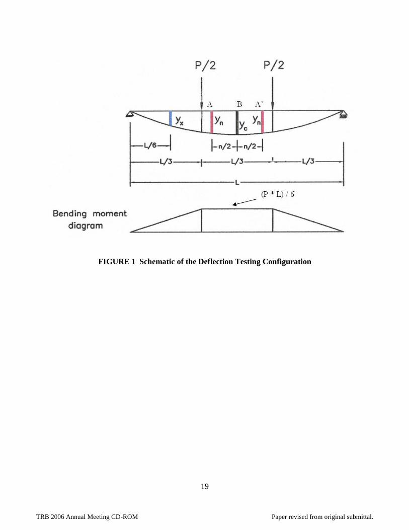
The testing configuration used was different from that recommended by the AASHTO Provisional Standard TP 8-95 [3] and incorporated in the UTM software. The AASHTO Standard estimates the maximum tensile strain at the middle third of the beam from the measured deflection at the mid-span of the beam. For convenience, the UTM testing protocol measures the deflection at 1/6 L (beam span) because it is equal to half the deflection at the mid-span of the beam when the stiffness of the material is uniform along the beam. Both testing configurations do not take into consideration the non-uniform decrease of the stiffness along the beam with the applied cycles, caused by the non-uniformity of the bending moment along the beam. After the


5

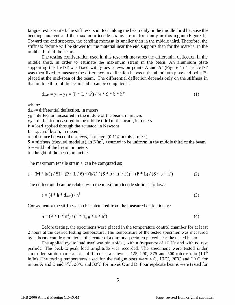
fatigue test is started, the stiffness is uniform along the beam only in the middle third because the bending moment and the maximum tensile strains are uniform only in this region (Figure 1).Toward the end supports, the bending moment is smaller than in the middle third. Therefore, the stiffness decline will be slower for the material near the end supports than for the material in the middle third of the beam.

The testing configuration used in this research measures the differential deflection in the middle third, in order to estimate the maximum strain in the beam. An aluminum plate supporting the LVDT was fixed with glues screws on points A and A’ (Figure 1). The LVDT was then fixed to measure the difference in deflection between the aluminum plate and point B, placed at the mid-span of the beam. The differential deflection depends only on the stiffness in that middle third of the beam and it can be computed as:

dA-B = yB – yA = (P * L * n2) / (4 * S * b * h3) (1)

where:dA-B= differential deflection, in metersyB = deflection measured in the middle of the beam, in metersyA = deflection measured in the middle third of the beam, in metersP = load applied through the actuator, in NewtonsL = span of beam, in metersn = distance between the screws, in meters (0.114 in this project)S = stiffness (flexural modulus), in N/m2, assumed to be uniform in the middle third of the beamb = width of the beam, in metersh = height of the beam, in meters

The maximum tensile strain ε, can be computed as:

ε = (M * h/2) / SI = (P * L / 6) * (h/2) / (S * b * h3 / 12) = (P * L) / (S * b * h2) (2)

The deflection d can be related with the maximum tensile strain as follows:

ε = (4 * h * dA-B) / n2 (3)

Consequently the stiffness can be calculated from the measured deflection as:

S = (P * L * n2) / (4 * dA-B * b * h3) (4)

Before testing, the specimens were placed in the temperature control chamber for at least 2 hours at the desired testing temperature. The temperature of the tested specimen was measuredby a thermocouple mounted at the center of a dummy specimen placed near the tested beam.

The applied cyclic load used was sinusoidal, with a frequency of 10 Hz and with no rest periods. The peak-to-peak load amplitude was recorded. The specimens were tested under controlled strain mode at four different strain levels: 125, 250, 375 and 500 microstrain (10-6 in/in). The testing temperatures used for the fatigue tests were 4oC, 10oC, 20oC and 30oC for mixes A and B and 4oC, 20oC and 30oC for mixes C and D. Four replicate beams were tested for


6

each condition, with a total of 64 beams each for mixes A and B and 48 beams each for mixes Cand D.

The failure of the specimen was considered when the beam reached 50% of the initialstiffness. For mix C, the stiffness after two million cycles did not drop to half of the initial stiffness at any of the strain levels used for Mixes A, B and C. Therefore, the four strain levelsused were: 250, 375, 500 and 625 microstrain (10-6 in/in) for 4oC; 500, 625, 750 and 875 microstrain (10-6 in/in) for 20oC; and 750, 875, 1000 and 1125 microstrain (10-6 in/in) for 30oC. The following data was recorded periodically during the test: test loading time, cycle number, maximum and minimum applied load and deflection, tensile stress, strain, phase angle, flexural stiffness, modulus of elasticity and the dissipated energy.

For all beams tested in this experiment it was observed that the flexural stiffness is decreasing with the increasing of number of loading cycles. The stiffness of some asphalt specimens did not drop to half of the initial stiffness after the maximum number of cycles of 2 million, especially the specimens tested at 250 and 125 microstrain. For these specimens, a linear regression model was developed from the stiffness data recorded between 500,000 and 2,000,000 cycles. The linear model was then used to predict the number of cycles for which the specimen would reach half of the initial stiffness.

It was observed during the fatigue tests that a deviation in the temperature during the testing of ±10C leads to a significant change in the flexural stiffness. A correction procedure was developed in order to correct the flexural stiffness to the desired temperature and was applied to the stiffness data recorded during the test [2]

The average values of the fatigue life at each temperature and strain level is given in Table 2 for each of the four mixes. The data reported in the Table 2 indicate that, as expected, all mixes had a longer fatigue life at lower levels of strain. The temperature, which affected the initial stiffness, influenced the fatigue life of the specimens. The beams tested at 40C and 100C had a longer fatigue life than those tested at 200C and 300C. Mix C, which contained SBS polymer in the binder composition, had the longest fatigue life among the mixes tested in this project.

A linear regression model relating the log of the number of cycles to failure and the tensile strain and the initial stiffness was developed from the measured fatigue lives recorded for the four mixes. The fatigue model has the following form:

log Nf = a + b * (1 / ε) + c * (1 / S) (5) where:Nf = number of cycles to failure (drop in the bending stiffness to 50% of the initial stiffness)ε = tensile strain (mm/mm or in/in)S = initial bending stiffness (MPa) for asphalt beams after temperature correctiona, b, c = experimentally determined coefficients

The coefficients are given in Table 3. The intercept, a, changes if the bending stiffness, S, is measured in MPa or in psi.


7

Dynamic Resilient Modulus Testing and Test Results

The dynamic resilient modulus testing was performed according to standard test method AASHTO TP 62-03 [4] but at different temperatures and loading frequencies. The dynamic modulus test is a cyclic compressive test performed on cylindrical asphalt specimens with thedimensions of 100 mm diameter (4 in.) and 150 mm height (6 in.). The samples were obtained by coring and sawing from 150 mm diameter (6 in.) and 200 mm height (8 in.) HMA cylinders fabricated in the Superpave Gyratory Compactor. The air void content was determined for each sample; the values were between 5.5 and 7.4 percent.

Two LVDTs are mounted on the side of the specimen using a system of screws and nuts glued to the specimen. The axial strain in the central region of the specimen is computed by averaging the deformation recorded by the two LVDTs and dividing it to the gage length (100 mm).

In this test, a sinusoidal axial compressive load is applied to the cylindrical specimen at a sweep of loading frequencies. During testing, the UTM system measures the vertical stress and the resulting vertical compression strain. The dynamic resilient modulus E* is calculated for each load cycle by dividing the peak-to-peak stress to the recoverable strain under a repeated sinusoidal waveform loading. For a given loading frequency, the dynamic resilient modulus is reported as the average value for the last five load cycles at each load frequency.

The asphalt specimens were tested at five temperatures 4oC, 10oC, 20oC, 30oC and 35oC and five load frequencies (10 Hz, 5 Hz, 1 Hz, 0.5 Hz and 0.1 Hz). The specimens were conditioned in the temperature control chamber for at least two hours before testing.

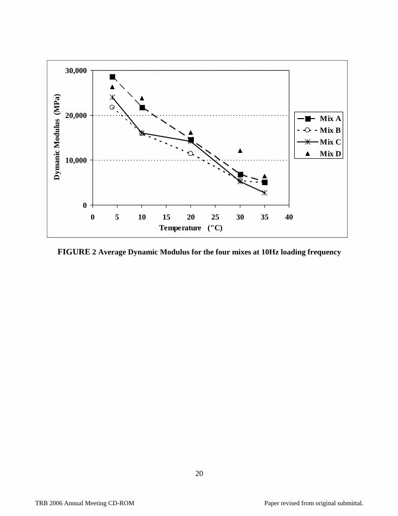
The detailed results of the dynamic modulus tests are provided in reference [2]. For the sake of brevity, only the average values of the dynamic resilient modulus at each temperature and at 10 Hz loading frequency are given in Figure 2. The following conclusions were drawnbased on the results of the dynamic modulus testing [2]:

• Mix D had the highest dynamic modulus, followed by mix A and then by Mixes C and B.• Mix A had a higher dynamic modulus than mix B, proving that the aggregate gradation

and binder content affect the dynamic modulus value. Mix A had different aggregate structure and binder content but the same binder grade as Mix B.

• Mixes B and C had the lowest and quite similar values for the dynamic modulus at all loading frequencies. These two mixes had the same aggregate blend, the same binder content but different binder grades: PG 64-22 (Mix B) and PG 70-28 (Mix C). Mix C contained SBS polymer modified binder. This may indicate that the gradation of the aggregate blend has a higher influence on the dynamic modulus of asphalt concrete than the binder grade, and thus binder viscosity, has.

• For all four mixes and for the range of temperatures used, the loading variable that influenced the most the dynamic modulus was the temperature. A small variation in the testing temperature led to a significant change of the mixes characteristics. In the range of the loading frequency used, the loading frequency was the second most influential factor, followed by the percent air voids in the compacted mix [2].


8

RELATIONS TO THE NCHRP PAVEMENT DESIGN MODEL

The Dynamic Modulus Prediction Model For the structural design of flexible pavements, the accurate prediction of the dynamic modulus of HMA represents a key factor in the, since it has a significant influence on the pavement response. The equation for predicting dynamic modulus included in the NCHRP Design Guide [1], popularly known as the Witczak equation, is:

)log393532.0log313351.0603313.0(34

238384

42

200200

1

]00547.0)(000017.0003958.00021.0871977.3[

)(802208.0

058097.0002841.0)(001767.0029232.0249937.1*log

η−−−++−+−

++

−

−+−+−=

fabeff

beff

a

e

PPPP

VV

V

VPPPE

(6)

where,

E = Asphalt Mix Dynamic Modulus, in 105 psiη = Bitumen viscosity, in 106 poise (at any temperature, degree of aging)f = Load frequency, in HzVa = percent air voids in the mix, by volumeVbeff = effective bitumen content, by volume, in percentP200 = percent passing the No. 200 sieve, by total aggregate weightP34 , P38 , P4 = cumulative percent retained on the ¾ inch sieve, the 3/8 inch sieve and the

No. 4 sieve, by total aggregate weight

The equation was derived based on a database of 2,750 dynamic modulus measurements obtained from 205 different asphalt mixtures [1].

The viscosity of the binder at the temperature for which the dynamic modulus is computed is estimated with the following equation:

log[log(η)] = A + VTS * log(T) (7) where:

η = Bitumen viscosity, in 106 poise (at the desired temperature)T – temperature (in Rankine)

The coefficients of the viscosity model, A and VTS, are determined by regression analysis from binder viscosity data measured at no less than five temperatures. The NCHRP Guide recommends a set of default values of A and VTS for each PG binder grade [1]. The Fatigue Model for HMA mixes

The NCHRP Design Guide [1] contains models for predicting load associated cracking. The Guide assumes that alligator cracks initiate at the bottom of the asphalt concrete layer and then propagate upward. These cracks are named bottom-up fatigue cracks. The NCHRP Guide considers longitudinal cracking in the wheel-path as top-down fatigue cracking. The extend of the bottom –up and top-down cracks are associated with the fatigue damages accumulated at the bottom of asphalt concrete layer and, respectively, the top of the asphalt concrete layer.


9

The NCHRP Design Guide model adopted Miner’s law to estimate fatigue damage:

(8) where,

D = damage.T = total number of periods.ni = actual traffic for period i.Ni = allowable repetitions to failure under conditions prevailing in period i.

The fatigue model used in the design guide obtained by numerical optimization and other modes of comparison is as below:

Nf = 0.00432 * k1’ * C * (1 /εt )3.9492 * (1 / E)1.281 (9)

where:C = 10M and M = 4.84*[Vb / (Va+Vb) – 0.69]

Vb = effective binder volumetric content (%).Va = air voids (%).E = dynamic modulus of HMA, psiεt = tensile strain, in./in.

The parameter k1’ was introduced to account for different asphalt layer thicknesses and is given by below for bottom-up cracking. The parameter k1’ is very close to 250 for asphalt layer thicknesses equal or above five inches, and is given by:

k1’ = 1.0 / {0.000398 + 0.003602 / [1 + e(11.02 – 3.69 * hac) ] } (10)

For top-down cracking, '1k is given by:

k1’ = 1.0 / {0.01 + 12 / [1 + e(15.676 - 2.8186 * hac) ] } (11)

where hac is the thickness of the HMA layer, in inches

COMPARISON BETWEEN THE RESEARCH FINDINGS AND THE MODELS INCLUDED IN THE NCHRP DESIGN GUIDE

Comparison of predicted and measured dynamic modulus for HMA

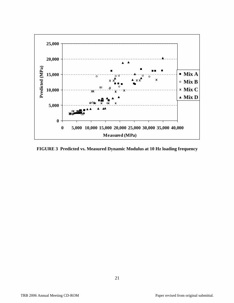
Since the dynamic modulus tests were performed on four representative Kansas Superpave HMA mixes at several temperature and load frequencies, and the composition and volumetric characteristics are known, it is important to compare the measured dynamic moduli with the values predicted by the Witczak equation (Equation 6). For Level 3 design of flexible pavement


10

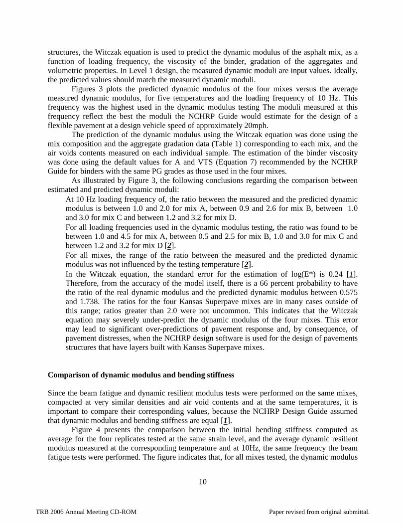
structures, the Witczak equation is used to predict the dynamic modulus of the asphalt mix, as a function of loading frequency, the viscosity of the binder, gradation of the aggregates and volumetric properties. In Level 1 design, the measured dynamic moduli are input values. Ideally, the predicted values should match the measured dynamic moduli.

Figures 3 plots the predicted dynamic modulus of the four mixes versus the average measured dynamic modulus, for five temperatures and the loading frequency of 10 Hz. This frequency was the highest used in the dynamic modulus testing The moduli measured at this frequency reflect the best the moduli the NCHRP Guide would estimate for the design of a flexible pavement at a design vehicle speed of approximately 20mph.

The prediction of the dynamic modulus using the Witczak equation was done using the mix composition and the aggregate gradation data (Table 1) corresponding to each mix, and the air voids contents measured on each individual sample. The estimation of the binder viscosity was done using the default values for A and VTS (Equation 7) recommended by the NCHRP Guide for binders with the same PG grades as those used in the four mixes.

As illustrated by Figure 3, the following conclusions regarding the comparison between estimated and predicted dynamic moduli:• At 10 Hz loading frequency of, the ratio between the measured and the predicted dynamic

modulus is between 1.0 and 2.0 for mix A, between 0.9 and 2.6 for mix B, between 1.0 and 3.0 for mix C and between 1.2 and 3.2 for mix D.

• For all loading frequencies used in the dynamic modulus testing, the ratio was found to be between 1.0 and 4.5 for mix A, between 0.5 and 2.5 for mix B, 1.0 and 3.0 for mix C and between 1.2 and 3.2 for mix D [2].

• For all mixes, the range of the ratio between the measured and the predicted dynamic modulus was not influenced by the testing temperature [2].

• In the Witczak equation, the standard error for the estimation of log(E*) is 0.24 [1]. Therefore, from the accuracy of the model itself, there is a 66 percent probability to have the ratio of the real dynamic modulus and the predicted dynamic modulus between 0.575 and 1.738. The ratios for the four Kansas Superpave mixes are in many cases outside of this range; ratios greater than 2.0 were not uncommon. This indicates that the Witczak equation may severely under-predict the dynamic modulus of the four mixes. This error may lead to significant over-predictions of pavement response and, by consequence, of pavement distresses, when the NCHRP design software is used for the design of pavements structures that have layers built with Kansas Superpave mixes.

Comparison of dynamic modulus and bending stiffness

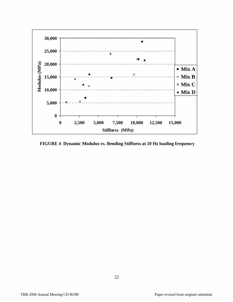
Since the beam fatigue and dynamic resilient modulus tests were performed on the same mixes, compacted at very similar densities and air void contents and at the same temperatures, it is important to compare their corresponding values, because the NCHRP Design Guide assumed that dynamic modulus and bending stiffness are equal [1].

Figure 4 presents the comparison between the initial bending stiffness computed as average for the four replicates tested at the same strain level, and the average dynamic resilient modulus measured at the corresponding temperature and at 10Hz, the same frequency the beam fatigue tests were performed. The figure indicates that, for all mixes tested, the dynamic modulus


11

values are more than two times higher than the bending stiffness. The ratio was the highest for Mix C, which contained polymer modified binder.

It is important to note that, for each beam fatigue test, the initial bending stiffness is the value recorded after 200 cycles of sinusoidal load applications. The initial bending stiffness is always lower that the stiffness measured for the first load application. The dynamic modulus values are recorded for each sample, at each of the five test frequencies, as the average value for the last five of the first 100 cycles of load application. However, the difference in the number of applications for which the modulus and stiffness are recorded cannot explain the large differences between the dynamic modulus and the bending stiffness.

Comparison of fatigue life modelsThe beam fatigue tests conducted in this research allowed the derivation of fatigue life models for each of the four Kansas Superpave mixes studied. A comparison between the life predicted by these models (Equations 3) and the life predicted by the NCHRP fatigue life model (Equation 5) cannot be done in order to determine if the NCHRP model can accurately predict the life of the studied mixes. The comparison is not possible since the two models were not derived in a similar fashion. The NCHRP model was derived from field calibration and numerical optimization and not from laboratory tests.

However, as indicated by the data in Table 2, under identical testing conditions, the laboratory fatigue lives of the four mixtures differed significantly; differences in the fatigue life of the four mixes of one order of magnitude are not uncommon. If the NCHRP fatigue model is used, much smaller differences are expected. The NCHRP model predicts the same fatigue life for mixes B and C because they have almost identical volumetric properties. However, their fatigue lives measured in the laboratory were significantly different; the average fatigue life measured for mix C was approximately 30 times higher than that of mix B. This clearly indicates that a fatigue life model such as that employed in the NCHRP Design Guide cannot represent well the fatigue behavior of all base mixes. A proper fatigue model must incorporate terms that relate the field cracking performance of HMA mixes with their fatigue lives determined in laboratory tests.

CONCLUSIONS AND RECOMMENDATIONS

The objective of this research is to determine the dynamic modulus, the bending stiffness and the fatigue properties of four representative Kansas Superpave HMA mixtures used in theconstruction of base layers for flexible pavements, to allow the development of correlations between the dynamic modulus, stiffness and the fatigue characteristics of typical Superpave Kansas mixtures and to compare the measured dynamic moduli and fatigue life of the Kansas mixes with those predicted by the NCHRP Design Guide.

To achieve these objectives, asphalt concrete beams were tested in third point-bending at constant strain, at four temperatures and four strain levels. Four replicate samples were tested for each condition. Dynamic resilient modulus tests were performed on asphalt cylindrical specimens at five temperatures and five loading frequencies. Four replicate samples were tested for each condition. Multi-linear regression analysis was performed based on the results of the fatigue test and a linear relationship was developed between the bending stiffness and the fatigue


12

life for the asphalt mixes tested. The effects of temperature, loading frequency and air void content on the dynamic resilient modulus were also evaluated with regression analysis.

The following conclusions can be drawn based on the results of this study:1. The dynamic modulus is not a good indicator of the fatigue performance of HMA mixes.

Mix C, which contained binder modified with SBS polymer (PG 70-28), had a much longer fatigue life (Nf) than the mixes with unmodified binder, for all temperatures andstrain levels. At strain values greater than 500 microstrain, the asphalt beams from mixes with unmodified binders couldn’t be tested because the samples broke before 10,000 load cycles, whereas the mix with polymer modified binder (mix C) lasted more than 2 million cycles at strain levels greater than 500 microstrain. However, mix C had very similar dynamic modulus with mix B, which had the same aggregate gradation and volumetric properties but a virgin binder (PG 64-22).

2. In general, the lower the air voids content of the longer the fatigue life, but, due to the small number of specimens tested for each condition and the large variability of fatigue test results, no universal conclusion can be drawn. As expected, all asphalt mixes exhibited a higher dynamic modulus at low temperature that at the high temperatures and,at high loading frequencies than at low frequencies.

3. For all four mixes, the statistical analysis proved that the dynamic resilient modulus significantly decreases when the air void content increases.

4. The measured dynamic moduli on all four mixes were, in most cases, more than two times the dynamic moduli predicted by the Witczak equation, the model included in the NCHRP Design Guide. Therefore, the Witczak equation may severely under-predict the dynamic modulus of the four mixes.

5. At the same temperatures and at the same frequency (10 Hz), the measured dynamic moduli were more than two times larger than the corresponding bending stiffnesses.

6. The laboratory measured fatigue life of the four mixes differed significantly. The fatigue life model included in the NCHRP Design Guide does not reflect these differences. It predicts the same fatigue life for mixes B and C because they have almost identical volumetric properties. However, the laboratory measured fatigue life of mix C was more than one order of magnitude higher than that of mix B.

The following recommendations are made based on the results of this study:• The use of the Witczak equation for prediction of dynamic moduli should be done with

caution. More dynamic moduli tests should be performed to determine if the equation can be used for other mixes or to derive a new equation for dynamic moduli prediction. The test is relatively easy to perform and the cylindrical specimens can be fabricated easily. The dynamic moduli change significantly from one mix to another.

• The fatigue life mode included in the NCHRP Design Guide must be replaced with a model which relates the field cracking performance of HMA mixes with their fatigue lives determined in laboratory tests.

ACKNOWLEDGEMENTS

The authors would like to acknowledge the financial support provided by the Kansas Department of Transportation for this study. The authors acknowledge the cooperation Mr. Chuck Espinosa,


13

from the Material and Research Bureau of the Kansas Department of Transportation, whichhelped with the sample fabrication.


14

REFERENCES

1. NCHRP Guide for Mechanistic-Empirical Design of New and Rehabilitated Pavement Structures. Final Report. NCHRP Project 1-37A. Transportation Research Board, National Research Council, Washington, DC, webdocument: www.trb.org/mepdg/guide.htm Accessed August 2005.

2. Romanoschi, S.A., Dumitru N.I., and Dumitru O., Dynamic Resilient Modulus and the

Fatigue Properties of Kansas HMA Mixes. Final Report. Submitted to the Kansas Department of Transportation, July, 2005.

3. American Association of State Highway and Transportation Officials, “Standard Test Method for Determining the Fatigue Life of Compacted HMA Subjected to Repeated Flexural Bending”, AASHTO Provisional Standard TP 8-95, September 1995.

4. American Association of State Highway and Transportation Officials, “Standard Test

Method for Determining the Dynamic Modulus of Hot-Mix Asphalt Concrete Mixtures”,AASHTO Provisional Standard TP 62-03, July 2003.


15

LIST OF TABLES AND FIGURES

TABLE 1 Aggregate Gradation and Volumetric Properties of the Tested HMA Mixes

TABLE 2 Average Number of Cycles to Failure for the Four HMA Mixes

TABLE 3 Regression Coefficients for the Linear Beam Fatigue Model

FIGURE 1 Schematic of the Deflection Testing Configuration

FIGURE 2 Average Dynamic Modulus for the four mixes at 10Hz loading frequency

FIGURE 3 Predicted vs. Measured Dynamic Modulus at 10 Hz loading frequency

FIGURE 4 Dynamic Modulus vs. Bending Stiffness at 10 Hz loading frequency


16

TABLE 1 Aggregate Gradation and Volumetric Properties of the Tested HMA Mixes

Mix A Mixes B Mix C Mix D ToleranceSieve # Percent Passing

1" 100 100 100 100 100 – 100

3/4" 98 100 100 91 90 – 100

1/2" 89 78 78 73 – 90

3/8" 84 71 71 63#4 66 66 66 56#8 44 45 45 41 35 - 49

#16 30 36 36 32 28 -

#30 19 15 15 24 16 -

#50 10 8 8 16 9 -

#100 6 5 5 8#200 5 2.9 2.9 5.1 2 - 8

Binder Grade PG 64-22 PG 64-22PG 70-28

(SBS polymer modified)

PG 64-22

Asphalt Content (%) 5.20 6.25 6.25 5.1

Gmm 2.445 2.407 2.414 2.561

AV (%) on Beams 5.8 – 9.7 5.2 – 9.4 4.4 – 7.9

AV (%) on Cores 6.5 – 7.3 6.6 – 7.5 6.6 – 7.6


17

TABLE 2 Average Number of Cycles to Failure for the Four HMA Mixes

Temperature (°C)Mix Strain(microstrain) 4 10 20 30

125 17,308,676 12,718,946 6,353,752 8,036,999250 1,014,808 2,142,681 2,045,866 551,406375 74,716 169,961 544,742 343,661

A

500 29,612 39,305 108,368 218,253125 14,163,448 9,289,539 7,128,893 1,481,980250 982,133 1,525,354 1,072,595 256,869375 97,165 129,117 297,763 131,828

B

500 27,186 39,981 44,204 66,723250 9,994,279375 994,924500 151,482 1,340,373625 110,183 2,392,169750 639,668 2,585,640875 371,093 2,597,3611000 1,563,796

C

1125

Not tested at 10°C

911,424125 46,263,326 13,302,418 9,329,610250 2,658,478 2,428,805 3,080,721375 363,180 259,691 1,216,018

D

500 25,725

Not tested at 10°C

78,437 162,445


18

TABLE 3 Regression Coefficients for the Linear Beam Fatigue Model

Mix A Mix B Mix C Mix DLinear Model (Equation 4.2)

If S is in MPa a = -5.401b = 3.641c = 0.4721R2 = 0.821

a = -7.945b = 3.474c = -0.3182R2 = 0.849

a = -2.138b = 4.684c = 2.096R2 = 0.646

a = -6.808b = 3.951c = 0.3486R2 = 0.840

If S is in psi a = -4.381 a = -8.633 a = 2.392 a = -6.055


19

FIGURE 1 Schematic of the Deflection Testing Configuration


20

0

10,000

20,000

30,000

0 5 10 15 20 25 30 35 40Temperature ("C)

Dym

anic

Mod

ulus

(M

Pa)

Mix A

Mix B

Mix C

Mix D

FIGURE 2 Average Dynamic Modulus for the four mixes at 10Hz loading frequency


21

FIGURE 3 Predicted vs. Measured Dynamic Modulus at 10 Hz loading frequency

0

5,000

10,000

15,000

20,000

25,000

0 5,000 10,000 15,000 20,000 25,000 30,000 35,000 40,000

Measured (MPa)

Pre

dict

ed (M

Pa)

Mix AMix BMix CMix D


22

FIGURE 4 Dynamic Modulus vs. Bending Stiffness at 10 Hz loading frequency

0

5,000

10,000

15,000

20,000

25,000

30,000

0 2,500 5,000 7,500 10,000 12,500 15,000

Stiffness (MPa)

Mod

ulus

(MP

a)

Mix AMix BMix CMix D


dynamic resilient modulus and fatigue properties of ...docs.trb.org/prp/06-1012.pdf · 1 06 -1012...

Documents