dynamic programming and markov decision processes - … · linear programming ... dynamic...
TRANSCRIPT
Textbook notes of herd management:Dynamic programming and Markov decision processes
Dina Notat No. 49 August 1996
Anders R. Kristensen1
This report is also available as a PostScript file on World Wide Web at URL:ftp://ftp.dina.kvl.dk/pub/Dina-reports/notatXX.ps
1Dina KVLDept. of Animal Science and Animal HealthRoyal Veterinary and Agricultural UniversityBülowsvej 13DK-1870 Frederiksberg CTel: + 45 35 28 30 91Fax: +45 35 28 30 87E-mail: [email protected]: http://www.dina.kvl.dk/~ark

2 Dina Notat No. 49, August 1996
Contents
1. Introduction. . . . . . . . . . . . . . . . . . . . . . . . . . . . . . . . . . . . . . . . . . . . . . . . . . . 31.1. Historical development. . . . . . . . . . . . . . . . . . . . . . . . . . . . . . . . . . . . . . 31.2. Applications in animal production. . . . . . . . . . . . . . . . . . . . . . . . . . . . . . 4
2. Variability and cyclic production: Markov decision programming. . . . . . . . . . . . . 62.1. Notation and terminology. . . . . . . . . . . . . . . . . . . . . . . . . . . . . . . . . . . . 62.2. A simple dairy cow replacement model. . . . . . . . . . . . . . . . . . . . . . . . . . 62.3. Criteria of optimality . . . . . . . . . . . . . . . . . . . . . . . . . . . . . . . . . . . . . . . 8
2.3.1. Finite planning horizon. . . . . . . . . . . . . . . . . . . . . . . . . . . . . . . . 82.3.2. Infinite planning horizon. . . . . . . . . . . . . . . . . . . . . . . . . . . . . . . 9
2.4. Optimization techniques in general Markov decision programming. . . . . . . 102.4.1. Value iteration. . . . . . . . . . . . . . . . . . . . . . . . . . . . . . . . . . . . . . 102.4.2. The simple dairy model optimized by value iteration. . . . . . . . . . . 112.4.3. Policy iteration. . . . . . . . . . . . . . . . . . . . . . . . . . . . . . . . . . . . . . 132.4.4. Linear programming. . . . . . . . . . . . . . . . . . . . . . . . . . . . . . . . . . 14
2.5. Discussion and applications. . . . . . . . . . . . . . . . . . . . . . . . . . . . . . . . . . 16
3. The curse of dimensionality: Hierarchic Markov processes. . . . . . . . . . . . . . . . . . 173.1. The curse of dimensionality. . . . . . . . . . . . . . . . . . . . . . . . . . . . . . . . . . 173.2. Notation and terminology. . . . . . . . . . . . . . . . . . . . . . . . . . . . . . . . . . . . 193.3. Optimization. . . . . . . . . . . . . . . . . . . . . . . . . . . . . . . . . . . . . . . . . . . . . 223.4. Discussion and applications. . . . . . . . . . . . . . . . . . . . . . . . . . . . . . . . . . 233.5. The numerical example formulated and solved as a hierarchic Markov
process. . . . . . . . . . . . . . . . . . . . . . . . . . . . . . . . . . . . . . . . . . . . . . . . 25
4. Uniformity: Bayesian updating. . . . . . . . . . . . . . . . . . . . . . . . . . . . . . . . . . . . . . 28
5. Herd restraints: Parameter iteration. . . . . . . . . . . . . . . . . . . . . . . . . . . . . . . . . . . 29
6. General discussion. . . . . . . . . . . . . . . . . . . . . . . . . . . . . . . . . . . . . . . . . . . . . . 31
References . . . . . . . . . . . . . . . . . . . . . . . . . . . . . . . . . . . . . . . . . . . . . . . . . . . . . 32
Kristensen: Herd management: Dynamic programming/Markov decision processes 3
1. Introduction
1.1. Historical development
In the late fifties Bellman (1957) published a book entitled"Dynamic Programming". In thebook he presented the theory of a new numerical method for the solution ofsequentialdecision problems. The basic elements of the method are the "Bellman principle of optimality"and functional equations. The idea may be illustrated as follows.
Consider a system being observed over a finite or infinite time horizon split up into periodsor stages. At each stage, thestate of the system is observed, and adecision (or an action)concerning the system has to be made. The decision influences (deterministicly orstochastically) the state to be observed at the next stage, and depending on the state and thedecision made, an immediatereward is gained. The expected total rewards from the presentstage until the end of the planning horizon is expressed by avalue function. The relationbetween the value function at the present stage and the one at the following stage is expressedby the functional equation. Optimal decisions depending on stage and state are determinedbackwards step by step as those maximizing the right hand side of the functional equation.This way of determining an optimalpolicy is based on the Bellman principle of optimalitywhich says: "An optimal policy has the property that whatever the initial state and initialdecision are, the remaining decisions must constitute an optimal policy with regard to the stateresulting from the first decision" (Bellman, 1957 p. 83).
During the following years Bellman published several books on the subject (Bellman, 1961;Bellman and Dreyfus, 1962; Bellman and Kalaba, 1965). The books were very enthusiastic,and the method was expected to be the solution to a very wide range of decision problemsof the real world. The expectations were so great, and they were adduced with such aconviction, that Johnston (1965) ironically compared dynamic programming to a new religion.Others regarded the method as a rather trivial computational device.
Similar stories might be told regarding other new numerical methods, as for instance linearprogramming. However, after some years, the applicational scopes of the methods areencircled. Most often the conclusion is that the method is neither an all-embracing techniquenor a triviality. Between these extremities a rather narrow range of problems remains whereit is a powerful tool. Other problems are, in some cases, not suitable to be solved by themethod. In other cases alternative methods are better.
This also turned out to be the case in dynamic programming. One of the basic elements ofdynamic programming is the sequential approach, which means that it fits sequential decisionproblems best. Obvious examples of sequential decisions in animal production includereplacement of animals (it is relevant to consider at regular time intervals whether the presentasset should be replaced or it should be kept for an additional period), insemination andmedical treatment. Dynamic programming is a relevant tool, but if the traits of the animal arewell defined and their precise behavior over time is known in advance, there are othermethods that might be applied to determine the optimal decisions analytically. On the otherhand, if the traits of the animal are affected byrandom variation over time and among
4 Dina Notat No. 49, August 1996
animals, the decisions will depend on the present observations of the traits. In that casedynamic programming is an obvious technique to be used in the determination of optimaldecisions and policies.
Having identified dynamic programming as a relevant method to be used with sequentialdecision problems in animal production, we shall continue on the historical development. In1960 Howard published a book on "Dynamic Programming and Markov Processes". As willappear from the title, the idea of the book was to combine the dynamic programmingtechnique with the mathematically well established notion of aMarkov chain. A naturalconsequence of the combination was to use the termMarkov decision process to describe thenotion. Howard (1960) also contributed to the solution of infinite stage problems, where thepolicy iteration method was created as an alternative to the stepwise backward contractionmethod, which Howard calledvalue iteration. The policy iteration was a result of theapplication of the Markov chain environment and it was an important contribution to thedevelopment of optimization techniques.
The policy iteration technique was developed for two criteria of optimality, namelymaximization of total expecteddiscounted rewards and maximization of expectedaveragerewards per stage. Later on, Jewell (1963) presented a policy iteration technique for themaximization of average rewards over time forsemi-Markov decision processes, which areMarkov decision processes of which the stage length is a random variable. Howard (1971)presented a value iteration method for semi-Markov decision processes.
For the sake of completeness it should also be mentioned thatlinear programming was earlyidentified as an optimization technique to be applied to Markov decision processes asdescribed by, for instance, Hadley (1964), but no animal production models known to theauthor have applied that technique. This is in accordance with a conclusion of White andWhite (1989) that policy iteration (except in special cases) is more efficient than linearprogramming.
Since the publication of the first mentioned book by Howard (1960) an intensive research inMarkov decision programming has been carried out. Many results have been achievedconcerning the relations between the various optimization techniques and criteria ofoptimality. Reviews of these developments are given by van der Wal and Wessels (1985) aswell as White and White (1989).
1.2. Applications in animal production
The dominant area of application in animal production has been for solving the animalreplacement problem either alone or in connection with insemination and medical treatment.It is however expected that recent methodological developments will broaden the applicationalscope as discussed by Kristensen & Jørgensen (1995).
Already three years after the book by Howard (1960), an application to the dairy cowreplacement problem was published by Jenkins and Halter (1963). Their model only includedthe trait "lactation number" (at 12 levels), and the permanent value of the study was only toillustrate that Markov decision programming is a possible tool to be applied to the problem.
Kristensen: Herd management: Dynamic programming/Markov decision processes 5
A few years later, however, Giaever (1966) published a study which represents a turning-pointin the application of the method to the animal (dairy cow) replacement problem. Heconsidered all three optimization techniques (value iteration, policy iteration and linearprogramming), described how to ensure that all mathematical conditions were satisfied, andpresented an eminent model to describe the production and feed intake of a dairy cow. Thework of Giaever (1966) has not got the credit in literature that it deserves (maybe because itis only available on microfilm). In a review by van Arendonk (1984) it is not even mentioned.
During the following 20 years, several dairy cow replacement models using Markov decisionprogramming were published, but from amethodological point of view none of them havecontributed anything new compared to Giaever (1966). Several studies, however, havecontributed inother ways. Smith (1971) showed that the rather small model of Giaever (1966)with 106 states did not represent the upper limit. His state space included more than 15 000states. Kristensen and Østergaard (1982) as well as van Arendonk (1985; 1986) and vanArendonk and Dijkhuizen (1985) studied the influence of prices and other conditions on theoptimal replacement policy. Other studies (Killen and Kearney, 1978; Reenberg, 1979) hardlyreached the level of Jenkins and Halter (1963). Even though the sow replacement problem isalmost identical to that of dairy cows, very few studies on sows have been published. Theonly exceptions known to the author are Huirne (1990) and Jørgensen (1992).
A study by Ben-Ari et al. (1983) deserves special attention. As regards methodology it is notremarkable, but in that study the main difficulties concerning application to animal productionmodels were identified and clearly formulated. Three features were mentioned:
1) Uniformity. The traits of an animal are difficult to define and measure. Furthermore therandom variation of each trait is relatively large.
2) Reproductive cycle. The production of an animal is cyclic. It has to be decidedin whichcycle to replace as well aswhen to replace inside a cycle.
3) Availability. Only a limited supply of replacements (in that case heifers) is available.
The first feature in fact covers two different aspects, namelyuniformity because the traits aredifficult to define and measure, andvariability because the traits vary at random amonganimals and over time. The third feature is an example of aherd restraint, i.e. a restrictionthat applies to the herd as a whole and not to the individual animal. Other examples of herdrestraints are a production quota or a limited housing capacity. We shall therefore considerthe more general problem of herd restraints.
We may conclude that until the mid-eighties, the methodological level concerning theapplication of Markov decision programming to animal production models was representedby Giaever (1966). The main difficulties that the method should overcome had been identifiedby Ben-Ari et al. (1983). If we compare the approach of Giaever (1966) to the difficulties thatit ought to solve, we may conclude that the problems related tovariability are directly solved,and as it has been shown by Kristensen and Østergaard (1982) as well as van Arendonk(1985), the problems concerning thecyclic production may readily be solved without anymethodological considerations. The only problem concerning variability and cyclic productionis that in order to cover the variability, the state variables (traits) have to be represented bymany levels, and to deal with the cyclic production a state variable representing the stage of
6 Dina Notat No. 49, August 1996
the cycle has to be included. Both aspects contributes significantly to an explosive growth ofthe state space. We therefore face adimensionality problem. Even though all necessaryconditions of a Markov decision process are met, the solution in practice is prohibitive evenon modern computers. The problems concerning uniformity and herd restraints arenot solvedby the approach of Giaever (1966).
2. Variability and cyclic production: Markov decision programming
As mentioned in the introduction, Markov decision programming is directly able to take thevariability in traits and the cyclic production into account without any adaptations. In orderto have a frame of reference, we shall briefly present the theory of traditional Markovdecision programming originally described by Howard (1960).
2.1. Notation and terminology
Consider a discrete time Markov decision process with a finitestate spaceU = 1,2,...,u anda finite action setD. A policy s is a map assigning to each statei an actions(i) ∈ D. Let pij
d
be thetransition probability from statei to statej if the actiond ∈ D is taken. Therewardto be gained when the statei is observed, and the actiond is taken, is denoted asri
d. The timeinterval between two transitions is called astage.
We have now defined the elements of a traditional Markov decision process, but in somemodels we further assume that if statei is observed, and actiond is taken, a physical quantityof mi
d is involved (e.g. Kristensen, 1989; 1991). In this study we shall refer tomid as the
physical output. If s(i) = d, the symbolsrid, mi
d and pijd are also written asri
s, mis and pij
s,respectively.
An optimal policy is defined as a policy that maximizes (or minimizes) some predefinedobjective function. The optimization technique (i.e. the method to identify an optimal policy)depends on the form of the objective function or - in other words - on the criterion ofoptimality. The over-all objective to maximize net revenue of the entire herd may (dependingon the circumstances) result in different criteria of optimality formulated as alternativeobjective functions. The choice of criterion depends on whether the planning horizon is finiteor infinite.
2.2. A simple dairy cow replacement model
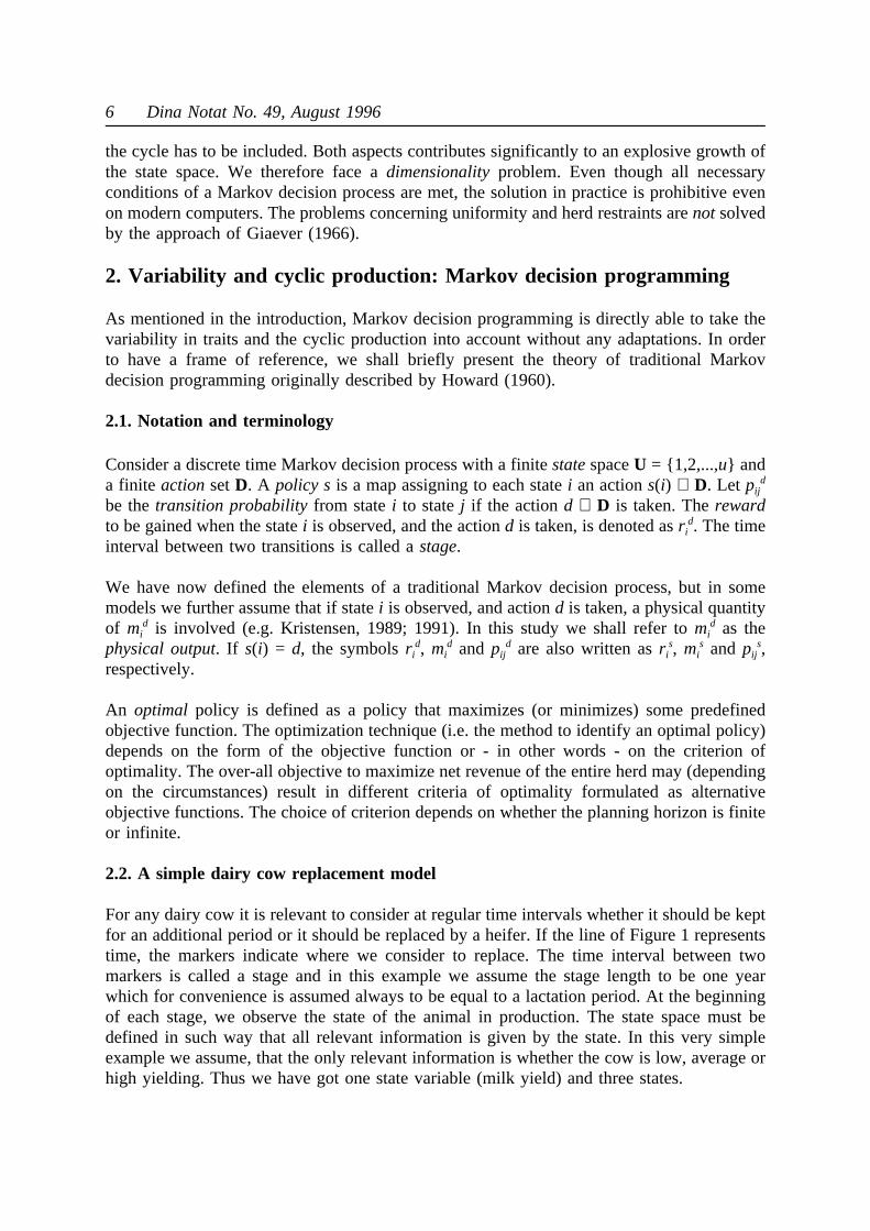
For any dairy cow it is relevant to consider at regular time intervals whether it should be keptfor an additional period or it should be replaced by a heifer. If the line of Figure 1 representstime, the markers indicate where we consider to replace. The time interval between twomarkers is called a stage and in this example we assume the stage length to be one yearwhich for convenience is assumed always to be equal to a lactation period. At the beginningof each stage, we observe the state of the animal in production. The state space must bedefined in such way that all relevant information is given by the state. In this very simpleexample we assume, that the only relevant information is whether the cow is low, average orhigh yielding. Thus we have got one state variable (milk yield) and three states.
Kristensen: Herd management: Dynamic programming/Markov decision processes 7
Having observed the state, we have to take an action concerning the cow. We assume that the
Figure 1. Stages of a Markov decision process.
action is either to keep the cow for at least an additional stage or to replace it by a heifer atthe end of the stage.
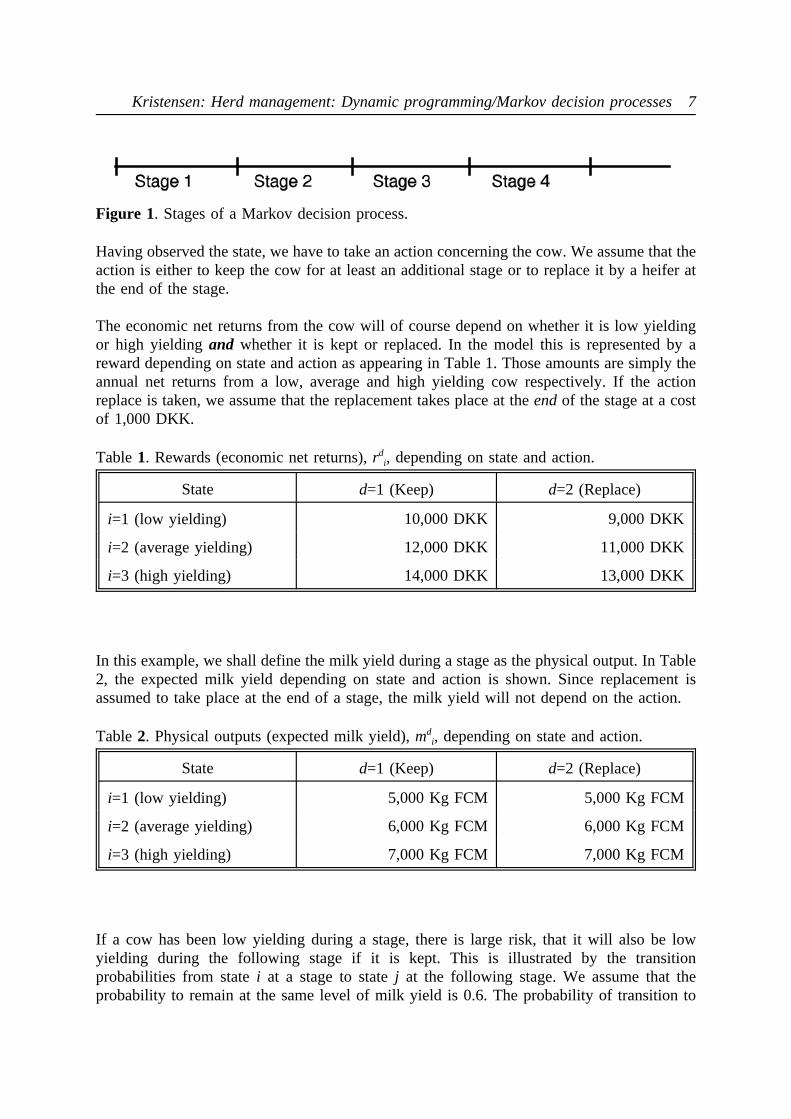
The economic net returns from the cow will of course depend on whether it is low yieldingor high yieldingand whether it is kept or replaced. In the model this is represented by areward depending on state and action as appearing in Table 1. Those amounts are simply theannual net returns from a low, average and high yielding cow respectively. If the actionreplace is taken, we assume that the replacement takes place at theend of the stage at a costof 1,000 DKK.
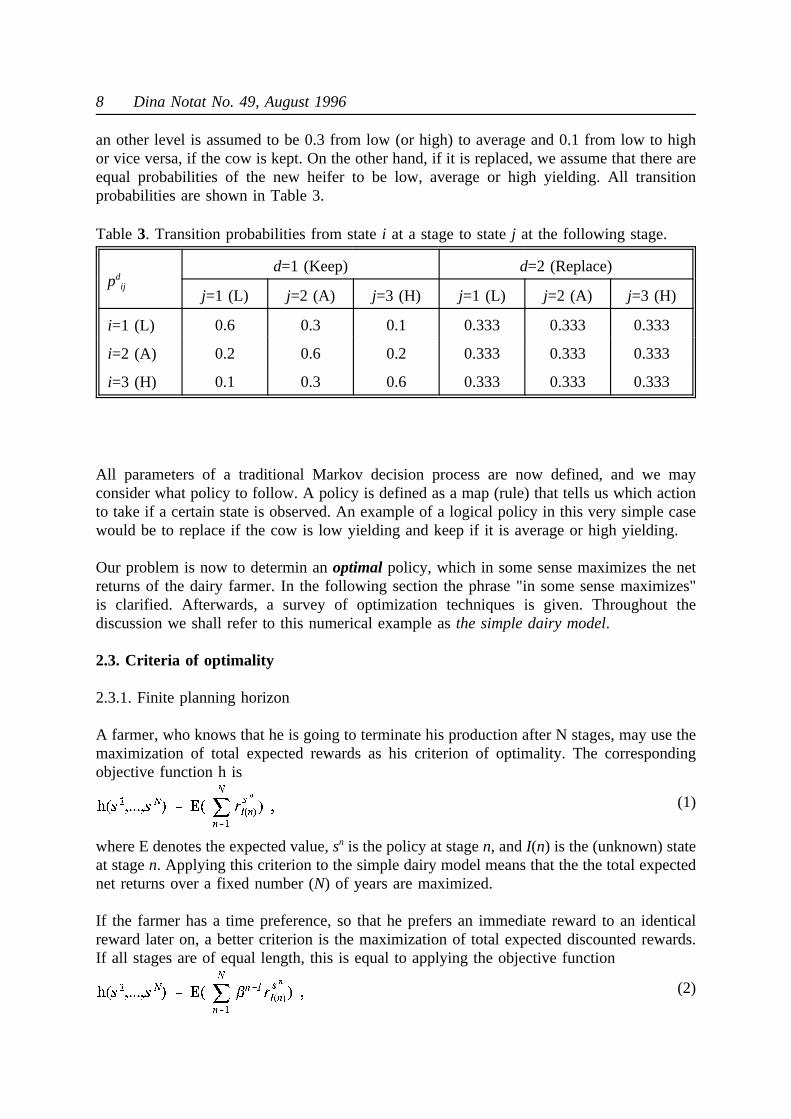
In this example, we shall define the milk yield during a stage as the physical output. In Table
Table1. Rewards (economic net returns),rdi, depending on state and action.
State d=1 (Keep) d=2 (Replace)
i=1 (low yielding) 10,000 DKK 9,000 DKK
i=2 (average yielding) 12,000 DKK 11,000 DKK
i=3 (high yielding) 14,000 DKK 13,000 DKK
2, the expected milk yield depending on state and action is shown. Since replacement isassumed to take place at the end of a stage, the milk yield will not depend on the action.
If a cow has been low yielding during a stage, there is large risk, that it will also be low
Table2. Physical outputs (expected milk yield),mdi, depending on state and action.
State d=1 (Keep) d=2 (Replace)
i=1 (low yielding) 5,000 Kg FCM 5,000 Kg FCM
i=2 (average yielding) 6,000 Kg FCM 6,000 Kg FCM
i=3 (high yielding) 7,000 Kg FCM 7,000 Kg FCM
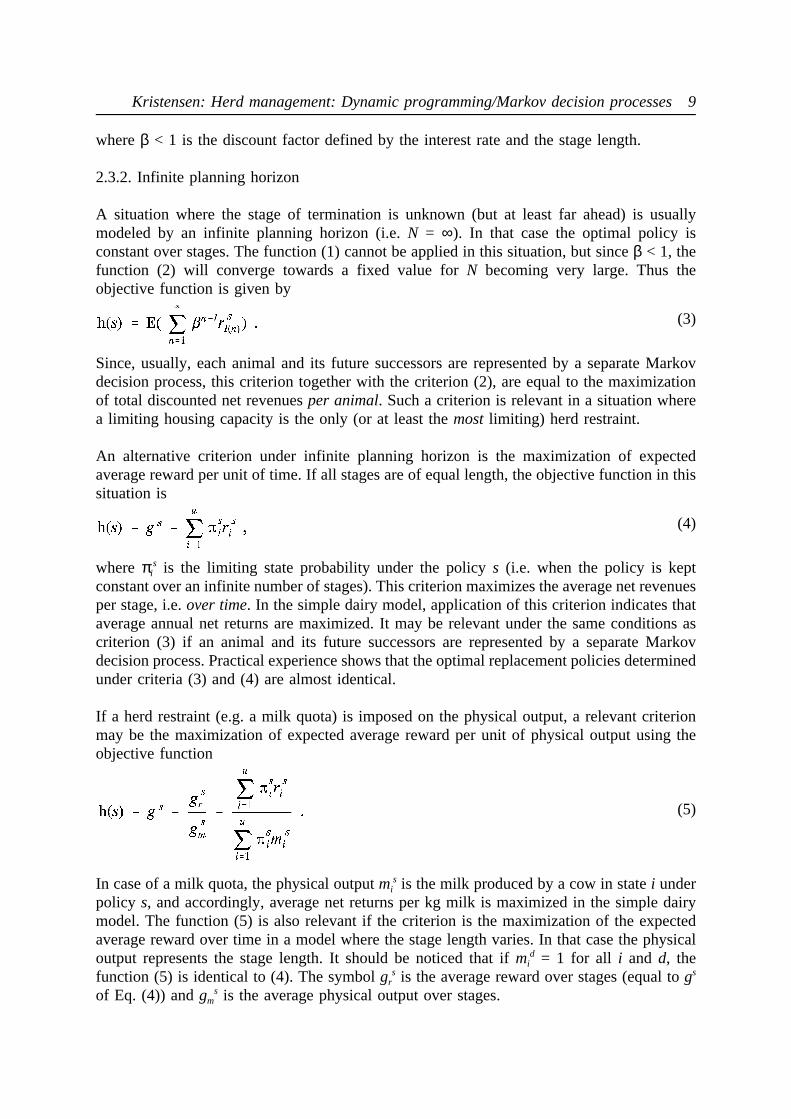
yielding during the following stage if it is kept. This is illustrated by the transitionprobabilities from statei at a stage to statej at the following stage. We assume that theprobability to remain at the same level of milk yield is 0.6. The probability of transition to
8 Dina Notat No. 49, August 1996
an other level is assumed to be 0.3 from low (or high) to average and 0.1 from low to highor vice versa, if the cow is kept. On the other hand, if it is replaced, we assume that there areequal probabilities of the new heifer to be low, average or high yielding. All transitionprobabilities are shown in Table 3.
All parameters of a traditional Markov decision process are now defined, and we may
Table3. Transition probabilities from statei at a stage to statej at the following stage.
pdij
d=1 (Keep) d=2 (Replace)
j=1 (L) j=2 (A) j=3 (H) j=1 (L) j=2 (A) j=3 (H)
i=1 (L) 0.6 0.3 0.1 0.333 0.333 0.333
i=2 (A) 0.2 0.6 0.2 0.333 0.333 0.333
i=3 (H) 0.1 0.3 0.6 0.333 0.333 0.333
consider what policy to follow. A policy is defined as a map (rule) that tells us which actionto take if a certain state is observed. An example of a logical policy in this very simple casewould be to replace if the cow is low yielding and keep if it is average or high yielding.
Our problem is now to determin anoptimal policy, which in some sense maximizes the netreturns of the dairy farmer. In the following section the phrase "in some sense maximizes"is clarified. Afterwards, a survey of optimization techniques is given. Throughout thediscussion we shall refer to this numerical example asthe simple dairy model.
2.3. Criteria of optimality
2.3.1. Finite planning horizon
A farmer, who knows that he is going to terminate his production after N stages, may use themaximization of total expected rewards as his criterion of optimality. The correspondingobjective function h is
where E denotes the expected value,sn is the policy at stagen, andI(n) is the (unknown) state
(1)
at stagen. Applying this criterion to the simple dairy model means that the the total expectednet returns over a fixed number (N) of years are maximized.
If the farmer has a time preference, so that he prefers an immediate reward to an identicalreward later on, a better criterion is the maximization of total expected discounted rewards.If all stages are of equal length, this is equal to applying the objective function
(2)
Kristensen: Herd management: Dynamic programming/Markov decision processes 9
whereβ < 1 is the discount factor defined by the interest rate and the stage length.
2.3.2. Infinite planning horizon
A situation where the stage of termination is unknown (but at least far ahead) is usuallymodeled by an infinite planning horizon (i.e.N = ∞). In that case the optimal policy isconstant over stages. The function (1) cannot be applied in this situation, but sinceβ < 1, thefunction (2) will converge towards a fixed value forN becoming very large. Thus theobjective function is given by
Since, usually, each animal and its future successors are represented by a separate Markov
(3)
decision process, this criterion together with the criterion (2), are equal to the maximizationof total discounted net revenuesper animal. Such a criterion is relevant in a situation wherea limiting housing capacity is the only (or at least themost limiting) herd restraint.
An alternative criterion under infinite planning horizon is the maximization of expectedaverage reward per unit of time. If all stages are of equal length, the objective function in thissituation is
where πis is the limiting state probability under the policys (i.e. when the policy is kept
(4)
constant over an infinite number of stages). This criterion maximizes the average net revenuesper stage, i.e.over time. In the simple dairy model, application of this criterion indicates thataverage annual net returns are maximized. It may be relevant under the same conditions ascriterion (3) if an animal and its future successors are represented by a separate Markovdecision process. Practical experience shows that the optimal replacement policies determinedunder criteria (3) and (4) are almost identical.
If a herd restraint (e.g. a milk quota) is imposed on the physical output, a relevant criterionmay be the maximization of expected average reward per unit of physical output using theobjective function
In case of a milk quota, the physical outputmis is the milk produced by a cow in statei under
(5)
policy s, and accordingly, average net returns per kg milk is maximized in the simple dairymodel. The function (5) is also relevant if the criterion is the maximization of the expectedaverage reward over time in a model where the stage length varies. In that case the physicaloutput represents the stage length. It should be noticed that ifmi
d = 1 for all i and d, thefunction (5) is identical to (4). The symbolgr
s is the average reward over stages (equal togs
of Eq. (4)) andgms is the average physical output over stages.
10 Dina Notat No. 49, August 1996
2.4. Optimization techniques in general Markov decision programming
2.4.1. Value iteration
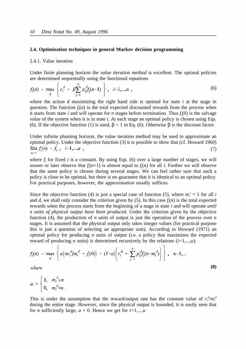
Under finite planning horizon thevalue iteration method is excellent. The optimal policiesare determined sequentially using the functional equations
where the actiond maximizing the right hand side is optimal for statei at the stage in
(6)
question. The functionfi(n) is the total expected discounted rewards from the process whenit starts from statei and will operate forn stages before termination. Thusfi(0) is the salvagevalue of the system when it is in statei. At each stage an optimal policy is chosen using Eqs.(6). If the objective function (1) is used,β = 1 in Eq. (6). Otherwiseβ is the discount factor.
Under infinite planning horizon, the value iteration method may be used to approximate anoptimal policy. Under the objective function (3) it is possible to show that (cf. Howard 1960)
wherefi for fixed i is a constant. By using Eqs. (6) over a large number of stages, we will
(7)
sooner or later observe thatfi(n+1) is almost equal tofi(n) for all i. Further we will observethat the same policy is chosen during several stages. We can feel rather sure that such apolicy is close to be optimal, but there is no guarantee that it is identical to an optimal policy.For practical purposes, however, the approximation usually suffices.
Since the objective function (4) is just a special case of function (5), wheremis = 1 for all i
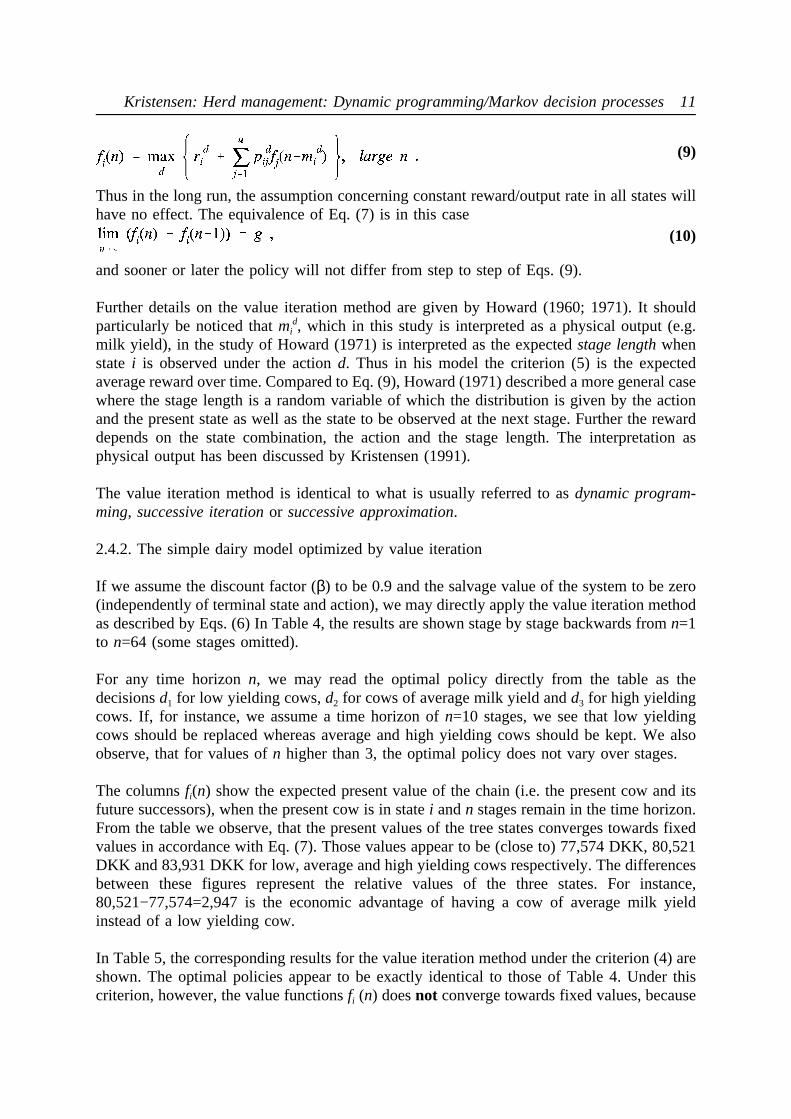
andd, we shall only consider the criterion given by (5). In this casefi(n) is the total expectedrewards when the process starts from the beginning of a stage in statei and will operateuntiln units of physical output have been produced. Under the criterion given by the objectivefunction (4), the production ofn units of output is just the operation of the process overnstages. It is assumed that the physical output only takes integer values (for practical purposethis is just a question of selecting an appropriate unit). According to Howard (1971) anoptimal policy for producingn units of output (i.e. a policy that maximizes the expectedreward of producingn units) is determined recursively by the relations (i=1,...,u):
This is under the assumption that the reward/output rate has the constant value ofrid/mi
d
(8)
during the entire stage. However, since the physical output is bounded, it is easily seen thatfor n sufficiently large,a = 0. Hence we get fori=1,...,u
Kristensen: Herd management: Dynamic programming/Markov decision processes 11
Thus in the long run, the assumption concerning constant reward/output rate in all states will
(9)
have no effect. The equivalence of Eq. (7) is in this case
and sooner or later the policy will not differ from step to step of Eqs. (9).
(10)
Further details on the value iteration method are given by Howard (1960; 1971). It shouldparticularly be noticed thatmi
d, which in this study is interpreted as a physical output (e.g.milk yield), in the study of Howard (1971) is interpreted as the expectedstage length whenstatei is observed under the actiond. Thus in his model the criterion (5) is the expectedaverage reward over time. Compared to Eq. (9), Howard (1971) described a more general casewhere the stage length is a random variable of which the distribution is given by the actionand the present state as well as the state to be observed at the next stage. Further the rewarddepends on the state combination, the action and the stage length. The interpretation asphysical output has been discussed by Kristensen (1991).
The value iteration method is identical to what is usually referred to asdynamic program-ming, successive iteration or successive approximation.
2.4.2. The simple dairy model optimized by value iteration
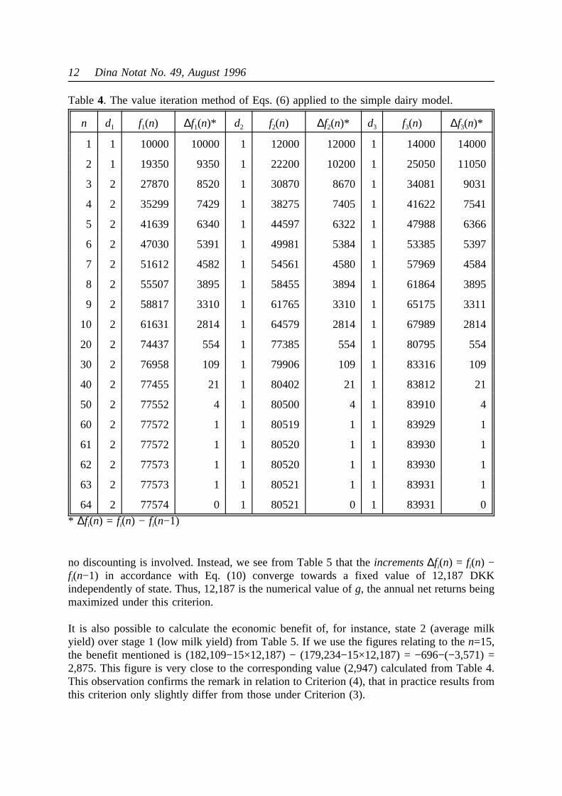
If we assume the discount factor (β) to be 0.9 and the salvage value of the system to be zero(independently of terminal state and action), we may directly apply the value iteration methodas described by Eqs. (6) In Table 4, the results are shown stage by stage backwards fromn=1to n=64 (some stages omitted).
For any time horizonn, we may read the optimal policy directly from the table as thedecisionsd1 for low yielding cows,d2 for cows of average milk yield andd3 for high yieldingcows. If, for instance, we assume a time horizon ofn=10 stages, we see that low yieldingcows should be replaced whereas average and high yielding cows should be kept. We alsoobserve, that for values ofn higher than 3, the optimal policy does not vary over stages.
The columnsfi(n) show the expected present value of the chain (i.e. the present cow and itsfuture successors), when the present cow is in statei andn stages remain in the time horizon.From the table we observe, that the present values of the tree states converges towards fixedvalues in accordance with Eq. (7). Those values appear to be (close to) 77,574 DKK, 80,521DKK and 83,931 DKK for low, average and high yielding cows respectively. The differencesbetween these figures represent the relative values of the three states. For instance,80,521−77,574=2,947 is the economic advantage of having a cow of average milk yieldinstead of a low yielding cow.
In Table 5, the corresponding results for the value iteration method under the criterion (4) areshown. The optimal policies appear to be exactly identical to those of Table 4. Under thiscriterion, however, the value functionsfi (n) doesnot converge towards fixed values, because
12 Dina Notat No. 49, August 1996
no discounting is involved. Instead, we see from Table 5 that theincrements ∆fi(n) = fi(n) −
Table4. The value iteration method of Eqs. (6) applied to the simple dairy model.
n d1 f1(n) ∆f1(n)* d2 f2(n) ∆f2(n)* d3 f3(n) ∆f3(n)*
1 1 10000 10000 1 12000 12000 1 14000 14000
2 1 19350 9350 1 22200 10200 1 25050 11050
3 2 27870 8520 1 30870 8670 1 34081 9031
4 2 35299 7429 1 38275 7405 1 41622 7541
5 2 41639 6340 1 44597 6322 1 47988 6366
6 2 47030 5391 1 49981 5384 1 53385 5397
7 2 51612 4582 1 54561 4580 1 57969 4584
8 2 55507 3895 1 58455 3894 1 61864 3895
9 2 58817 3310 1 61765 3310 1 65175 3311
10 2 61631 2814 1 64579 2814 1 67989 2814
20 2 74437 554 1 77385 554 1 80795 554
30 2 76958 109 1 79906 109 1 83316 109
40 2 77455 21 1 80402 21 1 83812 21
50 2 77552 4 1 80500 4 1 83910 4
60 2 77572 1 1 80519 1 1 83929 1
61 2 77572 1 1 80520 1 1 83930 1
62 2 77573 1 1 80520 1 1 83930 1
63 2 77573 1 1 80521 1 1 83931 1
64 2 77574 0 1 80521 0 1 83931 0
* ∆fi(n) = fi(n) − fi(n−1)
fi(n−1) in accordance with Eq. (10) converge towards a fixed value of 12,187 DKKindependently of state. Thus, 12,187 is the numerical value ofg, the annual net returns beingmaximized under this criterion.
It is also possible to calculate the economic benefit of, for instance, state 2 (average milkyield) over stage 1 (low milk yield) from Table 5. If we use the figures relating to then=15,the benefit mentioned is (182,109−15×12,187) − (179,234−15×12,187) = −696−(−3,571) =2,875. This figure is very close to the corresponding value (2,947) calculated from Table 4.This observation confirms the remark in relation to Criterion (4), that in practice results fromthis criterion only slightly differ from those under Criterion (3).

Kristensen: Herd management: Dynamic programming/Markov decision processes 13
2.4.3. Policy iteration
Table5. The value iteration method of Eqs. (9) applied to the simple dairy model.
n d1 f1(n) ∆f1(n)* d2 f2(n) ∆f2(n)* d3 f3(n) ∆f3(n)*
1 1 10000 10000 1 12000 12000 1 14000 14000
2 1 21000 11000 1 24000 12000 1 27000 13000
3 2 33000 12000 1 36000 12000 1 39500 12500
4 2 45167 12167 1 48100 12100 1 51800 12300
5 2 57355 12189 1 60253 12153 1 64027 12227
6 2 69545 12190 1 72428 12175 1 76228 12201
7 2 81734 12189 1 84612 12183 1 88420 12192
8 2 93922 12188 1 96798 12186 1 100609 12189
9 2 106109 12188 1 108985 12187 1 112797 12188
10 2 118297 12188 1 121172 12187 1 124984 12188
11 2 130484 12187 1 133359 12187 1 137172 12188
12 2 142672 12187 1 145547 12187 1 149359 12188
13 2 154859 12187 1 157734 12187 1 161547 12187
14 2 167047 12187 1 169922 12187 1 173734 12187
15 2 179234 12187 1 182109 12187 1 185922 12187
* ∆fi(n) = fi(n) − fi(n−1)
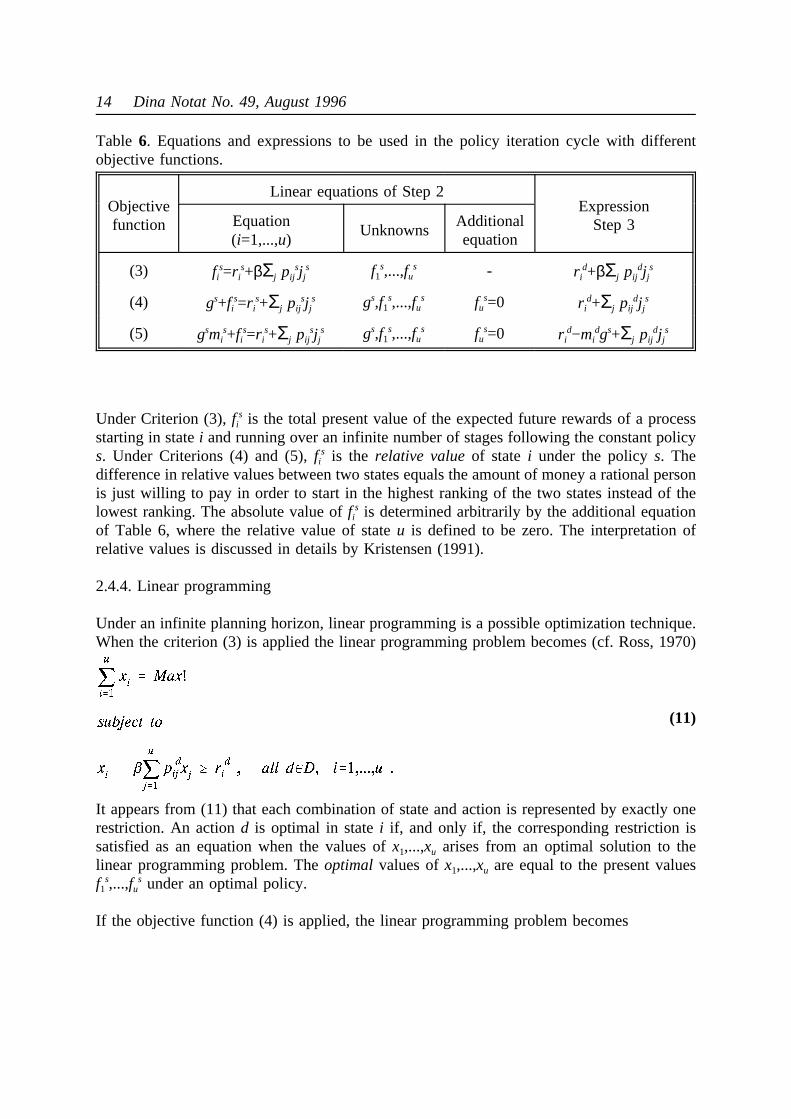
Under infinite planning horizon, thepolicy iteration method may be applied. Unlike the valueiteration method it always provides an optimal policy. It covers all three objective functions(3), (4) and (5). The iteration cycle used for optimization has the following steps:
1) Choose an arbitrary policy s. Go to 2.2) Solve the set of linear simultaneous equations appearing in Table 6. Go to 3.3) For each statei, find the actiond’ that maximizes the expression given in Table 6, and
put s’(i)=d’. If s’=s then stop, since an optimal policy is found. Otherwise redefinesaccording to the new policy (i.e. puts=s’) and go back to 2.
From the equations and expressions of Table 6, we see that also with the policy iterationmethod the objective function (4) is just a special case of (5) wheremi
s = 1 for all i andd.For the objective functions (3) and (4) the policy iteration method was developed by Howard(1960), and for the function (5) a policy iteration method was presented by Jewell (1963).Like Howard (1971), Jewell interpretedmi
d as the expected stage length.
14 Dina Notat No. 49, August 1996
Under Criterion (3),fis is the total present value of the expected future rewards of a process
Table 6. Equations and expressions to be used in the policy iteration cycle with differentobjective functions.
Objectivefunction
Linear equations of Step 2Expression
Step 3Equation(i=1,...,u)
UnknownsAdditionalequation
(3) fis=ri
s+βΣj pijsjj
s f1s,...,fu
s - rid+βΣj pij
djjs
(4) gs+fis=ri
s+Σj pijsjj
s gs,f1s,...,fu
s fus=0 ri
d+Σj pijdjj
s
(5) gsmis+fi
s=ris+Σj pij
sjjs gs,f1
s,...,fus fu
s=0 rid−mi
dgs+Σj pijdjj
s
starting in statei and running over an infinite number of stages following the constant policys. Under Criterions (4) and (5),fi
s is the relative value of state i under the policys. Thedifference in relative values between two states equals the amount of money a rational personis just willing to pay in order to start in the highest ranking of the two states instead of thelowest ranking. The absolute value offi
s is determined arbitrarily by the additional equationof Table 6, where the relative value of stateu is defined to be zero. The interpretation ofrelative values is discussed in details by Kristensen (1991).
2.4.4. Linear programming
Under an infinite planning horizon, linear programming is a possible optimization technique.When the criterion (3) is applied the linear programming problem becomes (cf. Ross, 1970)
It appears from (11) that each combination of state and action is represented by exactly one
(11)
restriction. An actiond is optimal in statei if, and only if, the corresponding restriction issatisfied as an equation when the values ofx1,...,xu arises from an optimal solution to thelinear programming problem. Theoptimal values ofx1,...,xu are equal to the present valuesf1
s,...,fus under an optimal policy.
If the objective function (4) is applied, the linear programming problem becomes

Kristensen: Herd management: Dynamic programming/Markov decision processes 15
In this case an actiond is optimal in statei if and only if xid from the optimal solution is
(12)
strictly positive. The optimal value of the objective function is equal to the average rewardsper stage under an optimal policy. The optimal value ofd∈ D xi
d is equal to the limiting stateprobability πi under an optimal policy.
Using Criterion (5), we may solve the following linear programming problem (cf.Kennedy,1986):
wherea is a pre-determined relative value of stateu chosen sufficiently large to ensure that
(13)
all other relative values are positive. The optimal value of the objective function of the linearprogramming problem is equal to the expected average reward per unit of output as definedin Eq. (5) under an optimal policy. The optimal values of the variablesx1,...,xu-1 are equal tothe relative values of the states 1,...,u-1, provided that the relative value of stateu is equal toa . As it appears, each combination of state and action is represented by one and only onerestriction. An action is optimal in a state if and only if the corresponding restriction issatisfied as an equation in the optimal solution.
Since Criterion (4) is just a special case of (5) with all physical outputs set to the value 1, thelinear programming problem (13) may also be used in the determination of an optimal policyunder Criterion (4).
16 Dina Notat No. 49, August 1996
2.5. Discussion and applications
Under finite planning horizon, the value iteration method is perfect, but in herd managementmodels the planning horizon is rarely well defined. Most often the process is assumed tooperate over an unknown period of time with no pre-determined stage of termination. In suchcases the abstraction of an infinite planning horizon seems more relevant. Therefore we shallpay specific attention to the optimization problem under the criteria (3), (4) and (5) where allthree techniques described in the previous sections are available.
The value iteration method is not exact, and the convergence is rather slow. On the otherhand, the mathematical formulation is very simple, and the method makes it possible tohandle very large models with thousands of states. Further it is possible to let the rewardand/or the physical output depend on the stage number in some pre-defined way. This hasbeen mentioned by van Arendonk (1984) as an advantage in modelling genetic improvementover time. The method has been used in a lot of dairy cow replacement models as anapproximation to the infinite stage optimum. Thus it has been used by Jenkins and Halter(1963), Giaever (1966), Smith (1971), McArthur (1973), Steward et al. (1977; 1978), Killenand Kearney (1978), Ben-Ari et al. (1983), van Arendonk (1985; 1986), van Arendonk andDijkhuizen (1985) and DeLorenzo et al. (1992). Some of the models mentioned have beenvery large. For instance, the model of van Arendonk and Dijkhuizen contained 174 000 states(reported by van Arendonk, 1988). In sows, the method has been used by Huirne et al.(1988).
The policy iteration method has almost exactly the opposite characteristics of the valueiteration method. Because of the more complicated mathematical formulation involvingsolution of large systems of simultaneous linear equations, the method can only handle rathersmall models with, say, a few hundred states. The solution of the linear equations implies theinversion of a matrix of the dimensionu × u , which is rather complicated. On the otherhand, the method is exact and very efficient in the sense of fast convergence. The rewardsare not allowed to depend on the stage except for a fixed rate of annual increase (e.g.inflation) or decrease. However, a seasonal variation in rewards or physical outputs is easilymodeled by including a state variable describing season (each state is usually defined by thevalue of a number of state variables describing the system).
An advantage of the policy iteration method is that the equations in Table 1 aregeneral.Under any policys we are able to calculate directly the economic consequences of followingthe policy by solution of the equations. This makes it possible to compare the economicconsequences of various non-optimal policies to those of the optimal. Further we may use theequations belonging to the criterion (5) to calculate the long run technical results under agiven policy by redefiningri
s andmis . If for instanceri
s = 1 if a calving takes place and zerootherwise, andmi
s is the stage length when statei is observed under policys , thengs, whichis the average number of calvings per cow per year, may be determined from the equations.Further examples are discussed by Kristensen (1991). For an example where the equations areused for calculation of the economic value of culling information, reference is made toKristensen and Thysen (1991).
The policy iteration method has been used by Reenberg (1979) and Kristensen and Østergaard
Kristensen: Herd management: Dynamic programming/Markov decision processes 17
(1982). The models were very small, containing only 9 and 177 states, respectively.
3. The curse of dimensionality: Hierarchic Markov processes
In order to combine the computational advantages of the value iteration method with theexactness and efficiency of the policy iteration method Kristensen (1988; 1991) introduceda new notion of a hierarchic Markov process. It is a contribution to the solution of theproblem referred to as the "curse of dimensionality" since it makes it possible to give exactsolutions to models with even very large state spaces.
3.1. The curse of dimensionality
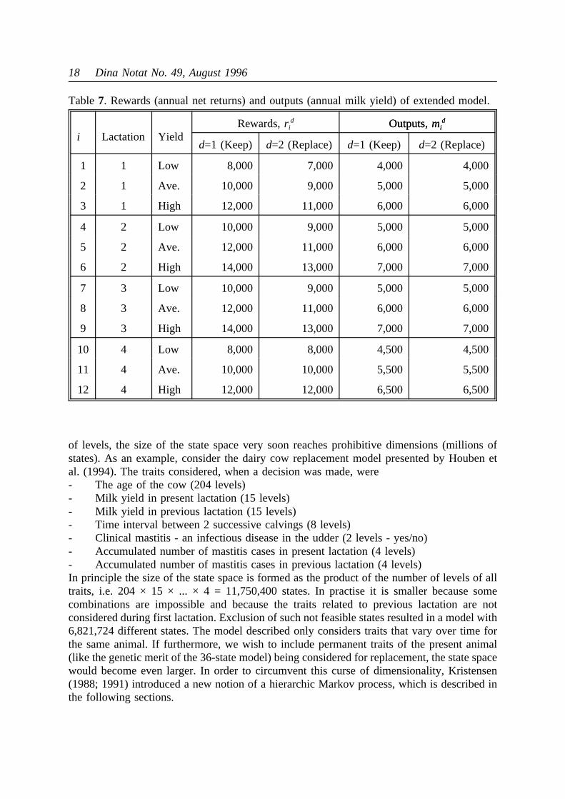
In order to illustrate how the curse of dimensionality arises, we shall reexamine the simpledairy model used in the previous sections. First we shall realize that theage of the animal isnot represented. Thus, if a cow remains high yielding it will never be replaced according tothe optimal policies shown in Tables 4 and 5. This is certainly not realistic, and furthermore,the milk yield also depends on the lactation number. In order to account for age we shallintroduce an additional state variable representing the lactation number of the cow. Forconvenience, we shall assume that the new variable may take the values 1, 2, 3 or 4indicating that the maximum age of a cow in this (still very simple) model is assumed to be4 lactations.
The milk yields (i.e. outputsmid) and economic net returns (i.e. rewardsri
d) assumed for thisslightly extended model appear in Table 7. Because a cow is always replaced after 4lactations, the rewards are identical under both actions for those states representing 4thlactation.
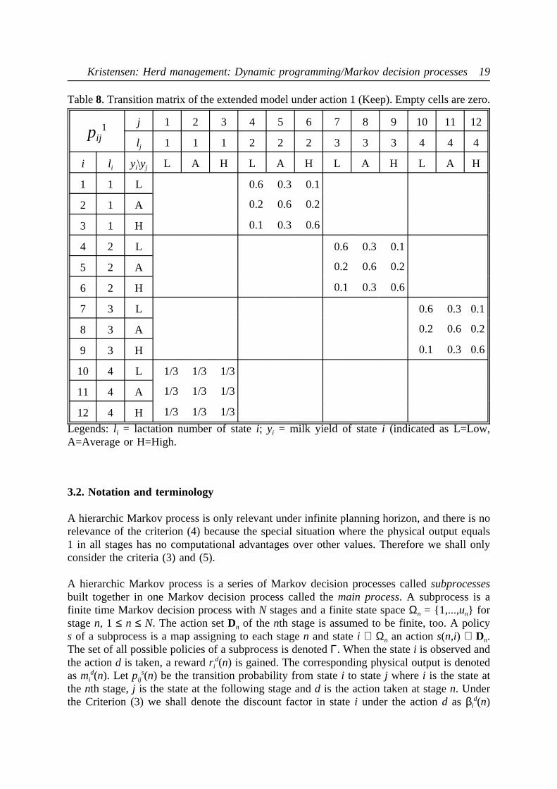
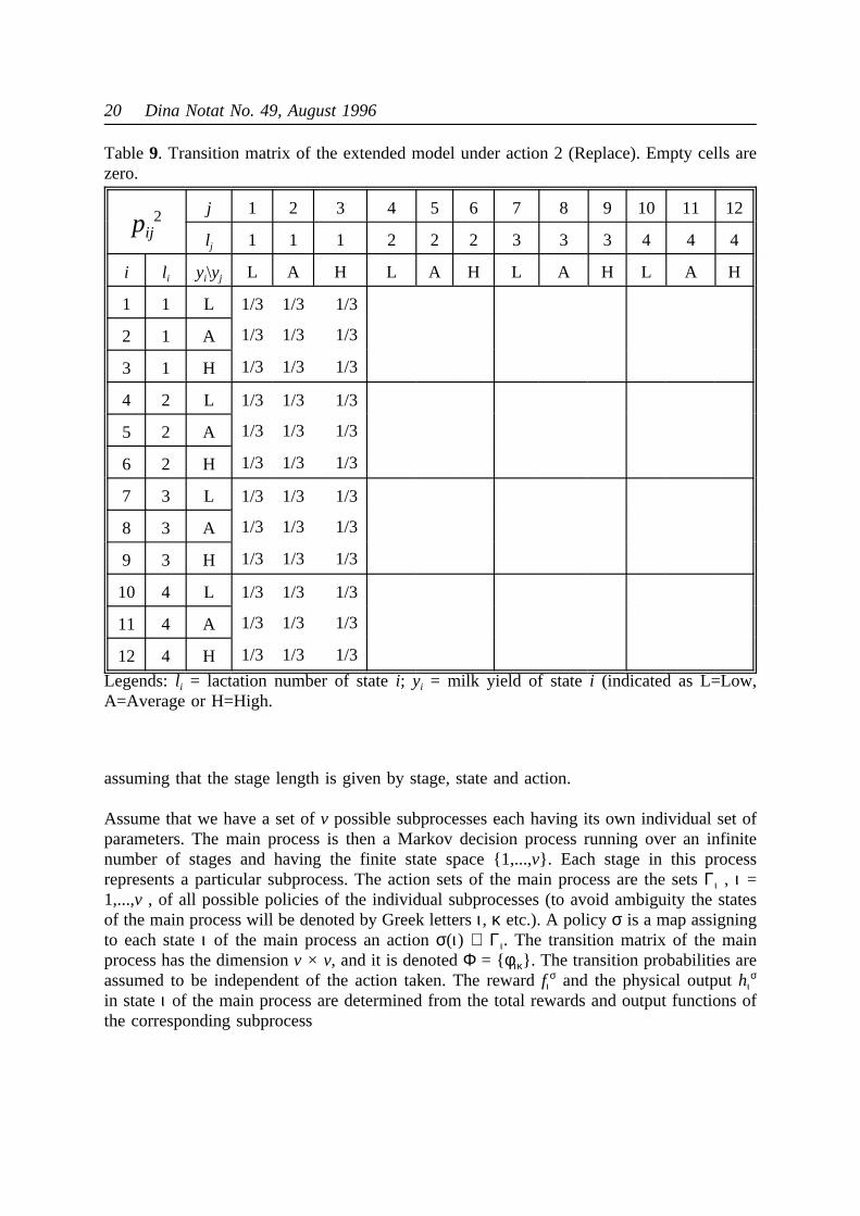
The transition matrices of the extended model are shown in Tables 8 and 9. It should beemphasizes that the state variable concerning milk yield should be interpreted relatively fora cow of the parity in question. As long as a cow is kept, it is assumed to change relativelevel of milk yield with the same probabilities as in the simple model, but when areplacement takes place, the new heifer is assumed to be low, average or high yielding withequal probabilities.
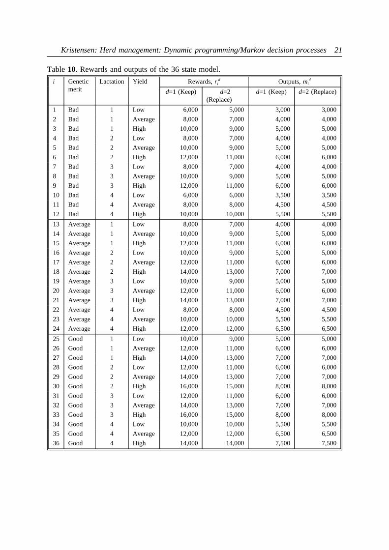
Inspection of the new matrices clearly illustrate that this very modest extension of the modelcauses a rather dramatic increase of the dimensions. Now, suppose that we in addition tolactation and milk yield also want to take the genetic merit into account. We shall assume thatthe genetic merit of the cow is either "Bad", "Average" or "Good". When a cow is replacedwe assume that the probability of the new heifer to be either genetically "Bad", "Average"or "Good" is 1/3 each. The total size of the state space then becomes 3 × 4 × 3 = 36. Themilk yields mi
d and rewardsrid appear from Table 10. The transition matrices of this 36-state
model are now very large. They are shown in the appendix as Tables 9, A.a - B.c for actions"Keep" and "Replace", respectively.
This stepwise extension of the model clearly illustrates that each time a new state variable atn levels is added to the model, the size of the state space is increased with a factor ofn.When, in a real model, several traits are represented by state variables at a realistic number
18 Dina Notat No. 49, August 1996
of levels, the size of the state space very soon reaches prohibitive dimensions (millions of
Table7. Rewards (annual net returns) and outputs (annual milk yield) of extended model.
i Lactation YieldRewards,ri
d Outputs,midOutputs,mid
d=1 (Keep) d=2 (Replace) d=1 (Keep) d=2 (Replace)
1 1 Low 8,000 7,000 4,000 4,000
2 1 Ave. 10,000 9,000 5,000 5,000
3 1 High 12,000 11,000 6,000 6,000
4 2 Low 10,000 9,000 5,000 5,000
5 2 Ave. 12,000 11,000 6,000 6,000
6 2 High 14,000 13,000 7,000 7,000
7 3 Low 10,000 9,000 5,000 5,000
8 3 Ave. 12,000 11,000 6,000 6,000
9 3 High 14,000 13,000 7,000 7,000
10 4 Low 8,000 8,000 4,500 4,500
11 4 Ave. 10,000 10,000 5,500 5,500
12 4 High 12,000 12,000 6,500 6,500
states). As an example, consider the dairy cow replacement model presented by Houben etal. (1994). The traits considered, when a decision was made, were- The age of the cow (204 levels)- Milk yield in present lactation (15 levels)- Milk yield in previous lactation (15 levels)- Time interval between 2 successive calvings (8 levels)- Clinical mastitis - an infectious disease in the udder (2 levels - yes/no)- Accumulated number of mastitis cases in present lactation (4 levels)- Accumulated number of mastitis cases in previous lactation (4 levels)In principle the size of the state space is formed as the product of the number of levels of alltraits, i.e. 204 × 15 × ... × 4 = 11,750,400 states. In practise it is smaller because somecombinations are impossible and because the traits related to previous lactation are notconsidered during first lactation. Exclusion of such not feasible states resulted in a model with6,821,724 different states. The model described only considers traits that vary over time forthe same animal. If furthermore, we wish to include permanent traits of the present animal(like the genetic merit of the 36-state model) being considered for replacement, the state spacewould become even larger. In order to circumvent this curse of dimensionality, Kristensen(1988; 1991) introduced a new notion of a hierarchic Markov process, which is described inthe following sections.
Kristensen: Herd management: Dynamic programming/Markov decision processes 19
3.2. Notation and terminology
Table8. Transition matrix of the extended model under action 1 (Keep). Empty cells are zero.
pij1 j 1 2 3 4 5 6 7 8 9 10 11 12
lj 1 1 1 2 2 2 3 3 3 4 4 4
i li yi\yj L A H L A H L A H L A H
1 1 L 0.6 0.3 0.1
2 1 A 0.2 0.6 0.2
3 1 H 0.1 0.3 0.6
4 2 L 0.6 0.3 0.1
5 2 A 0.2 0.6 0.2
6 2 H 0.1 0.3 0.6
7 3 L 0.6 0.3 0.1
8 3 A 0.2 0.6 0.2
9 3 H 0.1 0.3 0.6
10 4 L 1/3 1/3 1/3
11 4 A 1/3 1/3 1/3
12 4 H 1/3 1/3 1/3
Legends:li = lactation number of statei; yi = milk yield of statei (indicated as L=Low,A=Average or H=High.
A hierarchic Markov process is only relevant under infinite planning horizon, and there is norelevance of the criterion (4) because the special situation where the physical output equals1 in all stages has no computational advantages over other values. Therefore we shall onlyconsider the criteria (3) and (5).
A hierarchic Markov process is a series of Markov decision processes calledsubprocessesbuilt together in one Markov decision process called themain process. A subprocess is afinite time Markov decision process withN stages and a finite state spaceΩn = 1,...,un forstagen, 1 ≤ n ≤ N. The action setDn of the nth stage is assumed to be finite, too. A policys of a subprocess is a map assigning to each stagen and statei ∈ Ω n an actions(n,i) ∈ Dn.The set of all possible policies of a subprocess is denotedΓ. When the statei is observed andthe actiond is taken, a rewardri
d(n) is gained. The corresponding physical output is denotedasmi
d(n). Let pijs(n) be the transition probability from statei to statej wherei is the state at
the nth stage,j is the state at the following stage andd is the action taken at stagen. Underthe Criterion (3) we shall denote the discount factor in statei under the actiond as βi
d(n)
20 Dina Notat No. 49, August 1996
assuming that the stage length is given by stage, state and action.
Table9. Transition matrix of the extended model under action 2 (Replace). Empty cells arezero.
pij2 j 1 2 3 4 5 6 7 8 9 10 11 12
lj 1 1 1 2 2 2 3 3 3 4 4 4
i li yi\yj L A H L A H L A H L A H
1 1 L 1/3 1/3 1/3
2 1 A 1/3 1/3 1/3
3 1 H 1/3 1/3 1/3
4 2 L 1/3 1/3 1/3
5 2 A 1/3 1/3 1/3
6 2 H 1/3 1/3 1/3
7 3 L 1/3 1/3 1/3
8 3 A 1/3 1/3 1/3
9 3 H 1/3 1/3 1/3
10 4 L 1/3 1/3 1/3
11 4 A 1/3 1/3 1/3
12 4 H 1/3 1/3 1/3
Legends:li = lactation number of statei; yi = milk yield of statei (indicated as L=Low,A=Average or H=High.
Assume that we have a set ofv possible subprocesses each having its own individual set ofparameters. The main process is then a Markov decision process running over an infinitenumber of stages and having the finite state space 1,...,v. Each stage in this processrepresents a particular subprocess. The action sets of the main process are the setsΓι , ι =1,...,v , of all possible policies of the individual subprocesses (to avoid ambiguity the statesof the main process will be denoted by Greek lettersι , κ etc.). A policyσ is a map assigningto each stateι of the main process an actionσ(ι ) ∈ Γ ι. The transition matrix of the mainprocess has the dimensionv × v, and it is denotedΦ = φικ. The transition probabilities areassumed to be independent of the action taken. The rewardfι
σ and the physical outputhισ
in stateι of the main process are determined from the total rewards and output functions ofthe corresponding subprocess
Kristensen: Herd management: Dynamic programming/Markov decision processes 21
Table10. Rewards and outputs of the 36 state model.
i Geneticmerit
Lactation Yield Rewards,rid Outputs,mi
d
d=1 (Keep) d=2(Replace)
d=1 (Keep) d=2 (Replace)
1 Bad 1 Low 6,000 5,000 3,000 3,000
2 Bad 1 Average 8,000 7,000 4,000 4,000
3 Bad 1 High 10,000 9,000 5,000 5,000
4 Bad 2 Low 8,000 7,000 4,000 4,000
5 Bad 2 Average 10,000 9,000 5,000 5,000
6 Bad 2 High 12,000 11,000 6,000 6,000
7 Bad 3 Low 8,000 7,000 4,000 4,000
8 Bad 3 Average 10,000 9,000 5,000 5,000
9 Bad 3 High 12,000 11,000 6,000 6,000
10 Bad 4 Low 6,000 6,000 3,500 3,500
11 Bad 4 Average 8,000 8,000 4,500 4,500
12 Bad 4 High 10,000 10,000 5,500 5,500
13 Average 1 Low 8,000 7,000 4,000 4,000
14 Average 1 Average 10,000 9,000 5,000 5,000
15 Average 1 High 12,000 11,000 6,000 6,000
16 Average 2 Low 10,000 9,000 5,000 5,000
17 Average 2 Average 12,000 11,000 6,000 6,000
18 Average 2 High 14,000 13,000 7,000 7,000
19 Average 3 Low 10,000 9,000 5,000 5,000
20 Average 3 Average 12,000 11,000 6,000 6,000
21 Average 3 High 14,000 13,000 7,000 7,000
22 Average 4 Low 8,000 8,000 4,500 4,500
23 Average 4 Average 10,000 10,000 5,500 5,500
24 Average 4 High 12,000 12,000 6,500 6,500
25 Good 1 Low 10,000 9,000 5,000 5,000
26 Good 1 Average 12,000 11,000 6,000 6,000
27 Good 1 High 14,000 13,000 7,000 7,000
28 Good 2 Low 12,000 11,000 6,000 6,000
29 Good 2 Average 14,000 13,000 7,000 7,000
30 Good 2 High 16,000 15,000 8,000 8,000
31 Good 3 Low 12,000 11,000 6,000 6,000
32 Good 3 Average 14,000 13,000 7,000 7,000
33 Good 3 High 16,000 15,000 8,000 8,000
34 Good 4 Low 10,000 10,000 5,500 5,500
35 Good 4 Average 12,000 12,000 6,500 6,500
36 Good 4 High 14,000 14,000 7,500 7,500
22 Dina Notat No. 49, August 1996
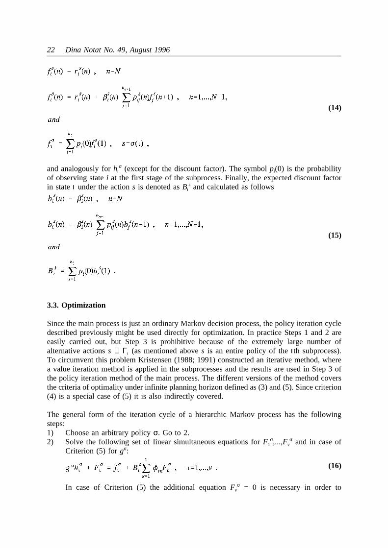
and analogously forhισ (except for the discount factor). The symbolpi(0) is the probability
(14)
of observing statei at the first stage of the subprocess. Finally, the expected discount factorin stateι under the actions is denoted asBι
s and calculated as follows
(15)
3.3. Optimization
Since the main process is just an ordinary Markov decision process, the policy iteration cycledescribed previously might be used directly for optimization. In practice Steps 1 and 2 areeasily carried out, but Step 3 is prohibitive because of the extremely large number ofalternative actionss ∈ Γ ι (as mentioned aboves is an entire policy of theι th subprocess).To circumvent this problem Kristensen (1988; 1991) constructed an iterative method, wherea value iteration method is applied in the subprocesses and the results are used in Step 3 ofthe policy iteration method of the main process. The different versions of the method coversthe criteria of optimality under infinite planning horizon defined as (3) and (5). Since criterion(4) is a special case of (5) it is also indirectly covered.
The general form of the iteration cycle of a hierarchic Markov process has the followingsteps:1) Choose an arbitrary policyσ. Go to 2.2) Solve the following set of linear simultaneous equations forF1
σ,...,Fvσ and in case of
Criterion (5) forgσ:
In case of Criterion (5) the additional equationFvσ = 0 is necessary in order to
(16)

Kristensen: Herd management: Dynamic programming/Markov decision processes 23
determine a unique solution. Go to 3.3) Define
under Criterion (3) andTι = 0 under Criterion (5). For each subprocessι , find by
(17)
means of the recurrence equations
a policy s’ of the subprocess. The actions’(n,i) is equal to thed’ that maximizes the
(18)
right hand side of the recurrence equation of statei at stagen. Put σ’(ι ) = s’ for ι =1,...,v. If σ’ = σ, then stop since an optimal policy is found. Otherwise, redefineσaccording to the new policy (i.e. putσ = σ’) and go back to 2.
When the iteration cycle is used under Criterion (3) all physical outputs (mid(n) and
accordingly alsohισ) are put equal to zero. The iteration cycle covering this situation was
developed by Kristensen (1988).
Under Criterion (4) all physical outputsmid(n) and all discount factorsβi
d(n) andBισ are put
equal to 1, but under Criterion (5) only the discount factors are put equal to 1. The iterationcycle covering these situations was described by Kristensen (1991).
3.4. Discussion and applications
The hierarchic Markov process is specially designed to fit the structure of animal decisionproblems where the successive stages of the subprocesses correspond to the age of the animalin question. By appropriate selection of state spaces in the subprocesses and the main processit is possible to find optimal solutions to even very large models. The idea is to let thenumber of states in the subprocesses (where a value iteration technique is applied) be verylarge and only include very few states in the main process (where the technique is directlybased on the policy iteration method). Thus we have got a method which is at the same timefast, exact and able to handle very large models.
Kristensen (1987) used the technique in a dairy cow replacement model which in a traditionalformulation as an ordinary Markov decision process would have contained approximately60000 states, and later (Kristensen, 1989) in a model with approximately 180 000 states. Inboth cases the number of states in the main process was only 5, reducing Step 2 to thesolution of only 5 simultaneous linear equations (versus 180 000 in a traditional formulation).Also Houben et al. (1994; 1995a,b) used the method in a dairy cow replacement model. Thereduction of the system of equations was in their case from 6,821,724 to just 1, because nopermanent traits were considered in the model. An interesting aspect of their model is thatfor the first time a disease is taken into account.
24 Dina Notat No. 49, August 1996
In sows, Huirne et al. (1992) seem to have applied a technique which in many aspects issimilar to a hierarchic Markov process, but they have not explained their method in all details.Also Jørgensen (1992) has applied a technique which is inspired of a hierarchic Markovprocess in a sow replacement model, and later (Jørgensen 1993), he used the hierarchicmethod in the determination of optimal delivery policies in slaughter pigs. Also Broekmans(1992) used the method in the determination of optimal delivery policies in slaugther pigstaking random variantion in prices into account. Verstegen et al. (1994) used the techniquein an experimental economics study investigating the utility value of management informationsystems. They used a formulation involving Bayesian updating of traits as described byKristensen (1993).
Naturally the hierarchic model just described may also be formulated as an ordinary Markovdecision process. In that case each combination of subprocess (main state), stage and stateshould be interpreted as a state. We shall denote a state in the transformed process as (ιni),and the parameters are
where the parameters mentioned on the right hand side of the equations are those belonging
(19)
to the ι th subprocess except forpi(0) which belongs to subprocessκ . This formulation ofcourse has the same optimal policies as the hierarchic formulation, so it is only computationaladvantages that make the hierarchic model relevant. A comparison to traditional methods maytherefore be relevant.
Since the policy iteration method involves the solution of a set ofu equations (whereu is thenumber of states) it is only relevant for small models. The value iteration method, however,has been used with even very large models and may handle problems of the same size as thehierarchic formulation, but the time spend on optimization is much lower under the hierarchicformulation. To recognize this, we shall compare the calculations involved.
Step 3 of the hierarchic optimization involves exactly the same number of operations as oneiteration of the value iteration method (Eq. (6)). The further needs of the hierarchic methodare the calculation of the rewards andeither the physical outputor the expected discountfactor of a stage in the main process according to Eqs. (14) and (15). Since the calculationsat each stage is only carried out for one action, the calculation of both main state parametersinvolves approximately the same number of operations as one iteration under the valueiteration method if the number of alternative actions is 2. If the number of actions is higher,
Kristensen: Herd management: Dynamic programming/Markov decision processes 25
the calculations relatively involves a lower number of operations than an iteration under thevalue iteration method. These considerations are based on the assumption that the valueiteration method is programmed in an efficient way, so that the sum of Eq. (6) is notcalculated as a sum of allu elements, but only as a sum of those elements wherepij
d is notzero according to Eq. (19). Otherwise the hierarchic technique will be even more superior.Finally the system of linear equations of Step 2 of the hierarchic cycle must be solved, butin large models with only a few states in the main process the time spent on this is negligible.
If we use the considerations above in a practical example, the advantages of the hierarchictechnique becomes obvious. As reported by Kristensen (1991) a model with 180,000 statecombinations was optimized by the hierarchic technique under 100 different price conditions.The number of iterations needed ranged from 3 to 6 corresponding to between 6 and 12iterations of the value iteration method. If the latter method was used instead, a planninghorizon of 20 years would be realistic (cf. van Arendonk 1985). Since each state in the modelequals 4 weeks, this horizon represents 260 iterations, which should be compared to theequivalence of from 6 to 12 when the hierarchic technique was applied.
3.5. The numerical example formulated and solved as a hierarchic Markov process
In order to illustrate the hierarchic technique, we shall formulate the numerical example (the36-state model) as a hierarchic Markov process. A PC program demonstrating hierarchicMarkov processes is available1. The following example is pre-defined and comes with theprogram.
The three classes of the genetic merit are defined as states in the main process of a hierarchicMarkov process. Thus the number of subprocesses is also 3 and each subprocess representsa dairy cow of a certain genetic merit. When a new heifer is purchased, we assume likebefore that the probability distribution over main states is uniform, so that the probability ofentering either one is 1/3. The maximum age of a cow was assumed to be 4 lactations, andthe states of the subprocess are defined from the relative level of milk yield. Further a dummystate of length, reward and output equal to 0 is included at each stage of the subprocesses.If the cow is replaced at the end of a stage, the process enters the dummy state withprobability 1 at the next stage, and for the rest of the duration of the subprocess it will stayin the dummy states. Stage numbers in the subprocesses directly correspond to lactationnumbers.
Thus, for all subprocesses the probability of staying at the same relative level of milk yield(state in the subprocess) is 0.6, and if the present state is "Average", the probability oftransition to either "Low" or "High" is 0.2 each. The probability of transition (if kept) from"Low" or "High" to "Average" is in both cases 0.3, and from "Low" to "High" and vice versathe probability is 0.1. The initial state probabilities of the subprocesses represent theprobability of a new heifer being either "Low", "Average" or "High" yielding. Thus, all initialstate probabilities are 1/3.
1 The program is available on World Wide Web as a ZIP-file. The file may bedownloaded from URL: http://www.prodstyr.husdyr.kvl.dk/Software/hierarchic.html
26 Dina Notat No. 49, August 1996
Like before, the physical outputs are interpreted as milk yields and the rewards are definedas the economic net returns. All parameters of the hierarchic model are shown in Tables 12and 11.
We shall determine an optimal solution under the following 3 criteria of optimality:
Table 11. Parameters of the hierarchic Markov process: Transition probabilities of mainprocess and initial state probabilities of subprocesses.
Transition probabilities, main process Initial state probabilities, subprocesses
Stateι
φικ pi(0)
κ=1 κ=2 κ=3 i=1 i=2 i=3 i=4
1 1/3 1/3 1/3 1/3 1/3 1/3 0
2 1/3 1/3 1/3 1/3 1/3 1/3 0
3 1/3 1/3 1/3 1/3 1/3 1/3 0
1) Maximization of total expected discounted rewards, i.e., the objective function (3). Inthis case the physical outputs of Table 2 are ignored, and a discount factorβi
d(n) =exp(-r), wherer is the interest rate, is applied (for states where the stage length is notzero).
2) Maximization of average rewards over time. In this situation we use the objectivefunction (5) letting the output represent stage length. No discounting is performed inthis case.
3) Maximization of average rewards over output defined as in Table 12. Thus the objectivefunction (5) is applied, and no discounting is performed.
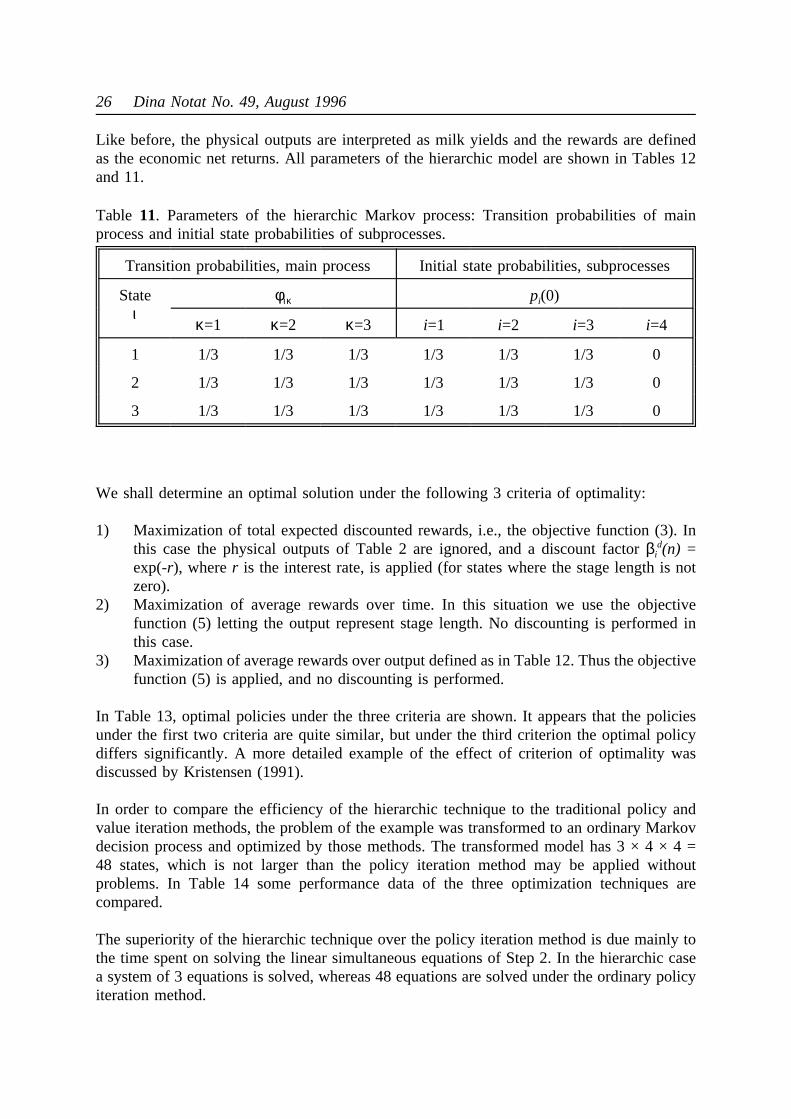
In Table 13, optimal policies under the three criteria are shown. It appears that the policiesunder the first two criteria are quite similar, but under the third criterion the optimal policydiffers significantly. A more detailed example of the effect of criterion of optimality wasdiscussed by Kristensen (1991).
In order to compare the efficiency of the hierarchic technique to the traditional policy andvalue iteration methods, the problem of the example was transformed to an ordinary Markovdecision process and optimized by those methods. The transformed model has 3 × 4 × 4 =48 states, which is not larger than the policy iteration method may be applied withoutproblems. In Table 14 some performance data of the three optimization techniques arecompared.
The superiority of the hierarchic technique over the policy iteration method is due mainly tothe time spent on solving the linear simultaneous equations of Step 2. In the hierarchic casea system of 3 equations is solved, whereas 48 equations are solved under the ordinary policyiteration method.

Kristensen: Herd management: Dynamic programming/Markov decision processes 27
In this numerical example the performance of the hierarchic technique is even more superior
Table12. Parameters of the hierarchic Markov process, subprocesses.
ι n ipij
1(n)ri
1(n) mi1(n)
pij2(n)
ri2(n) m2(n)
j=1 j=2 j=3 j=4 j=1 j=2 j=3 j=4
1 1 1 0.6 0.3 0.1 0.0 6,000 3,000 0.0 0.0 0.0 1.0 5,000 3,0001 1 2 0.2 0.6 0.2 0.0 8,000 4,000 0.0 0.0 0.0 1.0 7,0004,0001 1 3 0.1 0.3 0.6 0.0 10,000 5,000 0.0 0.0 0.0 1.0 9,0005,0001 1 4 0.0 0.0 0.0 1.0 0 0 0.0 0.0 0.0 1.0 0 01 2 1 0.6 0.3 0.1 0.0 8,000 4,000 0.0 0.0 0.0 1.0 7,0004,0001 2 2 0.2 0.6 0.2 0.0 10,000 5,000 0.0 0.0 0.0 1.0 9,0005,0001 2 3 0.1 0.3 0.6 0.0 12,000 6,000 0.0 0.0 0.0 1.0 11,0006,0001 2 4 0.0 0.0 0.0 1.0 0 0 0.0 0.0 0.0 1.0 0 01 3 1 0.6 0.3 0.1 0.0 8,000 4,000 0.0 0.0 0.0 1.0 7,0004,0001 3 2 0.2 0.6 0.2 0.0 10,000 5,000 0.0 0.0 0.0 1.0 9,0005,0001 3 3 0.1 0.3 0.6 0.0 12,000 6,000 0.0 0.0 0.0 1.0 11,0006,0001 3 4 0.0 0.0 0.0 1.0 0 0 0.0 0.0 0.0 1.0 0 01 4 1 - - - - 6,000 3,500 - - - - 6,000 3,5001 4 2 - - - - 8,000 4,500 - - - - 8,000 4,5001 4 3 - - - - 10,000 5,500 - - - - 10,000 5,5001 4 4 - - - - 0 0 - - - - 0 02 1 1 0.6 0.3 0.1 0.0 8,000 4,000 0.0 0.0 0.0 1,0 7,000 4,0002 1 2 0.2 0.6 0.2 0.0 10,000 5,000 0.0 0.0 0.0 1.0 9,0005,0002 1 3 0.1 0.3 0.6 0.0 12,000 6,000 0.0 0.0 0.0 1.0 11,0006,0002 1 4 0.0 0.0 0.0 1.0 0 0 0.0 0.0 0.0 1.0 0 02 2 1 0.6 0.3 0.1 0.0 10,000 5,000 0.0 0.0 0.0 1.0 9,0005,0002 2 2 0.2 0.6 0.2 0.0 12,000 6,000 0.0 0.0 0.0 1.0 11,0006,0002 2 3 0.1 0.3 0.6 0.0 14,000 7,000 0.0 0.0 0.0 1.0 13,0007,0002 2 4 0.0 0.0 0.0 1.0 0 0 0.0 0.0 0.0 1.0 0 02 3 1 0.6 0.3 0.1 0.0 10,000 5,000 0.0 0.0 0.0 1.0 9,0005,0002 3 2 0.2 0.6 0.2 0.0 12,000 6,000 0.0 0.0 0.0 1.0 11,0006,0002 3 3 0.1 0.3 0.6 0.0 14,000 7,000 0.0 0.0 0.0 1.0 13,0007,0002 3 4 0.0 0.0 0.0 1.0 0 0 0.0 0.0 0.0 1.0 0 02 4 1 - - - - 8,000 4,500 - - - - 8,000 4,5002 4 2 - - - - 10,000 5,500 - - - - 10,000 5,5002 4 3 - - - - 12,000 6,500 - - - - 12,000 6,5002 4 4 - - - - 0 0 - - - - 0 03 1 1 0.6 0.3 0.1 0.0 10,000 5,000 0.0 0.0 0.0 1.0 9,000 5,0003 1 2 0.2 0.6 0.2 0.0 12,000 6,000 0.0 0.0 0.0 1.0 11,0006,0003 1 3 0.1 0.3 0.6 0.0 14,000 7,000 0.0 0.0 0.0 1.0 13,0007,0003 1 4 0.0 0.0 0.0 1.0 0 0 0.0 0.0 0.0 1.0 0 03 2 1 0.6 0.3 0.1 0.0 12,000 6,000 0.0 0.0 0.0 1.0 11,0006,0003 2 2 0.2 0.6 0.2 0.0 14,000 7,000 0.0 0.0 0.0 1.0 13,0007,0003 2 3 0.1 0.3 0.6 0.0 16,000 8,000 0.0 0.0 0.0 1.0 15,0008,0003 2 4 0.0 0.0 0.0 1.0 0 0 0.0 0.0 0.0 1.0 0 03 3 1 0.6 0.3 0.1 0.0 12,000 6,000 0.0 0.0 0.0 1.0 11,0006,0003 3 2 0.2 0.6 0.2 0.0 14,000 7,000 0.0 0.0 0.0 1.0 13,0007,0003 3 3 0.1 0.3 0.6 0.0 16,000 8,000 0.0 0.0 0.0 1.0 15,0008,0003 3 4 0.0 0.0 0.0 1.0 0 0 0.0 0.0 0.0 1.0 0 03 4 1 - - - - 10,000 5,500 - - - - 10,000 5,5003 4 2 - - - - 12,000 6,500 - - - - 12,000 6,5003 4 3 - - - - 14,000 7,500 - - - - 14,000 7,5003 4 4 - - - - 0 0 - - - - 0 0
Legends:ι = Subprocess (Main State),n = Stage number,i = State at Stagen, j = State at Stagen+1.

28 Dina Notat No. 49, August 1996
to the value iteration method than expected from the theoretical considerations of Section 3.4.
Table13. Optimal policies under the three criteria (c1, c2, c3) defined in the text (actions: 1= "Keep", 2 = "Replace").
Subprocess StageState 1 State 2 State 3
c1 c2 c3 c1 c2 c3 c1 c2 c3
1 1 2 2 1 2 2 1 2 1 1
1 2 2 2 1 2 2 1 2 1 1
1 3 2 2 1 2 2 1 2 2 1
2 1 1 1 1 1 1 1 1 1 1
2 2 2 1 1 1 1 1 1 1 1
2 3 2 2 1 2 1 1 1 1 1
3 1 1 1 1 1 1 1 1 1 1
3 2 1 1 1 1 1 1 1 1 1
3 3 1 1 1 1 1 1 1 1 1
Table 14. The performance of the hierarchic technique compared to the policy and valueiteration methods under the three criteria (c1, c2, c3) defined in the text.
Hierachic model Policy iteration Value iteration
c1 c2 c3 c1 c2 c3 c1 c2 c3
Number of iterations 4 3 2 4 4 2 100 100 100
Computer time, relatively 1 0.86 0.43 268 267 139 48 46 11
In the present case an iteration of the hierarchic model is performed even faster than one ofthe value iteration method applied to the same (transformed) model. The reason is that thevalue iteration algorithm has not been programmed in the most efficient way as defined inSection 3.4. On the contrary, the sum of Eq. 3 has been calculated over all 48 states of thetransformed model. Since only 4 transition probabilities from each state are positive, the sumcould be calculated only over these 4 states.
4. Uniformity: Bayesian updating
As discussed earlier, it is obvious that the traits of an animal varies no matter whether we areconsidering the milk yield of a dairy cow, the litter size of a sow or almost any other trait.On the other hand, it isnot obvious to what extent theobserved trait Yn at stagen is, for
Kristensen: Herd management: Dynamic programming/Markov decision processes 29
instant, the result of a permanent property of the animalX1, a permanent damage caused bya previous diseaseX2 or a temporary random fluctuationen. Most often the observed valueis the result of several permanent and random effects. WithYn, X1, X2 anden defined as abovethe relation might for instance be
wherem is the expected value for an arbitrarily selected animal under the circumstances in
(20)
question, anda = -1 if the animal has been suffering from the disease, anda = 0 otherwise.In this exampleX1 only variesamong animals, whereasen also variesover time for the sameanimal. The effect of the damage caused by the diseaseX2 is in this example assumed to beconstant over time when it has been "switched on". The value ofX2 is a property of theindividual disease case (the "severity" of the case).
In a replacement decision it is of course important to know whether the observed value ismainly a result of a permanent effect or it is just the result of a temporary fluctuation. Theproblem, however, is that only the resulting valueYn is observed, whereas the values ofX1,X2 and en are unknown. On the other hand, as observations ofY1, Y2,... are done we arelearning something about the value of the permanent effects. Furthermore, we have got aprior distribution ofX1 andX2, and each time an observation is done, we are able to calculatethe posterior distribution of X1 and X2 by means of the Kalman-filter theory (described forinstance by Harrison and Stevens, 1976) if we assume all effects to be normally distributed.
A model as described by Eq. (20) fits very well into the structure of a hierarchic Markovprocess. Thus we may regardYn as a state variable in a subprocess, and the permanent effectsX1 andX2 as state variables of the main process. We then face a hierarchic Markov processwith unobservable main state. Kristensen (1993) discusses this notion in details, and it isshown that under the assumption of normally distributed effects, we only have to keep thepresent expected values ofX1 andX2, the currently observed value ofYn and (in this example)the number of stages since the animal was suffering from the disease (if it has been sufferingfrom the disease at all). The expectations ofX1 andX2 are sufficient to determine the currentposterior distribution of the variables, because the variance is known in advance. Even thoughthe posterior variance decreases as observations are done, the decrease doesnot depend onthe values of Y1, Y2,... but only on the number of observations done.
In the study of Kristensen (1993), a more general case involving several traits each beinginfluenced by several unobservable effects is sketched, and a numerical example involvingonly a single trait is given. An example concerning replacement of sows has been given byJørgensen (1992). It was demonstrated in both studies that the Bayesian approach in somecases may result in state space reduction without loss of information. In multi-trait updatingmodels a Kalman filter technique may be relevant as described by Kristensen (1994).
5. Herd restraints: Parameter iteration
One of the major difficulties identified in the introduction washerd restraints. All thereplacement models mentioned in the previous sections have been single-component models,i.e., only one animal is considered at the same time, assuming an unlimited supply of allresources (heifers or gilts for replacement, feed, labour etc) and no production quota. In a
30 Dina Notat No. 49, August 1996
multi-component model all animals of a herd are simultaneously considered for replacement.If all animals (components) compete for the same limited resource or quota, the replacementdecision concerning an animal does not only depend on the state of that particular animal, butalso on the states of the other animals (components) of the herd.
If the only (or at least themost limiting) herd restraint is a limited housing capacity, thenumber of animals in production is the scarce resource, and accordingly the relevant criterionof optimality is the maximization of net revenues per animal as it is expressed in the criteria(1), (2), (3) and (4). Thus the optimal replacement policy of the single component model isoptimal for the multi-component model too.
If the only (or most limiting) herd restraint is a milk quota, the situation is much morecomplicated. Since the most limiting restriction is a fixed amount of milk to produce, therelevant criterion of optimality is now the maximization of average net revenues per kg milkyield as expressed in criterion (5), because a policy that maximizes net revenues per kg milkwill also maximize total net revenues from the herd which was assumed to be the objectiveof the farmer.
By following a policy which is optimal according to criterion (5) we assure at any time thatthe cows which produce milk in the cheapest way are kept. Thus the problem of selectingwhich cows to keep in the long run (and the mutual ranking of cows) is solved, but theproblem of determining the optimal number of cows in production at any time isnot solved.If for instance, it is recognized 2 months before the end of the quota year that the quota isexpected to be exceeded by 10 percent, we have to choose whether to reduce the herd sizeor to keep the cows and pay the penalty. The problem is that both decisions will influencethe possibilities of meeting the quota of the next year in an optimal way. To solve this shortrun quota adjustment problem we need a true multi-component model.
An other example of a herd restraint is a limited supply of heifers. If the dairy farmer onlyuses home-grown heifers for replacement, the actions concerning individual cows becomeinter-dependent, and again a multi-component model is needed in order to solve thereplacement problem. Ben-Ari and Gal (1986) and later Kristensen (1992) demonstrated thatthe replacement problem in a dairy herd with cows and a limited supply of home grownheifers may be formulated as a Markov decision process involving millions of states. Thismulti-component model is based on a usual single-component Markov decision processrepresenting one cow and its future successors. Even though the hierarchic technique hasmade the solution of even very large models possible, such a model is far too large foroptimization in practice. Therefore, the need for an approximate method emerged, and amethod calledparameter iteration was introduced by Ben-Ari and Gal (1986).
The basic idea of the method is to approximate either the present value functionfi(n)(objective function (3)) or the relative valuesfi
s (objective functions (4) and (5)) by a functionG involving a set of parametersa1,...,am to be determined in such a way thatG(i,a1,...,am) ≈fi(n) or G(i,a1,...,am) ≈ fi
s .
In the implementation of Ben-Ari and Gal (1986) the parameters were determined by aniterative technique involving the solution of sets of simultaneous linear equations generated
Kristensen: Herd management: Dynamic programming/Markov decision processes 31
by simulation.
In a later implementation Kristensen (1992) determined the parameters by ordinary leastsquares regression on a simulated data set. The basic idea of the implementation is to takeadvantage from the fact that we are able to determine an optimal solution to the underlying(unrestricted) single-component model. If no herd restraint was present, the present value ofthe multi-component model would equal the sum of the present values of the individualanimals determined from the underlying single-component model. Then it is argued in whatway the restraint will logically reduce the (multi-component) present value, and a functionalexpression having the desired properties is chosen. The parameters of the function areestimated from a simulated data set, and the optimal action for a given (multi-component)state is determined as the one that maximizes the corrected present value. (A state in themulti-component model is defined from the states of the individual animals in the single-component model, and an action defines the replacement decision of each individual animal).
Ben-Ari and Gal (1986) compared the economic consequences of the resulting optimal multi-component policy to a policy defined by dairy farmers, and they showed that the policy fromthe parameter iteration method was better. Kristensen (1992) compared the optimal multi-component policies to policies from usual single-component models in extensive stochasticsimulations and showed that the multi-component policies were superior in situations withshortage of heifers.
The parameter iteration method has been applied under a limited supply of heifers. It seemsto be realistic to expect, that the method and the basic principles of Kristensen (1992) maybe used under other kinds of herd restraints as for instance the short time adjustment to a milkquota as mentioned above.
6. General discussion
In the introduction, the main difficulties concerning animal production models were identifiedas variability in traits, cyclic production, uniformity (the traits are difficult to define andmeasure) andherd restraints. We are now able to conclude that the difficulties of variabilityand the cyclic production are directly solved by the application of Markov decisionprogramming, but when the variability of several traits are included we face a problem ofdimensionality. The formulation of the notion of ahierarchic Markov process contributed tothe solution of the dimensionality problem, but did not solve it. The upper limit of numberof states to be included has been raised considerably, but not eliminated.
This is for instance clearly illustrated when we formulatemulti-component herd models inorder to deal with herd restraints. In that case we still have to use approximate methods todetermine an "optimal" replacement policy. On the other hand it has been demonstrated byKristensen (1992) that theparameter iteration method applied to a multi-component herdmodel (even though it is only approximate) is able to improve the total net revenue comparedto the application of a usual single-component (animal) model in a situation with shortage ofheifers. The parameter iteration method is an important contribution to the problem ofdetermining optimal replacement policies under herd restraints.
32 Dina Notat No. 49, August 1996
In other situations with a limiting herd restraint it may be relevant to use an alternativecriterion of optimality maximizing average net revenue per unit of the limiting factor. Thismethod has been successfully applied in a situation with milk production under a limitingquota.
Recent results have also contributed to the solution of the uniformity problem. The Bayesianupdating technique described in Section 4 seems to be a promising approach, but it has notyet been tested on real data. It might be a solution to the problem of including animal healthas a trait to be considered. As concerns other traits such as litter size or milk yield theBayesian approach may in some cases result in a reduction of the state space without loss ofinformation (Jørgensen, 1992; Kristensen, 1993). Thus it contributes indirectly to the solutionof the dimensionality problem.
New developments in the area of Markov decision programming for herd management supportincludes the notion of multi-level hierarchic models, where actions are defined at differentlevels with different time horizons. Thus the method is able to optimize decisions withdifferent time horizons simultaneously as described by Kristensen & Jørgensen (1996a,b).
References
Ben-Ari, Y. and Gal, S. 1986. Optimal replacement policy for multicomponent systems: Anapplication to a dairy herd.European Journal of Operational Research 23, 213-221.
Ben-Ari, Y., Amir, I. and Sharar, S. 1983. Operational replacement decision model for dairyherds.Journal of Dairy Science 66, 1747-1759.
Bellman, R. E. (1957).Dynamic Programming. Princeton: Princeton University Press.Bellman, R. E. (1961).Adaptive control processes: a guided tour. Princeton: Princeton
University Press.Bellman, R. E. and Dreyfus, S. E. 1962.Applied dynamic programming. Princeton: Princeton
University Press.Bellman, R. E. and Kalaba, R. 1965.Dynamic programming and modern control theory. New
York: Academic Press.Broekmans, J.E. 1992. Influence of price fluctuations on delivery strategies for slaughter pigs.
Dina Notat No. 7.DeLorenzo, M.A., T.H. Spreen, G.R. Bryan, D.K. Beede and J.A.M. van Arendonk. 1992.
Optimizing model: insemination, replacement, seasonal variation, and cash flow.Journalof Dairy Science 75, 885-896.
Giaever, H. B. 1966.Optimal dairy cow replacement policies. Ph. D. dissertation. Ann Ar-bor, Michigan: University Microfilms.
Hadley, G. 1964.Nonlinear and dynamic programming. Reading, Massachusetts: Addison-Wesley.
Harrison, P. J. and Stevens, C. F. 1976. Bayesian forecasting.Journal of the Royal StatisticalSociety B 38, 205-247.
Houben, E.H.P., R.B.M. Huirne, A.A. Dijkhuizen and A.R. Kristensen. 1994. Optimalreplacement of mastitis cows determined by a hierarchic Markov process.Journal ofdairy Science 77, 2975-2993.
Houben, E.H.P., A.A. Dijkhuizen, R.B.M. Huirne and A. Brand. 1995a. The economic valueof information on mastitis in making dairy cow replacement decisions.Journal of Dairy
Kristensen: Herd management: Dynamic programming/Markov decision processes 33
Science. In press.Houben, E.H.P., A.A. Dijkhuizen, R.B.M. Huirne and J.A. Renkema. 1995b. The effect of
milk quotas on optimal dairy cow insemination and replacement decisions. Submittedto Livestock Production Science.
Howard, R. A. 1960.Dynamic programming and Markov processes. Cambridge, Massa-chusetts: The M.I.T. Press.
Howard, R. A. 1971.Dynamic probabilistic systems. Volume II: Semi-Markov and decisionprocesses. New York: John Wiley & Sons, Inc.
Huirne, R. B. M., Hendriks, Th. H. B., Dijkhuizen, A. A. and Giesen, G. W. J. 1988. Theeconomic optimization of sow replacement decisions by stochastic dynamic program-ming. Journal of Agricultural Economics 39, 426-438.
Huirne, R. B. M., van Beek, P., Hendriks, Th. H. B. and Dijkhuizen, A. A. 1992. Anapplication of stochastic dynamic programming to support sow replacement decisions.European Journal of Operational Research. In press.
Jenkins, K. B. and Halter, A. N. 1963. A multistage stochastic replacement decision model:Application to replacement of dairy cows.Technical Bulletin 67, Agr. Exp. Sta., OregonState University.
Jewell, W. 1963. Markov renewal programming I and II.Operations Research 11, 938-971.Johnston, J. 1965. Dynamic programming and the theory of the firm.Journal of Agricultural
Economics 16, 532-543.Jørgensen, E. 1992. Sow replacement: Reduction of state space in Dynamic Programming
model and evaluation of benefit from using the model. Unpublished manuscript.Jørgensen, E. 1993. The influence of weighing precision on delivery decisions in slaughter
pig production.Acta Agriculturæ Scandinavica. Section A, Animal Science 43, 181-189.Kennedy, J. O. S. 1981. Applications of dynamic programming to agriculture, forestry and
fisheries: Review and prognosis.Review of Marketing and Agricultural Economics 49,141-173.
Kennedy, J. O. S. 1986.Dynamic programming. Applications to agriculture and naturalresources. London and New York: Elsevier applied science publishers.
Killen, L. and Kearney, B. 1978. Optimal dairy cow replacement policy.Irish Journal ofAgricultural Economics and Rural Sociology 7, 33-40.
Kristensen, A. R. 1987. Optimal replacement and ranking of dairy cows determined by ahierarchic Markov process.Livestock Production Science 16, 131-144.
Kristensen, A. R. 1988. Hierarchic Markov processes and their applications in replacementmodels.European Journal of Operational Research 35, 207-215.
Kristensen, A. R. 1989. Optimal replacement and ranking of dairy cows under milk quotas.Acta Agriculturæ Scandinavica 39, 311-318.
Kristensen, A. R. 1991. Maximization of net revenue per unit of physical output in Markovdecision processes.European Review of Agricultural Economics 18, 231-244.
Kristensen, A. R. 1992. Optimal replacement in the dairy herd: A multi-component system.Agricultural Systems 39, 1-24.
Kristensen, A. R. 1993. Bayesian updating in hierarchic Markov processes applied to theanimal replacement problem.European Review of Agricultural Economics 20. In press.
Kristensen, A.R. 1994. Dynamic programming as a framework for decision support in animalproduction.Dina Notat No. 27. URL: ftp://ftp.dina.kvl.dk/pub/Dina-reports/notat27.ps
Kristensen, A.R. & Jørgensen, E. 1995. Applicational perspectives of recent developments indynamic programming methods for herd management support.Dina Notat No. 33. URL:
34 Dina Notat No. 49, August 1996
ftp://ftp.dina.kvl.dk/pub/Dina-reports/notat33.psKristensen, A.R. & Jørgensen, E. 1996a. Multi-level hierarchic Markov processes as a
framework for herd management support.Dina Research Report No. 41. URL:ftp://ftp.dina.kvl.dk/pub/Dina-reports/resear41.ps
Kristensen, A.R. & E. Jørgensen. 1996b. Simultaneous optimization of management decisionsat the operational and tactical level in animal production. In: Risk ManagementStrategies in Agriculture: State of the Art and Future Perspectives. EUNITA-Seminar,January 7-10, 1996, Wageningen, The Netherlands.
Kristensen, A. R. and Thysen, I. 1991. Economic value of culling information in the presenceand absence of a milk quota.Acta Agriculturæ Scandinavica 41, 129-135.
Kristensen, A. R. and Østergaard, V. 1982. Optimalt udskiftningstidspunkt for malkekoenfastlagt ved en stokastisk model. (In Danish with English summary).Beretning fraStatens Husdyrbrugsforsøg 533.
McArthur, A. T. G. 1973. Application of dynamic programming to the culling decision indairy cattle.Proceedings of the New Zealand Society of Animal Production 33, 141-147.
Reenberg, H. 1979. Udskiftning af malkekøer. En stokastisk udskiftningsmodel. (In Danishwith English summary).Memorandum 6, Jordbrugsøkonomisk Institut.
Ross, S. M. 1970.Applied probability models with optimization applications. San Francisco,California: Holden-Day.
Smith, B. J. 1971. The dairy cow replacement problem. An application of dynamic program-ming. Bulletin 745. Florida Agricultural Experiment Station. Gainesville, Florida.
Stewart, H. M., Burnside, E. B. and Pfeiffer, W. C. 1978. Optimal culling strategies for dairycows of different breeds.Journal of Dairy Science 61, 1605-1615.
Stewart, H. M., Burnside, E. B., Wilton, J. W. and Pfeiffer, W. C. 1977. A dynamicprogramming approach to culling decisions in commercial dairy herds.Journal of DairyScience 60, 602-617.
van Arendonk, J. A. M. 1984. Studies on the replacement policies in dairy cattle. I.Evaluation of techniques to determine the optimum time for replacement and to rankcows on future profitability.Zeitschrift für Tierzüchtung und Züchtungsbiologi 101, 330-340.
van Arendonk, J. A. M. 1985. Studies on the replacement policies in dairy cattle. II. Optimumpolicy and influence of changes in production and prices.Livestock Production Science13, 101-121.
van Arendonk, J. A. M. 1986. Studies on the replacement policies in dairy cattle. IV.Influence of seasonal variation in performance and prices.Livestock Production Science14, 15-28.
van Arendonk, J. A. M. 1988. Management guides for insemination and replacementdecisions.Journal of Dairy Science 71, 1050-1057.
van Arendonk, J. A. M. and Dijkhuizen, A. A. 1985. Studies on the replacement policies indairy cattle. III. Influence of variation in reproduction and production.LivestockProduction Science 13, 333-349.
van der Wal, J. and Wessels, J. 1985. Markov decision processes.Statistica Neerlandica 39,219-233.
Verstegen, J.A.A.M., J. Sonnemans, E.H.J. Braakman, R.B.M. Huirne and A.A. Dijkhuizen.1994. Survey studies and experimental economic methods to investigate farmersdecision making and profitability of management information systems.Proceedings ofthe 38. EAAE Seminar on Farmers Decision Making - A descriptive approach.

Kristensen: Herd management: Dynamic programming/Markov decision processes 35
Copenhagen, Denmark, October 3-5, 1994.White, C. C. III and White, D. J. 1989. Markov decision processes.European Journal of
Operational Research 39, 1-16.
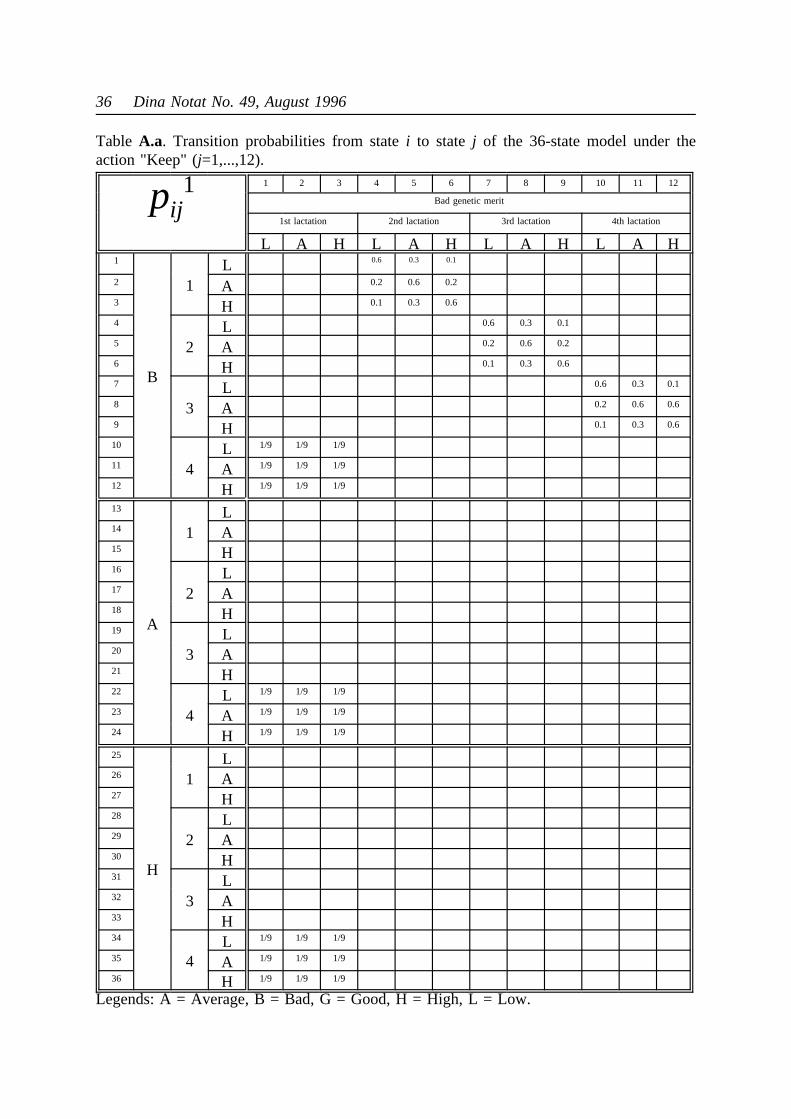
36 Dina Notat No. 49, August 1996
Table A.a. Transition probabilities from statei to statej of the 36-state model under theaction "Keep" (j=1,...,12).
pij1 1 2 3 4 5 6 7 8 9 10 11 12
Bad genetic merit
1st lactation 2nd lactation 3rd lactation 4th lactation
L A H L A H L A H L A H1
B
1L 0.6 0.3 0.1
2 A 0.2 0.6 0.2
3 H 0.1 0.3 0.6
4
2L 0.6 0.3 0.1
5 A 0.2 0.6 0.2
6 H 0.1 0.3 0.6
7
3L 0.6 0.3 0.1
8 A 0.2 0.6 0.6
9 H 0.1 0.3 0.6
10
4L 1/9 1/9 1/9
11 A 1/9 1/9 1/9
12 H 1/9 1/9 1/9
13
A
1L
14 A15 H16
2L
17 A18 H19
3L
20 A21 H22
4L 1/9 1/9 1/9
23 A 1/9 1/9 1/9
24 H 1/9 1/9 1/9
25
H
1L
26 A27 H28
2L
29 A30 H31
3L
32 A33 H34
4L 1/9 1/9 1/9
35 A 1/9 1/9 1/9
36 H 1/9 1/9 1/9
Legends: A = Average, B = Bad, G = Good, H = High, L = Low.
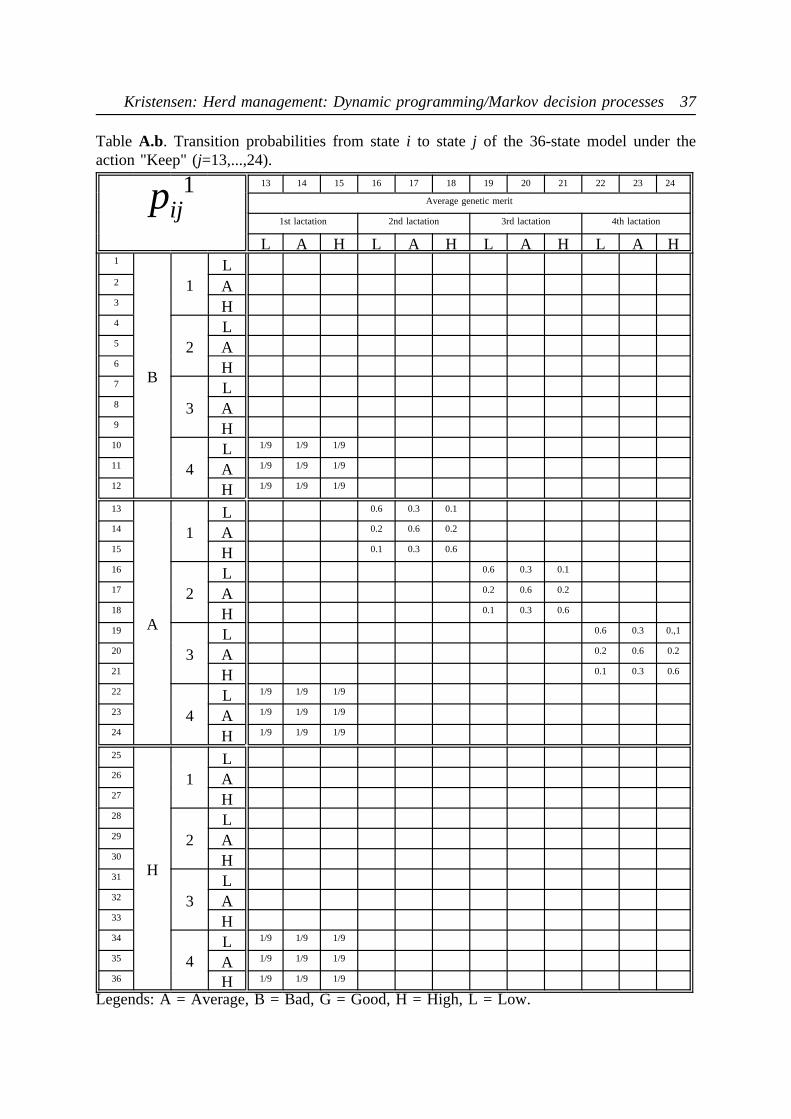
Kristensen: Herd management: Dynamic programming/Markov decision processes 37
Table A.b. Transition probabilities from statei to statej of the 36-state model under theaction "Keep" (j=13,...,24).
pij1 13 14 15 16 17 18 19 20 21 22 23 24
Average genetic merit
1st lactation 2nd lactation 3rd lactation 4th lactation
L A H L A H L A H L A H1
B
1L
2 A3 H4
2L
5 A6 H7
3L
8 A9 H10
4L 1/9 1/9 1/9
11 A 1/9 1/9 1/9
12 H 1/9 1/9 1/9
13
A
1L 0.6 0.3 0.1
14 A 0.2 0.6 0.2
15 H 0.1 0.3 0.6
16
2L 0.6 0.3 0.1
17 A 0.2 0.6 0.2
18 H 0.1 0.3 0.6
19
3L 0.6 0.3 0.,1
20 A 0.2 0.6 0.2
21 H 0.1 0.3 0.6
22
4L 1/9 1/9 1/9
23 A 1/9 1/9 1/9
24 H 1/9 1/9 1/9
25
H
1L
26 A27 H28
2L
29 A30 H31
3L
32 A33 H34
4L 1/9 1/9 1/9
35 A 1/9 1/9 1/9
36 H 1/9 1/9 1/9
Legends: A = Average, B = Bad, G = Good, H = High, L = Low.
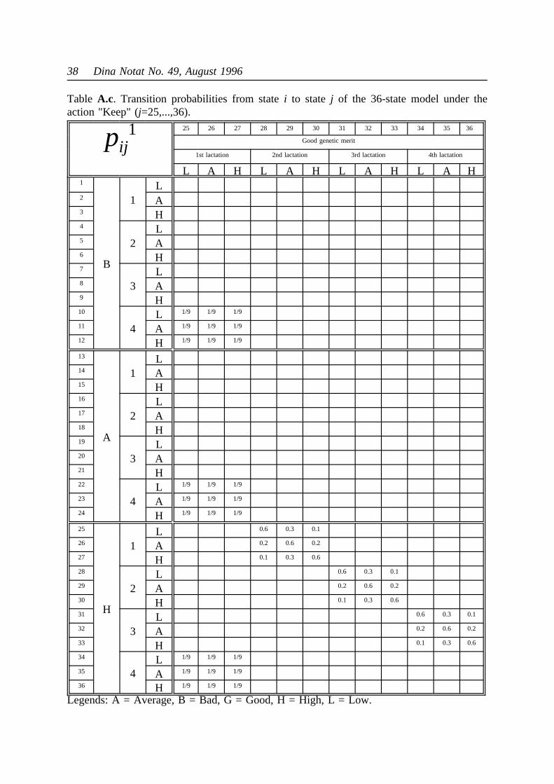
38 Dina Notat No. 49, August 1996
Table A.c. Transition probabilities from statei to statej of the 36-state model under theaction "Keep" (j=25,...,36).
pij1 25 26 27 28 29 30 31 32 33 34 35 36
Good genetic merit
1st lactation 2nd lactation 3rd lactation 4th lactation
L A H L A H L A H L A H1
B
1L
2 A3 H4
2L
5 A6 H7
3L
8 A9 H10
4L 1/9 1/9 1/9
11 A 1/9 1/9 1/9
12 H 1/9 1/9 1/9
13
A
1L
14 A15 H16
2L
17 A18 H19
3L
20 A21 H22
4L 1/9 1/9 1/9
23 A 1/9 1/9 1/9
24 H 1/9 1/9 1/9
25
H
1L 0.6 0.3 0.1
26 A 0.2 0.6 0.2
27 H 0.1 0.3 0.6
28
2L 0.6 0.3 0.1
29 A 0.2 0.6 0.2
30 H 0.1 0.3 0.6
31
3L 0.6 0.3 0.1
32 A 0.2 0.6 0.2
33 H 0.1 0.3 0.6
34
4L 1/9 1/9 1/9
35 A 1/9 1/9 1/9
36 H 1/9 1/9 1/9
Legends: A = Average, B = Bad, G = Good, H = High, L = Low.
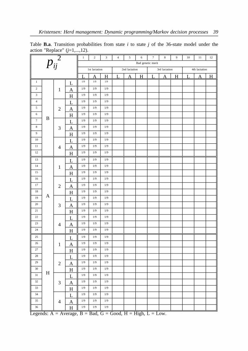
Kristensen: Herd management: Dynamic programming/Markov decision processes 39
Table B.a. Transition probabilities from statei to statej of the 36-state model under theaction "Replace" (j=1,...,12).
pij2 1 2 3 4 5 6 7 8 9 10 11 12
Bad genetic merit
1st lactation 2nd lactation 3rd lactation 4th lactation
L A H L A H L A H L A H1
B
1L 1/9 1/9 1/9
2 A 1/9 1/9 1/9
3 H 1/9 1/9 1/9
4
2L 1/9 1/9 1/9
5 A 1/9 1/9 1/9
6 H 1/9 1/9 1/9
7
3L 1/9 1/9 1/9
8 A 1/9 1/9 1/9
9 H 1/9 1/9 1/9
10
4L 1/9 1/9 1/9
11 A 1/9 1/9 1/9
12 H 1/9 1/9 1/9
13
A
1L 1/9 1/9 1/9
14 A 1/9 1/9 1/9
15 H 1/9 1/9 1/9
16
2L 1/9 1/9 1/9
17 A 1/9 1/9 1/9
18 H 1/9 1/9 1/9
19
3L 1/9 1/9 1/9
20 A 1/9 1/9 1/9
21 H 1/9 1/9 1/9
22
4L 1/9 1/9 1/9
23 A 1/9 1/9 1/9
24 H 1/9 1/9 1/9
25
H
1L 1/9 1/9 1/9
26 A 1/9 1/9 1/9
27 H 1/9 1/9 1/9
28
2L 1/9 1/9 1/9
29 A 1/9 1/9 1/9
30 H 1/9 1/9 1/9
31
3L 1/9 1/9 1/9
32 A 1/9 1/9 1/9
33 H 1/9 1/9 1/9
34
4L 1/9 1/9 1/9
35 A 1/9 1/9 1/9
36 H 1/9 1/9 1/9
Legends: A = Average, B = Bad, G = Good, H = High, L = Low.

40 Dina Notat No. 49, August 1996
Table B.b. Transition probabilities from statei to statej of the 36-state model under theaction "Replace" (j=13,...,24).
pij2 13 14 15 16 17 18 19 20 21 22 23 24
Average genetic merit
1st lactation 2nd lactation 3rd lactation 4th lactation
L A H L A H L A H L A H1
B
1L 1/9 1/9 1/9
2 A 1/9 1/9 1/9
3 H 1/9 1/9 1/9
4
2L 1/9 1/9 1/9
5 A 1/9 1/9 1/9
6 H 1/9 1/9 1/9
7
3L 1/9 1/9 1/9
8 A 1/9 1/9 1/9
9 H 1/9 1/9 1/9
10
4L 1/9 1/9 1/9
11 A 1/9 1/9 1/9
12 H 1/9 1/9 1/9
13
A
1L 1/9 1/9 1/9
14 A 1/9 1/9 1/9
15 H 1/9 1/9 1/9
16
2L 1/9 1/9 1/9
17 A 1/9 1/9 1/9
18 H 1/9 1/9 1/9
19
3L 1/9 1/9 1/9
20 A 1/9 1/9 1/9
21 H 1/9 1/9 1/9
22
4L 1/9 1/9 1/9
23 A 1/9 1/9 1/9
24 H 1/9 1/9 1/9
25
H
1L 1/9 1/9 1/9
26 A 1/9 1/9 1/9
27 H 1/9 1/9 1/9
28
2L 1/9 1/9 1/9
29 A 1/9 1/9 1/9
30 H 1/9 1/9 1/9
31
3L 1/9 1/9 1/9
32 A 1/9 1/9 1/9
33 H 1/9 1/9 1/9
34
4L 1/9 1/9 1/9
35 A 1/9 1/9 1/9
36 H 1/9 1/9 1/9
Legends: A = Average, B = Bad, G = Good, H = High, L = Low.
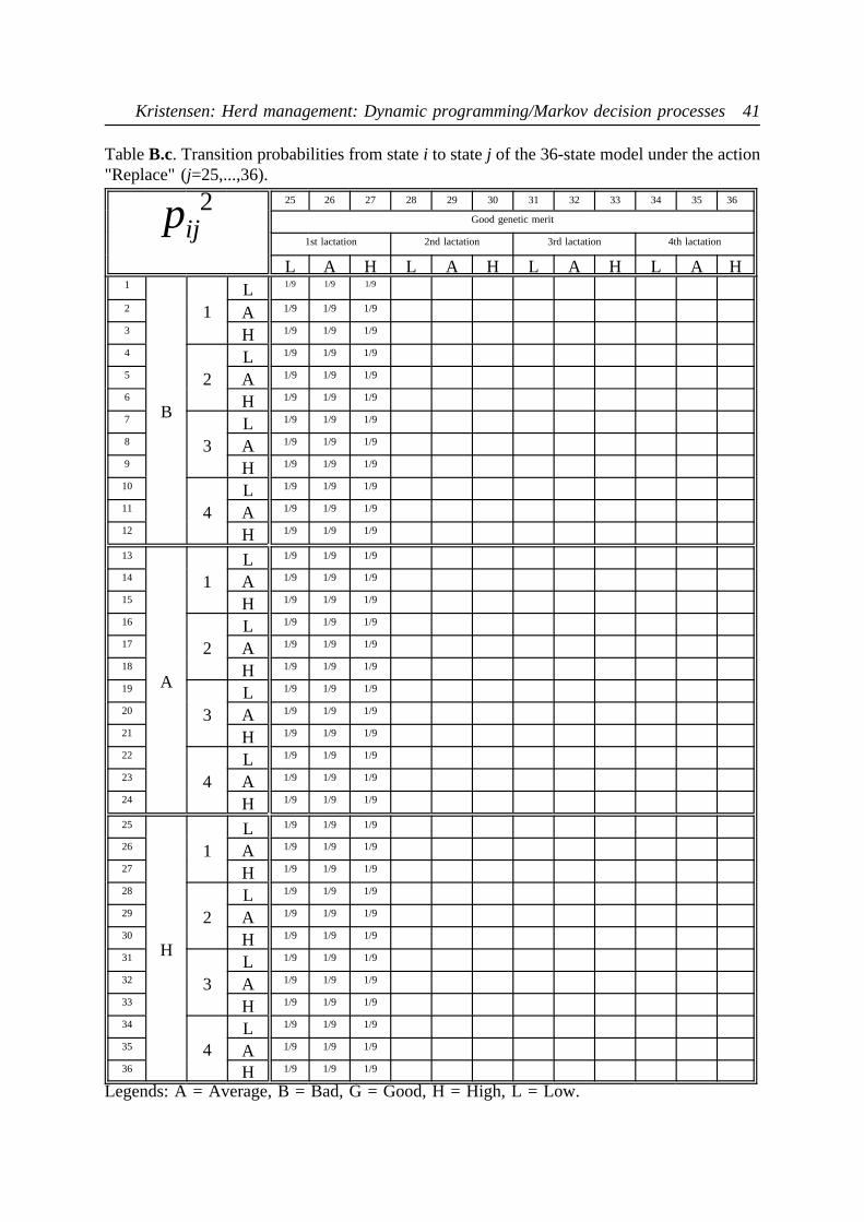
Kristensen: Herd management: Dynamic programming/Markov decision processes 41
TableB.c. Transition probabilities from statei to statej of the 36-state model under the action"Replace" (j=25,...,36).
pij2 25 26 27 28 29 30 31 32 33 34 35 36
Good genetic merit
1st lactation 2nd lactation 3rd lactation 4th lactation
L A H L A H L A H L A H1
B
1L 1/9 1/9 1/9
2 A 1/9 1/9 1/9
3 H 1/9 1/9 1/9
4
2L 1/9 1/9 1/9
5 A 1/9 1/9 1/9
6 H 1/9 1/9 1/9
7
3L 1/9 1/9 1/9
8 A 1/9 1/9 1/9
9 H 1/9 1/9 1/9
10
4L 1/9 1/9 1/9
11 A 1/9 1/9 1/9
12 H 1/9 1/9 1/9
13
A
1L 1/9 1/9 1/9
14 A 1/9 1/9 1/9
15 H 1/9 1/9 1/9
16
2L 1/9 1/9 1/9
17 A 1/9 1/9 1/9
18 H 1/9 1/9 1/9
19
3L 1/9 1/9 1/9
20 A 1/9 1/9 1/9
21 H 1/9 1/9 1/9
22
4L 1/9 1/9 1/9
23 A 1/9 1/9 1/9
24 H 1/9 1/9 1/9
25
H
1L 1/9 1/9 1/9
26 A 1/9 1/9 1/9
27 H 1/9 1/9 1/9
28
2L 1/9 1/9 1/9
29 A 1/9 1/9 1/9
30 H 1/9 1/9 1/9
31
3L 1/9 1/9 1/9
32 A 1/9 1/9 1/9
33 H 1/9 1/9 1/9
34
4L 1/9 1/9 1/9
35 A 1/9 1/9 1/9
36 H 1/9 1/9 1/9
Legends: A = Average, B = Bad, G = Good, H = High, L = Low.