Dynamic Pricing in a Labor Market: SurgePricing and Flexible Work on the Uber Platform

M. Keith Chen∗ and Michael Sheldon

December 11, 2015

Abstract

This paper studies how the dynamic pricing of tasks in the “gig” econ-omy influences the supply of labor. A large economic literature has ex-plored labor supply when workers can flexibly choose how long to workeach day. In a study of taxi drivers, Camerer et al. (1997) claim thatdrivers quit when they hit a daily income target, consequently drivingless when hourly earnings are high. If general, this behavior would under-mine the benefits of emerging “sharing economy” markets where tasks aredynamically priced. In this paper, we study how driver-partners on theUber platform respond to the dynamic pricing of trips, known as “surge”pricing. In contrast to income-target findings, we find that Uber partnersdrive more at times when earnings are high, and flexibly adjust to drivemore at high surge times. A discontinuity design confirms that these ef-fects are causal, and that surge pricing significantly increases the supplyof rides on the Uber system. We discuss the implications of these findingsfor earnings, flexible work, and the efficiency of dynamically-priced labormarkets.

∗Chen: UCLA Anderson, keith.chen@anderson.ucla.edu. Sheldon: University of Chicago,msx@uchicago.edu. Comments are welcome at keith.chen@anderson.ucla.edu. We thankFranziska Bell, Judith Chevalier, Jonathan Hall, Barry Nalebuff, Connan Snider, MollySpaeth, and seminar participants at Princeton, RAND, UCLA, and USC for generous feed-back and suggestions. All errors in this draft are the responsibility of the authors. Disclosures:Chen currently serves as the Head of Economic Research for Uber, where he designed the mostrecent surge algorithm. Sheldon held a summer internship at Uber. Keywords: labor supply,income targeting, dynamic pricing, ridesharing, two-sided markets, the sharing economy.

1

In many markets, new technologies allow traditional jobs to be divided into dis-crete tasks that are widely distributed across workers and dynamically pricedgiven prevailing supply and demand conditions. This “sharing” or “gig” econ-omy represents a shift away from fixed employment contracts to a more flex-ible work system, and is most common in two-sided markets in which a firmacts as a platform to connect service providers and consumers. One prominentexample of this is the ride-sharing company Uber, which connects riders anddriver-partners,1 and dynamically prices trips using a system known as “surge”pricing. While there is broad consensus among economists that platforms likeUber increases consumer welfare,2 less attention has been paid to its effects onthe labor market in terms of earnings, work flexibility, and overall efficiency.

In the case of Uber, qualified driver-partners earn fares by providing rideson the Uber platform, and can use the platform as much or as little as theywant. Drivers on the Uber platform enjoy hours flexibility, and must decideboth how much and when they wish to drive. Given this flexibility, a centralquestion is the extent to which firms can influence the supply of services ontheir platforms, particularly in the short term. Indeed, the income-targetingliterature would suggest that perversely, increasing the price of services mightactually decrease the supply of services on these platforms.

This paper aims to measure how the dynamic pricing of tasks on online“sharing” and “gig” economy platforms influence the supply of labor on theintensive margin.3 Central to this question are the characteristics of workers’labor supply elasticities; that is, the responsiveness of supply hours to changes inthe prevailing price of services. We measure and characterize these elasticities fordrivers on the UberX platform, and find significantly and substantially positivesupply elasticities. In addition, we find that increases in the “surge” price ofUber trips significantly decreases the instantaneous stopping rate of drivers onthe Uber platform. That is, drivers appear to dynamically adjust their schedulesto drive longer and provide more trips at times with high surge prices. Thissuggests that surge pricing significantly increases the number of trips that occur,and boosts the overall efficiency of the Uber system.

1 Supply Elasticities and Flexible WorkThere is a large empirical literature that studies the magnitude and direction oflabor supply elasticities. A substantial portion of the literature has found evi-

1As used in this paper, a ’driver-partner’ is someone who earns income providing rides onthe Uber platform.

2Surveys of prominent economists show broad agreement that platforms such as Uber ben-efit consumers: http://www.igmchicago.org/igm-economic-experts-panel/poll-results?SurveyID=SV_eyDrhnya7vAPrX7,

and that in particular, surge pricing accounts for some of these benefits:http://www.igmchicago.org/igm-economic-experts-panel/poll-results?SurveyID=SV_

2bC0xviyL9hsNLL.3Here we define the intensive labor margin is how much work a person decides to supply

conditional on deciding to work that day.

2

dence of positive supply elasticities, in line with standard theories of intertem-poral substitution of labor. These studies span a variety of markets includingconstruction work on the Trans-Alaskan pipeline (Carrington, 1996), stadiumvendors (Ottenginer, 1999), and lobster trappers/divers (Stafford, 2013).4 Insharp contrast to these studies however, Camerer, Babcock, Loewenstein, andThaler (1997) finds surprising evidence of negative earning elasticities in a studyof New York City cab drivers. Positing that taxi drivers choose their hours usingreference points, Camerer et al. justified these findings theoretically by devel-oping a theory of “income targeting”; the idea that a taxi driver has a dailyincome target, after which they are much more likely to stop providing rides.This results in drivers choosing to work more hours when pay is low, resulting innegative earnings elasticities. Though Camerer et al. has been an extremely in-fluential study, it has been controversial. Several subsequent papers have foundsupport for an income-targeting hypothesis, (Fehr and Goette 2002, Crawfordand Meng 2011, Chang and Gross 2014), while others have failed to find sup-porting evidence (Ottenginer 1999, Stafford 2013), and others have suggestedthat income-target findings are largely econometric artifacts (Farber 2005, 2008,2014).

Naturally, the direction of labor supply elasticities holds strong implicationsfor the effectiveness of a dynamic labor-pricing mechanism. Firms such as Uberpromote their dynamic pricing systems by claiming that higher fares not onlytemporarily lower demand but also raise supply by incentivizing drivers cur-rently off the platform to log-on and drivers already on the system to stay onlonger. To the extent that Uber partners systematically income target, the ef-fect of higher prices on aggregate supply may be muted or even negative. Thatis, surge pricing could push more supply off the system than on, potentially ex-acerbating the supply/demand imbalance. Therefore, determining the directionas well as the magnitude of high-frequency labor supply elasticities is funda-mental to the economic justification of not just Uber’s dynamic pricing system,but any firm employing a dynamic pricing system to incentivize the supply ofservices. Here, we study this question using data on Uber driver-partners andtheir response to surge pricing.

2 The Uber Marketplace and Surge Pricing

2.1 Overview of the Uber PlatformUber is a technology firm most well-known for managing a ride-sharing plat-form.5 Uber provides a mobile application which creates a two-sided marketfor on-demand transportation, primarily in metropolitan areas. Riders pay afare based on the distance of their trip and the time taken to complete the trip;

4For a detailed summary of the literature, see Farber (2008).5While Uber offers products outside of ridesharing, for example UberEATS (on-demand

meal delivery) and UberRush (on-demand courier service), we do not explore those productshere.

3

drivers receive this fare minus a service fee paid to Uber. Payments are remittedto drivers on a weekly basis, though the amount earned is known by the driverat the end of each trip.

In this study we focus on UberX, which in the United States is Uber’s peer-to-peer service. We study UberX not only because it is the most popular, butbecause characteristics of other products make them less amenable to study.For example, drivers on UberBlack are licensed commercial drivers, some ofwho work for limo companies and may be paid a fixed salary that does notrespond to surge pricing. Most have outside options which may covary withUber market conditions,6 making the interpretation of their time on and offthe Uber platform harder to interpret. The same criticism applies to uberTaxidrivers (taxi drivers who opt-in to the Uber platform), with the additionalcomplication that they can also pick up street hails and are not subject to surgepricing.

Because of these issues, we focus on driver-partners who supply rides exclu-sively on the UberX platform.7 As a platform, UberX possesses many qualitieswhich make it an ideal setting in which to analyze intensive supply elasticities.Scheduling flexibility is a feature of driving on the Uber platform; unlike mostworkers in the U.S. economy, UberX partners face no explicit constraints onwhen they can work. Conditional on qualifying to drive, an UberX partner canfreely choose the days and hours they are active on the platform.8 Further-more, in contrast to the taxi industry, short term vehicle leases are not typical;most UberX partners own and control their own vehicles. These characteristicsavoid much of the “constrained hours” problems with measuring labor-supplyelasticities in more traditional labor markets.

2.2 The Surge-Pricing MechanismThe Uber platform adjusts its prices using a realtime dynamic algorithm knownas “Surge” pricing, which has generated considerable interest among both thepress and academics.9 Surge pricing is the output of an algorithm which au-tomatically raises the price of a trip when demand outstrips supply within afixed geographic area. Trip prices are adjusted by multiplying the prices of theunderlying components which make up fare –the base fare, the price per mile,and the price per minute–10 by a multiplier output by the surge algorithm. Thismultiplier is communicated to both riders and partners before each trip is initi-ated; riders see and must confirm, the surge multiplier (SM) before requesting

6UberBlack drivers may display muted earnings elasticities if low-demand conditions (lowhourly earnings on Uber) correlate to low rates of commercial bookings and vice versa.

7Drivers can be affiliated with multiple products; for example, both UberX and UberBlack.We exclude such drivers from the analysis.

8For an excellent summary of what we know about the characteristics of Uber driver-partners, see Hall and Kruger 2015.

9See Chen et al. for an early analysis of surge pricing.10There are some components of a fare which are fixed and not affected by the surge mul-

tiplier, such as the “Safe Rides Fee”. These fixed fees do not increase with surge, and are notare not remitted to the partner.

4

a pick-up. Partners are informed of the current surge multiplier in an area bothwhen they are offered a pickup and also through heat-maps displayed on thepartner’s mobile application (See Figure 3 below).

Surge multipliers are discrete; they range from a minimum of 1.2 up to a city-specific maximum in increment of 0.1. The specific multiplier is determined atany given time by what will be referred to as a generator surge multiplier (GSM),a continuous value from which the implemented surge multiplier is derived from,typically by rounding to the nearest tenth. One can think of the GSM as Uber’sestimate of the “true” market price for rides at a point in space and time, whilethe SM is the implemented price. There are a several rules applied to thegeneration of the SM from the GSM, such as maximum step sizes (how muchthe SM can increase or decrease from its last value) or absolute caps (a city mayplace a cap of 2.9 on SMs, for example). In general, unless one of these specialcircumstances applies the SM is the GSM, rounded to the nearest tenth. Thisdistinction is not important for the majority of the analysis, but does play animportant role in Section 4.1 when we use the rounding of GSMs into SMs asan source of identification.

3 Data and MethodsOur data represent a randomly-drawn subset of UberX partners in Chicago,Washington DC, Miami, San Diego, and Seattle. For these partners, we observeever trip they provided on the Uber platform between September 4th, 2014, andJuly 4th, 2015. This comprises roughly 25 million trips.

3.1 Categorization of SessionsA unique challenge of this dataset is the conceptualization of a partner’s “work-day” or “shift”. In contrast to papers studying the labor supply of taxi drivers,the lack of organizational constraints on time worked implies that the supplychoices of Uber partners need not resemble a typical workday. While this flexibil-ity provides driver-partners with a clear benefit, it poses an analytic challenge indefining the correct unit of time for analysis, particularly for an income-targetinghypothesis.

An intuitive first approach would be to study the decision as to how manyhours a driver-partner decides to supply per calendar day. However, this ap-proach splits in two any driving session which crosses over midnight–which,particularly on weekends, are times at which many Uber partners choose todrive. A modified but similar approach is used by Farber (2014) in his analysisof New York City taxi drivers; instead of separating a day at midnight he definesa day transition at 4AM, the time of day with the lowest number of drivers onthe road.

Here, we analyze Uber partner choices using a flexible session-based approachwhich ameliorates many of these potential biases. We define a session as thecluster of all trip and application activity that occur without a break of more

5

than 4 hours. That is, a period of partner inactivity greater than four hoursmarks the beginning of a new session in the data. Conceptually, the use of afour-hour gap allows partners to take short breaks for meals or errands withoutcounting such breaks as ending a session. The “length” of a session is defined asthe total time that the driver is on-app in a session, either serving a ride request,or online and available to accept a trip dispatch. Given these definitions wethen examine the determinants of both session length and the decision to end asession.11

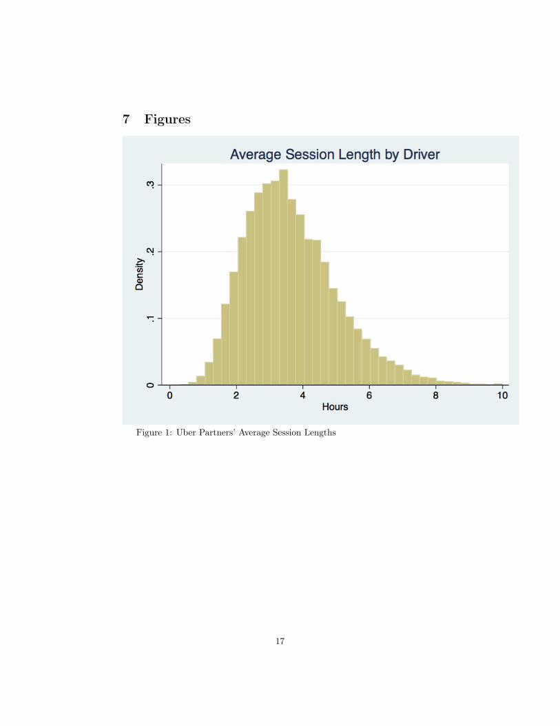
Figures 1 and 2 below show the average length of session per driver-partner,and how much each partner’s sessions deviate from their average session length.12Uber driver-partners tend to drive multiple short rather than fewer long sessions,with most sessions ranging between 2 and 5 hours, and the median driver aver-aging 3.47 hours per session. As figure 2 shows, session lengths also vary widelywithin driver. In our sample, roughly 5% of a partner’s sessions are more thantwice as long as their average session, and over 18% are less than half theiraverage. This suggests that Uber driver-partners regularly take advantage ofthe platform’s work flexibility. We now examine the degree to which partnersuse this flexibility to respond to both predictable and unpredictable changes inthe price of trips.

4 Results

4.1 Autocorrelation of IncomeAs Farber (2005) notes, current income is only a rational input to supply de-cisions if it significantly predicts (immediate) future earnings. That is, yourcurrent income rate should only influence your decision to keep driving if itmeaningfully predicts expected earnings going forward. To verify this interpre-tation of the effect of current income on supply decisions within our models,we examine the inter-temporal properties of earnings by calculating autocorre-lations of the hourly city earnings.13 These are summarized in Table 1.

Average hourly earnings are highly correlated across hours within city in ourdataset. Though the degree of autocorrelation varies by city, in all cases it issignificant and substantially positive. These findings suggest that current earn-ings are informative of future opportunities, and that partners can use currentearnings as a proxy for future earnings over reasonable time frames.

11In a supplementary analysis we examine the sensitivity of our results to this definition ofa “session”, and find our results are both qualitatively and quantitatively robust. Under thisdefinition, our data are comprised of roughly 2.4 million sessions.

12Session length is measured as the amount of on-app time within a session. So for example,if during a session from 1 to 6pm a partner takes a 1 hour break and logs off the app, thatsession would be measured as 4 hours long.

13Here, “hourly city earnings” are the average hourly earnings for partners active in the city.

6

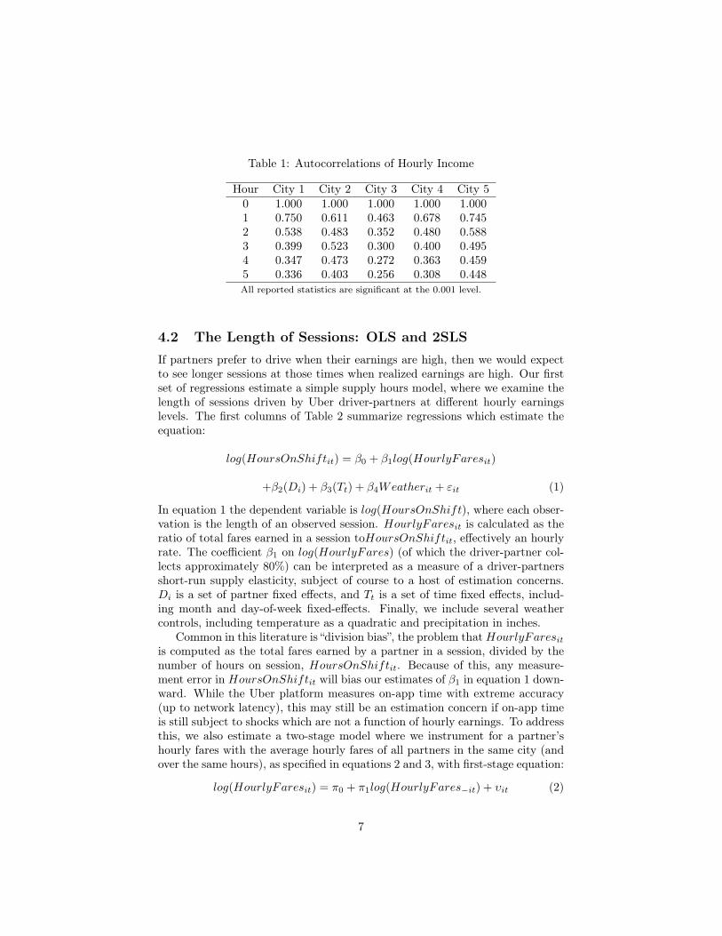
Table 1: Autocorrelations of Hourly Income

Hour City 1 City 2 City 3 City 4 City 50 1.000 1.000 1.000 1.000 1.0001 0.750 0.611 0.463 0.678 0.7452 0.538 0.483 0.352 0.480 0.5883 0.399 0.523 0.300 0.400 0.4954 0.347 0.473 0.272 0.363 0.4595 0.336 0.403 0.256 0.308 0.448All reported statistics are significant at the 0.001 level.

4.2 The Length of Sessions: OLS and 2SLSIf partners prefer to drive when their earnings are high, then we would expectto see longer sessions at those times when realized earnings are high. Our firstset of regressions estimate a simple supply hours model, where we examine thelength of sessions driven by Uber driver-partners at different hourly earningslevels. The first columns of Table 2 summarize regressions which estimate theequation:

log(HoursOnShiftit) = β0 + β1log(HourlyFaresit)

+β2(Di) + β3(Tt) + β4Weatherit + εit (1)

In equation 1 the dependent variable is log(HoursOnShift), where each obser-vation is the length of an observed session. HourlyFaresit is calculated as theratio of total fares earned in a session toHoursOnShiftit, effectively an hourlyrate. The coefficient β1 on log(HourlyFares) (of which the driver-partner col-lects approximately 80%) can be interpreted as a measure of a driver-partnersshort-run supply elasticity, subject of course to a host of estimation concerns.Di is a set of partner fixed effects, and Tt is a set of time fixed effects, includ-ing month and day-of-week fixed-effects. Finally, we include several weathercontrols, including temperature as a quadratic and precipitation in inches.

Common in this literature is “division bias”, the problem thatHourlyFaresitis computed as the total fares earned by a partner in a session, divided by thenumber of hours on session, HoursOnShiftit. Because of this, any measure-ment error in HoursOnShiftit will bias our estimates of β1 in equation 1 down-ward. While the Uber platform measures on-app time with extreme accuracy(up to network latency), this may still be an estimation concern if on-app timeis still subject to shocks which are not a function of hourly earnings. To addressthis, we also estimate a two-stage model where we instrument for a partner’shourly fares with the average hourly fares of all partners in the same city (andover the same hours), as specified in equations 2 and 3, with first-stage equation:

log(HourlyFaresit) = π0 + π1log(HourlyFares−it) + υit (2)

7

Table 2: The Determinants of Session Length

OLS 2SLSVariables: (1) (2) (3) (4) (5) (6)

Log Own Income 0.145*** 0.197*** 0.168***(0.00144) (0.00258) (0.00261)

Log Average Income 0.292*** 0.585*** 0.503***(0.00237) (0.00518) (0.00565)

Constant 1.194*** 1.244*** 1.341*** 1.338*** 1.622*** 1.671***(0.00156) (0.00251) (0.00628) (0.00237) (0.00504) (0.00783)

Weather Controls X X

Fixed Effects:Partner X X X XMonth and Day of Week X XObservations 2,377,210 2,377,210 2,368,340 2,377,210 2,377,210 2,368,340Number of Partners 63,830 63,830 63,830 63,830 63,830 63,830R2 0.007 0.013 0.038

All regressions are OLS and 2SLS regressions with Log(Session Length) as the dependant variable.We report robust standard errors in parentheses; *** p<0.01, ** p<0.05.

and second-stage equation:

log(HoursOnShiftit) = β0 + β1log(HourlyFaresit)

+β2(Di) + β3(Tt) + β4Weatherit + εit (3)

The results for both the OLS method (Specifications 1-3) and the 2SLSmethod (Specifications 4-6) are given in Table 2. Specification 1 includes nocontrols and provides an elasticity significantly and substantially greater thanzero, approximately 0.15. Controlling for partner fixed effects in specification 2increases this elasticity slightly, which decreases again in specification 3 whencalendar effects (month of year and day of week, separately) and weather (tem-perature in quadratic terms and precipitation totals) are added, resulting inan elasticity of about 0.17. The results from the fixed-effects (omitted here)indicate that differences between partners are significant, that partners providemore hours on the weekend, and drive less hours in response to rain or extremetemperatures.

Given the “division bias” we discuss above, we rerun the specifications in 1-3as a two-stage model in 4-6 using the average hourly income of all partners in thesame city (and over the same hours) as an instrument for a partner’s own hourlyincome. The specifications progress in levels of fixed effects in the same manner

8

as the OLS estimates. Compared to the OLS estimates, the 2SLS estimates aresubstantially higher; more than doubling the corresponding OLS estimates inall cases and resulting in a supply elasticity of approximately 0.50. This increaseis consistent with the concern that OLS estimates may be downwardly biaseddue to measurement error in HoursOnShiftit.

It should be noted that the effect of instruments on our estimates, whilesubstantial, is considerably less than in Camerer (1997) or Farber (2005). Thisis likely because Uber data is measured by a smartphone and displays less mea-surement error in active-session time. These elasticities are consistently bothstatistically and economically positive, so do not support the income-targetinghypothesis proposed in Camerer et al. (1997). We find that partners work longerhours when the earnings are high, and that higher prices stimulate supply onthe intensive margin.

4.3 Ending a Session: Modeling the Decision to StopOur first analysis closely follows the existing literature, but like those paperssuffers from an endogeneity problem that is difficult to overcome within a work-hours framework. Earnings levels in the Uber environment are driven by shocksto both demand and supply; and when earnings variation is driven by sup-ply, it is likely that both outside options and/or opportunity costs for partnersare strongly correlated with earnings. Therefore β1 can not be unambiguouslyinterpreted as an income elasticity.

Our second analysis focuses on estimating the effect of unexpected shocks toearnings, as driven by the Surge Multiplier, on a partner’s decision to continueor stop driving within a session. To study this decision, we study the predictorsof a trip ending a session. We take the Surge Multiplier that is in effect inthe location where a partner ends a trip, as the best proxy for the earningsthey should expect should they continue driving. Additional controls includecumulative measures of their session (fare, time, distance traveled, and numberof trips), and current weather conditions. Conceptually, we are gauging howthese factors affect a partner’s decision to continue driving after each trip.

9

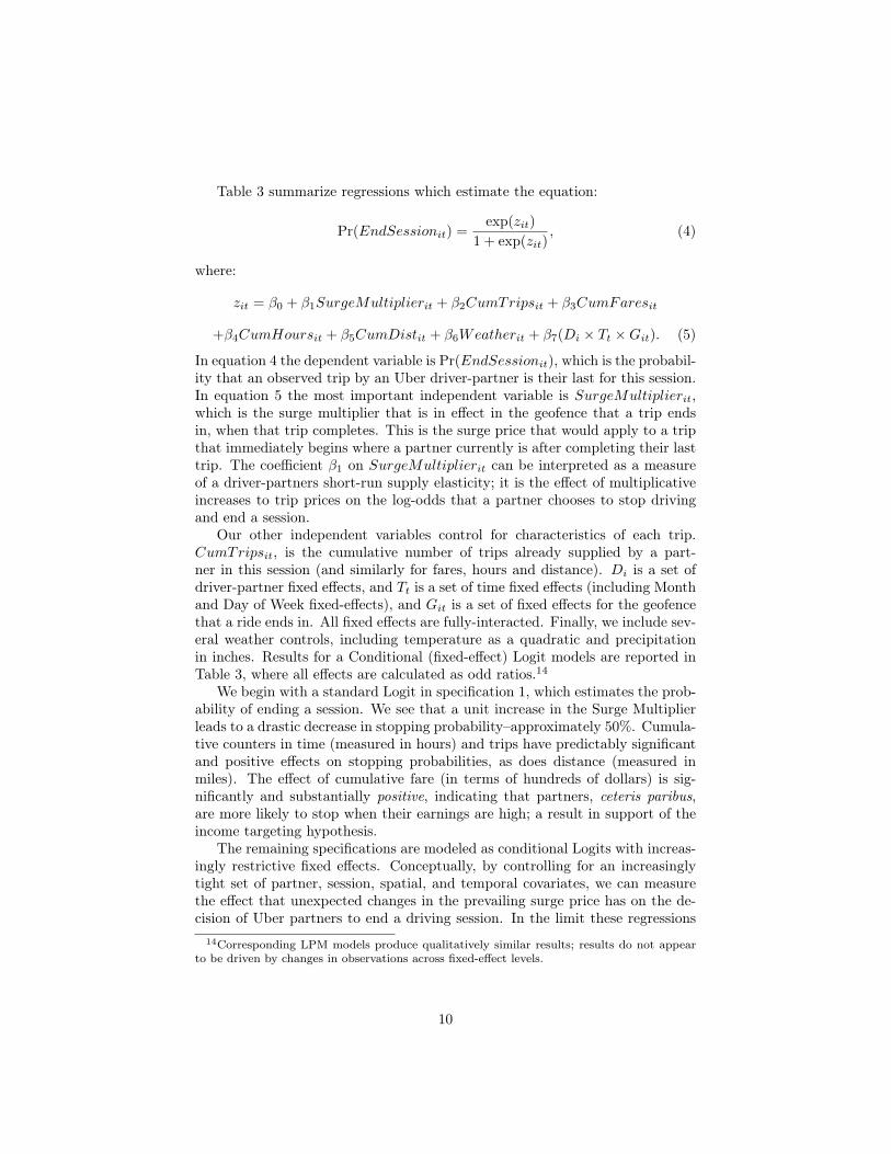
Table 3 summarize regressions which estimate the equation:

Pr(EndSessionit) =exp(zit)

1 + exp(zit), (4)

where:

zit = β0 + β1SurgeMultiplierit + β2CumTripsit + β3CumFaresit

+β4CumHoursit + β5CumDistit + β6Weatherit + β7(Di × Tt ×Git). (5)

In equation 4 the dependent variable is Pr(EndSessionit), which is the probabil-ity that an observed trip by an Uber driver-partner is their last for this session.In equation 5 the most important independent variable is SurgeMultiplierit,which is the surge multiplier that is in effect in the geofence that a trip endsin, when that trip completes. This is the surge price that would apply to a tripthat immediately begins where a partner currently is after completing their lasttrip. The coefficient β1 on SurgeMultiplierit can be interpreted as a measureof a driver-partners short-run supply elasticity; it is the effect of multiplicativeincreases to trip prices on the log-odds that a partner chooses to stop drivingand end a session.

Our other independent variables control for characteristics of each trip.CumTripsit, is the cumulative number of trips already supplied by a part-ner in this session (and similarly for fares, hours and distance). Di is a set ofdriver-partner fixed effects, and Tt is a set of time fixed effects (including Monthand Day of Week fixed-effects), and Git is a set of fixed effects for the geofencethat a ride ends in. All fixed effects are fully-interacted. Finally, we include sev-eral weather controls, including temperature as a quadratic and precipitationin inches. Results for a Conditional (fixed-effect) Logit models are reported inTable 3, where all effects are calculated as odd ratios.14

We begin with a standard Logit in specification 1, which estimates the prob-ability of ending a session. We see that a unit increase in the Surge Multiplierleads to a drastic decrease in stopping probability–approximately 50%. Cumula-tive counters in time (measured in hours) and trips have predictably significantand positive effects on stopping probabilities, as does distance (measured inmiles). The effect of cumulative fare (in terms of hundreds of dollars) is sig-nificantly and substantially positive, indicating that partners, ceteris paribus,are more likely to stop when their earnings are high; a result in support of theincome targeting hypothesis.

The remaining specifications are modeled as conditional Logits with increas-ingly restrictive fixed effects. Conceptually, by controlling for an increasinglytight set of partner, session, spatial, and temporal covariates, we can measurethe effect that unexpected changes in the prevailing surge price has on the de-cision of Uber partners to end a driving session. In the limit these regressions

14Corresponding LPM models produce qualitatively similar results; results do not appearto be driven by changes in observations across fixed-effect levels.

10

Table 3: The Choice to End a Driving Session: Conditional Logits

Conditional (Fixed-Effect) Logistic RegressionVariables: (1) (2) (3) (4)

Surge Multiplier 0.516*** 0.512*** 0.565*** 0.700***(0.00129) (0.00132) (0.00163) (0.00275)

C. Trips 0.955*** 1.033*** 1.008*** 1.039***(0.000208) (0.000310) (0.000375) (0.000553)

C. Fare (hundreds) 1.248*** 1.091*** 1.000 0.957***(0.00144) (0.00212) (0.00249) (0.00361)

C. Time (hours) 1.176*** 1.156*** 1.110*** 1.119***(0.000504) (0.000602) (0.000722) (0.00105)

C. Distance (miles) 1.003*** 1.010*** 1.009*** 1.003***(4.02e-05) (5.91e-05) (7.28e-05) (0.000111)

Precipitation (inches) 0.951 0.876*** 1.036 0.797***(0.0292) (0.0287) (0.0405) (0.0473)

Temperature 0.999*** 1.006*** 1.005*** 1.008***(0.000175) (0.000208) (0.000240) (0.000330)

Temperature2 1.000*** 1.000*** 1.000*** 1.000***(1.64e-06) (1.96e-06) (2.29e-06) (3.22e-06)

Constant 0.124***(0.000344)

Fixed Effects:PartnerxDay XPartnerxDayxHour XPartnerxDayxHourxGeo XObservations 25,056,304 23,633,812 14,021,328 5,234,517

We report coefficients as odds-ratios and robust standard errors in parentheses.*** p<0.01, ** p<0.05, * p<0.1.

11

estimate the degree to which an increase in surge prices and hence per-trip earn-ings, causally induces Uber driver-partners to provide more rides on the Uberplatform.

Column 2 includes Partner x Day of Week fixed effects, controlling for theeffect of a particular partner on a particular day of week. Most variables of inter-est remain remarkably similar– responses to surge multiplier, time, and distanceare negligible. The impact of cumulative fare diminishes substantially, losingover half of its magnitude; however, it still remains significant and economicallysubstantial in influencing a partner’s decision to stop.

Specification 3 narrows the fixed effect further to the interaction of Partnerx Day x Hour ; defining groups of observations which have multiple entries forthe same partner, day of week, and hour of day. This fixed effect is quiterestrictive, and as such the number of observations our model can use decreasessubstantially;15 nevertheless the results and still highly significant and theirinterpretation meaningful. Coefficients for time, distance, and trips alter slightlybut not neither substantially nor meaningfully. The effect of the surge multiplierdecreases slightly, but still remains quite powerful. Interestingly, the effect ofcumulative fare goes to 0, suggesting that the evidence in favor of the incometargeting hypothesis is not robust to model specification.

Specification 4 provides an even more aggressive level of fixed effect, Part-ner x Day x Hour x Geozone. Conceptually, we are grouping observations byindividual partner, day of week, hour of day, and region of city where they endthe trip. That is, we are only comparing trips that the same partner endedon a Monday, between 2 and 3, in this neighborhood. Sample size decreasesdrastically but remains sizable. Coefficients for time, distance, and trips remainsimilar. The impact of surge multiplier again decreases, and this time by amuch greater magnitude, but remains a powerful, negative effect on stoppingprobability. Cumulative fare now has a negative impact on stopping probability–provided the same interpretation holds on cumulative as in the previous analysis,this implies partners are less likely to stop when earnings are high. Thus, theresults with respect to the impact of income on a partner’s decision to stop areconsistent with the results above and neoclassical models of labor supply, anddo not support the income-targeting hypothesis.

The impact the level of fixed effects have on the model highlights the powerfulspatiotemporal influences that are involved with a partner’s decisions–failure toaccurately capture these effects amounts to a potentially large source of bias inthe estimation. The trend in coefficients displayed here tells a very compellingstory– given a higher set of prices, partners will choose to work more than theyotherwise would have. Thus, changes in the surge multiplier directly effect thesupply decisions of partners even after they have decided to drive on a givenday. Furthermore, the coefficient on cumulative fare suggests that the SurgeMultiplier does not even indirectly encourage supply churn by allowing partnersto hit “income targets” sooner. Rather, since partners react to higher cumulative

15The conditional Logit model requires at least one observation of each outcome within eachfixed-effect group.

12

incomes by driving longer, surge multipliers appear to have a secondary, positiveeffect on labor supply through increasing incomes. Overall, it appears that thedynamic pricing mechanism is very effective in encouraging short-term supplygrowth on the Uber platform by encouraging partners already on the system tocontribute more time than they otherwise would have.

4.4 Stopping Model with Running VariableOne concern about the results presented thus far is that, even given the stronglevel of fixed effects and controls already imposed, there may be underlyingunobserved elements driving both the change in surge multiplier and a partner’sdecision to stop; thus, the effect of the surge multiplier may be biased. InTable 4, we run the same conditional Logit models as above, but this timewith a high-order polynomial in the Generator Surge Multiplier–the continuousnumber which the surge multiplier is rounded from.

By including both the SM and the GSM in the same model, the coefficientof the surge multiplier regressor can be interpreted as the average, direct impactof an increase–akin to a regression discontinuity design. That is, the high ordergenerating variable should control all underlying covariates provided they donot jump discontinuously with surge prices, allowing these regressions to isolatethe pure effect of the surge multiplier. The results in Table 4 suggest that surgemultipliers exerts a powerful effect on the stopping probabilities of partners evenunder the most stringent of controls. The decrease in this effect compared tothe results in Table 3 for the corresponding models can be attribute to changesin demand conditions within surge multiplier.

5 DiscussionThe results presented here demonstrate the effect of increased earnings on thesupply decisions of partners. In contrast to the income-targeting literature, wefind that in response to surge pricing, Uber driver-partners choose to extendtheir sessions and provide significantly more rides on the Uber platform. Thisfinding remains sizable even with the inclusion of extremely aggressive part-ner, session, spatial, and temporal controls. These controls, plus the inclusionof the generator surge multiplier, allow us to measure the supply elasticity ofUber partners in response to unexpected changes in earnings as driven by un-predictable variation in surge pricing.

Our findings suggest that Uber partners both drive at times with higher de-mand for rides, and dynamically extend their sessions when surge pricing raisesearnings. In contrast to the existing literature, we find that Uber driver-partnersdo not display behavior consistent with income-targeting. These findings runcontrary to a large literature on the behavior of cab drivers, which found evi-dence that taxi drivers reduce the supply of rides when demand is unexpectedlyhigh. Those effects, if they held in the case of Uber surge pricing, would havesignificantly reduced the economic gains from dynamic pricing. To the contrary,

13

Table 4: Stopping Probabilities with a GSM Running Variable Control

Conditional (Fixed-Effect) Logistic RegressionVariables: (1) (2) (3)

Surge Multiplier 0.730*** 0.774*** 0.805***(0.00458) (0.00564) (0.00865)

GSM: 5th Order Poly.

C. Trips 1.044*** 1.017*** 1.042***(0.000354) (0.000431) (0.000624)

C. Fare (hundreds) 1.148*** 1.033*** 0.989**(0.00256) (0.00300) (0.00433)

C. Time (hours) 1.144*** 1.103*** 1.107***(0.000679) (0.000823) (0.00118)

C. Dist. (miles) 1.008*** 1.007*** 1.003***(6.91e-05) (8.61e-05) (0.000128)

Precipitation (inches) 1.068* 1.304*** 1.019(0.0406) (0.0595) (0.0708)

Temperature 1.001*** 1.000* 1.004***(0.000233) (0.000271) (0.000369)

Temperature2 1.000*** 1.000*** 1.000***(2.23e-06) (2.61e-06) (3.64e-06)

Fixed Effects:PartnerxDay XPartnerxDayxHour XPartnerxDayxHourxGeo XObservations 19,051,247 10,599,081 4,112,257We report coefficients as odds-ratios and robust standard errors in parentheses.

*** p<0.01, ** p<0.05, * p<0.1.

14

we find large and pervasive positive supply elasticities, suggesting that dynamicpricing, at least in the case of Uber, significantly increases the efficiency of theride-sharing market.

That we do not find income-targeting on the session-hours level is particu-larly surprising since this analysis is extremely similar to the seminal Camerer etal. and the literature that followed it. While we do not directly reanalyze theirdata, one possible explanation of this discrepancy is that we have extremely pre-cise measurements of Uber partners’ time on session; Farber emphasizes thatmeasurement error in this variable has the ability to produce spurious income-targeting findings (Farber 2005, 2008). Another possibility is that on the Uberplatform, earnings variation arises through extremely salient surge-induced in-creases in earnings-per-trip, rather than indirect earnings fluctuations throughtrip frequency, as in taxi markets. Finally, Uber partners interact with the plat-form through a smartphone interface that allows them to know current pricesand session statistics like cumulative earnings, time, and trips (see Figure 3 foran example screenshot). It is possible that with access to more and more easilyorganized information, Uber driver-partners need not rely on rules of thumb likea daily income target.

Finally, our work is one of the first to document the degree to which platformssuch as Uber enable extremely flexible work schedules, and the degree to whichUber driver-partners take advantage of that flexibility. Even under a generous4-hour break definition, the median driver-partner averages less than three anda half hours per session, and varies that session length considerably to takeadvantage of surge pricing. To the degree that the “sharing economy” promisesgreater work flexibility, Uber driver-partners appear to take advantage of thatflexibility in ways that increase their hourly earnings.

6 ConclusionOverall, our findings support the idea that dynamic pricing significantly in-creases the efficiency of on-demand service markets. On the Uber platformsurge pricing appears to increase the supply of rides on the Uber platform byincentivising driver-partners to provide more rides than they would have ab-sent surge prices. We find evidence that this happens both immediately (byimmediately lengthening sessions), as well as the longer time frames over whichdriver-partners plan their session schedules. While we investigate data on onlythe Uber platform, our findings suggest that dynamic pricing could significantlyincrease the efficiency of many of emerging “gig” markets where jobs are widelydistributed across workers and in which prevailing market conditions can fluc-tuate across both time and location.

15

References[1] Camerer, Colin; Linda Babcock; George Loewenstein; and Richard Thaler,

“Labor Supply of New York City Cabdrivers: One Day at a Time,” Quar-terly Journal of Economics 112 (May 1997), pp. 407 – 441.

[2] Chang, Tom and Tal Gross. “How many pears would a pear packer pack ifa pear packer could pack pears at quasi-exogenously varying piece rates?”Journal of Economic Behavior and Organization 99 (2014) pp. 1-17.

[3] Chen, Le; Alan Mislove; and Christo Wilson, “Peeking Beneath the Hood ofUber,” Proceedings of the 2015 ACM Conference on Internet MeasurementConference, pp. 495-508.

[4] Crawford, Vincent P. and Juanjuan Meng. “New York City Cab DriversLabor Supply Revisited: Reference-Dependent Preference with RationalExpectations Targets for Hours and Income,” American Economic Review101 (2011) pp. 1912-1932.

[5] Hall Jonathan V. and Alan B. Krueger. “An Analysis of the Labor Mar-ket for Uber’s Driver-Partners in the United States,” Princeton UniversityWorking Papers Industrial Relations Section, (2015), #587.

[6] Farber, Henry S. “Is Tomorrow Another Day? The Labor Supply of NewYork City Cab Drivers,” Journal of Political Economy 113 (February 2005),pp. 46-82.

[7] Farber, Henry S. “Reference-Dependent Preferences and Labor Supply: TheCase of New York City Taxi Drivers,” American Economic Review 98 (June2008), pp. 1069-1082.

[8] Farber, Henry S. “Why You Can’t Find a Taxi in the Rain and Other LaborSupply Lessons from Cab Drivers,” Princeton University Working PapersIndustrial Relations Section, (2014), #583b.

[9] Fehr, Ernst and Lorenz Goette. “Do Workers Work More if Wages are High?Evidence from a Randomized Field Experiment,” American Economic Re-view, 97(1) (2007) pp. 298-317.

[10] Oettinger, Gerald S. “An Empirical Analysis of the Daily Labor Supplyof Stadium Vendors,” Journal of Political Economy 107 (April 1999), pp.360-392.

16

7 Figures

Figure 1: Uber Partners’ Average Session Lengths

17

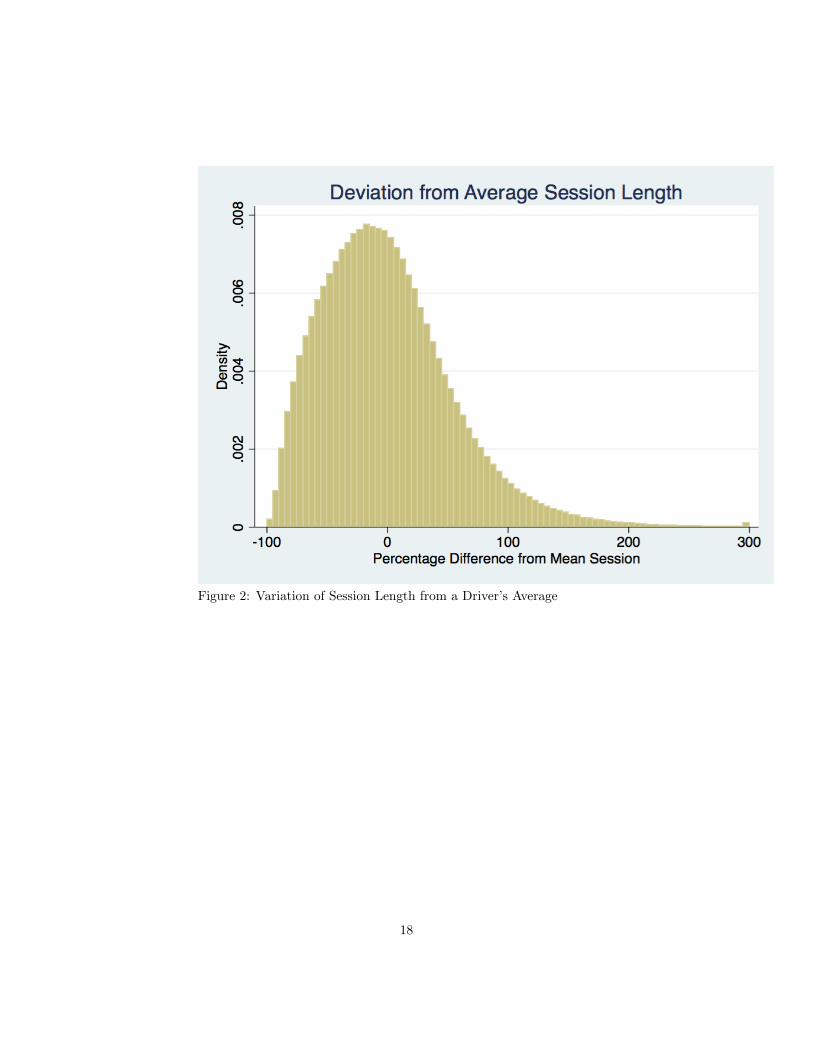
Figure 2: Variation of Session Length from a Driver’s Average

18

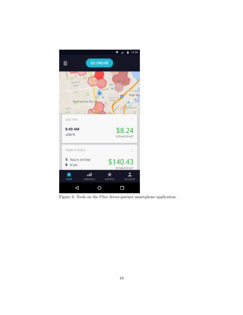
Figure 3: Tools on the Uber driver-partner smartphone application.

19