dynamic positioning of ships - semantic scholar · pdf file · 2015-09-23dynamic...
TRANSCRIPT
Dynamic Positioning of ShipsA nonlinear control design study
Proefschrift
ter verkrijging van de graad van doctoraan de Technische Universiteit Delft,
op gezag van de Rector Magnificus prof. ir. K.C.A.M Luyben,voorzitter van het College voor Promoties,
in het openbaar te verdedigen op maandag 23 april 2012 om 12:30 uur
door
Shah MUHAMMAD,Master of Science in Mathematics
Islamia University Bahawalpur, Pakistan
geboren te Dhurnal, Talagang, Pakistan.

Dit proefschrift is goedgekeurd door de promotor:Prof. dr. ir. A.W. Heemink
Copromotor:Dr. J.W. van der Woude
Samenstelling promotiecommissie:
Rector Magnificus voorzitterProf. dr.ir. A.W. Heemink Technische Universiteit Delft, promotorDr. J.W. van der Woude Technische Universiteit Delft, copromotorProf. dr.ir. J.H. van Schuppen Centrum Wiskunde & Informatica (CWI), AmsterdamProf. dr.ir. R.H.M. Huijsmans Technische Universiteit DelftProf. dr.ir. B. De Schutter Technische Universiteit DelftProf. dr.ir. R.L.M. Peeters Maastricht UniversityDr. A. Doria-Cerezo Univesitat Politecnica de Catalunya, Barcelona
This thesis has been completed in partial fulfillment of the requirements of Delft Uni-versity of Technology, The Netherlands, for the award of the PhD degree. The researchpresented in this thesis was supported in part by two institutions: Delft University ofTechnology and HEC Pakistan. I thank them sincerely for their support.
Published and distributed by: Shah MuhammadE-mail: [email protected]
Keywords: Dynamic positioning, Nonlinear control design, State dependent alge-braic Riccati equations, port-Hamiltonian systems.
ISBN # 978-94-6186-026-2Copyright© 2012 by Shah Muhammad
All rights reserved. No part of the material protected by this copyright notice maybe reproduced or utilized in any form or by any means, electronic or mechanical,including photocopying, recording or by any information storage and retrieval system,without written permission of the author.
The cover design is done by Fay van leeuwen: [email protected] in The Netherlands by Wohmann Print Service

iii
I want to dedicate this piece of work to my late father Dil Kabeer who realized thevalue of education for his kids and my beloved wife and kids, Hamael, Ashhal,
Bazeed, and Ehab for their consistent love and endurance.
The fate of each man We have bound about his neck. On the Day of Resurrection Weshall confront him with a book spread wide open, saying: ”Here is your book: read it.Enough for you this day that your own soul should call you to account.”
The Quran (Verses 13 and 14 from the chapter The Children of Israel)
ميقمہپ ايرثجواںوہہکںيہبسوتےتہاچميلس بلق ےرکوت اديپ ئوکاسيوےلہپ
لابقادمحمہمالع
ےہیہيتيریکیترهدسا،ےہرگنرواہي؛یجءاشنادناچےنپاےنپاےکبس،ںيهکنآینپاینپایکبس
ءاشنانباناخدمحمريش

iv
Contents
1 Introduction 11.1 What is a Dynamic Positioning (DP) System? . . . . . . . . . . . . . 1
1.1.1 Applications of DP Systems . . . . . . . . . . . . . . . . . . 21.1.2 Focus of this Research . . . . . . . . . . . . . . . . . . . . . 3
1.2 An Overview of this Thesis . . . . . . . . . . . . . . . . . . . . . . . 51.3 Contributions of this Thesis . . . . . . . . . . . . . . . . . . . . . . . 5
2 Mathematical Model of a Sea Vessel 72.1 Motion of a floating Vessel . . . . . . . . . . . . . . . . . . . . . . . 72.2 Mathematical Model Describing the Dynamics of a floating Vessel . . 9
2.2.1 The Dynamical Equations of Motion of the Vessel . . . . . . 102.2.2 The Disturbances Model . . . . . . . . . . . . . . . . . . . . 132.2.3 The Measurement Model . . . . . . . . . . . . . . . . . . . . 162.2.4 Wave Filtering . . . . . . . . . . . . . . . . . . . . . . . . . 16
2.3 Summary of the Mathematical Model . . . . . . . . . . . . . . . . . 172.4 Properties of the Model . . . . . . . . . . . . . . . . . . . . . . . . . 18
3 SDC Parametrization and Stability Analysis of Autonomous NonlinearSystems 213.1 State Dependent Coefficient Parametrization . . . . . . . . . . . . . . 213.2 Local Asymptotic Stability Analysis . . . . . . . . . . . . . . . . . . 233.3 Global Asymptotic Stability Analysis . . . . . . . . . . . . . . . . . 243.4 Exponential Boundedness and Global Asymptotic Stability . . . . . . 25
3.4.1 A Counterexample Showing that the Exponential Bounded-ness of the System Matrix does not Guarantee Global Asymp-totic Stability . . . . . . . . . . . . . . . . . . . . . . . . . . 25
3.5 Periodicity and Global Asymptotic Stability . . . . . . . . . . . . . . 283.5.1 A Counterexample Showing that the Periodicity of the System
Matrix does not Guarantee Global Asymptotic Stability . . . . 293.6 An LMI Based Approach for Global Asymptotic Stability . . . . . . . 33
3.6.1 Infeasibility of the LMI Feasibility Problem . . . . . . . . . . 38
v
vi Contents
3.6.2 Further Analysis for Global Asymptotic Stability . . . . . . . 423.7 Summary and Conclusions . . . . . . . . . . . . . . . . . . . . . . . 43
4 State Dependent Riccati Equation based Control Design 454.1 Optimal Control Problem and the SDARE . . . . . . . . . . . . . . . 464.2 Control System Design for the DP Vessel . . . . . . . . . . . . . . . 47
4.2.1 Nonlinear Regulation Problem for the LF Model . . . . . . . 474.2.2 Nonlinear Regulation Problem for the Complete Model . . . . 53
4.3 Simulation Results . . . . . . . . . . . . . . . . . . . . . . . . . . . 574.4 Conclusions . . . . . . . . . . . . . . . . . . . . . . . . . . . . . . . 73
5 The Fourier Series Interpolation Method 755.1 The Fourier Series Interpolation (FSI) Method . . . . . . . . . . . . . 765.2 Performance Analysis . . . . . . . . . . . . . . . . . . . . . . . . . . 79
6 Port-Hamiltonian Formulation and Passivity Based Control Design 836.1 Hamiltonian-Based Control . . . . . . . . . . . . . . . . . . . . . . . 84
6.1.1 Port-Hamiltonian Modeling . . . . . . . . . . . . . . . . . . 846.1.2 The IDA-PBC Technique . . . . . . . . . . . . . . . . . . . . 84
6.2 Dynamic Positioning Problem . . . . . . . . . . . . . . . . . . . . . 866.3 Ship Model in Port-Hamiltonian Framework . . . . . . . . . . . . . . 87
6.3.1 Ship Model in Cartesian Coordinates . . . . . . . . . . . . . 876.3.2 Ship Model in Port-Hamiltonian Coordinates . . . . . . . . . 87
6.4 Classical IDA-PBC Design . . . . . . . . . . . . . . . . . . . . . . . 886.4.1 A Quadratic Energy Shaping . . . . . . . . . . . . . . . . . . 906.4.2 A Trigonometric Energy Shaping . . . . . . . . . . . . . . . 90
6.5 Extended IDA-PBC Design . . . . . . . . . . . . . . . . . . . . . . . 926.5.1 Motivating Problem . . . . . . . . . . . . . . . . . . . . . . 926.5.2 Target Extended System . . . . . . . . . . . . . . . . . . . . 956.5.3 A Quadratic Energy Shaping . . . . . . . . . . . . . . . . . . 976.5.4 A Trigonometric Energy Shaping . . . . . . . . . . . . . . . 976.5.5 Analysis in Presence of Disturbances . . . . . . . . . . . . . 98
6.6 Simulations . . . . . . . . . . . . . . . . . . . . . . . . . . . . . . . 996.6.1 Simulation Results for the classical IDA-PBC design . . . . . 996.6.2 Simulation Results in Presence of Disturbances . . . . . . . . 101
6.7 Conclusions . . . . . . . . . . . . . . . . . . . . . . . . . . . . . . . 102
7 Conclusions and Recommendations for Future Work 105
A Proof of Asymptotic Stability of (6.32) at (6.33) 109
B Glossary 111
Bibliography 113
List of Abbreviations and Acronyms 120

Contents vii
Summary 123
Samenvatting 127
Acknowledgments 131
List of publications 135
Curriculum Vitae 136

viii

Chapter 1Introduction
This chapter explains the fundamental objective of this thesis and gives an overviewof the related details. This study is about the control system design of a dynamic
positioning (DP) vessel. A DP vessel is a vessel whose motion is controlled by adynamic positioning system rather than by the conventional motion control techniqueslike mooring or anchoring.
1.1 What is a Dynamic Positioning (DP) System?
A DP system is a computer controlled system. The objective of this system is tokeep the vessel within specified position and heading limits exclusively by using thepropulsion system consisting of thrusters and propellers. Different types of thrusters,for instance, tunnel thrusters which produce thrust in sideway directions and azimuththrusters which are fitted under the hull of vessel, are used to produce the desired ef-fects. Azimuth thrusters can be rotated through 360 degrees and thus produce thrustin all directions in the horizontal plane. This is particularly useful because the envi-ronmental forces and moments change over time both in magnitude and direction.
A vessel in sea is subjected to various forces and moments due to waves, wind,sea currents, propulsion system, and unmodeled disturbances due to the environmen-tal effects and the propulsion system. In practice, a floating vessel cannot maintaina completely static position at sea. Therefore, for practical reasons, position keepingmeans maintaining the desired position and heading within limits that reflect the envi-ronmental effects and the system capability. This limit may vary from centimeters tometers depending upon the nature of the operation. For instance, centimeter accuracyis desired for the operations like automatic berthing of ships and maneuvering in shal-low and confined waters. An efficient DP system would be the one which achievesthese goals with minimum fuel consumption and also tolerates transient errors or fail-ures in the propulsion and measurement systems.
A complete DP system consists of three major parts: the vessel’s power system,the thrusters system, and the DP control system. Figure 1.1 shows an overview of a
1
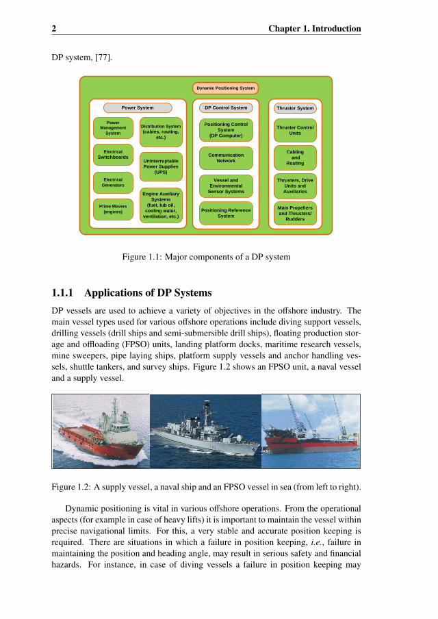
2 Chapter 1. Introduction
DP system, [77].
Positioning Control System
(DP Computer)
CommunicationNetwork
Vessel and Environmental
Sensor Systems
Positioning Reference System
DP Control System
Dynamic Positioning System
Main Propellers and Thrusters/
Rudders
Thrusters, Drive Units andAuxiliaries
Cablingand
Routing
Thruster ControlUnits
Thruster System
Distribution System(cables, routing,
etc.)
Uninterruptable Power Supplies
(UPS)
Engine Auxiliary Systems
(fuel, lub oil, cooling water,
ventilation, etc.)
Power System
Power Management
System
ElectricalSwitchboards
Electrical Generators
Prime Movers (engines)
Figure 1.1: Major components of a DP system
1.1.1 Applications of DP SystemsDP vessels are used to achieve a variety of objectives in the offshore industry. Themain vessel types used for various offshore operations include diving support vessels,drilling vessels (drill ships and semi-submersible drill ships), floating production stor-age and offloading (FPSO) units, landing platform docks, maritime research vessels,mine sweepers, pipe laying ships, platform supply vessels and anchor handling ves-sels, shuttle tankers, and survey ships. Figure 1.2 shows an FPSO unit, a naval vesseland a supply vessel.
Figure 1.2: A supply vessel, a naval ship and an FPSO vessel in sea (from left to right).
Dynamic positioning is vital in various offshore operations. From the operationalaspects (for example in case of heavy lifts) it is important to maintain the vessel withinprecise navigational limits. For this, a very stable and accurate position keeping isrequired. There are situations in which a failure in position keeping, i.e., failure inmaintaining the position and heading angle, may result in serious safety and financialhazards. For instance, in case of diving vessels a failure in position keeping may

1.1. What is a Dynamic Positioning (DP) System? 3
result in the death or injury of the divers. In situations where the operation is beingcarried out very close to a fixed structure, then a position keeping failure may resultin a collision. Consequently, damage to the structure or vessel, equipment, or a delayin the operation may occur. For instance, if a drilling vessel working in deep watersmakes widely twitchy movements then it will cause damage to riser pipes or drillingpipes and subsequently the drilling operation will be abrupted.
The position keeping failure may occur because of multiple reasons; technicalfailure of the DP equipment, operator’s error, extreme weather conditions not incor-porated in the control design strategy, etc. In many ships and various operations, theoveractuation feature is included to enhance the operational continuity by reducingthe chances of failure of the propulsion and measurement systems. This feature givesrise to the problem of optimal allocation because in the presence of this feature therecan be many possible combinations of actuators to yield a specific control action.
With the growing demand of the offshore industry, the development in the DPtechnologies is proliferating to meet the stringent safety, production and explorationdemands. This has made the users and the manufacturers of the DP systems strivehard towards more refinements in the DP related equipments and expertise. Conse-quently, there have been developments in all the faculties of the DP technologies likenavigation, control, propulsion and power units, and other subsidiary components.
DP systems have emerged as a popular replacement for the conventional positionkeeping techniques: anchoring and jack-up barge. While the conventional tools haveno or limited maneuverability, DP systems have excellent maneuverability and canbe easily moved from one place to another. No additional external equipment likethe anchoring tugs are required for DP systems. The anchoring may take severalhours but DP has very quick setup. The conventional techniques are limited by thesea obstructions and sea depth but DP systems do not have such limitations. Formore information on the design, principles, and applications of dynamic positioningsystems interested readers are referred to [23].
1.1.2 Focus of this Research
It is clear from the foregoing discussion that a DP system consists of several compo-nents. The focus of this thesis is the design and analysis of the positioning controlsystem of the vessel, a sub-component of the DP control system. This componentmay well be considered as the heart of the DP system as it interacts with the rest ofthe components of the DP system. There can be different control design objectivesdepending upon the nature and demands of a DP operation. Some of these control ob-jectives include position and heading regulation, path following, trajectory tracking,and wave-induced motion reduction. We focus on the position and heading regulation.
The basic element of a positioning control system is a mathematical model of thevessel which is an approximation of the reality. We consider a nonlinear vessel modelfrom [24] and this model serves as a prototype for this study. The model will be intro-duced in Chapter 2. We study the design and analysis of the control laws to stabilize(or regulate) the model to a desired equilibrium point. From a physical point of view,we desire to maintain the position and heading of the vessel within desired limits. Incontrol design, it is important to take into account the size and the dynamic response

4 Chapter 1. Introduction
of the thrust devices which must be adequate to cope with various environmental con-ditions in different offshore operations. In practice, the maximum thrust forces andmoments to maintain the position and heading in different environmental conditionsare estimated and then the capability of the thrust devices to meet the demands isanalyzed. This study is called a capability study.
The prototype vessel model is nonlinear due to the heading angle of the vessel.In [8], the state dependent coefficient (SDC) parametrization is introduced which is astrategy to transform the nonlinear system into a pseudo-linear form. The advantageof this approach is that it provides an opportunity to use concepts from linear systemtheory to study the nonlinear vessel model. We use the SDC framework throughoutthis thesis to study the control system design for the DP vessel.
The stability analysis is the an important feature of many control system designs.An unstable system may be potentially dangerous. Qualitatively, a dynamic system iscalled stable if starting from a position somewhere near its equilibrium or operatingpoint implies that it will stay around the point ever after. Due to complex and exoticbehavior of the nonlinear systems, more refined concepts of stability such as (local andglobal) asymptotic stability are required to describe the behavior of nonlinear systems.The asymptotic behavior implies that beside being stable, the system will converge toits equilibrium or operating position as time goes on.
Lyapunov stability theory is the most commonly used tool to study the stabilityproperties of nonlinear systems. The prototype vessel model has a typical nonlinearity,when described in pseudo-linear form by using the SDC parametrization. We beginour study with the stability analysis of pseudo-linear systems similar to the prototypeDP vessel system. The special form of the vessel model motivated us to combine theLyapunov stability theory with linear matrix inequalities (LMIs) to come up with anew method to analyze the global asymptotic stability of the pseudo-linear systems ofthe form similar to the prototype vessel model.
PID controllers are commonly used in practice. We use the SDC framework tocome up with the nonlinear version of the PID controller by using the state dependentalgebraic Riccati equation (from now on we call it the SDARE) technique for thedesign of a stabilizing control law for the DP vessel. The computation of the controllerand the observer gains require online computation of the solution of the SDARE. Itcan require large computation time, especially, for large systems. There are variousoff-the-shelf methods for the solution of the SDARE. We come up with a new method,the Fourier series interpolation (FSI) method, to solve the SDARE corresponding tothe DP vessel model. The FSI method reduces the computation time for the SDAREin comparison with the Schur decomposition method.
The port-Hamiltonian formulation has also become a popular technique to studyphysical systems since a decade. We transform the DP vessel model into port-Hamiltonianform and then use the IDA-PBC design approach to come up with a family of controllaws. These control laws may also be seen as the nonlinear version of the well-knownPID controllers, in the port-Hamiltonian framework.
1.2. An Overview of this Thesis 5
1.2 An Overview of this Thesis
Chapters 1 and 2 contain the basic introductory material about the main theme of thisthesis. Our focus in this thesis is to address the control system design problem fordynamic positioning of a sea vessel. The first chapter of this thesis introduces thedynamic positioning problem. The DP system is illustrated and the importance ofdynamic positioning is highlighted by describing its applications in various offshoreand onshore operations. The second chapter introduces the details of the mathematicalmodel we use in this thesis to describe the vessel motion. It highlights the necessarydetails of the vessel motion in mathematical form.
The main subject of the third chapter is the study of global asymptotic stability ofa special type of nonlinear systems which are similar to the prototype vessel model.The SDC framework is used to express the nonlinear system in a pseudo-linear formand then the stability is analyzed based on the properties of the state dependent systemmatrix. Two counterexamples are presented in this chapter. The first counterexampleshows that the conditions, that the system matrix in pseudo-linear form is continuous,Hurwitz, and exponentially bounded, as reported in the literature on this subject, arenot sufficient for global asymptotic stability of the pseudo-linear system. In the secondcounterexample, in addition to the set of conditions mentioned in the first counterex-ample, additionally, we also assume that the system matrix is periodic. It is shownthat the extended set too does not constitute the set of sufficient conditions for globalasymptotic stability of the pseudo-linear system. Apart from this, we also propose inthis chapter, a method for proving global asymptotic stability of the special pseudo-linear systems by combining the Lyapunov stability theory and the LMIs.
The fourth chapter addresses the control system design problem. The SDAREbased control design and estimation technique is used to design an SDARE controllerand an SDARE observer for dynamic positioning of the vessel. The fifth chapter isabout the FSI method for the approximation of the solution of the SDARE. The FSImethod reduces the online computations of the solution of the SDARE by performingthe computationally expensive tasks offline. The sixth chapter is also about the controlsystem design problem of the DP vessel. The main idea is to transform the vesselmodel in the port-Hamiltonian structure and then use the IDA-PBC design approach toaddress the control design problem. The thesis is concluded with the seventh chapterwhich briefly summarizes the thesis and provides some concluding remarks. Thehindsight ideas for future research are also presented in this chapter.
1.3 Contributions of this Thesis
We study the stability analysis of nonlinear systems in the SDC framework. Therehad been some existing results on this subject. Our main contribution on this topicare two counterexamples. It is claimed in the literature that it is sufficient for globalasymptotic stability of a pseudo-linear system that the system matrix in its SDC formis continuous, Hurwitz, and exponentially bounded. In a first counterexample, weshow that this claim is not valid. Motivated by the special type of state dependenceof the system matrix in DP vessel model, we assume additionally that the system
6 Chapter 1. Introduction
matrix is periodic and show by means of another counterexample that an additionalcondition also does not guarantee the stability of the nonlinear system. Each of thesecounterexamples have separately been published, see [58] and [59].
The special form of the nonlinearity in the vessel model and the Lyapunov stabilitytheory has lead us to propose a new approach to prove global asymptotic stability ofthe special type of pseudo-linear systems which resembles the prototype DP vesselmodel. This approach makes use of the LMIs to achieve global asymptotic stability.The approach is useful in particular for the vessel model and in general for the systemshaving similar structure as the vessel model.
Another contribution is the SDARE controller design for the DP vessel. The modelbased SDARE controller is a state feedback controller. The complete state of the DPvessel model is not available in practice. Therefore, a state observer is also required.We also used the SDARE observer to find the state estimate. It has been shown that theSDARE controller in combination with the SDARE observer gives the desired stabilityand performance of the DP vessel. Alongside the SDARE controller and observer, anumerical method for the approximation of the solution of the SDARE is proposed.We call this the Fourier series interpolation (FSI) method. This method is proved tobe very handy in reducing the online computation time of the SDARE for controllerand observer gains computations. The concept of the FSI method has been presentedin a conference paper, see [57].
The final contribution of this thesis is the use of the port-Hamiltonian structureand the passivity theory for the first time for DP vessel control design. We propose afamily of passivity based controllers for the DP vessel. Passivity idea is very attractivein a sense that it helps in assigning the physical meaning to various variables andquantities. The stability and performance of the family of the IDA-PBC designs arediscussed. This idea was presented at a conference (see [55]) and it has recently beenaccepted in a journal (see [56]).
Chapter 2Mathematical Model of a SeaVessel
The details of a vessel model for DP considerations are presented in this chapter.The prototype vessel model described in this chapter will be used in the subse-
quent chapters for studying the control system design of the DP vessel.
2.1 Motion of a floating VesselIn this section, we explain various terms associated with the motion of the vessel inthe sea. Motion of a floating vessel can be described by six degrees of freedom (DOF),i.e., a vessel can move in six different directions. We can categorize the six DOF intwo categories:
1. The translational motion in the following three directions,
• Surge: motion in backward (aft/stern) and forward (bow/fore) directions
• Sway: motion along sideways (transversial directions): starboard (right side ofthe ship) and port (left side of the ship) directions
• Heave: motion in upward and downward directions
2. The rotational motion in the following three directions,
• Roll: rotation about the surge axis
• Pitch: rotation about the sway axis
• Yaw: rotation about the heave axis
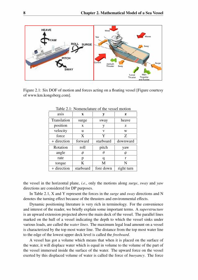
Various modes of motion and the forces acting on the vessel are shown in Figure 2.1and summarized in Table 2.1. A DP system is concerned primarily with control of
7
8 Chapter 2. Mathematical Model of a Sea Vessel
HEAVE
YAW
SWAY
PITCH
SURGEROLL
Figure 2.1: Six DOF of motion and forces acting on a floating vessel [Figure courtesyof www.km.kongsberg.com].
Table 2.1: Nomenclature of the vessel motionaxis x y z
Translation surge sway heaveposition x y zvelocity u v w
force X Y Z+ direction forward starboard downward
Rotation roll pitch yawangle φ θ ψ
rate p q rtorque K M N
+ direction starboard fore down right turn
the vessel in the horizontal plane, i.e., only the motions along surge, sway and yawdirections are considered for DP purposes.
In Table 2.1, X and Y represent the forces in the surge and sway directions and Ndenotes the turning effect because of the thrusters and environmental effects.
Dynamic positioning literature is very rich in terminology. For the convenienceand interest of the reader, we briefly explain some important terms. A superstructureis an upward extension projected above the main deck of the vessel. The parallel linesmarked on the hull of a vessel indicating the depth to which the vessel sinks undervarious loads, are called the water lines. The maximum legal load amount on a vesselis characterized by the top most water line. The distance from the top most water lineto the edge of the lowest upper deck level is called the freeboard.
A vessel has got a volume which means that when it is placed on the surface ofthe water, it will displace water which is equal in volume to the volume of the part ofthe vessel immersed inside the surface of the water. The upward force on the vesselexerted by this displaced volume of water is called the force of buoyancy. The force

2.2. Mathematical Model Describing the Dynamics of a floating Vessel 9
of buoyancy depends on characteristics of water: it is low for fresh and warm waterand it is high for cold and saline water which has more density. The center of massof the water displaced by the vessel is called the center of buoyancy. The point atwhich the weight of the vessel is considered to act is called the center of gravity. Thepoint of intersection of the vertical lines through the center of gravity and the centerof buoyancy is called the metacenter.
The rear or aft part of the vessel is called the stern. Usually, during the night time,the stern of the vessel is indicated with a white navigation light on it. The foremostpart of the vessel, opposite to the stern part, when the vessel is underway, is called thebow. The right hand side of the vessel as perceived by a person on board facing thebow is called the starboard. The opposite part of the vessel on the left hand side willthen be called the port. All these terms are linked with the main deck of the vesseland has nothing to do with the location of the superstructure on the deck. Figure 2.2illustrates all these terms.
Super Structure
Water line
Free board
Aft or Stern
Fore or Bow
Star-board side
Port side
Figure 2.2: Commonly used terms in literature on dynamic positioning
2.2 Mathematical Model Describing the Dynamics of afloating Vessel
Modern DP control systems for ships use controllers based on a mathematical modelof the ship. This mathematical model describes the hydrodynamic, damping, environ-
10 Chapter 2. Mathematical Model of a Sea Vessel
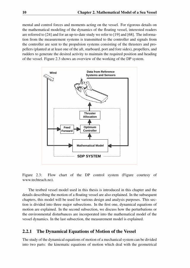
mental and control forces and moments acting on the vessel. For rigorous details onthe mathematical modeling of the dynamics of the floating vessel, interested readersare referred to [24] and for an up-to-date study we refer to [19] and [68]. The informa-tion from the measurement systems is transmitted to the controller and signals fromthe controller are sent to the propulsion systems consisting of the thrusters and pro-pellers (planted at at least one of the aft, starboard, port and fore sides), propellers, andrudders to generate the desired activity to maintain the required position and headingof the vessel. Figure 2.3 shows an overview of the working of the DP system.
Optimum
Controller
Thruster
Allocation
Mathematical Model
SDP SYSTEM
Data from Reference
Systems and Sensors
Feed
Forward
Wind
Figure 2.3: Flow chart of the DP control system (Figure courtesy ofwww.techteach.no).
The testbed vessel model used in this thesis is introduced in this chapter and thedetails describing the motion of a floating vessel are also explained. In the subsequentchapters, this model will be used for various design and analysis purposes. This sec-tion is divided into three major subsections. In the first one, dynamical equations ofmotion are explained. In the second subsection, we discuss how the perturbations orthe environmental disturbances are incorporated into the mathematical model of thevessel dynamics. In the last subsection, the measurement model is explained.
2.2.1 The Dynamical Equations of Motion of the Vessel
The study of the dynamical equations of motion of a mechanical system can be dividedinto two parts: the kinematic equations of motion which deal with the geometrical
2.2. Mathematical Model Describing the Dynamics of a floating Vessel 11
aspects of the equations of motion, and the kinetic equations of motion which dealwith the analysis of the forces causing the motion.
The Kinematic Equations of Motion
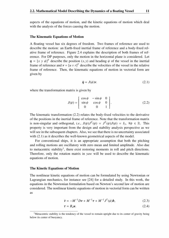
A floating vessel has six degrees of freedom. Two frames of reference are used todescribe the motion: an Earth-fixed inertial frame of reference and a body-fixed rel-ative frame of reference. Figure 2.4 explains the description of both frames of ref-erence. For DP purposes, only the motion in the horizontal plane is considered. Letη = [x y ψ]T describe the position (x, y) and heading ψ of the vessel in the inertialframe of reference and ν = [u v r]T describe the velocities of the vessel in the relativeframe of reference. Then, the kinematic equations of motion in vectorial form aregiven by
η = J(ψ)ν. (2.1)
where the transformation matrix is given by
J(ψ) =
cosψ − sinψ 0sinψ cosψ 0
0 0 1
. (2.2)
The kinematic transformation (2.2) relates the body-fixed velocities to the derivativeof the positions in the inertial frame of reference. Note that the transformation matrixis non-singular and orthogonal, i.e., J(ψ)JT (ψ) = JT (ψ)J(ψ) = I3, ∀ψ ∈ R. Thisproperty is very important from the design and stability analysis perspective as wewill see in the subsequent chapters. Also, we see that there is no uncertainty associatedwith (2.1) as it describes the well-known geometrical aspects of the model.
For conventional ships, it is an appropriate assumption that both the pitchingand rolling motions are oscillatory with zero mean and limited amplitude. Also dueto metacentric stability1, there exist restoring moments in roll and pitch directions.Therefore, only the rotation matrix in yaw will be used to describe the kinematicequations of motion.
The Kinetic Equations of Motion
The nonlinear kinetic equations of motion can be formulated by using Newtonian orLagrangian mechanics, for instance see [24] for a detailed study. In this work, theequations in the Newtonian formulation based on Newton’s second law of motion areconsidered. The nonlinear kinetic equations of motion in vectorial form can be writtenas
ν = −M−1Dν + M−1τ + M−1JT (ψ)b, (2.3)
τ = Buu. (2.4)
1Metacentric stability is the tendency of the vessel to remain upright due to its center of gravity beingbelow its center of buoyancy.

12 Chapter 2. Mathematical Model of a Sea Vessel
rO
rXrY
Y
XO
Figure 2.4: The Earth-fixed and the vessel-fixed frames of reference.
In (2.3) and (2.4), the vector τ = [X,Y,N]T ∈ R3×1 represents the control forcesand moment acting on the vessel in the body-fixed frame of reference, provided bythe propulsion system of the ship consisting of propellers and thrusters. The vectoru ∈ Rr×1 (r ≥ 1) describes the control inputs and the matrix Bu ∈ R
3×r is a constantmatrix describing the actuator configurations. The vector u is the command to theactuators, which are assumed to have much faster dynamic response than the vessel;thus the coefficient Bu represents the mapping from the actuator command to the forcegenerated by the actuators. In the following chapters, we assume a fully actuatedvessel model and we will take Bu = I3. In the forthcoming chapters, we therefore usethe vectors τ and u interchangeably, unless it is specified. The matrices M and D are3 × 3 inertia and damping matrices, respectively. The vector b ∈ R3×1 represents theslowly varying bias forces and moments in the Earth-fixed inertial frame of reference,due to the waves, wind, sea currents, and other environmental factors surrounding thevessel.
For DP consideration, the inertia matrix has the following form
M =
m − Xu 0 00 m − Yv mxG − Yr
0 mxG − Nv Iz − Nr
∈ R3×3, (2.5)
where m is the vessel mass, Iz is the moment of inertia about the vessel-fixed z-axis,and xG denotes the longitudinal position of the center of gravity of the vessel withrespect to the relative frame of reference. The added masses due to acceleration in thesurge, sway, and yaw directions are defined as
XuM=∂X∂u, Yv
M=∂Y∂v, Nr
M=∂N∂r, Yr
M=∂Y∂r, Nv
M=∂N∂v. (2.6)

2.2. Mathematical Model Describing the Dynamics of a floating Vessel 13
Note that the inertia along the surge direction is decoupled from the inertia effectsalong the sway and yaw directions. Due to small velocities and starboard-port sym-metries of the vessel, the added mass in sway due to the angular acceleration in yawis equal to the added mass in yaw due to sway acceleration, i.e., Yr = Nv. Hence,in DP applications, it is assumed that the matrix M is symmetric and strictly positivedefinite, i.e., M = MT > 0. This assumption is very useful for the purpose of analysis.
The vessel motion generates waves. This means energy is transferred from vesselto the fluid and this energy is modeled by the linear damping term. The linear dampingmatrix D for DP is taken as
D =
−Xu 0 00 −Yv −Yr
0 −Nv −Nr
∈ R3×3. (2.7)
In most DP applications, the damping matrix is assumed to be real, non-symmetrical,and positive definite. However, for low speed applications where the damping matrixis reduced to (2.7), it can be assumed that Nv = Yr. In such a case, we assume thedamping matrix D to be real, symmetric, and positive definite. The damping compo-nents in surge, sway, and yaw directions are defined by
XuM=∂X∂u, Yv
M=∂Y∂v, Nr
M=∂N∂r, Yr
M=∂Y∂r, Nv
M=∂N∂v. (2.8)
Decoupling of the surge mode from the sway and yaw modes is beneficial for theconvergence of parameter estimation algorithms, see [28]. An a priori estimate of themass and damping parameters of the vessel can be obtained by using semi-empiricalmethods and hydrodynamic computations. See [22] for details about the identificationand estimation of vessel model parameters. Often the estimates of mass and dampingparameters are updated based on the data obtained from the practical experiments incalm waters.
2.2.2 The Disturbances Model
The forces acting on a sea vessel can be categorized in two main categories [37]: theinternal and the external forces and moments. The internal forces and moments areformulated as functions of acceleration, velocities, propeller propulsions, and rudderexcitations. These have partially been discussed in the previous subsection. Herewe explain the external forces acting on the vessel. These forces are also termed asexternal disturbances. The external disturbances can be distinguished into 3 majorcategories [83]:
• Additive disturbances - These are the disturbances due to wind, waves, sea cur-rents, etc. These forces act additively on the vessel. To model and analyze theseforces, the model of the ship is extended by adding additional states.
• Multiplicative disturbances - A vessel in sea is also subject to the time varyingparameters such as load conditions, water depth, trim, speed changes, etc. Thesedisturbances are called multiplicative disturbances.
14 Chapter 2. Mathematical Model of a Sea Vessel
• Measurement disturbances - These are the disturbances due to the wrong func-tioning or noise in the measurement devices like DGPS and gyro compass.
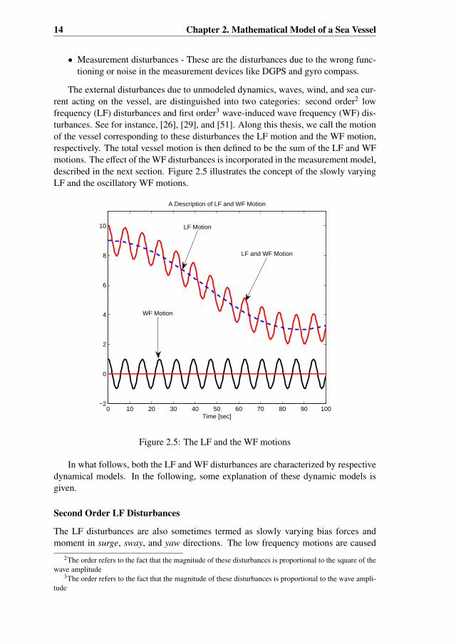
The external disturbances due to unmodeled dynamics, waves, wind, and sea cur-rent acting on the vessel, are distinguished into two categories: second order2 lowfrequency (LF) disturbances and first order3 wave-induced wave frequency (WF) dis-turbances. See for instance, [26], [29], and [51]. Along this thesis, we call the motionof the vessel corresponding to these disturbances the LF motion and the WF motion,respectively. The total vessel motion is then defined to be the sum of the LF and WFmotions. The effect of the WF disturbances is incorporated in the measurement model,described in the next section. Figure 2.5 illustrates the concept of the slowly varyingLF and the oscillatory WF motions.
0 10 20 30 40 50 60 70 80 90 100−2
0
2
4
6
8
10
Time [sec]
A Description of LF and WF Motion
WF Motion
LF Motion
LF and WF Motion
Figure 2.5: The LF and the WF motions
In what follows, both the LF and WF disturbances are characterized by respectivedynamical models. In the following, some explanation of these dynamic models isgiven.
Second Order LF Disturbances
The LF disturbances are also sometimes termed as slowly varying bias forces andmoment in surge, sway, and yaw directions. The low frequency motions are caused
2The order refers to the fact that the magnitude of these disturbances is proportional to the square of thewave amplitude
3The order refers to the fact that the magnitude of these disturbances is proportional to the wave ampli-tude

2.2. Mathematical Model Describing the Dynamics of a floating Vessel 15
by the forces generated by the thrusters and propellers, wind forces, wave-inducedforces, and hydrodynamic forces. In marine control applications, these forces andmoment can be described, [24], by the first order Markov process given by
b = −T−1b + Ψwb, (2.9)
where b ∈ R3×1 is a vector of bias forces and moment, the vector wb ∈ R3×1 represents
the zero-mean Gaussian white noise process, i.e., wb ∼ N(0,Qc,b), T ∈ R3×3 is adiagonal matrix of positive bias time constants and Ψ ∈ R3×3 is a diagonal matrixscaling the amplitude of the noise vector wb. The matrix T is known as the timeconstant. In this context it will have relatively large values as sea states change veryslowly. We can also interpret (2.9) as a low-pass filter.
In many applications, see for instance [27, 80], it is considered more appropriatefrom a physical point of view to use b = Ψwb to describe the bias model. Thismay be described as integration of the noise signal which in fact is a random walkphenomenon. Thus bias forces and moments are sometimes modeled as a randomwalk process. Another case could be that the bias forces and moment are constant.Then the bias model will be b = 0.
First Order Wave-Induced WF Disturbances
The fundamental assumption for the development of the WF motion model is that thesea state is known and can be described by a spectral density function. The first orderwave-induced WF disturbances in surge, sway, and yaw directions are modeled assecond order harmonic oscillations which are driven by Gaussian white noise process.It was Balchen who first modeled the WF motion in this way, [6]. For each of thethree directions, the WF disturbances model in the frequency domain is given by
ξi(s) =σis
s2 + 2ζiω0is + ω20i
wξi(s), i = 1, 2, 3 (2.10)
where ω0i is the dominating (sometimes also termed as undamped) wave frequency,ζi is the relative damping ratio, and σi is the wave intensity parameter. The input wξi
represents the Gaussian white noise process, i.e., wξi ∼ N(0,Qc,ξi). The damping ratioζi is a measure to describe how the oscillations in the system (2.10) decay when adisturbance is introduced. Normally, the damping ratio defines the level of damping(under-damped, over-damped, critically-damped, and undamped) of the system. Thedominating wave frequency ω0i is obtained by spectral analysis.
In state space representation, the WF disturbances model for each direction can bewritten as
ξ(i)1 = ξ(i)
2
ξ(i)2 = −ω2
0iξ(i)1 − 2ζiω0iξ
(i)2 + σiwi, i = 1, 2, 3 (2.11)
A compact state space realization of the WF model is given by[ξ1
ξ2
]=
[O3 I3
−Ω2 −2ZΩ
] [ξ1
ξ2
]+
[O3
Σ
]wξ, (2.12)
16 Chapter 2. Mathematical Model of a Sea Vessel
where ξ1 = [ξ(1)1 , ξ(2)
1 , ξ(3)1 ]T , ξ2 = [ξ(1)
2 , ξ(2)2 , ξ(3)
2 ]T , Ω = diagω01, ω02, ω03, Z =
diagζ1, ζ2, ζ3, and Σ = diagσ1, σ2, σ3. The matrix O3 ∈ R3×3 is a zero matrix.
The WF motion parameters ω0, ζ, and σ depend on the sea states, structure of thevessel and the direction of the incident waves. The vector wξ describes the Gaussianwhite noise process, i.e., wξ ∼ N(0,Qc,ξ) The state vector may or may not have aphysical interpretation depending on the particular state-space realization used.
For DP operations only the LF motion is required to be controlled. This is im-portant to avoid unnecessary power consumption and possible wear and tear of theactuators. Therefore, the oscillatory WF motion is required to be filtered or separatedfrom the LF motion. The WF response is required to be controlled in certain oper-ations like ride control of a passenger vessel, where reducing pitch and role motionhelps avoiding motion sickness. The stochastic nature of environmentally inducedforces and moments has made the Kalman filter an essential part of the modern seavessel motion control systems.
Filtering of the WF motion can be done either by using appropriate classical fil-tering techniques or it can be done by state estimation. Using filtering techniques, itis important to know the threshold frequency. Another problem with the filtering ap-proach is possible phase lag due to delay of the signals. For an estimation approach,we need to know the parameters of the system. Even in the linearized case, parametersare required. It is also important to keep in mind that the linearized model may not bea good approximation of the actual model or system.
2.2.3 The Measurement ModelThe position and heading of the vessel in the inertial frame of reference can be mea-sured by using a differential global positioning system (DGPS) and a gyro-compass.For reliability, some vessels have multiple sensors. The measurement model can bedescribed, using the superposition principle, by the following vector equation
y = yb + yξ + υ, (2.13)
where yb = η and yξ = ξ1 are, respectively, the position and heading measurementsof the vessel corresponding to the LF and the WF motions and the vector v ∈ R3×1
is the Gaussian white noise process, i.e., υ ∼ N(0,Rc). The vector v describes themeasurement noise.
2.2.4 Wave FilteringIn (2.13), the measured output is assumed to essentially contain the LF and WF mo-tion components. The separation of the WF component from the LF component istermed as wave filtering. This action is also important to avoid thruster modulation, aphenomenon which gives rise to high frequency fluctuations in the thrust demand inthe control loop. Knowledge of the sea states is required to determine the WF mo-tion of the vessel. Sea states can be distinguished in 9 different forms (calm, smooth,rough, high, phenomenal, etc.) depending on the significant wave height [24].
Low-pass, notch, and deadband filters were the most commonly used wave filter-ing techniques in earlier DP systems, for instance see [82]. The main drawback of
2.3. Summary of the Mathematical Model 17
these techniques was the problem to meet the high gain control requirements due to asignificant phase lag. In earlier DP systems, wave filtering was accomplished by us-ing a proportional controller with a deadband non-linearity. This deadband produced anull control action until the control signal was inside the deadband. The length of thisdeadband could be increased by the operator with changing weather conditions. Thischange in length was termed as ‘weather’ as it was subject to the weather conditions[82].
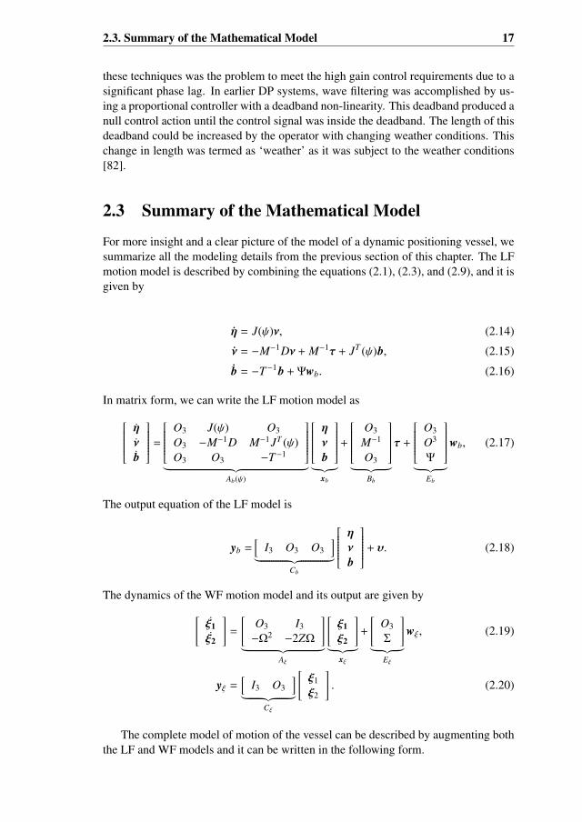
2.3 Summary of the Mathematical Model
For more insight and a clear picture of the model of a dynamic positioning vessel, wesummarize all the modeling details from the previous section of this chapter. The LFmotion model is described by combining the equations (2.1), (2.3), and (2.9), and it isgiven by
η = J(ψ)ν, (2.14)
ν = −M−1Dν + M−1τ + JT (ψ)b, (2.15)
b = −T−1b + Ψwb. (2.16)
In matrix form, we can write the LF motion model as ηνb =
O3 J(ψ) O3
O3 −M−1D M−1JT (ψ)O3 O3 −T−1
︸ ︷︷ ︸Ab(ψ)
ηνb︸︷︷︸
xb
+
O3
M−1
O3
︸ ︷︷ ︸Bb
τ +
O3
O3
Ψ
︸ ︷︷ ︸Eb
wb, (2.17)
The output equation of the LF model is
yb =[
I3 O3 O3
]︸ ︷︷ ︸Cb
ηνb + υ. (2.18)
The dynamics of the WF motion model and its output are given by[ξ1ξ2
]=
[O3 I3
−Ω2 −2ZΩ
]︸ ︷︷ ︸
Aξ
[ξ1ξ2
]︸ ︷︷ ︸
xξ
+
[O3
Σ
]︸ ︷︷ ︸
Eξ
wξ, (2.19)
yξ =[
I3 O3
]︸ ︷︷ ︸Cξ
[ξ1
ξ2
]. (2.20)
The complete model of motion of the vessel can be described by augmenting boththe LF and WF models and it can be written in the following form.

18 Chapter 2. Mathematical Model of a Sea Vessel
ηνbξ1ξ2
=
O3 J(ψ) O3 O3 O3O3 −M−1D M−1 JT (ψ) O3 O3O3 O3 −T−1 O3 O3O3 O3 O3 O3 I3O3 O3 O3 −Ω2 −2ZΩ
︸ ︷︷ ︸A(ψ)
ηνbξ1ξ2
︸ ︷︷ ︸x
+
O3
M−1
O3O3O3
︸ ︷︷ ︸B
τ +
O3 O3O3 O3Ψ O3O3 O3O3 Σ
︸ ︷︷ ︸E
[wbwξ
]︸ ︷︷ ︸
w
.
(2.21)
The output of (2.21) can be obtained by using the superposition principle, see (2.13),and is written in matrix form as
y =[
I3 O3 O3 I3 O3
]︸ ︷︷ ︸C
ηνbξ1
ξ2
+ υ. (2.22)
The complete model of the vessel in compact form is written as
x =A(ψ)x + Bτ + Ew, (2.23)
y =Cx + υ. (2.24)
The vectors w and v represent the Gaussian white noise processes, i.e., w ∼ N(0,Qc)and υ ∼ N(0,Rc), where Qc = diagQc,b,Qc,ξ. The system (2.23)-(2.24) is a pseudo-linear system because of dependency of the system matrix A(ψ) on the heading angle.We call this pseudo-linear form the state dependent coefficient (SDC) parametrizationof nonlinear system. Chapter 3 explains the concept of the SDC parametrization inmore detail.
2.4 Properties of the ModelIn this thesis, we deal with the control design and estimation problems of the DP vesseldiscussed in the previous sections. For this purpose, it is important to know certainproperties of the vessel model which play a fundamental part in the control design andestimation techniques which we are going to use in the subsequent chapters. Theseproperties include controllability, observability, stabilizability, and detectability. Inthe following, we recall some important results about these properties in the contextof the pseudo-linear systems, presented in [7] .
Definition 2.4.1. (Controllability in terms of rank condition) The pseudo-linearsystem of the form (2.23)-(2.24) with an n-dimensional state vector is pointwise con-trollable iff the rank of the controllability matrix
C =[
B A(ψ)B A2(ψ)B · · · An−1(ψ)B], (2.25)
is n, for each ψ ∈ R. In other words, we also say the pair (A(ψ), B) is pointwisecontrollable.

2.4. Properties of the Model 19
Definition 2.4.2. (Observability in terms of rank condition) The pseudo-linear sys-tem of the form (2.23)-(2.24) with an n-dimensional state vector is pointwise observ-able iff the rank of the observability matrix
O =
CCA(ψ)CA2(ψ)
...
CAn−1(ψ)
, (2.26)
is n, for each ψ ∈ R. In other words, we also say the pair (C, A(ψ)) is pointwiseobservable.
It can easily be checked that the controllability matrices corresponding to the sys-tems (2.17) and (2.21) have rank 6 for all ψ ∈ R, i.e., only the position and the veloci-ties can be controlled. This is not restrictive as the LF bias forces and the WF motionscannot be controlled. The observability matrices corresponding to both the systemshave full column ranks for all ψ ∈ R. So the systems are pointwise observable, i.e.,we can build the states of the system from the knowledge of the input and the output.
The stabilizability and detectability are weaker conditions than the controllabilityand observability, respectively. These properties are important from the point of viewof the existence of the solution of the SDARE. In the following, we define a necessaryand sufficient condition for the pointwise stabilizability and detectability of a pseudo-linear system, see [7] for more details.
Definition 2.4.3. (Pointwise Stabilizability) The pseudo-linear system of the form of(2.23)-(2.24) with an n-dimensional state vector is pointwise stabilizable iff
rank(λI − A(ψ) B
)= n, (2.27)
for each eigenvalue λ of A(ψ) which has a non-negative real part (Re(λ ≥ 0)) and forall ψ ∈ R. In other words, we also say the pair (A(ψ), B) is stabilizable.
Definition 2.4.4. (Pointwise Detectability) The pseudo-linear system of the form(2.23)-(2.24) with an n-dimensional state vector is pointwise detectable iff
rank(λI − A(ψ)
C
)= n, (2.28)
for each eigenvalue λ of A(ψ) which has a non-negative real part (Re(λ ≥ 0)) and forall ψ ∈ R. In other words, we also say the pair (C, A(ψ)) is detectable.
Due to the special structure of the system matrices Ab(ψ) in (2.17) and A(ψ) in(2.21), the eigenvalues of the system matrices do not change with the variable ψ. Theonly non-negative eigenvalue of both Ab(ψ) and A(ψ) is 0 with algebraic multiplicity3. This makes it an easy task to compute the rank conditions (2.27) and (2.28). Itcan be checked that the rank is 9 for both stabilizability and detectability conditionscorresponding to Ab(ψ) and it is 15 for A(ψ). Thus both the systems (2.17) and (2.21)are pointwise stabilizable and detectable.

20
Chapter 3SDC Parametrization andStability Analysis of AutonomousNonlinear Systems1
The stability analysis of nonlinear systems has always been a challenging task. Thisis mainly because of phenomena like finite escape time and limit cycles, see for
instance [32], [59], [79], [81], and [88]. Numerous techniques for stability analysis ofnonlinear systems have been proposed over time, for further details see [43], [45], and[86]. One such approach is to first write the nonlinear system dynamics in linear-likeform using a state dependent coefficient (SDC) parametrization and then analyze thepossible extension of the results of linear systems theory for the stability analysis ofnonlinear systems. The SDC representation provides a systematic way to analyze theextension of the results of linear systems theory for the stability analysis of nonlinearsystems.
3.1 State Dependent Coefficient ParametrizationLet Ω ⊆ Rn and f (x) be a vector function from Ω to Rn. Consider the followingnonlinear system
x = f (x), x0 = x(t0), (3.1)
where x ∈ Ω is the state of the system. If the vector function f : Ω −→ Rn, iscontinuously differentiable and f (0) = 02, then it is always possible to write f (x) =
A(x)x, see [46]. Let us call the matrix A(x) the state dependent coefficient (SDC)
1Section 3.4.1 and Section 3.5.1 of this chapter have been published in the form of two separate articlesin the IMA Journal of Mathematical Control and Information, see [58] and [59].
2When it is clear from context (by the domain and codomain of the function) we write, e.g., f (0) = 0for f (0) = 0, and A(0) for A(0)
21

22 Chapter 3. SDC Parametrization and Stability Analysis
parametrization of f (x). It is important to mention that the SDC parametrization isnot unique unless f (x) is a scalar function. For example, if A1(x) and A2(x) are twodistinct parametrizations of f (x) then for 0 ≤ α ≤ 1,
αA1(x)x + (1 − α)A2(x)x = α f (x) + (1 − α) f (x) = f (x),
i.e.αA1(x) + (1 − α)A2(x)
is also a parametrization of f (x). In fact infinitely many parametrizations are possiblebut one has to chose only those which are appropriate for the desired objectives. Formore details on the SDC parametrization, interested readers are referred to [36] and tothe references therein.
An important property of the SDC parametrization is that it preserves the lineariza-tion of nonlinear systems. If A(x) is any parametrization of f (x) then A(0) = 5 f |x=0.The following Lemma from [7] establishes this fact.
Lemma 3.1.1. For any SDC parametrization A(x) of f (x) with f (x) continuouslydifferentiable and f (0) = 0, A(0)x is the linearization of f (x) at the zero equilibrium.
Proof. See [7].
From here onward, we will use the notions of the coefficient matrix A(x) andthe system matrix interchangeably. Consider the following pseudo-linear autonomoussystem
x = A(x)x, x0 = x(t0). (3.2)
In the remainder of this chapter, we analyze the stability properties of the pseudo-linear system (3.2). Our approach is based on the properties of the system matrix A(x)in (3.2). In the following, we state four conditions on this matrix. To analyze thestability properties of (3.2), we will test all these conditions in the order in which theyare stated.
C.1 The matrix function, A : Ω −→ Rn×n is a C1 function3
C.2 A(x) is pointwise asymptotically stable (Hurwitz) matrix, i.e., all eigenvalues ofA(x) lie in the open left half plane for all x ∈ Ω. Consequently, we see that theorigin x = 0 is the only equilibrium point of the system (3.2).
C.3 The system matrix, A(x), is exponentially bounded i.e., ||eA(x)t || ≤ M for somereal M > 0 and ∀x ∈ Ω, ∀t ∈ [0,∞).
C.4 A(x) is a periodic function with a period θ, i.e., A(x + θ) = A(x), ∀ x ∈ Ω.
In Chapter 2, we have introduced a mathematical model of a vessel. The systemmatrix of this model is a periodic function of the heading angle of the vessel. This factis the motivation behind the fourth condition (C.4). The first two conditions imply that
3C1(Ω ⊆ Rn,Rn×m) := A : Ω −→ Rn×m | A is continuous, ∂xi A exists and are continuous for alli = 1, 2, ..., n.

3.2. Local Asymptotic Stability Analysis 23
there is only one isolated equilibrium point, x = 0, of (3.2). Therefore, the stabilityanalysis of (3.2) will be with reference to this equilibrium point. The conditions C.1and C.2 are sufficient to prove local asymptotic stability. The conditions C.3 and C.4are imposed to analyze global asymptotic stability.
3.2 Local Asymptotic Stability Analysis
We start with the local asymptotic stability considerations. It can be defined as follows[73]:
Definition 3.2.1. An equilibrium point x of the nonlinear system (3.2) is (locally)asymptotically stable if it is stable, and if in addition there exists some r > 0 such that||x(0)|| < r implies that x(t)→ x as t → ∞.
Since A(x) is continuously differentiable, therefore, colA(x) ∈ C1. By colA(x),we mean the set of columns of A(x). Applying the Mean Value Theorem [54] tocolA(x), we can write
col jA(x) = col jA(0) +∂col jA(z j)
∂xx, j = 1, 2, ..., n (3.3)
where the vector z j is a point, on the line connecting the origin and the point x, whichyields equality in the jth equation of (3.3). By col jA(x), we mean the jth column ofA(x). Using (3.3) in (3.2), we can write
x = A(0)x +[
∂col1A(z1)∂x x ∂col2A(z2)
∂x x ... ∂colnA(zn)∂x x
]x,
= A(0)x +
n∑j=1
n∑i=1
xix j∂col jA(z j)
∂xi.
Multiplying and dividing the second term by ||x|| and defining
ψ(x, z1, z2, ..., zn) M=n∑
j=1
n∑i=1
xix j
||x||∂col jA(z j)
∂xi,
we get,
x = A(0)x + ψ(x, z1, z2, ..., zn)||x||. (3.4)
Since
lim||x||→0
ψ(x, z1, z2, ..., zn) = 0, (3.5)
and A(0) is Hurwitz, x is a locally asymptotically stable equilibrium point of (3.4).This means, that the conditions C.1 and C.2 ensure that x is a locally asymptoticallystable equilibrium point of (3.2).
24 Chapter 3. SDC Parametrization and Stability Analysis
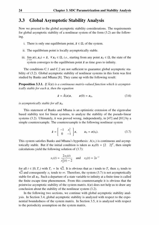
3.3 Global Asymptotic Stability AnalysisNow we proceed to the global asymptotic stability considerations. The requirementsfor global asymptotic stability of a nonlinear system of the form (3.2) are the follow-ing.
i. There is only one equilibrium point, x ∈ Ω, of the system.
ii. The equilibrium point is locally asymptotically stable.
iii. limt→∞
x(t, x0) = x, ∀ x0 ∈ Ω, i.e., starting from any point x0 ∈ Ω, the state of thesystem converges to the equilibrium point x as time goes to infinity.
The conditions C.1 and C.2 are not sufficient to guarantee global asymptotic sta-bility of (3.2). Global asymptotic stability of nonlinear systems in this form was firststudied by Banks and Mhana [8]. They came up with the following result:
Proposition 3.3.1. If A(x) is a continuous matrix-valued function which is asymptot-ically stable for each x, then the equation
x = A(x)x, x(0) = x0, (3.6)
is asymptotically stable for all x0.
This statement of Banks and Mhana is an optimistic extension of the eigenvaluebased stability test for linear systems, to analyze the stability of the pseudo-linearsystems (3.2). Ultimately, it was proved wrong, independently, in [47] and [81] by asimple counterexample. The counterexample is the following nonlinear system
x =
[−1 x2
10 −1
]x, x0 = x(t0). (3.7)
This system satisfies Banks and Mhana’s hypothesis: A(x1) is continuous and asymp-totically stable. But if the initial condition is taken as x0(0) = [2 2]T , then simplecalculations yield the following solution of (3.7):
x1(t) =2x2(t)
x22(t) − 2
and x2(t) = 2e−t
for all t ∈ [0,Tc) with Tc = ln√
2. It is obvious that as t tends to Tc then x2 tends to√2 and consequently x1 tends to∞. Therefore, the system (3.7) is not asymptotically
stable for all x0. Such a departure of a state variable to infinity at a finite time is calledthe finite escape time phenomenon. From this counterexample it is obvious that thepointwise asymptotic stability of the system matrix A(x) does not help us to draw anyconclusion about the stability of the nonlinear system (3.2).
In the following two sections, we continue with global asymptotic stability anal-ysis. In Section 3.4, global asymptotic stability is analyzed with respect to the expo-nential boundedness of the system matrix. In Section 3.5, it is analyzed with respectto the periodicity assumption on the system matrix.

3.4. Exponential Boundedness and Global Asymptotic Stability 25
3.4 Exponential Boundedness and Global AsymptoticStability
In this section, we continue with the findings of Langson and Alleyne and ultimatelygive a counterexample to show that global asymptotic stability is not guaranteed whenthe system matrix is exponentially bounded. Langson and Alleyne [47] studied thistopic further and concluded the following:
Proposition 3.4.1. Consider the system x = A(x)x, where A : Rn −→ Rn×n is uni-formly continuous in x and A(x) is a stable matrix ∀x ∈ Rn. The origin of the givensystem is an asymptotically stable equilibrium point.
Corollary 3.4.1. If the hypothesis of Proposition 3.4.1 is satisfied with ||eA(x)t || ≤
M for some real M > 0 and ∀x ∈ Rn, ∀t ∈ [0,∞), then the system x = A(x)x isasymptotically stable for any arbitrary finite initial condition.
In the following subsection, a counterexample [58] to these statements is pre-sented. We construct a system where the hypotheses of Langson and Alleyne men-tioned in Proposition 3.4.1 and Corollary 3.4.1 are satisfied, that is nonetheless notglobally asymptotically stable.
3.4.1 A Counterexample Showing that the Exponential Bounded-ness of the System Matrix does not Guarantee Global Asymp-totic Stability
Example 3.4.1. We start with the following SDC formulation of a nonlinear systemin a general setting
x =
[a b − c(x)
−b − c(x) a
]x, x0 = x(t0), (3.8)
where a, b ∈ R and c(x) is a smooth function: c : R2 → R. We show that the coefficientmatrix in (3.8) satisfies the hypothesis of Langson and Alleyne, for certain choices ofthe parameters a and b, and the scalar function c(x): a < 0 and b > |c(x)| for allx ∈ R2.
1. Continuity: From the description of the coefficient matrix in (3.8), it is obvi-ous that the coefficient matrix is continuous: A : R2 → R2×2 is a continuousfunction.
2. Asymptotic Stability: The general expression for the eigenvalues of the systemmatrix in (3.8) has the following form
λ1,2 = a ±√
c2(x) − b2. (3.9)
Clearly, if a < 0 and b2 > c2(x) for all x ∈ R2, then A(x) is Hurwitz (asymptot-ically stable).

26 Chapter 3. SDC Parametrization and Stability Analysis
3. Exponential Boundedness: Under this subject, we derive a general expressionfor the upper bound of the matrix exponential of the coefficient matrix in (3.8).For the sake of convenience, in the sequel we write c instead of c(x). We proceedas follows
e
a b − c−b − c a
t= e
a 0
0 a
+ 0 b − c−b − c 0
t
= e
a 00 a
te
0 b − c−b − c 0
t
= eate
0 b − c−b − c 0
t. (3.10)
We use here the fact that if A1 and A2 commute then eA1+A2 = eA1 eA2 . Nowconsider the following transformation to make the anti-diagonal entries of thematrix in the second exponent of (3.10) the additive inverse of each other.
[1 00 γ−1
] [0 b − c
−b − c 0
] [1 00 γ
]=
[0 −kk 0
],[
0 (b − c)γ(−b − c)γ−1 0
]=
[0 −kk 0
].
Solving the pair of equations
(b − c)γ = −k and γ−1(−b − c) = k,
for γ and k, we get
γ = ±
√b + cb − c
and k = ±√
b2 − c2.
We know that
eAt = Te(T−1AT )tT−1. (3.11)
Therefore, by taking the positive value of γ, we have
e
0 b − c−b − c 0
t
=
[1 00 γ
]e
0√
b2 − c2
−√
b2 − c2 0
t [ 1 00 γ−1
].
Hence, we can write (3.10) as
3.4. Exponential Boundedness and Global Asymptotic Stability 27
e
a b − c−b − c a
t
= eat[
1 00 γ
]e
0√
b2 − c2
−√
b2 − c2 0
t [ 1 00 γ−1
]. (3.12)
We know that
e
0 x−x 0
=
[cos x sin x− sin x cos x
]. (3.13)
Taking the norm (we use the spectral norm) on both sides of (3.12) and using(3.13), we get
∥∥∥∥∥∥∥∥∥∥∥e
a b − c−b − c a
t∥∥∥∥∥∥∥∥∥∥∥
≤ eat
∥∥∥∥∥∥[
1 00 γ
]∥∥∥∥∥∥ ·∥∥∥∥∥∥ cos
√b2 − c2t sin
√b2 − c2t
− sin√
b2 − c2t cos√
b2 − c2t
∥∥∥∥∥∥ ·∥∥∥∥∥∥[
1 00 γ−1
]∥∥∥∥∥∥ .(3.14)
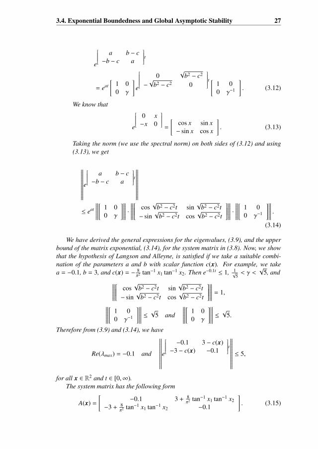
We have derived the general expressions for the eigenvalues, (3.9), and the upperbound of the matrix exponential, (3.14), for the system matrix in (3.8). Now, we showthat the hypothesis of Langson and Alleyne, is satisfied if we take a suitable combi-nation of the parameters a and b with scalar function c(x). For example, we takea = −0.1, b = 3, and c(x) = − 8
π2 tan−1 x1 tan−1 x2. Then e−0.1t ≤ 1, 1√
5< γ <
√5, and∥∥∥∥∥∥
cos√
b2 − c2t sin√
b2 − c2t− sin
√b2 − c2t cos
√b2 − c2t
∥∥∥∥∥∥ = 1,
∥∥∥∥∥∥[
1 00 γ−1
]∥∥∥∥∥∥ ≤ √5 and
∥∥∥∥∥∥[
1 00 γ
]∥∥∥∥∥∥ ≤ √5.
Therefore from (3.9) and (3.14), we have
Re(λmax) = −0.1 and
∥∥∥∥∥∥∥∥∥∥∥e
−0.1 3 − c(x)−3 − c(x) −0.1
t∥∥∥∥∥∥∥∥∥∥∥ ≤ 5,
for all x ∈ R2 and t ∈ [0,∞).The system matrix has the following form
A(x) =
[−0.1 3 + 8
π2 tan−1 x1 tan−1 x2
−3 + 8π2 tan−1 x1 tan−1 x2 −0.1
]. (3.15)

28 Chapter 3. SDC Parametrization and Stability Analysis
It is clear from the foregoing discussion that the system matrix in (3.15) is continu-ous, asymptotically stable (Hurwitz), and exponentially bounded. Thus the hypothesisof Langson and Alleyne is satisfied.
−2 −1 0 1 2 3
−4
−3
−2
−1
0
1
2
3xy−trajectories
State x1
Sta
te x
2
Figure 3.1: Phase-portrait of the system dynamics (3.8)
Fig. 3.1 shows the phase-portrait of the system dynamics in (3.8) using the systemmatrix (3.15) with an initial condition, x0 = [1.2 0]T . It indicates that the states ofthe system move away from the origin as time goes to infinity although the coefficientmatrix satisfies the sufficient conditions (as claimed in [47]) for global asymptoticstability. N
3.5 Periodicity and Global Asymptotic StabilityFrom the counterexample in the previous section, it is clear that the hypothesis ofLangson and Alleyne is not sufficient to endorse global asymptotic stability of non-linear systems of the form (3.2). At this point, a natural question is, what additionalconditions would be required to establish global asymptotic stability of nonlinear sys-tems of the form (3.2)? In addition to the smoothness conditions and exponentialboundedness, we study the case that A(x) is also a θ−periodic matrix, i.e.,
A(x) = A(x + θ) for all x ∈ Ω and some θ ∈ R. (3.16)
Condition C.4, that the system matrix A(x) is periodic, ensures that the finite escapetime phenomenon will not occur. If a function is continuous and periodic on Ω then it

3.5. Periodicity and Global Asymptotic Stability 29
must be bounded. In the following proposition, we prove how the periodicity conditionrules out the possibility of the finite escape time phenomenon.
Proposition 3.5.1. Suppose that the system (3.2) satisfies the usual regularity (smooth-ness) conditions. If the system matrix in (3.2) is continuous, Hurwitz and periodic thenthe system has bounded solutions for all times t < ∞.
Proof. The solution of (3.2) exists, because regularity conditions are assumed to besatisfied, and can be written as
x(t) = x0 +
∫ t
0A(x(s))x(s)ds. (3.17)
Since the system matrix A(x) is continuous, Hurwitz, and periodic for all x ∈ Ω, itmust be bounded. Therefore, ∃M > 0, s.t. ||A(x)|| < M, ∀x ∈ Rn. Taking the normon both sides of (3.17) and using the fact that A(x) is bounded, it follows that
||x(t)|| ≤ ||x0|| +
∫ t
0M||x(s)||ds.
Using Gronwall’s Lemma [85, Chapter 1, page:5], we get||x(t)|| ≤ ||x0||eMt.
This expression shows that the state of the system is bounded for all t < ∞, i.e., thestate does not blow up in finite time. This completes the proof.
Further research on this topic results in yet another counterexample which leadsus to the conclusion that adding the periodicity condition alone does not suffice toguarantee global asymptotic stability. The details are explained in the following sub-section.
3.5.1 A Counterexample Showing that the Periodicity of the Sys-tem Matrix does not Guarantee Global Asymptotic Stability
Example 3.5.1. This example has two parts: first we analyze the system matrix andthen analyze the corresponding system.
Analysis of Coefficient Matrix
In order to present the counterexample, we first consider the matrix
A(x1) =
(2α −2
2 + 4α2 −4α
), (3.18)
where α = sin2 x1 + ε, with ε ∈ R such that 0 < ε < 1. Hence, α is a real number suchthat 0 < α ≤ 1 + ε < 2 for any x1 ∈ R.
Note that the matrix A(x1) is periodic with period π, i.e., A(x1) = A(x1 + π) for allx1 ∈ R. Further, note that A(x1) depends on x1 in a continuous way.
With ε as above, the eigenvalues of A(x1) are given byλ1,2 = −α ± i
√4 − α2,

30 Chapter 3. SDC Parametrization and Stability Analysis
where “i” denotes the imaginary unit. Clearly, the eigenvalues of A(x1) are complex,since 4 − α2 > 0. Furthermore, the eigenvalues of A(x1) are located in the open lefthalf of the complex plane, since α > 0. Hence, for all x1 ∈ R, the matrix A(x1) is aso-called Hurwitz matrix, i.e., all eigenvalues of A(x1) have a negative real part.
An eigenvector for the eigenvalue λ1 = −α + i√
4 − α2 is given, for instance, bythe nonzero complex-valued vector
v1 =
(2
3α
)+ i
(0
−√
4 − α2
).
It can indeed be verified that A(x1)v1 = λ1v1. Note that A(x1) is a real-valuedmatrix, but that A(x1)v1 and λ1v1 are complex-valued expressions. Then, equating thereal and imaginary parts of A(x1)v1 and λ1v1, it follows that
A(x1)(
23α
)= −α
(2
3α
)−√
4 − α2
(0
−√
4 − α2
)and
A(x1)(
0−√
4 − α2
)=√
4 − α2
(2
3α
)− α
(0
−√
4 − α2
).
Combining the expressions, it follows that
A(x1)(
2 03α −
√4 − α2
)=
(2 0
3α −√
4 − α2
) −α√
4 − α2
−√
4 − α2 −α
,or
A(x1)T = T D,
with
T =
(2 0
3α −√
4 − α2
), D =
−α√
4 − α2
−√
4 − α2 −α
.By the restrictions on ε and α, it is clear that matrix T is invertible. Hence, it
follows thatA(x1) = T DT−1,
and, consequently, thateA(x1)t = TeDtT−1. (3.19)
Because of the special form of the matrix D, it follows (see any book on differentialequations such as [10, page. 332]) that for all t ≥ 0,
eDt = e−αt
cos√
4 − α2t sin√
4 − α2t− sin
√4 − α2t cos
√4 − α2t
.The matrix on the right-hand side in the above equation has a finite norm. Indeed,
considering the Frobenius norm, i.e., the square root of the sum of squared moduli ofall matrix elements, see [33], it follows that the Frobenius norm of the real matrix cos
√4 − α2t sin
√4 − α2t
− sin√
4 − α2t cos√
4 − α2t
,is equal to
√2. The Frobenius norm of eDt is then given by
√2e−αt. The Frobenius
norms of the matrices T and T−1 are given by√
8 + 8α2 and√
2+2α2
4−α2 , respectively.
3.5. Periodicity and Global Asymptotic Stability 31
Let ·||F denote the Frobenius norm. It is well-known (or easy to prove) that theFrobenius norm is sub-multiplicative, i.e., ||UV ||F ≤ ||U ||F ||V ||F for any two squarematrices U and V of the same size. Therefore, it follows from (3.19) that for all t ≥ 0,∥∥∥eA(x1)t
∥∥∥F ≤ ‖T‖F
∥∥∥eDt∥∥∥
F
∥∥∥T−1∥∥∥
F ≤√
8 + 8(1 + ε)2√
2e−αt
√2 + 2(1 + ε)2
4 − (1 + ε)2 .
Since α > 0, it follows that 0 ≤ e−αt ≤ 1, for all t ≥ 0. Hence, for all t ≥ 0,∥∥∥eA(x1)t∥∥∥
F ≤ 2√
2(2 + 2(1 + ε)2)√
4 − (1 + ε)2.
So, there exists a number M ∈ R, depending on ε, such that∥∥∥eA(x1)t
∥∥∥F ≤ M, for all
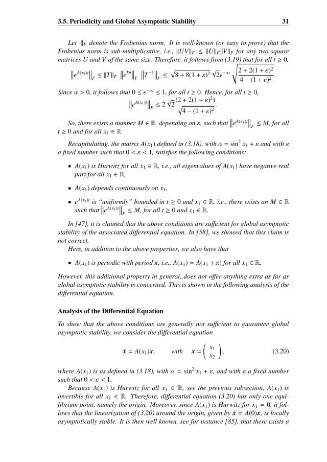
t ≥ 0 and for all x1 ∈ R.
Recapitulating, the matrix A(x1) defined in (3.18), with α = sin2 x1 + ε and with εa fixed number such that 0 < ε < 1, satisfies the following conditions:
• A(x1) is Hurwitz for all x1 ∈ R, i.e., all eigenvalues of A(x1) have negative realpart for all x1 ∈ R,
• A(x1) depends continuously on x1,
• eA(x1)t is “uniformly” bounded in t ≥ 0 and x1 ∈ R, i.e., there exists an M ∈ Rsuch that
∥∥∥eA(x1)t∥∥∥
F ≤ M, for all t ≥ 0 and x1 ∈ R.
In [47], it is claimed that the above conditions are sufficient for global asymptoticstability of the associated differential equation. In [58], we showed that this claim isnot correct.
Here, in addition to the above properties, we also have that
• A(x1) is periodic with period π, i.e., A(x1) = A(x1 + π) for all x1 ∈ R.
However, this additional property in general, does not offer anything extra as far asglobal asymptotic stability is concerned. This is shown in the following analysis of thedifferential equation.
Analysis of the Differential Equation
To show that the above conditions are generally not sufficient to guarantee globalasymptotic stability, we consider the differential equation
x = A(x1)x, with x =
(x1
x2
), (3.20)
where A(x1) is as defined in (3.18), with α = sin2 x1 + ε, and with ε a fixed numbersuch that 0 < ε < 1.
Because A(x1) is Hurwitz for all x1 ∈ R, see the previous subsection, A(x1) isinvertible for all x1 ∈ R. Therefore, differential equation (3.20) has only one equi-librium point, namely the origin. Moreover, since A(x1) is Hurwitz for x1 = 0, it fol-lows that the linearization of (3.20) around the origin, given by x = A(0)x, is locallyasymptotically stable. It is then well known, see for instance [85], that there exists a
32 Chapter 3. SDC Parametrization and Stability Analysis
neighborhood of the origin such that solutions of (3.20), starting in this neighborhood,converge to the origin for time going to infinity. However due to the non-linearity of(3.20), and often also in general, there are initial conditions for which this conver-gence does not take place. Indeed, as numerical simulations show, there are initialconditions such that the resulting solution does not converge.
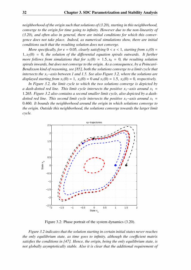
More specifically, for ε = 0.05, clearly satisfying 0 < ε < 1, starting from x1(0) =
1, x2(0) = 0, the solution of the differential equation spirals outwards. It furthermore follows from simulations that for x1(0) = 1.5, x0 = 0, the resulting solutionspirals inwards, but does not converge to the origin. As a consequence, by a Poincare-Bendixson kind of reasoning, see [85], both the solutions converge to a limit cycle thatintersects the x1−axis between 1 and 1.5. See also Figure 3.2, where the solutions aredisplayed starting from x1(0) = 1, x2(0) = 0 and x1(0) = 1.5, x2(0) = 0, respectively.
In Figure 3.2, the limit cycle to which the two solutions converge is depicted bya dash-dotted red line. This limit cycle intersects the positive x1−axis around x1 =
1.265. Figure 3.2 also contains a second smaller limit cycle, also depicted by a dash-dotted red line. This second limit cycle intersects the positive x1−axis around x1 =
0.460. It bounds the neighborhood around the origin in which solutions converge tothe origin. Outside this neighborhood, the solutions converge towards the larger limitcycle.
−2 −1.5 −1 −0.5 0 0.5 1 1.5 2−2.5
−2
−1.5
−1
−0.5
0
0.5
1
1.5
2
2.5xy−trajectories
State x1
Sta
te x
2
Figure 3.2: Phase portrait of the system dynamics (3.20).
Figure 3.2 indicates that the solution starting in certain initial states never reachesthe only equilibrium state, as time goes to infinity, although the coefficient matrixsatisfies the conditions in [47]. Hence, the origin, being the only equilibrium state, isnot globally asymptotically stable. Also it is clear that the additional requirement of

3.6. An LMI Based Approach for Global Asymptotic Stability 33
periodic state dependency of the coefficient matrix does not help in attaining globalasymptotic stability.
Concluding Remarks
From the foregoing discussion, it is clear that the conditions C.1, C.2, and C.3 are notsufficient to guarantee global asymptotic stability of a non-linear system written as apseudo-linear system in state dependent coefficient form (3.2), even with the periodic-ity condition as well, see [58]. N
3.6 An LMI Based Approach for Global AsymptoticStability
In general, periodicity of the system matrix does not imply global asymptotic stabilityof (3.2). However, this assumption helps in analyzing its global asymptotic stability aswe have seen in Example 3.5.1. For instance, we assume that the system matrix A(x)is a function of a single state component and it is θ−periodic as well. Then (3.16)becomes
A(x1 + θ) = A(x1), for all x1 ∈ R and θ ∈ R, (3.21)
where, without loss of generality, x1 is the first component of the state vector.The eigenvalue criterion is a well-known approach to analyze asymptotic stability
of linear systems. It is stated as follows [15, Chapter 7, page:203].
Theorem 3.6.1. Eigenvalue Criterion for Stability. The system
x = Ax, x(0) = x0, (3.22)
is asymptotically stable if and only if all the eigenvalues of the matrix A have negativereal parts.
Before the advent of fast computing machines like modern age computers, compu-tation of eigenvalues was a cumbersome task. In 1892, a Russian mathematician, A.M. Lyapunov (1857-1918) proposed a method to analyze asymptotic stability of linearsystems. This method does not require eigenvalue computation. Lyapunov narratedhis method as follows [15, Chapter 7, page:205].
Theorem 3.6.2. Lyapunov Stability Theorem. The system (3.22) is asymptoticallystable if and only if, for any symmetric positive definite matrix Q, there exists a uniquesymmetric positive definite matrix P satisfying the equation:
PA + AT P = −Q. (3.23)
In (3.23), we can easily transform the matrix equation into a matrix inequality toget
PA + AT P ≺ 0, ∵ −Q ≺ 0. (3.24)

34 Chapter 3. SDC Parametrization and Stability Analysis
For a given N × N matrix P, the constraint P() 0 would denote that the matrix P ispositive (semi-)definite and the constraint P() ≺ 0 would denote that the matrix P isnegative (semi-)definite.
In this section, an LMI based approach is proposed and discussed to establishglobal asymptotic stability of the pseudo-linear systems of the form (3.2) when thesystem matrix has the form (3.21). The motivation for this approach comes from[71, Chapter 4] where asymptotic stability of linear systems is analyzed subject toparameter uncertainties. We see a similar situation in (3.21) where the system matrixdepends on a single state component which varies periodically with period θ.
This approach has two steps. The first step is to formulate an LMI feasibilityproblem using the concept introduced in the Theorem 3.6.2. The solution of this LMIfeasibility problem gives a constant symmetric positive definite matrix. In the secondstep, we use the solution matrix from the LMI feasibility problem (Step I) to provethe global asymptotic stability of the system under consideration by using a quadraticLyapunov function. The details of this approach are as follows.
Step I- LMI Feasibility Problem Formulation
Inspired by the Lyapunov Stability Theorem, we propose an equivalent result for thepseudo-linear system (3.2). Before proceeding further, it is important to mention thatthe LMI solver SeDuMi which we use in the sequel, does not distinguish between and (likewise between ≺ and ). Therefore, we formulate the LMI feasibility prob-lem with non-strict equality constraints. The system (3.2) is pointwise asymptoticallystable if and only if for each x1 ∈ R, ∃ P(x1) = PT (x1) 0 s.t.
AT (x1)P(x1) + P(x1)A(x1) + In 0. (3.25)
It is important to mention that, without loss of generality, we take Q = In as a constantidentity matrix. The choice Q = In helps us in stability analysis by ensuring strictinequalities, as we will see in the sequel. Intuitively, we are interested to investigatewhether there exists a constant matrix P = PT 0 for which the following holds
AT (x1)P + PA(x1) + In 0, ∀ x1 ∈ R. (3.26)
Therefore, if the LMI in (3.26) holds true for all x1 in the principal interval [− θ2 ,θ2 ]
then it will hold for all x1 ∈ R.To verify this we proceed as follows. We mark k (sufficiently large) number of
points on [− θ2 ,θ2 ) and formulate an LMI feasibility problem as follows:
Does there exist a P = PT 0 which satisfies the LMI in (3.26) at k points, x1k ∈
[− θ2 ,θ2 )?
This gives rise to k + 1 LMIs. The system matrix A(x1) is θ-periodic which means thatit will be same at x1 = − θ2 and x1 = θ
2 . Hence, to ensure that all LMIs are distinct,we take x1k ∈ [− θ2 ,
θ2 ). Mathematically, we formulate the LMI feasibility problem as
follows:
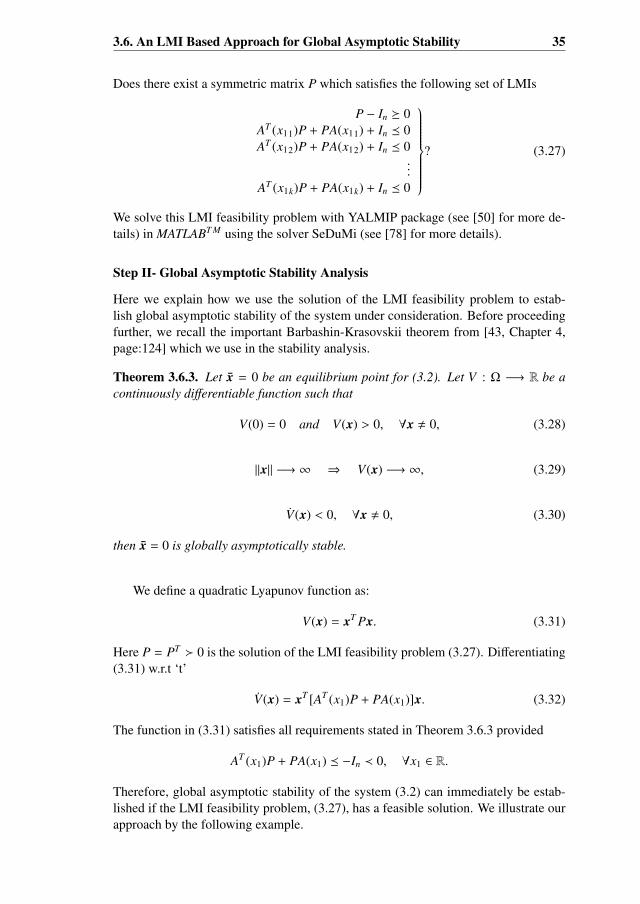
3.6. An LMI Based Approach for Global Asymptotic Stability 35
Does there exist a symmetric matrix P which satisfies the following set of LMIs
P − In 0AT (x11)P + PA(x11) + In 0AT (x12)P + PA(x12) + In 0
...
AT (x1k)P + PA(x1k) + In 0
? (3.27)
We solve this LMI feasibility problem with YALMIP package (see [50] for more de-tails) in MATLABT M using the solver SeDuMi (see [78] for more details).
Step II- Global Asymptotic Stability Analysis
Here we explain how we use the solution of the LMI feasibility problem to estab-lish global asymptotic stability of the system under consideration. Before proceedingfurther, we recall the important Barbashin-Krasovskii theorem from [43, Chapter 4,page:124] which we use in the stability analysis.
Theorem 3.6.3. Let x = 0 be an equilibrium point for (3.2). Let V : Ω −→ R be acontinuously differentiable function such that
V(0) = 0 and V(x) > 0, ∀x , 0, (3.28)
||x|| −→ ∞ ⇒ V(x) −→ ∞, (3.29)
V(x) < 0, ∀x , 0, (3.30)
then x = 0 is globally asymptotically stable.
We define a quadratic Lyapunov function as:
V(x) = xT Px. (3.31)
Here P = PT 0 is the solution of the LMI feasibility problem (3.27). Differentiating(3.31) w.r.t ‘t’
V(x) = xT [AT (x1)P + PA(x1)]x. (3.32)
The function in (3.31) satisfies all requirements stated in Theorem 3.6.3 provided
AT (x1)P + PA(x1) −In ≺ 0, ∀x1 ∈ R.
Therefore, global asymptotic stability of the system (3.2) can immediately be estab-lished if the LMI feasibility problem, (3.27), has a feasible solution. We illustrate ourapproach by the following example.

36 Chapter 3. SDC Parametrization and Stability Analysis
Example 3.6.1. We consider a fourth order nonlinear system of the form (3.2). Webegin by defining a system matrix of the following form.
A(x1) = A0 + A1 cos x1 + B1 sin x1. (3.33)
We generate the constant matrices A0, A1, and B1 at random using the standard Gaus-sian distribution with mean 0 and standard deviation 1. In particular, we randomlygenerate A0 as a diagonal matrix and A1 and B1 as full matrices. Thus we form asystem matrix which is continuous and periodic. To obtain a continuous, periodic,and Hurwitz matrix, we define,
βM= (1 + δ)λmax(A(x1)), ∀x1 ∈ [−π, π], (3.34)
where δ > 0 is a small number and λmax denotes the maximum real part of the eigen-values of A(x1). Then the matrix
A(x1) = A(x1) − βI, (3.35)
where I is the identity matrix of the size of A(x1), will be Hurwitz. Figure 3.3 showsthe behavior of the state dynamics of a system of the form (3.2), having system matrix(3.35) and A0, A1, and B1 are as given later in this example, with four different arbi-trarily chosen initial conditions. We see that the states converge asymptotically to theorigin. This indicates that the states of the system may converge asymptotically to theorigin for all initial conditions x0 = (x1, x2, x3, x4) ∈ R4.
In retrospect of the theory discussed earlier, the first step is to formulate an LMIfeasibility problem. We present three different results each with a different choice of thenumber of LMIs in the feasibility problem. The system matrix (3.35) is 2π− periodic.We mark (k =)120, 300, and 440 points on the interval [−π, π). In this way, we form asystem of 121, 301, and 441 LMIs analogous to (3.27). As has been mentioned earlier,we generate the set of matrices A0, A1, and B1 at random. We see in our experimentsthat for all such sets of matrices, the state dynamics of the nonlinear system, witharbitrarily chosen initial states, converge asymptotically to the origin. In a particularset, we have the following matrices
A0 =
0.3146 0 0 0
0 0.8596 0 00 0 0.1287 00 0 0 0.0166
,
A1 =
−0.0728 0.9884 0.6450 0.2224−0.9943 −0.5990 −1.3099 1.8713−0.7474 1.4766 −0.8674 0.1100−0.0308 −0.8138 −0.4742 −0.4113
,
B1 =
0.5112 −0.2958 1.6777 0.3630−1.1991 −0.1680 1.9969 −0.5670−0.0964 0.1795 0.6970 −1.04420.4458 0.4211 −1.3664 0.6971
.
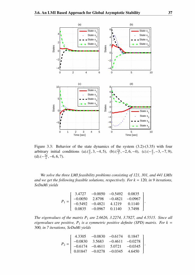
3.6. An LMI Based Approach for Global Asymptotic Stability 37
0 2 4 6
−4
−2
0
2
4
Sta
tes
(a)
State x
1
State x2
State x3
State x4
0 5 10
−4
−2
0
2
4
6
Sta
tes
(b)
State x
1
State x2
State x3
State x4
0 1 2 3 4 5
−5
0
5
10
Time [sec]
Sta
tes
(c)
State x
1
State x2
State x3
State x4
0 5 10
−8
−6
−4
−2
0
2
4
6
8
Time [sec]
Sta
tes
(d)
State x1
State x2
State x3
State x4
Figure 3.3: Behavior of the state dynamics of the system (3.2)-(3.35) with fourarbitrary initial conditions (a).( π5 , 3,−4, 5), (b).( 2π
5 ,−2, 6,−4), (c).(− π2 ,−3,−7, 9),(d).(− 3π
4 ,−6, 6, 7).
We solve the three LMI feasibility problems consisting of 121, 301, and 441 LMIsand we get the following feasible solutions, respectively. For k = 120, in 9 iterations,SeDuMi yields
P1 =
3.4727 −0.0050 −0.5492 0.0835−0.0050 2.8798 −0.4821 −0.0967−0.5492 −0.4821 4.1219 0.11400.0835 −0.0967 0.1140 3.7498
.The eigenvalues of the matrix P1 are 2.6626, 3.2274, 3.7827, and 4.5515. Since alleigenvalues are positive, P1 is a symmetric positive definite (SPD) matrix. For k =
300, in 7 iterations, SeDuMi yields
P2 =
4.3305 −0.0830 −0.6174 0.1847−0.0830 3.5683 −0.4611 −0.0278−0.6174 −0.4611 5.0721 −0.03450.01847 −0.0278 −0.0345 4.6450
.
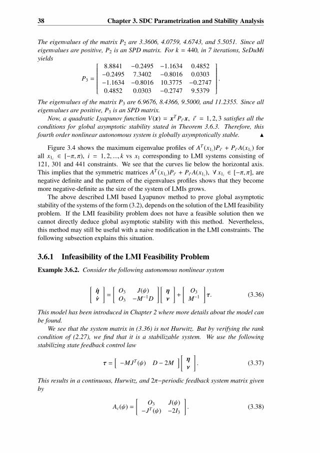
38 Chapter 3. SDC Parametrization and Stability Analysis
The eigenvalues of the matrix P2 are 3.3606, 4.0759, 4.6743, and 5.5051. Since alleigenvalues are positive, P2 is an SPD matrix. For k = 440, in 7 iterations, SeDuMiyields
P3 =
8.8841 −0.2495 −1.1634 0.4852−0.2495 7.3402 −0.8016 0.0303−1.1634 −0.8016 10.3775 −0.27470.4852 0.0303 −0.2747 9.5379
.The eigenvalues of the matrix P3 are 6.9676, 8.4366, 9.5000, and 11.2355. Since alleigenvalues are positive, P3 is an SPD matrix.
Now, a quadratic Lyapunov function V(x) = xT Pi′ x, i′ = 1, 2, 3 satisfies all theconditions for global asymptotic stability stated in Theorem 3.6.3. Therefore, thisfourth order nonlinear autonomous system is globally asymptotically stable. N
Figure 3.4 shows the maximum eigenvalue profiles of AT (x1i )Pi′ + Pi′A(x1i ) forall x1i ∈ [−π, π), i = 1, 2, ..., k vs x1 corresponding to LMI systems consisting of121, 301 and 441 constraints. We see that the curves lie below the horizontal axis.This implies that the symmetric matrices AT (x1i )Pi′ + Pi′A(x1i ), ∀ x1i ∈ [−π, π], arenegative definite and the pattern of the eigenvalues profiles shows that they becomemore negative-definite as the size of the system of LMIs grows.
The above described LMI based Lyapunov method to prove global asymptoticstability of the systems of the form (3.2), depends on the solution of the LMI feasibilityproblem. If the LMI feasibility problem does not have a feasible solution then wecannot directly deduce global asymptotic stability with this method. Nevertheless,this method may still be useful with a naive modification in the LMI constraints. Thefollowing subsection explains this situation.
3.6.1 Infeasibility of the LMI Feasibility ProblemExample 3.6.2. Consider the following autonomous nonlinear system
[ην
]=
[O3 J(ψ)O3 −M−1D
] [ην
]+
[O3
M−1
]τ. (3.36)
This model has been introduced in Chapter 2 where more details about the model canbe found.
We see that the system matrix in (3.36) is not Hurwitz. But by verifying the rankcondition of (2.27), we find that it is a stabilizable system. We use the followingstabilizing state feedback control law
τ =[−MJT (ψ) D − 2M
] [ ην
]. (3.37)
This results in a continuous, Hurwitz, and 2π−periodic feedback system matrix givenby
Ac(ψ) =
[O3 J(ψ)−JT (ψ) −2I3
]. (3.38)
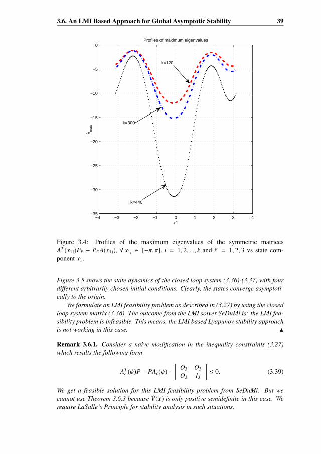
3.6. An LMI Based Approach for Global Asymptotic Stability 39
−4 −3 −2 −1 0 1 2 3 4−35
−30
−25
−20
−15
−10
−5
0
x1
λ max
Profiles of maximum eigenvalues
k=120
k=300
k=440
Figure 3.4: Profiles of the maximum eigenvalues of the symmetric matricesAT (x1i)Pi′ + Pi′A(x1i), ∀ x1i ∈ [−π, π], i = 1, 2, ..., k and i′ = 1, 2, 3 vs state com-ponent x1.
Figure 3.5 shows the state dynamics of the closed loop system (3.36)-(3.37) with fourdifferent arbitrarily chosen initial conditions. Clearly, the states converge asymptoti-cally to the origin.
We formulate an LMI feasibility problem as described in (3.27) by using the closedloop system matrix (3.38). The outcome from the LMI solver SeDuMi is: the LMI fea-sibility problem is infeasible. This means, the LMI based Lyapunov stability approachis not working in this case. N
Remark 3.6.1. Consider a naive modification in the inequality constraints (3.27)which results the following form
ATc (ψ)P + PAc(ψ) +
[O3 O3
O3 I3
] 0. (3.39)
We get a feasible solution for this LMI feasibility problem from SeDuMi. But wecannot use Theorem 3.6.3 because V(x) is only positive semidefinite in this case. Werequire LaSalle’s Principle for stability analysis in such situations.

40 Chapter 3. SDC Parametrization and Stability Analysis
0 5 10−1.5
−1
−0.5
0
0.5
1
1.5
2
2.5
Sta
tes
(a)
0 5 10
−2
−1
0
1
2
Sta
tes
(b)
0 5 10−3
−2
−1
0
1
Time [sec]
Sta
tes
(c)
0 5 10
−10
−5
0
5
Time [sec]
Sta
tes
(d)
xyψuvr
xyψuvr
xy
ψuvr
xy
ψuvr
Figure 3.5: Behavior of the state dynamics of the system in Example3.6.1 with four arbitrary initial conditions (a).(2, 2, π6 , 0, 0, 0), (b).(2,−2, π3 , 0, 0, 0),(c).(−1,−1,− 8π
9 , 0, 0, 0), (d).(−10, 4,− 2π3 , 4,−3, 4).
Remark 3.6.2. A more practical and useful form of (3.37) can be
τ =[−MJT (ψ) R − 2M
] [ ην
], (3.40)
where R denotes the additional damping effect introduced via controller action.
To investigate the infeasibility issue in more detail, an analytic approach to theLMI feasibility problem associated with the system in Example 3.6.2, is presented inthe following subsection.
Analytic approach to the LMI problem
For the closed loop system matrix (3.38), we would like to find an SPD matrix P s.t.
ATc (ψ)P + PAc(ψ) ≺ 0, ∀ψ ∈ [−π, π].
Suppose that P has the following form
P =
[Pa PT
bPb Pc
].
3.6. An LMI Based Approach for Global Asymptotic Stability 41
For the sake of convenience, from here onward in this subsection, we omit the argu-ment ψ from J(ψ). Now consider,
ATc P + PAc ≺ 0,
⇐⇒
[O3 −JJT −2I3
] [Pa PT
bPb Pc
]+
[Pa PT
bPb Pc
] [O3 J−JT −2I3
]≺ 0,
⇐⇒
[−JPb − (JPb)T PaJ − 2PT
b − JPc
(PaJ − 2PTb − JPc)T (PbJ)T + PbJ − 4Pc
]≺ 0. (3.41)
Or equivalently,
⇐⇒ −
[−JPb − (JPb)T PaJ − 2PT
b − JPc
(PaJ − 2PTb − JPc)T (PbJ)T + PbJ − 4Pc
] 0. (3.42)
It is a well-known fact that a symmetric matrix is positive definite if and only if all theleading principal minors of the matrix are positive, see [43]. Therefore, we focus onthe leading principal block diagonal entry
−JPb − (JPb)T .
The inequality 3.42 holds true only if
JPb + (JPb)T 0, ∀ψ ∈ [−π, π]. (3.43)
In the sequel, we show that the necessary condition (3.43) for (3.42) to hold true, doesnot hold.
Consider Pb in the following form
Pb =
[Pb11 ∗
∗ ∗
],
where Pb11 is a 2 × 2 block entry while the entries of Pb which are not relevant for theanalysis are marked by asterisks. Since (3.43) must be true for all ψ ∈ [−π, π], we takethe following two cases:
Case 1. ψ = 0,
JPb + (JPb)T =
[Pb11 + PT
b11∗
∗ ∗
].
Case 2. ψ = π,
JPb + (JPb)T =
[−Pb11 − PT
b11∗
∗ ∗
].
Now the inequality (3.43) holds only if the following holds
Pb11 + PTb11 0 and − Pb11 − PT
b11 0.
42 Chapter 3. SDC Parametrization and Stability Analysis
This is an improbable scenario. Therefore, about the LMI feasibility problem of Ex-ample 3.6.2, we conclude the following
“@ P = PT 0 s.t. ATc (ψ)P + PAc(ψ) ≺ 0, holds true for all ψ ∈ [−π, π].”
In the foregoing discussion, we have proved analytically that the LMI problemcorresponding to the system (3.36) has no solution. In the following, we continuewith global stability analysis of the system (3.36) by using Lyapunov stability theoryand LaSalle’s invariance theorem.
3.6.2 Further Analysis for Global Asymptotic StabilityBefore proceeding further, we recall an important result from stability theory whichwas first formulated by J. P. LaSalle, see Appendix B for more details. It is stated asfollows [43, Chapter 4, page:128]:
Theorem 3.6.4. The LaSalle’s Invariance Theorem (Principle). Let Ω0 ⊂ Ω be a com-pact set that is positively invariant with respect to a nonlinear system: x = f (x), x0 =
x(t0). Let V : Ω −→ R be a continuously differentiable function such that V(x) ≤ 0 inΩ0. Let E be the set of all points in Ω0 where V(x) = 0. Let M be the largest invariantset in E. Then every solution starting in Ω0 approaches M as t → ∞.
An invariant set is defined as:
Definition 3.6.1. (Invariant Set) A set M is an invariant set for a dynamic systemif every system trajectory which starts from a point in M remains in M for all futuretime.
The system matrix (3.38) has a special structure with a skew symmetric part. Wetry to use this structure to analyze global asymptotic stability of the system. Let usconsider a Lyapunov function of the form
V(x) = xT x. (3.44)
Differentiating the Lyapunov function, we get
V(x) = xT[
O3 J(ψ)−JT (ψ) −2I3
]x,
⇒ V(x) = −4νTν,
⇒ V(x) ≤ 0, ∀ x , 0.
Now,
V(x) = 0, ⇒ ν = 0, and η is arbitrary.
Therefore,
El = x : V(x) = 0
= ν = 0, η is free.

3.7. Summary and Conclusions 43
The next step is to find the largest invariant subset of El. Suppose η(t) and ν(t) is asolution pair of closed loop system (3.36) and (3.37) that belongs identically to El.Then
ν(t) ≡ 0, ⇒ ν(t) ≡ 0,
⇒ −JT (ψ)η(t) ≡ 0,
⇒ η(t) ≡ 0. (3.45)
Therefore, from (3.45), we conclude that the only solution of the closed loop sys-tem (3.36) and (3.37) which stays identically in El, is the trivial solution. Hence(η, ν) = (0, 0) is a globally asymptotically stable equilibrium point of the the closedloop system (3.36) and (3.37) .
3.7 Summary and Conclusions
This chapter focuses on the stability analysis of a special type of nonlinear systems.They can be transformed to pseudo-linear form by using the SDC framework. Thesystem matrix in the new representation depends on a single state variable. Localasymptotic stability is easy to analyze but the major topic of interest in this chapteris global asymptotic stability analysis. We start with a brief review of the past resultson this topic. The main contributions are two counterexamples. Example 3.4.1 showsthat the exponential boundedness of the system matrix together with the continuity andHurwitzness conditions does not imply global asymptotic stability of the nonlineardynamical system (3.2). Example 3.5.1 shows that, in addition, even if the periodicityof the system matrix is assumed, it does not ensure global asymptotic stability of (3.2).
However, as a consequence of the periodicity of the system matrix, we introduceanother method to prove the global asymptotic stability of the pseudo-linear system(3.2). This method combines the concepts of the Lyapunov stability theory and theLMIs. This approach is motivated from the idea of LPV approach introduced in [71]to the pseudo-linear systems of the form (3.2). We use the periodicity of the systemmatrix together with the Lyapunov stability theory and the LMIs to formulate an LMIfeasibility problem. This LMI feasibility problem is solved by using the YALMIPinterface under MATLAB. YALMIP uses SeDuMi (an LMI solver) which transformsthe LMI feasibility problem into a convex optimization problem. The positive (semi-)definite solution of the LMI feasibility problem is then used to get a quadratic Lya-punov function. Global asymptotic stability is then followed by Lyapunov stabilitytheory.
We first explained this method by using an academic example of a fourth orderpseudo-linear system. Afterwards, we proceed to prove global asymptotic stability ofthe nominal vessel model (3.36) subject to a naive state feedback controller (3.37). Itturns out that the LMI feasibility problem associated with the closed loop system ma-trix (3.38) does not have a feasible solution. This outcome is then proved analytically.More investigation to this bottleneck revealed that a small modification in the LMIfeasibility problem, see (3.39), resolves this problem. The consequence of this mod-ification is that the derivative of the Lyapunov function will be positive semidefinite

44 Chapter 3. SDC Parametrization and Stability Analysis
in this situation. In this case, the LaSalle’s invariance principal is used to establishglobal asymptotic stability of the pseudo-linear system.
Chapter 4State Dependent Riccati EquationBased Control Design1
The use of DP systems for the positioning control of ships started in the early sixties.The first DP control system used the conventional PID type control law together
with a notch filter, to control each of the surge, sway, and yaw motions. The purpose ofthe notch filter was to filter out the effects of the WF motions from the feedback loop.There were two main disadvantages of this approach: the integral action of the PIDcontroller is very low due to the coupling between the surge, sway, and yaw motionsand there is a phase lag in the control loop due to the notch filter.
The disadvantages of the PID control law motivated a Norwegian company, Kongs-berg, to initiate efforts to invent new DP control systems using the concepts of optimalcontrol theory and Kalman filtering from the modern control theory. These effortsmade way for the modern concepts for wave filtering like state estimators or observers.Observers are more useful than the classical filtering techniques because they also giveestimates of the unknown states of the system.
Observer based wave filtering techniques have been reported by many researchers,for instance see [1], [29], and [51]. One such approach is reported in [74] and itis based on the state dependent algebraic Riccati equation, also known as SDARE.An SDARE observer is proposed to estimate the states of a DP vessel model. Thisobserver was then separately used in combination with a backstepping controller [74]and a PID controller [75].
In this chapter, we extend the ideas of LQR theory to address the nonlinear controldesign and estimation problems for the DP vessel. The nonlinear model of the vesselmotion described in Chapter 2 can be assumed as a pseudo-linear system by consid-ering the SDC parametrization which is discussed in Chapter 3. Our aim is to studythe SDARE controller and observer design techniques in connection with the controldesign problem of a DP vessel. The state dependent algebraic Riccati equation plays
1Part of this work has been published in the proceedings of the UKACC International Conference onControl (CONTROL 2010), see [57].
45
46 Chapter 4. SDARE-based control Design
a fundamental role in this theory. We will see that the SDARE controller is a statefeedback or an output feedback controller.
4.1 Optimal Control Problem and the SDAREWe mimick the LQR problem for the linear systems to address the control designproblem of the pseudo-linear vessel system. Let us start by defining the optimal con-trol (OC) or linear quadratic regulation (LQR) problem for the pseudo-linear systemdescribing the sea vessel motion. We adapt the definition of the LQR problem from[15] to customize it according to the pseudo-linear model under consideration.
Definition 4.1.1. (LQR/OC problem for pseudo-linear system of vessel model)Given matrices Q and R, find a control signal u(t) such that the quadratic cost function
J(x0,u(t)) =12
∫ ∞
t0
(xT (t)Qx(t) + uT (t)Ru(t)
)dt, (4.1)
is minimized, subject to
x = A(ψ)x(t) + Bu(t), x(t0) = x0. (4.2)
In (4.1) and (4.2), the n-dimensional vector x ∈ Rn describes the state of thesystem, Q = HT H ∈ Rn×n (HT ∈ Rn×p) is a symmetric positive semidefinite (SPSD)matrix, u ∈ Rm is the control input vector, R ∈ Rm×m is an SPD matrix, A(ψ) ∈ Rn×n isthe system matrix, and the matrix B ∈ Rn×m describes the controller configuration.
The matrices Q and R in (4.1) are called weighting or penalty matrices. Theseare also called the tuning parameters of the SDARE controller as the performanceof the SDARE controller can be manipulated by playing around with these matrices.Although we assume Q and R to be constant matrices, they can be state dependent aswell. Physically, the expression xT (t)Qx(t) describes the deviation of the state vectorfrom the origin (equilibrium state) and the expression uT (t)Ru(t) describes the controlcost.
In [7], it has been proved that the problem defined in Definition 4.1.1 has a subop-timal solution. The following theorem states this result.
Theorem 4.1.1. (The SDARE controller) Consider a nonlinear system in the SDCform
x = A(x)x + B(x)u. (4.3)
The SDC form implies that the matrices A(x) and B(x) are continuous in x for all||x|| ≤ r, r > 0, see Section 3.1. Assume further that the matrices A(x), B(x), and Qare such that the pair (H, A(x)) is detectable and the pair (A(x), B(x)) is stabilizablefor all x ∈ Ω ⊆ Br(0)2, where Ω is a nonempty neighborhood of the origin.
Then the system (4.3) with control
u(x) = −Kc(x)x, (4.4)
2Br(0) = x ∈ Rn : ||x|| < r
4.2. Control System Design for the DP Vessel 47
where the controller gain is
Kc(x) = R−1BT (x)Πc(x), (4.5)
is locally asymptotically stable. In (4.5), Πc(x) is the solution of the SDARE associatedwith (4.1) and (4.3), which is given by
Πc(x)A(x) + AT (x)Πc(x) + Q − Πc(x)B(x)R−1BT (x)Πc(x) = 0. (4.6)
Proof. See [7].
4.2 Control System Design for the DP VesselIn this section, we illustrate the SDARE-based controller and observer design tech-nique for the control system design of the DP vessel. A DP vessel model is given inChapter 2. The SDARE (4.6) in context of the vessel model becomes
Πc(ψ)A(ψ) + AT (ψ)Πc(ψ) + Q − Πc(ψ)BR−1BT Πc(ψ) = 0. (4.7)
This is a special SDARE in the sense that only the system matrix depends on stateand this state dependence too is only on a single state component in a periodic way.Many solutions of (4.7) could be possible, but the one which is positive (semi-)definiteis desired for most of the applications. The sufficient conditions for the pointwiseexistence of the solution of the SDARE (4.7) as given in [54], are: the pairs (A(ψ), B)and (H, A(ψ)) are, respectively, pointwise stabilizable and detectable for all ψ ∈ R.
We divide our study into two steps. First, we assume that there is no WF motion inthe measured output and only the LF motion is to be regulated. Later on, we assumethat the WF motion component is also present in the measured output.
4.2.1 Nonlinear Regulation Problem for the LF ModelThe LF motion as described in Chapter 2 is given by
η =J(ψ)η, (4.8)
ν = − M−1Dν + M−1JT (ψ)b + M−1τ, (4.9)
b = − T−1b + Ψwb, (4.10)
yb =Cbη + υ, (4.11)
where η = [x, y, ψ]T is position coordinate vector, ν = [u, v, r]T is velocity coordinatevector, b ∈ R3 describes the environmental disturbances, and τ represents the controlforces and torque. The vectors wb and υ represent the process and measurement noise,respectively. They are described by the zero-mean Gaussian white noise processes,i.e., wb ∼ N(0,Qc,b) and υ ∼ N(0,Rc). We study the LF motion regulation problem bydividing it in two parts. In the first part, we assume that the bias forces are completelygiven or their estimate is available. In the second part, we assume that slowly varyingbias forces and moments are unknown and hence should be estimated.
48 Chapter 4. SDARE-based control Design
I. Disturbance vector b is known
We assume that the disturbance vector b is known or its estimate b is available andthere is no measurement noise. The LF model in the SDC form may then be writtenas [
ην
]=
[O3 J(ψ)O3 −M−1D
] [ην
]+
[O3
M−1
]u +
[O3
M−1JT (ψ)
]b, (4.12)
yb =[
I3 O3
] [ ην
]. (4.13)
The corresponding controllability and observability matrices are given by
Cb =
[O3 J(ψ)M−1 · · · J(ψ)(−M−1D)4M−1
M−1 −M−1DM−1 · · · (−M−1D)5M−1
], (4.14)
and
Ob =
I3 O3
O3 J(ψ)...
...
O3 J(ψ)(−M−1D)4
. (4.15)
The matrices defined in (4.14) and (4.15) have full row and column ranks, respectively.Therefore, the system (4.12) is both pointwise controllable and observable. Therefore,by using Theorem 4.1.1, we define a locally asymptotically stable SDARE controllerfor (4.12) as follows
u = −R−1M−1[
Π21(ψ) Π22(ψ)] [ ην
]− JT (ψ)b. (4.16)
The control law (4.16) can be described as a state feedback law with a feedforwardterm ‘−JT (ψ)b’. Moreover, Π21(ψ) and Π22(ψ) comes from
Πc(ψ) =
[Π11(ψ) Π12(ψ)Π21(ψ) Π22(ψ)
]. (4.17)
which is the symmetric solution of the SDARE associated with (4.1) and (4.12). From(4.13), it is clear that we can only measure the position of the vessel and its velocitiesare not available for feedback. But we can also write (4.16) as
u = −R−1M−1[
Π21(ψ) Π22(ψ)JT (ψ)] [ ηη
]− JT (ψ)b. (4.18)
This control law can be seen as PD-type control law with feedforward term ‘−JT (ψ)b’.
Stability analysis of the controller (4.16)
The local asymptotic stability of the state feedback SDARE controller follows fromTheorem 4.1.1. We prove by using the LMI based technique discussed in Chapter

4.2. Control System Design for the DP Vessel 49
3 that the SDARE feedback controller stabilizes the vessel globally asymptoticallyaround the origin. We can write the SDARE state feedback controller, (4.16), as
u = −[
K1(ψ) K2(ψ)] [ ην
]− JT (ψ)b. (4.19)
The closed loop system (4.12) and (4.19) is given by[ην
]=
[O3 J(ψ)
−M−1K1(ψ) ∗
]︸ ︷︷ ︸
Acl(ψ)
[ην
]. (4.20)
It is a well-known fact that the SDARE controller results in an asymptoticallystable closed loop matrix, see for instance [7]. Therefore, the closed loop systemmatrix (4.20) is pointwise Hurwitz. Using the LMI approach (see Chapter 3 for moredetails), it turns out that there exists an SPD matrix P such that
ATcl(ψ)P + PAcl(ψ) +
[0 00 I3
]≤ 0, ∀ψ ∈ [0, 2π]. (4.21)
Now we consider the quadratic Lyapunov function: V(x) = xT Px. Differentiatingw.r.t. ‘t’, we get
V(x) = xT (ATcl(ψ)P + PAcl(ψ))x,
≤ xT[
0 00 −I3
]x, using (4.21),
≤ −νTν,
≤ 0.
Since V(x) ≤ 0, therefore, we use LaSalle’s invariance principle to further analyzethe stability of the closed loop system. For this we first find the set of points whereV(x) = 0.
El = x : V(x) = 0,
= ν = 0, η is free.
Now we need the invariant sets of the closed loop system. To show that the origin isthe only equilibrium point of the closed loop system, we need to show that no solutionother than the trivial solution stays identically in El, i.e., η(t) ≡ 0 and ν(t) ≡ 0 for all‘t’.
Let η(t) and ν(t) be a solution pair of the closed loop system (4.20) that belongsidentically to El. Then
ν(t) ≡ 0, ⇒ ν(t) ≡ 0,
⇒ −M−1K1(ψ)η(t) ≡ 0. (4.22)
50 Chapter 4. SDARE-based control Design
To show that η(t) ≡ 0, we need to prove that K1(ψ) is a non-singular matrix. We provethis by contradiction. Suppose that it is singular then ∃ v , 0 such that
M−1K1(ψ)v = 0,
⇒
[O3 J(ψ)
−M−1K1(ψ) ∗
] [v0
]= 0
[v0
].
This implies that λ = 0 is an eigenvalue of the closed loop system matrix in (4.20).But it is a well-known fact that the closed system (4.20) is pointwise asymptoticallystable (all eigenvalues lie in the left half plane). Therefore, it is a contradiction. Hence,K1(ψ) is nonsingular.
Therefore, from (4.22), we conclude that the only solution of the closed loop sys-tem which stays identically in El is the trivial solution. Hence (η∗, ν∗) = (0, 0) is aglobally asymptotically stable equilibrium point of the the closed loop system (4.20)which means that the SDARE controller (4.19) globally asymptotically stabilizes thevessel.
II. Disturbance vector b is unknown
We now assume that the LF disturbances are slowly varying (as described by the firstorder Markov process b = −T−1b + Ψwb) but unknown and should be estimated. TheLF motion in this case, in the SDC form, is described as ηνb
=
O3 J(ψ) O3
O3 −M−1D M−1JT (ψ)O3 O3 −T−1
ηνb
+
O3
M−1
O3
u +
O3
O3
Ψ
wb, (4.23)
yb =[
I3 O3 O3
] ηνb + v. (4.24)
The controllability and observability matrices for (4.23)-(4.24) are given by
Cb =
O3 J(ψ)M−1 · · · J(ψ)(−M−1D)7M−1
M−1 −M−1DM−1 · · · (−M−1D)8M−1
O3 O3 · · · O3
, (4.25)
and
Ob =
I3 O3 O3
O3 J(ψ) O3
O3 −J(ψ)M−1D J(ψ)M−1JT (ψ)...
......
. (4.26)
Since the matrices M, D, and JT (ψ) are non-singular, the controllability matrix (4.25)has rank 6. This means that only the states η and ν are controllable. This is notrestrictive as the bias forces are always uncontrollable. The observability matrix (4.26)has full rank for all ψ ∈ R. An SDARE associated with (4.23) is given by
Πc(ψ)Ab(ψ) + ATb (ψ)Πc(ψ) + Q − Πc(ψ)BbR−1BT
b Πc(ψ) = 0. (4.27)

4.2. Control System Design for the DP Vessel 51
Using Theorem 4.1.1, a locally asymptotically stable SDARE-based suboptimalcontrol law is given by
u = −R−1M−1[
Π21(ψ) Π22(ψ) Π23(ψ)] ηνb
. (4.28)
The gain of the SDARE controller is defined by
Kc(ψ) = R−1M−1[
Π21(ψ) Π22(ψ) Π23(ψ)], (4.29)
where Π21(ψ), Π22(ψ), and Π23(ψ) are obtained from the solution of the SDARE (4.27).The control law (4.28) can be described as a state feedback controller. From (4.24), wenotice that only the LF position and heading can be measured by the sensors. There-fore, a state estimator is required to estimate the complete state. A suboptimal locallyasymptotically stable SDARE controller for the system (4.23)-(4.24) will be
u = −R−1M−1[
Π21(ψ) Π22(ψ) Π23(ψ)] ην
b
. (4.30)
Since the system (4.23)-(4.24) is pointwise observable, the corresponding dual systemwill be pointwise controllable. Therefore, we can design a suboptimal locally asymp-totically stable SDARE observer, see [7]. The following theorem states this result.
Theorem 4.2.1. (The SDARE state estimator) Assume that a system in SDC form
x = A(x)x + B(x)u, (4.31)
y = C(x)x, (4.32)
is such that f (x) = A(x)x and ∂ f (x)∂x j
, j = 1, 2, ..., n are continuous in x for all ||x|| ≤r, r > 0 and x = 0 is a stable equilibrium point of (4.31). Assume further that thepair (A(x),C(x)) is pointwise detectable and the matrices A(x) and C(x) are locallyLipschitz for all x ∈ Ω ⊆ Br(0), where Ω is a nonempty neighborhood of the origin.Then the estimated state given by
˙x = A(x)x + B(x)u + Ko(x)(y − y), (4.33)
will converge locally asymptotically to the state. In (4.33), Ko(x) is the observer gainand is given by
Ko(x) = Πo(x)CT V−1. (4.34)
In (4.34), Πo(x) is the solution of the dual SDARE
Πo(x)AT (x) + A(x)Πo(x) + U − Πo(x)CT V−1CΠo(x) = 0, (4.35)
associated with the system (4.31)-(4.32).
Proof. See [7].

52 Chapter 4. SDARE-based control Design
An SDARE observer for the system (4.23)-(4.24) is given by˙η˙ν˙b
=
O3 J(ψ) O3
O3 −M−1D M−1JT (ψ)O3 O3 −T−1
ην
b
+
O3
M−1
O3
u + Ko(ψ)(yη − yη), (4.36)
yη =[
I3 O3 O3
] ην
b
. (4.37)
The third term in (4.36) corrects the observer model by a nonlinear feedback of thedifference between the measured output yη and the estimated output yη. The observergain Ko(ψ) in (4.36) is defined by
Ko(ψ) =
Π11(ψ)Π21(ψ)Π31(ψ)
· V−1, (4.38)
where Πi1, i = 1, 2, 3 are obtained from the solution of the corresponding dual SDAREof the form (4.35).
So far we have defined a suboptimal locally asymptotically stable nonlinear con-trol law (4.30) and a suboptimal locally asymptotically stable nonlinear observer (4.36).A combination of both is called a nonlinear compensator. The separation propertiesfor combination of linear controllers and observers are well defined, see for instance[60]. The separation principles for the nonlinear compensators are not well establishedyet. The following theorem from [7] states one particular result about stability of anSDARE compensator.
Theorem 4.2.2. (The SDARE state compensator) Assume that the system in SDCform (4.31)-(4.32) is such that f (x) = A(x)x and ∂ f (x)
∂x j, j = 1, 2, ..., n are continuous
in x for all ||x|| ≤ r, r > 0. Assume further that A(x) and B(x) are continuous. Let thematrices A(x), B(x), and C(x) are chosen such that the pair (A(x),C(x)) is detectableand the pair (A(x), B(x)) is stabilizable for all x ∈ Ω ⊆ Br(0), where Ω is a nonemptyneighborhood of the origin.
Then (x, e) = (0, 0) is a locally asymptotically stable point. Here, e = x − x is theerror between the state x from (4.31) and the state estimate x from (4.33).
Proof. See [7].
A combination of the SDARE controller (4.30) and observer (4.36) is an SDAREpseudo-linear compensator illustrated in a block diagram shown in Figure 4.1 and isgiven by[
x˙x
]=
[Ab(ψ) −BbKc(ψ)
Ko(ψ)Cb Ab(ψ) − BbKc(ψ) − Ko(ψ)Cb
] [xx
]+
[Eb OO Ko(ψ)
] [wb
v
]wb.
(4.39)
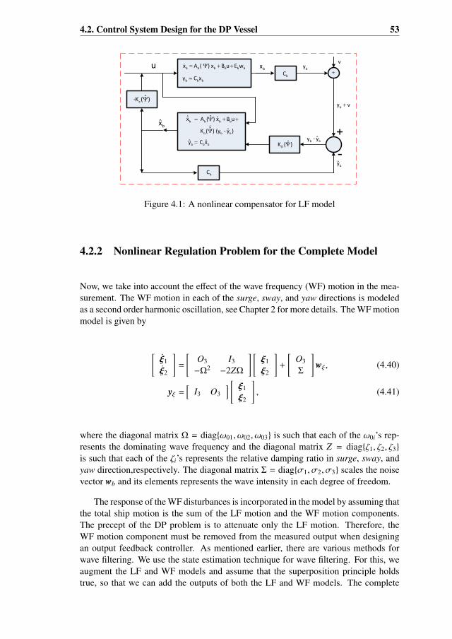
4.2. Control System Design for the DP Vessel 53
b b b b b bx A ( ) x B u E w
b b by C x
b b b bˆˆ ˆx A ( ) x B u
o b b
ˆ ˆK ( ) (y ‐ y )
b b bˆ ˆy C x ˆK ( )
cˆ‐K ( )
b bˆy ‐ y
bx
u bx
by-
bC
by v
bC
bCby
v
Figure 4.1: A nonlinear compensator for LF model
4.2.2 Nonlinear Regulation Problem for the Complete Model
Now, we take into account the effect of the wave frequency (WF) motion in the mea-surement. The WF motion in each of the surge, sway, and yaw directions is modeledas a second order harmonic oscillation, see Chapter 2 for more details. The WF motionmodel is given by
[ξ1
ξ2
]=
[O3 I3
−Ω2 −2ZΩ
] [ξ1
ξ2
]+
[O3
Σ
]wξ, (4.40)
yξ =[
I3 O3
] [ ξ1
ξ2
], (4.41)
where the diagonal matrix Ω = diagω01, ω02, ω03 is such that each of the ω0i’s rep-resents the dominating wave frequency and the diagonal matrix Z = diagζ1, ζ2, ζ3
is such that each of the ζi’s represents the relative damping ratio in surge, sway, andyaw direction,respectively. The diagonal matrix Σ = diagσ1, σ2, σ3 scales the noisevector wb and its elements represents the wave intensity in each degree of freedom.
The response of the WF disturbances is incorporated in the model by assuming thatthe total ship motion is the sum of the LF motion and the WF motion components.The precept of the DP problem is to attenuate only the LF motion. Therefore, theWF motion component must be removed from the measured output when designingan output feedback controller. As mentioned earlier, there are various methods forwave filtering. We use the state estimation technique for wave filtering. For this, weaugment the LF and WF models and assume that the superposition principle holdstrue, so that we can add the outputs of both the LF and WF models. The complete
54 Chapter 4. SDARE-based control Design
(augmented) model can be written asηνbξ1ξ2
=
O3 J(ψ) O3 O3 O3
O3 −M−1D M−1JT (ψ) O3 O3
O3 O3 −T−1 O3 O3
O3 O3 O3 O3 I3
O3 O3 O3 −Ω2 −2ZΩ
ηνbξ1ξ2
+
O3
M−1
O3
O3
O3
u
+
O3 O3
O3 O3
Ψ O3
O3 O3
O3 Σ
[
wb
wξ
], (4.42)
y =yb + yξ + v
=[
I3 O3 O3 I3 O3
]ηνbξ1
ξ2
+ v. (4.43)
The controllability matrix of (4.42) is given by
C =
O3 J(ψ)M−1 −J(ψ)M−1DM−1 · · · −J(ψ)(M−1D)13M−1
M−1 −M−1DM−1 (M−1D)2M−1 · · · (M−1D)14M−1
O3 O3 O3 · · · O3
O3 O3 O3 · · · O3
O3 O3 O3 · · · O3
,(4.44)
Since the matrices J(ψ), M, and D have full row rank for all ψ ∈ R, the controllabilitymatrix has rank 6. This means that only η and ν are controllable states while theslowly varying disturbances and wave frequency motion are not controllable. Thisis not restrictive as the objective is to control only the low frequency motion. UsingTheorem 4.1.1, a locally asymptotically stable SDARE controller for (4.42) is definedby
u = −R−1BT Πc(ψ)x
= −R−1M−1[
Π21(ψ) Π22(ψ) Π23(ψ) Π24(ψ) Π25(ψ)]ηνbξ1
ξ2
, (4.45)
where Π2i(ψ), i = 1, 2, 3, 4, 5 are obtained from the SDARE associated with (4.1) and(4.42). Again as we know that only the position measurement is available. Therefore,to realize the controller (4.45), we need estimates of the states. Then this control law
4.2. Control System Design for the DP Vessel 55
will be
u = −R−1M−1[
Π21(ψ) Π22(ψ) Π23(ψ) Π24(ψ) Π25(ψ)]ην
bξ1
ξ2
. (4.46)
Before addressing the observability of (4.42), we recall the following result from[74].
Theorem 4.2.3. Consider the system
x1 = A1x1, (4.47)
x2 = A1x2, (4.48)
y = C1x1 + C2x2, (4.49)
where x1 ∈ Rn1 and x2 ∈ R
n2 are states and y ∈ Rp is the output of the system. If A1
and A2 have no common eigenvalues, i.e.,
σ(A1) ∩ σ(A2) = φ, (4.50)
then the system (4.47)-(4.49) is observable iff (C1, A1) and (C2, A2) are both observ-able.
Proof. See [74].
The systems (4.23) and (4.40), respectively, describe the slowly varying low fre-quency and wave frequency motions with different eigenfrequencies. Therefore, thesystem matrices Ab(ψ) and Aξ in (4.23) and (4.40) do not have any common eigenval-ues. Moreover, the observability matrices (4.26) and
Oξ =
I3 O3
O3 I3...
...
(4.51)
have full row ranks. Therefore, the subsystems (Ab(ψ),Cb) and (Aξ,Cξ) of the system(4.42) are observable. This means that by Theorem 4.2.3, we can conclude that thesystem (4.42)-(4.43) is pointwise observable for all ψ ∈ R.

56 Chapter 4. SDARE-based control Design
An SDARE observer for the system (4.42)-(4.43) is defined by
˙η˙ν˙b˙ξ1˙ξ2
=
O3 J(ψ) O3 O3 O3
O3 −M−1D M−1JT (ψ) O3 O3
O3 O3 −T−1 O3 O3
O3 O3 O3 O3 I3
O3 O3 O3 −Ω2 −2ZΩ
ην
bξ1
ξ2
+
O3
M−1
O3
O3
O3
u
+ Ko(ψ)(y − y), (4.52)
y =[
I3 O3 O3 I3 O3
]ην
bξ1
ξ2
. (4.53)
The observer gain Ko(ψ) in (4.52) is given by
Ko(ψ) = Πo(ψ)CT V−1
=
Π11(ψ) + Π14(ψ)Π21(ψ) + Π24(ψ)Π31(ψ) + Π34(ψ)Π41(ψ) + Π44(ψ)Π51(ψ) + Π54(ψ)
· V−1 (4.54)
where Πi1(ψ) and Πi4(ψ), i = 1, 2, 3, 4, 5 are obtained from the solution of the dualSDARE associated with the (4.42)-(4.43).
A combination of the nonlinear controller (4.46) and the nonlinear observer (4.52)is called a nonlinear compensator and is shown in Figure 4.2. The nonlinear SDAREcompensator is given by[
x˙x
]=
[A(ψ) −BKc(ψ)
Ko(ψ)C A(ψ) − BKc(ψ) − Ko(ψ)C
] [xx
]+
[E OO Ko(ψ)
] [wv
].
(4.55)
Before concluding this section, it is important to mention that in reality, the WFmodel is considered as a disturbance to the model. For designing a control law, it isdesired that the effects of the WF disturbances do not enter into the feedback loop.In this particular example, it is required that no part of the disturbance vectors ξ1 andξ2 enters in the control action. Here, the controller gain matrix turns out to have theform, Kc(ψ) = [Kc1(ψ),Kc2(ψ),Kc3(ψ),O3,O3] which ensures the attenuation of thedisturbance; in the feedback the product term, Kc(ψ)x, eliminates ξ1 and ξ2 from thefeedback loop.
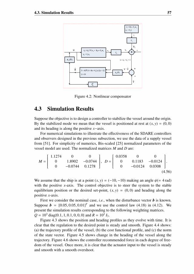
4.3. Simulation Results 57
= b b b b b bx A ( ) x B u E w
b b by C x
0ˆˆ ˆ ˆx A( ) x Bu K y y
ˆ ˆy Cx
bC
0ˆK ( )
C
cˆ‐K ( )
C
E w
y C
by y y v
ˆy ‐ yx
ubx by
y
y
+
-
v
Figure 4.2: Nonlinear compensator
4.3 Simulation ResultsSuppose the objective is to design a controller to stabilize the vessel around the origin.By the stabilized mode we mean that the vessel is positioned at rest at (x, y) = (0, 0)and its heading is along the positive x−axis.
For numerical simulations to illustrate the effectiveness of the SDARE controllersand observers designed in the previous subsection, we use the data of a supply vesselfrom [51]. For simplicity of numerics, Bis-scaled [25] normalized parameters of thevessel model are used. The normalized matrices M and D are:
M =
1.1274 0 00 1.8902 −0.07440 −0.0744 0.1278
, D =
0.0358 0 00 0.1183 −0.01240 −0.0124 0.0308
.(4.56)
We assume that the ship is at a point (x, y) = (−10,−10) making an angle ψ(= 4 rad)with the positive x-axis. The control objective is to steer the system to the stableequilibrium position or the desired set-point, (x, y) = (0, 0) and heading along thepositive x-axis.
First we consider the nominal case, i.e., when the disturbance vector b is known.Suppose b = [0.05, 0.05, 0.01]T and we use the control law (4.18) in (4.12). Wepresent the simulation results corresponding to the following weighting matrices.Q = 103 diag0.1, 1, 0.1, 0, 0, 0 and R = 102 I3.
Figure 4.3 shows the position and heading profiles as they evolve with time. It isclear that the regulation to the desired point is steady and smooth. Figure 4.4 shows:(a) the trajectory profile of the vessel, (b) the cost functional profile, and (c) the normof the state vector. Figure 4.5 shows change in the heading of the vessel along thetrajectory. Figure 4.6 shows the controller recommended force in each degree of free-dom of the vessel. Once more, it is clear that the actuator input to the vessel is steadyand smooth with a smooth overshoot.

58 Chapter 4. SDARE-based control Design
As we have already mentioned that the weighting matrices can be tuned to im-prove the performance of the controller. We elaborate this feature in the following.For instance, we penalize the velocities and take Q = 103 diag0.1, 1, 0.1, 1, 1, 1. Fig-ures 4.7 and 4.8 show the control input signals and the heading orintation of the vesselcorresponding to the new weighting matrix Q. It is clear that new profiles for theheading orientation and the control input signal are smoother than the previous pro-files. To emphasize more on tuning factor, we include another heading orientationprofile corresponding to R = 100 I3, see Figure 4.9.
0 2 4 6 8 10 12 14 16 18 20
−10
−5
0
x [m
]
(a)
0 2 4 6 8 10 12 14 16 18 20
−10
−5
0
y [m
]
(b)
0 2 4 6 8 10 12 14 16 18 20−1
0
1
2
3
4
5
Time [sec]
ψ [r
ad]
(c)
Figure 4.3: The position and heading profiles of the vessel as obtained from the closedloop system (4.12) and (4.18)
.

4.3. Simulation Results 59
−12 −10 −8 −6 −4 −2 0 2
−10
−5
0
x [m]
y [m
]
(a)
0 5 10 150
1
2
3x 10
5
Cos
t: xT
Qx+
uTR
u
(b)
0 5 10 15
0
5
10
15
Time [sec]
Nor
m: |
|x||
(c)
Figure 4.4: The evolution of the trajectory, cost, and the norm (of the state vector)profiles associated with the vessel as obtained from the closed loop system (4.12) and(4.18).
−12 −10 −8 −6 −4 −2 0 2 4−14
−12
−10
−8
−6
−4
−2
0
2
x1 [m]
Heading angle variation
x 2 [m]
Figure 4.5: The heading orientation over the trajectory of the vessel as obtained fromthe closed loop system (4.12) and (4.18).

60 Chapter 4. SDARE-based control Design
0 1 2 3 4 5 6 7 8 9 10−40
−20
0
20
40
u 1 [kN
]
(a)
0 1 2 3 4 5 6 7 8 9 10
−20
−10
0
10
20
u 2 [kN
]
(b)
0 1 2 3 4 5 6 7 8 9 10−6
−4
−2
0
2
4
Time [sec]
u 3 [kN
m]
(c)
Figure 4.6: The profiles of the individual components of the control input vector asobtained from (4.18).
−14 −12 −10 −8 −6 −4 −2 0 2 4−14
−12
−10
−8
−6
−4
−2
0
2
x1 [m]
Heading angle variation
x 2 [m]
Figure 4.7: The heading orientation over the trajectory of the vessel as obtained fromthe closed loop system (4.12) and (4.18) after changing the weighting matrices Q andR.
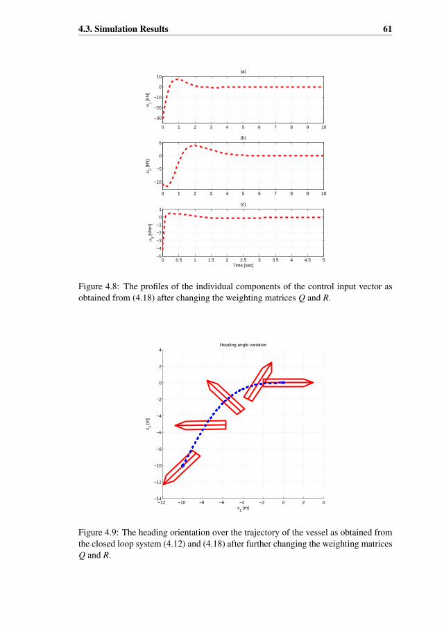
4.3. Simulation Results 61
0 1 2 3 4 5 6 7 8 9 10
−30
−20
−10
0
10
u 1 [kN
]
(a)
0 1 2 3 4 5 6 7 8 9 10
−10
−5
0
5u 2 [k
N]
(b)
0 0.5 1 1.5 2 2.5 3 3.5 4 4.5 5−5
−4
−3
−2
−1
0
1
Time [sec]
u 3 [kN
m]
(c)
Figure 4.8: The profiles of the individual components of the control input vector asobtained from (4.18) after changing the weighting matrices Q and R.
−12 −10 −8 −6 −4 −2 0 2 4−14
−12
−10
−8
−6
−4
−2
0
2
4
x1 [m]
Heading angle variation
x 2 [m]
Figure 4.9: The heading orientation over the trajectory of the vessel as obtained fromthe closed loop system (4.12) and (4.18) after further changing the weighting matricesQ and R.

62 Chapter 4. SDARE-based control Design
Next, we consider the case when the bias vector b is unknown. We consider ex-actly the same situation regarding the control objective and the initial position of thevessel, as in the nominal case. The simulation results show the performance of theSDARE-based control law and the SDARE observer to achieve the desired objective.
For the simulation results shown in the following figures, we use the bias timeconstant as T = diag100, 100, 100 while the controller weighting matrices are
Q = 10−1 diag100, 100, 10, 1, 1, 1, 0, 0, 0 and R = 10−1 diag1, 1, 0.01,
and the observer weighting matrices are
U = 100 diag1, 1, 1, 1, 1, 1, 1, 1, 10 and V = 10−2 diag1, 1, 1.
Figure 4.10 shows the measured position and heading profiles and their estimatesobtained from the SDARE observer. As desired, the profiles show a steady and smoothestimation of the noisy measurements. Figure 4.11 shows the profiles of linear velocityin surge and sway directions and the angular yaw velocity and their estimates. Figure4.12 shows the profiles of the bias estimates in surge, sway, and yaw directions. Figure4.13 shows: (a) the trajectory profile, (b) the cost functional profile, and (c) the normof the state vector and its estimate. Figure 4.14 shows the heading orientation with thetrajectory. The profile shows a smooth and steady path and orientation of the vessel.Figure 4.15 shows the control input signals from the controller in each degree of free-dom. The profiles show that the controller adjusts in the start and then signals becomesteady and smooth. From all these figures, we see that the SDARE compensator statesshow nice asymptotic convergence to the desired point.
To emphasize the role of the weighting matrices, we include some more simula-tions. For instance, we take
Q = 10−2 diag100, 100, 10, 1, 1, 1, 0, 0, 0 and R = 10−3 diag1, 1, 0.01.
This means that we reduce the penalty on both the vectors x and u. Figures 4.16 and4.17 show the corresponding profiles of the trajectory and the control input signals.The vessel takes a relatively longer route but its smoother than the one we obtainedwith the previous weighting matrices. The control input signals are also amplified asexpected.
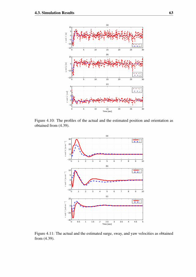
4.3. Simulation Results 63
0 5 10 15 20 25 30−15
−10
−5
0
5
10
xandx[m
]
(a)
xx
0 5 10 15 20 25 30−20
−10
0
10
yandy[m
]
(b)
yy
0 5 10 15 20 25 30
−2
0
2
4
6
ψandψ
[rad]
Time [sec]
(c)
ψ
ψ
Figure 4.10: The profiles of the actual and the estimated position and orientation asobtained from (4.39).
0 1 2 3 4 5 6 7 8 9 10−10
0
10
20
30
uandu[m
-sec
−1]
(a)
uu
0 1 2 3 4 5 6 7 8 9 10−10
−5
0
5
10
vandv[m
-sec
−1]
(b)
vv
0 0.5 1 1.5 2 2.5 3 3.5 4 4.5 5−40
−20
0
20
randr[rad-sec
−1]
(c)
Time [sec]
rr
Figure 4.11: The actual and the estimated surge, sway, and yaw velocities as obtainedfrom (4.39).

64 Chapter 4. SDARE-based control Design
0 5 10 15−10
−8
−6
−4
−2
0
2
b 1[kN]
(a)
0 5 10 15
−10
−5
0
b 2[kN]
(b)
0 5 10 15
−2
0
2
4
6
b 3[kN-m
]
(c)
Time [Sec]
Figure 4.12: The bias estimates in surge, sway, and yaw directions as obtained from(4.39).
−12 −10 −8 −6 −4 −2 0 2 4 6−15
−10
−5
0
5
x [m]
y [m
]
xy−trajectory
0 1 2 3 4 5 6 7 8 9 100
1000
2000
3000
4000
Cost:xTQx+uTRu
(b)
0 5 10 15 20 25 300
10
20
30
40
Time [sec]
||x||and||x
||
(c)
||x||||x||
Figure 4.13: The trajectory and the profiles of the cost functional and the norms of themeasured state and its estimate as obtained from (4.39).

4.3. Simulation Results 65
−14 −12 −10 −8 −6 −4 −2 0 2 4 6−16
−14
−12
−10
−8
−6
−4
−2
0
2
4
x1 [m]
Heading angle variation
x 2 [m]
Figure 4.14: The heading orientation along the trajectory as obtained from (4.39).
0 1 2 3 4 5 6 7 8 9 10−50
0
50
100
150
u 1 [kN
]
(a)
0 1 2 3 4 5 6 7 8 9 10
−100
0
100
u 2 [kN
]
(b)
0 0.2 0.4 0.6 0.8 1 1.2 1.4 1.6 1.8 2
−50
0
50
Time [sec]
u 3 [kN
−m
]
Figure 4.15: The control input signals for each degree of freedom as computed from(4.30).
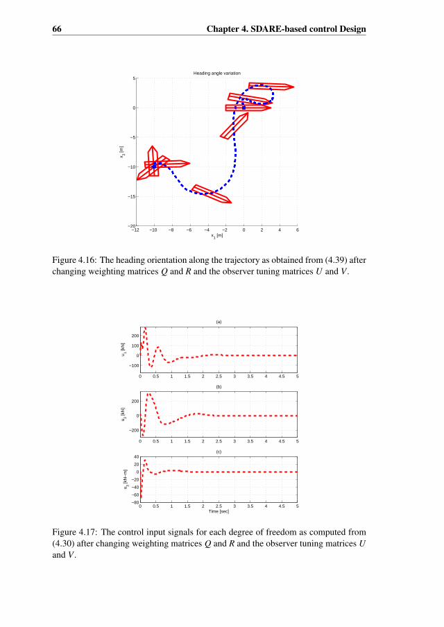
66 Chapter 4. SDARE-based control Design
−12 −10 −8 −6 −4 −2 0 2 4 6−20
−15
−10
−5
0
5
x1 [m]
Heading angle variation
x 2 [m]
Figure 4.16: The heading orientation along the trajectory as obtained from (4.39) afterchanging weighting matrices Q and R and the observer tuning matrices U and V .
0 0.5 1 1.5 2 2.5 3 3.5 4 4.5 5
−100
0
100
200
u 1 [kN
]
(a)
0 0.5 1 1.5 2 2.5 3 3.5 4 4.5 5
−200
0
200
u 2 [kN
]
(b)
0 0.5 1 1.5 2 2.5 3 3.5 4 4.5 5−80
−60
−40
−20
0
20
40
Time [sec]
u 3 [kN
−m
]
(c)
Figure 4.17: The control input signals for each degree of freedom as computed from(4.30) after changing weighting matrices Q and R and the observer tuning matrices Uand V .

4.3. Simulation Results 67
Finally, we consider the case when the WF motion is also playing a role. For thesimulation results shown in the following figures, we use the bias time constant asT = diag100, 100, 100, the dominating wave frequencies as Ω = diag0.9, 0.9, 0.9,the relative damping ratios as Z = diag0.2, 0.2, 0.2, the controller weighting matricesas
Q = 10−1 diag100, 100, 10, 1, 1, 1,O1×9, and R = 10−1 diag1, 1, 0.01
and the observer weighting matrices as
U = 100 diag1, 1, 1, 1, 1, 1, 1, 1, 10, 1, 1, 1, 1, 1, 1 and V = 10−1 diag1, 1, 1.
Figure 4.18 shows the profiles of the measured position and heading, and their es-timates obtained from the SDARE observer. The profiles depict a smooth and steadyregulation of the vessel to the desired position. Figure 4.19 shows the velocity pro-files of the vessel motion and their estimates along surge, sway, and yaw directions.Figure 4.20 shows the bias estimates obtained from the SDARE observer. Figure 4.21shows: (a) the trajectory of the vessel motion, (b) the cost functional profile, and (c)the norm of the measured state vector and its estimate. In Figure 4.22, we show theheading orientation along the trajectory. The traectory and orientation are nice andsmooth. Figure 4.23 shows the control input signal in each degree of freedom com-puted from (4.46). As in the previous case, the control signals need some adjustmentin the beginning and then become smooth and steady.
To further elaborate the importance of the weighting matrices, we add some moresimulation results. Now, Lets take the matrices
Q = 10−2 diag100, 100, 10, 1, 1, 1,O1×9 and R = 10−3 diag1, 1, 0.01.
Figures 4.24 and 4.25 show the corresponding trajectory and control input signals.It can be seen that the vessel follows a relatively longer path but its slightly betterthan the previous path. The control input signals are amplified with this choice of thetuning matrices.
Further lets modify the observer weighting matrix U: we now take
U = 100 diag10, 10, 10, 1, 1, 1, 1, 1, 10, 1, 1, 1, 1, 1, 1.
Figures 4.26 and 4.27 show the corresponding profiles of the trajectory and the controlinput signals. The trajectory profile has further improved and control input profilesshow an increased control input.

68 Chapter 4. SDARE-based control Design
0 5 10 15 20 25 30−20
−10
0
10
xandx[m
]
(a)
xx
0 5 10 15 20 25 30−20
−10
0
10yandy[m
](b)
yy
0 5 10 15 20 25 30−5
0
5
ψandψ
[rad]
Time [sec]
(c)
ψ
ψ
Figure 4.18: The position and heading profiles of the vessel motion as obtained fromthe compensator (4.55).
0 1 2 3 4 5 6 7 8 9 10−10
0
10
20
uandu[m
-sec
−1]
(a)
uu
0 1 2 3 4 5 6 7 8 9 10−10
−5
0
5
10
vandv[m
-sec
−1]
(b)
vv
0 0.5 1 1.5 2 2.5 3 3.5 4 4.5 5−40
−20
0
20
randr[rad-sec
−1]
Time [sec]
(c)
rr
Figure 4.19: The velocities and their estimates along surge, sway, and yaw directionsas obtained from (4.55).
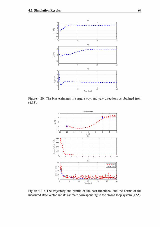
4.3. Simulation Results 69
0 5 10 15−10
−8
−6
−4
−2
0
2
b 1[kN]
(a)
0 5 10 15
−10
−5
0
b 2[kN]
(b)
0 5 10 15
−2
0
2
4
6
b 3[kN-m
]
(c)
Time [Sec]
Figure 4.20: The bias estimates in surge, sway, and yaw directions as obtained from(4.55).
−12 −10 −8 −6 −4 −2 0 2 4−15
−10
−5
0
5
x [m]
y [m
]
xy−trajectory
0 1 2 3 4 5 6 7 8 9 100
1000
2000
3000
4000
Cost:xTQx+uTRu
(b)
0 5 10 15 20 25 300
10
20
30
40
Time [sec]
||x||and||x
||
(c)
||x||||x||
Figure 4.21: The trajectory and profile of the cost functional and the norms of themeasured state vector and its estimate corresponding to the closed loop system (4.55).

70 Chapter 4. SDARE-based control Design
−14 −12 −10 −8 −6 −4 −2 0 2 4 6−14
−12
−10
−8
−6
−4
−2
0
2
4
x1 [m]
Heading angle variation
x 2 [m]
Figure 4.22: The heading orientation along the trajectory as obtained from (4.55).
0 1 2 3 4 5 6 7 8 9 10−50
0
50
100
150
u 1 [kN
]
(a)
0 1 2 3 4 5 6 7 8 9 10
−100
0
100
u 2 [kN
]
(b)
0 0.2 0.4 0.6 0.8 1 1.2 1.4 1.6 1.8 2−100
−50
0
50
Time [sec]
u 3 [kN
−m
]
Figure 4.23: The control input signals for each degree of freedom as obtained from(4.46).
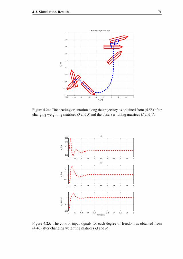
4.3. Simulation Results 71
−12 −10 −8 −6 −4 −2 0 2 4 6−14
−12
−10
−8
−6
−4
−2
0
2
4
x1 [m]
Heading angle variation
x 2 [m]
Figure 4.24: The heading orientation along the trajectory as obtained from (4.55) afterchanging weighting matrices Q and R and the observer tuning matrices U and V .
0 0.5 1 1.5 2 2.5 3 3.5 4 4.5 5
−100
0
100
200
300
u 1 [kN
]
(a)
0 0.5 1 1.5 2 2.5 3 3.5 4 4.5 5
−200
0
200
u 2 [kN
]
(b)
0 0.2 0.4 0.6 0.8 1 1.2 1.4 1.6 1.8 2−100
−50
0
Time [sec]
u 3 [kN
−m
]
Figure 4.25: The control input signals for each degree of freedom as obtained from(4.46) after changing weighting matrices Q and R.
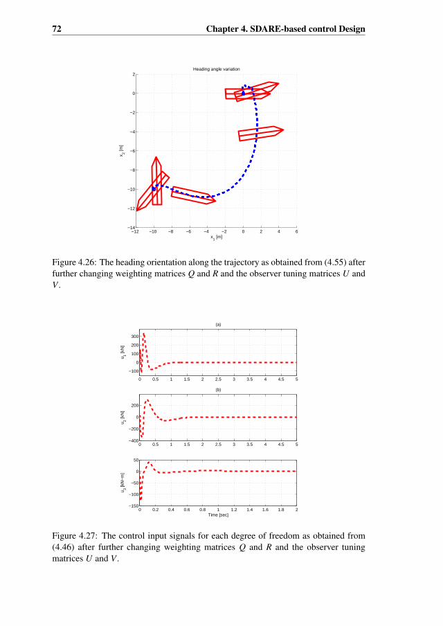
72 Chapter 4. SDARE-based control Design
−12 −10 −8 −6 −4 −2 0 2 4 6−14
−12
−10
−8
−6
−4
−2
0
2
x1 [m]
Heading angle variation
x 2 [m]
Figure 4.26: The heading orientation along the trajectory as obtained from (4.55) afterfurther changing weighting matrices Q and R and the observer tuning matrices U andV .
0 0.5 1 1.5 2 2.5 3 3.5 4 4.5 5
−100
0
100
200
300
u 1 [kN
]
(a)
0 0.5 1 1.5 2 2.5 3 3.5 4 4.5 5−400
−200
0
200
u 2 [kN
]
(b)
0 0.2 0.4 0.6 0.8 1 1.2 1.4 1.6 1.8 2−150
−100
−50
0
50
Time [sec]
u 3 [kN
−m
]
Figure 4.27: The control input signals for each degree of freedom as obtained from(4.46) after further changing weighting matrices Q and R and the observer tuningmatrices U and V .
4.4. Conclusions 73
4.4 ConclusionsWe study the regulation problem of a DP vessel by using the SDARE technique.We extend the concept of the LQR problem to nonlinear system by using the SDCparametrization. This gives rise to an SDARE which must be solved to obtain a sub-optimal solution of the nonlinear regulation problem.
The DP vessel model shows that only the position and heading measurementsare available from the sensors. This is an inadequate information for the SDAREcontrol design problem which requires complete state knowledge. Using the stabi-lizability and detectability of the vessel model together with the duality concept, wepropose a suboptimal locally asymptotically stable SDARE observer. The combina-tion of the locally asymptotically stable SDARE regulator and SDARE observer is alocally asymptotically stable SDARE compensator.
We divide the study of the DP vessel regulation problem in two steps. First, westudy the LF motion regulation without taking into account the WF motions. We beginby considering a nominal case (the bias disturbance vector is known or its estimate isavailable) and come up with a PD-type control law with a feedforward term. Thecontroller is proved to be globally asymptotically stable by using the LMIs and theLyapunov stability theory.
Afterwards, we assume that the bias vector is unknown and the measured signalsfrom the sensors are contaminated by noise. We combine the concept of the SDAREregulation and estimation (to estimate the position, velocity, and bias vectors) to comeup with a locally asymptotically stable SDARE compensator. Second, we take intoaccount both the LF and WF motions and use again the SDARE method to address theregulation and estimation problems. A locally asymptotically stable compensator isobtained by combining locally asymptotically stable controller and estimator. We usethe data of a supply vessel for simulation experiments. Simulation results presented inthis chapter confirm the asymptotic stability of the SDARE regulator and the SDAREestimator.

74
Chapter 5The Fourier Series InterpolationMethod1
In Chapter 4, the controller and observer gains are state dependent. They are requiredto be determined by online solving the concerned SDAREs. These SDAREs have aspecial form in which the coefficient matrix depends on a single state component in aperiodic way. In this chapter, we propose a new method for solving these SDAREs.This method is based on the Fourier series. This method reduces the online compu-tation time for the solution of these SDAREs by performing the major computationaltask offline.
The earliest traces of the use of the algebraic Riccati equation in control relatedproblems can be found in the works on the solution of the LQ optimal control andfiltering problem [41] and on approximation methods in optimal control [67]. To dateits scope has been extended to address problems of nonlinear state regulation andestimation, estimator based feedback control synthesis, H∞−control, H2−control, andnonlinear filter design, for instance see [7], [14], [31], [52], and [66]. Recently, thestate dependent Riccati equation based technique has been used in nonlinear optimalvehicle control in [2].
The SDARE has emerged in many practical applications. Especially, the SDAREhas become an important research topic in ongoing developments in the areas of con-trol and estimation theory. It has been regarded as an efficient tool to tackle problemsrelated with the nonlinear control design, filtering, synthesis, and analysis. Conse-quently, emphasis has been put on developing computationally efficient solution meth-ods for the SDARE.
In a broader perspective, we divide the solution methods in two categories: itera-tive and direct. Both type of methods have positive and negative features. Mainly, thedirect methods are computationally faster than the iterative methods, especially whenthe problem is poorly conditioned or when a good-quality initial guess is not available.
1This work has been published in the proceedings of the UKACC International Conference on Control(CONTROL 2010), see [57].
75
76 Chapter 5. The Fourier Series Interpolation Method
On the other hand, the direct methods require more storage capacity than the iterativemethods. Some of the well-known direct methods are the Taylor series method [7],the generalized eigenvector approach [15], the matrix sign function method [17], theinformation filter algorithm [39], and the Schur decomposition method [49]. Someof the well-known iterative methods are the Kleinman algorithm [3], the interpolationmethods [7], the Newton-method and its modified forms [9, 18, 40], solution via spec-tral factorization, the doubling algorithm [13, 44], and the Chandrasekhar algorithm[72].
In (4.5), we observe that the controller gain is not fixed but it varies with thestate of the system. The computation of the controller gain requires the solution of theSDARE (4.6). Therefore, in the feedback loop, the controller gain is computed online.As pointed out in [12] the reduction in the online computation time of the solution ofthe SDARE is a major issue because of its high computational cost. In this chapter, wepropose the Fourier series based numerical method for the solution of the SDARE oftype (4.7) which reduces the online computations. Henceforth, we call this method theFourier series interpolation (FSI) method. This method of solution is computationallyvery simple and hence, it is valuable in the situations where online computation of thesolution of the SDARE is required.
5.1 The Fourier Series Interpolation (FSI) MethodFirst we explain why it is reasonable to use the Fourier series for the solution of thealgebraic Riccati equations of the type (4.7). Then we will illustrate the details of theFSI method. For a general formulation of the FSI method, we make a slight change ofnotation in the SDARE (4.7). We consider the following form
Π(x1)A(x1) + AT (x1)Π(x1) + Q − Π(x1)BR−1BT Π(x1) = 0, (5.1)
where x1 ∈ R, without loss of generality, is the first component of the state vectorx ∈ Rn, A(·) ∈ Rn×n is a C∞ function2, Π(·) ∈ Rn×n, and B ∈ Rn×m.
The matrix function A(·) is smooth and θ−periodic, i.e., A(x1) = A(x1 + θ) for allx1 ∈ R. The solution matrix Π(·), provided it exists, is also a smooth and θ−periodicfunction, see [16]. At this point, we recall two important results from [35] whichendorse the idea of using the Fourier series for finding an approximate solution of theSDARE (5.1). First, we recall the Fourier convergence theorem due to Dirichlet.
Theorem 5.1.1. (The Fourier Convergence Theorem) Let f be a piecewise smoothfunction on the interval −L ≤ x ≤ L, then the Fourier series of f converges1. to f (x), if f is continuous at x ∈ (−L, L).2. to the average of the two limits,
12
[ f (x+) + f (x−)],
if f has a jump discontinuity at x ∈ (−L, L), where f (x−) and f (x+) means, respec-tively, the left and the right hand limits of the function f at point x.
2C∞(R,Rn×m) := A : R −→ Rn×m | A is Ck for all k ≥ 0.
5.1. The Fourier Series Interpolation (FSI) Method 77
The periodic extension of a 2L−periodic function is always admissible. The fol-lowing corollary gives the necessary and sufficient condition for the continuity of theperiodic extension of a piecewise smooth function.
Corollary 5.1.1. For a 2L−periodic piecewise smooth function f , the periodic exten-sion of f is continuous for all x ∈ R if and only if f is continuous and f (−L) = f (L).
In the context of the vessel model, the solution Πc(ψ) of the SDARE (4.7) is asmooth matrix function with period θ. Therefore, by the above results, it is possible torepresent the matrix function Π(·) in the form of a Fourier series. This means that theFourier series of Π(·) exists and converges to Π(x1) for all x1 ∈ R. Thus we write
Π(x1) =A0
2+
∞∑k=1
(Ak cos
(2kπx1
θ
)+ Bk sin
(2kπx1
θ
)). (5.2)
The Fourier coefficients A0, Ak ∈ Rn×n and Bk ∈ R
n×n for k = 1, 2, 3, ..., are defined by
Ak =2θ
∫ θ2
− θ2
Π(x1) cos(
2kπx1
θ
)dx1, k = 0, 1, 2, 3, .... (5.3)
and
Bk =2θ
∫ θ2
− θ2
Π(x1) sin(
2kπx1
θ
)dx1, k = 1, 2, 3, .... (5.4)
Let us now recall a well-known result by Riemann and Lebesgue which is statedin the following lemma.
Lemma 5.1.1. (The Riemann-Lebesgue Lemma) If f is an integrable function on[− θ2 ,
θ2 ] then
limk→∞
∫ θ2
− θ2
f (x) sin kx dx = 0,
and
limk→∞
∫ θ2
− θ2
f (x) cos kx dx = 0,
From the fact that the series on the right hand side of (5.2) is convergent andfrom the statement of the Lemma 5.1.1, it follows that the Fourier coefficients withsufficiently high indices are negligibly small (their norms are of order zero) and canbe left out. Therefore, for any small positive number ε, there exists an integer N′ suchthat ||An||2 < ε and ||Bn||2 < ε, ∀n > N′. We use the spectral matrix norm in thischapter.
We explain the procedure to compute the Fourier coefficients as follows. First, wedecide a stopping criterion for the computation of the Fourier coefficients. We definea tolerance level say ε′ > 0, such that the process of the computation of the Fourierseries coefficients stops when∥∥∥∥∥∥∥Π(x1) −
A0
2+
N∑k=1
(Ak cos
(2kπx1
θ
)+ Bk sin
(2kπx1
θ
))∥∥∥∥∥∥∥
2
< ε′, (5.5)
78 Chapter 5. The Fourier Series Interpolation Method
is satisfied for all x1 ∈ [− θ2 ,θ2 ).
Then, we start with N = 1 such that there are 2N +1(= 3) Fourier coefficients to bedetermined. Equation (5.2) holds identically true for all x1 ∈ [− θ2 ,
θ2 ). Take m > 2N+1
points x1t ∈ [− θ2 ,θ2 ), t = 1, 2, ...,m. To each point x1t ∈ [− θ2 ,
θ2 ), there corresponds an
equation of the following form
A0
2+
N∑k=1
(Ak cos
(2kπx1t
θ
)+ Bk sin
(2kπx1t
θ
))= Π(x1t ). (5.6)
In this way, we get the following nonhomogeneous system of m linear matrix equa-tions
12 cos
2πx11θ · · · cos
2Nπx11θ sin
2πx11θ · · · sin
2Nπx11θ
12 cos
2πx12θ · · · cos
2Nπx12θ sin
2πx12θ · · · sin
2Nπx12θ
.
.
....
.
.
....
.
.
....
.
.
.12 cos 2πx1m
θ · · · cos 2Nπx1mθ sin 2πx1m
θ · · · sin 2Nπx1mθ
A0A1...
ANB1...
BN
=
Π1Π2...
Πm
,
where Πi = Π(x1i ). We can write this in short form as
AX = B (5.7)
However, note that the dimensions of the matrices in (5.7) do not conform withthe usual matrix multiplication rules. We use the Kronecker matrix product to removethis discrepancy. For this we multiply the matrixA from right by In in the Kroneckersense. This results in
(A⊗ In)X = B. (5.8)
The equation (5.8) can be solved in the least-squares sense, minimize∥∥∥∥(A⊗In)X−B
∥∥∥∥2.
The solution X to this problem yields 2N + 1 Fourier coefficients. The Fourier seriesapproximation of the solution of the SDARE (5.1) is then given by
Π(x1) ≈A0
2+
N∑k=1
(Ak cos
(2kπx1
θ
)+ Bk sin
(2kπx1
θ
)). (5.9)
Now the stopping criterion (5.5) is tested. This can be done by plotting ε′ − g(x1)vs x1 on the interval [− θ2 ,
θ2 ), where g(x1) is the LHS of (5.5). To get a smooth sketch,
we take enough points on the interval. This will also ensure that we did not overlookany sharp peaks or discontinuities. If the stopping criterion is satisfied (plot lies abovex1-axis) then we stop. Otherwise, we repeat the above procedure for the next integervalue of N(= 2) and so on, and continue until the stopping criterion is satisfied. The
5.2. Performance Analysis 79
algorithm for finding the Fourier coefficients is summarized below3.
Algorithm 5.1.1: Computation of the Fourier Coefficients (FCs)
input: The tolerance parameter ε′ and an integer N(= 1).
assumption: The m number of interpolation points must satisfy m > 2N + 1.
output: The Fourier Coefficients A0, A1, A2, ..., AN , B1, B2, ..., BN .
for N ← 1 to some f inite large natural numberstep 1: Take m > 2N + 1.
step 2: Take xti ∈ [− θ2 ,θ2 ), i = 1, 2, 3, ...m.
step 3: Solve (5.1) at m interpolation points to get Π1,Π2, ...,Πm. (i)
step 4: Use statement (i) of this algorithm and (5.6) to get (5.7).
step 5:
Use Kronecker matrix product to get a linear system ofequations (5.8).
step 6:
Solve the linear system (5.8) to get the desired Fouriercoefficients.
if the tolerance condition is satis f ied
then
Fourier Coe f f icients A[0], A[1], ..., A[N], B[1], B[2], ...., B[N]are obtained.
elsecontinue the f or loop until tolerance condition is satis f ied.
The main step of the algorithm is step 6 of the for loop. The repetition of the loopcontinues until the stopping criteria is satisfied. We conclude this section with thefollowing remark about the above algorithm.
Remark 5.1.1. We take the number m of distict points in [− θ2 ,θ2 ), greater than the
number of Fourier coefficients 2N+1 to be determined to generate an over-determinedsystem of linear equations. The system (5.8) has a solution because rank(A ⊗ In) =
rank(A⊗ In,B).
5.2 Performance Analysis
In this section we explain why the FSI method is effectively a better method for onlinecomputation of the solution of the SDARE than “care” in terms of computation time.We do so on the basis of flop count. Equations (4.20), (4.39) and (4.55) describe thefeedback dynamics of the SDARE nonlinear compensator. The presence of Kc(ψ) andKo(ψ) therein indicates that two SDAREs have to be solved at each iteration whenthe ode systems (4.20), (4.39) and (4.55) are solved numerically. This demands acomputationally efficient method for finding the solution of the SDARE.
3The author is thankful to Professor Donald Kreher for his help on the pseudocode environment.

80 Chapter 5. The Fourier Series Interpolation Method
We compare the FSI method with the Schur decomposition method [15]. TheMATLAB routine “care” is based on this method. For each ψ, the SDARE (4.7)reduces to a continuous time algebraic Riccati equation (CARE)
ΠA + AT Π + Q − ΠBR−1BT Π = 0, (5.10)
We solve the closed loop system equations by using the MATLAB solver ode45. Dur-ing the process of computation of the numerical solution of the closed loop system,MATLAB routine “care” is called multiple times to solve (5.10). In the following weexplain some details of the Schur decomposition method for a better understanding ofthe computational complexity of this method.
The Schur decomposition method requires two major computations for solving theSDARE. First step is the reduction of the Hamiltonian matrix to an ordered real Schurform (RSF). The Hamiltonian matrix associated with (5.10) is given by
H =
[A −BR−1BT
−Q −AT
]. (5.11)
The following result ensures that the Hamiltonian matrix (5.11) does not have anyeigenvalue on the imaginary axis.
Theorem 5.2.1. (Relationship between the Hamiltonian Matrix and the RiccatiEquations) Let (A,B) be stabilizable and (A,Q) be detectable. Then the HamiltonianmatrixH has n eigenvalues with negative real parts, no eigenvalues on the imaginaryaxis, and n eigenvalues with positive real parts. In this case the CARE (5.10) has aunique stabilizing solution Π.
Now using the QR-factorization, H can be transformed into RSF form accordingto the following result.
Theorem 5.2.2. (The Real Schur Triangularization Theorem) LetH be a 2n × 2nHamiltonian matrix. Then there exists a 2n × 2n matrix Qrs such that
QTrsHQrs = Rrs =
R11 R12 · · · R1k
0 R22 · · · R2k...
......
...
0 0 0 Rkk
, (5.12)
where each Rii is either a scalar or a 2 × 2 matrix. The scalar diagonal entries corre-spond to real eigenvalues, and each 2×2 matrix on the diagonal has a pair of complexconjugate eigenvalues. The matrix Rrs is known as the RSF ofH .
The eigenvalues in (5.12) are not ordered so an additional step is made to get anordered RSF which is important for the next step which uses the invariant subspace ofthe stable eigenvalues of H to solve (5.10). The following definition and subsequenttheorem and corollary summarize the concluding step of the Schur decompositionmethod.

5.2. Performance Analysis 81
Definition 5.2.1. (Basis of an Invariant Subspace from RSF) Let
QTrsHQrs = Rrs =
[R11 R12
0 R22
], (5.13)
and let us assume that eigenvalues of R11 and R22 respectively are the negative andpositive eigenvalues of the Hamiltonian matrix H . Then the first p columns of Qrs,where p is the order of R11, form an orthonormal basis for the invariant subspaceassociated with the stable eigenvalues ofH .
Theorem 5.2.3. A matrix Π is a solution of the CARE (5.10) if and only if the columns
of(
IΠ
)span an n-dimensional invariant subspace of the Hamiltonian matrixH .
Corollary 5.2.1. If the columns of(
Π1
Π2
)span an n-dimensional invariant subspace
of the Hamiltonian matrix H associated with the CARE (5.10) and Π1 is invertible,then Π = Π2Π−1
1 is a solution of the CARE (5.10).
The Schur method is based on reduction of the Hamiltonian matrix H to RSFwhich is done by QR factorization. The exact flop count is not possible as QR-factorization is an iterative procedure. However, by the empirical observations it isassumed that on average each eigenvalue requires 2 QR-factorizations, [15]. The QR-factorization of a matrix requires O(n3) flops which means that the RSF obtained inthe first step of the Schur decomposition method also requires O(n3) flops. The order-ing of the eigenvalues in RSF requires O(n) flops. In the second step, the computationof Π = Π2Π−1
1 is done by using the least-squares algorithm and this also requiresO(n3) flops. Therefore the Schur decomposition requires O(n3) flops each time CARE(5.10) is solved online. On the other hand, the FSI method requires simple matrixaddition (O(n2) flops) and scalar-matrix multiplication (O(n2) flops). Therefore, theFSI method requires O(n2) flops when the online solution of (5.10) is computed bythis method.
The computationally expensive task in FSI method is the computation of the Fouri-er coefficients which is done offline, only once. From the algorithm given in Section5.1, we see that the computation of the Fourier coefficients involve two major steps.First, the computation of the solution of the SDARE at a known (m) number of points.Second, the solution of a linear system of equations. Each requires O(n3) flops.
Based on the foregoing discussion, we conclude that the FSI method reduces theonline computations in a feedback dynamics based on an SDARE control law. InTable 5.1, by using the simulation results discussed in Section 4.3, we quantitativelydemonstrate that the FSI method reduces the online computation time for the solutionof the SDARE. Each of the closed loop systems (4.20), (4.39) and (4.55) are solvedwith the MATLAB routine ode45 on a time interval [0, 30]. Table 5.1 shows a com-parison between the computer time required to solve the closed loop systems with theFSI method and by the MATLAB routine “care”. We notice that with the increase inthe size of the system, the performance of the FSI method is still comparable to itsperformance with a lower order system. The simulations have been performed on anIntel Centrino duo running at the frequency of 2 GHz having 2 GB RAM.
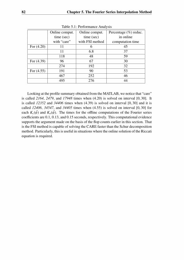
82 Chapter 5. The Fourier Series Interpolation Method
Table 5.1: Performance AnalysisOnline comput. Online comput. Percentage (%) reduc.
time (sec) time (sec) in onlinewith “care” with FSI method computation time
For (4.20) 11 6 4511 6.8 37
118 48 59For (4.39) 96 67 30
274 192 32For (4.55) 191 90 53
467 252 46495 276 44
Looking at the profile summary obtained from the MATLAB, we notice that “care”is called 2164, 2479, and 17948 times when (4.20) is solved on interval [0, 30]. Itis called 12352 and 34406 times when (4.39) is solved on interval [0, 30] and it iscalled 12406, 34547, and 34405 times when (4.55) is solved on interval [0, 30] foreach Kc(ψ) and Ko(ψ). The times for the offline computations of the Fourier seriescoefficients are 0.1, 0.13, and 0.15 seconds, respectively. This computational evidencesupports the argument made on the basis of the flop counts earlier in this section. Thatis the FSI method is capable of solving the CARE faster than the Schur decompositionmethod. Particularly, this is useful in situations where the online solution of the Riccatiequation is required.
Chapter 6Port-Hamiltonian Formulationand Passivity Based ControlDesign1
This chapter focuses on the design of the control law for dynamic positioning as-suming that the filtering and estimation problems have been solved, i.e., the
measured output contains only the noise free LF position and heading measurementsand the disturbances vector is either known or its estimate is available. The Port-Hamiltonian framework is a very useful concept which offers more capacity to im-prove the performance of the controllers and to analyze stability properties. Passivity-based techniques were first introduced in [38], [53], and [87] in the early 1970’s. Thesetechniques have been used since then in many applications, for instance in underwatervehicles [4], the control of electrical machines [21], the design of power system stabi-lizers [61], adaptive control for rigid robots [63], underactuated mechanical systems[64], power converters [69], and magnetic levitation systems [70].
A nice feature of the passivity-based control design is the physical meaning of theresulting control laws and concepts, such as storage energy or dissipation, which playa fundamental role in analyzing stability and the performance of the controller. Sta-bility properties, based on the Lyapunov theory, can easily be studied for the closedloop systems obtained. The passivity based approach has two versions. The classicalEuler Lagrange (EL-PBC) allows the change in the potential energy function and thegeneralized inertia matrix, see [65]. In the last decade, the Interconnection and Damp-ing Assignment Passivity Based Control (IDA-PBC) methodology has emerged as aneasy and a (quasi) step-by-step methodology to obtain passivity based controllers, seefor instance [65]. IDA-PBC also allows changes in the interconnection matrix.
This chapter introduces the port-Hamiltonian model of a vessel with 3 degreesof freedom in a horizontal plane. The obtained port-Hamiltonian equations are the
1This work has been published in the proceedings of the Dynamic Positioning Conference DP2010 inHouston, see [55]. It is also to appear at the IET Journal of Control Theory and Applications, see [56].
83

84 Chapter 6. pH Formulation and PBC Design
starting point for the design of controllers using the IDA-PBC technique. The maincontribution of this chapter is a family of passivity-based controllers, in the port-Hamiltonian framework, which uses the energy shaping of the closed loop systemto ensure (local/global) asymptotic stability. The resulting control laws are of output-feedback form and are robust in presence of eventual disturbances.
6.1 Hamiltonian-Based Control
6.1.1 Port-Hamiltonian ModelingA large class of physical systems of interest in control applications can be modeledin the general form of port-Hamiltonian systems (PHS), see [84]. PHS generalizethe Hamiltonian formalism of classical mechanics to physical systems connected ina power-preserving way and encodes the detailed energy transfer and storage in thesystems, and is thus suitable for control schemes based on IDA-PBC.
A PHS can be written, in an implicit form, as
x = (J(x) − R(x))∂H(x) + G(x)u, (6.1)
where x ∈ Rn is the state (or Hamiltonian variables) vector, J(x) ∈ Rn×n is the skew-symmetric interconnection matrix (J = −JT ), R(x) ∈ Rn×n is the dissipation (ordamping) matrix (symmetric positive semi-definite, R = RT ≥ 0), G(x) ∈ Rn×m isthe external connection matrix, u ∈ Rm is the control input vector, and H(x) is theHamiltonian (energy or storage) function2. In this formulation, the matrix R describesthe energy losses of the system, the interconnection matrix J describes the flow ofenergy inside the system, and the port matrix G describes the flow of energy fromoutside (for instance from the controller) to the system. In a passivity based controldesign approach, the controller can be considered as a source injecting energy into thesystem.
The so-called passive output, y ∈ Rm, is given by
y = GT (x)∂H(x), (6.2)
and the product uT y usually has unity of power. In the literature on port-Hamiltoniansystems, the so-called passive output is a relative degree one output.
6.1.2 The IDA-PBC TechniqueThe Interconnection and Damping Assignment Passivity Based Control (IDA-PBC),[65], is a technique for designing controllers based on the port-Hamiltonian frame-work. It uses the passive stability properties to ensure the convergence of the systemto the desired fixed point.
The main idea behind the IDA-PBC is to define a new closed loop (or target)system with a Hamiltonian structure. The design problem summarizes into finding a
2The ∂x (or ∂, if no confusion arises) operator defines the gradient of a function of x, and in what followswe will take it as a column vector.

6.1. Hamiltonian-Based Control 85
control law such that the system behaves as
x = (Jd − Rd)∂Hd, (6.3)
where Jd(x) = −JTd (x), Rd(x) = RT
d (x) ≥ 0 and Hd(x) has a minimum at the desiredregulation point xd, xd = arg min(Hd(x)). The stability of this system can easily beproved by using Hd as a Lyapunov function (Hd(x) = − (∂Hd)T
Rd∂Hd ≤ 0, see forinstance, [62] and [65] for a detailed discussion).
The design procedure reduces to finding matrices Jd(x) and Rd(x) and a desiredclosed loop energy function Hd(x), which solve the so-called matching equation
(J − R)∂H + Gu = (Jd − Rd)∂Hd. (6.4)
Then, the control law becomes
u =(GT G
)−1GT ((Jd − Rd)∂Hd − (J − R)∂H) . (6.5)
A drawback of the IDA-PBC controllers is that they are, in general, not able toreject disturbances. To remove this discrepancy of the control design, usually a dy-namic extension of the system is introduced to obtain an integral action on the outputerror. Extension of the closed loop dynamics in the IDA-PBC framework can be done,in a natural way, only for passive outputs, see [62]. A completely different approachaddresses non-passive outputs (or higher relative degree one outputs). In this case, aHamiltonian based controller with an integral action can be obtained via a change ofvariables, see [20].
Let us assume that the xo ∈ Rr are the higher relative degree one (or non-passive)
outputs. The main idea is to introduce a new variable ze ∈ Rr, which is used to enforce
the equilibrium point of the closed loop system to the desired one, and a change ofvariables z = f (x, ze) ∈ Rn−r to cast the target system in a Hamiltonian structure asfollows xo
zze
=
Jo − Ro Jzo − Rzo Je
−JTzo − RT
zo Jz − Rz O3
−JTe O3 O3
∂Hde. (6.6)
The power-preserving interconnection structure of the proposed target system is de-fined by Jo = −JT
o ∈ Rr×r, Jz = −JT
z ∈ R(n−r)×(n−r), Jzo ∈ R
r×(n−r) and Je ∈ Rr×r.
Dissipation is given by Ro = RTo ∈ R
r×r, Rz = RTz ∈ R
(n−r)×(n−r), and Rzo ∈ Rr×(n−r).
Finally, the Hamiltonian function, Hde takes the form
Hde = Hd(xo, z) +12
zTe Ke ze, (6.7)
where Hd has a minimum at the desired regulation point (xdo, f (xd
o, 0), 0).Following the idea of the IDA-PBC technique, the stability is guaranteed if the
dissipative matrix is positive semidefinite, i.e., Ro ≥ 0, Rz > 0 and Ro−RzoR−1z RT
zo ≥ 0.The key point of the PHS structure in (6.6) is that the existence of a minimum of
Hde in xdo, implies ∂xo Hd |xd
o= 0 which, evaluated in the ze dynamics,
ze = −JTe ∂xo Hd (6.8)
ensures that xdo is an equilibrium point.
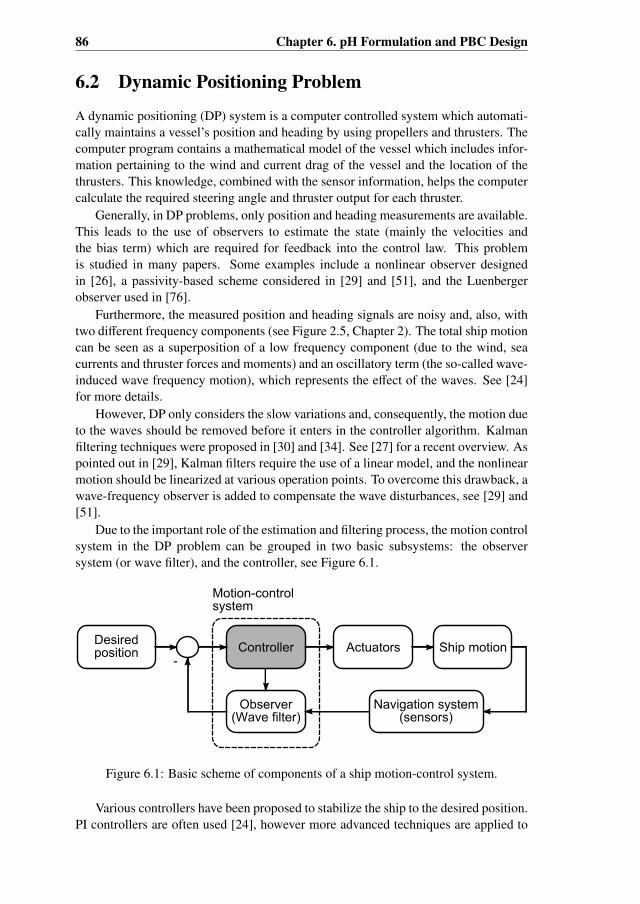
86 Chapter 6. pH Formulation and PBC Design
6.2 Dynamic Positioning Problem
A dynamic positioning (DP) system is a computer controlled system which automati-cally maintains a vessel’s position and heading by using propellers and thrusters. Thecomputer program contains a mathematical model of the vessel which includes infor-mation pertaining to the wind and current drag of the vessel and the location of thethrusters. This knowledge, combined with the sensor information, helps the computercalculate the required steering angle and thruster output for each thruster.
Generally, in DP problems, only position and heading measurements are available.This leads to the use of observers to estimate the state (mainly the velocities andthe bias term) which are required for feedback into the control law. This problemis studied in many papers. Some examples include a nonlinear observer designedin [26], a passivity-based scheme considered in [29] and [51], and the Luenbergerobserver used in [76].
Furthermore, the measured position and heading signals are noisy and, also, withtwo different frequency components (see Figure 2.5, Chapter 2). The total ship motioncan be seen as a superposition of a low frequency component (due to the wind, seacurrents and thruster forces and moments) and an oscillatory term (the so-called wave-induced wave frequency motion), which represents the effect of the waves. See [24]for more details.
However, DP only considers the slow variations and, consequently, the motion dueto the waves should be removed before it enters in the controller algorithm. Kalmanfiltering techniques were proposed in [30] and [34]. See [27] for a recent overview. Aspointed out in [29], Kalman filters require the use of a linear model, and the nonlinearmotion should be linearized at various operation points. To overcome this drawback, awave-frequency observer is added to compensate the wave disturbances, see [29] and[51].
Due to the important role of the estimation and filtering process, the motion controlsystem in the DP problem can be grouped in two basic subsystems: the observersystem (or wave filter), and the controller, see Figure 6.1.
Figure 6.1: Basic scheme of components of a ship motion-control system.
Various controllers have been proposed to stabilize the ship to the desired position.PI controllers are often used [24], however more advanced techniques are applied to

6.3. Ship Model in Port-Hamiltonian Framework 87
this problem resulting in interesting control algorithms. Backstepping design, whichalso includes the observer stage, is presented in [26] and [74]. In [51] the stabilityof a PD-type controller with a passive observer is proved using a separation principleargument. Recently, sampled-data control theory has also been applied to the DPproblem for designing the control law [42]. As mentioned at the start of this chapter,we assume that the estimation and filtering problem has been solved and our focus isthe control design for dynamic positioning using the port-Hamiltonian framework.
6.3 Ship Model in Port-Hamiltonian Framework
6.3.1 Ship Model in Cartesian CoordinatesWe recall here the vessel model from Chapter 2. In this chapter, we consider a modelin the following form.[
ην
]=
[O3 J(ψ)O3 −M−1D
] [ην
]+
[O3
M−1
]τ +
[O3
M−1JT (ψ)
]b. (6.9)
The details of the vectors and the matrices in (6.9) are given in Chapter 2. The en-vironmental disturbances due to the sea currents, waves, and wind are represented byb = [b1 b2 b3]T ∈ R3 in the Earth-fixed reference frame. This bias term is constantin the Earth-fixed reference frame, under assumption of constant or slowly varyingcurrents.
In this chapter, it is assumed that these natural effects (sometimes called bias forcesand moments), which can also be modeled as a first-order Markov process, [24, Chap-ter 3, page:89], are either known or an estimate of the bias vector is available. Weassume that the measurement system gives us noise free position and orientation mea-surements and that the wave frequency (WF) components from the measured outputare filtered or estimated. Hence, in this chapter, we skip the dynamics of the bias andthe WF components.
The main goal in the dynamic positioning problem is to stabilize the ship in a givenη-coordinate. Without loss of generality, our objective is to design an appropriate con-trol law τwhich stabilizes the system to the origin (x, y, ψ) = (0, 0, 0). Additionally, asthe measurement of the relative velocity vector is not available, the control law shouldbe independent of ν, and must be able to reject unknown disturbances or uncertainties.
6.3.2 Ship Model in Port-Hamiltonian CoordinatesWe can write the system described in (6.9) in a PHS form (6.1) by using as a statexT = [qT , pT ] ∈ R6, where q = [q1 q2 q3]T ∈ R3 represents the Earth-fixed positionand heading, and the momentum p = [p1 p2 p3]T ∈ R3, is defined as p = Mν.Substituting η = q and ν = M−1 p in (6.9), we get the following system
x = (J(q3) − R) ∂H + Gττ + Gb(q3)b (6.10)
with the following interconnection and damping matrices
J(q3) =
[O3 J(q3)
−JT (q3) O3
], R =
[O3 O3
O3 D
], (6.11)

88 Chapter 6. pH Formulation and PBC Design
the external connection matrices
Gτ =
[O3
I3
], Gb(q3) =
[O3
JT (q3)
], (6.12)
and the Hamiltonian function given by
H =12
pT M−1 p. (6.13)
Note that the Hamiltonian function contains only a kinetic energy term, associatedwith the momentum variable. A potential energy, artificially added by the controllerwill play a key role to stabilize the ship in the desired position. From (6.2), we observethat the passive output for the system (6.10) is the velocity vector which does notcorrespond to the actual output of the system, the position and the orientation. Thisis an important consideration for the control design, especially for the dynamic IDA-PBC control design in Section 6.5.
Two different energy functions are proposed in this chapter. We start by illustrat-ing the methodology using a quadratic and a trigonometric Hamiltonian function andrecover a simple classical IDA-PBC controller which guarantees asymptotic stability.The energy shaping, based on a trigonometric function, improves the heading control.These controllers do not produce the desired regulation properties in the presence ofunknown disturbances. Consequently, in order to achieve the desired performance, adynamic extension is proposed, and it results in a control law that can be interpretedas a nonlinear version of the conventional PID controller. A salient feature of the pro-posed controllers is that they do not require the relative velocity measurements and,thanks to a dynamic extension, they also ensure a good regulation behavior even inpresence of disturbances or unknown (or non-estimated) terms.
6.4 Classical IDA-PBC DesignA family of output feedback controllers can be obtained via the IDA-PBC methodol-ogy. In the design process, a nominal case is considered (i.e., where the disturbancesare assumed to be completely known), and then the stability against an unknown dis-turbance vector is also analyzed.
As presented in Section 6.1, the control laws are obtained from matching the dy-namical system (6.10) with the target dynamics (6.3). To solve this, the desired inter-connection matrix is fixed as in (6.10), i.e.,
Jd =
[O3 J(q3)
−JT (q3) O3
], (6.14)
the dissipation matrix set as
Rd =
[O3 O3
O3 Rp
], (6.15)
where Rp ∈ R3×3 is a symmetric positive definite matrix (Rp = RT
p > 0), and the closedloop energy function, Hd(x), is shaped as
Hd(q, p) = Ψ(q) +12
pT M−1 p, (6.16)
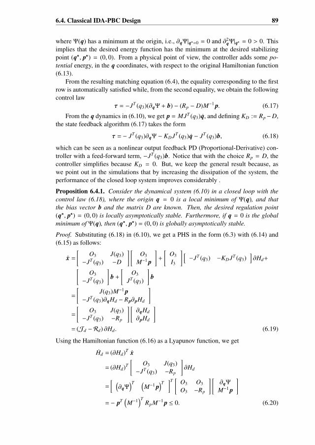
6.4. Classical IDA-PBC Design 89
where Ψ(q) has a minimum at the origin, i.e., ∂qΨ|q∗=0 = 0 and ∂2qΨ|q∗ = 0 > 0. This
implies that the desired energy function has the minimum at the desired stabilizingpoint (q∗, p∗) = (0, 0). From a physical point of view, the controller adds some po-tential energy, in the q coordinates, with respect to the original Hamiltonian function(6.13).
From the resulting matching equation (6.4), the equality corresponding to the firstrow is automatically satisfied while, from the second equality, we obtain the followingcontrol law
τ = −JT (q3)(∂qΨ + b) − (Rp − D)M−1 p. (6.17)
From the q dynamics in (6.10), we get p = MJT (q3)q, and defining KD := Rp−D,the state feedback algorithm (6.17) takes the form
τ = − JT (q3)∂qΨ − KDJT (q3)q − JT (q3)b, (6.18)
which can be seen as a nonlinear output feedback PD (Proportional-Derivative) con-troller with a feed-forward term, −JT (q3)b. Notice that with the choice Rp = D, thecontroller simplifies because KD = 0. But, we keep the general result because, aswe point out in the simulations that by increasing the dissipation of the system, theperformance of the closed loop system improves considerably .
Proposition 6.4.1. Consider the dynamical system (6.10) in a closed loop with thecontrol law (6.18), where the origin q = 0 is a local minimum of Ψ(q), and thatthe bias vector b and the matrix D are known. Then, the desired regulation point(q∗, p∗) = (0, 0) is locally asymptotically stable. Furthermore, if q = 0 is the globalminimum of Ψ(q), then (q∗, p∗) = (0, 0) is globally asymptotically stable.
Proof. Substituting (6.18) in (6.10), we get a PHS in the form (6.3) with (6.14) and(6.15) as follows:
x =
[O3 J(q3)
−JT (q3) −D
] [O3
M−1 p
]+
[O3
I3
] [−JT (q3) −KDJT (q3)
]∂Hd+[
O3
−JT (q3)
]b +
[O3
JT (q3)
]b
=
[J(q3)M−1 p
−JT (q3)∂qHd − Rp∂pHd
]=
[O3 J(q3)
−JT (q3) −Rp
] [∂qHd
∂pHd
]= (Jd − Rd) ∂Hd. (6.19)
Using the Hamiltonian function (6.16) as a Lyapunov function, we get
Hd = (∂Hd)T x
= (∂Hd)T[
O3 J(q3)−JT (q3) −Rp
]∂Hd
=
[ (∂qΨ
)T (M−1 p
)T]T
[O3 O3
O3 −Rp
] [∂qΨ
M−1 p
]= − pT
(M−1
)TRpM−1 p ≤ 0. (6.20)
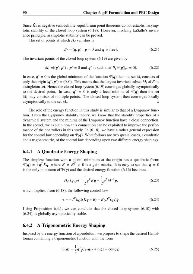
90 Chapter 6. pH Formulation and PBC Design
Since Hd is negative semidefinite, equilibrium point theorems do not establish asymp-totic stability of the closed loop system (6.19). However, invoking LaSalle’s invari-ance principle, asymptotic stability can be proved.
The set of points at which Hd vanishes is
El =(q, p) : p = 0 and q is free. (6.21)
The invariant points of the closed loop system (6.19) are given by
Ml =(q∗, p∗) : p∗ = 0 and q∗ is such that ∂qΨ(q)|q∗ = 0. (6.22)
In case, q∗ = 0 is the global minimum of the function Ψ(q) then the set Ml consists ofonly the origin (q∗, p∗) = (0, 0). This means that the largest invariant subset Ml of El isa singleton set. Hence the closed loop system (6.19) converges globally asymptoticallyto the desired point. In case, q∗ = 0 is only a local minima of Ψ(q) then the setMl may consists of multiple points. The closed loop system then converges locallyasymptotically to the set Ml.
The role of the energy function in this study is similar to that of a Lyapunov func-tion. From the Lyapunov stability theory, we know that the stability properties of adynamical system and the minima of the Lyapunov function have a close connection.In the sequel, we explain how this connection can be exploited to improve the perfor-mance of the controllers in this study. In (6.18), we have a rather general expressionfor the control law depending on Ψ(q). What follows are two special cases, a quadraticand a trigonometric, of the control law depending upon two different energy shapings.
6.4.1 A Quadratic Energy ShapingThe simplest function with a global minimum at the origin has a quadratic form:Ψ(q) = 1
2 qT Kq, where K = KT > 0 is a gain matrix. It is easy to see that q = 0is the only minimum of Ψ(q) and the desired energy function (6.16) becomes
Hd1(q, p) =12
qT Kq +12
pT M−1 p, (6.23)
which implies, from (6.18), the following control law
τ = −JT (q3)(Kq + b) − KDJT (q3)q. (6.24)
Using Proposition 6.4.1, we can conclude that the closed loop system (6.10) with(6.24), is globally asymptotically stable.
6.4.2 A Trigonometric Energy ShapingInspired by the energy function of a pendulum, we propose to shape the desired Hamil-tonian containing a trigonometric function with the form
Ψ(q) =12
qT12C12q12 + c3(1 − cos q3), (6.25)
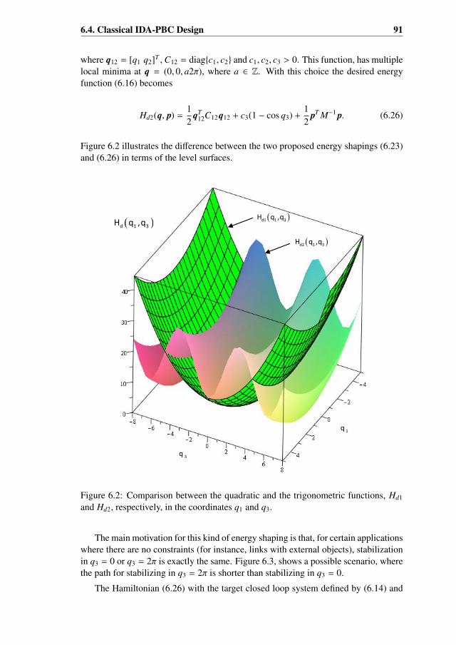
6.4. Classical IDA-PBC Design 91
where q12 = [q1 q2]T , C12 = diagc1, c2 and c1, c2, c3 > 0. This function, has multiplelocal minima at q = (0, 0, a2π), where a ∈ Z. With this choice the desired energyfunction (6.16) becomes
Hd2(q, p) =12
qT12C12q12 + c3(1 − cos q3) +
12
pT M−1 p. (6.26)
Figure 6.2 illustrates the difference between the two proposed energy shapings (6.23)and (6.26) in terms of the level surfaces.
d 1 3H q ,q
3q
1q
d1 1 3H q ,q
d2 1 3H q ,q
22
11
Figure 6.2: Comparison between the quadratic and the trigonometric functions, Hd1
and Hd2, respectively, in the coordinates q1 and q3.
The main motivation for this kind of energy shaping is that, for certain applicationswhere there are no constraints (for instance, links with external objects), stabilizationin q3 = 0 or q3 = 2π is exactly the same. Figure 6.3, shows a possible scenario, wherethe path for stabilizing in q3 = 2π is shorter than stabilizing in q3 = 0.
The Hamiltonian (6.26) with the target closed loop system defined by (6.14) and
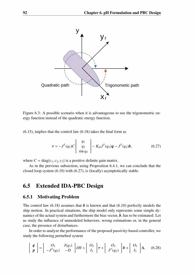
92 Chapter 6. pH Formulation and PBC Design
Trigonometic pathQuadratic path
yyr
xr
Figure 6.3: A possible scenario when it is advantageous to use the trigonometric en-ergy function instead of the quadratic energy function.
(6.15), implies that the control law (6.18) takes the final form as
τ = −JT (q3)C
q1
q2
sin q3
− KDJT (q3)q − JT (q3)b, (6.27)
where C = diagc1, c2, c3 is a positive definite gain matrix.As in the previous subsection, using Proposition 6.4.1, we can conclude that the
closed loop system (6.10) with (6.27), is (locally) asymptotically stable.
6.5 Extended IDA-PBC Design
6.5.1 Motivating Problem
The control law (6.18) assumes that b is known and that (6.10) perfectly models theship motion. In practical situations, the ship model only represents some simple dy-namics of the actual system and furthermore the bias vector, b, has to be estimated. Letus study the influence of unmodeled behaviors, wrong estimations or, in the generalcase, the presence of disturbances.
In order to analyze the performance of the proposed passivity-based controller, westudy the following perturbed system[
qp
]=
[O3 J(q3)
−JT (q3) −D
]∂H +
[O3
I3
]τ +
[O3
JT (q3)
]b +
[O3
I3
]∆, (6.28)
6.5. Extended IDA-PBC Design 93
where ∆ ∈ R3 is a vector which represents the disturbances. As a first approximation,and only to motivate the use of the extended dynamics, we consider this vector as aconstant.
The system (6.28) in a closed loop with (6.18) results in the following system[qp
]=
[O3 J(q3)
−JT (q3) −Rp
]∂Hd +
[O3
I3
]∆, (6.29)
which has an equilibrium point which satisfies ∂Ψ|q=q∗ = J(q∗3)∆ and p∗ = 0. Itimplies that in presence of disturbances, the closed-loop system (6.28) with controllaw (6.18) has a different equilibrium than (0, 0). However, stability should also befurther analyzed.
Moreover, in the special case where the disturbances are also affected by JT (q3)given by[
qp
]=
[O3 J(q3)
−JT (q3) −D
]∂H +
[O3
I3
]τ +
[O3
JT (q3)
]b +
[O3
JT (q3)
]∆, (6.30)
it can be seen that some stability properties still remain. With the control law (6.24),global asymptotic stability can be proved by shifting the Hamiltonian function to thenew equilibrium point, i.e., with
Hd1 =12
(q − q∗)T K(q − q∗) +12
pT M−1 p (6.31)
as a Lyapunov function, where q∗ = K−1∆. See Appendix A for more details.Similarly, the control law (6.27) derived by using the trigonometric energy shaping
in (6.30), gives the following closed-loop system[qp
]=
[O3 J(q3)
−JT (q3) −Rp
] [∂qHd2
∂pHd2
]+
[O3
JT (q3)
]∆, (6.32)
where ∂qHd2 = C
q1
q2
sin q3
and ∂pHd2 = M−1 p. The new set of equilibrium points of
(6.32) is
q∗ =
[∆1
c1,∆2
c2, arcsin
(∆3
c3
)− 2kπ
]T
, and p∗ = 0, k ∈ Z. (6.33)
The new set of equilibrium points (6.33) is not a set of minima of (6.26). Unlike thequadratic case, shifting of (6.26) to the new equilibrium (6.33) does not make them aset of minima of the shifted Hamiltonian function. This is because of the presence oftranscendental term in (6.26). Therefore, we require another Hamiltonian function forthe stability analysis of (6.32).
We seek another Hamiltonian function (energy shaping) Hd2(q, p) which has aminimum value at (q∗, 0), i.e., we require
∂qHd2(q, p)|q∗ = 0, ∂pHd2(q, p)|p∗ = 0, and ∂2Hd2(q, p)|(q∗,p∗) > 0. (6.34)
94 Chapter 6. pH Formulation and PBC Design
Let us define
Hd2 (q, p) =12
c1
(q1 −
∆1
c1
)2
+12
c2
(q2 −
∆2
c2
)2
+ c3ψ3(q3) +12
pT M−1 p, (6.35)
where ψ3(q3) is such that
∂q3 ψ3|q∗3 = 0,
⇒ ∂q3 ψ3 = sin q3 −∆3
c3.
Integrating both sides,
ψ3(q3) = − cos q3 −∆3
c3q3 + e1,
where e1 is a constant of integration. Without loss of generality, we take e1 = 1, then
ψ3(q3) = 1 − cos q3 −∆3
c3q3. (6.36)
Therefore, the new desired energy function is
Hd2(q, p) =12
c1
(q1 −
∆1
c1
)2
+12
c2
(q2 −
∆2
c2
)2
+ c3
(1 − cos q3 −
∆3
c3q3
)+
12
pT M−1 p.
(6.37)
The Hessian of Hd2(q, p) is given by
∂2Hd2 =
[∂2
qHd2 ∂2qpHd2
∂2pqHd2 ∂2
pHd2
]=
[∂2
qHd2 O3
O3 M−1
],
where
∂2qHd2 =
c1 0 00 c2 00 0 c3 cos q3
.Using the Schur complement argument, the Hessian, ∂2Hd2|(q∗,p∗) is positive definiteiff ∂2
qHd2|(q∗,p∗) > 0. This requires
c3 cos q∗3 > 0,
⇒ c3 cos(sin−1 ∆3
c3
)> 0,
⇒
√1 −
(∆3
c3
)2
> 0,
⇒∆3
c3< 1.
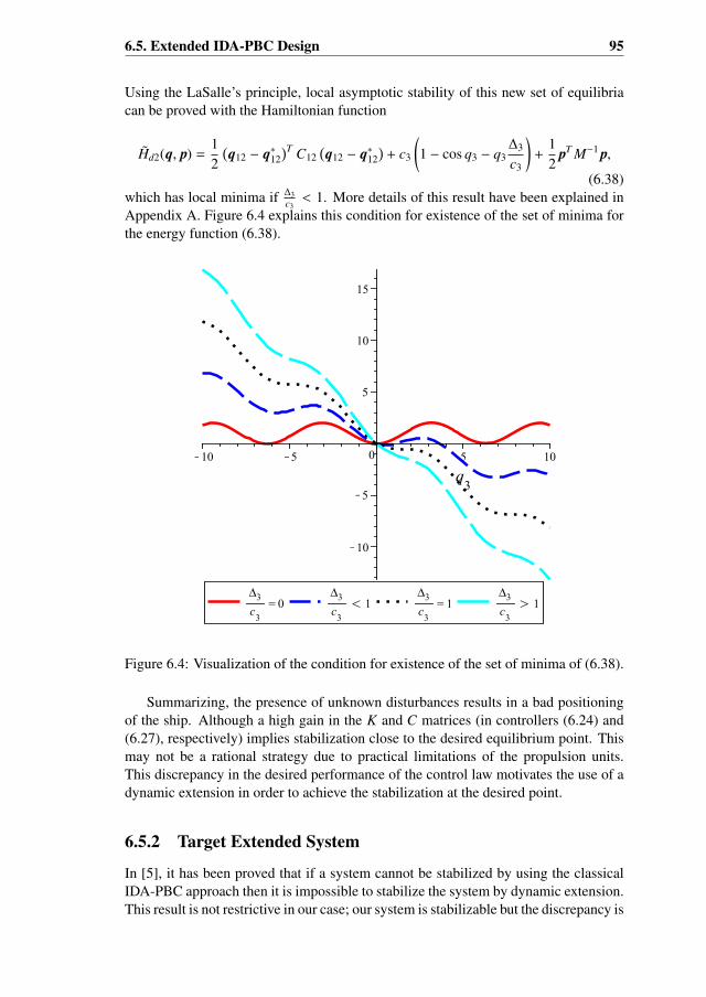
6.5. Extended IDA-PBC Design 95
Using the LaSalle’s principle, local asymptotic stability of this new set of equilibriacan be proved with the Hamiltonian function
Hd2(q, p) =12
(q12 − q∗12
)T C12(q12 − q∗12
)+ c3
(1 − cos q3 − q3
∆3
c3
)+
12
pT M−1 p,
(6.38)which has local minima if ∆3
c3< 1. More details of this result have been explained in
Appendix A. Figure 6.4 explains this condition for existence of the set of minima forthe energy function (6.38).
Figure 6.4: Visualization of the condition for existence of the set of minima of (6.38).
Summarizing, the presence of unknown disturbances results in a bad positioningof the ship. Although a high gain in the K and C matrices (in controllers (6.24) and(6.27), respectively) implies stabilization close to the desired equilibrium point. Thismay not be a rational strategy due to practical limitations of the propulsion units.This discrepancy in the desired performance of the control law motivates the use of adynamic extension in order to achieve the stabilization at the desired point.
6.5.2 Target Extended System
In [5], it has been proved that if a system cannot be stabilized by using the classicalIDA-PBC approach then it is impossible to stabilize the system by dynamic extension.This result is not restrictive in our case; our system is stabilizable but the discrepancy is
96 Chapter 6. pH Formulation and PBC Design
that it does not stabilize to the desired equilibrium point. To overcome this drawback,we introduce an integral action by dynamic extension.
A dynamic extension for a non passive output, maintaining the port-Hamiltonianstructure, is possible by means of a change of coordinates. The controller is designedfor a nominal case, without disturbances, and then the presence of unknown termsis analyzed. Following the idea in [20], we introduce a new state variable, ze ∈ R
3,which is used to enforce the equilibrium point of the closed-loop system to the desiredone, and a change of variables z = f (q, p, ze). We define the target system, with theform of (6.6), as q
zze
=
O3 J(q3) J(q3)−JT (q3) −Rz O3
−JT (q3) O3 O3
∂qHde
∂zHde
∂ze Hde
, (6.39)
where Rz = RTz ≥ 0, is a 3 × 3 matrix to be defined. The desired Hamiltonian function
is defined as
Hde(q, z, ze) = Ψ(q) +12
zT M−1 z +12
zTe Ke ze (6.40)
where Ke = diagke1, ke2, ke3 > 0. As earlier in the classical IDA-PBC design, Ψ(q)must be designed with a minimum in the desired regulation point. Then, the Hamilto-nian function (6.40) has a minimum at (q∗, z∗, z∗e) = (q∗, 0, 0).
Matching the q dynamics, from (6.10) and (6.39), the change of variables z isdefined as
z = p− MKe ze. (6.41)
The state feedback control law is obtained from the second row of (6.39) and the timederivative of (6.41),
τ = −KPJT (q3)∂qΨ − KDM−1 p + KI ze − JT (q3)b (6.42)
ze = −JT (q3)∂qΨ (6.43)
where we define
KP := (MKe + I3), (6.44)
KD := Rz − D, (6.45)
KI := Ke. (6.46)
Similarly to the classical IDA-PBC controller in the previous section, using p =
MJT (q3)q, the control law (6.42)-(6.43) takes the following form
τ = −KPJT (q3)∂qΨ − KI
∫JT (q3)∂qΨdt − KDJT (q3)q − JT (q3)b (6.47)
which has the same structure as a nonlinear PID controller with a feed-forward term,−JT (q3)b.
Proposition 6.5.1. Assume that q is measurable, and that the disturbances vector band the matrices M and D are known. If Ke = diagke1, ke2, ke3 > 0, and Ψ(q) has
6.5. Extended IDA-PBC Design 97
a (local) minimum at the origin, q = 0, then the system (6.10) in a closed loop with(6.47), is (locally) asymptotically stable at the point (q, z, ze) = (0, 0, 0).
Furthermore, if q = 0 is a global minimum of Ψ(q), then the origin of (6.47) isglobally asymptotically stable.
Proof. The closed-loop system (6.10) with (6.47) takes the form of (6.39). Then, theHamiltonian function (6.40) is a Lyapunov-candidate function and its time derivativeis
Hde = −zT(M−1
)TRzM−1 z ≤ 0. (6.48)
Then, the stability can be proved invoking LaSalle’s invariance principle as we alreadyshow in proof of Proposition 6.4.1.
Equation (6.47) is a rather general formulation of the control law. What followsare two special cases depending on two different formulations of the energy shaping(6.40).
6.5.3 A Quadratic Energy Shaping
Let us first take the same quadratic energy shaping as in Section 6.4, Ψ(q) = 12 qT Kq
with K = diagk1, k2, k3 > 0, the Hamiltonian function (6.40) becomes
Hde1(q, z, ze) =12
qT Kq +12
zT M−1 z +12
zTe Ke ze. (6.49)
with a global minimum at the origin, (0, 0, 0). The control law (6.42)-(6.43) becomes
τ = −KPJT (q3)Kq + KI ze − KDJT (q3)q − JT (q3)b (6.50)
ze = −JT (q3)Kq. (6.51)
From Proposition 6.5.1 the controller (6.50)-(6.51) ensures the global asymptotic sta-bility.
6.5.4 A Trigonometric Energy Shaping
The trigonometric energy shaping proposed in the previous section can also be con-sidered for the extended controller. Taking again
Ψ(q) =12
qT12C12q12 + c3 (1 − cos q3) , (6.52)
where q12 = [q1 q2]T and C12 = diagc1, c2, and c1, c2, c3 > 0 the desired Hamiltonianfunction (6.40) becomes
Hde2(q, z, ze) =12
qT12C12q12 + c3 (1 − cos q3) +
12
zT M−1 z +12
zTe Ke ze. (6.53)
As previously mentioned, this function has multiple local minima at q∗ = (0, 0, a2π),a ∈ Z. Using Proposition 6.5.1, this case ensures local asymptotic stability, and the
98 Chapter 6. pH Formulation and PBC Design
control law (6.42)-(6.43) becomes
τ = −KPJT (q3)C
q1
q2
sin q3
+ KI ze − KDJT (q3)q − JT (q3)b (6.54)
ze = −JT (q3)C
q1
q2
sin q3
(6.55)
where C = diagc1, c2, c3.
6.5.5 Analysis in Presence of DisturbancesThe main contribution of the extended dynamics excels in the presence of unknowndisturbances. As before, let us analyze the closed-loop system in the presence ofdisturbances. First, we consider constant (or, at least, very slow) disturbances. Takingthe perturbed system (6.28) with the designed control law (6.47), we obtain q
zze
=
O3 J(q3) J(q3)−JT (q3) −Rz O3
−JT (q3) O3 O3
∂qΨ
M−1 zKe ze
+
O3
I3
O3
∆. (6.56)
From the ze dynamics, and due to ∂qΨ|q∗ = 0, this system has the following equilib-rium point3
q∗ = 0 (6.57)
z∗ = MR−1z ∆ (6.58)
z∗e = −KeR−1z ∆. (6.59)
Notice that, contrary to the classical controller as discussed in Section 6.5.1, in thepresence of unknown disturbances, the origin is still the equilibrium in the positioncoordinates.
The question that now arises is about the stability of (6.56). A simple stabilityanalysis is possible using the error coordinates z = z − z∗ and ze = ze − z∗e. Shiftingthe energy function (6.40) to the new equilibria, we get
Hde(q, z, ze) = Ψ(q) +12
zT M−1 z +12
zTe Ke ze, (6.60)
and (6.56) can be written asq˙z˙ze
=
O3 J(q3) J(q3)−JT (q3) −Rz O3
−JT (q3) O3 O3
∂qΨ
M−1 zKe ze
. (6.61)
This closed-loop system still has the desired structure (6.6), with a energy functionwhich has a minimum at (6.57)-(6.59). The asymptotic stability is automatically guar-anteed.
3Notice that for the case of the trigonometric controller, the equilibria become q∗ = (0, 0, a2π).
6.6. Simulations 99
In a more realistic case, the disturbance could be considered as a vector whichdepends on time, i.e., ∆ = ∆(t). Then, we can no longer study the stability of anequilibrium point, and we only can expect that the solution of the system becomesbounded due to the special structure of the closed-loop system, that can be seen as aforced oscillator with damping in the z coordinates.
6.6 SimulationsIn order to test the performance of the designed controllers we performed some nu-merical simulations. For this validation we used the data of a supply ship from [26].The (Bis-scaled non-dimensional [24]) matrices M and D are given by
M =
1.1274 0 00 1.8902 −0.07440 −0.0744 0.1278
and
D =
0.0358 0 00 0.1183 −0.01240 −0.0124 0.0308
.The bias vector has been set to b = [0.05, 0.05, 0.01]T . For all simulations, we consid-ered that the initial conditions of the ship are (q1, q2) = (−10,−10), and the headingangle q3 = 4 rad, and the desired stabilization position is the origin. The desired head-ing direction is along the positive x-axis. More generally, the starting heading angleis set greater than π to show the ability of the so-called trigonometric controller tostabilize to the closer minimum, in this case 2π.
6.6.1 Simulation Results for the classical IDA-PBC designIn this subsection, we present the simulation results for the classical (quadratic andtrigonometric) control laws (6.24) and (6.27), respectively. The gain matrices we usedare K = C = diag0.05, 0.05, 0.01 and Rp = diag0.75, 0.75, 0.1. Precisely, for thissystem, we enlarged the damping (about one order of magnitude in the first and thirdcomponents), to improve the performance. In Figure 6.5 we show the trajectoriesof the same classical controller (the quadratic case) with extra dissipation, settingRp to the values proposed before, and keeping the original damping, Rp = D. Thiscomparison justifies the use of the extra damping to obtain more suitable paths.
Figure 6.6 shows the trajectories of the position coordinates q1 and q2, and theheading angle, q3, of the quadratic and the trigonometric versions. Both controllersstabilize the ship at the desired position and angle. The notable point is the differencein the orientation profiles. While the quadratic controller stabilizes the heading angleat q3 = 0, the trigonometric controller does so at q3 = 2π.
Figure 6.7 compares the trajectories in the q1q2-plane for two versions of the clas-sical IDA-PBC design. In both cases, the performance is similar but, even though thecontrollers for the q1 and q2 coordinates are the same (with the same gain values),
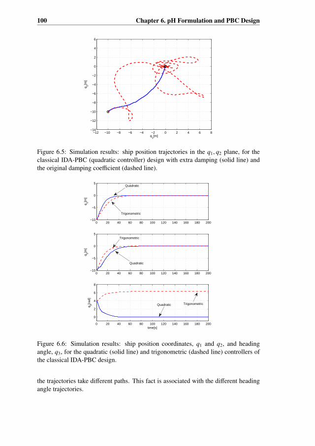
100 Chapter 6. pH Formulation and PBC Design
−12 −10 −8 −6 −4 −2 0 2 4 6 8−14
−12
−10
−8
−6
−4
−2
0
2
4
6
q1[m]
q 2[m]
Figure 6.5: Simulation results: ship position trajectories in the q1, q2 plane, for theclassical IDA-PBC (quadratic controller) design with extra damping (solid line) andthe original damping coefficient (dashed line).
0 20 40 60 80 100 120 140 160 180 200−10
−5
0
5
q 1[m]
0 20 40 60 80 100 120 140 160 180 200−10
−5
0
5
q 2[m]
0 20 40 60 80 100 120 140 160 180 200
0
2
4
6
8
q 3[rad
]
time[s]
Quadratic
Trigonometric
Quadratic
Trigonometric
TrigonometricQuadratic
Figure 6.6: Simulation results: ship position coordinates, q1 and q2, and headingangle, q3, for the quadratic (solid line) and trigonometric (dashed line) controllers ofthe classical IDA-PBC design.
the trajectories take different paths. This fact is associated with the different headingangle trajectories.
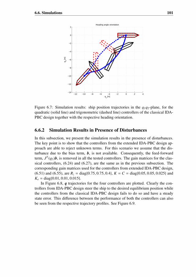
6.6. Simulations 101
−12 −10 −8 −6 −4 −2 0 2 4−14
−12
−10
−8
−6
−4
−2
0
2
q1 [m]
q 2 [m]
Heading angle orientation
Figure 6.7: Simulation results: ship position trajectories in the q1q2-plane, for thequadratic (solid line) and trigonometric (dashed line) controllers of the classical IDA-PBC design together with the respective heading orientation.
6.6.2 Simulation Results in Presence of DisturbancesIn this subsection, we present the simulation results in the presence of disturbances.The key point is to show that the controllers from the extended IDA-PBC design ap-proach are able to reject unknown terms. For this scenario we assume that the dis-turbance due to the bias term, b, is not available. Consequently, the feed-forwardterm, JT (q3)b, is removed in all the tested controllers. The gain matrices for the clas-sical controllers, (6.24) and (6.27), are the same as in the previous subsection. Thecorresponding gain matrices used for the controllers from extended IDA-PBC design,(6.51) and (6.55), are Rz = diag0.75, 0.75, 0.4, K = C = diag0.05, 0.05, 0.025 andKe = diag0.01, 0.01, 0.015.
In Figure 6.8, q trajectories for the four controllers are plotted. Clearly the con-trollers from IDA-PBC design steer the ship to the desired equilibrium position whilethe controllers from the classical IDA-PBC design fails to do so and have a steadystate error. This difference between the performance of both the controllers can alsobe seen from the respective trajectory profiles. See Figure 6.9.

102 Chapter 6. pH Formulation and PBC Design
0 20 40 60 80 100 120 140 160 180 200−10
−5
0
q1[m]
0 20 40 60 80 100 120 140 160 180 200−10
−5
0
q2[m]
0 20 40 60 80 100 120 140 160 180 200
0
2
4
6
8
q3[rad]
time[s]
Extended controllers
Classical controllers
Extended controllers
Classical controllers
Extended Trig.
Classical Quad.
Classical Trig.
Extended Quad.
Figure 6.8: Simulation results: ship position coordinates, q1 and q2, and headingangle, q3, for the both the quadratic and trigonometric versions of the controllers fromthe classical and extended IDA-PBC designs.
−12 −10 −8 −6 −4 −2 0 2 4−12
−10
−8
−6
−4
−2
0
2
4
q1[m]
q 2[m]
Extended Quad.
ClassicalQuad.
Extended Trig.
Classical Trig.
Figure 6.9: Simulation results: ship position trajectories in the q1, q2 plane, for theboth the quadratic and trigonometric versions of the controllers from the classical andextended IDA-PBC designs.
6.7 Conclusions
A passivity-based approach called IDA-PBC is used to obtain a set of output feedbackcontrollers for the dynamic positioning of a ship. This methodology is based on the
6.7. Conclusions 103
port-Hamiltonian description which gives a physical interpretation of the dynamicalsystems. Under this point of view, the controller design problem is addressed as toshape the energy function of the closed loop system. After a general formulation wepropose two different controllers: first with a quadratic energy function and second,inspired by the physics of a pendulum, with a trigonometric energy function. Also, thepresence of disturbances is studied and it turns out that the control laws obtained byusing the classical IDA-PBC methodology, do not stabilize the system at the desiredposition. This discrepancy is the starting point for a second set of controllers whichconsist of a dynamic extension of the system which provides stability at the desiredregulation point, also in presence of disturbances. Simulations are done to validateand compare the performance of the controllers designed.
It is worth mentioning that the obtained control laws, with a general form of statefeedback, can be easily converted to output feedback algorithms that only requirethe position measurement. Furthermore, they exhibit a simple structure that can beinterpreted as non-linear versions of PID controllers. An important observation is thatthe trigonometric energy shaping improves the heading angle control. We also observethat by keeping the differential term, which physically increases the damping effect,in the controller formulation helps in getting a smoother trajectory profile.
Future work can be aimed at determining other energy functions, Ψ(q), to improvethe performance, as well as to consider the optimization of the resulting path. Furtheranalysis depending on the nature of the disturbance vector (including the wave fre-quency and wind models) is required. Also, this work could be a starting point for anew design, using the port-Hamiltonian perspective, of the complete motion-controlsystem (controller and observer) for a DP problem.

104
Chapter 7Conclusions andRecommendations for FutureWork
In this chapter, we summarize the main conclusions of this work and present somerecommendations for future work based on our knowledge and experiences acquiredduring the process of reaching to this point. The first major topic studied in this thesisis the stability analysis of a special type of nonlinear system in which nonlinearityappears only in the dynamics of a single state variable. The study is based on theSDC framework which transforms the nonlinear system in a pseudo-linear form witha state dependent system matrix. The stability analysis of such systems is based onthe properties of the system matrix. From the perspective of the DP system we areinterested in the asymptotic behavior of the system. The local asymptotic stability ofthe system is easy to establish, the major concern always remains the analysis of theglobal asymptotic stability.
From the first counterexample discussed in Section 3.4.1, we can conclude that theconditions that the system matrix is continuous, pointwise Hurwitz, and exponentiallybounded are not sufficient to ascertain the global asymptotic stability of the pseudo-linear system. In the prototype vessel model, the system matrix is a periodic functionof the heading angle of the vessel. The periodicity assumption also ensures that thestates of the system are bounded, i.e., they will not blow up at finite time. Furtherresearch has proved that the extended set of conditions that the system matrix is con-tinuous, pointwise Hurwitz, exponentially bounded, and periodic does not constitutethe set of sufficient conditions for the global asymptotic stability of the pseudo-linearsystem. This fact is explained in the second counterexample presented in Section3.5.1. This study concludes that more research is required to explore the set of suf-ficient conditions which establish the global asymptotic stability of the pseudo-linearsystems with a system matrix depending on a single state variable.
The periodicity property of the vessel model has lured us to combine the Lyapunov
105
106 Chapter 7. Conclusions and Recommendations for Future Work
stability theory with the LMIs to come up with a new approach to prove the globalasymptotic stability of the pseudo-linear system which has a periodic system matrix.This approach has proved successful to establish the global asymptotic stability of thevessel model, in particular. Further research is required to investigate the additionalfeatures like for instance, the best solutions of the LMI feasibility problem, the impactof the number of LMIs on the solutions of the LMI feasibility problem, conditions forexistence and non-existence of the solutions of the LMI feasibility problem, etc.
We present the SDARE technique for control design of the vessel model. Thedesign objective is to stabilize the vessel at the desired equilibrium point. The SDAREtechnique gives a state feedback controller which means that the complete state ofthe system should be known. This is not the case for the vessel model in this workas only the noisy position and heading measurements are available through sensors(GPS and gyro). So it is required to estimate the remaining states of the vessel model.We have also used the SDARE technique to address the estimation problem. TheSDARE technique has many characteristic features. It addresses the performance ofthe controller and the observer by specifying a performance index. The state andthe control weights can be adjusted to influence the performance. For instance, anincrease in the state weighting matrix Q results in a faster regulation of the vesselat the expense of a greater control effort. Generally, the SDC parametrization is notunique and this feature offers an extra degree of freedom for design and performanceimprovements. While the technique offers ways to use the results from linear systemtheory, it maintains the nonlinear character of the system which is not the case inlinearization methods like the extended Kalman filter (EKF) etc.
The simulation results show promising performance of the SDARE techniquewhen applied to address the regulation problem of a DP vessel. The controller andthe observer gains can be tuned by using the weighting matrices, to obtain the desiredperformance. This study is limited to the regulation problem of the DP vessel. An ex-tension of the SDARE technique to address the path following and trajectory trackingproblems of the DP vessel remains still an open research topic.
We present the FSI method which is a fast solution method for the specific typeof the SDARE associated with a pseudo-linear system whose system matrix dependson a single state variable in a periodic way. This method is based on the Fourierseries and involves the concept of interpolation. The emphasis of the FSI method ison offline computation of the Fourier series coefficients. It has been shown that itmakes the online computation of the solution of the SDARE faster by reducing theonline computations. The method is particularly useful for the systems having a smalltime constant or fast dynamic response. For such systems, the actuators are requiredto have a faster dynamic response than the system they are controlling. The methodwas motivated by the periodicity of the pseudo-linear vessel model. The vessel systemin this work is a slow system (with a large time constant), the FSI method has showngood results in comparison with the MATLAB routine “care” which uses the Schurdecomposition to solve the SDARE. This work is limited to just one application of theFSI method on the vessel model. The search for more applications of the FSI methodon physical systems is still open for future research.
In this work, the use of the port-Hamiltonian system formulation to study the con-trol design problem of the DP vessel has revealed some important and interesting
107
features. The Hamiltonian (storage) function is a powerful component in this formu-lation. We have seen that it not only simplifies the stability analysis but also offersmore options to improve the performance of the controller. This can be done by usingdifferent formulations of the Hamiltonian function to design different controllers. Theperformance of the controllers can then be analyzed to see which one suits the desiredperformance objective. This fact is clear from the trigonometric and quadratic formu-lations of the Hamiltonian function. A better heading control of the vessel is obtainedfrom the trigonometric controller than the quadratic controller.
The dissipation (damping) matrix in the desired dynamics in the IDA-PBC designtechnique is very important from the perspective of the tuning of the controller gainmatrices. It makes it possible to manipulate the damping of the system. Through thecontroller action, we can increase the damping of the system and it eventually helpsus to steer the vessel along a stable and smooth trajectory.
This study addresses only the regulation problem with passivity based approachusing the port-Hamiltonian formulation. With the encouraging results obtained, thepossible extension of this concept to address more involved problems like path fol-lowing, trajectory tracking, and state estimation is a challenging and interesting topicfor future research.

108
Appendix AProof of Asymptotic Stability of(6.32) at (6.33)
The objective is to show that (6.33) is an asymptotically stable equilibrium point ofthe perturbed closed loop system (6.32). For convenience of the reader, we recall bothequations mentioned above.[
qp
]=
[O3 J(q3)
−JT (q3) −Rp
] [∂qHd2
∂pHd2
]+
[O3
JT (q3)
]∆, (A.1)
where
Hd2(q, p) =12
qT12C12q12 + c3(1 − cos q3) +
12
pT M−1 p. (A.2)
The equilibrium point of (A.1) is given by
q∗ =[
∆1c1
∆2c2
arcsin(
∆3c3
)− 2kπ
]T, and p∗ = 0, k ∈ Z. (A.3)
To prove the above mentioned asymptotic stability, we proceed as follows. Let usconsider the following closed loop system.[ ˙q
˙p
]=
[O3 J(q3)
−JT (q3) −Rp
] [∂qHd2
∂ pHd2
], (A.4)
where q =
q1 − q∗1q2 − q∗2
q3
, p = p, and
Hd2(q, p) =12
qT12C12 q12 + c3
(1 − cos q3 −
∆3
c3q3
)+
12
pT M−1 p. (A.5)
As a first step, we use the LaSalle’s invariance principle to prove asymptotic sta-bility of (A.4). The energy function (A.5) is a scalar valued function and its first partial
109

110 Appendix A
derivatives exist. Differentiating it w.r.t ‘t’, we get
˙Hd2 =(∂Hd2
)T ˙x
=(∂Hd2
)T[
O3 J(q3)−JT (q3) −Rp
]∂Hd2
= − pT(M−1
)TRpM−1 p ≤ 0, (A.6)
where x =
[qp
]. The set of points where ˙Hd2 = 0 is given by
El =x ∈ R6 : ˙Hd2 = 0
= p = 0 and q is free. (A.7)
The equilibrium (invariant) points of (A.4) are
q∗ =[q1, q2, q3
]T=
[0, 0, arcsin(
∆3
c3) − 2kπ
]T
, and p∗ = 0, k ∈ Z. (A.8)
The largest invariant subset Ml of El consists of the equilibrium points (A.8). Hence,LaSalle’s invariance principle implies that the closed loop system (A.4) convergeslocally asymptotically to either one of the equilibrium points.
As second step, we show that both the closed loop systems (A.1) and (A.4) areequivalent. It is a straightforward observation that q and q have the same dynamics.We show the equivalence of the dynamics of p and p.
˙p = − JT (q3)∂qHd2 − Rp∂ pHd2
= − JT (q3)∂qHd2 − Rp∂pHd2 + JT (q3)∆
= p. (A.9)
Hence, (A.1) and (A.4) are equivalent. This implies that if (A.8) is an asymptoticallystable equilibrium point of (A.4) then (A.3) is an asymptotically stable equilibriumpoint of (A.1).
Similarly, asymptotic stability of[qp
]=
[O3 J(q3)
−JT (q3) −Rp
] [∂qHd1
∂pHd1
]+
[O3
JT (q3)
]∆, (A.10)
where
Hd1(q, p) =12
qT Cq +12
pT M−1 p. (A.11)
w.r.t. the equilibrium point (q∗, p∗) = (−K−1∆, 0) follows. The asymptotic stability inthis case will be global because the point (q∗, p∗) = (−K−1∆, 0) is global minimum ofthe shifted Hamiltonian function associated with (A.11).
Appendix BGlossary
This appendix contains definitions and additional details of some notions used in thisthesis.
BIS-Scaling
Scaling is done to normalize the vessel steering equations of motion. This helps tostudy the scaled models of the vessel and then compare and analyze the performanceof the full scale vessel models. This idea is more economical both in terms of timeand money, than doing the full scale experiments in the sea. There are two main meth-ods of scaling: the Prime-system of SNAME introduced in 1950 and the Bis-systemintroduced in 1970 by Norrbin. The Prime-system uses the instantaneous velocity tonormalize the time unit. Therefore, it is not used for the DP vessels or other low speedapplications.
The Bis-system uses the length unit Lpp (length between fore and aft perpendic-
ulars), body mass density ratio µ = mρ∇
, and the time unit√
Lpp
g as the basic scalingparameters. The parameters µ, ρ, ∇, and g represent the level of buouncy, mass densityof the fluid, hull contour displacement, and acceleration due to gravity, respectively.The scaling parameters for other variables like velocity, acceleration, etc. can be foundin terms of these basic scaling parameters.
First order wave-induced forces
First order wave-induced wave forces (loads or disturbances) are forces whose mag-nitude is proportional to the wave height and their frequency is the same as that of theincident waves. These forces are also called WF forces (disturbances or loads).
Gaussian white noise process
In Chapter 2, we have mentioned that the process and measurement uncertainties arestationary Gaussian random white noise process. For the convenience of the reader,
111

112 Appendix B
some details of this concept are presented here. The vector w(t) =
w1(t)w2(t)w3(t)
consists
of three uncorrelated independent Gaussian white noise processes: w1(t), w2(t), andw3(t). This implies the mean
E(w(t)) = 0, (B.1)
and covariance
E(w(t)wT (s)
)= Wδ(t − s). (B.2)
The δ in (B.2) represents the Dirac delta (or continuous time impulse response) func-tion and is given by
δ(t − s) =
∞ if t = s0 if t , s
(B.3)
Kronecker Product
Let A ∈ Rm×n and B ∈ Rp×q. Then the Kronecker (direct or tensor) product of A and Bis defined as the matrix
A ⊗ B =
a11B · · · a1mB...
. . ....
am1B · · · amnB
∈ Rmp×nq. (B.4)
LaSalle’s Invariance Theorem (Principle)
An important result in stability theory which was independently formulated by N. N.Krasovskii and E. A. Barbashin in Russian in 1959, see [11] for its translated versionin English, and by J. P. LaSalle in 1960, see [48]. It is stated as follows
“Let Ω0 ⊂ Ω be a compact set that is positively invariant with respect to (3.2). LetV : Ω −→ R be a continuously differentiable function such that V(x) ≤ 0 in Ω0. LetE be the set of all points in Ω0 where V(x) = 0. Let M be the largest invariant set inE. Then every solution starting in Ω0 approaches M as t → ∞.”
Second order wave-induced forces
Second order wave-induced wave forces (loads or disturbances) are forces whose mag-nitude is proportional to the square of the wave height. These forces are also calledLF forces (disturbances or loads).

Bibliography
[1] M. F. Aarset, J. P. Strand, and T. I. Fossen. Nonlinear vectorial observer back-stepping with integral action and wave filtering for ships. Proceedings of IFACConference on Control Applications in Marine Systems CAMS’98, October 20-27, 1998, Fukuoka, Japan.
[2] T. Acarman. Nonlinear optimal integrated vehicle control using individual brak-ing torque and steering angle with on-line control allocation by using state-dependent Riccati equation technique. Vehicle Sysytem Dynamics, 47(2):155–177, 2009.
[3] B. D. O. Anderson. Second-order convergent algorithms for the steady-stateRiccati equation. International Journal of Control, 28(2):295–306, 1978.
[4] A. Astolfi, D. Chhabra, and R. Ortega. Asymptotic stabilization of some equi-libria of an underactuated underwater vehicle. Systems & Control Letters,45(3):193–206, 2002.
[5] A. Astolfi and R. Ortega. Dynamic extension is unnecessary for stabilizationvia interconnection and damping assignment passivity-based control. Systems &
Control Letters, 58(2):133–135, 2009.
[6] J. G. Balchen, N. A. Jenssen, and S. Sælid. Dynamic positioning using kalmanfiltering and optimal control theory. pages 183–186. Proceedings of IFAC/IFIPSymposium on Automation in Offshore Oil Field Operation,ly 6-11, 2008, Am-sterdam, The Netherlands.
[7] H. T. Banks, B. M. Lewis, and H. T. Tran. Nonlinear feedback controllers andcompensators: a state-dependent Riccati equation approach. Computational Op-timization and Applications, 37(2):177–218, 2007.
[8] S. P. Banks and K. J. Mhana. Optimal control and stabilization of nonlinearsystems. IMA Journal of Mathematical Control and Information, 9(3):179–196,1992.
113

114 BIBLIOGRAPHY
[9] P. Benner and R. Byers. An exact line search method for solving generalizedcontineous-time algebraic Riccati equation. IEEE Transactions on AutomatcControl, 43(1):101–107, 1998.
[10] W. E. Boyce and R. C. DiPrima. Elementary Differential Equations and Bound-ary Value Problems. John Wiley & Sons, Inc., Eighth edition, 2004.
[11] J. L. Brenner. Stability of Motion. Stanford University Press, First edition, 1963.
[12] T. Cimen. State dependent Riccati equation control: A survey. pages 3761–3775.Proceedings of the International Federation of Automatic Control (IFAC) WorldCongress, July 6-11, 2008, Seoul, South Korea.
[13] E. K. W. Chu, H. Y. Fan, and W. W. Lin. A structure preserving doubling al-gorithm for continuous-time algebraic Riccati equations. Linear Algebra and itsApplications, 396:55–80, 2005.
[14] J. R. Cloutier. State dependent Riccati equation technique: an overview. pages932–936. Proceedings of American Control Conference, June 4-6, 1997, NewMexico, USA.
[15] B. N. Datta. Numerical Methods for Linear Control Systems. Elsevier AcademicPress, 2003.
[16] D. F. Delchamps. Analytic feedback control and the algebraic Riccati equation.IEEE Transactions on Automatic Control, 29(11):1031–1033, 1984.
[17] D. E. Denman and A. N. Beavers Jr. The matrix sign function and computationsin systems. Applied Mathematics and Computations, 2(1):63–94, 1976.
[18] L. Dieci. Some numerical considertions and Newton’s method revisited for solv-ing algebraic Riccati equations. 36(5):608–616, 1991.
[19] K. D. Do and J. Pan. Control of Ships and Underactuated Vehicles. Springer,2009.
[20] A. Donaire and S. Junco. On the addition of the integral action to port-controlledHamiltonian systems. Automatica, 45(8):1910–1916, 2009.
[21] A. Doria-Cerezo. Modeling, Simulation and Control of a Doubly-Fed Induc-tion Machine Controlled by a Back-to-Back Converter. PhD thesis, UnivesitatPolitecnica de Catalunya, Barcelona, Spain, 2006.
[22] O. M. Faltinsen. Hydrodynamics of High Speed Marine Vehicles. CambridgeUniversity Press, 2005.
[23] H. Fay. Dynamic Positioning Systems: Principles, Design and Applications.Editions Technip, 1990.
[24] T. I. Fossen. Guidance and Control of Ocean Vehicles. John Wiley & Sons, Inc.,1994.
BIBLIOGRAPHY 115
[25] T. I. Fossen. Marine Control Systems: Guidance, Navigation and Control ofShips, Rigs and Underwater Vehicles. John Wiley & Sons, Inc., 2002.
[26] T. I. Fossen and Å. Grøvlen. Nonlinear output feedback control of dynamicallypositioned ships using vectorial observer backstepping. IEEE Transactions onControl Systems Technology, 6(1):121–128, 1998.
[27] T. I. Fossen and T. Perez. Kalman filtering for positioning and heading controlof ships and offshore rigs. IEEE Control Systems Magazine, 29(6):32–46, 2009.
[28] T. I. Fossen, S. I. Sagatun, and A. J. Sørensen. Identification of dynamicallypositioned ships. Modeling, Identification, and Control, 17(2):153–165, 1996.
[29] T. I. Fossen and J. P. Strand. Passive nonlinear observer design for ship usingLyapunov methods: Full-scale experiments with a supply vessel. Automatica,35(1):3–16, 1999.
[30] T-K. P. Fung and M. J. Grimble. Dynamic ship positioning using a self-tuningKalman filter. IEEE Transactions on Automatic Control, 28(3):339–350, 1983.
[31] W. L. Garrard and J. M. Jordan. Design of nonlinear automatic flight controlsystems. Automatica, 13(5):497–505, 1977.
[32] H. Giacomini, J. Llibr, and M. Viano. On the nonexistence, existence, anduniqueness of limit cycles. Nonlinearity, 9(2):501–516, 1996.
[33] G. Golub and C. F. Van Loan. Matrix Computations. The Johns Hopkins Uni-versity Press, Baltimore, USA, Third edition, 1996.
[34] M. J. Grimble, R. J. Patton, and D. S. Wise. Use of Kalman filtering techniquesin dynamic ship-positioning systems. IEE Proceedings, 127(3):93–102, 1980.
[35] R. Haberman. Elementary Applied Partial Differenrial Equations With FourierSeries and Boundary Value Problems. Prentice Hall.
[36] K. D. Hammett, C. D. Hall, and D. B. Ridgely. Controllability issues in non-linear state dependent Riccati equation control. Journal of Guidance, Control,and Dynamics, 21(5):767–773, 1998.
[37] A. D. Hansen. Predictive Controller Design and Identification in Connectionwith Steering Dynamics. PhD thesis, Technical University of Denmark, Den-mark, 1996.
[38] D. Hill and P. J. Moylan. The stability of nonlinear dissipative systems. IEEETransactions on Automatic Control, 21(5):708–711, 1976.
[39] K. Hiramoto, H. Doki, and G. Obinata. Optimal sensor/actuator placement foractive vibration control using explicit solution of algebraic Riccati equation.Journal of Sound and Vibration, 229(5):1057–1075, 2000.
116 BIBLIOGRAPHY
[40] J. Imae, H. Sagami, T. Kobayashi, and G. zhai. Nonlinear control design methodbased on state-dependent Riccati equation SDRE via quasi-newton method. Pro-ceedings of the 43rd IEEE Conference on Decision and Control, December 14-17, 2004, Atlantis, The Bahamas.
[41] R. E. Kalman. Contributions to the theory of optimal control. Boletin SociedadMatematica Mexicana, 5:102–119, 1960.
[42] H. Katayama. Nonlinear sampled-data stabilization of dynamically positionedships. IEEE Transactions on Control Systems Technology, 18(2):463–468, 2010.
[43] H. K. Khalil. Nonlinear Systems. Prentice Hall, Third edition, 2002.
[44] M. Kimura. Doubling algorithm for continuous-time algebraic Riccati equation.International Journal of Systems Science, 20(2):191–202, 1989.
[45] V. Lakshmikantham, V. M. Matrosov, and S. Sivasundaram. Vector LyapunovFunctions and Stability Analysis of Nonlinear Systems. Kluwer, 1991.
[46] W. Langson. Optimal and suboptimal control of a class of nonlinear sys-tems. Master’s thesis, Graduate College of the University of Illinois Urbana-Champaign, USA, November 1997.
[47] W. Langson and A. Alleyne. A stability result with application to nonlinear reg-ulation. Journal of Dynamic Systems, Measurement, and Control, 124(3):452–456, 2002.
[48] J. P. LaSalle. Some extensions of liapunov’s second method. IRE Transactionson Circuit Theory, CT-7(4):520–527, 1960.
[49] A. Laub. A Schur method for solving algebraic Riccati equations. IEEE Trans-actions on Automatic Control, 24(6):913–921, 1979.
[50] J. Lofberg. YALMIP: A toolbox for modeling and optimization in MATLAB.Proceedings of the CACSD Conference, September 2-4, 2004, Taipei, Taiwan.
[51] A. Loria, T. I. Fossen, and E. Panteley. A separation principle for dynamicpositioning of ships: theoretical and experimental results. IEEE Transactions onControl Systems Technology, 8(2):332–344, 2000.
[52] P. K. Menon, T. M. Lam, L. S. Crawford, and V. H. L. Cheng. Real timecomputational methods for SDRE nonlinear control of missiles. Proceedingsof the American Control Conference Workshop, May 8-10, 2002, Anchorage,AK, USA.
[53] P. J. Moylan. Implications of passivity in a class of nonlinear systems. IEEETransactions on Automatic Control, AC-19(4):373–381, 1974.
[54] C. P. Mracek and J. R. Cloutier. Control designs for the non-linear benchmarkproblem via the state dependent Riccati equation method. International Journalof Robust Nonlinear Control, 8(4-5):401–433, 1998.
BIBLIOGRAPHY 117
[55] S. Muhammad and A. Doria-Cerezo. Output feedback passivity based controllersfor dynamic positioning of ships. Proceedings of Dynamic Positioning Confer-ence, October 12-13, 2010, Houston, USA.
[56] S. Muhammad and A. Doria-Cerezo. Passivity-based control applied to the dy-namic positioning of ships. IET Control Theory and Applications, Accepted forPublication.
[57] S. Muhammad and J. W. van der Woude. The Fourier series interpolation methodfor the solution of the SDARE. Proceedings of the UKACC International Con-ference on Control (CONTROL 2010), September 7-10, 2010, Coventry, UK.
[58] S. Muhammad and J. W. van der Woude. A counter example to a recent resulton the stability of nonlinear systems. IMA Journal of Mathematical Control andInformation, 26(3):319–323, 2009.
[59] S. Muhammad and J. W. van der Woude. On stability conditions for systemswith periodic state dependent coefficients: a counter example. IMA Journal ofMathematical Control and Information, 28(1):97–102, 2011.
[60] G. J. Olsder and J. W. van der Woude. Mathematical Systems Theory. VSSD,Third edition, 2005.
[61] R. Ortega, M. Galaz, A. Bazanella, and A. Stankovic. An energy-shaping ap-proach to excitation control of synchronous generators. Proceedings of theAmerican Control Conference, June 25-27, 2001, Arligton, VA, USA.
[62] R. Ortega and E. Garcı-Canseco. Interconnection and damping assignmentpassivity-based control: A survey. European Journal of Control, 10(5):432–450,2004.
[63] R. Ortega and M. Spong. Adaptive motion control of rigid robots: A tutorial.Automatica, 25(6):877–888, 1989.
[64] R. Ortega, M. W. Spong, F. Gomez-Estern, and F. Blankenstein. Interconnectionand damping assignment passivity-based control of port-controlled Hamiltoniansystems. IEEE Transactions on Automatic Control, 47(8):1218–1233, 2002.
[65] R. Ortega, A. van der Schaft, B. Maschke, and G. Escobar. Interconnectionand damping assignment passivity-based control of port-controlled Hamiltoniansystems. Automatica, 38(4):585–596, 2002.
[66] D. K. Parrish and D. B. Ridgely. Altitude control of a satellite using the SDREmethod. Proceedings of the American Control Conference, June 4-6, 1997, NewMexico, USA.
[67] J. D. Pearson. Approximation methods in optimal control. Journal of Electronicsand Control, 13(5):453–465, 1962.
[68] T. Perez. Ship Motion Control. Springer, 2005.
118 BIBLIOGRAPHY
[69] H. Rodriguez, R. Ortega, and N. Barabanov. A robustly stable output feedbacksaturated controller for the boost DC-to-DC converter. Systems and Control Let-ters, 40(1):1–8, 2000.
[70] H. Rodriguez, R. Ortega, and I. Mareels. Nonlinear control of magnetic levita-tion systems via energy-balancing. Proceedings of the American Control Con-ference, June 28-30, 2000, Chicago, IL, USA.
[71] C. Scherer and S. Weiland. Lecture Notes: DISC Course on Linear Matrix In-equalities in Control. 2006.
[72] D. Simon. Optimal State Estimation. John Wiley & Sons, Inc., 2006.
[73] J. J. E. Slotine and W. Li. Applied Nonlinear Control. Prentice Hall InternationalInc., 1991.
[74] J. G. Snijders. Wave filtering and thruster allocation for dynamic positionedships. Master’s thesis, Mathematical Systems Theory Group, DIAM, EWI Fac-ulty, TU Delft, The Netherlands, November 2005.
[75] J. G. Snijders and J. W. van der Woude. Nonlinear observer design for dynamicpositioning. Proceedings of Dynamic Positioning Conference, September 27-28,2005, Houston, USA.
[76] A. J. Sørensen, S. I. Sagatun, and T. I. Fossen. Design of a dynamic positioningsystem using model-based control. Control Engineering Practice, 4(3):359–368,1996.
[77] J. Spouge. Review of methods for demonstrating redundancy in dynamic posi-tioning systems for the offshore industry. Research Report 15, DNV, Consulting,London, 2004.
[78] J. F. Sturm. Using SeDuMi 1.01, a MATLAB toolbox for optimization oversymmetric cones. Optimization Methods and Software, 11(1):625–653, 1999.
[79] V. Torre. Existence of limit cycles and control in complete Keynesian system bytheory of bifurcations. Econometrica, 45(6):1457–1466, 1977.
[80] G. Torsetnes, J. Jouffroy, and T. I. Fossen. Nonlinear dynamic positioning ofships with gain-scheduled wave filtering. Proceedings of the 43rd IEEE Confer-ence on Decision and Control, December 14-17, 2004, Atlantis, The Bahamas.
[81] P. Tsiotras, M. Corless, and M. Rotea. Counter example to a recent result onthe stability of nonlinear systems. IMA Journal of Mathematical Control andInformation, 13(2):129–130, 1996.
[82] J. van Amerongen. Adaptive Steering of Ships: a model reference approach toimproved manoevring and economical course keeping. PhD thesis, Delft Uni-versity of Technology, Delft, The Netherlands, 1982.
[83] P. van der Klugt. Rudder Roll Stabilization. PhD thesis, Delft University ofTechnology, Delft, The Netherlands, 1987.

BIBLIOGRAPHY 119
[84] A. J. van der Schaft. L2−Gain and Passivity Techniques in Nonlinear Control.Springer, 2000.
[85] F. Verhulst. Nonlinear Differential Equations and Dynamical Systems. Springer,1996.
[86] V. Vidyasagar. Nonlinear Systems Analysis. SIAM, Second edition, 2002.
[87] J. C. Willems. Dissipative dynamical systems, part I: General theory. Archivesfor Rational Mechanics and Analysis, 45(5):321–351, 1972.
[88] A. A. Zaher. Nonlinear control of systems with multiple equilibria and unknownsinusoidal disturbance. Communications in Nonlinear Science and NumericalSimulation, 12(8):1518–1533, 2007.

120
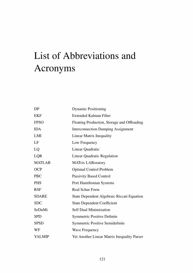
List of Abbreviations andAcronyms
DP Dynamic Positioning
EKF Extended Kalman Filter
FPSO Floating Production, Storage and Offloading
IDA Interconnection Damping Assignment
LMI Linear Matrix Inequality
LF Low Frequency
LQ Linear Quadratic
LQR Linear Quadratic Regulation
MATLAB MATrix LABoratory
OCP Optimal Control Problem
PBC Passivity Based Control
PHS Port Hamiltonian Systems
RSF Real Schur Form
SDARE State Dependent Algebraic Riccati Equation
SDC State Dependent Coefficient
SeDuMi Self Dual Minimization
SPD Symmetric Positive Definite
SPSD Symmetric Positive Semidefinite
WF Wave Frequency
YALMIP Yet Another Linear Matrix Inequality Parser
121

122

Summary
Dynamic positioning (DP) refers to maintaining the position and heading of a seavessel under specified limits by exclusively using thrusters and propellers. This
was usually achieved by using conventional techniques like anchoring and mooring,until the late sixties. Since then more sophisticated DP systems are being used fordynamic positioning.
A DP system consists of three main units: a power system, a DP control system,and a thruster system. A vessel whose motion is controlled by DP system is called aDP vessel. With the fast growing offshore industry, the demand for more accurate andstable DP systems has increased to ensure safety of the DP operations.
The focus of this research is the control system design for DP vessels. Startingpoint of the study of the DP control system design is a mathematical model of the seavessel. Two motion components of the vessel motion in sea are distinguished: a lowfrequency (LF) motion component and a wave frequency (WF) motion component.The LF motion is due to the slowly varying forces and moments due to the controlactions, waves, wind, and sea currents. The WF motion is caused by the first orderwave-induced wave loads. The measurement signal from the sensors (GPS and gyro)essentially contains both motion components.
An important consideration in the control system design for many dynamic posi-tioning problems is to compensate only the LF motion of the vessel. This is to avoidunnecessary wear and tear of the propulsion units. As the measurement signal playsan important role in the control design procedures, filtering of the WF componentfrom the measurement signal is essential so that only the LF component is transmittedto the controller. This problem of separating the LF motion component from the WFmotion component is called wave filtering.
An important aspect of control system design is its stability. In this thesis, wefirst study the local and the global aspects of the asymptotic stability of the DP vessel.The vessel model, we consider in this thesis, is nonlinear. This nonlinearity is dueto a single state variable which represents the heading angle of the vessel. The so-called state dependent coefficient (SDC) parametrization will transform the nonlinearvessel model into a pseudo-linear form with the system matrix being a function of theheading angle.
Some results on the global asymptotic stability studies of similar systems are reca-pitulated. Then we discuss two counterexamples to analyze the sufficient conditions
123
124 Summary
for the global asymptotic stability of the pseudo-linear system. In the first counterex-ample, we consider a system matrix which is a function of a single state component.We show that it is continuous, Hurwitz, and exponentially bounded. We further showthat these conditions are not sufficient to establish global asymptotic stability of thecorresponding pseudo-linear system. In the second counterexample, in addition tothe above mentioned set of conditions for the system matrix, we also assume thatthe system matrix is periodic in the single state component. We show that this stilldoes not lead to the set of sufficient conditions for global asymptotic stability of thepseudo-linear system.
For the case of a periodic dependence of the system matrix on a single state com-ponent, we propose a technique to prove the global asymptotic stability of the pseudo-linear system. This technique is a combination of the linear matrix inequalities (LMIs)and the Lyapunov stability theory. We use this technique to prove the global asymp-totic stability of the nominal (all the external disturbances are known or there are nodisturbances) vessel model with a naive state feedback controller in Chapter 3 andwith the Riccati equation based controller in Chapter 4.
In this thesis, the so-called state dependent algebraic Riccati equation (SDARE)technique is used to address the regulation problem of the DP vessel. We start with anominal case when there is no WF motion involved and measurements are noise free.The SDARE control design is used to regulate the vessel to the desired equilibriumposition. We then proceed with the so-called nonnominal case in which the distur-bance vector is unknown and the measurements also contain noise. The disturbancevector is modeled as a first order Markov process. Therefore, the disturbance vectorcan be concatenated with the state of the vessel model.
The SDARE control design is a state feedback method. Therefore, knowledgeof the entire state of the system is required. The output equation in the model ofthe DP vessel indicates that only the noisy position and heading measurements areavailable for feedback. Therefore, an observer is required to estimate the completestate of the system. The pseudo-linear SDARE observer is used to get these stateestimates. We conclude the SDARE control design concept by taking into account theWF component in the measurement model. In this case, the noisy measurements arecontaminated with the WF component as well, which requires wave filtering. We usethe SDARE technique to address the estimation and filtering problems. Simulationexperiments performed by using the data of a supply vessel have shown good resultsas far as the performance of the SDARE controller and observer is concerned.
We present the Fourier series interpolation (FSI) method which reduces the com-putation time of the algebraic Riccati equation. The effectiveness of the FSI methodis shown in the SDARE approach for the DP control system design. This is especiallyuseful in situations where the solution of the SDARE is required online. The fastcomputation of the SDARE may be required in the cases when this technique is usedwith systems whose dynamic response is fast/high. The idea of the method discussedin this thesis is limited to the special case of the SDARE whose coefficient matricesdepend on a single state component in a periodic way. The underlying idea behind thereduction in computation time of the solution of the SDARE is the offline computationof the Fourier coefficients which effectively reduces the online computations.
The regulation problem of the DP vessel is also addressed by using the port-Hamiltonian formulation. In this context, we study only the control design problem.

Summary 125
The estimation and wave filtering are assumed to be addressed separately and wemove on from this point to address the control design problem. The interconnectiondamping assignment passivity based control (IDA-PBC) design technique is used tointroduce two control laws: the classical IDA-PBC design and the extended IDA-PBCdesign. The former controller provides the desired performance in the nominal casebut it fails to stabilize the system at the desired location in presence of unknown ex-ternal disturbances. To address this bottleneck in the design, the extended IDA-PBCdesign is introduced to yield the desired performance.
There are two notable features in the port-Hamiltonian based study of the DPproblem. The first one is that there is an additional degree of freedom in the form of theHamiltonian (also sometimes referred to as the energy of the system) function whichhelps in improving the performance and analysis of the controller. The second featureof the port-Hamiltonian formulation is that it offers the freedom to add additionaldamping through the controller action which helps in improving the performance ofthe controller and it simplifies the tuning of the gains.
To explain the effects of the Hamiltonian formulation on the performance of thecontroller, we consider two different formulations of the Hamiltonian function: aquadratic and a trigonometric. Simulation results have revealed that each formulationgives a different heading angle profile of the vessel in cases when the initial headingangle is above π radians. The profile corresponding to the trigonometric formula-tion gives the optimal heading angle profile. The effect of additional damping is alsoexplained by a simulation result.
In conclusion, the search for the sufficient conditions for global asymptotic sta-bility of the pseudo-linear systems with state dependency of the system matrix on asingle state component, is still open for further research. The DP problem has a widerange of issues associated with it. This study is mainly focussed on the regulation ofthe DP vessel to a desired equilibrium point. The ideas and techniques introduced inthis dissertation can be employed also to study various other DP problems like pathfollowing, trajectory tracking, etc. The study of the port-Hamiltonian framework forfiltering and estimation problems of the DP vessel also remains an interesting andchallenging research problem.

126

Samenvatting
Dynamisch positioneren (DP) is een term uit de scheepvaart die betrekking heeftop het regelen van de positie en behouden van de koers van een vaartuig, binnen
voorgeschreven grenzen en uitsluitend door middel van boegschroeven en propellers.Tot in de tweede helft van de zestiger jaren werd dit voornamelijk gedaan door conven-tionele technieken, zoals verankering en meertrossen. Sindsdien is men gaandewegovergegaan op complexere DP systemen.
Een DP systeem omvat drie hoofdbestanddelen: een stroomvoorzieningssysteem,een DP regelsysteem, en een boegschroef systeem. Een DP vaartuig is een vaartuigwiens sturing wordt geregeld door een DP systeem. Dankzij de snelle groei van deoffshore industrie, stijgt de vraag naar nauwkeurigere en stabielere DP systemen diede veiligheid van DP operaties waarborgen.
In dit onderzoek ligt de nadruk op het regelsysteem voor DP vaartuigen. Hier-toe moet allereerst een mathematisch model van het vaartuig worden gemaakt. Debeweging van een vaartuig op zee kan worden opgesplitst in twee componenten: eenlage golffrequentie (LF) component en een hogere golffrequentie (GF) component. DeLF component wordt veroorzaakt door de traag veranderende krachten en momentendoor de regeling, en door golven, wind, en zeestromingen. De WF component wordtveroorzaakt door de impact van eerste orde golven. Deze twee componenten kunnenworden reconstrueerd uit het meetsignaal van de bewegingssensoren (GPS en gyro).
Een belangrijk aspect van het ontwerp van een DP regel systeem is dat men bijvoorkeur alleen wil anticiperen op de LF component van de beweging. Dit voorkomtonnodig gebruik (en dus slijtage) van de propellers. Daarom is het van belang om zonauwkeurig mogelijk de WF component uit het meetsignaal te filteren. Dit probleemwordt wave filtering genoemd.
Stabiliteit is een belangrijk aspect van een regelsysteem. In dit proefschrift beschouw-en we zowel lokale als de globale asymptotische stabiliteit van een DP vaartuig.Het mathematische model voor een vaartuig is niet-linear. Het niet-linear zijn wordtveroorzaakt door een toestandsvariabele die de koershoek van het vaartuig beschrijft.Door middel van een zogenaamde toestands-afhankelijke coefficienten parameteriza-tie (SDC parametrization) kan het niet-lineare stelsel worden omgeschreven in eenpsuedo-lineair stelsel, waarvan de systeem matrix een functie is van de koershoek.
Enkele resultaten betreffende globale asymptotische stabiliteit worden in dit proef-schrift kort samengevat. Vervolgens bespreken we een tweetal tegenvoorbeelden die
127
128 Samenvatting
informatie verschaffen over voldoende voorwaarden voor globale asymptotische sta-biliteit van het pseudo-lineaire systeem. Het eerste tegenvoorbeeld betreft een sys-teemmatrix die afhangt van een toestandsvariabele. We laten zien dat deze systeem-matrix continu, Hurwitz, en exponentieel begrensd is. Echter, dit blijkt niet voldoendevoor globale stabiliteit van een desbetreffende pseudo-lineair systeem. Ons tweedetegenvoorbeeld toont aan dat, als naast de bovengenoemde eigenschappen van de sys-teemmatrix ook nog wordt aangenomen dat deze periodiek is, dit nog steeds niet hoeftte leiden globale asymptotische stabiliteit.
Voor het geval dat de systeemmatrix periodiek afhangt van een variabele, wordteen aanpak geponeerd die geschikt zou kunnen zijn om de globale asymptotische sta-biliteit van het systeem aan te tonen. Deze aanpak is gebaseerd op een combinatie vanlineaire matrix ongelijkheden (LMIs) en de Lyapunov stabiliteits theorie. Wij passendeze aanpak toe om de globale asymptotische stabiliteit aan te tonen van een nomi-naal vaartuigmodel met twee verschillende regelingen: In hoofdstuk 3 beschouwen weeen naive state feedback regelsysteem, en in hoofdstuk 5 een regelsysteem gebaseerdop de Riccatti vergelijking. Een nominaal vaartuigmodel is een model waarbij alleeventuele externe verstoringen bekend worden verondersteld.
In dit proefschrift wordt de regeling van het DP vaartuig gerealiseerd met behulpvan de zogenaamde toestandsafhankelijke algebraısche Riccatti vergelijking (SDARE).We beginnen met het eenvoudige geval dat er geen sprake is van een WF beweg-ingscomponent en het meetsignaal geen ruis bevat. We gebruiken het SDARE regel-systeem dat een vaartuig in de gewenste evenwichts positie brengt. We vervolgenons onderzoek door het geval te beschouwen dat de verstoringsvector onbekend is enhet meetsignaal ruis bevat. De verstoringsvector wordt gemodelleerd door een eerste-orde Markov process. Het gevolg daarvan is dat de verstoringsvector ingebracht kanworden in de toestand van het vaartuig.
Het SDARE regelsysteem is een feedback systeem. Daarom is het nodig beschikk-ing te hebben over de toestand (positie, richting) van het systeem. Echter, de vergeli-jking met behulp waarvan de positie en richting van een DP vaartuig kan wordenbepaald, bevat ruis. Daarom moet een waarnemer worden ontworpen die de daadw-erkelijke toestand en richting schat. De pseudo-lineaire SDARE observer is gebruiktom deze schattingen te maken. Als laatste toevoeging aan het ontwerp van het SDAREregelsysteem wordt het effect van de WF bewegingscomponent meegenomen. In ditgeval moet uit de meetsignalen met ruis ook nog de WF component worden gefilterd.We gebruiken de SDARE teckniek om de ruis en de WF component weg te filteren.Simulaties op basis van de data van een bestaand vaartuig laten zien dat de SDAREregelaar en waarnemer goed presteren.
We presenteren de Fourier reeks interpolatie (FSI) methode, die de rekentijd voorhet oplossen van de algebraische Riccati vergelijking verkort. Deze methode blijkteffectief voor de SDARE aanpak van het ontwerp van een DP regelsysteem. In het bi-jzonder is de aanpak nuttig als de oplossing van SDARE online nodig is. De snelheidvan SDARE kan nodig zijn in systemen waarvan de dynamische response hoog/snel is.In dit proefschrift bestuderen we deze aanpak slechts voor SDARE waarvan de coeffi-cient matrices afhangen van een toestandscomponent, en wel op een periodieke wijze.Het achterliggende idee van de reductie in rekentijd van de oplossing van SDARE isdat de Fourier coefficienten offline bepaald worden, hetgeen de rekentijd van de onlineberekeningen effectief reduceert.

Samenvatting 129
Naast SDARE beschouwen wij ook de port-Hamiltoniaanse formulering voor hetregelsysteem van een DP voertuig. In deze context beschouwen we alleen het ontwerpvan de regelaar. Wij presenteren dus geen aanpak voor het filteren van de ruis en deWF component. Voor de regelaar gaan wij uit van de interconnection damping as-signment passivity based control (IDA-PBC). Hierbij maken we verschil tussen hetklassieke IDA-PBC ontwerp en het uitgebreide IDA-PBC ontwerp. Het klassieke on-twerp leidt tot een goed gedrag bij het nominale geval. Echter, indien er onbekendeexterne verstoringen zijn, is het systeem met een klassieke IDA-PBC niet stabiel. Deuitgebreide IDA-PBC heeft dit probleem niet.
De port-Hamiltoniaanse aanpak van het DP probleem heeft twee aantrekkelijkeeigenschappen. Ten eerste is er een extra vrijheidsgraad in de vorm van de Hamiltoni-aan (ook wel de energie van het systeem genoemd). De tweede aantrekkelijke eigen-schap van de port-Hamiltoniaanse aanpak is dat het de mogelijkheid biedt een extrademping aan de acties van de regelaar toe te voegen. Beide eigenschappen verbeterende prestaties van de regelaar, en de tweede eigenschap vereenvoudigt het afstellen.
Wat betreft de keuze van de Hamiltoniaan beschouwen wij twee verschillende for-muleringen: een kwadratische en een trigonometrische Hamiltoniaan. Uit simulatiesis gebleken dat de twee methoden ieder een ander koersprofiel geven van het vaartuigals de initiele koers meer dan π radialen is. Het profiel horende bij de trigonometrischeformulatie geeft het optimale profiel. Het effect van extra demping wordt geanalyseerdmet behulp van een simulatie.
Kort samengevat is de zoektocht nog open betreffende een algemene voldoendevoorwaarde voor globale asymptotische stabiliteit van een pseudo-linear systeem waar-van de systeemmatrix middels een enkele parameter van de toestand afhangt. Het on-twikkelen van een DP systeem brengt veel uitdagingen met zich mee. Dit proefschriftbeschouwt in eerste instantie of een regelsysteem van een DP voertuig het vaartuig ineen gewenst evenwicht kan brengen. De ideeen en technieken die in dit proefschriftzijn ontwikkeld kunnen ook worden gebruikt om andere DP gerelateerde problemente bestuderen, zoals het volgen en bijhouden van de koers. Een ander interessant enuitdagend onderzoeksprobleem blijft het ontwikkelen van een filter voor ruis en voorde WF component in het port-Hamiltoniaanse framework.

130
Acknowledgments
Iam immensely elated to write the acknowledgments for my thesis. It is the culmina-tion of my PhD research and an end to my formal student life. It all started almost
30 years ago from a far-flung, two-room primary school in my native village Dhurnal.Starting from a school which still doesn’t have electricity, I had never thought thatone day I would end my student life by completing a PhD from a university like TUDelft. This long journey was not a stroll. There were many ups and downs. Therefore,first of all, I express my utmost gratitude to Almighty Allah who helped me to remainsteadfast and made it possible for me to complete a PhD from one of the world’s besttechnical universities, after such a humble start.
I especially thank my supervisor Jacob and promoters Geert Jan (my promoter forfirst two years of my PhD) and Arnold (my promoter till the end of my PhD). I wish toextend my profound thanks to Jacob and Geert Jan for providing me the opportunityto join TU Delft as a PhD student in the mathematical system theory group. I thankArnold, Geert Jan, and Jacob for their persistent confidence and trust in me. Theyalways motivated and encouraged me in times of doldrums and stagnation during myPhD research. They provided me with many opportunities to improve my scientificand professional skills by sending me to many scientific events during my tenure asa PhD student. I thank Arnold and Jacob for several reviews of my thesis draft andgiving useful feedback which helped me to improve its contents and presentation.
My primary interaction was with Jacob. He has been very supportive, candid,helpful and patient throughout my stay in Delft. We had numerous productive anduseful discussions. I learnt a lot of professionalism from him, of which this thesis isjust a subset. He provided me annual breaks to visit my family which really helpedme and my family. Thank you Jacob for all these favors and your help.
This part of acknowledgment is not complete without mentioning the warm hos-pitality and honor that Geert Jan, Elke, Jacob and Yvon have given to my wife andchildren when they came to the Netherlands. Especially, I admire the amiable andfriendly nature of Elke and Yvon: amazingly my kids became their intimate friends inone meeting.
I would like to express my gratitude to Dori, Evelyn, Dorothee, and Cindy for theirkind support in various office matters and related documentation at the departmentduring my PhD tenure. Most of my contact was with Dori. She is a wonderful person.Her interaction with colleagues is very passionate, like a mother I would say. She
131

132 Acknowledgments
made me feel at home! Many thanks to Dori and Dorothee for arranging wonderfuldays out with DIAM.
Special thanks to Carl and Kees for their support in Windows- and Linux- relatedissues. They were always around when I needed them. They were always kind toanswer my silliest questions! Thank you for making my computers function smoothly.
I would like to appreciate the assistance provided by Nuffic and CICAT. I wouldlike to thank Mrs. Minkman (and her colleagues) for the smooth dispersal of themonthly stipend which made my stay in the Netherlands free from any financial is-sues. Franca Post from CICAT deserves special thanks from me, my wife, and mychildren for her contribution in our family reunion in Delft. Those were the best daysduring my stay in the Netherlands and Franca deserves the credit for providing us withthose joyous moments. Besides this extraordinary occasion, she helped a lot in variousoffice matters and related documentation. Thank you Franca!
I shared an office with many people. I thank Katerina, Diana, Adolfo, Arnau,Evans, Jeroen, Jonas, Yusef, and Saeeda for being supportive, accommodating, andcheerful officemates. Katerina was my first colleague in TU Delft. She deserves myexclusive acknowledgment for providing me a lot of help in difficult times in the earlyphase of my PhD life. Katerina, I still fondly remember your frequently used amusingphrases:“I am disappearing slowly”, “Was somebody looking for me?”, “Am I dis-turbing you!”, “Sorry, talking to myself!”. Arnau also deserves special recognition.He helped me a lot with putting my PhD on track. His arrival at DIAM was a blessingfor me. He provided the catalyst for my PhD process. I wish both Katerina and Arnauthe very best in their lives!
I would like to express appreciation for all people from the probability and riskanalysis group, analysis group, and optimization and system theory group for provid-ing a wonderful working environment. It was a pleasure to be a part of this friendlymilieu. Thank you for all the smiles and greetings!
My special thanks goes to Eddie Kim for reading my thesis and English propo-sitions. Thank you Eddie for helping me in improving the text and presentation. Healso deserves special appreciation for being a lively and wonderful person.
I would like to thank Prof. Jan van Schuppen for his time and interest in readingmy thesis. Thank you Jan for many useful discussions and remarks about my research.
I thank Sonja Cox for sparing her precious time and helping me with the Dutchsummary of my thesis and the Dutch translation of my thesis propositions. I appreciateher friendly and very supportive disposition.
I would like to thank the Dutch Society in general. I really enjoyed my stay inthe free and open environment. People really respect each other irrespective of race,religion, and appearance. People are very friendly and supportive although they arevery reserved in general. It was a pleasure and a great learning experience for meduring my stay in the Netherlands. I really like the way people greet each other.
I appreciate the Ima’ms and the committee of Masjid Sultan Ahmet for their hos-pitality and care during the months of Ramadhan. The iftar arrangements were a greatfacility and comfort for students in Delft. The presence of a sizable Muslim commu-nity in Delft was a great source of convenience in many aspects.
Hisham, Mehfooz, and Zubair deserve special mention for their help on my initialarrival in Delft. They really ensured that I would not face any trouble being new inDelft. I had a long stay in Delft spanning over 5 years. I lived with many persons dur-

Acknowledgments 133
ing my stay in Delft. I appreciate and commend Haleem, Hamayun, Raghu, Sidharth,Iftikhar Faraz, Asim, Khaled, Ibrahim, and Hanan for their support, patience, and ver-satile and pragmatic company. You all made my stay in Delft cozy and comfortable.
My heartiest thanks go to Hanan for many delicious and generous dinners andfood. Hanan, you really saved me from starving! I never met such a jolly and gen-erous Sheikh and would not meet again. Keep it like that and try being a bit moreresponsible! I would like to thank Iftikhar Faraz for his kind hospitality and help onnumerous occasions! I would like to extend my gratitude to Ibrahim for his kind scold-ings and for motivating me to memorize the recitation of surah Al-Rehman. Words ofthanks go to Faisal Nadeem for being a frank and a dependable friend, helping me onvarious occasions, sharing gossip, and numerous discussions on cricket! I would liketo thank Tariq Abdullah for being a supportive and caring neighbor during my stay inthe Vrijenban region of Delft.
Nadeem deserves a special mention for arranging weekly study circle gatheringsof compatriots in Delft. I always enjoyed those meetings. I learned many new things.All those who used to take part in those meetings deserve special thanks for makingthem useful and productive.
I was lucky to have so many Pakistanis around during my stay in Delft. This wasa great blessing! Life became very easy due to useful information sharing and givingone another small favors. Generally, people were friendly, social, and supportive. Wehad many memorable social events and get togethers. I would like to extend my thanksto all those who provided opportunities to enjoy Pakistani food from time to time. Wehad a good cricket team and we enjoyed playing together.
I would also like to mention my Indian friends here. It was here in the Netherlandsthat I met an Indian national for the first time. I am really amazed by their modestyand friendly nature in general. We enjoyed good times playing cricket and had a lotof fun! Special thanks to Navin and Amol for their time and useful discussions aboutmy research.
A word of thanks goes to Dr. Ata ur Rehman for his brainchild which revolution-ized the higher education sector in Pakistan. I would also like to thank the HigherEducation Commission of Pakistan, the government, and the people of Pakistan whoall made it possible for me to come and stay in the Netherlands to pursue PhD studies.
There are many people in Pakistan who helped and encouraged me in difficulttimes during my stay in the Netherlands. They made it possible so that I wouldn’thave any problems back home in Pakistan which allowed me to be focussed withmy job in Delft. My mother, brothers and sisters, and in-laws of my sisters have allsupported me well in their capacity. Especially, my youngest brother Rizwan andmy bhabhi Rehmat deserve very special recognition for being very supportive. Thefamily of my wife deserves special acknowledgments for being caring and supportiveto my family in my absence. My special thanks goes to my cousins Khalda and AbdulKhaliq, my aunts Mehr Bibi and Saeeda, Uncles Abdul Latif, Said Ahmad, and Yasin(and his family), friends, and relatives who supported me from time to time. Some ofthem really deserve more recognition but I am sorry for being brief here.
My late father, Dil Kabeer, who is unfortunately not with us today deserves veryspecial recognition. It was his dream to see his children becoming successful in theirlives. He sacrificed his leisures to provide a good education to his children. I haveno doubt that he would have been the happiest person in the world at the success-

134 Acknowledgments
ful completion of my PhD. Abbu! This work is a small token for your struggle andsacrifices!
Now I come to the most difficult and important part of this acknowledgment! It’shard for me to describe in words the role of my wife and kids during my PhD studies.They deserve very special appreciation for their patience and endurance during mylong and protracted PhD stint. I always received a lot of motivation and inspirationfrom my wife whenever I got tired from research. The gleaming eyes and smilingfaces of my kids always provided me great vigor in listless moments. On one hand itwas a tough time for all of us but on the other hand it was a great learning experienceas well. We realized the value and importance of many things which will help us infuture life. I applaud my wife for her pristine love, good work in running the familyaffairs and raising the children excellently in my absence. I am happy that the testingtime is going to end soon with a fruitful outcome. It’s carnival time for all of us. I amraring to see you all and to spend more time with you! I wish and pray for a happyand peaceful future with you all!
A word of thanks goes to myself for enduring all stress and fatigue. There werehardly any serendipitous moments in the last 5 years. But on a positive note, I shouldnot forget the experiences gained and promises made to myself during these years.Now it’s time to pay attention to things which I put off due to PhD priorities.
To the readers of this acknowledgment page, I want to share a personal experience.When you decide to do anything in life, you will do it for sure, sooner or later. Itdepends upon your determination and focus. Never give up!
Finally, I thank the members of my promotion committee for devoting some oftheir precious time to scrutinize my thesis, and I acknowledge those committee mem-bers who traveled to Delft for the public defense of this dissertation. Thank you allvery much for your time and interest. Thank you for reading my work with interestand all the insightful feedback!
–The End –
QmÌ'@ AK.
IÜ
ß
Shah Muhammad YÒm× èA
March 22, 2012 2012 h PAÓ 22

Publications
SHAH MUHAMMAD AND JACOB VAN DER WOUDEA counter example to a recent result on the stability of nonlinear systems, IMA Jour-nal of Mathematical Control and Information. Vol. 26, No. 3, August 2009, pp 319-323.
SHAH MUHAMMAD AND JACOB VAN DER WOUDEThe Fourier Series Interpolation (FSI) Method for the Solution of the SDARE. Inproceedings of the UKACC International Conference on Control (CONTROL 2010),September 7-10, 2010, Coventry, UK.
SHAH MUHAMMAD AND ARNAU DORIA-CEREZOOutput Feedback Passivity-based Controllers for Dynamic Positioning of Ships. InProceedings of the 14th Edition of the Dynamic Positioning Conference (DP CON-FERENCE 2010), October 12-13, 2010, Houston, USA.
SHAH MUHAMMAD AND JACOB VAN DER WOUDEOn stability conditions for systems with periodic state dependent coefficients, IMAJournal of Mathematical Control and Information. Vol. 28, No. 1, March 2011, pp 97-102.
SHAH MUHAMMAD AND ARNAU DORIA-CEREZOPassivity Based Control Applied to the Dynamical Positioning of Ships. To appear inIET Journal of Control Theory and Applications.
135

136
Curriculum Vitae
Shah Muhammad was born on the 6th of January, 1977 in Talagang, Pakistan. He gothis primary and secondary education mainly from government schools and colleges inhis native town. He completed his B.Sc. in 1997 from the University of the Punjab andsubsequently he earned an M.Sc. in Mathematics from Islamia University Bahawalpurin 1999 with distinction. Later on he worked as a Scientific Officer for four years inGhulam Ishaq Khan (GIK) Institute of Engineering Sciences and Technology, Topi,Pakistan. This stint ended on June 30, 2005. Since September 2006, he has been in theNetherlands, pursuing his PhD in the Mathematical System Theory and Optimizationgroup at the Delft Institute of Applied Mathematics, Delft University of Technology.
He has presented several papers during his PhD studies in various seminars andconferences related to dynamical systems and control theory. Prominent activitiesinclude his participation and presentation in the 1st Elgersburg School on Mathemati-cal Systems Theory, organized by Technische Universitat Ilmenau on March 30-April3, 2009 in Elgersburg, Germany, the Benelux meetings on systems and control (2009and 2010 editions), the UKACC Conference on Control held in Coventry, UK in 2010,and the 2010 DP Conference held in Houston, USA. He has also reviewed scientificarticles in his field. He has two published and one accepted journal article.
Sports and reading formed Shah’s extra-academic activities during his student life.At Islamia University Bahawalpur, he won first prize in the 5 Km long distance raceand ended up third in the 1500 m race. He is a good player of cricket. He is a fluenttop order batsman who likes to play aggressively. He is also a very agile fielder andhas a very safe pair of hands anywhere in the outfield and in the slip cordon. Shahis a strong believer that sports are an indispensable part of an individual’s life and heintends to promote sporting culture among the masses and society as a whole.
Shah’s post PhD plans are to join a dynamic and growing organization or institutewhere he can use the knowledge and expertise acquired during his academic and re-search career. He likes to share and transfer his experience to prospective colleaguesand students. He believes that research culture is a key to solve the problems of dailylife and to overcome the challenges of the modern era. Shah intends to work for thepromotion of research culture, especially in the developing and third world countries.
137