Dynamic Volume-Return Relation of Individual Stocks�

Guillermo Llorente Roni Michaely Gideon Saar Jiang Wang

First version: November 15, 1997

Current version: August 15, 2000

Abstract

We examine the dynamic relation between return and volume of individual stocks. Using

a simple model in which investors trade to share risk or speculate on private informa-

tion, we show that returns generated by risk-sharing trades tend to reverse themselves

while returns generated by speculative trades tend to continue themselves. We test this

theoretical prediction by analyzing the relation between daily volume and �rst-order re-

turn autocorrelation for individual stocks listed on the NYSE and AMEX. We �nd that

the cross-sectional variation in the relation between volume and return autocorrelation

is related to the extent of informed trading in a manner consistent with the theoretical

prediction.

�Llorente is from Facultad de C. Economicas, Universidad Autonoma de Madrid, 28049 Madrid, Spain

(telephone: 34-91-397-4812, fax: 34-91-397-4091, and email: guiller@uam.es); Michaely is from the

Johnson School of Management, Cornell University, Ithaca, NY 14850 (telephone: 607-255-7209, fax: 607-

254-4590, and email: rm34@cornell.edu); Saar is from the Stern School of Business, New York University,

New York, NY 10012 (telephone: 212-998-0318, fax: 212-995-4233, and email: gsaar@stern.nyu.edu);

Wang is from the Sloan School of Management, MIT, Cambridge, MA 02142-1347 and the National

Bureau of Economic Research (telephone: 617-253-2632, fax: 617-258-6855, and email: wangj@mit.edu).

The authors thank I/B/E/S for providing the data on analysts' earnings forecasts, Yiming Qian for her

research assistance, and Juan del Hoyo, David Easley, Gustavo Grullon, John Heaton, Soeren Hvidkjaer,

Robert Jarrow, Andrew Lo, N. Nimalendran, Maureen O'Hara, Bhaskaran Swaminathan, seminar par-

ticipants at Cornell University, New York University, the 1998 Western Finance Association Meetings,

and a referee for helpful comments.

1 Introduction

Market participants carefully watch the volume of trade, which presumably conveys valu-

able information about future price movements. At the heart of the matter are the ques-

tions of why investors trade and how trades with di�erent motives relate to prices. Two

reasons are often mentioned for why investors trade: to rebalance their portfolios for risk

sharing and to speculate on their private information. These two types of trades, which

we call hedging and speculative trades, respectively, result in di�erent return dynamics.

For example, when a subset of investors sells a stock for hedging reasons, the stock's

price must decrease to attract other investors to buy. Since the expectation of future

stock payo� remains the same, the decrease in the price causes a low return in the cur-

rent period and a high expected return for the next period. However, when a subset of

investors sells a stock for speculative reasons, its price decreases, re ecting the negative

private information about its future payo�. Since this information is usually only partially

impounded into the price, the low return in the current period will be followed by a low

return in the next period, when the negative private information is further re ected in

the price. This example shows that hedging trades generate negatively autocorrelated

returns and speculative trades generate positively autocorrelated returns.

Intensive trading volume can help to identify the periods in which either allocational or

informational shocks occur, and thus can provide valuable information to market observers

about future price movements of the stock. In periods of high volume, stocks with a high

degree of speculative trading tend to exhibit positive return autocorrelation and stocks

with a low degree of speculative trading tend to exhibit negative return autocorrelation.

In this paper, we construct a simple equilibrium model to derive the return dynamics

generated when investors trade both to hedge and to speculate. The model illustrates

that the relation of current return, volume, and future returns depends on the relative

signi�cance of speculative trade versus hedging trade. If speculative trading in a stock is

relatively insigni�cant, returns accompanied by high volume tend to reverse themselves in

the subsequent period. If speculative trading in a stock is signi�cant, conditioned on high

volume, returns become less likely to reverse and can even continue in the subsequent

period. The di�erence in the relative importance of speculative trading among di�erent

stocks gives rise to the cross-sectional variation in their volume-return dynamics.

We empirically test the predictions of the model by analyzing the daily volume-return

dynamics of individual stocks traded on the NYSE and AMEX. The basic structure of the

empirical tests is as follows. For each stock in the sample, we use a time-series regression

1

to �nd the relation between current return and volume and future return. Then, guided

by the predictions of the model, we examine how this relation varies across stocks with the

extent of speculative trading. We consider several proxies, such as market capitalization

and bid-ask spread, for the degree of speculative trading across stocks. Consistent with the

model, we �nd signi�cant di�erences in the dynamics of returns and volume across stocks

with di�erent degrees of information asymmetry. Stocks of smaller �rms, or stocks with

higher bid-ask spreads, show a tendency for return continuation following high volume

days. Stocks of larger �rms, or stocks with smaller bid-ask spreads, show almost no

continuation and mostly return reversal following high-volume days.

We examine the robustness of our results along several dimensions. First, we explore

alternative econometric speci�cations of our tests and �nd that they do not change our

results. Second, we replace the daily interval with a measurement period that equates the

amount of noise trading across stocks, and show that it does not a�ect our �ndings. Third,

we check the sensitivity of our �ndings to the e�ect of the bid-ask bounce, which can also

cause return autocorrelation. We perform this check by repeating our main experiment

using returns calculated from mid-quotes rather than from the closing price of the day.

This alternative procedure does not alter our conclusions. Fourth, we show that our

�ndings are not sensitive to alternative de�nitions of trading volume. Fifth, in light of

recent papers that identi�ed a larger analyst following with a smaller adverse selection

problem, we use analyst following as an additional proxy for information asymmetry. Our

results show that stocks that are followed by more analysts exhibit less return continuation

following high volume days.

We also test the hypothesis that it is �rm-speci�c private information that a�ects

the cross-sectional variation in the dynamic volume-return relation. We decompose both

the volume and return series into systematic and unsystematic components. We �nd

that the relation between information asymmetry and the in uence of volume on the

autocorrelation of returns persists when we remove the market-wide variations from the

analysis.

Many recent papers investigate the relation between return dynamics and trading vol-

ume. Several of them focus on aggregate returns and volume (e.g., Campbell, Grossman,

and Wang, 1993 (henceforth CGW); Du�ee, 1992; Gallant, Rossi, and Tauchen, 1992;

and LeBaron, 1992). These studies �nd that returns on high-volume days tend to reverse

themselves.

A few studies also use returns and volume of individual stocks (e.g., Antoniewicz, 1993;

2

Conrad, Hameed, and Niden, 1992; Morse, 1980; Stickel and Verrecchia, 1994). In par-

ticular, Antoniewicz �nds that returns of individual stocks on high-volume days are more

sustainable than are returns on low-volume days. Stickel and Verrecchia �nd that when

earnings announcements are accompanied by higher volume, returns are more sustainable

in the following days. The results of these two papers, from pooling together individual

returns and volume, contrasts with the result from aggregate returns and volume. How-

ever, these studies do not provide an explanation that reconciles the two phenomena, nor

do they examine the cross-sectional variation in the volume-return relation among the

stocks.1

Our paper provides a model that reconciles the contrasting empirical results on the

volume-return relation at the aggregate and the individual levels. The model demonstrates

how these results are related to the cross-sectional variation in the volume-return relation.

Unlike CGW, we recognize information asymmetry as an important trading motive in

addition to risk sharing. We show that for stocks with low information asymmetry (like the

market indices and the big �rms studied by CGW and LeBaron, 1992), returns following

high-volume days exhibit strong reversals, as in CGW. However, for stocks with high

information asymmetry, returns following high-volume days exhibit only weaker reversals

or even continuations, which is consistent with the �ndings of Antoniewicz (1993) and

Stickel and Verrecchia (1994) who use pooled returns and volume of individual stocks.

Our analysis highlights the importance of information asymmetry in understanding the

dynamic volume-return relation and demonstrates the more general nature of this relation,

which was only partially captured by the aforementioned papers.

On the theoretical side, our model is very close to that of Wang (1994) but less com-

plex. Simpli�cation allows us to obtain sharper predictions on the dependence of a stock's

dynamic volume-return relation on the extent of information asymmetry, which we test

empirically. Our paper is also related to a paper by Blume, Easley, and O'Hara (1994),

which examines the informational role of volume. In their model, investors can extract

useful information from both volume and prices. In our model, volume provides no ad-

ditional information to investors. However, the dynamic relation between volume and

returns allows observers of the economy to better understand its underlying characteris-

1In a recent paper, Lee and Swaminathan (2000) show that past volume provides valuable information

about future returns over horizons of six months. By assigning stocks to portfolios based on past volume

and price changes, they show that using the prior six-months-volume in combination with price changes

is superior to using past price changes alone in predicting long term returns. Speci�cally, they show

that buying low-volume winners and selling past high-volume losers outperform a pure price momentum

strategy. The nature of their result is similar to that of Antoniewicz (1993), but at a longer horizon.

3

tics, such as the degree of information asymmetry, which is our focus.

Other related papers include Brown and Jennings (1989) and Grundy and McNichols

(1989). In particular, Brown and Jennings examine the characteristics of return auto-

correlations when investors trade on private information. They do not consider volume,

which is partially exogenous in their model due to the presence of noise traders. We focus

on the joint behavior of return and volume because it provides more information about

the underlying economy.2

On the empirical side, our paper is related to Hasbrouck (1988, 1991) who utilizes

transactions data to examine the impact of trades on prices and quotes. He uses a

linear empirical model to capture how such an impact might be related to the inventory

control of specialists and to the private information behind trades. Even though we do

not focus on the actual trading process, in many ways our paper deals with the same

issues, namely, how trades with di�erent motives generate di�erent return dynamics.

Nonetheless, our paper is di�erent in several ways. First, while Hasbrouck's analysis is

based on heuristic linear speci�cations, our analysis is based on a theoretical model, which

leads to a particular non-linear speci�cation. Second, Hasbrouck's analysis conditions on

a trade's direction, relying on a heuristic algorithm to infer its direction from publically

available data. We prefer to use volume that is not subject to errors introduced by trade

classi�cation algorithms. Third, our analysis focuses on the cross-sectional di�erence

among stocks.

The paper proceeds as follows. Section 2 presents the model and the theoretical

predictions that we test. Section 3 describes the empirical methodology and Section 4

provides our empirical results. Section 6 concludes. All proofs are contained in the

Appendix.

2 The Model

In this section, we present a model of the stock market in which investors trade for both

allocation and information reasons. We use the model to show how the dynamic relation

between return and volume depends on the information asymmetry between investors.

Since our goal is to establish this dependence and to illustrate the economic forces behind

2It should also be noted that many theoretical papers in market microstructure deal with the impact

of private information on asset prices (e.g., Easley and O'Hara, 1987; Glosten and Milgrom, 1985; Kyle,

1985). However, the assumption of a competitive market maker in these models makes prices follow a

martingale, eliminating richer dynamics.

4

it, we keep the model as parsimonious as possible. We discuss possible generalizations of

the model toward the end of the section.

2.1 Economy

The economy is de�ned on a discrete time sequence, t = 0; 1; 2; : : : . There are two traded

securities, a riskless bond and a stock. The bond is in unlimited supply at a constant,

non-negative interest rate, r. The stock pays a dividend Dt+1 in period t + 1, which

consists of two additive components:

Dt+1 = Ft +Gt: (1)

Shares of the stock are traded in a competitive stock market. Let Pt denote the ex-

dividend price of the stock at time t.

There are two classes of investors, 1 and 2, with relative population weight of ! and

1 � !, respectively. Investors are identical within each class, but are di�erent between

the classes in their endowments and information. For convenience, an investor in class i

is referred to as investor i, where i = 1; 2.

Each investor is initially endowed with �x shares of the stock. He is also endowed with

a ow of income from a nontraded asset. In period t, investor i has Z(i)t units of the

nontraded asset that pays Nt+1 per unit in the subsequent period.

At time t, all investors observe the current dividend of the stock (Dt), its price (Pt), the

current payo� of the nontraded asset (Nt), and their own endowment of the nontraded

asset (Z(i)t for investor i). They also observe Ft, the forecastable part of each stock's

next-period dividend. In addition, class 1 investors observe Gt. Thus, they have private

information about future stock payo�s. The information set of investor i at time t is then

given by I(1)t = fD;P;N; F;G; Z(1)

g[0; t] and I(2)t = fD;P;N; F; Z(2)

g[0; t], where f�g[0; t]

denotes the history of a set of variables from time 0 to t.

Each investor maximizes expected utility over his wealth next period of the following

form:

E

��e��Wt+1

����I(i)t

�(2)

where � > 0 is the risk-aversion parameter.

All shocks (i.e., fFt; Gt; Nt; Z(1)t ; Z

(2)t 8 tg) are assumed to be normally distributed

with zero mean and constant variances: �2Ffor Ft, �

2Gfor Gt, �

2Nfor Nt, and �

(i)Z

2 for Z(i)t ,

respectively, where i = 1; 2. Furthermore, they are assumed to be mutually independent

5

(contemporaneously and over time), except for Dt and Nt, which are correlated with

E[DtNt] = �DN . In addition, for convenience in exposition, we set the riskless interest

rate at zero and each investor's initial endowment of stock shares at zero (�x = 0). (Thus,

the total supply of the stock is zero.) Without loss of generality, we set the investors' risk

aversion � at one.3

The model de�ned above captures two important motives for trading: allocation of

risk and speculation on future returns. Each investor holds the stock and the nontraded

asset in his portfolio. Since the returns on the two assets are correlated, as his holding of

the nontraded asset changes, each investor wants to adjust his stock positions to maintain

an optimal risk pro�le. This generates allocational trade in the model, which we refer

to as hedging trade.4 In addition, some investors might have private information about

future stock payo�s. As new private information arrives, they take speculative positions

in the stock in anticipation of high returns. This generates the informational trade in the

model that we refer to as speculative trade.

2.2 Equilibrium Price and Volume

Given a stock price process fPtg, the dollar return on one stock share is given by

Rt � Dt + Pt � Pt�1 (t = 1; 2; : : :) (3)

The return consists of two parts, a dividend and a capital gain. Let E(i)t [Rt+1] denote

investor i's conditional expectation of Rt+1 given his information at t, �(i)R

2 its conditional

variance, and X(i)t his stock holding. (Here, �

(i)R

2, the conditional variance of stock returns

for investor i, has no time subscript because it remains constant over time.) We have the

following proposition:

Proposition 1 The economy de�ned above has an equilibrium in which investor i's stock

holding is

X(i)t =

E(i)t [Rt+1]

�(i)R

2�

�DN

�(i)R

2Z

(i)t =

E(i)t [Dt+1]�Pt

�(i)R

2�

�DN

�(i)R

2Z

(i)t (i = 1; 2) (4)

3Our model, which uses Constant Absolute Risk Aversion preferences and normally distributed shocks,

exhibits homotheticity. That is, the implications of the model are invariant to proportional scaling of the

variances of all the shocks and the investors' risk aversion. Thus, it is convenient to express the results

to re ect this invariance. We choose to let � = 1 and thank the referee for suggesting this.

4Many papers have introduced nontraded assets to generate investors' hedging needs to trade in the

market. See, for example, Bhattacharya and Spiegel (1991) and Wang (1994).

6

and the ex-dividend stock price is

Pt = Ft + ~Pt � Ft + aGt �

�b(1)Z

(1)t + b(2)Z

(2)t

�(5)

where E(1)t [Dt+1] = Gt, E

(2)t [Dt+1] =

�~Pt � b(2)Z

(2)t

�and a, b(1), b(2), �

(1)R

2, �(2)R

2, and

are constants.

Each investor's stock holding has two components. The �rst component is proportional

to his risk tolerance and the risk-adjusted, expected stock return given his information.

This component re ects the optimal trade-o� between the return and risk of the stock.

The second component is proportional to the amount of his non-traded asset, and re ects

his need to hedge the non-traded risk.

The equilibrium stock price at time t depends on Ft and Gt, and on the amounts of

both investors' non-traded asset, Z(1)t and Z

(2)t , respectively. Ft gives the expected next-

period dividend based on (non-price) public information. Gt re ects class 1 investors'

private information on the next dividend. Z(1)t and Z

(2)t give the investors' need to use

the stock to hedge their nontraded risk.

An investor changes his stock position when there is a change in his expectation of

future stock returns or his exposure to nontraded risk. This generates trading in the

market. Given that trading is only between the two classes of investors, the volume of

trade, Vt, is given by the change in the total stock holdings of either class. Thus,

Vt = !jX(1)t �X

(1)t�1j = (1�!)jX

(2)t �X

(2)t�1j: (6)

2.3 Dynamic Relation Between Return and Volume

In our model, returns are generated by three separate sources: public information on fu-

ture payo�s, investors' hedging trades and their speculative trades. The returns generated

by di�erent sources exhibit di�erent dynamics.

Returns generated by public news on future payo�s are independent over time. As

public information about future dividends arrives (i.e., the realization of Ft at t), the

stock price changes to fully re ect the public information. As Section 2.2 shows, the price

change has no impact on investors' stock demands, despite changes in their wealth. As a

result, expected future returns remain unchanged. In other words, public news on future

payo�s results in a white noise component in stock returns.

Returns generated by trading are serially correlated. When investors trade for hedging

reasons, the stock price adjusts to attract other investors to take the other side. This

7

price change contains no information about the stock's future payo�s. Thus, a price

change generated by a hedging trade implies future returns of the opposite sign. For

example, when class 1 investors sell the stock to hedge their nontraded risk, the stock

price decreases, yielding a negative return for that period. However, the expected payo�

in the next period stays the same. Hence, the decrease in the price leads to an increase in

the expected return in the next period. Thus, returns generated by hedging trades tend

to reverse themselves.

When investors trade for speculative reasons, the price changes to re ect the informed

investors' expectation of the stocks' future payo�s. This expectation is ful�lled later on as

private information becomes public. Thus, a price change generated by speculative trade

implies future returns of the same sign. For example, when class 1 investors sell the stock

due to a negative signal on future stock dividends, the stock price decreases, yielding a

negative return for the current period. Since the price only partially re ects the private

information (in a non-fully revealing equilibrium), the return in the next period is more

likely to be negative as the private information becomes public. Thus, returns generated

by speculative trade tend to continue themselves.

The actual dynamics of returns depend on the relative importance of the three return-

generating mechanisms. We are interested in returns generated by trading, with particular

attention to the relative amount of hedging trade versus speculative trade and their rel-

ative impact on stock prices. By analyzing the serial correlation of returns generated by

trading among investors, we could learn about the relative importance of di�erent trading

motives. Therefore, we would like to separately identify the returns generated by trading

from those generated by public news on future payo�s, and examine their dynamics. We

use trading volume to facilitate this identi�cation. We observe that in our model, price

changes generated by speculative or allocational trading must be accompanied by high

volume, but those generated by public news about payo�s do not. In other words, by con-

ditioning on the current volume return pair, we can (imperfectly) identify trade-generated

returns. (See CGW for a discussion of this point.) Based on those returns, we can fur-

ther examine how they might predict future returns. When all trades are hedging trades,

current returns together with high volume predict strong reversals in future returns (as

shown in CGW). When speculative trades are more important, current returns together

with high volume predict weaker reversals (or even continuation) in future returns, as

suggested in Wang (1994).

To analyze more formally how the relative importance of hedging trade versus spec-

8

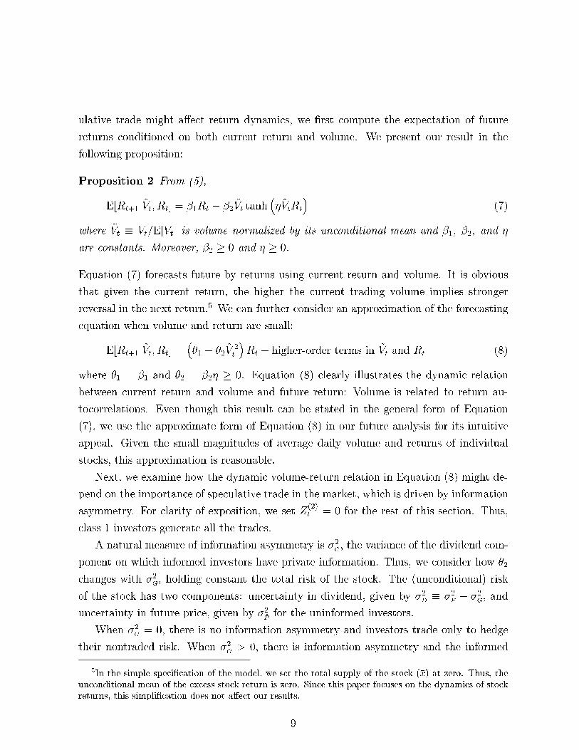
ulative trade might a�ect return dynamics, we �rst compute the expectation of future

returns conditioned on both current return and volume. We present our result in the

following proposition:

Proposition 2 From (5),

E[Rt+1j~Vt; Rt] = �1Rt � �2 ~Vt tanh

�� ~VtRt

�(7)

where ~Vt � Vt=E[Vt] is volume normalized by its unconditional mean and �1, �2, and �

are constants. Moreover, �2 � 0 and � � 0.

Equation (7) forecasts future by returns using current return and volume. It is obvious

that given the current return, the higher the current trading volume implies stronger

reversal in the next return.5 We can further consider an approximation of the forecasting

equation when volume and return are small:

E[Rt+1j~Vt; Rt] =

��1 � �2 ~V

2t

�Rt + higher-order terms in ~Vt and Rt (8)

where �1 = �1 and �2 = �2� � 0. Equation (8) clearly illustrates the dynamic relation

between current return and volume and future return: Volume is related to return au-

tocorrelations. Even though this result can be stated in the general form of Equation

(7), we use the approximate form of Equation (8) in our future analysis for its intuitive

appeal. Given the small magnitudes of average daily volume and returns of individual

stocks, this approximation is reasonable.

Next, we examine how the dynamic volume-return relation in Equation (8) might de-

pend on the importance of speculative trade in the market, which is driven by information

asymmetry. For clarity of exposition, we set Z(2)t = 0 for the rest of this section. Thus,

class 1 investors generate all the trades.

A natural measure of information asymmetry is �2G, the variance of the dividend com-

ponent on which informed investors have private information. Thus, we consider how �2

changes with �2G, holding constant the total risk of the stock. The (unconditional) risk

of the stock has two components: uncertainty in dividend, given by �2D� �2

F+ �2

G, and

uncertainty in future price, given by �2~P for the uninformed investors.

When �2G= 0, there is no information asymmetry and investors trade only to hedge

their nontraded risk. When �2G> 0, there is information asymmetry and the informed

5In the simple speci�cation of the model, we set the total supply of the stock (�x) at zero. Thus, the

unconditional mean of the excess stock return is zero. Since this paper focuses on the dynamics of stock

returns, this simpli�cation does not a�ect our results.

9

investors trade for hedging and speculative reasons. We then have the following proposi-

tion:

Proposition 3 For �2G= 0,

�2 = �20 ��2~P

��2D

=!2

�

�2DN�2Z

�2D

For �2G> 0 but small and holding �2

D, �2

~P constant,

�2 = �20

"1� !

1

�2D

+3

2�2~P

!#+ o

��2G

�(9)

which decreases with �2G.

Thus, holding constant the risk of the stock, �2 decreases with the degree of information

asymmetry between investors, which is measured by �2G.

Although this result is stated only for a small �2Gwhen an analytical proof is available,

we also examine its validity numerically when �2Gis large. By computing �2 for the

complete range of �G (between zero and �2D) for a wide range of parameter values (of �2

D,

�2Z, and �DN), we �nd that the dependence of �2 on �2

Gis always negative.6

Propositions 2 and 3 show how current return and volume predict future returns, and

how this predictability depends on the relative signi�cance of hedging trade versus spec-

ulative trade. In a cross-sectional context, all else equal, stocks with higher information

asymmetry will have lower �2 than will stocks with lower information asymmetry. It is

this dependence of the return-volume dynamics on the degree of information asymmetry

in the market, characterized in Equations (8) and (9), that we test empirically.

2.4 Discussion of the Model

Our model is similar to that of Wang (1994) with two simplifying assumptions. First,

shocks to the economy are independently (and identically) distributed over time. The

independence assumption implies that investors' private information is short-lived: It is

only about the next dividend, which is revealed after one period. Thus, the less-informed

investors do not have to solve the dynamic learning problem (and the corresponding

optimization problem for their stock demand), which simpli�es their policy.7 Second,

6Results of the numerical analysis are available upon request.

7For di�erent cases of long-lived private information in a competitive setting, see, for example, Brown

and Jennings (1989), Grundy and McNichols (1989), He and Wang (1995), and Wang (1994).

10

we assume that investors are myopic, which further simpli�es the investors' optimization

problem.

Our simpli�cation gives sharper results about the dependence of the volume-return

relation on information asymmetry, as shown in Proposition 3, while Wang (1994) relies

on numerical analysis and provides only examples. However, our model has the restrictive

implication that �2 remains non-negative even for high degrees of information asymmetry.

As shown in Wang (1994), when private information can be long-lived, �2 can become

negative as the degree of information asymmetry increases. In our empirical analysis, we

allow this possibility.

We assume that investors have constant absolute risk-aversion (CARA) and that assets

(the stock and the nontraded asset) have (conditionally) normally distributed payo�s.

The combination of these two assumptions allows closed form solutions for the model.

However, as a special feature of the CARA preferences, each investor's stock demand is

independent of his wealth. Hence, there is no income e�ect in investors' stock demand,

and public news on future asset payo�s (and the corresponding price change) does not

cause investors to trade in the market. Of course, for more general preferences, investors

do rebalance their portfolios in response to public news on future payo�s as their wealth

changes, giving rise to another motive for allocational trades. As mentioned earlier, our

model introduces a motive for allocational trade by including a set of nontraded assets in

investors' portfolio. We note that the detailed motive for allocational trades is not crucial

to our main result. This particular choice in the model is for tractability and simplicity.

Despite the simplifying assumptions of the model, it provides a clear illustration of

certain volume-return relations, which we believe to be more general than the model itself.

As discussed above, relaxing many of these assumptions is possible, but adds little to the

main thrust of the paper.8

3 Empirical Methodology

3.1 Data and Sample Description

Our primary sample comprises of all common stocks traded on the NYSE and AMEX.

From CRSP, we obtain data for daily return, price, number of shares traded and shares

8There are assumptions in the model that are more substantial, such as those on the preferences and

distribution combination and the information structure. Relaxing those would signi�cantly change the

model.

11

outstanding. We obtain quotes and bid-ask spreads data from the TAQ database. Our

sample period is from January 1st, 1993 to December 31st, 1998. We choose this six-year

sample period for two reasons. First, the TAQ database only starts at the beginning

of 1993. Second, the nature of our test requires that stock-speci�c parameters remain

constant over time, which may not be the case over a long period.9 During the sample

period, the CRSP database contains 3,538 stocks that were traded on the NYSE and

AMEX. To allow a more precise estimation of our time-series regressions, and a more

uniform cross-sectional comparison of the parameters, we further require that stocks in

the sample trade in at least two thirds of the days (1,000 days out of 1,516 possible trading

days). This requirement reduces our sample to 2,226 stocks.

Table 1 presents �rms' characteristics for the entire sample and for three subgroups

according to size. For each �rm i, we measure size (AvgCapi) as the average daily market

capitalization (number of shares outstanding multiplied by the daily closing price) over

the sample period. The market capitalization of �rms in our sample ranges from $3.61M

to $147.82B. As indicated by the columns 2 and 3 of the table, both the average daily

number of shares traded (AvgTrdi) and the average share turnover (AvgTurni), which is

the number of shares traded relative to shares outstanding, increase with �rm size. For

example, the daily average turnover is 0.27% for the Small size group and is 0.355% for

the Large size group. The average share price (AvgPrci in column 4) exhibits the same

pattern.

Using the data from TAQ, we construct a measure of a stock's bid-ask spread (BAsprdi).

In light of results in Madhavan, Richardson, and Roomans (1997), we use the opening

spread to capture the asymmetric information component of the spread. We then de-

�ne the relative spread for each stock as the average of the daily opening percentage

spread (opening bid-ask spread divided by the opening mid-quote) over the sample pe-

riod. Consistent with many prior studies, the relative spread is high for the Small size

group (4.11%), and decreases monotonically with �rm size (the average for �rms in the

Large size group is only 0.84%).

3.2 Return, Volume, and Proxies for Information Asymmetry

We use daily returns and trading volume to analyze the impact of information asymmetry

on the dynamic volume-return relation. The main reason to use daily data is to be able to

9In Section 4.2, we show that increasing the time horizon to ten instead of six years does not a�ect

our results.

12

relate our results to those of previous studies (e.g., Antoniewicz, 1993; CGW; LeBaron,

1992; and Stickel and Verrecchia, 1994).10 In Section 4.2 we consider an alternative

procedure to determine the appropriate time interval for our analysis empirically. The

return series we use for the estimation is the daily return of individual stocks from CRSP

(we test the sensitivity of our results to an alternative de�nition of returns that avoids

the potential bid-ask bounce problem in Section 4.3).

We use daily turnover as a measure of trading volume for individual stocks. We de�ne a

stock's daily turnover as the total number of shares traded in that day divided by the total

number of shares outstanding.11 Since the daily time series of turnover is nonstationary,

we measure turnover in logs and detrend the resulting series. To avoid the problem of

zero daily trading volume, we add a small constant (0.00000255) to the turnover before

taking logs.12 We detrend the resulting series by subtracting a 200-trading-day moving

average:

Vt = logturnovert �1

200

�1Xs=�200

logturnovert+s

where

logturnovert = log (turnovert + 0:00000255) :

Panel B of Table 1 provides summary statistics that describe the volume series used in the

estimation. While the �rst-order autocorrelation is higher for larger stocks, the pattern

becomes less pronounced in the �fth order and disappears in the tenth order. We test the

sensitivity of our results to alternative de�nitions of volume in Section 4.4.

As in CGW, we note that there is some slippage between the theoretical variables

in the model and those in the empirical part. Our model considers dollar returns per

share and normalized turnover, and the empirical analysis considers returns per dollar

and detrended log turnover for well-known reasons (e.g., potentially better distributional

properties). The di�erence between the theoretical and corresponding empirical variables

10CGW also consider the same relation between two-day returns and volume for the market and �nd

it is still present, but weaker than that for daily data. However, the analysis of Conrad, Hameed, and

Niden (1992) and Lee and Swaminathan (2000) indicate that volume can be informative for returns over

longer horizons.

11Lo and Wang (2000) provide a theoretical justi�cation for using turnover as a measure of trading

volume and a detailed study of the turnover of individual stocks.

12The value of the constant is chosen to maximize the normality of the distribution of daily trading

volume. See Richardson, Sefcik, and Thompson (1986), Cready and Ramanan (1991), and Ajinkya and

Jain (1989) for an explanation.

13

is mainly a matter of normalization. At the daily frequency that we focus on, the relation

among these variables should not be very sensitive to the normalizations used here.

To test Proposition 3, we also need a measure of information asymmetry for individual

stocks that represents the extent of informed trading. Since information asymmetry is not

directly observable, we must �nd a suitable proxy for the empirical investigation. Previous

studies use several variables to measure information asymmetry, among which are bid-ask

spreads and market capitalization. Some researchers argue that �rms with lower bid-ask

spreads (e.g., Lee, Mucklow, and Ready, 1993) and larger �rms (e.g., Lo and MacKinlay,

1990) have a lower degree of information asymmetry or smaller adverse selection costs.

We use both proxies in our empirical analysis for a couple of reasons. First, since there

is no agreement on which proxy is the \best," we believe it is prudent not to rely on

only one of them. Second, by using more than one proxy, we can examine the sensitivity

of our results to various empirical representations of information asymmetry. For this

reason, we employ in Section 4.5 yet another proxy, the number of analysts who are

following a stock, which is linked to the degree of information production in the market.

Recent studies (Brennan and Subrahmanyam, 1995; and Easley, O'Hara, and Paperman,

1998) �nd that �rms with a larger analyst following have a lower degree of information

asymmetry or lower adverse selection costs. Hence, we use the number of analysts as a

proxy for information asymmetry, and we expect that the more analysts who are following

a stock, the less information asymmetry there is about it.

Even with an agreement on the proxies, there is still the question of how to use these

proxies in a cross-sectional test. The exact nature of the functional relation between

information asymmetry and the proxy is unknown. For example, the last column in

Panel A of Table 1 indicates that while the average bid-ask spread of the Large size group

is �ve times smaller than that of the Small size group, the average �rm size of the Small

group is almost 100 times smaller than that of the Large group (�rst column). To work

with the two proxies in a uni�ed framework, we adopt an ordinal transformation of the

variables. That is, we order the �rms in an ascending order according to the proxy and

assign a rank of one to the �rst �rm (say, the smallest �rm when �rm size is the proxy),

and a rank of 2,226 to the last �rm. We then divide the ordinal variable by 2,226 so that

its range is between zero and one. This monotonic transformation preserves the intuition

of the di�erences between low and high information asymmetry without reading too much

into the speci�c di�erences in magnitude.13

13See Johnston (1985) and references therein for a justi�cation of this transformation.

14

The correlation between ORDCAP and ORDBA (the variables representing the ordi-

nal scales of AvgCap and BAsprd) is -0.876. Although this is a moderately high correla-

tion, it does not suggest that the two proxies represent the exact same phenomenon. We

have also repeated our experiments using either the raw variables (AvgCap and BAsprd)

or their log transformations. Our results are not materially a�ected by these alternative

representations.

3.3 Experiment Design

To test Proposition 3, we estimate the following relation for each individual stock:

Rit+1 = C0i + C1i �Rit + C2i � RitVit + errorit+1 (10)

While the relation in Equation (8) has squared normalized volume entering the interaction

term, we estimate the relation with our de�nition of normalized volume, the detrended

log turnover, without squaring. We do this to allow for comparisons with prior empirical

studies (e.g., CGW). We test the relation in Equation (8) with a measure of squared

volume in Section 4.4.

In principle, trading in every stock contains both hedging and speculative elements.

The observed volume-return relation depends on the relative importance of one type of

trade relative to the other. We should see statistically signi�cant positive C2 coeÆcients

for stocks that are associated with very signi�cant speculative trade, while for stocks

with predominantly hedging trade, the C2 coeÆcients should be clearly negative. Stocks

for which neither speculative nor hedging trade dominates should have C2 coeÆcients

that are insigni�cantly di�erent from zero. Moreover, the relation between C2 and the

signi�cance of speculative trade relative to hedging trade is monotonic.

To examine the relation between the importance of information asymmetry and the

C2 coeÆcients, we use both structured and nonstructured methods. To give a sense

of the underlying relation without imposing additional structure, we present a discrete

categorization analysis of the results by assigning the stocks into three groups of the

information asymmetry proxy. Proposition 3 implies the following relation:

C2i = f(Ai) (11)

where Ai is a proxy for the degree of information asymmetry of an individual stock.

For the bid-ask spread proxy, higher values of Ai are associated with a higher degree of

information asymmetry, and we should observe that the mean of C2i is more positive for

15

stocks with larger bid-ask spreads. For the market capitalization proxy, higher values of

Ai are associated with a lower degree of information asymmetry, and so the mean of C2i

should be more positive for smaller stocks.

Under the assumption that the relation is linear, we can estimate the cross-sectional

relation

C2i = a+ b � Ai + errori (12)

Here, we should see b > 0 when the information proxy used is the bid-ask spread and

b < 0 when the information proxy used is market capitalization.

4 Empirical Results

4.1 Tests of the Dynamic Volume-Return Relation

Table 2 presents the results of using the bid-ask spread as the information asymmetry

proxy. For each stock in the sample, we estimate the parameters C0, C1, and C2 of

Equation (10). In Panel A, we present summary statistics for these 2226 time-series

regressions for each of the three bid-ask spread groups. The parameter that interest us is

the coeÆcient on the interaction term between return and volume, C2. As Proposition 3

predicts, the mean value of C2 decreases monotonically as we go from stocks with large

bid-ask spreads to stocks with small bid-ask spreads. Stocks with a higher information

asymmetry (large bid-ask spreads) are associated with positive coeÆcients (0.035 for the

High group). The mean value becomes negative for stocks in the Low group (-0.003). The

nonparametric analysis points in the same direction: Only 141 (out of 742) of the stocks

in the High group have negative coeÆcients, compared with 378 in the Low group.

As we expected, most C2 coeÆcients of �rms with large bid-ask spreads are positive

and statistically di�erent from zero, indicating the importance of speculative trade. For

many of the stocks with medium spreads, the C2 coeÆcients are not signi�cantly di�erent

from zero, which is consistent with a balance of both speculative and hedging trades. For

stocks with small bid-ask spreads, many C2 coeÆcients are negative and statistically

signi�cant, indicating the dominance of hedging trades. The evidence in the table points

to a monotone positive relation between C2 and bid-ask spreads.

In Panel B, we use regression analysis to examine this relation. Equation (12) is

estimated using the bid-ask spread as the information asymmetry proxy, i.e., the depen-

dent variable is C2 (the in uence of volume on the autocorrelation of returns) and the

16

independent variable is ORDBA (the bid-ask spread rank order). The spread coeÆcient

is positive and highly signi�cant, indicating that stocks with small spreads (i.e., lower

information asymmetry) have lower volume-return interaction terms. We note that when

ORDBA is used as the information asymmetry proxy, we can explain over 10% of the

cross-sectional variation in C2.

In Table 3, we use size (market capitalization) to proxy for information asymmetry.

The results are similar to those in Table 2. Because larger size is associated with lower

information asymmetry, the interaction coeÆcient C2 is the most positive for small �rms

(high information asymmetry) and decreases as the size of the �rm increases. In the

Low group, 167 stocks have negative C2 coeÆcient (mean value 0.030), but there are 354

stocks with negative C2 coeÆcient in the High group with a mean that is very close to zero.

The regression results in Panel B tell the same story: There is a statistically signi�cant

negative relation between our proxy for information asymmetry and the volume-return

interaction parameter.

The results in these two tables are consistent with the prediction of Proposition 3.

Using two di�erent information proxies, we �nd that following high volume, stocks that

are associated with more informed trading exhibit persistence in their returns and stocks

with less informed trading exhibit reversals.

While we attribute the cross-sectional variation in C2 to di�erent degrees of informa-

tion asymmetry (or speculative trading), it may also be attributed to other factors such

as di�erences in liquidity across stocks. In particular, for less-liquid stocks, high volume

is associated with a higher price impact and a larger subsequent return reversal than for

more-liquid stocks. Hence, less-liquid stocks should have more negative C2 coeÆcients.

However, natural candidates for stocks with lower liquidity are those stocks with small

market capitalizations or large bid-ask spreads. Hence, liquidity considerations should

cause a larger return reversal following high-volume days for lower market capitalization

or large bid-ask spread stocks. This is the opposite of what we �nd. If a liquidity e�ect

exists, our empirical �ndings suggest that it is dominated by the information e�ect.

For the results presented in Tables 2 and 3, we estimate both the time-series and the

cross-sectional relations by using OLS. One possible concern is whether this experiment

design is robust to potential econometric problems. One econometric problem could be

that the estimated relation in the time-series regression is a�ected by autocorrelated

errors. In this case, a lagged dependent variable among the regressors precludes using OLS

for the estimation. To examine how this problem might a�ect our results, we use a test

17

developed by Breusch (1978) and Godfrey (1978a, 1978b) to identify the most appropriate

error structure. For each stock, we test for white noise against the alternative of an

autoregressive error structure of orders one through �ve. We decided to limit the possible

orders to �ve after a lengthy inspection of some stocks. We use a 5% signi�cance level to

reject the white noise hypothesis. If the test is signi�cant for any order p < 5, but not for

higher orders, we test again with the null of AR(p) against an autoregressive structure of

orders higher than p, but only up to order �ve. After identifying the appropriate order,

we estimate the relation in Equation (10) using maximum likelihood with the suitable

autoregressive structure. We perform this procedure separately for each stock.

Using these time-series estimated C2 coeÆcients, we then re-run the cross-sectional

regressions with the information asymmetries proxies as the dependent variables. The

results are presented in Table 4, Panel A. These results are similar to the OLS �ndings

reported in Tables 2 and 3, and show the same strong relation with the information asym-

metry proxies. Therefore, our results do not appear to be are sensitive to autocorrelation

of the error terms in the time-series estimations. To assess the sensitivity of our results to

the order identi�cation algorithm, we repeat all estimations identifying the appropriate

error structure only by the white noise test against an AR structure. Panel B of Table 4

presents the results of this speci�cation. Our results appear robust to the exact manner

in which the appropriate autoregressive order is identi�ed.

Another possible econometric problem is that if the errors of Equation (10) are cor-

related across stocks, the C2i estimates will not be independent. When we estimate

Equation (12), the standard error of b is then biased and tests of signi�cance are diÆcult

to interpret. Because a cross-correlation of the errors most likely arises from the sensitiv-

ity of the returns to missing common factors, one way to decrease such cross-correlation

is to model the factors directly. Following Jorion (1990), we use a market proxy to model

the missing common factors for the purpose of decreasing cross-correlations of the error

terms. We estimate the following time-series relation for each stock:

Rit+1 = D0i +D1i �Rit +D2i �RitVit +D3i �Rmt+1 + errorit+1 (13)

where Rmt+1 is the return on a value-weighted portfolio comprised of all common stocks

that trade on the NYSE or AMEX, and which have valid return and volume information

in the CRSP database for that day. We then estimate the cross-sectional relation:

D2i = a+ b � Ai + errori (14)

18

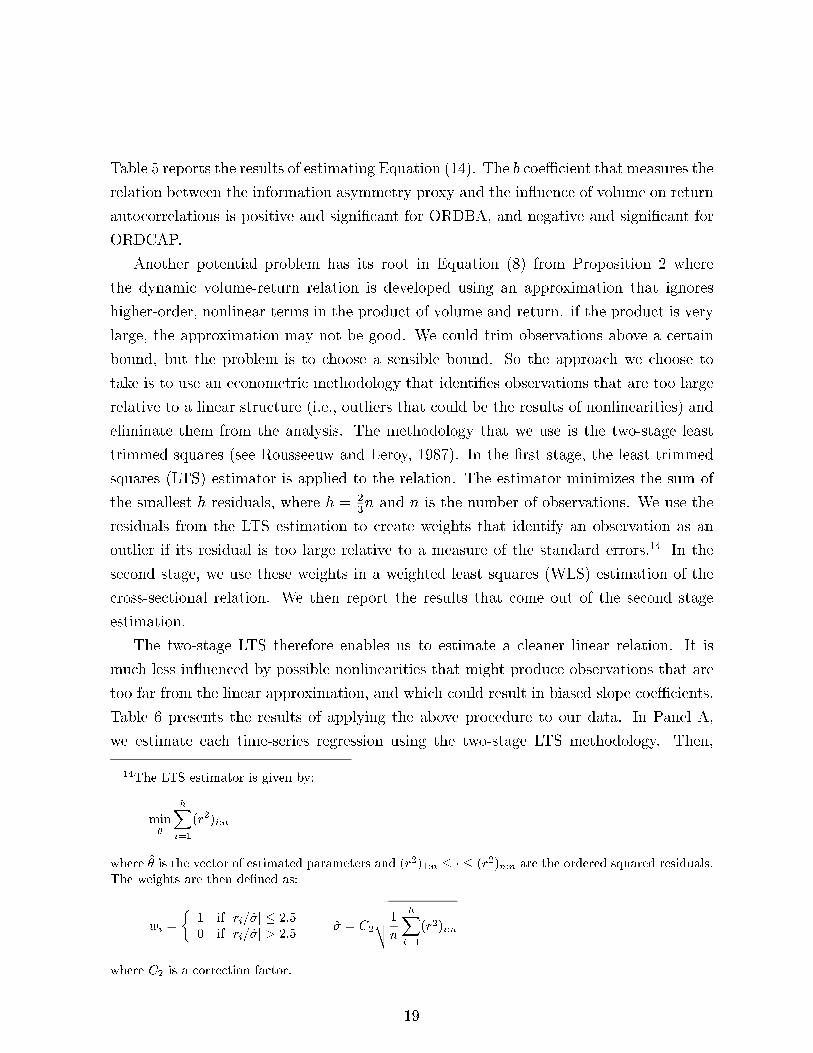
Table 5 reports the results of estimating Equation (14). The b coeÆcient that measures the

relation between the information asymmetry proxy and the in uence of volume on return

autocorrelations is positive and signi�cant for ORDBA, and negative and signi�cant for

ORDCAP.

Another potential problem has its root in Equation (8) from Proposition 2 where

the dynamic volume-return relation is developed using an approximation that ignores

higher-order, nonlinear terms in the product of volume and return. if the product is very

large, the approximation may not be good. We could trim observations above a certain

bound, but the problem is to choose a sensible bound. So the approach we choose to

take is to use an econometric methodology that identi�es observations that are too large

relative to a linear structure (i.e., outliers that could be the results of nonlinearities) and

eliminate them from the analysis. The methodology that we use is the two-stage least

trimmed squares (see Rousseeuw and Leroy, 1987). In the �rst stage, the least trimmed

squares (LTS) estimator is applied to the relation. The estimator minimizes the sum of

the smallest h residuals, where h = 23n and n is the number of observations. We use the

residuals from the LTS estimation to create weights that identify an observation as an

outlier if its residual is too large relative to a measure of the standard errors.14 In the

second stage, we use these weights in a weighted least squares (WLS) estimation of the

cross-sectional relation. We then report the results that come out of the second stage

estimation.

The two-stage LTS therefore enables us to estimate a cleaner linear relation. It is

much less in uenced by possible nonlinearities that might produce observations that are

too far from the linear approximation, and which could result in biased slope coeÆcients.

Table 6 presents the results of applying the above procedure to our data. In Panel A,

we estimate each time-series regression using the two-stage LTS methodology. Then,

14The LTS estimator is given by:

min�̂

hXi=1

(r2)i:n

where �̂ is the vector of estimated parameters and (r2)1:n � � � (r2)n:n are the ordered squared residuals.

The weights are then de�ned as:

wi =

�1 if jri=�̂j � 2:5

0 if jri=�̂j > 2:5�̂ = C2

vuut 1

n

hXi=1

(r2)i:n

where C2 is a correction factor.

19

we estimate Equation (12), the cross-sectional regression, by using OLS. The results are

similar to those reported in Tables 2 and 3: The coeÆcients of the information asymmetry

proxies are highly signi�cant and in the right direction. Hence, it does not seem as if very

large observations are adversely a�ecting the estimates of the parameters C2.

Because we do not know the functional form of the relation between information

asymmetry and the proxy we use, we can also apply the two-stage LTS approach to our

cross-sectional estimation. We use the C2 estimates that come out of the OLS time-series

estimation to allow for a cleaner comparison with the results in Tables 2 and 3. Panel B

of Table 6 presents the result of estimating the cross-sectional regression using two-stage

LTS. The results are similar to those of the OLS estimation.

Lastly, we repeat our cross-sectional analysis using the non-parametric Spearman cor-

relations. We wish to measure the association between the C2 coeÆcients and the in-

formation asymmetry proxies without imposing the OLS assumptions (e.g., normality of

the residuals). The Spearman correlation between C2 and ORDBA is 0.326 (asymptotic

standard error 0.02), and the correlation between C2 and ORDCAP is -0.26 (asymptotic

standard error 0.02). Hence, the Spearman correlations point to the same conclusions as

all our other econometric procedures.

We can ask several questions about the results presented so far. First, how do our

choices for the length of the time-series estimation period or the daily intervals for return

and volume a�ect our results? Second, can our results be attributed to the e�ect of bid-

ask bounce? Third, how sensitive are our results to the exact de�nition of volume that we

use? Fourth, can we relate our �ndings about information asymmetry to a variable that is

more directly associated with information production? Fifth, is �rm-speci�c information

asymmetry a driving force behind the dynamic volume-return relation or does the relation

disappear when we eliminate market-wide variations? The following sections address these

questions.

4.2 Alternative Lengths of Time Intervals

It is possible that the appropriate measurement period di�ers across stocks. For example,

for an infrequently traded stock, the period could be several days, so that more trades

are captured within the period. We might choose the appropriate measurement periods

to equate the quantities of noise trading (on average) across stocks. The measurement

interval is longer for stocks with little noise trading than it is for stocks with a lot of

noise trading. While we do not have a measure of noise trading, we can use the typical

20

turnover of a stock as a proxy for the normal level of trading. A typical trading intensity

measured by the stock's median turnover is less sensitive to informational or allocational

volume shocks.

Therefore, we calculate the median daily turnover for each stock over the sample

period (MedTurn), and assign all stocks into three groups according to their median

turnover. The average MedTurn for the three groups are 0.0634%, 0.1691%, and 0.384%,

respectively. we note that the average MedTurn of the High group is about twice that

of the Medium group and about �ve times that of the Low group. (The proportions

are similar when we use the cross-sectional median rather the average of each group.)

Therefore, given a daily interval for the most active stocks, we choose a two-day interval

as the most appropriate for the Medium group, and a �ve-day interval for the Low turnover

group. To calculate the return and turnover series for the Medium and Low groups, we

compound returns and sum the turnover for the days in the interval.

We then perform a separate time-series analysis for each stock. A stock in the High

MedTurn group that is listed for the entire sample period will have 1,516 observations

in the regressions, while a similar stock in the Medium (Low) MedTurn group will have

758 (303) observations. Taking the C2 coeÆcient from each individual stock's time-series

regression, we estimate the cross-sectional relation in Equation (12). We present the

cross-sectional results in Table 7, Panel A. The bid-ask spread coeÆcient is positive and

highly signi�cant, and the size coeÆcient is negative and highly signi�cant. Our results do

not appear to be driven by the choice of the daily interval for the time-series regressions.

Thus, whether we �x a time interval (a day in our experiment) or a given quantity of

noise trading (as the current test implies) does not a�ect our �ndings.

In Panel B of Table 7, we use ten instead of six years to estimate the time-series

regressions. This experiment allows us to check the sensitivity of our results to the length

of the estimation period. We estimate the volume-return interaction parameters (C2) in

this panel by using data from 1989 through 1998. The coeÆcients of the information

asymmetry proxies in the cross-sectional analysis have the right signs and are highly

statistically signi�cant.15

15While not reported in a table, we have also conducted the experiment with a sample of NYSE and

AMEX stocks using the period 1983-1992. The results are the same as those presented in the paper.

21

4.3 Information E�ects vs. Bid-Ask Bounce E�ects

Many studies show that short-horizon returns of individual stock exhibit negative auto-

correlation (e.g., French and Roll, 1986; Lo and MacKinlay, 1988; Conrad, Kaul, and

Nimalendran, 1991; Jegadeesh and Titman, 1995; Canina, Michaely, Thaler, and Wom-

ack, 1998). These autocorrelations are more pronounced in small stocks than in large

stocks. French and Roll (1986) and Jegadeesh and Titman (1995) show that the �rst

order autocorrelation of daily returns is negative for small stocks, increases with the size

of the �rm, and is positive for large �rms. Our sample shows the same results. The �rst-

order autocorrelation of daily returns is negative for stocks with large bid-ask spreads

(-0.088) and small stocks (-0.076). It is positive but very small for large stocks (0.003)

and stocks with small bid-ask spreads (0.01). These autocorrelations are similar in sign

and relative magnitude to the C1 coeÆcients from Tables 2 and 3.

Lo and MacKinlay (1988) suggest that these empirical �ndings are consistent with

security returns that re ect three in uences: a positively autocorrelated common com-

ponent, a white noise component, and a negative autocorrelation e�ect induced by mi-

crostructure phenomena such as bid-ask bounce. French and Roll (1986) suggest that the

positive autocorrelation arises when the market does not incorporate information as soon

as it is released. Jegadeesh and Titman (1995) attribute the negative autocorrelation to

inventory control by specialists.

Our model shows how volume should interact with the autocorrelation of returns.

For stocks with more information asymmetry, greater volume should make the �rst-order

autocorrelation more positive (hence, a positive C2) due to the partial adjustment of

prices to information. For stocks with less information asymmetry, greater volume should

make the �rst-order autocorrelation more negative (hence a negative C2) due to the return

reversal associated with liquidity shocks. However, for small stocks or stocks with large

bid-ask spreads, the prediction of our model and the bid-ask bounce e�ect both operate

in the same direction. We show that for stocks with large bid-ask spreads that exhibit

negative return autocorrelation, increased volume makes the autocorrelation less negative

(a positive C2). We claim that the positive C2 is the result of a high degree of information

asymmetry. However, we would expect a positive C2 if more volume decreases the bid-ask

bounce e�ect.

To examine this issue, we generate a return series that is free from bid-ask bounce.

Using the TAQ database, we identify the end-of-day quote for all days in our sample period

for all stocks (except Berkshire Hathaway Inc. that is excluded due to its abnormal price

22

range). We then construct a return series from the mid-quotes, and adjust for stock and

cash distributions using information from the CRSP database. We note that this return

series is less reliable than the CRSP series used in the main analysis. First, there are more

days without a valid end-of-day quote in the TAQ database than there are days without

a valid return in the CRSP database. Each day without an end-of-day quote results in

two days without valid mid-quote returns. Second, the intraday quote data in TAQ could

contain more errors than the heavily used CRSP return series.

The mid-quote return series eliminates most of the negative autocorrelation in the

returns of small stocks. For example, the �rst-order autocorrelation for the group of

small stocks (742 �rms) goes from -0.076 to -0.015, and that of the group of stocks

with large bid-ask spreads goes from -0.088 to -0.014. Our goal is to estimate the time-

series regressions using the mid-quote returns, and then examine the impact of these new

estimates on the cross-sectional relation that our model predicts (the relation between C2

and the information asymmetry proxies). We re-estimate Equation (10) with the mid-

quote return series for the �rms in our sample. An indication that the aforementioned

problems with respect to the mid-quote return series might have some e�ect is that the

time-series regressions using TAQ returns produce a few outliers of the C2 coeÆcient

while the time-series regressions using CRSP returns do not produce any outliers. Hence,

we estimate the cross-sectional relations using the two-stage LTS procedure described in

Section 4.1 to identify and eliminate the in uence of outliers. Table 8 presents the cross-

sectional regressions of ORDBA and ORDCAP on the interaction parameter C2. The

information asymmetry proxies have the appropriate signs and are statistically signi�cant.

We note, though, that the proxies explain less of the variation in the C2 coeÆcients than

they do in the cross-sectional regressions reported in Tables 2 and 3.

4.4 Alternative De�nitions of Volume

Since there is a slight di�erence between our de-trended volume measure and the theoret-

ical volume measure, Table 9 presents the results using alternative de�nitions of volume.

In Panel A, we de�ne volume as the daily share turnover of a stock, without taking

any transformation or detrending. We re-estimate the time-series relation in Equation

(10) with this alternative volume de�nition. The results of the cross-sectional regressions

show a statistically signi�cant relation, in the appropriate direction, between C2 and both

information asymmetry proxies.

In Panel B, we perform a more direct test of the relation in Equation (8) that comes

23

out of our theoretical model. In the theoretical model, it is the squared volume, rather

than a linear term, that a�ects the subsequent period's returns. We de�ne volume as

the logarithm of (1 + daily number of shares traded).16 Then we estimate the following

relation:

Rit+1 = C0i + C1i �Rit + C2i � V2itRit + errorit+1 (15)

The resulting cross-sectional analysis shows the same pattern as in Tables 2 and 3. In

fact, it appears that the relation is even stronger. Both information asymmetry proxies

explain over 16% of the cross-sectional variation in the parameter C2.

4.5 Analyst Following as a Proxy for Information Production

While the information asymmetry proxies we use in the main analysis have received much

attention in the literature, several recent papers discuss the relation between the number

of analysts who follow a stock and information asymmetry or adverse selection costs.

Early papers used the number of analysts as a direct proxy for informed trading, but

recent studies by Brennan and Subrahmanyam (1995), and Easley, O'Hara, and Paperman

(1998) �nd that �rms that are followed by a larger number of analysts have a lower degree

of information asymmetry or lower adverse selection costs.17 Thus, the number of analysts

appears to be negatively related to the degree of information asymmetry.

Using the number of analysts as a proxy for the degree of information asymmetry

has an intuitive appeal since it directly relates to information production in the market.

Nonetheless, this empirical proxy has its share of problems. First, there is still some doubt

about the direction and strength of the proxy's relation to the degree of information

asymmetry. Second, many stocks are not regularly followed by analysts. Third, the

number of analysts is heavily in uenced by membership in a particular industry. Fourth,

there is relatively little cross-sectional variation in the number of analysts who follow

stocks. Therefore, there are reasons to believe that the number of analysts will not

exhibit as strong a cross-sectional relation with C2 as will our two main proxies, bid-ask

spread and market capitalization.

To construct the analyst-following proxy, we look for the monthly number of analysts

who provide I/B/E/S with end-of-�scal-year earnings forecast for the current year. We

16To avoid taking the log of zero on days without trading, we add the small constant (1.00) to the daily

number of shares traded before making the logarithm transformation.

17See Easley, O'Hara, and Paperman (1998) for a discussion of the issue and additional references.

24

de�ne NumEsti to be the average monthly number of analysts over the sample period

(six years). ORDESTi is the ordinal scale of NumEsti (constructed like ORDBA and

ORDCAP), where two �rms that have the same number of analysts receive the same

rank. Out of the 2,226 �rms in our sample, 2,035 are followed by at least one analyst.

Not surprisingly, the majority of �rms without analyst coverage are in the Small size

group. Only 571 out of 742 �rms in the Small size group had forecast records in the

I/B/E/S database. The average number of analysts is 2.45 for those small �rms that are

being followed, compared with 16.51 for �rms in the Large size group.

Table 10 contains the results of the cross-sectional regression in Equation (12) using

either NumEst or ORDEST as the information asymmetry proxy. The coeÆcient of

NumEst is negative and statistically signi�cant and so is the coeÆcient of ORDEST,

though the relation is weaker than the cross-sectional results reported in Tables 2 and

3, where we use our two main proxies. Interpreting this result is straightforward. The

more analysts who cover a �rm, the better the production of information about the �rm's

prospects. Investors in a �rm with more information production have fewer opportunities

to engage in speculative trading, and therefore most trading in these �rms' securities

is motivated by hedging. Our results are consistent with the evidence in Brennan and

Subrahmanyam (1995) and Easley, O'Hara, and Paperman (1998), who �nd that the

number of analysts is negatively related to the degree of information asymmetry.

4.6 Firm-Speci�c Information Asymmetry

It is possible, and even likely, that both market-wide and �rm-speci�c factors drive the

trading and returns of individual stocks. In the model presented in Section 2, trading

is only generated by the �rm-speci�c hedging needs and private information. Thus, we

focus on the di�erent degree of �rm-speci�c private information as the main factor that

produces the cross-sectional variation in the dynamic volume-return relation. The model's

prediction on the relation between volume and return autocorrelation would therefore

most reasonably apply to the �rm-speci�c components of trading and returns.

We can test empirically whether the volume-return relation has a �rm-speci�c compo-

nent or if it disappears when we eliminate market-wide variations. To do so, we use market

models to decompose both the volume and return series. Each series is decomposed into a

systematic (market) component and a non-systematic (�rm-speci�c) component. To im-

plement the market models, we construct market return and volume series. The market's

return for a speci�c day is de�ned as the return on a value-weighted portfolio comprised

25

of all common stocks that traded on the NYSE or AMEX, and which have valid return

and volume information in the CRSP database for that day. We de�ne the market's

turnover in an analogous fashion as the value-weighted average of the turnover of the

individual stocks in the portfolio of all NYSE and AMEX common stocks. To maintain

compatibility, we detrend the log market turnover series, just as we do with the turnover

series of each individual stock. While sensible, this paper does not explicitly model this

particular volume decomposition. In a recent study, Lo and Wang (2000) present a formal

justi�cation for a market model of volume, which we use here.

We re-estimate Equation (10) by using residual returns and residual volume from the

respective market models. We then examine cross-sectional di�erences in the resulting C2

coeÆcients of the volume-return interaction terms. Table 11 presents the cross-sectional

regressions of the information asymmetry proxies on the C2 coeÆcients. The coeÆcient

of ORDBA is positive and statistically signi�cant, and the coeÆcient of ORDCAP is

negative and statistically signi�cant. These results suggest that �rm-speci�c information

asymmetry is a driving force behind the relation between volume and return autocorre-

lations.

5 Conclusions

We construct a simple model in which investors trade in the stock market for both hedging

and speculation motives. We use the model's insights to investigate the dynamic relation

between volume and returns. According to our model, returns generated by hedging-

motivated trades reverse themselves, while returns generated by speculation-motivated

trades tend to continue themselves. The relative signi�cance of these two types of trades

for an individual stock determines whether returns that are accompanied by trading vol-

ume exhibit negative or positive autocorrelation.

We test the model's predictions by using daily return and volume data for NYSE and

AMEX stocks. We look at how volume a�ects the �rst-order autocorrelation of daily

stock returns. To proxy for information asymmetry, we use bid-ask spreads (larger bid-

ask spreads imply a higher degree of information asymmetry) and market capitalization

(larger �rms are associated with less information asymmetry).

The empirical results support the predictions of the model on the nature of the dynamic

volume-return relation. Stocks that are associated with a high degree of informed trading

exhibit more return continuation on high-volume days, and stocks that are associated with

a low degree of informed trading show more return reversals on high-volume days. Our

26

results are robust to various econometric speci�cations, alternative de�nitions of volume,

and changes in the lengths of the measurement intervals and the estimation period. We

also show that the dynamic volume-return relation remains signi�cant after accounting

for possible bid-ask bounce e�ects.

We use analyst following as an additional proxy for the degree of information produc-

tion about a �rm. We �nd that in the portion of our sample for which we could �nd

data on analyst following, the dynamic volume-return relation shows the same pattern as

with the other information asymmetry proxies. We also investigate whether �rm-speci�c

information asymmetry is a driving force behind this relation. We use market models to

decompose returns and volume, and �nd that the relation holds even when we use only

�rm-speci�c (residual) returns and volume.

The empirical �ndings support the general notion that volume does tell us something

about future price movements. The analysis also suggests that the actual dynamic relation

between volume and returns depends on the underlying forces driving trading. Explicitly

modeling these driving forces allows us to use volume e�ectively in making an inference

about returns. In particular, by considering both allocational and informational trading,

our model gives rise to realistic predictions that seem to encompass the variety that

prevails in the market. It is this feature of the model that enables us to reconcile the

previous empirical �ndings of return reversals after high-volume days exhibited by large

�rms and indices, with the return continuation after high-volume days shown by average

�rms. The key to generating both results is our ability to use information asymmetry to

capture the cross-sectional variation in the dynamic volume-return relation of individual

stocks.

27

Appendix

Proof of Proposition 1. We consider the special case when Z(2)t = 0 8 t. Extending

the result to the general case is straightforward. We re-express the price as:

Pt = Ft + ~Pt

where ~Pt � a(Gt�bZt), b � b(1)=a and Zt � Z(1)t . We have

E(i)t [Rt+1] = E

(i)t [Dt+1]� Pt = E

(i)t [Gt]� ~Pt and �(i)

R

2 = �(i)D

2 + �2F+ �~P

2

where �(i)D

2 = E(i)t [G2

t ] and �2~P = a2(�2

G+ b2�2

Z). Note that E

(1)t [Gt] = Gt, E

(2)t [Gt] =

(Gt� bZt), �(1)DD = 0, and �

(2)D

2 = �2G, where = (�2

G+b2�2

Z)�1

�2G. Investors' stock

demands are:

X(1)t =

�Gt�

~Pt��DNZt

�=�(1)

R

2 and X(2)t =

h (Gt�bZt)� ~Pt

i=�(2)

R

2:

Market clearing requires that 0 = !X(1)t +(1�!)X

(2)t . Substituting in the investors' stock

demands, we have

0 = !(1� a)=�(1)R

2 + (1�!)( � a)=�(2)R

2

0 = !(�DN � ab)=�(1)R

2 + (1�!)( � a)b=�(2)R

2:

We can immediately solve for b: b = ��DN . Note that and �(i)DD (i = 1; 2) depend only

on b, not on a. We have the following equation for a:

0 = !�(2)R

2(1� a) + (1�!)�(1)R

2( � a):

Reorganizing terms, we have

0 = f(a) �ha2��2G+ b2�2

Z

�+��2F+ ! �2

G

�i(a� �a)� ! �2

G(1� �a)

where �a = 1� (1�!)(1� ) � 0. First, note that for a < �a, f(�a) < 0. Thus, f(a) = 0 has

no real roots less than �a. Second, note that f(�a) � 0 and f(a) ! 1 as a ! 1. Thus,

f(a) = 0 has a real root no less than �a. Third, f 0(a) > 0 for a > �a. We conclude that

f(a) = 0 has a unique root, which is non-negative. 2

Proof of Proposition 2. Suppose that x, y, z are jointly normally distributed with zero

means and a covariance matrix of � where

� =

0B@

�xx �xy �xz�xy �yy �yz�xz �yz �zz

1CA �

�11 �12

�0

12 �22

!

28

�11 = �xx, �12 = (�xy; �xz), and �22 = ((�yy; �yz); (�yz; �zz)). Then, we have

E[xjy; z] = �xyy + �xzz

where �xy =��12�

�122

�1and �xz =

��12�

�122

�2. Let f+ � exp

��

���1

22

�yzyjzj

�and

f�� exp

�+���1

22

�yzyjzj

�. Then

E[xjy; jzj] = �xyy +f+ � f

�

f+ + f�

�xzjzj = �xyy � �xzjzj tanh

����1

22

�yzjzjy

�

� �xyy � �xz

���1

22

�yzjzj2y:

For our purpose, let x = Rt+1, y = Rt and z = ~Pt�~Pt�1. Then, �xx = �yy = (1� a)2�2

G+

a2�2DN�2Z+ �2

R, �zz = 2�2

~P , �xy = a�2G� �2

~P , �xz = a�2G� �2

~P , and �yz = 2�2~P � a�2

G, where

�2R= �2

F+ �2

~P . Then, we have

E

�Rt+1

����Rt; j ~Pt �~Pt�1j

�= �1Rt � �2j ~Pt �

~Pt�1j tanh��j ~Pt �

~Pt�1jRt

��

��1 � �02j

~Pt �~Pt�1j

2�Rt

where

�1 = �xy = �

a�2G(�2

~P � a�2G)

2�2D�2~P � a2�4

G

�2 =(�2

D� a�2

G)(�2

~P � a�2G)

2�2D�2~P � a2�4

G

� =2�2

~P � a�2G

2�2D�2~P � a2�4

G

�1 = �1

�02 = �2�

where �2D= �2

F+ �2

G. Since �2

~P = a(�2G+ b2�2

Z)(a� ) and a � �a � , we have �2 � 0 and

� � 0. Further note that j ~Pt�~Pt�1j =

q(2=�)�~P

~Vt. Letting �2 = 2�2~P�

0

2=�, we obtain (8).

2

Proof of Proposition 3. For �2G= 0, a = !, �02 = 1=(2�2

D), and

�2 = �20 =�2~P

��2D

�

!2

�

�2DN�2Z

�2D

For �2Gsmall and holding �2

D, �2

~P constant, we have

�2 �1

�

�2D

�2~P

"1� a

�2G

�2D

+3

2

�2G

�2~P

!#+ o(�2

G):

Realizing that a = ! + o(�2G), we obtain Equation (9). 2

29

References

Ajinkya B.B., and P.C. Jain, 1989, The Behavior of Daily Stock Market Trad-

ing Volume, Journal of Accounting and Economics 11, 331-359.

Antoniewicz, R.L., 1993, Relative Volume and Subsequent Stock Price Move-

ments, working paper, Board of Governors of the Federal Reserve System.

Bhattacharya, U. and M. Spiegel, 1991, Insiders, Outsiders, and Market Break-

downs, Review of Financial Studies 4, 255-282.

Blume, L., D. Easley, and M. O'Hara, 1994, Market Statistics and Technical

Analysis: The Role of Volume, Journal of Finance 49, 153-181.

Brennan, M. and A. Subrahmanyam, 1995, Investment Analysis and Price

Formation in Securities Markets, Journal of Financial Economics 38, 361-

381.

Breusch, T.S., 1978, Testing for Autocorrelation in Dynamic Linear Models,

Australian Economic Papers 17, 334-355.

Brown, D.P., and R.H. Jennings, 1989, On Technical Analysis, Review of

Financial Studies 2, 527-551.

Campbell, J.Y., S.J. Grossman, and J. Wang, 1993, Trading Volume and

Serial Correlation in Stock Returns, Quarterly Journal of Economics 108,

905-939.

Canina, L., R. Michaely, R. Thaler, and K. Womack, 1998, Caveat Com-

pounder: A Warning about Using the Daily CRSP Equal-Weighted Index

to Compute Long-Run Excess Returns, Journal of Finance 53, 403-416.

Conrad, J., A. Hameed, and Niden C.M., 1992, Volume and Autocovariances

in Short-Horizon Individual Security Returns, Journal of Finance 49, 1305-

1329.

Conrad, J., G. Kaul, and M. Nimalendran, 1991, Components of Short-Horizon

Individual Security Returns, Journal of Financial Economics 29, 365-384.

Cready, W.M., and Ramanan R., 1991, The Power of Tests Employing Log-

Transformed Volume in Detecting Abnormal Trading, Journal of Account-

ing and Economics 14, 203-214.

30

Du�ee, G., 1992, Trading volume and Return Reversals, Finance and Eco-

nomics Discussion Paper Series No. 192, Board of Governors of the Federal

Reserve System.

Easley, D., and M. O'Hara, 1987, Price, Trade Size, and Information In Secu-

rities Markets, Journal of Financial Economics 18, 69-90.

Easley, D., M. O'Hara, and J. Paperman, 1998, Are Financial Analysts In-

formed Traders? Journal of Financial Markets 1, 175-201.

French, K.R., and R. Roll, 1986, Stock Return Variances: The Arrival of

Information and the Reaction of Traders, Journal of Financial Economics

17, 5-26.

Gallant, R., P. Rossi, and Tauchen, G., 1992, Stock Prices and Volume, Review

of Financial Studies 5, 199-242.

Glosten, L. and P. Milgrom, 1985, Bid, Ask and Transaction Prices in a

Market-Maker Market with Heterogeneously Informed Traders, Journal

of Financial Economics 14, 71-100.

Godfrey, L.G., 1978a, Testing Against General Autoregressive and Moving

Average Error Models when the Regressors Include Lagged Dependent

Variables, Econometrica 46, 1293-1302.

Godfrey, L.G., 1978b, Testing Against Higher Order Serial Correlation in Re-

gression Equations when the Regressors Include Lagged Dependent Vari-

ables, Econometrica 46, 1303-1310.

Grundy, B., and M. McNichols, 1989, Trade and Revelation of Information

through Prices and Direct Disclosure, Review of Financial Studies 2, 495-

526.

Hasbrouck, J., 1988, Trades, Quotes, Inventories, and Information, Journal of

Financial Economics 22, 229-252.

Hasbrouck, J., 1991, Measuring the Information Content of Stock Trades,

Journal of Finance 46, 179-207.

He, H., and J. Wang, 1995, Di�erential Information and Dynamic Behavior of

Trading Volume, Review of Financial Studies 8, 919-972.

Jegadeesh, N., and S. Titman, 1995, Short-Horizon Return Reversals and the

Bid-Ask Spread Journal of Financial Intermediation 4, 116-132.

31

Johnston, J., 1985, Econometric Methods 3rd Edition, McGraw-Hill Book

Company.

Jorion, P., 1990, The Exchange-Rate Exposure of U.S. Multinationals, Journal

of Business 63, 331-345.

Kyle, Albert S.,1985, Continuous Auctions and Insider Trading, Econometrica

53, 1315-1335.

LeBaron, B., 1992, Persistence of the Dow Jones Index on Rising Volume,

working paper, University of Wisconsin.

Lee, C.M.C., B. Mucklow, and M.J. Ready, 1993, Spreads, Depths, and the

Impact of Earnings Information: an Intraday Analysis, Review of Financial

Studies 6, 345-374.

Lee, C.M.C. and B. Swaminathan, 2000, Price Momentum and Trading Vol-

ume, forthcoming, Journal of Finance.

Lo, A.W., and A.C. MacKinlay, 1988, Stock Market Prices Do Not Follow

Random Walks: Evidence from a Simple Speci�cation Test, Review of

Financial Studies 1, 41-66.

Lo, A.W., and A.C. MacKinlay, 1990, An Econometric Analysis of Nonsyn-

chronous Trading, Journal of Econometrics 45, 181-211.

Lo, A. and J. Wang, 2000, Trading Volume: De�nitions, Data Analysis, and

Implications of Portfolio Theory, Review of Financial Studies 13, 257-300.

Madhavan, A., M. Richardson, and M. Roomans, 1997, Why Do Security

Prices Change? A Transaction-Level Analysis of NYSE Stocks, Review of

Financial Studies 10, 1035-1064.

Morse, D., 1980, Asymmetric Information in Securities Markets and Trading

Volume, Journal of Financial and Quantitative Analysis 15, 1129-1148.

Richardson G., S.E. Sefcik, and R. Thompson, 1986, A Test of Dividend Irrel-

evance Using Volume Reactions to a Change in Dividend Policy, Journal

of Financial Economics 17, 313-333.

Rousseeuw, P.J, and A.M. Leroy, 1987, Robust Regression and Outlier Detec-

tion, John Wiley & Sons.

32

Stickel, S.E. and R.E. Verrecchia, 1994, Evidence that Volume Sustains Price

Changes, Financial Analyst Journal (November-December), 57-67.

Wang, J., 1994, A Model of Competitive Stock Trading Volume, Journal of

Political Economy 102, 127-168.

33

34

Table 1 Summary Statistics

The sample contains 2,226 stocks. Included in the sample are all common stocks with information in the CRSP database that traded on the NYSE or AMEX between 1993 and 1998 and that had at least 1,000 days with trading. Panel A presents descriptive statistics by size groups. For each firm, AvgCapi is the average daily market capitalization (number of shares outstanding multiplied by the daily closing price). AvgTrd i is the average number of shares traded daily. AvgTurn i is the average daily turnover (number of shares traded divided by the number of shares outstanding), and AvgPrc i is the average price of a firm’s stock over the sample period. BAsprd i is the average daily opening percentage spread (opening bid-ask spread divided by the opening midquote) over the sample period from the TAQ database. Panel B presents descriptive statistics for the volume series used in the time-series regressions. We define the daily volume series of a stock as the detrended, log-transformed daily turnover series. We report the averages for the entire sample and for three size groups of the mean, standard deviation, and selected autocorrelation coefficients of the volume series of the individual stocks. Panel A: Characteristics of the Entire Sample and Three Size-Based Subsamples

AvgCap (in million $)

AvgTrd (in 100s)

AvgTurn (in %)

AvgPrc (in $)

BAsprd (in %)

Entire Sample Mean 2,587.55 1,997 0.321 25.59 2.19 Median 473.52 672 0.258 22.40 1.38 Std. Dev 8,019.00 3,844 0.255 20.49 2.33 Minimum 3.61 2 0.007 0.39 0.25 Maximum 147,817.21 52,735 2.837 330.45 19.51 Observations 2226 2226 2226 2225 2225Size Group: Mean 85.97 288 0.270 10.84 4.11Small Median 75.96 164 0.212 8.90 3.12 Std. Dev 58.18 408 0.213 7.79 2.99 Observations 742 742 742 742 741Size Group: Mean 525.98 918 0.338 23.93 1.62Medium Median 473.52 601 0.273 22.91 1.35 Std. Dev 237.23 994 0.263 11.24 1.13 Observations 742 742 742 742 742Size Group: Mean 7,150.69 4,786 0.355 42.01 0.84Large Median 3,111.11 2,863 0.291 37.20 0.75 Std. Dev 12,714.35 5,597 0.277 24.17 0.48 Observations 742 742 742 741 742

Panel B: Descriptive Statistics of the Volume (Detrended Log Turnover) Series

Mean Standard Deviation

First Autocorrelation

Fifth Autocorrelation

Tenth Autocorrelation

# of stocks

Entire Sample 0.028 1.068 0.370 0.193 0.143 2226Size group: Low 0.013 1.537 0.313 0.182 0.138 742Size group: Medium 0.038 1.000 0.366 0.196 0.148 742Size group: High 0.034 0.668 0.430 0.200 0.144 742

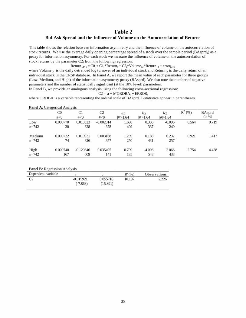
35

Table 2 Bid-Ask Spread and the Influence of Volume on the Autocorrelation of Returns

This table shows the relation between information asymmetry and the influence of volume on the autocorrelation of stock returns. We use the average daily opening percentage spread of a stock over the sample period (BAsprd i) as a proxy for information asymmetry. For each stock we measure the influence of volume on the autocorrelation of stock returns by the parameter C2i from the following regression:

Return i,t+1 = C0i + C1i*Return t + C2i*Volumei,t*Return i,t + errori,t+1 where Volume i,t is the daily detrended log turnover of an individual stock and Return i,t is the daily return of an individual stock in the CRSP database. In Panel A, we report the mean value of each parameter for three groups (Low, Medium, and High) of the information asymmetry proxy (BAsprd). We also note the number of negative parameters and the number of statistically significant (at the 10% level) parameters. In Panel B, we provide an analogous analysis using the following cross-sectional regression:

C2i = a + b*ORDBA i + ERRORi where ORDBA is a variable representing the ordinal scale of BAsprd. T-statistics appear in parentheses. Panel A: Categorical Analysis C0 C1 C2 tC0 tC1 tC2 R2 (%) BAsprd #<0 #<0 #<0 |#|>1.64 |#|>1.64 |#|>1.64 (in %) Low 0.000770 0.013323 -0.002814 1.698 0.336 -0.096 0.564 0.719 n=742 30 328 378 409 337 240 Medium 0.000722 0.010931 0.003168 1.239 0.188 0.232 0.921 1.417 n=742 74 326 357 250 431 257 High 0.000740 -0.120346 0.035495 0.709 -4.003 2.066 2.754 4.428 n=742 167 609 141 135 548 438 Panel B: Regression Analysis Dependent variable a b R2(%) Observations C2 -0.015921

(-7.863) 0.055716 (15.891)

10.197 2,226

36

Table 3 Market Capitalization and the Influence of Volume on the Autocorrelation of Returns

This table shows the relation between information asymmetry and the influence of volume on the autocorrelation of stock returns. We use the average market capitalization of a firm over the sample period (AvgCapi) as a proxy for information asymmetry. For each stock we measure the influence of volume on the autocorrelation of stock returns by the parameter C2i from the following regression:

Return i,t+1 = C0i + C1i*Return t + C2i*Volumei,t*Return i,t + errori,t+1 where Volume i,t is the daily detrended log turnover of an individual stock and Return i,t is the daily return of an individual stock in the CRSP database. In Panel A, we report the mean value of each parameter for three groups (Low, Medium, and High) of the information asymmetry proxy (AvgCap). We also note the number of negative parameters and the number of statistically significant (at the 10% level) parameters. In Panel B, we provide an analogous analysis using the following cross-sectional regression:

C2i = a + b*ORDCAPi + ERRORi where ORDCAP is a variable representing the ordinal scale of AvgCap. T-statistics appear in parentheses. Panel A: Categorical Analysis C0 C1 C2 tC0 tC1 tC2 R2 (%) AvgCap #<0 #<0 #<0 |#|>1.64 |#|>1.64 |#|>1.64 (in million $) Low 0.000784 -0.104234 0.030277 0.843 -3.538 1.848 2.729 85.97 n=742 139 557 167 157 550 429 Medium 0.000672 0.005492 0.004852 1.178 0.028 0.289 0.996 525.98 n=742 95 348 355 258 433 284 High 0.000776 0.002650 0.000719 1.625 0.032 0.065 0.514 7150.69 n=742 37 358 354 379 333 222 Panel B: Regression Analysis Dependent variable a b R2(%) Observations C2 0.034081

(16.488) -0.044242 (-12.362)

6.430 2,226

37

Table 4 Alternative Econometric Specifications: Autoregressive Structure

For each stock, we measure the influence of volume on the autocorrelation of stock returns by the parameter C2i from the following regression:

Return i,t+1 = C0i + C1i*Return t + C2i*Volumei,t*Return i,t + errori,t+1

where Volumei,t is the daily detrended log turnover of an individual stock and Return i,t is the daily return of an individual stock in the CRSP database. For each stock, we test for white noise against the alternative of an autoregressive error structure of orders one through five using the Breusch-Godfrey test. We use a 5% significance level to reject the white noise hypothesis. In Panel A, we identify the most appropriate autoregressive structure using Algorithm A as follows: If the test is significant for any order p<5 but not for higher orders, we test again with the null of AR(p) against an autoregressive structure of orders higher than p, but only up to order five. After identifying the appropriate order, we estimate the above relation using maximum likelihood with the suitable autoregressive structure. In Panel B, we identify the autoregressive structure using Algorithm B, which uses only the white noise test against an AR structure for each individual stock. Both panels report the results of the cross-sectional regressions:

C2i = a + b*ORDBA i + ERRORi C2i = a + b*ORDCAPi + ERRORi

where ORDBA and ORDCAP are variables representing the ordinal scales of BAsprd and AvgCap, respectively. T-statistics appear in parentheses.

Panel A: Autoregressive Structure Identified Using Algorithm A C2i = a + b*ORDBA i + ERRORi

a b R2(%) Observations -0.015298

(-7.048) 0.060185 (16.014)

10.339 2,226

C2i = a + b*ORDCAPi + ERRORi

a b R2(%) Observations 0.038386 (17.303)

-0.047135 (-12.271)

6.341 2,226

Panel B: Autoregressive Structure Identified Using Algorithm B C2i = a + b*ORDBA i + ERRORi

a B R2(%) Observations -0.015485

(-7.154) 0.060403 (16.118)

10.459 2,226

C2i = a + b*ORDCAPi + ERRORi

a b R2(%) Observations 0.038443 (17.376)

-0.047403 (-12.374)

6.442 2,226

38

Table 5 Alternative Econometric Specifications: Sensitivity to Common Factor

For each stock, we measure the influence of volume on the autocorrelation of stock returns by the parameter D2i from the following time-series regression:

Return i,t+1 = D0i + D1i*Return t + D2i*Volumei,t*Return i,t + D3*MktRett+1 + errori,t+1

MktRett+1 is the return on a value-weighted portfolio comprised of all common stocks that traded on the NYSE or AMEX that have valid return and volume information in the CRSP database for that day. The incorporation of MktRett+1 in the time-series regressions is intended to reduce potential correlation of the errors across stocks that arises from sensitivity to common factors. We report the results of the cross-sectional regressions:

D2i = a + b*ORDBA i + ERRORi D2i = a + b*ORDCAPi + ERRORi

where ORDBA and ORDCAP are variables representing the ordinal scales of BAsprd and AvgCap, respectively. T-statistics appear in parentheses. D2i = a + b*ORDBA i + ERRORi

a b R2(%) Observations -0.005528

(-2.795) 0.043256 (12.631)

6.693 2,226

D2i = a + b*ORDCAPi + ERRORi

a b R2(%) Observations 0.031677 (15.745)

-0.031121 (-8.934)

3.465 2,226

39

Table 6 Alternative Econometric Specifications: Least Trimmed Squares

For each stock, we measure the influence of volume on the autocorrelation of stock returns by the parameter C2i from the following regression:

Return i,t+1 = C0i + C1i*Return t + C2i*Volumei,t*Return i,t + errori,t+1

where Volume i,t is the daily detrended log turnover of an individual stock and Return i,t is the daily return of an individual stock in the CRSP database. We estimate this relation in two stages. In the first stage, we use a least trimmed squares (LTS) estimator to identify outliers (by minimizing the sum of the h smallest squared residuals, where h=2/3 of the observations for each stock). In the second stage, we use a weighted least squares (WLS) estimation in which we make the weights on the outliers identified in the first stage equal to zero. The C2i parameters for the cross-sectional estimation are taken from the WLS estimation. In Panel A, we report the results of the OLS cross-sectional regressions:

C2i = a + b*ORDBA i + ERRORi C2i = a + b*ORDCAPi + ERRORi

where ORDBA and ORDCAP are variables representing the ordinal scales of BAsprd and AvgCap, respectively. In Panel B, we apply the two-stage LTS estimation to the cross-sectional, rather than the time-series, regressions. We take the C2i coefficients from the OLS time series regressions that were presented in Tables 2 and 3, but we use LTS to estimate the relations with the information asymmetry proxies. We present the results of the second-stage WLS estimation. T-statistics appear in parentheses.

Panel A: Two-Stage Least Trimmed Squares Applied to Time-Series Regressions C2i = a + b*ORDBA i + ERRORi

a b R2(%) Observations -0.011487

(-5.483) 0.049199 (13.562)

7.638 2,226

C2i = a + b*ORDCAPi + ERRORi

a b R2(%) Observations 0.032918 (15.487)

-0.039572 (-10.752)

4.942 2,226

Panel B: Two-Stage Least Trimmed Squares Applied to Cross-Sectional Regressions C2i = a + b*ORDBA i + ERRORi

a B R2(%) Observations -0.019349

(-10.40) 0.060732

(19.00) 14.328 2,226

C2i = a + b*ORDCAPi + ERRORi

a b R2(%) Observations 0.034651

(18.57) -0.046424

(-14.25) 8.586 2,226

40

Table 7 Alternative Lengths of Time Intervals

Panel A replaces the daily interval for measuring return and volume with an alternative interval that allows for roughly the same level of noise trading across stocks. We use the median daily turnover (MedTurn) of a stock as a measure of the normal level of trading. We group all stocks into three categories (High, Medium and Low) according to their MedTurn. We use a daily interval for stocks in the High group, a two-day interval for stocks in the Medium group, and a five-day interval for stocks in the Low group (so that the average turnover across groups is equal). We calculate the return and turnover series for a stock in the medium and low groups by compounding daily returns and linearly adding turnover for the days in each interval. For each stock, we measure the influence of volume on the autocorrelation of stock returns by the parameter C2i from the following regression:

Return i,t+1 = C0i + C1i*Return t + C2i*Volumei,t*Return i,t + errori,t+1

where Volume i,t is the detrended log turnover of an individual stock and Return i,t is the return of an individual stock. We report the results of the OLS cross-sectional regressions:

C2i = a + b*ORDBA i + ERRORi

C2i = a + b*ORDCAPi + ERRORi where ORDBA and ORDCAP are variables representing the ordinal scales of BAsprd and AvgCap, respectively. In Panel B, we test the robustness of our results to a longer estimation period. We estimate the time series regressions for the stocks in our sample using 10 years of data (1989–1998). We present the results of the cross-sectional regressions using the same information asymmetry proxies as in Panel A. T-statistics appear in parentheses.

Panel A: Using an Alternative to the Daily Interval for Measuring Return and Volume C2i = a + b*ORDBA i + ERRORi

a B R2(%) Observations -0.015534

(-6.286) 0.038606

(9.023) 3.531 2,226

C2i = a + b*ORDCAPi + ERRORi

a b R2(%) Observations 0.016285

(6.521) -0.025003

(-5.782) 1.481 2,226

Panel B: Using Ten Years of Data (1989-1998) C2i = a + b*ORDBA i + ERRORi

a B R2(%) Observations -0.014592

(-8.118) 0.057887 (18.599)

13.461 2,226

C2i = a + b*ORDCAPi + ERRORi

a b R2(%) Observations 0.037995 (20.609)

-0.047240 (-14.799)

8.965 2,226

41

Table 8 Eliminating the Bid-Ask Bounce Effect

The influence of volume on the autocorrelation of stock returns is measured by the parameter C2i from the following time-series regression:

Return i,t+1 = C0i + C1i*Return i,t + C2i*Volumei,t*Return i,t + errori,t+1

To eliminate the effects of bid-ask bounce, we calculate Return i, from end-of-day mid-quotes. We report the results of the cross-sectional regressions:

C2i = a + b*ORDBA i + ERRORi

C2i = a + b*ORDCAPi + ERRORi where ORDBA and ORDCAP are variables representing the ordinal scales of BAsprd and AvgCap, respectively. To eliminate the effects of outliers, the cross-sectional regressions are estimated using the two-stage least trimmed squares procedure described in Section 4.1. C2i = a + b*ORDBA i + ERRORi

a b R2(%) Observations -0.020033

(-8.87) 0.028729

(7.45) 2.674 2,225

C2i = a + b*ORDCAPi + ERRORi

a b R2(%) Observations 0.006676

(3.01) -0.025449

(-6.52) 2.050 2,225

42

Table 9 Alternative Definitions of Volume

In Panel A, the influence of volume on the autocorrelation of stock returns is measured by the parameter C2i from the following time-series regression:

Return i,t+1 = C0i + C1i*Return t + C2i*Volumei,t*Return i,t + errori,t+1

where turnover (the daily number of shares traded divided by the number of shares outstanding) serves as the alternative definition of volume. In Panel B, the influence of volume on the autocorrelation of stock returns is measured by the parameter C2i from the following time-series regression:

Return i,t+1 = C0i +C1i* Return t + C2i* (Volumei,t)2 *Return i,t + errori,t+1

where log(1+daily number of shares traded) serves as the alternative definition of volume. Using the results of the time-series regressions, both panels report the results of the cross-sectional regressions:

C2i = a + b*ORDBA i + ERRORi C2i = a + b*ORDCAPi + ERRORi

where ORDBA and ORDCAP are variables representing the ordinal scales of BAsprd and AvgCap, respectively. T-statistics appear in parentheses. Panel A: Volume Is Measured as Turnover C2i = a + b*ORDBA i + ERRORi

a b R2(%) Observations -3.322436

(-3.869) 10.685070

(7.186) 2.269 2,226

C2i = a + b*ORDCAPi + ERRORi

a b R2(%) Observations 6.408573

(7.434) -8.768206

(-5.875) 1.528 2,226

Panel B: Volume Is Measured as log(1+Shares Traded) C2i = a + b*ORDBA i + ERRORi

a B R2(%) Observations -0.001029 (-11.917)

0.003526 (23.579)

19.999 2,226

C2i = a + b*ORDCAPi + ERRORi

a b R2(%) Observations 0.002335 (26.454)

-0.003199 (-20.934)

16.461 2,226

43

Table 10 Analyst Following as an Information Asymmetry Proxy

The influence of volume on the autocorrelation of stock returns is measured by the parameter C2i from the following time-series regression:

Return i,t+1 = C0i + C1i*Return t + C2i*Volumei,t*Return i,t + errori,t+1

To construct the proxy for analyst following, we look for the monthly number of analysts who provide I/B/E/S with an end-of-fiscal-year earnings forecast for the current year. NUMESTi is the average monthly number of analysts over the sample period (six years). We use this variable as a proxy for information asymmetry (the more analysts, the less information asymmetry). We use a reduced sample of 2035 firms for which we found information concerning analyst following in the I/B/E/S database. We report the results of the cross-sectional regressions:

C2i = a + b*NUMESTi + ERRORi

C2i = a + b*ORDESTi + ERRORi ORDESTi is a variable representing the ordinal scale of NUMESTi, where two firms that have the same number of analysts receive the same rank. T-statistics appear in parentheses. C2i = a + b*NUMESTi + ERRORi

a b R2(%) Observations 0.016435

(9.789) -0.000760

(-5.362) 1.395 2,035

C2i = a + b*ORDESTi + ERRORi

a b R2(%) Observations 0.022239 (10.970)

-0.026790 (-7.383)

2.611 2,035

44

Table 11 Firm-Specific Information Asymmetry and return-volume relation

This table contains an empirical test of the hypothesis that firm-specific information asymmetry is a driving force behind the dynamic relation between returns and volume. For each stock, we measure the influence of volume on the autocorrelation of stock returns by the parameter C2i from the following regression:

ResReturn i,t+1 = C0i + C1i*ResReturn i,t + C2i*ResVolume i,t*ResReturn i,t + errori,t+1 ResReturn i,t is the daily abnormal return of an individual stock. We define abnormal return as the residual of a market model in which the market return is constructed using a value-weighted portfolio comprised of all common stocks that traded on the NYSE or AMEX with valid return and volume information in the CRSP database for that day. ResVolume i,t is the residual volume of an individual stock. It is defined in a fashion analogous to abnormal return as the residual of a market model in which market volume is the daily detrended log turnover of the value-weighted portfolio. The table presents the results of the cross-sectional regressions:

C2i = a + b*ORDBA i + ERRORi C2i = a + b*ORDCAPi + ERRORi

where ORDBA and ORDCAP are variables representing the ordinal scales of BAsprd and AvgCap. T-statistics appear in parentheses. C2i = a + b*ORDBA i + ERRORi

a b R2(%) Observations 0.000740

(0.374) 0.038645 (11.277)

5.409 2,226

C2i = a + b*ORDCAPi + ERRORi

a b R2(%) Observations 0.033270 (16.559)

-0.026386 (-7.585)

2.522 2,226