dynamic modeling, trajectory generation and tracking for
TRANSCRIPT

Brigham Young University Brigham Young University
BYU ScholarsArchive BYU ScholarsArchive
Theses and Dissertations
2012-12-03
Dynamic Modeling, Trajectory Generation and Tracking for Towed Dynamic Modeling, Trajectory Generation and Tracking for Towed
Cable Systems Cable Systems
Liang Sun Brigham Young University - Provo
Follow this and additional works at: https://scholarsarchive.byu.edu/etd
Part of the Electrical and Computer Engineering Commons
BYU ScholarsArchive Citation BYU ScholarsArchive Citation Sun, Liang, "Dynamic Modeling, Trajectory Generation and Tracking for Towed Cable Systems" (2012). Theses and Dissertations. 3532. https://scholarsarchive.byu.edu/etd/3532
This Dissertation is brought to you for free and open access by BYU ScholarsArchive. It has been accepted for inclusion in Theses and Dissertations by an authorized administrator of BYU ScholarsArchive. For more information, please contact [email protected], [email protected].

Dynamic Modeling, Trajectory Generation and Tracking for Towed Cable Systems
Liang Sun
A dissertation submitted to the faculty ofBrigham Young University
in partial fulfillment of the requirements for the degree of
Doctor of Philosophy
Randal W. Beard, ChairJohn D. Hedengren
Tim W. McLainMark B. Colton
Wynn C. StirlingDah-Lye Lee
Department of Electrical and Computer Engineering
Brigham Young University
December 2012
Copyright c© 2012 Liang Sun
All Rights Reserved

ABSTRACT
Dynamic Modeling, Trajectory Generation and Tracking for Towed Cable Systems
Liang SunDepartment of Electrical and Computer Engineering
Doctor of Philosophy
In this dissertation, we focus on the strategy that places and stabilizes the path of anaerial drogue, which is towed by a mothership aircraft using a long flexible cable, onto a hor-izontally flat orbit by maneuvering the mothership in the presence of wind. To achieve thisgoal, several studies for towed cable systems are conducted, which include the dynamic mod-eling for the cable, trajectory generation strategies for the mothership, trajectory-trackingcontrol law design, and simulation and flight test implementations.
First, a discretized approximation method based on finite element and lumped mass isemployed to establish the mathematical model for the towed cable system in the simulation.Two approaches, Gauss’s Principle and Newton’s second law, are utilized to derive theequations of motion for inelastic and elastic cables, respectively. The preliminary studies forseveral key parameters of the system are conducted to learn their sensitivities to the systemmotion in the steady state. Flight test results are used to validate the mathematical modelas well as to determine an appropriate number of cable links.
Furthermore, differential flatness and model predictive control based methods areused to produce a mothership trajectory that leads the drogue onto a desired orbit. Differentdesired drogue orbits are utilized to generate required mothership trajectories in differentwind conditions. The trajectory generation for a transitional flight in which the system fliesfrom a straight and level flight into a circular orbit is also presented. The numerical resultsare presented to illustrate the required mothership orbits and its maneuverability in differentwind conditions. A waypoint following based strategy for mothership to track its desiredtrajectory in flight test is developed. The flight test results are also presented to illustratethe effectiveness of the trajectory generation methods.
In addition, a nonlinear time-varying feedback control law is developed to regulate themothership to follow the desired trajectory in the presence of wind. Cable tensions and winddisturbance are taken into account in the design model and Lyapunov based backsteppingtechnique is employed to develop the controller. The mothership tracking error is provedto be capable of exponentially converging to an ultimate bound, which is a function of theupper limit of the unknown component of the wind. The simulation results are presented tovalidate the controller.
Finally, a trajectory-tracking strategy for unmanned aerial vehicles is developed wherethe autopilot is involved in the feedback controller design. The trajectory-tracking controlleris derived based on a generalized design model using Lyapunov based backstepping. The aug-mentations of the design model and trajectory-tracking controller are conducted to involve

the autopilot in the closed-loop system. Lyapunov stability theory is used to guarantee theaugmented controller is capable of driving the vehicle to exponentially converge to and followthe desired trajectory with the other states remaining bounded. Numerical and Software-In-the-Loop simulation results are presented to validate the augmented controller. Thismethod presents a framework of implementing the developed trajectory-tracking controllersfor unmanned aerial vehicles without any modification to the autopilot.
Keywords: towed cable system, trajectory generation, trajectory tracking, model predictivecontrol, differential flatness, autopilot in the loop, aerial recovery

ACKNOWLEDGMENTS
I would like to express my deepest gratitude to my advisor Professor Randal W.
Beard for his guidance, support, enthusiasm and patience in all aspects of this research.
I would also like to express special thanks to Professor John D. Hedengren for his advice
and instruction of not only my research but my personal life. I highly appreciate that
Professor Tim W. McLain provided the TA opportunity in the final phase of my PhD study.
Also, Professor Mark B. Colton, Professor D. J. Lee and Professor Wynn C. Stirling are
particularly recognized for their support as my PhD committee.
I am extremely grateful for being a member of Aerial Recovery team and thankful
to team members Joseph Nichols, Neil Johnson, Jeff Ferrin, Mark Owen, Daniel Carlson,
Jesse Williams, Dallin Briggs, Steve Carlson and Nathan Ander. Without their help and
support, it would be impossible to successfully conduct flight tests and demo at Dugway,
Elberta and Mosida. I have also greatly benefitted from discussions with present and former
colleagues at MAGICC lab, Rajnikant Sharma, Huili Yu, Travis Millet, Everett Bryan,
Laith Sahawneh, John MacDonald, Peter Niedfeldt, Jeff Saunders, Nathan Edwards, Robert
Klaus, Robert Leishman, Brandon Cannon, Brandon Carroll, Jacob Bishop, David Casbeer,
Matthew Argyle, Jason Beach and Eric Quist. Their humor, wisdom, dedication, engineering
skills and practical experience will be always impressed on my memory.
This dissertation is part of the research for Aerial Recovery project that is supported
by the Air Force Office of Scientific Research under STTR contract No. FA 9550- 09-C-
0102 to Procerus Technologies and Brigham Young University. This support is gratefully
acknowledged.
Last but not least, I will not accomplish this dissertation without the love and support
from my family. To my wife Yang Yang, my parents Yan Suo and Jilin Sun, you are my
most precious in the world.

Table of Contents
List of Tables ix
List of Figures x
1 Introduction 1
1.1 Identification and Significance of the Problem . . . . . . . . . . . . . . . . . 1
1.2 Literature Review . . . . . . . . . . . . . . . . . . . . . . . . . . . . . . . . . 4
1.2.1 UAV Recovery Strategies . . . . . . . . . . . . . . . . . . . . . . . . . 4
1.2.2 Towed Cable Systems . . . . . . . . . . . . . . . . . . . . . . . . . . . 6
1.2.3 Control Law Design with Autopilot In the Loop . . . . . . . . . . . . 14
1.3 Technical Objectives and Contributions . . . . . . . . . . . . . . . . . . . . . 15
1.3.1 Technical Objectives . . . . . . . . . . . . . . . . . . . . . . . . . . . 15
1.3.2 Contributions . . . . . . . . . . . . . . . . . . . . . . . . . . . . . . . 16
1.4 Dissertation Organization . . . . . . . . . . . . . . . . . . . . . . . . . . . . 18
2 Dynamic Modeling, Trade Studies and Model Validation 19
2.1 Gauss’s Principle . . . . . . . . . . . . . . . . . . . . . . . . . . . . . . . . . 20
2.2 Derivation of Equations of Motion of the Cable Using Gauss’s Principle . . . 22
2.3 Derivation of Equations of Motion of the Cable Using Newton’s Second Law 24
2.4 Applied Forces on the Towed Cable System . . . . . . . . . . . . . . . . . . . 26
2.4.1 Gravity . . . . . . . . . . . . . . . . . . . . . . . . . . . . . . . . . . 26
v

2.4.2 Aerodynamic Forces on the Cable . . . . . . . . . . . . . . . . . . . 26
2.4.3 Aerodynamic Forces on the Drogue . . . . . . . . . . . . . . . . . . . 28
2.5 Preliminary Trade Studies of the Towed Cable System in the Simulation . . 29
2.6 Validation of the Mathematical Model Using Experimental Data . . . . . . 30
2.6.1 Hardware System Description . . . . . . . . . . . . . . . . . . . . . . 31
2.6.2 Flight Test . . . . . . . . . . . . . . . . . . . . . . . . . . . . . . . . . 32
2.6.3 Model Validation . . . . . . . . . . . . . . . . . . . . . . . . . . . . . 33
2.7 Conclusions . . . . . . . . . . . . . . . . . . . . . . . . . . . . . . . . . . . . 36
3 Motion Planning and Control for the Mothership Based on DifferentialFlatness and Waypoint Following 38
3.1 Trajectory Generation for the Mothership Using Differential Flatness . . . . 39
3.1.1 Differential Flatness . . . . . . . . . . . . . . . . . . . . . . . . . . . 39
3.1.2 Trajectory Generation Using Differential Flatness . . . . . . . . . . . 40
3.2 Numerical Results . . . . . . . . . . . . . . . . . . . . . . . . . . . . . . . . 42
3.2.1 Trajectory Formulation for a Circular Drogue Orbit . . . . . . . . . . 42
3.2.2 Desired Circular Orbit of the Drogue with Constant Ground Speed . 43
3.2.3 Desired Circular Orbit of the Drogue with Constant Airspeed . . . . 44
3.3 Flight Test Results . . . . . . . . . . . . . . . . . . . . . . . . . . . . . . . . 47
3.3.1 Waypoint Generation and Tracking . . . . . . . . . . . . . . . . . . . 48
3.3.2 Mothership Trajectory Tracking Using Waypoint Following . . . . . . 50
3.4 Conclusions . . . . . . . . . . . . . . . . . . . . . . . . . . . . . . . . . . . . 53
4 Optimal Trajectory Generation for the Mothership Using Model Predic-tive Control 54
4.1 MPC Formulation . . . . . . . . . . . . . . . . . . . . . . . . . . . . . . . . . 56
4.2 Numerical Results . . . . . . . . . . . . . . . . . . . . . . . . . . . . . . . . . 60
vi

4.2.1 Desired Drogue Orbit with Constant Ground Speed . . . . . . . . . . 60
4.2.2 Desired Drogue Orbit with Constant Airspeed . . . . . . . . . . . . . 64
4.2.3 Transitions between Straight Level Flight and Orbital Flight . . . . . 67
4.3 Conclusions . . . . . . . . . . . . . . . . . . . . . . . . . . . . . . . . . . . . 72
5 Nonlinear Feedback Control for the Mothership in Trajectory TrackingUsing Lyapunov Based Backstepping 74
5.1 Mothership Dynamics . . . . . . . . . . . . . . . . . . . . . . . . . . . . . . 75
5.2 Mothership Trajectory-Tracking Control Law Design Using Backstepping . . 76
5.3 Simulation Results . . . . . . . . . . . . . . . . . . . . . . . . . . . . . . . . 81
5.4 Conclusions . . . . . . . . . . . . . . . . . . . . . . . . . . . . . . . . . . . . 84
6 Trajectory-Tracking Control Law Design for UAVs with Autopilot in theLoop 86
6.1 Problem Formulation . . . . . . . . . . . . . . . . . . . . . . . . . . . . . . . 87
6.2 Trajectory-Tracking Control Law Design with Autopilot in the Loop . . . . . 88
6.2.1 Trajectory-Tracking Control Law Design Using Design Models . . . . 88
6.2.2 Control Law Design for the Autopilot . . . . . . . . . . . . . . . . . . 90
6.2.3 Sufficient Conditions for Qualified Commands of the Autopilot . . . . 92
6.2.4 Control Law Design Using Combined System . . . . . . . . . . . . . . 92
6.3 Numerical Results . . . . . . . . . . . . . . . . . . . . . . . . . . . . . . . . . 94
6.3.1 Simulation Results Using Kinematic Model . . . . . . . . . . . . . . . 95
6.3.2 Simulation Results Using Dynamic Model . . . . . . . . . . . . . . . 97
6.4 Software-In-the-Loop Simulation Results . . . . . . . . . . . . . . . . . . . . 99
6.4.1 Circular Orbit Tracking . . . . . . . . . . . . . . . . . . . . . . . . . 100
6.4.2 Figure-8 Orbit Tracking . . . . . . . . . . . . . . . . . . . . . . . . . 102
6.5 Conclusions . . . . . . . . . . . . . . . . . . . . . . . . . . . . . . . . . . . . 104
vii

7 Conclusions and Future Directions 105
7.1 Conclusions . . . . . . . . . . . . . . . . . . . . . . . . . . . . . . . . . . . . 105
7.2 Future Directions . . . . . . . . . . . . . . . . . . . . . . . . . . . . . . . . . 107
Bibliography 110
A Observability Proof of Specific Autopilot Commands 119
viii

List of Tables
2.1 System parameters in flight test . . . . . . . . . . . . . . . . . . . . . . . . . 31
4.1 Solution results using the desired drogue orbit with constant ground speed . 61
4.2 Solution results using the desired drogue orbit with constant airspeed . . . . 65
4.3 Solution results of transitional flight in different wind conditions . . . . . . . 68
5.1 System parameters . . . . . . . . . . . . . . . . . . . . . . . . . . . . . . . . 81
6.1 Initial configuration of the system . . . . . . . . . . . . . . . . . . . . . . . . 96
ix

List of Figures
1.1 This figure shows the baseline concept for aerial recovery strategy. The moth-ership recovers a MAV by towing a long cable attached to a drogue. Thedrogue is actuated and can maneuver and communicate with the MAV tofacilitate successful capture. The MAV uses vision-based guidance strategiesto intercept the drogue. . . . . . . . . . . . . . . . . . . . . . . . . . . . . . . 3
2.1 N -link lumped mass representation of towed cable system with a flexible andinelastic cable. The forces acting on each link are lumped and applied on thejoints (red dots). The mothership is the 0th joint (red dots) and the drogue isthe last joint. . . . . . . . . . . . . . . . . . . . . . . . . . . . . . . . . . . . 22
2.2 N -link lumped mass representation of towed cable system with a flexible andelastic cable. The forces acting on each link are lumped and applied on thejoints (red dots). The mothership is the 0th joint (red dots) and the drogue isthe last joint. . . . . . . . . . . . . . . . . . . . . . . . . . . . . . . . . . . . 25
2.3 Cable length vs. drogue altitude and radius with different drag coefficient. . 29
2.4 Cable length vs. drogue altitude and radius with different drogue mass. . . . 30
2.5 Drogue drag coefficient vs. drogue altitude and radius with different droguemass. . . . . . . . . . . . . . . . . . . . . . . . . . . . . . . . . . . . . . . . . 30
2.6 Hardware systems used in flight test. . . . . . . . . . . . . . . . . . . . . . . 32
2.7 Trajectories of the mothership and drogue in the flight test. . . . . . . . . . 33
2.8 Measurements obtained from Virtual Cockpit. . . . . . . . . . . . . . . . . 34
2.9 Comparison of the mothership trajectories in the flight test (solid line) andsimulation (dashed line) using different number of cable links in north, eastand altitude directions, respectively. It can be seen that the mothership tra-jectory in the simulation essentially followed the trajectory in the flight test. 35
x

2.10 Comparison of the drogue trajectories in the flight test (solid line) and simu-lation (dashed line) using a different number of cable links in north, east andaltitude directions, respectively. In the north and east directions, the simu-lation trajectories essentially matched the flight test results. In the altitudedirection, as the number of cable links increased, the simulation results fol-lowed the flight test results more accurately in the sense of phase, while theamplitude of the oscillation slightly decreased. . . . . . . . . . . . . . . . . 35
2.11 Drogue trajectories in the flight test (solid line) and simulation using a differ-ent number of cable links (star-dot line for the 1-link model, dashed line forthe 2-link model and dotted line for the 5-link model). . . . . . . . . . . . . 36
3.1 Desired mothership trajectories using desired drogue orbit with constantground speed in different wind conditions. . . . . . . . . . . . . . . . . . . . 44
3.2 Desired mothership trajectories using desired drogue orbit with constant air-speed and orbit radius rddr = 120 m in different wind conditions. . . . . . . . 46
3.3 Desired mothership trajectories using desired drogue orbit with constant air-speed and orbit radius rddr = 250m in different wind conditions . . . . . . . . 47
3.4 Flight test results using the desired drogue orbit with constant ground speed. 49
3.5 Flight test results using the desired drogue orbit with constant airspeed. . . 52
4.1 Optimal system trajectories in the absence of wind. A horizontally flat de-sired drogue orbit (triangle-dot line) resulted in a desired horizontally flatmothership orbit (dash-dot line). The actual drogue trajectory (dashed line)follows the desired orbit precisely. The cable (solid line) curved because ofthe aerodynamic forces exerted on the joint. . . . . . . . . . . . . . . . . . . 61
4.2 Optimal system trajectories using a desired drogue orbit with constant groundspeed in the presence of 5 m/s wind from the west. A horizontally flat desireddrogue orbit (triangle-dot line) resulted in an inclined desired mothershiporbit (dash-dot line). The center of the mothership orbit shifted to the westof the center of the drogue orbit. The amplitude of the mothership’s altitudeoscillation was approximately 40 m. . . . . . . . . . . . . . . . . . . . . . . 62
4.3 Evolution of constrained variables of the mothership using a desired drogueorbit with constant ground speed in the presence of 5 m/s wind from the west.All the variable values (solid lines) remained within their limits (dashed lines). 62
xi

4.4 Optimal system trajectories using a desired drogue orbit with constant groundspeed in the presence of 10 m/s wind from the west. The resulting optimalmothership orbit (dash-dot line) was unable to place the actual drogue trajec-tory (dashed line) onto the desired orbit (triangle-dot line) precisely becauseof the performance limits. The amplitude of the mothership’s altitude oscil-lation was approximately 70 m, while the amplitude of the drogue’s altitudeoscillation was approximately 15 m. . . . . . . . . . . . . . . . . . . . . . . . 63
4.5 Evolution of constrained variables of the mothership using a desired drogueorbit with constant ground speed in the presence of 10 m/s wind from thewest. All variables (solid lines) reached the limits (dashed lines) during thesimulation. The optimizer was able to produce an optimal trajectory for themothership by keeping all the constrained variables within their limits. . . . 63
4.6 Optimal system trajectories using a desired drogue orbit with constant air-speed in the presence of 5 m/s wind from the west. The resulting optimalmothership orbit (dash-dot line) was larger than the one in Fig. 4.1. Theamplitude of the mothership’s altitude oscillation was approximately 10 m,which was much smaller than the one in Fig. 4.1. The waypoints placed closetogether when the system was flying upwind (towards the west), and sparsewhen the system was flying downwind (towards the east). . . . . . . . . . . 65
4.7 Evolution of constrained variables of the mothership using a desired drogueorbit with constant airspeed in the presence of 5 m/s wind from the west. Allthe constrained variables (solid lines) remained within their limits (dashedlines) except for the airspeed. . . . . . . . . . . . . . . . . . . . . . . . . . . 66
4.8 Optimal system trajectories using a desired drogue orbit with constant air-speed in the presence of 10 m/s wind from the west. The amplitude of themothership’s altitude oscillation was approximately 20 m. The waypointsplaced close together when the system was flying upwind (towards the west),and sparse when the system was flying downwind (towards the east). . . . . 66
4.9 Evolution of constrained variables of the mothership using a desired drogueorbit with constant airspeed in the presence of 10 m/s wind from the west. Allthe constrained variables (solid lines) were within their limits (dashed lines)except for the airspeed, which was at the upper limit for a fraction of thetrajectory. . . . . . . . . . . . . . . . . . . . . . . . . . . . . . . . . . . . . . 67
4.10 Optimal system trajectories in the transitional flight in the absence of wind.The mothership trajectory (dash-dot line) had an obvious altitude oscillation(approximately 20 m) during the transition and converged quickly to the de-sired orbit which place the drogue trajectory (dashed line) into the desiredorbit (triangle-dot line). . . . . . . . . . . . . . . . . . . . . . . . . . . . . . 69
xii

4.11 Evolution of constrained variables of the mothership in the transitional flightin the absence of wind. The airspeed and flight path angle reached their limitsduring the transition. . . . . . . . . . . . . . . . . . . . . . . . . . . . . . . . 69
4.12 Evolution of the tension forces of the cable in the transitional flight in theabsence of wind. The tension forces of the cable had a small oscillation duringthe transition, while they remained within their limits. . . . . . . . . . . . . 70
4.13 Optimal system trajectories in the transitional flight in the presence of 5 m/swind from the west. The resulting optimal mothership orbit (dash-dot line)had a offset to the west of the drogue trajectory during the straight flight,experienced an altitude oscillation with amplitude of approximately 15 m dur-ing the transition, and converged to the desired orbit which place the droguetrajectory (dashed line) into the desired orbit (triangle-dot line). . . . . . . 70
4.14 Evolution of constrained variables of the mothership in the transitional flightin the presence of 5 m/s wind from the west. All the variables remained withintheir limits. The large oscillation of the flight path angle (15 s to 30 s) explainsthe oscillation of the mothership altitude during the transition. . . . . . . . 71
4.15 Evolution of the tension forces of the cable in the transitional flight in thepresence of 5 m/s wind from the west. The tension forces of the cable had asmall oscillation during the transition, while they remained within their limits. 71
4.16 Optimal system trajectories in the transitional flight in the presence of 10 m/swind from the west. The resulting optimal mothership orbit (dash-dot line)had a offset to the west of the drogue trajectory during the straight flight,experienced an altitude oscillation with amplitude of approximately 10 m dur-ing the transition, and converged to the desired orbit which place the droguetrajectory (dashed line) into the desired orbit (triangle-dot line). . . . . . . 72
4.17 Evolution of constrained variables of the mothership in the transitional flightin the presence of 10 m/s wind from the west. The airspeed reached its limitduring the transition, while the flight path angle and heading rate remainedwithin their limits. The large oscillation of the flight path angle (15 s to 30 s)explains the oscillation of the mothership altitude during the transition. . . 72
4.18 Evolution of the tension forces of the cable in the transitional flight in thepresence of 10 m/s wind from the west. The tension forces of the cable had amajor elevation during the transition, while they remained within their limits. 73
5.1 Top-down view of mothership trajectory in the presence of wind. . . . . . . 82
5.2 North-altitude view of mothership trajectory in the presence of wind. . . . . 82
5.3 Mothership trajectory error in the presence of wind. . . . . . . . . . . . . . 83
xiii

5.4 Top-down view of drogue trajectory in the presence of wind. . . . . . . . . . 83
5.5 Drogue trajectory error in the presence of known wind. . . . . . . . . . . . 84
5.6 Time evolution of the roll angle φ, path angle γa, thrust T and the load factorn of the mothership in the presence of wind. . . . . . . . . . . . . . . . . . 85
5.7 Time evolution of the magnitude of the tracking error of the mothership inthe presence of wind. . . . . . . . . . . . . . . . . . . . . . . . . . . . . . . 85
6.1 Closed-loop control structure for UAVs. The autopilot performs the functionsof stabilizing the vehicle as well as following the specific commands. . . . . . 87
6.2 Closed-loop control structure in trajectory tracking controller design. . . . . 87
6.3 Closed-loop control system in trajectory tracking with autopilot in the loop.The controller and the design model are modified by feeding back the UAVstates and sending the specific commands that autopilot takes. . . . . . . . 88
6.4 Closed-loop control structure for trajectory tracking with autopilot in the loopusing generalized system dynamics. The commands sent to the autopilot areselected as y. . . . . . . . . . . . . . . . . . . . . . . . . . . . . . . . . . . . 91
6.5 Simulation results using kinematic model. . . . . . . . . . . . . . . . . . . . 97
6.6 Simulation results using dynamic model. . . . . . . . . . . . . . . . . . . . . 99
6.7 SIL simulation results in tracking a circular orbit. . . . . . . . . . . . . . . . 101
6.8 SIL simulation results in tracking a figure-8 orbit. . . . . . . . . . . . . . . . 103
xiv

Chapter 1
Introduction
1.1 Identification and Significance of the Problem
In the past decades, unmanned aircraft systems (UAS) have been developed in both
military and civilian applications. While high-altitude, long-endurance UAS like the Preda-
tor and the Global Hawk provide persistent intelligence, surveillance, and reconnaissance (ISR)
capabilities, they are a costly and limited resource that cannot be assigned specific tasks. At
the other end of the spectrum, miniature air vehicles (MAVs), a class of fixed-wing aircraft
with wingspans less than 5 feet, which are characterized by relatively low cost, superior
portability, and in some cases, improved stealth, have the potential to open new application
areas and broaden the availability of UAS technology. MAVs are typically battery powered,
hand launched and belly landed, and therefore may not require a runway for take-off or
landing.
The ability to deploy MAVs locally opens many opportunities. However, retrieving
MAVs is problematic in certain scenarios. For instance, if a soldier deploys a backpackable
MAV on the battlefield to gather time-critical ISR information, it is undesirable for the
MAV to return to the soldier because this could disclose his or her location to the enemy.
Another scenario of potential application of MAVs is that a large mothership deploys multiple
MAVs in a remote location for ISR, wildfire monitoring, or other surveillance. Again for this
application, retrieval of the MAV after it has performed its mission is difficult because target
locations are often inaccessible, and the MAV may not have enough fuel to return to its
home position. Similarly, in disaster areas that are too remote or dangerous, MAV search or
monitoring platforms may not be recovered by ground personnel.
The relatively low cost of MAVs suggests that they may be expendable, thereby
removing the need for recovery. However, even if the costs are low, MAVs still contain critical
1

and often classified technology that needs to be kept out of enemy hands. One option is to
destroy the MAV or damage the electronics so that it cannot be reused or reverse engineered.
However, most of the solutions that have been proposed require additional payload on the
MAV. Cost considerations, and the potential that MAV technology could still fall into enemy
hands, will limit the use of this technology.
Innovative recovery techniques are therefore critical to ubiquitous use of MAV tech-
nology. The primary difficulty with aerial recovery is the relative size and speed of the
mothership compared to the MAV. Aerial recovery is much like aerial refueling where the
goal is to extend the operational lifetime of the asset. However, in aerial refueling, the fighter
jet and the tanker can match their airspeeds, which is not possible with MAVs and larger
aircraft. One potential solution to this problem is to use helicopters for the recovery opera-
tion. However, helicopters produce significant prop wash making it difficult for the MAV to
operate in its vicinity.
Our approach is motivated by recent advances on the dynamics of towed cable sys-
tems, where a towplane drags a cable with a drogue at the end. In early work on this
problem, Skop and Choo [1] showed that if the towplane is in a constant-angular-rate orbit
of radius R, and the drogue has sufficient aerodynamic drag, then the motion of the drogue
has a stable orbit of radius r R. Since the angular rates of the towplane and the drogue
are identical, the speed of the drogue will be significantly less than the speed of the towplane.
Murray [2] showed that the towplane-cable-drogue system is differentially flat with the po-
sition of the drogue being the flat output. In essence, this means that the trajectory of the
towplane is uniquely prescribed by the motion of the drogue. In more recent work, Williams
et al. [3, 4] gave a detailed description of the dynamics of circularly towed drogues and design
strategies for moving from one orbit configuration to another. The objective in [3, 4] was
precision pickup and delivery of payloads on the ground by a fixed-wing aircraft. Therefore,
the focus in [3, 4] and also in [2], was on minimizing the orbit radius of the drogue.
For aerial recovery of MAVs, we take a slightly different approach to the problem.
As shown in Fig. 1.0, rather than attempting to minimize the radius of the orbit of the
drogue, our objective will be to place the drogue onto a stable orbit whose radius r is greater
than the minimum turning radius of the MAV. The basic scenario is that the mothership,
2

Figure 1.1: This figure shows the baseline concept for aerial recovery strategy. The mothershiprecovers a MAV by towing a long cable attached to a drogue. The drogue is actuated and canmaneuver and communicate with the MAV to facilitate successful capture. The MAV usesvision-based guidance strategies to intercept the drogue.
which could either be unmanned (e.g., Predator), or manned (e.g., AC-130), tows a long
cable attached to a drogue and enters an orbit designed to cause the towed body (drogue)
to execute an orbit of smaller radius and lower speed (less than the nominal speed of the
MAV). The MAV then enters the drogue orbit at its nominal airspeed and overtakes the
drogue with a relatively low closing speed.
The objective of this dissertation is to explore innovative techniques that facilitate
the MAV/drogue rendezvous by maneuvering the mothership so that the trajectory of the
drogue is placed onto a horizontally flat orbit in the presence of wind disturbance. The
remainder of this chapter is structured as follows. In Section 1.2, we review literature on
the knowledge concerning recovery strategies for unmanned aerial vehicles (UAVs), modeling
and control strategies of towed cable systems, and motion planning and control strategies
for UAVs. The technical objectives and essential contributions are presented in Section 1.3
and the organization of this dissertation is introduced in Section 1.4.
3

1.2 Literature Review
In this section, comprehensive reviews are presented to introduce the previous related
work on aerial recovery. To begin with, previous strategies used for the UAV recovery are
introduced to study the lessons learned in both theoretical exploration and experimental
implementation. In addition, detailed reviews of towed cable systems are presented to learn
the challenges in dynamic modeling, motion planning and control of the systems. Finally,
we review literature of trajectory tracking strategies for UAVs to explore an approach of
designing control laws that takes the autopilot into consideration.
1.2.1 UAV Recovery Strategies
UAVs have been employed for a wide variety of military and civilian applications in
the past decades. The increasingly critical technology and significant information gathered
by UAVs call for protection and retrieval strategies after they complete their missions.
Wyllie [5] studied a recovery strategy using parachute systems for fixed wing UAVs
to land on an unprepared terrain. This recovery system was assumed to be employed in
a descent environment by virtue of the impact of wind. Some desirable characteristics of
UAV recovery systems were proposed, such as safety, protection, accuracy, automation,
mobility, reliability and repeatability. The relative merits of different parachute materials
were assessed. Flight test implementations were also presented. The author concluded that
a good wind estimation and accurate navigation techniques were essential to achieve the
optimal deployment position. The parachute recovery system has the merits such as mobility
and autonomy, with its ability to land on unprepared ground and relative low communication
requirement with the ground station, while it will be subject to descent environment and
inaccuracies due to the uncertainty of the wind, and will largely dictate the structural design
of the airframe due to the higher landing loads.
Mullens et al. [6] presented an autonomous UAV mission system designed to launch,
recover, refuel, rearm and re-launch a UAV. The proposed system, consisted of a vertical
take-off and landing (VTOL) UAV and an unmanned ground vehicle (UGV), was used to
expand the duration of small UAVs in remote operating area or dangerous field without
increasing the risk to personnel. The authors discussed the technical characteristics of the
4

system prototype, lessons learned in the experiments and some of the military programs and
applications. Three major phases of the mission including launch and recovery, refueling and
landing were intensively studied, while no guidance and control techniques were introduced.
This UGV based recovery platform increases the work load of controlling the UGV and also
limits the working range of the UAV.
In recent years, strategies for moving vessels to retrieve and capture UAVs were
investigated. The discussions were mainly centered on navigation and control algorithms for
self-landing, and the mechanical structure of capturing devices.
Avanzini et al. [7] presented a recovery strategy for a VTOL aircraft to land on a
moving ship. The ship motion in the altitude direction was assumed to be a sinusoid signal
due to the sea wave. Trajectory generation based on optimal control was conducted off-line.
A linearized system dynamic model was used to derive the control law in trajectory tracking.
The hardware-in-the-loop (HIL) simulation results showed the ability of the navigation and
control algorithms to drive the UAV onto a specified location in the absence of wind.
Khantsis et al. [8] described a genetic programming based control law design for
landing a small fixed-wing UAV on a frigate ship deck. The UAV model, ship motion model
and wind model were described. The evolutionary algorithm was introduced and examined
using simulations. Although the algorithm was computationally expensive, the resulting
controllers were able to drive UAVs with different starting positions to the target deck.
Wong et al. [9] studied the parameters that influenced successful ship recovery of a
fixed-wing UAV using HIL simulation and flight test. The vessel’s course angle, velocity
and the UAV airspeed were concluded to be the key parameters that influenced the miss
distance.
Kahn [10] developed a vision-based target tracker and guidance law for small UAVs to
be recovered by a net on a moving vessel. This approach particularly focused on the landing
phase of the UAV within a safe area. The guidance law combined the telemetry information
with machine vision technique. Simulation results showed the ability of the guidance law to
recover the UAV with target hitting error within one wingspan in the presence of wind gust.
The inventions shown in patents in past years also expressed interests in capturing
devices for UAVs retrieved by vessels. Watts et al. [11] presented a UAV capture system
5

coupled to the deck of a sea-faring vessel. The system included a single arresting line sup-
ported by a stanchion disposed on a rotatable boom. The target aircraft was equipped with
an arresting hook [12]. Snediker [13] improved the capturing system in [11] by using a three-
degree-of-freedom rotatable boom and a comb-like capture plate coupled to the boom. A
ball-like mass coupled to a cord was equipped on the tail of the target UAV.
In the literature, discussion of the scenario of retrieving UAVs using aerial systems
was absent. The concept of aerial recovery as shown in Fig. 1.0 was first introduced in [14],
where a novel approach of deriving the equations of motion for a towed cable system and a
motion control strategy for an active towed body were developed. In the successive years,
publications related to aerial recovery can be found in [15–23]. The aerial recovery concept
proposed a novel strategy of remotely and movably retrieving UAVs without landing them
on specific locations. This dissertation summarizes our previous work in placing the system
onto a stable and easy-to-follow orbit that facilitates the rendezvous of the MAV and the
drogue in the presence of wind.
1.2.2 Towed Cable Systems
The system shown in Fig. 1.0 is a typical circularly towed cable (TC) system, which
includes three components: a towing vehicle (mothership), a cable (string, tether) and a
towed body (drogue). Depending on the working environment, towing vehicles are typically
an aircraft in the air or a vessel in the sea. The cable used in the TC system is typically a
long, thin and relative light-weight string connecting the towing vehicle and the towed body,
a device typically with large drag relative to the cable and a small dimension and weight
relative to the towing vehicle.
The ability of a cable to transmit forces and electrical signals over great distances
allows users to extend their influence to the remote region inaccessible for human. In the past
decades, TC systems have been studied in various applications. Such applications include
payloads delivery and pickup [1, 24–28], tethered balloon, kite, aerostats and float [29–32],
towing wire, pipe, antenna, radar or decoys [33–45], tether-connected munition system [46],
towed aircraft [47], terrain following [48] and aerial refueling system [49]. A detailed summary
of the review for aerial TC system can be found in [50].
6

In the literature, the studies of TC systems can be classified into topics like stability
and equilibrium analysis, mathematical modeling, model validation, and control strategies.
The successive subsections present the reviews in terms of these topics.
Stability and Equilibrium Analysis
The early studies of TC systems on stability and equilibrium analysis can be dated
back to D. Bernoulli (1700-1782) and L. Euler (1707-1783). They studied the linearized
solutions of the nonlinear dynamical equations and conducted an eigenvalue analysis on a
TC system rotating around its longitudinal axis by neglecting the aerodynamic drag.
Modern studies began with Kolodner [51] who made a detailed mathematical study of
the free whirling of a heavy chain with the tow-point fixed, and showed that if a given mode
is considered, then above the linear critical speed the deflection is a continuous function of
the speed of rotation. Barnes and Pothier [52] measured the drag coefficients of the towed
cable in a wind tunnel with different angles of attack. Wu [53] extended Kolodner’s work [51]
by analyzing the mode of the motion and the asymptotic solutions of a heavy string rotating
at large angular speeds.
Skop and Choo [1] studied the equilibrium configuration for a cable towed in a circular
path using a continuous dynamical model. The equilibrium and boundary conditions were
computed by neglecting side and tangential aerodynamic drag forces. Russell and Ander-
son [54] studied the equilibrium configuration of a towed-body system by treating the cable
as a rigid rod connected to a single point mass with zero fluid drag. They also extended
their work in studying the stability of a circularly towed flexible cable system subject to fluid
drag [55].
Nakagawa and Obata [56] studied the longitudinal stability of a TC system moving
in a straight and level flight. The behavior around the steady state were classified into
three types of motion modes that strongly depended on the conditions of the TC system.
Etkin [57] investigated the eigenvalue analysis based on the linearization of the equations of
motion and studied the stability of a body towed using a short cable in a straight and level
flight. The author concluded that the lateral instability can be eliminated by attaching the
cable forward of and above the center of gravity of the body.
7

Lambert and Nahon [31] conducted the stability analysis of a tethered aerostat by
linearizing the nonlinear model using a finite difference approach in various wind conditions.
The authors found that the stability of of the system improved with increasing wind speed
for all modes except the pendulum mode that has better stability with the longer cable at
low wind speeds while with shorter cable at high wind speeds. Williams and Trivailo [3, 45]
investigated the stability and equilibria for an aerial TC system flying in a circular orbit.
The equilibrium and stability of practical configurations for three different aircraft were also
conducted.
The early studies of stability analysis for TC systems were mainly conducted by using
linearization technique and assuming that the environment was a uniform flow field in which
the disturbances like wind were not present.
Williams and Trivailo [58] investigated the periodic solutions for TC systems towed
in circular and elliptical paths in the presence of a horizontal cross-wind. The authors
concluded that for a TC system with a 3 km long cable and a towing orbit with radius of
300 m and towing speed of 50 m/s, the significant effect of 5 m/s wind were only illustrated by
the deflection of the towed-body from the origin (approximate 900 m in altitude and 2000 m
in horizontal direction). However, from the simulation and flight test results in [16, 19, 59],
for a TC system with a 100 m long cable and a towing orbit with radius of 100 m and towing
speed of 14 m/s, the significant effect of 5 m/s wind were not only illustrated by the horizontal
deflection (approximately 40 m) of the towed-body from the center of the orbit of the towing
vehicle, but characterized by the large oscillation of the vertical motion (approximately 40 m
in amplitude).
It is not hard to see that the periodic solution for TC systems towed in a circular orbit
was typically affected by system parameters like the cable length, orbit radius, the towing
speed, and the aerodynamic drag coefficient of the towed body. However, in the previous
studies, few discussions were conducted to investigate the sensitivity of those parameters to
the periodic solutions. In Chapter 2, a preliminary sensitivity study for these parameters
are conducted using the flight test results.
8

Dynamic Modeling
Appropriate mathematical models for TC systems are significant foundations to de-
velop control strategies. The central problem in modeling for TC systems is how the cable
is treated. Basically, methods of mathematical modeling for cables in TC systems can be
classified into two categories, continuous methods [1, 36, 40, 41, 47, 51, 53, 55, 56, 60–64]
and discrete methods [3, 4, 14, 15, 18, 28, 30, 32, 34, 38, 43, 45, 46, 48, 57, 58, 65–72]. Each
modeling class has subsets and the choice of which approach to utilize depends on various
factors including solution accuracy, computation time, development time and cost, method
of formulation, and personal preference [73].
Genin et al. [61] studied the coupling between transverse and longitudinal motion of
the cable towed in a straight movement. Nonlinear dynamics of an extensible cable subjected
to aerodynamic forces generated by a uniform flow field was used.
Choo and Casarella [74] summarized the merits and demerits of methods like charac-
teristics, finite element, linearization, and lumped mass in analyzing the dynamics of cable-
body systems. The authors concluded that finite element method was the most versatile.
Jones and Krausman [30] developed a six-degree-of-freedom dynamic simulation of a
tethered aerostat using an elastic multi-link cable model. The behavior of the computer sim-
ulation is compared with the real data including wind disturbances. The authors concluded
that the simulation was able to duplicate the behavior of the real system to a reasonable
degree except for the large deviation of the aerostat in the wind direction and the larger cable
tension. Cochran et al. [65] studied dynamic modeling for a TC system using a lumped-mass
model of the cable. The towing vehicle is assumed unaffected by the towed vehicle. A short
cable (less than 4 m) is used in the simulation and experiment. The results illustrated good
match between the mathematical model and the real system.
Nakagawa and Obata [56] studied the longitudinal stability of a TC system moving
in a straight and level flight using a continuous cable model. Different stable and unstable
modes are studied in the simulation. Clifton et al. [36] studied the steady state of a TC
system towed by an orbiting aircraft using a continuous and inelastic cable model. The
accuracy of the model was tested by comparing simulation results with the flight test results,
which illustrated a good match.
9

Murray [2] studied the trajectory generation problem using differential flatness for a
TC system. The system dynamic model was based on lumped mass finite element. Etkin
[57] developed a mathematical model using a flexible, extensible cable to study the stability
analysis. Zhu and Rahn [75] derived equations of motion for the perturbed cable-drogue
system from steady state. The vibrational equations were linearized and discretized using
Galerkin’s method and the analysis of the effects of non-dimensional rotation speed, cable
fluid drag, cable length, and point mass was also presented. Dreyer and Vuuren [76] studied
the numerical solution of continuous and discrete models for an inflexible two-dimensional
towed-cable system.
Kamman and Huston [39] initiate kinematic modeling of a variable length, multiple
branch TC system parametrized by orientation angles of different frames. Tension force,
pitch angle of the towed body and the depth changes during reel-in and pay-out are studied.
Henderson et al. [38] employed a cable model based on finite element method to study the
active control strategy of a towed body which is tugged by a large aircraft in a straight path.
Chin et al. [62] the orbital movement of a towed body system in which the motion of the
cable is described by a system of partial differential equations, and a six degree of freedom
model used for the towed body. 500 m cable is used in the simulation.
Yamaguchi et al. [40] investigated the motion control of an undersea towed-cable sys-
tem in which the cable dynamic was modeled using continuous Differential and Algebraic
Equations (DAEs). The cable-body dynamic equations were linearized around the equilib-
rium, and the linear quadratic integral control method was applied to design the controller.
Grost and Costello [46] developed the dynamic model of two projectiles connected using a
flexible tether. Lambert and Nahon [31] developed the dynamic model of a tethered aerostat
using a flexible, elastic cable. Williams and Trivailo [3] gave a detailed description of the
dynamics of circularly TC system.
As proposed in [74], an easy, simple method that can solve any unsteady-state problem
to a good accuracy and yet require only small amount of computation time is a need. Dreyer
and Vuuren [76] concluded that although the continuous model yields more accurate results
than the discrete model, the effort and cost of numerically integrating the continuous model
10

did not compare favorably with the relative ease and efficiency of solving the discrete model,
which yields perhaps surprisingly accurate results.
In Chapter 2, the finite-element-based discrete method is employed to model the cable
dynamics, and novel approaches are introduced to derive the equations of motion for TC
systems with both elastic and inelastic cables.
Model Validation Using Experimental Data
In previous studies of towed body systems, experimental results were typically used
to validate the mathematical model in the simulation [16, 33, 34, 36, 65, 73].
Cochran et al. [65] experimentally validated the theoretical model in a wind tunnel
by comparing the lateral motions of the towed body in both experimental and simulation
results. Short cables (1.5− 3 m) and different wind speed conditions were used. Borst et
al. [34] compared the drogue altitude and tension forces in flight test and simulation results
in which the towing plane flew in an orbital path and a five mile long cable was used.
Hover [33] conducted the experiment in a test tank using a 1000 m long cable to study
the control strategy of dynamic positioning of a towed pipe under water. Clifton et al. [36]
conducted a flight test by commanding the towing plane on a circular path using a 20, 000 ft
long cable connected to the drogue. The drogue altitude variations were compared between
flight test and simulation results. Williams et al. [73] presented experimental results using a
rotated arm in a water tank towing different types of cable. Additional measurements were
also taken using a 3 m long cable attached to a ceiling fan spinning at 72 rpm.
The experiments presented in the literature were conducted either using short cables,
less than 10 m [65, 73], or long cables, more than 1000 m [33, 34, 36], and aerial TC systems
are typically steered by manned aircraft, which make the experiments expensive and difficult
to execute and repeat.
To set up a towed body system with long cable in an experiment is non-trivial. The
towing vehicles described in the literature are typically large aerial vehicles flying at high
airspeeds (more than 100 m/s). In our previous work [16], an unmanned towing vehicle
and 100 m long cable were used to collect data for model validation. The purpose was to
determine aerodynamic lift and drag coefficients for the drogue in the simulation. In [59],
11

the model validation was conducted by comparing trajectories of the drogue in flight test
with those in simulations using models with different numbers of cable links. Chapter 2
summarizes the data validation work conducted for aerial recovery.
Control Strategies
After intensive studies of TC systems on stability analysis and mathematical model-
ing, in the past decade, control strategies for TC systems have received renewed interest. The
typical control strategies for the motion of the towed body include towed body active con-
trol [14, 35, 38, 41, 65], cable length regulation [16, 26, 48] and towing vehicle maneuvering
[2–4, 15, 18, 33, 37, 40, 59, 68].
In studies of towed body active control, Cochran et al. [65] studied the stable and
control strategy for the towed body using its control surfaces. A maneuver (guidance)
autopilot and a station-keeping autopilot were developed to achieve the switch between
different trim conditions. Borst et al. [34] studied the stability strategy of avoiding altitude
’yoyo’ oscillation using fuzzy logic control. Bourmistrov et al. [35] studied the control law
for a maneuverable towed body to follow trajectories using inversion of nonlinear dynamic
and kinematic equations of motion. The towing plane moved in a straight and level flight.
Henderson et al. [38] studied the active control strategy to stable the motion of a towed
body which is tugged by a large aircraft in a straight path.
Cable length regulation was also employed to control the motion of TC systems.
Trivailo et al. [26] investigated motion control strategy for towed body using the cable length
regulation in payload rendezvous. Optimization based method was employed to design the
deploying rate controller for the cable. Williams [48] developed a cable winch controller
using optimal control based method to achieve terrain following. The cable flexibility and
elasticity were neglected in the controller design. In our previous work [16], an altitude
stable strategy for the towed body using a proportional-derivative controller is developed to
regulate the cable winch.
For control strategies using towed body active control and cable length regulation,
additional efforts are needed to design specific mechanism for the towed body and the extra
12

device like winch. The more versatile strategy for motion control of TC systems is the towing
vehicle maneuvering.
Hover [33] studied the control strategy of dynamic positioning of a towed pipe under
the sea by moving the towing vehicle. Both nonlinear and linear control methods were
investigated. The author concluded that the parameters for the nonlinear controller could
be obtained by manipulating quantities in a linear framework. Murray [2] developed an
approach to determine trajectories for the towing vehicle using differential flatness [77] for a
TC system. Yamaguchi et al. [40] studied the motion control of an undersea TC system. The
cable-body dynamic equations are linearized around the equilibrium and the linear quadratic
integral control method was applied to design the controller. Williams [68] employed the
differential flatness to produce the desired trajectory for the towing vehicle and developed a
linear receding horizon control law for the towing vehicle to follow the calculated trajectory.
The differential flatness based method in the trajectory generation problem for the
towing vehicle is limited by the mathematical model of the cable dynamics which is required
to be differentially flat. In addition, the performance limits were not directly taken into
consideration during the calculation.
Another popular approach to produce the desired trajectory for the towing vehicle is
based on optimal control. Williams [69] employed optimal control based method to produce
the trajectory for the towing vehicle so that the towed body can be stabled at certain
position. Williams et al. [70] used the optimal control based method to solve the trajectory
generation problem in multiple payload pickups using a TC system. In our previous work [59],
an optimal trajectory generation method based on model predictive control (MPC) was
developed. Different desired drogue trajectories were used to derive the required mothership
orbits.
In the literature, towing vehicles were usually large manned aircraft or vessels whose
motions were assumed to be unaffected by the cable. However, if smaller aircraft are used
as towing vehicles, the cable tension may not be negligible when the mothership maneuvers.
In Chapters 3 and 4, we summarize our previous work in trajectory generation using
both differential flatness and optimal control based methods. Furthermore, in Chapter 5, a
13

nonlinear feedback controller that involves the effect of cable tension on the mothership is
developed to lead the mothership following desired trajectory.
1.2.3 Control Law Design with Autopilot In the Loop
In the literature, motion control problems for autonomous vehicles can be classified
into two categories: path following and trajectory (reference) tracking. Path following prob-
lems are primarily concerned with the design of control laws that drive an object (mobile
robot, ship, aircraft, etc.) to reach and follow a geometric path, defined as a function of cer-
tain path parameter [78]. The objective of trajectory tracking is to force the actual trajectory
of the object to follow a reference signal, a given function of time.
The early studies of trajectory tracking for an autonomous vehicle can be found
in [79], where the feedback linearization and Lyapunov based approaches were employed to
develop the control laws for unicycle-type and two-steering-wheels mobile robots to follow a
predefined path. The kinematic model of the vehicle was derived with respect to a Frenet-
Serret frame which parametrized the vehicles relative to the followed path, in terms of
distance and orientation.
A detailed review of developments in motion planning and control for nonholonomic
system can be found in [80]. The authors summarized the generalized formats of system
design models, developed methods for motion planning and the approaches in stabilizing
the system using feedback control law. The motion planning and control of a car-trailer
system was presented in [81], where the linearization about the desired trajectory was used
to convert the nonlinear kinematic model into locally linear equations and LQR based motion
control law was developed to achieve the objectives like parallel parking and docking.
The study of trajectory tracking for UAVs can be found in [82], where a generalized
error dynamics was presented, and gain-scheduled control was used to drive the UAV follow
a specific path. A motion control strategy for marine craft was presented in [83], where the
objectives of both trajectory tracking and path following were combined by using Lagrange
multiplier, and Lyapunov based backstepping was employed to derive the controller. A
similar strategy using Lyapunov based backstepping for trajectory tracking of a hovercraft
was presented in [84, 85], and the experimental results was presented in [84].
14

A motion control strategy accounting for parametric modeling uncertainty was pre-
sented in [86], where the Lyapunov based backstepping was used to derive the control law
and the experimental results using a hovercraft were presented. A vector field based path
following guidance law was presented in [87, 88], where straight-line and circular paths were
employed to illustrated the algorithm and Lyapunov stability arguments were also presented.
In the previous studies of motion planning and control for UAVs, most work focused
on the derivation of the control laws, while few discussions were presented about the imple-
mentation of the control strategy. In the implementation phase of the motion control for
UAVs, the relative fixed interface structure of the autopilot may constrain the applicability
of the control law.
An overview of the autopilots used on small fixed-wing UAVs can be found in [89].
A path following strategy for UAVs based on adaptive control were presented in [90, 91],
which involved autopilot waypoint following capability in the closed-loop dynamic. The
experimental results were presented in [91] to validate the adaptive controller.
In Chapter 6, a study in trajectory tracking for UAVs with autopilot in the closed-loop
system is presented. A time-varying feedback controller is firstly developed using generalized
system model. The combined system which involves the autopilot and UAV dynamics in
the loop is employed to derive the augmented controller. The UAV trajectory driven by the
resulting system is proved to converge exponentially to the desired trajectory in the sense of
Lyapunov.
1.3 Technical Objectives and Contributions
In this Section, the technical objectives and main contributions are presented.
1.3.1 Technical Objectives
The main objective of this dissertation effort is to develop a strategy of stabilizing
the drogue orbit by maneuvering the mothership so that the air-to-air rendezvous of the
drogue and MAV is facilitated in the final phase of aerial recovery. To support the main
objective, we need to conduct mathematical modeling, path planning and control studies,
15

and simulation and flight test implementation. The specific technical objectives are listed
below.
Objective 1. Mathematical Modeling, Simulation, and Model Validation
Develop dynamic models that describe the interaction between the mothership, the
cable and the drogue. Using this model perform trade studies and sensitivity analysis to
select key system parameters for candidate mothership and drogue. Using flight test results
to improve the accuracy and fidelity of the model.
Objective 2. Path Planning, Guidance, and Control of the Mothership
Develop numerically stable path planning algorithms for the mothership that tran-
sition the drogue to the vicinity of a stable orbit, and keep the drogue near the orbit in
the presence of wind. Develop nonlinear time-varying feedback control law to regulate the
mothership to follow the required orbit which puts the drogue onto the desired orbit.
Objective 3. Flight Experimentation and Demonstration
Validate and refine the drogue orbit control through a significant flight experimenta-
tion component.
1.3.2 Contributions
The major contributions of this dissertation are listed below.
• A discretized dynamic modeling method is developed for the cable using finite element
and lumped mass method. Two approaches, Gauss’s Principle and Newton’s second
law, are utilized to derive the equations of motion for inelastic and elastic cables using
multi-link models, respectively. Simulation results show the effectiveness of the derived
dynamic models.
• Trade studies are conducted in simulation to analyze the sensitivity of several key
parameters. Experimental data are used to validate as well as to determine key pa-
rameters of the system.
16

• Differential flatness method is employed to develop the trajectory generation approach
for the mothership to place the drogue onto a desired orbit. Different desired drogue
orbits are utilized to generate the required mothership trajectories in different wind
conditions. The precalculated desired orbits of the mothership in different wind con-
ditions illustrate the requirement for the mothership maneuverability.
• A trajectory tracking control law based on waypoint following is developed to control
the mothership to follow required orbits in the flight test. The flight test results show
the effectiveness of the approach.
• A wind update strategy is developed which updates the mothership orbit according to
the change in the wind. Flight test results validate the strategy.
• An optimal trajectory generation strategy is developed using model predictive control
(MPC). A combined objective function with novel L1-norm function is employed in
the calculation. The resulting trajectory for the mothership takes the performance
limits of the mothership into consideration during the calculation. This technique is
able to generate a feasible trajectory for the mothership even though some variables
have already reach their limits. The numerical results illustrates the effectiveness of
the approach.
• A trajectory tracking control law for the mothership is developed by using Lyapunov
based backstepping in the presence of wind. The cable tension and wind disturbances
are taken into account in the mothership dynamics. The mothership tracking error
is guaranteed to exponentially converge to an ultimate bound, which is a function of
the limit of the unknown component of the wind. The simulation results validate the
controller.
• A trajectory tracking control law design strategy for UAV is developed by involving the
autopilot in the closed-loop system. Lyapunov based stability proof is conducted to
guarantee the resulting controller is able to drive the UAV follow the desired trajectory
and other states still remain bounded. The numerical and software-in-the-loop (SIL)
simulation results validate the control strategy.
17

1.4 Dissertation Organization
The organization of this dissertation is as follows. In Chapter 2, the mathematical
model of the towed cable system used in the simulation is developed, and the model vali-
dation are conducted using experimental data. Chapter 3 introduces motion planning and
control strategies for the mothership using differential flatness method and waypoint follow-
ing. Chapter 4 discussed trajectory generation strategies for the TC system using model
predictive control. In Chapter 5, the trajectory tracking algorithm using Lyapunov based
backstepping is developed for the mothership to follow the required trajectory. Chapter 6
discusses the redesign of the trajectory-tracking control law for the mothership with autopilot
in the closed-loop system. Conclusions and future directions are presented in Chapter 7.
18

Chapter 2
Dynamic Modeling, Trade Studies and Model Validation
Mathematical models of towed-cable systems were established in the literature for
both air and underwater environments. Several approaches to model cable dynamics have
been described. Choo and Casarella [74] compared various methods and described the rela-
tive strengths and limitations of each. They concluded that, despite the heavy computational
workload required for implementation, the finite element, or lumped mass technique is the
most versatile of the methods studied. As recommended in [74], we also followed this ap-
proach in this Chapter. Using the finite element approach, the cable is modeled as a series
of N < ∞ rigid links with lumped masses at joints. The drogue is considered as a point
mass, which is the last joint of the cable.
In the literature, researchers developed the equations of motion for towed cable sys-
tems using Lagrange’s method [2, 32] and Kane’s equations [69, 73], which required that
the internal and external forces are described explicitly, therefore, do not scale well to a
large number of links. These methods resulted in dynamic models that are complicated and
difficult to use for the purposes of simulation and control law design.
In this chapter, one major contribution is that we develop the mathematical model
for a flexible and inelastic cable using Gauss’s principle, as described in the work of [92].
A similar approach was used in the context of path planning for UAVs in [93]. Gauss’s
principle is well-suited to problems with complex internal forces, as seen in mothership-cable-
drogue interactions. Rather than computing internal forces between cable links directly, the
kinematic constraints are employed.
For a towed cable system with an elastic cable model, Gauss’s principle may not be
suitable for the dynamic modeling. Newton’s second law is a fundamental and widely used
tool to formulate equations of motion for dynamical systems. However, this method was
19

seldom used to establish the equations of motion for the cable in the literature. In this
chapter, Newton’s second law is used to derive the equations of motion for a flexible and
elastic cable .
Given a dynamic model of the towed cable system, a series of sensitivity analyses are
needed for several key parameters like the length of the cable, the mass of the drogue, and
the drag coefficient of the drogue to understand the effect of these parameters to the system
behavior. The results of the sensitivity analyses also facilitate the flight test to start with a
feasible setup. In this chapter, sensitivity analyses for several parameters are conducted to
investigate the influence of these parameters to the system motion in the steady state.
Investigating the behavior of the towed cable system in flight tests is essential to
validate the mathematical model. In this chapter, flight test data are compared with the
simulation results to validate the dynamic model. The results using different number of cable
links in the simulation are produced to illustrate the effect of the number of cable links to
the accuracy of the mathematical model. Hardware configurations in the flight test are also
introduced.
The organization of this chapter is as follows. In Section 2.1, the concept of Gauss’s
principle is introduced. The derivation of the equations of motion for a flexible and inelastic
cable using Gauss’s principle is conducted in Section 2.2. In Section 2.3, the derivation of the
equations of motion for a flexible and elastic cable using Newton’s second law is developed.
Section 2.4 introduced the applied forces on the cable-drogue system. Preliminary trade
studies are conducted in Section 2.5. In Section 2.6, the experimental results are illustrated
to validate the mathematical model.
2.1 Gauss’s Principle
Consider a system of n particles of masses m1,m2, ...,mn. Let the vector pi =
(xi, yi, zi)T ∈ R3 represent the position of the ith particle of the system in a rectangular
inertial reference frame [92]. We assume that the ith particle is subjected to a given im-
pressed force Fi (t), so that its acceleration without constraints would be given by the vector
ai = Fi (t) /mi. The three components of the vector ai correspond to the accelerations of
20

the ith particle driven by Fi in the three mutually perpendicular coordinate directions. Thus
the equations of motion without constraints on the particles of the system can be written as
Ma(t) = F (x (t) , x (t) , t) , (2.1)
where
F (t) =(FT
1 ,FT2 , ...,F
Tn
)T,
a (t) =(aT1 , a
T2 , ..., a
Tn
)T,
x (t) =(pT1 ,p
T2 , ...,p
Tn
)T,
M = Diag (m1,m1,m1,m2, ...,mn,mn,mn) .
In the presence of constraints, the acceleration of each particle at time t will differ
from a(t). We denote this constrained acceleration by the 3n-vector x (t) =(pT1 , p
T2 , ..., p
Tn
)T.
Gauss’s principle asserts that, among all the accelerations that the system can have at time
t that are compatible with the constraints, the accelerations that actually occur are those
that minimize
G (x) = (x− a)T M (x− a)T =(M
12 x−M
12 a)T (
M12 x−M
12 a). (2.2)
Assuming that q constraints can be expressed as linear equality relations between the
accelerations of the particles of the system, the constraints will always be of the standard
form
A (x,x, t) x = b (x,x, t) , (2.3)
where the matrix A is q by 3n and the vector b is an q-vector.
Minimizing (2.2) subject to the constraint (2.3) implies that at each instant of time
t, the actual acceleration of the system of n particles is given by
x = a + M− 12
(AM− 1
2
)+(b−Aa) , (2.4)
where (·)+ is the unique Moore-Penrose inverse [92].
21

2.2 Derivation of Equations of Motion of the Cable Using Gauss’s Principle
Figure 2.0 depicts the cable-drogue system with the a flexible and inelastic cable
modeled as N rigid links. The forces acting on each link are lumped and applied at the
joints, and the drogue is the last joint of the cable. Let pi = (xi, yi, zi)T ∈ R3, i = 1, 2, ..., N
be the location of the ith link. The position of the mothership is pm = (xm, ym, zm)T ∈ R3.
If the point masses associated with each link are unconstrained, then the dynamic equations
describing their motion are
pi = ai,
pm = am,
where ai and am ∈ R3 are the unconstrained accelerations driven by the applied forces in
three dimensions. Alternatively, defining x =(pT1 ,p
T2 , · · · ,pTN
)Tand a =
(aT1 , a
T2 , · · · , aTN
)Tgives
x = a. (2.5)
Drogue
Mothership mp
Np
Joint 2p
1p
1N −
p
Figure 2.1: N -link lumped mass representation of towed cable system with a flexible andinelastic cable. The forces acting on each link are lumped and applied on the joints (red dots).The mothership is the 0th joint (red dots) and the drogue is the last joint.
22

However, the motion of the point masses on an elastic cable associated with each link are
constrained by the relationship
‖p1 − pm‖2 = `20,
‖pi+1 − pi‖2 = `20, i = 1, 2, ..., N − 1,
where `0 = L0/N , and L0 is the original cable length, These position constraints may also
be expressed in the matrix form as
φ(x,pm) ,
‖p1 − pm‖2 − `20‖p2 − p1‖2 − `20
...
‖pN − pN−1‖2 − `20
= 0. (2.6)
Differentiating (2.6) with respect to time results in the velocity constraints
ψ(x,pm) ,
(p1 − pm)T (p1 − pm)
(p2 − p1)T (p2 − p1)...
(pN − pN−1)T (pN − pN−1)
= 0. (2.7)
Assuming that the motion of the mothership (pm, pm, pm) is known, the acceleration con-
straints can be written in matrix form as
A (x) x = b (x, pm, pm) , (2.8)
where
A =
(p1 − pm)T 0 · · · 0
− (p2 − p1)T (p2 − p1)
T · · · 0...
. . . . . ....
0 · · · − (pN − pN−1)T (pN − pN−1)
T
,
23

b = −
‖p1 − pm‖2
‖p2 − p1‖2...
‖pN − pN−1‖2
+
(p1 − pm)T pm
0...
0
.
Based on Gauss’s principle, the actual acceleration of the cable-drogue system (2.5)
subject to the constraints (2.8) is given by (2.4). The initial conditions for the system must
be chosen such that both φ (x,pm)T = 0 and ψ (x,pm)T = 0.
As indicated by [93], one of the drawbacks of this method is that while solving (2.4),
numerical errors may cause the constraints φ (x,pm) and ψ (x,pm) to drift from zero. When
this happens, Equation (2.4) no longer represents the physical dynamics of the cable. That is
to say, no mechanism serves to drive the constraints back to zero. To mitigate this problem,
Equation (2.4) is modified as [93]
x = a + M−1/2 (AM−1/2)+ (b−Aa)− γ1(∂φ
∂x
)Tφ− γ2
(∂ψ
∂x
)Tψ,
where γ1 and γ2 are positive constants that are tuned through simulation to give satisfactory
convergence for the selected link lengths of the cable model. The additional two terms cause
the ODE solution to decrease the gradient of the constraints until they are not violated.
Selecting γ1 and γ2 properly guarantees that the modified equation approximately represents
the dynamics of the constrained physical system. For example, for a 1000 m long cable
modeled as 10 links (100 meters per link), γ1 and γ2 can be given the values of 0.05 and
0.002, respectively. The mass matrix M = Diag (ml,ml, ...,ml,md,md,md) ∈ R3N×3N ,
where mc is the total mass of the cable, ml = mc/N is the unit mass of each link, and md is
the mass of the drogue.
2.3 Derivation of Equations of Motion of the Cable Using Newton’s Second
Law
In the literature, the dynamics of towed-body systems are typically modeled by as-
suming that the cable is flexible and inelastic [2, 14, 35, 36, 65, 67]. However, in our own
24

flight tests we have observed that the cable stretched considerably [16]. An elastic model
for the cable is therefore needed to match simulation results to flight results. Williams and
Trivailo [3] developed the equations of motion of the cable by introducing an elastic model
together with two attitude angles at each joint. In this section, we will develop the cable-
drogue dynamics using an elastic model based on Newton’s second law. Figure 2.1 depicts
Drogue
Mothership mp
Np
Joint 2p
1p
1N−
p
Figure 2.2: N -link lumped mass representation of towed cable system with a flexible andelastic cable. The forces acting on each link are lumped and applied on the joints (red dots).The mothership is the 0th joint (red dots) and the drogue is the last joint.
a cable-drogue system with an N−link cable modeled as a finite number point mass nodes
connected by springs. The forces acting on each link are lumped together and applied at the
joint. The drogue is the last joint of the cable. Let pj ∈ R3, j = 1, 2, · · · , N, be the location
of the jth joint. Based on Newton’s second law, dynamic equations for the drogue are given
by
mN pN = TN + ΩN ,
ΩN = GN + DN + LN ,
25

and equations of motion of other joints are given by
mj−1pj−1 = Tj−1 + Ωj−1 −Tj,
Ωj−1 = Gj−1 + Dj−1 + Lj−1,
j = 2, 3, · · · , N,
where mj is the mass of the jth joint. The elastic tension force exerted on the jth joint is
given by
Tj =EA
`0(‖pj−1 − pj‖ − `0)
pj−1 − pj‖pj−1 − pj‖
,
where E is the Young’s modulus, A is the cross-sectional area of the cable, p0 = pm is the
position of the mothership, and Gj,Dj,Lj ∈ R3 are the gravity, aerodynamic drag and lift
forces corresponding to the jth point mass, respectively.
2.4 Applied Forces on the Towed Cable System
The applied forces on each joint are assumed to consist of gravity and aerodynamic
forces.
2.4.1 Gravity
Letting e3 , (0, 0, 1)T be a unit vector in north-east-down (NED) coordinates, and g
be the gravitational force exerted on a unit mass at Earth sea level, then the gravity forces
exerted on the jth joint Gj and the drogue Gdr are given by
Gj = mjge3, and Gdr = mdrge3. (2.9)
2.4.2 Aerodynamic Forces on the Cable
The aerodynamic forces acting on the cable can be determined based on the cross-flow
principle described in [3, 65]. Any components of the forces due to effects such as vortex
shedding are not treated in the model. Letting lj , pj−1 − pj, j = 1, 2, · · · , N , be the
26

position vector between the (j − 1)th and jth joints, the corresponding lift and drag forces
are calculated using vsj , the velocity vector of the jth cable segment relative to the wind
frame, which can be approximated from the motion of the adjacent joints as
vsj =1
2[(pj−1 −wc) + (pj −wc)] , (2.10)
where wc is the constant component of the wind expressed in the inertial frame. This
approximation approach of the airspeed of the jth cable segment requires the involvement of
both the (j − 1)th and the jth joints velocity in the inertial frame. Then, the angle of attack
of the jth segment αj can be computed as
αj = cos−1lj · vsj‖lj‖‖vsj‖
. (2.11)
Letting Mpj be the Mach number parallel to the jth segment, and Mnj be the Mach number
normal to the jth segment, the drag and lift coefficients of the jth link are given by [3, 65]
CDj = Cfj + Cnj sin3(αj), (2.12)
CLj = Cnj sin2(αj) cos(αj), (2.13)
where
Cfj =
0.038− 0.0425Mpj Mpj < 0.4
0.013 + 0.0395(Mpj − 0.85)2 Mpj ≥ 0.4
, (2.14)
Cnj = 1.17 +Mnj/40−M2nj/4 + 5M3
nj/8, j = 1, 2, · · · , N − 1. (2.15)
The unit vectors defining the directions of the drag and lift forces in the inertial frame are
given by
eDj = −vsj‖vsj‖
, (2.16)
eLj = −(vsj × lj)× vsj‖(vsj × lj)× vsj‖
, (2.17)
27

where × denotes the cross product of two vectors. Letting ρ be the atmospheric density, `j
be the stretched length of the jth cable segment, and d be the diameter of the cable segment,
the drag and lift forces acting on the jth segment are given by
Dj =1
2ρCDj`jd‖vsj‖2eDj , (2.18)
Lj =1
2ρCLj`jd‖vsj‖2eLj . (2.19)
These lift and drag vectors are assumed to be constant over each cable segment. Hence the
aerodynamic forces are lumped and centered at the midpoint of the link. The aerodynamic
forces exerted on the jth joint are given by
Faeroj =
1
2[(Dj + Dj+1) + (Lj + Lj+1)] , j = 1, 2, · · · , N − 1.
The aerodynamic force exerted on the drogue from the last segment of the cable is given by
FaeroN =
1
2(DN + LN) .
2.4.3 Aerodynamic Forces on the Drogue
Letting CLdr and CDdr be the aerodynamic lift and drag coefficients of the drogue
respectively, Sdr be the planform area of the drogue wing, vsdr be the velocity vector of the
drogue relative to the wind frame, eLdr be the unit vector representing the direction of the
aerodynamic lift force on the drogue, the aerodynamic lift and drag forces on the drogue are
given by
Ldr =1
2ρCLdrSdr‖vsdr‖2eLdr , (2.20)
Ddr = −1
2ρCDdrSdr‖vsdr‖vsdr, (2.21)
where
eLdr = − (vsdr × e3)× vsdr‖(vsdr × e3)× vsdr‖
.
28

2.5 Preliminary Trade Studies of the Towed Cable System in the Simulation
One of the purposes for developing an accurate simulation model is to determine which
design parameters are critical for successful flight test demonstration of the aerial recovery.
Preliminary trade studies conducted using an inelastic cable model in the simulation are
illustrated in Figs. 2.2, 2.3 and 2.4 in the absence of wind. The equations of motion for the
cable-drogue system are derived using Gauss’s principle.
Figure 2.2 indicates that the radius of the drogue orbit in the steady state is strongly
dependent on its drag coefficient which ranges from 0.2 to 1.4, while the altitude of the drogue
orbit is slight affected by the drag coefficient. This result informs our design decisions for
drogue actuation and control. Figure 2.3 indicates that the radius of drogue orbit is also
strongly dependent on the mass of the drogue which ranges from 0.159 kg to 2.659 kg, which
implies that an abrupt change might happen after the MAV docks on the drogue, and this
issue will need to be taken into consideration in the air-to-air rendezvous. Figure 2.4 indicates
that increasing the drag coefficient with a fixed mass results in lower altitude and radius of
the drogue orbit, and increasing the mass, which ranges from 0.159 kg to 2.659 kg with a
fixed drag coefficient results in larger altitude and radius of the drogue orbit.
100 120 140 160 180 200 220 240 260 280 3001350
1400
1450
1500
1550
1600
Cable length vs. Drogue altitude with different drag coefficient
Cable length (m)
Dro
gu
e a
ltitud
e (
m)
Decreasing drag coefficient
(a)
100 120 140 160 180 200 220 240 260 280 30010
15
20
25
30
35
40
45
50
55
Cable length vs. Drogue radius with different drag coefficient
Cable length (m)
Dro
gu
e r
ad
ius (
m)
Decreasing drag coefficient
(b)
Figure 2.3: Cable length vs. drogue altitude and radius with different drag coefficient.
29

100 120 140 160 180 200 220 240 260 280 3001350
1400
1450
1500
1550
1600
Cable length vs. Drogue altitude with different drogue mass
Increasing drogue mass
Cable length (m)
Dro
gu
e a
ltitud
e (
m)
(a)
100 120 140 160 180 200 220 240 260 280 3000
20
40
60
80
100
120
Increasing drogue mass
Cable length vs. Drogue radius with different drogue mass
Cable length (m)
Dro
gu
e r
ad
ius (
m)
(b)
Figure 2.4: Cable length vs. drogue altitude and radius with different drogue mass.
0 0.2 0.4 0.6 0.8 1 1.2 1.4 1.61520
1540
1560
1580
1600
1620
1640
1660
1680
Drag coefficient vs. Drogue altitude with different drogue mass
Drag coefficient
Dro
gu
e a
ltitu
de
(m
)
Increasing drogue mass
(a)
0 0.2 0.4 0.6 0.8 1 1.2 1.4 1.620
40
60
80
100
120
140
160
180
200
220
Drag coefficient vs. Drogue radius with different drogue mass
Drag coefficient
Dro
gu
e r
ad
ius (
m)
Increasing drogue mass
(b)
Figure 2.5: Drogue drag coefficient vs. drogue altitude and radius with different drogue mass.
2.6 Validation of the Mathematical Model Using Experimental Data
In this section, the fidelity of the mathematical model presented in the previous sec-
tion was validated with flight data. Because the number of cable links used in the simulation
determines the complexity of the equations of motion of the cable, and affects the compu-
tation time in the path planning algorithms, in this section, we focus on determining an
appropriate number of cable links that strikes a compromise between the accuracy and com-
plexity of the cable mathematical model. From the flight test results, we noticed that the
cable (a fishing line) stretched considerably. Therefore, the mathematical model of the cable
is derived using Newton’s method in this section such that the cable stretch is considered.
30

2.6.1 Hardware System Description
The hardware system used to collect experimental data consisted of four elements:
a mothership UAS, a hemisphere-shaped drogue, a 100 m long cable and a ground station.
The key parameters of the systems are shown in Table 2.0.
Table 2.1: System parameters in flight test
Mothership Drogue CableMass (kg) 1.76 Mass (kg) 0.32 Mass (kg) 0.02
CL 0.28 Diameter (cm) 30 Length (m) 85CD 0.06 CL 0.01 E (GPa) 1.9
Wing area (m2) 0.307 CD 0.42 d (mm) 0.46Wing span (m) 1.4
The mothership, shown in Fig. 2.5 (a), was a fixed wing UAS with two 770 Watt
battery-operated motors, and was equipped with a Kestrel 2 autopilot, as shown in Fig. 2.5 (d),
and a radio modem to communicate with the ground station. To prevent the cable and drogue
from exerting large forces during the landing phase, a cable release module was placed on the
underside of the mothership, and was actuated from the ground station. The hemisphere-
shaped drogue with 30-cm diameter used in the flight test was constructed of reinforced
plastic, as shown in Fig. 2.5 (b). The drogue was equipped with a Kestrel 2 autopilot and
radio modem for reporting its position and velocity to the ground station. The cable is a
trichloroethylene fishing line, with 0.46 mm diameter and 20 lb maximal load, and the mass
of a 100 m cable is approximate 20 g. The ground station consists of a desktop computer
with Intel i5 processor running at 3.1 GHz with 8 GB RAM, a radio modem combox, and a
remote controller. The ground station control software was Virtual Cockpit (VC), developed
by Procerus Technologies1.
1http://procerusuav.com/
31

(a) Mothership with 1.4 m wing span,twin props and cable release mechanism.
(b) Hemisphere-shaped drogue with30 cm diameter made of reinforced plas-tic.
(c) Fishing line cable with 20 lb maximalpayload.
(d) Kestrel 2 autopilot developed byProcerus Technologies.
Figure 2.6: Hardware systems used in flight test.
2.6.2 Flight Test
In the flight test, the mothership was commanded to follow a loiter of 100 m radius
and a constant 125 m altitude with the airspeed commanded at 14 m/s. The results of
the system trajectory are shown in Fig. 2.6. The top-down view of the system trajectory
presented in Fig. 2.6 (a) shows that a circular mothership orbit resulted in a smaller circular
orbit of the drogue. Because of the wind, the center of the drogue orbit shifted to the west.
The East-Altitude view of the system trajectory presented in Fig. 2.6 (b) shows that the
resulting drogue orbit was inclined because of the wind. The amplitude of the drogue’s
altitude oscillation was approximately 20 m. The onboard measurement of GPS velocities of
the mothership and drogue, the airspeed of the mothership are shown in Fig. 2.7 (a). It can
be seen that the actual airspeed of the mothership essentially followed the commanded value,
32

and the GPS velocities of the mothership and drogue oscillated between 8 m/s and 20 m/s,
which implies the average wind was approximately 6 m/s. Figure 2.7 (b) shows the wind
estimation in the north and east directions, respectively. The direction of the wind matched
the direction of the center shift of the drogue orbit, while the average magnitude of the wind
(approximately 4 m/s) was smaller than the one implied in Fig. 2.7 (a) The difference may
come from the GPS drifting error and the wind estimation error.
−150 −100 −50 0 50 100 150−150
−100
−50
0
50
100
150Top−down view of system trajectories in flight test
East (m)
No
rth
(m
)
(a) Top-down view of the orbits of the moth-ership and drogue in fight test. The mother-ship (larger) orbit was commanded with a ra-dius of 100 m and airspeed of 14 m/s. The drogue(smaller) orbit had a resulting radius of approx-imately 90 m. The center of the drogue orbitshifted to the west of the center of the moth-ership orbit due to the wind.
−150 −100 −50 0 50 100 15060
70
80
90
100
110
120
130East−altitude view of system trajectories in flight test
East (m)
Altitu
de
(m
)
(b) Side (East-altitude) view of the orbits of themothership and drogue during flight test. Themothership (upper) orbit was essentially horizon-tal, while the drogue (lower) orbit is inclined dueto the wind. The amplitude of the drogue’s alti-tude oscillation was approximately 20 m.
Figure 2.7: Trajectories of the mothership and drogue in the flight test.
2.6.3 Model Validation
To validate the mathematical model, we force the simulated mothership to follow the
same trajectory as the actual mothership, and then compare the motion of the simulated
drogue to the motion of the actual drogue. The number of links in the cable are increased
until a suitable match is obtained.
33

0 50 100 1506
8
10
12
14
16
18
20
Time (s)
Ve
locity/A
irsp
ee
d (
m/s
)
Mthp and Drg GPS velocity & Mthp airspeed
Mthp GPS V
Drg GPS V
Mthp Airspd
(a) This figure shows the mothership airspeed(dash-dot line) essentially followed the com-manded value (14 m/s), and the GPS velocities(ground speed) of the mothership (solid line) anddrogue (dashed line) oscillated between 8 m/s and20 m/s, which implies the wind was approximately6 m/s.
0 50 100 150−5
−4
−3
−2
−1
0
1
2
Wind estimation in VC
Time (s)
Win
d s
pe
ed
(m
/s)
WNorth
WEast
(b) Wind estimation in north (solid line) and east(dashed line) directions. The direction of the windmatched the direction of the center shift of thedrogue orbit, and the average magnitude of thewind was approximately 4 m/s.
Figure 2.8: Measurements obtained from Virtual Cockpit.
Using the parameters shown in Table 2.0, we conducted simulations using a different
numbers of cable links. The airspeed of the mothership was selected as 14 m/s and the
constant wind vector was selected as (0.5 − 4) m/s in the north-east coordinate. Figure 2.8
overlays the mothership trajectories from both flight test and simulation using different
number of cable links in north, east and altitude directions, respectively. It can be seen that
the trajectory of the simulated mothership essentially matched the trajectory of the actual
mothership during the flight test using different number of cable links. Figure 2.9 shows the
trajectories of the simulated drogue using 1, 2 and 5 cable links, respectively, overlaid on
the trajectory of the actual drogue during flight test. It can be seen that in the north and
east directions, the simulation results essentially match the flight test results. In the altitude
direction, as the number of cable links increased, the simulation results followed the flight
results more accurately in the sense of phase, but the amplitude of the oscillation slightly
decreased. Figure 2.10 shows the top-down and side views of the drogue trajectories from
both simulation and the flight test. It can be seen from Fig. 2.9 and 2.10 that as the number
of cable links increases, the radii of simulated drogue orbits increased which match the real
34

0 20 40 60 80 100 120 140 160−100
0
100
Comparison of the trajectory of the mothership
Nort
h (
m)
Simulation
Flight test
0 20 40 60 80 100 120 140 160−100
0
100
East (m
)
0 20 40 60 80 100 120 140 160
120
125
130
Time (s)
Altitude (
m)
Figure 2.9: Comparison of the mothership trajectories in the flight test (solid line) and simu-lation (dashed line) using different number of cable links in north, east and altitude directions,respectively. It can be seen that the mothership trajectory in the simulation essentially followedthe trajectory in the flight test.
0 20 40 60 80 100 120 140 160−100
0
100
Comparison of the trajectory of the drogue
Nort
h (
m)
Simulation
Flight test
0 20 40 60 80 100 120 140 160
−100
−50
0
50
East (m
)
0 20 40 60 80 100 120 140 16060
70
80
90
Time (s)
Altitude (
m)
(a) Results using 1-link cable.
0 20 40 60 80 100 120 140 160−100
0
100
Comparison of the trajectory of the drogue
Nort
h (
m)
Simulation
Flight test
0 20 40 60 80 100 120 140 160
−100
−50
0
50
East (m
)
0 20 40 60 80 100 120 140 16060
70
80
90
Time (s)
Altitude (
m)
(b) Results using 2-link cable.
0 20 40 60 80 100 120 140 160−100
0
100
Comparison of the trajectory of the drogue
Nort
h (
m)
Simulation
Flight test
0 20 40 60 80 100 120 140 160
−100
−50
0
50
East (m
)
0 20 40 60 80 100 120 140 16060
70
80
90
Time (s)
Altitude (
m)
(c) Results using 5-link cable.
Figure 2.10: Comparison of the drogue trajectories in the flight test (solid line) and simulation(dashed line) using a different number of cable links in north, east and altitude directions,respectively. In the north and east directions, the simulation trajectories essentially matchedthe flight test results. In the altitude direction, as the number of cable links increased, thesimulation results followed the flight test results more accurately in the sense of phase, whilethe amplitude of the oscillation slightly decreased.
drogue orbit more precisely, while the amplitudes of simulated drogue’s altitude oscillations
decreased which deviate from the flight test result. Thus, it can be seen that simulations
with 1 to 5 cable links verified that an increased number of cable links did not significantly
improve the accuracy of the predictions.
35

−150 −100 −50 0 50 100−100
−80
−60
−40
−20
0
20
40
60
80
100
Top−down View of Drogue Trajectories
East (m)
No
rth
(m
)Drg
N=1
DrgN=2
DrgN=5
Real drg
(a) Top-down view of drogue trajectories usingdifferent number of cable links in the simulationand flight test. As the number of cable links in-creased, the radius of the drogue orbit expanded.
−100 −50 0 50 10060
65
70
75
80
85
90
Side view of Drogue Trajectories
North (m)
Altitu
de
(m
)
DrgN=1
DrgN=2
DrgN=5
Real drg
(b) Side view of drogue trajectories using differ-ent number of cable links in the simulation andflight test. As the number of cable links increased,the amplitude of the altitude oscillation slightlyshrank.
Figure 2.11: Drogue trajectories in the flight test (solid line) and simulation using a differentnumber of cable links (star-dot line for the 1-link model, dashed line for the 2-link model anddotted line for the 5-link model).
2.7 Conclusions
In this chapter, the multi-link cable-drogue dynamic model with a flexible and in-
elastic cable is established based on Gauss’s principle, which provides a succinct method to
model the system with complex kinematic constraints. Newton’s second law is also employed
to derive the equations of motion for a flexible and elastic cable. Trade studies based on
the inelastic cable model are conducted in the simulation to investigate the sensitivity of
several parameters to the system motion in the steady state. The results show that the drag
coefficient and the mass of the drogue affect the radius of the drogue orbit more significant
than the altitude of the drogue orbit in the steady state. The flight test data are used to
validate the mathematical model in the simulation as well as to determine key parameters
like the number of cable links used in the simulation. The results show that as the number of
cable links increases, the radii of the drogue orbit match the flight test result more precisely,
while amplitudes of the drogue altitude oscillations deviate from the flight test result. Thus,
an increased number of cable links from 1 to 5 did not significantly improve the accuracy of
36

the predictions. We could select 2 as the number of cable links with the current hardware
configuration to compromise between the lateral and longitudinal matches.
37

Chapter 3
Motion Planning and Control for the Mothership Based on Differ-ential Flatness and Waypoint Following
Given a mathematical model with sufficient fidelity, we need a strategy to regulate
the mothership so that the drogue trajectory follows a desired path. Existing methods for
generating the desired trajectory for the towing vehicle (mothership) in towed cable systems
can be classified into two categories: differential flatness based methods [2, 15, 18, 19, 68] and
optimal control based methods [3, 48, 50, 69, 70, 72]. The concept of differential flatness has
proved useful for path planning for complex nonlinear systems. Fliess et al. [77] introduced
the characteristics of flat systems and apply the differential flatness theory to vertical take-
off aircraft and articulated ground vehicles. Murray [2] presented a differential flatness
based solution in which the motion of the system was parametrized using the motion of the
towed-body as a flat output. However, Murray’s solution technique had numerical stability
problems and was not further developed. A similar scheme of using differential flatness for
motion planning of the mothership was discussed by Williams [68], and a control law was
developed for the mothership based on its kinematic model.
In this chapter, we make use of the differential flatness property of the cable-drogue
system to calculate the inverse dynamics relating a desired drogue orbit to the required
orbit of the mothership. The differential flatness based method is typically applied to the
discretized model of the cable, and is computationally inexpensive compared to traditional
optimal control methods. However, it requires the equations of motion of the system to be
differentially flat [77]. In the mathematical model developed in Chapter 2, the motion of
the jth joint was related to the motions of the (j − 1)th and (j + 1)th joints, which makes
it nontrivial to apply the differential flatness to calculate the required trajectory for the
38

mothership. Thus, in this chapter, a modification is made in deriving equations of motion
for the cable, which makes the mathematical model of the cable is differentially flat.
After the desired mothership trajectory has been calculated, a strategy of implement-
ing the trajectory tracking in the flight test is developed in this chapter. By virtue of the
waypoint tracking capability of the autopilot equipped on UAVs, the desired orbital trajec-
tory of the mothership can be converted to a series of waypoints with their airspeeds. The
commanded waypoint can be calculated using the orbital angle of the current UAV position.
Because the constant component of the wind estimation is used in the calculation
of desired mothership trajectory, a time varying wind requires an update of the desired
mothership trajectory in the trajectory tracking. However, the towed cable system is a
nonrigid object, which means that the cable connection delays the response of the drogue
motion when the motion pattern of the mothership changes. Thus, the instant update of
the desired mothership trajectory based on the wind update with large gust may result in
an unstable drogue motion. In this chapter, a periodic wind update strategy is developed
based on the assumption that the average of the wind does not change abruptly. The flight
test results are also presented to validate the control strategy.
The remainder of the chapter is structured as follows. Section 3.1 introduces the con-
cept of differential flatness and develops the trajectory generation algorithm for the moth-
ership using differential flatness. Section 3.2 presents the numerical results of the trajectory
generation of the mothership using two different desired drogue trajectories. Section 3.3
shows the flight test results in which the waypoint generation and tracking, and the wind
update strategy were tested.
3.1 Trajectory Generation for the Mothership Using Differential Flatness
3.1.1 Differential Flatness
Definition A system with state equations x = f(x,u, t), where the states x ∈ Rn
and the inputs u ∈ Rm, is differentially flat if we can find a set of variables y ∈ Rm called
39

flat outputs and integers r and q such that
y = h(x,u, u, u, · · · ,u(r)),
x = h1(y, y, y, · · · ,y(q)),
u = h2(y, y, y, · · · ,y(q+1)),
satisfy the system state equations [77].
3.1.2 Trajectory Generation Using Differential Flatness
To enable the applicability of the differential-flatness based method to derive the
mothership trajectory from a desired drogue trajectory using the same model developed in
Chapter 2, the airspeed of the jth cable link other than Eq. (2.10) can be given by
vsj = pj −w, (3.1)
where pj is the position of the jth joint and w is the wind estimation expressed in the inertial
frame. The aerodynamic forces of each link are assumed to be lumped at each joint.
Method 1
Supposing that the trajectory of the drogue pdr = pN is smooth, the required tension
components in the N th link of the cable (at the end attached to the drogue) can be calculated
from
TN = (mdr +mN) pN − (Gdr + Ddr + Ldr + GN + DN + LN) , (3.2)
where mN is the mass of the last joint, and DN and LN are calculated by using pN−1.
Meanwhile, TN is exerted by the stretch of the N th link and can be calculated by
TN =EA
`0(‖pN−1 − pN‖ − `0)
pN−1 − pN‖pN−1 − pN‖
.
40

Thus, pN−1 can be calculated by solving the following equation
(mdr +mN) pN − (Gdr + Ddr + Ldr + GN + DN + LN)
=EA
`0(‖pN−1 − pN‖ − `0)
pN−1 − pN‖pN−1 − pN‖
.
Method 2
Supposing that the trajectory of the drogue pdr = pN is smooth and supposing that
the aerodynamic lift and drag forces of the jth link are lumped on the (j − 1)th joint, the
required tension components in the N th link of the cable (at the end attached to the drogue)
can be calculated from
TN = (mdr +mN) pN − (Gdr + Ddr + Ldr + GN) . (3.3)
The stretched length of the jth link `j can be calculated by
`j = `0
(1 +‖Tj‖EA
), j = 2, 3, · · · , N, (3.4)
where ‖ · ‖ denotes the Euclidean norm. Then the location of the (j − 1)th point mass is
related to the jth point mass by
pj−1 = pj + `jTj
‖Tj‖. (3.5)
Consequently, the forces on the (j − 1)th point mass can be calculated as
Tj−1 = mj−1pj−1 − (Gj + Dj + Lj) + Tj, j = N,N − 1, · · · , 1. (3.6)
At each time step, these equations are applied recursively to each link of the cable until the
trajectory of the mothership is calculated.
41

3.2 Numerical Results
In this section, different desired drogue trajectories are employed to derive desired
trajectories for the mothership.
3.2.1 Trajectory Formulation for a Circular Drogue Orbit
A typical circular drogue orbit can be used to derive the desired mothership trajectory.
Without loss of the generality, the center of the drogue orbit is assumed to be the origin.
Letting pddr (t) ,(pddrn , p
ddre, pddrd
)T ∈ R3 be the desired trajectory of the drogue in the NED
frame, rddr be the desired constant orbit radius of the drogue, ϕ be the orbital angle for a
clockwise motion, and h0 be the desired constant altitude of the drogue, the desired circular
trajectory of the drogue can be written as
pddrn (t) = rddr cosϕ (t) , (3.7)
pddre (t) = rddr sinϕ (t) , (3.8)
pddrd (t) = −h0. (3.9)
Letting vsdr (t) ∈ R3 be the velocity vector of the drogue in the wind frame, and w (t) ,
(wn, we, wd)T ∈ R3 be the wind speed vector in the NED frame, the first and second order
time derivatives of pddr (t) are given by
pddr =
−rddrϕ sinϕ
rddrϕ cosϕ
0
= vsdr + w, (3.10)
pddr =
−rddr (ϕ sinϕ+ ϕ2 cosϕ)
rddr (ϕ cosϕ− ϕ2 sinϕ)
0
.
42

Assuming that the wind estimation wc is known, the velocity vector of the last joint of the
cable (drogue) in the wind frame is given by
vN = pN −w.
Then, the aerodynamic lift and drag forces of the drogue, Ldr and Ddr can be calculated
using Eqs. (2.20) and (2.21). Assuming that the mass of the drogue is known, the gravity
force of the drogue Gdr can be caculated using Eq. (2.9). Supposing that the aerodynamic
lift and drag forces of the jth link are lumped on the (j − 1)th joint, the required tension
force TN can be calculated using Eq. (3.3). Thus the position of the (N − 1)th joint pN−1
can be calculated by Eq. (3.5). Then, pN−1 and pN−1 can be numerically calculated for the
use of calculating the position of the (N − 2)th joint pN−2 .
Overall, given the desired rddr, h0, ϕ (t), and the estimation of the wind vector w,
the desired trajectory for the mothership can be derived by applying the differential flatness
based strategy recursively.
3.2.2 Desired Circular Orbit of the Drogue with Constant Ground Speed
The orbit angle for a clockwise motion can be written as ϕ (t) = vgdrt/rddr, where vgdr >
0 is the desired constant ground speed of the drogue. Without loss of generality, we assume
that the wind comes from the west. Figure 3.0 shows the desired mothership trajectories
under different wind conditions by selecting vgdr = 14 m/s, h0 = 100 m, rddr = 120 m, and
using a 85 m long, 5-link cable model.
Desired mothership orbits, as shown in Fig. 3.0 can be calculated using differential
flatness. It can be seen from Fig. 3.0 (a) that as the wind speed increases, in order to lead the
drogue path to follow the desired orbit, the desired mothership orbits shift to the west in the
horizontal direction. Figure 3.0 (b) shows that the amplitude of the mothership’s altitude
oscillation increases when the wind speed increases. The amplitudes of the oscillation increase
from 15 m to 70 m when the wind speeds increase from 2 m/s to 10 m/s. Figure 3.0 (c) shows
the variation trend of the desired mothership orbits in a 3D view. Figure 3.0 (d) shows the
desired airspeed of the mothership versus the orbit angle. It can be seen that airspeed of the
43
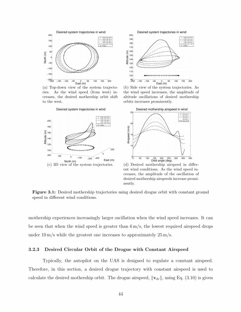
−200 −150 −100 −50 0 50 100 150 200−200
−150
−100
−50
0
50
100
150
200
Desired system trajectories in wind
East (m)
Nort
h (
m)
mshp: ||w||=2m/s
mshp: ||w||=4m/s
mshp: ||w||=6m/s
mshp: ||w||=8m/s
mshp: ||w||=10m/s
drogue
(a) Top-down view of the system trajecto-ries. As the wind speed (from west) in-creases, the desired mothership orbit shiftto the west.
−200 −150 −100 −50 0 50 100 150 20090
100
110
120
130
140
150
160
170
180
190
200
Desired system trajectories in wind
East (m)
Altitude (
m)
mshp: ||w||=2m/s
mshp: ||w||=4m/s
mshp: ||w||=6m/s
mshp: ||w||=8m/s
mshp: ||w||=10m/s
drogue
(b) Side view of the system trajectories. Asthe wind speed increases, the amplitude ofaltitude oscillations of desired mothershiporbits increases prominently.
−200
0
200
−200−1000100200
100
120
140
160
180
200
East (m)
Desired system trajectories in wind
North (m)
Altitude (
m)
mshp: ||w||=2m/s
mshp: ||w||=4m/s
mshp: ||w||=6m/s
mshp: ||w||=8m/s
mshp: ||w||=10m/s
drogue
(c) 3D view of the system trajectories.
0 50 100 150 200 250 300 350 4005
10
15
20
25
Desired mothership airspeed in wind
Orbit angle (deg)
Airspeed (
m/s
)
||w||=2m/s
||w||=4m/s
||w||=6m/s
||w||=8m/s
||w||=10m/s
(d) Desired mothership airspeed in differ-ent wind conditions. As the wind speed in-creases, the amplitude of the oscillation ofdesired mothership airspeeds increase promi-nently.
Figure 3.1: Desired mothership trajectories using desired drogue orbit with constant groundspeed in different wind conditions.
mothership experiences increasingly larger oscillation when the wind speed increases. It can
be seen that when the wind speed is greater than 6 m/s, the lowest required airspeed drops
under 10 m/s while the greatest one increases to approximately 25 m/s.
3.2.3 Desired Circular Orbit of the Drogue with Constant Airspeed
Typically, the autopilot on the UAS is designed to regulate a constant airspeed.
Therefore, in this section, a desired drogue trajectory with constant airspeed is used to
calculate the desired mothership orbit. The drogue airspeed, ‖vdr‖, using Eq. (3.10) is given
44

by
‖vdr‖ =
√(−rdrϕ sinϕ− wn)2 + (rdrϕ cosϕ− we)2 + w2
d. (3.11)
Therefore, given a desired drogue airspeed vadr, we have
r2drϕ2 + 2rdr (wn sinϕ− we cosϕ) ϕ+ w2
n + w2e + w2
d − (vadr)2 = 0. (3.12)
Solving the quadratic equation for ϕ, the clockwise motion is given by
ϕ =we cosϕ− wn sinϕ+
√(wn sinϕ− we cosϕ)2 −
(w2n + w2
e + w2d − (vadr)
2)rdr
. (3.13)
Figure 3.1 shows the desired mothership trajectories in different wind conditions
using a desired drogue orbit with constant airspeed by selecting vadr = 14 m/s, h0 = 100 m,
rddr = 120 m, and using a 85 m long, 5-link cable model. It can be seen from Fig. 3.1 (a)
that as the wind speed increases, the mothership orbit shifted to the west in the horizontal
direction, which is similar to the results in Fig. 3.0 (a). It can be seen from Fig. 3.1 (b)
that the amplitude of the oscillation of desired mothership orbits decreases compared with
Fig. 3.0 (b). The amplitude of the oscillation was no more than 5 m for wind speed 10 m/s.
Figure 3.1 (c) shows the variation trend of the desired mothership orbits in a 3D view.
Figure 3.1 (d) shows the desired airspeed of the mothership versus the orbit angle. It can be
seen that the amplitude of mothership’s airspeed oscillations also decreases compared with
Fig. 3.0 (d). It can be seen that the lowest required airspeed is greater than the nominal
desired airspeed of the drogue while the highest one increases to approximately 24 m/s.
For the purpose of implementation of the strategy of the drogue orbit control in the
flight test, the performance limits of the mothership need to be accounted for. Based on the
current hardware of the flight test, the airspeed range of the mothership is 10−20 m/s. Thus,
the mothership is able to follow the desired trajectory shown in Fig.3.1 in the presence of wind
whose speed is smaller than 7 m/s. To increase the capability of the mothership to follow
the desired trajectory in larger wind, the amplitudes of oscillations of desired mothership
airspeeds need to be decreased by changing the parameters of the desired drogue orbit.
Because the desired drogue airspeed is required to be the nominal airspeed of the MAV, the
45

−200 −150 −100 −50 0 50 100 150 200−200
−150
−100
−50
0
50
100
150
200
Desired system trajectories in wind
East (m)
Nort
h (
m)
mshp: ||w||=2m/s
mshp: ||w||=4m/s
mshp: ||w||=6m/s
mshp: ||w||=8m/s
mshp: ||w||=10m/s
drogue
(a) Top-down view of the system trajecto-ries. As the wind speed (from west) in-creases, the desired mothership orbit shiftto the west.
−200 −150 −100 −50 0 50 100 150 20090
100
110
120
130
140
150
Desired system trajectories in wind
East (m)
Altitude (
m)
mshp: ||w||=2m/s
mshp: ||w||=4m/s
mshp: ||w||=6m/s
mshp: ||w||=8m/s
mshp: ||w||=10m/s
drogue
(b) Side view of the system trajectories. Asthe wind speed increases, the amplitude ofaltitude oscillations of desired mothershiporbits increases insignificantly.
−200
−100
0
100
200
−200
−100
0
100
200
100
120
140
160
180
200
East (m)
Desired system trajectories in wind
North (m)
Altitude (
m)
mshp: ||w||=2m/s
mshp: ||w||=4m/s
mshp: ||w||=6m/s
mshp: ||w||=8m/s
mshp: ||w||=10m/s
drogue
(c) 3D view of the system trajectories.
0 50 100 150 200 250 300 350 40014
15
16
17
18
19
20
21
22
23
24
Desired mothership airspeed in wind
Orbit angle (deg)
Airspeed (
m/s
)
||w||=2m/s
||w||=4m/s
||w||=6m/s
||w||=8m/s
||w||=10m/s
(d) Desired mothership airspeed in differ-ent wind conditions. As the wind speed in-creases, the amplitude of the oscillation ofdesired mothership airspeeds increase promi-nently.
Figure 3.2: Desired mothership trajectories using desired drogue orbit with constant airspeedand orbit radius rddr = 120 m in different wind conditions.
desired orbit radius of the drogue needs to be increased so that amplitudes of oscillations
of the desired airspeed could decrease. Figure 3.2 shows the results using the desired orbit
radius of the drogue as rddr = 250 m. It can be seen that desired airspeeds of the mothership
remain in 14 − 18 m/s. Amplitudes of oscillations of the desired mothership altitude also
become smaller relative to Fig. 3.1 (b).
46

−400 −300 −200 −100 0 100 200 300 400−400
−300
−200
−100
0
100
200
300
400
Desired system trajectories in wind
East (m)
Nort
h (
m)
mshp: ||w||=2m/s
mshp: ||w||=4m/s
mshp: ||w||=6m/s
mshp: ||w||=8m/s
mshp: ||w||=10m/s
drogue
(a) Top-down view of the system trajecto-ries. As the wind speed (from west) in-creases, the desired mothership orbit shiftto the west.
−400 −300 −200 −100 0 100 200 300 40090
95
100
105
110
115
120
125
130
135
140
Desired system trajectories in wind
East (m)
Altitude (
m)
mshp: ||w||=2m/s
mshp: ||w||=4m/s
mshp: ||w||=6m/s
mshp: ||w||=8m/s
mshp: ||w||=10m/s
drogue
(b) Side view of the system trajectories.
−500
0
500
−400
−200
0
200
400100
110
120
130
140
East (m)
Desired system trajectories in wind
North (m)
Altitude (
m)
mshp: ||w||=2m/s
mshp: ||w||=4m/s
mshp: ||w||=6m/s
mshp: ||w||=8m/s
mshp: ||w||=10m/s
drogue
(c) 3D view of the system trajectories.
0 50 100 150 200 250 300 350 40015
15.5
16
16.5
17
17.5
18
Desired mothership airspeed in wind
Orbit angle (deg)
Airspeed (
m/s
)
||w||=2m/s
||w||=4m/s
||w||=6m/s
||w||=8m/s
||w||=10m/s
(d) Desired mothership airspeed in differ-ent wind conditions. As the wind speedincreases, amplitudes of oscillations of de-sired mothership airspeeds increase. Thelargest amplitude is smaller than that inFig. 3.1 (d).
Figure 3.3: Desired mothership trajectories using desired drogue orbit with constant airspeedand orbit radius rddr = 250m in different wind conditions .
3.3 Flight Test Results
In this section, an approach to convert the desired mothership trajectory into a series
of waypoints is developed. After that, a trajectory tracking method based on waypoint
following is introduced. The flight test results are presented to validate the applicability of
the motion planning and control strategies.
47

3.3.1 Waypoint Generation and Tracking
To implement the trajectory tracking for the mothership in the flight test, tradi-
tional controllers may be impractical because the autopilot can only take certain commands
as inputs. In this section, a strategy is developed to produce a series of waypoints with
corresponding airspeeds using the desired mothership trajectory.
Given the current position of the mothership, the procedure of computing the com-
manded waypoint is as follows:
1. Given a desired drogue orbit, the desired mothership trajectory can be numerically
calculated using the differential-flatness-based method. Selecting an appropriate fixed
step size in the calculation to guarantee the resulting mothership trajectory includes
more than 361 discrete points in one period of the mothership orbit.
2. The center of the desired mothership orbit can be calculated by averaging the coordi-
nates of selected points in Step 1.
3. The orbit angle ϕ of each selected point on the orbit with respect to the orbit center
can be calculated with round off and wrapped within [−180, 180] degree.
4. A look-up table can be established with ϕ ascending sorted in the first column. The
corresponding desired coordinates in three dimensions, and airspeeds are listed in the
successive columns.
5. Removing the rows with duplicates of ϕ, a look-up table with 361 rows ascending
sorted in ϕ can be obtained.
6. Given the current position of the mothership, its orbit angle ϕp can be calculated.
Define the orbit angle of the commanded waypoint as ϕc , ϕp + λδϕ, where λ = 1
signifies a clockwise orbit and λ = −1 signifies a counterclockwise orbit, and δϕ is a
constant integer defined as the offset of the orbit angle of the commanded waypoint
and the orbit angle of the current position. The offset integer δϕ is dependent by the
step size of the controller and communication frequency, and its value is determined
by trial and error.
48

0 50 100 150 200 250 300−300
−250
−200
−150
−100
−50
0
50
Side View of System Trajectory
East (m)
No
rth
(m
)
Desired MShip
Actual MShip
Desired Drogue
Actual Drogue
(a) Top-down view of the systems
0 50 100 150 200 250 30090
100
110
120
130
140
150
160
170
Side View of System Trajectory
East (m)
Altitu
de
(m
) Desired MShip
Actual MShip
Desired Drogue
Actual Drogue
(b) Side view of the systems
0 20 40 60 80 10012
14
16
18
20
Va (
m/s
)
MShip Airspeed and Altitude
CommandedActual
0 20 40 60 80 100130
140
150
160
170
Time (s)
Altitu
de
(m
)
(c) Airspeed and altitude of the mothership
0 20 40 60 80 100−2
0
2
Mothership Trajectory Tracking Error
Va (
m/s
)
0 20 40 60 80 100−10
0
10
No
rth
(m
)
0 20 40 60 80 100−10
0
10
Ea
st
(m)
0 20 40 60 80 100−10
0
10
Time (s)
Alt (
m)
(d) Tracking error of the mothership
0 20 40 60 80 10090
100
110
120
130
140
150
160
170
Mothership/Drogue Altitude vs Time
Time (s)
Altitu
de
(m
)
Mothership
Drogue
(e) Altitude evolutions of the mothership
0 20 40 60 80 100−4
−3.5
−3
−2.5
Nort
h (
m/s
)
GPS Wind Est in VC
0 20 40 60 80 100−2.5
−2
−1.5
Time (s)
East (m
/s)
(f) Wind estimation in North and East di-rections
Figure 3.4: Flight test results using the desired drogue orbit with constant ground speed.
49
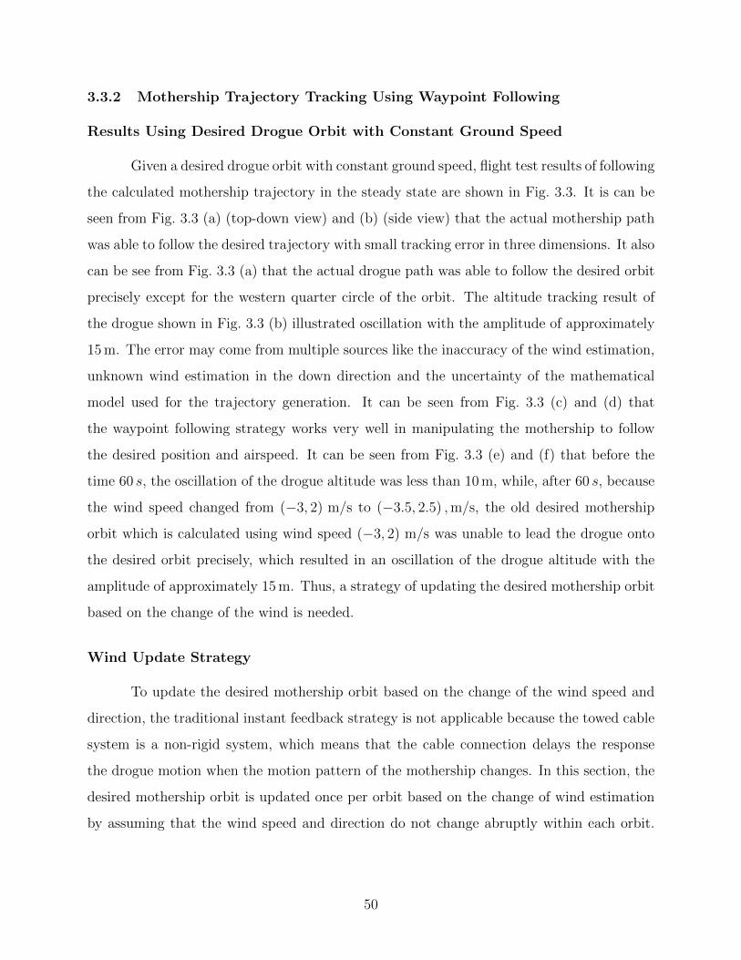
3.3.2 Mothership Trajectory Tracking Using Waypoint Following
Results Using Desired Drogue Orbit with Constant Ground Speed
Given a desired drogue orbit with constant ground speed, flight test results of following
the calculated mothership trajectory in the steady state are shown in Fig. 3.3. It is can be
seen from Fig. 3.3 (a) (top-down view) and (b) (side view) that the actual mothership path
was able to follow the desired trajectory with small tracking error in three dimensions. It also
can be see from Fig. 3.3 (a) that the actual drogue path was able to follow the desired orbit
precisely except for the western quarter circle of the orbit. The altitude tracking result of
the drogue shown in Fig. 3.3 (b) illustrated oscillation with the amplitude of approximately
15 m. The error may come from multiple sources like the inaccuracy of the wind estimation,
unknown wind estimation in the down direction and the uncertainty of the mathematical
model used for the trajectory generation. It can be seen from Fig. 3.3 (c) and (d) that
the waypoint following strategy works very well in manipulating the mothership to follow
the desired position and airspeed. It can be seen from Fig. 3.3 (e) and (f) that before the
time 60 s, the oscillation of the drogue altitude was less than 10 m, while, after 60 s, because
the wind speed changed from (−3, 2) m/s to (−3.5, 2.5) ,m/s, the old desired mothership
orbit which is calculated using wind speed (−3, 2) m/s was unable to lead the drogue onto
the desired orbit precisely, which resulted in an oscillation of the drogue altitude with the
amplitude of approximately 15 m. Thus, a strategy of updating the desired mothership orbit
based on the change of the wind is needed.
Wind Update Strategy
To update the desired mothership orbit based on the change of the wind speed and
direction, the traditional instant feedback strategy is not applicable because the towed cable
system is a non-rigid system, which means that the cable connection delays the response
the drogue motion when the motion pattern of the mothership changes. In this section, the
desired mothership orbit is updated once per orbit based on the change of wind estimation
by assuming that the wind speed and direction do not change abruptly within each orbit.
50

The desired mothership orbit is updated once the mothership crosses the half plane [88]
H (r,n) ,
pm ∈ R2 : (pm − r)T n ≥ 0,
where pm is the position of the mothership in the horizontal plane, r ∈ R2 and a normal
vector n ∈ R2 are used to define the position half plane. By selecting r = (−2, 0)T and
n = (0,−1)T , the half plane is defined as the plane which separates the third and forth
quadrant.
To facilitate the wind update during the flight test, the desired trajectories of the
mothership in different wind conditions were precalculated using different wind speeds with
the same assumed direction (from the west). Each time when the mothership crosses the half
plane, the desired mothership orbit is updated using the average wind update in the past
circle. When the actual wind direction is not along the assumed direction, the precalculated
mothership orbit will be rotated so that the desired mothership orbit corresponds to the
actual wind condition.
Results Using Desired Drogue Orbit with Constant Airspeed
To facilitate the air-to-air rendezvous for drogue and seeker UAS in the flight test,
a desired drogue orbit with constant airspeed and larger radius (250 m) was employed to
generate the desired mothership orbit so that the seeker has less curved path to follow and
the drogue has a relative stable airspeed which is easier for the seeker UAS to match.
Using the desired drogue orbit in Fig. 3.2 and the wind update strategy introduced
in the previous sub-section, Figure 3.4 shows the flight test results using a desired drogue
orbit with constant airspeed and a orbit radius of 250 m. The desired mothership orbit
was updated at time 20, 100, 180, 260 s. It can be seen from Fig. 3.4 (a) and (b) that the
actual mothership path was able to follow the desired trajectory with small tracking error in
three dimensions except for a deviation in the southwest corner. This deviation came from a
short delay in the communication between MATLAB/Simulink and VC. This phenomenon
sometimes happened when MATLAB/Simulink started for first time. The altitude tracking
result of the drogue shown in Fig. 3.3 (b) illustrated oscillation with an average amplitude
51

−500 −400 −300 −200 −100 0 100 200−400
−300
−200
−100
0
100
200
300
400
Side View of System Trajectory
East (m)
No
rth
(m
)
Desired MShip
Actual MShip
Desired Drogue
Actual Drogue
(a) Top-down view of the systems
−600 −500 −400 −300 −200 −100 0 100 20090
100
110
120
130
140
150
Side View of System Trajectory
East (m)
Altitu
de
(m
) Desired MShip
Actual MShip
Desired Drogue
Actual Drogue
(b) Side view of the systems
0 50 100 150 200 250 30013
14
15
16
17
Va (
m/s
)
MShip Airspeed and Altitude
Commanded
Actual
0 50 100 150 200 250 300130
135
140
145
150
Time (s)
Altitu
de
(m
)
(c) Airspeed and altitude of the mothership
0 50 100 150 200 250 300−2
0
2
Mothership Trajectory Tracking Error
Va (
m/s
)
0 50 100 150 200 250 300−200
0
200N
ort
h (
m)
0 50 100 150 200 250 300−100
0
100
Ea
st
(m)
0 50 100 150 200 250 300−10
0
10
Time (s)
Alt (
m)
(d) Tracking error of the mothership
0 50 100 150 200 250 30090
95
100
105
110
115
120
125
Drogue Altitude
Time (s)
Altitude (
m)
(e) Altitude evolutions of the mothership
0 50 100 150 200 250 3000.5
1
1.5
2
No
rth
(m
/s)
Wind Estimation
0 50 100 150 200 250 3003
3.2
3.4
3.6
3.8
Time (s)
Ea
st
(m/s
)
(f) Wind estimation in North and East di-rections
Figure 3.5: Flight test results using the desired drogue orbit with constant airspeed.
of approximately 10 m except for some large deviation. It can be seen from Fig. 3.4 (c) and
(d) that the waypoint following strategy works very well in manipulating the mothership to
follow the desired position and airspeed. It can be seen from Fig. 3.4 (d) that an obvious
52

deviation of the horizontal tracking happened at time period 50− 100 s, which corresponded
to the deviation in Fig. 3.4 (a) at the southwest corner. The reason could be the large wind
gust (see Fig. 3.4 (f)) and the inherent communication lag between the autopilot and the
combox in the multi-agent hardware structure. Figure 3.4 (e) shows that the amplitude of
the oscillation of the drogue altitude hold within 10m except for the large deviation at time
50− 100 s which matches the results in Fig. 3.4 (a) and (d). Figure 3.4 (f) shows the wind
estimation in north-east frame.
3.4 Conclusions
In this chapter, a trajectory generation algorithm based on differential flatness is
developed for the mothership to place the drogue onto a desired circular orbit. The equations
of motion of the cable are modified slightly to make the system dynamics differentially
flat. The numerical results are used to illustrate desired mothership trajectories and its
performance requirements like airspeed in different wind conditions using different desired
drogue trajectories. The resulting mothership trajectories using the desired drogue orbit
with constant airspeed and larger orbit radius express less requirement of the maneuver on
its airspeed and altitude. To implement the trajectory tracking in the flight test, an open-
loop waypoint following based approach was developed. The experimental results showed
that the waypoint following approach was satisfactory in tracking the commanded waypoints
and the airspeed. To take the wind change during the flight into consideration, a periodic
trajectory update strategy is developed to update the precalculated mothership trajectory
based on the wind prediction. The experimental results for the mothership to follow an orbit
with a large radius (250 m) with wind update showed that the mothership was able to lead
the drogue onto a desired orbit with the amplitude of the altitude oscillation less than 10 m
for 5 min.
53

Chapter 4
Optimal Trajectory Generation for the Mothership Using ModelPredictive Control
In the previous chapter, we introduced the trajectory generation algorithm using
differential flatness. The differential flatness based method is typically applied to the dis-
cretized model of the cable, and is computationally inexpensive compared to the optimal
control methods. However it requires the equations of motion of the system to be differen-
tially flat [77]. Another limitation is that this method does not directly take into account the
performance limitations of the system, so that the resulting trajectory of the towing vehicle
might be impractical. In particular, the resulting trajectories may violate constraint limits
on the manipulated variables (e.g. maximum available mothership thrust) or the controlled
variables (e.g. tension limitations of the cable).
Optimal control based methods were also used to generate the desired trajectory for
the towing vehicle [3, 4, 69, 71, 72]. Williams [3, 69] employed an optimal control method
to find a periodic path for the towing vehicle in order to minimize the motion of the towed
body subject to dynamic constraints. The problem was solved using sequential quadratic
programming. Williams et al. [4] used simulated annealing to solve the optimal control
problem in scheduling the orbit radius of the towing vehicle while the system transitions
from a straight flight into an orbit. Williams et al. [71] used optimal control in determining
the motion of the towing plane, as well as the cable deployment rate so that the towed
body passed through a set of desired waypoints. Williams [72] extended his work to find an
optimal elliptical orbit and cable deployment rate to compensate for crosswind disturbances.
Establishing an optimal motion of the towing vehicle subject to constraints using a
discretized multi-link cable model is a complicated optimization problem with many states
and degrees of freedom. However, discussions of the computational burden were seldom
54

mentioned. The typical algorithm used in solving the problem are based on quadratic pro-
gramming in which squared-error objectives are used. In this chapter, an approach based
on Model Predictive Control (MPC) using the L1-norm and squared error objectives are
introduced and applied to perform the optimal trajectory generation of the towing vehicle.
MPC with linear models [94–96] has been widely used in industrial applications such
as chemical plants and refineries [96]. Model predictive controllers rely on dynamic models
of the process, most often linear empirical models obtained by system identification. Be-
cause many of these processes have either semi-batch characteristics or nonlinear behavior,
the linear models are retrofitted with elements that approximate nonlinear control charac-
teristics to ensure that the linear models are applicable over a wider range of operating
conditions and disturbances. Some of the nonlinear process can be controlled by including
gain scheduling, switching between multiple models depending on operating conditions, and
other logical programming. Recent developments have permitted the direct application of
nonlinear models in control applications [97].
Various types of linear models are used for linear MPC applications including finite
impulse response, discrete or continuous state space, and Laplace domain functions. When
dealing with nonlinear systems, practitioners have attempted to extend linear models through
collections of piecewise linear models or linear time varying models. The linear models adapt
with either time or as a function of the current state of the system. A more general form
that is not dependent on model switching is collections of DAEs in open equation format.
These equations may include equality or inequality constraints, integer variables, and differ-
ential elements. To apply DAEs to nonlinear models, different approaches have been stud-
ied and implemented in the literature, including simultaneous methods [98], decomposition
methods [99, 100], efficient nonlinear programming solvers [101], improved estimation tech-
niques [102–105], and large-scale techniques for applications to industrial systems [106, 107].
The objective function used in the control optimization problems are typically based on a
weighted squared error or an L2-norm form. A common challenge with real measured values
is sensitivity to data outliers; the sensitivity to outliers is exacerbated by the squared error
norm.
55

One novel contribution of this chapter is a new L1-norm objective function for the
optimal control problem. These objective forms have a number of advantages over traditional
squared-error or L2-norm objectives. The L1-norm form is less sensitive to data outliers and
better rejects measurement noise. As mentioned previously, many of the remaining challenges
associated with implementing nonlinear models are due to the complexity of the numerical
solution techniques and commercial and academic software has been developed to meet this
challenge. This project uses the APMonitor Modeling Language [108] to model and solve
the large-scale DAE system of equations. Filtered bias updating, Kalman filtering, Moving
Horizon Estimation (MHE) and nonlinear MPC can be implemented in this web-services
platform through interfaces to MATLAB or Python. In this paper, the optimal control
problem of generating a desired trajectory for the mothership with performance limits to
place the drogue trajectory onto a desired orbit will be solved by using a nonlinear MPC
method. We utilize a combination objective functions in which a squared-error objective
form is used in calculating the trajectory tracking error and L1-norm objectives are used in
regulating the constraints.
The remainder of the chapter is structured as follows. Section 4.1 introduces the
formulation of nonlinear MPC and the combined objective function used in generating a
constrained optimal trajectory for the mothership. Section 4.2 shows the numerical results
of the optimal trajectory generation of the mothership using various desired drogue motions.
4.1 MPC Formulation
Given a desired trajectory for the drogue (e.g., a level circular orbit), a strategy is
needed to generate a mothership trajectory that produces the desired drogue path. Dif-
ferential flatness has been used in the trajectory generation of the towed cable system
in [2, 15, 18, 68] by applying certain types of dynamic models of the cable. For the math-
ematical model presented in Chapter 2, it is nontrivial to calculate the desired mothership
trajectory by using differential flatness. In addition, since the mothership has performance
limits like airspeed, roll angle, and climbing rate, differential flatness based methods do not
directly take these constraints into consideration. Furthermore, during transitions between
56

straight and level flight and orbital flight, the tension forces exerted on the cable should not
exceed the loading limit of the cable.
In this section, we will introduce a strategy to produce an optimal trajectory for the
mothership to place the drogue onto the desired orbit in the presence of system constraints.
In the literature, when formulating the optimal control problem for generating the desired
mothership trajectory, the nonlinear kinematic or dynamic models of the mothership were
typically used, and the objective functions were usually based on squared error or L2-norm
form. In this section, to reduce the computation time, we use linear dynamic equations of
the mothership and a novel format of the objective function to formulate the MPC problem.
Letting vm ∈ R3 be the mothership velocity relative to the wind frame, wc be the
constant component of the wind expressed in the inertial frame, and am ∈ R3 be the moth-
ership acceleration in the inertial frame, which is selected as the input of the mothership
dynamic, the equations of motion for the mothership are given by
pm = vm + wc, (4.1)
vm = am. (4.2)
The performance constraints of the mothership are typically given by the magnitude of the
mothership airspeed Va, the heading angle ψ, the bank angle φ, and the air mass referenced
flight path angle γa, which is defined as the angle from the inertial north-east plane to the
velocity vector of the aircraft relative to the air mass. The kinematic equations of motion
for the mothership are written as [88]
pn = Va cosψ cos γa + wn, (4.3)
pe = Va sinψ cos γa + we, (4.4)
pd = −Va sin γa + wd, (4.5)
ψ =g
Vatanφ. (4.6)
57

By comparing Eqs. (4.1) and (4.2), the constrained variables can be expressed as
Va = ‖vm‖ ,
ψ = tan−1(
vm (2)
vm (1)
),
γa = − sin−1(
vm (3)
Va
),
ψ =am (2) vm (1)− am (1) vm (2)
‖vm‖2,
φ = tan−1(Vagψ
).
Letting pddr (t) ∈ R3 be the desired drogue trajectory, pdr (t) ∈ R3 be the actual
drogue trajectory, Φ ∈ R be the objective function value, y , (y0, · · · , yn)T ∈ Rn be the
controlled variables, yhi, ylo ∈ Rn be the higher and lower dead-bands of the controlled
variables, whi, wlo ∈ Rn be the weights on the controlled variables outside the dead-bands,
u ∈ Rn be the inputs, cy, cu ∈ Rn are cost weights of y and u, f : Rn → Rn represent the
equations of motion, x ∈ Rn be the states of the equations of motion, d ∈ Rn be parameters
or unmeasured disturbances, giec : Rn → Rn represent the inequality constraints, τ ∈ R be
the response time constant of the desired controlled variables, sphi, splo ∈ Rn be dead-band
setpoints, and ehi and elo be slack variables 1 selected by the optimizer to penalize y above
and below the dead-band, and given by
ehi,i =
yi − yhi,i yi − yhi,i ≥ 0
0 yi − yhi,i < 0
, and elo,i =
ylo,i − yi ylo,i − yi ≥ 0
0 ylo,i − yi < 0
, i = 1, · · ·n,
1http://apmonitor.com/wiki/index.php/Main/SlackVariables
58

then the trajectory generation problem can be posed as the following optimization problem:
minu(t0,t1)
Φ = wThiehi + wT
loelo + yTcy + uTcu
+
∫ t1
t0
(pdr (δ)− pddr (δ)
)T (pdr (δ)− pddr (δ)
)dδ, (4.7a)
s.t. f (x,x,y,u,d) = 0, (4.7b)
giec (x,x,y,u,d) > 0, (4.7c)
τ∂yhi∂t
+ yhi = sphi, (4.7d)
τ∂ylo∂t
+ ylo = splo. (4.7e)
A combination of L1-norm and squared-error objectives, shown in Eq. (4.7a), is used
to accomplish multiple objectives. The controlled variables y are selected as the constraints
of the system. The L1-norm objective was used to regulate high-priority constraints like the
cable tension and the airspeed of the mothership. In this case, the controlled variables were
not forced to follow a desired trajectory, but were constrained to remain within certain range
of acceptable limits. The slack variables ehi and elo are then used to regulate y to remain
within dynamic dead-bands parametrized by yhi and ylo. The squared-error (integration)
term was used to penalize the trajectory tracking error of the drogue with a lower weighting
that represented the lower priority of the tracking objective. Eqs. (4.7b) and (4.7c) are
used to regulate the states to satisfy the equations of motion and some other inequality
constraints.
Eqs. (4.7d) and (4.7e) are linear first order equations that define the regulations for
controlled variables represented by either a dead-band or reference trajectory to the setpoints.
The setpoints sphi and splo are used to define regions that are not penalized in the objective
function and are referred to as the “dead-band”. It is desirable to make the evolution of
the controlled variables effectively approach setpoints at a specified rate so that excessive
movements of manipulated variables or response overshoots of controlled variables can be
avoided. Based on different control objectives, the initial conditions of yhi and ylo, can be set
to give a wider dead-band at the beginning of the simulation and only to enforce the steady
59

state response (and vice versa). Different initial conditions defining a wide or narrow dead-
band are the trade-off between precise steady-state response and precise dynamic evolution.
Therefore, reference trajectories of y by specifying the values of sphi and splo can be a step,
ramp or other dynamic signals.
4.2 Numerical Results
In this section, we use the MPC strategy described in Section 4.1 to compute open-
loop mothership trajectories, for a variety of desired drogue trajectories. The performance
limits of the mothership are selected as ψ ∈ [−0.35, 0.35] rad/s, Va ∈ [10, 20] m/s and γa ∈
[−0.35, 0.35] rad. The MPC problem was solved using APMonitor Modeling Language [108].
A step size of 2 seconds was selected as a compromise between the computation time and
the accuracy of the results. The computer used to solve the optimization problem has an
AMD 64 core processor with 64 GB of RAM.
4.2.1 Desired Drogue Orbit with Constant Ground Speed
In the final phase of the aerial recovery scenario, the drogue must be placed onto an
orbit that can be easily followed by the MAV. In this section, the desired drogue trajectory
is a constant altitude circular orbit with constant ground speed. Let rddr be the desired
constant orbit radius of the drogue, ϕ (t) be the orbital angle of the orbit measured from
the north, and h0 be the desired constant altitude of the drogue, the desired circular orbit
of the drogue in three dimensions is given by
pddrn (t) = rddr cosϕ (t) , (4.8)
pddre (t) = rddr sinϕ (t) , (4.9)
pddrd (t) = −h0. (4.10)
Letting vgdr be the desired constant ground speed of the drogue, the orbit angle for a clockwise
motion can be written as ϕ (t) = vgdrt/rdr. Without loss of generality, the wind is assumed
from the west direction. A typical circular orbit for drogue can be parametrized by selecting
vgdr = 12 m/s, h0 = 100 m, rddr = 100 m, and the orbit period can be calculated by T gp =
60

Table 4.1: Solution results using the desired drogue orbit with constant ground speed
Wind speed (m/s) p0m (m) v0
m (m/s) Solution Time (s) Φ
0 (−79, 90,−157) (−10,−8, 0) 18.4 0.1
(0, 5, 0)T (−67, 55,−157) (−9.4,−7.3, 2) 17.1 0.2
(0, 10, 0)T (−61, 35,−142) (−9,−5, 2) 48.1 7965.1p0m = initial mothership position; v0
m = initial mothership velocity in NED frame.
2πrddr/vgdr = 52.36 s. The starting and end clocks are selected as t0 = 0 and t1 = 70 s, so that
the resulting mothership trajectory has enough waypoints to produce an orbit. The optimal
control solver is selected as IPOPT [109], which is an open-source Interior Point solver
for solving nonlinear programming (NLP) problems included with the COIN-OR collection.
The initial configuration and solution results are shown in Table 4.0. It can be seen that the
objective function values were less than 0.5 when the wind speeds were less than 5 m/s, and
increased to approximately 8000 when the wind speed increased to 10 m/s. This is because
the existing performance limits of the mothership made the resulting optimal orbit unable
to precisely place the drogue orbit onto the desired orbit.
−200−100
0100
200
−200
−100
0
100
20080
100
120
140
160
180
East (m)
System trajectory
North (m)
Altitude (
m)
Drogue
Mothership
Desired drogue
Cable
(a) 3-D view.
−150 −100 −50 0 50 100 150−150
−100
−50
0
50
100
150
East (m)
Nort
h (
m)
System trajectory
Drogue
Mothership
Desired drogue
Cable
(b) Top-down view.
−200−150−100−5005010015020090
100
110
120
130
140
150
160
170
System trajectory
North (m)
Altitude (
m)
Drogue
Mothership
Desired drogue
Cable
(c) Side view.
Figure 4.1: Optimal system trajectories in the absence of wind. A horizontally flat desireddrogue orbit (triangle-dot line) resulted in a desired horizontally flat mothership orbit (dash-dot line). The actual drogue trajectory (dashed line) follows the desired orbit precisely. Thecable (solid line) curved because of the aerodynamic forces exerted on the joint.
Figure 4.0 shows the different views of optimal system trajectories in the absence
of wind. It can be seen that a horizontally flat desired drogue orbit resulted in a desired
61

−200−100
0100
−200−100
0100
20050
100
150
200
East (m)
System trajectory
North (m)
Altitude (
m)
Drogue
Mothership
Desired drogue
Cable
(a) 3-D view.
−200 −150 −100 −50 0 50 100−150
−100
−50
0
50
100
150
East (m)
Nort
h (
m)
System trajectory
Drogue
Mothership
Desired drogue
Cable
(b) Top-down view.
−200−150−100−5005010015020090
100
110
120
130
140
150
160
170
180
190
System trajectory
North (m)
Altitude (
m)
Drogue
Mothership
Desired drogue
Cable
(c) Side view.
Figure 4.2: Optimal system trajectories using a desired drogue orbit with constant groundspeed in the presence of 5 m/s wind from the west. A horizontally flat desired drogue orbit(triangle-dot line) resulted in an inclined desired mothership orbit (dash-dot line). The centerof the mothership orbit shifted to the west of the center of the drogue orbit. The amplitude ofthe mothership’s altitude oscillation was approximately 40 m.
0 10 20 30 40 50 60 705
10
15
20
25
Time (s)
Va (
m/s
)
Airspeed
Va
Dead−bands
(a) Airspeed Va vs. time.
0 10 20 30 40 50 60 70−0.5
−0.4
−0.3
−0.2
−0.1
0
0.1
0.2
0.3
0.4
0.5
Time (s)
γa (
rad)
Flight path angle
γa
Dead−bands
(b) Flight path angle (γa) vs.time.
0 10 20 30 40 50 60 70−0.5
−0.4
−0.3
−0.2
−0.1
0
0.1
0.2
0.3
0.4
0.5
Time (s)
ψ r
ate
(ra
d/s
)
Heading rate
ψ rate
Dead−bands
(c) Heading rate ψ vs. time.
Figure 4.3: Evolution of constrained variables of the mothership using a desired drogue orbitwith constant ground speed in the presence of 5 m/s wind from the west. All the variablevalues (solid lines) remained within their limits (dashed lines).
horizontally flat mothership orbit. Figure 4.1 shows the different views of the optimal system
trajectories in the presence of 5 m/s wind from the west. It can be seen that the desired
mothership orbit is inclined to produce a horizontally flat orbit of the drogue in the presence
of wind. The amplitude of the mothership’s altitude oscillation was approximately 40 m.
Figure 4.2 shows the evolutions of the constraints variables Va, γa and ψ of the mothership.
It can be seen that all the variables remained within the constraints. Figure 4.3 shows
the different views of the optimal system trajectories in the presence of 10 m/s wind from
the west. It can be seen that the desired mothership orbit inclines more in a stronger
62

−200
0
200
−200−100
0100
20050
100
150
200
East (m)
System trajectory
North (m)
Altitude (
m)
Drogue
Mothership
Desired drogue
Cable
(a) 3-D view.
−200 −150 −100 −50 0 50 100 150−150
−100
−50
0
50
100
150
East (m)
Nort
h (
m)
System trajectory
Drogue
Mothership
Desired drogue
Cable
(b) Top-down view.
−200−150−100−5005010015020080
100
120
140
160
180
200
System trajectory
North (m)
Altitude (
m)
Drogue
Mothership
Desired drogue
Cable
(c) Side view.
Figure 4.4: Optimal system trajectories using a desired drogue orbit with constant groundspeed in the presence of 10 m/s wind from the west. The resulting optimal mothership orbit(dash-dot line) was unable to place the actual drogue trajectory (dashed line) onto the desiredorbit (triangle-dot line) precisely because of the performance limits. The amplitude of themothership’s altitude oscillation was approximately 70 m, while the amplitude of the drogue’saltitude oscillation was approximately 15 m.
0 10 20 30 40 50 60 705
10
15
20
25
Time (s)
Va (
m/s
)
Airspeed
Va
Dead−bands
(a) Airspeed Va vs. time.
0 10 20 30 40 50 60 70−0.5
−0.4
−0.3
−0.2
−0.1
0
0.1
0.2
0.3
0.4
0.5
Time (s)
γa (
rad)
Flight path angle
γa
Dead−bands
(b) Flight path angle γa vs. time.
0 10 20 30 40 50 60 70−0.5
−0.4
−0.3
−0.2
−0.1
0
0.1
0.2
0.3
0.4
0.5
Time (s)
ψ r
ate
(ra
d/s
)
Heading rate
ψ rate
Dead−bands
(c) Heading rate ψ vs. time.
Figure 4.5: Evolution of constrained variables of the mothership using a desired drogue orbitwith constant ground speed in the presence of 10 m/s wind from the west. All variables(solid lines) reached the limits (dashed lines) during the simulation. The optimizer was ableto produce an optimal trajectory for the mothership by keeping all the constrained variableswithin their limits.
wind. Because of the performance limits of the mothership, the resulting optimal orbit was
unable to precisely place the drogue orbit onto the desired orbit, which results in a large
value for the objective function in Table 4.0. The amplitude of the mothership’s altitude
oscillation was approximately 70 m, while the amplitude of the drogue’s altitude oscillation
was approximately 15 m. Figure 4.4 shows the evolutions of the constraints Va, γa and ψ
of the mothership. It can be seen that although all the constrained variables reached their
63

limits during the flight, the optimizer was able to produce an optimal trajectory for the
mothership to place the drogue orbit to essentially follow the desired orbit.
4.2.2 Desired Drogue Orbit with Constant Airspeed
Because the autopilot on the MAV is typically designed to regulate a constant air-
speed, in this section, a desired drogue trajectory with constant airspeed is used to calculate
the desired mothership orbit. The time derivative of pddr (t) using Eqs. (4.8) to (4.10) is given
by
pddr =
−rddrϕ sinϕ
rddrϕ cosϕ
0
= vsdr + w. (4.11)
Using Eqs. (3.11)-(3.13), we can obtain a drogue orbit with constant airspeed. The orbital
period T ap can be calculated by [72]
T ap =
∫ 2π
0
1
ϕdϕ. (4.12)
It is not difficult to see that T ap increases when the wind speed increases. In the presence of
5 m/s wind, T ap can be calculated as 60.51 s by using Eq. (4.12). When the wind increases to
10 m/s, T ap increases to 135.8 s. To guarantee that the optimal trajectory of the mothership
has enough waypoints to produce an orbit, the starting and end times are selected as t0 = 0
and t1 = 70 s for the case of 5 m/s wind, and t1 = 150 s for the case of 10 m/s wind. The
initial configuration and solution results are shown in Table 4.1. It can be seen that when
the wind speed increased to 10 m/s, the objective function value increased to 755.2. This is
because the existing performance limits of the mothership made the resulting optimal orbit
unable to precisely place the drogue orbit onto the desired orbit. The parameters of the
desired drogue orbit were selected as rdr = 100 m and vadr = 12 m/s to compare the results
with those in the previous section.
Figure 4.5 shows the different views of the optimal system trajectories in the presence
of 5 m/s wind from the west. It can be seen that the offset of the mothership orbit center in
Fig. 4.5 (b) is smaller than the one in Fig. 4.1 (b). It also can be seen that the inclination
64

Table 4.2: Solution results using the desired drogue orbit with constant airspeed
Wind speed (m/s) p0m (m) v0
m (m/s) Solution Time (s) Φ
(0, 5, 0)T (−74, 63,−159) (−6,−9, 0) 18.8 17.9
(0, 10, 0)T (−20, 40,−159) (−3,−4, 0) 39.8 755.2p0m = initial mothership position; v0
m = initial mothership velocity in NED frame.
of the mothership orbit in Fig. 4.5 (c) was much smaller than the one in Fig. 4.1 (c). The
amplitude of the mothership’s altitude oscillation was approximately 10 m. Because the
desired airspeed of the drogue was constant, it can be seen that the waypoints placed close
together when the system is flying upwind (towards the west), and sparsely when the system
was flying downwind (towards the east). Figure 4.6 shows the evolutions of the constrained
variables Va, γa and ψ of the mothership. It can be seen that the desired airspeed of
mothership in Fig. 4.6 (a) reached its upper limit, while in the same wind condition, the
desired airspeed in Fig. 4.2 (a) was still within the limits.
−200−100
0100
200
−200
−100
0
100
20080
100
120
140
160
180
East (m)
System trajectory
North (m)
Altitude (
m)
Drogue
Mothership
Desired drogue
Cable
(a) 3-D view.
−200 −150 −100 −50 0 50 100 150−150
−100
−50
0
50
100
150
East (m)
Nort
h (
m)
System trajectory
Drogue
Mothership
Desired drogue
Cable
(b) Top-down view.
−200−150−100−5005010015020090
100
110
120
130
140
150
160
170
System trajectory
North (m)
Altitude (
m)
Drogue
Mothership
Desired drogue
Cable
(c) Side view.
Figure 4.6: Optimal system trajectories using a desired drogue orbit with constant airspeedin the presence of 5 m/s wind from the west. The resulting optimal mothership orbit (dash-dotline) was larger than the one in Fig. 4.1. The amplitude of the mothership’s altitude oscillationwas approximately 10 m, which was much smaller than the one in Fig. 4.1. The waypointsplaced close together when the system was flying upwind (towards the west), and sparse whenthe system was flying downwind (towards the east).
Figure 4.7 shows the different views of the optimal system trajectories in the presence
of 10 m/s wind from the west. It can be seen that the offset of the mothership orbit center
and the inclination of the desired mothership orbit become larger than those in Fig. 4.5. The
65

0 10 20 30 40 50 60 705
10
15
20
25
Time (s)
Va (
m/s
)Airspeed
Va
Dead−bands
(a) Airspeed Va vs. time.
0 10 20 30 40 50 60 70−0.5
−0.4
−0.3
−0.2
−0.1
0
0.1
0.2
0.3
0.4
0.5
Time (s)
γa (
rad)
Flight path angle
γa
Dead−bands
(b) Flight path angle γa vs. time.
0 10 20 30 40 50 60 70−0.5
−0.4
−0.3
−0.2
−0.1
0
0.1
0.2
0.3
0.4
0.5
Time (s)
ψ r
ate
(ra
d/s
)
Heading rate
ψ rate
Dead−bands
(c) Heading rate ψ vs. time.
Figure 4.7: Evolution of constrained variables of the mothership using a desired drogue orbitwith constant airspeed in the presence of 5 m/s wind from the west. All the constrainedvariables (solid lines) remained within their limits (dashed lines) except for the airspeed.
−200−100
0100
200
−200
−100
0
100
20080
100
120
140
160
180
East (m)
System trajectory
North (m)
Altitude (
m)
Drogue
Mothership
Desired drogue
Cable
(a) 3-D view.
−200 −150 −100 −50 0 50 100 150−150
−100
−50
0
50
100
150
East (m)
Nort
h (
m)
System trajectory
Drogue
Mothership
Desired drogue
Cable
(b) Top-down view.
−200−150−100−5005010015020090
100
110
120
130
140
150
160
170
180
System trajectory
North (m)
A
ltitude (
m)
Drogue
Mothership
Desired drogue
Cable
(c) Side view.
Figure 4.8: Optimal system trajectories using a desired drogue orbit with constant airspeedin the presence of 10 m/s wind from the west. The amplitude of the mothership’s altitudeoscillation was approximately 20 m. The waypoints placed close together when the system wasflying upwind (towards the west), and sparse when the system was flying downwind (towardsthe east).
resulting drogue orbit shows both horizontal and vertical offsets, which imply the constrained
variables of the mothership reached their limits during the flight. The mothership trajectory
in Fig. 4.7 (c) may look unsmooth, but this is simply an effect of quantifying the trajectory
waypoints. Figure 4.8 shows the evolutions of the constrained variables Va, γa and ψ of the
mothership. It can be seen that the desired airspeed of the mothership reached the limit,
while γa and ψ still remained within their limits.
66

0 50 100 1505
10
15
20
25
Time (s)
Va (
m/s
)Airspeed
Va
Dead−bands
(a) Airspeed Va vs. time.
0 50 100 150−0.5
−0.4
−0.3
−0.2
−0.1
0
0.1
0.2
0.3
0.4
0.5
Time (s)
γa (
rad)
Flight path angle
γa
Dead−bands
(b) Flight path angle γa vs. time.
0 50 100 150−0.5
−0.4
−0.3
−0.2
−0.1
0
0.1
0.2
0.3
0.4
0.5
Time (s)
ψ r
ate
(ra
d/s
)
Heading rate
ψ rate
Dead−bands
(c) Heading rate ψ vs. time.
Figure 4.9: Evolution of constrained variables of the mothership using a desired drogue orbitwith constant airspeed in the presence of 10 m/s wind from the west. All the constrainedvariables (solid lines) were within their limits (dashed lines) except for the airspeed, which wasat the upper limit for a fraction of the trajectory.
4.2.3 Transitions between Straight Level Flight and Orbital Flight
The transition between a straight and level flight and orbital flight (and vice versa)
needs special attention for a towed cable system because the cable may become slack when the
mothership turns and may experience large and sudden forces that may break the cable [4].
To prevent the tension forces exerted on the cable exceeding the loading limit of the cable, an
optimal trajectory of the mothership is needed to keep the tension forces within their limits
during the transition. In this section, we focus on the tow-in motion in which the system flies
from a straight flight into an orbit. The tension forces on the cable are selected as additional
constraints in the optimization with the limits ‖Ti‖ ∈ [0, 10] N, i = 1, 2. Optimal results in
different wind conditions are presented in this section.
Letting ta be the time when transition started, the desired drogue trajectory in a
tow-in motion can be written as
(1) when t ∈ [0, ta], the straight-line trajectory of the drogue is given by
pddrn (t) = −vgdrt,
pddre (t) = rddr,
pddrd (t) = −h0;
67

(2) when t ∈ (ta, t1], the circular trajectory of the drogue is given by
pddrn (t) = −vgdrta + rddr cosϕ (t) ,
pddre (t) = rddr sinϕ (t) ,
pddrd (t) = −h0.
In this section, we use the desired circular drogue orbit with constant ground speed, i.e.,
ϕ (t) = vgdrt/rddr. We select rdr = 100 m, vgdr = 12 m/s, ta = 20 s and t1 = 80 s in the
optimization algorithm. The initial configuration and solution results are shown in Table 4.2.
It can be seen that the solution times under different wind conditions were less than 30 s,
while larger than those in Table 4.0 because a larger t1 was selected. When the wind
increased to 10 m/s, the objective function value increased to 1751. This is because the
existing performance limits of the mothership made the resulting optimal orbit unable to
precisely place the drogue orbit onto the desired orbit.
Table 4.3: Solution results of transitional flight in different wind conditions
Wind speed (m/s) p0m (m) v0
m (m/s) Solution Time (s) Φ
0 (−80, 100,−155) (−14, 0, 0) 23.2 20.3
(0, 5, 0)T (−80, 67,−155) (−14, 0, 0) 20.1 21.6
(0, 10, 0)T (−70, 41,−143) (−14, 0, 0) 29.7 1751.0p0m = initial mothership position; v0
m = initial mothership velocity in NED frame.
Figure 4.9 shows the different views of the optimal system trajectories during a tow-
in maneuver in the absence of wind. It can be seen that it takes one quarter circle for
the mothership to complete the transition. The mothership trajectory had an altitude os-
cillation of approximately 20 m during the transition. Figure 4.10 shows the evolutions of
the constrained variables Va, γa and ψ of the mothership. It can be seen that the airspeed
reached its lower limits during the transition. The large oscillation of γa explained the al-
titude oscillation of the mothership during the transition. Figure 4.11 shows the evolution
68

of the tension forces on the cable in the transitional flight. The tension forces had a small
oscillation (approximately 1 N), while remaining within their limits.
−200−100
0100
200
−400
−300
−200
−100
080
100
120
140
160
180
East (m)
System trajectory
North (m)
Altitude (
m)
Drogue
Mothership
Desired drogue
Cable
(a) 3-D view.
−150 −100 −50 0 50 100 150−400
−350
−300
−250
−200
−150
−100
−50
0
East (m)
Nort
h (
m)
System trajectory
Drogue
Mothership
Desired drogue
Cable
(b) Top-down view.
−400−350−300−250−200−150−100−50090
100
110
120
130
140
150
160
170
180
System trajectory
North (m)
Altitude (
m)
Drogue
Mothership
Desired drogue
Cable
(c) Side view.
Figure 4.10: Optimal system trajectories in the transitional flight in the absence of wind.The mothership trajectory (dash-dot line) had an obvious altitude oscillation (approximately20 m) during the transition and converged quickly to the desired orbit which place the droguetrajectory (dashed line) into the desired orbit (triangle-dot line).
0 10 20 30 40 50 60 70 805
10
15
20
25
Time (s)
Va (
m/s
)
Airspeed
Va
Dead−bands
(a) Airspeed Va vs. time.
0 10 20 30 40 50 60 70 80−0.5
−0.4
−0.3
−0.2
−0.1
0
0.1
0.2
0.3
0.4
0.5
Time (s)
γa (
rad)
Flight path angle
γa
Dead−bands
(b) Flight path angle γa vs. time.
0 10 20 30 40 50 60 70 80−0.5
−0.4
−0.3
−0.2
−0.1
0
0.1
0.2
0.3
0.4
0.5
Time (s)
ψ r
ate
(ra
d/s
)
Heading rate
ψ rate
Dead−bands
(c) Heading rate ψ vs. time.
Figure 4.11: Evolution of constrained variables of the mothership in the transitional flightin the absence of wind. The airspeed and flight path angle reached their limits during thetransition.
Figure 4.12 shows the different views of the optimal system trajectories during a
tow-in maneuver in the presence of 5 m/s wind from the west. It can be seen that the moth-
ership trajectory had an altitude oscillation of approximately 15 m during the transition.
69

0 10 20 30 40 50 60 70 80
0
2
4
6
8
10
12
14
Time (s)T
esio
n (
N)
Tension force
T1
T2
Dead−bands
Figure 4.12: Evolution of the tension forces of the cable in the transitional flight in theabsence of wind. The tension forces of the cable had a small oscillation during the transition,while they remained within their limits.
−200−100
0100
200
−400
−300
−200
−100
050
100
150
200
East (m)
System trajectory
North (m)
Altitude (
m)
Drogue
Mothership
Desired drogue
Cable
(a) 3-D view.
−200 −150 −100 −50 0 50 100 150−400
−350
−300
−250
−200
−150
−100
−50
0
East (m)
Nort
h (
m)
System trajectory
Drogue
Mothership
Desired drogue
Cable
(b) Top-down view.
−400−350−300−250−200−150−100−50090
100
110
120
130
140
150
160
170
180
190
System trajectory
North (m)
Altitude (
m)
Drogue
Mothership
Desired drogue
Cable
(c) Side view.
Figure 4.13: Optimal system trajectories in the transitional flight in the presence of 5 m/swind from the west. The resulting optimal mothership orbit (dash-dot line) had a offset tothe west of the drogue trajectory during the straight flight, experienced an altitude oscillationwith amplitude of approximately 15 m during the transition, and converged to the desired orbitwhich place the drogue trajectory (dashed line) into the desired orbit (triangle-dot line).
Figure 4.13 shows the evolutions of the constrained variables Va, γa and ψ of the mother-
ship. It can be seen that all the variables remained within the limits during the transition.
Figure 4.14 shows the cable tension evolution during the transitional flight. It can be seen
that the tension forces had an oscillation of approximately 2 N during the transition while
they still remained within the limits.
Figure 4.15 shows the different views of the optimal system trajectories during a
tow-in maneuver in the presence of 10 m/s wind from the west. It can be seen that the
mothership trajectory had an altitude oscillation of approximately 10 m during the transition.
70

0 10 20 30 40 50 60 70 805
10
15
20
25
Time (s)
Va (
m/s
)Airspeed
Va
Dead−bands
(a) Airspeed Va vs. time.
0 10 20 30 40 50 60 70 80−0.5
−0.4
−0.3
−0.2
−0.1
0
0.1
0.2
0.3
0.4
0.5
Time (s)
γa (
rad)
Flight path angle
γa
Dead−bands
(b) Flight path angle γa vs. time.
0 10 20 30 40 50 60 70 80−0.5
−0.4
−0.3
−0.2
−0.1
0
0.1
0.2
0.3
0.4
0.5
Time (s)
ψ r
ate
(ra
d/s
)
Heading rate
ψ rate
Dead−bands
(c) Heading rate ψ vs. time.
Figure 4.14: Evolution of constrained variables of the mothership in the transitional flight inthe presence of 5 m/s wind from the west. All the variables remained within their limits. Thelarge oscillation of the flight path angle (15 s to 30 s) explains the oscillation of the mothershipaltitude during the transition.
0 10 20 30 40 50 60 70 80
0
2
4
6
8
10
12
14
Time (s)
Tesio
n (
N)
Tension force
T1
T2
Dead−bands
Figure 4.15: Evolution of the tension forces of the cable in the transitional flight in thepresence of 5 m/s wind from the west. The tension forces of the cable had a small oscillationduring the transition, while they remained within their limits.
Figure 4.16 shows the evolutions of the constrained variables Va, γa and ψ of the mothership.
It can be seen that Va reached its upper bound while γa and ψ remained within the limits
during the transition. Therefore, the resulting optimal orbit unable to precisely place the
drogue orbit onto the desired orbit, and this explains the large objective function value
(1751) in Table 4.2. Figure 4.17 shows the cable tension evolution during the transitional
flight. It can be seen that the tension forces had a major elevation of approximately 3 N,
while they remained within the limits during the transition.
71

−200−100
0100
200
−400
−300
−200
−100
050
100
150
200
East (m)
System trajectory
North (m)
Altitude (
m)
Drogue
Mothership
Desired drogue
Cable
(a) 3-D view.
−200 −150 −100 −50 0 50 100 150−400
−350
−300
−250
−200
−150
−100
−50
0
East (m)
Nort
h (
m)
System trajectory
Drogue
Mothership
Desired drogue
Cable
(b) Top-down view.
−400−350−300−250−200−150−100−50080
100
120
140
160
180
200
System trajectory
North (m)
Altitude (
m)
Drogue
Mothership
Desired drogue
Cable
(c) Side view.
Figure 4.16: Optimal system trajectories in the transitional flight in the presence of 10 m/swind from the west. The resulting optimal mothership orbit (dash-dot line) had a offset tothe west of the drogue trajectory during the straight flight, experienced an altitude oscillationwith amplitude of approximately 10 m during the transition, and converged to the desired orbitwhich place the drogue trajectory (dashed line) into the desired orbit (triangle-dot line).
0 10 20 30 40 50 60 70 805
10
15
20
25
Time (s)
Va (
m/s
)
Airspeed
Va
Dead−bands
(a) Airspeed Va vs. time.
0 10 20 30 40 50 60 70 80−0.5
−0.4
−0.3
−0.2
−0.1
0
0.1
0.2
0.3
0.4
0.5
Time (s)
γa (
rad)
Flight path angle
γa
Dead−bands
(b) Flight path angle γa vs. time.
0 10 20 30 40 50 60 70 80−0.5
−0.4
−0.3
−0.2
−0.1
0
0.1
0.2
0.3
0.4
0.5
Time (s)
ψ r
ate
(ra
d/s
)
Heading rate
ψ rate
Dead−bands
(c) Heading rate ψ vs. time.
Figure 4.17: Evolution of constrained variables of the mothership in the transitional flight inthe presence of 10 m/s wind from the west. The airspeed reached its limit during the transition,while the flight path angle and heading rate remained within their limits. The large oscillationof the flight path angle (15 s to 30 s) explains the oscillation of the mothership altitude duringthe transition.
It can be seen that the altitude oscillation of the mothership increases as the wind
speed increases. The tension forces only had small oscillations during the transition and
remained within their limits.
4.3 Conclusions
This chapter presents a strategy for generating optimal trajectories for the constrained
towing vehicle (mothership) of an aerially towed cable system using MPC. Two cable links
72

0 10 20 30 40 50 60 70 80
0
2
4
6
8
10
12
14
Time (s)T
esio
n (
N)
Tension force
T1
T2
Dead−bands
Figure 4.18: Evolution of the tension forces of the cable in the transitional flight in thepresence of 10 m/s wind from the west. The tension forces of the cable had a major elevationduring the transition, while they remained within their limits.
were chosen as compromise between accuracy and complexity. The optimization formulation
using model predictive control was presented by introducing a combination of the squared-
error and L1-norm form objective function. The desired drogue motions of different patterns
were employed to examine the strategy of the optimal trajectory generation. For the desired
drogue orbits with constant ground speed, stronger wind required larger maneuvers on both
the airspeed and flight path angle of the mothership, while for the desired drogue orbits
with constant airspeed, stronger wind required larger maneuvers only on the airspeed of
the mothership. In the transitional flight, as the wind increased, the altitude oscillation of
the mothership during the transition decreased. The tension forces on the cable were also
kept within the limits during the transition. This MPC-based optimal trajectory generation
strategy can be a framework for specifying any arbitrary flight path of the towed body by
optimizing the action of the towing vehicle subject to constraints and wind disturbances.
73

Chapter 5
Nonlinear Feedback Control for the Mothership in Trajectory Track-ing Using Lyapunov Based Backstepping
After the desired trajectory of the mothership is calculated using approaches in previ-
ous chapters, a trajectory-tracking controller is needed to drive the mothership to follow the
calculated trajectory. In previous studies of towed cable systems, the dimension and weight
of the cable and drogue were assumed small relative to the mothership. Therefore, the dy-
namics of the mothership was typically assumed to be unaffected by the tension force exerted
from the cable. However, for a mothership with relatively low airspeed and thrust [16], the
cable tension may exert a significant effect on the mothership maneuvering. In addition, the
wind disturbance, typically 5 − 10 m/s in the atmosphere, is also a significant component
that affects the dynamics of airplanes with relatively low airspeed (e.g. MAV with 14 m/s
nominal airspeed). However, the wind effect on the mothership maneuvering was seldom
discussed in the literature.
One major contribution of this chapter is a nonlinear trajectory-tracking control law
derived using Lyapunov-based backstepping approach [110] based on a dynamic design model
of the mothership which takes both the cable tension and wind disturbances into consider-
ation. This approach is inspired, in part, by the work of [111] and [86], the focus of which,
however, was primarily on ground and water vehicles with low speeds and less degrees of
freedom relative to aerial vehicles. Another contribution of this chapter is that the devel-
oped controller is able to guarantee that the tracking error of the mothership exponentially
converges to an ultimate bound, which is a function of the upper limit of the unknown
component of the wind.
The remainder of the chapter is structured as follows. Section 5.1 introduces the
dynamic model of the mothership that is used to develop the trajectory-tracking control law.
74

Section 5.2 derives the nonlinear feedback control law using Lyapunov-based backstepping.
Section 5.3 presents the simulation results.
5.1 Mothership Dynamics
Let pm , (pn, pe, pd)T be the position of the mothership in the inertial NED coordi-
nate frame, Va be the magnitude of the mothership airspeed, ψ be the heading angle, γa be
the air mass referenced flight path angle, which is defined as the angle from the inertial North-
East plane to the velocity vector of the aircraft relative to the air mass, wc , (wn, we, wd)Tbe
the constant component of the wind expressed in the inertial frame (which can be estimated),
Nw , (Nn, Ne, Nd)T be the noisy component of the wind where it is assumed that ‖Nw‖ ≤ N
where N > 0 is assumed known, φ be the roll angle, mm be the mass of the mothership,
g be the gravitational constant at Earth sea level, un , Lmmmg
be the (controlled) load fac-
tor, Lm and Dm be the aerodynamic lift and drag forces respectively, uT be the thrust and
(FV , Fψ, Fγa) be the tension forces in the velocity frame. Then the equations of motion of
the mothership in the presence of wind are given by
pn = Va cosψ cos γa + wn +Nn, (5.1)
pe = Va sinψ cos γa + we +Ne, (5.2)
pd = −Va sin γa + wd +Nd, (5.3)
Va = −g sin γa −Dm
mm
+1
mm
uT +FVmm
, (5.4)
γa = − g
Vacos γa +
g
Va(cosφ)un +
FγammVa
, (5.5)
ψ =Lm
mmVa cos γasinφ+
FψmmVa cos γa
, (5.6)
φ = uφ. (5.7)
The control inputs are selected as the thrust uT , the load factor un, and the roll angle rate
uφ. Let Tm be the components of tension in the inertial frame for the first cable element
connected to the mothership and the tension forces in the inertial coordinate system can be
75

expressed in the velocity frame via the transformation (FV , Fψ,−Fγa)T = Γ ·Tm, where
Γ ,
cos γa cosψ cos γa sinψ − sin γa
− sinψ cosψ 0
sin γa cosψ sin γa sinψ cos γa
.
5.2 Mothership Trajectory-Tracking Control Law Design Using Backstepping
Theorem 6.1 Consider the system with the dynamic equations (5.1) - (5.7), and
suppose that Va > 0 and γa ∈(−π
2, π2
). Defining uc , (uT , un, sinφ)T ,
R ,
−g sin γa − Dm
mm+ Fv
mm
− gVa
cos γa + FγammVa
FψmmVa cos γa
, S ,
1mm
0 0
0 gVa
cosφ 0
0 0 LmmmVa cos γa
,
we can obtain Va
γa
ψ
= R + Suc.
Let
em , pm − pcm, (5.8)
be the tracking error vector of the mothership in the inertial frame, and let
Vm ,
Va cosψ cos γa
Va sinψ cos γa
−Va sin γa
,
76

be the velocity vector of the airframe relative to the surrounding air. Let k1, k2, and k3 be
constant positive control gains, and define
Q ,
cos γa cosψ −Va sin γa cosψ −Va cos γa sinψ
cos γa sinψ −Va sin γa sinψ −Va cos γa cosψ
− sin γa −Va cos γa 0
,
zem , −Vm −wc + pcm − k1em, (5.9)
ξ , − (QS)−1 (em + QR− pcm + k1em − k2zem) , (5.10)
zφm , sinφ−(
0 0 1)ξ.
Suppose that the desired time-varying mothership trajectory pcm(t) = (pn, pe, pd)T is a suffi-
ciently smooth with bounded derivatives. Then, if the control inputs are selected as uT
un
=
1 0 0
0 1 0
ξ, (5.11)
uφ =1
cosφ
((0 0 1
)ξ + (ze
m)T QS
0
0
1
− k3zφm), (5.12)
the tracking error em is uniformly ultimate bounded and exponentially converges to a ultimate
bound N/√λσ, where
σ = min
2k1, (min k1, k2, k3)2, (5.13)
λ = min
1, 2 ·min(k1 −
σ
2
), k2, k3
. (5.14)
eme.p.→ N/
√λσ
Proof :
77

Error dynamics: The dynamic equation for the inertial tracking error is given by
differentiating Equation (5.8) to obtain
em = pm − pcm = Vm + wc + Nw − pcm.
Error convergence: Define the Lyapunov function candidate V1 , 12eTmem, which has
time derivative
V1 = eTm (Vm + wc + Nw − pcm) .
Introducing the error variable (5.9), we have
V1 = −k1eTmem − eTm (zem) + eTmNw.
Backstepping for zem: Consider the augmented Lyapunov function candidate
V2 , V1 +1
2(zem)T (ze
m) ,
with time derivative
V2 = −k1eTmem + (zem)T
(−em−Vm + pcm − k1em
)+ eTmNw.
From the mothership dynamic equations we have Vm = Q (R + Suc) . Therefore
V2 = −k1eTmem + (zem)T (−em −QR−QSuc + pcm − k1em) + eTmNw.
It can be seen that QS is invertible1, therefore using (5.10) and defining η , sinφ and
supposing that uT and un are selected as in (5.11), then the time derivative of the zφm is
1Under the assumption that Va > 0 and γa ∈(−π2 ,
π2
), the matrices Q and S will be full rank. The
product of two full-rank matrices is also full rank.
78

zφm = uφ cosφ−(
0 0 1)ξ, and
uc =
uT
un
η
= ξ + zφm
0
0
1
.
Thus
V2 = −k1eTmem − k2 (zem)T (ze
m) + (zem)T
−QS
0
0
1
zφm
+ eTNw.
Backstepping for zφm: Consider the augmented Lyapunov function candidate
V3 , V2 +1
2
(zφm)2
=1
2‖em‖2 +
1
2‖ze
m‖2 +
1
2
(zφm)2, (5.15)
with time derivative
V3 = −k1eTmem − k2 (zem)T (ze
m)
+zφm
(uφ cosφ−
(0 0 1
)ξ − (ze
m)T QS
0
0
1
)
+ eTNw.
If uφ is given by (5.12), then the time derivative of V3 becomes
V3 = −k1eTmem − k2 (zem)T (ze
m)− k3(zφm)2 + eTNw. (5.16)
Ultimate bound: From Equation (5.16), we obtain
V3 ≤ −k1 ‖em‖2 − k2 ‖zem‖
2 − k3(zφm)2
+ ‖em‖ ‖Nw‖ .
Defining the vector Y ,(
(em)T , (zem)T , zφm
)T, and letting 0 < µ ≤ min k1, k2, k3 , we
have V3 ≤ −µ ‖Y‖2+‖Y‖ ‖Nw‖ . To use the term µ ‖Y‖2 to dominate ‖Y‖ ‖Nw‖, we rewrite
79

the foregoing inequality as
V3 ≤ −µ (1− θ) ‖Y‖2 − µθ ‖Y‖2 + ‖Y‖ ‖Nw‖ ,
where 0 < θ < 1. The term −µθ ‖Y‖2 + ‖Y‖ ‖Nw‖ will be less than zero if ‖Y‖ ≥ ‖Nw‖µθ
.
From the input-to-state stability theorem [110], it can be concluded that
‖Y‖ ≤ β (‖Y (t0)‖ , t− t0) + γ
(supt0≤τ≤t
Nw (τ)
),
where β is a class KL function and γ is a class K function defined as γ (r) , rµθ. Therefore,
according to the Lyapunov stability theorem [110], ‖Y‖ is uniformly ultimately bounded,
and since ‖em‖ ≤ ‖Y‖ , ‖em‖ is also uniformly ultimately bounded within a ball of radius
N/µθ.
Exponential convergence: By using the Young’s inequality2, it can be concluded that
for any σ > 0
V3 ≤ −(k1 −
σ
2
)‖em‖2 − k2 ‖ze
m‖2 − k3
(zφm)2
+1
2σ‖Nw‖2 .
Suppose we choose 0 < σ < 2k1 so that the term k1 − σ2
is positive. Then we can conclude
that there is a sufficiently small positive constant λ satisfying
0 <λ
2≤ min
(k1 −
σ
2
), k2, k3
,
such that
V3 ≤ −λV3 +1
2σN2,
therefore, it can be concluded from the Comparison Lemma [110] that
V3 (t) ≤ e−λtV3 (0) +1
2λσN2, t ≥ 0.
2A special case of the Young’s inequality is ab ≤ (γ/2) a2+(1/2γ) b2, where a, b ≥ 0, and γ is any positiveconstant.
80

Then all signals remain bounded and therefore the solution exists globally. Moreover, V3
converges to a ball of radius N2/ (2λσ) and em converges exponentially to a ball of radius
N/√λσ because of (5.15).
Selecting σ and λ using (5.13) and (5.14), we pick θ =√λ and µ =
√σ to guarantee
that the ultimate bound is N/√λσ.
5.3 Simulation Results
Table 5.1: System parameters
Mothership Drogue CableMass (kg) 1.76 Mass (kg) 0.11 Mass (kg) 0.01
CL 0.28 CL 0.01 Length (m) 110CD 0.06 CD 0.03 Links N 5
Wing area (m2) 0.307 Diameter (cm) 30 E (GPa) 1.904Wing span (m) 1.4 d (mm) 0.41
The key parameters used in the simulation are shown in Table 5.0. The performance
limits of the mothership are selected as 12 ≤ Va ≤ 20m/s, −35 ≤ φ ≤ 35 degree, −15 ≤
γa ≤ 35 degree. A desired circular trajectory of the drogue can be written in parametric
form as pdrn (t) = Rdr sin(V dr
Rdrt)
, pdre (t) = Rdr cos(V dr
Rdrt)
, pdrd (t) = −100 m, t ∈ [0,+∞),
where (pdrn , pdre , p
drd )T are the coordinates of the drogue in NED coordinates, Rdr and V dr
are the desired orbit radius and ground speed of the drogue, respectively. For a constant
wind speed vector wc = (5, 0, 0)T m/s, Rdr and V dr can be selected as 110m and 13m/s.
The control gains are tuned and selected as k1 = 0.3, k2 = 4, k3 = 20. The superior bound on
the wind gusts can be given by N = 0.5m/s, therefore the ultimate bound can be calculated
as 2.33m. The initial positions of the mothership and drogue are (0, 130,−150)T m and
(0, 130,−40)T m, respectively in NED coordinates.
Figure 5.0 shows the North-East view of the mothership trajectory, in which it can be
seen that the mothership follows the desired trajectory precisely after one circle of the orbit.
Figure 5.1 shows the North-altitude view of the mothership trajectory, in which we can see
the large inclined orbit of the mothership. As mentioned in [2], even though the mothership
81

−200 −150 −100 −50 0 50 100 150 200−200
−150
−100
−50
0
50
100
150
Top−down view of mothership trajectory
East(m)
Nort
h (
m)
Desired trajectory
Actual trajectory
Figure 5.1: Top-down view of mothership trajectory in the presence of wind.
−200 −150 −100 −50 0 50 100115
120
125
130
135
140
145
150
155
160
Side view of mothership trajectory
North(m)
Altitude (
m)
Figure 5.2: North-altitude view of mothership trajectory in the presence of wind.
flies a flat orbit the presence of wind causes the orbit of the drogue to be inclined. Therefore,
to compensate for the oscillation of the drogue altitude, the mothership must incline its orbit.
Figure 5.2 shows the error of the mothership. Although the mothership has an original offset
82

0 20 40 60 80 100 120 140 160 180 200−100
0
100
Mothership error in North
Time(s)
Err
or(
m)
0 20 40 60 80 100 120 140 160 180 200−200
0
200
Mothership error in East
Time(s)E
rro
r(m
)
0 20 40 60 80 100 120 140 160 180 200−20
0
20
Mothership error in Altitude
Time(s)
Err
or(
m)
Figure 5.3: Mothership trajectory error in the presence of wind.
−150 −100 −50 0 50 100 150−150
−100
−50
0
50
100
150
Top−down view of Drogue trajectory
East (m)
Nort
h (
m)
Desired trajectory
Actual trajectory
Figure 5.4: Top-down view of drogue trajectory in the presence of wind.
from desired position, after 30 seconds, all the tracking errors converges to a neighborhood
of the origin. Figure 5.3 shows the top-down view of the drogue trajectory. It can be seen
that it takes longer for the drogue to converge to desired orbit than the mothership. This is
because of the flexible connection between the mothership and the drogue, which delays the
response of the drogue. Figure 5.4 gives the tracking errors of the drogue. It can be seen
that after the mothership tracking errors converge to a neighborhood of the origin (t > 30 s),
83
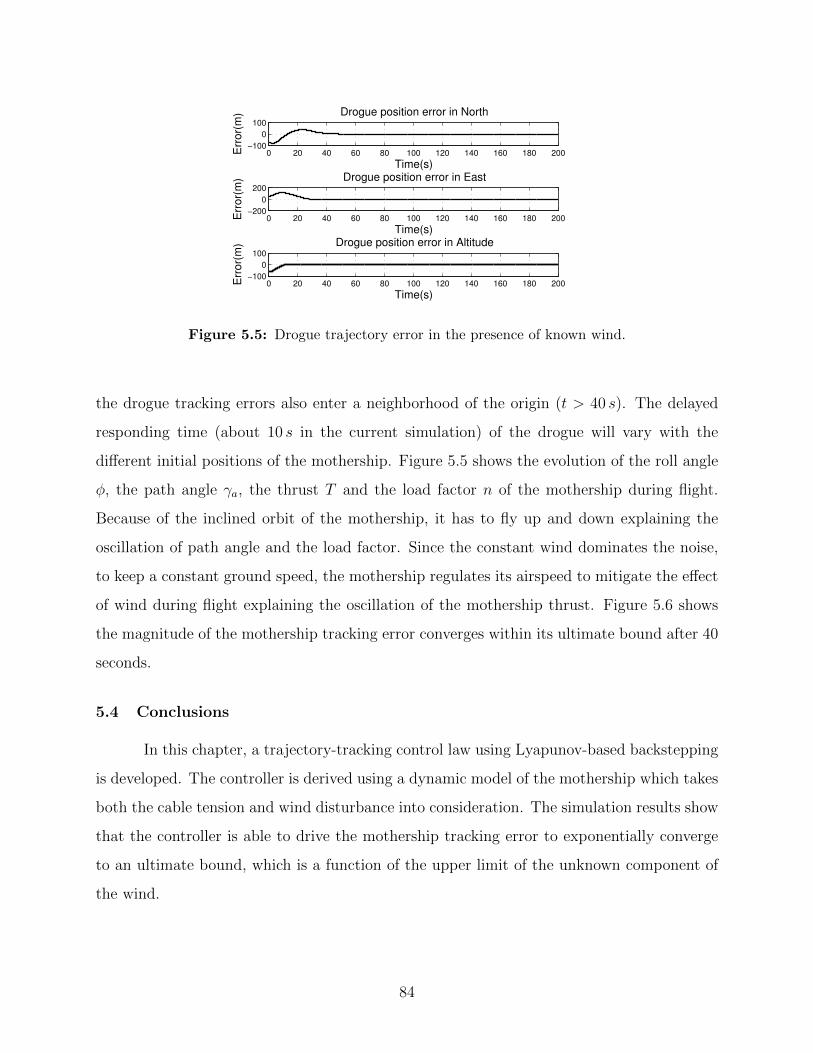
0 20 40 60 80 100 120 140 160 180 200−100
0
100
Drogue position error in North
Time(s)
Err
or(
m)
0 20 40 60 80 100 120 140 160 180 200−200
0
200
Drogue position error in East
Time(s)E
rro
r(m
)
0 20 40 60 80 100 120 140 160 180 200−100
0
100
Drogue position error in Altitude
Time(s)
Err
or(
m)
Figure 5.5: Drogue trajectory error in the presence of known wind.
the drogue tracking errors also enter a neighborhood of the origin (t > 40 s). The delayed
responding time (about 10 s in the current simulation) of the drogue will vary with the
different initial positions of the mothership. Figure 5.5 shows the evolution of the roll angle
φ, the path angle γa, the thrust T and the load factor n of the mothership during flight.
Because of the inclined orbit of the mothership, it has to fly up and down explaining the
oscillation of path angle and the load factor. Since the constant wind dominates the noise,
to keep a constant ground speed, the mothership regulates its airspeed to mitigate the effect
of wind during flight explaining the oscillation of the mothership thrust. Figure 5.6 shows
the magnitude of the mothership tracking error converges within its ultimate bound after 40
seconds.
5.4 Conclusions
In this chapter, a trajectory-tracking control law using Lyapunov-based backstepping
is developed. The controller is derived using a dynamic model of the mothership which takes
both the cable tension and wind disturbance into consideration. The simulation results show
that the controller is able to drive the mothership tracking error to exponentially converge
to an ultimate bound, which is a function of the upper limit of the unknown component of
the wind.
84

0 50 100 150 200−50
0
50
Time(s)φ (
de
g)
0 50 100 150 200−20
0
20
Time(s)
γ a (
de
g)
0 50 100 150 200−100
0
100
Time(s)
T (
N)
0 50 100 150 2000
1
2
Time(s)
n
Figure 5.6: Time evolution of the roll angle φ, path angle γa, thrust T and the load factor nof the mothership in the presence of wind.
0 20 40 60 80 100 120 140 160 180 2000
0.5
1
1.5
2
2.5
3
3.5
Time(s)
Err
or(
m)
Mothership error magnitude vs time
Mothership error
Ultimate bound
Figure 5.7: Time evolution of the magnitude of the tracking error of the mothership in thepresence of wind.
85

Chapter 6
Trajectory-Tracking Control Law Design for UAVs with Autopilotin the Loop
In the previous chapter, a nonlinear feedback control law was derived for the moth-
ership to follow the desired trajectory. However, the control inputs selected in the design
model are typically difficult to be directly applied in the experiment, because the autopilot
used to stabilize and control the vehicle, only accepts certain input commands. Strategies
dealing with this issue are not found in the literature.
In this chapter, we develop an approach of designing the trajectory tracking control
law for autonomous vehicles with the autopilot in the loop. The major contribution of this
chapter is that the specific interface structure of the autopilot is taken into account in the
controller design. To get the autopilot involved, the original designed trajectory tracking
controller and design model only need to be augmented using an extra term, which is the
function of the feedback error, so that the actual system trajectory is guaranteed to exponen-
tially converge to the reference trajectory with all states bounded. A sufficient condition for
qualified commands of the autopilot is also introduced. This strategy provide a framework
to implement the developed controller on the experimental vehicle with autopilot in the loop
without modifying the key structure of the design model and the original controller.
The remainder of the chapter is structured as follows. Section 6.1 introduces the
formulation of the problem. Section 6.2 develops the control strategy of trajectory-tracking
for UAVs with autopilot in the loop. Section 6.3 presents the numerical results using both
kinematic and dynamic models. Section 6.4 shows the results of software-in-the-loop simu-
lation.
86

Autopilot UAV Dynamics
Commands
Figure 6.1: Closed-loop control structure for UAVs. The autopilot performs the functions ofstabilizing the vehicle as well as following the specific commands.
Controller Design Model
Reference
Figure 6.2: Closed-loop control structure in trajectory tracking controller design.
6.1 Problem Formulation
This section formulates the trajectory tracking problem for UAVs with an autopilot
in the closed-loop system. A typical closed-loop structure of the feedback stabilization and
control in UAVs is shown in Fig. 6.0, where the autopilot performs the functions of stabilizing
the vehicle as well as following the input commands, which may include airspeed, altitude,
and attitude. A closed-loop structure of the feedback control for UAVs using a specific design
model is shown in Fig. 6.1, where the design model stands for the equations of motion of
UAVs (kinematic or dynamic models) and the controller is designed to achieve specific goals
(e.g. trajectory tracking or path following).
In particular, given the autopilot, the grey box shown in Fig. 6.2is fixed and cannot
be changed. Most commercial autopilots like Kestrel, Piccolo, etc., are black box systems,
in the sense that they implement specific autopilot functionality and we are constrained to
work with that functionality. However the input/output model of the autopilot/UAV system,
which is usually overly simplistic, may not be sufficient to capture the design requirements
for the control scheme (e.g., the case in aerial recovery). Therefore, it becomes desirable to
design a control strategy based on a medium fidelity model, and then to implement that
strategy on the autopilot.
87

Modified
ControllerModified
Design Model
Reference
Autopilot UAV Dynamics
Commands
Figure 6.3: Closed-loop control system in trajectory tracking with autopilot in the loop. Thecontroller and the design model are modified by feeding back the UAV states and sending thespecific commands that autopilot takes.
In this section, we are interested in the situation where the output of the controller
are not the same variables as the input commands for the autopilot. In order to use the con-
troller designed in Fig. 6.1 without any modifications to the autopilot, a closed-loop system
combining the systems shown in Figs. 6.0 and 6.1 is proposed as depicted in Fig. 6.2, where
the design model and controller are modified to drive the UAV position to exponentially
converge to and follow the reference. The main objective of this section is to develop a strat-
egy of augmenting the design model and the controller in Fig. 6.2 to achieve the trajectory
tracking for UAVs.
6.2 Trajectory-Tracking Control Law Design with Autopilot in the Loop
This section develops the control law of trajectory tracking for UAVs using the closed-
loop system in Fig. 6.2. Lyapunov based backstepping is employed to derive the controller
which is proved to be capable of driving the UAV to exponentially converge to and follow the
desired trajectory. The controller in Fig. 6.1 is firstly developed and the autopilot in Fig. 6.0
to follow the specific commands is developed after. An observer-based sufficient condition
is derived to examine the qualification of the commands that guarantees the convergence.
Finally, the augmentation law of the controller and design model is developed to complete
the theory.
6.2.1 Trajectory-Tracking Control Law Design Using Design Models
A trajectory tracking controller shown in Fig. 6.1 is developed in this section using a
specific design model .
88

Lemma 1: Defining the states η ∈ Dη ⊂ R3, ξ ∈ Dξ ⊂ R3 and the system inputs
u ∈ R3, consider the nonlinear system
˙η = f1
(ξ), (6.1)
˙ξ = f2
(ξ)
+ g2
(ξ)
u, (6.2)
where f1 : Dξ 7→ R3, f2 : Dξ 7→ R3, and g2 : Dξ 7→ R3 are smooth vector fields and locally
Lipschitz in ξ. Assuming that the Lie derivative [110] Lg2f1(ξ)
is invertible for ξ on Dξ,
and ηd(t) is C2 with bounded time-derivatives . If constants k1 and k2 are positive, and u is
selected as
u =(Lg2f1
(ξ))−1 (
ηd − Lf2f1(ξ)
−(k1 + k2
)(˙η − ηd
)−(
1 + k1k2
) (η − ηd
)), (6.3)
then the tracking error η− ηd converges exponentially to the origin and ξ remains bounded.
Proof:
Step 1: Convergence of η → ηd.
Let eη , η− ηd be the tracking error and the error dynamics is given by eη = ˙η− ηd.
Define the Lyapunov function candidate V1 = 12eTη eη, which has the time derivative
V1 = eTη eη
= eTη
(˙η − ηd
). (6.4)
At this stage of the development, we consider ˙η as a virtual control, where V1 can be made
negative definite by setting ˙η equals to ηd − k1eη. Introducing the error variable
z , ηd − k1eη − ˙η, (6.5)
and adding and subtracting z in (6.4) gives
V1 = −k1eTη eη − eTη z.
89

Consider the augmented Lyapunov function candidate
V2 , V1 +1
2zTz,
with the time derivative
V2 = −k1eTη eη + zT (−eη + z)
= −k1eTη eη + zT(−eη + ηd − k1eη − Lf2f1 − Lg2f1u
).
If u is given by (6.3), the time derivative of V2 becomes
V2 = −k1eTη eη − k2zTz. (6.6)
Based on Lyapunov stability theory [110], it can concluded that eη and z exponentially
converge to the origin.
Step 2: Boundedness of ξ.
From Eqs. (6.5) and (6.6) and the assumption that ηd is bounded, we have eη and z
are bounded, and then we have f1
(ξ)
is bounded. Since f1 is locally Lipschitz in ξ, we can
conclud that ξ is bounded.
6.2.2 Control Law Design for the Autopilot
A feedback control law for autopilot to follow the desired commands, shown in Fig. 6.0,
is developed in this section. The input commands are denoted as ξ in this section.
Lemma 2: Defining the states ξ ∈ Dξ ⊂ R3 and system inputs u ∈ R3, consider the
nonlinear system
ξ = f2 (ξ) + g2 (ξ) u,
90

Figure 6.4: Closed-loop control structure for trajectory tracking with autopilot in the loopusing generalized system dynamics. The commands sent to the autopilot are selected as y.
with the assumption that the function g2 (x) is invertible for x on Dξ. Suppose that ξ (t) ∈ Dξ
is C2 with bounded time-derivatives . If the constant k is positive, and u is selected as
u = g−12 (ξ)(−f2 (ξ) +
˙ξ − k
(ξ − ξ
)), (6.7)
then the tracking error ξ − ξ converges exponentially to the origin.
Proof:
Let eξ , ξ − ξ, then the error dynamic is given by eξ = ξ − ˙ξ. Define the Lyapunov
function candidate V3 = 12eTξ eξ, which has the time derivative
V3 = eTξ eξ
= eTξ
(f2 + g2u− ˙
ξ). (6.8)
If u is given by (6.7), the time derivative of V3 becomes
V3 = −keTξ eξ.
Based on Lyapunov stability theory, it can concluded that eξ exponentially converges to the
origin.
91

6.2.3 Sufficient Conditions for Qualified Commands of the Autopilot
The commands used in the previous subsection is selected as ξ. However, different
autopilots may accept different commands which may not always be ξ. In this section, we
propose an observer-based sufficient condition that can be used to examine whether the
commands of autopilot are qualified to guarantee that ξ → ξ.
Lemma 3: Suppose the commands that autopilot takes from the output of the design
model are y, which is a function of the system states x ,(ηT , ξT
)T, i.e., y , H (x) ∈ R3,
and the corresponding variables in the UAV dynamic are y , H (x) ∈ R3. Then y → y
implies that ξ → ξ, if the system (6.1) and (6.2) with output function y = H (x) is observable
with respect to ξ.
Proof:
If the system (6.1) and (6.2) with output function y = H (x) is observable respective
to ξ, it is implied that ξ can be reconstructed from y. Thus, if it is guaranteed that y → y,
it can be obtained that ξ → ξ.
6.2.4 Control Law Design Using Combined System
A control strategy, shown in Fig. 6.2, is presented in this section by augmenting the
design model and controller developed in Lemma 1. The UAV dynamics are selected as the
copy of the design model, and the autopilot control law is selected as the one developed in
Lemma 2. The combined systems using specific equations of motion are shown in Fig. 6.3.
The commands sent to the autopilot are selected as ξ.
Theorem 1: Defining the states η, η ∈ Dη ⊂ R3, ξ, ξ ∈ Dξ ⊂ R3, and the system
inputs u′, u ∈ R3, consider the nonlinear systems described in Fig. 6.3 with the assumption
that the Lie derivative Lg2f1 (x) is invertible for x on Dξ. Suppose that ηd(t) is C2 with
bounded time-derivatives . If constants k1, k2 and ` are positive, the extra term of the design
model is selected as
δ (t) = ` (η − η)
92

u is selected in (6.3), u is selected in ( 6.7), and the extra term of the developed controllerν (t)
is selected as
ν = −(Lg2f1
(ξ))−1 (
δ + k2δ), (6.9)
then the tracking error η − ηd and η − ηd converge exponentially to the origin and ξ and ξ
remain bounded for all t ≥ 0.
Proof:
The convergence of ξ to ξ follows from Lemma 2.
The convergence of η to η can be shown as follows.
Let eη , η − η and the error dynamic of eη is given by
˙eη = η − ˙η
= f1 (ξ)− f1(ξ)− `eη.
Because ξ exponentially converges to ξ, it can be concluded that f1 (ξ) exponentially con-
verges to f1
(ξ)
. Also, because ` is a positive constant, it can be concluded that the tracking
error eη exponentially converges to the origin since the linear system ˙eη = −`eη is input to
state stable [110].
The convergence of η → ηd can be shown as follow.
Let eη , η − ηd and the error dynamic of eη is given by eη = ˙η − ηd. Define the
Lyapunov function candidate V4 , 12eTη eη, which has the time derivative
V4 = eTη
(˙η − ηd
)= eTη
(f1
(ξ)
+ δ − ηd). (6.10)
Introducing the error variable
z , −f1(ξ)− δ + ηd − k1eη,
93

and adding and subtracting z in (6.10) gives
V4 = −k1eTη eη − eTη z.
Consider the augmented Lyapunov function candidate
V5 , V4 +1
2zT z,
with time derivative
V5 = −k1eTη eη + zT(−eη + ˙z
)= −k1eTη eη + zT
(−eη + ηd − k1eη
−δ − Lf2f1 − Lg2f1 (u + ν)).
If u is selected in (6.3) and ν is selected in (6.9), it can be obtained
V5 = −k1eTη eη − k2zT z.
Based on Lyapunov stability theorem [110] it can be concluded that eη exponentially con-
verges to the origin.
The boundedness of ξ and ξ can be shown as follow.
Because
z = −f1(ξ)− δ + ηd − k1eη,
and δ exponentially converges to the origin, it can be proved that ξ is bounded by using
the similar strategy in Lemma 1. From Lemma 2, it can be concluded that ξ exponentially
converges to ξ, so ξ is also bounded.
6.3 Numerical Results
In this section, simulation results are shown to validate the augmented controller
developed in the previous section. Both the kinematic and dynamic models are employed
to validate the controllers. The reference trajectory is selected as an inclined circular orbit.
94

Letting R be the desired orbit radius in the horizontal plane, Vd be the desired constant
ground speed, h0 be the desired average altitude and hc be the desired magnitude of the
altitude oscillation, the reference trajectory ηd in North-East-Down (NED) frame is given
by
ηd (t) =
R sin (ω0t)
R cos (ω0t)
−h0 + hc sin (ω0t)
, (6.11)
where ω0 = V dg /R. In this paper, R is selected as 200 m, Vd is selected as 14 m/s, h0 is
selected as 200 m and hc is selected as 10 m.
6.3.1 Simulation Results Using Kinematic Model
Letting (pn, pe, pd)T be the position of the UAV in NED frame, Va be the airspeed, ψ
be the heading angle, γa be the air mass referenced flight path angle, which is defined as the
angle from the inertial North-East plane to the velocity vector of the aircraft relative to the
air mass (wn, we, wd)T be the constant wind vector in NED frame, and airspeed rate uVa ,
heading angular rate uψ and flight path angular rate uγa be the control inputs, the equations
of motion of the UAV can be written as
pn = Va cosψ cos γa + wn, (6.12)
pe = Va sinψ cos γa + we, (6.13)
pd = −Va sin γa + wd, (6.14)
Va = uVa , (6.15)
ψ = uψ, (6.16)
γa = uγa . (6.17)
95

Table 6.1: Initial configuration of the system
Item UAV Dynamics Design Modelp0, m (0, 260, −180) (0, 220, −150)Va0, m/s 20 12ψ0, rad π
2π
γa0, rad 0 0φ0 rad 0 0
Comparing (6.12) to (6.17) with the equations in Fig. 6.3, it can be obtained that η =
(pn, pe, pd)T , ξ = (Va, ψ, γa)
T , u = (uVa , uψ, uγa)T , f2 (·) = 0, g2 (·) = I3 and
f1 (·) =
Va cosψ cos γa + wn
Va sinψ cos γa + we
−Va sin γa + wd
.
In the simulation, the control gains are selected as k = 2, k1 = 0.5, k2 = 2 and ` = 1. Letting
the initial position, airspeed, heading angle and flight path angle of the UAV be p0, Va0,
ψ0 and γa0, respectively, the initial configuration of the system in the simulation is listed in
Table 6.0. Without loss of generality The constant wind vector is selected as (3, 0, 0)T m/s.
The performance limits of the UAV are selected as ψ ∈ [−40, 40] deg/s, Va ∈ [10, 20] m/s,
γa ∈ [−15, 15] deg and φ ∈ [−35, 35] deg.
The simulation results are shown in Fig. 6.4. The UAV trajectories in the 3-D and
top-down views are shown in Fig. 6.4 (a) and (b), respectively. It can be seen that the actual
trajectory of the UAV started from a position outside the desired orbit with an initial distance
error approximately 60 m and converged to the desired trajectory after approximately a half
circle. Fig. 6.4 (c) shows the tracking error between the UAV trajectory and the reference
in North, East, and altitude directions. It can be seen that all the errors converged to zero
after 40 s. Fig. 6.4 (d) shows the evolution of the states Va, ψ and γa. The oscillation of Va is
due to the presence of wind and the oscillation of γa matched the desired altitude oscillation.
96

−200
0
200−200
0
200150
160
170
180
190
200
210
220
North, m
3−D view of system trajectory
East, m
Altitu
de
, m
Desired
Actual
(a) 3-D view of system trajectory.
−200 −100 0 100 200 300−250
−200
−150
−100
−50
0
50
100
150
200
250
Top−down view of system trajectory
East, m
No
rth
, m
DesiredActual
(b) Top-down view of system tra-jectory.
0 50 100 150−200
−100
0
100
UAS trajectory tracking error
No
rth
, m
0 50 100 150−200
0
200
400
Ea
st,
m
0 50 100 150−20
−10
0
10
t, s
Altitu
de
, m
(c) Trajectory tracking errors.
0 50 100 1500
10
20
30
Variable Evolutions
Va,
m/s
0 50 100 150−500
0
500
ψ,
de
g0 50 100 150
−10
0
10
20
γa,
de
g
t, s
(d) Evolution of the states.
Figure 6.5: Simulation results using kinematic model.
6.3.2 Simulation Results Using Dynamic Model
Although models that include kinematic relationships may be suitable for certain
control objectives, models that include dynamic effects are required for other purposes.
For example, the dynamics of the mothership used in the aerial recovery are affacted by
the tension force exerted from the cable. If this tension force cannot be neglected for the
mothership, the dynamic model needs to be utilized to design trajectory-tracking control
law fro the mothership.
Letting m be the UAV mass, g be the gravitational constant at Earth sea level, L
and D be the aerodynamic lift and drag forces, respectively, φ be the roll angle, the control
inputs be the thrust uτ , the load factor un , Lmg
and roll angular rate uφ, the dynamic model
97

of the UAV can be written as
pn = Va cosψ cos γa + wn, (6.18)
pe = Va sinψ cos γa + we, (6.19)
pd = −Va sin γa + wd, (6.20)
Va =uτ −Dm
− g sin γa, (6.21)
ψ =L sinφ
mVa cos γa, (6.22)
γa =g
Va(un cosφ− cos γa) , (6.23)
φ = uφ. (6.24)
To match the UAV dynamic model to 6.1 and 6.2, Equation (6.21) through (6.23) are rear-
ranged asVa
γa
ψ
=
−Dm− g sin γa
− gVa
cos γa
0
+
1m
0 0
0 gVa
cosφ 0
0 0 LmVa cos γa
uτ
un
µ
,
where µ , sinφ is the virtual control input. Then it can be obtained that
f2 (·) =
−Dm− g sin γa
− gVa
cos γa
0
, g2 (·) =
1m
0 0
0 gVa
cosφ 0
0 0 LmVa cos γa
,
u′ =
uτ
un
µ
.
Then the roll angular rate can be calculated by uφ =(sin−1 (u′ (3))− φ
)/Ts, where Ts is the
sample time of the simulation.
98

−200
0
200−200
−1000
100200
150
160
170
180
190
200
210
220
North, m
3−D view of system trajectory
East, m
Altitu
de
, m
Desired
Actual
(a) 3-D view of system trajectory.
−200 −100 0 100 200 300−250
−200
−150
−100
−50
0
50
100
150
200
250
Top−down view of system trajectory
East, m
No
rth
, m
DesiredActual
(b) Top-down view of system tra-jectory.
0 50 100 150−200
−100
0
100
UAS trajectory tracking error
No
rth
, m
0 50 100 150−200
0
200
400
Ea
st,
m
0 50 100 150−20
−10
0
10
t, s
Altitu
de
, m
(c) Trajectory tracking errors.
0 50 100 1500
10
20
30
Variable Evolutions
Va,
m/s
0 50 100 150−500
0
500
ψ,
de
g
0 50 100 150−10
0
10
20
γ a,
de
g0 50 100 150
−20
0
20
40
t, s
φ,
de
g
(d) Evolution of the states.
Figure 6.6: Simulation results using dynamic model.
In the simulation, the control gains are selected as k = 2, k1 = 0.2, k2 = 0.5, ` = 0.5.
Letting the initial roll angle be φ0, the initial configuration of the system in the simulation
is listed in Table 6.0. The constant wind vector is selected as (3, 0, 0)T m/s.
The simulation results are shown in Fig. 6.5 which was very similar to the results
using a kinematic model shown in Fig. 6.4. It can be seen that the convergence of the actual
trajectory was slightly slower than that in Fig. 6.4. The oscillation of the roll angle is due
to the presence of wind.
6.4 Software-In-the-Loop Simulation Results
In this section, a software-in-the-loop (SIL) simulation is conducted to validate the
control strategy developed in this chapter. The experimental platform consists of MATLAB,
MEX-function interface, Virtual Cockpit and a simulator, Aviones. The communication
structure is very similar to the one used in Chapter 3. For the current Kestrel Autopilot,
the commands that autopilot accepts are airspeed Va, course angle χ and the altitude −pd.
The course angle χ can be expressed as a function of heading angle ψ, air mass referenced
99

flight path angle γa and the wind estimation, which is given by [88]
χ = tan−1Va sinψ cos γa + weVa cosψ cos γa + wn
.
We can prove that the commands(Va, χ,−pd
)Tare qualified outputs that guarantee ξ → ξ
using Lemma 3 (See Appendix A).
The communication rate between MATLAB and VC is approximately 5 Hz, so the
step size in MATLAB is selected as 0.2 s. Because of the communication lag between the
MATLAB, Virtual Cockpit and the simulator, the control gain ` was tuned and selected as
0.1 to compromise between the tracking error of the actual and simulated UAV and tracking
error of the simulated UAV and the desired trajectory. A wind of 3 m/s from the west is
added in Aviones.
6.4.1 Circular Orbit Tracking
In this section, we use a circular orbit as a desired trajectory in the SIL simulation.
In Eq. (6.11), we select R as 200 m, V dg as 15 m/s, h0 as 100 m and hc as 5 m. A constant
wind (0, 3, 0) m/s is given in the simulator.
Figure 6.6 shows the SIL simulation results of tracking a circular orbit. Figure 6.6 (a)
presents the top-down view of system trajectories. It can bee seen that the actual trajectory
(line with “Asterisk”) started from approximately (−60,−40) and quickly converged to the
desired orbit (solid line). The UAV trajectory obtained from the design model (“diamond”
dots) also quickly converges to the desired orbit. Figure 6.6 (b) shows the side view of
system trajectories. It can be seen that the actual UAV altitude is able to essentially track
the desired orbit. Figure 6.6 (c) shows the tracking errors in the north, east and altitude
direction, respectively. It can be seen that tracking errors converge to the neighborhood
of the origin and oscillate within ±10 m in three directions, respectively. Figure 6.6 (d)
illustrates the distance between the actual UAV position and the desired trajectory. It
can be seen that the distance error converge to a small value (approximately 15 m) from a
large initial error (approximately 250 m) and remain within (15 m). Figure 6.6 (e) shows
the commanded autopilot inputs and the actual value of the UAV. It can be seen that the
100

−300 −200 −100 0 100 200 300−300
−200
−100
0
100
200
300
System Trajectories
East, m
Nort
h, m
ActualDesiredSimulated
(a) Top-down view of system trajectories.
−300 −200 −100 0 100 200 30080
85
90
95
100
105
110
115
120
System Trajectories
North, m
Altitude, m
Actual
Desired
Simulated
(b) Side view of system trajectories.
0 20 40 60 80 100 120 140 160−150
−100
−50
0
50
No
rth
, m
Tracking Errors
0 20 40 60 80 100 120 140 160−200
−100
0
Time, s
Ea
st,
m
0 20 40 60 80 100 120 140 160
−10
0
10
Time, s
Altitu
de
, m
(c) Tracking errors.
0 20 40 60 80 100 120 140 1600
50
100
150
200
250
Tracking Error in Distance
Time, s
Dis
tance, m
(d) Error in distance.
0 20 40 60 80 100 120 140 16090
100
110
H,
m
Autopilot Commands
Actual
Cmd
0 20 40 60 80 100 120 140 16010
15
20
Va,
m/s
0 20 40 60 80 100 120 140 160−5
0
5
Time, s
χ,
rad
(e) Commands and actual autopilot inputs.
0 20 40 60 80 100 120 140 160−1
−0.5
0
0.5
1
1.5
2
2.5
3
3.5
Time, s
Win
d s
pe
ed
, m
/s
Wind Estimation
Wn
We
(f) Wind estimation.
Figure 6.7: SIL simulation results in tracking a circular orbit.
altitude tracker has about 10 s lag. However, the airspeed and course angle trackers work
more precisely. Figure 6.6 (f) shows the wind estimation of VC. The wind estimation has
small offsets in both north and east directions. Besides the communication lag, the wind
estimation error is another key that results in large tracking errors.
101

6.4.2 Figure-8 Orbit Tracking
To further explore the effect of the control strategy, a figure-8 trajectory is employed
as the desired trajectory. Equations characterizing a typical figure-8 trajectory can be given
by
ηd (t) =
Ra sin (ϕ (t))
Rb sin (2 · ϕ (t))
−h0 + hc sin (ϕ (t))
.
To guarantee that the actual UAV is able to track the desired trajectory under its per-
formance limits, an updated law for ϕ is given to make sure the desired trajectory has a
constant airspeed in the presence of wind. The time derivative of ηd (t) can be calculated as
ηd =
Raϕ sinϕ
2Rbϕ cos (2ϕ)
hcϕ cosϕ
= va + w, (6.25)
where va is the airspeed vector in the wind frame. Thus, the airspeed magnitude of the UAV
Va = ‖va‖ is calculated as
Va =
√(Raϕ sinϕ− wn)2 + (2Rbϕ cos (2ϕ)− we)2 + (hcϕ cosϕ− wd)2.
Given a desired UAV airspeed V da , we can solving the quadratic equation for ϕ. In this
section, V da is selected as 14 m/s, Ra and Rb are selected as 250 m 100 m, respectively.
Figure 6.7 shows the SIL simulation results of tracking a figure-8 orbit. Figure 6.7 (a)
presents the top-down view of system trajectories. It can bee seen that the actual trajectory
(line with “Asterisk”) started from approximately (−80, 20) and is able to essentially follow
the desired orbit (solid line). The UAV trajectory obtained from the design model (“dia-
mond” dots) quickly converges to the desired orbit. Tracking errors of curved segments are
larger the straight part. Figure 6.7 (b) shows the side view of system trajectories. It can be
seen that the actual UAV altitude is able to essentially track the desired orbit. Figure 6.7 (c)
shows the tracking errors in the north, east and altitude direction, respectively. It can be
seen that tracking errors oscillate within ±50 m in the north and east directions, respectively,
102

−300 −200 −100 0 100 200 300−300
−200
−100
0
100
200
300
System Trajectories
East, m
Nort
h, m
Actual
Desired
Simulated
(a) Top-down view of system trajectories.
−300 −200 −100 0 100 200 30080
85
90
95
100
105
110
115
120
System Trajectories
North, m
Altitude, m
Actual
Desired
Simulated
(b) Side view of system trajectories.
0 50 100 150 200
−100
−50
0
50
No
rth
, m
Tracking Errors
0 50 100 150 200
0
50
100
Time, s
Ea
st,
m
0 50 100 150 200−5
0
5
Time, s
Altitu
de
, m
(c) Tracking errors.
0 50 100 150 2000
50
100
150
200
250
Tracking Error in Distance
Time, s
Dis
tance, m
(d) Error in distance.
0 50 100 150 20090
100
110
H,
m
Autopilot Commands
Actual
Cmd
0 50 100 150 20010
15
20
Va,
m/s
0 50 100 150 200−5
0
5
Time, s
χ,
rad
(e) Commands and actual autopilot inputs.
0 50 100 150 200−0.5
0
0.5
1
1.5
2
2.5
3
Time, s
Win
d s
pe
ed
, m
/s
Wind Estimation
Wn
We
(f) Wind estimation.
Figure 6.8: SIL simulation results in tracking a figure-8 orbit.
while ±5 m in the altitude direction. The figure-8 orbit is more complex than the circular
orbit with large curvature of the curved segment, which requires more maneuverability of
the vehicle. Figure 6.7 (d) illustrates the distance between the actual UAV position and
the desired trajectory. It can be seen that the distance error oscillates within ±50 m which
103

is much larger than that in Fig. 6.6 (d). Figure 6.7 (e) shows the commanded autopilot
inputs and the actual value of the UAV. It can be seen that the altitude tracker becomes
smaller than that in Fig. 6.6 (e), and the airspeed and course angle trackers work precisely.
Figure 6.7 (f) shows the wind estimation of VC. The wind estimation has small consistent
offsets in both north and east directions. It can be seen that, for more complex desired
trajectory, this control strategy needs high bandwidth. Onboard embedded implementation
could be an effective way.
6.5 Conclusions
This chapter presented a trajectory tracking strategy for UAVs with autopilot in
the closed-loop. Lyapunov based backstepping was used to derive the trajectory-tracking
controller using a design model with generalized equations of motion. To involve the autopilot
in the closed-loop system, the developed trajectory-tracking controller and the design model
were augmented. The updated controller was also proved using Lyapunov stability theory
to be capable of driving the vehicle to exponentially converge to and follow the reference
by keeping the other states bounded. The simulations using both kinematic and dynamic
models were conducted to validate the developed controllers. The numerical results showed
that the augmented controller was capable of achieving the trajectory-tracking objectives.
The SIL simulation results showed that this trajectory tracking control strategy is able
to drive the UAV to essentially track the desired circular and figure-8 trajectories. More
complex trajectories like figure-8 orbit requires higher communication bandwidth.
104

Chapter 7
Conclusions and Future Directions
7.1 Conclusions
In this dissertation, we focus on the strategy that places and stabilizes the path of an
aerial drogue, towed by a mothership aircraft using a long flexible cable, on a horizontally
flat orbit by maneuvering the mothership in the presence of wind. To achieve this goal,
several studies for towed cable systems are conducted, which include the dynamic modeling
for the cable, trajectory generation strategies for the mothership, trajectory-tracking control
law design, and simulation and flight test implementations. The main contributions and
results are summarized as follows.
In Chapter 2, a discretized approximation method based on finite element and lumped
mass is employed to model the cable dynamics. One contribution of this chapter is that two
approaches, Gauss’s Principle and Newton’s second law, are utilized to derive the equations
of motion for inelastic and elastic cables, respectively. For inelastic cables, Gauss’s Prin-
ciple provides a succinct method to model the system dynamics with complex kinematic
constraints by neglecting the internal forces. For elastic cables, Newton’s second law pro-
vides an effective and efficient method to formulate equations of motion for multi-link cable
dynamics with internal forces like cable tensions and external aerodynamic forces. Because
the cable using in the flight test is a fishing line, which expresses considerable stretch druing
the flight, The mathematical model for the cable-drogue system is derived using Newton’s
second law in the rest of the dissertation. The simulation results show the essential match to
the flight test results in both horizontal and vertical directions, respectively. The results also
illustrate that an increased number of cable links from 1 to 5 does not significantly improve
the accuracy of the predictions for the current configuration of the system.
105

In Chapter 3, differential flatness theory is employed to develop the trajectory gen-
eration approach for the mothership to place the drogue onto the desired orbit based on the
mathematical model developed in the previous chapter. One contribution of this chapter is
that different desired drogue orbits are utilized to generate the required mothership trajec-
tories in different wind conditions. The numerical results show that using the desired drogue
orbits with constant airspeed, the resulting mothership orbits present smaller altitude oscil-
lations and larger airspeed oscillations than using the drogue orbits with constant ground
speed. Another contribution of this chapter is that a wind update strategy is developed
which is capable of updating the precalculated required mothership orbit according to the
change of the wind estimation. The differential flatness based method has the advantages
like it is computationally inexpensive for discretized model of the cable, however, it requires
the system dynamic to be differentially flat and does not directly take performance limits of
the mothership into consideration. The flight test results show that the amplitude of drogue
altitude oscillation can be stabled within 10 m in the presence of wind of approximately
4 m/s. The tracking error of the drogue may result from several reasons like the inaccuracy
of the model, imprecise and delayed wind estimation, wind gust and the tracking error of
the mothership.
In Chapter 4, model predictive control (MPC) is utilized to develop the trajectory
generation approach for the mothership to lead the drogue onto the desired orbit. The MPC
method is based on optimization theory which can be applied to most dynamical systems and
is able to take the performance limits of the mothership into consideration. One contribution
of this chapter is that a combination objective function is developed in which a squared-error
objective is used to calculate the trajectory tracking error and L1-norm objectives are used
to regulate the constraints. Different desired drogue trajectories are also used to produce
the required mothership trajectories in different wind conditions. The numerical results
show that even in severe wind conditions (e.g. wind speed greater than 10 m/s), the MPC
based method is able to produce trajectories that guarantee that the mothership maneuvers
within its performance limits as well as placing the drogue essentially onto the desired orbit.
Trajectory generation for a transitional flight in which the system flies from a straight and
level flight into a circular orbit, is also presented. The cable tension is added as an additional
106

constraint so that the tension force variates within its limits during the transition. Primary
drawbacks of the optimization based method include that it is computationally expensive
and that it is difficult to configure relative to the method based on differential flatness. The
possibility of an unsuccessful solution may also limit this method from being applied in the
real time. This MPC-based optimal trajectory generation strategy can be a framework for
specifying any arbitrary flight path of the towed body by optimizing the action of the towing
vehicle subject to constraints and wind disturbance.
In Chapter 5, a trajectory tracking control law for the mothership is developed using
Lyapunov based backstepping in the presence of wind. One contribution of this chapter
is that the cable tension and wind disturbance are taken into account in the mothership
dynamics and the mothership tracking error is guaranteed to exponentially converge to an
ultimate bound, which is a function of a superior limit of the unknown component of the
wind.
In Chapter 6, we develop an approach of designing the trajectory tracking control law
for autonomous vehicles with the autopilot in the loop. One contribution of this chapter is
that the specific dynamic of the autopilot is taken into account in the controller design. The
original designed trajectory tracking controller and design model only need to be augmented
using an extra term which is a function of the feedback error, so that the actual system
trajectory is guaranteed to exponentially converge to the origin with all states bounded. A
sufficient condition for qualified commands of the autopilot is also developed. This strategy
provide a framework to implement the developed controller on the experimental vehicle
without modifying the key structure of the design model and the controller.
7.2 Future Directions
A number of potential topics may be explored in the future work based on the contri-
butions and results of this dissertation. In this section, we propose several possible directions.
Two methods are employed in Chapter 2, to derive the equations of motion for the
cable dynamics. The flight test data are used to determine an appropriate number of cable
links. However, it is nontrivial to determine reasonable values for key parameters like drag
coefficient of the drogue, cable length, and Young’s modulus. Therefore, an estimation based
107

strategy is needed that utilizes the experimental data to determine values for parameters in
the simulation .
Existing methods that solve the motion planning problem for towed cable systems
are typically based on optimization and differential flatness, as discussed in Chapter 3 and 4.
However, these two methods are primarily used in offline calculations. Because the differen-
tial flatness based method does not take the performance limits and constraints like cable
tension into consideration, for realtime application, it may not be suitable to produce required
trajectories for towing vehicles with low maneuverability. The optimization based method
has drawbacks like computationally expensive and possibly infeasible solutions, which may
be impractical in real-time application. Therefore, a real-time trajectory generation strategy
for towed cable systems is needed.
In this dissertation, the trajectory tracking objective for the drogue is achieved by
assuming that the drogue motion is able to follow the desired trajectory if the mothership
tracks the required trajectory. This is actually an open-loop control strategy. The traditional
closed-loop control strategy is hard to apply to the towed cable system because the cable
connection between the mothership and drogue delays the drogue response to the mothership
maneuvering. However, periodic feedback control may be a potential approach that is able to
solve the problem. One possible way is to linearize the system dynamics around the desired
drogue trajectory. A periodic update strategy for the mothership motion is also needed by
feeding back the target control variables of the drogue (e.g. the oscillation of the drogue
altitude).
In Chapter 3, the experimental results show that the mothership is able to essen-
tially follow the calculated trajectory in the flight test using waypoint following. The current
experimental platform that implements developed control law in the flight test consists of
MATLAB, MEX-function interface, Virtual Cockpit and the autopilot. The developed con-
troller is implemented in MATLAB to compute the control inputs using the telemetry data.
MEX-function interface is used to transfer the telemetry data and the control inputs between
Virtual Cockpit and MATLAB. Virtual Cockpit is employed to control the airplane by send-
ing the commands to the autopilot. However, the current communication frequency between
MATLAB and Virtual Cockpit is approximately 5 Hz, and the commands that Virtual Cock-
108

pit accepts are typically variables like altitude, course angle and airspeed. The course angle
and altitude following in the autopilot belong to the outer loop control with low bandwidth
so that the maneuverability of the vehicle is attenuated. Therefore, the accessibility to inner
loop controlled variables like bank angle and pitch angle are needed. It is also required that
the communication frequency between MATLAB and Virtual Cockpit increase to at least
25 Hz, which is the communicate rate between the Virtual Cockpit and the autopilot.
109

Bibliography
[1] R. A. Skop and Y. Choo, “The configuration of a cable towed in a circular path,”Journal of Aircraft, vol. 8, no. 11, pp. 856–862, November 1971. 2, 6, 7, 9
[2] R. Murray, “Trajectory generation for a towed cable system using differential flatness,”13th Triennial World Congress of the International Federation of Automatic Control,pp. 395–400, 1996. 2, 10, 12, 13, 19, 24, 38, 56, 81
[3] P. Williams and P. Trivailo, “Dynamics of circularly towed cable systems, part 1:Optimal configurations and their stability,” AIAA Journal of Guidance, Control, andDynamics, vol. 30, no. 3, pp. 753–765, May-June 2007. 2, 8, 9, 10, 25, 26, 27, 38, 54
[4] ——, “Dynamics of circularly towed cable systems, part 2: Transitional flight anddeployment control,” AIAA Journal of Guidance, Control, and Dynamics, vol. 30,no. 3, pp. 766–779, May-June 2007. 2, 9, 12, 54, 67
[5] T. Wyllie, “Parachute recovery for UAV systems,” Aircraft Engineering and AerospaceTechnology, vol. 73, no. 6, pp. 542–551, 2001. 4
[6] K. Mullens, A. Burmeister, M. Wills, N. Stroumtsos, T. Denewiler, K. Thomas, andS. Stancliff, “Automated launch, recovery, and refueling for small Unmanned AerialVehicles,” Mobile Robots XVII, Society of Photo-Optical Instrumentation Engineers,SPIE Proceedings Series, vol. 5609, pp. 233–243, 2004. 4
[7] G. Avanzini and G. de Matteis, “Design of a shipboard recovery system for a shrouded-fan UAV,” no. 563. Toronto, Canada: Proceedings of 23rd ICAS Congress, September2002. 5
[8] S. Khantsis and A. Bourmistrova, “Stochastic design of a non-linear controller forautonomous UAV recovery.” Proceeding of International Congress on Modelling andSimulation, 2005, pp. 1258–1264. 5
[9] F. Wong, E. Gagnon, K. McTaggart, J. Colwell, S. Zan, and O. Theriault, “A paramet-ric study of factors affecting successful ship recovery of UAVs,” Defence R&D Canada,Valcartier, Tech. Rep., 2008. 5
[10] A. D. Kahn, “Vision-based recovery and guidance for small unmanned air vehicles,”in AIAA Guidance, Navigation, and Control Conference, Toronto, Ontario Canada,August 2010. 5
[11] M. A. Watts, J. George Raymond Root, and D. M. Adamski, “UAV recovery system,”U.S. Patent 7 219 856B2, 2007. 5, 6
110

[12] J. Snediker, M. A. Watts, and G. W. Corboy, “UAV arresting hook for use with UAVrecovery system,” U.S. Patent 7 143 976B2, 2006. 6
[13] J. Snediker, “UAV recovery system II,” U.S. Patent 7 510 145B2, 2009. 6
[14] L. Sun, R. W. Beard, M. B. Colton, and T. W. McLain., “Dynamics and control ofcable-drogue system in aerial recovery of micro air vehicles based on Gauss’s principle,”in American Control Conference, St. Louis, MO, USA, June 2009, pp. 4729–4734. 6,9, 12, 24
[15] L. Sun, R. W. Beard, and M. B. Colton, “Motion planning and control for mothership-cable-drogue systems in aerial recovery of micro air vehicles,” in American ControlConference, Baltimore, MD, USA, 2010, pp. 2101 – 2106. 6, 9, 12, 38, 56
[16] L. Sun and R. W. Beard, “Towed body altitude stabilization and states estimationin aerial recovery of micro air vehicles,” in AIAA Guidance, Navigation, and ControlConference, Toronto, Ontario Canada, August 2010. 8, 11, 12, 25, 74
[17] D. C. Carlson and M. B. Colton, “Out-of-plane orbit estimation and tracking for aerialrecovery of micro air vehicles,” in 2010 IEEE International Conference on Robotics andAutomation, Anchorage, Alaska, USA, 2010.
[18] L. Sun and R. W. Beard, “Towed-body trajectory tracking in aerial recovery of microair vehicle in the presence of wind,” in American Control Conference, San Francisco,CA, USA, 2011, pp. 3209–3214. 9, 12, 38, 56
[19] M. B. Colton, L. Sun, D. C. Carlson, and R. W. Beard, “Multi-vehicle dynamics andcontrol for aerial recovery of micro air vehicles,” Int. J. Vehicle Autonomous Systems,vol. 9, pp. 78–107, 2011. 8, 38
[20] M. A. Owen, J. W. Nichols, and M. B. Colton, “Cooperative aerial tracking andrendezvous along time-optimal 3-dimensional curves,” in AIAA Guidance, Navigation,and Control Conference, Portland, OR, USA, August 2011.
[21] J. Nichols, J. Ferrin, M. Owen, and T. McLain, “Vision-enhanced aerial rendezvousalong elliptical paths,” in AIAA Guidance, Navigation, and Control Conference, Min-neapolis, MN, USA, August 2012.
[22] J. Ferrin, J. Nichols, and T. McLain, “Design and control of a maneuverable towedaerial vehicle,” in AIAA Guidance, Navigation, and Control Conference, Minneapolis,MN, USA, August 2012.
[23] J. Nichols and L. Sun, “Autonomous aerial rendezvous of small unmanned aircraftsystems using a towed cable system,” in 43rd Annual Society of Flight Test EngineersSymposium, Fort Walton Beach, FL, USA, October 2012. 6
[24] F. M. Wilson-Jr. and A. G. Bennett, “New concept for low cost VTOL cargo deliverycapability,” AIAA Meeting Paper Archive Set, vol. 244, pp. 324–335, 1983. 6
111

[25] J. O’Donnell, “Air pick up,” EnRoute, vol. 9, no. 1, 2000.
[26] P. Trivailo, D. Sgarioto, and C. Blanksby, “Optimal control of aerial tethers for payloadrendezvous,” in Proceedings of the 5th Asian Control Conference, 2004, pp. 396–404.12
[27] P. Williams and P. Trivailo, “Cable-supported sliding payload deployment from a cir-cling fixed-wing aircraft,” Journal of Aircraft, vol. 43, no. 5, pp. 1567–1569, 2006.
[28] P. Williams and W. Ockels, “Dynamics of towed payload system using multiple fixed-wing aircraft,” AIAA Journal of Guidance, Control, and Dynamics, vol. 32, no. 6, pp.1766–1780, November-Decemeber 2009. 6, 9
[29] T. S. Walton and H. Polachek, “Calculation of transient motion of submerged cables,”Mathematics of Computation, vol. 14, pp. 27–46, 1960. 6
[30] S. Jones and J. Krausman, “Nonlinear dynamic simulation of a tethered aerostat,”Journal of Aircraft, vol. 19, no. 8, pp. 679–686, 1982. 9
[31] C. Lambert and M. Nahon, “Stability analysis of a tethered aerostat,” Journal ofAircraft, vol. 40, no. 4, pp. 705–715, 2003. 8, 10
[32] P. Williams, B. Lansdorp, and W. Ockels, “Optimal cross-wind towing and powergeneration with tethered kites,” AIAA Journal of Guidance, Control, and Dynamics,vol. 31, no. 1, pp. 81–93, 2008. 6, 9, 19
[33] F. S. Hover, “Experiments in dynamic positioning of a towed pipe,” in OCEANS ’93.Engineering in Harmony with Ocean, vol. 3, Victoria, BC , Canada, Oct 1993, pp.III484 – III490. 6, 11, 12, 13
[34] R. G. Borst, G. F. Greisz, and A. G. Quynn, “Fuzzy logic control algorithm for sup-pressing E-6A long trailing wire antenna wind shear induced oscillations,” in AIAAGuidance, Navigation, and Control Conference, August 1993. 9, 11, 12
[35] A. S. Bourmistrov, R. D. Hill, and P. Riseborough, “Nonlinear control law for aerialtowed target,” AIAA Journal of Guidance, Control, and Dynamics, vol. 18, no. 6, pp.1232–1238, 1995. 12, 24
[36] J. M. Clifton, L. V. Schmidt, and T. D. Stuart, “Dynamic modeling of a trailing wiretowed by an orbiting aircraft,” AIAA Journal of Guidance, Control, and Dynamics,vol. 18, no. 4, pp. 875–881, 1995. 9, 11, 24
[37] D. L. Brushwood, A. P. Olsont, and J. M. Smyth, “The E-6A orbit improvementsystem and its effect upon LTWA verticality,” 1998. 12
[38] J. F. Henderson, J. Potjewyd, and B. Ireland, “The dynamics of an airborne towedtarget system with active control,” in Proceedings of the Institution of MechanicalEngineers, Part G: Journal of Aerospace Engineering, 1999. 9, 10, 12
112

[39] J. W. Kamman and R. L. Huston, “Modeling of variable length towed and tetheredcable systems,” AIAA Journal of Guidance, Control, and Dynamics, vol. 22, no. 4, pp.602–608, 1999. 10
[40] S. Yamaguchi, W. Koterayama, and T. Yokobiki, “Development of a motion controlmethod for a towed vehicle with a long cable,” in Proceedings of the 2000 InternationalSymposium on Underwater Technology, Tokyo , Japan, May 2000, pp. 491 – 496. 9,10, 12, 13
[41] Y. Turkyilmaz and O. Egeland, “Active depth control of towed cables in 2D,” IEEEConference on Decision and Control, pp. 952–957, December 2001. 9, 12
[42] M. Vannahme and G. F. Clauss, “Non-linear dynamics of vertically tethered and towedbody systems,” no. 133. Crete, Hellas: Proc. of the 10th Int. Congress of the Int.Maritime Assoc. of the Mediterranean (IMAM), 2002.
[43] T. Nguyen and O. Egeland, “Stabilization of towed cables,” in 43rd IEEE Conferenceon Decision and Control, vol. 5, December 2004, pp. 5059–5064. 9
[44] T. L. Richardson, “Parametric study of the towline shape of an aircraft decoy,” Mas-ter’s thesis, Air Force Institute of Technology, 2005.
[45] P. Williams and P. Trivailo, “Stability and equilibrium of a circularly-towed aerialcable system with an attached wind-sock,” in AIAA Atmospheric Flight MechanicsConference and Exhibit, San Francisco, CA, August 2005, pp. 1–33. 6, 8, 9
[46] G. Frost and M. Costello, “Improved deployment characteristics of a tether-connectedmunition system,” AIAA Journal of Guidance, Control, and Dynamics, vol. 24, no. 3,pp. 547–554, 2001. 6, 9, 10
[47] S. R. Norris and D. I. Andrisani, “Longitudinal equilibrium solutions for a towedaircraft and tow cable,” in AIAA paper 2001-4254, 2001. 6, 9
[48] P. Williams, “Optimal terrain-following for towed-aerial-cable sensors,” Multibody SystDyn, vol. 16, pp. 351–374, 2006. 6, 9, 12, 38
[49] K. Ro and J. W. Kamman, “Modeling and simulation of [Hose-Paradrogue aerial refu-eling systems,” AIAA Journal of Guidance, Control, and Dynamics, vol. 33, pp. 53–63,2010. 6
[50] D. E. Sgarioto, “Non-linear dynamic modelling and optimal control of aerial tethersfor remote delivery and capture of payloads,” Ph.D. dissertation, School of AerospaceMechanical and Manufacturing Engineering, RMIT University, June 2006. 6, 38
[51] I. Kolodner, “Heavy rotating string – a nonlinear eigenvalue problem,” Communica-tions on Pure and Applied Mathematics, vol. 8, pp. 395–408, 1955. 7, 9
[52] B. J. Barnes and J. L. Pothier, “Wind tunnel measurement of airborne towed cabledrag coefficient,” Master’s thesis, Air Force Institute of Technology, 1971. 7
113

[53] C. Wu, “Whirling of a string at large angular speeds – a nonlinear eigenvalue problemwith moving boundary layers,” SIAM J. on Applied Mathematics, vol. 22, no. 1, pp.1–13, 1972. 7, 9
[54] J. J. Russell and W. J. Anderson, “Equilibrium and stability of a whirling rod-masssystem,” Int. J. Non-Linear Mechanics, vol. 12, pp. 91–101, 1977. 7
[55] ——, “Equilibrium and stability of a circularlytowed cable subject to aerodynamicdrag,” Journal of Aircraft, vol. 14, no. 7, pp. 680–686, 1977. 7, 9
[56] N. Nakagawa and A. Obata, “Longitudinal stability analysis of aerial-towed systems,”Journal of Aircraft, vol. 29, no. 6, pp. 978–985, 1992. 7, 9
[57] B. Etkin, “Stability of a towed body,” Journal of Aircraft, vol. 35, no. 2, pp. 197–205,1998. 7, 9, 10
[58] P. Williams and P. Trivaio, “Periodic solutions for flexible cable-body systems towedin circular and elliptical paths,” in AIAA Atmospheric Flight Mechanics Conferenceand Exhibit, Keystone, Colorado, August 2006. 8, 9
[59] L. Sun, J. D. Hedengren, and R. W. Beard, “Optimal trajectory generation usingmodel predictive control for aerially towed cable systems (to appear),” AIAA Journalof Guidance, Control, and Dynamics, 2013. 8, 11, 12, 13
[60] T. K. Caughey, “Whirling of a heavy chain,” in Third U. S. National Congress ofApplied Mechanics, June 1958, pp. 101–108. 9
[61] J. Genin, S. J. Citron, and R. R. Huffman, “Coupling of longitudinal and transversemotions of a flexible cable in a uniform flow field,” The Journal of the AcousticalSociety of America, vol. 52, no. 1B, pp. 438–440, 1972. 9
[62] C. Chin, R. May, and H. Connell, “A numerical model of a towed cable-body system,”ANZIAM Journal, vol. 42, pp. C362–C384, 2000. 10
[63] J. Coomer, M. Lazarus, R. Tucker, D. Kershaw, and A. Tegman, “A non-linear eigen-value problem associated with inextensible whirling strings,” Journal of Sound andVibration, vol. 239, pp. 969–982, 2001.
[64] G. Lemon and W. B. Fraser, “Steady-state bifurcations and dynamical stability ofa heavy whirling cable acted on by aerodynamic drag,” in Royal Society of LondonProceedings Series A, vol. 457, 2001, pp. 1021–1041. 9
[65] J. E. J. Cochran, M. Innocenti, T. S. No, and A. Thukral, “Dynamics and controlof maneuverable towed flight vehicles,” AIAA Journal of Guidance, Control, and Dy-namics, vol. 15, no. 5, pp. 1245–1252, 1992. 9, 11, 12, 24, 26, 27
[66] J. E. Quisenberry, “Dynamic simulation of low altitude aerial tow systems,” Master’sthesis, Oklahoma State University, Stillwater, Oklahoma, 2002.
114

[67] J. E. Quisenberry and A. S. Arena, “Dynamic simulation of low altitude aerial towsystems,” in AIAA Atmospheric Flight Mechanics Conference and Exhibit, vol. 1, Prov-idence, Rhode Island, August 2004, pp. 243–252. 24
[68] P. Williams, D. Sgarioto, and P. Trivai, “Motion planning for an aerial-towed cablesystem,” in AIAA Guidance, Navigation, and Control Conference, August 2005. 12,13, 38, 56
[69] P. Williams, “Periodic optimal control of a towed aerial-cable system in presence ofcross-wind,” in AIAA Guidance, Navigation, and Control Conference, Keystone, Col-orado, August 2006. 13, 19, 38, 54
[70] P. Williams, D. Sgarioto, and P. Trivailo, “Optimal control of an aircraft-towed flexiblecable system,” AIAA Journal of Guidance, Control, and Dynamics, vol. 29, no. 2, pp.401–410, March–April 2006. 13, 38
[71] P. Williams, D. Sgarioto, and P. M. Trivailo, “Constrained path-planning for an aerial-towed cable system,” Aerospace Science and Technology, vol. 12, pp. 347–354, 2008.54
[72] P. Williams, “Optimization of circularly towed cable system in crosswind,” AIAAJournal of Guidance, Control, and Dynamics, vol. 33, no. 4, pp. 1251–1263, July-August 2010. 9, 38, 54, 64
[73] P. Williams, P. Lapthorne, and P. Trivailo, “Circularly-towed lumped mass cable modelvalidation from experimental data,” in AIAA Modeling and Simulation TechnologiesConference and Exhibit, Keystone, Colorado, August 2006. 9, 11, 19
[74] Y. Choo and M. J. Casarella, “A survey of analytical methods for dynamic simulationof cable-body systems,” Journal of Hydronautics, vol. 7, no. 4, pp. 137–144, 1973. 9,10, 19
[75] F. Zhu and C. D. Rahn, “Stability analysis of a circularly towed cable-body system,”Journal of Sound and Vibration, vol. 217, no. 3, pp. 435–452, May 1998. 10
[76] T. Dreyera and J. H. V. Vuuren, “A comparison between continuous and discretemodelling of cables with bending stiffness,” Applied Mathematical Modelling, vol. 23,pp. 527–541, 1999. 10
[77] M. Fliess, J. Levine, P. Martin, and P. Rouchon, “Flatness and defect of non-linearsystems: introductory theory and examples,” International Journal of Control, vol. 61,no. 6, pp. 1327–1361, 1995. 13, 38, 40, 54
[78] P. Aguiar, D. Dacic, J. Hespanha, and P. Kokotivic, “Path-following or reference-tracking? An answer relaxing the limits to performance,” in IAV2004, 5thIFAC/EURON Symposium on Intelligent Autonomous Vehicles, Lisbon, Portugal,2004. 14
115

[79] A. Micaelli and C. Samson, “Trajectory tracking for unicycle-type and two-steering-wheels mobile robots,” The French National Institute for Research in Computer Scienceand Control, Sophia-Antipolis, France, Technical Report 2097, 1993. 14
[80] I. Kolmanovsky and N. H. McClamroch, “Developments in nonholonomic control prob-lems,” IEEE Control Systems, vol. 15, no. 6, pp. 20–36, Dec. 1995. 14
[81] A. W. Divelbiss and J. T. Wen, “Trajectory tracking control of a car-trailer system,”IEEE Transactions on Control Systems Technology, vol. 5, no. 3, pp. 269–278, May1997. 14
[82] I. Kaminer, A. Pascoal, E. Hallberg, and C. Silvestre, “Trajectory tracking for au-tonomous vehicles: An integrated approach to guidance and control,” AIAA Journalof Guidance, Control, and Dynamics, vol. 21, no. 1, pp. 29–38, 1998. 14
[83] P. Encarnacao and A. Pascoal, “Combined trajectory tracking and path following formarine craft.” Orlando, FL: the IEEE Conference on Decision and Control, 2001, pp.964–969. 14
[84] A. P. Aguiar, L. Cremean, and J. P. Hespanha, “Position tracking for a nonlinearunderactuated hovercraft: controller design and experimental results,” in Proc. 42ndIEEE Conference on Decision and Control, vol. 4, 9–12 Dec. 2003, pp. 3858–3863. 14
[85] A. P. Aguiar and J. P. Hespanha, “Position tracking of underactuated vehicles,” inProc. American Control Conference the 2003, vol. 3, 4–6 June 2003, pp. 1988–1993.14
[86] ——, “Trajectory-tracking and path-following of underactuated autonomous vehicleswith parametric modeling uncertainty,” IEEE Transactions on Automatic Control,vol. 52, no. 8, pp. 1362–1379, August 2007. 15, 74
[87] D. R. Nelson, D. B. Barber, T. W. McLain, and R. W. Beard, “Vector field pathfollowing for miniature air vehicles,” IEEE Transactions on Robotics, vol. 37, pp. 519–529, June 2007. 15
[88] R. W. Beard and T. W. McLain, Small Unmanned Aircraft: Theory and Practice.Princeton University Press, 2012. 15, 51, 57, 100
[89] H. Chao, Y. Cao, and Y. Chen, “Autopilots for small fixed-wing unmanned air vehicles:A survey,” in Proceedings of the 2007 IEEE International Conference on Mechatronicsand Automation, Harbin, China, August 2007. 15
[90] I. Kaminer, A. Pascoal, E. Xargay, N. Hovakimyan, C. Cao, and V. Dobrokhodov,“Path following for unmanned aerial vehicles using l1adaptive augmentation of com-mercial autopilots,” AIAA Journal of Guidance, Control, and Dynamics, vol. 33, no. 2,pp. 550–564, 2010. 15
116

[91] V. Dobrokhodov, I. Kaminer, I. Kitsios, E. Xargay, N. Hovakimyan, C. Cao, I. M.Gregory, and L. Valavani, “Experimental validation of L1 adaptive control: The rohrscounterexample in flight,” AIAA Journal of Guidance, Control, and Dynamics, vol. 34,no. 5, pp. 1311–1328, 2011. 15
[92] F. E. Udwadia and R. E. Kalaba, Analytical Dynamics: A New Approach. Cambridge,New York: Cambridge University Press, 1996. 19, 20, 21
[93] T. W. McLain and R. W. Beard, “Trajectory planning for coordinated rendezvous ofunmanned air vehicles,” vol. 4369, pp. 1–8, 2000. 19, 24
[94] S. Qin and T. Badgwell, “An overview of industrial model predictive control technol-ogy,” in Proc. CPC V, 1997, pp. 232–256. 55
[95] ——, Nonlinear Model Predictive Control. Boston, MA: Birkhauser Verlag, 2000, ch.An overview of nonlinear model predictive control applications, pp. 369–392.
[96] ——, “A survey of industrial model predictive control technology,” Control EngineeringPractice, vol. 11, pp. 733–764, 2003. 55
[97] R. Findeisen, F. Allgower, and L. Biegler, Assessment and future directions of nonlin-ear model predictive control. Berlin: Springer-Verlag, 2007. 55
[98] T. Binder, L. Blank, H. Bock, R. Burlisch, W. Dahmen, M. Diehl, T. Kronseder,W. Marquardt, J. Schloder, and O. Stryk, Online Optimization of Large Scale Systems.Springer-Verlag Berlin Heidelberg, 2001, ch. Introduction to model based optimizationof chemical processes on moving horizons, pp. 295–339. 55
[99] J. Albuquerque and L. Biegler, “Decomposition algorithms for on-line estimation withnonlinear DAE models,” Computers and Chemical Engineering, vol. 21, no. 3, pp.283–299, 1997. 55
[100] M. Diehl, H. G. Bock, J. P. Schloder, R. Findeisen, Z. Nagy, , and F. Allgower,“Real-time optimization and nonlinear model predictive control of processes governedby differential-algebraic equations,” Journal of Process Control, vol. 12, pp. 577–585,2002. 55
[101] A. Wachter and L. Biegler, “On the implementation of a primal-dual interior pointfilter line search algorithm for large-scale nonlinear programming,” Mathematical Pro-gramming, vol. 106, no. 1, pp. 25–57, 2006. 55
[102] E. Haseltine and J. Rawlings, “Critical evaluation of extended kalman filtering andmoving-horizon estimation,” Ind. Eng. Chem. Res., vol. 44, no. 8, pp. 2451–2460,2005. 55
[103] B. Odelson, M. Rajamani, and J. Rawlings, “A new autocovariance least-squaresmethod for estimating noise covariances,” Automatica, vol. 42, no. 2, pp. 303–308,February 2006.
117

[104] J. Hedengren and T. Edgar, “Moving horizon estimation - the explicit solution,” inProceedings of Chemical Process Control (CPC) VII Conference, Lake Louise, Alberta,Canada, 2006.
[105] B. Spivey, J. Hedengren, and T. Edgar, “Monitoring of process fouling using first-principles modeling and moving horizon estimation,” in Proc. Texas, Wisconsin, Cal-ifornia Control Consortium (TWCCC), Austin, TX, 2009. 55
[106] J. Hedengren, K. Allsford, and J. Ramlal, “Moving horizon estimation and controlfor an industrial gas phase polymerization reactor,” in Proceedings of the AmericanControl Conference (ACC), New York, NY, 2007, pp. 1353–1358. 55
[107] M. Darby, M. Nikolaou, J. Jones, and D. Nicholson, “RTO: An overview and assessmentof current practice,” Journal of Process Control, vol. 21, pp. 874–884, 2011. 55
[108] J. Hedengren, “APMonitor Modeling Language,” apmonitor.com, Dec 2011. 56, 60
[109] A. Wachter and L. T. Biegler, “On the implementation of a primal-dual interior pointfilter line search algorithm for large-scale nonlinear programming,” Mathematical Pro-gramming, vol. 106, no. 1, pp. 25–57, 2006. 61
[110] H. K. Khalil, Nonlinear Systems, 3rd ed. Upper Saddle River, NJ: Prentice Hall,2002. 74, 80, 89, 90, 93, 94
[111] R. Skjetne, T. Fossen, and P. Kokotovic, “Robust output maneuvering for a class ofnonlinear systems,” Automatica, vol. 40, no. 3, pp. 373–383, 2004. 74
[112] R. Marino and P. Tomei, Nonlinear Control Design: Geometric, Adaptive and Robust.Prentice Hall, 1995. 119, 120
118

Appendix A
Observability Proof of Specific Autopilot Commands
Firstly, the definition of the observability is proposed as follows [112].Consider nonlinear multi-output systems with s outputs (y = (y1, · · · , ys)T )
x = f (x) + g (x, u) ,
y = H (x) =
h1 (x)...
hs (x)
, (A.1)
where h1, · · · , hs are smooth functions with hi (0) = 0, 1 ≤ i ≤ s and dh1, · · · , dhs arelinearly independent in Rn, f is a smooth vector field with f (0) = 0, and g (x, u) are smoothfunctions with g (x, 0) = 0, ∀x ∈ Rn.
Definition 1 A set of observability indices k1, · · · , ks is uniquely associated tosystem (A.1) with u = 0 that is
x = f (x) ,
yi = hi (x) , 1 ≤ i ≤ s,
as follows:ki = card sj ≥ i : j ≥ 0 , 1 ≤ i ≤ s,
with
s0 = rank dhi (x) : 1 ≤ i ≤ s ,...
sk = rankdhi (x) , · · · , d
(Lkfhi (x)
): 1 ≤ i ≤ s
−rank
dhi (x) , · · · , d
(Lk−1f hi (x)
): 1 ≤ i ≤ s
,
...
sn−1 = rankdhi (x) , · · · , d
(Ln−1f hi (x)
): 1 ≤ i ≤ s
−rank
dhi (x) , · · · , d
(Ln−2f hi (x)
): 1 ≤ i ≤ s
.
Definition 2 System (A.1) is said to be locally observable in D (or observable inRn) if
rankdhi (x) , · · · , d
(Lki−1f hi
): 1 ≤ i ≤ s
= n,
119

for every x ∈ D (for every x ∈ Rn).Assumption 1 The horizontal component of wind speed is less than the minimal
horizontal component of the UAV airspeed.
Lemma 4 System (6.1) and (6.2) with output(−pd, Va, χ
)Tis observable with respect
to ξ =(Va, ψ, γa
)T.
Proof:Consider the following equations extracting from the kinematic model of the system
˙pd = −Va sin γa − ` (pd − pd) , (A.2)˙Va = uVa , (A.3)
˙ψ = uψ, (A.4)˙γa = uγa . (A.5)
Letting x =(pd, Va, ψ, γa
)Tand u = (uVa , uψ, uγa)
T , we can obtain
x1 = −x2 sinx4 − ` (pd − x1) , (A.6)
x2 = u1, (A.7)
x3 = u2, (A.8)
x4 = u3, (A.9)
y = H (x) =
h1 (x)h2 (x)h3 (x)
, (A.10)
where
hx (x) = −x1,hx (x) = x2,
h3 (x) = tan−1x2sx3cx4 + wex2cx3cx4 + wn
,
in which s? , sin ? and c? , cos ?.dh1, · · · , dh3 are linearly independent in D.From Eqs. (A.6) to (A.9), the differentials of h1 (x) and h2 (x) are given by [112]
dh1 = −dx1,dh2 = dx2.
Letting A , x2sx3cx4 + we and B , x2cx3cx4 + wn, the differential of h3 (x) is given by
dh3 =1
1 + A2
B2
· 1
B2· (dA ·B − A · dB) , (A.11)
120

where
dA = sx3cx4dx2 + x2cx3cx4dx3 − x2sx3sx4dx4,dB = cx3cx4dx2 − x2sx3cx4dx3 − x2cx3sx4dx4.
Then, the simplified Eq. (A.11) is given by
dh3 =1
A2 +B2(a2dx2 + a3dx3 + a4dx4) ,
where
a2 = sx3cx4wn − cx3cx4we,a3 = x22c
2x4
+ x2cx4 (cx3wn + sx3we) , (A.12)
a4 = −x2sx3sx4wn + x2cx3sx4we.
It can be seen that, the term A2 + B2 is actually the horizontal component of the UAVground speed. From Assumption 1, we can obtain A2 + B2 > 0 for x ∈ D. RearrangingEq. (A.12), we have
a3 = x2cx4
(x2cx4 +
√w2n + w2
e sin (x3 − ϕ)),
wheretanϕ =
wnwe.
For x ∈ D, we have x2 > 0 and cx4 > 0. Then from Assumption 1, it can be obtained thatx2cx4 >
√w2n + w2
e and
a3 > x2cx4
(x2cx4 −
√w2n + w2
e
)> 0.
Therefore rank dh1, dh2, dh3 = 3, which implies that dh1, · · · , dh3 are linearly independentin D.
System described by Eqs. (A.6) to (A.10) is observable.From Eqs. (A.6) to (A.9) we can obtain
f = (−x2 sinx4 − ` (pd − x1))∂
∂x1.
The Lie derivatives are given by
Lfh1 = −x2 sinx4 − ` (pd − x1) ,Lfh2 = 0,
Lfh3 = 0.
121

Furthermore, we can calculate
d (Lfh1) = − sinx4dx2 − x2 cosx4dx4 + `dx1,
d (Lfh2) = 0,
d (Lfh3) = 0,
andL2fh1 = −`x sinx4 − `2 (pd − x1) and L2
fh2 = L2fh3 = 0.
Thus, we can obtainLifh1 = −`i−1x2 sinx4 − `i (pd − x1) ,
andd(Lifh1
)= −`i−1 sinx4dx2 + (−`)i−1 x2 cosx4dx4 + `idx1, i = 1, 2, 3, 4.
From Definition 2, we can obtain
s0 = 3, s1 = 1 and s2 = s3 = 0.
Thus we havek1 = 2, k2 = 1 and k3 = 1.
Therefore, we obtain
rankdhi (x) , · · · , d
(Lki−1f hi
): 1 ≤ i ≤ 3
= 4.
122