dynamic modeling of process technologies for closed-loop ... · american institute of aeronautics...

American Institute of Aeronautics and Astronautics

1

Dynamic Modeling of Process Technologies for Closed-Loop Water Recovery Systems.

Rama kumar Allada, Ph.D.1

ERC Incorporated

1

Kevin E. Lange, Ph.D.

, Houston, TX, 77058

2

Jacobs Technology

2

and

, Houston, TX, 77058

Molly S. Anderson3

NASA Johnson Space Center

2

Detailed chemical process simulations are a useful tool in designing and optimizing complex systems and architectures for human life support. Dynamic and steady-state models of these systems help contrast the interactions of various operating parameters and hardware designs, which become extremely useful in trade-study analyses. NASA’s Exploration Life Support technology development project recently made use of such models to compliment a series of tests on different waste water distillation systems. This paper presents dynamic simulations of chemical process for primary processor technologies including: the Cascade Distillation System (CDS), the Vapor Compression Distillation (VCD) system, the Wiped-Film Rotating Disk (WFRD), and post-distillation water polishing processes such as the Volatiles Removal Assembly (VRA). These dynamic models were developed using the Aspen Custom Modeler

, Houston, TX 77058

® and Aspen Plus®

1 Engineer, Engineering & Sciences Contract Group, 2224 Bay Area Blvd, Houston, TX, 77058, MC: JE-5EA.

process simulation tools. The results expand upon previous work for water recovery technology models and emphasize dynamic process modeling and results. The paper discusses system design, modeling details, and model results for each technology and presents some comparisons between the model results and available test data. Following these initial comparisons, some general conclusions and forward work are discussed.

2 Principal Engineer, Engineering & Sciences Contract Group, 2224 Bay Area Blvd, Houston, TX, 77058, MC: JE-5EA. 3 Lead, LSHS Systems Integration Modeling & Analysis, 2101 NASA Parkway, Houston TX 77058, MC: EC2.

https://ntrs.nasa.gov/search.jsp?R=20120007404 2018-07-05T05:01:06+00:00Z


2

Nomenclature ACM = Aspen Custom ModelerAP = Aspen Plus

®

BFD1 = Backwards Finite Difference Scheme 1 ®

CDS = Cascade Distillation System COP = Coefficient of Performance DA = Distillation Assembly DCT = Distillation Comparison Test ESM = Equivalent System Mass GUI = Graphical User Interface ISS = International Space Station LMLSTP = Lunar-Mars Life Support Test Project RFTA = Recycle Filter Tank Assembly SIMA = Systems Integration Modeling and Analysis TC = Trim Cooler THP = Thermoelectric Heat Pump UPA = Urine Processing Assembly VCD = Vapor Compression Distillation VOCs = Volatile Organic Compounds VRA = Volatiles Removal Assembly WFRD = Wiped-film Rotating Disk WRS = Water Recovery Systems

I. INTRODUCTION HE ability to recover and purify water through physico-chemical processes is crucial for realizing long-term human space missions, including both planetary habitation and space travel. Although short-duration missions

have relied on storage and transport instead of on-board water recovery, an estimated requirement of 8 to 15 kg of water per crewmember per day will pose a significant launch penalty and significant barrier to longer duration missions1

Several technologies, including reverse osmosis

. Therefore, future water recovery, purification, and processing technologies should possess the ability to accept wastewater streams from various sources (gray water, urine, and condensate from humid air) and recycle them to a high level of chemical purity and potability. These processes also must be able to function in both zero-gravity and low-gravity environments while consuming modest power resources and requiring little maintenance and few consumables. Eventually, such systems may even be expected to operate in a completely closed-loop fashion with the ability to recover most of the water from various waste streams.

2 , catalytic and electrochemical processes3, and distillation1 have been explored as candidates for next generation water recovery systems (WRS). Because of the robust nature of distillation processes, vacuum distillation has been actively pursued as a technology for water recovery1

Detailed chemical process simulations are a useful tool in designing and optimizing complex systems and architectures for human life support. Dynamic and steady-state models of these systems help contrast the interactions of various operating parameters and hardware designs, which become extremely useful in trade-study analyses. Aspen Custom Modeler

. Distillation at very low pressures has demonstrated the ability to significantly reduce power requirements over traditional distillation technologies and has therefore been developed for space applications. This report discusses the development of dynamic process simulations for the CDS, VCD and WFRD distillation technologies.

® (ACM) (Aspen Technology, Inc., Burlington, MA), is a chemical process modeling package that has the ability to perform both steady-state and dynamic simulations4 and has been used frequently for developing detailed models for various engineering analyses5,6

By relating operating and hardware-related variables to process efficiency, it is possible to optimize the unit sizing and its operating parameters. Accurate models can even generate data for a wide variety of operating conditions, which can then be used to develop a process control strategy that is based on process-specific operating data instead of a generalized theoretical description. Detailed models can also simulate off-nominal scenarios that are rare, difficult, or even dangerous to reproduce, which can help in designing for worst-case operating conditions.

. Dynamic modeling is particularly useful because it allows the ability to study a process technology in great detail, identifying process limits as well as process dynamics. Because life support processes are often highly sensitive to disturbances and seldom reach true steady-state conditions, dynamic modeling and data are crucial to developing robust descriptions of the process dynamics.

T


3

Ultimately, the goal of modeling is to develop accurate dynamic descriptions of processes that can be used to optimize the complete life support architecture by considering process efficiency, equivalent system mass (ESM), and the general operating limits of the technologies7

This report presents the status of modeling efforts for the primary processors (CDS, VCD and WFRD) along with downstream water recovery technologies like the VRA. The report discusses system design, modeling details, and modeling results for each technology and then presents some general conclusions. The ultimate goal of modeling a suite of technologies is to develop the ability to create a complete dynamic model of the WRS.

.

II. TECHNOLOGY DESCRIPTIONS AND MODELLING PRINCIPLES For modeling the solution chemistry, ACM interfaces with the thermo-chemical properties subroutines and

databases in Aspen Plus® (AP) (Aspen Technology, Inc., Burlington, MA), which provides electrochemical and thermodynamic relations that describe component solubility and phase behavior in the model system8

The technologies that have been modeled in this study include: the CDS, VCD, WFRD, and the catalytic reactor of the VRA. The VRA model in this study is an adaptation of a model previously developed

. AP provides an extensive database of intrinsic physical properties for chemical species as well as several methods for determining thermodynamic, physical and state properties.

9

A. Cascade Distillation System (CDS)

. The models of downstream processing technologies are designed with the intention of integrating them with the distiller models to simulate the entire WRS architecture. The following discusses the mechanical and operating principles of each distiller, and the VRA catalytic reactor.

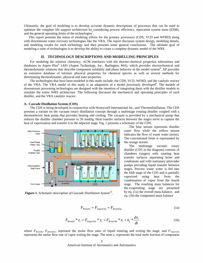
The CDS is being developed in conjunction with Honeywell International Inc. and Thermodistillation. The CDS presents a variant on the vacuum rotary distillation concept through a multistage rotating distiller coupled with a thermoelectric heat pump that provides heating and cooling. The vacuum is provided by a mechanical pump that reduces the distiller chamber pressure to 50 mmHg. Heat transfer surfaces between the stages serve to capture the heat of vaporization and transfer it to the adjacent stage. Fig. 1 presents a schematic of the CDS.

The blue stream represents distiller water flow while the yellow stream indicates the flow of waste water (urine). The concentrated brine is represented by the orange stream. The multistage vacuum rotary distiller (CD5 in the diagram) consists of chambers (stages) with rotating heat transfer surfaces separating brine and condensate and with stationary pitot-tube pumps providing liquid transfer between stages. Process waste water is fed into the fifth stage of the CD5 and is partially vaporized using heat from the condensation of vapor from the fourth stage. The resulting mass balances for the evaporating stage are presented by eq. (1a) the overall mass balance, and eq. (1b) the component mass balance

BrineOutVaporOutBrineIn FFF += (1a)

dtdxnxFyFzF i

LiBrineOutiVaporOutiBrineIn **** ++= (1b)

where FBrineIn, FBrineOut, represent the molar flow rates of liquid entering and exiting the stage, and FVaporOut represents the molar flow rate of vapor exiting the stage. The term zi represents the total mole fraction of component

Figure 1. Schematic description of Cascade Distillation System10.


4

i entering the stage, xi represents the liquid phase mole fraction of component i (in stream FBrineOut) and yi represents the vapor phase mole fraction of component i (in stream FVaporOut). The term nL

The resulting mass balances for the condensing stage are presented by eq. (2a), the overall mass balance and eq. (2b), the component mass balance

represents a fixed amount of liquid holdup within the stage. The evaporator stages are modeled as pseudo steady-state with a fixed holdup. The partitioning of components between liquid and vapor phase is calculated using the Aspen flash routine pflash2. The routine assumes that the stages have reached thermal equilibrium.

CondOutCondInVaporIn FFF =+ (2a)

iCondOutiCondIniVaporIn xFzFzF *** =+ (2b) where FCondIn, FCondOut, represent the molar flow rates of liquid entering and exiting the stage, and FVaporIn represents the molar flow rate of vapor entering the stage. The term zi represents the total mole fraction of component i entering the stage and xi represents the liquid phase mole fraction of component i (in stream FCondOut

Countercurrent flow of brine and vapor/condensate occur as a result of heating the most concentrated brine in the first stage. This leads to a temperature gradient between stages, increasing in the direction of brine flow and decreasing in the direction of condensate flow. The heat of vaporization is captured by heat transfer surfaces within the stages and used to heat the liquid in the next stage. Equations (3a) and (3b) present the energy balances for the evaporating and condensing stages respectively

). Similar to the evaporator stages, the condensing stages are modeled as pseudo steady-state. The partitioning of components between liquid and vapor phase is calculated using the Aspen flash routine pflash2. The routine assumes that the stages have reached thermal equilibrium.

BrineOutlVaporOutvBrineInBrineIn FhFhQFh *** +=+ (3a)

where hv, hl, represent the molar enthalpy liquid and vapor phases (calculated by pflash2), and hBrineIn represents the molar enthalpy of FBrineIn

, and Q represents the heat flow into the evaporator (heat of condensation recovered from the condensing stage)

QFhFhFh CondOutlVaporInVaporInCondInCondIn +=+ *** (3b)

where hl, represents the molar enthalpy liquid (calculated by pflash2) and hVaporIn, hCondIn represent the molar enthalpy of FVaporIn and FCondIn

Heat energy for the process is supplied by a thermoelectric heat pump (THP)

, respectively. Q represents the heat of condensation that is transferred to the evaporating stage. Once the brine has reached a maximum concentration, it is fed into a separate holding tank. A cooled condenser stage provides final condensate collection.

11

. The thermoelectric effect relies on using an electrically powered device to draw heat from a flowing stream. In the case of the CDS a portion of the liquid from stage one is fed to the heat pump and then recirculated back to the distiller to supply heat for the process. This heat energy is drawn from a portion of the recovered water as a recirculating water stream. Equations (4a) and (4b) present the governing equations for the THP

WQQ ch += (4a)

WQCOP h= (4b)

where the coefficient of performance (COP), describes the “efficiency” of the thermoelectric device, and Qc, Qh

The THP itself requires less power than a traditional heater, and since it uses thermal energy from the cold side to heat the hot side, it functions as both the condenser and the reboiler. The energy balances for the hot and cold sides of the THP are presented by eqs. (5a) and (5b) respectively

represent the heat flow from the cold stream and to the hot stream respectively.


5

HsideOutHsideOuthHsideInHsideIn FhQFh ** =+ (5a)

cCsideOutCsideOutCsideInCsideIn QFhFh += ** (5b) where hHsideIn, hHsideOut represent the molar enthalpy of FHsideIn, FHsideOut, (the streams entering and exiting the hot side of the THP) respectively. The terms hCsideIn and hCsideOut represent the molar enthalpy of FCsideIn and FCsideOut

Since the THP generates heat from electrical resistance within the device, a trim cooler (TC) is used to remove the additional heat from the cold recirculating stream. The TC is modeled as a single-pass heat exchanger that compensates for cooling inefficiencies of the THP. Reducing the pressure inside the distiller using the vacuum pump reduces the distillation temperature thus reducing power requirements even further

(the streams entering and exiting the cold side of the THP) respectively.

1

B. Vapor Compression Distillation

.

The VCD system is a single-stage distillation process that has been developed at Marshall Space Flight Center for the International Space Station (ISS). The distillation assembly, the primary component of the Vapor Compression Distillation system, appears in Fig. 2

Wastewater is deposited in a thin film along the inner evaporator surface of the rotating drum. As water

evaporates, it is pulled into the compressor through the hollow stationary shaft. The mass balances for this process are shown by eq. (6a) the overall mass balance, and eq. (6b) the component mass balance

BrineOutVaporOutBrineIn FFF += (6a)

dtdxnxFyFzF i

LiBrineOutiVaporOutiBrineIn **** ++= (6b)

where FBrineIn, FBrineOut, represent the molar flow rates of liquid entering and exiting the stage, and FVaporOut represents the molar flow rate of vapor exiting the stage. The term zi represents the total mole fraction of component i entering the stage, xi represents the liquid phase mole fraction of component i (in stream FBrineOut) and yi represents the vapor phase mole fraction of component i (in stream FVaporOut). The term nL represents a fixed amount of liquid holdup within the stage. The evaporator stages are modeled as pseudo steady-state with a fixed holdup. The

Figure 2. VCD distillation assembly schematic detailing internal components and process streams 12.


6

partitioning of components between liquid and vapor phase is calculated using the Aspen flash routine pflash2. The routine assumes that the stages have reached thermal equilibrium.

The compressor raises the temperature and pressure of the water vapor, and the compressed vapor then passes into the condenser, where it condenses on the outer surface of the rotating drum, in thermal contact with the evaporator surface. The mass balances for this process are show by eq. (7a) the overall mass balance, and eq. (7b) the component mass balance

CondOutVaporOutVaporIn FFF += (7a)

iVaporOutiCondOutiVaporIn yFxFzF *** += (7b) where FVaporIn, FVaporOut, represent the molar flow rates of vapor entering and exiting the stage, and FCondOut represents the molar flow rate of liquid exiting the stage. The term zi represents the total mole fraction of component i entering the stage, xi represents the liquid phase mole fraction of component i (in stream FCondOut) and yi represents the vapor phase mole fraction of component i (in stream FVaporOut

The resulting heat flux from the condenser to the evaporator, driven by the saturation temperature difference, drives the further evaporation of water inside the evaporator, and the VCD process thus recovers the latent heat of evaporation/condensation. Equations (8a) – (8c) describe the heat transfer process

). The partitioning of components between liquid and vapor phase is calculated using the Aspen flash routine pflash2. The routine assumes that the stages have reached thermal equilibrium.

BrineOutlVaporOutvBrineInBrineIn FhFhQFh *** +=+ (8a)

QFhFhFh VaporOutvCondOutlVaporInVaporIn ++= *** (8b)

TUAQ ∆= (8c)

For the evaporating process FBrineIn, FBrineOut, represent the molar flow rates of liquid entering and exiting the process and FVaporOut, represents the molar flow rate of vapor exiting the process. The terms hv, hl represent molar enthalpies of the vapor and liquid phases, calculated by pflash2. For the condensing process FVaporIn, FVaporOut, represent the molar flow rates of vapor entering and exiting the process and FCondOut, represents the molar flow rate of liquid exiting the process. The terms hv, hl

The evaporator pickup tube (Recycle Out) collects the wastewater not evaporated inside the evaporator. This concentrated wastewater (brine) flows through a recycle loop and is mixed with fresh wastewater for reprocessing. The condensed water vapor is collected from the condenser by the product water pickup tube (Product Out). The condenser is periodically purged (Purge Out) to remove non-condensable gases and to maintain the operating pressure.

represent molar enthalpies of the vapor and liquid phases, calculated by pflash2. The term Q represents the heat transferred. The term U represents the overall heat transfer coefficient (an assumed value) and A represents the surface area for heat transfer. The temperature difference (∆T) is the difference between the saturation temperature for evaporation and condensation.

The VCD evaporator process nominally operates at 3.4 to 5.5 kPa (0.5 to 0.8 psia) and 32 to 43°C ( 90 to 110°F). For further descriptions of the VCD process and system, including other components such as fluids pumps, the recycle filter tank, etc., are provided elsewhere12,13

C. Wiped Film Rotating Disk (WFRD)

.

Thin film distillation offers improved efficiency by enhancing heat transfer. In the WFRD system, a preheated feed is sprayed onto a rotating hollow disk assembly to create a thin film. The film evaporates quickly and the vapor is compressed and fed into the condenser section (the inside of the hollow disk assembly) of the unit. The heat of condensation is transferred back to the evaporating film hence conserving some energy. The overall process consumes less energy than a traditional distillation system. In essence the film evaporates via a combined convection/conduction process. Fig. 3 presents a schematic for the WFRD evaporator assembly (3a) along with the process flow diagram for the entire system (3b).


7

The basic operation for distillation within the WFRD can be summarized by Fig. 3. The hot feed is sprayed onto

the hollow rotating disk within the partially evacuated still. As the fluid evaporates it is pumped out through the “vapor out” port and fed into the inside portion of the hollow rotating disk through the “heating steam” port. The process can be described by the following equations

BrineOutVaporOutFeedIn FFF += (9a)

dtdxnxFyFzF i

LiBrineOutiVaporOutiFeedIn **** ++= (9b)

FeedmfilmrotorL dAn ,** ρ= (9c) where FBrineIn, FBrineOut, represent the molar flow rates of liquid entering and exiting the stage, and FVaporOut represents the molar flow rate of vapor exiting the stage. The term zi represents the total mole fraction of component i entering the stage, xi represents the liquid phase mole fraction of component i (in stream FBrineOut) and yi represents the vapor phase mole fraction of component i (in stream FVaporOut

In this model n).

L, the liquid holdup within the stage, is not a fixed value and is calculated by the mass balance. The important operating parameter in this case is the film thickness, dfilm, which is calculated based on the holdup and assuming a cylindrical geometry of the liquid layer. The average liquid density, ρm,Feed

The vapor is moved from the outside of the rotating disk to the inside using an external compressor. The mass balances for this process are described by eqs. (10a) – (10c) below

, is calculated using an Aspen procedure. The partitioning of components between liquid and vapor phase is calculated using the Aspen flash routine pflash2. The routine assumes that the stages have reached thermal equilibrium.

CondOutVaporOutVaporIn FFF += (10a)

dtdxnyFxFzF i

liVaporOutiCondOutiVaporIn **** ++= (10b)

Figure 3. Schematic representation of WFRD system. (A) WFRD Evaporator Assembly and (B) Process Schematic14.


8

FeedmfilmrotorL dAn ,** ρ= (10c)

where FVaporIn, FVaporOut, represent the molar flow rates of vapor entering and exiting the stage, and FCondOut represents the molar flow rate of liquid exiting the stage. The term zi represents the total mole fraction of component i entering the stage, xi represents the liquid phase mole fraction of component i (in stream FCondOut) and yi represents the vapor phase mole fraction of component i (in stream FVaporOut

As with the evaporator model described above, n).

l, the liquid holdup within the stage, is not a fixed value and is calculated by the mass balance. The film thickness, dfilm, is calculated based on the holdup, assuming a cylindrical geometry of the liquid layer. The average liquid density, ρm,Feed

As the vapor condenses, the heat of condensation is conducted through the wall of the rotating disk assembly and used to evaporate more of the feed. This combination of processes results in efficient evaporation with low power consumption. The process is described by the following system of energy balance equations

, is calculated using an Aspen procedure. The partitioning of components between liquid and vapor phase is calculated using the Aspen flash routine pflash2. The routine assumes that the stages have reached thermal equilibrium.

BrineOutlVaporOutvFeedInFeedIn FhFhQFh *** +=+ (11a)

QFhFhFh VaporOutvCondOutlVaporInVaporIn ++= *** (11b)

TUAQ ∆= (11c)

)( filmdfU = (11d)

For the evaporating side FFeedIn, FBrineOut, represent the molar flow rates of liquid entering and exiting the evaporator side, and FVaporOut represents the exiting molar flow rate of vapor. The terms hv, hl represent molar enthalpies of the vapor and liquid phases, calculated by pflash2. For the condensing side FVaporIn, FVaporOut, represent the molar flow rates of vapor entering and exiting the process and FCondOut, represents the molar flow rate of liquid exiting the process. The terms hv, hl

Feed that is not evaporated becomes enriched with waste byproducts while the vapor consists primarily of water and volatile gases. The enriched brine is disposed through the brine scoops on the outside of the rotating disks while the collected distillate (pure water) is sent to the distillate tank through a product tube.

represent molar enthalpies of the vapor and liquid phases, calculated by pflash2. The term Q represents the heat transferred. The term U represents the overall heat transfer coefficient and A represents the surface area for heat transfer. The temperature difference (∆T) is the difference between the temperatures for evaporation and condensation. Fundamental to the wiped film evaporator technology, U is a function of the resistances from the evaporating film, the condensing film, and the rotor.

As mentioned earlier, the evaporated feed (vapor) is moved from the outside portion of the hollow rotating disk assembly to the inside of the hollow disk where it is condensed. The external compressor is shown in Fig. 3b. Fig. 3b also shows the flow paths for the brine and distillate collection. It is also worth noting the integration of various streams for heat exchange. For example, feed is heated by the hot brine exiting the evaporator loop and heated again by the hot liquid product exiting the condenser. This heat exchanged between hot and cold streams provides substantial savings in operational power.


9

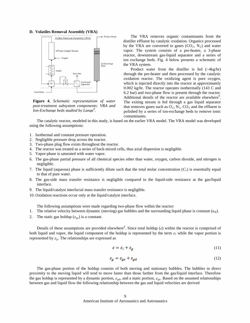
D. Volatiles Removal Assembly (VRA) The VRA removes organic contaminants from the distiller effluent by catalytic oxidation. Organics processed by the VRA are converted to gases (CO2, N2

Product water from the distiller is fed (~4kg/hr) through the pre-heater and then processed by the catalytic oxidation reactor. The oxidizing agent is pure oxygen, which is injected directly into the reactor at approximately 0.002 kg/hr. The reactor operates isothermally (143 C and 6.2 bar) and two-phase flow is present through the reactor. Additional details of the reactor are available elsewhere

) and water vapor. The system consists of a pre-heater, a 3-phase reactor, downstream gas-liquid separator and a series of ion exchange beds. Fig. 4 below presents a schematic of the VRA system.

9. The exiting stream is fed through a gas liquid separator that removes gases such as O2, N2, CO2

The catalytic reactor, modeled in this study, is based on the earlier VRA model. The VRA model was developed using the following assumptions:

and the effluent is polished by a series of ion-exchange beds to remove ionic contaminants.

1. Isothermal and constant pressure operation. 2. Negligible pressure drop across the reactor. 3. Two-phase plug flow exists throughout the reactor. 4. The reactor was treated as a series of back-mixed cells, thus axial dispersion is negligible. 5. Vapor-phase is saturated with water vapor. 6. The gas-phase partial pressure of all chemical species other than water, oxygen, carbon dioxide, and nitrogen is

negligible. 7. The liquid (aqueous) phase is sufficiently dilute such that the total molar concentration (Cl

8. The gas-side mass transfer resistance is negligible compared to the liquid-side resistance at the gas/liquid interface.

) is essentially equal to that of pure water.

9. The liquid/catalyst interfacial mass transfer resistance is negligible. 10. Oxidation reactions occur only at the liquid/catalyst interface.

The following assumptions were made regarding two-phase flow within the reactor: 1. The relative velocity between dynamic (moving) gas bubbles and the surrounding liquid phase is constant (uB

2. The static gas holdup (ε).

gs

) is a constant.

Details of these assumptions are provided elsewhere9. Since total holdup (ε) within the reactor is comprised of both liquid and vapor, the liquid component of the holdup is represented by the term ε l while the vapor portion is represented by εg

. The relationships are expressed as

(11)

(12)

The gas-phase portion of the holdup consists of both moving and stationary bubbles. The bubbles in direct proximity to the moving liquid will tend to move faster than those farther from the gas/liquid interface. Therefore the gas holdup is represented by a dynamic portion, εgd, and a static portion, εgs. Based on the assumed relationships between gas and liquid flow the following relationship between the gas and liquid velocities are derived

Figure 4. Schematic representatiom of water post-treatment subsystem components: VRA and Ion-Exchange beds studied by Lange9.


10

)( g

l

gd

gB

uuu

εεε −−= (13)

where ul and ug

are the liquid and gas phase velocities. Based on assumption 5 and the definition of the total holdup, the overall gas phase mass balance becomes

∑=

−−−=−gn

iij

jOH

cs

gjOHg J

dzGd

yAdt

dyC

2

)()1(1)1(

22

ε (14a)

PTp

y OHOH

)(02

2= (14b)

and the overall mass balance over both phases becomes

∑=

+

+−=

−

pn

iij

jj

cs

gjlg R

dzdL

dzdG

Adtd

CC1

1)(ε

(15)

where Cl is the liquid phase total molar concentration, Cg is the gas phase molar concentration (assumes ideal gas), Gj is the total gas phase mass flow rate, Lj is the total liquid phase mass flow rate, yH2O is the vapor phase mole fraction of water (which is constant due to assumption 5), and Acs is the reactor cross-sectional area. The summation terms represent total flux (vapor to liquid phase), Jij, and total consumption/generation by chemical reaction, Rij, respectively and np represents the number of reacting species. The subscript j identifies the position along the length of the reactor (the z-axis). Based on assumptions 5 and 6, eqs. (14a) and (14b) pertain only to the major gas phase components CO2, N2, O2, and H2O and ng represents the number of gas phase components. Per eq. (14b), yH2O is solely a function of reactor pressure P, and reactor temperature T and p0

H2O

Equations (16) and (17) are used to describe the component mass balances in the vapor and liquid phases

(T) represents the saturation vapor pressure of water at T (calculated by Antoine’s equation).

ijjij

cs

ijgjg J

dzGyd

Adtyd

C −−=)(1)(ε

(16)

ijijjij

cs

ijljl RJ

dzLxd

Adtxd

C ++−=)(1)(ε

(17)

where yij is the gas phase mole fraction of component i, and xij is the total liquid mole fraction of component i. The reaction rate Rij was calculated using the Aspen Reactions Toolkit

R rij ki kjk

nr

==∑σ

1

4

(18)

where rkj is the individual rate of surface reaction and σkj is the stoichiometric coefficient for each species in each reaction k. The model assumes that the rate of each catalytic surface reaction can be described by a general Langmuir-Hinshelwood-Hougen-Watson expression15


11

rk x

K x

kj

sk ijn

i

n

i iji

n m

ki

r

i

tk

=

+

=

=

∏

∑

( )

( )

2

21 ν

(19)

where ksk is a rate constant for reaction k, Ki is an effective adsorption equilibrium constant for species i, and nki, ν i, and mk are constant exponents. For the VRA model, all nki and ν i have been set equal to 1. The effective adsorption equilibrium constant for species i was set to zero except for oxygen (Ki = 1.17e06) and mk was set to two. The reaction rate constants were identical to those used by the previous VRA model9

Since the primary resistance to gas/liquid interfacial mass transfer resides in the liquid phase (assumption 8), the following expression describes the flux of gaseous species into the liquid phase

.

)( *

ijijllijij xxaCkJ −=

(20) where klija is the liquid-side mass transfer coefficient for species i, and xij

* is the liquid-phase mole fraction of i in equilibrium with the gas phase in cell j. This flux expression pertains to three gas phase components CO2, N2, O2

The term x.

ij*, is an equilibrium term and can therefore be calculated by equilibrium thermodynamics. In this

case xij* is calculated using the pflash2 routine assuming fixed reactor P, T and yij being determined from the mass

balance. Using the Aspen flash routines accounts for pH related changes in solubility and speciation (significant for CO2

The mass transfer resistance, k

dissolution) and automatically accounts for temperature effects allowing the model to be adapted for a wider range of temperatures and pressures.

lija

can be expressed in the following form:

[ ]2/13/12/13/12 )(82.023.026 bdigsgjbsjigsgj

b

lilij ReScReSc

dDak εεεε −++= (21)

with

lli

li D

Scρ

µ=

(22)

)( gjl

lljbbsj

udRe

εεµρ−

= (23)

and

l

lBbbd

udReµρ

= (24)

where Sc and Reb are the dimensionless Schmidt and bubble Reynolds numbers, respectively, db is the bubble diameter, Dl is the liquid-phase diffusion coefficient, µl is the liquid-phase dynamic viscosity and ρl is the liquid density. The bubble diameter was fixed while the fluid transport parameters (Dl, ρ l, µl

The mass transfer resistance incorporates both static components and dynamic components, since some gas bubbles are moving while others remain stationary. Therefore Re

) were calculated by procedures within ACM.

bd pertains to the dynamic bubbles while Rebs pertains to the static bubbles. Equation (21) is based on the widely used correlation by Frößling16. The development of the mass transfer resistance correlation as pertains to the VRA is discussed elsewhere9.


12

Given the system of equations and relationships, a first-order backward finite difference discretization scheme (BFD1) and Gear integration method were used to solve the model equations4. The reactor was discretized into 20 differential volumes of length dz and cross sectional area Acs

III. Results and Discussion

. The integration method and discretization schemes are built-in features of the ACM software.

The main focus of this study was to demonstrate the dynamic simulation capabilities of the various models that were developed. The simulation results for the distiller models were compared to data from the Distillation Comparison Test14,17,18. Because this study emphasized dynamic modeling, the comparisons were made between temperatures and pressures within the distillers. Steady-state solution chemistry results are also presented. The results from the distiller modeling were presented earlier this year19. The simulation results for the ACM VRA model were compared to results from the previous VRA model as well as test data19

A. Cascade Distillation System

. In this case steady-state conversion of organics was used as a comparison metric.

Fig. 5 presents the ACM flowsheet for the CDS. The CDS process simulation includes a number of models for individual components of the system. The multistage rotary vacuum distiller is modeled as a number of stages; five evaporating stages and five condenser stages. Each evaporator stage passes evaporated water to the adjacent condenser stage and the heat of condensation is passed to that stage’s evaporator (except for stage 1).

Since the CDS model consists of several evaporating and condensing stages, it is possible to track temperatures and pressures for each stage within the rotating distiller. The model is capable of identifying temperature and pressure gradients within the evaporating stages of the distiller. Fig. 6 presents the temperatures and pressures of the five evaporating stages. These temperatures are plotted along with test data for the temperatures of the hot loop exiting and entering the distiller (6a). The pressures are plotted along with the operating pressure of the rotating distiller that was observed during the test runs (6b).

Figure 6. CDS dynamic results (A) evaporator temperatures (B) evaporator pressures plotted along with test data19.

Figure 5. ACM flowsheet model of the CDS. The multistage rotary-vacuum distiller is represented by five evaporator and five compressor stages.


13

Fig. 6b shows reasonable agreement between model predictions and test as seen with the close correspondence between the model prediction of the stage 5 pressure and the experimental data. The cyclic behavior shown in the test data is characteristic of the CDS operation in that the vacuum system maintains a consistent internal pressure. As the solution is distilled, the increase of water and gases in the vapor phase increases the internal pressure. Once the internal pressure reaches a certain point, the system activates the vacuum pump to reduce the internal pressure. The model does not incorporate such a feature, but it can be implemented using a series of commands called tasks. The results in Fig. 6b demonstrate that the thermodynamic calculations capture most of the physics of the distillation process.

However, Fig. 6a shows poor agreement between the model’s prediction and the test results with regards to distiller temperatures. If the model parameters are tuned correctly, the temperature of the evaporator stage 1 should be approximately equal to DCT Data ‘CD Out/THP In.’ Since the evaporator stage 1 temperature lies outside the experimentally determined range of hot loop temperatures, it was suspected that the THP needed to be re-evaluated. Fig. 7 presents the predicted inlet and outlet temperatures for the THP hot loop against the experimentally determined hot loop temperatures. The figure presents temperature predictions based on a COP value of 2.0 and 1.5.

Based on the alignment of the data to the model (the dashed lines), the results suggest that a COP of 1.5 may correlate better to the test performance. However, since the documented COP of the THP is closer to 2.3, it is apparent that some inefficiency in the THP is not being incorporated into the model equations.

The chemistry within the process simulation is based on thermodynamic data generated by AP and all aqueous components are tracked during mass balance calculations as neutral (apparent) species as opposed to ionic species. Vapor-liquid equilibrium calculations are performed using actual true-component compositions. Fig. 8 presents the urea mole fraction (XUrea

As expected, the highest urea concentration was predicted at stage 1, the stage closest to the brine recirculation loop, with the lowest values predicted for stage 5. The simulation models the successive enriching of the brine in stage 1 by the slow removal of water from the waste input stream. Similar calculations can be generated for the condenser side components. Concentrations of any individual liquid phase species can be tracked in a similar fashion.

), within each of the five evaporator stages of the CDS.

Additional information can be garnered based on the feed chemistry model used in the simulation. For example, the DCT feed incorporates solid formation in parts of the CDS such as the feed tank and the evaporator sections. Solids formation is not calculated in the condenser blocks and the product tank since solids would be very unlikely to form, as only water vapor and gases reach the condenser

Figure 7. Model predictions for THP hot loop inlet and outlet temperatures along with test data for COP = 2.0 and COP = 1.519.

Figure 8. Variation of urea concentration in the evaporator stages of the CDS. Stage 1 corresponds to the stage closest to the brine recirculating loop and therefore accumulates the highest concentration of brine. Stage 5 lies closest to the distillate final condenser and therefore accumulates the least amount of brine19.


14

blocks. In addition to dynamic modeling, this study assessed model performance by examining steady-state predictions of stream chemistry, production rate and energy consumption. The steady-state comparisons are compiled in Table 1. The model results assumed an ersatz chemistry for the feed model, while the DCT results were based on solution 1 chemistry (urine + humidity condensate).

Stream chemistry, pH in particular, showed reasonable agreement between the DCT and the modeling results. For the feed stream and distillate streams, the pH variation between the model and the test was small (~10%). The large discrepancy in the brine stream pH between model and experiment may be caused by a difference in operating conditions rather than a mismatch in the chemistry prediction. In the model, brine is allowed to accumulate in stage 1, while in the actual CDS unit, the brine accumulates elsewhere. Small to marginal deviations in stream chemistry are expected since the model uses only a portion of the components detected during The DCT. Using percent deviation is not

meaningful for temperature comparisons, and therefore Table 1 shows temperature difference for deviation for temperature properties. In terms of operating conditions, the model predicts a production rate of 4.26 kg/hr, which is close to the production rate (4.04 kg/hr) seen during the test. Unlike the test, the model predicts the production rate based on the extraction of water (calculated by VLE thermodynamics) so the close alignment between model and test further validates that Aspen’s flash routine is appropriate for this distillation model. Similar to the test operational scheme, the model specifies a fixed electrical input to the THP in order to control the respective heating and cooling of the the hot and cold sides. Given the good prediction of the production rate, by the model, the results show good agreement between the THP specific energy consumption predicted by the model and observed in the test data. The model does not incorporate energy consumption by the rotating distiller so the specific energy consumption values are only pertinent to the THP operation.

B. Vapor Compression Distiller Several updates to the VCD model have been

incorporated since previous reports on distillation model development5,19

The dynamic study for the VCD incorporated several aspects focusing on the distillation assembly. Close examination of the temperature profiles within the distiller (Fig. 10a) showed close trending behavior between the ambient temperature and the thermal behavior of the VCD. Also, there appeared to be a correlation between pressures and temperatures within the distillation assembly (DA), and power consumption of the DA (Fig. 10b) since an external heater was used to eliminate the presence of entrained liquid. Fig. 11 presents an engineering schematic of the unit.

. Fig. 9 presents an ACM flowsheet of the VCD system. The current model includes the recycle filter tank assembly (RFTA) and the heat exchanger upstream of the DA_evaporator (part of the distillation assembly).

Figure 9. ACM flowsheet model of Vapor Compression Distillation system19.

Table 1. CDS Steady-State Results vs. DCT Data19

Property DCT Data Model Deviation

Production Rate (kg/hr) 4.06 4.26 4.93% THP specific energy (W-hr/kg) 70.5 70.67 0.24% Feed pH 2.22 2.07 -6.76% Brine pH 1.65 1.1 -33.33% Distillate pH 4.03 3.5 -13.15% COP 2.3 2.0 -13.04% Hot Loop THP/Out CD In (C) 43 50.43 7.4 Hot Loop THP In/CD Out (C) 36 44.47 8.5 Cold Loop CD Out/THP In (C) 22.5 23 0.5 Cold Loop CD In/ HX Out (C) 20.5 17.5 -3.0


15

Given this detailed, highly dynamic set of test

results, the modeling approach encompassed the development of a simulated heater profile and a dynamic run to compare temperature and pressure profiles within the distiller. Fig. 12 compares thermal behavior between model and test while Fig. 13 compares pressures.

Estimates of the internal temperature and pressures provided by Figs. 12b and 13b respectively show reasonable agreement with the DCT results. Modeling the Heater Profile was achieved through tasks in Aspen Custom Modeler and the resulting dynamic behavior shows good agreement between model and test.

Figure 10. VCD thermal behavior (A) normal-mode temperatures over 32 days) and (B) Day 7 temperatures vs. distillation assembly heater profile19.

Figure 11. VCD System Schematic20.

Figure 12. Dynamic temperatures vs. heater power profiles for (A) day 7 temperatures from DCT and (B) model predictions of temperatures for day 719.


16

C. Wiped Film Rotating Disk In this study, the WRFD model (Fig. 14) was simplified in that it used the ersatz feed chemistry and eliminated

the recycle stream from the evaporator side model. Also elements of the condenser side model were tuned to more closely align with the test and the true operation of the hardware. Simplifying the feed chemistry also improved convergence of the model.

The dynamic modeling for the WFRD centered upon testing the agreement between pressure and temperature profile predictions and test data. Some of the operating parameters, such as the evaporator pressure, compressor operation, and processing rates were fixed values, similar to those used in the DCT.

Fig. 15 provides the internal pressure and temperature profiles (based on the DCT data) along with model predictions. Although good agreement between model and test is demonstrated in Fig. 15a significant deviations are seen in the temperature profiles (Fig. 15b). This may be due to an inefficiency within the system that was not captured by the model. In particular, there may be a time dependent build-up of film that decreases the heat transfer efficiency between the condensing and evaporating sides, thus leading to an increasing temperature difference between the condensing and evaporating sides. The WFRD model assumes a fixed film thickness for both the condenser and the evaporator during operation, an assumption that may not capture the complete physics of the WFRD.

Figure 13. Dynamic pressures vs. heater power profiles for (A) day 7 pressures from DCT and (B) model predictions of distillation assembly internal pressure for day 719.

Figure 14. ACM representation of the Wiped Film Rotating Disk system.

Figure 15. WFRD dynamic results (A) system internal pressures (B) system internal temperatures, plotted along with DCT results19.


17

In addition to dynamic modeling, this study assessed model performance by examining steady-state predictions of stream chemistry, production rate, and energy consumption. The steady-state comparisons are compiled in Table 2. The model results assumed an ersatz chemistry for the feed model, while the DCT results were based on solution 1 chemistry (urine + humidity condensate). Percent deviation is not meaningful for temperature comparisons, and therefore Table 2 shows temperature difference for deviation for temperature properties.

Specific energy consumption predicted by the model (for the compressor) was high (34 W-hr/kg) when compared to the test results (~25 W-hr/kg) which is perhaps a result of the model used for the compressor. However, there is a significant improvement between the predictions of the current model vs. the previous model5

D. Volatiles Removal Assembly

. Stream chemistry predictions show reasonable agreement with DCT results.

The approach for developing, testing and validating the VRA model was significantly different than what was applied towards distillation modeling. For the VRA model, the main development goals included applying Aspen’s capabilities and built-in functions to simplify the model development and checking the solution against the previously developed model9 and available single component test data21. The two capabilities incorporated from Aspen include flash calculation methods and the Aspen Reactions Toolkit (ART)4

ART provides a convenient system for inputting and managing a set of reaction chemistries. As opposed to the FORTRAN language implementation, which relied on hard-coded sets of matrices and database files that represent the reaction stoichiometries and kinetic parameters, ART consolidates this information into one data set (called a structure) and includes an organized graphical user-interface (GUI). Reactions can be updated, activated or de-activated using the GUI

.

4

Aspen flash procedures perform thermodynamic calculations using external FORTRAN routines. The flash routines were used to calculate equilibrium solubility of gases in the liquid phase of the reactor. These equilibrium points were used to calculate the mass transfer driving force for each gas species and calculate gas flux. The FORTRAN version of the VRA model used assumed values for Henry’s law coefficients to calculate the equilibrium liquid-phase concentrations. To account for pH effects on H

.

2O-CO2(aq) equilibrium, the model also included a special calculation to adjust the Henry’s law coefficient for CO2. Using the Aspen flash routines automatically incorporated the pH effect (for CO2

Using the flash routine improved model performance and stability, by allowing Aspen to calculate the equilibrium conditions outside of the main simulation, and reducing the required number of calculations at each step.

) along with temperature dependencies on gas solubility and minor adjustments for the mixed component liquid phase (vs. assuming pure water as the liquid phase).

To test the model performance the results were compared to results from the FORTRAN model along with the original test data. Comparisons of calculated mass transfer coefficients, transport properties and liquid phase

Table 2. WFRD Steady-State Results vs. DCT Data19

Property DCT Data Model Deviation

P, Compressor In (torr) 82 80 -2.44% P, Compressor Out (torr) 110 109.8 -0.18% T, Evaporator Out (C) 52.6 47.84 -4.76 C T, Condenser Out (C) 65.3 53.4 -11.9 C compressor specific energy (W-hr/kg) 25 33.9 35.60% Feed pH 2.25 2.07 -7.56% Distillate pH 3.5 3.21 -8.45% Brine pH 1.8 1.53 -15.08%

Figure 16. Comparison of reactor model predictions to VRA data and previous modeling results for ethanol oxidation at a reactor temperature of 126.7ºC22.


18

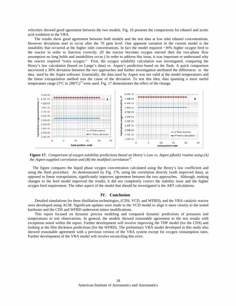
velocities showed good agreement between the two models. Fig. 16 presents the comparisons for ethanol and acetic acid oxidation in the VRA. The results show good agreement between both models and the test data at low inlet ethanol concentrations. However deviations start to occur after the 70 ppm level. One apparent variation in the current model is the instability that occurred at the higher inlet concentrations. In fact the model required ~30% higher oxygen feed to the reactor in order to function correctly. (If the reactor becomes oxygen starved then the two-phase flow assumption no long holds and instabilities occur.) In order to address this issue, it was important to understand why the reactor required “extra oxygen.” First, the oxygen solubility calculation was investigated, comparing the Henry’s law calculation (based on Lange’s data) vs. Aspen’s prediction based on the flash. A quick comparison uncovered a 30% deviation between the two approaches and further investigation attributed the differences to the data used by the Aspen software. Essentially, the data used by Aspen was not valid at the model temperatures and the linear extrapolation method was the cause of the deviation. To test this idea, data spanning a more useful temperature range (3°C to 288°C)23

were used. Fig. 17 demonstrates the effect of the change.

The figure compares the liquid phase oxygen concentration calculated using the Henry’s law coefficient and using the flash procedure. As demonstrated by Fig. 17b, using the correlation directly (with improved data), as opposed to linear extrapolation, significantly improves agreement between the two approaches. Although, making changes to the feed model improved the results, it did not completely correct the stability issue and the higher oxygen feed requirement. The other aspect of the model that should be investigated is the ART calculations.

IV. Conclusion Detailed simulations for three distillation technologies, (CDS, VCD, and WFRD), and the VRA catalytic reactor

were developed using ACM. Significant updates were made to the VCD model to align it more closely to the tested hardware and the CDS and WFRD underwent minor modifications.

This report focused on dynamic process modeling and compared dynamic predictions of pressures and temperatures to test observations. In general, the models showed reasonable agreement to the test results with exceptions noted within the report. Further development will involve improving the THP model (for the CDS) and looking at the film thickness predictions (for the WFRD). The preliminary VRA model developed in this study also showed reasonable agreement with a previous version of the VRA system except for oxygen consumption rates. Further development of the VRA model will involve reconciling this error.

Figure 17. Comparison of oxygen solubility predictions based on Henry’s Law vs. Aspen pflash2 routine using (A) the Aspen-supplied correlation and (B) the modified correlation22.


19

Acknowledgments: The authors acknowledge continuing support from Life Support and Habitation Systems along with ongoing

contributions from hardware developers at various centers and institutions.

References 1. Rifert, V., Usenko, V, et al. (1999). Comparison of Secondary Water Processors Using Distillation for Space Applications. International Conference on Environmental Systems. Denver, CO USA. 2. Hermann, C. C. (1992). High-Recovery Low-Pressure Reverse Osmosis. 22nd International Conference on Environmental Systems, Seattle, WA USA 3. Akse, J. R., J. E. Atwater, et al., Eds. (1994). A Breadboard Electrochemical Water Recovery System for Producing Potable Water from Composite Wastewater Generated in Enclosed Habitats. Water Purification by Photocatalytic, Photochemical, and Electrochemical Processes, Electrochemical Society. 4. (2006). Aspen Custom Modeler v. 2006.5. Cambridge, MA, AspenTech. 5. Allada, R. (2008). Water Recovery Technology Development: 2008 Joint NASA/ESCG Report to SIMA, ESCG-4470-08-TEAN-DOC-0383, NASA Johnson Space Center, Houston, TX, October 2008. 6. Allada, R. (2010). Detailed Modeling of Advanced Distillation Technologies for Closed-Loop Water Recovery Systems, ESCG-4470-10-TEAN-DOC-0129, NASA Johnson Space Center, Houston, TX, September 2010. 7. Levri, J.A., Fisher, J.W., Jones, H.W., Drysdale, A.E., Hanford, A.J., Hogan, J.A., Joshi, J.A., Vaccari, D.A., Advanced Life Support Equivalent System Mass Guidelines Document, NASA/TM-2003-212278, NASA Ames Research Center, Moffet Field, CA, 2003.

8. (2006). Aspen Plus v. 2006.5. Cambridge, MA, AspenTech. 9. Lange, K. E. (1997). Development and Integration of a Detailed Model of the LMLSTP Volatile Removal Assembly (VRA) Water Post-Treatment Subsystem, HDID-A44B-717, NASA Johnson Space Center, Houston, TX, July 1997. 10. Lange, K. E. and J. P. Van Buskirk (2006). Transient Modeling of an Early Lunar Outpost Life Support System. Systems Integration Modeling and Analysis (SIMA). 11. Rifert, V., Usenko, V., et. al, (2001) Design Optimization of Cascade Rotary Distiller with the Heat Pump for Water Reclamation from Urine, International Conference on Environmental Systems. Colorado Springs, CO, USA. 12. Holder, D. W. and C.F. Hutchens. (2003). Development Status of the International Space Station Urine Processor Assembly. International Conference on Environmental Systems, Vancouver, British Columbia, Canada. 2003-01-2690. 13. Wieland, P., Hutchens, C., Long, D. and B. Salyer. (1998). Final Report on Life Testing of the Vapor Compression Distillation/Urine Processing Assembly (VCD/UPA) at the Marshall Space Flight Center (1993 to 1997). NASA/TM—1998-208539. 14. Crenwelge, L., McQuillan, J. (2009). Exploration Life Support Water Recovery System Distillation Comparison Test Plan. Houston, TX, NASA Johnson Space Center. 15. Carberry, J. J., Chemical and Catalytic Reaction Engineering, McGraw-Hill, New York, 1976. 16. Frößling, N., Gerlands Beitr. Geophys., 32 (1938) 170.

17. Allada, R. Yeh, H.Y, (2010). SIMA Analysis Report in Support of the Exploration Life Support Office Distillation Technology Down – Select, ESCG-4470-10-TEAN-DOC-0001-A, NASA Johnson Space Center, Houston, TX, February 2010.

18. McQuillian, J., K.D. Pickering et. al, (2010). Distillation Technology Down-selection for the Exploration Life Support (ELS) Water Recovery Systems Element. 40th International Conference on Environmental Systems, Barcelona, Spain


20

19. Allada, R. (2011). Modeling of Distillation Technologies for Wastewater Recovery, LSHS Special Topics Telecon, July 14, 2011. 20. Carter, D. L., and R. M. Bagdigian, “Vapor Compression Distillation Technology Report and Development Plan For the Exploration Life Support Project Distillation Technology Down-Selection,” MSFC, December 2010. 21. Dall-Bauman, L. A., personal communication, NASA Johnson Space Center, Houston, TX, April 30, 1996.

22. Allada, R. (2011). Dymanic Modeling of Process Technologies for Closed-Loop Water Recovery Systems, ESCG-4470-11-TEAN-DOC-0054, NASA Johnson Space Center, Houston, TX, September 2011. 23. Cramer, S.D., The Solubility of Oxygen in Brines from 0 to 300 °C, Ind. Eng. Chem. Process Des. Dev. 19, (1980), 300-305.

dynamic modeling of process technologies for closed-loop ... · american institute of aeronautics...

Documents