dynamic microeconomic models of fertility choice: a...

J Popul Econ (1997) 10:23–65

Dynamic microeconomic modelsof fertility choice: A survey

Cristino R. Arroyo 1, Junsen Zhang2

1Department of International Economics, Johns Hopkins University, Nitze School of Ad-vanced International Studies, 1740 Massachusetts Ave. NW, Washington, DC 20036-1984,USA(Fax: (202) 663-5683, e-mail: [email protected])2Department of Economics, Chinese University of Hong Kong, Shatin, NT, Hong Kong(Fax: (852) 2603-5805, e-mail: [email protected])

Received August 26, 1994/Accepted October 23, 1996

All correspondence to Junsen Zhang. The authors thank Chunrong Ai, Susan Cochrane, JohnGeweke, V. Joseph Hotz, Robert Miller, Ali Tasiran, and Kenneth Wolpin for providing uswith source material. We are also grateful to the anonymous referees, and the responsibleeditor of this journal for their encouragement and patience, and for contributing several help-ful suggestions that greatly increased the value-added of this paper. Any remaining errors arethe sole responsibility of the authors.Responsible editor:Klaus F. Zimmermann.

Abstract. We review existing approaches to the specification and estima-tion of dynamic microeconomic models of fertility. Dynamic fertility mod-els explain the evolution of fertility variates over the life-cycle as the solu-tion to a dynamic programming model involving economic choices. Dy-namic models may be classified into structural and reduced-form models.Structural models generally require solution of the underlying dynamic pro-gramming problem. Reduced-form models, while based on a structural spe-cification, do not. Recent innovations in estimation methodologies makeboth types practical and realistic alternatives to static models of lifetime fer-tility.

JEL classification: J13, C41, C61

Key words: Fertility, dynamic micro models

1. Introduction and motivation

This paper surveys dynamic microeconomic models of fertility choice thathave appeared in the recent literature. By dynamic models we mean ones thatexplicitly model thetime profileor intertemporal evolutionof fertility choice

and outcomes, as distinct from models that study once-and-for-all lifetime fer-tility decisions. Within the class of dynamic fertility models, we offer the fol-lowing general taxonomy. A model may be consideredstructural when itsestimable components require the specification and exact solution of an expli-cit dynamic maximization problem.Reduced-formdynamic models are thosewhich may estimate structural parameters or relationships arising from a dy-namic programming problem, but do not rely on the exact solution of the dy-namic equations. For instance, the form of a reduced-form model may be spe-cified in conformity with some tractable econometric framework not tied tothe exact form of the model’s solution. Our paper concentrates on thesetwo general approaches to analyzing fertility dynamics.1

To further sharpen our focus we survey onlyeconomicmodels of fertil-ity, i.e., models in which fertility variates are substantially outcomes of aneconomic choice process. This deliberately omits discussion of an impor-tant research program that studies fertility dynamics but which emphasizesbiological rather than economic determinants (i.e., the seminal work ofSheps and Menken 1973 and derivative papers). We neglect these models,but do so without prejudice to their valuable contributions. Finally, we alsoomit aggregative or macroeconomic models of fertility,2 even if these havemicrofoundations.

In relation to other surveys of this literature, this paper fills a gap that isnot covered by the recent surveys of Montgomery and Trussell (1984),Eckstein and Wolpin (1989), Rust (1994), and Olsen (1994). Olsen (1994)discusses several economic approaches to fertility notably what may becalled the Easterlinian, Schultzian, and Beckerian approaches after those re-spective authors. All of the approaches surveyed in Olsen lead to essen-tially static models of lifetime fertility choice.3 While not their sole empha-sis, the more technical surveys of Montgomery and Trussell, Eckstein andWolpin, and Rust (1994) issues relevant to the specification of dynamic fer-tility models. Eckstein and Wolpin, and Rust (1994) outline a general dy-namic framework that encompasses many discrete-choice models used inother research besides fertility. Like these studies, we cover generalapproaches, but our emphasis is specifically on dynamic fertility models.Montgomery and Trussell provide a more focused discussion of fertility is-sues, albeit in the context of the handful of dynamic models around at thetime. (They also give a good perspective of the relationship between life-cycle models of fertility against the research on lifetime fertility behaviorand female labor supply.) Our paper may be regarded as both an updatingof Montgomery and Trussel’s (1986) survey and an expansion upon the is-sues of dynamic specification and estimation.

Recent research has turned up many stylized empirical regularities witha time dimension.4 None of these facts can be adequately explained by amodel of lifetime fertility choice, however sophisticated, since lifetimefertility models lack a true time dimension. Treating fertility decisions asonce-and-for-all choices makes it difficult, if not impossible, to connect rea-lized fertility to variations in contraception costs, wages, income, education,mortality risks, or women’s labor market participation over time, nor canthese explain birth-timing or spacing. Recent efforts, consequently, have fo-cused on tractable models that incorporate fertility dynamics. This newwave of dynamic analysis reflects both the conscious attempt to overcome

24 C.R. Arroyo, J. Zhang

prior analytical limitations and the influence of methodological develop-ments in other areas of economics.

Dynamic approaches based on life-cycle choice represent a significantphilosophical departure from the traditional static view of the fertility deci-sion. Unlike the one-shot family size decision of static models, fertilitychoices over the life-cycle become a plan foreach time periodand eachcontingency(i.e., apolicy). Dynamic models also result in optimal fertilitypolicies that areforward-lookingand time-consistent.5

From an econometric standpoint two further differences may be noted.Structural dynamic models generally prespecify stochastic elementsas anintegral componentof the model, whereas lifetime choice models will intro-duce these directly into the estimating relations. This, however, can make abig difference not just for interpretation of the econometric estimates, butfor the appropriate choice of the estimator itself. Further, it makes more senseto imbed certain types of randomness in a dynamic setting; for instance, un-certainty about natural fecundity or preferences on family size can evolve asindividuals acquire fertility experience. Finally, to the extent that some staticmodels represent reduced-forms or time-aggregated versions of a dynamicmodel, information is lost in reducing or aggregating the model over time.When possible, estimation of a structural model can be more informative.

These considerations work in favor of dynamic life-cycle fertility mod-els. Counterbalancing these advantages, however, is the fact that, at thepresent juncture, the use of dynamic models still requires a trade-off be-tweenmodel realismand model tractability.This will become more appar-ent in the ensuing text.

Our paper is organized as follows. Section 2 studies a general frame-work nesting several well-known fertility models of the structural variety,including that of Heckman and Willis (1976), Wolpin (1984), Hotz andMiller (1984), Rosenzweig and Schultz (1985), Newman (1988), andLeung (1991). Section 2 also covers recent estimation/simulation techniquesthat have been proposed for structural models of the discrete-choice type.Section 3 reviews reduced-form models, focusing primarily on specificationand estimation issues of hazard-rate models and linear approximations tooptimal decision rules. Section 4 surveys other dynamic models that areneither structural nor reduced-form in nature.

2. Structural models

2.1 General framework

Introducing more general and “realistic” types of uncertainty, patterns of se-rial correlation, and time-variation with economic or biological variables re-quires an explicitly dynamic framework. Astructural approach (i) modelsobserved fertility as part of the solution of an explicit dynamic program-ming problem, and (ii) derives estimable or computable relationships fromthis solution.

A general framework nesting several well-known dynamic models6 maybe given as follows. An individuali maximizes the (expected, discounted)value of utility over her life-cyclet � s; :::;T :

Dynamic fertility models 25

max EsXTt�s

b tU �Nt; Mt; Xt; Ht; ut; h� �1�

using all available information known as ofs. (We have suppressed theiindex for notational clarity.) The uncertainty underlying the conditional ex-pectationEs generally comes from the risk of a new birth and from infantmortality risk, though there can be other sources (e.g., income shocks,wage shocks, preference shocks). Where convenient we represent allsources of uncertainty as a general error termet with well-defined joint den-sity functionf (et).

The termb<1 is a discount factor,U is the period utility function att,and h is a preference parameter which, for the moment, we regard as aonce-and-for-all shock realized ats. (h thus reflects heterogeneity amongindividuals.) The time-varying arguments of the utility function,Nt; Mt; Xt; Ht, are, respectively, current births, family size7, the quantityof market goods consumed, and non-work (leisure) time. In some models,such as Hotz and Miller (1984), leisure is an input into a production func-tion for home goodsZt that enter the period utility function. HereHt getssubsumed into utility directly. The variableut measures contraceptive effi-ciency, generally assumed to lie between a lower boundu � 0 and anupper bound�u � 1. Table 1 summarizes the forms ofU used in severalmodels that are special cases of the general framework above.

The analyst’s choice of which arguments to include inU depends large-ly on the research question of interest. For example, non-work time,Ht,appears in Hotz and Miller (1984), a study intimately concerned with the


Table 1. Specifications of period utility, various structural models

Heckman and Willis (1976):U=W(wNt,Xt)–f (ut)

Wolpin (1984):U=W(Mt,Xt,h)

= (a1+h)Mt –a2M2t +b1Xt–b2X2

t +cMtXt; c any sign

Hotz and Miller (1984):U=W(Mt,Zt); Zt=Z(Ht, Xt, ft)

whereZt is household productionft is a random error

Rosenzweig and Schultz (1985):U=W(Nt, Mt, Xt, Ht, h)

=�1Nt–�2N2t +a1Mt –a2M2

t +b1(h)Xt–b2X2t + d1Ht –d2H2

t +cHt Mt; c any sign

Newman (1988):U=W(Mt, Xt, ut)

=a1Mt–a2M2t +b1Xt –b2X2

t +cMt Xt +q1ut–q2u2t ; c any sign

Leung (1991):U=W(Mt, Xt)–f (p (ut))

wherep (.) is the probability of a birth

Note: All parameters above, unless specified, are positive. All variables are described in thetext of Sect. 2.1.

interaction between labor force participation of women and fertility deci-sions. There is, however, one important consequence of omitting contracep-tive efficiencyut in period utility U. As Montgomery and Trussell (1984,p. 261) point out, deletion ofut as an argument inU leads to the result thatthe individual always chooses a level of contraceptive efficiency equal toone of the cornersu or �u. Hotz and Miller (1984) and Rosenzweig andSchultz (1985) omitut; Heckman and Willis (1976), Newman (1988), andLeung (1991) do not. Wolpin assumes that individuals can choose the num-ber of new births directly, but this is tantamount to selecting a zero or100% effective contraceptive regime, if one were to assume further that abirth is sure to occur without contraception.

Maximization is subject to a sequence of budget constraints for eachperiodt:

It � wt � �H ÿHt� � Xt � pMt Mt � p ut ut; �2�whereIt is current (husband’s) income,wt is the individual’s market wage,�H is the total amount of time available for work, so that� �H ÿHt� is the

mother’s labor market time. The variablespMt ; put are, respectively, the full

dollar costs of an unit ofMt, andut, relative to the numeraire goodXt. La-bor market returns,wt � �H ÿHt�, figure in Hotz and Miller (1984) and Ro-senzweig and Schultz (1985) but not in any of the other studies notedabove. Contraceptive costsp ut ut appear only in Rosenzweig and Schultz(1985) and Newman (1988). One common feature to all these models, how-ever, is that capital markets for intertemporal transfers of wealth are non-existent. This lack of an efficient mechanism for consumption-smoothingand the fact that children are durable goods imparts added value to childrenas “assets,” over and above their value as “current goods” inU.8

The individual’s choice variables are, generally, consumptionXt, non-work timeHt, and contraceptive efficiencyut, while family size evolves ac-cording to

Mt�1 �Mt �Nt; �3�whereNt is the number (zero or one) of surviving newborn children in per-iod t. Whether a net birth occurs or not typically depends on some stochas-tic birth and death processes, as well as the level of contraceptive effi-ciency. In general, one has

Nt � N �p b �1ÿ ut�; p m�; �4�wherep b is the probability of a birth assuming no contraceptive control(i.e., an individual’s natural fecundity) andp m is infant mortality risk. Theprobabilitiesp b andp m can vary with different biological, socio-economic,or even choice variables of interest to the analyst, and such variables arecommonplace in empirical work based on these models.

At the theoretical level, however, the six models mentioned above treatp b and p m as exogenous (these are also generally assumed to be seriallyindependent). On the other hand, thatp b and p m are known to either theindividual or the researcher is not a common assumption. Rosenzweig andSchultz (1985), for one, explore the effects of an individual’s incomplete


knowledge aboutp b on the decision to contracept. But in Newman (1988)individuals do not, over time, learn more about their natural fecundity thanthey know at the onset of the fertile period. We assume thatp b>0 over theindividual’s fertile cycle, although in Hotz and Miller (1984) the individualfaces a probability of infertility before the end of the cycle.

Within specification (4) are nested two general types of fertility models:models ofperfect fertility control, andhazard modelsin which fertility con-trol is imperfect. If we setp b � 1 always and we constrain the choice ofuto 0 or 1 (either directly, or indirectly via omittingu in period utility U)then control over births is perfect as in Wolpin (1984) or Rosenzweig andSchultz (1985). Hotz and Miller (1984) differ slightly in thatu is eitheru≥0 or �u≤1. Whenu >0 and �u<1, the Hotz-Miller model implies a non-zero birth hazard in each period, though it takes only discrete, dichotomousvalues. A true continuous hazard model arises in Heckman and Willis(1976), Newman (1988) and Leung (1991) as the optimalu is continuous-ly-varying in the closed interval [0,1].9, 10

2.2 Predictions of the general framework

Contraceptive efficiency, birth spacing, and birth timing.In the generalframework above, the rigor of contraceptive efforts employed over the life-cycle is the critical behavioral determinant of the onset, pace, and spacingof births, as well as realized family size over the life-cycle.Ceteris pari-bus, a more lax contraceptive strategy produces more frequent and morenarrowly-spaced births. A useful starting point, then, is the analysis of dy-namics of the contraceptive decision. To study this, define the value func-tion V as the maximized value of the individual’s problem (1) whenXt; Ht;amd ut are optimally chosen. That is, ifN�t ; X

�t ; H

�t , andu�t are the solu-

tion values for the maximization, then

V �Mt; t; pb; pm; It; wt; p

Mt ; p

ut ; b; h�

� EsXTt�s

b tU �N�t ; Mt; X�t ; H

�t ; u

�t ; h�: �5�

To derive some analytical results the following simplifying assumptionswill be convenient: (i) letUNt � 0, so that a current birth enters utility vianext period’s family sizeMt�1 only, and (ii) let the probability of a surviv-ing birth bept � p b �1ÿ ut� ÿ p m, so that mortality risk comes into playonly in the same period as a birth. Suppressing other arguments inV saveM and t, Bellman’s optimality principle allows us to rewriteV as

V�Mt; t� � maxfU�Mt; Xt; Ht; ut; h� � bEtV�Mt�1; t� 1�g� maxfU �Mt; Xt; Ht; u t; h� � b �pt V�Mt � 1; t� 1�� 1ÿ pt�V �Mt; t� 1��g: �6�

(Note thatMt�1 �Mt with probability 1ÿ pt and Mt�1 �Mt � 1 withprobabilitypt.) ReplaceXt with It � wt � �H ÿHt� ÿ pMt Mt ÿ p ut ut via (2).


TreatingMt as fixed, the partial derivative of the right-hand-side with re-spect tout gives the optimal contraception rule:

ÿUXt p ut �Uut ÿ b p b �V �Mt � 1; t� 1� ÿ V �Mt; t� 1�� 0or

UXt put ÿUut � b p b �V �Mt; t� 1� ÿ V �Mt � 1; t� 1��: �7�

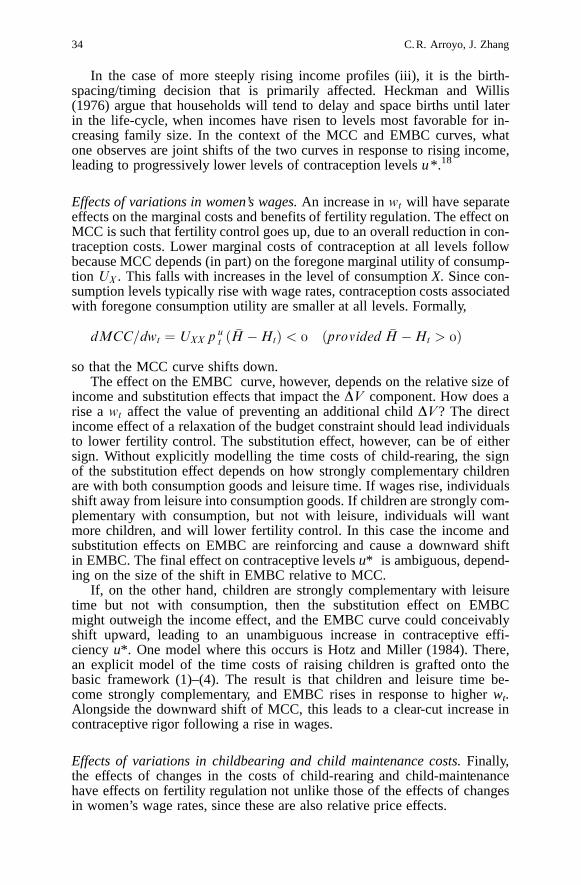
The left- and right-hand-sides of (7) are, respectively, the marginal costs ofcontraception (MCC) and the expected marginal benefits of contraception(EMBC). These are plotted in Fig. 1 over the range ofu. The graph ofUXt p

ut �Uut is drawn as an upward sloping curve taking on positive val-

ues, and this reflects the usual assumptions (see Heckman and Willis 1976,or Leung 1991) thatUX > 0; UXX < 0, and thatUu < 0; Uuu < 0 (i.e., theincrements of contraceptive disutility fall as one increases contraceptivelevels). On the other hand, the graph of the expected marginal benefits ofcontraception is a flat curve inu, whose exact sign and location is deter-mined by the sign and value of

DV �Mt�1; t� 1� � V �Mt; t� 1� ÿ V �Mt � 1; t� 1�; �8�which is the capitalized value (att+1) of preventing a birth att, given par-ity Mt. In all the models considered here, variations in the contraceptive


u–

βπb∆V

u∗ u–0

Marginalutility

u (Contraceptive efficiency)

EMBC

MCC = Uxtptu - Uut

Fig. 1. Marginal costs of contraception, expected marginal benefits of contraception, and opti-mal contraceptive efficiency

decision (or the birth decision, in the case where fertility control is perfect)are due to shifts in their respective MCC and EMBC curves. These shiftsgovern the evolution of fertility control over time.11 Via their effect onthese curves, one may analyze the impact of time-variations in exogenousvariables or parameters on the likelihood of a birth. The resulting changesin birth timing and spacing patterns, and completed fertility levels followdirectly.

Equation (8) highlights the principal practical difficulty attendant to cur-rent structural models. With the exception of Newman’s (1988) model, vir-tually no structural fertility model generates closed-form solutions for theEMBC curve as a function of basic variables and parameters. This createssubstantial difficulties not just for arriving at an econometrically estimableversion of the theory, it also makes it difficult to conduct comparative dy-namics cleanly, with respect to the effects of changes in variables of inter-est on birth control and the birth hazard. For this reason, we rely heavilyon the results of Newman (1988) to guide our discussion of comparativedynamics that follows. In addition, as the models nested inside the abovegeneral structure make different structural assumptions, the mapping frombasic variables and parameters to MCC or EMBC will vary somewhat frommodel to model. Where these lead to substantive differences in predictions,we provide some extra discussion.

Effects of variations in family size.The six prototypical models mentionedabove produce different predictions about the response of the birth likeli-hood and contraceptive efficiency to changes in family sizeMt (i.e., par-ity). We now attempt to sort out these apparently conflicting findings.

A key theoretical result that frequently appears in the literature is con-cavity of the value functionV in family sizeMt. Under reasonable condi-tions, it has been shown that when the underlying period utility functionUis concave inMt, the value functionV will also be concave inMt.

12 Thisimplies thatDV in (8) will increase with parity, as the negative ofDV willdecrease withMt. So as the number of births increase, the EMBC curveshifts up, which tends to raise contraceptive efficiency. The effect of largerMt on the MCC curve, however, is not clear-cut, and its sign depends tosome degree on how strongly children substitute for market goods. Studieswith contraception in the utility function typically assume that the cross-partialUXu � 0. With this, the derivative of the left-hand-side of (7) withrespect toMt is

dMCC=dMt � �UXM ÿUXX pMt � p ut :

Thus, ifUXM=pMt ÿUXX exceeds (is below) zero the MCC curve shifts up(down) as parityMt rises. AsÿUXX is nonnegative, the MCC curve isguaranteed to shift up with risingMt if children are gross complements tomarket goods, that is,UXM > 0. In this case, the tension between the sepa-rate upward shifts of EMBC and MCC confound the final effect of risingMt on the level of contraceptionut. More generally, whenUXM=p

Mt ÿUXX > 0, the final effect on contraceptive efficiency isambig-

uous, depending on the relative size of the shifts of EMBC and MCC.13


The shift of EMBC is large when (i) the discount factorb is large (i.e.,people do not discount future utility so heavily), (ii) the probability of a birthp b is high, and (iii)V is very concave inMt, so that the response ofDV tohigherMt is large (this usually means that the marginal utility of additionalchildren falls quickly). All of these are more plausible for developed econo-mies rather than developing economies.14 The shift of MCC due to increasedfamily size will be smaller and less positive (iv) the lower are the explicitcosts of contraception, and (v) the larger is the utility loss from being ableto consume fewer market goods. These are also more likely to hold in devel-oped societies. The above five considerations are consistent with Newman(1988). Generally then, in developed economies, mothers with larger familieswould tend to have higher contraceptive efficiency levels. In these situations,births will tend to be fewer and more widely-spaced as parity rises. In devel-oping economies, it could go either way.

There are two cases in which contraceptive efficiency increasesunam-biguously with parity. The first is whenUXM=pMt ÿUXX < 0, which isreally a strong form of (v) above. This guarantees that the MCC curve willshift downward, which together with an upward shift in EMBC, will ensurethat the optimalu � will be higher. The other case is when MCC does notshift at all, in which case the concavity ofV in Mt, which is behind the up-ward shift of EMBC, is what drives higher contraceptive efficiency. Quiteimportantly, a positive or negative shift of MCC requires thatp ut not bezero, which is the case in Rosenzweig and Schultz (1985) and Newman(1988), but not in any of the other studies.

For instance, Leung (1991) finds that contraceptive efficiency is alwaysincreasing in parity (despite the assumption that children and market goodsare gross complements) and this result hinges entirely onV being concavein Mt. The omission of explicit contraception costs in the budget con-straint, which Leung argues is not critical to his analysis, is partly responsi-ble for his unambiguous result. Thus, unless one includes the effects onmarginal contraception costs that channel through explicit costs of contra-ception p ut one does not get a decreasing frequency/probability of birthswith parity, nor any threshold effects, which have been detected in somedeveloping economies.15

Effects of variation in elapsed time without a birth.As shown by Newman(1988) the optimal level of contraceptive efficiency decreases with theamount of time that has passed without a birth. In his model, this happensbecause with a fixed family sizeMt; DV ends up being a negative functionof time. The secular decline inDV , in turn, generates a downward drift inthe EMBC curve while the MCC curve is not affected by elapsed timewithout a birth, resulting in a declining time path of optimal contraceptionlevels, ceteris paribus.The intuition is as follows: suppose the EMBCcurve was above the zero level in the preceding period, so that theindividual found it beneficial to prevent a birth then. If the individual waslucky and no birth occurred in the previous period she can relax the controla little in the current period, as the remaining amount of time she faces abirth risk is shorter.16 In effect, the individual finds it optimal to maintainan (almost) fixed “lifetime” hazard of an additional birth, which implies de-creasing contraceptive vigilance as the end of the fertile cycle draws near.


Newman’s result is a sharpening of an earlier conjecture made by Heck-man and Willis (1976) which, in addition to the behavior suggested above,also considered the possibility thatDV is constant over time, so that thebirth hazard remains constant in each period that a birth does not occur, butthe individual’s “lifetime” hazard actually falls over time. In this case, thecontraceptive response is invariant to elapsed time without a birth until theperiodic birth hazard finally results in an “accidental” birth. When this hap-pens the individual will then raise contraceptive efficiency because familysize has increased, but contraceptive efficiency is kept steady until the nextbirth occurs, etc. Newman’s solution, however, rules out this type of behav-ior.

Hotz and Miller (1984) supply an additional reason for why a downwarddrift in DV is likely. If, for a fixed family size, the requisite childrearing timefalls as children age, then as time elapses without a new birth, the capitalizednet benefits of contracepting, captured byDV; will fall naturally. This gener-ally leads to a lowering of contraceptive efficiency levels and a higheruncon-ditional birth hazard in each period. If, however, the individual faces a suffi-ciently large positive risk of infertility even bevore menopause is reached, theconditionalhazard (i.e., the hazard, as of the present timet) of a birth t� jperiods away may not vary positively with elapsed timej. Let q be the prob-ability of becoming permanently sterile in a period. The probability, then, ofremaining fertile forj periods after the last birth is�1ÿ q�j. This is decreas-ing in elapsed timej. Consequently, the chances of a birth occurring att� jwill be smaller the farther awayt� j is from t.

Effects of variations in natural fertility.Newman (1988) shows that an in-crease in the natural probability of a birthp b (i.e., “fecundity”) tends toraise the net birth probabilityp, even though the optimal response to a per-ceived increase inp b is to raise contraceptive levelsut. This can be seen,in a loose sense, in terms of the shifts in the MCC and EMBC curves, asp b is a scale factor for EMBC. An increase inp b would tend to shift theEMBC curve up without affecting the MCC curve. Now there is, however,an additional implicit effect ofp b on EMBC, which happens via the termDV . DV is implicitly a function of natural fertilityp b through future utilityand the future optimal contraceptive levels ofu �t (which depends onp b).Intuitively, however, the effect of higherp b should be to raise futurecontraceptive levels if it raises current contraception levels. But raising fu-ture contraceptive levels is consistent with a rise inDV , rather than a fallin DV. So the indirect effect on EMBC viaDV should only reinforce thedirect effect of a rise inp b.

Since the birth hazardp b (1–ut) rises, however, the implication is thatmore fecund women will have more births, and, because of the birth-spac-ing effect of increases in parity, will tend to cluster their births in the ear-lier years of their fertile cycle. This creates issues of how one handles het-erogeneity in natural fertility levels when one goes about estimating hazardfunctions.

Rosenzweig and Schultz (1985) also find a theoretically positive contra-ceptive response to an increase inp b, although in their framework a dis-tinction is drawn between “permanent” or persistent shocks to natural fertil-ity, and “transitory” ones. They find that the contraceptive response is larg-


er if individuals know that the rise inp b will persist for many periods, andis smaller if individuals are unsure about whether the rise inp b comesfrom the permanent component of natural fertility or the transitory compo-nent. This lack of information further confounds one’s ability to estimatethe size of the effects of heterogeneous fertility levels on the birth hazard.The final effect on the birth hazard of a rise inp b, which would incorpo-rate the optimal contraceptive response to this change, is much more com-plicated than in Newman (1988).

Effects of variations in infant mortality risk.As the probability of an infantdeath,p m), rises, this usually results in a lowernet birth probabilityp, giv-en that morality risks are typically modelled as affecting current birth out-comes only. The effect on net fertility should be the same as the case of afall in the probability of a birth,p b �1ÿ u�. That is, the EMBC curve fallsand contraceptive vigilance is relaxed. This type of response of increasingthe birth hazard in response to higher mortality risk is known ashoarding.

If mortality risks also apply to older children, then lower fertility controlresulting from child replacementmotives may also appear. This type ofbirth hazard effect is distinct from hoarding in that it is a response to a real-ized infant death rather than a response to an increase in the likelihood of adeath. Wolpin (1984) calculates that this effect is small in a sample of Ma-laysian households – there a child death typically causes families to in-crease the odds of a birth, but the increase in the expected number of chil-dren thereafter is only 0.015 children. In a dynamic model of fertility con-trol the reason for this (cf. Newman 1988) is quite intuitive: the responseof the optimal control levelu* is usually small when infant mortality ratesare high since the optimal level ofu* already takes into account the largemortality risks. This effect is more difficult to explain, however, in a non-dynamic context of lifetime family size decisions.

Effects of variations in income.Positive variations in incomeIt can comeeither in the form of (i) an one-time increase in beginning period income,(ii) a permanent increase in the level ofIt for all t, or (iii) keeping permanentincome levels the same, a shift in lifetime income profiles with higher in-comes occurring in later years. The models considered do not generally dis-tinguish between cases (i) and (ii), as the associated behavioral responses arequalitatively the same and differ mostly in size, rather than in sign.

In the case of (i) or (ii) the one-time increase in income generally causesthe MCC curve to shift down and to cause fertility control levels to rise be-cause of negative cross effects with the marginal utility of market goodsUX .17 The effect on EMBC, however, is not clear-cut and depends on param-eters. Together with the shift of the MCC curve this results in an ambiguousoutcome on the level of contraceptive efficiencyu* and the potential forthreshold effects. In cases when the discount factor is large, the net birth prob-ability p b is high, or childrearing costs are high, etc., most of the models pre-dict a negative effect on EMBC also (Newman 1988; Leung 1991; and Pro-position 3 in Hotz and Miller 1984). In developed economies where this effectis expected to be large relative to the shift in MCC, the overall effect is a low-ering of fertility control levels, implying larger expected family sizes in devel-oped economies,ceteris paribus.


In the case of more steeply rising income profiles (iii), it is the birth-spacing/timing decision that is primarily affected. Heckman and Willis(1976) argue that households will tend to delay and space births until laterin the life-cycle, when incomes have risen to levels most favorable for in-creasing family size. In the context of the MCC and EMBC curves, whatone observes are joint shifts of the two curves in response to rising income,leading to progressively lower levels of contraception levelsu*.18

Effects of variations in women’s wages.An increase inwt will have separateeffects on the marginal costs and benefits of fertility regulation. The effect onMCC is such that fertility control goes up, due to an overall reduction in con-traception costs. Lower marginal costs of contraception at all levels followbecause MCC depends (in part) on the foregone marginal utility of consump-tion UX . This falls with increases in the level of consumptionX. Since con-sumption levels typically rise with wage rates, contraception costs associatedwith foregone consumption utility are smaller at all levels. Formally,

dMCC=dwt � UXX p ut � �H ÿHt� < 0 �provided �H ÿHt > 0�so that the MCC curve shifts down.

The effect on the EMBC curve, however, depends on the relative size ofincome and substitution effects that impact theDV component. How does arise awt affect the value of preventing an additional childDV? The directincome effect of a relaxation of the budget constraint should lead individualsto lower fertility control. The substitution effect, however, can be of eithersign. Without explicitly modelling the time costs of child-rearing, the signof the substitution effect depends on how strongly complementary childrenare with both consumption goods and leisure time. If wages rise, individualsshift away from leisure into consumption goods. If children are strongly com-plementary with consumption, but not with leisure, individuals will wantmore children, and will lower fertility control. In this case the income andsubstitution effects on EMBC are reinforcing and cause a downward shiftin EMBC. The final effect on contraceptive levelsu* is ambiguous, depend-ing on the size of the shift in EMBC relative to MCC.

If, on the other hand, children are strongly complementary with leisuretime but not with consumption, then the substitution effect on EMBCmight outweigh the income effect, and the EMBC curve could conceivablyshift upward, leading to an unambiguous increase in contraceptive effi-ciencyu*. One model where this occurs is Hotz and Miller (1984). There,an explicit model of the time costs of raising children is grafted onto thebasic framework (1)–(4). The result is that children and leisure time be-come strongly complementary, and EMBC rises in response to higherwt.Alongside the downward shift of MCC, this leads to a clear-cut increase incontraceptive rigor following a rise in wages.

Effects of variations in childbearing and child maintenance costs.Finally,the effects of changes in the costs of child-rearing and child-maintenancehave effects on fertility regulation not unlike those of the effects of changesin women’s wage rates, since these are also relative price effects.


After the first child, a rise inpMt should generally lead to an upwardshift in MCC as

dMCC=dpMt � UXX p ut Mt > 0 �provided Mt > 0�:Once again, however, the final effect on contraceptive efficiencyu* is gener-ally ambiguous, as generallyDV rises in response to higherpMt . (Usually,higher maintenance costs of a larger family size not only have negative in-come effects on household income, they usually also have negative substitu-tion effects on the number of children born.) The rise inDV counters the ef-fect of the shift in MCC.

2.3 Vijverberg’s (1984) model

Before turning to estimation issues, we pause to examine Vijverberg’s(1984) model, which is a legitimate dynamic structural model, but onewhich does not quite fit the above general framework. Vijverberg sets up acontinuous-time counterpart to our general model, but in his view the deci-sion on whether to have a birth in a period consists of two separate deci-sions: (i) how many children to have in the life-cycle, and (ii) given a cho-sen family size, how should births be spread out over the life-cycle, takinginto account child maintenance costs, labor-market opportunities, and theindividual’s demand for leisure.

His model has some distinctive and interesting features, particularly inthe way the individual’s maximization is set up. Vijverberg divides up thelife-cycle of an individual into time periods or intervals. The first set of in-tervals are simply the birth intervals, that is intervalt � 0 is the time inter-val from marriage to the first birth, intervalt � 1 is the time interval be-tween the first and second birth, etc. Once desired lifetime family sizeI(assumed exogenous in Vijverberg’s analysis) is attained, the relevant timeintervals are no longer the birth intervals (there are no more). Rather, thesebecome the amount of time it takes to “wean away” children. For instance,the �I � 1�st period is the interval between the last child’s arrival and theweaning away of the first child, the�I � 2�nd interval is the period be-tween the weaning of the first child and the weaning of the second, and soon. There is, finally, a last period, which starts at the point at which theIthchild is weaned away, and ends with the end of the conjugal relationship.

Under Vijverberg’s theoretical specification, the individual is now imag-ined to maximize in stages. First, taking asgiven and known the “switch-points” (i.e., the demarcation points between time intervals as definedabove) the individual maximizes expected discounted utility inside each in-terval and adds these up to get a life-cycle utility numberLU � that ismaximal, conditional on the known switchpoints. Next, the individual var-ies the switchpoints (which, givenI, number 2I+1) and selects that combi-nation which maximizesLU �. Vijverberg then suggests that a further max-imization “stage” is possible in which the individual maximizes the valueof LU � by varying completed family sizeI.

Like Hotz and Miller (1984) Vijverberg examines the relationship betweenfertility variates and the time-allocation and labor supply decisions of thehousehold. The key element of his empirical model is a “switchpoint equa-


tion”, which guides the decision to accelerate or delay a birth. While certainlyinteresting, the derivation of this equation and the signs of its parameters arefairly involved. We omit this discussion so that we can focus on his empiricalfindings.

Though his sample did not have a large proportion of women with mul-tiple births, Vijverberg nonetheless found that higher wages tend to causeindividuals to delay births, as leisure time and children appear to be com-plementary. Several other predictions of his model were also confirmed:women appear to choose between a career and raising children, higherchild maintenance costs discourage births, higher (permanent) husband’s in-come seems to encourage earlier births, and (contrary to Heckman andWillis’ findings) a rising income profile for women (reflected in higherpre-dictedfuture wages) tends to also cause earlier births!

2.4 Direct estimation of structural parameters

We now look at attempts and suggested methods for estimating the structur-al parameters of a dynamic programming model like (1)– (4). The bases forestimation are either or both of the value function (6) or the optimal policyfunction (7). Because tractable closed-form solutions for (6) or (7) are un-available, most approaches to estimation require augmenting maximum-likelihood procedures with numerical solution of the dynamic program.

Continuous-valued choice variables.Though not exactly tractable, New-man’s (1988) fertility model possesses a closed-form solution for the opti-mal policy and value functions. An earlier paper, Newman and McCul-lough (1984), did in fact estimate a similar-looking model using hazardanalysis methods as described in Sect. 3 below. However, as pointed out inNewman (1988), the Newman-McCullough estimation was not fully struc-tural, since it did not use the form of the hazard function with the optimalcontraceptive policy inserted. A more thorough application of hazard-rateestimation to Newman’s unrestricted model, is not straightforward, and hasyet to be worked out.

Newman’s (1988) model is one in which the choice variable, contracep-tive efficiency, is allowed to vary continuously over an interval. (In addi-tion, his model is set up in continuous rather than discrete time.) In thecontext of time-series models, some recent methods have been developedfor the structural estimation of dynamic programming problems in whichthe choice variables are continuous (see Taylor and Uhlig 1990; Smith1992). These new methods, however, are suitable for: (i) time-series ratherthan panel or cross-sectional data, and (ii) discrete-time, rather thancontinuous-time equations. Bridging the gap between these new methodsand the Newman model may be a fruitful area for future exploration. More-over, with respect to (ii), one advantage is that the new estimation methodsdo not require closed-form solutions, so that abandoning the continuous-time formulation of Newman (1988) may preclude a closed-form solutionfor (6) or (7) but will not compromise estimation.

Discrete choice models.In the realm of models of discrete fertility choice,Rosenzweig and Schultz (1985) is an early model featuring a dynamic struc-


ture a la (1)–(4). However in estimating the model they apply a time-aver-aging procedure that renders the estimating model nondynamic. Moreover,they also do not solve the dynamic program, numerically or analytically, orobtain structural estimates of the parameters of the value function (6) or theoptimal policy function (7). Hotz and Miller (1988) assume linear approxima-tions to the true optimal policy functions derived in Hotz and Miller (1984).Since it is difficult to map back directly from the fitted linear coefficients tothe original structural parameters, their approach is essentially of the reduced-form variety, and is discussed in Sect. 3 below.

Thus far Vijverberg (1984), Wolpin (1984), and, more recently, Hotzand Miller (1993) are the only studies known to us which estimate structur-al parameters of a dynamic model. Wolpin (1984) appears to be the precur-sor in the fertility literature of the new breed of estimable dynamic structur-al models. These, by necessity, combine numerical solution of the dynamicprogram with maximum likelihood estimation of the structural parameters.It is particularly instructive to examine his approach. Wolpin attempts esti-mation of a parameter vector consisting of the utility function parameters,the (assumed) fixed prices of a new birth and consumption, the time dis-count factor, and other parameters of the optimal policy (7). Call this pa-rameter vectora.

Estimation is based on the following decision rule: letV �Mt; t� be thevalue function for the individual’s utility from periodt onward, given thecurrent value of the stateM (in this case, the stock of children). Letht be arandom shock to preferences now allowed to vary witht, and letPt be theprobability at t that an infant will survive into the next period. Under thefunctional form ofU assumed by Wolpin (see Table 1), the decision to adda child or not19 can be shown to depend upon the function:

Jt � Et �V �Mt � 1; t� 1� ÿ V �Mt; t� 1�� Pt ht� ÿEt �DV �Mt�1; t� 1�� Pt ht; �9�

whereEt DV �Mt�1; t� 1� denotes the capitalized value (att+1) of pre-venting a birth att.20 The second term on the right-hand side is the ex-pected change in utility due to any preference shocks for more children.The optimal decision rule for births is therefore:

N �t� 1 iff Jt > 0� 0 iff Jt � 0:

��10�

Optimal birthsN�t thus depend on the value of the functionJt, which inturn depends on the parameters of the unknown value functionsV ��; t� 1�, the parameters of the conditional distribution function thatindividuals use to calculate the conditional expectationEt, the survivalprobabilityPt, and the preference shockht. Inspection of (9) and (10) re-veals that the model follows a classic probit structure, except that one lacksa closed-form expression forEt �DV �Mt�1; t� 1�� in terms of a. Withsome additional assumptions, however, Wolpin demonstrates that this mod-el is still estimable.


Consider (9). Wolpin argues that there is always a unique value ofht,denoting this critical valueh �t , for which the indicator functionJt will bezero. This value is just

h �t � Et �DV �Mt�1; t� 1��=Pt: �11�Assume that individuals know the random shockht at the time of the cur-rent period fertility decision, but the analyst does not ever observeht. Theanalyst cannot then observeJt directly. Current births’N�t , however, areobservable. To proceed Wolpin makes the classical probit assumption thath�t is a normally distributed random variable. Then the probability that theindividual chooses a birth in periodt (conditional onMt� is

Pr �Nt � 1jMt� � 1ÿU �h�t =r�; �12�wherer is the standard error ofh�t andU �x� is the value atx of the standardnormal cumulative density function. Analogously, the conditional probabilityof no birth att is

Pr �Nt � 0jMt� � U �h�t =r�: �13�Let X be the set of time periods where there is a birth, andXc its comple-ment.For individual i, the likelihoodLi of any particular birth pattern is

Li �Yt2X

Pr �Nt � 1jMt�Yt2Xc

Pr �Nt � 0jMt�; �14�

where it is understood thatX; X c; Nt; Mt; and h�t all depend oni, and

thatLi, in general, is a function of parametersa via h�t . Given a sample ofI individuals, the sample likelihood is

L �YIi�1

Li; �15�

which is maximized with respect toa.This the first part of the estimation methodology; the critical second

component of the methodology is the numerical solution of the dynamicprogramming problem. This is where the main computational issues asso-ciated with structural models generally arise.21 Maximizing L involves eval-uatingh�t , which requires, by (11), evaluation of the conditional expectationEt V �Mt�1; t� 1� at Mt�1 �Mt � 1 and Mt�1 �Mt. Let et�1 be nextperiod’s errors22 and f �et�1jMt� their conditional density. The conditionalexpectation att of V �Mt�1; t� 1� is

Et V �Mt�1; t� 1� �Ze

V �Mt�1; t� 1� f �et�1jMt� det�1: �16�

On the face of it, given the current stateMt and a functional form forf ,only one integration appears in (16), and the problem seems easy. But with


no closed-form solution for the optimal fertility policy, the form ofV �Mt�1; t� 1� is not knownfor any of the realizations ofet�1. Indeed,one must solve the entire dynamic program, which at the time requiredbackward solution from periodT, following Bellman’s recursion:

Et V �Mt�1; t� 1� � Et fmax �U ��; Mt� � bEt�1 V �Mt�2; t� 2��g� Et fmax �U ��; Mt� � bEt�1 fmax U ��; Mt�1�� bEt�2 �V �Mt�3; t� 3��g�g �17�

and so on untilt+j=T.To illustrate the computational complexity involved, consider the fol-

lowing specialization of (17). Suppose that in (17)T � t� 3. Evaluating Et�2 �V �Mt�3; t� 3�� is trivial and involves no integration becausein the last period V �Mt�3; t� 3� � U ��; Mt�3�. To evaluateEt�1 �V �Mt�2; t� 2��, however, requires a nontrivial maximization whichinvolves an integration for each value of the stateMt�2. If the state variablecan take onG �Mt�2� � Gt�2 different values, one has to calculateGt�2 in-tegrals. This done, one can take a step backward and solve forEt V �Mt�1; t� 1�. But this requires the calculation ofGt�1 integrals, onefor each possible value of the stateMt�1. In total, solving this 3 period prob-lem requiredG � Gt�1 � Gt�2 integrations.

Now imagine an extremely simple life-cycle problem whereT=21 peri-ods, and that the state vectorMt consists solely of a family size variable.23

Conditional on today’s stateMt, next period’s stateMt�1 can assume twodifferent values,Mt or Mt � 1. This implies a total number of (21–1)×2=40 integrations that must be calculated to solve for the value ofEt V �Mt � 1; t� 1� in the first line of (9). In addition, one also needs val-ues forEt V �Mt; t� 1�, i.e., the expected value function without an extrachild. This implies another 40 integrations. In total, 80 integrations areneeded to solve the dynamic programof a single individualfor a single valueof h�t in (11).

Suppose one has a sample of 100 individuals. This implies that 8000 in-tegrations must be performed in order to evaluate the value of the likeli-hoodL at the initial setting of the parametersa. But maximizingL numeri-cally requires iterating on the value ofa. At each step, i.e., at each newtrial value for a, one must perform 8000 integrations to get a new likeli-hood valueL, so that convergence in 10 iterations implies 80,000 integra-tions. Clearly, even for a very unrealistic model, the computational burdencan be quite formidable.24 These computational demands go up exponen-tially as one increases the dimensionality of the state vectorMt, the num-ber of time periods, the sample size, the dimensionality of the parameterspace, or the number of times one must obtain estimates ofa, say for pol-icy experiments. This is essentially Bellman’s “curse of dimensionality.”

Recent advances in computational methods for discrete-choice models.From the preceding sections it is evident that the principal trade-off in-volved in structural estimation is that of computational simplicity vs. real-ism of the model. This trade-off exists because tractable closed-form valuefunctions or optimal policy functions are unavailable for many interesting


dynamic discrete- choice models. This requires numerical solutions of thedynamic program instead, which leaves one open to the curse of dimen-sionality. Some progress around this problem has been made, and we exam-ine several recent proposals that we view as critical for this effort.

The first of the methodologies below relies on simplifying the calcula-tion of the conditional expectation of the conditional expectationEt V �Mt�1; t� 1�, which appears in the value function recursion (6) or(17). Keane and Wolpin (1994) refer to this as the “EMAX” function, sincewith k=1, ...,K alternative choices one can always write

Et V �Mt�1; t� 1� � Et maxk

Vk �Mt�1; t� 1�: �18�

Herek � 1; :::; K indexes the discrete-valued and mutually exclusive alter-natives the individual chooses from. (In Wolpin’s model above,k takes twovalues:k=0 if the individual chooses not to have a child andk=1 other-wise.)Vk �Mt�1; t� 1� is the value of remaining lifetime utility as oft+1,assuming the individual chooses alternativek at time t, and behaves opti-mally thereafter. (In our version of Wolpin’s model,Vk(Mt+1; t+1)=V(Mt+k; t+1).) Keane and Wolpin (1994) call thesek functions thealterna-tive-specific value functions.These functions satisfy

Vk�Mt�1; t�1��Uk��;Mt�1��bEt�1V�Mt�2; t�2�; k�1; . . .;K : �19�The first (and perhaps most well-known) of the solution methodologies for(19) is Rust (1987). Rust achieved computational simplifications of theEMAX function at the cost of some realism by assuming that: (i) indivi-duals’ utility functions display additive separability of deterministic and sto-chastic components, (ii) given the current level of observable state vari-ables, the stochastic components are serially independent, (iii) the stochas-tic components have a multivariate extreme value distribution. These given,Rust’s two key results were: (i) the EMAX function has a closed-form solu-tion, and (ii) the choice probabilities Pr [k|Mt] are multinomial logit. Asnoted in Keane and Wolpin (1994), these results together allow the analystto avoid costly numerical integrations in solving the dynamic program, andin performing the likelihood estimation.

These assumptions were quite restrictive and ruled out more generalmodels in which the errors display serial correlation or do not follow theextreme value distribution. Since then, several methods have been proposedto relax these restrictions. Rust (1994), in particular, reviews available solu-tion methodologies for the EMAX function in the (realistic) case when theunderlying random process is Markovian. For Markovian processes, theseinclude the method of successive approximations, policy iteration methods,or minimum weighted residual methods. He then lays out a general estima-tion theory for estimates based on these approaches.

Rust also surveys recent results that have been obtained for more generalunderlying random processes. For these, Monte Carlo integration is the natur-al solution method, but it can be very computationally intensive. To lowercomputational costs Keane and Wolpin (1994) and Geweke, Slonim, and Zar-kin (1992) propose combining Monte Carlo integration with interpolations/approximations of the value function (6) or the optimal policy function (7).


Keane and Wolpin (1994) rely on the value function recursion (6) or (19)as a basis for estimation, and try to find a form for the EMAX function of therecursion that can be computed more easily,a la Rust (1987). However, in-stead of deriving an exact form for EMAX, Keane and Wolpin propose ap-proximating functions which are arbitrarily close to the true EMAX functionEtV(Mt+1; t+1). The idea is as follows: (i) first solve the dynamic programbackwards by simulation methods for a reasonably-sized subset of statepoints f ~MtgTt�1; (ii) next, using the simulated values of the value functionV, fit by regression methods an approximating function to the EMAX func-tion, (iii) use the fitted approximation function to interpolate for EMAX val-ues on the remaining state points, (iv) having calculated all the relevantEMAX values, calculate the value of likelihood function at a prespecified val-ue ofa. Then iterate (i)–(iv) ona until the value of the likelihood function isat a maximum.

The general form of the approximating function proposed by Keane andWolpin is

EMAX �Mt; t� �MAXE �Mt; t� � g �MAXE �Mt; t� ÿ �Vk� ; �20�

where MAXE(Mt, t )=maxk Vk, Vk=EtVk(Mt+1; t+1). The differenceMAXE(Mt, t)–Vk insideg(·) is understood here to be ak-vector. The func-tion g is a mapping fromRk to R++, that is, g is real-valued and alwayspositive. The intuition for this form is that the difference beween EMAXand MAXE, which is always positive, will depend on how far apart are theexpectedVk’s from each other, and this distance is captured by the differ-ence MAXE(Mt, t )–Vk. By increasing the number of state space pointsused (relative to the size of the state space) in estimating the interpolatingfunction, one can get arbitrarily good approximations to EMAX.

In Monte Carlo experiments, Keane and Wolpin (1994) find that the fol-lowing form of g worked well:

EMAX �Mt; t� ÿMAXE �Mt; t� � d0 �XKj�1

d1j �MAXEÿ �Vj�

�XKj�1

d2j �MAXEÿ �Vj�1=2 �21�

By simulating the dynamic program at the subset of state pointsf ~MtgTt�1one gets values for both MAXE andVj, as well as EMAX(Mt, t). Thesevalues become the data for estimatingd0, d1j, d2j in (21) by linear regres-sion methods. The fitted version of (21) serves as the interpolating functionfor calculating EMAX(Mt, t) at the remaining state points. The computa-tional gain is that it is much easier to evaluate MAXE or any of theVk’sfor the remaining state space points than it is to calculate EMAX.

Geweke et al. also propose an estimation-interpolation procedure that isvery similar in spirit to that of Keane and Wolpin. The main difference isthat, in this case, the authors work with approximations to the optimal pol-icy function rather than the value functionV. In the Wolpin (1984) model,


the optimal policy function is the step function (10) which depends on theunknown functionJt=Et [V(Mt+1; t+1)–V(Mt; t+1)]+Ptht. In the context ofthat example, Geweke et al. propose approximatingJt by the translated lo-gistic of a polynomial-in-Mt:

~Jt � exp �r p �Mt�0 d�=�1� exp �r p �Mt�0 d�� ÿ 12; �22�

where r p(Mt) is a vector of variables of the formQpi�1 (Mit )

p so that(r p(Mt)'d) is a pth-order polynomial function in the stateMt, with coeffi-cientsd. They show that this approximation can be made arbitrarily goodby increasing the polynomial orderp. To estimated, the authors suggestmaximum likelihood estimation of the logit model

Pr �Nt � 1jM ÿ t� � exp �r p �Mt�0 d�=�1� exp �r p �Mt�0 d�� 23�

based onR simulations offMtgTt�1 and S possible values of the choicevariable. Estimatesc can now be used to construct the approximate deci-sion ruleJ

Jt � exp �r p �Mt�0d�=�1� exp �r p �Mt�0d�� ÿ 12: �24�

Using this decision rule in place of the functionJt (evaluation of which re-quires numerical integration) greatly facilitates further simulations ofMt, aswell as subsequent calculations of the values of the choice variables thatsolve the dynamic program.

Rust (1995) proposes a more promising alternative to Keane-Wolpinwhich is based on a random Bellman operator. His approach is appealingin that it avoids the need for interpolation and repeated simulation, and infact breaks the exponential relationship between computation time and di-mensionality of the state variable.

Perhaps even more promising is the simulation estimator of Hotz et al.(1994), a technique which has the added advantage of being applicable tomore general random processes than Markovian ones. The key discovery ofHotz et al. was that under fairly general conditions, one can “invert” non-parametric estimates of conditional choice probabilities (i.e., the densitiesf (et+1|Mt) in (16)) to get consistent estimates of the value function orEMAX function in a normalizedform. This “nonparametrically estimated”normalized value function can then be used to calculate consistent esti-mates of the optimal decision rule or policy. The estimated decision rule,along with the data on the model variables and the conditional probabilitiesf, can be combined together in a simulation to trace out a “simulated” nor-malized value function. Estimation of the parameter vectora is finally doneby choosinga to minimize the distance between points on the simulatedvalue function and the “nonparametrically estimated” value function. SeeRust (1994) for a more detailed review of this new technique.


Empirical results.With regard to the empirical findings on fertility behavi-or arising from structural models, we review the results in Wolpin (1984),as this is more or less a representative fertility model. Other models havevery unique features and are interesting in their own right, but for spaceconsiderations are only referenced here. For instance, Vijverberg (1984) hasa labor-supply and time-allocation decision in addition to the fertilitychoice. Hotz and Miller (1993) study a model with imperfect fertility con-trol by contraception, but with perfect fertility control by irreversible sterili-zation. Necessarily, their results differ.

Wolpin applied his estimation strategy to a 188-household subsample ofhouseholds in the 1976 Malaysian Family Life Survey, which contains a ret-rospective life history for each household, with birth, infant mortality, andhousehold income. Wolpin then matched these up with Malaysian state-specific survival rates. For his application, Wolpin set the number of time per-iods to 20, each period being an 18-month interval. Time period 1 was set tothe onset of individual’s fertile cycle (age 15 or marriage, whichever camefirst), and at the last decision period (t=20) the fertile cycle was assumedto end, with individuals assumed to live for 10 periods (15 years) thereafter.

After testing for and finding no strong evidence of unobservable in-dividual heterogeneity at work, Wolpin estimated the parameters of hisquadratic utility function (see Table 1) and the parameters of its budgetconstraint (consisting of cost parameters for child maintenance costs, andparameters for the cost of new births). Point estimates of the utility func-tion parameters were reasonable – at point estimates marginal utility waspositive and diminishing in family size and in the consumption good, andtime preference was about 0.09 per annum. A model check using a likeli-hood ratio test revealed a significant enough difference between his mod-el’s results and those from a model of random (Bernoulli) births. So theWolpin structure explained more than by pure chance.

Interestingly, Wolpin found that children and consumption goods tended tobe gross substitutes in utility. The higher the mother’s education levels, how-ever, the lower was the utility of additional children. With respect to the costfunction parameters, Wolpin found large costs of new births, which followeda decreasing then increasing pattern over the life-cycle. Maintenance costs,however, appeared to be small and reasonable. With respect to income, a risein husband’s current income tended to have a large positive effect on the num-ber of births, with larger income elasticities of a birth appearing at the higherincome extremes. The expected number of children ever born did not varymuch with the realization of an infant death, so estimated replacement behav-ior was extremely small (an infant death inducing a rise in children ever bornby an average of only 0.015). However, the response to higher probabilities ofinfant mortality risks was not small. Indeed, Wolpin found that a fall in themortaility probability by only 0.05 percentage points reduced the numberof children ever born by about one-quarter.

Regarding the implied comparative dynamics, Wolpin found thatindividuals who over time expected rising incomes and falling mortalityrisks tended to delay births. This finding is consistent with predictions ofHeckman and Willis (1976). Further, a lowering of mortality risks gener-ated a tendency to cluster births in early periods of life, while a rising sur-vival probability profile tended to delay childbearing.


In short, Wolpin found: (i) small income effects; (ii) large and negativeeducation effects; (iii) very small positive replacement effects, and a non-monotonic relationship between current birth probabilities and family size;(iv) no unobservable heterogeneity among individuals, and (v) a negativeeffect on fertility of higher mortality risk.

Of interest is a comparison of these five results against results thatcould be obtained from a typical static reduced-form model. As a final ex-ercise, Wolpin did a probit estimation of the birth likelihood taking familysize, current and expected income, current and expected infant survivalprobabilities, and mother’s schooling as regressors. The comparative-staticresults were as follows. Like structural estimates, the fitted probit regres-sions implied: (i) negligible income effects on birth probabilities, and (ii)negative education effects. Unlike the structural estimates, however, thenonstructural probit model produced (iii) an insignificant or positive effectof family size on current birth decisions, the positive effect suggesting (iv)potentially unobserved heterogeneity; and (v) a positive effect on fertilityof higher mortality risk. Evidently, the two approaches see the relationshipbetween births and fertility variates differently. It remains an open questionas to which approach gives the more believable results.

The empirical properties of Wolpin’s (1984) model indicate that a rela-tively simple version of the dynamic programming model (1)–(6) is cap-able of replicating some fairly complex properties of birth history data.While the computational complexity of the estimation strategy is an issue,it is fair to ask how complex a comparable non-structural alternative wouldhave to be to replicate all the possible birth patterns in the data. Wolpin fig-ured that, to do this, a comparable nonstructural econometric model wouldrequire the estimation of around 400 parameters, instead of the 13 of hisstructural model. Computationally, such a model would also be fairly de-manding. Given the recent advancements in the computation of structuralestimates for even richer models, there appears to be an expanding empiri-cal role for structural dynamic models. Nonetheless, dynamic reduced-formmodels continue to be useful and are usually more tractable alternatives.We now turn to these models.

3. Reduced-form models

In this section we consider the class of dynamic reduced-form fertility mod-els, with focus on research by economists. As mentioned in the introduc-tion, reduced-form models may have a basis in some dynamic program-ming problems but do not rely heavily on that structure for the specifica-tion of estimating equations. Specification of the estimating relationships,including stochastic elements, is often made in conformity with some tract-able econometric framework; these models typically use the underlying the-ory to posit variables and possible error structures.

In most of these studies the main variable of interest is the birth likeli-hood. When this variable is regarded as continuously-varying, practicallyall reduced-form dynamic fertility models adopt a hazard-rate approach toestimation. When the birth probability (and the contraceptive efficiency)


takes on discrete (dichotomous) values, the empirical methodology of Hotzand Miller (1988) is a viable alternative.

3.1 Hazard-rate analysis (Heckman and Walker, etc.)

Formulation and estimation.Hazard-rate analysis, also often called dura-tion or event history analsys, is proving useful in a variety of problems ineconomics.25 Indeed, most economic research on timing and spacing ofbirths has used the hazard approach. Specifically, this framework is fol-lowed in Newman (1983); Heckman et al. (1985); Newman and McCul-lough (1984); Heckman and Walker (1987, 1989, 1990a,b, 1991); and Da-vid and Mroz (1989). In this approach, women are assumed to be continu-ously subject to the risk of a birth. The risk is given by the hazard rate, de-fined as the conditional probability of a birth at timet given no birth imme-diately beforet. The hazard rate may vary randomly across the population(referred to asheterogeneity) and may vary over time spent in a birth inter-val (referred to asduration dependence).

In a series of papers, Heckman and Walker present semiparametric multi-spell fertility models. Their models are first discussed here because they aremore general than others. It will become clear that models used in Newman(1983), Heckman et al. (1985), and Newman and McCullough (1984) can beconsidered as special cases. Following the notation of Heckman and Walker, awoman’s birth history is assumed to evolve in the following way. The womanbecomes at risk for the first birth at calendar times=0. Define a finite-statecontinuous-time birth process {Y(s), s>0}, Y(s) ∈ C, where the set of possi-ble attained birth states (parities) is finite (C={0, 1, 2, . . ., c}, c<?). An ele-ment ofC defines the number of children born.Y(s) is parity attained ats.Transitions occur on or afters=0. Child mortality is not considered.

The basic component for multistage duration models is the conditionalhazard. DefineH (s) as the relevant conditioning set at times, which mayinclude anticipitations about the future formed at times and relevant pastinformation up to times (previous birth intervals, etc.).

Define the potential durations byT1, . . . ; Tc. If a woman becomes atrisk for the jth birth at times (j–1), the conditional hazard at durationtj isdefined to be

hj �tjjH �s �j ÿ 1� � tj�� : �25�Assuming thatTj is absolutely continuous givenH, we may integrate (25)to find the survivor function

S �tjjH �s �j ÿ 1� � tj�� exp ÿZtj0

hj �ujH �s �j ÿ 1� � u�� du24 35 : �26�

The assumption of absolute continuity rules out conditioning on variablesthat perfectly predict the fertility outcome.

A woman at risk for a first birth ats=0 continues childless a randomlength of time governed by the survivor function


Pr �T1> t1jH �s �0��t1�� exp ÿZt10

hj�ujH�s�kÿ1��u�� du24 35: �27�

At time s (1), the woman conceives and moves to the stateY(s)=1. In thegeneral case,Y(s)=k–1 for s (k–1)≤s<s (k) and Tk=s (k)–s (k–1) is gov-erned by the conditional survivor function

Pr �Tk> tkjH�s�kÿ1��tk��exp ÿZtk0

hk�ujH�s�kÿ1��u�� du24 35: �28�

The conditional density function of durationSk= tk is given by the productof the hazard and survivor functions

g�tkjH�s�kÿ1��tk�� hk�tkjH�s�kÿ1��tk��S�tkjH�s�kÿ1��tk�� : �29�Modelling unobserved heterogeneity (e.g., fecundity) is necessary be-

cause it is virtually impossible to measure all important covariates appropri-ately.26 Recent work shows the importance of controlling for heterogeneityin hazard models (Heckman and Walker 1985; Heckman et al. 1985; Trus-sell and Richards 1985; Manton et al. 1986; Struthers and Kalbfleisch1986; Sturm and Zhang 1993; Zhang and Sturm 1994). Heckman andWalker distinguish two types of unobservables: (i) those that are known tothe woman being studied but unknown to the researcher, and (ii) those thatare not known to both the woman and the researcher. They point out thatthe latter type of heterogeneity can produce dynamics of its own if theagents being studied learn about their unobservables over the life cycle,and provides the rationale for including lagged birth intervals as explana-tory variables as in Rodriguez et al. (1984).

Heckman and Walker point out that the study of heterogeneity in multi-stage duration models is in its infancy. The few studies that include unob-served heterogeneity consider the first type and universally assume the het-erogeneity can be represented by a scalar random variableh which is time-invariant with distributionM (h). Densities are now defined conditional onH (s) andh:

g �tkjH�s�kÿ 1� � tk�; h� � hk�tkjH�s�kÿ 1� � tk�; h�� S�tkjH�s�kÿ 1� � tk�; h�� : �30�

The conditional density ofT1, . . . ; Tc givenH�s�0� �Pci�1 ti� is then

g t1; . . . ; tcjH s�0��Xci�1

ti

!" #�Zh

Yck�1

g �tkjH�s�kÿ 1� � tk�; h�dM �h��31�

whereh is the support ofh, i.e., its domain of definition.


In their empirical specification, Heckman and Walker approximate thejth conditional hazard using the following functional form

hj�tjjH�s�j ÿ 1� � tj�; h� � exp c0j �XKjk�1

ckjtkkjj ÿ 1kkj

!� Z bj � fjh

" #;

�32�

whereZ includes all observed regressors possibly including durations fromprevious spells and spline functions of current durations. Parity dependenceis incorporated by allowing coefficients to bear parity-specific subscripts.

An important feature of hazard specification (32) is that it encompassesa variety of widely-used models. Settingbj =0, Kj =1, and fj =0, (32)specializes to a Weibull model ifk1j =0, to a Gompertz hazard ifk1j =1,and to a quadratic model ifKj =2 andk1j =1 andk2j =2. It becomes an ex-ponential model ifckj=0 for all k. This general framework allows us to uselikelihood ratio tests to choose among many conventional competing speci-fications. Specification (32) also extends previous duration models by al-lowing for general time-varying covariates and by introducing unobservedheterogeneity that is correlated across spells.27 Permitting thefj to vary byparity j allows the scalar unobservable to play a different role in differentspells.

The conventional way to include unobserved heterogeneity is to assumea parametric function forM (h), as in Newman and McCullough (1984).Such procedures have been called into question because of the sensitivityof the estimated parameters to choices of functional forms for the hazardand heterogeneity. Heckman and Singer (1984) show thatM (h) can be esti-mated nonparametrically. However, Trussell and Richards (1985) demon-strate nonrobustness of estimates to choices of functional forms for hazardeven whenM (h) is estimated nonparametrically. These sensitivity resultsare widely cited as “discouraging” evidence on the value of incorporatingunobserved heterogeneity into hazard models. Montgomery and Trussell(1985, p. 30) capture this negative mood in the demographic literature:

This sensitivity to the choice of functional forms of the distribution ofunobservables or of the hazard leaves us profoundly depressed aboutwhere next to proceed. We fear that the advances in statistical techniquehave far outpaced our ability to collect data and our understanding ofthe behavioral and biological processes of interest.

Heckman and Walker (1987) argue that missing from the pessimistic as-sessments of models with unobservables is any discussion of the fit ofalternative models to the data. They demonstrate that, in contrast to the pre-sumption in the demographic literature that preferred alternative models fitthe data equally well, few models can fit the data at all. Because manymodels are non-nested, we confront the problem of non-nested model selec-tion when seeking a “best” model. Heckman and Walker (1990 a, 1991)propose and describe four widely used criteria: (i) the Leamer-Schwarz cri-terion that penalizes likelihood for parametric estimation; (ii) the criterionof picking a model on the basis of coefficient stability across cohorts; (iii)


the effectiveness of fitted micro-models in predicting aggregate time series;and (iv) a criterion widely used by demographers – predicting fertility at-tained (parity) at different ages.

In Heckman and Walker (1987, 1990 a, b, 1991) they estimateM (h) bythe nonparametric maximum likelihood (NPMLE) procedure of Heckmanand Singer (1984). This procedure approximates any distribution functionsof unobservables with a finite mixing distribution, {pi, hi} i = 1, wherepi isthe weight placed onhi. The NPMLE procedure estimates support pointshi, i =1,...,I and the weight placed on the support points

pi; i � 1; :::; I whereXIi�1

pi � 1 !

along with other parametersof the model.

Finally, Heckman and Walker’s empirical framework allows for period-specific stopping behavior. The survivor function for thejth birth is

Sj �tjjH �s �j ÿ 1� � tj�; h� � P�jÿ1�

� �1ÿ P�jÿ1�� exp ÿZtj0

hj �ujH �s �j ÿ 1� � u�; h� du24 35; �33�

whereP(j–1) is the probability that a woman withj–1 children is never atrisk to have thejth birth and thus captures permanent biological or behav-ioral sterility (i.e. a parity-specific mover-stayer mixture distribution).28 Thecontribution to sample likelihood of a woman with fertility historyT1= t1, T2= t2,...,Tk= tk and an incompletek+1 spell of lengthtk+1 is

XIj�1

Ykj�1ÿ @ ln Sj �tjjH �s �j ÿ 1� � tj�; hi�

@tj

� �� Sj �tjjH �s �j ÿ 1� � tj�; hi�

� Sk�1 ��tk�1jH �s �j ÿ 1� � tj�; hi� pi : �34�

A general multistate computer program, CTM, applicable to multistate com-peting risks models much more general than a birth process, is used to esti-mate the model. The details of the computer program are in Yi, Walker,and Honore (1987) and Heckman and Walker (1987).

Other formulations can be seen as special cases of Heckman and Walker’sformulation. Newman and McCulloch (1984) model duration dependence as athree point linear spline and assume a parametric Gamma distribution for un-observed heterogeneity forM (h). Heckman et al. (1985) is almost identical tothe general formulation of Heckman and Walker, except that the former studymodels duration dependence as a quadratic polynomial and the latter uses ageneral Box-Cox transformation. All these studies allow for time-varyingcovariates. Allowing for period-specific stopping behavior is an unique fea-ture of the general Heckman-Walker formulation.

David and Mroz’s (1989) empirical model is similar to the general Heck-man-Walker framework in several aspects. David and Mroz model unob-served heterogeneity and period-specific stopping behavior (called as second-ary sterility) as in Heckman and Walker. However, there are several differ-


ences in specifications. Child mortality is ignored in Heckman and Walker,but is modeled as an independent random censoring of the birth process. Inanother word, they define the duration as the minimum of the waiting timeto a live birth and the waiting time to the death of the youngest child. UnlikeHeckman and Walker, David and Mroz assume a log-logistic function for theconditional hazard. (See Kalbfleisch and Prentice (1980) for a discussion ofthe relation between log-logistic functions and other functions such as Wei-bull.) As a minor difference, David and Mroz allow the weight placed onthe support points (pi, i =1,...,I) to be determined by a multinominal logisticfunction of some observable characteristics.

Empirical results.Table 2 summarizes the empirical results in Newman andMcCullouch (1984), Heckman et al. (1985), David and Mroz (1989), Heck-man and Walker (1990 a, b, 1991), and Tasiran (1995). Newman andMcCullouch estimated their hazard model with Gamma heterogeneity forbirth history up to age 30 for four cohorts of women from ages 30 to 49 atfive-year intervals. It is found that higher female education delays the firstbirth of all birth cohorts and delays subsequent births of all cohorts exceptthe birth cohort 40–44.29 While the education of the male is not (statisti-cally) significant in determining the risk of the first birth, it is important indelaying subsequent births. Women in younger cohorts living in areas withhigher child mortality tend to have the first and subsequent births earlier.The family planning variable is never significant at a conventional level.

Heckman et al. find that some “stylized facts” of the demographic litera-ture are not robust to unobserved heterogeneity. Rodriguez et al. (1984)suggest that age at marriage and/or the entry into parenthood are the crucialdeterminant of life cycle fertility and that variation in completed fertilityacross the population comes primarily from these initial conditions, andthat subsequent childbearing is largely determined by initial events and byprevious birth intervals. Using the Swedish data, Heckman et al. (1985)find that, in models that do not control for heterogeneity, the longer a pre-ceding birth interval the longer the subsequent one, exhibiting the “engineof fertility” phenomenon noted by demographers.

Controlling for heterogeneity, the “well-noted empirical regularity” eithervanishes or reverses in sign. For a sample of married women, it vanishes en-tirely. Furthermore, for all women and controlling for marital status as a cov-ariate, inclusion of heterogeneity produces a “reverse engine of fertility” phe-nomenon: the longer the preceding birth interval the shorter the subsequentone. For the married women sample, the importance of age at marriage onthe spacing of births is considerably reduced in size and statistical signifi-cance. For the sample of all women, controlling for heterogeneity eliminatesthe effect of age at marriage on all but the final birth transition.

Emphasizing the roles of female wages and male income, Heckman andWalker (1990 a, b, 1991) find that female wages delay times to all concep-tions and reduce total conception. This result is shown to be robust to a vari-ety of empirical specifications. Higher male income reduces times to concep-tions (strongest effect for the first birth) and increases total conceptions whenmarital status is not controlled for. The estimated male income effect is weak-er when marital status is included as a separate regressor. Somewhat surpris-ingly, unobserved heterogeneity correlated across spells is not an important


feature of modern Swedish fertility data.30 In all models in which nonzeroduration dependence is permitted, they find positive duration dependence.Their major finding is that a neoclassical model of fertility outperforms demo-graphic models which exclude wage and income variables in terms of severalmodel selection criteria.

As Heckman and Walker point out, the most controversial aspect oftheir study is its use of cohort average wages as proxies for missing microwages. While the use of average wages almost eliminates the possibility ofsimultaneous equation bias in estimating the relation between wages andfertility, it introduces an errors-in-variables problem and a spurious relation-ship between strongly time-trended variables (i.e., wages and fertility).Heckman and Walker demonstrate that the results on female wages andmale income are robust to those considerations.

Heckman and Walker (1989) use estimates of individual fertility dynamicsobtained in Heckman and Walker (1990a,b, 1991) to forecast aggregate an-nual birth rates for each cohort. They examine the ability of microdynamic


Table 2. Empirical results from reduced-form models

Authors (Year) Emphasized(or primary)covariates

Other or additionalcovariates

Dataset

Heckman, Hotz andWalker (1985)

Age at marriage,previous birthintervals

Current spell duration,labor participation,schooling, urban, white-collar, attended univer-sity

1981 SwedishFertility Survey

Heckman and Walker(1990a,b, 1991)

Female wage andmale income

Current spell duration,urban, white-collar,age, time trend, at-tended university,ever-married, unem-ployment rate, policymeasures

1981 SwedishFertility Survey

Tasiran (1995) Female wage, maleincome, femaleschooling, andworking experience

Current spell duration,urban, white, age atunion start, birthcohorts, ever-married

1981 Swedish Fertil-ity Survey, Swedish1984 and 1988Household Marketand Non-MarketActivities, 1985–1988 PSID

Newman andMcCulloch (1984)

Male and femaleyears of schooling

Female’s birth year,child mortality, familyplanning measure

1976 Costa RicaNational FertilitySurvey

David and Mroz (1989) Age of husbandand wife, previouschild’s sex, numberof boys and girlsalive, number ofboys and girls aliveaged 10 or older

Number of priordeaths of boys andgirls before the 3rdmonth, number ofprior deaths of boysand girls aged 3–11months, villagemortality

Rural France datarelating to the mar-riage cohorts of1749–1789

models to account for time series variation in cohort fertility. They find that,for most Swedish women, their estimated models pass some important timeseries specification tests. They also find that their aggregated neoclassical mi-crodynamic models explain the time series better, in the sense of meansquared error of forecast, than do time series regressions.

Building on Heckman and Walker’s work, Tasiran (1995) provides newevidence for the role of female wages and male income in the fertility ofSwedish women. Tasiran modified the macro wage and income series usedby Heckman and Walker, and made use of micro wage and income data inindividual income-tax records from Statistics Sweden. He constructed twocombined macro-micro wage series. For the first combined series, he usedHeckman and Walker’s series for the years 1948–1967 and 1981, and forthe period 1968–1980 the micro wage data derived from income-tax re-cords. For the second combined series he used wages of salespersons andshop assistants for the years 1948–1967 and 1981, and for the period1968–1980 the micro wage data. He also included a variable for women’syears of working experience.

Tasiran reports that the Heckman-Walker results of a negative wage ef-fect and a positive income effect do not hold generally. The sign and statis-tical significance of female wages and male income are sensitive to paritylevel, measurement of wages and income, controlling for unobserved het-erogeneity, inclusion of working experience, and data sets. Tasiran’s mainconclusion is that the effects of female and income are not robust and aremuch weaker than Heckman-Walker indicated. He also finds that years offemale schooling and of working experience significantly delays the firstbirth but have weaker effects on higher births.

In a reply to Tasiran (1995), Walker (1996) criticizes Tasiran’s casualuse of micro wages. Specifically, Walker points out that a more carefulanalysis would have addressed four issues on the use of individual wages.First, he argues that a simple merging of aggregate and micro data is inap-propriate. Second, the issue of wages of nonworking women was not ad-dressed by Tasiran. Third (and most importantly, according to Walker), in-adequate attention was paid to measurement error in individual wages. Fi-nally, exogeneity of wages and selection bias should be addressed.

The main finding of Walker’s thoughtful analysis is that there is sub-stantial measurement error in individual wages in birth years. Controllingfor measurement error by dropping birth year observations, the selection ef-fect appears to be minimal. Estimates from a wage regression (excludingbirth years observations) were then used to backcast female wages before1968 and to fill in wages for nonworking women. As Walker finds,

For the first transition the estimated wage effects are roughly two-thirdsthe magnitude of the effects estimated by aggregate wages. Even in thehigher parities, the estimated wage effects are quantitatively large andstatistically significant. Although the cohort drift which was present inthe estimates obtained from aggregate data is not present, the statisticalsignificance and importance remain. (Walker 1996)


Replying to Walker’s comment, Tasiran (1996) writes

The results in rows 5 of Walker’s Table 3 is an excellent illustration ofthe sensitivity of the estimates of the wage rate effects on fertility andthat the first Heckman and Walker estimates were on the high side.Comparing rows 5 with rows 3, 11 out of 12 estimates in rows 5 areless in absolute value than the corresponding estimates in rows 3 andseveral are substantially lower.

Walker’s analysis of the individual wages certainly highlights the impor-tance of careful and thoughtful work on micro data. His findings also lendsupport for the results of Heckman and Walker obtained by aggregate datain wages. The debate between Walker and Tasiran, however, is valuable, asit illuminates the complicated fertility dynamics in Sweden. The centralproblem is a lack of high quality micro wage data. Given this problem, itis not surprising to find different results when individual wages are con-structed and handled differently. The issue of robustness of results shouldbe dealt with carefully. When magnitude differs across different wage se-ries, Tasiran appears to interpret the results to be sensitive. Walker, on theother hand, believes that as long as statistical significance is preserved, theresults are robust. Interpreted with care, Walker’s new results show that theoriginal Heckman-Walker findings are, to some extent, robust.

We believe that there are still some issues that require further investiga-tion. First, Walker’s analysis shows that there is substantial measurementerror in wages for birth year observations. The question is: why? Tasiran(1996) thinks that the measurement error is mainly in working hours whichhe obtained from Heckman and Walker. Rather than simply deleting birthyears observations (when estimating the wage regression) and thus losinguseful information, a reexamination of the data on earnings and workinghours might be necessary to determine the sources of, and possible reme-dies for, measurement errors in micro wages.

Second, Walker (1996) also used the female wage series for shop assis-tants and found the wage effects were small for younger cohorts. Walkerargues that the inability to recover statistically significant wage effects forthe youngest cohorts stems from the flatter age-profile of wages during aperiod of low wage growth. Specifically, he mentions that the observed de-cline in the wage dispersion during the 1970s reflects the compression aris-ing from the adoption of wage solidarity. If that was the case, how can theuse of aggregate macro wages show statistically significant wage effects inHeckman and Walker? That would be possible if there was more variationin macro wages than in female shop assistant wages. But why should theslow-wage-growthcum flatter-age-profile argument apply to female shopassistants, but not to macro wages? Therefore it appears necessary to inves-tigate whether the age-profile of wages is flatter for shop assistants than forother workers.

David and Mroz (1989) estimate their model using data from rural Francerelating to the marriage cohorts of 1749–1789, a population that is supposedby many demographers to be identified with “natural fertility”, namely, theabsence of parity dependence in age-specific marital fertility rates. Their cen-tral concern is to re-examine this widespread “natural fertility” suppositionwith suitable econometric methods. They obtain strong evidence against the


“natural fertility” characterization of the demographic regime that prevailed inrural France immediately before the Revolution of 1789.

There are clear indications that marital fertility rates were being regu-lated in congruence with the differential valuations placed upon children,according to their gender and age. In particular, controlling for the totalnumbers of young children and old children, the presence of a larger num-ber of young girls leads to a lower hazard rate, but that of a larger numberof young boys has no such effect. A larger number of older children, re-gardless of gender, reduces the hazard rate. They attribute the differentialresponse by age of children to risk aversion and the greater risk of losing ayounger boy to mortality. Village mortality is found to have a positive ef-fect on the hazard, suggesting the presence of hoarding behavior in fertility.They also find strong replacement effects to the deaths of boys (especiallyboys aged two months or above). To the contrary, there is weak evidencethat the death of young girls reduces the hazard rate. They argue that theseresults suggest the endogeneity of child mortality.

3.2 Quasi-maximum likelihood estimates of linear decision rules

When the contraceptive efficiency variable takes on a few discrete values(sayu or u), an estimation strategy can be based on binary linear decisionrules that approximate the structural model’s exact optimality conditions.As the exact dynamic decision rules are generally nonlinear and may lackclosed-forms, this approach offers a reasonable operationalization of an in-tractable theoretical specification. In what follows we outline a much sim-plified version of an approach due to Hotz and Miller (1988). Our simplifi-cations highlight their basic ideas as applied to the contraceptive decisionrule only. For a more complete model that features joint estimation with la-bor supply and child care decision rules, the interested reader may consultthe original paper.

Formulation and estimation.Hotz and Miller (1988) assume that the con-traceptive decisions and the birth hazard are guided by the values of an in-dex functionqit that is linear in several underlying causal variables. Letait =pM

it Mit be the current expenditure of householdi at time t for a familysize ofMit. Further, letcit be the amount of time committed to child-rearingin periodt. Noting thatt indexes the mother’s age and that the mother’s en-tire birth history is given by the sequence of binary numbers {Nit–k}

tk= 1,

Hotz and Miller now specifyqit as

qit � v0 � v1Iit � v2cit � v3ait �Xtk�1

v4kNitÿk � v5ti � v6hi � eit; �35�

wherevj, j =1,...,6 are linear coefficients, some of which can be separatelyidentified and estimated. The level of the indexqit is thus assumed to befunction of income Iit, maternal time inputscit, expenditure on marketgoodsait, the mother’s birth history, the mother’s aget, plus a set of fixedeffects parametershi, and an erroreit assumedN(0,r2). This index deter-


mines the level of the birth hazard, which is a dichotomous variable inHotz and Miller’s (1988) framework:

pit� �p if qit � 0� p if qit < 0;

��36�

where�p and p are, respectively, the upper and lower values of the birth ha-zard.31

Hotz and Miller posit that total expenditureait, and total maternal caretime cit are linear sums of the mother’s birth history {Nit–k}

tk= 1:

ait �Xtk�1

akNitÿk �37�

cit �Xtk�1

ckNitÿk: �38�

Using (37)–(38), one can rewrite the index function as

qit�~v0 � ~v1 Iit�Xtk�1�~v2 ck�~v3 ak�~v4k�Nitÿk�~v5 ti�~v6 hi�~eit; �39�

where~eit is now aN (0,1) error and the parameter vectorv is just the nor-malization ~v � ��

rpv, where v is the vector of identifiable parameters

(v0, v1, {v2ck+v3ak+v4k}tk= 1, v5, v6) in the original index function (35).

This last equation is now estimable. One, however, does not observe theactual levels of the indexqit; what is observable is the sample of individualbirth histories, and births could have happened whether behavior put anindividual at the low birth riskp or the high birth risk�p. Thus, a probit-style approach that takes into account both possibilities is called for. Tothis end, define the probability of observing theith individual’s birth se-quence over the sample period, conditional on period incomes, previousbirths, and the fixed effectshi. This isY

t

Pr �NitjIit; fNitÿkgtk�1; hi�

�Yt

fNit � p� ��pÿ p�Pr �qit � 0jIit ; fNitÿkgtk�1; hi��

� �1ÿNit� �1ÿ pÿ ��pÿ p�Pr �qit � 0jIit; fNitÿkgtk�1; hi��g�Yt

f�1ÿNit� � �2Nit ÿ 1� �p� ��pÿ p�U �~vit��g ; �40�

whereU is the standard normal cumulative distribution function and theproduct

Qt ranges over the entire lifetime of theith individual, that ist

goes fromti to ti. Some explanation is necessary for the above derivations.In the second line of (40), the first term applies whenNit =1, that is, a birth


occurs in periodt. The (conditional) likelihood of a birth having takenplace att is the sum of the baseline risk of a birthp (which the individualis exposed to regardless of the level of contraceptive efficiency) and the ad-ditional birth risk when the minimal level of contraception is employed.This additional risk is just the term��pÿ p�Pr �qit � 0jIit; fNitÿkgtk�1 hi�:Finally, the second component of the second line of (40) applies whenNit =0, that is no birth occurs. The probability of this event is just oneminus the probability of a birth, which is the first expression in braces in(40). In the absence of any other equations to be jointly estimated, (the logof) equation (40) is the (log) likelihood function for the birth sample, andthis can be estimated by a standard maximum-likelihood procedure.

In the case when there is more than one equation to be estimated,things become more complicated. In the original Hotz and Miller (1988)paper, for instance, the index function (39) is only one equation that needsto be estimated alongside similar linear decision rules for childcare timeand the mother’s labor market participation. As Hotz and Miller note, thiscreates two problems. First, since the system of equations generally pos-sesses a non-recursive covariance structure, full-information maximum like-lihood (FIML) estimation will be computationally burdensome, as it in-volves repeated calculation of bivariate (or trivariate) distribution functionsinvolving almost all of the model’s parameters. Secondly, since the amountof childcare time enters into both the labor supply decision rule and the in-dex function, there are now cross-equation restrictions on the parameters ofthe latter two, which one would have to either impose in the estimations ortest for.

In the face of these two problems of FIML estimation, Hotz and Miller(1988) propose the following alternative estimator. LetLi1 �p; �p; ~v; hi� de-note the log of (40) given the model parameters�p; �p; ~v; hi�; and supposeone could define similarquasi-likelihood functionsLip for the otherp deci-sion rules for householdi. Now form the followingquasi-likelihood function

Q �p; �p; ~v; ~v�; hi� �Xi

Qi �p; �p; ~v; ~v�; hi�

�Xi

Li1�p; �p; ~v; hi��Xp

Lip�p; �p; ~v; ~v�; hi�" #

; �41�

where v+ are any extra parameters appearing in thep equationsLp. Givenestimates for the fixed effects{hi}, denote the remaining parameters inLi1as z1=�p; �p; ~v�; and the remaining parameters inLip as z=(z1, v+). Given{hi}, the parameter estimates that maximize the quasi-likelihood functionQare the solutions ofX

i

mi�z; hi� �Xi

@Li1�z1; hi�=@z1�Xi

Xp

Lip�z; hi�=@z� 0 : �42�

Equation (42) suggests that, given {hi}, a consistent estimatez would haveto make

Pi mi �z; hi� as close to zero as possible. Such an estimate can be

found by minimizing the following average of thescore functions mi (z, hi):


JI � �1=I�Xi

mi �z; hi�" #0

WI �1=I�Xi

mi �z; hi�" #

: �43�

The consistent estimatez of z based on (43), isz=argminJI. Essentially,zis the generalized method of moments (GMM) estimator for the set ofIorthogonality conditionsmi (z, hi)=0 (Hansen 1982). HereI is the numberof individuals in the sample, andWI is a symmetric, positive definiteweighting matrix that converges, with largeI, to a limit matrix W. WI isused to construct an estimated asymptotic covariance matrix forz.

As Hotz and Miller (1988) show, this quasi-maximum likelihood proce-dure avoids the computational difficulties of FIML on the joint system ofdecision rules, since it requires only calculation of an univariate normal dis-tribution function. Further, one can impose the cross-equation parameter re-strictions directly in the definition of the score functionsmi prior to GMMestimation. One can use (43) to getz given an initial estimatefhig. Using(43) again, one can then obtain a new estimate offhig given the first-round estimatez, and continue to iterate on the estimate of {hi} and z. Theonly issue that remains is obtaining initial estimates of the fixed effects{hi}. Hotz and Miller (1988) obtain initial fixed effects estimates by maxi-mizing the sum of the other quasi-log-likelihoods,

Pi

Pp Lip �z; hi� with

no parametric restrictions. Thefhig were then used in (43) to estimatezimposing all cross-equation parameter restrictions.

4. Other models and approaches

To close our survey, we briefly discuss other dynamic fertility modelswhich we could not neatly categorize as “structural” or “reduced-form”.Generally, this was because they were either (i) not strongly motivated by atheoretical dynamic model, or (ii) not concerned with the estimation of themodel’s dynamic equationsper se. At some level, however, this was a mat-ter of degree rather than a hard-and-fast rule of categorization.

Some early research treats current fertility as a stock-adjustment processwhereby individuals attempt to achieve some desired level of completedfertility (Lee 1981; Schultz 1980). Current fertility is modelled as a func-tion of the gap between desired lifetime family size and current family size,among other things. This induces a lag structure for fertility in that laggedfertility levels become important explanatory variables for current fertility.32

This approach represents a direct attempt to “dynamicize” earlier static life-time fertility models, without having to solve the underlying dynamic maxi-mization problem. Applied to fertility data at higher levels of aggregationthan individual households, fitted stock-adjustment equations were shownto have some descriptive value (Schultz 1980; Lee 1981).

The stock-adjustment approach has the advantage that econometric proce-dures for estimating such equations are straightforward and well-known.However, application of this approach to household data may face difficultiesin the presence of individual heterogeneity, which can vary over time and con-found the presumably fixed parameters of individual stock-adjustment equa-


tions. Moreover, at the aggregate level, the issue of parameter stability inadhocequations can be even more serious, as the well-known critique of Lucas(1976) shows. Besides this issue, there is the more general question of how tointerpret reasonable empirical findings, when it is unclear what kind of indi-vidual household behavior underlies the stock-adjustment process that one isfitting.

Other approaches set aside altogether the issue of fitting the actual dy-namic structural equations (or approximations thereof) in favor of testingmodel implications directly. The estimating model can be based closely orloosely on an underlying theoretical dynamic model, but it serves mainly totest implications or predictions. A case in point is Cigno and Ermisch(1989), which outlines an explicit theoretical framework (based on Cigno1988) of the timing and spacing of births, emphasizing the effects of wo-men’s earnings profiles over the life-cycle. Their model differs substantiallyfrom the models mentioned in Sect. 2 in that it assumes perfect capital mar-kets and ignores the stochastic nature of the birth process. The authors ex-plicitly recognize, however, that they cannot estimate the structural parame-ters of the theoretical model. Empirical analysis is based, therefore, on aposited ordered probit model of current family size as a function of individ-ual characteristics. They use the probit framework to test theoretical predic-tions regarding the effects of fertility variates (age at marriage, work experi-ence, last occupation, education, lifetime earnings, time) on the time profileof birth rates.

Rosenzweig and Schultz (1985, 1987, 1989) analyze atime-aggregatedversion of what they call an individual’s “reproduction function.” Thisfunction, essentially a lifetime fertility equation, is a key component33 oftheir 1985 theoretical model nested within the dynamic framework of Sect.2. A similar type of lifetime fertility equation is also employed by Moffitt(1982). In both cases, the time-aggregated reproduction function regardslifetime conception rates as a function of the individual’s age (or averageage during the fertile cycle), along with other variables of interest. (Moffittlooks at a “relative” lifetime wealth variable, while Rosenzweig andSchultz study persistent individual heterogeneity and average contraceptiveusage over the individual’s lifetime.) Despite the incorporation of time ef-fects via the age variable, both models, as implemented, reduce to essen-tially static models of lifetime fertility. Dynamic issues like the pace andspacing of births can be studied (since the age variable acts like a timetrend) but only to a very limited extent. Further, to do this requires the ana-lyst to adequately control forall individual-varying components of themodel, so that the variation of ages in the sample picks up the low-fre-quency, long-run movements in total births.

As implemented, however, the Rosenzweig-Schultz and Moffitt modelsare not as well-suited for analyzing fertility dynamics as many of the modelsdiscussed previously. Put simply, fertility variates like birth intervals or thetime of the first birth are as much affected by temporary shocks as they areaffected by persistent, long-run components of behavior, and would be inade-quately analyzed by relying on a simple time trend disguised as an age vari-able. Questions of adjustment over time are more naturally handled by build-ing in lag structures and serial correlation, but time-aggregation minimizes, ifnot eliminates, the role of these processes. These models did fill a gap in the


empirical fertility literature at the time by introducingad hocdynamics (viathe age variable). But their usefulness is mainly for studying the implicationsof intertemporal optimization forlifetime fertility-outcomes, not for analysisof intertemporal behavior itself.

Lastly, to explain recent Swedish fertility behavior, Walker (1995) presentsa neoclassical economic framework to assess the effect of public policies onthe price of fertility, and on the timing and spacing of births. Specifically, helooks at two measures: (i) the shadow price of fertility for a 25-year old wo-man, and (ii) relative price of fertility at ages 35 and 24. He finds that theestimated time series of prices of fertility can well explain the recent Swedishfertility pattern. Both economic conditions and public programs contriubed tothe observed fertility pattern. Walker’s use of the shadow price of fertility of-fers a simple way of incorporating public programs and economic conditionsinto a single measure to assess their effects on fertility dynamics. However, asnoted by the author, the strong and ad hoc nature of assumptions needed togenerate the estimates of the shadow price caution against direct interpreta-tion of the causations involved.

5. Conclusions

This paper surveys dynamic microeconomic models of fertility, which wehave taken to mean those that explain the evolution of fertility behaviorand outcomes of economizing individuals over many time periods. We havefocused attention on dynamic fertility models of the structural and reduced-form variety.

Well-specified structural models can accommodate complicated interac-tions between fertility variates and other economic variables, leading to arich set of analytical predictions about observed behavior. They can also ac-commodate many general and realistic patterns of uncertainty and serialcorrelation, and offer clear and explicit interpretations of estimated parame-ters and relationships. Since structural models impose relatively strong re-strictions on the data, one would expect them to be less useful as descrip-tive models of fertility data. Wolpin (1984), however, shows that a well-de-signed parametric structural model can adequately characterize the complextime-profile of fertility variates in a parsimonious way. Analytically, theprincipal problem with a structural approach is the lack of closed-form so-lutions for any except very stylized versions of these models. In appliedpractice this necessitates the use of fairly complex, if accurate, proceduresfor the numerical calculation of structural estimates, procedures which arealso quite computational expensive from the standpoint of the average user.

Reduced-form approaches are viable alternatives that trade-off strict adher-ence to exact dynamic solutions in favor of approximate solutions that yieldtractable closed-forms. Reduced-form models, such as hazard or durationmodels, can also accommodate complex interactions between fertility vari-ates, while permitting fairly general error structures. This flexibility confersgreat advantages in terms of their ability to describe actual data. At the sametime reduced-form models are set up in a way that makes estimation relativelystraightforward. These advantages are likely behind the continuing popularityof hazard models in applied fertility research.


Counterbalancing these advantages, however, are the interpretation is-sues associated with the use of reduced forms. Specifically, issues like thatof unobserved heterogeneity, which may be better handled by an explicitstructural model, bedevil the interpretation of results from reduced-formmodels. Finally, despite the large body of empirical work that relies on re-duced-form models, more work with better micro data is still called for,and perhaps closer adherence to exact theoretical restrictions may also beneeded to sharpen empirical results.

Heckman and Walker (1990a) note that there is little consensus on theo-retical models at the moment. This has two implications for the developmentof structural models. On the one hand, disagreements about the appropriatetheoretical model will caused researchers to rely more heavily on less sty-lized methodologies, such as hazard models, that are conformable with sev-eral possible underlying theories. On the other hand, disagreements of thissort are healthy for the development of structural models to the extent thatexperimentation with functional forms, error structures, etc., is encouraged.

A critical problem in the application of structural models is the lack ofsufficiently realistic models that are easily estimated. This is related to thegeneral lack of closed-form dynamic solutions to structural models. Tosome extent, these difficulties are being alleviated by recent advances incomputational techniques such as those covered in Sect. 2.4 above. Theserepresent a definite step forward, but researchers are still far from havingtractable and realistic structural fertility models that can be estimated intransparent and straightforward ways.

Our belief is that much of the demand for applied analysis is currentlybeing satisfied by reduced-form models of the Heckman-Walker or Hotz-Miller type. There exists, however, a real possibility for significant discov-eries from application of models of the structural variety, especially if em-pirical techniques like that of Hotz and Miller (1993) or Rust (1995) leadto dramatic reductions in estimation complexity. But even empirical studiesof the predictions of a dynamic model (e.g., Cigno and Ermisch 1989) canoffer useful insights that can reshape our prior understanding of fertility re-lationships. Inasmuch as these priors affect fundamental things, such as thechoice of regressors of a reduced-form hazard model, the practical impactof structural models can be nontrivial.

It is clear, however, that fertility models have entered a new phase intheir development. In this new era, dynamic issues such as the onset, pace,and spacing of births, and the evolution of contraceptive behavior overtime are the central analytical and empirical issues of interest. The precisenature and structure of uncertainty in a model, the transmission mecha-nisms, and the adjustment patterns for these random shocks are now amongthe critical specification issues facing researchers. The complex relation-ships between fertility variables, economic variables, infant mortality risk,exogenous shocks, and unobserved heterogeneity suggest, indeed demand,sharper lenses with which to examine existing and forthcoming data sets.The methodologies discussed herein represent, in our view, the existingstate of a still-evolving art.


Endnotes1 The remaining “other” models include partly dynamic models that test model implications

but do not fit structural dynamic equations, and models which introduce dynamics inadhoc fashion, e.g., lagged adjustment or distributed-lag models. An example of a partlydynamic framework is the estimating model of Rosenzweig and Schultz (1985). Cigno andErmisch (1989) test implications of their structural model without estimating structural pa-rameters. Examples ofad hocestimating models are Montgomery and Casterline (1993),and Lee (1981), and Schultz (1980).

2 Examples are Butz and Ward (1979), Barro and Becker (1988, 1989), Benhabib and Nishi-mura (1989), Heckman and Walker (1989), and Macunovich (1995).

3 One exception is the macro-time series framework of Butz and Ward (1979).4 To cite a few: (i) fertility rates in developing countries appear to be converging over time;

(ii) the spacing of births tends to become narrower among higher fertility women, andbecomes less narrow as parity increases; (iii) current and future levels of the woman’swage and husband’s income are generally important explanatory variables for the numberof birthsand the timing of the first birth; (iv) fertility declines as the risks of infant mortal-ity decline; (v) at the aggregate level, fertility levels in the developed economies like theUnited States are countercyclical to the business cycle. (As labor force participation ratesare procyclical, this may be vievwed as evidence of a fertility-work tradeoff.)

5 The property of decisions being forward-looking means the following: if one were to lookat the segment of the optimal fertility policy beinning from some arbitrary timet0 in thelife-cycle, that segment is optimal for balance of the individual’s lifetime, given what theindividual knows att0 about the future. Time consistency, on the other hand, implies thatat any point of timet0, the optimal policy for the balance of the individual’s life-cycle willbe unchanged as long as thestate(i.e., the set of “givens”) att0 is unchanged. Time-con-sistency means that the past history of choices or events has no independent influence onoptimal choices for the future. The current state is all that matters.

6 Among the models that fit under this framework are Heckman and Willis (1976), Wolpin(1984), Hotz and Miller (1984), Rosenzweig and Schultz (1985), Newman (1988), andLeung (1991).

7 As noted by Leung (1991), when a continuous measure of family sizeMt is desired (say inorder to define the derivative ofU with respect toMt), Mt can be replaced with a flow of“child services” in efficiency units, i.e.,Mt*= wtMt, where wt is a constant “service”coefficient taking continuous values over time.Mt* is continuous and porportional to familysizeMt.

8 Rosenzweig and Schultz (1987) state that this assumption is not critical for most analyticalresults, but it is not known whether the quantitative effects matter. In a recent paper byRosenzweig and Wolpin (1993) Indian farmers’ investment in bullocks (cattle) was foundto be useful for intertemporal wealth transfers in the face of risk. While children are gen-erally not liquidated for purposes of consumption smoothing, children may be put to workat some stage even before full adulthood to smooth incomes. Moreover, as mentioned inthe text, a new child, being durable, can serve as a vehicle (albeit a very inefficient one)for transferring income intertemporally.

9 Leung (1991) really has two models: a basic fertility model and a model of parental sexpreferences. What we have been referring to in this paper is his basic fertility model, whichis virtually the same as the Heckman and Willis (1976) model. The choice ofut, however,is not the focal point of his paper.

10 Newman’s (1988) model is set up in continuous time, so that the probabilitiespb and pm

are continuous-time (Poisson) processes. Newman’s model is unique among dynamic fertil-ity models in that it possesses a closed-form solution for the optimalut lies in the interiorof the interval�u; �u�, and the value function (1). His solution assumes that the optimalut

but this is not restrictive in his view. The presence of any (psychic) costs of using contra-ception discourages individuals from pushingut to its upper bound, while one never goesto the lower bound because there are also implicit costs of attaining maximum fecundity,such as too high a level of coital frequency.

11 When the MCC curve does not exist, as in models whereU does not takeu as an argument(Wolpin 1984; Hotz and Miller 1984; Rosenzweig and Schultz 1985) contraceptive choice


reduces to choosing either full contraceptionu= u wheneverDV<0, or minimal contracep-tion u=u, wheneverDV>0.

12 This result appears as early as Heckman and Willis (1976), where the value functionV isseen as the discounted sum of several indirect utility functions, each of which is concavein Mt. Hotz and Miller (1984), however, argue that concavity is not straightforward formaximum-value functions such asV. Newman (1988) proves concavity ofV in Mt underquadratic utility by the “guess-and-verify” method. To do this Newman exploits the similar-ity between the functional form of the post-childbearing value function and the (concave)utility function during childbearing years. Leung (1991) also proves concavity (cf. his Pro-position 1), this time using an induction argument based on concavity of the post-childbear-ing value function. Leung mentions the Newman result but claims that his concavity resultis a new result. More accurately, his proof is new and more general.

13 This sign ambiguity raises the possibility of threshold effects associated with the values ofexogenous variables or parameters.

14 To the extent that mothers in developed economies have higher health stocks than theircounterparts in developing economies, the natural odds of a birthpb will be higher, every-thing else the same, and thus the more rigorous the contraceptive regime will be as parityrises. In Newman (1988) it is lower infant mortality risk,pm, rather than higher naturalfecundity,pb, behind the size of the shift in EMBC. The difference between the result inthe text and his is due to the simplifying assumption we made that the net birth probabilityis given byp=pb(1 –ut)–pm which assumes no interaction ofpm with ut.

15 See Wolpin (1984), Table 3, for an example based on Malaysian data.16 Of course if the EMBC curve were located below zero, so that the individual wants to have

a birth, rather than prevent one, she should already be at the lowest contraceptive levelu.In Newman (1988) the solution foru is always an interior one, and corresponds to thesituation of EMBC>0 discussed in the text.

17 The expression for the MCC curve isUXtpu

t – Uut. The derivative of this with respect to

incomeIt is UXXput <0 (assuming thatUuX=0). This implies a downward shift of MCC.

18 Heckman and Willis point out that the optimal lifetime family size should be independentof the shape of the income time-profile when capital markets are perfect. The commonassumption made in these models, however, is that capital markets do not exist that allowhouseholds to borrow on the basis of their future incomes. Under these conditions one mayexpect lifetime family size to vary with the growth rate of income, for a given level ofpermanent income. For example, when income is steeply rising, households find it optimalto delay or space births until later periods. Suppose that the household faces a nonzeroprobability of becoming sterile, as in Hotz and Miller (1984). Then interaction betweenbirth delay/spacing behavior and this probability should lead to lower expected family sizesin households with steeply rising incomes.

19 Recall that in Wolpin (1984) fertility control is perfect.20 As in Sect. 2.1, all expectations are conditional on the state att. In Wolpin (1984) the state

at t consists of the value of family sizeM at the beginning of periodt, and all prior realiza-tions of the model’s random components, namely child mortality risk, preference shocks,and income shocks. There is a slight interpretational difference in the time subscript at-tached to the beginning-of-period family sizeM in the text above, and in the original Wol-pin paper. In Wolpin (1984) the value ofM at the beginning of periodt was denoteMt–1,whereas we denote this asMt. This difference is purely semantic – our time notation onMconforms to the timing convention made earlier in (3).

21 From this point on we follow the discussion in Keane and Wolpin (1994), adapting theirfindings and arguments to the original Wolpin (1984) estimation problem where possible.

22 As indicated at the beginning of Sect. 2.1, the error termet+1 arises from the birth andmortality risks, preference shocks and possibly other sources of uncertainty like incomeshocks or wage/price shocks. (Note that in the text,et+1 contains the preference shockht+1.) In a more general sense,et+1 can be thought of as the forecast error att.

23 More generally, the stateMt would not just be family size att but all variables that sum-marize the current position of the dynamic system, e.g., the realization of any preferenceshocks at the beginning oft, income shocks that arrive at the beginning of periodt, the ageof the individual att, etc. For purposes of our example we have assumed that the state attis completely summarized by family sizeMt.


24 For the more specific problem of evaluating equation (16), or (9), the computational con-siderations involved are essentially the same as those involved in the evaluation of (10) ofKeane and Wolpin (1994), or (11) in Wolpin (1984). To simplify calculations, Wolpin(1984) assumes normality of the preference shockht alone. (Joint normality with othercomponents of the error termet was not imposed.) But even after simplifications, as per hisequation (15) one must still evaluate several conditional expectations by numerical integra-tion, and iterate backward for all time periods.

25 See Kiefer (1988) and Lancaster (1990) for economic applications. Standard statisticalbooks on hazard models include Kalbfleisch and Prentice (1980) and Cox and Oakes(1984). For a less technical discussion of hazard models and applications in social sciences,see Allison (1984).

26 Sheps and Menken (1973), among others, develop models of fertility in which persistentdifferences among women in unobserved fecundity give rise to unobserved heterogeneity.

27 The unobservable for spellj is fj h and the covariance betweenfj h and fkh is fj fk Var (h)(assumingE(h)=0).

28 It is possible to parametrizeP(j–1) to depend on regressors (Heckman and Walker 1987) butthis was not pursued in Heckman and Walker (1990a,b, 1991).

29 There appears to be a typo in their Table 2 since the estimated coefficients on female edu-cation are negative for all cohorts.

30 This finding is in sharp contrast to their earlier result using the Hutterite data (Heckmanand Walker 1987). Heckman and Walker (1990a,b, 1991) offer the explanation that behav-ior swamps biology in modern Sweden.

31 Hotz and Miller (1984) call equation (35) the “contraceptive index” equation. By (36), theinterpretation one should attach toqit is thathigher levels ofqit are associated with higherbirth probabilities, and thereforelower contraceptive levels. To avoid any confusion withour previous notation, one should remember that the indexqit is inversely proportional toour contraceptive efficiencyut.

32 In this sense, a recent paper by Montgomery and Casterline (1993) follows in this tradition,as it posits that current fertility in Taiwanese townships is influenced by the township’s pastfertility levels and past levels of fertility in other neighboring townships.

33 In terms of the general framework of Sect. 2, the reproduction function is analogous to ournet births equation (4), where the explicit birth and mortality probabilities are proxied forby heterogeneity in individual fecundity and the age of the woman.

References

Allison PD (1984)Event History Analysis: Regression for Longitudinal Event Data.Sage Pub-lications, Beverly Hills, CA

Barro RJ, Becker GS (1988) A Reformulation of the Economic Theory of Fertility.QuarterlyJournal of Economics103:1–25

Barro RJ, Becker GS (1989) Fertility Choice in a Model of Economic Growth.Econometrica57:481–501

Benhabib J, Nishimura K (1989) Endogenous Fluctuations in the Barro-Becker Theory of Fer-tility. In: Wenig A, Zimmermann KF (eds)Demographic Change and Economic Develop-ment. Springer-Verlag, Berlin

Butz W, Ward M (1979) The Emergence of Countercyclical U.S. Fertility.American Econom-ic Review69:318–328

Cigno A (1988) The Timing of Births: A Theory of Fertility, Family Expenditures, and La-bour Market Participation Over Time. In: Wenig A, Zimmerman KF (eds)DemographicChange and Economic Development.Springer-Verlag, Berlin 133–151

Cigno A, Ermisch J (1989) A Microeconomic Analysis of the Timing of Births.EuropeanEconomic Review33:737–760

Cox DR, Oakes D (1984)Analysis of Survival Data.Chapman and Hall, LondonDavid PA, Mroz TA (1989) Evidence of Fertility Regulation Among Rural French Villagers,

1749–1789.European Journal of Population5:1–26, 173–206


Eckstein Z, Wolpin K (1989) The Specification and Estimation of Dynamic Stochastic Dis-crete Choice Models: A Survey.Journal of Human Resources24:562–598

Geweke J, Slonim R, Zarkin G (1992) Econometric Solution Methods for Dynamic DiscreteChoice Processes. Unpublished manuscript, University of Minnesota

Hansen LP (1982) Large Sample Properties of Method of Moments Estimators.Econometrica50:1029–1054

Heckman JJ, Singer B (1984) A Method for Minimizing the Impact of Distributional Assump-tions in Econometric Models for Duration Data.Econometrica52:271–320

Heckman JJ, Singer B (1985) Social Science Duration Analysis. In: Heckman JJ, Singer B(eds) Longitudinal Analysis of Labor Market Data.Cambridge University Press, NewYork, 39–110

Heckman JJ, Hotz VJ, Walker JR (1985) New Evidence on the Timing and Spacing of Births.American Economic Review, Papers and Proceedings75:179–184

Heckman JJ, Walker JR (1987) Using Goodness of Fit and Other Criteria to Choose AmongCompeting Duration Models: A Case Study of Hutterite Data. In: Clogg C (ed)Sociologi-cal Methodology,vol. 18. Blackwell, Oxford, 247–307

Heckman JJ, Walker JR (1989) Forecasting Aggregate Period-Specific Rates: The Time SeriesProperties of a Microdynamic Neoclassical Model of Fertility.Journal of the AmericanStatistical Association84:958–965

Heckman JJ, Walker JR (1990a) The Relationship Between Wages and Income and the Tim-ing and Spacing of Births: Evidence from Swedish Longitudinal Data.Econometrica58:1411–1441

Heckman JJ, Walker JR (1990b) The Third Birth in Sweden.Journal of Population Econom-ics 3:235–275

Heckman JJ, Walker JR (1991) Economic Models of Fertility Dynamics: A Study of SwedishFertility. In: Schultz TP (ed)Research in Population Economics,vol. 7. JAI Press, Green-wich, CT 3–91

Heckman JJ, Willis RJ (1976) Estimation of a Stochastic Model of Reproduction: An Econo-metric Approach. In: Terleckyj N (ed)Household Production and Consumption.ColumbiaUniversity Press, New York

Hotz VJ, Miller RA (1984) The Economics of Family Planning. Unpublished manuscript,NORC, University of Chicago

Hotz VJ, Miller RA (1988) An Empirical Analysis of Life Cycle Fertility and Female LaborSupply.Econometrica56:91–118

Hotz VJ, Miller RA (1993) Conditional Choice Probabilities and the Estimation of DynamicModels.Review of Economic Studies60:497–529

Hotz VJ, Miller RA, Sanders S, Smith J (1994) A Simulation Estimator for Dynamic Modelsof Discrete Choice.Review of Economic Studies61:265–289

Kalbfleisch JD, Prentice R (1980)The Statistical Analysis of Failure Time Data.New York:John Wiley and Sons

Keane M, Wolpin K (1994) The Solution and Estimation of Discrete Choice Dynamic Pro-gramming Models by Simulation and Interpolation: Monte Carlo Evidence.Review ofEconomics and Statistics76:648–672

Kiefer NM (1988) Economic Duration Data and Hazard Functions.Journal of Economic Lit-erature26:646–679

Lancaster T (1990)The Econometric Analysis of Transition Data.Cambridge UniversityPress, Cambridge

Lee RD (1981) A Stock Adjustment Model of U.S. Marital Fertility. In: Simon JL, LindertPH (eds)Research in Population Economics,vol. 3. JAI Press, Greenwich, CT

Leung S (1991) A Stochastic Dynamic Analysis of Parental Sex Preferences and Fertility.Quarterly Journal of Economics106:1063–1088

Lucas RE Jr. (1976) Econometric Policy Evaluation: A Critique. In: Brunner K, Meltzer AH (eds)Carnegie-Rochester Conference Series on Public Policy,vol. 1. North-Holland, Amsterdam

Macunovich DJ (1995) The Butz-Ward Fertility Model in the Light of More Recent Data.Journal of Human Resources30:229–255

Manton KG, Stallard E, Vaupel JW (1986) Alternative Models for the Heterogeneity of Mor-tality Risks Among the Aged.Journal of the American Statistical Association81:634–644


Moffitt RA (1982) Postwar Fertility Cycles and the Easterlin Hypothesis: A Life-CycleApproach. In: Schultz TP, Wolpin K (eds)Research in Population Economics,vol. 4. JAIPress, Greenwich, CT, 237–252

Montgomery MR, Casterline JB (1993) The Diffusion of Fertility Control in Taiwan: Evi-dence from Pooled Cross-Section Time-Series Models.Population Studies47:457–479

Montgomery MR, Trussell J (1986) Models of Marital Status and Childbearing. In: Ashenfel-ter O, Layard R (eds)Handbook of Labor Economics,vol. 1. Elsevier, Amsterdam, 205–269

Newman JL (1983) Economic Analyses of the Spacing of Births.American Economic Review,Papers and Proceedings73:33–37

Newman JL (1988) A Stochastic Dynamic Model of Fertility. In: Schultz TP (ed)Research inPopulation Economics, vol. 6. JAI Press, Greenwich, CT

Newman JL, McCulloch CE (1984) A Hazard Rate Approach to the Timing of Births.Econo-metrica52:939–962

Olsen RJ (1994) Fertility and the Size of the U.S. Labor Force.Journal of Economic Litera-ture 32:60–100

Rodriguez Get al. (1984) A Comparative Analysis of the Determinants of Birth Intervals.Comparative Studies,vol. 30. World Fertility Survey, London

Rosenzweig M, Schultz TP (1985) The Supply of and Demand for Births: Fertility and itsLife-Cycle Consequences.American Economic Review75:992–1015

Rosenzweig M, Schultz TP (1987) Fertility and Investments in Human Capital: Estimates ofthe Consequence of Imperfect Fertility Control in Malaysia.Journal of Econometrics36:163–184

Rosenzweig M, Schultz TP (1989) Schooling, Information and Nonmarket Productivity: Contra-ceptive Use and its Effectiveness.International Economic Review30:457–477

Rosenzweig M, Wolpin K (1993) Credit Market Constraints, Consumption Smoothing, andthe Accumulation of Durable Production Assets in Low-Income Countries: Investments inBullocks in India.Journal of Political Economy101:223–244

Rust J (1987) Optimal Replacement of GMC Bus Engines: An Empirical Model of HaroldZurcher.Econometrica54:755–784

Rust J (1994) Structural Estimation of Markov Decision Processes. In: Engle RF, McFaddenDL (eds)Handbook of Econometrics,vol. 4. North-Holland, Amsterdam, 3081–3143

Rust J (1995) Using Randomization to Break the Curse of Dimensionality, manuscript. Uni-versity of Wisconsin

Sah RK (1991) The Effects of Child Mortality Changes on Fertility Choice and Parental Wel-fare.Journal of Political Economy99:582–606

Schultz TP (1980) An Economic Interpretation of the Decline in Fertility in a Rapidly Devel-oping Country: Consequences of Development and Family Planning. In: Easterlin RA (ed)Population and Economic Change in Developing Countries.University of Chicago Press,Chicago

Sheps M, Menken J (1973)Mathematical Models of Conception and Birth.University of Chi-cago Press, Chicago

Smith AA (1992) Estimating Nonlinear Time-Series Models Using Simulated Vector Autore-gressions: Two Approaches. Working paper, Queen’s University

Struthers CA, Kalbfleisch JD (1986) Misspecified Proportional Hazard Models.Biometrika73:363–369

Sturm R, Zhang J (1993) Fecundity and Social Development in China: Changes in the Distri-bution of the First Conception Interval.Biometrical Journal35:985–995

Tasiran AC (1995) Wage and Income Effects on the Timing and Spacing of Births in Sweden andthe United States.Contributions to Economic Analysis,no. 229. North-Holland, Amsterdam

Tasiran AC (1996) A Reply to Walker’s Note: ‘A Comment on Tasiran’. Journal of Popula-tion Economics (forthcoming)

Taylor JB, Uhlig H (1990) Solving Nonlinear Stochastic Growth Models: A Comparison ofAlternative Solution Methods.Journal of Business and Economic Statistics8:1–17

Trussell J, Richards T (1985) Correcting for Unobserved Heterogeneity in Hazard Models: AnApplication of the Heckman-Singer Model to Demographic Data. In: Tuma NB (ed)So-ciological Methodology,vol. 16. Blackwell, Oxford, 242–276


Vijverberg WPM (1984) Discrete Choices in a Continuous Time Model: Life-Cycle Time Al-location and Fertility Decisions. In: Schultz TP (ed)Research in Population Economics,vol. 5. JAI Press, Greenwich, CT, 51–85

Walker J (1995) The Effect of Public Policies on Recent Swedish Fertility Behavior.Journalof Population Economics8:223–251

Walker J (1996) A Comment on Tasiran’s ‘Wage and Income Effects on the Timing and Spa-cing of Births in Sweden and in the United States’.Journal of Population Economics(forthcoming)

Yi K, Walker JR, Honore B (1987) CTM: A User’s Guide. Unpublished manuscript, NORC,University of Chicago

Wolpin K (1984) An Estimable Dynamic Stochastic Model of Fertility and Child Mortality.Journal of Political Economy92:852–871

Zhang J, Sturm R (1994) When Do Couples Sign the One-Child Certificate in Urban China?Population Research and Policy Review13:69–81


dynamic microeconomic models of fertility choice: a...

Documents