dynamic control in stochastic processing networks
TRANSCRIPT

Dynamic Control in Stochastic Processing Networks
A DissertationPresented to
The Academic Faculty
by
Wuqin Lin
In Partial Fulfillmentof the Requirements for the Degree
Doctor of Philosophy
School of Industrial and Systems EngineeringGeorgia Institute of Technology
May 2005
Copyright c© 2005 by Wuqin Lin

Dynamic Control in Stochastic Processing Networks
Approved by:
Dr. Jiangang Dai, AdvisorSchool of Industrial & SystemsEngineeringGeorgia Institute of Technology
Dr. Hayriye AyhanSchool of Industrial & SystemsEngineeringGeorgia Institute of Technology
Dr. Robert FoleySchool of Industrial & SystemsEngineeringGeorgia Institute of Technology
Dr. Anton KleywegtSchool of Industrial & SystemsEngineeringGeorgia Institute of Technology
Dr. Amy WardSchool of Industrial & SystemsEngineeringGeorgia Institute of Technology
Dr. Cathy XiaIBM Research
Date Approved: May 4, 2005

ACKNOWLEDGEMENTS
I am grateful to my advisor, Professor Jim Dai, for his guidance, support, encouragement
and patience, and especially for the inspiration that he provided for me throughout my
PhD studies. I am deeply indebted to him for his great effort to sharpen my understanding
and make the presentation of this dissertation clearer during the time when he most needed
rest.
I thank Professor Hayriye Ayhan, Professor Robert Foley, Professor Anton Kleywegt,
Professor Amy Ward, and Dr. Cathy Xia for their comments on my dissertation. I would
like to especially thank Professor Ayhan and Professor Ward for their detailed comments
on an early draft of this dissertation.
I want to thank Sasha Stolyar for his preprints on the Maxweight policy. His papers
and Michael Harrison’s recent papers on stochastic processing networks have inspired this
study.
I am grateful to Professor Hong Chen and Professor Yat-Wah Wan for introducing me to
stochastics, and to my master thesis advisor, Professor Raymond Cheung, for his guidance
and introducing me to optimization.
I would like to thank Na An, Liwei Bai, Junxia Chang, Chao Chen, Keke Chen, Zesheng
Chen, Brian Fralix, Jinxiang Gu, Yongpei Guan, Ping Jing, Matthew Jones, Zhaosong Lu,
Yi Ma, Josh Reed, Jin Shi, Haibin Sun, Ni Wang, Zhendong Xia, Yun Xing, and Jiheng
Zhang for their friendship. My academic brother, Jiheng Zhang, helped me understand
Bramson’s state space collapse framework. Thanks also go to Danilo Ardagna, Zhen Liu,
Cathy Xia, and Li Zhang for their friendship and support during my internship at IBM
research center.
I thank my father, my mother, and my sister for their emotional support and their faith
in me. I thank my wife and best friend, Jihong, for her love and being with me all along.
iii

TABLE OF CONTENTS
ACKNOWLEDGEMENTS . . . . . . . . . . . . . . . . . . . . . . . . . . . . . . iii
LIST OF FIGURES . . . . . . . . . . . . . . . . . . . . . . . . . . . . . . . . . . vi
SUMMARY . . . . . . . . . . . . . . . . . . . . . . . . . . . . . . . . . . . . . . . . vii
CHAPTERS
I INTRODUCTION . . . . . . . . . . . . . . . . . . . . . . . . . . . . . . . . . 1
1.1 Notation . . . . . . . . . . . . . . . . . . . . . . . . . . . . . . . . . . . . . 7
II STOCHASTIC PROCESSING NETWORKS . . . . . . . . . . . . . . . . 8
2.1 Resource Consumption . . . . . . . . . . . . . . . . . . . . . . . . . . . . . 8
2.2 Routing . . . . . . . . . . . . . . . . . . . . . . . . . . . . . . . . . . . . . 9
2.3 Resource Allocations . . . . . . . . . . . . . . . . . . . . . . . . . . . . . . 10
2.4 Service Policies . . . . . . . . . . . . . . . . . . . . . . . . . . . . . . . . . 10
2.5 Stochastic Processing Network Equations . . . . . . . . . . . . . . . . . . . 11
III THE MAXIMUM PRESSURE SERVICE POLICIES . . . . . . . . . . 13
IV STABILITY . . . . . . . . . . . . . . . . . . . . . . . . . . . . . . . . . . . . . 16
4.1 The Static Planning Problem and the Main Stability Theorems . . . . . . 16
4.2 Fluid Models and an Outline of the Proof of Theorem 4.2 . . . . . . . . . 19
4.3 Fluid Limits . . . . . . . . . . . . . . . . . . . . . . . . . . . . . . . . . . . 22
4.3.1 Fluid limits under a maximum pressure policy . . . . . . . . . . . . 25
4.4 EAA Assumption Revisited . . . . . . . . . . . . . . . . . . . . . . . . . . 27
4.4.1 Strict Leontief networks . . . . . . . . . . . . . . . . . . . . . . . . 28
4.4.2 A network example not satisfying the EAA assumption . . . . . . . 28
4.5 Non-processor-splitting Service Policies . . . . . . . . . . . . . . . . . . . . 31
4.6 Non-preemptive Service Policies . . . . . . . . . . . . . . . . . . . . . . . . 36
4.7 Applications . . . . . . . . . . . . . . . . . . . . . . . . . . . . . . . . . . . 43
4.7.1 Networks with alternate routing . . . . . . . . . . . . . . . . . . . . 44
4.7.2 Networks of data switches . . . . . . . . . . . . . . . . . . . . . . . 47
iv

V ASYMPTOTIC OPTIMALITY . . . . . . . . . . . . . . . . . . . . . . . . 52
5.1 Workload Process and Complete Resource Pooling . . . . . . . . . . . . . . 53
5.2 Main Asymptotic Optimality Result . . . . . . . . . . . . . . . . . . . . . . 55
5.3 Outline of the Proof of Asymptotic Optimality . . . . . . . . . . . . . . . . 60
5.4 State Space Collapse for the Fluid Model . . . . . . . . . . . . . . . . . . . 65
5.5 State Space Collapse . . . . . . . . . . . . . . . . . . . . . . . . . . . . . . 69
5.5.1 Probability estimates . . . . . . . . . . . . . . . . . . . . . . . . . . 71
5.5.2 State space collapse on [ξr,0τ0/r2, T ] . . . . . . . . . . . . . . . . . . 74
5.5.3 State space collapse on [0, ξr,0L/r2] . . . . . . . . . . . . . . . . . . 80
5.5.4 Proof of Theorem 5.5 . . . . . . . . . . . . . . . . . . . . . . . . . . 83
5.6 Proof of the Heavy Traffic Limit Theorem . . . . . . . . . . . . . . . . . . 87
VI CONCLUSIONS AND FUTURE WORK . . . . . . . . . . . . . . . . . . 89
APPENDICES
APPENDIX A — EQUIVALENT DUAL STATIC PLANNING PROB-LEM . . . . . . . . . . . . . . . . . . . . . . . . . . . . . . . . . . . . . . . . . . 91
APPENDIX B — PROOFS . . . . . . . . . . . . . . . . . . . . . . . . . . . . 95
REFERENCES . . . . . . . . . . . . . . . . . . . . . . . . . . . . . . . . . . . . . 102
v

LIST OF FIGURES
Figure 4.1 An example that does not satisfy the EAA assumption . . . . . . . . . . 29
Figure 4.2 A processing network for which processor sharing is important . . . . . . 33
Figure 4.3 Non-preemption could make unstable . . . . . . . . . . . . . . . . . . . . 37
Figure 4.4 A queueing network with alternate routes . . . . . . . . . . . . . . . . . . 44
Figure 4.5 A routing network by Laws and Louth . . . . . . . . . . . . . . . . . . . . 46
Figure 4.6 A network of input-queued switches . . . . . . . . . . . . . . . . . . . . . 47
vi

SUMMARY
Complex systems like semiconductor wafer fabrication facilities (fabs), networks of
data switches, and large scale call centers all demand efficient resource allocation. Deter-
ministic models like linear programs (LP) have been used for capacity planning at both
the design and expansion stages of such systems. LP-based planning is critical in setting a
medium range or long term goal for many systems. But it does not translate into a day-to-
day operational policy that must deal with discreteness of jobs and the randomness of the
processing environment.
A stochastic processing network, advanced by J. Michael Harrison, is a system that takes
inputs of materials of various kinds and uses various processing resources to produce outputs
of materials of various kinds. Such a network provides a powerful abstraction of a wide
range of real world systems. It provides high-fidelity stochastic models in diverse economic
sectors including manufacturing, service and information technology. The key goal of this
research is to devise dynamic, operational policies that can achieve long term objectives for
networks. These objectives include (i) achieving maximum throughput predicted by LPs,
and furthermore, (ii) minimizing work-in-process, holding cost, or delay in networks.
In this research, we propose a family of operational policies called maximum pressure
policies. The maximum pressure policies are attractive in that their implementation uses
minimal state information of the network. The deployment of a resource (server) is decided
based on the queue lengths in its serviceable buffers and the queue lengths in their immedi-
ately downstream buffers. In particular, the decision does not use arrival rate information
that is often difficult or impossible to estimate reliably.
We prove that a maximum pressure policy can maximize throughput for a general class
of stochastic processing networks. The fluid model approach is a powerful tool to prove
whether an operational policy is throughput optimal for multiclass queueing networks. We
extend this approach to more general stochastic processing networks and prove that a
vii

maximum pressure policy is throughput optimal by showing that the fluid model under a
maximum pressure policy is weakly stable.
We also establish an asymptotic optimality of maximum pressure policies for stochastic
processing networks with a unique bottleneck. The optimality is in terms of stochastically
minimizing workload process. We conduct the heavy traffic analysis for stochastic processing
networks under maximum pressure policies. Bramson and Williams provided a powerful
framework to prove heavy traffic limit theorems for multiclass queueing networks. We apply
this framework to stochastic processing networks and prove a heavy traffic limit theorem
for stochastic processing networks under maximum pressure policies. A key to the proof is
to show that the network processes under maximum pressure policies exhibit a state space
collapse.
viii

CHAPTER I
INTRODUCTION
In a series of three papers, J. Michael Harrison [36, 37, 38] introduced progressively more
general stochastic models, called stochastic processing networks. These networks are much
more general than multiclass queueing networks that have been the subject of intensive
study in the research community in the last 15 years. See, for example, [10, 12, 18, 21, 33,
40, 44, 55, 71, 75].
Loosely speaking, an open processing network is a system that takes inputs of materials
of various kinds and uses various processing resources to produce outputs of materials of
various (possibly different) kinds. Here, material is used as a generic substitute for a variety
of entities that a system might process such as jobs, customers, packets, commodities, etc.;
we use material and job interchangeably in the rest of this thesis. In fact, material need not
be discrete although in this research we will focus on the case in which all jobs are discrete.
Typically, there are constraints on the amount of material that a given server can process
in a given time period. In addition, material may be processed by several servers, may
be split up, or combined with other kinds of materials, before a final output is produced.
Control is exerted through allocations of processors for the processing of one or more kinds
of materials.
As observed in Bramson and Williams [16], deterministic (or average) models for de-
scribing such processing networks have a long history in economics and operations research.
For example, the book “Activity Analysis of Production and Allocation” edited by T. C.
Koopmans [43], provides an excellent summary of the early stages of development of such
models. A prominent role is played there by the notion of a processing activity, which con-
sumes certain kinds of materials, produces certain (possibly different) kinds of materials,
and uses certain processors in the process. In a sense, Harrison’s [36] model of an open
stochastic processing network is a stochastic analog of dynamic deterministic production
1

models such as those first considered by Dantzig [28].
In this research, we focus on a special class of Harrison’s model. Even this specialized
class of stochastic processing networks is broad enough to cover a wide range of application
fields including manufacturing systems, service systems, computer systems, and computer
communication networks. In addition to many systems that can be modeled by multiclass
queueing networks, the added features of a stochastic processing network can model many
new elements like machine-operator interaction and material handling in a semiconductor
wafer fabrication facility, cross trained workers at a call center, networks of data switches,
parallel processing computer systems, and routing in the Internet. Section 4.7 provides
more detailed descriptions for some applications including networks of data switches and
queueing networks with alternate routes. Readers are encouraged to jump to this section
to get a feel of the scope of the application domains.
We are interested in the dynamic control of these stochastic processing networks at
the operational level so that their long term objectives are met. Two types of long term
objectives are often considered in the literature: (i) maximizing system throughput and (ii)
minimizing work-in-process, holding cost, or delay of the system.
The maximum throughput or processing capacity of a system is often constrained by
the processing speed of bottleneck resources. These constraints can be turned into a linear
program (LP) from which the system processing capacity can be determined. This approach
has been used in practice in capacity planning at either the design or expansion stage of
a system. See, for example, Thomas and McClain [69]. LP based planning is very much
relevant in setting a medium range or long term goal for the system. Since servers have
overlapping processing capabilities, sometimes it may not be possible for any operational
policy to achieve the maximum throughput predicted by the LP (see the example in Sec-
tion 4.5). Indeed, even in the multiclass queueing network setting, it is now well known that
many commonly used service policies including first-in-first-out are not throughput optimal
(see Bramson [14] and Seidman [61]).
In our first line of research, we propose a family of operational policies called maximum
2

pressure policies. There are two versions of these policies, depending on whether processor-
splitting is allowed in the policy space. We prove that both versions of these policies
are throughput optimal under an extreme-allocation-available (EAA) assumption on the
network structure. The assumption is satisfied for a wide class of networks. Such networks
include multiclass queueing networks, parallel server systems, networks of data switches and
queueing networks with alternate routes. In addition, we explicitly characterize, through
linear programs, the stability regions of stochastic processing networks operating under a
maximum pressure policy.
Our maximum pressure policies are generalizations of some forms of MaxWeight policies
studied in Andrews et al. [2] and Stolyar [64] in the network setting. In their papers, the
authors studied one-pass systems in which each job leaves the system after being processed
at one processing step. Except for the network structure limitation, their works are actually
more general than ours in the following two respects: (i) Job processing can depend on a
stationary, random environment, and (ii) their MaxWeight policies are a richer family of
policies for a one-pass system (see Section 3 for more detailed discussion). Although it has
not been attempted here, it should be straightforward to generalize our results to stochastic
processing networks with random environments. However, it is not at all clear how to
generalize their general MaxWeight policies to our network setting.
Variants of maximum pressure and MaxWeight policies were first advanced by Tassiulas
and Ephremides [67] under different names for scheduling a multihop radio network. Their
work was further studied by various authors for systems in different applications [2, 27,
54, 64, 65, 66, 68], all limited to one-pass systems except [66]. The work of Tassiulas and
Bhattacharya [66] represents a significant advance in finding efficient operational policies
for a wide class of networks, and is closely related to our current work. Although we
were ignorant of their work when our work was performed, there is a significant amount of
overlap and difference between these two works. The following are the major contrasts of
these two works. (a) They model server interdependence by directly imposing constraints
on servers, whereas we use processing activities and constraints on them to model server
interdependence; the latter is a more general approach to model server interdependence. (b)
3

Their model, when translated into our stochastic processing network framework, appears
to be a special network within a class of strictly unitary networks. In a latter network,
each activity requires a single server that processes jobs in a single buffer. Thus, their
model cannot model activities that require simultaneous possession of multiple servers nor
activities that can simultaneously process jobs from multiple buffers. In particular, we are
not able to see how their model can model operator-machine interactions and networks of
data switches (see Section 4.7.2). (c) Their model requires processing speeds to depend
only on buffers, not on activities. This assumption rules out many models like skill-based
routing in call-center environments. (d) Our exogenous arrival model is more general.
This generality allows us to model alternate routes at source levels (see Section 4.7.1).
As a consequence of these model differences, they can focus on non-processor-splitting,
non-preemptive policies without additional assumptions on network structures. To prove
maximum pressure polices are throughput optimal for our general model, we need to allow
processor-splitting and preemption in our policies and to search for new assumptions on
network structure (see EAA assumption in Section 4.4). (e) Only throughput optimality
has been proven in [66]. No analysis of secondary performance measures was conducted.
In our research, we prove that maximum pressure policies can asymptotically minimize the
system workload for the stochastic processing networks with a unique bottleneck.
The maximum pressure policies are attractive in that their implementation uses minimal
state information of the network. The deployment of a processor is decided based on
the queue lengths in its serviceable buffers and the queue lengths at their immediately
downstream buffers. In particular, the decision does not use arrival rate information that
is often hard or impossible to estimate reliably. The maximum pressure policies are not
completely local in that they use immediately downstream buffer information of a processor.
Using such information is not an issue in many manufacturing systems, but may be a
problem for other systems. Searching for a purely local policy that is throughput optimal
remains an open problem. See Section 4.7.1 for more discussions on this point.
It is a more challenging problem to design dynamic control policies for stochastic pro-
cessing networks that are simple to implement and yet are at least approximately optimal in
4
an appropriate sense in terms of some second order performance measures. As one approach
to this problem, Harrison [33] proposed Brownian network models as the heavy traffic ap-
proximation to the stochastic processing networks. By analyzing Brownian network models
and cleverly interpreting their solutions as control policies to the original stochastic net-
works, various researchers successfully developed good policies for some particular networks.
But in general, Brownian models are not always tractable, and it is not easy to interpret
the solutions as control policies for the original networks. There are very few proofs of
asymptotic optimality of the interpreted policies even when the interpretation is possible.
Most policies developed through this approach require arrival rate information.
A key step in Harrison’s approach is to form an equivalent workload formulation of the
Brownian network model, explained in Harrison and Van Mieghem [34], by replacing the
queue length process with a lower dimensional workload process. The Brownian model often
has a simple solution when the workload process is one-dimensional. This corresponds
to a complete resource pooling condition for the original stochastic processing network.
Roughly speaking, the complete resource pooling condition requires enough overlap in the
processing capacities of bottleneck servers such that these servers form a single pooled
resource or “super server”. The complete resource pooling condition is articulated by the
dual problem of a linear program (LP) called the static planning problem. For a network
satisfying the complete resource pooling condition, the corresponding dual LP has a unique
optimal solution and the one-dimensional workload process is defined by this unique optimal
solution. More specifically, let (y, z) be the unique optimal solution to the dual problem.
Then yi is interpreted as the workload contribution per buffer i job to the pooled bottleneck
resource. The workload process is defined as W = y · Z, where Z = {Z(t), t ≥ 0} is the
queue length process.
Our second line of research is to establish an asymptotic optimality of maximum pressure
policies in terms of minimizing the workload process for stochastic processing networks with
a unique bottleneck resource pool. Minimizing the workload process is important even if
the ultimate objective is to minimize the delay or some type of holding cost [6, 8, 36, 64].
In this line of research, we focus on the networks that satisfy a heavy traffic condition
5

that at least one server has to be 100% busy in order to handle all the input. Our definition of
heavy traffic condition is less restrictive than those in [6, 39] the authors require the network
to be balanced; that is, every server in the network is heavily loaded. This balanced load
requirement, combined with the complete resource pooling assumption, rules out some well
known networks such as multiclass queueing networks. It is commonly believed that under
heavy traffic scaling, non-bottleneck stations disappear in the limit. Thus, one can confine
heavy traffic analysis to a subnetwork obtained by deleting all the non-bottleneck stations
from the network. However, operational policies based on the bottleneck subnetwork have
no natural extension to the original network. We will show that under a maximum pressure
policy, non-bottleneck stations will disappear in heavy traffic limits. Such disappearance
of non-bottleneck stations can by no means be assumed. This fact is false under some
commonly used operational policies like first-in-first-out [15].
Our asymptotic optimality result, to some extent, greatly generalizes the results in
Stolyar [64] from a one-pass system to the network setting. In [64], the author proved
that MaxWeight policies asymptotically minimize the workload processes in heavy traffic
for one-pass systems in which each job leaves the system after being processed at one
processing step. As a generalization of MaxWeight policies, Mandelbaum and Stolyar [49]
proposed generalized cµ rule and proved its asymptotic optimality for a general switch
model. Parallel server systems were studied by Harrison [35], Harrison and Lopez [39], Bell
and Williams [9, 8], and Williams [76]. Discrete review policies [35, 39] and continuous
review threshold policies [9, 8, 76] were proposed to minimize the expected discounted
cumulative linear holding costs. Ata and Kumar [6] recently proposed a discrete review
policy to for a class of stochastic processing networks called unitary networks. The network
model that we consider in our research is much more general than those that have been
studied in the literature.
Bramson [12] and Williams [75] developed a general framework for proving state space
collapse and heavy traffic limit theorems for multiclass queueing networks. Our proof of
the main results is an example of extending the Bramson-Williams framework to more
general stochastic processing networks. We first show that the fluid limits under maximum
6

pressure policies exhibit some form of state space collapse. Then we translate the state
space collapse to the diffusion scaling using Bramson’s approach [12]. Finally, the state
space collapse is converted to a heavy traffic limit theorem, which immediately implies the
asymptotic optimality.
The remainder of this dissertation is organized as follows. In Chapter 2, we introduce
the stochastic processing networks to be studied in this research. The maximum pressure
policies are defined in Chapter 3. In Chapter 4, we prove that the maximum pressure
policies are throughput optimal. We establish an asymptotic optimality of the maximum
pressure policies in Chapter 5. Chapter 6 contains some concluding remarks and directions
of future research.
1.1 Notation
We denote the set of natural numbers as N, and the set of nonnegative integer numbers as
Z+. We use Rd to denote the d-dimensional Euclidean space. Vectors in Rd will be column
vectors unless indicated otherwise, and the transpose of a vector v will be denoted as v′.
For v, w ∈ Rd, v · w denotes the dot product. The max norm in Rd is denoted as |·|, and
for a matrix A, we use |A| to denote the maximum absolute value among all components.
The product norm ‖·‖ in Rd is defined by ‖v‖ =√v · v. For r1, r2 ∈ R, we denote r1 ∨ r2
and r1 ∧ r2 to be respectively the maximum and minimum of r1 and r2.
We shall use Dd[0,∞) to denote the set of functions f : [0,∞) 7→ Rd that are right
continuous on [0,∞) having left limits on (0,∞). For f ∈ Dd[0,∞), we let
‖f‖t = sup0≤s≤t
|f(s)|.
We endow the function space Dd[0,∞) with the usual Skorohod J1-topology. A sequence
{fr} ⊂ Dd[0,∞) is said to converge to an f ∈ Dd[0,∞) uniformly on compact (u.o.c.) sets,
denoted as fr(·) → f(·), if for each t ≥ 0, limr→∞‖fr(s) − f(s)‖t = 0. We use “⇒” to
denote convergence in distribution.
7

CHAPTER II
STOCHASTIC PROCESSING NETWORKS
In this section, we describe a variant of the class of stochastic processing networks advanced
in Harrison [36]. The network is assumed to have I + 1 buffers, J activities and K processors.
Buffers, activities and processors are indexed by i = 0, . . . , I, j = 1, . . . ,J and k = 1, . . . ,K,
respectively. For notational convenience, we define I = {1, . . . , I} the set of buffers excluding
buffer 0, J = {1, . . . ,J} the set of activities and K = {1, . . . ,K} the set of processors. Each
buffer, with infinite capacity, holds jobs or materials that await service. Buffer 0 is a special
one that is used to model the outside world, where an infinite number of jobs await. Each
activity can simultaneously process jobs from a set of buffers. It may require simultaneous
possession of multiple processors to be active. Jobs departing from a buffer will go next to
other buffers with certain probabilities that depend on the current activity taken.
2.1 Resource Consumption
Each activity needs one or more processors available to be active. For activity j, Akj = 1,
if activity j requires processor k, and Akj = 0 otherwise. The K × J matrix A = (Akj) is
the resource consumption matrix. Each activity may be allowed to process jobs in multiple
buffers simultaneously. For activity j, we use the indicator function Bji to record whether
buffer i can be processed by activity j. (Bji = 1 if activity j processes buffer i job.) The
set of buffers i with Bji = 1 is said to be the constituency of activity j. It is denoted by
Bj . The constituency is assumed to be nonempty for each activity j ∈ J , and may contain
more than one buffer. When a processing requirement of an activity is met, a job departs
from each one of the constituent buffers. For each activity j, we use uj(`)/µj to denote
the `th activity j processing requirement, where uj = {uj(`), ` ≥ 1} is an i.i.d. sequence
of random variables and µj is a strictly positive real number. We set σ2j = var(uj(1)), and
assume that σj < ∞ and uj is unitized, that is, E[uj(1)] = 1. It follows that 1/µj and σj
8

are the mean and coefficient of variation, respectively, for the processing times of activity j.
An activity j is said to be an input activity if it processes jobs only from buffer 0, i.e.,
Bj = {0}. An activity j is said to be a service activity if it does not process any job from
buffer 0, i.e., 0 6∈ Bj . We assume that each activity is either an input activity or a service
activity. We further assume that each processor processes either input activities only or
service activities only. A processor that only processes input activities is called an input
processor, and a processor that only processes service activities is called an service processor.
The input processors process jobs from buffer 0 (outside) and generate the arrivals for the
network. We denote JI to be the set of input activities, JS the set of service activities, KI
the set of input processors, and KS the set of service processors.
2.2 Routing
Buffer i jobs, after being processed by activity j, will go next to other buffers or leave
the system. Let e0 be the I-dimensional vector of all 0’s, and for i ∈ I, ei is the I-
dimensional vector with ith component 1 and other components 0. For each activity j ∈ J
and each constituent buffer i ∈ Bj , we use an I-dimensional binary random vector φji (`) =
(φjii′(`), i
′ ∈ I) to denote the routing vector of the `-th buffer i job processed by activity j,
where φji (`) = ei′ if the `-th buffer i job processed by activity j goes next to buffer i′, and
φji (`) = e0 if the job leaves the system. We assume the sequence φj
i = {φji (`), ` ≥ 1} is i.i.d.
for each activity j ∈ J and i ∈ Bj . Set P jii′ = E[φj
ii′(1)], then P jii′ is the probability that a
buffer i job processed by activity j will go next to buffer i′.
For each j ∈ J , i ∈ Bj , the cumulative routing process is defined by the sum
Φji (`) =
∑n=1
φji (`),
and Φjii′(`) denotes the number of jobs that will go next to buffer i′ among the first ` buffer
i jobs that are processed by activity j.
The sequences
(uj , φji : i ∈ Bj , j ∈ J ) (2.1)
are said to be the primitive increments of the network. We assume that they are mutually
9

independent and all are independent of the initial state of the network.
2.3 Resource Allocations
Because multiple activities may require usage of the same processor, not all activities can
be simultaneously undertaken at 100% level. For most of this thesis, we assume that each
processor’s service capacity is infinitely divisible, and processor-splitting of a processor’s
service capacity is realizable. We use a nonnegative variable aj to denote the level at which
processing activity j is undertaken. When aj = 1, activity j is employed at a 100% level.
When aj = 0, activity j is not employed. Suppose that the engagement level of activity j
is aj , with 0 ≤ aj ≤ 1. The processing requirement of an activity j job is depleted at rate
aj . (The job finishes processing when its processing requirement reaches 0.) The activity
consumes ajAkj fraction of processor k’s service capacity per unit time. The remaining
service capacity, 1− ajAkj , can be used for other activities.
We use a = (aj) ∈ RJ+ to denote the corresponding J-dimensional allocation (column)
vector, where R+ denotes the set of nonnegative real numbers. Since each processor k can
decrease processing requirements at the rate of at most 1 per unit of time, we have
∑j∈J
Akjaj ≤ 1 for each processor k. (2.2)
In vector form, Aa ≤ e, where e is the K-dimensional vector of ones. We assume that there
is at least one input activity and that the input processors are never idle. Namely,
∑j∈J
Akjaj = 1 for each input processor k. (2.3)
We use A to denote the set of allocations a ∈ RJ+ that satisfy (2.2) and (2.3).
Each a ∈ A represents an allowable allocation of the processors working on various
activities. We note that A is bounded and convex. Let E = {a1, . . . , aE} be the set of
extreme points of A, where the total number E of extreme points is finite.
2.4 Service Policies
Each job in a buffer is assumed to be processed by one activity in its entire stay at the buffer.
A processing of an activity can be preempted. In this case, each in-service job is “frozen”
10

by the activity. When the next time the activity is made active again, the processing is
resumed from where it was left off. In addition to the availability of processors, a (non-
preempted) activity can be made active only when each constituent buffer has jobs that are
not in service nor frozen. We assume that within each buffer head-of-line policy is used.
When a (non-preempted) activity becomes active with a given engagement level, the leading
job in each buffer that is not in service nor frozen is processed. If multiple activities are
actively working on a buffer, there are multiple jobs in the buffer that are in service. For an
allocation a, if there is an activity j with aj > 0 that cannot be made active, the allocation
is infeasible. At any given time t, we use A(t) to denote the set of allocations that are
feasible at that time. A policy specifies which allocation being undertaken at each time
t ≥ 0, and it is denoted as π = {π(t) : t ≥ 0}. Under the policy π, allocation π(t) ∈ A(t)
will be employed at time t.
2.5 Stochastic Processing Network Equations
For each activity j, we first define the counting process Sj = {Sj(t), t ≥ 0} associated with
the processing requirement sequence {uj(`)/µj , ` ≥ 0}. For each t ≥ 0,
Sj(t) = max{n :
n∑`=1
uj(`) ≤ µjt}. (2.4)
Since the service policy is assumed to be head-of-line, Sj(t) is the number of activity j
processing completions in t units of activity j processing time. Note that a unit of activity
j processing time is not the same as a unit of activity j busy time. When the activity
is employed at level aj , one unit of activity j busy time is equal to aj units of activity
j processing time. We use Tj(t) to denote the cumulative activity j processing time in
[0, t]. Let T (t) be the corresponding J-dimensional vector; we refer to T = {T (t), t ≥ 0}
as the cumulative activity level process. For each buffer i ∈ I, let buffer level Zi(t) denote
the number of jobs in buffer i at time t. We use Z(t) to denote the corresponding I-
dimensional column vector; we refer to Z = {Z(t), t ≥ 0} as the buffer level process.
Denoting X(t) = (Z(t), T (t)) for t ≥ 0, we call X = {X(t) : t ≥ 0} the stochastic processing
network process.
11

Now we can write down the equations describing the dynamics of the stochastic pro-
cessing network:
Zi(t) = Zi(0) +∑j∈J
∑i′∈Bj
Φji′i
(Sj
(Tj(t)
))−∑j∈J
Sj
(Tj(t)
)Bji for each t ≥ 0 and i ∈ I,
(2.5)
Zi(t) ≥ 0 for each t ≥ 0 and i ∈ I, (2.6)∑j∈J
Akj
(Tj(t)− Tj(s)
)= t− s for each 0 ≤ s ≤ t and each input processor k, (2.7)
∑j∈J
Akj
(Tj(t)− Tj(s)
)≤ t− s for each 0 ≤ s ≤ t and each processor k, (2.8)
T is nondecreasing and T (0) = 0. (2.9)
Since quantity Tj(t) is the cumulative amount of activity j processing time in [0, t], Sj
(Tj(t)
)is the number of activity j processings completed by time t, and
∑j∈J Sj
(Tj(t)
)Bji is the
total number of jobs that depart from buffer i ∈ I ∪ {0} in [0, t]. For each activity j,∑i′∈Bj
Φji′i
(Sj
(Tj(t)
))is the total number of jobs sent to buffer i by activity j from its
constituent buffers by time t, so∑
j∈J∑
i′∈BjΦj
i′i
(Sj
(Tj(t)
))is the total number of jobs
that go to buffer i by time t. Equation (2.5) is the flow balance equation. It says that the
number of jobs in buffer i at time t equals the initial number plus the number of arrivals
subtracted from the number of departures. Inequality (2.8) holds because each processor
can spend at most t − s units of time processing various activities from time s to t, and
equation (2.7) holds because each input processor is assumed to never idle. To uniquely
define the network dynamics, it is enough to specify T (t).
We note that equations (2.5)–(2.9) hold under any head-of-line service policy. They
are called stochastic processing network equations. Under a specific service policy like a
maximum pressure policy, there are additional equations for the network processes.
12

CHAPTER III
THE MAXIMUM PRESSURE SERVICE POLICIES
In this section, we define a family of policies, called maximum pressure service policies.
Under a mild assumption on network structure, we will prove in Section 4.2 that a maximum
pressure policy is throughput optimal in the sense that it stabilizes a stochastic processing
network if the network is stabilizable at all.
For each buffer i = 1, . . . , I and each activity j = 1, . . . ,J we define
Rij = µj
(Bji −
∑i′∈Bj
P ji′i
). (3.1)
The I × J matrix R = (Rij) is called the input-output matrix in Harrison [37]. (Harrison
took R as part of a model specification to allow more general modeling capability.) One
interprets Rij as the average amount of buffer i material consumed per unit of activity j,
with a negative value being interpreted to mean that activity j is a net producer of material
in buffer i. For a resource allocation a ∈ A and a given z ∈ RI+, define the corresponding
total network pressure to be
p(a, z) = z ·Ra, (3.2)
where, for two vectors x and y, x · y =∑
` x`y` denotes the inner product. Although we
interpret z as the buffer level vector in the network, its components do not have to be
integers.
The network pressure p(a, z) can also be written as
p(a, z) =∑j∈J
ajµj
∑i∈Bj
(zi −
∑i′∈I
P jii′zi′
).
For each activity j, µj∑
i∈Bj(zi −
∑i′∈I P
jii′zi′) is the pressure of activity j. It equals
the processing rate times the buffer level difference between the service buffers and their
immediate downstream buffers.
13

The general idea of a maximum pressure policy is to employ an allocation
a∗ ∈ argmaxa∈A
p(a, Z(t)) (3.3)
at any given time t. Unfortunately, such an a∗ is not always a feasible allocation. Note
that p(a, Z(t)) is linear in a. Thus, the maximum in (3.3) is achieved at one of those
extreme allocations. Namely, p(a∗, Z(t)) = maxa∈E p(a, Z(t)), where, as before, E is the set
of extreme allocations of A.
Recall that A(t) is the set of feasible allocations at time t. Namely, A(t) is the set of
allocations a = (aj) such that at time t for each non-preempted activity j with aj > 0,
the constituent buffers (those buffers i with Bji = 1) have “fresh” jobs that are neither in
service nor preempted. Define E(t) = E ∩ A(t) to be the set of feasible extreme allocations
at time t. Because preemption is assumed, one can argue that E(t) is always nonempty. For
example, any extreme allocation that forces all service processors to stay idle is an element
in E(t).
Definition 3.1. A service policy is said to be a maximum pressure policy if at each time
t, the network chooses an allocation a∗ ∈ arg maxa∈E(t) p(a, Z(t)).
When more than one allocation attain the maximum pressure, a tie-breaking rule is
used. Our results are not affected by how ties are broken. However, for concreteness, one
can order the extreme allocation set E , and always chooses the smallest, maximum-pressure
allocation.
Note the buffer level process Z does not change between processing completions. Thus,
under a maximum pressure policy, allocations will not change between these completions.
Each allocation decision is triggered by the completion of either an input activity or a
service activity. Let t0 = 0, and {tn : n = 1, . . .} be the sequence of decision times under
a maximum pressure policy. At decision time tn, one observes the buffer level Z(tn), and
chooses an allocation an = f(Z(tn)), where f : RI+ → E ⊂ A is a function such that f(z)
maximizes p(a, z) among all feasible allocations a ∈ E for each z ∈ RI+. The allocation
remains fixed until the next activity completion time tn+1.
14

For one-pass systems with no alternate routing, Rij = µjBji and the maximum pressure
policy is reduced to a special case of the MaxWeight policy proposed in [64]. In fact,
MaxWeight policy is to employ an allocation a ∈ argmaxa
∑i
∑j C
′i(Zi(t))Rijaj where
Ci(·) is any convex function. Setting Ci(Zi) = Z2i , MaxWeight policy reduces to a maximum
pressure policy.
15

CHAPTER IV
STABILITY
In this chapter, we study the stability of stochastic processing networks. We prove that,
under a mild assumption on the network structure, a maximum pressure policy is through-
put optimal in the sense that it stabilizes a stochastic processing network if the network is
stabilizable at all.
We first define the pathwise stability for stochastic processing networks.
Definition 4.1. A stochastic processing network operating under a general service policy
is said to be pathwise stable or simply stable if for every initial state, with probability one,
limt→∞
Zi(t)/t = 0, i ∈ I. (4.1)
Pathwise stability ensures that the total departure rate from the network is equal to the
total input rate to the network. An unstable network incurs linear build up of jobs in the
system, at least for some network realizations. Although it will not be discussed further in
this thesis, one can employ other definitions of stability like positive Harris recurrence under
some stronger assumptions on the primitive processes. Readers are referred to Dai [21], Dai
and Meyn [26] and Stolyar [63] for such possible extensions.
The central focus of this chapter is to answer the following questions: (i) what is the
natural condition on the primitive processes under which the stochastic processing network
is stabilizable under some service policy? (ii) given that the network is stabilizable, are there
any dynamic polices that use “minimal system information” and stabilize the network?
4.1 The Static Planning Problem and the Main StabilityTheorems
In this section, we state the main stability theorems. We first introduce an LP called the
static planning problem that will be used in the theorems to characterize the stability of
16

a stochastic processing network. For a stochastic processing network with input-output
matrix R and capacity consumption matrix A, the static planning problem is defined as
follows: choose a scalar ρ and a J-dimensional column vector x so as to
minimize ρ (4.2)
subject to Rx = 0, (4.3)∑j∈J
Akjxj = 1 for each input processor k, (4.4)
∑j∈J
Akjxj ≤ ρ for each service processor k, (4.5)
x ≥ 0. (4.6)
For each optimal solution (ρ, x) to (4.2)-(4.6), the vector x is said to be a processing plan
for the stochastic processing network, where component xj is interpreted as the long-run
fraction of time that activity j is undertaken. Since one of the constraints in (4.5) must be
bounding for a service processor, ρ is interpreted as the long-run utilization of the busiest
service processor under the processing plan. With this interpretation, the left side of (4.3)
is interpreted as the long-run net flow rates from the buffers. Equality (4.3) demands
that, for each buffer, the long-run input rate to the buffer is equal to the long-run output
rate from the buffer. Equality (4.4) ensures that input processors are never idle, while
inequality (4.5) requires that each service processor’s utilization not exceed that of the
busiest service processor. The objective is to minimize the utilization of the busiest service
processor. For future references, the optimal objective value ρ is said to be the traffic
intensity of the stochastic processing network.
The following theorem provides a partial answer to question (i).
Theorem 4.1. The static planning problem (4.2)–(4.6) has a feasible solution with ρ ≤ 1
if the network is stable under some service policy.
We leave the proof of the theorem to Section 4.3. The next theorem, our main stability
theorem, provides a complete answer to questions (i) and (ii). To state the theorem, we
need to introduce an assumption on the network structure under which maximum pressure
17

policies are shown to be throughput optimal. For an allocation a ∈ A, buffer i is said to be
a constituent buffer of a if it can generate positive flow under a, i.e.,∑
j∈J ajBji > 0.
Assumption 4.1 (EAA assumption). For any buffer level vector z ∈ RI+, there exists
an extreme allocation a∗ ∈ E that maximizes the network pressure p(a, z), i.e., p(a∗, z) =
maxa∈E p(a, z), and that for each constituent buffer i of a∗, the buffer level zi is positive.
The above assumption is called the extreme-allocation-available (EAA) assumption.
It basically ensures that the maximum pressure allocation in (3.3) can be achieved by
some feasible extreme allocation, i.e., maxa∈A p(a, Z(t)) = maxa∈E(t) p(a, Z(t)), when each
non-empty buffer has sufficiently many jobs. The EAA assumption is satisfied for a wide
range of familiar networks including strict Leontief networks introduced in Bramson and
Williams [16] and networks of switches (see Section 4.7.2). Assumption 4.1 fails to hold for
some networks. In Section 4.4, we will discuss the assumption in more detail.
Theorem 4.2. Consider a stochastic processing network that satisfies Assumption 4.1.
The network operating under a preemptive, processor-splitting maximum pressure policy is
pathwise stable if the static planning problem (4.2)–(4.6) has a feasible solution with ρ ≤ 1.
The proof of Theorem 4.2 will be given in Section 4.2 with some of the supporting results
proved in Section 4.3. The maximum pressure policy can be generalized in the following way.
For each buffer i, let γi be a positive number and θi be a real number. Given parameters
γ = (γi) and θ = (θi), define the new network pressure at time t under allocation a to
be p(a, Z(t)), where Zi(t) = γiZi(t) − θi. The parameterized maximum pressure policies
associated with parameters γ and θ can be defined through the total network pressure as
before. For the parameterized maximum pressure policies, we have the following corollary.
Corollary 4.1. Consider a stochastic processing network that satisfies Assumption 4.1. The
network operating under a parameterized, preemptive, processor-splitting maximum pressure
policy is pathwise stable if the static planning problem (4.2)–(4.6) has a feasible solution with
ρ ≤ 1.
Since the proofs of Theorem 4.2 and Corollary 4.1 are identical, to keep notation simple,
18

we only consider the maximum pressure policies defined in Definition 3.1 except otherwise
mentioned.
4.2 Fluid Models and an Outline of the Proof of Theo-rem 4.2
To prove Theorems 4.1 and 4.2, we adopt the standard fluid model approach [22]. In
addition to introducing fluid models and their stability, this section outlines a proof of
Theorem 4.2. The outline provides some key insights as to why a maximum pressure policy
can stabilize a stochastic processing network.
The fluid model of a stochastic processing network is the deterministic, continuous
analog of the stochastic processing network. It is defined by the following equations:
Z(t) = Z(0) +RT (t), (4.7)
Z(t) ≥ 0, (4.8)∑j∈J
Akj
(Tj(t)− Tj(s)
)= t− s for each 0 ≤ s ≤ t and each input processor k, (4.9)
∑j∈J
Akj
(Tj(t)− Tj(s)
)≤ t− s for each 0 ≤ s ≤ t and each processor k, (4.10)
T is nondecreasing and T (0) = 0. (4.11)
Equations (4.7)–(4.11) are analogous to stochastic processing network equations (2.5)-
(2.9). They define the fluid model under any given service policy. Any quantity (Z, T )
that satisfies (4.7)–(4.11) is a fluid model solution to the fluid model that operates under a
general service policy. Following its stochastic processing network counterparts discussed in
Section 2, each fluid model solution (Z, T ) has the following interpretations: Zj(t) the fluid
level in buffer i at time t and Tj(t) the cumulative amount of activity j processing time in
[0, t].
For each fluid model solution (Z, T ), it follows from equations (4.9)-(4.10) that T , and
hence Z, is Lipschitz continuous. Thus, the solution is absolutely continuous and has
derivatives almost sure everywhere with respect to Lebesgue measure on [0,∞). A time
t > 0 is said to be a regular point of the fluid model solution if the solution is differentiable
19

at time t. For a function f : R+ → Rd for some positive integer d, we use f(t) to denote the
derivative of f at time t when the derivative exists. From (4.9)-(4.10), one has ˙T (t) ∈ A at
each regular time t. Thus, for a fluid model solution (Z, T ) under a general service policy,
the network pressure R ˙T (t) · Z(t) under allocation ˙T (t) when the fluid level is Z(t) is less
than or equal to the maximum pressure maxa∈ARa · Z(t). Namely,
R ˙T (t) · Z(t) ≤ maxa∈A
Ra · Z(t) = maxa∈E
Ra · Z(t). (4.12)
Under a specific service policy, there are additional fluid model equations. Under a
maximum pressure policy and the EAA assumption,
R ˙T (t) · Z(t) = maxa∈E
Ra · Z(t) (4.13)
for each regular time t. Thus, under a maximum pressure policy, the instantaneous activity
allocation ˙T (t) in the fluid model maximizes the network pressure at time t. Each fluid
model equation will be justified through a fluid limit procedure. Three types of fluid limits
are considered in this thesis. They will be introduced in Section 4.3, Section 5.5 and
Appendix B, respectively. They all satisfy the fluid model equations (4.7)–(4.11) and (4.13).
Any fluid model solution that satisfies fluid model equations (4.7)–(4.11) and (4.13) is called
a fluid model solution under the maximum pressure policy.
We now give another interpretation of a maximum pressure policy. Let (Z, T ) be a fluid
model solution. Consider the following quadratic Lyapunov function:
f(t) =∑
i
Z2i (t). (4.14)
At a regular time t,
f(t) = 2 ˙Z(t) · Z(t) = −2R ˙T (t) · Z(t), (4.15)
where, in the second equality, we have used the vector form of fluid model equation (4.7)
Z(t) = Z(0)−RT (t). (4.16)
It follows from (4.12), (4.13) and (4.15) that the derivative of “system energy” f(t) is
minimized when ˙T (t) is chosen as a fluid model solution under a maximum pressure policy.
20

Thus, a maximum pressure policy is system greedy in that the “system energy” decreases
fastest (or increases slowest) at any regular time.
In addition to providing interpretations of a maximum pressure policy in the fluid model
setting, the fluid model allows us to prove our main theorems. The following theorem
provides a connection between the stability of a stochastic processing network and the weak
stability of the corresponding fluid model, a notion we first define now.
Definition 4.2. A fluid model is said to be weakly stable if for every fluid model solution
(Z, T ) with Z(0) = 0, Z(t) = 0 for t ≥ 0.
Theorem 4.3. For a stochastic processing network, if the corresponding fluid model is
weakly stable, it is pathwise stable.
The proof of Theorem 4.3 will be presented in Section 4.3. In light of the theorem, the
following theorem provides a complete proof of Theorem 4.2.
Theorem 4.4. Assume that the linear program (4.2)-(4.6) has a feasible solution with ρ ≤ 1
and the EAA assumption is satisfied. The fluid model under a maximum pressure policy is
weakly stable.
Proof. Let (Z, T ) be a fluid model solution with Z(0) = 0, and f be the quadratic Lyapunov
function as defined in (4.14). Let x∗ be a solution to the linear program (4.2)-(4.6) with
ρ ≤ 1. Obviously x∗ ∈ A since ρ ≤ 1. Moreover Rx∗ = 0. It follows from (4.13) and (4.15)
that
f(t) = −2R ˙T (t) · Z(t)
= −2 maxa∈A
Ra · Z(t)
≤ −2Rx∗ · Z(t)
= 0
for each regular time t. Since f(0) = 0, we have f(t) = 0 for t ≥ 0, proving the fluid model
is weakly stable.
21

We end this section by stating a stronger version of Theorem 4.4. This result is of
independent interest. We first make another minor assumption on the stochastic processing
network.
Assumption 4.2. There exists an x ≥ 0 such that Rx > 0.
Definition 4.3. A fluid model is said to be stable if there exists a constant δ > 0 such that
for every fluid model solution (Z, T ) with |Z(0)| ≤ 1, Z(t) = 0 for t ≥ δ.
Theorem 4.5. For a stochastic processing network satisfying Assumptions 4.1 and 4.2, the
corresponding fluid model is stable if the linear program (4.2)–(4.6) has a feasible solution
with ρ < 1.
Proof. Suppose that (x, ρ) is a feasible solution to (4.2)-(4.6). From Assumption 4.2, there
exists an x ≥ 0 such Rx > 0. Since for each input activity j, Rij = −µjBj0Pj0i ≤ 0, we
can set xj = 0 for each input activity j so that Rx > 0 still holds. As a consequence,∑j Akj xj = 0 for each input processor k. Clearly, x can be scaled so that
∑j Akj xj ≤
(1 − ρ) for each service processor k. Let x∗ = x + x. One can check that x∗ ∈ A, and
Rx∗ = Rx+Rx = Rx ≥ δe, where δ = mini∑
j Rij xj > 0. By (4.13),
R ˙T (t) · Z(t) ≥ Rx∗ · Z(t) ≥ δ∑
i
Zi(t) ≥ δ‖Z(t)‖,
where ‖ · ‖ is the Euclidean norm on RI. Therefore,
f(t) = 2 ˙Z(t) · Z(t) = −2R ˙T (t) · Z(t) ≤ −2δ‖Z(t)‖ = −2δ√f(t).
It follows that Z(t) = 0 for t ≥ ‖Z(0)‖/δ.
4.3 Fluid Limits
In this section, we introduce fluid limits that connect a stochastic processing network with
the corresponding fluid model introduced in Section 4.2. As a consequence, we show that
the stability of a fluid model implies the stability of the corresponding stochastic processing
network (Theorem 4.3).
Recall that X = (Z, T ) is the stochastic network process describing the stochastic pro-
cessing network, where Zi(t) is the number of jobs at time t in buffer i, and Tj(t) is the
22

cumulative activity j processing time in [0, t]. Clearly, X depends on a realization of sample
path ω. We use X(·, ω) to denote the trajectory of the network process along sample path ω.
For each r > 0 and ω, define the scaled process Xr via
Xr(t, ω) = r−1X(rt, ω) for each t ≥ 0.
By strong law of large numbers, we have, with probability one,
limn→∞
n∑`=1
uj(`)/n = 1 for each j ∈ J , (4.17)
lim`→∞
Φji (`)/` = P j
i for each j ∈ J and i ∈ Bj . (4.18)
Definition 4.4. A function X = (Z, T ) is said to be a fluid limit of the processing network
if there exists a sequence r →∞ and a sample path ω satisfying (4.17)–(4.18) such that
limr→∞
Xr(·, ω) → X(·).
To see the existence of a fluid limit, note that for each activity j and each sample path
ω, for all r > 0
T rj (t, ω)− T r
j (s, ω) ≤ t− s for 0 ≤ s ≤ t.
Thus, the family of functions T rj (·, ω), r > 0, is equi-continuous, see for example Royden [59].
Thus, there is a subsequence rn →∞ as n→∞ such that
limn→∞
T rnj (·, ω) → Tj(·)
for some continuous function Tj(·). By a standard argument, one can find a further subse-
quence, still denoted by {rn} for notational convenience, such that
limn→∞
T rnj (·, ω) = Tj(·) (4.19)
for each activity j.
To show that Zrn(·, ω) converges, we are going to use flow balance equation (2.5). Let
us first focus on the last term in the right side of (2.5). By (4.17), for the fixed sample path
ω,
limr→∞
Sj(rt, ω)/r = µjt for each t ≥ 0. (4.20)
23

By (4.19) and (4.20), for each fixed t,
limn→∞
∑j
Sj(Tj(rnt), ω)/rn =∑
j
limn→∞
Sj(Tj(rnt), ω)Tj(rnt)
Tj(rnt)rn
=∑j∈J
µj Tj(t). (4.21)
Since for each fixed n,∑
j Sj(Tj(rnt), ω)/rn is a non-decreasing function of t, and the limit
function∑
j∈J µjTj(t) is a continuous function of t, convergence in (4.21) actually holds
uniformly on compact sets; see, for example, Lemma 4.1 of Dai [21].
Similarly, by using (4.18), (4.19) and (4.20), we have
limn→∞
∑j
∑i′∈Bj
Φji′i(Sj(Tj(rnt)))/rn =
∑j
∑i′∈Bj
Tj(t)µjPji′i. (4.22)
It follows from (2.5), (4.21), and (4.22) that Zrn(·) → Z(·) with Z(0) = 0 and Z satisfying
(4.7). Clearly, X = (Z, T ) also satisfies fluid model equations (4.8)-(4.11). Thus, the fluid
limit X is a fluid model solution to fluid model equations (4.7)-(4.11). We end this section
by proving Theorems 4.1 and 4.3. Theorem 4.3 provides a connection between the stability
of a stochastic processing network and the stability of the corresponding fluid model.
Proof of Theorem 4.1. Assume that the stochastic processing network is pathwise stable
under some service policy. Fix a sample path that satisfies (4.1) and (4.17)-(4.18). Let (Z, T )
be a fluid limit of (Z, T ) along the sample path. Following the arguments in Section 4.3
such a limit exists and satisfies the fluid model equations (4.7)-(4.11). Since the stochastic
processing network is stable, Z(t) = 0 for t ≥ 0. For each activity j, let xj = Tj(1). It is
easy to see that x = (xj) satisfies (4.2)–(4.6) with ρ = 1.
Proof of Theorem 4.3. Let ω be a sample path that satisfies (4.17) and (4.18). Let {rn}
be a sequence such that rn → ∞ as n → ∞. Consider the scaled sequence {Xrn(t, ω) =
r−1n X(rnt, ω), t ≥ 0 : n ≥ 1}. By the arguments in preceding three paragraphs, fluid limits
exist. Namely, there exists a subsequence {rn′} such that
Xrn′ (·, ω) → X(·).
24

Since X = (Z, T ) is also a fluid model solution with Z(0) = 0, by the weak stability of the
fluid model, Z(1) = 0. Namely,
limn′→∞
Z(rn′ , ω)rn′
= 0. (4.23)
Since {rn} is an arbitrary sequence with rn →∞, (4.23) implies that
limt→∞
Z(t, ω)t
= 0.
Thus, the stochastic processing network is pathwise stable.
4.3.1 Fluid limits under a maximum pressure policy
The main purpose of this section is to prove the following lemma, justifying that the fluid
model under a maximum pressure policy is well defined by fluid model equations (4.7)-(4.11)
and (4.13).
Lemma 4.1. Consider a stochastic processing network operating under a processor-splitting,
preemptive maximum pressure policy. Assume the network satisfies Assumption 4.1. Each
fluid limit satisfies fluid model equation (4.13).
The proof of the lemma will be presented at the end of this section. For that, let T a(t)
be the cumulative amount of time that allocation a has been employed in [0, t]. Under a
maximum pressure policy, only extreme allocations are used. Thus,
Tj(t) =∑a∈E
ajTa(t) for each t ≥ 0 and j ∈ J . (4.24)
Clearly,
T a(·) is nondecreasing for each allocation a ∈ E , (4.25)∑a∈E
T a(t) = t for each t ≥ 0. (4.26)
Since each extreme allocation is in A, one can check that (4.24)–(4.26) imply (2.7) and
(2.8).
Under a maximum pressure policy, we modify the definition of the stochastic processing
network process via
X(t) = (Z(t), T a(t), Tj(t) : a ∈ E , j ∈ J ).
25

Each X satisfies the stochastic processing network equations (2.5), (2.6), and (4.24)-(4.26).
The fluid limits of X are defined analogously as in Section 4.3.
Lemma 4.2. Assume that the EAA assumption holds. Each fluid limit X = (Z, T a, Tj :
a ∈ E , j ∈ J ) under a preemptive, processor-splitting maximum pressure policy satisfies
fluid model equations (4.7)-(4.11), and the following equations
Tj(t) =∑a∈E
ajTa(t) for each t ≥ 0 and j ∈ J , (4.27)
T a(·) is nondecreasing for each allocation a ∈ E , (4.28)∑a∈E
T a(t) = t for each t ≥ 0, (4.29)
˙T a(t) = 0, if p(a, Z(t)) < maxa′∈E
p(a′, Z(t)), (4.30)
Proof. Let X be a fluid limit. Clearly, it satisfies (4.27)-(4.29). It remains to prove that X
satisfies (4.30).
Recall that, p(a, Z(t)) = Z(t) · Ra is the network pressure under allocation a when
the fluid level is Z(t). Suppose that a ∈ E and p(a, Z(t)) < maxa′∈E p(a′, Z(t)). From
Assumption 4.1, we can choose an a∗ ∈ E such that
p(a∗, Z(t)) = maxa′∈E
p(a′, Z(t))
and the fluid level Zi(t) > 0 for each constituent buffer i of a∗. Denote I(a∗) the set of
constituent buffers. Namely,
I(a∗) ={i :∑
j
a∗jBji > 0}.
Then Zi(t) > 0 for all i ∈ I(a∗). Since p(a, Z(t)) < p(a∗, Z(t)) and mini∈I(a∗) Zi(t) > 0, by
the continuity of X(·), there exist ε > 0 and δ > 0 such that for each τ ∈ [t − ε, t + ε] and
i ∈ I(a∗),
p(a, Z(τ)) + δ ≤ p(a∗, Z(τ)) and Zi(τ) ≥ δ.
Thus, when n is sufficiently large, p(a, Z(nτ)) + nδ/2 ≤ p(a∗, Z(nτ)) and Zi(nτ) ≥ nδ/2
for each i ∈ I(a∗) and each τ ∈ [t − ε, t + ε]. Choosing n > 2J/δ, then for each τ ∈
26

[n(t− ε), n(t+ ε)] we have
p(a, Z(τ)) < p(a∗, Z(τ)), (4.31)
Zi(τ) ≥ J for each i ∈ I(a∗). (4.32)
Condition (4.32) implies that a∗ is a feasible allocation at any time τ ∈ [n(t− ε), n(t+ ε)],
i.e., a∗ ∈ E(τ). Following (4.31) and the definition of a (preemptive-resume) maximum
pressure policy, the allocation a will not be employed during time interval [n(t−ε), n(t+ε)].
Therefore,
T a(n(t+ ε))− T a(n(t− ε)) = 0, (4.33)
which implies T a(t+ ε)− T a(t− ε) = 0, and hence ˙T a(t) = 0.
Proof of Lemma 4.1. Let X be a fluid limit. We would like to prove that (Z, T ) satisfies
fluid model equation (4.13). By Lemma 4.2 and the fact that∑
a∈E˙T a(t) = 1,
∑a∈E
˙T a(t)p(a, Z(t)) ≥ p(a′, Z(t)) for all a′ ∈ E .
Now,
R ˙T (t) · Z(t) =∑i∈I
Zi(t)∑j∈J
Rij˙Tj(t) =
∑i∈I
Zi(t)∑j∈J
Rij
∑a′∈E
a′jTa′
(t)
=∑a′∈E
˙T a′(t)p(a′, Z(t))
≥ p(a, Z(t)) = Ra · Z(t).
The preceding inequality together with (4.12) proves (4.13).
4.4 EAA Assumption Revisited
In this section, we introduce strict Leontief networks and verify that the extreme-allocation-
available (EAA) assumption, Assumption 4.1, is always satisfied for such networks. We then
present a network example for which the EAA assumption fails to satisfy.
27

4.4.1 Strict Leontief networks
A stochastic processing network is said to be strict Leontief if each service activity is
associated with exactly one buffer, i.e., Bj contains exactly one buffer for each activity
j ∈ J . (Recall that each input activity j is assumed to be associated with buffer 0 only,
i.e., Bj = {0}.)
Theorem 4.6. Assumption 4.1 is satisfied for strict Leontief networks.
Proof. For strict Leontief networks, each row j of matrix B has exactly one entry equal to
1. Denote the corresponding buffer as i(j). Then Bji = 0 and Rij ≤ 0 for each i ∈ I and
j ∈ J such that i 6= i(j). For any vector z ∈ RI+, we define J0 as the set of service activities
j with zi(j) = 0. It is sufficient to show that there exists an allocation a∗ ∈ argmaxa∈E z′Ra
with a∗j = 0 for all j ∈ J0. Let a be any extreme allocation such that z′Ra = max z′Ra.
Define a via
aj =
0, j ∈ J0,
aj , j 6∈ J0.
Obviously, a ∈ A. Note that
z′Ra =∑
i
∑j
ziRij aj =∑
i
∑j∈J0
ziRij aj +∑
i
∑j∈J\J0
ziRij aj =∑
i
∑j∈J0
ziRij aj + z′Ra.
Since ∑i
∑j∈J0
ziRij aj =∑j∈J0
∑i6=i(j)
ziRij aj ≤ 0,
we have z′Ra ≥ z′Ra. Because z′Ra = maxa∈A z′Ra, we have z′Ra = maxa∈A z
′Ra. If a
is an extreme allocation, then the proof is complete. Otherwise, it is a linear combination
of some extreme allocations. Choose any one of these allocations as a∗. Then z′Ra∗ =
maxa∈A z′Ra, and a∗j = 0 for all j ∈ J0.
4.4.2 A network example not satisfying the EAA assumption
In this section, we present a network example for which the EAA assumption is not satisfied.
The network has a feasible solution with ρ < 1 to the static planning problem (4.2)–(4.6),
yet it is not stable under any maximum pressure policy. The network is shown to be stable
under some allocation policy.
28

Consider the network depicted in Figure 4.1. The network has 5 internal buffers, in
addition to the external buffer 0. Buffers are represented by open rectangular boxes. There
are 6 processors represented by circles, and 8 activities labeled on the lines connecting
circles to buffers. All processors, except processor 6, are input processors. For ` = 1, . . . , 5,
input processor ` works on activity ` to generate the arrivals to buffer ` with rate µ`.
Each time, the service processor, processor 6, can employ one activity from activities 6,
7, and 8. By employing activity 6, the service processor processes jobs from all the five
buffers simultaneously with rate µ6. By employing activity 7 (or 8), the service processor
works simultaneously on buffers 1 and 2 (or 4 and 5) with rate µ7 (or µ8). It is clear
that all input activities must always be employed. However each time only one service
activity can be employed. Therefore, there are a total of 4 extreme allocations. They
are a1 = (1, 1, 1, 1, 1, 1, 0, 0)′, a2 = (1, 1, 1, 1, 1, 0, 1, 0)′, a3 = (1, 1, 1, 1, 1, 0, 0, 1)′, and a4 =
(1, 1, 1, 1, 1, 0, 0, 0)′.
6
0
3
3
6
2 4 531
4 5
1 2 54
87
1 2
Figure 4.1: An example that does not satisfy the EAA assumption
We assume all the processing times are deterministic. Their values are specified as
follows. Denote ηj(`) to be the processing time of the `th activity j. For activities j = 1, 2
and 3, ηj(`) = 2, ` ≥ 1. For activities j = 4 and 5, ηj(1) = 1, and ηj(`) = 2 for ` ≥ 2. For
activities j = 6, 7 and 8, ηj(`) = 1, ` ≥ 1. Therefore,
µj =
0.5, j = 1, . . . , 5,
1, j = 6, 7, and 8.
29

The input-output matrix R in (3.1) can be written as
R =
−0.5 0 0 0 0 1 1 0
0 −0.5 0 0 0 1 1 0
0 0 −0.5 0 0 1 0 0
0 0 0 −0.5 0 1 0 1
0 0 0 0 −0.5 1 0 1
It can be easily checked that x = (1, 1, 1, 1, 1, 1/2, 0, 0)′ and ρ = 1/2 is a feasible solution to
the static planning problem (4.2)–(4.6).
The system is unstable under any maximum pressure policy. In the following, we show
that for any maximum pressure policy with given parameters (γ, θ), the queue size of buffer
3 can grow without bound under a certain initial condition. Without loss of generality,
we assume that γi = 1 for each buffer i. Now consider the system with initial buffer sizes
Z1(0) = θ1 + θ2, Z5(0) = θ4 + θ5, and Zi(0) = 0 for i = 2, 3, and 4. At time t < 1, buffers
2, 3 and 4 are empty. Thus, none of the service activities can be employed, and the service
processor is idle. At time t = 1, buffers 4 and 5 each have an arrival. Thus, Z4(t) = 1 and
Z5(t) = θ4 + θ5 + 1 ≥ 1, whereas buffers 2 and 3 remain empty. Therefore, allocations a1
and a2 are not feasible at time t = 1. Because buffers 4 and 5 have jobs at time t = 1,
allocation a3 is feasible. Furthermore, one can check that the network pressure p(a3, Z(t))
under allocation a3 is strictly larger than the network pressure p(a4, Z(t)) under allocation
a4. Under the maximum pressure policy, allocation a3 will be employed at time t = 1.
At time t = 2, buffers 1, 2 and 3 each have an arrival, and buffers 4 and 5 each have a
departure. Thus, Z1(t) = θ1 + θ2 + 1 ≥ 1, Z2(t) = 1, Z3(t) = 1, and Z4(t) = 0. Because
Z4(t) = 0, allocations a1 and a3 are not feasible. It is easy to verify that a2 will be employed
under the maximum pressure policy at time t = 2. At time t = 3, Z2(t) = 0, Z3(t) = 1,
Z4(t) = 1 and Z5(t) = θ4 + θ5 +1 ≥ 1. One can argue similar to the reasoning at time t = 1
that allocation a3 will be employed at time t = 3. At time t = 4, Z1(t) = θ1 + θ2 + 1 ≥ 1,
Z2(t) = 1, Z3(t) = 2 and Z4(t) = 0. One can argue similar to the reasoning at time t = 2
that allocation a2 will be employed at time t = 4. Continuing this process, one realizes that
at any time either buffer 2 or 4 will be empty. Therefore, activity 6 will always be infeasible,
30

and thus allocation a1 is never feasible. Hence jobs in buffer 3 will never be processed. The
system is unstable.
So far, we have verified that our network example has a feasible solution to (4.2)–
(4.6). Yet none of the maximum pressure policies stabilize the network. These facts do not
contradict Theorem 4.2 because the network does not satisfy the EAA assumption, a claim
we now verify. Letting
zj =
0, j 6= 3,
1, j = 3.
It is easy to see that a1 = arg maxa∈E z · Ra and a1 is the only one that achieves the
maximum. However, a16 = 1 and B61 = 1, whereas z1 = 0. This violates the EAA
assumption.
A closer examination of the instability analysis of the maximum pressure policies reveals
that under a maximum pressure policy, allocations a2 and a3 are so “greedily” employed
that activity 6 never has a chance to be employed. If the service processor takes activity
6 when all five buffers are non-empty and idles otherwise, the system would be stable.
To see this, we first assume that the system is initially empty. It is easy to see that
Z4(t) = Z5(t) = 1 for all t ≥ 1, and Z1(t) = Z2(t) = Z3(t) = 0 for t ∈ [2n+ 1, 2n+ 2), and
Z1(t) = Z2(t) = Z3(t) = 1 for t ∈ [2n + 2, 2n + 3). Thus, (4.1) holds. For more general
initial conditions, one can check that Zi(t) ≤ Zi(0) + 1 for i = 1, . . . , 5. Thus, (4.1) holds
in general, proving the stability of the network.
4.5 Non-processor-splitting Service Policies
In many applications including manufacturing systems, processor-splitting is not allowed.
In this case, each allocation a has components that are either 1 or 0, i.e., a ∈ ZJ+, where
Z+ denotes the set of nonnegative integers. Since there are fewer possible allocations to
choose from at each decision point, the stability results developed earlier may not hold
anymore. In this section, we first provide an example for which, unlike Theorem 4.2,
Harrison’s static planning problem (4.2)–(4.6) does not determine the stability region of a
stochastic processing network when processor-splitting is not allowed. We then establish a
31

theorem that is analogous to Theorem 4.2 when processor-splitting is not allowed. Finally,
we introduce a class of networks, called reversed Leontief networks, for which the static
planning problem (4.2)–(4.6) still determines the stability regions even when processor-
splitting is not allowed. Like previous sections, preemption is assumed throughout this
section.
Consider the following example. As depicted in Figure 4.2, the network has 4 buffers
(including buffer 0 representing the outside world), 6 processors, and 6 activities. Buffers are
represented by open rectangular boxes, processors are represented by circles, and activities
are labeled on lines connecting buffers with processors. Processors 1, 2, and 3 are input
processors, and processors 4, 5, and 6 are service processors. Activities 1, 2, and 3 are input
activities. Each input activity requires one input processor, taking input from buffer 0 and
producing output to the corresponding buffer as indicated in the figure. Activities 4, 5 and
6 are service activities. Activity 4 requires processors 4 and 5 simultaneously to process jobs
from buffer 1. Activity 5 requires processors 5 and 6 simultaneously to process jobs from
buffer 2. Activity 6 requires processors 4 and 6 simultaneously to process jobs from buffer
3. The processing times of each activity are assumed to be deterministic. For each input
activity i, the processing rate µi is assumed to be 0.4, i = 1, 2, 3. For each service activity
i, the processing rate µi is assumed to be 1.0, i = 4, 5, 6. It follows from the definitions of
input-output matrix R in (3.1) and the resource consumption matrix A that
R =
−0.4 0 0 1 0 0
0 −0.4 0 0 1 0
0 0 −0.4 0 0 1
and A =
1 0 0 0 0 0
0 1 0 0 0 0
0 0 1 0 0 0
0 0 0 1 0 1
0 0 0 1 1 0
0 0 0 0 1 1
.
It is easy to check that x = (1, 1, 1, 0.4, 0.4, 0.4)′ and ρ = 0.8 is the optimal solution to
the static planning problem (4.2)–(4.6). However, when processor-splitting is not allowed,
we know that at any given time only one service activity can be active. Thus, the total
maximum departure rate from the system is 1. But the total rate into buffers 1, 2 and 3 is
32

2
0
1 2 3
3
5 6
1 2
4
4 5 6
1 3
Figure 4.2: A processing network for which processor sharing is important
1.2, exceeding the total departure rate. Hence the system is unstable.
Note that the popular round-robin mechanism as in Andradottir et al [1] is a temporal
way to share a processor’s capacity. The above example can not be stabilized by any
temporal sharing of the processors. However, it is stable if each service processor is shared
at 50% level among its activities.
To develop an analogous stability theory in the non-processor-splitting case, we first
change the allocation space A to N , where N is the set of allocations a ∈ ZJ+ that satisfy
(2.2) and (2.3). Note that each allocation in N is an extreme one. Using N to replace E ,
one can define a maximum pressure policy exactly as in Section 3. In the example described
earlier in this section, N 6= E .
Consider the following static allocation problem (SAP): finding π = (πa) satisfying
Rx = 0, (4.34)
x =∑a∈N
aπa, (4.35)∑a∈N
πa = 1, (4.36)
πa ≥ 0 for each a ∈ N . (4.37)
Here πa is interpreted as the long run fraction of time that allocation a is employed, and x
retains the same interpretation as in the static planning problem (4.3)–(4.6).
33

Theorem 4.7. The static allocation problem (4.34)–(4.37) has a feasible solution if the
stochastic processing network is pathwise stable under some non-processor-splitting service
policy.
Proof. Since the proof is analogs to the proof of Theorem 4.1, we present an outline, high-
lighting the differences between the two proofs. As in Section 4.3.1, for each allocation
a ∈ N , let T a(t) be the cumulative amount of time that allocation a has been employed
in [0, t]. Since non-processor-splitting is assumed, equations (4.24)-(4.26) in Section 4.3.1
hold with N replacing E . Again as in Section 4.3.1, under a non-processor-splitting service
policy, we modify the definition of the stochastic processing network process via
X(t) = (Z(t), T a(t), Tj(t) : a ∈ N , j ∈ J ).
Each X satisfies the stochastic processing network equations (2.5), (2.6), and (4.24)-(4.26).
The fluid limits of X are defined analogously as in Section 4.3. Assume that the stochastic
processing network is pathwise stable under some non-processor-splitting service policy. Fix
a sample path that satisfies (4.1) and (4.17)-(4.18). Let (Z, T a, Tj : a ∈ N , j ∈ J ) be a
fluid limit of X along the sample path. Similar to the arguments in Section 4.3 such a
limit exists and satisfies the fluid model equations (4.7)-(4.11), and (4.27)-(4.29) with N
replacing E . Since the stochastic processing network is stable, Z(t) = 0 for t ≥ 0. For each
allocation a ∈ N , let πa = T a(1). It is easy to see that π = (πa) is a feasible solution
satisfies (4.34)–(4.37).
Theorem 4.7 says that the feasibility of the static allocation problem (4.34)–(4.37) is
necessary for the network to be pathwise stable under any non-processor-splitting policy.
The following theorem asserts that if the static allocation problem (4.34)–(4.37) is feasible,
the network is pathwise stable under a non-processor-splitting maximum pressure policy.
Thus, non-processor-splitting maximum pressure policies are throughput optimal among
non-processor-splitting policies.
Theorem 4.8. Consider a stochastic processing network that satisfies Assumption 4.1 with
E replaced by N . If the static allocation problem (4.34)–(4.37) has a feasible solution,
34

the network operating under a non-processor-splitting maximum pressure policy is pathwise
stable.
Proof. First under Assumption 4.1 with E being replaced by N , the fluid model operating
under a non-processor-splitting maximum pressure is defined by equations (4.7)–(4.11) and
R ˙T (t) · Z(t) = maxa∈N
Ra · Z(t). (4.38)
The last equation replaces the fluid model equation (4.13) for the fluid model operating
under a processor-splitting maximum pressure policy. With N replacing A, Lemmas 4.1
and 4.2 still hold. They provide a justification of fluid model equations (4.7)–(4.11) and
(4.38), via fluid limits introduced in Section 4.3.
Let X = (Z, T ) be a fluid model solution with Z(0) = 0. Consider the quadratic
Lyapunov function f(t) defined in (4.14). It follows from (4.15) and (4.38) that, for any
regular point t,
f(t) = −2R ˙T (t) · Z(t)
= −2 maxa∈N
Ra · Z(t)
≤ −2
(R∑a∈N
aπa
)· Z(t)
for any distribution π = (πa)a∈N with πa ≥ 0 and∑
a∈N πa = 1. Let π be a feasible solution
to (4.34)–(4.37). Then,
R∑a∈N
aπa = 0
and∑
a∈N πa = 1. Thus, f(t) ≤ 0. Hence Z(t) = 0 for t ≥ 0, proving the weak stability of
the fluid model. By Theorem 4.3, the stochastic processing network is pathwise stable.
When N = E , the maximum pressure policies used in Chapter 3 are actually non-
processor-splitting. Therefore, Theorem 4.2 still holds in this case.
Definition 4.5. A stochastic processing network is said to be reversed Leontief if each
activity requires exactly one processor.
35

Lemma 4.3. For a reversed Leontief network, every extreme allocation is an integer allo-
cation, i.e., E = N .
Proof. For each processor k, let J (k) be the set of possible activities that the processor can
take. We make the convention that when a processor is idle, it takes on activity 0. (Note
that idling is not an activity as defined in Section 2.) Thus,
J (k) =
{j : Akj = 1}, for input processor k,
{0} ∪ {j : Akj = 1}, for service processor k.
We prove the lemma by contradiction. Suppose that there exists an allocation a ∈ E
such that 0 < aj < 1 for some activity j ∈ J . Let k be the processor processing activity
j. For each j ∈ J (k), we define a new allocation bj by modifying the allocation a in the
following way. For activities j′ 6∈ J (k), we keep the activity level aj′ ; processor k employs
activity j at 100% level. Clearly, bj is a feasible allocation for each j ∈ J (k). It follows that
a =∑
j∈J (k) ajbj , where, for a service processor k, we set a0 = 1 −
∑j∈J (k),j 6=0 aj . Since∑
j∈J (k) aj = 1, j ∈ J (k), and aj < 1 by assumption, a is a proper linear combination of
feasible allocations. Thus, a is not an extreme allocation, contradicting the assumption that
a is an extreme allocation. Therefore, any extreme allocation must be an integer allocation.
On the other hand, any feasible integer allocation must be extreme. Hence E = N .
From the lemma, the maximum pressure policies in a reversed Leontief network are
always throughput optimal whether processor-splitting is allowed or not. The resulting
allocations are always non-processor-splitting.
4.6 Non-preemptive Service Policies
In the definition of maximum pressure policies, we have implicitly assumed that preemption
of activities is allowed. These policies are defined through extreme allocations. When
preemption is not allowed, at any given time the feasible set of allocations is reduced.
It is possible that this feasible set does not contain any extreme allocations, yielding the
current definition of the policy invalid in the non-preemption case. When preemption is
not allowed, even when a maximum pressure policy can be defined, the example to be
36

presented below shows that Theorem 4.2 does not hold in general. In other words, even
if the static planning problem (4.2)–(4.6) has a feasible solution, the network is not stable
under a non-preemption version of a maximum pressure policy. In this section, we will first
present an example. We then prove that when a stochastic processing network has some
special structure, a non-preemptive maximum pressure service policy is well defined and is
throughput optimal.
Consider the example depicted in Figure 4.3 with 2 service processors processing jobs in
buffers 1 and 2. Jobs arrive at buffer 1 at time 0.5+2n, n = 0, 1, 2, . . . , and arrive at buffer
2 at time 1 + 1.5n, n = 0, 1, 2, . . .. The network is assumed to be empty initially. There are
three service activities: activity 1 requires service processor 1 and processes jobs in buffer
1 with a deterministic processing requirement of 1 unit of time; activity 2 requires service
processor 2 and processes jobs in buffer 2 with a deterministic processing requirement of 2
units of time; and activity 3 requires both servers 1 and 2 and processes jobs in buffer 2
with a deterministic processing requirement of 1 unit of time. (Input activities and buffer
0 representing the outside world are not drawn in the figure.)
One can easily verify that the static planning problem (4.2)–(4.6) has a feasible solution
with ρ = 11/12. Since each activity processes jobs from in a single buffer, the network is
strictly Leontief. By Theorem 4.6, the EAA assumption is satisfied. Hence any preemptive,
processor-splitting maximum pressure policy is pathwise stable for the network. We now
show that a non-preemptive maximum pressure policy is not pathwise stable. At time
t = 0.5, there is an arrival at buffer 1 and activity 1 becomes active because the allocation
(1, 0, 0) is the maximum pressure allocation. At time t = 1, there is an arrival at buffer
2
1 2
1
1 2
3
Figure 4.3: Non-preemption could make unstable
37

2. Because processor 1 has been assigned to activity 1 which cannot be interrupted, only
allocations (1, 1, 0) and (1, 0, 0) are feasible at t = 1. It can be verified that allocation
(1, 1, 0) is the maximum pressure allocation at this time. Therefore, activity 2 becomes
active at time t = 1. At time t = 1.5, processor 1 completes the activity 1 processing
(of the job in buffer 1). Because processor 2 is still active processing activity 2, the only
feasible allocation during time interval [1.5, 2.5] is (0, 1, 0). At time t = 2.5, activity 1
will be active again. It is easy to verify that activity 1 will be active during time interval
[0.5+2n, 1.5+2n] and activity 2 completes a processing at time 1+2n at which the processor
1 is tied with an activity 1 processing. Thus, processors 1 and 2 have no chance to engage
activity 3. Therefore, under the non-preemptive maximum pressure policy, the departure
rate of buffer 2 is 1/2, which is less than the arrival rate 2/3. Hence, the network is not
pathwise stable.
Recall that a stochastic processing network is called a reversed Leontief network if
each activity needs exactly one processor to be active. By Lemma 4.3, each maximum
pressure policy is necessarily non-processor-splitting. We now show that, in a reversed
Leontief network, the non-preemptive version of a maximum pressure policy is well defined.
Furthermore, the network operating under such a policy is throughput optimal.
The following lemma shows that the non-preemption maximum pressure policies are
well defined for reversed Leontief networks.
Lemma 4.4. For reversed Leontief networks, the non-preemption maximum pressure poli-
cies are well defined. That is, E(t) is non-empty for each time t ≥ 0.
Proof. It is easy to see that there exists a feasible extreme allocation initially. For instance,
one can let each input processor choose any associated activity and let all service processors
idle. Now suppose that a non-preemptive maximum pressure policy is well defined prior
to time t. We consider two cases, depending on if there is a service activity completion
at time t. (1) Assume there is no service activity completion at time t. For this case, the
previous allocation is still feasible and also extreme. Thus, E(t) is not empty. (2) Assume
that there is a service activity completion at time t. Let a be the allocation immediately
38

preceding t. By assumption, a is extreme. We now define a new allocation a. We let aj = aj
for all activities j except the service activities that have completions at time t. For these
service activities j, we let aj = 0. Clearly, a is still extreme. Since each service activity is
associated with exactly one processor, allocation a is a feasible allocation. Thus, E(t) is not
empty.
In the rest of this section, we will prove a theorem that non-preemption maximum pres-
sure policies are throughput optimal in reversed Leontief networks. To state the theorem,
we need a slightly stronger assumption on the service times than the one in (4.17).
Assumption 4.3. For each activity j ∈ J , there exist εj > 0 and m′j > 0 such that, with
probability one,
limn→∞
n−1n∑
`=1
η1+εj
j (`) = m′j , (4.39)
where ηj(`) = uj(`)/µj is the processing time of the `th activity j.
Theorem 4.9. Assume Assumption 4.1 and Assumption 4.3 are satisfied, then the reversed
Leontief networks operating under non-preemptive, non-processor-splitting maximum pres-
sure policies are pathwise stable if the static planning problem (4.2)–(4.6) has a feasible
solution (x, ρ) with ρ ≤ 1.
Remark. In some networks, preempting service activities is allowed, but preempting
input activities is not. In this case, if the input processors and input activities satisfy the
reversed Leontief property, the stability result analogous to Theorem 4.9 still holds.
To prove Theorem 4.9, in light of the proof of Theorem 4.2 and Lemma 4.5, it is suf-
ficient to prove that the fluid model for a reserved Leontief network operating under a
non-preemption maximum pressure policy is still defined by (4.7)–(4.11) and (4.13). We
leave the proof to the end of this Section. The proof needs the following lemma, which may
be of independent interest.
To present the lemma, recall that in a reversed Leontief network, by Lemma 4.5, each
extreme allocation a is an integer allocation. Thus, each processor k is employed by at
most one activity. We use jk(a) to denote the activity that processor k is working on under
39

allocation a. We set jk(a) = 0 if processor k is idle under allocation a. Recall that J (k) is
the set of possible activities that processor k can take, including the idle activity 0.
For an activity j ∈ J , define activity j pressure when the buffer level is Z(t) to be
p(j, Z(t)) =∑i∈I
RijZi(t)
Clearly, the total network pressure p(a, Z(t)) under an allocation a is equal to
∑j∈J
ajp(j, Z(t)).
If j is an idle activity, p(0, t) is set to be 0. The following lemma shows that, in a reversed
Leontief network, a maximum pressure policy yields a separable policy in the sense that when
there are sufficiently many jobs in each constituent buffer, processor k makes decisions based
on pressures p(j, t), j ∈ J (k), independent of other processors.
Lemma 4.5. In a reversed Leontief network, for any allocation a ∈ E, p(a, Z(t)) =
maxa′∈E p(a′, Z(t)) if and only if
jk(a) ∈ argmaxj∈J (k)
p(j, Z(t)) for all k ∈ K.
Proof. Suppose there exist a processor k and an activity j ∈ J (k) such that p(jk(a), Z(t)) <
p(j, Z(t)). Then we define another allocation a = a − ejk(a) + ej , where, as before, ej is
the J-dimensional vector with the jth component equal to 1 and all other components 0.
Clearly, a is an integer, feasible allocation, and hence it is extreme. Moreover,
p(a, Z(t)) = p(a, Z(t))− p(jk(a), Z(t)) + p(j, Z(t)) > p(a, Z(t)).
Thus, a cannot be a maximum allocation.
Conversely, suppose that a is an extreme allocation that satisfies p(jk(a), Z(t)) ≥
p(j, Z(t)) for all j ∈ J (k) and all k ∈ K. We would like to show that a is a maximum
allocation. Let a be an extreme maximum allocation, i.e., maxa′∈E p(a′, Z(t)) = p(a, Z(t)).
Then,
p(a, Z(t)) =∑
k
p(jk(a), Z(t)) ≥∑
k
p(jk(a), Z(t)) = p(a, Z(t)),
which implies that a is a maximum allocation.
40

We end this section by proving Theorem 4.9. We first establish a lemma.
Lemma 4.6. Define ηj(t) to be the residual processing time for activity j at time t. Then,
for any sample path ω satisfying (4.17) and (4.39),
limt→∞
ηj(t)/t = 0.
Proof. It is straightforward to show that
ηj(t) ≤ max1≤`≤Sj(t)
ηj(`),
where Sj(t), as defined in (16), is the number of activity j processing completions in t units
of activity j processing time. It follows that
η1+εj
j (t) ≤ max1≤`≤Sj(t)
η1+εj
j (`) ≤∑
1≤`≤Sj(t)
η1+εj
j (`).
Because Sj(t) →∞ as t→∞, we have
limt→∞
∑1≤`≤Sj(t)
η1+εj
j (`)/Sj(t) = m′j .
Therefore,
lim supt→∞
η1+εj
j (t)/t ≤ limt→∞
∑1≤`≤Sj(t)
η1+εj
j (`)/Sj(t)
(Sj(t)/t) = m′jµj ,
from which we have
limt→∞
ηj(t)/t = 0.
Proof of Theorem 4.9. Let ω be a sample path that satisfies (4.17)–(4.18) and (4.39). Let
(Z, T ) be a fluid limit along the sample path. We only need to show that fluid model
equation (4.30) is satisfied. The proof is similar to the proof of Lemma 4.1.
First, by the definition of a maximum pressure policy, for any allocation a 6∈ E , T a(t) = 0
for t ≥ 0. As a consequence, we have∑
a∈E Ta(t) = t for t ≥ 0. It follows that
∑a∈E T
a(t) =
t for t ≥ 0. Recall that, as in (3.2), p(a, Z(t)) = Z(t) · Ra is the network pressure under
allocation a.
41

Suppose that a ∈ E and p(a, Z(t)) < maxa′∈E p(a′, Z(t)). From Assumption 4.1, we can
choose an a∗ ∈ E such that
p(a∗, Z(t)) = maxa′∈E
p(a′, Z(t))
and the fluid level Zi(t) > 0 for all buffers i with∑
j a∗jBji > 0. Following the proof of
Lemma 4.5, one has that
p(jk(a), Z(t)) < p(jk(a∗), Z(t))
for some processor k. Let
j = jk(a), and j∗ = jk(a∗).
Now we construct allocation a = a − ej + ej∗ . In other words, allocation a is exactly
the same as allocation a except that processor k takes activity j∗ instead of j. Obviously,
a ∈ E and
p(a, Z(t)) = p(a, Z(t))− p(j, Z(t)) + p(j∗, Z(t)) > p(a, Z(t)).
We next show that there exists an ε > 0 such that for any large number n and each
τ ∈ [n(t− ε), n(t+ ε)],
p(a, Z(τ)) < p(a, Z(τ)), (4.40)
a ∈ E(τ) implies that a ∈ E(τ); namely, a is a feasible allocation if a is. (4.41)
We first assume that j∗ 6= 0. Denote by I(j∗) the set of constituency buffers of activity j∗
that have potential positive output flows. Namely,
I(j∗) ={i : Bj∗i > 0
}.
Then, Zi(t) > 0 for all i ∈ I(j∗). Since p(a, Z(t)) > p(a, Z(t)) and mini∈I(j∗) Zi(t) > 0, by
the continuity of X(·), there exist ε > 0 and δ > 0 such that for each τ ∈ [t − ε, t + ε] and
i ∈ I(j∗),
p(a, Z(τ)) + δ ≤ p(a∗, Z(τ)) and Zi(τ) ≥ δ.
Thus, when n is sufficiently large, p(a, Z(nτ)) + nδ/2 ≤ p(a, Z(nτ)) and Zi(nτ) ≥ nδ/2
for each i ∈ I(j∗) and each τ ∈ [t − ε, t + ε]. Choosing n > 2J/δ, then for each τ ∈
42

[n(t− ε), n(t+ ε)] we have
Zi(τ) ≥ J for each i ∈ I(j∗). (4.42)
Condition (4.42) implies that (4.41) holds, thus proving (4.41) and (4.40). When j∗ = 0,
(4.41) clearly holds for any ε > 0 and any n. The proof of (4.40) is identical to the case
when j∗ 6= 0.
Following the definition of the maximum pressure policy and (4.40), if allocation a is not
employed at time n(t−ε), it will not be employed during the time interval [n(t−ε), n(t+ε)].
If allocation a is employed at time n(t − ε), it will not be deployed during time interval
[n(t − ε) + η(n(t − ε)), n(t + ε)], where η(n(t − ε)) is the longest residual processing time
among activities j that are active under allocation a at time n(t − ε). In either case, we
have
T a(n(t+ ε))− T a(n(t− ε)) ≤ maxj∈J
ηj(n(t− ε)).
It follows from Lemma 4.6 that
limn→∞
n−1(T a(n(t+ ε))− T a(n(t− ε))) = 0.
Thus, T a(t+ ε)− T a(t− ε) = 0, and hence ˙T a(t) = 0.
4.7 Applications
In this section, we describe two applications for which the non-processor-splitting, non-
preemptive maximum pressure policies are throughput optimal. The first application is to
queueing networks with alternative routes. Such a network can be modeled as a stochastic
processing network that is strictly unitary : each activity is associated with exactly one
buffer and it employs exactly one processor. The other application is to networks of data
switches. The resulting stochastic processing networks are not unitary. To the best of our
knowledge, our maximum pressure policies are the first family of stationary policies, with
the buffer level as a state, that are proven to be throughput optimal in these two settings.
Recently, there have been a lot of research activities on parallel server systems or more
generally queueing networks with flexible servers [1, 8, 9, 30, 39, 62, 76]. These networks
43

have been used to model call centers with cross trained operators [4, 5, 31]. We will not
get into detailed discussion of these networks except pointing out that maximum pressure
policies are also throughput optimal for these systems.
4.7.1 Networks with alternate routing
Consider the queueing network depicted in Figure 4.4. It has 3 servers (represented by
circles) processing jobs in 3 buffers (represented by open rectangles). Server i processes
jobs exclusively from buffer i, i = 1, 2, 3. There are 4 exogenous Poisson arrival processes
that are independent. For i = 1, 2, 3, jobs from arrival process i goes to buffer i to be
processed by server i. Jobs from arrival process 4 can either go to buffer 1 or 2. They
are called discretionary jobs. The arrival rate for each process is given in the figure. The
processing times for jobs in buffer 2 and 3 are iid having exponential distribution with mean
1. The processing times for jobs in buffer 1 are iid having a general distribution with mean
1. Jobs processed by server 1 go to buffer 3, and jobs processed by Servers 2 and 3 leave
the network after processing.
When each server employs a non-idling service policy and processes jobs in an FIFO
order, the only decisions that are left for the network are the routing decisions for the
discretionary jobs. This network has been studied by Dai and Kim [23] to show that its
stability region depends on the processing time distribution for Server 1. Assume that the
join-shortest-queue routing policy is employed for the discretionary jobs, and a fair coin is
used to break ties. They proved that when the processing time distribution for Server 1
General Distribution Exponential
Exponential
Poisson(.1)
Poisson(.17)
Poisson(.8)
Poisson(.8)
Server 1
Server 2
Server 3
Figure 4.4: A queueing network with alternate routes
44

is exponential, the network is unstable in the sense that the three dimensional buffer level
process is not positive recurrent. They further demonstrated through simulation that the
buffer level in buffer 3 grows to infinity linearly as time goes to infinity. When the processing
time distribution for Server 1 is hyper-exponential with certain parameters, the network is
stable in the sense that a certain Markov chain describing the network is positive recurrent.
Their instability result is not surprising. When processing time distribution for Server
1 is exponential, Servers 1 and 2 are homogeneous. Thus, under the join-shortest-queue
routing policy, half of the discretionary jobs go to buffer 1, and these jobs will eventually
go to buffer 3. Thus, the traffic intensity of Server 3 is equal to
.8 + .17 + .05 = 1.02 > 1,
causing the instability of the network. When processing time distribution for Server 1 is
hyper-exponential, the processing times have more variability, producing a larger queue in
buffer 1 than the one in buffer 2, and hence fewer discretionary jobs joining buffer 1. By
choosing a parameter such that the hyper-exponential distribution has high enough vari-
ability, the network is actually stable. Having network stability to depend on its processing
time distributions is not attractive in practice. For the particular set of network parame-
ters, it can be proven that a round robin routing policy that routes 90% jobs to buffer 2
stabilizes the network. Of course, as the arrival rates change, the percentage in the round
robin policy needs to be adjusted as well. Having the policy to depend on the arrival rates
is not attractive either when the arrival rates are difficult to be reliably estimated.
We now describe our maximum pressure policies for the network. In turning the queueing
network with alternate routes into our stochastic processing network framework, we need to
introduce 4 input processors, one for each arrival process. The processing times are equal to
interarrival times. Input processor 4 is associated with two input activities, denoted as (4, 1)
and (4, 2). Each time the processor completes an activity (4, i) processing, a job goes to
buffer i, i = 1, 2. The 2 input activities exemplify an extension of the stochastic processing
networks in Harrison [36] to allow external inputs with routing capabilities. The resulting
stochastic processing network is unitary. The maximum pressure policy in Definition 3.1
45

amounts to the following: discretionary jobs join the shorter queue among buffers 1 and 2
(with an arbitrary tie-breaking rule); Servers 2 and 3 employ the non-idling service policy;
Server 1 stops processing whenever
Z3(t) > Z1(t). (4.43)
By forcing Server 1 to idle when the downstream buffer has more jobs than its buffer, the
network is able to propagated its delay to the source nodes, making join–shortest-queue
routing policy stable. This example hints the difficulty in finding a pure local policy that is
throughput optimal. If, in addition to throughput, other performance measures like average
delay is important, one can consider a parameterized family of maximum pressure policies
as in Corollary 4.1. In this case, condition (4.43) is replaced by γ3Z3(t) > γ1Z1(t) + θ for
some positive numbers γ1, γ3 and real number θ. For any fixed choice of parameters, the
maximum pressure policy is throughput optimal. One can choose parameters to minimize
average delay.
Any maximum pressure policy is throughput optimal not only for the network depicted
in Figure 4.4 but also for general multiclass queueing networks with alternatives routes,
a class of networks studied in Laws[46]. Figure 4.5 depicts such a network that was first
studied by Laws and Louth [47] and later by Kelly and Laws [42]. There are two types
of jobs, horizontal and vertical. For each type of job, there are two arrival activities.
Each activity corresponds to a selection of a route that jobs will take. There are 4 service
processors represented by circles. Each service processor can process jobs from one of the
1
4
1 2
5 6
7 8
3 4
2
3
Figure 4.5: A routing network by Laws and Louth
46

two constituency buffers that are represented by open rectangular boxes. This network
can be modeled by a stochastic processing network with a total of 8 service activities and
4 input activities. The example in Figure 4.5 does not have internal routing decisions or
probabilistic routing or feedback. A general multiclass queueing network with alternate
routes can have all these features. Any non-preemptive, non-processor-splitting maximum
pressure policy is throughput optimal in such a network.
Multiclass queueing networks, without routing capabilities, were first introduced by
Harrison [33]. They have been used to model re-entrant flows in semiconductor wafer
fabrication facilities [17, 20, 48, 72]. Multiclass queueing networks with alternate routes
have the potential to model Internet Border Gateway routing [7, 32, 45]. They also have
the prospect to serve as road traffic models that support time based or congestion based
pricing schemes [29, 70].
4.7.2 Networks of data switches
The Internet is supported by numerous interconnected data switches. A session of data
packets from a source to a destination typically traverses a number of switches. The speed
at which these switches process the packets influences the propagation delay of the Internet
session. Data switches based on an input-queued crossbar architecture are attractive for
use in high speed networks [27, 52, 53, 54]. Figure 4.6 depicts a network of 3 input-queued
switches. Each switch has 2 input ports and 2 output ports.
1 1
2 2
1 1
2 2
1 1
2 2
S2
S3
S1
Figure 4.6: A network of input-queued switches
47

When a session of packets enters the network, it contains information regarding how
the packets traverse the network. We assume that these sessions are perpetual (relative
to the time window of interest). Such a session is referred to as a flow in the rest of this
section. Each flow corresponds to a sequence of input and output ports that the packets will
traverse. (Each pair of input and output ports is traversed at most once by each flow.) At
each input port, we assume there is an infinite capacity buffer that can hold packets to be
transmitted. We assume per-flow queueing. That is, each flow maintains a (logical) FIFO
queue, called flow queue, at each input port. Each flow queue is associated with a pair of
input and output ports at a switch. All packets in a flow queue are transmitted to the same
output port. On the other hand, a pair of input and output ports may be associated with
several flow queues if several flows traverse that input-output pair. A flow queue from flow
c at input port `1 to be transmitted to output port `2 is denoted by (c, `1, `2). Both the
input and output ports should be available to transmit a packet in the flow queue. At a
switch, in each time slot, at most one packet is sent from each input port and at most one
packet is sent to each output port. Although different switches may employ different time
units for a time slot, we assume that each packet takes exactly one unit of time to transmit
from a flow queue at the input port to the output port, and then instantaneously to the
next flow queue at a downstream input port. The restrictive assumption is mainly for the
ease of exposition. The conclusion in this section holds for the general case.
At the beginning of each time slot, each switch needs to find a matching of input and
output ports that can simultaneously be active during the slot. It also needs to decide
which flow queue to serve at each input port. Define the incidence matrix
Hc,(`1,`2) =
1, if `1 and `2 are an input-output port pair at
a switch and flow c traverses the pair,
0, otherwise.
Assume that αc is the arrival rate of packets from flow c. It is intuitively clear that for the
48

network of switches to be stabilizable it is necessary that
∑c, `2
αcHc, (`1,`2) ≤ 1 for each input port `1, (4.44)
∑c, `1
αcHc, (`1,`2) ≤ 1 for each output port `2. (4.45)
Any scheduling policy that stabilizes the network whenever (4.44) and (4.45) are satisfied
is said to be throughput optimal.
For a single switch in isolation, it has been shown that certain policies that are based
on maximum weight matchings between input and output ports are throughput optimal,
where the weight for an input-output pair is based either on the queue size or the delay
[27, 54, 67]. However, Andrews and Zhang [3] provided a network of 8 switches for which
the maximum weight policy at each switch is not throughput optimal for the network.
They further showed that the longest-in-network policy is throughput optimal [3]. A family
of Birkhoff-von-Neumann based policies were shown to achieve maximum throughput for
networks of switches [51]. These policies use non-local information like arrival rates that
may be difficult to estimate in some situations. In the remainder of this section, we are
going to show that non-processor-splitting, non-preemptive maximum pressure polices are
throughput optimal for networks of switches. The maximum pressure policies are not purely
local in that each switch makes scheduling decisions based on the flow queue lengths at the
switch and their immediate downstream flow queues.
To state and prove our theorem, we use a stochastic processing network to model the
network of input-queued switches. Flow queues serve as buffers in the stochastic processing.
There are a total of L+1 buffers, L internal buffers for flow queues plus the external buffer 0
modeling the outside world. These internal buffers are indexed by i = (c, `1, `2) representing
the flow queue from flow c at input port `1 destined for output `2. Each flow c has an input
processor to generate packets from buffer 0 into the network at rate αc = 1/mj , where j
represents the input activity. Each input port is a service processor, and each output is a
service processor. Each service activity requires two processors, a pair of input and output
ports, to transmit a packet. Service activities are indexed by j = (c, `1, `2). If service
activity j = (c, `1, `2) is taken, then a packet of flow c is transmitted from input port l1 to
49

output port l2 at the end of a service completion. When activity j = (c, `1, `2) is active,
both input port (processor) `1 and output port (processor) `2 are occupied, preventing the
transmission of packets from other flow queues through either port `1 or port `2. The total
number of service activities is identical to the total number of internal buffers. Clearly,
mj = 1 for each service activity j.
Theorem 4.10. Assume that strong-law-of-large-numbers assumption (4.17) is satisfied
for each input activity j. Assume further that traffic conditions (4.44) and (4.45) are satis-
fied. The network of switches operating under any non-preemptive, non-processor-splitting
maximum pressure policy is stable.
Proof. We first verify that traffic conditions (4.44) and (4.45) are equivalent to the existence
of a feasible solution (x, ρ) to the static planning problem (4.3)–(4.6) with ρ ≤ 1. To see
this, one can verify that the input-output matrix R in (3.1) can be written as
Ri,j =
−αc, if input activity j generates packets to buffer i = (c, `1, `2),
1, if service activity j processes packets in buffer i,
−1, if service activity j processes packets that go next to buffer i.
Define an L× L matrix R via
Rij = Rij for each buffer i and each service activity j.
Then, we have R = (I− P )′, where Pi,i′ = 1 if packets in flow queue i go next to flow queue
i′, and 0 otherwise.
Let (x, ρ) be a feasible solution to (4.3)–(4.6). Condition (4.5) implies that xj = 1 for
each input activity j. Let x be the remaining components of x, namely, xj = xj for each
service activity. Condition (4.3) is equivalent to
Rx = λ,
where, for each buffer i = (c, `1, `2), λi = αc if flow queue i is the first queue for flow c and
λi = 0 otherwise. Since R is invertible, we have
x = R−1λ.
50

For buffers i and i′, R−1i,i′ is the number of times that a packet in buffer i′ will visit buffer i
before it exits the network. Therefore, R−1i,i′ = 1 if i = i′ or i is a downstream flow queue of
i′, and 0 otherwise. One can verify that x(c,`1,`2) = αc if flow c traverses a pair (`1, `2), and
0 otherwise.
For each input port `1, A`1,j = 1 if j = (c, `1, `2) is a service activity at the flow queue
j, and 0 otherwise. Similarly, for each output port `2, A`2,j = 1 if j = (c, `1, `2) is a service
activity at the flow queue j, and 0 otherwise. Thus, condition (4.4) can be written as
∑service activities j
A`1,j xj =∑c, `2
x(c,`1,`2) ≤ ρ for each input port `1,∑service activities j
A`2,j xj =∑c, `1
x(c,`1,`2) ≤ ρ for each output port `2,
and setting ρ = 1 results in the usual traffic intensity conditions (4.44) and (4.45). This
proves the equivalence.
For the network of input-queued switches, since each activity is associated with exactly
one buffer, it is strict Leontief. Thus, Assumption 4.1 is satisfied. One can further verify
that E = N , and hence condition (4.34)–(4.37) is equivalent to (4.3)–(4.6). Therefore, by
Theorem 4.8, any non-processor-splitting maximum pressure policy that allows preemption
achieves the optimal throughput. Since the switches operate in time slots, the configurations
of the switches can be changed every time slot. As a consequence, the left hand side
of equation (4.33) in Section 4.3 is bounded by 1, which implies Lemma 4.1, and hence,
Theorems 4.2 and 4.8 still hold. Therefore, the non-preemptive, non-processor-splitting
maximum pressure policy is throughput optimal for the network of switches.
51

CHAPTER V
ASYMPTOTIC OPTIMALITY
In this chapter, we investigate the performance of the maximum pressure policies in terms
of secondary performance measures. Some secondary performance measures like work-in-
process and holding cost can be expressed as functions of the queue length process of a
stochastic processing network. In heavy traffic, Reiman’s “snapshot principle” [56, 57, 58]
suggests that one can also represent the total delay experienced by an arrival job as a linear
combination of the queue lengths seen by that job upon arrival. However, the behavior of
the queue length process for a stochastic processing network under any policy is complex.
In particular, deriving closed form expressions for performance measures involving these
processes is not possible. Therefore, we perform an asymptotic analysis for stochastic
processing networks operating under maximum pressure policies. Our asymptotic region is
when the network is in heavy traffic; i.e., the offered traffic load is approximately equal to
the system capacity.
As a step toward understanding the performance of the maximum pressure policies in
terms of general secondary performance measures like holding cost and delay, we establish an
asymptotic optimality of the maximum pressure policies for stochastic processing networks
with a unique bottleneck in heavy traffic. The optimality is in terms of stochastically
minimizing the workload process of a stochastic processing network.
The workload process of a stochastic processing network is to be defined in Section 5.1.
We will state the main asymptotic optimality result in Section 5.2 and give an outline
of the proof of the main theorem in Section 5.3. A key step in the proof is to show
that the network process under a maximum pressure policy exhibits a state space collapse,
for which we apply Bramson’s framework [12]. In Section 5.4, each fluid model solution
under a maximum pressure policy will be shown to exhibit a state space collapse. This
will be translated into the state space collapse of the diffusion-scaled network processes in
52

Section 5.5. At last, in Section 5.6, the state space collapse result will be converted into a
heavy traffic limit theorem .
5.1 Workload Process and Complete Resource Pooling
We define the workload process through the following dual LP of the static planning prob-
lem (4.2)–(4.6): choose an I-dimensional vector y and a K-dimensional vector z so as to
maximize∑k∈KI
zk, (5.1)
subject to∑i∈I
yiRij ≤ −∑k∈KI
zkAkj , for each input activity j, (5.2)
∑i∈I
yiRij ≤∑
k∈KS
zkAkj , for each service activity j, (5.3)
∑k∈KS
zk = 1, (5.4)
zk ≥ 0, for each service processor k. (5.5)
Recall that KI is the set of input processors, and KS is the set of service processors. Each
pair (y, z) that satisfies (5.2)-(5.5) is said to be a resource pool. Component yi is interpreted
to be the work dedicated to a unit of buffer i job by the resource pool, and zk is interpreted
to be the relative capacity of processor k, measured in fraction of the service capacity of
the resource pool; for each input processor k, the relative capacity zk is the amount of
work generated by input processor k per unit of time. Equality (5.4) ensures that the
service capacity of the resource pool equals the sum of service capacities of all service
processors. Constraint (5.3) demands that no service activity can accomplishes more work
than the capacity it consumes. Recall that −Rij is the rate at which input activity j
generates buffer i jobs. For each input activity j, constraint (5.2), which can be written as∑i∈I yi(−Rij) ≥
∑k zkAkj , ensures that the work dedicated to per unit of the activity is
no less than that it generates. The objective is to maximize∑
k∈KIzk, which is the total
amount of work generated from outside by the input processors per unit of time. A service
processor k is said to be in the resource pool (y, z) if zk > 0.
A bottleneck pool is defined to be an optimal solution (y∗, z∗) to the dual LP (5.1)–(5.5).
53

Let (ρ∗, x∗) be an optimal solution to the primal LP, the static planning problem (4.2)–(4.6).
From the basic duality theory,∑
j Akjx∗j = ρ∗ for any service processor k with z∗k > 0. It
says that all service processors in the bottleneck pool (y∗, z∗) are the busiest servers under
any optimal processing plan x∗.
For a bottleneck pool (y∗, z∗), let W (t) = y∗ · Z(t) for t ≥ 0. Then, W (t) represents
the average total work of this bottleneck pool embodied in all jobs that are present at
time t in the stochastic processing network. The process W = {W (t), t ≥ 0} is called the
workload process of this bottleneck pool. Although the workload process of a non-bottleneck
resource pool (y, z) can also be defined by y ·Z(t), we will focus on the workload processes
of bottleneck pools because bottleneck pools become significantly more important in heavy
traffic. In general, the bottleneck pool is not unique. However, we assume all the stochastic
processing networks considered in this thesis have a unique bottleneck pool; namely, they
satisfy the following complete resource pooling condition.
Definition 5.1 (Complete resource pooling condition). A stochastic processing net-
work is said to satisfy the complete resource pooling condition if the corresponding dual
static planning problem (5.1)–(5.5) has a nonnegative, unique optimal solution (y∗, z∗).
For a processing network that satisfies the complete resource pooling condition, we define
the bottleneck workload process, or simply the workload process, of the stochastic processing
network to be the workload process of its unique bottleneck pool.
The (bottleneck) workload process defined here is different from the workload process
defined in Harrison and Van Mieghem [34]. Their workload process is multi-dimensional,
with some components corresponding to the non-bottleneck pools; it is defined in terms of
what they called “reversible displacements”. For the networks where their workload process
has dimension one, these two definitions of the workload process are consistent.
Remark. Under certain assumptions including a heavy traffic assumption that requires
all servers in the network be critically loaded, Harrison [36] proposed a “canonical” represen-
tation of the workload process for stochastic processing networks through a dual LP similar
to (5.1)–(5.5). There, basic optimal solutions to the dual LP were chosen as rows of the
54

workload matrix which was used to define the workload process. Without his heavy traffic
assumption, his “canonical ” choice of workload matrix would exclude those non-bottleneck
servers. In this case, it is not yet clear how to define a “canonical” representation of the
workload process to include those nonbottleneck stations. Although, for some network ex-
amples like multiclass queueing networks, we can define the workload matrix such that its
rows are the basic solutions to the dual LP, more analysis is required for general stochastic
processing networks.
5.2 Main Asymptotic Optimality Result
The behavior of the buffer level process and the workload process for a stochastic processing
network under any policy is complex. In particular, deriving closed form expressions for
performance measures involving these processes is not possible. Therefore, we perform an
asymptotic analysis for stochastic processing networks operating under maximum pressure
policies. Our asymptotic region is when the network is in heavy traffic; i.e., the offered
traffic load is approximately equal to the system capacity. Formally, we consider a sequence
of stochastic processing networks indexed by r = 1, 2, . . .; as r → ∞, the traffic intensity
ρr of the rth network goes to one. We assume that these networks all have the same
network topology and primitive increments. In other words, the matrices A and B, and the
sequences (uj , φji : j ∈ J , i ∈ Bj) do not vary with r. However, we allow the processing
rates to change with r, and use µrj to denote the processing rate of activity j in the r-th
network. Thus, the traffic intensity ρr of the rth network is the optimal objective value of
the static planning problem (4.2)–(4.6) with the input-output matrix Rr = (Rrij) given by
Rrij = µr
j
(Bji−
∑i′∈Bj
P ji′i
). We assume the following heavy traffic assumption for the rest
of this thesis.
Assumption 5.1 (Heavy traffic assumption). There exists a constant µj > 0 for each
activity j ∈ J such that as r →∞,
µrj → µj , (5.6)
and, setting R = (Rij) as in (3.1) with µj being the limit values in (5.6), the static planning
problem (4.2)–(4.6) with parameter (R,A) has a unique optimal solution (ρ∗, x∗) with ρ∗ =
55
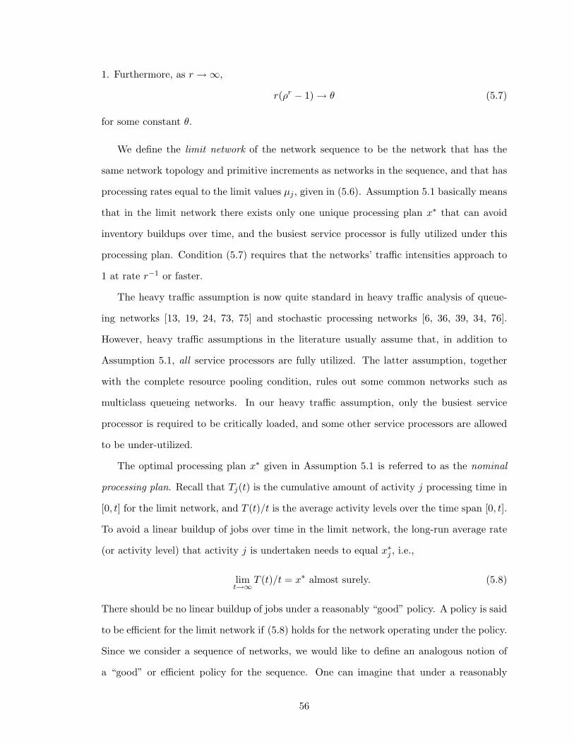
1. Furthermore, as r →∞,
r(ρr − 1) → θ (5.7)
for some constant θ.
We define the limit network of the network sequence to be the network that has the
same network topology and primitive increments as networks in the sequence, and that has
processing rates equal to the limit values µj , given in (5.6). Assumption 5.1 basically means
that in the limit network there exists only one unique processing plan x∗ that can avoid
inventory buildups over time, and the busiest service processor is fully utilized under this
processing plan. Condition (5.7) requires that the networks’ traffic intensities approach to
1 at rate r−1 or faster.
The heavy traffic assumption is now quite standard in heavy traffic analysis of queue-
ing networks [13, 19, 24, 73, 75] and stochastic processing networks [6, 36, 39, 34, 76].
However, heavy traffic assumptions in the literature usually assume that, in addition to
Assumption 5.1, all service processors are fully utilized. The latter assumption, together
with the complete resource pooling condition, rules out some common networks such as
multiclass queueing networks. In our heavy traffic assumption, only the busiest service
processor is required to be critically loaded, and some other service processors are allowed
to be under-utilized.
The optimal processing plan x∗ given in Assumption 5.1 is referred to as the nominal
processing plan. Recall that Tj(t) is the cumulative amount of activity j processing time in
[0, t] for the limit network, and T (t)/t is the average activity levels over the time span [0, t].
To avoid a linear buildup of jobs over time in the limit network, the long-run average rate
(or activity level) that activity j is undertaken needs to equal x∗j , i.e.,
limt→∞
T (t)/t = x∗ almost surely. (5.8)
There should be no linear buildup of jobs under a reasonably “good” policy. A policy is said
to be efficient for the limit network if (5.8) holds for the network operating under the policy.
Since we consider a sequence of networks, we would like to define an analogous notion of
a “good” or efficient policy for the sequence. One can imagine that under a reasonably
56

“good” policy, when r is large, the average activity levels over long time spans must be very
close to the nominal processing plan x∗. To be specific, we define the notion of asymptotic
efficiency as follows. Let T r be the cumulative activity level process for the r-th network.
Definition 5.2 (Asymptotic efficiency). Consider a sequence of stochastic processing
networks indexed by r = 1, 2, . . ., where Assumption 5.1 holds. A policy π is said to be
asymptotically efficient if and only if under policy π, with probability 1, for each t ≥ 0,
T r(r2t)/r2 → x∗t as r →∞. (5.9)
Equation (5.9) basically says that, under an asymptotically efficient policy, the average
activity levels over a time span of order r2 are very close to the nominal processing plan,
so that no linear buildup of jobs will occur over the time span of this order.
Remark. Asymptotic efficiency is closely related to the throughput optimality as de-
fined in Chapter 4. Fluid models have been used to prove the throughput optimality of a
stochastic processing network operating under a policy. Similarly, the fluid model corre-
sponding to the limit network can be used to prove the asymptotic efficiency of a policy for
the sequence of networks that satisfies Assumption 5.1. In particular, one can prove that a
policy π is asymptotically efficient if the fluid model of the limit network operating under
π is weakly stable.
The following theorem says that a maximum pressure policy is asymptotically efficient
for a sequence of networks if the limit network satisfies the EAA assumption, Assump-
tion 4.1.
Theorem 5.1. Consider a sequence of stochastic processing networks with Assumption 5.1
assumed. If the limit network satisfies the EAA assumption, Assumption 4.1, then a maxi-
mum pressure policy is asymptotically efficient.
The proof of Theorem 5.1 is almost identical to the proof of Theorem 4.2 in Chapter 4,
and will be outlined in Appendix B.
Asymptotic efficiency helps to identify reasonably “good” policies, but it is not very
discriminating. We would like to demonstrate certain sense of optimality for maximum
57

pressure policies in terms of secondary performance measures. For this, we will introduce
a notion of asymptotic optimality. The performance measure for our asymptotic optimality
is in terms of the workload process introduced in Section 5.1.
We focus on networks with a single bottleneck pool and assume the following:
Assumption 5.2 (Complete resource pooling). All networks in the sequence and the
limit network satisfy the complete resource pooling condition defined in Section 5.1. Namely,
the dual static planning problem (5.1)–(5.5) of the r-th network has a nonnegative, unique
optimal solution (yr, zr), and the dual static planning problem of the limit network also has
a nonnegative, unique optimal solution (y∗, z∗).
Under Assumption 5.2, we can define the one-dimensional workload process of the r-th
network as
W r(t) = yr · Zr(t).
Remark. In Assumption 5.2, we assume all networks in the sequence satisfy the com-
plete resource pooling condition so that the workload processes W r can be uniquely defined
as in Section 5.1 by the first order network data (Rr, Ar). This assumption can be removed
if one defines the workload process of a network with multiple bottleneck pools to be the
workload process of an arbitrarily chosen but prespecified bottleneck pool (with yr be any
given optimal solution to the dual problem). On the other hand, the complete resource
pooling condition for the limit network is crucial for our result to hold.
Definition 5.3 (Asymptotic optimality). Consider a sequence of stochastic processing
networks indexed by r. An asymptotically efficient policy π∗ is said to be asymptotically
optimal if and only if for any t > 0, w > 0, and any asymptotically efficient policy π,
lim supr→∞
P(W r
π∗(r2t)/r > w)≤ lim inf
r→∞P(W r
π(r2t)/r > w), (5.10)
where W rπ∗(·) and W r
π(·) are the workload processes under policies π∗ and π, respectively.
Define the diffusion-scaled workload process of the r-th network W r = {W r(t), t ≥ 0}
via W r(t) = W r(r2t)/r. Equation (5.10) says that, at every time t, asymptotically, the
58

diffusion-scaled workload under policy π∗ is dominated by that of any other asymptotically
efficient policy π in the sense of stochastic ordering.
To state our main theorem, we make a moment assumption on the unitized service times
uj(`) and an assumption on the initial queue length processes.
Assumption 5.3. There exists an εu > 0 such that, for all j,
E[(uj(1))2+εu
]<∞.
Assumption 5.3 requires that the unitized service times have finite 2 + εu moments. It
was introduced by Ata and Kumar [6], and it is stronger than some standard regularity
assumptions such as in Bramson [12]. Assumption 5.3 will be used in Section 5.5 to prove
a state space collapse result for stochastic processing networks operating under maximum
pressure policies.
We also assume that the queue length processes of the stochastic processing networks
satisfy the following initial condition. Define the diffusion-scaled queue length process Zr
via Zr(t) = Zr(r2t)/r, and let
ζr =yr
yr · yr. (5.11)
Assumption 5.4 (Initial condition). There exists a random variable wo such that
W r(0) → wo in distribution, (5.12)
and
|Zr(0)− ζrW r(0)| → 0 in probability. (5.13)
Assumption 5.4 holds if the initial queue lengths of the networks are stochastically
bounded, namely,
limτ→∞
lim supr→∞
P(|Zr(0)| > τ) = 0.
In this case, Zr(0) → 0 in probability.
Theorem 5.2 (Asymptotic Optimality). Consider a sequence of stochastic processing
networks. Assume Assumptions 5.1-5.4 and that the limit network satisfies the EAA as-
sumption. Maximum pressure policies are asymptotically optimal.
59

Hereafter, we shall assume Assumptions 5.1–5.4 and that the limit network satisfies the
EAA assumption.
Minimizing workload is important even if the ultimate objective is to optimize some
other secondary performance measures [6, 8, 36, 64]. For example, in Ata and Kumar [6], the
authors demonstrated that their discrete review policies are asymptotically optimal in linear
holding costs. They first proved the asymptotic optimality on the workload process. Then
the desired asymptotic optimality was achieved because the workload is “appropriately”
distributed under the discrete review policies.
Remark. Our asymptotic optimality is defined among the asymptotically efficient
policies. One natural question is whether the maximum pressure policies perform better, in
terms of equation (5.10), than the policies that are not asymptotically efficient. When the
optimal solution (y∗, z∗) to the dual problem (5.1)–(5.5) satisfies y∗ > 0, it can be proved
that the workload process under a maximum pressure policy is stochastically dominated by
the workload process under any policy. In fact, one can show that, under a policy that is not
asymptotically efficient, at least one component of the diffusion-scaled queue length process
Zr(t) will increase without bound almost surely for any t > 0 as r → ∞. This implies
that W r(t) increases without bound almost surely under the inefficient policy. Although
we believe that this is still true when y∗i = 0 for some i, we cannot provide a proof at this
point.
5.3 Outline of the Proof of Asymptotic Optimality
This section outlines the proof of our main asymptotic optimality theorem, Theorem 5.2.
We first derive an asymptotic lower bound on the workload processes under asymptoti-
cally efficient policies. Then we state a heavy traffic limit theorem, which implies that this
asymptotic lower bound is achieved by the maximum pressure policies. At the end, we
outline a proof, for the heavy traffic limit theorem, based on Bramson-Williams’ frame-
work [12, 74, 75].
60

We first derive an asymptotic lower bound on the workload processes under asymptoti-
cally efficient policies. That is, we search for a process W ∗ such that under any asymptoti-
cally efficient policy
lim infr→∞
P(W r(t) > w
)≥ P
(W ∗(t) > w
), for all t and w.
We begin the analysis by defining a process Y r = {Y r(t), t ≥ 0} for the r-th network
via
Y r(t) = (1− ρr)t− yr ·RrT r(t). (5.14)
Since ρr is interpreted as the traffic intensity of the bottleneck pool, for each t ≥ 0, ρrt is
interpreted as the average total work contributed to the bottleneck pool from the exogenous
arrivals in [0, t], and (1−ρr)t represents the average total work that could have been depleted
by time t if the bottleneck pool is never idle. Because of the randomness of the processing
times, the idleness of the bottleneck pool will almost surely be incurred over time given the
system is not overloaded. Under a service policy and its corresponding activity level process
T r, the average total work that has been depleted by time t is given by
yr ·RrT r(t) =∑j∈JS
T rj (t)
∑i∈I
yriR
rij −
∑j∈JI
T rj (t)
∑i∈I
yri (−Rr
ij).
Note that, as in Section 5.1, for each service activity j ∈ JS ,∑
i∈I yriR
rij is the average
work accomplished by per unit of activity j, and that for each input activity j ∈ JI ,∑i∈I y
ri (−Rr
ij) is the average work generated by per unit of activity j. Therefore, Y r(t)
represents the deviation of the workload depletion in [0, t] from that under the “best” policy.
The following lemma says that this deviation does not decrease over time.
Lemma 5.1. For each r and each sample path, the process Y r defined in (5.14) is a non-
decreasing function with Y r(0) = 0.
We leave the proof to Appendix B.
Remark. Some special stochastic processing networks, such as multiclass queueing
networks and unitary networks, have no control on the input activities. Then, T rj (t) is fixed
for all j ∈ JI under different policies, and∑
j∈JIT r
j (t)∑
i∈I yri (−Rr
ij) = ρrt. For these
61

networks, one gets
Y r(t) = t−∑j∈JS
T rj (t)
∑i∈I
yriR
rij ,
and Y r(t) is interpreted as the cumulative idle time of the bottleneck pool by time t.
From the flow balance equation (2.5) for the r-th network, we can write the workload
process W r = yr · Zr as
W r(t) = W r(0) +∑i∈I
yri
∑j∈J
(∑i′∈Bj
Φji′i
(Sr
j
(T r
j (t)))−BjiS
rj
(T r
j (t))),
where Srj (t) = max{n :
∑n`=1 uj(`) ≤ µr
jt}.
Let Xr = W r − Y r. Then one can check that
Xr(t) = W r(0)+∑i∈I
yri
∑j∈J
(∑i′∈Bj
Φji′i
(Sr
j
(T r
j (t)))−BjiS
rj
(T r
j (t)))−(1−ρr)t+yr ·RrT r(t).
We define the following diffusion-scaled processes:
Srj (t) = r−1
[Sr
j (r2t)− µr
jr2t]
for each j ∈ J ,
Φji′i(t) = r−1
[Φj
i′i(br2tc)− P j
i′ir2t]
for each j ∈ J and each i ∈ Bj ,
Xr(t) = r−1Xr(r2t),
Y r(t) = r−1Y r(r2t).
Here btc denotes the greatest integer number less than or equal to the real number t.
Then the diffusion-scaled workload process W r can be written as a sum of two processes
W r(t) = Xr(t) + Y r(t), (5.15)
and
Xr(t) = W r(0) +∑i∈I
yri
∑j∈J
(∑i′∈Bj
Φj,ri′i
(¯Srj
( ¯T rj (t)
))
+(∑
i′∈Bj
P ji′i −Bji
)Sr
j
( ¯T rj (t)
))− r(1− ρr)t, (5.16)
where
¯T rj (t) = r−2T r
j (r2t) and ¯Srj (t) = r−2Sr
j (r2t).
62

The process Xr depends on the policy only through the fluid-scaled process ¯T r. In fact, from
Lemma 4.1 of Dai [21] and (5.9), it follows that, under any asymptotically efficient policy,
¯T r ⇒ x∗(·), where x∗(t) = x∗t and x∗ is the optimal solution to the static planning prob-
lem (4.2)-(4.6) of the limit network. As a consequence, Xr converge to a one-dimensional
Brownian motion independent of policies.
Lemma 5.2. Consider a sequence of stochastic processing networks operating under an
asymptotically efficient policy. Then Xr ⇒ X∗, where X∗ is a one-dimensional Brownian
motion that starts from wo given in (5.12), has drift parameter θ given in (5.7), and has
variance parameter
σ2 = (y∗)′
∑j∈J
x∗jµj
∑i∈Bj
Υj,i
y∗ +∑i∈I
∑j∈J
(y∗i )2R2
ijx∗jµjσ
2j (5.17)
with Υj,i, j ∈ J , i ∈ Bj, defined by
Υj,ii1,i2
=
P ji,i1
(1− P ji,i2
), if i1 = i2,
−P ji,i1P j
i,i2, if i1 6= i2.
Proof. First, Lemma 4.1 of Dai [21] and (5.9) implies that ¯T r(·) ⇒ x∗(·) under any asymp-
totically efficient policy. Then, the result in the lemma follows from (5.16), the functional
central limit theorem for renewal processes (cf. Iglehart and Whitt [41]), the random time
change theorem (cf. Billingsley [11] (17.9)), and the continuous mapping theorem (cf.
Billingsley [11] Theorem 5.1). Deriving the expression for σ2 is straightforward but tedious,
which is outlined in [33] for multiclass queueing networks, so we will not repeat here.
We define the one-dimensional reflection mapping ψ : D[0,∞) → D[0,∞) such that for
each f ∈ D[0,∞) with f(0) ≥ 0,
ψ(f)(t) = f(t)−min(0, inf
0≤s≤tf(s)
).
Applying diffusion scaling to Lemma 5.1, we know that Y r(·) is a nonnegative, non-
decreasing function, so, from (5.15) and the well-known minimality of the solution of the
one-dimensional Skorohod problem (cf. Williams [9] Proposition B.1),
W r(t) ≥ ψ(Xr)(t) for every t and every sample path;
63

namely, ψ(Xr)(t) is a pathwise lower bound on W r. It then follows that
lim infr→∞
P(W r(t) > w) ≥ lim supr→∞
P(ψ(Xr)(t) > w), for all t and w.
Because Xr ⇒ X∗, by the continuous mapping theorem, we have
ψ(Xr) ⇒W ∗,
where W ∗ = ψ(X∗) is a one-dimensional reflecting Brownian motion associated with X∗.
Because W ∗(t) has continuous distribution for each t, we have
limr→∞
P(ψ(Xr)(t) > w) = P(W ∗(t) > w).
Therefore,
lim infr→∞
P(W r(t) > w) ≥ P(W ∗(t) > w) for each t and w.
So far, we have shown that W ∗ is an asymptotic lower bound on the workload processes
under asymptotically efficient policies. The following heavy traffic limit theorem ensures
that the workload processes under maximum pressure policies converge to W ∗. This com-
pletes the proof of Theorem 5.2.
Theorem 5.3 (Convergence). Consider a sequence of stochastic processing networks
operating under a maximum pressure policy. Assume Assumptions 5.1-5.4 in Section 5.2
and that the limit network satisfies the EAA assumption. Then
(W r, Zr) ⇒ (W ∗, Z∗) as r →∞,
where Z∗ = ζW ∗ with ζ defined as
ζ =y∗
y∗ · y∗. (5.18)
Theorem 5.3 also states a form of state space collapse for the network processes in the
diffusion limit: The I-dimensional queue length process is a constant vector multiple of the
one-dimensional workload process.
We will apply Bramson-Williams’ framework [12, 74, 75] to prove Theorem 5.3. The
framework consists of three steps that we will follow in the next three sections: First, in
Section 5.4, we will show that any fluid model solution for the stochastic processing networks
64

under maximum pressure policies exhibit some type of state space collapse, which is stated
in Theorem 5.4 in that section. Then, in Section 5.5, we will follow Bramson’s approach [12]
to translate the state space collapse of the fluid model into a state space collapse result under
diffusion scaling which is to be presented in Theorem 5.5. Finally, in Section 5.6, we will
convert the state space collapse result to the heavy traffic limit theorem, Theorem 5.3, by
applying a perturbed Skorohod mapping theorem from Williams [74].
5.4 State Space Collapse for the Fluid Model
In this section, we show that any fluid model solution under the maximum pressure policy
exhibits a form of state space collapse.
Theorem 5.4. Consider a sequence of stochastic processing networks that satisfy Assump-
tions 5.1 and 5.2. There exists some finite τ0 > 0, which depends on just I, R, and A, such
that, for any fluid model solution (Z, T ) under the maximum pressure policy, which satisfies
equations (4.7)–(4.11) and (4.13), if |Z(0)| ≤ 1, then
|Z(t)− ζW (t)| = 0, for all t ≥ τ0, (5.19)
where W = y∗ · Z is the workload process of the fluid model and ζ is given by (5.18).
Furthermore, if
|Z(τ1)− ζW (τ1)| = 0, for some τ1 ≥ 0,
then
|Z(t)− ζW (t)| = 0, for all t ≥ τ1. (5.20)
Theorem 5.4 says that the fluid model under maximum pressure policy exhibits a form
of state space collapse: after some finite time τ0, the I-dimensional buffer level process
Z equals a constant vector multiple of the one-dimensional workload process W ; if this
happens at time τ1, it happens all the time after τ1. In particular, if Z(0) = ζW (0), then
Z(t) = ζW (t) for all t.
The rest of this section is to prove Theorem 5.4. We first define
Z∗(t) = ζW (t),
65

and we shall prove Z(t)− Z∗(t) = 0 for t large enough. Because Z∗(t) is the projection of
Z(t) on y∗, Z(t)− Z∗(t) is orthogonal to y∗. Therefore, we have the following lemma.
Lemma 5.3. For any t ≥ 0, (Z(t)− Z∗(t)
)· y∗ = 0,
and for each regular time t,
(Z(t)− Z∗(t)
)· ˙Z∗(t) = 0.
Proof.
Z∗(t) · y∗ = W (t)ζ · y∗ = W (t) = Z(t) · y∗.
Because ˙Z∗(t) = ζ ˙W (t),
(Z(t)− Z∗(t)
)· ˙Z∗(t) = ˙W (t)
(Z(t)− Z∗(t)
)· ζ = 0.
The following lemma will be used repeatedly in subsequel. It follows directly from
Lemma A.1 to be presented in Appendix A.
Lemma 5.4. Suppose (y, z) is a unique optimal solution to the dual problem (5.1)–(5.5)
with objective value ρ. Then y is the unique I-dimensional vector that satisfies
maxa∈A
∑i∈I,j∈JS
yiRijaj = 1, (5.21)
and
maxa∈A
y ·Ra = 1− ρ. (5.22)
Define V = {Ra : a ∈ A}. Recall that A is the set of all possible allocations and the
vector Ra is the average rate at which material consumed from all buffers under allocation
a, so V is the set of all possible flow rate out of buffers in the limit network. It is obvious
that V is a polytope containing the origin because Rx∗ = 0, where, as before, x∗ is the
optimal solution to the static planning problem of the limit network. Furthermore, from
Lemma 5.4 and the fact that ρ∗ = 1 for the limit network, we have
maxv∈V
y∗ · v = 0.
66

It says that the outer normal of V at the origin is y∗. Then, V is in a half space separated
by the (I − 1) dimensional hyperplane V o = {v ∈ RI : y∗ · v = 0}. The hyperplane V o
is orthogonal to y∗ and passes the origin, so V ∩ V o is not empty. Furthermore, in the
hyperplane V o, there exists some (I − 1) dimensional neighborhood of the origin that is a
subset of V . This is stated in the following proposition.
Proposition 5.1. There exists some δ > 0 such that {v ∈ V o : ‖v‖ ≤ δ} ⊂ V .
Proof. First, if the statement is not true, then we can find a v0 ∈ V o such that κv0 6∈ V for
all 0 < κ ≤ 1 because of the convexity of V . Denote V0 = {κv0, 0 < κ < 1}. Because any v
in V0 is not in V , V0 ∩ V = ∅. It is easy to see that V0 is open and convex. Therefore there
exists a hyperplane separating V and V0 (cf. Rudin [60] Theorem 3.4 ). In other words,
there exists a vector y and a constant b such that y · v ≤ b for all v ∈ V and y · v > b for all
v ∈ V0. We notice that b must be zero. To see this, first we have b ≥ 0 because the origin
is in V . Moreover, for any ε > 0, we can choose κ arbitrarily small such that κy · v0 < ε.
Because κv0 ∈ V0, we have b < κy · v0 < ε. This implies b = 0, therefore the origin is in the
separating hyperplane and maxa∈A y ·Ra = 0. Obviously, y 6= y∗ because y∗ · v = 0 > y · v
for v ∈ V0. We consider two cases:
Case 1: maxa∈A∑
i∈I,j∈JSyiRijaj > 0. For this case, without loss of generality, we select
y such that maxa∈A∑
i∈I,j∈JSyiRijaj = 1. Then y satisfies both (5.21) and (5.22)
with ρ = 1. On the other hand, from Lemma 5.4, y∗ is the unique vector that satisfies
both (5.21) and (5.22). This is a contradiction.
Case 2: maxa∈A∑
i∈I,j∈JSyiRijaj = 0. For this case, one can verify that y∗ + y satisfies
both (5.21) and (5.22) with ρ = 1. This is also a contradiction.
The set V ∗ = V ∩ V o is the set of all possible flow rates that maximize y∗ · v; namely,
V ∗ = argmaxv∈V y∗ · v.
Proof of Theorem 5.4. We consider the Lyapunov function f(t) = ‖Z(t) − Z∗(t)‖2. Let
v(t) = R ˙T (t) denote the net flow rate out of the system at time t (total departure rate
67

minus total arrival rate). Then ˙Z(t) = −v(t), and we have
f(t) = 2(Z(t)− Z∗(t)
)·(
˙Z(t)− ˙Z∗(t))
= 2(Z(t)− Z∗(t)
)· (−v(t)) (5.23)
The second equality in (5.23) follows from Lemma 5.3.
Because ˙T (t) ∈ A, we have v(t) ∈ V . This implies that y∗ · v(t) ≤ 0 and hence
Z∗(t) · v(t) ≤ 0. Furthermore, under maximum pressure policies, it follows from the fluid
model equation that v(t) satisfies
v(t) · Z(t) = maxv∈V
Z(t) · v.
Therefore the last term in (5.23) is bounded from above as follows.
2(Z(t)− Z∗(t)) · (−v(t)) ≤ −2Z(t) · v(t) = −2 maxv∈V
(Z(t) · v
)(5.24)
Since V ∗ ⊂ V , we have
maxv∈V
Z(t) · v ≥ maxv∈V ∗
(Z(t) · v
)= max
v∈V ∗
((Z(t)− Z∗(t)
)· v). (5.25)
The second equality in (5.25) holds because y∗ · v = 0 for all v ∈ V ∗ and Z∗(t) = ζW (t).
If f(t) > 0, let
v∗ =δ(Z(t)− Z∗(t))‖Z(t)− Z∗(t)‖
.
Then ‖v∗‖ = δ and y · v∗ = 0. It follows from Proposition 5.1 that v∗ ∈ V ∗. Therefore
maxv∈V ∗
(Z(t)− Z∗(t)) · v ≥ (Z(t)− Z∗(t)) · v∗ = δ‖Z(t)− Z∗(t)‖. (5.26)
Combining (5.23)–(5.26), we have
f(t) ≤ −2δ‖Z(t)− Z∗(t)‖ = −2δ√f(t). (5.27)
Therefore f(t) = 0 for t ≥√f(0)/δ. Set τ0 =
√I/δ. Then f(t) = 0 for t ≥ τ0, because
f(0) = (Z(0)− Z∗(0)) · (Z(0)− Z∗(0)) = (Z(0)− Z∗(0)) · Z(0) ≤ ‖Z(0)‖2 ≤ I.
Here τ0 depends only on R, A, and I, because the set V is completely determined by R and
A and so is δ.
Equation (5.27) also implies that for any τ1, if f(τ1) = 0 then f(t) = 0 for all t ≥ τ1.
68

5.5 State Space Collapse
In this section, we translate the state space collapse result of the fluid model into a state
space collapse result under diffusion scaling.
Theorem 5.5 (State Space Collapse). Consider a sequence of stochastic processing
networks operating under a maximum pressure policy. Assume Assumptions 5.1–5.4 and
that the limit network satisfies the EAA assumption. Then, for each T ≥ 0,
‖Zr(·)− ζrW r(·)‖T → 0 in probability.
Recall that ζr was given in (5.11) and ‖·‖T is the uniform norm over [0, T ]. (The readers
should not confuse the symbols T and T (·) with one another. We will always include “(·)”
when dealing with the cumulative activity level process T (·).)
Theorem 5.5 states a form of state space collapse for the diffusion-scaled network process:
for large r, the I-dimensional diffusion-scaled queue length process is essentially a constant
vector multiple of the one-dimensional workload process .
The rest of this section applies Bramson’s approach [12] to prove Theorem 5.5. In
Bramson’s approach, the following fluid scaling plays an important role in connecting The-
orems 5.4 and 5.5: For each r = 1, 2, . . ., and m = 0, 1, . . .,
Sr,mj (t) =
1ξr,m
(Sr
j (rm+ ξr,mt)− Srj (rm)
), for each j ∈ J ,
Φj,r,mi (t) =
1ξr,m
(Φj
i
(Sr
j (rm) + bξr,mtc)− Φj
i
(Sr
j (rm))), for each j ∈ J , i ∈ Bj ,
T r,mj (t) =
1ξr,m
(T r
j (rm+ ξr,mt)− T rj (rm)
), for each j ∈ J ,
Zr,mi (t) =
1ξr,m
Zri (rm+ ξr,mt), for each i ∈ I,
where ξr,m = |Zr(rm)| ∨ r.
Here scaling the processes by ξr,m ensures |Zr,m(0)| ≤ 1, which is needed for compactness
reasons. And using index (r,m) allows the time scale to expand; we will examine the
processes over [0, L] for m = 0, 1, . . . , drT e − 1, where L > 1 and T > 0 are fixed, so the
diffusion-scaled time [0, T ] is covered by drT e fluid scaled time pieces, each with length
L ≥ 1. Here dte denotes the smallest integer greater than or equal to t.
69

We outline the proof of Theorem 5.5 as follows. First, in Proposition 5.2, we give
a probability estimate on the upper bound of the fluctuation of the stochastic network
processes Xr,m(·) = (T r,m(·), Zr,m(·)). The estimates on the service processes Sr,mj (·) and
the routing processes Φj,r,mi (·) are also given. From Proposition 5.2, a so-called “good”
set Gr of sample paths can be defined, where the processes Xr,m perform nicely for r large
enough. On this “good” set, for large enough r, the processes Xr,m can be uniformly
approximated by so-called Lipschitz cluster points. These cluster points will be shown to be
fluid model solutions under the maximum pressure policy. Then because of Theorem 5.4,
the state space collapse of the fluid model under the maximum pressure policy, the network
processes Xr,m asymptotically have the state space collapse, which then will be translated
into the state space collapse for diffusion-scaled processes Xr as r approaches ∞.
Notice that in Theorem 5.5 the state space collapse of the fluid model does not happen
instantaneously after time 0 if the initial state does not exhibit a state space collapse. The
fluid-scaled processes Xr,m start from time rm in the original network processes, so, for
m ≥ 1, Xr,m do not automatically have the state space collapse at the initial point, and
only the interval [τ0, L] can be used for our purpose. However, for m = 0, the state space
happens at time 0 because of the initial condition (5.13), so the whole interval [0, L] can be
used. For this reason, we separate the proof into two parts according to the two intervals
in the diffusion-scaled time: [0, Lξr,0/r2] and [τ0ξr,0/r2, T ].
Propositions 5.3–5.6 develop a state space collapse on the interval [τ0ξr,0/r2, T ]. Propo-
sition 5.3 shows that, on Gr, the scaled process Xr,m(·) are uniformly close to Lipschitz
cluster points for large r. Proposition 5.4 shows that the above cluster points are solutions
to the fluid model equations. Propositions 5.3 and 5.4 together with Theorem 5.4, the state
space collapse for the fluid model under the maximum pressure policy, imply the state space
collapse of the fluid scaled processes Xr,m(·) on Gr and the interval [τ0, L], which is the result
of Proposition 5.5. The result is translated into diffusion scaling, and Proposition 5.6 gives
a version of state space collapse for the diffusion process Xr(t) on the interval [τ0ξr,0/r2, T ].
The state space collapse on the interval [0, Lξr,0/r2] are shown through Propositions 5.7–
5.9. The basic idea is the same as described in the preceding paragraph except that now
70

we only consider the scaled processes with m = 0. The corresponding network processes
start from time 0, and by assuming the state space collapse happens at time 0, we have
stronger result for these type of processes: the state space collapse holds during the whole
time interval [0, L] instead of just on [τ0, L]. In fact, the scaled processes Xr,0(·) are proven
to be uniformly close to some cluster points for which the state space collapse starts at time
0. This is stated in Propositions 5.7 and 5.8. In Proposition 5.9, we summarize the state
space collapse for fluid scaled process on [0, L] and translate it into the diffusion scale on
[0, Lξr,0/r2].
The results to be obtained in Propositions 5.6 and 5.9 are actually multiplicative state
space collapse, as called in Bramson [12]. To obtain the state space collapse result that we
stated in Theorem 5.5, we will prove ξr,m/r are stochastically bounded at the end of this
section.
5.5.1 Probability estimates
In this section, we give probability estimates on the service processes Sr,mj (·), the rout-
ing processes Φj,r,mi (·), and the upper bound of the fluctuation of the stochastic network
processes Xr,m(·).
Proposition 5.2. Consider a sequence of stochastic processing networks where the moment
assumption, Assumption 5.3 is assumed. Fix ε > 0, L and T . Then, for large enough r,
P( maxm<rT
‖Sr,mj (T r,m
j (t))− µrjT
r,mj (t)‖L > ε) ≤ ε, for each j ∈ J , (5.28)
P( maxm<rT
‖Φj,r,mi (Sr,m
j (T r,mj (t)))− P j
i µrj(T
r,mj (t))‖L > ε) ≤ ε, for each j ∈ J and i ∈ Bj ,
(5.29)
P( sup0≤t1≤t2≤L
|Xr,m(t2)− Xr,m(t1)| > N |t2 − t1|+ ε for some m < rT ) ≤ ε, (5.30)
where N is some constant that depends on just the bounds of Rr.
To prove Proposition 5.2, we first need the following lemma.
Lemma 5.5. Assume that the moment assumption, Assumption 5.3, holds. Then for given
T , and each j ∈ J
ur,T,maxj /r → 0 as r →∞ with probability 1, (5.31)
71

where ur,T,maxj = max{uj(`) : 1 ≤ ` ≤ Sr
j (r2T ) + 1}. Furthermore, for any given ε > 0,
P(‖Φji (`)− P j
i `‖n ≥ εn) ≤ ε/n, for each j ∈ J and i ∈ Bj , and large enough n, (5.32)
and for large enough t,
P(‖Srj (τ)− µr
jτ‖t ≥ εt) ≤ ε/t, for all j ∈ J , and all r. (5.33)
We delay the proof of Lemma 5.5 to Appendix B, and now we are ready to prove
Proposition 5.2.
Proof of Proposition 5.2. The proof here essentially follows the same reasoning as in Propo-
sitions 5.1 and 5.2 of Bramson [12]. We first investigate the processes with index m, and
then multiply the error bounds by the number of processes in each case, drT e. We first
start with (5.28). From (5.31), we have, for large enough r,
P(ur,T,maxj /r ≥ ε) ≤ ε/2. (5.34)
Denote Mr to be the complement of the events in (5.34). Then, for large enough r,
P(Mr) ≥ 1− ε/2. (5.35)
Let τ be the time that the first activity j service completion occurs after time rm. Then
from (5.33), for large enough r, we have
P(‖Sr
j
(rm+ ξr,mT
r,mj (t)
)− Sr
j (τ)− µrj
(rm+ ξr,mT
r,mj (t)− τ
)‖L ≥ εLξr,m
)≤ ε/Lr;
we use the fact that T r,mj (t) ≤ t, ξr,m ≥ r, and Sr
j (rm+ ξr,mTr,mj (t))−Sr
j (τ) is independent
of ξr,m. Because Srj (τ) = Sr
j (rm) + 1 and τ − rm ≤ ur,T,maxj /µr
j , we have
P(‖Sr
j
(rm+ ξr,mT
r,mj (t)
)− Sr
j (rm)− µrjξr,mT
r,mj (t))‖L ≥ |1− ur,T,max
j |+ εLξr,m
)≤ ε/Lr.
It follows that
P(‖Sr,mj (T r,m
j (t))− µrjT
r,mj (t)‖L ≥ 2εL |Mr) ≤ ε/Lr, for large enough r. (5.36)
Therefore, by multiplying the lower bound by drT e,
P( maxm≤rT
‖Sr,mj (T r,m
j (t))− µrjT
r,mj (t)‖L ≥ 2εL |Mr) ≤ εT.
72

Then enlarging ε by a factor of 2(L ∨ T ), we have
P( maxm≤rT
‖Sr,mj (T r,m
j (t))− µrjT
r,mj (t)‖L ≥ ε |Mr) ≤ ε/2.
This, together with (5.35) implies (5.28).
Let µmax be an upper bound on |µr|. Then from (5.36), for large enough r,
P(Sr,m
j
(T r,m
j (L))≥ (µmax + 2)L | Mr
)≤ ε/Lr.
By (5.32) with n = (µmax + 2)Lξr,m, we have for each i ∈ Bj ,
P(‖Φj,r,m
i
(Sr,m
j
(T r,m
j (t)))− P j
i Sr,mj
(T r,m
j (t))‖L > ε(µmax + 2)L | Mr
)≤ ε/(µmax + 2)Lξr,m + ε/Lr.
Let Pmax = maxj∈J ,i∈Bj |Pji |, then from (5.36), we have
P(‖P ji S
r,mj (T r,m
j (t))− P ji µ
rjT
r,mj (t)‖L ≥ 2PmaxεL |Mr) ≤ ε/Lr.
It follows that
P(‖Φj,r,m
i
(Sr,m
j
(T r,m
j (t)))− P j
i µrj
(T r,m
j (t))‖L > ε(2Pmax + µmax + 2)L | Mr
)≤ 5ε/2Lr.
Enlarging ε by a factor of (2Pmax + µmax + 2)L ∨ 5T and multiplying the error bound by
drT e, we have
P(
maxm≤rT
‖Φj,r,mi
(Sr,m
j
(T r,m
j (t)))−P j
i µrj
(T r,m
j (t))‖L > ε | Mr
)≤ ε/2.
Then (5.29) follows.
Now we are going to show (5.30). First, it is easy to see that, for each j ∈ J and each
r,
T rj (t)− T r
j (s) ≤ t− s for 0 ≤ s ≤ t
along any sample path. Therefore, the bounds in (5.30) on components Tj is easy to obtain
with N = 1. For components Zi, i ∈ I, scaling (2.5) and applying (5.28) and (5.29) gives
P(
sup0≤t1≤t2≤L
|Zr,mi (t2)− Zr,m
i (t1)|
> Rrij |T
r,mj (t2)− T r,m
j (t1)|+ 2J(I + 2)ε for some m ≤ rT
)≤ 2J(I + 2)ε.
73

Then (5.30) is obtained by enlarging ε in the above inequality by a factor of 2J(I + 1) and
setting N = 1 ∨ supr|Rr|.
Now for each large enough r, we let ε(r) be the smallest ε such that (5.28)-(5.30) are
satisfied. By Proposition 5.2, it is easy to see that
limr→∞
ε(r) = 0.
We consider the complements of the “bad” events given in each of (5.28)-(5.30) with ε
replaced by ε(r), and denote the intersection of these “good” events by Gr. Obviously
limr→∞
P(Gr) = 1.
5.5.2 State space collapse on [ξr,0τ0/r2, T ]
We divide the diffusion-scaled time interval [0, T ] into two overlapping intervals: [0, ξr,0L/r2]
and [ξr,0τ0/r2, T ]. In this section, we show a state space collapse result on the time interval
[ξr,0τ0/r2, T ]. The state space collapse on [0, ξr,0L/r2] will be presented in the next section.
In order to connect the fluid-scaled processes with the fluid model, we first introduce
the notion of cluster point. Let F = Dd[0, L] with d = I + J, so F is the space of right
continuous functions with left limits from [0, L] to RI+J. Let F = {Fr} be a sequence of
subsets in F . A cluster point f of F is defined to be a point f ∈ F such that for all ε > 0
and r0 > 0, there exists r ≥ r0 and g ∈ Fr, with ‖f − g‖L < ε. Now, let Fr, r = 1, 2, . . ., be
certain subsets of F , where all elements f satisfy both
|f(0)| ≤ 1 (5.37)
and
|f(t2)− f(t1)| ≤ N |t2 − t1|+ ε(r) for all t1, t2 ∈ [0, L], (5.38)
with constant N chosen as in Proposition 5.2 and ε(r) → 0 as r →∞. The sequence {Fr}
is said to be asymptotically Lipschitz. Let F ′ denote those f ∈ F satisfying both (5.37) and
|f(t2)− f(t1)| ≤ N |t2 − t1| for all t1, t2 ∈ [0, L] (5.39)
The following lemma is due to Bramson [12]. We reproduce it here for completeness.
74

Lemma 5.6 (Bramson [12] Proposition 4.1). For each ε > 0, there exists an r0, so
that for each r ≥ r0 and g ∈ Fr, one has ‖f − g‖L < ε for some cluster point f of F with
f ∈ F ′.
Lemma 5.6 says that, for large r, each element of the function sets in an asymptotically
Lipschitz sequence can be uniformly approximated by a cluster point that is Lipschitz
continuous.
We set
F rg = {Xr,m(·, ω), m < rT, ω ∈ Gr} for each r,
and
Fg = {F rg }.
From the choice of the fluid scale ξr,m and the definition of T r,m(·), it follows that
|Xr,m(0)| ≤ 1,
so (5.30) in Proposition 5.2 implies that the sequence of sets of scaled stochastic processing
network processes Xr,m(·) is asymptotically Lipschitz. Then Lemma 5.6 immediately implies
the following Proposition which says that Xr,m(·) are uniformly close to Lipschitz cluster
points Xr,m(·) for large r.
Proposition 5.3. Fix ε > 0, L and T , and choose r large enough. Then, for ω ∈ Gr and
any m < rT ,
‖Xr,m(·, ω)− X(·)‖L ≤ ε
for some cluster point X(·) of Fg with X(·) ∈ F ′.
The next proposition says that if the stochastic processing networks operate under a
maximum pressure policy, then each cluster point of Fg is a fluid model solution under the
maximum pressure policy and satisfies fluid model equations (4.7)–(4.11) and (4.13).
Proposition 5.4. Consider a sequence of stochastic processing networks operating under
a maximum pressure policy. Assume Assumption 5.1 and that the limit network satisfies
the EAA assumption. Fix L and T . Then all cluster points of Fg are solutions to the fluid
model equations (4.7)–(4.11) and (4.13) on [0, L].
75

Proof. The idea is to approximate each cluster point of Fg with some Xr,m on Gr and show
that the equations (4.7)–(4.11) and (4.13) are asymptotically satisfied by Xr,m. We will
only demonstrate equations (4.7) and (4.13); the others are quite straightforward and can
be verified similarly. We first verify equation (4.7). For any ε > 0, we can choose large
enough r, and appropriate ω ∈ Gr and m < rT , such that
‖Sr,mj (T r,m
j (t))− µrjT
r,mj (t)‖L ≤ ε for each j ∈ J , (5.40)
‖Φj,r,mi
(Sr,m
j (T r,mj (t))
)− P j
i µrjT
r,mj (t)‖L ≤ ε, for each j ∈ J , i ∈ Bj , (5.41)
‖Z(·)− Zr,m(·)‖L ≤ ε, (5.42)
‖T (·)− T r,m(·)‖L ≤ ε, (5.43)
|Rr −R| ≤ ε. (5.44)
Scaling (2.5) and plugging in the bounds in (5.40) and (5.41), we have
|Zr,m(t)− Zr,m(0)−RrT r,m(t)| ≤ 2ε for each t ≤ L.
From (5.43) and (5.44), we have, for each t ≤ L,
|RrT r,m(t)−RT (t)| ≤ |Rr(T r,m(t)− T (t)|+ |(Rr −R)T (t)| ≤ NJε+ εNLJ.
Recall that N ≥ supr|Rr|. It then follows that, for each t ≤ L,
|Z(t)− Z(0)−RT (t)| ≤ |Z(t)− Zr,m(t)|+ |Zr,m(0)− Z(0)|+ |RrT r,m(t)−RT (t)|
+|Zr,m(t)− Zr,m(0)−RrT r,m(t)|
≤ (4 +NLJ +NJ)ε.
Then equation (4.7) is satisfied by X because ε can be arbitrarily small.
To show equation (4.13), first observe that for any allocation a ∈ A,
|p(Z(t), a)− pr(Zr,m, a)| = |Z(t) ·Ra− Zr,m(t) ·Rra|
≤ |Z(t) · (Ra−Rra)|+ |(Z(t)− Zr,m(t)) ·Rra|
≤ (NL+ 1)IJε+ εIJN.
Denote E∗ as the set of maximum extreme allocations under buffer size Z(t). Suppose
that a ∈ E \ E∗ and p(a, Z(t)) < maxa′∈E p(a′, Z(t)). Because the limit network satisfies the
76

EAA assumption, we can choose an a∗ ∈ E∗ such that Zi(t) > 0 for each constituent buffer
i of a∗. Denote I(a∗) the set of constituent buffers. Namely,
I(a∗) ={i :∑
j
a∗jBji > 0}.
Then Zi(t) > 0 for all i ∈ I(a∗). Since p(a, Z(t)) < p(a∗, Z(t)) and mini∈I(a∗) Zi(t) > 0, by
the continuity of X(·), there exist ε1 > 0 and δ > 0 such that for each τ ∈ [t− δ, t+ δ] and
i ∈ I(a∗),
p(a, Z(τ)) + ε1 ≤ p(a∗, Z(τ)) and Zi(τ) ≥ ε1.
For sufficiently large r, we can choose ε small enough such that (NL+N+1)IJε ≤ ε1/3.
Then, for all τ ∈ [t− δ, t+ δ],
pr(a, Zr,m(τ)) + ε1/3 ≤ pr(a∗, Zr,m(τ)),
Zr,mi (τ) ≥ ε1/2 for each i ∈ I(a∗).
Choosing r > 2J/ε1, for each τ ∈ [rm+ ξr,m(t− δ), rm+ ξr,m(t+ δ)], we have
pr(a, Zr(τ)) < pr(a∗, Zr(τ)), (5.45)
Zri (τ) ≥ J for each i ∈ I(a∗). (5.46)
Condition (5.46) implies that a∗ is a feasible allocation at any time τ ∈ [rm + ξr,m(t −
δ), rm + ξr,m(t + δ)], i.e., a∗ ∈ E(τ). Following (5.45) and the definition of a (preemptive-
resume) maximum pressure policy, the allocation a will not be employed during time interval
[rm+ ξr,m(t− δ), rm+ ξr,m(t+ δ)]. Therefore, only the allocations in E∗ will be employed
during this interval. For each a ∈ E , denote (T a)r(t) to be the cumulative amount of time
allocation a has been employed by time t. It is easy to see that, for each r and all t ≥ 0,
under the maximum pressure policy,
∑a∈E
(T a)r(t) = t, (5.47)
T r(t) =∑a∈E
a(T a)r(t). (5.48)
77

Then it follows that
Z(t) ·(R[T r(rm+ ξr,m(t+ δ)
)− T r
(rm+ ξr,m(t− δ)
)])=∑a∈E
(Z(t) ·Ra)[(T a)r
(rm+ ξr,m(t+ δ)
)− (T a)r
(rm+ ξr,m(t− δ)
)]=∑a∈E∗
(Z(t) ·Ra)[(T a)r
(rm+ ξr,m(t+ δ)
)− (T a)r
(rm+ ξr,m(t− δ)
)]= max
a∈A
∑a∈E∗
[(T a)r
(rm+ ξr,m(t+ δ)
)− (T a)r
(rm+ ξr,m(t− δ)
)]= max
a∈A
∑a∈E
[(T a)r
(rm+ ξr,m(t+ δ)
)− (T a)r
(rm+ ξr,m(t− δ)
)]= 2ξr,mδmax
a∈AZ(t) ·Ra.
(5.49)
The second and fourth equalities in (5.49) hold because only allocations in E∗ will be
employed during [rm+ξr,m(t−δ), rm+ξr,m(t+δ)]; the third holds because every allocation
a ∈ E∗ has the same network pressure equal to maxa∈A Z(t) ·Ra. From (5.49), we have
Z(t) ·R(T r,m(t+ δ)− T r,m(t− δ)
)/2δ = max
a∈AZ(t) ·Ra.
Because ε in (5.43) can be arbitrarily small, we have
Z(t) ·R(T (t+ δ)− T (t− δ)
)/2δ = max
a∈AZ(t) ·Ra,
and (4.13) is verified.
From Theorem 5.4, every fluid model solution under the maximum pressure policy sat-
isfies (5.19), so Proposition 5.4 implies that any cluster point X of Fg satisfies (5.19). That
is,
|Z(t)− ζW (t)| = 0 for t ≥ τ0,
where W (·) = y∗ · Z(t). Because the fluid-scaled stochastic processing network processes
can be uniformly approximated by cluster points, it leads to the following proposition.
Proposition 5.5. Fix L, T and ε > 0. For r large enough,
|Zr,m(t)− ζrW r,m(t)| ≤ ε for all 0 ≤ m ≤ rT, τ0 ≤ t ≤ L, ω ∈ Gr.
To prove Proposition 5.5, we first need yr → y∗ as r →∞.
78

Lemma 5.7. Assume Assumptions 5.1 and 5.2. Then, (yr, zr) → (y∗, z∗) as r →∞.
The proof of Lemma 5.7 will be provided in Appendix B.
Proof of Proposition 5.5. From Proposition 5.3, for large enough r and each 0 ≤ m ≤
rT, ω ∈ Gr, we can find a cluster point X such that
‖Z(·)− Zr,m(·)‖L ≤ ε.
From Proposition 5.4 and Theorem 5.4, we have
|Z(t)− ζW (t)| = 0 for t ≥ τ0.
Then, for each t ≥ τ0,
|Zr,m(t) − ζrW r,m(t)| ≤ |Zr,m(t) − Z(t)| + |ζW (t) − ζrW (t)| + |ζrW (t) − ζrW r,m(t)|.
(5.50)
Because yr → y∗ as r →∞, for large enough r,
|yr − y∗| < ε, and |ζr − ζ| < ε.
Let κ = (supr|yr|) ∨ (supr|ζr|). Then we have
|W (t)−W r,m(t)| ≤ |y · Z(t)− yr · Z(t)|+ |yr · Z(t)− yr · Z(t)|
≤ I(ε|Z(t)|+ κε
)≤ (L+ κ)Iε.
Note that Z(t) ≤ NL for all t ≤ L. One also gets W (t) ≤ κNL since |y∗| ≤ κ. From (5.50),
we have
|Zr,m(t)− ζrW r,m(t)| ≤ ε+ εIκNL+ κ(NL+ κ)Iε.
Rechoosing ε, the result follows.
We need to translate the results in Proposition 5.5 into the state space collapse results
under diffusion scaling. First we can express Zr,m(t) by Zr via
Zr,m(t) =r
ξr,mZr(
tξr,m + rm
r2) =
1ξr,m
Zr(tξr,m +m
r),
where ξr,m = ξr,m/r.
The interval [τ0, L] in Zr,m corresponds to the diffusion-scaled time interval [(m +
ξr,mτ0)/r, (m+ ξr,mL)/r], and Proposition 5.5 immediately leads to the following.
79

Proposition 5.6. Fix L > 0, T > 0 and ε > 0. For r large enough and each m < rT ,
|Zr(t)− ζrW r(t)| ≤ ξr,mε for all (m+ ξr,mτ0)/r ≤ t ≤ (m+ ξr,mL)/r, ω ∈ Gr. (5.51)
Proposition 5.6 gives estimates on each small interval for |Zr(t) − ζrW r(t)|. We shall
obtain the estimate on the whole time interval [0, T ], and then show ξr,m are stochastically
bounded. The following lemma ensures that for large enough L, L > 3NT , the small
intervals in Proposition 5.6 are overlapping, and therefore the estimate on [ξr,0τ0/r, T ] is
obtained.
Lemma 5.8. For fixed T and large enough r,
ξr,m+1 ≤ 3Nξr,m,
for ω ∈ Gr and m < rT .
Proof. By the definition of Gr,
|Zr,m(t2)− Zr,m(t1)| ≤ N |t2 − t1|+ 1.
for t1, t2 ∈ [0, L] and m < rT . Set t1 = 0 and t2 = 1/ξr,m, we have
|Zr ((m+ 1)/r) | − |Zr (m/r) | ≤ N + ξr,m.
Therefore,
ξr,m+1 ≤ |Zr ((m+ 1)/r) | ∨ 1 ≤(|Zr (m/r) |+N + ξr,m
)∨ 1 ≤ N + 2ξr,m ≤ 3Nξr,m.
5.5.3 State space collapse on [0, ξr,0L/r2]
Now we shall estimate |Zr(t) − ζrW r(t)| on the interval [0, ξr,0L/r]. This will be given by
the initial condition (5.13) and the result in the second part of Theorem 5.4.
Condition (5.13) implies that
|Zr,0(0)− ζrW r,0(0)| → 0 in probability.
80

Then, for each r > 0, we let
ε1(r) = min{ε : P(|Zr,0(0)− ζrW r,0(0)| > ε
)≤ ε}.
It is easy to see that
limr→∞
ε1(r) → 0.
Now let Lr be the subset of Gr such that for all events in Lr
|Zr,0(0)− ζrW r,0(0)| > ε1(r).
Obviously, limr→∞ P(Lr) = 1.
We define
Fo = {F ro }
with
F ro = {Xr,0(·, ω), ω ∈ Lr}.
Parallel to Proposition 5.3, we have the following proposition which states that Fo can
be asymptotically approximated by cluster points of Fo.
Proposition 5.7. Fix ε > 0, L and T , and choose r large enough. Then, for ω ∈ Lr,
‖Xr,0(·, ω)− X(·)‖L ≤ ε
for some cluster point X(·) of Fo with X(·) ∈ F ′.
Proof. Since both (5.37) and (5.39) are satisfied by Xr,m, the result follows from Lemma 5.6.
Proposition 5.8. Fix L. Then for any cluster point X(·) of Fo,
Z(t) = ζW (t) for t ≤ L.
Proof. Since any cluster point of Fo is automatically a cluster point of Fg, it satisfies all
the fluid model equations. Now we show that
|Z(0)− ζW (0)| = 0, (5.52)
81

which together with Theorem 5.4 implies the result.
For given δ > 0, one can choose r large enough so that
‖Xr,0(·)− X(·)‖L ≤ δ,
|Zr,0(0)− ζrW r,0(0)| ≤ δ,
and
|ζr − ζ| ≤ δ.
Let κ = supr |yr|. Then
|W r,0(0)| = |yr · Zr,0(0)| ≤ Iκ,
and
|W (0)−W r,0(0)| = |y∗ · Z(0)− yr · Zr,0(0)|
≤ |y∗ · (Z(0)− Zr,0(0)) + (y∗ − yr) · Zr,0(0)|
≤ I(|y∗|+ 1)δ.
It follows that
|Z(0)− ζW (0)| ≤ |Z(0)− Zr,0(0)|+ |Zr,0(0)− ζrW r,0(0)|
+ |(ζr − ζ)W r,0(0)|+ |ζ(W r,0(0)− W (0))|
≤ 2δ + I(Iκ)δ + |ζ|I(|y|+ 1)δ.
Because δ can be arbitrarily small, we have (5.52) and the result follows.
Propositions 5.7 and 5.8 immediately lead to the following proposition, which is parallel
to Propositions 5.5 and 5.6.
Proposition 5.9. Fix L and ε > 0. For large enough r,
|Zr,0(t)− ζrW r,0(t)| ≤ ε for all 0 ≤ t ≤ L, ω ∈ Lr,
and
|Zr(t)− ζrW r(t)| ≤ ξr,0ε for all 0 ≤ t ≤ ξr,0L, ω ∈ Lr. (5.53)
82

5.5.4 Proof of Theorem 5.5
Propositions 5.6 and 5.9 together give the multiplicative state space collapse of the stochastic
processing network processes. To prove the state space collapse result stated in Theorem 5.5,
it is enough to prove that ξr,m are stochastically bounded. We first give an upper bound
on ξr,m in terms of W r.
Lemma 5.9. If |Zr(m/r)− ζrW r(m/r)| ≤ 1, there exists some κ ≥ 1 such that
ξr,m ≤ κ(W r(m/r) ∨ 1).
Proof. We have
ξr,m = |Zr(m/r)| ∨ 1 ≤ |ζr|W r(m/r) + 1 ≤ 2(|ζr|W r(m/r) ∨ 1)
The result follows by choosing κ = 2(supr |ζr| ∨ 1).
The following proposition will be used to derive an upper bound on the oscillation of
W r.
Proposition 5.10. Consider a sequence of stochastic processing networks operating under
maximum pressure policies. There exists ε0 > 0 such that for large enough r, and any
0 ≤ t1 < t2, if W r(t) ≥ J/(rε0) and |Zr(t)/W r(t)− ζr| ≤ ε0 for all t ∈ [t1, t2], then
Y r(t2) = Y r(t1).
Proof. First, we let 0 < ε0 ≤ ζi/3 for all i with ζi > 0. Since ζr → ζ as r →∞, for r large
enough |ζri − ζi| < ε0. Then for all i with ζi > 0, we have, for all t ∈ [t1, t2],
Zri (t) ≥ W r(t)(ζr
i − ε0) ≥ W r(t)ε0 ≥ J/r.
Namely, Zri (τ) ≥ J for all i with ζi > 0 and all τ ∈ [r2t1, r2t2]. Define E∗ = argmaxa∈E y
∗ ·
Ra. Because the limit network satisfies the EAA assumption, there exists an allocation
a∗ ∈ E∗ such that for each i ∈ I, ζi > 0 if∑
j Bjia∗j > 0. It follows that Zr
i (τ) ≥ J for
all τ ∈ [r2t1, r2t2] if∑
j Bjia∗j > 0. This implies that a∗ is a feasible allocation during
[r2t1, r2t2].
83

Next, we will show that if ε0 is chosen sufficiently small, only allocations in E∗ can
be employed under a maximum pressure policy during [r2t1, r2t2]. Let ε1 = (ζRa∗ −
maxa∈E\E∗ ζRa) and κ0 = supr maxa∈E |Rra|. We set ε0 = ε1/(5κ0) ∧ min{ζi/3 : ζi > 0}.
Furthermore, choose r large enough such that |(ζr)′Rr − ζ ′R| ≤ κ0ε0/J. Then for any
a ∈ E \ E∗,(Zr(t) ·Rra∗ − Zr(t) ·Rra
)/W r(t)
=(Zr(t)W r(t)
·Rra∗ − ζr ·Rra∗)
+ (ζr ·Rra∗ − ζ ·Ra∗)
+ (ζ ·Ra∗ − ζ ·Ra) + (ζ ·Ra− ζr ·Rra) + (ζr ·Rra− Zr(t)W r(t)
·Rra)]
≥ −ε0κ0 − ε0κ0 + ε1 − ε0κ0 − ε0κ0 ≥ ε1 − 4ε0κ0 > 0
(5.54)
Equation (5.54) implies that the pressure under allocation a∗ is strictly larger than that
under any allocation a ∈ E \ E∗. It follows that only the allocations in E∗ can be employed
during [r2t1, r2t2]. From Lemma 5.10 stated immediately below this proof, we have, for
every a∗ ∈ E∗,
yrRra∗ = maxa∈E
yrRra∗ = 1− ρr.
Therefore,
yr ·Rr(T r(r2t2)− T r(r2t1)
)=∑a∈E∗
yr ·Rra((T a)r(r2t2)− (T a)r(r2t1)
)=∑a∈E∗
(1− ρr)((T a)r(r2t2)− (T a)r(r2t1)
)= (1− ρr)(r2t2 − r2t1).
(5.55)
This implies Y (t2)− Y (t1) = 0.
Lemma 5.10. For all a∗ ∈ E∗ = argmaxa∈E y ·Ra,
yr ·Rra∗ = maxa∈E
yr ·Rra = 1− ρr.
The proof of Lemma 5.10 will be provided in Appendix B. We now complete the proof
of Theorem 5.5.
Proof of Theorem 5.5. We only need to show that ξr,m are stochastically bounded. Because
W r(0) is stochastically bounded and Xr converge to a Brownian motion, for any ε > 0,
84

there exists some κ1 and κ2 and r1 such that for all r ≥ r1
P(W r(0) ≤ κ1) ≥ 1− ε,
and
P(Osc(Xr, [0, T ]) ≤ κ2) ≥ 1− ε,
where Osc(f, [0, T ]) = sup0≤s<t≤T |f(t)− f(s)|.
Meanwhile, because
|Zr(0)− ζrW r(0)| → 0 in probability,
we have
P(|Zr(0)− ζrW r(0)| ≤ ε) ≥ 1− ε,
for r large enough.
Define
Hr = {ω : W r(0) ≤ κ1,Osc(Xr, [0, T ]) ≤ κ2, and |Zr(0)− ζrW r(0)| ≤ ε}.
Then for r large enough,
P(Hr) ≥ 1− 3ε.
Furthermore, we can choose r large enough such that Proposition 5.6 and 5.9 hold with ε
replaced by ε/κ(κ1 + κ2 + 1) and P(Lr) ≥ 1 − ε, where κ is given as in Lemma 5.9. Note
that P(Lr) → 1 as r →∞.
Denote N r = Lr ∩Hr, then for all r large enough,
P(N r) ≥ 1− 4ε.
Now we are going to show that if ε ≤ ε0, ξr,m ≤ κ(κ1 + κ2 + 1) on N r for all r large enough
and m ≤ rT . In fact, we are going to show the following is true on N r for all r large enough
and m ≤ rT :
85

|Zr(m/r)− ζrW r(m/r)| ≤ ε (5.56)
ξr,m ≤ κ(κ1 + κ2 + 1) (5.57)
|Zr(t)− ζrW r(t)| ≤ ε for all 0 ≤ t ≤ (m+ ξr,mL)/r (5.58)∫ (m+ξr,mL)/r
01(cW r(s)>1)
dY r(s) = 0. (5.59)
This will be shown by induction. When m = 0, (5.56) obviously holds on N r, and
ξr,0 = κ(W r(0) ∨ 1) ≤ κ(κ1 ∨ 1) ≤ κ(κ1 + κ2 + 1).
Meanwhile, from (5.53), replacing ε by ε/κ(κ1 + κ2 + 1), we have
|Zr(t)− ζrW r(t)| ≤ ε for all t ∈ [0, ξr,0L/r].
Then from Proposition 5.10, with r ≥ 2J/ε0, we have∫ ξr,0L/r
01(W r(s)>1)dY
r(s) = 0.
Now we assume that (5.56) - (5.59) hold up to m, and we shall show they also hold for
m + 1. First, (5.58) directly implies (5.56) because ξr,mL > 1, and because of (5.59), by
Theorem 5.1 in [74], we have
Osc(W r, [0, (m+ ξr,mL)/r]) ≤ Osc(Xr, [0, (m+ ξr,mL)/r]) + 1 ≤ κ2 + 1.
It then follows that
ξr,m+1 = κ(W r((m+ 1)/r) ∨ 1)
≤ κ(W r(0) + Osc(W r, [0, (m+ 1)/r]) ∨ 1)
≤ κ(W r(0) + Osc(W r, [0, (m+ ξr,mL)/r]) ∨ 1)
≤ κ(κ1 + κ2 + 1).
And by (5.51),
Zr(t)− ζrW r(t)| ≤ ε for all t ∈ [(m+ 1 + ξr,m+1τ0)/r, (m+ 1 + ξr,m+1L)/r].
86

Then because ξr,mL/r ≥ (1 + ξr,m+1τ0)/r, it follows that
|Zr(t)− ζrW r(t)| ≤ ε for all t ∈ [0(m+ 1 + ξr,m+1L)/r].
Then again Proposition 5.10 gives∫ (m+1+ξr,m+1L)/r
01(cW r(s)>1)
dY r(s) = 0.
Therefore, we can conclude that ξr,m ≤ κ(κ1 + κ2 + 1) for all 0 ≤ m ≤ rT which implies
‖Zr(t)− ζrW r(t)‖T ≤ ε for all large enough r.
Theorem 5.5 follows because ε can be chosen arbitrarily small.
5.6 Proof of the Heavy Traffic Limit Theorem
In this section, we will convert the state space collapse results proved in Section 5.5 to the
heavy traffic limit theorem, Theorem 5.3. The proof follows from a particular version of the
invariance principle of Semimartingale reflecting Brownian motions (SRBMs) developed in
Williams [74].
As shown in Section 5.5, for any T > 0,
‖Zr(·)− ζrW r(·)‖T → 0 in probability.
Now let
εr = Zr − ζrW r, and δr(t) = (|εr(t)| ∨ 2J/r)/ε0.
Then define γr(t) = W r(t) ∧ δr(t) and W r = W r − γr. It is easy to see that W r =
(W r − δr) ∨ 0, and we claim ∫ ∞
0W r(s)dY r(s) = 0. (5.60)
To show this, it is enough to show that for any 0 ≤ t1 < t2, if W r(t) > 0 for all t ∈ [t1, t2],
Y r(t2) = Y r(t1). Suppose W r(t) > 0 for all t ∈ [t1, t2], then W r(t) > δr(t) for all t ∈ [t1, t2],
which implies that W r(t) ≥ 2J/(rε0) and |Zr(t)/W r(t)−ζr| ≤ ε0. Then by Proposition 5.10,
Y r(t2) = Y r(t1).
With (5.60), we can obtain the result by the following particular version of the invariance
principle of SRBMs developed in Williams [74].
87

Theorem 5.6 (Williams [74] Theorem 4.1). If the processes (W r, Xr, Y r), r = 1, 2 . . . ,
satisfy
W r = Xr + Y r,
W r = W r + γr where W r(t) ≥ 0 for all t and γr → 0 in probability,
Xr converges in distribution to a Brownian motion X∗,
Y r(0) = 0 and Y r(t) is non-decreasing with probability 1,∫ ∞
0W r(s)dY r(s) = 0 with probability 1,
then W r converge in distribution to a reflecting Brownian motion W ∗ = ψ(X∗).
88

CHAPTER VI
CONCLUSIONS AND FUTURE WORK
The main contribution of this work is to propose the maximum pressure policies for a general
class of stochastic processing networks and prove that these policies are both throughput
optimal and asymptotically optimal in terms of minimizing the workload process.
The class of stochastic processing networks that we have studied is broad enough to
cover a wide range of application fields, including manufacturing systems, service systems,
computer systems, and computer communication networks. The maximum pressure policies
are attractive in that their implementation uses minimal state information of the network.
The deployment of a processor is decided based on the queue lengths in its serviceable
buffers and the queue lengths at their immediately downstream buffers. In particular, the
decision does not use arrival rate information that is often hard or impossible to estimate
reliably.
We have shown that the maximum pressure policies are throughput optimal in the sense
that they stabilize the network if the network is stabilizable. The fluid model approach has
been adapted to our stochastic processing networks to prove the throughput optimality.
For the networks that have a unique bottleneck resource pool, we have proved that the
workload processes are stochastically minimized in heavy traffic. A key step in the proof of
the asymptotic optimality is to extend Bramson’s framework to show a state space collapse
result for stochastic processing networks under maximum pressure policies.
The maximum pressure policies are not completely local in that they use immediately
downstream buffer information of a processor. Using such information is not an issue in
many manufacturing systems, but may be a problem for other systems. Searching for a
purely local policy that is throughput optimal remains an open problem.
The maximum pressure policies can maximize system throughput and asymptotically
minimize system workload. More practical performance measures include holding cost and
89

delay. Regarding linear holding costs, it will be shown that for any arbitrarily small ε there
is a maximum pressure policy with some parameter such that the holding cost rate under
this maximum pressure policy is stochastically smaller than (1 + ε) times the holding cost
rate under any other efficient policy for all time. Evaluating the performance in terms of
the delay under maximum pressure policies is another interesting extension. Although it is
believed that in heavy traffic, there is a relation between the total delay experienced by an
arrival job and the queue length process (or even the workload process), it is not clear how
they relate to each other under maximum pressure policies. The other performance measure
of interest is load balancing. From the definition of the network pressure, we observe that
maximum pressure policies try to maximize the total processing speed meanwhile balancing
the buffer levels in the network.
In terms of workload minimization, the results in this work may be generalized in the
following two directions. First, the current asymptotic optimality is defined among the
asymptotically efficient policies, but one may show that the maximum pressure policies
asymptotically minimize the workload among all policies. When the workload contributor
y∗ is strictly positive, one can show that, under a policy that is not asymptotically efficient,
at least one component of the diffusion-scaled queue length process Zr(t) will increase
without bound almost surely for any t > 0 as r → ∞. This implies that W r(t) increases
without bound almost surely under the inefficient policy. More analysis is needed when some
components of y∗ equal zero. The other research direction is to relax the complete resource
pooling condition. This will allow us to cover the networks with multiple bottlenecks.
However, we have multidimensional workload process in this case, and it turns out the
queue length process in the diffusion limit cannot be lifted from the workload process. To
characterize the performance in the diffusion limit, one will probably need to introduce a
generalized version of state space collapse.
90

APPENDIX A
EQUIVALENT DUAL STATIC PLANNING PROBLEM
In this section we describe an equivalent dual formulation for the static planning prob-
lem (4.2)-(4.6). Throughout this section, we will consider an arbitrary stochastic processing
network, so the results developed here can be applied to each r-th network in the network
sequence we discussed before and they can also be applied to the limit network. The main
result of this section is the following lemma.
Lemma A.1. Suppose ρ is the optimal objective value to the static planning problem (4.2)-
(4.6). Then (y∗, z∗) is optimal to the dual problem (5.1)-(5.5) if and only if y∗ satisfies
maxa∈A
∑i∈I,j∈JI
y∗iRijaj = −ρ (A.1)
and
maxa∈A
∑i∈I,j∈JS
y∗iRijaj = 1, (A.2)
and {z∗k, k ∈ KI} and {z∗k, k ∈ KS} are, respectively, optimal solutions to
min −∑k∈KI
zk (A.3)
s.t.∑i∈I
y∗iRij ≤ −∑k∈KI
zkAkj , for each input activity j; (A.4)
and
min∑
k∈KS
zk (A.5)
s.t.∑i∈I
y∗iRij ≤∑
k∈KS
zkAkj , for each service activity j, (A.6)
zk ≥ 0, for each service processor. (A.7)
Proof. For the “only if” part, we assume (x∗, ρ) and (y∗, z∗) are an optimal dual pair for the
static planning problem and its dual problem. We will show that y∗ satisfies (A.1)-(A.2)
91

and z∗ is optimal to (A.3)-(A.4) and (A.5)-(A.7). We first show that
maxa∈A
∑i∈I,j∈JI
y∗iRijaj ≥ −ρ, (A.8)
and
maxa∈A
∑i∈I,j∈JS
y∗iRijaj ≥ 1. (A.9)
For this, we construct a feasible allocation a∗ with a∗j =
x∗j , j ∈ JI
x∗j/ρ, j ∈ JS
. By the com-
plementary slackness on the constraints (5.2) and (5.3), we have
∑i∈I,j∈JI
y∗iRijx∗j = −
∑k∈KI ,j∈JI
z∗kAkjx∗j , (A.10)
and ∑i∈I,j∈JS
y∗iRijx∗j =
∑k∈KS ,j∈JS
z∗kAkjx∗j . (A.11)
By the complementary slackness on the constraints (4.3) and (4.4), we have
∑j∈JI ,k∈KI
z∗kAkjx∗j =
∑k∈KI
zk = ρ, (A.12)
and ∑j∈JS ,k∈KS
z∗kAkjx∗j = ρ
∑k∈KS
zk = ρ. (A.13)
The last equality in (A.12) is from the strong duality theorem; the optimal objective value
of the dual problem equals the optimal objective value of the primal problem. The last
equality in (A.13) follows from (5.4). Then from the definition of a∗ and (A.10)-(A.13), it
immediately follows that
∑i∈I,j∈JI
y∗iRija∗j =
∑i∈I,j∈JI
y∗iRijx∗j = −ρ (A.14)
and ∑i∈I,j∈JS
y∗iRija∗j =
∑i∈I,j∈JS
y∗iRijx∗j/ρ = 1. (A.15)
Then (A.8) and (A.9) follow because a∗ ∈ A.
92

Next we shall show that
maxa∈A
∑i∈I,j∈JI
y∗iRijaj ≤ −ρ, (A.16)
and
maxa∈A
∑i∈I,j∈JS
y∗iRijaj ≤ 1. (A.17)
For any a ∈ A, we have
∑i∈I,j∈JI
y∗iRijaj ≤ −∑
k∈KI ,j∈JI
z∗kAkjaj = −∑k∈KI
z∗k = −ρ. (A.18)
The first inequality above follows from (5.2), and the non-negativity of a; the second in-
equality holds since a ∈ A and therefore∑
j∈JIAkjaj = 1 for each k ∈ KI ; the third is due
to the strong duality theorem. Similarly, we have
∑i∈I,j∈JS
y∗iRijaj ≤∑
k∈KS ,j∈JS
z∗kAkjaj ≤∑
k∈KS
z∗k = 1. (A.19)
The first inequality above is for (5.3); the second is for∑
j∈JSAkjaj ≤ 1 and zk ≥ 0 for
each k ∈ KS ; and the third is due to (5.4).
Hence y∗ satisfies (A.1) and (A.2). To see z∗ is an optimal solution to (A.3)-(A.4) and
(A.5)-(A.7), we consider the following problems:
max{∑
i∈I,j∈JI
y∗iRijaj :∑j∈JI
Akjaj = 1 for each input processor k}, (A.20)
and
max{∑
i∈I,j∈JS
y∗iRijaj :∑j∈JS
Akjaj ≤ 1 for each service processor k}. (A.21)
It is easy to see that the above two problems are equivalent to (A.1) and (A.2). Furthermore
they are the dual problems of (A.3)-(A.4) and (A.5)-(A.7). This implies that the optimal
objective values to (A.3)-(A.4) and (A.5)-(A.7) are −ρ and 1 respectively. Because (y∗, z∗)
is an optimal solution to (5.1)-(5.5), (A.4) and (A.6) are satisfied by z∗,∑
k∈KIz∗k = ρ, and∑
k∈KSz∗k = 1. This implies that z∗ is feasible to (A.3)-(A.4) and (A.5)-(A.7) with respective
objective values −ρ and 1. Therefore, z∗ is optimal to (A.3)-(A.4) and (A.5)-(A.7).
93

For the “if” part, let (y∗, z∗) be such that y∗ satisfies (A.1) and (A.2) and z∗ is optimal
to (A.3)-(A.4) and (A.5)-(A.7). Because (A.3)-(A.4) and (A.5)-(A.7) are dual problems of
the equivalent formulation of (A.1) and (A.2),
∑k∈KI
z∗k = ρ, (A.22)
and ∑k∈KS
z∗k = 1. (A.23)
The fact that z∗ is feasible to (A.3)-(A.4) and (A.5)-(A.7), together with (A.23), implies that
(y∗, z∗) is feasible to the dual problem (5.1)-(5.5). Furthermore, the corresponding objective
value is ρ because of (A.22). This implies that (y∗, z∗) is optimal to (5.1)-(5.5).
Lemma A.1 immediately implies Lemma 5.4 in Section 5.4 because the LP problem
maxa∈A y∗ ·Ra can be decomposed into problems (A.20) and (A.21).
94

APPENDIX B
PROOFS
In this section, we provide the proofs for Lemmas 5.1, 5.5, 5.7, and 5.10, and Theorem 5.1.
Proof of Lemma 5.1. From Lemma 5.4 and Assumption 5.2, we have
maxa∈A
yr ·Ra = 1− ρr.
On the other hand, T r(t)/t ∈ A. Hence (1 − ρr)t ≥ yr · RT r(t), which implies Y r is
nonnegative. Similarly, for any 0 ≤ t1 ≤ t2,(T r(t2)− T r(t1)
)/(t2 − t1) ∈ A, and we have
yr ·R(T r(t2)− T r(t1)
)/(t2 − t1) ≤ (1− ρ),
It follows that Y r(t2)− Y r(t1) ≥ 0.
Proof of Lemma 5.5. It is natural to work in a more general setting. Consider an i.i.d.
sequence of nonnegative random variables {v`, ` = 1, 2, . . . , } with mean 1/µv. Assume v`
have finite 2 + εv moments for some εv > 0. That is, there exists some σ < ∞ such that
E(v2+εv` ) = σ. Let V (n) =
∑n`=1 v`, n ∈ Z+. Define the renewal process associated with
V (n) as R(t) = max{n : V (n) ≤ t}. Let vr,T,max = max{v` : 1 ≤ ` ≤ R(r2T ) + 1}. We first
show that
vr,T,max/r → 0 with probability 1. (B.1)
By strong law of large numbers, with probability 1,
R(t)/t→ µv as t→∞, (B.2)
andn∑
`=1
v2+εv/n→ σ as n→∞. (B.3)
Choose a sample path such that both (B.2) and (B.3) are satisfied. Then
(vr,T,max)2+εv = max1≤`≤R(r2T )+1
v2+εv` ≤
∑1≤`≤R(r2T )+1
v2+εv` .
95

Because R(r2T ) →∞ as r →∞, we have
limr→∞
∑1≤`≤R(r2T )+1
v2+εv` /
(R(r2T ) + 1
)= σ.
Therefore,
lim supr→∞
(vr,T,max)2+εv
r2≤ lim
r→∞
( ∑1≤`≤R(r2T )+1
v2+εv`
R(r2T ) + 1
)R(r2T ) + 1r2
= σµvT.
This implies that
limr→∞
(vr,T,max)2+εv
r2+εv= 0.
The result follows.
We next show that for any fixed ε > 0 and large enough n,
P(‖V (`)− `/µv‖` ≥ εn) ≤ ε/n. (B.4)
Because v` have finite 2 + εv moments, one gets
E(|V (`)− `/µv|2+εv
)≤ κv`
1+εv/2 for all ` ≤ n,
where κv is a some constant that depends just on σ and εv (cf. Ata and Kumar [6] Lemma
8). Then from Chebyshev’s inequality, we have, for each ` ≤ n,
P(|V (`)− `/µv| ≥ εn) ≤ κv`1+εv/2/(εn)2+εv ≤ κv/ε
2+εvn1+εv/2.
Choosing n large enough,
P(|V (`)− `/µv| ≥ εn) ≤ ε/n.
Let
τ = min{` : |V (`)− `/µv| ≥ nε}.
Then, restarting the process at time τ ,
P(|V (n)− n/µv| ≤ εn/2 | τ ≤ n
)≤ P
(|V (n)− V (τ)− (n− τ)/µv| ≥ εn/2 | τ ≤ n
)≤ ε/2n.
On the other hand,
P(|V (n)− n/µv| ≤ εn/2
)≥ 1− ε/2n.
96

It then follows that P(τ ≤ n) ≤ ε/(2n− ε) ≤ ε/n. This implies the result.
Finally, the inversion of (B.4) gives
P(‖R(s)− µvs‖t ≥ εt) ≤ ε/t for large enough t. (B.5)
Applying (B.1) and (B.5) to the utilized service times uj(`), one gets (5.31) and (5.33)
in Lemma 5.5. Using (B.4) for each component of the routing vector φji (`) yields (5.32).
Proof of Lemma 5.7. We first show that {(yr, zr)} is bounded. Since zr ≥ 0,∑
k∈KSzrk = 1,
and∑
k∈KIzrk = ρr for all r, we have |zr| ≤ 1. To show {yr} is bounded, we consider the
following primal-dual pair:
minimize ρ (B.6)
subject to Rx ≥ be, (B.7)∑j∈J
Akjxj = 1 for each input processor k, (B.8)
∑j∈J
Akjxj ≤ ρ for each service processor k, (B.9)
x ≥ 0, (B.10)
and
maximize∑k∈KI
zk + b∑i∈I
yi, (B.11)
subject to∑i∈I
yiRij ≤ −∑k∈KI
zkAkj , for each input activity j, (B.12)
∑i∈I
yiRij ≤∑
k∈KS
zkAkj , for each service activity j, (B.13)
∑k∈KS
zk = 1, (B.14)
y ≥ 0; and zk ≥ 0, for each service processor k. (B.15)
The dual LP (B.11)–(B.15) is obtained by perturbing the objective function coefficients
of the dual static planning (5.1)–(5.5). Because the dual static planning problem (5.1)–
(5.5) has a unique optimal solution, for sufficiently small b > 0, the optimal solution to the
97

dual LP (B.11)–(B.15) equals to (y∗, z∗) (cf. Mangasarian [50] Theorem 1). Therefore, the
primal problem (B.6)–(B.10) has an optimal solution (ρ, x). Now choose r large enough
such that |Rrx − Rx| < be/2. Then Rrx ≥ be/2. Consider the problem (B.6)–(B.10)
wiht b replaced by b/2 and R replaced by Rr. Because (ρ, x) is a feasible solution, the
optimal objective value ρr ≤ ρ. The corresponding dual problem of this new LP is the dual
problem (B.11)–(B.15) with b in the objective function coefficients replaced by b/2 and R
replaced by Rr. The optimal objective value of this new dual LP equals ρr ≤ ρ. Because
(yr, zr) is a feasible solution to the new dual LP,∑k∈KI
zrk + b/2
∑i∈I
yri ≤ ρr ≤ ρ.
This implies that∑
i yri ≤ 2ρ/b for large enough r, so {yr} is bounded.
Then we only need to show that every convergent subsequence of {(yr, zr)} converges
to (y∗, z∗). Let (y, z) be a limit point of any subsequence {(yrn , zrn)}, we will verify that
(y, z) is an optimal solution to the dual static planning problem (5.1)–(5.5) of the limiting
network. First, we show that they are feasible. Since {(yrn , zrn)} → (y, z) as n → ∞, for
any ε > 0, for large enough n, |y− yrn | < ε, |z− zrn | < ε and |R−Rrn | < ε. For each input
activity j ∈ JI , ∑i∈I
yiRij ≤∑i∈I
yrni Rrn
ij + Iε(|y|+ supr|Rr|)
≤ −∑k∈KI
Akjzrnk + Iε(|y|+ sup
r|Rr|)
≤ −∑k∈KI
Akj zk + Iε(|y|+ supr|Rr|) + Kε
(B.16)
Since ε can be arbitrarily small, we have∑i∈I
yiRij ≤ −∑k∈KI
Akj zk for each input activity j ∈ JI .
Similarly, one can verify that∑i∈I
yiRij ≤∑
k∈KS
Akj zk for each service activity j ∈ JS ,
and ∑k∈KS
zk = 1.
98

Furthermore, because (yrn , zrn) are optimal solutions,∑
k∈KIzrnk = ρrn . Again we can show
that ∑k∈KI
zk = 1.
Therefore, (y, z) is an optimal solution to the dual problem (5.1)-(5.5) of the limit network.
Then by the uniqueness of the optimal solution, we conclude that (y, z) = (y∗, z∗). Since
the subsequence is arbitrary, we have (yr, zr) → (y∗, z∗) as r →∞.
Proof of Lemma 5.10. Similar to the proof of Lemma 5.7 above, we can prove that xr → x∗
as r → ∞. From the strict complementary theorem (cf. Wright [77]), every pair of primal
and dual LPs has a strict complementary optimal solution if they have optimal solutions.
Hence we have the following relations: for the limit network,
∑j∈JS
Akjx∗j = 1 ⇐⇒ z∗k > 0, for all k ∈ KS ; (B.17)
∑i∈I
y∗iRij =∑
k∈KS
Akjz∗ ⇐⇒ x∗j > 0, for all j ∈ JS ; (B.18)
and for each r,
zrk > 0 =⇒
∑j∈JS
Akjxrj = 1− ρr for all k ∈ KS ; (B.19)
xrj > 0 =⇒
∑i∈I
yriR
rij =
∑k∈KS
Akjzr, for all j ∈ JS . (B.20)
Since xr → x∗ as r → ∞, for large enough r, xrj > 0 if x∗j > 0. This, together with (B.18)
and (B.20), implies that for each j ∈ J ,
y∗iRij =∑
k∈KS
Akjz∗ =⇒
∑i∈I
yriR
rij =
∑k∈KS
Akjzr for large enough r. (B.21)
Suppose z∗k = 0 for some k ∈ KS , then∑
j∈JSAkjx
∗j < 1. There exists an ε > 0 such that∑
j∈JSAkjx
∗j = 1 − ε. For large enough r, we have
∑j∈JS
Akjxrj ≤
∑j∈JS
Akjx∗j + ε/2 ≤
1 − ε/2 because xr → x∗ as r → ∞. This implies zrk = 0 for large enough r by (B.19).
Therefore,
z∗k = 0 =⇒ zrk = 0 for large enough r (B.22)
99

Because (y∗, z∗) is the optimal solution to the dual static planning problem (5.1)–(5.5),
we have for each a ∈ E ,
∑j∈J
(∑i∈I
y∗iRij
)aj ≤
∑j∈JS
( ∑k∈KS
Akjz∗k
)aj −
∑j∈JI
(∑k∈KI
Akjz∗k
)aj ≤ 0 (B.23)
Since a∗ ∈ E∗, y∗ ·Ra∗ = maxa∈E y∗ ·Ra = 0. It follows that both inequalities in (B.23) are
equalities for each a∗ ∈ E∗, and therefore,
∑i∈I
y∗iRij =∑
k∈KS
Akjz∗k for all j ∈ JS with a∗j > 0, (B.24)
∑j∈JS
Akja∗j = 1 for all k ∈ KS with z∗k > 0. (B.25)
From (B.21) and (B.24), we have for large enough r,
∑i∈I
yriR
rij =
∑k∈KS
Akjzrk for all j ∈ J with a∗j > 0.
Therefore, ∑j∈J
a∗j∑i∈I
yriR
rij =
∑j∈J
a∗j∑
k∈KS
Akjzrk for large enough r. (B.26)
From (B.22) and (B.25), it follows that for large enough r,
∑j∈Js
a∗jAkj = 1 for all k ∈ KS with zrk > 0.
Therefore, ∑k∈KS
zrk
∑j∈Js
a∗jAkj =∑
k∈KS
zrk for large enough r. (B.27)
It follows from∑
j∈JIa∗jAkj = 1 for each k ∈ KI ,
∑j∈JI
zrk = ρr, (B.26) and (B.27)
that ∑j∈J
a∗j∑i∈I
yriR
rij =
∑j∈J
a∗j∑
k∈KS
Akjzrk = 1− ρr for large enough r. (B.28)
Then the result follows from maxa∈E yr ·Rra = 1− ρr.
Proof of Theorem 5.1. We define the scaled process ¯Xr via
¯Xr(t) = r−2X(r2t) for each t ≥ 0.
100

Fix a sample path that satisfies the strong law of large numbers for uj and φij . Let ( ¯Z, ¯T )
be a fluid limit of ( ¯Zr, ¯T r) along the sample path. Following the arguments in Section 4.3
such a limit exists and satisfies the fluid model equations (4.7)-(4.11). Under a maximum
pressure policy, each fluid limit ( ¯Z, ¯T ) also satisfies the fluid model equation (4.13). The
justification of fluid model equation (4.13) is similar to Lemma 4.1, with the scaling r
replaced by r2. Therefore, ( ¯Zr, ¯T r) is a fluid model solution under maximum pressure
policy. From Theorem 4.4, the fluid model under the maximum pressure policy is weakly
stable, so, under the maximum pressure policy, ( ¯Z, ¯T ) satisfies ¯Z(t) = 0 for each t ≥ 0 given
¯Z(0) = 0. As a consequence, we have for any t > 0, ¯T (t)/t satisfies (4.3)–(4.6) with ρ = 1.
Because x∗ is the unique optimal solution to the static planning problem (4.2)–(4.6) with
objective value equal to 1, ¯T (t)/t = x∗ and ¯T (t) = x∗t for each t ≥ 0. Since this is true
for any fluid limit, we have ¯T r(t) → x∗t for each t with probability 1, which implies the
asymptotic efficiency.
101

REFERENCES
[1] Andradottir, S., Ayhan, H., and Down, D. G., “Dynamic server allocation forqueueing networks with flexible servers,” Operations Research, vol. 51, pp. 952–968,2003.
[2] Andrews, M., Kumaran, K., Ramanan, K., Stolyar, A., Vijayakumar, R., andWhiting, P., “Scheduling in a queueing system with asynchronously varying servicerates,” Probability in the Engineering and Information Sciences, vol. 18, pp. 191–217,2004.
[3] Andrews, M. and Zhang, L., “Achieving stability in networks of input-queuedswitches,” IEEE INFOCOM, pp. 1673–1679, 2001.
[4] Armony, M., Queueing Networks with Interacting Service Resources. PhD thesis,Engineering-Economic Systems and Operations Research, Stanford University, 1999.
[5] Armony, M. and Bambos, N., “Queueing dynamics and maximal throughputscheduling in switched processing systems.,” Queueing Systems: Theory and Appli-cations, vol. 44, no. 3, pp. 209–252, 2003.
[6] Ata, B. and Kumar, S., “Heavy traffic analysis of open processing networks withcomplete resource pooling: asymptotic optimality of discrete review policies,” Annalsof Applied Probability, 2004. To Appear.
[7] Basu, A., Ong, C.-H. L., Rasala, A., Shepherd, F. B., and Wilfong, G.,“Route oscillations in I-BGP,” tech. rep., Bell Labs, Lucent Technologies, 2001.
[8] Bell, S. L. and Williams, R. J., “Dynamic scheduling of a parallel server systemin heavy traffic with complete resource pooling: Asymptotic optimality of a thresholdpolicy.” Preprint, 2004.
[9] Bell, S. L. and Williams, R. L., “Dynamic scheduling of a system with two parallelservers in heavy traffic with resource pooling: asymptotic optimality of a thresholdpolicy,” Annals of Applied Probability, vol. 11, pp. 608–649, 2001.
[10] Bertsimas, D., Paschalidis, I. C., and Tsitsiklis, “Optimization of multiclassqueueing networks: Polyhedral and nonlinear characterizations of achievable perfor-mance,” Annals of Applied Probability, vol. 4, pp. 43–75, 1994.
[11] Billingsley, P., Convergence of probability measures. New York: John Wiley & SonsInc., second ed., 1999.
[12] Bramson, M., “State space collapse with application to heavy traffic limits for multi-class queueing networks,” Queueing Systems: Theory and Applications, vol. 30, pp. 89–148, 1998.
[13] Bramson, M. and Dai, J. G., “Heavy traffic limits for some queueing networks,”Annals of Applied Probability, vol. 11, pp. 49–90, 2001.
102

[14] Bramson, M., “Instability of FIFO queueing networks,” Annals of Applied Probability,vol. 4, pp. 414–431, 1994.
[15] Bramson, M., “Instability of FIFO queueing networks with quick service times,”Annals of Applied Probability, vol. 4, pp. 693–718, 1994.
[16] Bramson, M. and Williams, R. J., “Two workload properties for brownian net-works.,” Queueing Syst., vol. 45, no. 3, pp. 191–221, 2003.
[17] Chen, H., Harrison, J. M., Mandelbaum, A., van Ackere, A., and Wein,L. M., “Empirical evaluation of a queueing network model for semiconductor waferfabrication,” Operations Research, vol. 36, pp. 202–215, 1988.
[18] Chen, H. and Yao, D., “Dynamic scheduling of a multiclass fluid network,” Opera-tions Research, vol. 41, pp. 1104–1115, 1993.
[19] Chen, H. and Zhang, H., “Diffusion approximations for some multiclass queueingnetworks with FIFO service disciplines,” Mathematics of Operations Research, vol. 25,pp. 679–707, 2000.
[20] Connors, D., Feigin, G., and Yao, D., “Scheduling semiconductor lines using a fluidnetwork model,” IEEE Transactions on Robotics and Automation, vol. 10, pp. 88–98,1994.
[21] Dai, J. G., “On positive Harris recurrence of multiclass queueing networks: A unifiedapproach via fluid limit models,” Annals of Applied Probability, vol. 5, pp. 49–77, 1995.
[22] Dai, J. G., “Stability of fluid and stochastic processing networks.” MaPhySto Miscel-lanea Publication, No. 9, 1999.
[23] Dai, J. G. and Kim, B., “Stability of Jackson type networks with alternate routes.”Preprint, 2003.
[24] Dai, J. G. and Kurtz, T. G., “A multiclass station with Markovian feedback inheavy traffic,” Mathematics of Operations Research, vol. 20, pp. 721–742, 1995.
[25] Dai, J. G. and Lin, W., “Maximum pressure policies in stochastic processing net-works,” Operations Research, 2004. to appear.
[26] Dai, J. G. and Meyn, S. P., “Stability and convergence of moments for multiclassqueueing networks via fluid limit models,” IEEE Transactions on Automatic Control,vol. 40, pp. 1889–1904, 1995.
[27] Dai, J. G. and Prabhakar, B., “The throughput of data switches with and withoutspeedup,” IEEE INFOCOM, pp. 556–564, 2000.
[28] Dantzig, G. B., “The programming of interdependent activities: mathematical mod-els,” in Activity Analysis of Production and Allocation (Koopmans, T. C., ed.), (NewYork), pp. 19–32, John Wiley and Sons, 1951.
[29] Fawcett, J. and Robinson, P., “Adaptive routing for road traffic,” IEEE ComputerGraphics and Applications, vol. 20, pp. 46–53, 2000.
103

[30] Gans, N. and van Ryzin, G., “Optimal control of a multiclass, flexible queueingsystem,” Operations Research, vol. 45, pp. 677–693, 1997.
[31] Gans, N., Koole, G., and Mandelbaum, A., “Telephone call centers: a tutorialand literature review,” Manufacturing and Service Operations Management, vol. 5,pp. 79–141, 2003.
[32] Gao, L. and Rexford, J., “Stable Internet routing without global coordination,”IEEE/ACM Transactions on Networking, vol. 9, pp. 681–692, 2001.
[33] Harrison, J. M., “Brownian models of queueing networks with heterogeneous cus-tomer populations,” in Stochastic Differential Systems, Stochastic Control Theory andTheir Applications (Fleming, W. and Lions, P. L., eds.), vol. 10 of The IMA volumesin mathematics and its applications, (New York), pp. 147–186, Springer, 1988.
[34] Harrison, J. M. and Van Mieghem, J. A., “Dynamic control of Brownian net-works: state space collapse and equivalent workload formulations,” Annals of AppliedProbability, vol. 7, pp. 747–771, 1997.
[35] Harrison, J. M., “Heavy traffic analysis of a system with parallel servers: asymptoticanalysis of discrete-review policies,” Annals of Applied Probability, vol. 8, pp. 822–848,1998.
[36] Harrison, J. M., “Brownian models of open processing networks: canonical repre-sentation of workload,” Annals of Applied Probability, vol. 10, pp. 75–103, 2000.
[37] Harrison, J. M., “Stochastic networks and activity analysis,” in Analytic Methods inApplied Probability (Suhov, Y., ed.), In Memory of Fridrik Karpelevich, (Providence,RI), American Mathematical Society, 2002.
[38] Harrison, J. M., “A broader view of Brownian networks,” Annals of Applied Proba-bility, vol. 13, pp. 1119–1150, 2003.
[39] Harrison, J. M. and Lopez, M. J., “Heavy traffic resource pooling in parallel-serversystems,” Queueing Systems: Theory and Applications, vol. 33, pp. 339–368, 1999.
[40] Harrison, J. M. and Nguyen, V., “Brownian models of multiclass queueing net-works: Current status and open problems,” Queueing Systems: Theory and Applica-tions, vol. 13, pp. 5–40, 1993.
[41] Iglehart, D. L. and Whitt, W., “Multiple channel queues in heavy traffic I,” Adv.Appl. Probab., vol. 2, pp. 150–177, 1970.
[42] Kelly, F. P. and Laws, C. N., “Dynamic routing in open queueing networks: Brow-nian models, cut constraints and resource pooling,” Queueing Systems: Theory andApplications, vol. 13, pp. 47–86, 1993.
[43] Koopmans, T. C., ed., Activity Analysis of Production and Allocation. New York:John Wiley and Sons, 1951.
[44] Kumar, S. and Kumar, P. R., “Performance bounds for queueing networks andscheduling policies,” IEEE Transactions on Automatic Control, vol. AC-39, pp. 1600–1611, 1994.
104

[45] Labovitz, C., Ahuja, A., Wattenhofer, R., and Venkatachary, S., “The im-pact of Internet policy and topology on delayed routing convergence,” IEEE INFO-COM, pp. 71–79, 2001.
[46] Laws, C. N., “Resource pooling in queueing networks with dynamic routing,” Adv.Appl. Probab., vol. 24, pp. 699–726, 1992.
[47] Laws, C. N. and Louth, G. M., “Dynamic scheduling of a four-station queueingnetworks,” Prob. Eng. Inf. Sci., vol. 4, pp. 131–156, 1990.
[48] Lu, S. C. H., Ramaswamy, D., and Kumar, P. R., “Efficient scheduling policiesto reduce mean and variance of cycle-time in semiconductor manufacturing plants,”IEEE Transactions on Semiconductor Manufacturing, vol. 7, pp. 374–385, 1994.
[49] Mandelbaum, A. and Stolyar, A. L., “Scheduling flexible servers with convex delaycosts: heavy traffic optimality of the generalized cµ-rule,” Operations Research, vol. 52,pp. 836–855, 2004.
[50] Mangasarian, O. L., “Uniqueness of solution in linear programming,” Linear Algebraand its Applications, vol. 25, pp. 151–162, 1979.
[51] Marsan, M. A., Giaccone, P., Leonardi, E., and Neri, F., “On the stability oflocal scheduling policies in networks of packet switches with input queues,” Journal onSelected Areas in Communications “High-performance electronic switches/routers forhigh-speed internet”, vol. 21, pp. 642–655, 2003.
[52] McKeown, N., Scheduling Algorithms for Input-Queued Cell Switches. PhD thesis,University of California, 1995.
[53] McKeown, N., “iSLIP: A scheduling algorithm for input-queued switches,” IEEETransactions on Networking, vol. 7, pp. 188–201, 1999.
[54] McKeown, N., Mekkittikul, A., Anantharam, V., and Walrand, J., “Achiev-ing 100% throughput in an input-queued switch,” IEEE Transactions on Communica-tions, vol. 47, pp. 1260–1267, 1999.
[55] Meyn, S., “Stability and optimization of queueing networks and their fluid models,” inMathematics of Stochastic Manufacturing Systems (Williamsburg, VA, 1996), vol. 33 ofLectures in Applied Mathematics, pp. 175–199, Providence, RI: American MathematicalSociety, 1997.
[56] Reiman, M. I., “The heavy traffic diffusion approximation for sojourn times in Jacksonnetworks,” in Applied probability-computer science: The interface, vol. 2, pp. 409–422,1982.
[57] Reiman, M. I., “Open queueing networks in heavy traffic,” Mathematics of OperationsResearch, vol. 9, pp. 441–458, 1984.
[58] Reiman, M. I., “Some diffusion approximations with state space collapse,” in Modelingand Performance Evaluation Methodology (Baccelli, F. and Fayolle, G., eds.),pp. 209–240, Berlin: Springer, 1984.
[59] Royden, H. L., Real analysis. New York: Prentice Hall, 3rd ed., 1988.
105

[60] Rudin, W., Functional Analysis. McGraw-Hill, second ed., 1991.
[61] Seidman, T. I., “‘First come, first served’ can be unstable!,” IEEE Transactions onAutomatic Control, vol. 39, pp. 2166–2171, 1994.
[62] Squillante, M. S., Xia, C. H., Yao, D. D., and Zhang, L., “Thresold-basedpriority policies for parallel-server systems with affinity scheduling,” in Proceedings ofthe IEEE American Control Conference, pp. 2992–2999, 2001.
[63] Stolyar, A. L., “On the stability of multiclass queueing networks: a relaxed sufficientcondition via limiting fluid processes,” Markov Processes and Related Fields, vol. 1,pp. 491–512, 1995.
[64] Stolyar, A. L., “Maxweight scheduling in a generalized switch: state space collapseand workload minimization in heavy traffic,” Annals of Applied Probability, vol. 14,pp. 1–53, 2004.
[65] Tassiulas, L., “Adaptive back-pressure congestion control based on local informa-tion,” IEEE Transactions on Automatic Control, vol. 40, pp. 236–250, 1995.
[66] Tassiulas, L. and Bhattacharya, P. B., “Allocation of interdependent resourcesfor maximal throughput,” Stochastic Models, vol. 16, pp. 27–48, 2000.
[67] Tassiulas, L. and Ephremides, A., “Stability properties of constrained queueingsystems and scheduling policies for maximum throughput in multihop radio networks,”IEEE Transactions on Automatic Control, vol. 37, no. 12, pp. 1936–1948, 1992.
[68] Tassiulas, L. and Ephremides, A., “Dynamic server allocation to parallel queueswith randomly varying connectivity,” IEEE Transactions on Information Theory,vol. 39, pp. 466–478, 1993.
[69] Thomas, L. J. and McClain, J. O., “An overview of production planning,” inLogistics of Production and Inventory (Graves, A. H. and Zipkin, P., eds.), vol. 4of Handbooks in operations research and management science, North-Holland, 1993.
[70] van Vuren, T. and Smart, M. B., “Route guidance and road pricing - problems,practicalities and possibilities,” Transport Reviews, vol. 10, pp. 269–283, 1990.
[71] Wein, L. M., “Scheduling networks of queues: Heavy traffic analysis of a multistationnetwork with controllable inputs,” Operations Research, vol. 40, pp. S312–S334, 1992.
[72] Wein, L. M., “Scheduling semiconductor wafer fabrication,” IEEE Transactions onSemiconductor Manufacturing, vol. 1, pp. 115–130, 1988.
[73] Williams, R. J., “On the approximation of queueing networks in heavy traffic,” inStochastic Networks: Theory and Applications (Kelly, F. P., Zachary, S., andZiedins, I., eds.), Royal Statistical Society, Oxford University Press, 1996.
[74] Williams, R. J., “An invariance principle for semimartingale reflecting Brownianmotions in an orthant,” Queueing Systems: Theory and Applications, vol. 30, pp. 5–25, 1998.
106

[75] Williams, R. J., “Diffusion approximations for open multiclass queueing networks:sufficient conditions involving state space collapse,” Queueing Systems: Theory andApplications, vol. 30, pp. 27–88, 1998.
[76] Williams, R. J., “On dynamic scheduling of a parallel server system with completeresource pooling,” in Analysis of Communication Networks: Call Centres, Traffic andPerformance (McDonald, D. R. and Tuners, S. R. E., eds.), vol. 8 of FieldsInstitute Communications, pp. 49–71, American Mathematical Society, 2000.
[77] Wright, S. J., Primal-Dual Interior-Point Methods. Philadelphia, PA.: SIAM, 1997.
107