dynamic assessment of wind sensitive stadium · pdf filedynamic assessment of wind sensitive...

Proceedings of Acoustics 2013 – Victor Harbor 17-20 November 2013, Victor Harbor, Australia

Australian Acoustical Society 1

Dynamic assessment of wind sensitive stadium structures

Jason Gaekwad (1), Neil Mackenzie (1)

(1) Building Sciences, Aurecon, Adelaide, Australia

ABSTRACT World class stadium structures feature tall light-towers with significant head-frames and long-span cantilevered roof forms. This paper describes the assessment of dynamic effects due to wind loads for two stadia currently under con-struction; Simonds Stadium and the Adelaide Oval Redevelopment. The contribution of dynamic loads to the along-wind response for the Simonds Stadium Light Towers is detailed, along with cross-wind serviceability response. Sim-ilarly the dynamic effects of the Adelaide Oval Southern Grandstand Roof are assessed, with structural loads deter-mined using the innovative load-response correlation method. The light towers and long span grandstand roof are ex-amples of one and two dimensional structures analysed using wind engineering statistical methods.

INTRODUCTION

Wind induced dynamic loading can be significant for tall and long span structures such as sport stadium light towers and grandstand roofs. Although Australian Standards may be used to approximate dynamic wind loads for simple struc-tures, this approach leads to inaccurate and conservative loads when applied to unusal forms. This paper considers dynamic wind loads on the Simonds Stadium Light Towers in Geelong, Victoria, and the Adelaide Oval Southern Grand-stand Roof in Adelaide, South Australia. Both of these struc-tures have natural frequencies of below 1 Hz, and may be dynamically excitied by turbulent fluctuations in the wind (Figure 1). Wind tunnel testing was used to determine the structural loads and dynamic effects on both structures, al-lowing for efficient and accurate structural design. In addi-tion to outlining the theory involved with the dynamics of flexible structures, this work provides an example of collabo-ration between industry and reseach institutions.

Simonds Stadium

Simonds Stadium, Geelong, is the home stadium of the Gee-long Football Club. As part of the extensive redevelopment of the stadium, new light towers have been constructed to improve the lighting standard in the stadium. The 70 m high-light towers are of cylindrical tapered pole design, with a large triangular head frame supporting between 101 and 130 light fittings (Figure 2).

Adelaide Oval

Following the recent upgrade of the Western Grandstand at the world renowed Adelaide Oval, redevelopment of the Eastern and Southern Grandstands is now underway (Figure 3). The Southern Grandstand Roof is a large span (150 m) cantilevered roof, with cladding attached to a curved diagrid structure.

The unusal forms of both the Simonds Stadium Light Towers and Southern Grandstand Roof were not considered in Aus-tralian Standards. Wind tunnel testing was used to determine the structural loads and dynamic effects on both structures, as well as surface pressures for cladding design.

Figure 1 Spectral density of fluctuating wind at a height of 10 m (after Holmes 2007)

Figure 2 3D architectural render of Simonds Stadium featur-ing new light towers

Figure 3 Artists impression of the completed Adelaide Oval Redevelopment

0.001 0.01 0.1 1 10

No

rma

lise

d s

pe

ctra

l

de

nsi

ty

Frequency (Hz)

Tall buildings

Low rise buildings

Natural frequency

Paper Peer Reviewed


2 Australian Acoustical Society

THE ATMOSPHERIC BOUNDARY LAYER

The properties of wind in the Atmospheric Boundary Layer (ABL) are inhomogeneous, generally varying with height above ground level. Wind loads on structures are affected by both the mean wind speed and turbulence. Note that Wind Engineering is normally associated with a neutrally stratified boundary layer, and that for high wind speeds it has been found that there is little deviation from neutral boundary layer properties (Simiu & Scanlan 1996).

Mean velocity profile

The interaction of the wind with the rough ground causes a local decrease in momentum close to ground level. Turbulent mixing transports the momentum deficit through higher re-gions of the boundary layer. Hence a velocity profile is de-veloped with low velocity wind close to the ground, increas-ing with height above ground level to the flow velocity at the upper limit of the boundary layer. The mean velocity profile for a neutral boundary layer is described by a logarithmic relationship (Holmes 2007):

�� = �∗� �� (1)

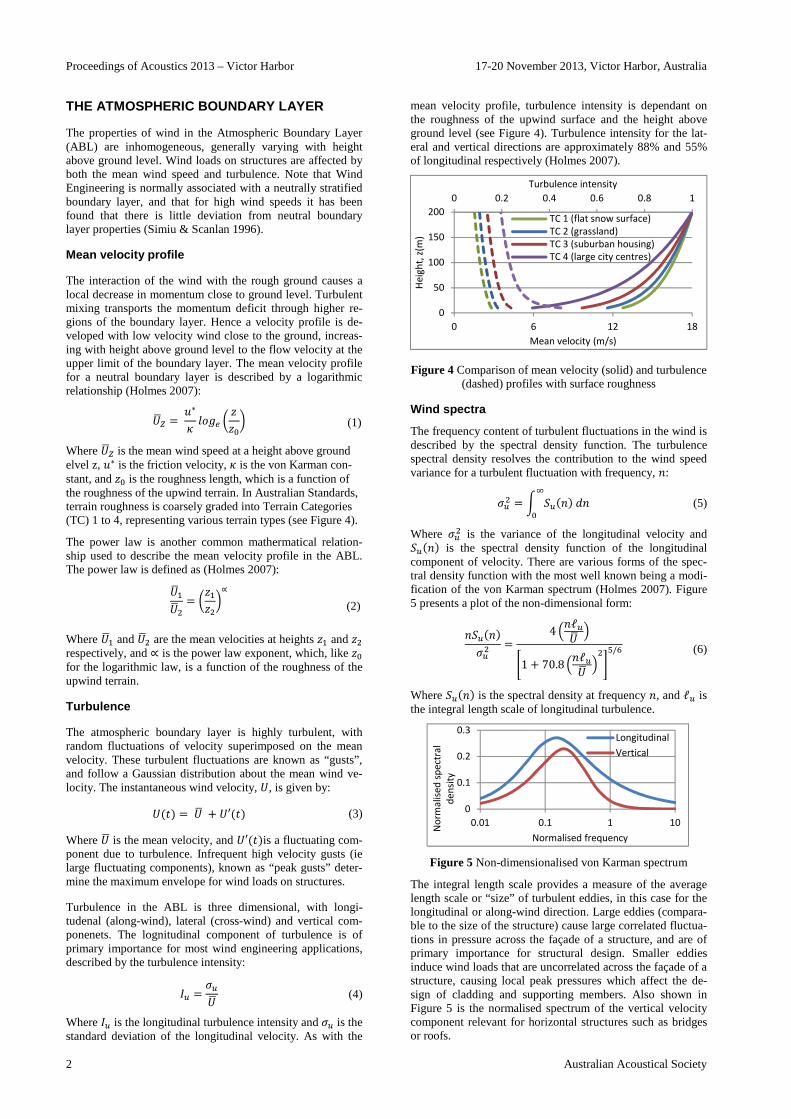
Where �� is the mean wind speed at a height above ground elvel z, �∗ is the friction velocity, � is the von Karman con-stant, and �� is the roughness length, which is a function of the roughness of the upwind terrain. In Australian Standards, terrain roughness is coarsely graded into Terrain Categories (TC) 1 to 4, representing various terrain types (see Figure 4).

The power law is another common mathermatical relation-ship used to describe the mean velocity profile in the ABL. The power law is defined as (Holmes 2007):

�� = ��

∝ (2)

Where �� and �� are the mean velocities at heights �� and �� respectively, and ∝ is the power law exponent, which, like �� for the logarithmic law, is a function of the roughness of the upwind terrain.

Turbulence

The atmospheric boundary layer is highly turbulent, with random fluctuations of velocity superimposed on the mean velocity. These turbulent fluctuations are known as “gusts”, and follow a Gaussian distribution about the mean wind ve-locity. The instantaneous wind velocity, �, is given by:

�(�) = �� + �′(�) (3)

Where �� is the mean velocity, and �′(�)is a fluctuating com-ponent due to turbulence. Infrequent high velocity gusts (ie large fluctuating components), known as “peak gusts” deter-mine the maximum envelope for wind loads on structures.

Turbulence in the ABL is three dimensional, with longi-tudenal (along-wind), lateral (cross-wind) and vertical com-ponenets. The lognitudinal component of turbulence is of primary importance for most wind engineering applications, described by the turbulence intensity:

�� = �� (4)

Where �� is the longitudinal turbulence intensity and �� is the standard deviation of the longitudinal velocity. As with the

mean velocity profile, turbulence intensity is dependant on the roughness of the upwind surface and the height above ground level (see Figure 4). Turbulence intensity for the lat-eral and vertical directions are approximately 88% and 55% of longitudinal respectively (Holmes 2007).

Figure 4 Comparison of mean velocity (solid) and turbulence (dashed) profiles with surface roughness

Wind spectra

The frequency content of turbulent fluctuations in the wind is described by the spectral density function. The turbulence spectral density resolves the contribution to the wind speed variance for a turbulent fluctuation with frequency, �:

�� = � ��(�)�� (5)

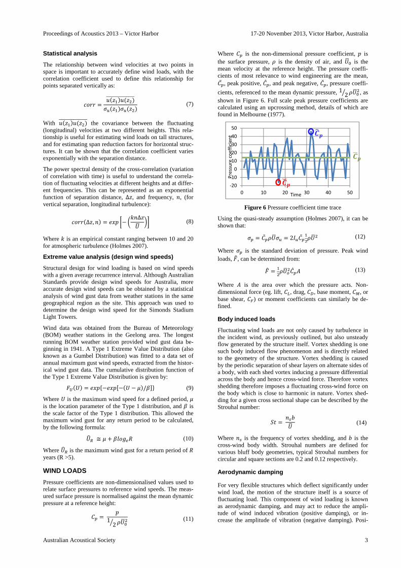
Where �� is the variance of the longitudinal velocity and ��(�) is the spectral density function of the longitudinal component of velocity. There are various forms of the spec-tral density function with the most well known being a modi-fication of the von Karman spectrum (Holmes 2007). Figure 5 presents a plot of the non-dimensional form:

��(�)�� = 4"�ℓ�� $%1 + 70.8 "�ℓ�� $

�+,/. (6)

Where ��(�) is the spectral density at frequency �, and ℓ� is the integral length scale of longitudinal turbulence.

Figure 5 Non-dimensionalised von Karman spectrum

The integral length scale provides a measure of the average length scale or “size” of turbulent eddies, in this case for the longitudinal or along-wind direction. Large eddies (compara-ble to the size of the structure) cause large correlated fluctua-tions in pressure across the façade of a structure, and are of primary importance for structural design. Smaller eddies induce wind loads that are uncorrelated across the façade of a structure, causing local peak pressures which affect the de-sign of cladding and supporting members. Also shown in Figure 5 is the normalised spectrum of the vertical velocity component relevant for horizontal structures such as bridges or roofs.

0 0.2 0.4 0.6 0.8 1

0

50

100

150

200

0 6 12 18

Turbulence intensity

He

igh

t, z

(m)

Mean velocity (m/s)

TC 1 (flat snow surface)

TC 2 (grassland)

TC 3 (suburban housing)

TC 4 (large city centres)

0

0.1

0.2

0.3

0.01 0.1 1 10

No

rma

lise

d s

pe

ctra

l

de

nsi

ty

Normalised frequency

Longitudinal

Vertical



Statistical analysis

The relationship between wind velocities at two points in space is important to accurately define wind loads, with the correlation coefficient used to define this relationship for points separated vertically as:

/00 = �(��)�(��)11111111111111��(��)��(��) (7)

With �(��)�(��)11111111111111 the covariance between the fluctuating (longitudinal) velocities at two different heights. This rela-tionship is useful for estimating wind loads on tall structures, and for estimating span reduction factors for horizontal struc-tures. It can be shown that the correlation coefficient varies exponentially with the separation distance.

The power spectral density of the cross-correlation (variation of correlation with time) is useful to understand the correla-tion of fluctuating velocities at different heights and at differ-ent frequencies. This can be represented as an exponential function of separation distance, Δ�, and frequency, �, (for vertical separation, longitudinal turbulence):

/00(Δ�, �) = 456 7− 9�Δ�� : (8)

Where 9 is an empirical constant ranging between 10 and 20 for atmospheric turbulence (Holmes 2007).

Extreme value analysis (design wind speeds)

Structural design for wind loading is based on wind speeds with a given average recurrence interval. Although Australian Standards provide design wind speeds for Australia, more accurate design wind speeds can be obtained by a statistical analysis of wind gust data from weather stations in the same geographical region as the site. This approach was used to determine the design wind speed for the Simonds Stadium Light Towers.

Wind data was obtained from the Bureau of Meteorology (BOM) weather stations in the Geelong area. The longest running BOM weather station provided wind gust data be-ginning in 1941. A Type 1 Extreme Value Distribution (also known as a Gumbel Distribution) was fitted to a data set of annual maximum gust wind speeds, extracted from the histor-ical wind gust data. The cumulative distribution function of the Type 1 Extreme Value Distribution is given by:

;<(�) = 456=−456>−(� − ?)/@AB (9)

Where � is the maximum wind speed for a defined period, ? is the location parameter of the Type 1 distribution, and @ is the scale factor of the Type 1 distribution. This allowed the maximum wind gust for any return period to be calculated, by the following formula:

�CD ≅ ? + @��F (10)

Where �CD is the maximum wind gust for a return period of F years (R >5).

WIND LOADS

Pressure coefficients are non-dimensionalised values used to relate surface pressures to reference wind speeds. The meas-ured surface pressure is normalised against the mean dynamic pressure at a reference height:

GH = 61 2J K�� (11)

Where GH is the non-dimensional pressure coefficient, 6 is the surface pressure, K is the density of air, and �� is the mean velocity at the reference height. The pressure coeffi-cients of most relevance to wind engineering are the mean, GH̅, peak positive, GMH, and peak negative, GNH, pressure coeffi-

cients, referenced to the mean dynamic pressure, 1 2J K��, as shown in Figure 6. Full scale peak pressure coefficients are calculated using an upcrossing method, details of which are found in Melbourne (1977).

Figure 6 Pressure coefficient time trace

Using the quasi-steady assumption (Holmes 2007), it can be shown that:

�H = GH̅K�� = 2��GH̅��K�� (12)

Where �H is the standard deviation of pressure. Peak wind loads, ;O, can be determined from:

;O = ��K��P�GMHQ (13)

Where Q is the area over which the pressure acts. Non-dimensional force (eg. lift, GR, drag, GS, base moment, GT, or base shear, GU) or moment coefficients can similarly be de-fined.

Body induced loads

Fluctuating wind loads are not only caused by turbulence in the incident wind, as previously outlined, but also unsteady flow generated by the structure itself. Vortex shedding is one such body induced flow phenomenon and is directly related to the geometry of the structure. Vortex shedding is caused by the periodic separation of shear layers on alternate sides of a body, with each shed vortex inducing a pressure differential across the body and hence cross-wind force. Therefore vortex shedding therefore imposes a fluctuating cross-wind force on the body which is close to harmonic in nature. Vortex shed-ding for a given cross sectional shape can be described by the Strouhal number:

�� = �VW�� (14)

Where �V is the frequency of vortex shedding, and W is the cross-wind body width. Strouhal numbers are defined for various bluff body geometries, typical Strouhal numbers for circular and square sections are 0.2 and 0.12 respectively.

Aerodynamic damping

For very flexible structures which deflect significantly under wind load, the motion of the structure itself is a source of fluctuating load. This component of wind loading is known as aerodynamic damping, and may act to reduce the ampli-tude of wind induced vibration (positive damping), or in-crease the amplitude of vibration (negative damping). Posi-

-20

-10

0

10

20

30

40

50

0 10 20 30 40 50

Pre

ssu

re c

oe

ffic

ien

t

Time

X�Y

XCY

XZY



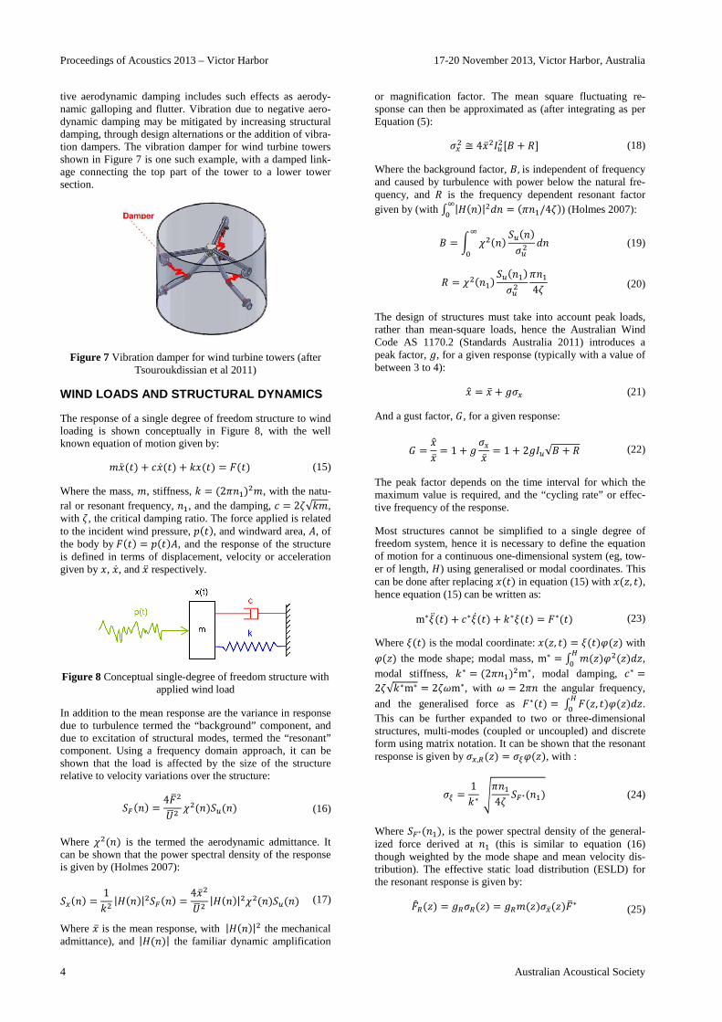
tive aerodynamic damping includes such effects as aerody-namic galloping and flutter. Vibration due to negative aero-dynamic damping may be mitigated by increasing structural damping, through design alternations or the addition of vibra-tion dampers. The vibration damper for wind turbine towers shown in Figure 7 is one such example, with a damped link-age connecting the top part of the tower to a lower tower section.

Figure 7 Vibration damper for wind turbine towers (after Tsouroukdissian et al 2011)

WIND LOADS AND STRUCTURAL DYNAMICS

The response of a single degree of freedom structure to wind loading is shown conceptually in Figure 8, with the well known equation of motion given by:

[5\(�) + /5](�) + 95(�) = ;(�) (15)

Where the mass, [, stiffness, 9 = (2^��)�[, with the natu-ral or resonant frequency, ��, and the damping, / = 2_√9[, with _, the critical damping ratio. The force applied is related to the incident wind pressure, 6(�), and windward area, Q, of the body by;(�) = 6(�)Q, and the response of the structure is defined in terms of displacement, velocity or acceleration given by 5, 5] , and 5\ respectively.

Figure 8 Conceptual single-degree of freedom structure with applied wind load

In addition to the mean response are the variance in response due to turbulence termed the “background” component, and due to excitation of structural modes, termed the “resonant” component. Using a frequency domain approach, it can be shown that the load is affected by the size of the structure relative to velocity variations over the structure:

�U(�) = 4;1�� a�(�)��(�) (16)

Where a�(�) is the termed the aerodynamic admittance. It can be shown that the power spectral density of the response is given by (Holmes 2007):

�b(�) = 19� |d(�)|��U(�) = 45̅�

�� |d(�)|�a�(�)��(�) (17)

Where 5̅ is the mean response, with |d(�)|� the mechanical admittance), and |d(�)| the familiar dynamic amplification

or magnification factor. The mean square fluctuating re-sponse can then be approximated as (after integrating as per Equation (5):

�b� ≅ 45̅��>e + FA (18)

Where the background factor, e,is independent of frequency and caused by turbulence with power below the natural fre-quency, and F is the frequency dependent resonant factor given by (with f |d(�)|�� = (^��/4_) � ) (Holmes 2007):

e = � a�(�) ��(�)�� (19)

F = a�(��) ��(��)��^��4_ (20)

The design of structures must take into account peak loads, rather than mean-square loads, hence the Australian Wind Code AS 1170.2 (Standards Australia 2011) introduces a peak factor, �, for a given response (typically with a value of between 3 to 4):

5g = 5̅ + ��b (21)

And a gust factor, h, for a given response:

h = 5g5̅ = 1 + � �b5̅ = 1 + 2��√e + F (22)

The peak factor depends on the time interval for which the maximum value is required, and the “cycling rate” or effec-tive frequency of the response.

Most structures cannot be simplified to a single degree of freedom system, hence it is necessary to define the equation of motion for a continuous one-dimensional system (eg, tow-er of length, d) using generalised or modal coordinates. This can be done after replacing 5(�) in equation (15) with 5(�, �), hence equation (15) can be written as:

m∗j\(�) + /∗j](�) + 9∗j(�) = ;∗(�) (23)

Where j(�) is the modal coordinate: 5(�, �) = j(�)k(�) with k(�) the mode shape; modal mass, m∗ = f [(�)k�(�)��l� , modal stiffness, 9∗ = (2^��)�m∗, modal damping, /∗ =2_√9∗m∗ = 2_mm∗, with m = 2^� the angular frequency,

and the generalised force as ;∗(�) = f ;(�, �)k(�)��l� . This can be further expanded to two or three-dimensional structures, multi-modes (coupled or uncoupled) and discrete form using matrix notation. It can be shown that the resonant response is given by �b,D(�) = �nk(�), with :

�n = 19∗ o^��4_ �U∗(��) (24)

Where �U∗(��), is the power spectral density of the general-ized force derived at �� (this is similar to equation (16) though weighted by the mode shape and mean velocity dis-tribution). The effective static load distribution (ESLD) for the resonant response is given by:

;OD(�) = �D�D(�) = �D[(�)�b\(�);1∗ (25)



Where �D and �D are the peak factor and standard deviation for the resonant component respectively, and �b\(�) =m��b(�) is the RMS acceleration. The ESLD for the back-ground response can be calculated using a time domain ap-proach, as shown by Kasperski and Niemann (1992):

;Op(�) = �p�p(�) = �pK(�)�H(�) (26)

Where �p is the peak factor for the background component, K(�) is the correlation coefficient between the fluctuating load at point � on the structure and the load effect of interest, and �H(�) was defined earlier (equation (12)). Finally, the ESLD for the mean response is given by:

;1(�) = ��K��(�)GH̅(�)W(�) (27)

Where GH̅(�) is the mean pressure coefficient, and W(�) is the width of the structure at height �. These components can be combined as:

;O(�) = ;1(�) + q;Op�(�) + ;OD�(�) (28)

WIND TUNNEL TEST METHODS

Wind engineering wind tunnel tests involve placing an in-strumented physical scale model of the development of inter-est in similarly scaled wind. Measurements for the Simonds Stadium Light Tower and Adelaide Oval were carried out using the atmospheric boundary layer wind tunnel at the Uni-versity of Sydney. This tunnel has a cross-section of 4.5 m2, a turntable of diameter 2.3 m and a boundary layer develop-ment length of 15 m.

ABL simulation

The minimum requirements for an acceptable simulation of a neutrally stable atmospheric boundary layer are the modeling of: • The variation of mean wind speed with height, • The variation of longitudinal component of turbulence

with height, • The integral scale of turbulence, • A zero longitudinal pressure gradient (achieved through

the used of a slotted ceilings or open test section) (AWES 2001).

Wind tunnel flow conditioning devices were used to create a scaled boundary layer with velocity and turbulence character-istics appropriate for the terrain category of the upwind ter-rain. The flow conditioning devices included a trip board, spires and roughness elements positioned over the develop-ment length of the wind tunnel.

Near-field flow

Nearby structures or topographical features influence the near field flow and are included as part of the wind tunnel model. All major structures and topographical features within a radi-us of a few hundred metres of the building site are modeled to the correct scale.

Model-prototype similarity

The fundamental concept of wind tunnel testing is that the model and the wind should be at approximately the same scale. Geometric scale is important, as it determines the size of the model and calibration of the wind; however appropri-

ate velocity, time and frequency scales are also neccesary for instrumentation sampling and frequency response character-istics.

The Reynolds number denotes the ratio of inertial forces to viscous forces, and is of particular significance to develop-ments featuring elements of circular cross section. Reynolds number greatly affects drag for these elements and approxi-mate Reynolds number similarity is required during wind tunnel testing. For most developments, it is sufficient to meet a minimum Reynolds number due to difficulties meeting the prototype Reynolds number at model scale.

Measurement methods

High frequency base balance

Measurements of base forces and moments are made using a lightweight stiff model with a high natural frequency, typical-ly constructed of acrylic or lightweight wood. The model is mounted on a six degree of freedom high frequency base balance (HFBB) and is otherwise mechanically isolated from the rest of the wind tunnel. Strain gauges in the HFBB sense the imposed wind loads, with the strain gauge signals ampli-fied and combined into analog representations of the forces and moments about the 3 axes. The dynamic properties of the stiff model ensure that the base loads will not be influenced by resonance of the scale model.

Pressure taps

Scale models required for pressure measurement are typically constructed from acrylic using traditional model making techinques, and plastic resin using rapid protyping techniques (eg stereolithography, laser sintering). Surface pressure measurements on the model are made using pressure taps, which are connected via tubing to pressure transducers. The transducers convert the measured pressure to an electrical signal which is then digitised and adjusted by a calibration factor.

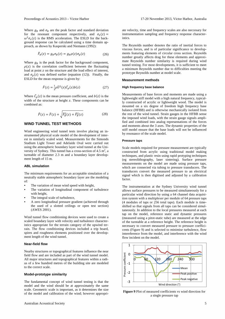
The instrumentation at the Sydney University wind tunnel allows surface pressures to be measured simultaneously for a particular wind direction by using a 64 channel data acquisi-tion system with a multiplexer per module of 64 pressure taps (4 modules of taps or 256 total taps). Each module is time-shifted so that signals from all taps can be considered simul-taneously. In addition to the local pressures measured at each tap on the model, reference static and dynamic pressures (measured using a pitot-static tube) are measured at the edge of the turntable at a reference height. The reference height is necessary to convert measured pressure to pressure coeffici-cents (Figure 9) and is selected to minimise turbulence, flow intereference from the model, and interference with the wind flow incident on the model.

Figure 9 Plot of measured coefficients vs wind direction for a single pressure tap

-3

-2

-1

0

1

0 60 120 180 240 300

Pre

ssu

re c

oe

ffic

ien

t

Wind direction (°)

Mean

Peak positive

Peak negative



SIMONDS STADIUM LIGHT TOWERS

Site extreme wind speed

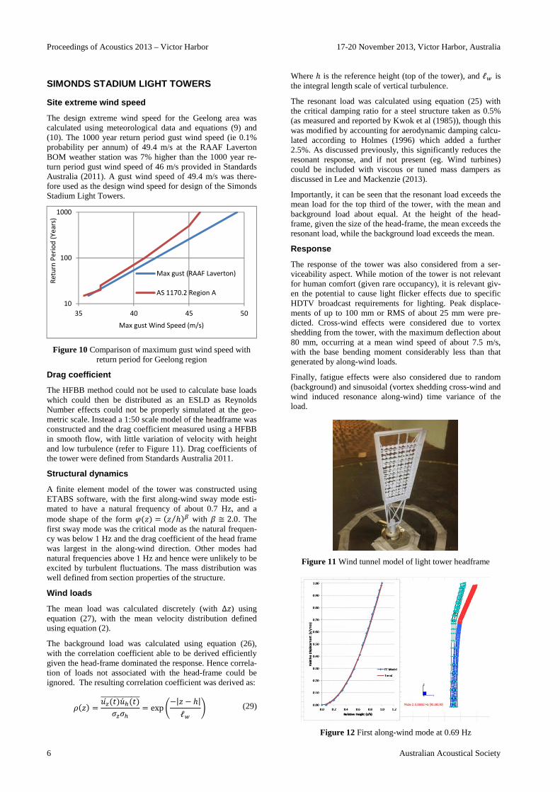
The design extreme wind speed for the Geelong area was calculated using meteorological data and equations (9) and (10). The 1000 year return period gust wind speed (ie 0.1% probability per annum) of 49.4 m/s at the RAAF Laverton BOM weather station was 7% higher than the 1000 year re-turn period gust wind speed of 46 m/s provided in Standards Australia (2011). A gust wind speed of 49.4 m/s was there-fore used as the design wind speed for design of the Simonds Stadium Light Towers.

Figure 10 Comparison of maximum gust wind speed with

return period for Geelong region

Drag coefficient

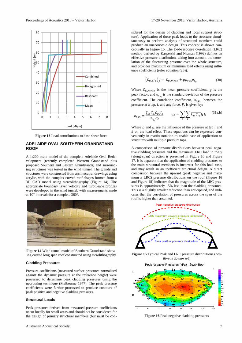
The HFBB method could not be used to calculate base loads which could then be distributed as an ESLD as Reynolds Number effects could not be properly simulated at the geo-metric scale. Instead a 1:50 scale model of the headframe was constructed and the drag coefficient measured using a HFBB in smooth flow, with little variation of velocity with height and low turbulence (refer to Figure 11). Drag coefficients of the tower were defined from Standards Australia 2011.

Structural dynamics

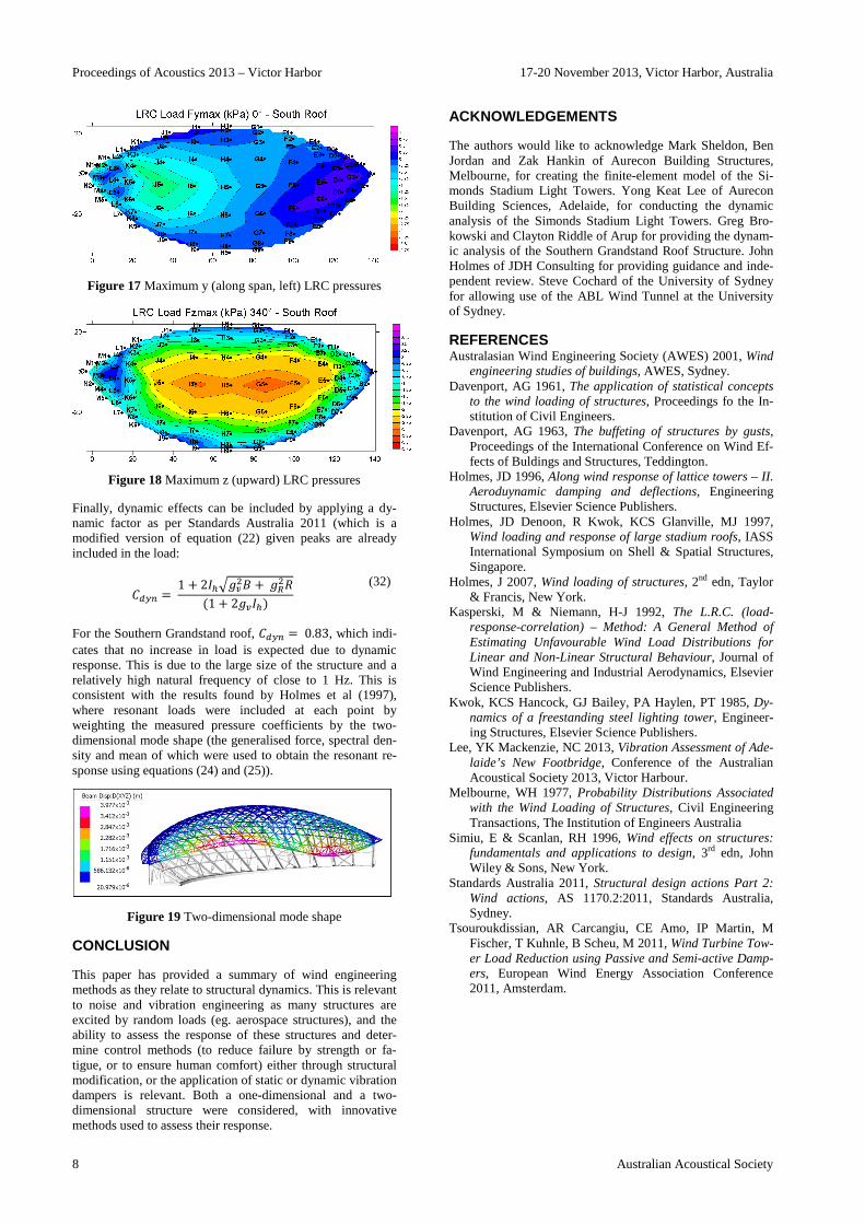
A finite element model of the tower was constructed using ETABS software, with the first along-wind sway mode esti-mated to have a natural frequency of about 0.7 Hz, and a mode shape of the form k(�) = (� r⁄ )t with @ ≅ 2.0. The first sway mode was the critical mode as the natural frequen-cy was below 1 Hz and the drag coefficient of the head frame was largest in the along-wind direction. Other modes had natural frequencies above 1 Hz and hence were unlikely to be excited by turbulent fluctuations. The mass distribution was well defined from section properties of the structure.

Wind loads

The mean load was calculated discretely (with ∆�) using equation (27), with the mean velocity distribution defined using equation (2).

The background load was calculated using equation (26), with the correlation coefficient able to be derived efficiently given the head-frame dominated the response. Hence correla-tion of loads not associated with the head-frame could be ignored. The resulting correlation coefficient was derived as:

K(�) = �v́(�)�́x(�)11111111111111�v�x = exp|−|� − r|ℓ} ~ (29)

Where r is the reference height (top of the tower), and ℓ} is the integral length scale of vertical turbulence.

The resonant load was calculated using equation (25) with the critical damping ratio for a steel structure taken as 0.5% (as measured and reported by Kwok et al (1985)), though this was modified by accounting for aerodynamic damping calcu-lated according to Holmes (1996) which added a further 2.5%. As discussed previously, this significantly reduces the resonant response, and if not present (eg. Wind turbines) could be included with viscous or tuned mass dampers as discussed in Lee and Mackenzie (2013).

Importantly, it can be seen that the resonant load exceeds the mean load for the top third of the tower, with the mean and background load about equal. At the height of the head-frame, given the size of the head-frame, the mean exceeds the resonant load, while the background load exceeds the mean.

Response

The response of the tower was also considered from a ser-viceability aspect. While motion of the tower is not relevant for human comfort (given rare occupancy), it is relevant giv-en the potential to cause light flicker effects due to specific HDTV broadcast requirements for lighting. Peak displace-ments of up to 100 mm or RMS of about 25 mm were pre-dicted. Cross-wind effects were considered due to vortex shedding from the tower, with the maximum deflection about 80 mm, occurring at a mean wind speed of about 7.5 m/s, with the base bending moment considerably less than that generated by along-wind loads.

Finally, fatigue effects were also considered due to random (background) and sinusoidal (vortex shedding cross-wind and wind induced resonance along-wind) time variance of the load.

Figure 11 Wind tunnel model of light tower headframe

Figure 12 First along-wind mode at 0.69 Hz

10

100

1000

35 40 45 50

Re

turn

Pe

rio

d (

Ye

ars

)

Max gust Wind Speed (m/s)

Max gust (RAAF Laverton)

AS 1170.2 Region A



Figure 13 Load contributions to base shear force

ADELAIDE OVAL SOUTHERN GRANDSTAND ROOF

A 1:200 scale model of the complete Adelaide Oval Rede-velopment (recently completed Western Grandstand plus proposed Southern and Eastern Grandstands) and surround-ing structures was tested in the wind tunnel. The grandstand structures were constructed from architecutral drawings using acrylic, with the complex curved roof shapes formed from a 3D CAD model using stereolithography (Figure 14). The appropriate boundary layer velocity and turbulence profiles were developed in the wind tunnel, with measurements made at 10° intervals for a complete 360°.

Figure 14 Wind tunnel model of Southern Grandstand show-ing curved long span roof constructed using sterolithography

Cladding Pressures

Pressure coefficients (measured surface pressures normalised against the dynamic pressure at the reference height) were processed to determine peak cladding pressures using the upcrossing technique (Melbourne 1977). The peak pressure coefficients were further processed to produce contours of peak positive and negative cladding pressures.

Structural Loads

Peak pressures derived from measured pressure coefficients occur locally for small areas and should not be considered for the design of primary structural members (but must be con-

sidered for the design of cladding and local support struc-ture). Application of these peak loads to the structure simul-taneously to perform analysis of structural members could produce an uneconomic design. This concept is shown con-ceptually in Figure 15. The load-response correlation (LRC) method derived by Kasperski and Nieman (1992) defines an effective pressure distribution, taking into account the corre-lation of the fluctuating pressure over the whole structure, and provides maximum or minimum load effects using influ-ence coefficients (refer equation (26)):

�GH�,��UO = GH�,�� ± �KU,H�� (30)

Where GH�,�� is the mean pressure coefficient, � is the peak factor, and �� is the standard deviation of the pressure

coefficient. The correlation coefficient, KU,H� , between the pressure at a tap, �, and any force, ;, is given by:

KU,H� = ∑ GH�GH�11111111��U �U =��GH�GH�11111111�� (31a,b)

Where �� and �� are the influence of the pressure at tap � and 9 on the load effect. These equations can be expressed con-veniently in matrix notation to enable ease of application to structures with multiple pressure taps.

A comparison of pressure distributions between peak nega-tive cladding pressures and the maximum LRC load in the y (along span) direction is presented in Figure 16 and Figure 17. It is apparent that the application of cladding pressures to the main structural members is incorrect for this load case, and may result in an inefficient structural design. A direct comparison between the upward (peak negative and maxi-mum z LRC) pressure distributions on the roof (Figure 16 and Figure 18) indicates that the magnitude of the LRC pres-sures is approximately 15% less than the cladding pressures. This is a slightly smaller reduction than anticipated, and indi-cates that the correlation of pressures across the span of the roof is higher than assumed.

Figure 15 Typical Peak and LRC pressure distributions (pos-itive is downward)

Figure 16 Peak negative cladding pressures

0

10

20

30

40

50

60

70

80

0 1 2 3 4 5 6 7 8

He

igh

t (m

)

Load (kN/m)

Combined

Background

Resonant

Mean



Figure 17 Maximum y (along span, left) LRC pressures

Figure 18 Maximum z (upward) LRC pressures

Finally, dynamic effects can be included by applying a dy-namic factor as per Standards Australia 2011 (which is a modified version of equation (22) given peaks are already included in the load:

G�� =1 + 2�x��e +�D�F(1 + 2��x) (32)

For the Southern Grandstand roof, G�� = 0.83, which indi-cates that no increase in load is expected due to dynamic response. This is due to the large size of the structure and a relatively high natural frequency of close to 1 Hz. This is consistent with the results found by Holmes et al (1997), where resonant loads were included at each point by weighting the measured pressure coefficients by the two-dimensional mode shape (the generalised force, spectral den-sity and mean of which were used to obtain the resonant re-sponse using equations (24) and (25)).

Figure 19 Two-dimensional mode shape

CONCLUSION

This paper has provided a summary of wind engineering methods as they relate to structural dynamics. This is relevant to noise and vibration engineering as many structures are excited by random loads (eg. aerospace structures), and the ability to assess the response of these structures and deter-mine control methods (to reduce failure by strength or fa-tigue, or to ensure human comfort) either through structural modification, or the application of static or dynamic vibration dampers is relevant. Both a one-dimensional and a two-dimensional structure were considered, with innovative methods used to assess their response.

ACKNOWLEDGEMENTS

The authors would like to acknowledge Mark Sheldon, Ben Jordan and Zak Hankin of Aurecon Building Structures, Melbourne, for creating the finite-element model of the Si-monds Stadium Light Towers. Yong Keat Lee of Aurecon Building Sciences, Adelaide, for conducting the dynamic analysis of the Simonds Stadium Light Towers. Greg Bro-kowski and Clayton Riddle of Arup for providing the dynam-ic analysis of the Southern Grandstand Roof Structure. John Holmes of JDH Consulting for providing guidance and inde-pendent review. Steve Cochard of the University of Sydney for allowing use of the ABL Wind Tunnel at the University of Sydney.

REFERENCES Australasian Wind Engineering Society (AWES) 2001, Wind

engineering studies of buildings, AWES, Sydney. Davenport, AG 1961, The application of statistical concepts

to the wind loading of structures, Proceedings fo the In-stitution of Civil Engineers.

Davenport, AG 1963, The buffeting of structures by gusts, Proceedings of the International Conference on Wind Ef-fects of Buldings and Structures, Teddington.

Holmes, JD 1996, Along wind response of lattice towers – II. Aeroduynamic damping and deflections, Engineering Structures, Elsevier Science Publishers.

Holmes, JD Denoon, R Kwok, KCS Glanville, MJ 1997, Wind loading and response of large stadium roofs, IASS International Symposium on Shell & Spatial Structures, Singapore.

Holmes, J 2007, Wind loading of structures, 2nd edn, Taylor & Francis, New York.

Kasperski, M & Niemann, H-J 1992, The L.R.C. (load-response-correlation) – Method: A General Method of Estimating Unfavourable Wind Load Distributions for Linear and Non-Linear Structural Behaviour, Journal of Wind Engineering and Industrial Aerodynamics, Elsevier Science Publishers.

Kwok, KCS Hancock, GJ Bailey, PA Haylen, PT 1985, Dy-namics of a freestanding steel lighting tower, Engineer-ing Structures, Elsevier Science Publishers.

Lee, YK Mackenzie, NC 2013, Vibration Assessment of Ade-laide’s New Footbridge, Conference of the Australian Acoustical Society 2013, Victor Harbour.

Melbourne, WH 1977, Probability Distributions Associated with the Wind Loading of Structures, Civil Engineering Transactions, The Institution of Engineers Australia

Simiu, E & Scanlan, RH 1996, Wind effects on structures: fundamentals and applications to design, 3rd edn, John Wiley & Sons, New York.

Standards Australia 2011, Structural design actions Part 2: Wind actions, AS 1170.2:2011, Standards Australia, Sydney.

Tsouroukdissian, AR Carcangiu, CE Amo, IP Martin, M Fischer, T Kuhnle, B Scheu, M 2011, Wind Turbine Tow-er Load Reduction using Passive and Semi-active Damp-ers, European Wind Energy Association Conference 2011, Amsterdam.

dynamic assessment of wind sensitive stadium · pdf filedynamic assessment of wind sensitive...

Documents