dynamic and efficiency characteristics of an inlet
TRANSCRIPT

DYNAMIC AND EFFICIENCY CHARACTERISTICS OF AN INLET METERING VALVE
CONTROLLED FIXED DISPLACEMENT PUMP
_______________________________________
A Dissertation
presented to
the Faculty of the Graduate School
at the University of Missouri-Columbia
_______________________________________________________
In Partial Fulfillment
of the Requirements for the Degree
Doctor of Philosophy
_____________________________________________________
by
Julie Kay Wisch
Dr. Noah D. Manring, Dissertation Adviser
MAY 2016

The undersigned, appointed by the dean of the Graduate School, have examined the dissertation
entitled
DYNAMIC AND EFFICIENCY CHARACTERISTICS OF AN INLET METERING VALVE
CONTROLLED FIXED DISPLACEMENT PUMP
presented by Julie Wisch,
a candidate for the degree of doctor of philosophy, and hereby certify that, in their opinion, it is
worthy of acceptance.
Professor Noah Manring
Professor Roger Fales
Professor Gary Solbrekken
Professor Jacob McFarland
Professor Steve Borgelt

ii
ACKNOWLEDGEMENTS
I would like to thank my committee: Roger Fales, Gary Solbrekken, Jacob
McFarland, and Steve Borgelt for their support in this endeavor. I would most especially
like to thank Noah Manring, who has worked with me throughout this project, and
devoted considerable time and attention to critically reviewing my work and pointing me
in the right direction.
I would also like to thank our partners at Caterpillar: Jeff Kuehn, Jeremy
Peterson, Viral Mehta, Hongliu Du, and Randy Harlow for both the financial support and
collective engineering experience that they contributed to this project. I am lucky to have
had a team of engineers to brainstorm with, and am so grateful for the prototype they
were able to provide.
Thank you to Dr. Frank Feng, who was both an excellent mentor for my time as a
teaching assistant, as well as the person who introduced me to another funding
opportunity for my graduate studies via the Missouri Space Grant Consortium. Thank
you to Doug Steinhoff, Karen King, Leon Schumacher, and Steve Borgelt who all
facilitated opportunities for me to explore teaching and develop skills in that area.
Finally, I would like to thank my parents, Kevin and Karen Wisch. They always
show up for me, and I couldn’t ask for anything more.

iii
TABLE OF CONTENTS
ACKNOWLEDGEMENTS ................................................................................................ ii
LIST OF FIGURES .............................................................................................................v
LIST OF TABLES ............................................................................................................ vii
NOMENCLATURE ........................................................................................................ viii
CHAPTER
1. INTRODUCTION ..........................................................................................1
Background and Motivation
System Description
Experimental Set Up
Contribution
Dissertation Outline
2. LITERATURE REVIEW .............................................................................11
Literature Review Introduction
Inlet Metering Valves
Hydraulic Systems, A Brief History
A Comparison of Oil and Water Hydraulic Systems
Cavitation
Machine Design Considerations
Entrained Air
Fluid Modeling Justification
Literature Conclusions
3. ANALYSIS ...................................................................................................26
Analysis Introduction
Transient Pressure Analysis
Pump Discharge Flow
Pump Flow Phase I
Pump Flow Phase II
Pump Flow Phase III
Pump Flow Phase IV
Pump Flow Summary
Inlet Metering Valve
Valve Flow Force Considerations
Flow Force Analysis
Full Dynamic Valve Equation
Summary of Dimensional Equations
Nondimensionalization
Variable Displacement Pump Model

iv
4. EFFICIENCY ...............................................................................................50
Efficiency Introduction
Traditional Pump Efficiency
Inlet Metering Pump Efficiency
Efficiency Model Validation
Discussion of the Variable Displacement and Inlet Metering System
5. DESIGN AND MODELING ........................................................................72
Introduction to System Design and Modeling
System Stability
Design Criteria Development
Solution of the System of Equations
Dynamic System Response
Design Process
Illustrative Model Selection
Modeling Introduction
6. RESULTS AND DISCUSSION ...................................................................89
Results Introduction
Experimental Results
System Efficiency Results
Valve and Pressure Response Results
Stability Discussion
Design Parameter Adherence
A Qualitative Discussion about the Inlet Metering System Efficiency
System Dynamics Comparison
Discussion of Valve Dynamic System Response
7. CONCLUSION ...........................................................................................119
Conclusion Introduction
List of Conclusions
Comparative Analysis
Future Work
REFERENCES ................................................................................................................128
APPENDIX ......................................................................................................................137
VITA ................................................................................................................................148
v
LIST OF FIGURES
Figure Page
1-1. System design and associated nomenclature ...........................................................3
1-2. Spool valve...............................................................................................................4
1-3. Piston pump ............................................................................................................5
1-4. Test rig experimental set up ....................................................................................7
2-1. Diesel fuel injector diagram .................................................................................12
3-1. Piston pump ..........................................................................................................27
3-2. Strip chart illustrating piston pressure and displacement .....................................28
3-3. Inlet metering valve and associated nomenclature ...............................................37
3-4. Inlet metering valve free body diagram ................................................................41
3-5. Inlet metering valve flow at the outlet ..................................................................42
4-1. Variable displacement pump diagram ..................................................................51
4-2. Schematic of the pump, showing mass and volumetric flow rates .......................52
4-3. Inlet metering system control volume definition ..................................................57
4-4. Pressure as a Function of Crankshaft Position .....................................................58
4-5. Levenberg-Marquardt Solution Process ...............................................................67
5-1. Block diagram of the full order inlet metering valve system ...............................87
5-2. Block diagram of the reduced order inlet metering valve system ........................88
6-1. Inlet Metering System Experimental Set Up .........................................................90
6-2. Volumetric flow rate over time ............................................................................91
6-3. Averaged nondimensional discharge flow per position .......................................92
6-4. Averaged nondimensional discharge flow per position ........................................94
6-5. Averaged nondimensional discharge flow per position ........................................95
6-6. Comparison of fluid flow to valve position ...........................................................99
6-7. Torque requirement ............................................................................................100
6-8. Pump efficiency as a function of pump flow output ..........................................101
6-9. Inlet metering pump efficiency map ....................................................................102
6-10. Measured efficiency results for the inlet metering system ..................................103
6-11. Normalized Efficiency Comparison ....................................................................105
6-12. Normalized Efficiency Discrepancy ....................................................................106
6-13. Models A and A’ valve displacement ..................................................................108
6-14. Models A and A’ discharge pressure behavior ....................................................108
6-15. Models B and B’ valve displacement ..................................................................109
6-16. Models B and B’ discharge pressure behavior ....................................................109
6-17. Model A valve displacement over an extended time period ...............................110
6-18. Model B valve displacement over an extended time period ................................111
6-19. Magnified view of Models B and B’ pressure response ......................................112
6-20. Models A and A’ Bode Plot ................................................................................114

vi
6-21. Models B and B’ Bode Plot .................................................................................114
6-22. Models A and A’ Step Response Plot .................................................................116
6-23. Models B and B’ Step Response Plot ..................................................................116
vii
LIST OF TABLES
Table Page
1-1. Experimental Conditions .........................................................................................8
2-1. Comparison of Fluid Power and Electric Power ...................................................13
3-1. Summary of pump flow behavior at throughout the cycle ....................................36
4-1. Pump coefficients for Eqs. (4.3) and (4.5) ...........................................................55
4-2. Summary of pump flow behavior throughout the cycle .......................................62
4-3. Inlet metering pump coefficients ..........................................................................68
4-4. Standard Deviation of Collected Data ..................................................................70
5-1. Design parameters ................................................................................................82
5-2. Model design parameter selections .......................................................................84
5-3. Numerical values associated with the nondimensional parameters in Eq. (3.52) 84
5-4. Models of interest and their associated dynamic characteristics ..........................85
6-1. Data Collection Points Associated with Experiments ..........................................90
6-2. Goodness of fit of predicted linear relationship as compared to experimental
data……………………………………………………………………………….96
6-3. Predicted fluid quality as a function of nondimensional flow and valve
position . …………………………………………………………………………97

viii
NOMENCLATURE
Square Cross-Sectional Area of the Valve Inlet
Rectangular Cross-Sectional Area of the Valve Outlet
Ap Static Friction Coefficient
pumpA Cross-Sectional Area of the Pump Inlet
Cross-Sectional Area of the Spool Valve
Nondimensional Cross-Sectional Valve Area
PB Boundary Lubrication Decay Rate Coefficient
c Viscous drag coefficient
Nondimensional Viscous Drag Coefficient
PC Hydrodynamic Lubrication Coefficient
Discharge Coefficient
Radial Clearance
Change in Volumetric Flow Rate as a Function of Time
PD Starting Torque Coefficient
E Specific Energy
e Error term in Levenberg-Marquardt process
Horizontal Flow Forces
Vertical Flow Forces
Initialized Spring Force
oA
A
VA
A
c
dc
dQ
dt
iF
jF
oF

ix
Pressure Induced Valve Force
Gravity
Enthalpy
J Jacobian Matrix
K Leakage Coefficient
0K Fluid Compression Coefficient
1K Low Reynolds Number Leakage
2K High Reynolds Number Leakage
Nondimensional Leakage Coefficient
Nondimensional Spring Rate Coefficient
k Valve Spring Constant
L Length of the Crankshaft
Mass of the Spool Valve
Mass Flow Rate
Nondimensional Valve Mass Coefficient
P Hydraulic Power
Pressure at the Valve Inlet
Pressure at the Valve Outlet
Pressure at the Pump Outlet
maxP Maximum System Operating Pressure
yF
g
h
1K
2K
vm
m
m
0P
1P
2P

x
Pressure in the Pump
Saturation Pressure of the Fluid
Steady State Pressure
Valve Inlet Volumetric Flow Rate
Pump Inlet Volumetric Flow Rate
Pump Outlet Volumetric Flow Rate
Volumetric Flow Rate Demand by the System
r Crank Radius
s Laplace Operator
T Torque on the Crankshaft
t Time
u Internal Energy
Nondimensional Specific Volume Ratio
Nondimensional Piston Volume Ratio
Pump Volume
Volumetric Displacement of the Pump
Liquid Specific Volume
Difference between Fluid Liquid Specific Volume and Fluid Vaporous Specific
Volume
Maximum Piston Internal Volume
Instantaneous Piston Internal Volume
PP
satP
ssP
0Q
1Q
2Q
sysQ
v
V
2V
dV
lv
lgv
maxV
nV

xi
w Weights in Levenberg-Marquardt solution process
Quality
y Spool Valve Displacement
Maximum Spool Valve Displacement
Steady State Valve Displacement
Vertical Position
Swashplate Angle
Fluid Bulk Modulus
Efficiency
Jet Angle, Crankshaft Displacement
Crankshaft Location
Time constant
0 Fluid Viscosity
Combination Coefficient
Nondimensional Fluid Property Group
Pump Shaft Speed
x
maxy
ssy
z

1
CHAPTER 1. INTRODUCTION
1.1 Background and Motivation
The body of this work applies some of the principles at work in a diesel fuel
injection system with a fixed displacement hydraulic pump in a way that creates a novel
approach to providing varied flow output. In the diesel fuel industry, “metering” refers to
the act of controlling the amount of fluid sprayed per charge [1]. For this work, an inlet
metering valve is installed upstream from a fixed displacement pump and is used to meter
the flow exiting the pump in a manner similar to the way diesel fuel injectors control the
amount of partially vaporized fuel injected into a diesel engine. A more thorough
examination of diesel fuel injection systems will be conducted in the literature review.
The inlet metering approach differs from traditional hydraulic pump flow rate
management. Pump flow is typically managed by one of three approaches: the shaft
speed of the pump is varied, the angle of the swashplate within a variable displacement
pump is varied, or a fixed displacement pump pushes a constant amount of flow and the
excess is simply dumped and recirculated in the system [2] (A detailed diagram of the
variable displacement pump is provided in Chapter 4). Fixed displacement pumps are
cheaper and more mechanically reliable than variable displacement pumps; however,
they contribute to large system inefficiencies since their excess flow is bypassed from
actual power supply. In aircraft gas turbine engines, for instance, the ratio of bypass flow
to engine flow can be up to twenty-fold [3]. Obviously this level of systemic inefficiency
is undesirable. This dissertation will attempt to use a fixed displacement pump but

2
minimize the losses that result from the bypass of excess flow and instead control the
flow at the pump outlet by means of an upstream inlet metering valve.
1.2 System Description
Figure 1-1 shows a schematic of the inlet metering system and the nomenclature
used throughout this paper. The inlet metering system is comprised of a charge pump, an
inlet metering valve, and a single piston pump which has check valves at both the inlet
and outlet. The fluid maintains an initial pressure and flow rate 0 0, P Q as established
by the charge pump. This pump will not receive further attention in the analysis in the
following pages; instead, it will be treated as a constant pressure reservoir upstream from
the inlet metering valve. The inlet metering valve is illustrated as a two-way spool valve
in Fig. 1-1.
The inlet metering valve serves as the control device for this system, and receives
considerable attention in the upcoming analysis. The typical operation of an inlet
metering valve can be observed in a diesel fuel injection system.
In a diesel fuel injector, diesel fuel is supplied to a throttling valve, which is
controlled by an electronic control device. The amount of fluid distributed is adjusted by
changing the orifice diameter of the fluid injector outlet [4]. As the pressure drop across
the orifice increases, an increasing percentage of the diesel fuel is vaporized. In diesel
fuel injection systems, poppet valves are commonly used [5]. However, for our design
purposes, the metering valve that will be modeled is a spool valve. Spool valves have
been found to better handle pressure oscillations [6]. Our primary design objective is to

3
Char
ge
Pum
p
Fig
ure
1-1
. S
yst
em D
esig
n a
nd A
ssoci
ated
Nom
encl
ature
Spool
Val
ve
Pis
ton P
um
p
Dow
nst
ream
Load

4
maintain a constant return pressure while the pump’s output flow demand varies. Thus,
the spool valve is well suited for our needs.
Figure 1-2. Spool Valve
The inlet metering valve is shown in Fig. 1-2. We will control the cross-sectional
area A of the spool valve and will subsequently maintain control over the pressure drop
across the valve. This pressure drop will induce partial vaporization of the working fluid.
The predicted phase change will occur as the fluid moves from the fluid supply (indicated
with a “0” subscript) into the contracted valve area (indicated with a “1” in the subscript).
The inlet metering valve (shown in Fig. 1-2) is able to vary the discharge flow of
the pump by controlling the quality, that is, the mass fraction of vapor in the liquid, of
saturated fluid that is entering the pump. As the restriction of the inlet metering valve
increases (i.e., as the valve area decreases), the discharge pressure 1P decreases until it
reaches saturation pressure and the fluid begins to vaporize. After the upstream check
valve opens, the partially vaporized fluid fills the pump. As the fluid is compressed by
the pump piston, it condenses due to its exposure to pressure that exceeds the vapor
pressure of the fluid. As the amount of vapor increases on the inlet side, the amount of
5
condensed liquid decreases on the discharge side. Thus, by varying the area of the inlet
metering valve we adjust the discharge flow-rate of the pump in a controlled way.
Figure 1-3. Piston Pump
The piston pump is shown in Fig. 1-3. The partially vaporized fluid from the inlet
metering valve accumulates upstream from the first check valve. Once the volume of the
line upstream from the check valve has been filled, the check valve opens and the piston
volume (denoted with a dashed line in Fig. 1-3) fills with the liquid/vapor mixture. This
occurs at the piston downstroke.
As the crankshaft forces the piston head upwards, the size of the control volume
illustrated with the dashed line decreases, resulting in an increased pressure. As the
pressure increases, the fluid in the vacated piston volume condenses. Once the pressure
of the fluid inside the control volume has reached a pressure of 2P the second check

6
valve opens and the fluid is transmitted downstream at a flowrate of 2Q . A small amount
of the fluid will remain in the control volume, and as the piston head begins to move
downwards (in the negative z direction), the pressure in the cylinder decreases and the
fluid will partially vaporize. When the fluid reaches a pressure identical to that of the
fluid at the inlet metering valve outlet, the upstream check valve opens and a new volume
of partially vaporized fluid enters the control volume. This process continues repeatedly
as the crank shaft rotates about its axis. The inlet metering valve is pressure controlled,
and so the pressure at the pump outlet, P2, is used to control the valve displacement.
1.3 Experimental Set Up
A prototype of the inlet metering system design was constructed for experimental
purposes. This experimental test set up is shown in Fig. 1-4. A 25 hp axial piston
variable displacement pressure controlled charge pump was used to establish a fixed inlet
pressure for the inlet metering valve system. Temperature, pressure, and flow sensors
were placed upstream from the inlet metering valve (referred to as location “0” in the
notation throughout this work) and the pump outlet (downstream from the fixed
displacement pump, referred to as location “2” in the notation throughout this work).
The fluid flow rate, temperature and pressure exiting both the charge pump and the inlet
metering pump were recorded for a variety of fixed inlet and discharge pressures. The
inlet metering pump shaft speed and inlet metering pump shaft torque were also
measured throughout each test. Measurements were taken at 2 ms intervals for each 70
second test. For each test the inlet pressure, outlet pressure, and shaft speed were fixed.
The valve position was adjusted at 10 second intervals throughout the test to determine

7
the effect of changing the valve position on the fluid flow rate. These results will be
compared with the analytical predictions from Chapter 3 in Chapter 5.
Figure 1-4. Test rig experimental set up
The 25 hp charge pump was used to fix the pressure upstream from the inlet
metering valve. Measurements were recorded for multiple inlet and discharge pressures.
A Caterpillar microcontroller was used to adjust the pump pressure setting.
Measurements were taken for multiple pump shaft speeds. Each test was conducted for
70 seconds. The experimental conditions studied are listed in Table 1-1. These results
will be presented in Chapter 6.

8
Table 1-1. Experimental Conditions
Inlet Pressure [MPa] Discharge Pressure [MPa] Shaft Speed [rpm]
2, 2.5, 3, 3.5 2, 5, 10, 20, 25 1000
2, 2.5, 3, 3.5 2, 5, 10, 20, 25 1500
2 2, 5, 10, 20, 25 2000
2 2, 5, 10, 20, 25 2500
1.4 Contribution
This work proposes a novel approach to flow control for a pressure controlled
pump. Current approaches to flow control rely either on the use of a variable
displacement pump or a fixed displacement pump that dumps excess fluid [2]. This
approach allows for the use of a fixed displacement pump without requiring excessive
flow leakage. It is our expectation that practical implementation of the inlet metering
approach may prove to be cheaper and will offer enhanced control characteristics over
existing flow control approaches.
This work derives the linear relationship between inlet metering valve cross-
sectional area and pump volumetric flow rate output, which proves to be a valuable
control insight. Additionally, this work shows that the inlet metering pump can be
designed to behave stably and according to a first order pressure response. This
represents a controllability advantage over a traditional variable displacement pump,
which demonstrates a second order pressure response, resulting in significant overshoot
and oscillation.
This work also compares the efficiency of the inlet metering pump to a variable
displacement pump. This will enable those interested in the practical implementation of
this technology to weigh the advantages and disadvantages inherent in this design, when
determining when an inlet metering pump is an appropriate replacement for an axial
9
piston pump. The system of equations developed in the analysis section is solved and
modeled in MATLAB / Simulink ®. This modeling illustrates our system’s ability to
regulate the system pressure at a constant steady-state value. The equations developed in
the theoretical analysis as well as the theoretical efficiency predictions are compared with
experimental results. Because this technology is new and untested in the hydraulic
world, the analytic results, modeling results, efficiency predictions, and data associated
with prototype operation are all novel contributions to the engineering community.
1.5 Dissertation Outline
This dissertation presents a review of the published literature, studying the
available information on inlet metering in diesel fuel injection systems, the history of
hydraulic systems, the differences between oil and water hydraulic systems, the impacts
of cavitation and entrained air on hydraulic systems, and a review of modeling
approaches taken for throttling processes like this one. Because the inlet metering
approach has already been successfully implemented in contemporary diesel fuel
injection systems, it is important to study the literature as it pertains to this technology.
Interestingly, there does not appear to be published work on the pressure control features
of inlet metering fuel injectors; however, the pressure control associated with this inlet
metering pump is a key feature of our design. This work, then, may prove useful
engineers in the diesel fuel industry interested in controllability details.
The reading associated with cavitation and entrained air also becomes very
important when we consider the potential damage to our hydraulic system that could
result from the fluid vaporization and condensation. This is a nonconventional approach

10
to controlling hydraulic pump flow, and as such, no historical data exists in regards to the
potential impacts of this level of vaporization. What we can learn from the published
works available is all we have to inform our predictions about fluid behavior in the
system, as well as the direct effects on the fluid itself.
After reviewing the literature, this dissertation derives a system of equations that
describe the motion of the valve and the pressure at the pump outlet. These results are
used to study the stability of the valve-pump system and develop design criteria for
practical use by the engineering community. The efficiency of the inlet metering system
is studied, both theoretically and experimentally, and the equations of motion for the
system are used to model the behavior of the valve in MATLAB / Simulink ®. These
results are presented in the work that follows, and a discussion of their implications
accompany their presentation. Conclusions about this system are drawn, and suggestions
for future work on the topic will be presented.
11
CHAPTER 2. LITERATURE REVIEW
2.1 Literature Review Introduction
As was mentioned in the Introduction, this work relies on the combination of
existing diesel fuel injection technology and a fixed displacement hydraulic pump. Thus,
our search of the literature will aim to gain an understanding of both the approaches taken
by the diesel industry and existing hydraulic pump technology. Additionally, the
operating fluid selection must be considered. A thorough review of the advantages and
disadvantages of hydraulic fluid and water based hydraulic systems will be conducted.
2.2 Inlet Metering Valves
Diesel fuel injectors are ubiquitous in the diesel engine industry. They are
designed to inject diesel fuel into the chamber where the fuel can be ignited, which is
essential for combustion. The injection of the fuel into the chamber at the requisite high
pressure results in the partial vaporization of the fluid, which subsequently improves gas
absorption and increases system efficiency [7]. Aspects of this approach will be adapted
to our purposes, and thus, a thorough understanding of fuel injectors must be derived
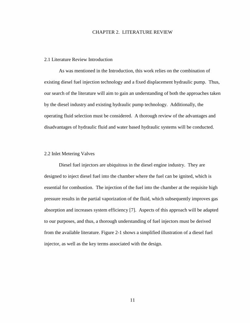
from the available literature. Figure 2-1 shows a simplified illustration of a diesel fuel
injector, as well as the key terms associated with the design.
12
Figure 2-1. Diesel Fuel Injector Diagram
The fuel injector is a solenoid operated valve that opens and closes as necessary to
allow fuel to flow through the orifice [8, 9]. Fuel injection pumps can also be used to
adjust the valve position [10]. Either way, the valve position controls both the quantity
(controlled by volume) and quality (controlled by pressure drop) of the fuel discharge
[11]. The fuel is driven by the pressure on the cylinder head, which can range from 2,000
to 20,000 psi [11]. As the needle is pushed downwards (based on the orientation
illustrated in Figure 2-), fuel is forced through the orifice [12]. The flow inside the
injector is impacted by dynamic factors like injection pressure and needle lift, as well as
the shape and finish of the orifice [13]. The flow out of the injector is partially vaporized
due to the pressure drop across the orifice and saturation pressure of the fuel. The
multiphase fluid is sprayed through the orifice and into the cylinder so that combustion
can occur during the mixing and evaporation process.
The control of the amount of fluid sprayed per charge is referred to as “metering”,
a term that will be applied to this work as well [2]. Fuel injection enables charge
stratification and detonation control [11]. This can reduce fuel consumption by
approximately 20% compared to chamber engines [15, 16]. They also decrease

13
emissions and improve engine startability, load acceptance (acceleration), and
combustion noise [11, 15]. It should be noted that while the fluid vaporization has
positive efficiency impacts in combustion, fluid vaporization can result in cavitation
damage in hydraulic systems [14]. This literature review will devote considerable study
to the impacts of cavitation on hydraulic systems later. For our application, many of the
previously listed efficiency advantages are negated. Instead, we focus on the fuel
injector’s ability to control the fluid quality. This control is what allows us to replace a
variable displacement pump with a fixed displacement pump.
2.3 Hydraulic Systems, A Brief History
Hydraulic systems have been used since 1795 when Bramah patented a hydraulic
press [18]. In 1802 hydraulic cranes were introduced [18]. Shortly after this, with the
advent of electricity, fluid power systems were neglected in favor of electrical power.
Blackburn provides an extensive comparison of fluid power and electricity, which has
been condensed into Table 2-1.
Table 2-1. Comparison of Fluid Power and Electric power [19]
Electric Power Fluid Power
Power
transmission over
distance
Relatively easy Relatively difficult
Controllability Easy at lower powers Easy at higher powers
Power density Limited by the fact that
ferromagnetic materials saturate
at low flux density
Very high torque to inertia ratio
Speed of Response Mechanically springy, relatively
slow response
Mechanically stiff, relatively
rapid response

14
Hydraulic systems maintained their space along the fringe of mechanical
technologies until World War II when their ease of control and high torque to weight
ratio made them ideal for warship gun turrets [20]. At this point, the United States
government began funding hydraulic control research. This influx of funding led to the
founding of the Servomechanisms Laboratory of the Massachusetts Institute of
Technology in 1939 [19]. Since that time, hydraulic systems have maintained their place
in both academia and industry.
2.3 A Comparison of Oil and Water Hydraulic Systems
Until the early 1900’s, all hydraulic systems in use relied on water. However, in
1906 Williams and Janney introduced the idea of replacing water with oil to avoid
corrosion and freezing, improve system lubrication, and decrease leakage [21]. This
trend of using oil continued until the 1970’s when the oil embargo caused a short term
increased interest in water hydraulics [22]. This interest petered out until the mid-
nineties when the engineering community began to take a serious look at reintroducing
water hydraulics into a variety of applications [21, 23].
Water based hydraulic systems have many advantages over oil. They are fire
resistant, low cost, non-toxic, and have lower disposal costs [22]. Water’s thermal
conductivity is four to five times greater than oil, so it requires significantly less cooling
capacity [21]. Water also contains much less air in solution than oil does, which
enhances the rigidity and safety of water hydraulic systems [23]. Water hydraulics have
a quicker response and higher efficiency than that of oil hydraulics [24]. Given the focus
that this work will devote to managing cavitation, perhaps the most significant

15
observation about water hydraulic systems is that given the same amount of cavitation in
a system, a system using hydraulic oil as the operating fluid will experience greater mass
loss than the system which uses water as the operating fluid [25]. This concept of mass
loss and erosion resistance will receive greater attention in subsequent sections of the
literature review.
Oil hydraulic systems have substantial environmental, flammability, and
regulatory concerns associated with them. For example, Europe has mandated that no oil
hydraulic systems be permitted in mines [26]. This means that water hydraulic systems
are the default technology in a variety of industries. These industries include nuclear
engineering, coal mining, steel foundries, desalination plants, fire-fighting, food and
beverage production, and plastic molding [21].
Obviously oil hydraulics would not be so ubiquitous in their use if water held all
of the advantages. Oil hydraulics are superior in respect to lubricity and rust resistance
[27]. The reduced lubrication of water means that the valve spools in those systems tend
to stick to the valve bodies, which causes more wear than would be experienced in a
traditional oil hydraulic system [28]. One way that this is frequently mitigated is by the
introduction of hydrostatic bearings into the spool valve [28, 29]. While this has been
shown to be an effective way of managing decreased lubrication, it requires additional
parts and increased machining. This is just one of many reasons why water hydraulic
systems can cost between 30 and 200% more than their oil hydraulic counterparts [22,
30]. Oil hydraulic systems are also known to be quieter than water hydraulics due to
their increased viscosity [31]. Further, lower viscosity of water results in increased
leakage when compared to oil based hydraulic systems [32].

16
Although oil based hydraulic systems fill the majority of fluid power applications,
water based systems have their place. Environmental concerns and increasing oil prices
should serve to increase the market share of water hydraulic systems. For our analysis,
we have elected to focus on a water hydraulic system given the readily available
thermodynamic properties and their small but significant presence in industry. It is more
difficult to find data on hydraulic oil systems since much of their material data is
proprietary.
The most significant differentiating factor between water and oil based hydraulic
systems for the purposes of our study is the discrepancy in saturation pressures. For
fluids with lower vaporization pressures, like water, gasoline, or diesel fuel, cavitation is
a crucial issue facing inlet metering valve implementation. Hydraulic oils have
vaporization pressures orders of magnitude greater than those fluids [33]. As a result, the
primary source of specific volume change for the hydraulic fluid is entrained air in the
system. Here the reader should recognize the significance of what has been said:
working fluid selection matters immensely in the inlet metering approach. Water based
systems will see part of the water vaporized as the result of the pressure drop, while oil
based systems will see air bubbles forming as the air comes out of solution. Both of these
topics will receive careful study in the subsequent literature review, although we
anticipate that cavitation will be of greatest concern for the system we have elected to
study.
17
2.4 Cavitation
Cavitation is the result of the rapid vaporization and subsequent condensation of a
liquid and can either be caused by an increase in temperature (e.g. boiling) or a decrease
in pressure. Nucleation sites, that is, the site where cavitation begins, can exist in two
different forms: dissolved gas or entrained gas. Dissolved gas does not affect the volume
or compressibility of the liquid at all; however, entrained gas is dispersed throughout the
liquid as bubbles and does impact the volume and fluid bulk modulus of the liquid [35].
Gaseous cavitation occurs when the fluid’s pressure drops below the saturation
pressure of the noncondensable gas (typically air) that is dissolved in the fluid [36]. It
occurs at a much slower rate than hydrodynamic cavitation, and can result in noise and
vibrations [37, 38]. This type of cavitation can be expected to appear with greater
frequency in hydraulic oil based systems, as hydraulic oil contains much more entrained
air than water does [23].
Hydrodynamic cavitation (also known as vaporous cavitation) is induced by a
rapid reduction in pressure from a higher pressure to the fluid’s saturation pressure. If the
local pressure remains depressed, the small cavity will continue to grow, and when the
pressure increases again, the cavity bubble will become unstable and collapse [35, 36].
This collapse is the cause of cavitation damage [37]. There are two means by which
cavitation damage can occur. The collapse can induce a shock wave in the liquid or an
asymmetric collapse can cause the bubble to lose its spherical shape and create a high
speed liquid jet which damages the solid surface [35]. This type of cavitation can be
expected to be more prevalent in water based hydraulic systems since water has a
saturation pressure several orders of magnitude smaller than hydraulic oil.
18
In 1965 the concept of erosion strength was first introduced in the literature.
Thiruvengadam defined erosion strength as the volume of material fractured on the
surface of the parent material by the work from an external force [39]. Since this
introduction, it has become the standard means by which to discuss a material’s ability to
resist cavitation. Erosion strength and erosion resistance are two terms used to describe a
numeric property that provides designers with a way to choose the appropriate material to
withstand cavitating conditions.
Substantial effort has been exerted to uncover relationships between well-known
material properties like hardness and the lesser understood erosion resistance. Hattori et
al found that the erosion resistance of carbon steel, excluding stainless steel, increases
proportionally (to the power of 2.4) with the Vickers hardness [40], and later published a
correlation for the erosion resistance of stainless steel that accounts for the work
hardening that occurs during cavitation [41]. Heymann observed that erosion resistance
is strongly correlated (to the power of 2.5) with material hardness for nine other materials
[42]. Varga conducted similar studies and developed relationships between material
properties and the normalized erosion resistance for cast bronzes, wrought bronzes,
nickel alloys, aluminum alloys, and titanium alloys [43].
Other numerically expressed properties have been identified to help us talk about
cavitation. For example, the cavitation index is a metric that has been developed in order
to predict the formation of cavitation, and it has been directly correlated to performance
breakdown, noise and erosion [44]. When considering insertion of cavitation resistant
materials as a means to protect the pump from cavitation damage, investigation of the
material’s cavitation index will be a useful metric.
19
2.5 Machine Design Considerations
Cavitation can occur in both spool valves and pumps. Large pressure differences
across valve chambers and high frequency motion of valve-controlled actuators can
induce cavitation in spool valves [45]. In pumps, cavitation occurs when the pressure in
the piston cylinder drops rapidly at the beginning and end of the pump’s suction stroke
due to the small opening area of the cylinder port [38]. Because of the aforementioned
undesirable effects, one of the primary objectives of hydraulic system design is often to
avoid cavitation in the pump [41]. In addition to the noise, vibrations, and damage,
serious reduction of the pump’s filling performance can result from cavitation [46]. This
is another reason to actively design against gaseous cavitation.
The literature is full of examples of engineers working to avoid cavitation. Wang
redesigned the valve plate in the axial piston pump to reduce the development of
cavitation in the piston barrels [51]. Suzuki and Urata designed a valve with two serial
throttles to mitigate cavitation in a pressure reducing valve for a water hydraulic system
[47]. Their work was derivative of the work of Liu who also utilized multiple throttles to
cause a stepwise pressure drop rather than a rapid decrease in pressure [48]. Manring
explored different flow passage geometries to cause a gradual pressure reduction rather
than a steep pressure drop [49].
The breadth of literature in regards to designing pumps and valves to avoid
cavitation indicates the emphasis that has been placed on cavitation avoidance in the
scientific community. In addition to geometry design, another approach frequently taken
is to simply install inserts in the pumps that are highly resistant to cavitation damage [52].
It should be noted that, particularly for water hydraulic systems, stainless steel and

20
ceramic materials have been found to be highly cavitation-resistant [29, 30, 34]. Metallic
composite interfaces have been observed to be the best option in axial piston water
pumps and motors [18].
2.6 Entrained Air
Entrained air is an issue that applies specifically to hydraulic oil based systems.
Water hydraulic systems are able to use the inlet metering technique to induce fluid
vaporization. Therefore, this section is less likely to apply to them. The saturation
pressure of the air in hydraulic oil systems is much lower than that of the oil, thus the
behavior of entrained air becomes highly significant.
Air becomes entrained in the hydraulic fluid when a volume of air is trapped in
the fluid and subsequently breaks into a set of bubbles [53]. These bubbles are then
transported along by the fluid flow and can either continue as entrained air or, if
pressurized, shift to dissolved air, which has no impact on the fluid volume [54]. The
process by which air becomes entrained is also known as aeration [55].
Entrained air results in a significant reduction of the effective fluid bulk modulus,
and subsequently slows the system responsiveness [56]. It should be noted here that
although entrained air has this negative impact on the system, dissolved air does not
impact fluid bulk modulus [57]. Entrained air can also result in pressure pulsations, air
binding, increased noise, poor pump suction performance [58], filter blocking [59], and
increased throttling losses [60]. Whether the hydraulic system experiences cavitation or
aeration, similar damage can result from either [55]. However, for all these negative
impacts, substantial effort in the literature has been devoted to intentionally adding

21
entrained air to the system. When there is less than 5% but more than 0% (more
specifically, between 0.3% and 1.0%) of air entrained in the system, it has been showed
to cushion the implosive effects of cavitation and actually improve pump performance
[52, 58, 61].
After aeration has occurred, the best way to change the volumetric ratio of liquid
to air in the system is done by adjusting the inlet pressure [58]. Temperature adjustment
is the main means of controlling the aeration within the fluid [59]. Further consideration
of both of these approaches would be necessary if introducing inlet metering valves to a
hydraulic system which uses hydraulic oil.
The inlet metering valve relies on fluid vaporization to change the volume of the
working fluid in order to maintain control of the pump output flow. Due to the high
vaporization pressure of hydraulic oil, vaporizing the fluid in order to adjust its specific
volume is not an option. Instead, hydraulic fluid specific volume adjustments would be
made by dissolved and entrained air modulation. The inlet metering valve in a water
hydraulic system, on the other hand, is able to rely on fluid vaporization as discussed
previously.
2.7 Fluid Modeling Justification
In addition to the similarities the inlet metering valve in our hydraulic system
design has to the diesel fuel injector, our inlet metering design shows similarities to
aspects of a refrigeration system. A typical vapor-compression refrigeration process
consists of four major components: a condenser, a compressor, an evaporator, and an
expansion valve [62]. This expansion valve is the location where the refrigeration fluid
makes the transition from saturated liquid to two-phase liquid-vapor mixture. Similarly,

22
our inlet metering valve marks the location in the system where the working fluid, in our
case, water, transitions from saturated liquid to liquid-vapor mix.
A throttling process always occurs when a flowing fluid experiences an abrupt
pressure decrease when passing through a restricted opening [63]. Thus, throttling occurs
in both the expansion valve associated with refrigeration cycles and in our inlet metering
valve. Since our inlet metering valve is novel and no literature exists to suggest the best
approach to modeling the phase change that occurs at the valve restriction, the best
approximation to be found is to study the literature that exists on refrigeration cycles.
A survey of the literature finds that a particular area of focus in refrigeration cycle
studies has been on the increase of efficiency. This is unsurprising; the search for greater
efficiency is prevalent in virtually every developed technology. The question we are
most interested in, though, is how does the scientific community theoretically model the
refrigeration systems that they are studying?
Evidence of usage of both the first law of thermodynamics and the second law of
the thermodynamics can be found. In his review of the literature on vapor compression
refrigeration systems, Ahamed et al asserts that the first law analysis is the most common
approach to the analysis of thermal systems, and that the energy performance of heating,
ventilation and airconditioning (HVAC) systems are most frequently evaluated with the
first law [64]. Examples of this are plentiful. Hasan et al uses a first law analysis to
study the amount of energy converted to a useful energy output in a refrigeration cycle
that relies on a solar heat source [65]. Khaliq et al use a first law analysis to study the
efficiency of a refrigeration cycle that takes advantage of an ejector to increase efficiency
[66].

23
The exergy analysis made possible by use of the second law of thermodynamics is
also incredibly prevelant in the refrigeration literature [67- 69]. The second law appears
to be most effective at revealing system irreversibilities [64, 70]. After the
irreversibilities are identified, they can be reduced using Bejan’s exergy minimization
principle [71]. The minimization of exergy generation will improve system performance.
Rakopoulos et al recommends coupling a first law analysis with a second law analysis for
system optimization, in order to identify the maximum system performance point [70].
For our preliminary modeling, then, we will perform a first law based analysis to
study the efficiency of our inlet metering system. This efficiency analysis will be
presented in Chapter 4. The exergy analysis appears to be most useful when considering
a system dealing with multiple working fluids (e.g. water and air as in an HVAC system).
In this initial work on an inlet metering system, we will not perform an exergy analysis;
however, it may be a topic of interest in the future.
In 1950, Joseph Keenan published “An investigation of ejector design by analysis
and experiment.” This work appears to be fundamental to much of the refrigeration cycle
analysis done today. In his study, he introduces the one-dimensional constant pressure
flow model. This model assumes that the pressures of both the liquid and vapor flowing
in the system are perfectly mixed and exist at identical pressures [72]. Notably, he
acknowledges the risk of choking in his system, but elects to neglect this issue even
though it had been observed in experiments that he had knowledge of. Further
development of this model was conducted by Huang, who addresses choking in the
nozzle [73].

24
Much more recently, in 2007, Guo-liang Ding published a review of the recent
approaches to simulations of refrigeration systems. Homogeneous flow, an assumption
that we will be applying to our work, is still a commonly accepted model that can be used
to simplify calculations associated with multiphase flow [74]. This assumption implies
that the system changes phase under thermodynamic equilibrium, there is no slip between
the liquid and vapor phases, and there is complete mixing between the liquid and vapor
phase. This will lead to a lower entropy production value than we would otherwise
generate; the irreversible thermodynamic transitions that occur during two phase flows
are a source of entropy production [75]. While this omission of one of the sources of
entropy in our system will be present in our model, this assumption is prevalent in much
of contemporary refrigeration literature and thus we will apply it here as well. Ding also
recommends using look up tables for thermodynamic properties of the refrigerant [74].
We will also rely heavily on published and established thermodynamic property tables for
water in our system evaluation.
An example of the application of the one-dimensional pressure flow model can be
seen in the work by Wang et al. In this work, the authors use thermodynamic look up
tables, the first law of thermodynamics, and principles from the conservation of mass and
conservation of energy to analyze their system [76]. We will also apply all of these tools
to our study of the inlet metering system. Most notably, in all of the refrigeration
literature that was read in preparation for this dissertation, no theoretical handlings of the
effects of air mixing with the refrigerants selected as working fluids were observed [65,
69, 72]. Instead the authors performed their analysis under the assumption that their
working fluid was pure and unchanged by entrained or dissolved air. For our analysis,

25
too, then we will proceed as though our working fluid (water) is pure and unaffected by
entrained or dissolved air. Having made this assumption, we will then be able to apply
the principle of fluid quality, that is, the mass fraction of the vapor present in a given
volume of working fluid relative to the total mass of that volume of working fluid [62].
This will prove to be a key parameter in Chapter 3’s analysis.
2.8 Literature Conclusions
The literature search has revealed that cavitation effects in hydraulic systems have
been studied quite thoroughly, as have the cavitating abilities of inlet metering valves in
fuel injection systems. However, no results have been found to suggest that inlet
metering technology has been applied to hydraulic systems, whether oil or water based.
This suggests that our work is novel.

26
CHAPTER 3. ANALYSIS
3.1 Analysis Introduction
The purpose of this analysis is to develop a theoretical model of an inlet metering
pump. Here we will develop a computationally inexpensive method to determine the
percent of fluid that is vaporized during the operation of this pump, illustrate the control
related impacts of vaporized fluid on the operation of the pump, and derive a coupled set
of differential equations that describe the dynamics of the valve and pressure output of
the pump. In Section 3.14, we will nondimensionalize the coupled set of differential
equations. At the end of this chapter, the theoretical model for a variable displacement
pump will be introduced. This model will be used for comparison’s sake in Chapter 6.
3.2 Transient Pressure Analysis
The pressure rise rate equation is given as Eq. (3.1) [20]. As we seek to control
the output pressure of the pump, a cursory glance at Eq. (3.1) reveals that we must also
know the pump output flow Q2, the fluid volume at the pump outlet (note that this is not
to be confused with the fluid specific volume), V2, the leakage associated with the pump,
K, and the fluid bulk modulus .
2 2 2
2
sysP Q KP QV
(3.1)
We will assume a constant leakage value. The literature suggests that 10% is
reasonable for a water hydraulic system, so a value of max
max10
QK
P will be used [47].

27
The fluid specific volume at the pump outlet and the fluid bulk modulus will also be
treated as constant. There are a significant number of published thermodynamic property
tables that provide specific volume of water at a given pressure and temperature. These
will be used throughout the analysis. The subsequent section will deal with determining
the pump output flow, Q2.
3.3 Pump Discharge Flow
As mentioned in the introduction, variation of the inlet metering valve cross-
sectional area results in a change in the pump discharge flow rate. This section will
explore how the pump output flow is affected by the valve area. Figure 3.1 shows the
piston pump, crankshaft and check valves associated with the pump design, as well as the
nomenclature that will be used.
Figure 3-1. Piston pump
r
28
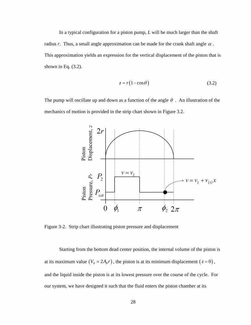
In a typical configuration for a piston pump, L will be much larger than the shaft
radius r. Thus, a small angle approximation can be made for the crank shaft angle .
This approximation yields an expression for the vertical displacement of the piston that is
shown in Eq. (3.2).
1 cosz r (3.2)
The pump will oscillate up and down as a function of the angle . An illustration of the
mechanics of motion is provided in the strip chart shown in Figure 3.2.
Figure 3-2. Strip chart illustrating piston pressure and displacement
Starting from the bottom dead center position, the internal volume of the piston is
at its maximum value 2P PV A r , the piston is at its minimum displacement 0z ,
and the liquid inside the piston is at its lowest pressure over the course of the cycle. For
our system, we have designed it such that the fluid enters the piston chamber at its

29
saturation pressure. This fluid will be a mixture of liquid and vapor, the specific
percentages of which are dictated by the inlet metering valve cross-sectional area.
Once the piston begins to move upwards, (the angle increases from 0 to a
specific value 1 ), the pressure inside the piston chamber increases. As the pressure
increases to a value of 2P , the vaporized fluid condenses until all of the fluid in the
piston is liquid. Once the fluid is fully condensed, the check valve downstream from the
pump (shown in Fig. 3.1) opens. This occurs at piston position 1 . From piston position
1 to position , the piston forces the fluid out of the chamber and through the check
valve downstream from the pump. Once the piston reaches its maximum height
2z r , all of the fluid exiting the piston chamber for that given stroke will have been
forced out of the piston. A small volume of fluid will remain in the chamber. As the
piston moves from position to position 2 the remaining fluid will vaporize until it
reaches a pressure level equal to that of the fluid which is waiting upstream from the first
check valve. At position 2 the first check valve will open; and as the piston moves
downward, the space that it vacates will be filled by the partially vaporized fluid coming
from the inlet metering valve. This will continue until the piston chamber is again
completely filled with a vapor/liquid mix at position 0 . Then the piston will move
upwards, and the cycle continues.
The contracted valve area induces partial fluid vaporization for the fluid entering
the pump. Our means of talking about fluid vaporization throughout this paper will rely
on a discussion of fluid quality, which refers to the percentage of vaporized fluid in the
working fluid on a per mass basis.
30
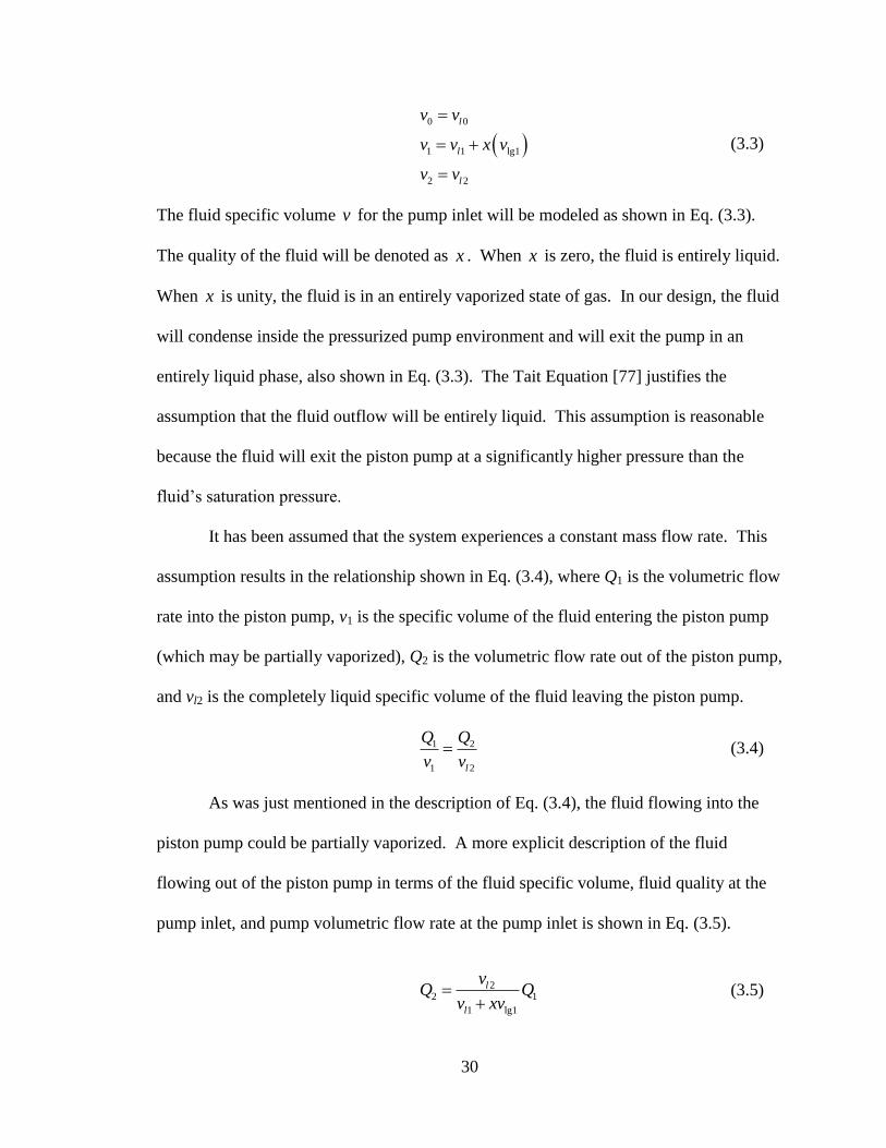
0 0
1 1 lg1
2 2
l
l
l
v v
v v x v
v v
(3.3)
The fluid specific volume v for the pump inlet will be modeled as shown in Eq. (3.3).
The quality of the fluid will be denoted as x . When x is zero, the fluid is entirely liquid.
When x is unity, the fluid is in an entirely vaporized state of gas. In our design, the fluid
will condense inside the pressurized pump environment and will exit the pump in an
entirely liquid phase, also shown in Eq. (3.3). The Tait Equation [77] justifies the
assumption that the fluid outflow will be entirely liquid. This assumption is reasonable
because the fluid will exit the piston pump at a significantly higher pressure than the
fluid’s saturation pressure.
It has been assumed that the system experiences a constant mass flow rate. This
assumption results in the relationship shown in Eq. (3.4), where Q1 is the volumetric flow
rate into the piston pump, v1 is the specific volume of the fluid entering the piston pump
(which may be partially vaporized), Q2 is the volumetric flow rate out of the piston pump,
and vl2 is the completely liquid specific volume of the fluid leaving the piston pump.
1 2
1 2l
Q Q
v v (3.4)
As was just mentioned in the description of Eq. (3.4), the fluid flowing into the
piston pump could be partially vaporized. A more explicit description of the fluid
flowing out of the piston pump in terms of the fluid specific volume, fluid quality at the
pump inlet, and pump volumetric flow rate at the pump inlet is shown in Eq. (3.5).
22 1
1 lg1
l
l
vQ Q
v xv
(3.5)

31
Equation (3.5) clearly illustrates that the pump discharge flow is a function of the inlet
fluid quality. For example, consider the case where the inlet fluid is fully condensed
0x . If we recognize that the outlet flow specific volume 2lv is nearly identical to the
inlet flow specific volume 1lv (the outlet flow specific volume will be slightly, though
insignificantly, higher than the inlet flow specific volume due to the higher outlet
pressure), we can observe that the discharge flow rate is simply equal to the pump inlet
flow rate. (The assumption that 1 2lo l lv v v will be applied throughout this analysis.)
If, however, we consider a fully vaporized fluid 1x and recognize that lg1 1lv v ,
we can see that the discharge flow rate of the pump becomes very small. From this, we
find that we have created a variable-displacement pump utilizing a fixed displacement
pump, and an inlet metering valve that allows us to exert control over the fluid quality at
the inlet.
The pump experiences a different flow rate for each of the phases described by
Fig. 3-2. The following analysis will explore the pump behavior for each of these
conditions. Then an analysis of the relationship between the valve’s cross sectional area
and the fluid quality will be completed.
3.4 Pump Flow Phase I: 0 < θ < ϕ1
When the pump begins its upstroke, from 10 , the fluid is condensing.
The maximum volume of the pump occurs at 0 and the mass of the fluid that fits
inside the piston volume can be given as Eq. (3.6).
max
lgl
Vm
v v x
(3.6)

32
At the bottom of the piston stroke, the fluid is a mixture of vapor and liquid and
will vary as a function of the fluid quality. Once the crankshaft reaches the position 1
the fluid is fully condensed lv v . At this point, we can calculate the exact position of
the crankshaft as a function of our piston internal maximum volume and fluid quality.
This derivation is shown in Eq. (3.7).
max 1max
lg
2 1 cosP
l l
V A rV
v v x v
(3.7)
The nondimensional groups shown in Eq. (3.8) are used to nondimensionalize Eq. (3.7).
The specific volume ratio, v , and pump volume ratio, V , will both be key parameters
considered throughout the analysis.
lg
max
ˆˆ and p
l
v A rv V
v V (3.8)
1
ˆcos 1
ˆ ˆ1
vx
V vx
(3.9)
A nondimensional expression for the crankshaft position at the point where our fluid is
fully liquid, 1 , is given as Eq. (3.9). This is derived by applying the specific volume
ratio and pump volume ratio to Eq. (3.7). From this expression, it is evident that the
rotation required to condense our fluid is a function of the thermodynamic properties of
the fluid ( lv and lgv ) , the dimensions of the piston itself ( pA , r, and maxV ), and the
quality of the fluid entering the piston (x).
33
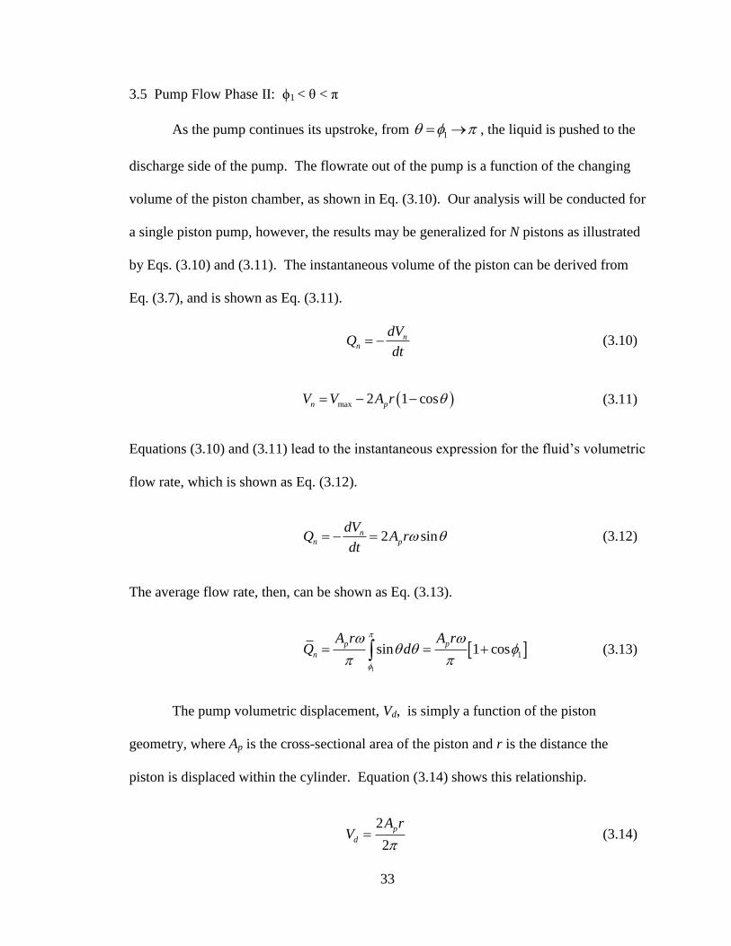
3.5 Pump Flow Phase II: ϕ1 < θ < π
As the pump continues its upstroke, from 1 , the liquid is pushed to the
discharge side of the pump. The flowrate out of the pump is a function of the changing
volume of the piston chamber, as shown in Eq. (3.10). Our analysis will be conducted for
a single piston pump, however, the results may be generalized for N pistons as illustrated
by Eqs. (3.10) and (3.11). The instantaneous volume of the piston can be derived from
Eq. (3.7), and is shown as Eq. (3.11).
nn
dVQ
dt (3.10)
max 2 1 cosn pV V A r (3.11)
Equations (3.10) and (3.11) lead to the instantaneous expression for the fluid’s volumetric
flow rate, which is shown as Eq. (3.12).
2 sinnn p
dVQ A r
dt (3.12)
The average flow rate, then, can be shown as Eq. (3.13).
1
1sin 1 cosp p
n
A r A rQ d
(3.13)
The pump volumetric displacement, Vd, is simply a function of the piston
geometry, where Ap is the cross-sectional area of the piston and r is the distance the
piston is displaced within the cylinder. Equation (3.14) shows this relationship.
2
2
p
d
A rV
(3.14)

34
Equation (3.15) shows the average result associated with Eq (3.13), utilizing the
groups provided earlier in Eq. (3.8) and the expression for volumetric displacement
shown in Eq. (3.14). From this, we can observe that the volumetric flow rate remains a
function of the thermodynamic properties of the fluid, the dimensions of the piston itself,
and the quality of the fluid entering the piston. It is also affected by the speed of the
crank shaft ( ), which was not the case for the condensation process.
2
ˆ1
ˆ ˆ2 1d
vxQ V
V vx
(3.15)
3.6 Pump Flow Phase III: π < θ < ϕ2
As the pump begins its downstroke (from 2 ), the small amount of fluid
that remains in the piston chamber (the fluid that was not expelled at the maximum height
of the piston upstroke) is vaporized back to the quality associated with the fluid waiting
upstream of the check valve. The exact location of 2 can be found in a method similar
to the derivation provided in the Pump Flow Phase I calculation. It again relies on the
nondimensional groups provided in Eq. (3.8). The result is shown in Eq. (3.16).
2
ˆ ˆ2 1cos 1
ˆ
V vx
V
(3.16)
Equation (3.16) shows that 2 is a function of the thermodynamic properties of the fluid,
the dimensions of the piston itself, and the quality of the fluid entering the piston. These
are the same parameters associated with the identification of 1 in Eq. (3.9)

35
3.7 Pump Flow Phase IV: ϕ2 < θ < 2π
As the pump continues its downstroke, the upstream check valve opens and the
partially vaporized fluid mixture is drawn into the pump. The volumetric flow rate of this
fluid is still dictated by the relation given as Eq. (3.12) and can be expressed as shown in
Eq. (3.17). It is a function of the thermodynamic properties of the fluid, the dimensions
of the piston itself, the quality of the fluid entering the piston, and the speed of the crank
shaft, which is the same list of parameters that shapes the average flow rate exiting the
pump as described in Eq. (3.15).
1
ˆ ˆ1 21
ˆ2d
V vxQ V
V
(3.17)
3.8 Pump Flow Summary
Table 3-1 shows the volumetric flow rate entering or exiting the pump at each
point along the cycle illustrated by Figs. 3-1 and 3-2. The locations of 1 and 2 are a
function of the fluid quality leaving the inlet metering valve, and are given by Eqs. (3.9)
and (3.16) respectively. From Table 3-1 it can be observed that a derivation of the fluid
quality as a function of our valve geometry would be extremely useful. This will be done
in Section 3.9.

36
Table 3-1. Summary of pump flow behavior at throughout the cycle
Pump Flow Phase Crankshaft
Location Volumetric Flow Rate
Pump Flow Phase I 10 0Q
Pump Flow Phase II 1
2
ˆ1
ˆ ˆ2 1d
vxQ V
V vx
Pump Flow Phase III 2 0Q
Pump Flow Phase IV 2 2
1
ˆ ˆ1 21
ˆ2d
V vxQ V
V
3.9 Inlet Metering Valve
Figure 3.3 shows the inlet metering valve, where Ao is the cross-sectional area at
the valve inlet, and A1 is the cross-sectional area at the valve outlet. For simplicity of
calculations, it will be assumed that the valve openings are identical squares. The
dimensions of the fully open orifice are max maxy y . Ao is fixed, and A1 varies linearly
with the valve displacement y. This is written explicitly in Eq. (3.18).
2
max
1 max
oA y
A yy
(3.18)
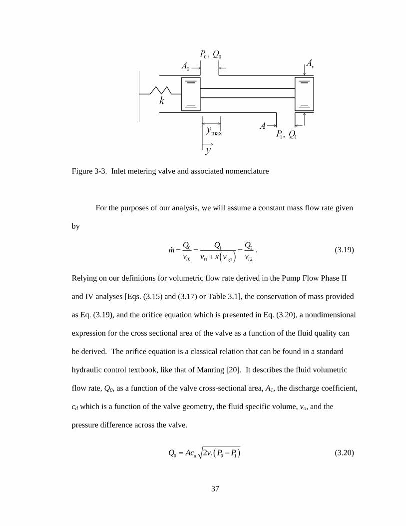
37
Figure 3-3. Inlet metering valve and associated nomenclature
For the purposes of our analysis, we will assume a constant mass flow rate given
by
0 1 2
0 21 lg1l ll
Q Q Qm
v vv x v
. (3.19)
Relying on our definitions for volumetric flow rate derived in the Pump Flow Phase II
and IV analyses [Eqs. (3.15) and (3.17) or Table 3.1], the conservation of mass provided
as Eq. (3.19), and the orifice equation which is presented in Eq. (3.20), a nondimensional
expression for the cross sectional area of the valve as a function of the fluid quality can
be derived. The orifice equation is a classical relation that can be found in a standard
hydraulic control textbook, like that of Manring [20]. It describes the fluid volumetric
flow rate, Q0, as a function of the valve cross-sectional area, A1, the discharge coefficient,
cd which is a function of the valve geometry, the fluid specific volume, vo, and the
pressure difference across the valve.
0 0 12d lQ Ac v P P (3.20)

38
Substitution of Eqs. (3.17) and (3.20) into Eq. (3.19) yields Eq. (3.21).
0 1
ˆ ˆ1 212 1
ˆˆ1 2d l d
V vxAc v P P V
vx V
(3.21)
We then define the valve dimensions according to Eq. (3.22). This convenient definition
will enable us to solve Eq. (3.21), which results in Eq. (3.23).
0 1
ˆ
2
d
d l
VA A
c v P P
(3.22)
ˆ ˆ ˆ2 1 2ˆ
ˆ ˆ2 1
V V vxA
V vx
(3.23)
Equation (3.23) can be simplified due to the relative magnitudes of the non-
dimensional groups from Eq. (3.8). This simplification is shown as Eq. (3.24).
ˆˆ 1ˆ2
vxA
V (3.24)
Rearranging Eq. (3.24) provides an expression for the fluid quality in terms of valve
outlet area. This result is shown as Eq. (3.25).
ˆ ˆ1 2
ˆ
A Vx
v
(3.25)
The volumetric flow rate can be nondimensionalized using the pump volumetric
displacement and shaft speed, as shown in Eq. (3.26)
2 2 2ˆ ˆp
d
A rQ V Q Q
(3.26)

39
Recall the definition for the fluid outlet volumetric flow rate given by Eq. (3.15).
Substitution of the relation for fluid quality from Eq. (3.25) into Eq. (3.15) and the
nondimensional expression for volumetric flow rate in Eq. (3.26) yields a simplified
approximation for the volumetric flow rate. Observe that Eq. (3.27) matches the result
for the nondimensional valve cross sectional area, A , which was presented in Eq. (3.23).
2
ˆˆ 1ˆ ˆ2 1
vxQ
V vx
(3.27)
Normalizing the volumetric flow rate about the condition where x=0 leads to a simplified
expression for the nondimensional volumetric flow rate.
2
ˆˆ 1ˆ2
vxQ
V (3.28)
Recall the definition for the nondimensional valve cross-sectional area given in Eq. (3.24)
. A comparison between Eqs. (3.24) and (3.28) (or Eqs. (3.23) and (3.27)) reveals a
direct relationship between the volumetric flow rate and valve cross-sectional area.
2ˆ ˆQ A (3.29)
Equation (3.29) shows that the discharge flow of the pump is directly proportional to the
cross-sectional area of the inlet metering valve which provides a very nice relationship
from a control point of view.
In order to apply the pressure rise rate equation from Eq. (3.1), a second
expression for the flow exiting the pump must be developed. The pressure rise rate
equation will rely on the previously presented orifice equation (Eq. (3.20)). Recall the
conservation of mass (Eq. (3.19)). By definition, then, 0 2Q Q if we assume the specific

40
volume of all purely liquid quantities of the working fluid are constant (0 1 2l l lv v v ).
This result is provided in Eq. (3.30)
2 1 0 0 12d lQ Ac v P P (3.30)
Recall Eq. (3.18) which shows the relationship between valve areas and valve
displacement. Thus, the volumetric flow rate can be rewritten in terms of valve
displacement y. This result is shown in Eq. (3.31).
2 max 0 0 12d lQ y c v P P y (3.31)
Revisiting the pressure rise rate equation [Eq. (3.1)] and substituting the leakage
coefficient and pump outlet expression into it yields the pressure rise rate equation in
terms of valve displacement y. This is given as Eq. (3.32).
2 max 0 0 1 2
2
2d l sysP y c v P P y KP QV
(3.32)
Equation (3.32) will then be normalized about the steady state volumetric flow rate. This
will be done by solving the steady state system. The result is given as Eq. (3.33)
, max 0 0 12sys ss d l ss ssQ y c v P P y KP (3.33)
Substitution of Eq. (3.33) into Eq. (3.32) yields a normalized expression about the steady
system scenario where yss and Pss are the steady-state valve displacement and steady-state
pressure respectively. This result is given as Eq. (3.34).
2 max 0 0 1 2
2
2d l ss ssP y c v P P y y K P PV
(3.34)

41
In the following section, a second expression for valve displacement will be derived.
This is necessary for control law development.
3.10 Valve Flow Force Considerations
A free body diagram of the inlet metering valve is shown as Fig. 3-4. The valve
experiences stabilizing forces from the spring and downstream pressure (the resulting
force from P2 is called Fy), as well as a destabilizing force from the internal flow forces
associated with the fluid slug inside the valve.
Figure 3-4. Inlet metering valve free body diagram
The dynamic equation for the valve, based on Fig. 3-4, is given in Eq. (3.35),
where mv is the mass of the spool valve, Fo is the initialized spring force, k is the spring
constant, c is the drag coefficient associated with the valve displacement, Fy is the force
on the valve that results from application of pressure, P2, on the cross sectional area of
the valve spool, Av, and Fi is the summation of all internal horizontal flow forces within
the valve.
ˆv o y im y F ky F F cy (3.35)

42
3.11 Flow Force Analysis
In order to find the internal flow force, Fi, the Reynolds Transport Theorem will
be used. A derivation of the Reynolds Transport Theorem can be found in a typical
fluids textbook [78]. The Reynolds Transport Theorem is given in Eq. (3.36). It may be
helpful to observe that vector quantities are denoted by boldface type.
ˆCV CS
dV dAt
F u u u n (3.36)
Figure 3-5. Inlet metering valve flow at the outlet
Expanding the Reynolds Transport Theorem for the geometry in Fig. 3-5 yields
Eq. (3.37).
0 1 0 1
0 0 1 1 0 0 0 0 1 1 1 1ˆ ˆ
V V A A
dV dV dA dAt t
F u u u u n u u n (3.37)
The vector expressions associated with the Reynolds Transport Theorem and based on
the geometry in Fig. 3-5 are given in Eq. (3.38). The fluid velocity is described by the
vector quantity u and the normal vector component is written as n.

43
0 1 10 1
0 1 1
0 1
0 cos sin
ˆ ˆ1 0 cos sin
Q Q Q
A A A
u i j u i j
n i j n i j
(3.38)
Observe that the force described by the Reynolds Transport Theorem is simply a vector
as illustrated in Eq. (3.39).
x yF F F i j (3.39)
The force can be broken up into components as shown in Eq. (3.39). Substituting the
vector quantities from Eq. (3.38) into Eq. (3.37) and then separating the result into
components yields Eq. (3.40). The application of the Reynolds Transport Theorem is
covered extensively by Manring [20].
2
0
1
2
0
1 1
cos
sin
i
o o
j
QL dQF
v dt Av
QF
Av
(3.40)
The orifice equation was given earlier in Eq. (3.31). The transient volumetric
flow force can then be written as Eq. (3.41).
10 12d o
dAdQc v P P
dt dt (3.41)
Applying Eqs. (3.18), (3.40), and (3.41) yields an expression for the internal horizontal
flow force in terms of valve displacement. This equation elicits a description of the force
that results from the changing momentum of the fluid slug within the valve.

44
2
max 0 1 0 1 max2 2 c y cosi d o d
o
L dyF y c v P P P P y
v dt (3.42)
For simplicity, the leading coefficients in Eq. (3.42) will be defined by the
groupings in Eq. (3.43)
1 0 1 max
2
2 0 1 max
2
2 cos
d o
o
d
Lc v P P y
v
P P c y
, (3.43)
which then produces the following expression for the horizontal force associated with the
fluid slug momentum
1 2i
dyF y
dt . (3.44)
Thus the expression for the changing fluid momentum can be rewritten as Eq. (3.44)
utilizing the groups defined in Eq. (3.43).
The angle in Eqs. (3.42) and (3.43) (and shown in Figure 3.5) is the angle at
which the fluid exits the valve outlet. This is called the jet angle, which was classically
derived by Von Mises in 1917 [79]. The jet angle solution from Von Mises is given in
Eq. (3.45) [80], where cr is the radial clearance within the valve and y is the valve
displacement.

45
1 sin ln tan cos2 2
21 cos ln tan sin2 2
r
y
c
(3.45)
In order to approximate Eq. (3.45) for the purposes of our analysis, a constant jet
angle was assumed. Merritt states that this is an entirely realistic approximation,
particularly for a valve that operates typically between 75% and 100% of the maximum
valve opening [54]. Merrit suggests that 69o is an accurate approximation; however,
Yang et al makes a compelling argument that specifically for water hydraulics, 64o is
better [24, 54]. In his work, "Water hydraulics-A novel design of spool-type valves for
enhanced dynamic performance", he engages in an extensive CFD analysis of a variety of
spool valve geometries and for multiple fluid viscosities (simulating both water and
mineral oil) and validates Merritt’s assertion for mineral oil. However, he notes that the
efflux angle is impacted by the reduced fluid viscosity of water, and that a slightly
smaller jet angle is more representative [24]. His CFD results clearly illustrate this point,
and thus, 64o will be used throughout the analysis.
3.12 Full Dynamic Valve Equation
The valve dynamics can be fully depicted by applying Eq. (3.42) to Eq. (3.35).
The full valve equation is given as Eq. (3.46).
1 2 2v o valvem y c y k y F P A (3.46)

46
The spring initialized force, Fo, can be determined by solving Eq. (3.46) for a steady
system. The spring force is shown as Eq. (3.47).
2o valve ss ssF A P k y (3.47)
Substitution of Eq. (3.47) into Eq. (3.46) yields a normalized expression about the steady
system scenario where yss and Pss are the steady-state valve displacement and steady-state
pressure respectively. This is given as Eq. (3.48).
1 2v ss valve ssm y c y k y y A P P (3.48)
3.13 Summary of Dimensional Equations
Eq. (3.49) shows the coupled set of differential equations that describe the motion
of the inlet metering spool valve. The derivation of the pressure rise rate equation
reached its conclusion in Eq. (3.34), and the derivation of outlet pressure as a function of
the valve was concluded in Eq. (3.48).
max 0 0 1
2
1 2
1. 2
2.
d l ss ss
vss ss
valve valve valve
P y c v P P y y K P PV
m c ky y y y P P
A A A
(3.49)
3.14 Nondimensionalization
Several methods exist to identify the most significant terms in a dynamic
equation. Numerical regression can be used [81]. Development of nondimensional
groupings for applied sensitivity analysis is another option [82, 83]. This second

47
approach seems to be a more expedient process which is easily adjusted to varying
system parameters. As such, this will be the method employed in this analysis.
Taking a nondimensional approach to Eq. (3.49) enables simplification of our
system of equations. By identifying nondimensional groupings in our key equations, we
will be able to compare the relative magnitudes of the nondimensional groups and
determine which terms contribute most significantly to the system dynamic behavior.
After we identify the insignificant terms, we can eliminate the higher order differential
terms in our expression. A lower order system will behave with less overshoot and
oscillation; it is helpful to determine if our system can be reduced. Eqs. (3.50) and (3.51)
show the important nondimensional term definitions that will be used in our analysis.
2ˆ ˆˆss ss
Vy y y P P P t t
K
(3.50)
max 0 0 1 2
1 2
1
2
2ˆ ˆ
ˆ ˆ
ss d l ss
ss valve ss
ss v ss
valve ss valve ss
y y c v P P k yK K
KP A P
c y m yc m
A P A P
(3.51)
The nondimensional groups given in Eqs. (3.50) and (3.51) can be applied to Eq. (3.49)
in order to yield the nondimensional description of the system given as Eq. (3.52).
1 1
2 2
ˆ ˆ ˆ ˆˆ1. P 1
ˆ ˆ ˆˆ ˆ ˆˆ ˆ2. 1
P K y K
my cy K y P K
(3.52)
Observe that for steady-state operations, the nondimensional pressure, P , must be
equivalent to the nondimensional valve displacement, y . In order for this to be true,
48
design guidelines should be established such that the nondimensional leakage coefficient
1K is unity. The design guidelines requisite for this scenario will be discussed further in
Chapter 5, but for now it is sufficient to assert that the nondimensional leakage
coefficient can be designed to achieve this aim. The resulting set of nondimensional
equations, then can be shown in Eq.(3.53).
2 2
ˆ ˆ ˆ1. P
ˆ ˆ ˆˆ ˆ ˆˆ ˆ2. 1
P y
my cy K y P K
(3.53)
The nondimensional set of equations in Eq. (3.53) comprises the most important
contribution of this analysis. From this result, we will be able to investigate the
efficiency of the system (Chapter 4), study the stability of the system (Chapter 5),
develop design criteria and rules of thumb for engineers looking to apply this technology
(Chapter 5), and model the dynamic behavior of our system (Chapter 6). In Chapter 6 we
will solve Eq. (3.53) for a variety of design scenarios. This will show the behavior of the
inlet metering system and illustrate its ability to maintain a downstream steady-state
pressure.
3.15 Variable Displacement Pump Model
Because we are interested in comparing the dynamic characteristics of the inlet
metering system design to the more traditional approach to flow control in a hydraulic
system, it is helpful at this time to introduce a model of an axial piston pump (A labeled
diagram of a variable displacement pump is provided in Chapter 4). Dynamic modeling
of axial piston pumps are prevalent in hydraulic systems literature. Zeigers and Akers

49
developed a model in 1985 that many current models expand on [84]. The dynamic
model that we will rely on was produced by Manring, and the governing simplified
nondimensional equations are shown in Eq. (3.54) [85]. (For comprehensive coverage of
the derivation of axial piston pump dynamics see the appendix of Schoenau et al’s paper
on variable displacement pump dynamics [86].)
1 1
1 2 1 2
ˆ ˆ ˆ 1
ˆˆ ˆ
P P
P
(3.54)
Equation (3.54) describes the dynamics of the system pressure, P , and swash plate
angle, . These system characteristics are affected by the pump leakage, 1 , the
combined effects of the discharge pressure moment exerted on the swash plate, open –
centered valve flow into the control actuator, volumetric change of the control actuator,
spool valve spring rate, and pressure induced flow-force on the spool valve, 1 , and the
combined effects of the swash-plate spring rate, open-centered valve flow into the control
actuator, volumetric change of the control actuator, spool valve spring rate, and pressure
induced flow-force on the spool valve, 2 .
The transfer function of the system described by Eq. (3.54) is given in Eq. (3.55).
The process of utilizing the transfer function in the determination of the bandwidth
frequency for the variable displacement pump is identical to the process that will be
described in greater depth in the context of the inlet metering system in Chapter 5.
1 1 2
2
1 2 1 1 2
P ss s
(3.55)
Equations (3.54) and (3.55) will be applied later for the purposes of comparison.

50
CHAPTER 4. SYSTEM EFFICIENCY
4.1 Efficiency Introduction
The efficiency of the inlet metering system is of paramount importance when
considering implementation of this technology. In this chapter an analysis based on
experimental data will be conducted to determine the efficiency associated with a
traditional axial piston variable displacement pump. Then, a theoretical analysis of the
inlet metering valve system will be presented. A comparison between the two systems
will be shown. The efficiency analysis based on experimental data from the inlet
metering system prototype will be conducted in Chapter 6. It will rely heavily on the
analysis presented here, and will compare our theoretical predictions with the real
measured values.
4.2 Traditional Pump Efficiency
Frequent comparisons will be made between an inlet metering pump and a
variable displacement pump. The variable displacement axial piston pump is
traditionally used in the applications for which the inlet metering system is being
considered. Figure 4-1 shows the standard design of a variable displacement pump and
the associated terminology. The pump contains several pistons arranged in a circle about
the cylindrical block. The block is positioned against a valve plate and held there by the
resultant force from the cylinder-block spring. A ball-and-socket joint is used to connect
each piston to a slipper. The reader should note that these ball-and-socket joints are

51
expensive and require tight machining tolerances. The implementation of the inlet
metering valve system removes the requirement of ball-and-socket joints from the design.
The slippers are separated from the swashplate by a bearing. As the swash plate angle,
, is adjusted, the ball-and-socket joints on the pistons enable rotation of the plate.
When the valve plate is held in a set position for a given swash plate angle, the cylinder
block is driven at a constant angular velocity, . As the cylinder block is driven, each
piston passes over the discharge and intake ports that are cut into the valve plate. As a
piston rotates over the intake port, the piston moves out of the cylinder block and draws
fluid into the piston bore. When a piston rotates over the discharge port, the piston
pushes into the cylinder block, causing the fluid to be pushed out of the piston bore. This
motion continues repeatedly throughout the operation of the pump.
Figure 4-1. Variable displacement pump diagram [20]

52
An experimental study of the variable displacement pump was conducted in order
to evaluate the pump efficiency [87]. Equation (4.1) shows the method by which the
pump efficiency was determined. As shown in Eq. (4.1), the power supplied to the pump
is the product of the nondimensional pump torque, ˆpT , and the nondimensional angular
velocity of the shaft, ˆp , where the nondimensional angular velocity of the shaft is
defined as max . The power transmitted by the pump is the product of the
nondimensional pump discharge pressure, P , and the nondimensional pump discharge
flow rate, ˆpQ .
ˆˆ
ˆ ˆ
p
p
p p
P Q
T
(4.1)
Figure 4-2. Schematic of the pump, showing mass and volumetric flow rates
Observe that the nondimensional angular velocity of the pump shaft, ˆp , is unity.
The derivation of expressions for nondimensional flowrate and torque are also covered by

53
Manring in his work on hydrostatic transmission efficiency mapping [87]. These results
are shown as Eq. (4.2) and (4.4) respectively. For the variable displacement pump, the
swashplate angle will vary between -1 and 1. The nondimensional volumetric flow
rate, then, is expressed as:
0 1 2
ˆˆ ˆ ˆˆ ˆ ˆ ˆ
ˆp
PQ K P K K P
(4.2)
where
2 maxmax 1 max0 1 2 .
d d
PP P
V V
(4.3)
The nondimensional torque is written as:
ˆˆˆ ˆ ˆ ˆˆ ˆ ˆ ˆ ˆExpˆˆ
p p p pT P A P B C P DP
(4.4)
where
max max max
, ,p
p p p p p
d
DB B C C D
P P V P
(4.5)
Each of the coefficients in Eqs. (4.3) and (4.5) are non-dimensional and determined
experimentally. A complete definition of the 145cc pump efficiency is expressed in
terms of the swashplate position, pressure, and experimental coefficients. Substitution of
Eqs. (4.2) and (4.4) into Eq. (4.1) yields
0 1 2
ˆˆ ˆ ˆˆ ˆ
ˆ
ˆˆˆ ˆ ˆˆ ˆ ˆ ˆˆ
ˆˆ
p
p
PP K P K K P
P A PExp B C P DP
. (4.6)
In order to derive the coefficients associated with the efficiency calculation, 840
efficiency measurements were taken throughout the operation of the variable

54
displacement pump. This experiment was conducted by Noah Manring and Viral Mehta
and is beyond the scope of this dissertation. For a more complete discussion of
experimental methods, please see their work [87]. The coefficients for the pump flow in
Eq. (4.2) were derived from applying the following matrix to the experimentally
measured quantities:
1 1 1 11 1
0
2 2 2 2 2 2
1
2
ˆ ˆ ˆˆ ˆˆ
ˆ ˆ ˆ ˆˆ ˆ
ˆˆˆ ˆ ˆˆ
p
p
n pnn n n n
P P P Q
P P P Q
QP P P
C
FA
(4.7)
where each row in matrix A and column vector F represents an experiment that has
been conducted in the laboratory and where there are a total of n experiments shown.
The quantities in A and F are known from experiments. The only unknowns in Eq.
(4.7) are the coefficients found in the column vector C . These, however, may be
determined using the theory of least squares:
1( ) T TC A A A F (4.8)
which produces the best solution for the coefficients given the data in A and F [88].
This method can also be used to determine most of the experimental coefficients found in
Eq. (4.4); however, the decay constant B inside the exponential function is not able to be
evaluated in this way. Instead the decay constant was selected by a trial and error method
that maximized the 2R value of the curve fit, where the 2R value measures the ability of
the theoretical curve to match the trajectory of the experimental data.
The coefficients presented in Table 4-1 were produced for the 145cc axial piston
pump, using the 840 efficiency measurements and the least squares method previously

55
described. These coefficients produced a 2R value of 0.925 for the pump volumetric
efficiency, and a 2R value of 0.864 for the pump torque efficiency, where the volumetric
efficiency was evaluated as
dv
d
Q
V
(4.9)
and the torque efficiency was evaluated as
d dt
V P
T . (4.10)
Table 4-1. Pump coefficients for Eqs. (4.3) and (4.5) [87]
Physical Meaning Symbol Value
Fluid compression 0 0.0204
Low Reynolds-number leakage 1 0.0151
High Reynolds-number leakage 2 0.0109
Static friction pA 0.1257
Decay rate for boundary lubrication pB 10
Hydrodynamic lubrication pC 0.0077
Starting torque pD 0.0147
Recall the nondimensional expression for pump efficiency given in Eq. (4.1). The
values for nondimensional torque and flow rate were already given in Eqs. (4.2) and
(4.4), and can be evaluated based on the numerical values provided in Table 4-1. We will
assume the pressure in the pump is constant and normalized about a maximum pressure lf

56
42 MPa so that it is on the order of unity. (While the outlet pressures may vary slightly,
the objective of the pump is to hold the downstream pressure constant and for this
analysis we will assume that the pump achieves its goal.) Then it becomes clear that the
only varying parameter in Eqs. (4.1), (4.2), and (4.4) is the swash plate angle, which is
what is used to control the pump flowrate. Thus we can evaluate the theoretical
efficiency of the variable displacement axial piston pump as a function of pump
volumetric flow rate. This result is presented in Chapter 6, and shows how the efficiency
of the variable displacement pump varies as a function of volumetric flow rate out of the
axial piston pump. A similar analysis will now be performed for the inlet metering
pump.
4.3 Inlet Metering Pump Efficiency
The previous analysis reported the efficiency associated with a traditional variable
displacement pump. This portion of the chapter will find the theoretical efficiency for the
inlet metering system that we have designed. The system inputs will be the torque on the
shaft, T, and the power associated with the valve inlet pressure, Po, and volumetric flow
rate entering the valve, Qo. The power leaving the system is defined by the product of the
pump outlet pressure, P2, and the volumetric flow rate out of the pump, Q2. There will be
leakage losses in the inlet metering pump similar to the losses associated with the
variable displacement pump. New leakage coefficients for the inlet metering system will
be identified in a manner similar to that describe in Section 4.2.

57
Figure 4-3. Inlet metering system control volume definition
The power output of the piston pump is a function of the output pressure and
volumetric flow rate, which is, in turn, a function of the inlet metering valve cross
sectional area. This is shown in Eq. (4.11). Equation (4.11) relies on the relationship
between valve displacement and pump volumetric flow rate that was determined in Eq.
(3.23).
2 2 2ˆ
out dP Q PV A P (4.11)
The torque transmitted by the shaft depends on the stroke position. Recall Table
3-1 and the earlier determination of the key crankshaft positions. An energy input will be
required to condense the fluid as the shaft rotates from 0 to 1 ; the specific
energy associated with the fluid compression is shown in Eq. (4.12).
1 10 0e h h (4.12)
Enthalpy is a function of pressure, and the pressure within the piston chamber varies as
shown in Fig. 4-4.

58
Figure 4-4. Pressure as a Function of Crankshaft Position
The fluid at the pump inlet, what is referred to as state 1, will be partially vaporized. The
fluid will be entirely condensed at state 2, when it exits the pump. This is reflected in the
expanded definition of enthalpy,
1
0 lg 1 lg
1
l l
l l
h u u x P v v x
h u Pv
. (4.13)
Substitution of Eq. (4.13) into Eq. (4.12) yields a new expression for the fluid
compression specific energy requirement,
10 lg 1 lge u Pv x . (4.14)
Observe that the specific energy value is on a per mass basis. Thus, the mass within the
piston can be calculated by
max
lgl
Vm
v v x
. (4.15)

59
The energy associated with the fluid condensation, then, can be calculated by finding the
product of Eqs. (4.14) and (4.15). This result is given in Eq. (4.16). Observe that Eq.
(4.16) takes advantage of the nondimensional specific volume ratio v defined in Eq. (3.8)
of the analysis.
1
lg
max 1
max lg 1 lg lg
0
lg
ˆ
ˆ1l
uV P vx
V u Pv x vE
v v x vx
(4.16)
Equation (4.16) can be simplified if it is normalized about the scenario where 0x .
This yields the compression energy expression
1
lg
0 max 1
lg
ˆu
E V P vxv
. (4.17)
Equation (4.17) can be rewritten in terms of the valve cross-sectional area utilizing our
earlier definition of fluid quality. The compression energy in terms of valve position then
is
1
lg
0 1
lg
ˆ2 1p
uE A r P A
v
. (4.18)
Equation (4.18) evaluates the amount of energy required per revolution of the crankshaft.
This can be translated to a per radian basis by dividing Eq. (4.18) by 2 radians, and
recognizing that p
p
A rV
. The energy required on a per radian basis is given as Eq.
(4.19).
1
lg
0 1
lg
ˆ1d
uE V P A
v
(4.19)
The power required to condense the fluid, then, is
60
1
lg
0 1
lg
ˆ1d
uV P A
v
P . (4.20)
For the next phase of the crankshaft cycle, from 1 to , the upstream
check valve is open and the power output is simply the discharge power. It can be
written as
1 2ˆ
dPV A P . (4.21)
Note that the pressure in the piston chamber remains constant from 1 to .
During the next phase of the crankshaft cycle, from to 2 , the check
valves are both closed and the fluid in the system is vaporizing. The specific energy
associated with fluid vaporization is described by
2 2e h h . (4.22)
The specific energy calculation for the vaporization phase of the crankshaft cycle can be
conducted in a way very similar to the calculation of specific energy associated with the
condensation phase of the crankshaft cycle. The enthalpy for this phase of the cycle is
described by
2
1
lg 1 lg
l l
l l
h u Pv
h u u x P v v x
. (4.23)
The specific energy required to vaporize the fluid, then, is
2 lg 1 lge u Pv x . (4.24)
The energy required to vaporize the fluid can be calculated in the same manner of the
calculations associated with Eq. (4.16). Then the mass of the fluid to be vaporized is
given by

61
max 2 p
l
V A rm
v
. (4.25)
The energy required to vaporize the fluid (on a per-revolution basis) is
2
max
lg 1 lg
2 p
l
V A rE u Pv x
v
. (4.26)
The energy required to vaporize the fluid on a per-radian basis is
2
lg
1
lg
ˆ1 2ˆ1
pA r V uE P A
v
. (4.27)
Therefore, the power required to vaporize the fluid is
2
lg
1
lg
ˆˆ1 2 1d
uV V P A
v
P , (4.28)
where the nondimensional group V is the volume ratio developed during the analysis.
For the final phase of the crankshaft cycle, from 2 to 2 , the
downstream check valve is open and the power output is simply the discharge power. It
is
2 2 1 1
ˆ ˆˆ1 1 2 1d in dPV Q PV V A
P . (4.29)
A summary of the power demand through each of the crankshaft cycle locations is
shown in Table 4-2. This table will be helpful as a reference later in the efficiency
analysis.
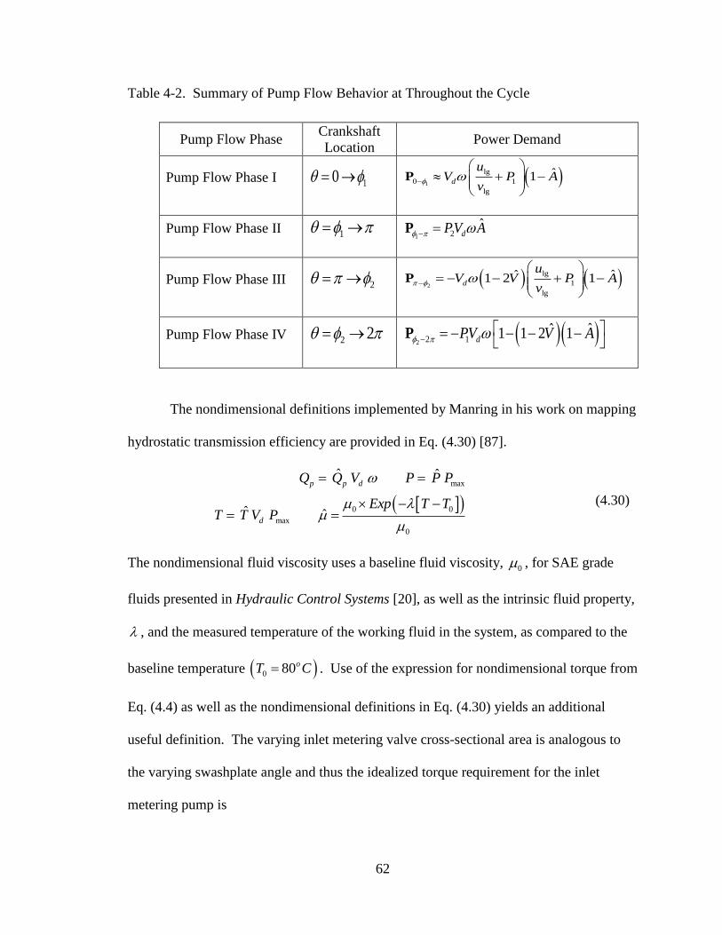
62
Table 4-2. Summary of Pump Flow Behavior at Throughout the Cycle
Pump Flow Phase Crankshaft
Location Power Demand
Pump Flow Phase I 10 1
lg
0 1
lg
ˆ1d
uV P A
v
P
Pump Flow Phase II 1 1 2
ˆdPV A P
Pump Flow Phase III 2 2
lg
1
lg
ˆˆ1 2 1d
uV V P A
v
P
Pump Flow Phase IV 2 2 2 2 1
ˆˆ1 1 2 1dPV V A
P
The nondimensional definitions implemented by Manring in his work on mapping
hydrostatic transmission efficiency are provided in Eq. (4.30) [87].
max
0 0
max
0
ˆ ˆ
ˆ ˆ
p p d
d
Q Q V P P P
Exp T TT T V P
(4.30)
The nondimensional fluid viscosity uses a baseline fluid viscosity, 0 , for SAE grade
fluids presented in Hydraulic Control Systems [20], as well as the intrinsic fluid property,
, and the measured temperature of the working fluid in the system, as compared to the
baseline temperature 0 80oT C . Use of the expression for nondimensional torque from
Eq. (4.4) as well as the nondimensional definitions in Eq. (4.30) yields an additional
useful definition. The varying inlet metering valve cross-sectional area is analogous to
the varying swashplate angle and thus the idealized torque requirement for the inlet
metering pump is

63
2ˆ
ideal dT V AP . (4.31)
There will also be an additional shaft power requirement associated with the vaporization
of the fluid. This requirement can be found by summing the power demands from Table
4-2 and yields
lg
lg
ˆ ˆ1 2vaporization d
uT V A V
v
. (4.32)
It is assumed that the inlet metering valve system will experience losses similar to those
depicted in the axial piston pump analysis. Thus, the entire torque requirement can be
written as
lg
2
lg
2
ˆ ˆ ˆ1 2
ˆ Exp ,ˆ ˆ
d d
p p
d p p p p
uT V A P V A V
v
V A P A B C DAP AP
(4.33)
where the coefficients Ap, Bp, Cp, and Dp in Eq. (4.33) come from the inlet metering valve
system experiments.
In order to nondimensionalize Eq. (4.33), the nondimensional grouping
lg
max lg
u
P v (4.34)
will be used in addition to the nondimensional groups already given in Eq. (4.5).
Equation (4.33) can be rewritten as Eq. (4.35).
2
ˆˆˆ ˆ ˆ ˆˆ ˆ ˆ ˆ ˆ ˆ ˆ2 1ˆ ˆp p p pT AP V A A APExp B C AP DAP
(4.35)

64
In Eq. (4.35) the first term encapsulates the ideal torque, and the second term contains the
additional torque required to vaporize and compress the fluid. The remaining terms
pertain to the energy losses that result from the typical use of a pump.
Recall from Eq. (3.26) that
2,ˆ ˆ
idealQ A . (4.36)
This derivation was based on an idealized pump performance. In order to account for the
inevitable leakage that will occur during operation of the single piston pump, loss
coefficients analogous to those identified in Eq. (4.3) and quantified in Table 4-1 will be
applied to Eq. (4.36). The pump volumetric flow rate, accounting for leakage losses, out
of the fixed displacement piston pump can be written as
2 0 1 2
ˆˆ ˆ ˆ ˆ ˆˆ ˆ
ˆ
PQ A K A P K K P
. (4.37)
The efficiency originally written in Eq. (4.1) can be rewritten in terms of Eqs. (4.35) and
(4.37) as Eq. (4.38).
0 1 2
0 0
ˆˆ ˆˆ ˆ ˆˆ ˆ
ˆ
ˆˆˆ ˆ ˆ ˆ ˆˆ ˆ ˆ ˆ ˆ ˆˆ2 1ˆ ˆp p p p
PP A K A P K K P
AP Q P V A A APExp B C AP DAP
(4.38)
Two additional nondimensional parameters,
0 0ˆ
dQ Q V and 0 0ˆ
ssP P P , (4.39)
are employed. The addition of the system inlet power to the denominator of Eq. (4.38) is
a result of the increased inlet pressure necessary for inlet metering system operation. For
operation of an axial piston variable displacement pump, the inlet pressure is simply
atmospheric pressure. This value is so small relative to the outlet pressure that it is

65
neglected. In contrast, the charge pump pressure is elevated over atmospheric pressure
and thus requires a greater energy input. From this point we can infer that it would be
prudent to keep the charge pressure, oP , as small as possible to maximize efficiency
while still providing a sufficient pressure drop across the valve to generate fluid
vaporization. The valve inlet volumetric flow rate, 0Q , is dependent on the charge pump
selection. A fixed displacement charge pump will always supply the maximum
volumetric flow rate 0ˆ 1Q ; however, a variable displacement charge pump could be
used to reduce the inlet flowrate requirement to a level proportional to the valve cross-
sectional area 0ˆ ˆQ A . The other differences between the efficiency in Eq. (4.6) and
Eq. (4.38) are the use of swashplate angle in the axial piston pump evaluation as
compared to the use of the inlet metering valve cross-sectional area as a means to control
the pump volumetric flow rate and the addition of the torque associated with fluid
vaporization in the denominator of Eq. (4.38).
In order to determine the experimentally derived leakage coefficients, the
measurements corresponding to the data collected for all inlet pressures (2.0, 2.5, 3.0, and
3.5 MPa), discharge pressures (2, 5, 10, 20, and 25 MPa), and two shaft speeds (1000 and
1500 rpm) were used. This data was collected by another research team, led by Dr.
Roger Fales, and discussion of the experimental methods employed is beyond the scope
of this dissertation. After these measurements were recorded, the torque, discharge flow
rate, and outlet pressure were averaged for each set outlet pressure and valve position
over the 10 second interval for which the valve was held in position. The relevant
averages were taken from the experimental measurements and then the Levenberg-

66
Marquardt algorithm was applied [89]. (The Appendix contains all the averaged data
employed throughout the analysis.)
The Levenberg-Marquardt algorithm is a numerical solution designed to minimize
a nonlinear function, such as the torque model in Eq. (4.35). This numerical approach
combines the steepest descent numerical method, which converges quite slowly but with
excellent stability, and the Gauss-Newton method, which converges on a solution rapidly,
but is prone to solution divergence [90]. Equation (4.40) shows the iterative equation
employed, and Fig. 4-5 illustrates the process.
1
1
T
k k k k k kw w J J I J e
(4.40)
In Eq. (4.40), w represents the “weights” or in our case, the coefficients (e.g. A,
B, C, and D). The Jacobian matrix, J, is derived from the matrix provided in Eq. (4.41) in
the search for coefficients A, B, C, and D, as well as the nondimensional thermodynamic
parameter . It is similarly derived from the matrix representation of Eq. (4.7) and
employed to determine the leakage coefficients K0, K1, and K2. Note that increasing the
combination coefficient, , decreases the step size, and decreasing the combination
coefficient increases the step size. This iterative adjustment of step size is what leads to
rapid solution convergence. The error is quantified in the term ke .
1 11 1 1 1 1 1 1
1 1 1 1 1
ˆˆˆ ˆ ˆˆ ˆ ˆ ˆˆ2 1 1ˆ ˆ ˆˆ ˆ
ˆˆ ˆˆˆˆ ˆ ˆˆ ˆ ˆ ˆˆ2 1 1ˆ ˆ
d d
d d
n n dnn nn n dn n dn n n
n dn
BV A A P Exp A P
A P T A PA
CT A PB
DV A A P Exp A PA P
(4.41)

67
Figure 4-5: Levenberg-Marquardt Solution Process [90]
The Levenberg-Marquardt solution process was applied to both the torque and
flow equations [Eq. (4.35) and (4.37)]. The resulting coefficients are provided in Table
4-3. Each of these coefficients has a physical meaning, as Eq. (4.35) and (4.37) are
models derived from the actual physical principles at work in operation of the inlet
metering pump.

68
Table 4-3. Inlet metering pump coefficients
Physical Meaning Symbol Value
Fluid compression 0 8.607E-02
Low Reynolds-number leakage 1 1.000E-02
High Reynolds-number leakage 2 5.063E-07
Static friction pA Effectively 0
Decay rate for boundary lubrication pB N/A
Hydrodynamic lubrication pC 1.305E-02
Starting torque pD 7.182E-02
Thermodynamic parameters 0.0140
These parameters yield a 2R value of 0.9822 with respect to flow evaluation, and a 2R
value of 0.9780 with respect to torque evaluation, suggesting that this method of
nonlinear coefficient determination is effective. The negligible magnitude of the static
friction coefficient, Ap, yields a slightly modified equation to describe the torque
requirement for the inlet metering system. The finalized model for torque, then, is
presented in Eq. (4.42), where the relevant coefficients are obtained from Table 4-3.
2ˆ ˆ ˆˆ ˆ ˆ ˆ ˆ ˆ2 1 p pT AP V A C AP D (4.42)
A comparison between Tables 4-1 and 4-3 yields insight into the operation of the
inlet metering pump. The effect of fluid compression, K0 is of the same magnitude in
operation of the two pumps. The working fluid in the two pumps was the same, and it
appears to have translated to the behavior of the fluid flow within the pump. Several

69
local minima exist which makes determining the leakage coefficients somewhat
challenging. After comparing multiple combinations of initial guesses and constraints
supplied to the iterative process used for solution, it was concluded that the result in
Table 4-3 yielded an excellent fit while simultaneously making physical sense. From this
result, we see that the high Reynolds number leakage is very near zero, but the low
Reynolds number leakage is of a similar magnitude to that of the variable displacement
pump [87].
Static friction was incredibly small for the inlet metering pump when compared to
the variable displacement pump. It is presumed that pump construction is the largest
contributing factor to this result. Operation of the variable displacement pump generates
substantial friction due to the metal-to-metal contact associated with its swashplate
position. In contrast, the inlet metering pump utilized a rolling element bearing for its
operation. From this, it was concluded that dropping the term containing the static
friction coefficient, A, would lead to the most physically appropriate model. This negated
a need to determine the decay rate for boundary lubrication, B. The hydrodynamic
lubrication, C, and starting torque, D, coefficients were both highly similar to the 145cc
variable displacement results.
One additional item of interest is the thermodyanamic parameter, , shown
earlier as Eq. (4.34). For all of the theoretical modeling conducted in this work, it was
assumed that the working fluid of the system was water ( =0.0298). Operation of the
experimental apparatus required use of CAT HYDO Advanced 10 hydraulic oil, a
proprietary hydraulic oil about which little is known in terms of thermodynamic
properties. The specific volume of the fluid is easily obtained [33], but the internal

70
energy is unknown. For this reason, the iterative process undertaken to determine the
other coefficients was also employed to estimate the thermodynamic property group
associated with the compression torque requirement. The magnitude of the
thermodynamic parameter determined for the inlet metering operating system is
comparable with that of water.
4.4 Efficiency Model Validation
The results presented in Table 4-3 were validated by evaluating the ability of the
efficiency model to predict the torque requirement and discharge flow for the pump’s
operation at higher shaft speeds. Data was taken for the pump operating at 2 MPa inlet
pressure, 2, 2.5, 5, 10, 20, and 25 MPa discharge pressure, and 2000 and 2500 rpm.
When these actual results were compared with the model predictions, the torque model
was found to have very good agreement with the higher speed data (R2 = 0.9835). The
flow model correlation coefficient was substantially lower (R2 = 0.7505); however, the
flow data associated with the higher pump speed operations showed significantly greater
variation than any of the other data recorded during pump operation. For comparison,
this information is presented in Table 4-4. Thus, it is assumed that the coefficients
associated with the flow model are reasonably good. Comparison of the new data with
the previously introduced model leads us to conclude that the model described by the
coefficients of Table 4-3 is valid.
Table 4-4. Standard Deviation of Collected Data
Standard Deviation of Averaged Flow at 1000 and 1500 rpm 0.2390
Standard Deviation of Averaged Flow at 2000 and 2500 rpm 0.3963
Standard Deviation of Averaged Torque at 1000 and 1500 rpm 0.2098
Standard Deviation of Averaged Torque at 2000 and 2500 rpm 0.2030

71
4.5 Discussion of the Variable Displacement and Inlet Metering System Analyses
In this chapter, governing equations describing the torque requirement and
discharge flow for the two pumps and their associated coefficients were presented. High
R2 values indicate that these coefficients provide reasonably good models for the
systems. These coefficients will be applied in Chapter 6 to facilitate further comparison
between the two designs, and actual measured efficiency values will also be presented.

72
CHAPTER 5. DESIGN AND MODELING
5.1 Introduction to System Design and Modeling
In this chapter a variety of numerical constraints will be developed. These
constraints will apply to the nondimensional groups presented in Chapter 3 and will be
used to aid the design process associated with the practical implementation of an inlet
metering valve system. Design requirements that will guarantee the system behaves in a
stable fashion will be introduced in Section 5.2. Additional design constraints will be
presented in Section 5.3. Application of these design constraints and the resulting
simplified model will be discussed in Section 5.4. Section 5.5 will analyze the dynamic
response of the system of equations, and Section 5.6 will illustrate our design process.
Section 5.7 will enumerate the sample systems that were designed for the purposes of our
study and assign numerical values to the constants that have been used throughout. A
discussion of our approach to modeling the behavior of this system will conclude the
chapter in Section 5.8.
5.2 System Stability
When the valve is disturbed from its initial resting state, it will either oscillate and
slowly return to its initial condition, or it will grow in oscillations until it fails or reaches
a physical limit. The desirable condition is for our valve to be stable, that is, to gradually
return to its initial resting state. We must determine if, in fact, our valve is stable. This
question of stability has been studied since 1856, when Hermite formally presented the
problem of finding the stability of a lumped parameter, linear, time-invariant system [93].

73
Gantmacher assesses Hermite’s solution as only partially complete; however, it was later
completely solved independently by both Routh and Hurwitz [94]. J. C. Maxwell was
also interested in the stability problem presented by Hermite. He was the first to publish
a dynamic analysis of a feedback system using differential equations in 1868, while
attempting to develop a speed governor [95]. In 1877 he served on a committee to
determine the winner of the Adams Prize, a prestigious award distributed by Cambridge
University to recognize original research in the field of mathematics [96]. This call for
papers was answered by E. J. Routh, who was awarded the Adams Prize for his essay on
the Stability of Motion [97, 98]. Routh’s paper showed that the number of roots in the
characteristic polynomial can be determined from the coefficients of the polynomial [98].
Eighteen years later, Hurwitz solved what was essentially the same problem. He was
working on controlling the speed of a high pressure water turbine, and was unaware of
the work done by Routh [99]. Their results are known collectively as the Routh-Hurwitz
stability criterion.
The Routh-Hurwitz stability criterion provides an algebraic procedure for
determining if the polynomial has any zeros in the right half plane [100]. If zeros exist in
the right half plane, the system is unstable. The zeros of the polynomial only lie entirely
in the left hand plane when a particular set of algebraic combinations of the coefficients
have the same sign [101]. A practical description for the application of the Routh-
Hurwitz criteria can be found in a variety of control texts, including Hydraulic Control
Systems by Noah Manring [20].
While the proof of the Routh-Hurwitz problem has existed since the late 1800’s,
considerable attention was lavished on the stability criterion in the 1990’s. The proofs

74
offered by Routh and Hurwitz both rely on advanced math techniques [98, 99], but in
1990 Chapellat et al applied the Hermite-Biehler theorem to stability criterion [102].
Since then, the academic community has produced multiple efforts to prove the Routh
Hurwitz criteria by elementary means in order to make the stability proof more accessible
to undergraduate students [103, 104]. While these proofs are valuable for deeper
understanding, ultimately we are concerned with practical application, and the coverage
in a standard control text [100] proves sufficient for the analysis conducted here.
The classic Routh-Hurwitz stability criterion can be used to consider system
stability. The Routh Hurwitz stability criteria will be applied to the nondimensional
equations presented as Eq. (3.51) in Chapter 3 of this work. Equation (3.51) is presented
in state space form here:
1 1
2 2
ˆ ˆ ˆ ˆ1 0 1
ˆ ˆ0 0 1 0
ˆ ˆˆ ˆˆ 11
ˆ ˆ ˆ ˆ
P K P K
y y
y K y Kc
m m m m
. (5.1)
The characteristic equation is then derived from Eq. (5.1) as follows:
1
2
ˆ 1 0 1 0 0
det 0 0 1 0 1 0 0
ˆ 0 0 1ˆ1
ˆ ˆ ˆ
K
s
K c
m m m
, (5.2)
where the resulting characteristic equation can be written as
3 2
2 1 2ˆ ˆ ˆˆ ˆ ˆ ˆ 0ms m c s c K s K K . (5.3)

75
For the system to be stable, the design criterion given by Eq. (5.4) must be
satisfied. Additionally, all the nondimensional groups must be real and positive values.
This will always be true given practical real world constraints, so this second requirement
will not be discussed further.
2 1 2ˆ ˆ ˆˆ ˆ ˆ ˆm c c K m K K (5.4)
Expansion of the terms in Eq. (5.4) reveals that neglecting the drag coefficient without
neglecting valve mass will always yield an unstable system. We can also observe from
Eq. (5.4) that the damping effects associated with the drag coefficient contribute to
stability. A third observation from Eq. (5.4) suggests that increasing the spring constant,
2K , will always increase system stability.
The most significant observation associated with Eq. (5.4) relies on the assertion
in Chapter 3 that the nondimensional leakage coefficient 1K is unity. If this design
criteria is applied to Eq. (5.4), we can see that the system will always be stable as long as
the coefficients are real and positive, which they must be. Thus, our system design will
always be stable.
5.3 Design Criteria Development
The stability criterion given in Eq. (5.4) provides the first guideline useful in the
design process. In order for the nondimensional leakage coefficient to be unity, the
design criteria shown in Eq. (5.5) must be satisfied.
max 0 02
ssss
d l
KPy
c y v P (5.5)

76
The maximum value of the valve displacement, maxy , can also be derived from the
equations that come from the analysis in Chapter 3. By setting Eqs. (3.27) and (3.29)
equal to each other, and recalling the nondimensional definitions in Eq.(3.8), we can
show
max 0 0 1
max
ˆ2 1
ˆ2 1d l d
p
vxy c v P P y V
A rvx
V
. (5.6)
We can solve Eq. (5.6) and find the maximum valve opening dimension to be as defined
as
max
0 02
d
d l
Vy
c v P
. (5.7)
This maximum valve displacement is a function of the pressure supplied by the charge
pump, 0P . Recall from the efficiency analysis in Chapter 4 that significant system
inefficiencies result from an elevated pressure at the charge pump outlet, and thus 0P
should be kept as small as possible (but still higher than the saturation pressure, 1P , of
the working fluid) while permitting reasonable design dimensions for the valve.
The mass of the valve can be designed by considering the dimensions of the
cross-sectional valve area, valveA , and the length of the valve, L , as well as the
anticipated valve material density (
). This result is shown in Eq. (5.8).
(5.8)

77
An additional design criteria can be derived from consideration of the
nondimensional spring constant coefficient. In order to minimize the spring preload
requirement,
1ss
valve ss
ky
A P . (5.9)
The spring preload force requirement can be evaluated using
2preload ss ss valveF k y P A (5.10)
to check for a reasonable magnitude.
The damping coefficient is also designed in terms of the valve dimensions. It is
calculated by
0.02
43 2 05
valveALc
E
. (5.11)
The origins of Eq. (5.11) can be found in published hydraulic texts [20].
Further, the system dynamic response is governed by the time scale, , which is
scaled by
2V
K
. (5.12)
Interestingly, the dynamic response is improved by increasing the system leakage.
Increased system leakage will also have a negative impact on the system efficiency. A
balance must be struck between achieving a fast time response while minimizing energy
losses. The time response can also be improved by increasing the volume of fluid at the
pump outlet.

78
The final design criteria that can be developed relies on the nondimensional
groups from Eq. (3.51). If the nondimensional spring constant coefficient, 2K , is several
orders of magnitude greater than the nondimensional mass coefficient, m , and the
nondimensional damping coefficient, there can be a highly useful dynamic result.
Equation (5.13) compares the expanded nondimensional spring constant [originally
defined in Eq. (3.49)] to, first, the nondimensional mass constant [defined in Eq. (3.49)],
and then to the nondimensional damping constant [defined in Eq. (3.49)]. The factor of
100 has been introduced to require that the nondimensional spring constant be several
orders of magnitude greater than the nondimensional mass and damping coefficients.
2
2
2 1
100
100
ss v ss
valve ss valve ss
ss ss
valve ss valve ss
k y m y
A P A P
k y c y
A P A P
(5.13)
Simplification of Eq. (5.13) yields the additional design criteria,
2
2
2
1
100
100
v
k
m
k
c
. (5.14)
These design criteria are notable because they enable a reduction of the order of the
nondimensional dynamic equations [see Eq. (3.51)]. The parameters in Eq. (5.14) can be
satisfied using physically reasonable design criteria. If this is done, the insignificant
terms in Eq. (3.51) can be neglected. We then find the simplified system of equations
which describes our system. This is shown here:

79
2 2
ˆ ˆ ˆ1. P
ˆ ˆ ˆˆ2. 1
P y
K y P K
. (5.15)
Equation (5.15) contains a significant result. We have developed a first order pressure
control system. This is different from a typical variable displacement pump design,
which is a second order system [105]. Equation (5.15) can be solved by hand; this will
be done in Section 5.4. This will enable “back of the envelope” calculations, and ease the
design process. These design criteria, as well as the stability criteria introduced in
Section 5.2, will be helpful to engineers who seek to develop and implement this
technology.
5.4 Solution of the System of Equations
The simplified system of equations given by Eq. (5.15) can be solved by hand
using basic differential equation solution techniques [106]. This solution is given in Eq.
(5.16).
2
2
2
2 2
ˆ1ˆ ˆ1 expˆ
ˆ11ˆˆ exp 1
ˆ ˆ
KP t
K
Ky t
K K
(5.16)
Examination of Eq. (5.16) illustrates the effects of changing the nondimensional spool
spring rate coefficient, 2K on the behavior of the system output pressure and valve
position.
While solution of Eq. (5.15) was relatively simple, the full dynamic set of
equations, provided at the conclusion of Chapter 3, cannot be solved by hand. Instead, it
80
must be solved numerically. The use of Eq. (5.16) is convenient; however, it is important
to make sure this simplified solution is equivalent to the results indicated by the full
system. In Chapter 6, a comparison of the simplified model and the full order model will
be made. At that point, we will be able to determine the ability of Eq. (5.16) to actually
describe our system behavior.
5.5 Dynamic System Response
A variety of information about the behavior of the valve can be derived from the
dynamic equations found in Chapter 3 of this work. The bandwidth frequency, bw , and
time constant, , can be found using Eqs. (5.17) through (5.21) [20].
The bandwidth frequency for the higher order system is the dynamic response
characteristic we are most interested in. The transfer function of the higher order system
is
2
3 2
2 2
ˆ1ˆˆ ˆˆ ˆ ˆ ˆ 1
KP s
ms m c s c K s K
, (5.17)
and the nondimensional bandwidth frequency can be found by numerically evaluating the
frequency where the amplitude of
2
3 2
2 2
ˆ1ˆˆ ˆˆ ˆ ˆ ˆ 1
KP j
mj m c c K j K
(5.18)
is equal to 22 . This solution must be determined numerically. The bandwidth
frequency for a first order system is also relevant, as it will apply to our simplified

81
models. The first order bandwidth frequency, in hertz, can be evaluated based on the
nondimensional pressure rise rate equation,
2
1 ˆ ˆ 11
1ˆ
P P
K
. (5.19)
Based on Eq. (5.19), the nondimensional bandwidth frequency is
2
1ˆ 1
ˆbw bwK
. (5.20)
This result is in radians. Thus, the first order bandwidth frequency in hz is evaluated as
2 2
1 11
ˆ 2bw
K
V K
(5.21)
and is a much more simple calculation than the numerical solution required by Eq. (5.18).
It can be completed quickly without the use of a computer.
Equations (5.18) and (5.21) give the maximum frequency of the pressure at
which the system output of the pressure will sufficiently track the input behavior of a
third and first order system respectively [20]. We are interested in the inlet metering
valve’s ability to control the downstream pressure output, and thus the higher the
bandwidth frequency, the more rapidly our inlet metering system will be able to respond
to pressure fluctuations. Similarly, a lower time constant will be desirable in generating
rapid system response. Further evaluation of the system bandwidth frequencies will
occur in Section 5.8 and Chapter 6.

82
5.6 Design Process
For the purposes of exploring the dynamic behavior of our system, we will
examine two different high order systems (Models A and B) based on Eq. (3.51) and two
simplified systems (Models A’ and B’) based on Eq. (5.15). While the process to arrive
at each of these systems is not difficult, many parameters are interrelated, and thus, a
thorough explanation of the design process will be introduced here.
All of the stability and design criteria [Eqs. (5.4) through (5.14)] rely on the
parameters encompassed by the four nondimensional groups 1 2ˆ ˆ ˆ ˆ, , , K K c m and the time
constant, . Some of these parameters are fixed based on the working fluid selection,
some of the values are products defined by other parameters, and the remaining values
are design parameters which we are free to choose, subject to reasonable physical
constraints. Table 5-1 explicitly lists the parameters and the amount of control designers
retain over them.
Table 5-1. Design parameters
Fluid Properties
(Fixed Value) Design Choice
(Free to Choose) Product of Design Choices
(Result of Third Column)
maxP dV ssP maxQ K
lv oP max
pA r
V maxy mv
lgv 2V Avalve ssy k
L Apump C
cd
In order to satisfy the stability and design criteria, the designer can select the
parameters listed as Design Choices. Selection of these values will impact the

83
magnitudes of the nondimensional groups. The relative magnitudes of the
nondimensional groups can be compared according to Eqs. (5.4) and (5.14) to determine
system stability and the relevance of the first order model to our higher order system.
Additionally, the equations describing the system dynamic response [Eqs. (5.17) through
Eq. (5.21)] can be used to predict certain aspects of our design’s response.
5.7 Illustrative Model Selection
Four models have been selected to explore the behavior of the inlet metering
system. These models have been selected to illustrate the variations in system behavior
as a result of differences in nondimensional group sizing. These models will be called
Model A, Model A’, Model B, and Model B’. Table 5-2 contains the design parameters
associated with the two baseline models based on Eq. (3.51). The models denoted with a
prime are the simplified models based on the design criteria given in Eq. (5.14) and the
resulting dynamic equations given by Eq. (5.15). Model A’ is the first order model of the
full order system represented by Model A. Similarly, Model B’ is the first order model of
the full order system represented by Model B.

84
Table 5-2. Model design parameter selections
Parameters Model A Model B Units
dV 3.33E-03 3.33E-03 m3/s
L 6 6 cm
mv 3.70E-02 1.33E-02 kg
K 363 48.4 kN/m
cd 0.62 0.62
Avalve 7.85E-05 2.83E-05 m2
c 0.628 0.377
max
pA r
V
0.10 0.10
maxQ 3.33E-03 3.33E-03 m3/s
maxy 10.9 4 mm
ssy 0.81 2.21 mm
ssP 15 15 MPa
K 1.67E-11 1.67E-11 m4s/kg
oP 0.10 0.10 MPa
maxP 20 20 MPa
lv 1.04E-03 1.04E-03 m3/kg
lgv 1.67 1.67 m3/kg
2.20 2.20 GPa
Models A, A’, B, and B’ will be compared with the variable displacement pump
introduced in Section 3.15. The numerical values associated with the nondimensional
groups in Eqs. (3.52) and (3.53) are provided in Table 5-3.
Table 5-3. Numerical values associated with the nondimensional parameters in Eq.
(3.52) [105]
Nondimensional Group Numerical Value
1 9.85E-02
1 88.03
2 2.934

85
Table 5-4 shows the numerical values of the nondimensional parameters and
differentiating characteristics of each of the models discussed in Chapter 5. These values
are the results of Eqs. (3.49) and (3.51), as well as Eqs. (5.4) and (5.14). It also provides
the dynamic characteristics found using Eqs. (5.17) through (5.21).
Table 5-4. Models of interest and their associated dynamic characteristics
Model A Model A’ Model B Model B’ Variable
Displacement
Stable Yes Yes Yes Yes Yes
[ms] 27.3 27.3 20.6 20.6 29.7
1K 1.00 1.00 1.00 1.00 N/A
2K 0.253 0.253 1.00 1.00 N/A
c 4.64E-04 0 1.74E-03 0 N/A
m 3.44E-05 0 1.63E-04 0 N/A
ˆbw 4.99 4.94 5.08 4.85 14.33
bw [hz] 29.14 28.82 39.19 37.41 76.87
Examination of Table 5-4 permits a preliminary understanding of the behavior of the inlet
metering system. Models A’ and B’ are not governed by Eqs. (5.17) or (5.18). Those
equations are only relevant for the higher order systems; instead, Models A’ and B’ are
the first order systems described by Eq. (5.15). Their first order nature is emphasized by
the “zero” value applied to the values of their nondimensional damping coefficient, c ,
and nondimensional mass coefficient, m . Observe that although Models A’ and B’ are
simplified approximations of the true system response described by Models A and B, the
first order model frequency calculation given by Eq. (5.21) results in only 0.9% relative
error between Models A and A’ and 4.3% relative error between Models B and B’.
Models A and A’ adhere to the design criteria developed in Section 5.3. Observing a

86
relative error of less than 1% in regards to the difference between the first order
bandwidth frequency response and the higher order bandwidth frequency response
indicates that Model A’ is indeed a good approximation of Model A. The ability to
quickly estimate the bandwidth frequency of the inlet metering design is an attractive
feature for engineers.
The four models described by the parameters in Table 5-4, as well the variable
displacement pump, will be modeled in Chapter 6, allowing us to gain further confidence
that the simplified models are reasonable approximations of the higher order models.
These models will solve Eqs. (3.51), (3.52), or (5.15) depending on their equations’
relevance to the model design based on the nondimensional parameters listed in
Table 5-3.
5.8 Modeling Introduction
As was mentioned earlier, the solution to the full dynamic set of equations
presented at the end of Chapter 3 cannot be found by hand. Instead, the solution must be
found numerically through the use of a computer driven solution. Modeling our system
in MATLAB/Simulink provides us with valuable insights in regards to how the system
will behave dynamically.
A block diagram of the dynamic system represented by Eq. (3.51), including all
terms whether significant or numerically insignificant (due to relatively small orders of
magnitude), is shown in Fig. 5-1. The simplified system [based on Eq. (5.15)] is shown
in Fig. 5-2. The system in Fig. 5-2 adheres to the design criteria developed in Section 5.3
of this work, and behaves in a first order fashion. Recall that the solution to Eq. (5.8) was

87
already found. It was provided as Eq. (5.9). Thus, it is unnecessary to actually solve the
first order model through use of the computer; however, it is convenient to solve Eq. (5.8)
by the same means as Eq. (3.51) purely for comparative efforts. The system models in
Figs. 5-1 and 5-2 will both be employed to solve Eqs. (3.51) and (5.15) respectively.
Figure 5-1. Block diagram of the full order inlet metering valve system

88
Figure 5-2. Block diagram of the reduced order inlet metering valve system
Comparison of Figs. 5-1 and 5-2 reveals that the introduction of the simplified
model permits removal of the higher order valve displacement terms. In the higher order
model, the valve position is controlled by the pressure P , the nondimensional mass
term m , the nondimensional damping coefficient c , and the nondimensional spring
constant coefficient 2K . In the simplified model, the valve position is only shaped by
the nondimensional spring constant. Figures 5-1 and 5-2 also show that there is no direct
change to the pressure behavior of the simplified model as compared to the higher order
model.
The results associated with modeling Eqs. (3.51), (3.52), and (5.8) will be
presented in Chapter 6 of this work. A discussion of these results and their physical
significance will also be presented in Chapter 6.

89
CHAPTER 6. RESULTS AND DISCUSSION
6.1 Results Introduction
This chapter will first present the experimental results and compare them with our
theoretical predictions. It will then present the results of the efficiency analysis presented
in Chapter 4. It will compare the efficiencies of the axial piston variable displacement
pump to the system efficiency of the inlet metering design. This comparison will first
employ the theoretical derivations and then present the efficiency measurements
associated with experimental results. It will then give the solutions to Eqs. (3.51) and
(5.8). These solutions vary with time, and plots of nondimensional valve displacement,
y , and nondimensional downstream pressure, P , as a function of nondimensional time,
t , will serve as a means to illustrate the results. Following the presentation of the system
dynamic behavior, a discussion of system stability will be conducted in Section 6.5.
Section 6.6 will be used to explore the importance of following the design criteria
presented in Chapter 5, and the final two sections of this chapter will compare the
dynamic response of the inlet metering system models that were developed to the
behavior of a variable displacement pump.
6.2 Experimental Results
The inlet metering system prototype introduced in Chapter 1 of this work was
employed to gather performance data that will be used to validate both the dynamic
equations developed in Chapter 3 as well as the efficiency predictions from Chapter 4.

90
For the experiments, the valve voltage supply was increased from 0 V to 0.5 V and then
from 1 to 5 V in 1 volt increments. This was done for the pressure and speed points listed
in Table 6-1. The valve voltage was adjusted at 10 second intervals. A hydraulic
schematic of the system was presented in Chapter 1, and a photograph of the actual setup
is presented as Fig. 6-1. Figure 6-2 shows the results for only one of the test conditions,
but it is representative of all results.
Table 6-1. Data Collection Points Associated with Experiments
Pump Inlet Pressure [MPa] Pump Outlet Pressures [MPa] Pump Shaft Speeds [rpm]
2.0 2.0, 5.0, 10.0, 20.0, 25.0 1000, 1500
2.5 2.0, 5.0, 10.0, 20.0, 25.0 1000, 1500
3.0 2.0, 5.0, 10.0, 20.0, 25.0 1000, 1500
3.5 2.0, 5.0, 10.0, 20.0, 25.0 1000, 1500
Figure 6-1. Inlet Metering System Experimental Set Up [107]

91
Figure 6-2. Volumetric flow rate over time for 2.5 MPa inlet pressure, 10 MPa
discharge pressure, 1500 rpm pump shaft speed
A variety of information can be derived from this recorded data. The pump
discharge flow rate as a function of valve cross-sectional area can be found and compared
with Eq. (6.1), which was derived in the analysis covered in Chapter 3.
2ˆ ˆQ A (6.1)
It is difficult to evaluate Eq. (6.1) by examination of Fig. 6-2. It is easier to see
the flow rate as a function of valve position if averages of volumetric flow rate at each
valve position are taken and plotted as a function of valve position. This result is shown
in Fig. 6-3. For these results, the data collected at a 2 MPa inlet pressure and 1500 rpm

92
shaft speed was averaged for all measured values of outlet pressure (2, 5, 10, 20, and 25
MPa) for a specified valve position.
Figure 6-3. Averaged nondimensional outlet flow as a function of measured valve
position
From Fig. 6-3 it can be seen that the volumetric flow rate and valve position
appear to be linearly related, similar to the prediction made by Eq. (6.1) for valve
positions of 0.5 to 2.0 V. For larger valve openings (from valve positions corresponding
to valve voltages of greater than 2.0 V), the valve position has no effect on the outlet
flow. From this, it is assumed that the experimental inlet metering valve is not sized in
the way our design suggests: where the maximum valve cross-section is the cross-section
at which fluid begins to vaporize and thus the pump outlet flow begins to be reduced by
any reduction in valve cross-sectional area. For the work presented in this dissertation,
all comparisons between our analytical predictions and the experimental results relies on

93
the assumption that the valve voltages of 2 – 5 V all correspond to the maximum valve
displacement ˆ 1A . Then, on the region between 0 and 2 V it appears that the flow out
of the fixed displacement pump varies linearly, as predicted by Eq. (6.1). In order to
consider this more deeply, let us consider the nondimensional expressions for the inlet
metering valve cross sectional area and the flow rate out of the pump which were derived
in the Chapter 3 analysis. For convenience, they have been rewritten here as Eqs. (6.2)
and (6.3).
ˆ ˆ ˆ2 1 2ˆ
ˆ1
V V vxA
vx
(6.2)
2
ˆˆ 1ˆ ˆ2 1
vxQ
V vx
(6.3)
Note that Eqs. (6.2) and (6.3) rely on the nondimensional terms for the piston volume, V ,
specific volume of the working fluid, v , and the fluid quality, x . In order for the direct
linear relationship between inlet metering valve opening and volumetric flow rate out of
the pump (shown in Eq. (6.1)) to be true, the fluid quality in Eq. (6.2) must be equal to
the fluid quality in Eq. (6.3) for all valve positions and flows. Solution of Eqs. (6.2) and
(6.3) for equivalent fluid qualities yields Eq. (6.4).
2
1ˆ ˆˆ2
Q AV
(6.4)
Recall the definition of the piston volume ratio in Eq. (3.8). The piston volume ratio, V ,
is 1
2 and thus, Eq. (6.4) matches the previously derived Eq. (6.1).
To evaluate the accuracy of the piston volume ratio prediction, a comparison of
the averaged volumetric flow rate as a function of nondimensionalized valve cross-

94
sectional area (on the region from 0 to 2 V) was plotted for each outlet pressure and
pump shaft speed. The pump inlet pressure appears to have had minimal effect on the
flow rate. Figures 6-4 and 6-5 show a comparison between the predicted Eq. (6.1) and
the averaged volumetric flow rate as a function of nondimensional valve cross-sectional
area for the measurements recorded for a 3 MPa inlet pressure.
Figure 6-4. Averaged non-dimensional pump outlet volumetric flow as a function of
nondimensional valve position for 3 MPa pump inlet pressure, 1000 rpm shaft speed
95
Figure 6-5. Averaged non-dimensional pump outlet volumetric flow as a function of
nondimensional valve position for 3 MPa pump inlet pressure, 1500 rpm shaft speed
These results demonstrate a good correlation between our prediction in Eq. (6.1)
and experimental results. Figures 6-4 and 6-5 show the results for the 3 MPa inlet
pressure, but this analysis can be conducted for all measured inlet pressure systems. A
comparison of the goodness of fit, as represented by R2 values, for the experimental
results depicted in Figs. 6-4 through 6-5 are provided in Table 6-2. These results were
consistent with the other inlet pressure measurement values: a nondimensional piston
volume ratio of 0.5 displays a reasonably good correlation with the results for shaft
speeds of 1000 and 1500 rpm, which aligns with the definition presented in Chapter 3.
Observe that the linear relationship between valve position and flow rate neglects leakage
losses. A better model will be presented in the upcoming sections of this work.
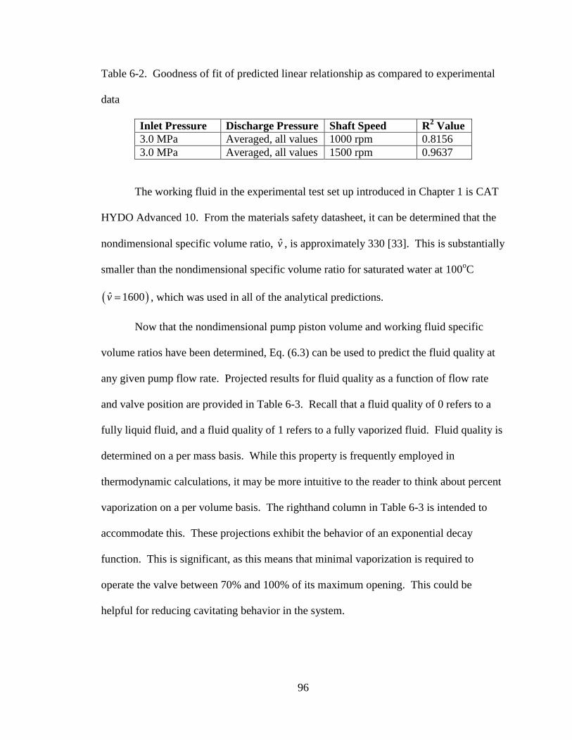
96
Table 6-2. Goodness of fit of predicted linear relationship as compared to experimental
data
Inlet Pressure Discharge Pressure Shaft Speed R2 Value
3.0 MPa Averaged, all values 1000 rpm 0.8156
3.0 MPa Averaged, all values 1500 rpm 0.9637
The working fluid in the experimental test set up introduced in Chapter 1 is CAT
HYDO Advanced 10. From the materials safety datasheet, it can be determined that the
nondimensional specific volume ratio, v , is approximately 330 [33]. This is substantially
smaller than the nondimensional specific volume ratio for saturated water at 100oC
ˆ 1600v , which was used in all of the analytical predictions.
Now that the nondimensional pump piston volume and working fluid specific
volume ratios have been determined, Eq. (6.3) can be used to predict the fluid quality at
any given pump flow rate. Projected results for fluid quality as a function of flow rate
and valve position are provided in Table 6-3. Recall that a fluid quality of 0 refers to a
fully liquid fluid, and a fluid quality of 1 refers to a fully vaporized fluid. Fluid quality is
determined on a per mass basis. While this property is frequently employed in
thermodynamic calculations, it may be more intuitive to the reader to think about percent
vaporization on a per volume basis. The righthand column in Table 6-3 is intended to
accommodate this. These projections exhibit the behavior of an exponential decay
function. This is significant, as this means that minimal vaporization is required to
operate the valve between 70% and 100% of its maximum opening. This could be
helpful for reducing cavitating behavior in the system.

97
Table 6-3. Predicted fluid quality as a function of nondimensional flow and valve
position
Nondimensional
Pump Outlet
Flow Rate 2Q
Nondimensional
Valve Position
A
Fluid Quality
x
Percentage of Fluid
that is Liquid by
Volume
0.1 0.1 2.73E-02 84.7%
0.2 0.2 1.21E-02 86.2%
0.3 0.3 7.07E-03 87.7%
0.4 0.4 4.55E-03 89.3%
0.5 0.5 3.03E-03 90.9%
0.6 0.6 2.02E-03 92.6%
0.7 0.7 1.30E-03 94.3%
0.8 0.8 7.58E-04 96.2%
0.9 0.9 3.37E-04 98.0%
1.0 1.0 0.00 100%
6.3 System Efficiency Results
In Chapter 4, extensive coverage was given to the derivation of the theoretical
models and associated coefficients for both the inlet metering system and the variable
displacement pump. Recall the derivation of the system efficiencies for both the axial
piston variable displacement pump and the inlet metering pump that took place in
Chapter 4. The axial piston variable displacement pump efficiency was written as
0 1 2
ˆˆ ˆ ˆˆ ˆ
ˆ
ˆˆˆ ˆ ˆˆ ˆ ˆ ˆˆ
ˆˆ
p
p
PP K P K K P
P A PExp B C P DP
, (6.5)
where is the normalized swashplate angle, P is the nondimensional pump discharge
pressure, is the nondimensional fluid viscosity and ˆp is the nondimensional pump
shaft angular velocity (This was previously introduced as Eq. (4.20) in the efficiency

98
analysis). The coefficients A, B, C, and D are experimentally derived constants. The
expression for the inlet metering pump efficiency differs in five ways:
1. The initial volumetric flow rate entering the inlet metering system must be
accounted for as it is transmitted at a pressure much higher than atmospheric
pressure.
2. Instead of a swashplate angle, the pump is controlled by the nondimensional
cross-sectional area, A .
3. There is an additional term in the denominator of the efficiency expression
associated with the torque required to vaporize the fluid.
4. Experimentation was done at a variety of shaft speeds, so the nondimensional
shaft speed, , cannot be uniformly treated as unity and thus excluded from the
efficiency equation. It must be considered.
5. Experimental results indicate that the static friction term (that is, the term
following the coefficient Ap) makes a negligible contribution to the behavior of
the system. This term can be neglected in the evaluation of the inlet metering
system.
The inlet metering pump efficiency in Eq. (6.6) makes use of new experimental
coefficients that were presented in Table 4-3.
0 1 2
0 0
ˆˆ ˆˆ ˆ ˆˆ ˆ
ˆ
ˆ ˆ ˆ ˆˆ ˆ ˆ ˆ ˆˆ2 1 p p
PP A K A P K K P
AP Q P V A C AP D
(6.6)
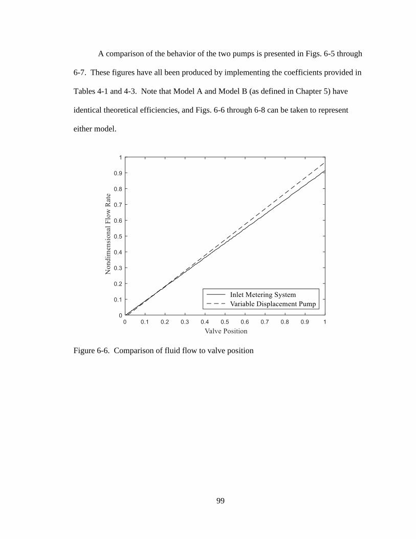
99
A comparison of the behavior of the two pumps is presented in Figs. 6-5 through
6-7. These figures have all been produced by implementing the coefficients provided in
Tables 4-1 and 4-3. Note that Model A and Model B (as defined in Chapter 5) have
identical theoretical efficiencies, and Figs. 6-6 through 6-8 can be taken to represent
either model.
Figure 6-6. Comparison of fluid flow to valve position

100
Figure 6-7. Torque requirement as a function of pump flow output
The idealized discharge flow rate of the pump, absent of leakage, would result in
a 45o line across Fig. 6-6. Leakage losses affect the inlet metering pump and variable
displacement pump differently. The flow output of the inlet metering pump is slightly
higher than the flow output of the variable displacement pump for low flow requirement
scenarios, but this changes quickly as the valve displacement increases, and for much of
the operational range of the two pumps, the inlet metering pump appears to be subject to
greater leakage losses. The torque requirement, illustrated by Fig. 6-7, is greater for the
inlet metering system than for the variable displacement pump for all flow rates. This is
due to the additional energy requirement associated with compressing the partially
vaporized fluid.

101
Figure 6-8. Pump efficiency as a function of pump flow output
Equation (6.6), coupled with the coefficients in Table 4-3, is plotted in Fig. 6-8
and shown with the solid line as the inlet metering system efficiency result. This
calculation takes into account the additional energy requirement associated with the
charge pump. Equation (6.5) and the coefficients in Table 4-1 provide the curve for the
variable displacement pump (indicated with the coarse dashed line). Equation (6.7) is
also applicable to studying the behavior of the inlet metering pump apart from the
additional charge pump energy requirement. This result is shown with the finely dashed
line, also in Fig. 6-8.

102
0 1 2
ˆˆ ˆˆ ˆ ˆˆ ˆ
ˆ
ˆˆˆ ˆ ˆˆ ˆ ˆ ˆˆˆ ˆp p p p
PP A K A P K K P
AP A APExp B C AP DAP
(6.7)
Figure 6-8 reveals the decreased efficiency of the inlet metering system. The primary
weakness of the inlet metering design is in its low efficiency.
Figure 6-9. Inlet metering pump efficiency map
Figure 6-9 contains the efficiency map for the inlet metering system design. This
mapping further emphasizes the decreased efficiency observed in operation of the inlet
metering pump as compared to previously published works [87, 107, 108]. Practitioners
may find this map useful in determining optimal operating points for the inlet metering
pump in the event that this design sees practical use.

103
Figure 6-10 presents the actual measured experimental data (as opposed to data
modeled using the experimentally derived coefficients), and compares the efficiency of
the inlet metering system for a variety of inlet and outlet pressures. The measurements
encapsulated in Fig. 6-10 were obtained for a range of inlet metering valve positions.
Figure 6-10. Measured efficiency results for the inlet metering system
Figure 6-10 reveals that the inlet metering system efficiency is largely impacted by the
discharge pressure selection. The inlet pressure, on the other hand, has minimal effect on
the system efficiency. The maximum measured efficiency for the inlet metering pump is
found to be 89.4%; however, once the charge system requirement is taken into account,
the inlet metering system maximum efficiency is recorded at 76.2%. The maximum
efficiency for a variable displacement pump is typically on the order of 85-95% [110].

104
6.4 A Qualitative Discussion about the Inlet Metering System Efficiency
Much of the analysis in this document disparages the efficiency of the inlet
metering system. The maximum efficiency of the inlet metering system is only 76.2%,
which is significantly lower than the maximum efficiency (94.1%) presented by the
variable displacement pump that serves as our consistent frame of reference throughout
this paper. Even when the inlet metering pump is considered apart from the charge pump
energy requirement, efficiency of the inlet metering pump never reaches 90%. However,
this negative comparison is not entirely fair.
It is important to keep in mind that we are comparing results from the operation of
two very different types of pumps. The variable displacement pump studied is a 145cc
model that can be purchased “off the shelf” for operation in a hydraulic system. The inlet
metering system pump is a 9 cc diesel fuel pump that was retrofit to operate in a
hydraulic system. The machining tolerances and construction of these two pumps are
very different. A more fair comparison might be represented by the result presented as
Fig. 6-11.

105
Figure 6-11. Normalized Efficiency Comparison
In Fig. 6-11 the efficiency of the variable displacement pump was normalized
about the maximum operating efficiency of the variable displacement pump that has been
studied throughout this paper, as shown in Eq. (6.8)
145
145
145
ˆmax
cccc
cc
(6.8)
Similarly, Eq. (6.9) shows how the inlet metering system and inlet metering pump were
both normalized about the maximum operating efficiency of the inlet metering pump.
ˆ
max
IMVsystem
IMVsystem
IMVpump
,
ˆ
max
IMVpump
IMVpump
IMVpump
(6.9)
The maximum operating efficiency of the inlet metering pump did not consider the
energy required by the charge pump. This consideration is reflected by the slightly

106
decreased efficiency of the inlet metering system (shown with the solid line) as compared
to the efficiency of the inlet metering pump on its own (shown with the finely dashed
line).
Examination of Fig. 6-12 suggests that the inlet metering system efficiency may
not be in as dire of shape as we had previously stated. If we were comparing identical
pump constructions, it appears that operation of the inlet metering system would still be
less efficient; however, the discrepancy between the traditional variable displacement
approach and the inlet metering approach is significantly smaller. This assertion is
clarified with Fig. 6-12.
Figure 6-12 Discrepancy Between the Normalized Efficiencies of the Variable
Displacement Pump and Inlet Metering System

107
The charge pump energy requirement means that, at minimum, the inlet metering
system is 2.4% less efficient than the variable displacement approach. This is
significantly less than the 18% decrease in efficiency predicted by Fig. 6-8. For
operating conditions at 60% or greater of the pump discharge flow rate, the inlet metering
system is less than 10% less efficient than the variable displacement pump. This loss in
efficiency may prove to be insignificant when the dynamic characteristics (which will be
presented in the following section) of the inlet metering system are considered.
6.5 Valve and Pressure Response Results
Our system is modeled in Matlab/Simulink based on the block diagrams from
Figs. 5-1 and 5-2. For all of the modeling simulations, it is helpful to note that the
simplified system (all models denoted with a prime) is denoted with a dashed line, and
the full order model (models denoted simply by a capital letter) is indicated with a solid
line. The simplified system was solved in Eq. (5.9) and can be plotted by hand in lieu of
solving it via a computing tool such as Matlab/Simulink. The higher order model (Eq.
3.51) cannot be solved by hand; however, and thus it necessitates our use of software.
Figs. 6-13 and 6-14 show the results for Models A and A’ and Figs. 6-14 and 6-15 show
the results for Models B and B’.

108
Figure 6-13. Models A and A’ valve displacement
Figure 6-14. Models A and A’ discharge pressure behavior
Model A
Model A’
Nondimensional Time, t
Nondim
ensi
onal
Pre
ssure
,
Nondimensional Time, t
Nondim
ensi
onal
Val
ve
Dis
pla
cem
ent,

109
Figure 6-15. Models B and B’ valve displacement
Figure 6-16. Models B and B’ discharge pressure behavior
Model B
Model B’
Nondimensional Time, t
Nondim
ensi
onal
Pre
ssure
,
Nondimensional Time, t
Nondim
ensi
onal
Val
ve
Dis
pla
cem
ent,
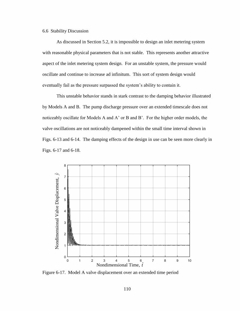
110
6.6 Stability Discussion
As discussed in Section 5.2, it is impossible to design an inlet metering system
with reasonable physical parameters that is not stable. This represents another attractive
aspect of the inlet metering system design. For an unstable system, the pressure would
oscillate and continue to increase ad infinitum. This sort of system design would
eventually fail as the pressure surpassed the system’s ability to contain it.
This unstable behavior stands in stark contrast to the damping behavior illustrated
by Models A and B. The pump discharge pressure over an extended timescale does not
noticeably oscillate for Models A and A’ or B and B’. For the higher order models, the
valve oscillations are not noticeably dampened within the small time interval shown in
Figs. 6-13 and 6-14. The damping effects of the design in use can be seen more clearly in
Figs. 6-17 and 6-18.
Figure 6-17. Model A valve displacement over an extended time period
Nondimensional Time, t
Nondim
ensi
onal
Val
ve
Dis
pla
cem
ent,

111
Figure 6-18. Model B valve displacement over an extended time period
6.7 Design Parameter Adherence
The design parameters provided as Eq. (5.7) have been selected in order to
guarantee that the relative order of magnitude of the nondimensional spring constant
coefficient is much greater than the nondimensional mass coefficient and the
nondimensional damping coefficient. If this is so, then the system can effectively be
modeled as a first order system as indicated by Eq. (5.9).
Models A and A’ obey the design criteria in Eq. (5.7); however, Models B and B’
do not. The significance of our design criteria development and findings is best
embodied by a comparison of Figs. 6-12 and 6-14: using this design, the inlet metering
pump can effectively produce a first order pressure response. Variable displacement
pumps display a second order pressure response [111]. The advantages associated with
the absence of pressure overshoot and oscillation may be significant, depending on the
Nondimensional Time, t
No
ndim
ensi
onal
Val
ve
Dis
pla
cem
ent,

112
application of this technology, and include reduction in system noise [112] and reduced
stress on design components. Evidence of efforts to minimize pressure overshoot cross
far-reaching industries, from biomedical applications [113] to residential well pumping
[114] to hydraulic applications [116, 117]. This system design, then, may have broad
application.
Figure 6-19. Magnified view of Models B and B’ pressure response
Figure 6-19 has been provided to show the magnitude of the higher order model’s
departure from the simplified first order model expressed as Model B’. From Fig. 6-19 it
can be seen that the simplified model never results in more than 10% error. As such, the
first order model may prove to be a convenient tool for back of the envelope calculations,
even when the design criteria developed in Eq. (5.7) are not adhered to.
Model B
Model B’
Nondim
ensi
onal
Pre
ssure
,
Nondimensional Time, t
113
6.8 System Dynamics Comparison
Evaluation of the system dynamics was first introduced in Chapter 5. Bode plots
will be employed in this section to compare the inlet metering system design to a variable
displacement pump (introduced in Section 5.6). The Bode plot was invented in 1938 by
Hendrik Bode, and combines two separate plots [117]. One plot depicts the magnitude of
the frequency response of the system, and the other shows the phase [118]. These figures
become a highly useful tool when analyzing the frequency response of a dynamic system.
As such, they will be applied here.
The Bode diagrams in Figs. 6-20 and 6-21 compare the dynamic response of the
full order inlet metering system (as described by the transfer function in Eq. (5.17), and
illustrated with a solid black line in the plots), the simplified inlet metering system (as
evaluated in Eq. (5.20) and illustrated with a dashed black line in the plots), and the
comparative variable displacement pump (described by the transfer function in Eq. (3.53)
and shown with a solid red line in the plots). Observe that the higher order model and
variable displacement pump both exhibit higher order response characteristics. This is
indicated by the slight overshoot. This occurs near a nondimensional bandwidth
frequency of 10 for the variable displacement pump, 30 for Model B, and 100 for Model
A. Note that the conversion from nondimensional frequency to a frequency in hertz is
ˆ
2
bwbw
. (6.8)
The simplified model bandwidth predictions of Models A’ and B’ exhibit first order
behavior, as expected. This is displayed as the straight dashed line followed by a drop off
on the Bode diagrams of Figs. 6-20 and 6-21.

114
Figure 6-20. Models A and A’ Bode Plot
Figure 6-21. Models B and B’ Bode Plot

115
Observe that the simplified system gives a reasonably good prediction of bandwidth
frequency for bandwidth frequencies of less than 200 hz (or near 35 on the
nondimensional plots). Because hydraulic systems rarely operate at frequencies above
even 25 hz, the simplified bandwidth calculations of Eqs. (5.20) and (5.21) are valid
design tools.
Further, observe that the higher order response values occur at greater frequencies
for the inlet metering system design than for the variable displacement pump design.
This means that for high speed hydraulic system designs that surpass 60 hz (e.g. electro-
hydraulically controlled injection machines in advanced manufacturing that can approach
200 hz [119]), our ability to delay the frequency at which the system experiences the
overshoot associated with the higher order response could be a valuable asset for high
speed applications.
The final notable characteristic of the dynamic response of the inlet metering
system can be shown in the step response plots provided in Figs. 6-22 and 6-23. Figure
6-22 compares Models A and A’ with the variable displacement pump model, and Figure
6-23 compares Models B and B’ with the same variable displacement pump model. Note
that for both inlet metering system designs, the inlet metering system shows negligible
pressure overshoot, while the variable displacement pump exhibits significant pressure
overshoot. It is desirable to minimize pressure overshoot, thus, the inlet metering system
design is attractive in this respect.

116
Figure 6-22. Models A and A’ Step Response Plot
Figure 6-23. Models B and B’ Step Response Plot

117
6.9 Discussion of Valve Dynamic System Response
The frequencies of our designs could present some issues associated with
thermodynamic flashing if the system undergoes phase change at a nonequilibrium rate.
Considerations of the thermodynamic modeling issues associated with flashing are
beyond the scope of this dissertation; however, work exists in the literature that suggests
that this issue is being considered by the academic community [119, 120]. It would be
valuable at some future point in time to conduct CFD simulations to gain greater insight
into the thermodynamic behavior of the system.
The efficiency comparisons presented in Figs. 6-7 and 6-8 reveal one of the main
limitations of the inlet metering system design: reduced efficiency. The normalized
efficiency comparison presented in Fig. 6-10 suggests, however, that the inlet metering
system may not represented a significant drop in efficiency, depending on the engineers’
goals for dynamic performance. This project would be greatly enhanced by a future true
head-to-head performance comparison, as well as design efforts focused on improving
the inlet metering system’s efficiency.
As discussed in Sections 6.7 and 6.8, one of the primary advantages associated
with the inlet metering system design is the ability to design a pump that produces a
discharge pressure governed by first order behavior. In contrast, the inlet metering valve
will always overshoot its designed steady-state valve position as the system approaches
its fixed steady-state outlet pressure. This does not present a physical issue as the
maximum valve displacement, which is a product of other design criteria (see Chapter 5
for more details), is several times greater than that of the steady-state valve displacement.
It does, however, point to another limitation of the first order model: it can only be used

118
to predict the behavior of the discharge pressure. The positioning of the inlet metering
valve cannot be exactly described by Eq. (5.9). Figures 6-17 and 6-18 illustrate this point
quite clearly.
Ultimately, our results show us that the inlet metering system results in a less
efficient pump design. However, this design results in a first order pressure response.
The controllability advantages associated with this may outweigh the energy costs of the
inlet metering system, depending on the application.

119
CHAPTER 7. CONCLUSION
7.1 Conclusion Introduction
This research initially set out to design a pump that could hold a constant
downstream pressure for a varying volumetric flow demand without requiring the use of
a variable displacement swashplate. Our goals in the pursuit of this design were to
improve pump efficiency and decrease system cost. As we developed the inlet metering
system design it became clear that we could shape the downstream pressure of the system
(and, in fact, get it to behave nearly according to a first order response, which
significantly improves upon the current second order pressure response associated with a
variable displacement pump) utilizing the inlet metering approach, thus satisfying our
original design criteria.
The inlet metering pump was initially proposed because of its anticipated
efficiency improvements. We expected the pump to require less torque to move the
partially vaporized fluid through the system (for a given volume we would be moving
less mass), which would decrease the amount of power that would need to be supplied.
However, our study revealed that the inlet metering approach was less efficient (about
70-90% efficient) when compared to the traditional variable displacement pump (about
95% efficient). Thoughtful consideration of the designs of the two pump considered
suggests that the efficiency discrepancy may not be as dire as suggested by these results
(see Section 6.4), but it is difficult to say for certain, as no data beyond that presented in
this dissertation is available.

120
As stated, cost considerations were another factor considered in this project.
Fixed displacement pumps are much cheaper than variable displacement pumps, and our
ability to design an inlet metering valve that permits the use of a fixed displacement
pump will definitely have a positive impact on the cost of manufacturing; however, our
investigation of the available literature has led us to recommend the installation of
cavitation-resistant inserts [29, 30, 33, 52]. This will increase the construction costs of a
fixed displacement pump; however, it seems protection against cavitation damage could
be prudent in light of the typical lifecycle and operation of a pump.
The biggest revelation that came from this theoretical analysis of the inlet
metering pump was that it could be designed to exhibit a first order pressure response.
We have noted in several places how unique this is when compared to a variable
displacement pump (e.g. [85, 105]). As long as both the design criteria and the Routh
Hurwitz stability criteria presented in Chapter 5 are satisfied, the simplified first order
solution (shown in Eq. 5.16) can accurately approximate the pressure behavior. The
ability to solve a system of dynamic equations that describe our pump system by hand
should ease the design process, as well as eliminate pressure overshoot and oscillation.
Following the construction of a theoretical model, a physical prototype was
constructed. Experimental data was obtained for assorted fixed inlet and outlet pressures,
as well as four different pump speeds. The information from these experiments was used
to determine the experimental coefficients, K0, K1, K2, A, B, C, and D that are used in the
estimation of downstream pressure and torque. These results were then applied to an
efficiency calculation, and we compared these projections to the calculated system

121
average efficiencies. Extremely good agreement (R2
> 0.97 for all predictions) was found
for both the flow and torque equations.
As the inlet metering system has been explored in the previous chapters, we have
found that we were able to satisfy our original design goal and learned a variety of things
about the anticipated behavior of the inlet metering system. Section 7.2 will present a list
of all conclusions drawn in this work. Section 7.3 will present a brief list comparing the
merits and drawbacks associated with the inlet metering design with the traditional
variable displacement pump. This dissertation will end with a discussion of the work to
be done on this topic for the future.
7.2 CONCLUSIONS
The following conclusions are supported by the analysis and results of this document:
1) Cavitation resistant inserts are recommended to mitigate the potential for pump
damage from the vaporization of the fluid [52].
2) Stainless steel or ceramic inserts are likely to be the most cavitation-resistant for a
water hydraulic system [29, 30, 33].
3) The theoretical prediction in regards to pump flow rate control is that there is a
direct linear relationship between the volumetric flow rate and valve cross-
sectional area.
4) A coupled set of equations, comprised of one first order differential equation and
one second order differential equation can be used to describe the inlet metering
valve and the discharge pressure of the single piston fixed displacement pump.

122
5) Nondimensionalization is an effective technique to compare the relative orders of
magnitude of the system parameters, and reveals that the valve mass and valve
damping coefficient have minimal impact on system dynamics.
6) Neglecting the insignificant terms in the coupled set of differential equations
yields a simplified first order system.
7) The simplified differential equations describing the inlet metering system can be
solved by hand, thus easing the design process.
8) For volumetric flow rates between 50 and 100% of the maximum pump outlet
flow rate, a 145cc pump (a representative variable displacement pump) exhibits
efficiencies ranging between 87 and 95%.
9) For volumetric flow rates between 50 and 100% of the maximum pump outlet
flow rate, the inlet metering pump yields a theoretical efficiency prediction
ranging between 77 and 83%.
10) For volumetric flow rates between 50 and 100% of the maximum pump outlet
flow rate, an inlet metering system yields a theoretical efficiency prediction
ranging between 72 and 81%.
11) The inlet metering valve system has additional power requirements of an elevated
valve inlet pressure and a vaporizing torque. These quantities both contribute to
the decreased efficiency of the inlet metering valve system.
12) Maintaining the minimum possible charge pump pressure requirement is
necessary to maximize the inlet metering valve system efficiency.

123
13) The inlet metering system will always result in a stable design as evaluated by the
Routh Hurwitz stability criterion if the system is designed such that the
nondimensional leakage coefficient 1K is unity.
14) Neglecting viscous drag without neglecting valve mass will always yield an
unstable system.
15) Viscous drag is a crucial stabilizing force in the operation of this valve.
16) Increasing the nondimensional spring constant, 2K , will always increase system
stability.
17) The dynamic response of the inlet metering system is improved by increasing the
system leakage.
18) Increasing the system leakage will have a negative impact on system efficiency.
19) Satisfaction of the design criteria supplied in Chapter 5 enables a system design
that adheres to first order pressure response.
20) Satisfaction of the design criteria supplied in Chapter 5 permits the use of a very
basic equation requiring only addition and the knowledge of the nondimensional
spring constant to estimate the bandwidth frequency of the inlet metering system.
21) Experimental results reveal that the volumetric flow rate and valve position are
linearly related for valve positions corresponding to 0 – 2.0 V, and volumetric
flow rate is unrelated for valve positions corresponding to 3.0 – 5.0 V.
22) The piston volume ratio V is approximately 0.5 for the inlet metering system
prototype.
23) The nondimensional specific volume ratio, v , is approximately 330 for the
working fluid in the inlet metering system prototype.

124
24) Fluid quality in the inlet metering system can be predicted utilizing equations
developed in this work.
25) A theoretical model for the efficiency of an inlet metering pump was developed.
26) The theoretical model for the inlet metering pump discharge flow rate shows
excellent correlation with experimental results for all measured values.
27) The theoretical model for the inlet metering pump torque requirement shows
excellent correlation with experimental results for all measured values.
28) System efficiency always increases for an increased discharge pressure.
29) System efficiency is not significantly changed by the inlet pressure.
30) The inlet metering system design is less efficient than the variable displacement
design for all flow rates.
31) The inlet metering system pressure response can be adequately predicted by the
simplified model if the design criteria from Chapter 5 are adhered to.
32) The inlet metering system can be designed such that the pressure exhibits a first
order response with negligible overshoot and oscillation if the design criteria from
Chapter 5 are adhered to.
33) The simplified system gives a reasonably good prediction of the inlet metering
system frequency for bandwidth frequencies of less than 200 hz.
34) The inlet metering system design delays the onset of higher order response from
about 70 hz (as occurs for the variable displacement pump modeled in this work)
to nearly 300 hz.
35) The inlet metering system exhibits minimal pressure overshoot, while the variable
displacement model exhibits significant overshoot.
125
36) The first order model can only be used to predict the behavior of the discharge
pressure. It fails to detail the valve oscillations.
37) An inlet metering valve combined with a fixed displacement pump can be used in
place of a variable displacement pump, thus introducing cost savings and
removing a mechanically complex piece of machinery.
7.3 Comparative Analysis
The following are considerations that suggest utilization of the inlet metering
valve system could display significant improvements over the traditional variable
displacement pump approach to flow control:
1. The inlet metering valve system eliminates the mechanically complex pieces
necessary for operation of a variable displacement swashplate
2. Fixed displacement pumps cost about 20% of the cost of a variable displacement
pump.
3. The inlet metering system can be designed such that the downstream pressure of
the pump displays a first order response.
a. The pressure from the inlet metering system does not exhibit overshoot
and oscillation.
b. The coupled set of differential equations that describes the inlet metering
system can be solved by hand, which simplifies the design process.
c. The simplified system of equations allows for a quick prediction of system
bandwidth frequency. It displays reasonably good accuracy and does not
require a numerical solution like that of the higher order system.

126
The following are issues that suggest the traditional variable displacement pump
approach retains advantages over the inlet metering approach to flow control:
1. The inlet metering approach ensures cavitation will occur in the hydraulic system.
a. Expensive erosion-resistant inserts may be required.
b. Cavitation driven noise could prove unappealing to consumers.
2. The inlet metering system consistently operates at efficiencies less than that of the
variable displacement pump for a given pump outlet flow.
3. Flashing and nonequilibrium thermodynamic issues are complex, could impact
the operation of this design, and require further investigation.
7.4 Future Work
The author is aware of the simplifications that were made in regard to the working
fluid in the inlet metering system. The simplicity of the assumption of pure water was
necessary for this preliminary work and is representative of contemporary approaches
found in the literature; however, it is not the most accurate depiction of realistic operating
conditions. If this work could be expanded to consider the thermodynamic properties of
hydraulic oil and account for the dissolved air that inevitably exists, that would mark a
considerable improvement in the modeling approach.
A Computational Fluid Dynamics (CFD) study of the valve and the phase change
occurring within the valve would provide valuable insight into the cavitation process, and
could expand the body of knowledge available to designers who are trying to implement
this technology. Further testing of the inlet metering system prototype could also provide
useful information. Evaluation of the long term effects of cavitation could provide
127
valuable insights on the potentially destructive results of fluid vaporization and the life of
the pump. This testing could aid designers in determining the importance and/or
placement of cavitation resistant inserts.
A second law thermodynamic efficiency evaluation, like the one developed by
Rakopoulos and Giakoumis that is discussed in Section 2.7, could supplement the first
order analysis that already occurred [70]. Exergy analyses are valuable for studying
individual components in the system, and could provide greater insight into both the
valve and pump independently. Further, exergy analyses are employed in optimization
activities [121, 124] and could be useful in design of inlet metering systems.
A final item that would be of great interest would be the experimental analysis of
a more directly comparable variable displacement pump and inlet metering system.
Figure 6-11 suggests that the efficiency losses associated with the inlet metering system
may be relatively small, and experimental validation of this assertion would be highly
valuable with respect to consideration of the marketability of the inlet metering design.
128
REFERENCES
[1] Gaudet, Timothy J. "Hydromechanical control for a variable delivery, positive
displacement fuel pump." ASME 1999 International Gas Turbine and Aeroengine
Congress and Exhibition. American Society of Mechanical Engineers, 1999.
[2] Taylor, Charles Fayette. (1985). Internal-Combustion Engine in Theory and Practice,
Volume 2 - Combustion, Fuels, Materials, Design (2nd Edition, Revised). (pp.
213-217). MIT Press.
[3] Gibson, W. H., and L. Fox. A New Development in High Speed Variable Delivery
Vane Pumps. No. 700792. SAE Technical Paper, 1970.
[4] Mathis, Christian. "Fuel injection system for an internal combustion engine." U.S.
Patent No. 4,884,545. 5 Dec. 1989.
[5] Hayes Jr, Edward James. "Fuel injector for internal combustion engines." U.S. Patent
No. 5,779,149. 14 Jul. 1998.
[6] de Ojeda, William, and Arturo Hern ndez. "Stability of a Pressure Compensated
Circuit For an Inlet Throttle Pump." ASME 2005 Fluids Engineering Division
Summer Meeting. American Society of Mechanical Engineers, 2005.
[7] Zhu, G-S., and Rolf D. Reitz. “Engine fuel droplet high-pressure vaporization
modeling.” Journal of engineering for gas turbines and power 123.2 (2001):
412-418.
[8] Ribbens, William. Understanding automotive electronics: an engineering
perspective. Butterworth-Heinemann, 2012.
[9] Stumpp, Gerhard, and Mario Ricco. Common rail-an attractive fuel injection system
for passenger car DI diesel engines. No. 960870. SAE Technical Paper, 1996.
[10] Heisler, Heinz. "Advanced engine technology." (1995). 594.
[11] Xin, Qianfan. (2011). Diesel Engine System Design. (pp. 467-469). Woodhead
Publishing.
[12] "Diesel fuel injector." U.S. Patent 3,072,114, issued January 8, 1963.
[13] Som, Sibendu, et al. "Effect of nozzle orifice geometry on spray, combustion, and
emission characteristics under diesel engine conditions." Fuel 90.3 (2011): 1267-
1276.
[14] Schweitzer, P. H., and Victor G. Szebehely. "Gas evolution in liquids and
cavitation." Journal of Applied Physics 21.12 (1950): 1218-1224.
[15] Atkins, Richard D.. (2009). An Introduction to Engine Testing and Development.
(pp. 68, 72). SAE International.

129
[16] Guerrassi, N., and P. Dupraz. A common rail injection system for high speed direct
injection diesel engines. No. 980803. SAE Technical Paper, 1998.
[17] Marčič, Milan. Optimization of the Diesel Engine Injection Nozzle. No. 932467.
SAE Technical Paper, 1993.
[18] Seabrook, Colin, and Clifford R. Burrows. "Water hydraulics- some design
challenges." AM SOC MECH ENG FLUID SYST TECHNOL DIV PUBL FPST 1
(1994): 59-63.
[19] Blackburn, John F., G. Reethof, and J. L. Shearer. "Fluid power control, 1960."
[20] Manring, Noah. Hydraulic control systems. Wiley, 2005.
[21] Lim, G. H., P. S. K. Chua, and Y. B. He. "Modern water hydraulics—the new
energy-transmission technology in fluid power." Applied Energy 76.1 (2003):
239-246.
[22] Fisher, J. "Water hydraulics getting hot again." Hydraulics & pneumatics 44.5
(1991): 35-38.
[23] Chua, Patrick SK, and F. L. Tan. "Experimental study of water hydraulics
application in aviation." Aircraft Engineering and Aerospace Technology 82.2
(2010): 91-98.
[24] Yang, Y. S., et al. "Water hydraulics-A novel design of spool-type valves for
enhanced dynamic performance." Advanced Intelligent Mechatronics, 2008. AIM
2008. IEEE/ASME International Conference on. IEEE, 2008.
[25] Shimizu, Seiji, and Atsushi Yamaguchi. "Cavitation erosion in hydraulic oil,
HWCFs, and tap water." Proceedings of the JFPS International Symposium on
Fluid Power. Vol. 1989. No. 1. 社団法人 日本フルードパワーシステム学会,
1989.
[26] Commission of the European Communities, “Fifth report on Specifications and
testing conditions relating to fire resistant fluids used for power transmission,”
Mines Safety Commission, Luxembourg, 1974.
[27] Basic Hydraulics and Components. Tokyo: Yuken Kogyo, 2006. Print.
[28] Urata, Eizo, et al. "Frequency response of a water hydraulic servovalve."Robotics
and Automation, 1995. Proceedings., 1995 IEEE International Conference on.
Vol. 3. IEEE, 1995.
[29] Urata, Eizo, et al. "Development of a Water Hydraulic Servovalve." JSME
International Journal Series B 41.2 (1998): 286-294.
[30] Trostmann E. Water hydraulics control technology. New York: Marcel Dekker
Inc.; 1996.
130
[31] Tan ACH. Water hydraulics in modern perspective: a 21st century clairvoyance. In:
Proceedings of International Conference on Production Research. Bangkok,
Thailand, 2000.
[32] Majdic, Franc, and Jozef Pezdirnik. "Oil-and water-based continuous control
valve." Industrial Lubrication and Tribology 62.3 (2010): 136-143.
[33] CAT HYDO Advanced 10; MSDS No. 32415; Exxon Mobil: Denver, CO,
September 5, 2007, http://www.catmsds.com/ (accessed March 12, 2015).
[34] Fitch, Ernest C., and I. T. Hong. Hydraulic system design for service assurance.
BarDyne, 2004.
[35] Caupin, Frédéric, and Eric Herbert. "Cavitation in water: a review." Comptes
Rendus Physique 7.9 (2006): 1000-1017.
[36] Mahulkar, A. V., et al. "Steam bubble cavitation." AIChE journal 54.7 (2008):
1711-1724.
[37] Tullis, J. Paul. Hydraulics of pipelines: pumps, valves, cavitation, transients. John
Wiley & Sons, 1989.
[38] HIBI, Akira, et al. "Suction Performance of Axial Piston Pump: 1st Report,
Analysis and Fundamental Experiments." Bulletin of JSME 20.139 (1977): 79-84.
[39] Thiruvengadam, A. The concept of erosion strength. No. TR-233-9.
HYDRONAUTICS INC LAUREL MD, 1965.
[40] Hattori, Shuji, Ryohei Ishikura, and Qingliang Zhang. "Construction of database on
cavitation erosion and analyses of carbon steel data." Wear 257.9 (2004): 1022-
1029.
[41] Hattori, Shuji, and Ryohei Ishikura. "Revision of cavitation erosion database and
analysis of stainless steel data." Wear 268.1 (2010): 109-116.
[42] Heymann, F. J. "Toward quantitative prediction of liquid impact erosion." ASTM
STP 474 (1970): 212.
[43] Varga, J. J. “Cavitation erosion and mechanical properties of materials.”
Proceedings of the Seventh Conference on Fluid Machinery. Vol 2. (1983) 911-
916.
[44] Arndt, Roger EA. "Cavitation in fluid machinery and hydraulic structures."Annual
Review of Fluid Mechanics 13.1 (1981): 273-326.
[45] Martin, C. Samuel, et al. "Cavitation inception in spool valves." Journal of fluids
Engineering 103.4 (1981): 564-575.
[46] IBUKI, Takao, et al. "Suction Performance of Axial Piston Pump: 2nd Report,
Experimental Results." Bulletin of JSME 20.145 (1977): 827-833.

131
[47] Suzuki, K., and E. Urata. "Development of a direct pressure-sensing pressure-
reducing valve for water hydraulics." Proceedings of the Institution of Mechanical
Engineers, Part I: Journal of Systems and Control Engineering 222.8 (2008):
787-797.
[48] Liu, Y. S., Huang, Y., and Li, Z. Y. Experimental investigation of flow and
cavitation characteristics of a two-step throttle in water hydraulic valves. Proc.
Istn Mech. Engrs. Part A: J. Power Energy, 2002, 216, 105-111.
[49] Manring, N. D. and Johnson, R. E. Optimal orifice geometry for a hydraulic
pressure-reducing valve. Trans. ASME, G, J. Dynamic System Measmt Control,
1997, 119(3), 467-473.
[50] Schiavello, Bruno, and Frank C. Visser. "Pump Cavitation—Various NPSHR
Criteria, NPSHA Margins, and Impeller Life Expectancy." Proceedings of the
25th International Pump Users Symposium, Turbomachinery Laboratory, Texas
A&M University, College Station, TX. 2009.
[51] Wang, Shu. "The analysis of cavitation problems in the axial piston pump."Journal
of Fluids Engineering 132.7 (2010): 074502.
[52] Knapp, Robert Talbot, James W. Daily, and Frederick G. Hammitt. "Cavitation."
(1979). 517.
[53] Kobus, Helmut. "Local air entrainment and detrainment." (1984).
[54] Merritt, Herbert E. Hydraulic control systems. John Wiley & Sons, 1967.
[55] S. Majtenyi, Mathematical Modeling of Cavitation in Hydraulic Pumps, IFAC
Pneumatic & Hydraulic Components, 1980, pp21-26.
[56] Cho, Baek-Hyun, Hyoun-Woo Lee, and Jong-Sun Oh. "Estimation technique of air
content in automatic transmission fluid by measuring effective bulk
modulus." International journal of automotive technology 3.2 (2002): 57-61.
[57] Watton, J., 1989, Fluid Power Systems: Modeling, Simulation, Analog and
Microcomputer Control, Prentice Hall, New York.
[58] Budris, Allen R., and Phillip A. Mayleben. "Effects of entrained air, NPSH margin,
and suction piping on cavitation in centrifugal pumps." PROCEEDINGS OF THE
INTERNATIONAL PUMP USERS SYMPOSIUM. TEXAS A&M UNIVERSITY
SYSTEM, 1998.
[59] Fowle, T. I. "Aeration in lubricating oils." Tribology international 14.3 (1981): 151-
157.
[60] Van de Ven, James D. "On Fluid Compressibility in Switch-Mode Hydraulic
Circuits—Part I: Modeling and Analysis." Journal of Dynamic Systems,
Measurement, and Control 135.2 (2013): 021013.

132
[61] Chanson, Hubert. "Study of air entrainment and aeration devices." Journal of
Hydraulic research 27.3 (1989): 301-319.
[62] Moran, Michael J., et al. Fundamentals of engineering thermodynamics. John Wiley
& Sons, 2010.
[63] Doolittle, Jesse Seymour. Thermodynamics for engineers. International Textbook
Co., 1964.
[64] Ahamed, J. U., R. Saidur, and H. H. Masjuki. "A review on exergy analysis of
vapor compression refrigeration system." Renewable and Sustainable Energy
Reviews 15.3 (2011): 1593-1600.
[65] Hasan, Afif Akel, D. Yogi Goswami, and Sanjay Vijayaraghavan. "First and second
law analysis of a new power and refrigeration thermodynamic cycle using a solar
heat source." Solar Energy 73.5 (2002): 385-393.
[66] Khaliq, Abdul, Basant K. Agrawal, and Rajesh Kumar. "First and second law
investigation of waste heat based combined power and ejector-absorption
refrigeration cycle." International Journal of Refrigeration 35.1 (2012): 88-97.
[67] Pridasawas, Wimolsiri, and Per Lundqvist. "An exergy analysis of a solar-driven
ejector refrigeration system." Solar energy 76.4 (2004): 369-379.
[68] Morosuk, T., and G. Tsatsaronis. "Advanced exergetic evaluation of refrigeration
machines using different working fluids." Energy 34.12 (2009): 2248-2258.
[69] Bi, Yuehong, et al. "Comprehensive exergy analysis of a ground-source heat pump
system for both building heating and cooling modes." Applied Energy86.12
(2009): 2560-2565.
[70] Rakopoulos, C. D., and E. G. Giakoumis. "Comparative first-and second-law
parametric study of transient diesel engine operation." Energy 31.12 (2006):
1927-1942.
[71] Bejan, A. Advanced Engineering Thermodynamics. Wiley, New York (1988).
[72] Keenan, Joseph Henry. "An investigation of ejector design by analysis and
experiment." Journal of Applied Mechanics 17 (1950): 299.
[73] Huang, B. J., et al. "A 1-D analysis of ejector performance." International Journal
of Refrigeration 22.5 (1999): 354-364.
[74] Ding, Guo-liang. "Recent developments in simulation techniques for vapour-
compression refrigeration systems." International Journal of Refrigeration 30.7
(2007): 1119-1133
[75] Bilicki, Zbigniew, and Roman Kwidziński. "Thermodynamic and mechanical
nonequilibrium in flashing flow with a shock wave in liquid-vapour
mixture."Journal of Theoretical and Applied Mechanics 35.2 (1997): 263-284.
133
[76] Wang, Jiangfeng, Yiping Dai, and Zhixin Sun. "A theoretical study on a novel
combined power and ejector refrigeration cycle." international journal of
refrigeration 32.6 (2009): 1186-1194.
[77] Atkins, Anthony G., Tony Atkins, and Marcel Escudier. A dictionary of mechanical
engineering. Oxford University Press, 2013.
[78] Munson, B. R., D. F. Young, and T. H. Okiishi. 1998. Fundamentals of Fluid
Mechanics, 3d ed. John Wiley & Sons, New York.
[79] Mises, R. v., “Berechnung von Ausfluss und Ueberfallzahlen,” VD1 Zeitschrift,
1917, pp. 447-462.
[80] Birkhoff, Garrett. Jets, wakes, and cavities. Elsevier, 2012.
[81] Schoenau, G. J., R. T. Burton, and G. P. Kavanagh. "Dynamic analysis of a variable
displacement pump." Journal of Dynamic Systems, Measurement, and
Control 112.1 (1990): 122-132.
[82] Manring, Noah D. "Sensitivity analysis of the conical-shaped equivalent model of a
bolted joint." ASME 2003 International Mechanical Engineering Congress and
Exposition. American Society of Mechanical Engineers, 2003.
[83] Johnson, Robert E., and Noah D. Manring. "Sensitivity studies for the shallow-
pocket geometry of a hydrostatic thrust bearing." ASME 2003 International
Mechanical Engineering Congress and Exposition. American Society of
Mechanical Engineers, 2003.
[84] Zeiger, G., and A. Akers. "Torque on the swashplate of an axial piston
pump." Journal of dynamic systems, measurement, and control 107.3 (1985):
220-226.
[85] Manring, Noah D., and Viral S. Mehta. "Physical limitations for the bandwidth
frequency of a pressure controlled, axial-piston pump." Journal of Dynamic
Systems, Measurement, and Control 133.6 (2011): 061005.
[86] Schoenau, G. J., R. T. Burton, and G. P. Kavanagh. "Dynamic analysis of a variable
displacement pump." Journal of Dynamic Systems, Measurement, and
Control 112.1 (1990): 122-132.
[87] Manring, Noah D. "Mapping the Efficiency for a Hydrostatic
Transmission."Journal of Dynamic Systems, Measurement, and Control 138.3
(2016): 031004.
[88] Heij, Christiaan, et al. Econometric methods with applications in business and
economics. OUP Oxford, 2004.
[89] Ranganathan, Ananth. "The Levenberg-Marquardt algorithm." Tutoral on LM
Algorithm (2004): 1-5.

134
[90] Yu, Hao, and Bogdan M. Wilamowski. "Levenberg-marquardt training."Industrial
Electronics Handbook 5 (2011): 12-1.
[91] Ho, Triet Hung, and Kyoung Kwan Ahn. "Modeling and simulation of hydrostatic
transmission system with energy regeneration using hydraulic
accumulator." Journal of Mechanical Science and Technology 24.5 (2010): 1163-
1175.
[92] Hofman, Theo, et al. "Design of CVT-based hybrid passenger cars."Vehicular
Technology, IEEE Transactions on 58.2 (2009): 572-587.
[93] Hermite, C., Sur le nombre des racines d'une ~quation algebrique comprise entre
des limites donnes, d. Reine Angew. Math., 51, 39-51, 1856.
[94] Gantmacher, F. R., The Theory of Matrices, Vol. 2, Chelsea, New York, 1959. Pgs
172-173.
[95] J.C. Maxwell, "On govemors," in Proc. Royal Society of London, vol. 16, pp. 270-
283, 1868.
[96] Maxwell, James Clerk. The Scientific Letters and Papers of James Clerk Maxwell:
1874-1879. Vol. 3. CUP Archive, 1990. Pg 6.
[97] Clark, Robert N. "The Routh-Hurwitz stability criterion, revisited." IEEE Control
Systems Magazine 12.3 (1992): 119-120.
[98] E.J. Routh, A Treatise on The Stability of Motion. London, U.K.: Macmillan, 1877.
[99] A. Hurwitz, "On the conditions under which an equation has only roots with
negative real parts," Mathematische Annelen, vol. 46, pp. 273-284, 1895.
[100] Shinners, Stanley M. Advanced modern control system theory and design. John
Wiley & Sons, Inc., 1998.
[101] Meinsma, Gjerrit. "Elementary proof of the Routh-Hurwitz test." Systems &
Control Letters 25.4 (1995): 237-242.
[102] H. Chapellat, M. Mansour, and S. P. Bhattacharyya, “Elementary proofs of some
classical stability criteria,” IEEE Trans. Educ., vol. 33, Aug. 1990.
[103] Anagnost, John Joseph, and Charles A. Desoer. "An elementary proof of the
Routh-Hurwitz stability criterion." Circuits, systems and signal processing 10.1
(1991): 101-114.
[104] Ho, Ming-Tzu, Aniruddha Datta, and S. P. Bhattacharyya. "An elementary
derivation of the Routh-Hurwitz criterion." Automatic Control, IEEE
Transactions on 43.3 (1998): 405-409.
[105] Manring, N. D., and R. E. Johnson. "Modeling and designing a variable-
displacement open-loop pump." Journal of dynamic systems, measurement, and
control 118.2 (1996): 267-271.
135
[106] Boyce, William E., Richard C. DiPrima, and Charles W. Haines. Elementary
differential equations and boundary value problems. Vol. 9. New York: Wiley,
1992.
[107] Manring, Levi. “Inlet Metering System Experimental Set Up.” 2016.
[108] Ho, Triet Hung, and Kyoung Kwan Ahn. "Modeling and simulation of hydrostatic
transmission system with energy regeneration using hydraulic
accumulator." Journal of Mechanical Science and Technology 24.5 (2010): 1163-
1175.
[109] Hofman, Theo, et al. "Design of CVT-based hybrid passenger cars."Vehicular
Technology, IEEE Transactions on 58.2 (2009): 572-587.
[110] Manring, Noah D. "Friction forces within the cylinder bores of swash-plate type
axial-piston pumps and motors." Journal of dynamic systems, measurement, and
control 121.3 (1999): 531-537.
[111] Manring, N. D., and R. E. Johnson. "Modeling and designing a variable-
displacement open-loop pump." Journal of dynamic systems, measurement, and
control 118.2 (1996): 267-271.
[112] Kim, Jong-Ki, et al. "Relation between pressure variations and noise in axial type
oil piston pumps." KSME international journal 18.6 (2004): 1019-1025.
[113] Newell, Scott W. "Inflation control apparatus for an automatic blood pressure
gauge." U.S. Patent No. 5,240,008. 31 Aug. 1993.
[114] Konrad, Charles E. "High speed deep well pump for residential use." U.S. Patent
No. 5,883,489. 16 Mar. 1999.
[115] Sakakibara, Satoshi, and Kenji Nakashima. "Hydraulic transmission control
system and method for vehicle having automatic engine stop/restart function."
U.S. Patent Application 10/886,612.
[116] Hwang, KyoungPil, Andrew D. Herman, and Michael Kozan. "Hydraulic
over/undershoot protection for transmission clutch control." U.S. Patent No.
7,850,572. 14 Dec. 2010.
[117] Bode, H. W. "Variable equalizers." Bell System Technical Journal 17.2 (1938):
229-244.
[118] Engelberg, Shlomo. A mathematical introduction to control theory. Vol. 2.
Imperial College Press, 2005.
[119] Chiang, Mao-Hsiung, Chung-Chieh Chen, and Chung-Feng Jeffrey Kuo. "The
high response and high efficiency velocity control of a hydraulic injection
molding machine using a variable rotational speed electro-hydraulic pump-
controlled system." The International Journal of Advanced Manufacturing
Technology 43.9-10 (2009): 841-851.

136
[120] Saha, P., N. Abuaf, and B. J. C. Wu. "A nonequilibrium vapor generation model
for flashing flows." Journal of heat transfer 106.1 (1984): 198-203.
[121] Kolev, Nikolay Ivanov. "Validation of multiphase flow models." Multiphase Flow
Dynamics 3. Springer Berlin Heidelberg, 2012. 425-666.
[122] Tsatsaronis, George. "Strengths and limitations of exergy
analysis."Thermodynamic optimization of complex energy systems. Springer
Netherlands, 1999. 93-100.
[123] Nuñez, M. Picon. "Exergy analysis and optimization of a solar-assisted heat
pump." Energy 23.4 (1998): 337-344.
[124] Yumrutaş, Recep, Mehmet Kunduz, and Mehmet Kanoğlu. "Exergy analysis of
vapor compression refrigeration systems." Exergy, an International Journal 2.4
(2002): 266-272.
[125] Wang, Sheng, and Shudong Wang. "Exergy analysis and optimization of methanol
generating hydrogen system for PEMFC." International journal of hydrogen
energy 31.12 (2006): 1747-1755.
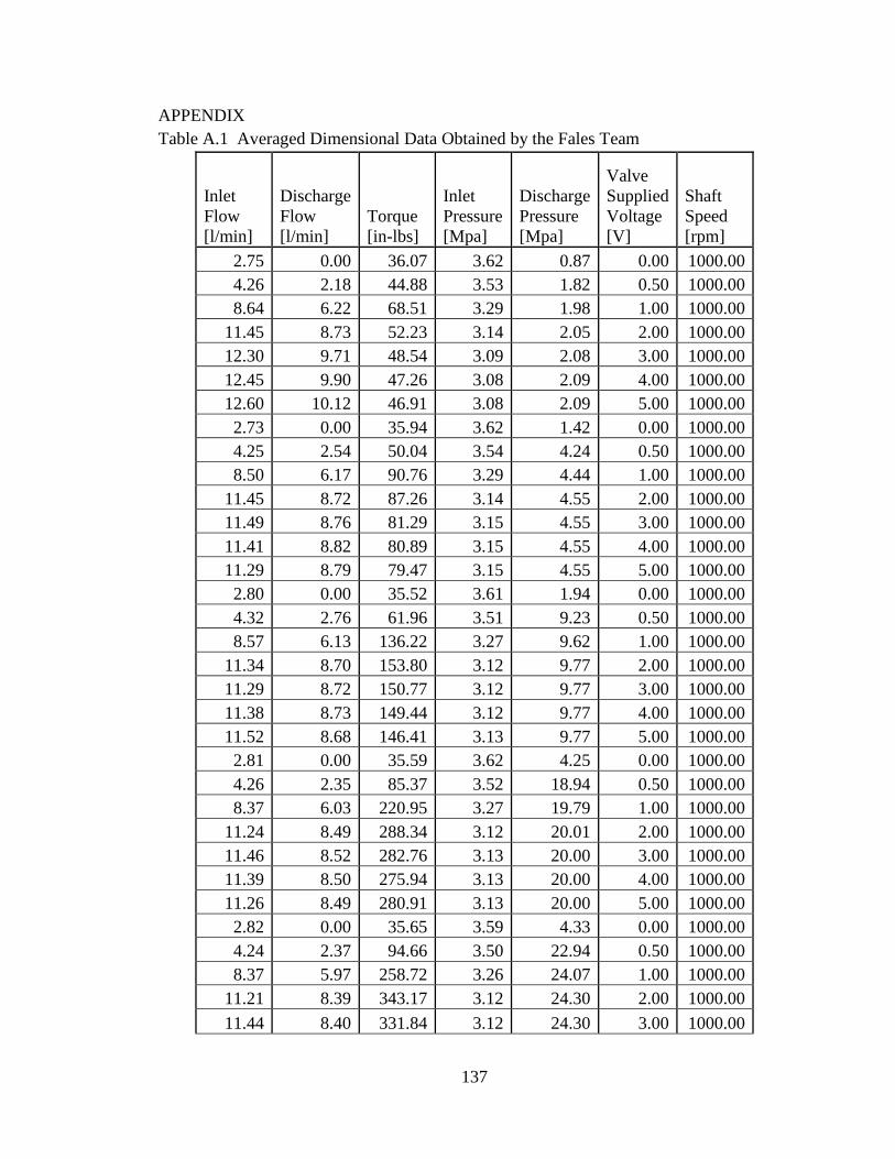
137
APPENDIX
Table A.1 Averaged Dimensional Data Obtained by the Fales Team
Inlet
Flow
[l/min]
Discharge
Flow
[l/min]
Torque
[in-lbs]
Inlet
Pressure
[Mpa]
Discharge
Pressure
[Mpa]
Valve
Supplied
Voltage
[V]
Shaft
Speed
[rpm]
2.75 0.00 36.07 3.62 0.87 0.00 1000.00
4.26 2.18 44.88 3.53 1.82 0.50 1000.00
8.64 6.22 68.51 3.29 1.98 1.00 1000.00
11.45 8.73 52.23 3.14 2.05 2.00 1000.00
12.30 9.71 48.54 3.09 2.08 3.00 1000.00
12.45 9.90 47.26 3.08 2.09 4.00 1000.00
12.60 10.12 46.91 3.08 2.09 5.00 1000.00
2.73 0.00 35.94 3.62 1.42 0.00 1000.00
4.25 2.54 50.04 3.54 4.24 0.50 1000.00
8.50 6.17 90.76 3.29 4.44 1.00 1000.00
11.45 8.72 87.26 3.14 4.55 2.00 1000.00
11.49 8.76 81.29 3.15 4.55 3.00 1000.00
11.41 8.82 80.89 3.15 4.55 4.00 1000.00
11.29 8.79 79.47 3.15 4.55 5.00 1000.00
2.80 0.00 35.52 3.61 1.94 0.00 1000.00
4.32 2.76 61.96 3.51 9.23 0.50 1000.00
8.57 6.13 136.22 3.27 9.62 1.00 1000.00
11.34 8.70 153.80 3.12 9.77 2.00 1000.00
11.29 8.72 150.77 3.12 9.77 3.00 1000.00
11.38 8.73 149.44 3.12 9.77 4.00 1000.00
11.52 8.68 146.41 3.13 9.77 5.00 1000.00
2.81 0.00 35.59 3.62 4.25 0.00 1000.00
4.26 2.35 85.37 3.52 18.94 0.50 1000.00
8.37 6.03 220.95 3.27 19.79 1.00 1000.00
11.24 8.49 288.34 3.12 20.01 2.00 1000.00
11.46 8.52 282.76 3.13 20.00 3.00 1000.00
11.39 8.50 275.94 3.13 20.00 4.00 1000.00
11.26 8.49 280.91 3.13 20.00 5.00 1000.00
2.82 0.00 35.65 3.59 4.33 0.00 1000.00
4.24 2.37 94.66 3.50 22.94 0.50 1000.00
8.37 5.97 258.72 3.26 24.07 1.00 1000.00
11.21 8.39 343.17 3.12 24.30 2.00 1000.00
11.44 8.40 331.84 3.12 24.30 3.00 1000.00

138
Inlet
Flow
[l/min]
Discharge
Flow
[l/min]
Torque
[in-lbs]
Inlet
Pressure
[Mpa]
Discharge
Pressure
[Mpa]
Valve
Supplied
Voltage
[V]
Shaft
Speed
[rpm]
11.31 8.42 336.45 3.12 24.30 4.00 1000.00
11.25 8.41 335.99 3.12 24.30 5.00 1000.00
2.18 0.00 47.45 2.37 0.74 0.00 1000.00
3.42 1.89 53.52 2.32 1.56 0.50 1000.00
6.76 5.17 71.41 2.16 1.67 1.00 1000.00
10.55 8.70 78.63 1.97 1.83 2.00 1000.00
10.66 8.76 71.22 1.98 1.83 3.00 1000.00
10.74 8.70 71.42 1.98 1.84 4.00 1000.00
10.78 8.77 70.66 1.97 1.83 5.00 1000.00
2.22 0.00 46.64 2.36 1.73 0.00 1000.00
3.45 1.82 58.69 2.34 4.31 0.50 1000.00
6.87 5.09 90.77 2.17 4.47 1.00 1000.00
10.77 8.78 114.78 1.99 4.65 2.00 1000.00
10.84 8.73 108.32 2.00 4.66 3.00 1000.00
10.83 8.70 107.94 2.00 4.66 4.00 1000.00
10.86 8.73 106.45 1.99 4.65 5.00 1000.00
2.18 0.00 45.97 2.34 3.61 0.00 1000.00
3.46 2.49 66.84 2.32 9.13 0.50 1000.00
6.91 5.05 127.47 2.17 9.44 1.00 1000.00
10.74 8.64 179.23 2.00 9.67 2.00 1000.00
10.92 8.67 171.28 2.00 9.66 3.00 1000.00
10.89 8.63 172.43 2.00 9.66 4.00 1000.00
10.84 8.69 171.66 2.00 9.66 5.00 1000.00
2.23 0.00 44.84 2.32 7.32 0.00 1000.00
3.48 2.23 85.27 2.30 18.59 0.50 1000.00
6.93 4.96 193.84 2.15 19.26 1.00 1000.00
10.80 8.47 304.97 1.98 19.55 2.00 1000.00
10.81 8.47 299.92 1.99 19.55 3.00 1000.00
10.79 8.48 292.82 1.99 19.54 4.00 1000.00
10.80 8.44 297.98 1.99 19.54 5.00 1000.00
2.23 0.00 43.98 2.34 6.70 0.00 1000.00
3.50 1.83 93.96 2.31 24.14 0.50 1000.00
6.93 4.89 239.16 2.15 25.24 1.00 1000.00
10.75 8.31 380.10 1.98 25.57 2.00 1000.00

139
Inlet
Flow
[l/min]
Discharge
Flow
[l/min]
Torque
[in-lbs]
Inlet
Pressure
[Mpa]
Discharge
Pressure
[Mpa]
Valve
Supplied
Voltage
[V]
Shaft
Speed
[rpm]
10.80 8.34 371.06 1.99 25.58 3.00 1000.00
10.76 8.31 373.76 1.99 25.57 4.00 1000.00
10.71 8.30 373.60 1.99 25.57 5.00 1000.00
2.37 0.00 41.34 2.78 1.06 0.00 1000.00
3.75 2.38 49.56 2.74 2.12 0.50 1000.00
7.66 5.64 72.91 2.63 2.22 1.00 1000.00
11.24 8.66 72.20 2.52 2.38 2.00 1000.00
11.18 8.78 67.24 2.53 2.38 3.00 1000.00
11.16 8.81 65.38 2.53 2.39 4.00 1000.00
11.26 8.75 65.44 2.53 2.38 5.00 1000.00
2.43 0.00 41.48 2.77 2.08 0.00 1000.00
3.69 2.40 55.31 2.73 4.95 0.50 1000.00
7.44 5.62 96.36 2.63 5.13 1.00 1000.00
10.91 8.65 109.82 2.52 5.30 2.00 1000.00
11.06 8.75 106.04 2.52 5.31 3.00 1000.00
11.07 8.63 103.50 2.52 5.30 4.00 1000.00
11.13 8.71 104.15 2.52 5.30 5.00 1000.00
2.43 0.00 41.40 2.76 2.79 0.00 1000.00
3.78 2.35 64.67 2.73 9.49 0.50 1000.00
7.55 5.56 133.84 2.62 9.84 1.00 1000.00
10.95 8.63 171.22 2.51 10.03 2.00 1000.00
11.00 8.75 165.87 2.52 10.03 3.00 1000.00
10.98 8.69 166.33 2.52 10.03 4.00 1000.00
10.84 8.64 162.10 2.52 10.02 5.00 1000.00
2.36 0.00 41.34 2.72 6.02 0.00 1000.00
3.69 2.31 84.05 2.68 18.90 0.50 1000.00
7.57 5.47 210.34 2.59 19.68 1.00 1000.00
11.05 8.45 295.16 2.49 19.93 2.00 1000.00
11.12 8.48 294.94 2.49 19.93 3.00 1000.00
11.02 8.48 289.31 2.49 19.92 4.00 1000.00
11.09 8.49 293.16 2.49 19.92 5.00 1000.00
2.42 0.00 40.85 2.71 4.92 0.00 1000.00
3.64 1.80 94.74 2.67 23.96 0.50 1000.00
7.39 5.33 241.24 2.58 25.18 1.00 1000.00

140
Inlet
Flow
[l/min]
Discharge
Flow
[l/min]
Torque
[in-lbs]
Inlet
Pressure
[Mpa]
Discharge
Pressure
[Mpa]
Valve
Supplied
Voltage
[V]
Shaft
Speed
[rpm]
10.72 8.29 370.23 2.49 25.48 2.00 1000.00
10.87 8.29 365.32 2.49 25.48 3.00 1000.00
10.94 8.34 354.20 2.49 25.47 4.00 1000.00
11.06 8.35 363.52 2.49 25.48 5.00 1000.00
2.78 0.00 36.89 3.95 0.93 0.00 1000.00
4.41 2.55 46.15 3.91 1.85 0.50 1000.00
9.02 6.57 71.12 3.79 2.01 1.00 1000.00
12.32 9.60 49.39 3.70 2.10 2.00 1000.00
13.27 10.55 44.94 3.67 2.13 3.00 1000.00
13.30 10.57 43.47 3.67 2.13 4.00 1000.00
13.63 10.87 43.42 3.66 2.14 5.00 1000.00
2.77 0.00 36.23 3.93 1.33 0.00 1000.00
4.42 2.19 52.45 3.89 4.58 0.50 1000.00
9.08 6.48 96.25 3.77 4.80 1.00 1000.00
11.62 8.79 86.47 3.70 4.89 2.00 1000.00
11.70 8.78 79.27 3.69 4.88 3.00 1000.00
11.73 8.74 79.04 3.69 4.89 4.00 1000.00
11.52 8.73 78.53 3.69 4.89 5.00 1000.00
2.94 0.00 35.73 3.91 2.34 0.00 1000.00
4.59 2.45 66.11 3.87 10.40 0.50 1000.00
9.08 6.45 154.50 3.76 10.83 1.00 1000.00
11.48 8.65 162.34 3.70 10.97 2.00 1000.00
11.57 8.70 156.75 3.69 10.97 3.00 1000.00
11.64 8.72 157.90 3.69 10.96 4.00 1000.00
11.44 8.68 154.68 3.68 10.97 5.00 1000.00
2.92 0.00 35.75 3.89 5.49 0.00 1000.00
4.50 2.17 87.89 3.86 19.27 0.50 1000.00
9.12 6.39 240.61 3.75 20.09 1.00 1000.00
11.47 8.50 279.90 3.69 20.28 2.00 1000.00
11.58 8.54 278.88 3.69 20.28 3.00 1000.00
11.43 8.48 274.27 3.68 20.28 4.00 1000.00
11.54 8.46 273.53 3.68 20.28 5.00 1000.00
2.86 0.00 36.27 3.87 6.30 0.00 1000.00

141
Inlet
Flow
[l/min]
Discharge
Flow
[l/min]
Torque
[in-lbs]
Inlet
Pressure
[Mpa]
Discharge
Pressure
[Mpa]
Valve
Supplied
Voltage
[V]
Shaft
Speed
[rpm]
4.54 2.08 100.46 3.84 24.30 0.50 1000.00
9.20 6.28 290.76 3.73 25.42 1.00 1000.00
11.51 8.40 347.91 3.68 25.64 2.00 1000.00
11.56 8.41 347.69 3.68 25.64 3.00 1000.00
11.45 8.47 345.72 3.67 25.64 4.00 1000.00
11.61 8.39 339.32 3.67 25.65 5.00 1000.00
2.27 0.00 49.67 2.50 0.34 0.00 1500.00
3.56 2.62 53.45 2.46 0.85 0.50 1500.00
7.27 5.53 65.12 2.39 0.85 1.00 1500.00
15.13 13.07 81.64 2.01 1.19 2.00 1500.00
15.10 13.00 68.86 2.03 1.19 3.00 1500.00
15.14 13.06 65.84 2.03 1.18 4.00 1500.00
15.26 13.03 64.01 2.03 1.18 5.00 1500.00
2.28 0.00 49.95 2.49 1.34 0.00 1500.00
3.53 2.30 58.10 2.45 3.83 0.50 1500.00
7.24 5.46 79.83 2.38 3.91 1.00 1500.00
15.08 13.09 123.15 2.01 4.28 2.00 1500.00
15.44 13.15 109.91 2.03 4.29 3.00 1500.00
15.41 13.17 105.51 2.02 4.29 4.00 1500.00
15.33 13.17 104.84 2.02 4.29 5.00 1500.00
2.24 0.00 49.90 2.46 2.22 0.00 1500.00
3.53 1.79 64.89 2.43 8.60 0.50 1500.00
7.19 5.35 105.68 2.35 8.87 1.00 1500.00
15.06 12.97 185.22 1.97 9.33 2.00 1500.00
15.16 13.00 176.50 1.99 9.34 3.00 1500.00
15.28 13.00 170.64 1.98 9.34 4.00 1500.00
15.26 13.03 172.59 1.98 9.34 5.00 1500.00
2.22 0.00 51.94 2.46 4.77 0.00 1500.00
3.53 1.83 77.98 2.43 18.50 0.50 1500.00
7.19 5.20 159.39 2.36 19.28 1.00 1500.00
15.12 12.65 319.39 1.97 19.89 2.00 1500.00
15.29 12.80 306.53 2.00 19.90 3.00 1500.00
15.20 12.84 308.93 1.99 19.90 4.00 1500.00
15.14 12.75 303.83 1.99 19.90 5.00 1500.00

142
Inlet
Flow
[l/min]
Discharge
Flow
[l/min]
Torque
[in-lbs]
Inlet
Pressure
[Mpa]
Discharge
Pressure
[Mpa]
Valve
Supplied
Voltage
[V]
Shaft
Speed
[rpm]
2.31 0.00 54.11 2.48 5.84 0.00 1500.00
3.66 2.02 89.88 2.44 24.10 0.50 1500.00
7.28 5.21 192.86 2.38 25.22 1.00 1500.00
14.82 12.57 394.99 1.99 25.91 2.00 1500.00
14.93 12.57 390.33 2.01 25.91 3.00 1500.00
14.97 12.59 387.43 2.00 25.91 4.00 1500.00
14.95 12.63 379.72 2.00 25.91 5.00 1500.00
2.34 0.00 48.97 2.72 0.32 0.00 1500.00
3.68 1.94 53.16 2.68 0.83 0.50 1500.00
7.49 5.65 64.64 2.58 0.85 1.00 1500.00
15.30 13.11 75.14 2.35 1.15 2.00 1500.00
15.41 12.98 63.42 2.35 1.16 3.00 1500.00
15.59 13.33 59.92 2.35 1.16 4.00 1500.00
15.59 13.16 59.39 2.35 1.16 5.00 1500.00
2.36 0.00 49.04 2.71 1.20 0.00 1500.00
3.68 1.87 57.73 2.67 3.92 0.50 1500.00
7.48 5.65 79.23 2.58 4.03 1.00 1500.00
15.22 13.05 119.59 2.34 4.39 2.00 1500.00
15.37 13.10 106.40 2.34 4.39 3.00 1500.00
15.47 13.10 103.30 2.34 4.39 4.00 1500.00
15.43 13.14 101.13 2.34 4.40 5.00 1500.00
2.40 0.00 49.18 2.70 2.12 0.00 1500.00
3.65 1.93 65.08 2.66 9.06 0.50 1500.00
7.36 5.60 108.02 2.57 9.38 1.00 1500.00
15.16 12.99 190.10 2.34 9.81 2.00 1500.00
15.27 12.99 177.42 2.34 9.81 3.00 1500.00
15.25 13.05 173.42 2.34 9.81 4.00 1500.00
15.36 12.98 171.83 2.34 9.81 5.00 1500.00
2.43 0.00 50.33 2.69 2.56 0.00 1500.00
3.74 2.08 76.72 2.65 17.60 0.50 1500.00
7.45 5.44 155.56 2.56 18.44 1.00 1500.00
15.04 12.75 307.91 2.34 19.02 2.00 1500.00
15.05 12.86 291.67 2.34 19.02 3.00 1500.00
15.17 12.84 288.16 2.35 19.02 4.00 1500.00
15.11 12.77 291.36 2.35 19.02 5.00 1500.00

143
Inlet
Flow
[l/min]
Discharge
Flow
[l/min]
Torque
[in-lbs]
Inlet
Pressure
[Mpa]
Discharge
Pressure
[Mpa]
Valve
Supplied
Voltage
[V]
Shaft
Speed
[rpm]
2.42 0.00 52.49 2.71 5.40 0.00 1500.00
3.70 2.45 87.79 2.67 23.99 0.50 1500.00
7.51 5.35 192.08 2.58 25.18 1.00 1500.00
15.13 12.52 395.42 2.35 25.84 2.00 1500.00
15.27 12.66 377.54 2.35 25.83 3.00 1500.00
15.22 12.63 380.20 2.36 25.83 4.00 1500.00
15.20 12.59 375.51 2.36 25.83 5.00 1500.00
2.81 0.00 49.35 3.95 0.78 0.00 1500.00
4.47 2.18 55.81 3.91 1.87 0.50 1500.00
9.10 6.81 75.08 3.79 1.93 1.00 1500.00
15.98 13.14 75.46 3.60 2.22 2.00 1500.00
15.95 13.12 61.80 3.59 2.22 3.00 1500.00
16.11 13.42 59.07 3.58 2.23 4.00 1500.00
16.56 13.71 57.81 3.57 2.24 5.00 1500.00
2.80 0.00 49.66 3.95 1.44 0.00 1500.00
4.44 2.15 61.30 3.91 4.69 0.50 1500.00
9.12 6.76 92.35 3.79 4.85 1.00 1500.00
16.06 13.16 115.24 3.60 5.18 2.00 1500.00
15.88 13.17 101.36 3.59 5.18 3.00 1500.00
15.74 13.14 96.96 3.58 5.18 4.00 1500.00
15.92 13.10 97.47 3.58 5.18 5.00 1500.00
2.82 0.00 49.55 3.95 2.11 0.00 1500.00
4.47 2.32 68.00 3.91 8.83 0.50 1500.00
9.21 6.73 115.57 3.79 9.16 1.00 1500.00
16.05 13.03 171.50 3.60 9.52 2.00 1500.00
16.12 13.09 158.00 3.59 9.52 3.00 1500.00
15.88 13.09 150.81 3.59 9.52 4.00 1500.00
15.80 13.03 153.88 3.58 9.52 5.00 1500.00
2.73 0.00 48.81 3.94 4.31 0.00 1500.00
4.37 2.27 83.17 3.90 19.02 0.50 1500.00
9.01 6.57 186.80 3.79 19.85 1.00 1500.00
15.88 12.76 303.44 3.60 20.35 2.00 1500.00
15.77 12.78 295.66 3.60 20.35 3.00 1500.00
15.70 12.80 287.41 3.59 20.35 4.00 1500.00
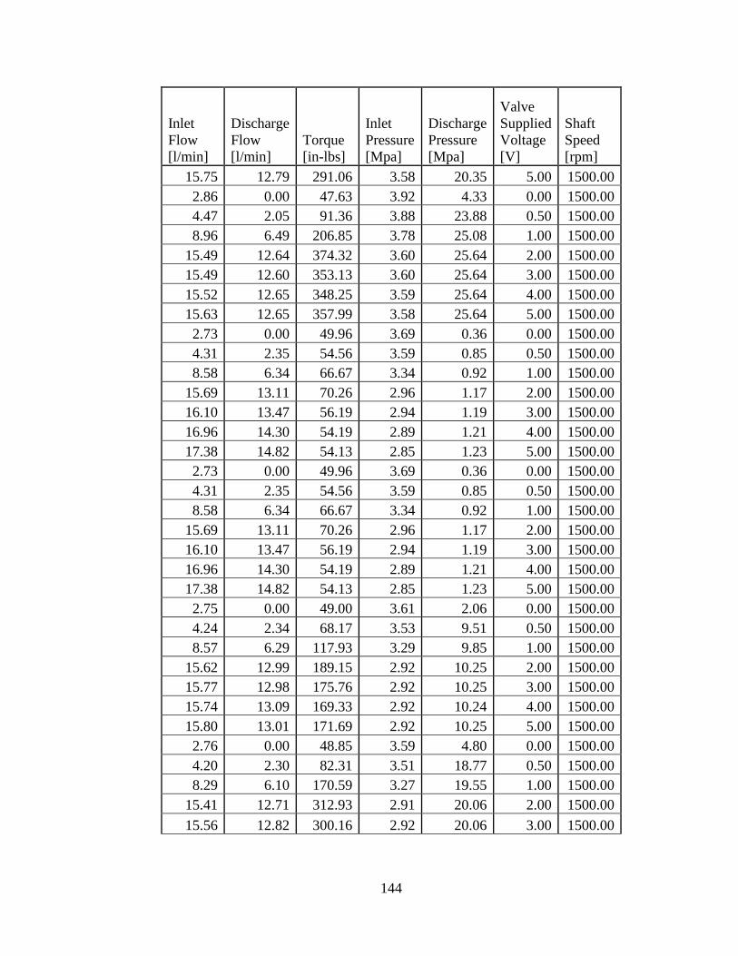
144
Inlet
Flow
[l/min]
Discharge
Flow
[l/min]
Torque
[in-lbs]
Inlet
Pressure
[Mpa]
Discharge
Pressure
[Mpa]
Valve
Supplied
Voltage
[V]
Shaft
Speed
[rpm]
15.75 12.79 291.06 3.58 20.35 5.00 1500.00
2.86 0.00 47.63 3.92 4.33 0.00 1500.00
4.47 2.05 91.36 3.88 23.88 0.50 1500.00
8.96 6.49 206.85 3.78 25.08 1.00 1500.00
15.49 12.64 374.32 3.60 25.64 2.00 1500.00
15.49 12.60 353.13 3.60 25.64 3.00 1500.00
15.52 12.65 348.25 3.59 25.64 4.00 1500.00
15.63 12.65 357.99 3.58 25.64 5.00 1500.00
2.73 0.00 49.96 3.69 0.36 0.00 1500.00
4.31 2.35 54.56 3.59 0.85 0.50 1500.00
8.58 6.34 66.67 3.34 0.92 1.00 1500.00
15.69 13.11 70.26 2.96 1.17 2.00 1500.00
16.10 13.47 56.19 2.94 1.19 3.00 1500.00
16.96 14.30 54.19 2.89 1.21 4.00 1500.00
17.38 14.82 54.13 2.85 1.23 5.00 1500.00
2.73 0.00 49.96 3.69 0.36 0.00 1500.00
4.31 2.35 54.56 3.59 0.85 0.50 1500.00
8.58 6.34 66.67 3.34 0.92 1.00 1500.00
15.69 13.11 70.26 2.96 1.17 2.00 1500.00
16.10 13.47 56.19 2.94 1.19 3.00 1500.00
16.96 14.30 54.19 2.89 1.21 4.00 1500.00
17.38 14.82 54.13 2.85 1.23 5.00 1500.00
2.75 0.00 49.00 3.61 2.06 0.00 1500.00
4.24 2.34 68.17 3.53 9.51 0.50 1500.00
8.57 6.29 117.93 3.29 9.85 1.00 1500.00
15.62 12.99 189.15 2.92 10.25 2.00 1500.00
15.77 12.98 175.76 2.92 10.25 3.00 1500.00
15.74 13.09 169.33 2.92 10.24 4.00 1500.00
15.80 13.01 171.69 2.92 10.25 5.00 1500.00
2.76 0.00 48.85 3.59 4.80 0.00 1500.00
4.20 2.30 82.31 3.51 18.77 0.50 1500.00
8.29 6.10 170.59 3.27 19.55 1.00 1500.00
15.41 12.71 312.93 2.91 20.06 2.00 1500.00
15.56 12.82 300.16 2.92 20.06 3.00 1500.00
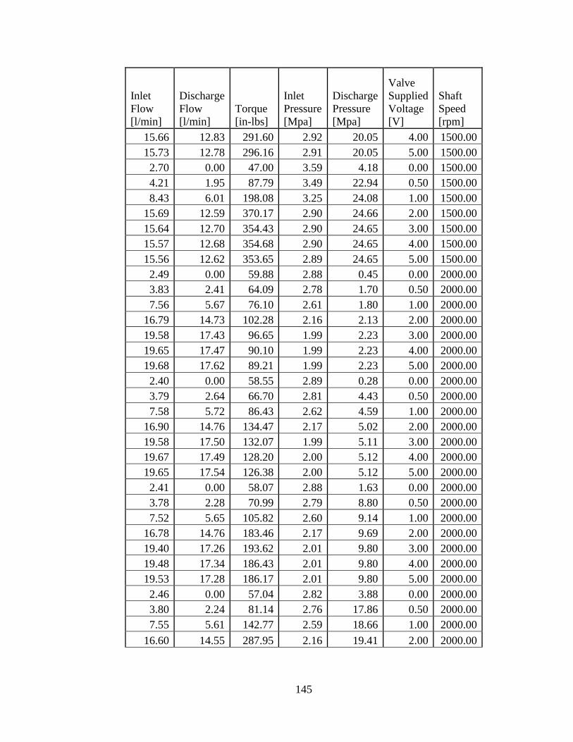
145
Inlet
Flow
[l/min]
Discharge
Flow
[l/min]
Torque
[in-lbs]
Inlet
Pressure
[Mpa]
Discharge
Pressure
[Mpa]
Valve
Supplied
Voltage
[V]
Shaft
Speed
[rpm]
15.66 12.83 291.60 2.92 20.05 4.00 1500.00
15.73 12.78 296.16 2.91 20.05 5.00 1500.00
2.70 0.00 47.00 3.59 4.18 0.00 1500.00
4.21 1.95 87.79 3.49 22.94 0.50 1500.00
8.43 6.01 198.08 3.25 24.08 1.00 1500.00
15.69 12.59 370.17 2.90 24.66 2.00 1500.00
15.64 12.70 354.43 2.90 24.65 3.00 1500.00
15.57 12.68 354.68 2.90 24.65 4.00 1500.00
15.56 12.62 353.65 2.89 24.65 5.00 1500.00
2.49 0.00 59.88 2.88 0.45 0.00 2000.00
3.83 2.41 64.09 2.78 1.70 0.50 2000.00
7.56 5.67 76.10 2.61 1.80 1.00 2000.00
16.79 14.73 102.28 2.16 2.13 2.00 2000.00
19.58 17.43 96.65 1.99 2.23 3.00 2000.00
19.65 17.47 90.10 1.99 2.23 4.00 2000.00
19.68 17.62 89.21 1.99 2.23 5.00 2000.00
2.40 0.00 58.55 2.89 0.28 0.00 2000.00
3.79 2.64 66.70 2.81 4.43 0.50 2000.00
7.58 5.72 86.43 2.62 4.59 1.00 2000.00
16.90 14.76 134.47 2.17 5.02 2.00 2000.00
19.58 17.50 132.07 1.99 5.11 3.00 2000.00
19.67 17.49 128.20 2.00 5.12 4.00 2000.00
19.65 17.54 126.38 2.00 5.12 5.00 2000.00
2.41 0.00 58.07 2.88 1.63 0.00 2000.00
3.78 2.28 70.99 2.79 8.80 0.50 2000.00
7.52 5.65 105.82 2.60 9.14 1.00 2000.00
16.78 14.76 183.46 2.17 9.69 2.00 2000.00
19.40 17.26 193.62 2.01 9.80 3.00 2000.00
19.48 17.34 186.43 2.01 9.80 4.00 2000.00
19.53 17.28 186.17 2.01 9.80 5.00 2000.00
2.46 0.00 57.04 2.82 3.88 0.00 2000.00
3.80 2.24 81.14 2.76 17.86 0.50 2000.00
7.55 5.61 142.77 2.59 18.66 1.00 2000.00
16.60 14.55 287.95 2.16 19.41 2.00 2000.00

146
Inlet
Flow
[l/min]
Discharge
Flow
[l/min]
Torque
[in-lbs]
Inlet
Pressure
[Mpa]
Discharge
Pressure
[Mpa]
Valve
Supplied
Voltage
[V]
Shaft
Speed
[rpm]
18.95 16.91 317.50 2.02 19.59 3.00 2000.00
19.04 16.87 309.36 2.02 19.58 4.00 2000.00
19.12 16.85 305.92 2.02 19.59 5.00 2000.00
2.54 0.00 55.72 2.74 3.46 0.00 2000.00
3.87 2.35 84.53 2.70 22.41 0.50 2000.00
7.47 5.52 158.61 2.56 23.61 1.00 2000.00
16.39 14.33 337.01 2.13 24.44 2.00 2000.00
18.97 16.64 380.46 1.99 24.64 3.00 2000.00
19.00 16.67 374.60 2.00 24.63 4.00 2000.00
19.11 16.76 358.47 2.00 24.64 5.00 2000.00
2.00 0.00 60.73 1.81 0.39 0.00 2500.00
3.02 2.04 63.61 1.75 1.69 0.50 2500.00
5.95 4.38 71.08 1.64 1.80 1.00 2500.00
12.94 11.21 91.98 1.33 2.00 2.00 2500.00
19.20 17.38 107.15 1.04 2.22 3.00 2500.00
22.22 20.64 112.10 0.90 2.32 4.00 2500.00
23.18 21.44 111.57 0.85 2.36 5.00 2500.00
2.02 0.00 60.53 1.80 1.56 0.00 2500.00
3.06 1.83 64.65 1.75 4.20 0.50 2500.00
5.94 4.39 78.39 1.63 4.35 1.00 2500.00
12.92 11.23 112.17 1.33 4.60 2.00 2500.00
19.04 17.32 134.13 1.04 4.86 3.00 2500.00
22.39 20.60 147.24 0.89 4.99 4.00 2500.00
23.23 21.39 144.30 0.86 5.03 5.00 2500.00
2.05 0.00 71.67 1.88 0.19 0.00 2500.00
3.10 1.85 83.23 1.82 9.42 0.50 2500.00
6.04 4.32 107.78 1.67 9.86 1.00 2500.00
12.86 11.40 164.69 1.35 10.23 2.00 2500.00
18.18 17.11 211.42 1.05 10.56 3.00 2500.00
21.52 20.39 232.83 0.89 10.73 4.00 2500.00
22.24 21.14 234.17 0.85 10.78 5.00 2500.00
1.98 0.00 65.68 1.81 4.39 0.00 2500.00
3.04 1.55 83.19 1.77 18.04 0.50 2500.00
5.95 4.28 122.93 1.65 18.83 1.00 2500.00

147
Inlet
Flow
[l/min]
Discharge
Flow
[l/min]
Torque
[in-lbs]
Inlet
Pressure
[Mpa]
Discharge
Pressure
[Mpa]
Valve
Supplied
Voltage
[V]
Shaft
Speed
[rpm]
12.89 11.22 221.78 1.34 19.39 2.00 2500.00
18.76 16.97 301.77 1.05 19.83 3.00 2500.00
22.01 20.29 338.96 0.90 20.09 4.00 2500.00
22.67 20.90 349.69 0.87 20.14 5.00 2500.00
1.97 0.00 62.80 1.78 7.39 0.00 2500.00
3.08 1.97 85.27 1.75 23.92 0.50 2500.00
5.99 4.24 137.65 1.64 25.02 1.00 2500.00
12.73 11.04 256.80 1.33 25.67 2.00 2500.00
18.54 16.71 362.62 1.05 26.17 3.00 2500.00
21.84 20.01 413.07 0.90 26.46 4.00 2500.00
22.32 20.50 422.39 0.88 26.48 5.00 2500.00

148
VITA
Julie Wisch was born in Jefferson City, Missouri in 1989 to Kevin and Karen
Wisch. She has one brother, Stephen Wisch. She attended Immaculate Conception for
kindergarten through eighth grade, and then attended Helias High School, where she
graduated in 2007. Upon graduation, she matriculated to the University of Iowa, where
she briefly studied biomedical engineering before determining that mechanical
engineering required significantly fewer chemistry classes. She earned a Bachelor of
Science degree in Mechanical Engineering in 2011 from the University of Iowa.
Following her graduation from the University of Iowa, Julie joined Accenture in
Chicago, Illinois. From June 2011 to January 2013, Julie was staffed on projects at
Caterpillar, BP, and Exelon. She was a consultant for a year and a half, and is still
incapable of explaining exactly what it is that a consultant does.
Julie completed her doctoral work at the University of Missouri in hydraulic
systems under the guidance of Dr. Noah Manring. She greatly enjoyed the opportunity to
work on an industry-driven project, and is pleased to have had the chance to collaborate
with engineers at Caterpillar. Outside of her graduate work, she served as the assistant
softball coach at Tolton Catholic High School from 2013 - 2015, and is deeply grateful to
the Tolton community for having a place to play and do something entirely unrelated to
her academic life. She defended her dissertation in April of 2016, and plans to move to
Fayetteville, Arkansas following graduation to work in the Fayetteville Public School
District and launch a STEM program at the Agee-Lierly Life Preparation Services
Center.