Open Journal of Civil Engineering, 2015, 5, 359‐371 Published Online December 2015 in SciRes. http://www.scirp.org/journal/ojce http://dx.doi.org/10.4236/ojce.2015.54036     

How to cite this paper: Dua, A., Clobes, M., Höbbel, T. and Matsagar, V. (2015) Dynamic Analysis of Overhead Transmission Lines under Turbulent Wind Loading. Open Journal of Civil Engineering, 5, 359‐371.   http://dx.doi.org/10.4236/ojce.2015.54036   

DynamicAnalysisofOverheadTransmissionLinesunderTurbulentWindLoading

AlokDua1,MathiasClobes2,ThomasHöbbel2,VasantMatsagar11Department of Civil Engineering, Indian Institute of Technology (IIT), Delhi, India 2Institut für Stahlbau, Technische Universität Carolo‐Wilhelmina, Braunschweig, Germany 

    Received 23 September 2015; accepted 21 November 2015; published 24 November 2015 

Copyright © 2015 by authors and Scientific Research Publishing Inc. This work is licensed under the Creative Commons Attribution International License (CC BY). http://creativecommons.org/licenses/by/4.0/ 

  

Abstract

Transmissiontower‐linesystemsaredesignedusingstatic loadsspecified invariouscodes.ThispapercomparesthedynamicresponseofatesttransmissionlinewiththeresponseduetostaticloadsgivenbyEurocode.FiniteelementdesignsoftwareSAP2000wasusedtomodelthetowersand lines.Non‐lineardynamicanalysis including the largedisplacementeffectswascarriedout.Macroscopicaspectsofwindcoherencealongelement lengthand integrationtimestepwere in‐vestigated.Anapproachispresentedtocomparetheprobabilisticdynamicresponsedueto7dif‐ferentstochasticallysimulatedwind fieldswith theresponseaccording toEN‐50341.Thedevel‐opedmodelwillbeusedtostudytheresponserecordedonatestlineduetotheactualwindspeedtimehistoryrecorded. Itwas found thatstatic load fromENoverestimated thestrengthofcon‐ductorcables.Theresponseofcoupledsystemconsideringtowersandcableswasfoundtobedif‐ferentfromresponseofonlycableswithfixedsupports.

Keywords

DynamicAnalysis,FiniteElementMethod,SAP2000,TransmissionTowers,TransmissionLines

1.Introduction

Collapse of transmission tower-line systems is not a well understood phenomenon. These systems are subjected to various loads like wind, snow, icing and earthquake. Comparatively, wind loads are more complex for these structures due to high geometric non-linearity of cables and randomness of wind turbulence. This thesis is aimed at understanding the dynamic behavior of transmission tower-line systems under fluctuating wind loads. Present code recommendations are based on static loading. In this paper, [1] was considered for comparison of results. EN-50341 gives wind pressure including 2 second gusts with peak wind velocities, for conductors, insulators

A.Duaetal.

360

and towers. In the present design practice, towers and conductors are considered separately ignoring the cou-pling effect and static loads are applied individually.

Coupled transmission tower-line systems are highly complex in their behavior due to the interaction between non-linear conductors and stiff towers which results in closely spaced frequencies. [2] studied these systems considering the geometric non-linearity and aerodynamic damping; however the work was not in 3 dimensions. [3] presented linear response in a coupled system using a 3D finite element model. [4] recently showed that the design codes overestimate the strength of transmission towers. They brought out that a 3D finite element analy-sis is more accurate compared to linear analysis. Until now, not many researchers have studied the coupling ef-fect on response of cables using non-linear dynamic analysis. Previous studies were linear and without the ef-fects of large displacements. Secondly, the response of such systems is usually assumed as Gaussian for con-venience in calculating the extreme response.

A 3D non-linear analysis including the large displacements was carried out to study the dynamic response of conductors. Effects of parameters like coherence along element length and integration time step were considered. The response of cables and insulators was found to be non-Gaussian. Methods lately published for calculating extreme values of a non-Gaussian process were used. These extreme values were then compared to the response due to wind pressure recommended in EN-50341. The chosen transmission line is in Rostock, Germany. It has 2 end towers and 2 suspension towers. Each of the 3 spans is about 400 m. A 3D finite element model of a real transmission line was modeled in finite element software SAP2000. Two models were studied: only conductors and conductors coupled with towers. The results were compared to show the importance of conductor-tower in-teraction.

2.DetailsoftheModel

2.1.ChosenTestLine

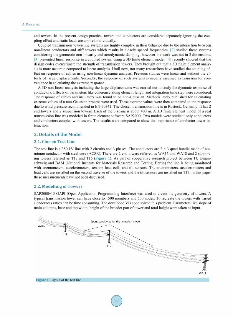
The test line is a 380 kV line with 2 circuits and 3 phases. The conductors are 2 × 3 quad bundle made of alu-minum conductor with steel core (ACSR). There are 2 end towers referred as WA15 and WA18 and 2 support-ing towers referred as T17 and T16 (Figure 1). As part of cooperative research project between TU Braun-schweig and BAM (National Institute for Materials Research and Testing, Berlin) the line is being monitored with anemometers, accelerometers, tension load cells and tilt sensors. The anemometers, accelerometers and load cells are installed on the second traverse of the towers and the tilt sensors are installed on T17. In this paper these measurements have not been discussed.

2.2.ModellingofTowers

SAP2000v15 OAPI (Open Application Programming Interface) was used to create the geometry of towers. A typical transmission tower can have close to 1500 members and 500 nodes. To recreate the towers with varied slenderness ratios can be time consuming. The developed VB code solved this problem. Parameters like slope of main columns, base and top width, height of the broader part of tower and total height were taken as input.

Figure 1. Layout of the test line.

A.Duaetal.

361

In past, [5]- [10] have brought out the importance of connections in transmission towers. Only geometric and material non-linear analysis can fully depict the behavior. In this study, the towers were modeled as a beam-truss model. Rigid connections (with two or more bolts) were modeled using beam elements. Flexible connections (single bolt) were modeled using truss elements with moment released about appropriate direction. This is an approximation and ideally flexible connections should have some stiffness. The eccentricity in the connections and the load application point has been ignored. European norms recommend these structures to be in elastic range during service life. Hence, material non-linearity has not been considered in the model.

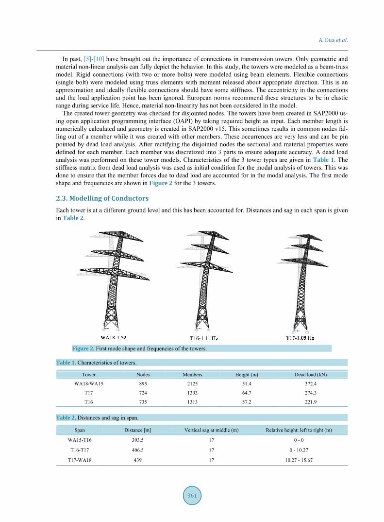
The created tower geometry was checked for disjointed nodes. The towers have been created in SAP2000 us-ing open application programming interface (OAPI) by taking required height as input. Each member length is numerically calculated and geometry is created in SAP2000 v15. This sometimes results in common nodes fal-ling out of a member while it was created with other members. These occurrences are very less and can be pin pointed by dead load analysis. After rectifying the disjointed nodes the sectional and material properties were defined for each member. Each member was discretized into 3 parts to ensure adequate accuracy. A dead load analysis was performed on these tower models. Characteristics of the 3 tower types are given in Table 1. The stiffness matrix from dead load analysis was used as initial condition for the modal analysis of towers. This was done to ensure that the member forces due to dead load are accounted for in the modal analysis. The first mode shape and frequencies are shown in Figure 2 for the 3 towers.

2.3.ModellingofConductors

Each tower is at a different ground level and this has been accounted for. Distances and sag in each span is given in Table 2.

Figure 2. First mode shape and frequencies of the towers.

Table 1. Characteristics of towers.

Tower Nodes Members Height (m) Dead load (kN)

WA18/WA15 895 2125 51.4 372.4

T17 724 1393 64.7 274.3

T16 735 1313 57.2 221.9

Table 2. Distances and sag in span.

Span Distance [m] Vertical sag at middle (m) Relative height: left to right (m)

WA15-T16 393.5 17 0 - 0

T16-T17 406.5 17 0 - 10.27

T17-WA18 439 17 10.27 - 15.67

A.Duaetal.

362

The conductors were modeled as tension-only linear elastic material. The non-linearity of these flexible cables was taken into account for dynamic analysis. Quad bundle of conductors was assumed as one conductor with 4 times cross sectional area. In this study, each conductor was divided into 20 parts for application of wind load time histories. The sectional and material properties for conductors are given in Table 3.

2.4.DampinginConductors

The sectional and material properties for towers, insulator strings and conductors are as per the technical draw-ings. Realistic modeling of aerodynamic damping is very complex for such systems. Aerodynamic damping af-fects the conductors in a varied way. Aerodynamic damping is an aeroelastic phenomenon and opposes the ac-tion of cables depending on the direction of motion. This cannot be modeled in SAP2000v15 however a satis-factory model has been recently presented by [11] using commercial software ADINA. For this study the aero-dynamic damping was incorporated as viscous damping. An equivalent viscous material damping ratio of 2% is sufficient to model the aerodynamic damping effects on the conductors [3]; [8]. Apart from aerodynamic damp-ing in conductors, 0.5% damping ratio was used to account for structural damping due to steel material, connec-tions and the foundation.

2.5.InsulatorStrings

In most of the numerical research works, either the insulator strings have not been modeled or have been as-sumed to be a beam element while towers have been neglected. [12] have discussed about the importance of in-sulator string in overhead transmission line under wind load. As per their study, the non-rigid insulator strings have to be modeled as per the real material, sectional and boundary properties. It is not accurate to assume the insulator strings as rigid beam elements. In this study, the insulator strings were modeled as cable elements to account for the local slackening effects in the flexible insulator strings. However, a better model as discussed by [12] may be used to get more accurate results for failure criteria of insulators.

2.6.SimplificationofTowers

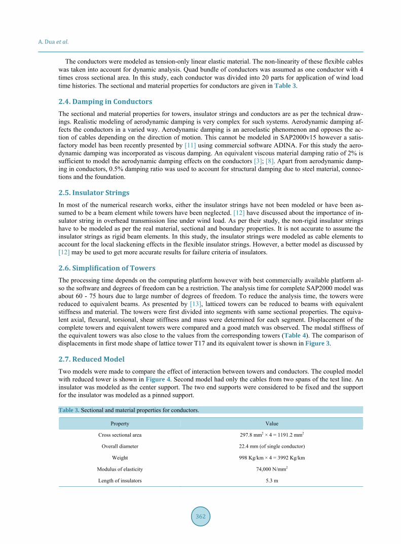
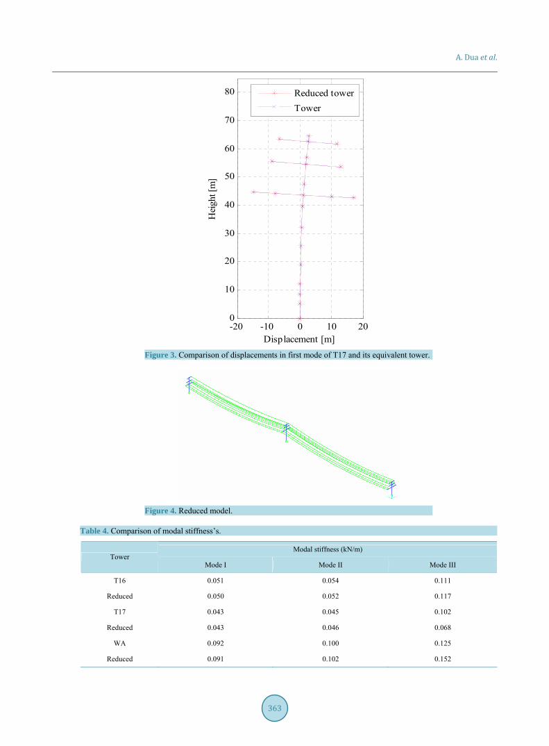
The processing time depends on the computing platform however with best commercially available platform al-so the software and degrees of freedom can be a restriction. The analysis time for complete SAP2000 model was about 60 - 75 hours due to large number of degrees of freedom. To reduce the analysis time, the towers were reduced to equivalent beams. As presented by [13], latticed towers can be reduced to beams with equivalent stiffness and material. The towers were first divided into segments with same sectional properties. The equiva-lent axial, flexural, torsional, shear stiffness and mass were determined for each segment. Displacement of the complete towers and equivalent towers were compared and a good match was observed. The modal stiffness of the equivalent towers was also close to the values from the corresponding towers (Table 4). The comparison of displacements in first mode shape of lattice tower T17 and its equivalent tower is shown in Figure 3.

2.7.ReducedModel

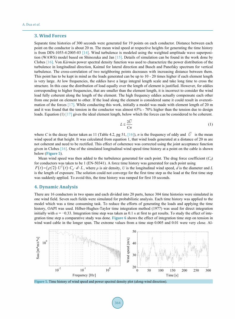
Two models were made to compare the effect of interaction between towers and conductors. The coupled model with reduced tower is shown in Figure 4. Second model had only the cables from two spans of the test line. An insulator was modeled as the center support. The two end supports were considered to be fixed and the support for the insulator was modeled as a pinned support.

Table 3. Sectional and material properties for conductors.

Property Value

Cross sectional area 297.8 mm2 × 4 = 1191.2 mm2

Overall diameter 22.4 mm (of single conductor)

Weight 998 Kg/km × 4 = 3992 Kg/km

Modulus of elasticity 74,000 N/mm2

Length of insulators 5.3 m

A.Duaetal.

363

-20 -10 0 10 200

10

20

30

40

50

60

70

80

Displacement [m]

Hei

ght [

m]

Reduced tower

Tower

Figure 3. Comparison of displacements in first mode of T17 and its equivalent tower.

Figure 4. Reduced model.

Table 4. Comparison of modal stiffness’s.

Modal stiffness (kN/m) Tower

Mode I Mode II Mode III

T16 0.051 0.054 0.111

Reduced 0.050 0.052 0.117

T17 0.043 0.045 0.102

Reduced 0.043 0.046 0.068

WA 0.092 0.100 0.125

Reduced 0.091 0.102 0.152

A.Duaetal.

364

3.WindForces

Separate time histories of 300 seconds were generated for 19 points on each conductor. Distance between each point on the conductor is about 20 m. The mean wind speed at respective heights for generating the time history is from DIN-1055-4:2005-03 [14]. Wind turbulence is modeled using the weighted amplitude wave superposi-tion (WAWS) model based on Shinozuka and Jan [15]. Details of simulation can be found in the work done by Clobes [16]. Von Kármán power spectral density function was used to characterize the power distribution of the turbulence in longitudinal direction, Kaimal for lateral direction and Busch and Panofsky spectrum for vertical turbulence. The cross-correlation of two neighboring points decreases with increasing distance between them. This point has to be kept in mind as the loads generated can be up to 10 - 20 times higher if each element length is very large. At low frequencies, the eddies have a large integral length scale and take long time to cross the structure. In this case the distribution of load equally over the length of element is justified. However, for eddies corresponding to higher frequencies, that are smaller than the element length, it is incorrect to consider the wind load fully coherent along the length of the element. The high frequency eddies actually compensate each other from one point on element to other. If the load along the element is considered same it could result in overesti-mation of the forces [17]. While conducting this work, initially a model was made with element length of 20 m and it was found that the tension in the conductor was almost 65% - 70% higher than the tension due to design loads. Equation (1) [17] gives the ideal element length, below which the forces can be considered to be coherent.

2UL

Cn (1)

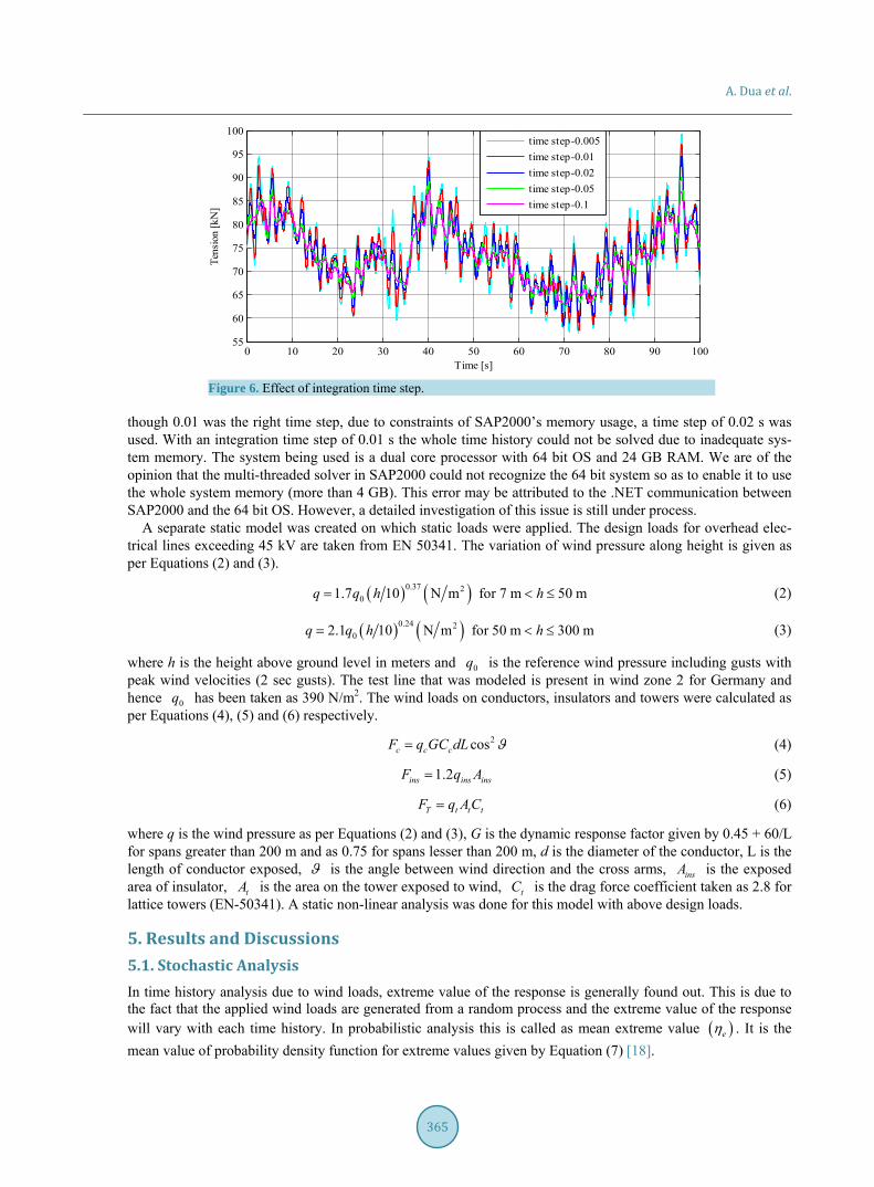
where C is the decay factor taken as 11 (Table 4.2, pg 51, [16]), n is the frequency of eddy and U is the mean wind speed at that height. It was calculated from equation 1, that wind loads generated at a distance of 20 m are not coherent and need to be rectified. This effect of coherence was corrected using the joint acceptance function given in Clobes [16]. One of the simulated longitudinal wind speed time history at a point on the cable is shown below (Figure 5).

Mean wind speed was then added to the turbulence generated for each point. The drag force coefficient (Cd) for conductors was taken to be 1 (EN-50341). A force time history was generated for each point using 22 dF t U t C d L , where ρ is air density, U is the longitudinal wind speed, d is the diameter and L

is the length of exposure. The solution could not converge for the first time step as the load at the first time step was suddenly applied. To avoid this, the time history was ramped for first 10 seconds.

4.DynamicAnalysis

There are 16 conductors in two spans and each divided into 20 parts, hence 304 time histories were simulated in one wind field. Seven such fields were simulated for probabilistic analysis. Each time history was applied to the model which was a time consuming task. To reduce the efforts of generating the loads and applying the time history, OAPI was used. Hilber-Hughes-Taylor time integration method (1977) was used for direct integration initially with α = −0.33. Integration time step was taken as 0.1 s at first to get results. To study the effect of inte-gration time step a comparative study was done. Figure 6 shows the effect of integration time step on tension in wind ward cable in the longer span. The extreme values from a time step 0.005 and 0.01 were very close. Al-

10-2

10-1

100

100

Frequency [Hz]

Suu

[m

*m/s

*s]

0 50 100 150 200 250 30020

30

40

50

Time [s]

Win

d sp

eed

[m/s

]

Figure 5. Time history of wind speed and power spectral density plot (along-wind direction).

A.Duaetal.

365

0 10 20 30 40 50 60 70 80 90 10055

60

65

70

75

80

85

90

95

100

Time [s]

Ten

sion

[kN

]

time step-0.005

time step-0.01

time step-0.02

time step-0.05

time step-0.1

Figure 6. Effect of integration time step.

though 0.01 was the right time step, due to constraints of SAP2000’s memory usage, a time step of 0.02 s was used. With an integration time step of 0.01 s the whole time history could not be solved due to inadequate sys-tem memory. The system being used is a dual core processor with 64 bit OS and 24 GB RAM. We are of the opinion that the multi-threaded solver in SAP2000 could not recognize the 64 bit system so as to enable it to use the whole system memory (more than 4 GB). This error may be attributed to the .NET communication between SAP2000 and the 64 bit OS. However, a detailed investigation of this issue is still under process.

A separate static model was created on which static loads were applied. The design loads for overhead elec-trical lines exceeding 45 kV are taken from EN 50341. The variation of wind pressure along height is given as per Equations (2) and (3).

0.37 201.7 10 N m for 7 m 50 mq q h h (2)

0.24 202.1 10 N m for 50 m 300 mq q h h (3)

where h is the height above ground level in meters and 0q is the reference wind pressure including gusts with peak wind velocities (2 sec gusts). The test line that was modeled is present in wind zone 2 for Germany and hence 0q has been taken as 390 N/m2. The wind loads on conductors, insulators and towers were calculated as per Equations (4), (5) and (6) respectively.

2cosc c cF q GC dL (4)

1.2ins ins insF q A (5)

T t t tF q A C (6)

where q is the wind pressure as per Equations (2) and (3), G is the dynamic response factor given by 0.45 + 60/L for spans greater than 200 m and as 0.75 for spans lesser than 200 m, d is the diameter of the conductor, L is the length of conductor exposed, is the angle between wind direction and the cross arms, insA is the exposed area of insulator, tA is the area on the tower exposed to wind, tC is the drag force coefficient taken as 2.8 for lattice towers (EN-50341). A static non-linear analysis was done for this model with above design loads.

5.ResultsandDiscussions

5.1.StochasticAnalysis

In time history analysis due to wind loads, extreme value of the response is generally found out. This is due to the fact that the applied wind loads are generated from a random process and the extreme value of the response will vary with each time history. In probabilistic analysis this is called as mean extreme value e . It is the

mean value of probability density function for extreme values given by Equation (7) [18].

A.Duaetal.

366

2exp exp 2e eP T (7)

where ν is the mean frequency of occurrence of zero crossings with positive slopes only and is given by Equa-tion (8).

1 2

2 0

1

2πm m

and

nn xm S

(8)

here xS is the power spectral density function of the random process. It has been shown by [19] that the mean extreme value can be given with an approximate relation (Equation

(9)) derived from Equation (7).

1 2 1 22 ln 2 lne T T (9)

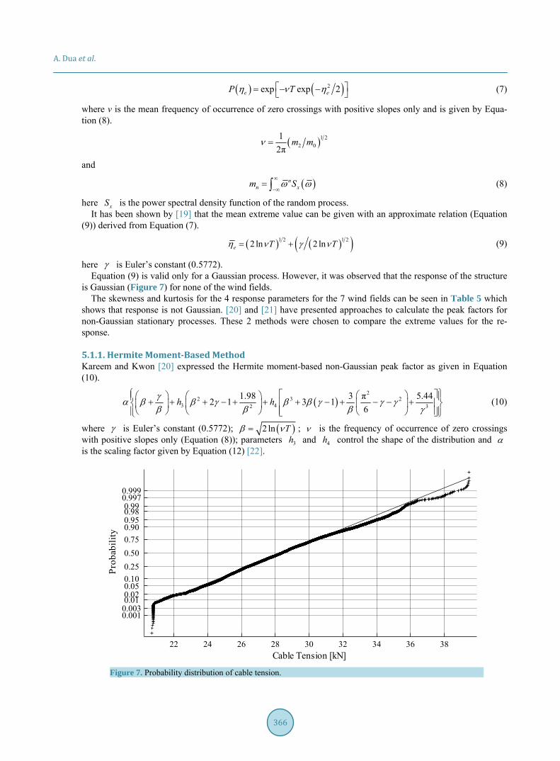
here is Euler’s constant (0.5772). Equation (9) is valid only for a Gaussian process. However, it was observed that the response of the structure

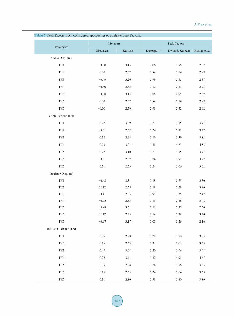
is Gaussian (Figure 7) for none of the wind fields. The skewness and kurtosis for the 4 response parameters for the 7 wind fields can be seen in Table 5 which

shows that response is not Gaussian. [20] and [21] have presented approaches to calculate the peak factors for non-Gaussian stationary processes. These 2 methods were chosen to compare the extreme values for the re-sponse.

5.1.1.HermiteMoment‐BasedMethodKareem and Kwon [20] expressed the Hermite moment-based non-Gaussian peak factor as given in Equation (10).

2

2 3 23 42 3

1.98 3 π 5.442 1 3 1

6h h

(10)

where is Euler’s constant (0.5772); 2 ln T ; is the frequency of occurrence of zero crossings with positive slopes only (Equation (8)); parameters 3h and 4h control the shape of the distribution and is the scaling factor given by Equation (12) [22].

22 24 26 28 30 32 34 36 38

0.0010.0030.01 0.02 0.05 0.10

0.25

0.50

0.75

0.90 0.95 0.98 0.99

0.9970.999

Cable Tension [kN]

Pro

babi

lity

Figure 7. Probability distribution of cable tension.

A.Duaetal.

367

Table 5. Peak factors from considered approaches to evaluate peak factors.

Moments Peak Factors Parameter

Skewness Kurtosis Davenport Kwon & Kareem Huang et al.

Cable Disp. (m)

TH1 −0.30 3.13 3.06 2.75 2.67

TH2 0.07 2.57 2.89 2.59 2.98

TH3 −0.49 3.26 2.99 2.55 2.37

TH4 −0.30 2.65 3.12 2.21 2.73

TH5 −0.30 3.13 3.06 2.75 2.67

TH6 0.07 2.57 2.89 2.59 2.98

TH7 −0.001 2.59 2.91 2.52 2.92

Cable Tension (kN)

TH1 0.27 3.09 3.23 3.75 3.71

TH2 −0.01 2.62 3.24 2.71 3.27

TH3 0.38 2.64 3.19 3.39 3.82

TH4 0.70 3.24 3.31 4.63 4.53

TH5 0.27 3.10 3.23 3.75 3.71

TH6 −0.01 2.62 3.24 2.71 3.27

TH7 0.21 2.59 3.24 3.06 3.62

Insulator Disp. (m)

TH1 −0.48 3.31 3.18 2.75 2.50

TH2 0.112 2.35 3.19 2.28 3.40

TH3 −0.41 2.93 2.98 2.35 2.47

TH4 −0.05 2.55 3.11 2.48 3.08

TH5 −0.48 3.31 3.18 2.75 2.50

TH6 0.112 2.35 3.19 2.28 3.40

TH7 −0.67 3.17 3.05 2.26 2.16

Insulator Tension (kN)

TH1 0.35 2.98 3.24 3.78 3.85

TH2 0.16 2.63 3.24 3.04 3.55

TH3 0.48 3.04 3.20 3.96 3.98

TH4 0.72 3.41 3.37 4.91 4.67

TH5 0.35 2.98 3.24 3.78 3.85

TH6 0.16 2.63 3.24 3.04 3.55

TH7 0.31 2.80 3.31 3.60 3.89

A.Duaetal.

368

2 23 4

33

4

44

1

1 2 6

4 2 1 1.5 3

1 1.5 3 1

18

h h

h

h

(12)

5.1.2.SkewnessDependentPeakFactor [21] studied the peak factor of mild non-Gaussian process. They recommended a simplified empirical formula for non-Gaussian peak factor dependent only on the skewness but effect of mild softening has been empirically calibrated (Equation (12)).

2 2 23ln 2 2 16skewg

(13)

where the variables have the same meaning as in Equation (10).

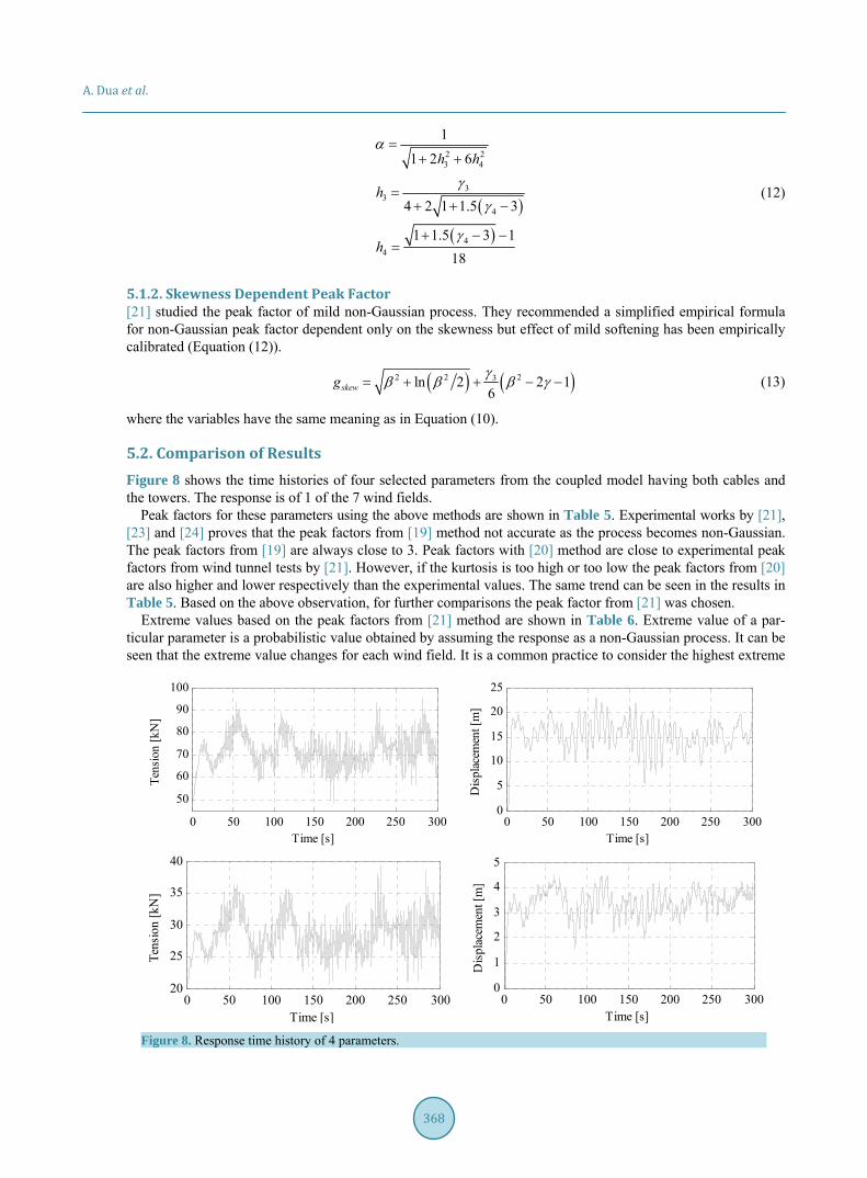
5.2.ComparisonofResults

Figure 8 shows the time histories of four selected parameters from the coupled model having both cables and the towers. The response is of 1 of the 7 wind fields.

Peak factors for these parameters using the above methods are shown in Table 5. Experimental works by [21], [23] and [24] proves that the peak factors from [19] method not accurate as the process becomes non-Gaussian. The peak factors from [19] are always close to 3. Peak factors with [20] method are close to experimental peak factors from wind tunnel tests by [21]. However, if the kurtosis is too high or too low the peak factors from [20] are also higher and lower respectively than the experimental values. The same trend can be seen in the results in Table 5. Based on the above observation, for further comparisons the peak factor from [21] was chosen.

Extreme values based on the peak factors from [21] method are shown in Table 6. Extreme value of a par-ticular parameter is a probabilistic value obtained by assuming the response as a non-Gaussian process. It can be seen that the extreme value changes for each wind field. It is a common practice to consider the highest extreme

0 50 100 150 200 250 300

50

60

70

80

90

100

Time [s]

Ten

sion

[kN

]

0 50 100 150 200 250 300

0

5

10

15

20

25

Time [s]

Dis

plac

emen

t [m

]

0 50 100 150 200 250 30020

25

30

35

40

Time [s]

Ten

sion

[kN

]

0 50 100 150 200 250 3000

1

2

3

4

5

Time [s]

Dis

plac

emen

t [m

]

Figure 8. Response time history of 4 parameters.

A.Duaetal.

369

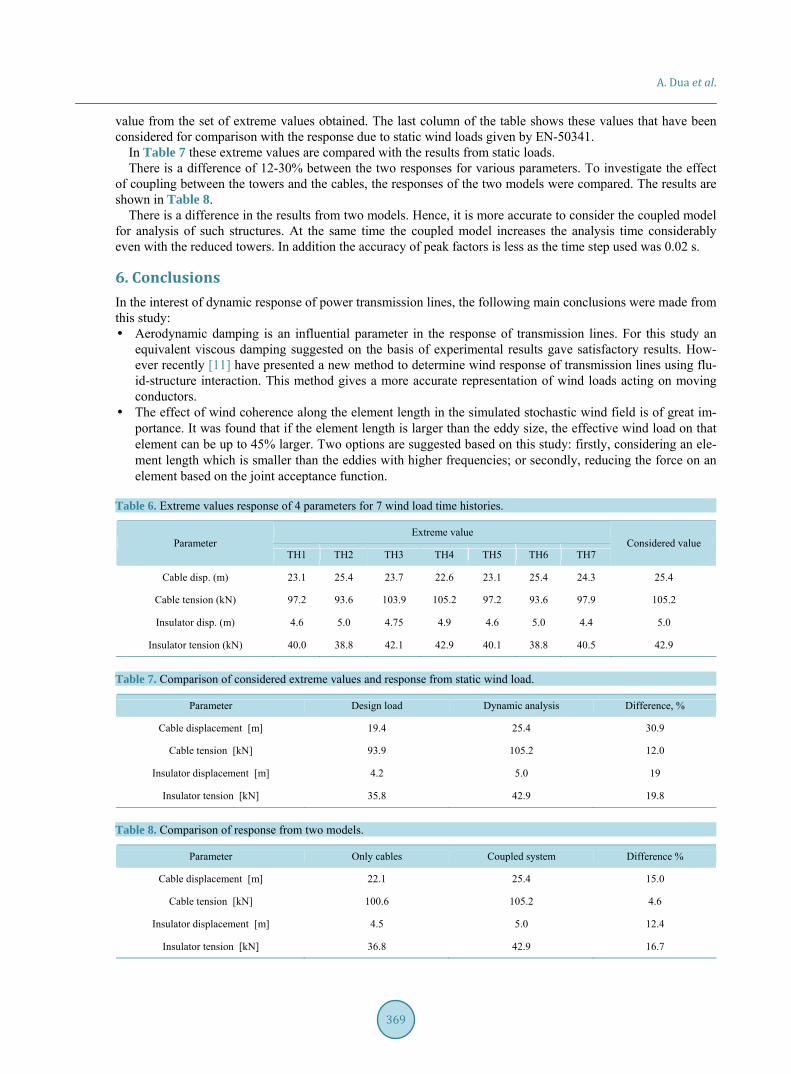
value from the set of extreme values obtained. The last column of the table shows these values that have been considered for comparison with the response due to static wind loads given by EN-50341.

In Table 7 these extreme values are compared with the results from static loads. There is a difference of 12-30% between the two responses for various parameters. To investigate the effect

of coupling between the towers and the cables, the responses of the two models were compared. The results are shown in Table 8.

There is a difference in the results from two models. Hence, it is more accurate to consider the coupled model for analysis of such structures. At the same time the coupled model increases the analysis time considerably even with the reduced towers. In addition the accuracy of peak factors is less as the time step used was 0.02 s.

6.Conclusions

In the interest of dynamic response of power transmission lines, the following main conclusions were made from this study: Aerodynamic damping is an influential parameter in the response of transmission lines. For this study an

equivalent viscous damping suggested on the basis of experimental results gave satisfactory results. How-ever recently [11] have presented a new method to determine wind response of transmission lines using flu-id-structure interaction. This method gives a more accurate representation of wind loads acting on moving conductors.

The effect of wind coherence along the element length in the simulated stochastic wind field is of great im-portance. It was found that if the element length is larger than the eddy size, the effective wind load on that element can be up to 45% larger. Two options are suggested based on this study: firstly, considering an ele-ment length which is smaller than the eddies with higher frequencies; or secondly, reducing the force on an element based on the joint acceptance function.

Table 6. Extreme values response of 4 parameters for 7 wind load time histories.

Extreme value Parameter

TH1 TH2 TH3 TH4 TH5 TH6 TH7 Considered value

Cable disp. (m) 23.1 25.4 23.7 22.6 23.1 25.4 24.3 25.4

Cable tension (kN) 97.2 93.6 103.9 105.2 97.2 93.6 97.9 105.2

Insulator disp. (m) 4.6 5.0 4.75 4.9 4.6 5.0 4.4 5.0

Insulator tension (kN) 40.0 38.8 42.1 42.9 40.1 38.8 40.5 42.9

Table 7. Comparison of considered extreme values and response from static wind load.

Parameter Design load Dynamic analysis Difference, %

Cable displacement [m] 19.4 25.4 30.9

Cable tension [kN] 93.9 105.2 12.0

Insulator displacement [m] 4.2 5.0 19

Insulator tension [kN] 35.8 42.9 19.8

Table 8. Comparison of response from two models.

Parameter Only cables Coupled system Difference %

Cable displacement [m] 22.1 25.4 15.0

Cable tension [kN] 100.6 105.2 4.6

Insulator displacement [m] 4.5 5.0 12.4

Insulator tension [kN] 36.8 42.9 16.7

A.Duaetal.

370

Response of a transmission line to gust wind is non-Gaussian in nature. An appropriate method to calculate the peak factor for a non-Gaussian random process gave results that were higher than the davenport’s peak factors. A numerical verification of these peak factors can be envisaged as a future research task.

Static wind loads specified in EN-50341 overestimate the cable strength. Extreme values of 4 response pa-rameters were found to be greater than the static design response.

The response for a coupled model is different from the response when only the cables are considered. The results from the model with only the cables gave wrong estimations for the displacements of lines and insu-lators. The swing angle of insulators can be larger in coupled model thereby resulting in flashovers. To ac-count for the difference in displacement values, it is recommended to use an equivalent stiffness at supports, instead of the towers, in the model with only cables. This can reduce the analysis time to 3 - 4 hours and also satisfactorily account for the difference in the response as compared to the coupled model.

As a future scope for the project, it would be interesting to input the wind speed records from the test line and compare the numerical response with the recoded response. The insulator swing angle can be conven-iently calculated from the numerical model and the same parameter is being recorded at the test line.

References[1] European Committee for Standardisation (2010) DIN-EN-50341-3-4-VDE-0210-3, Overhead Electrical Lines Exceed-

ing AC 45 kV. Part I—General Requirements—Common Specifications. European Committee for Standardisation, Germany.

[2] Yasui, H., Marukawa, H., Momomura, Y. and Ohkuma, T. (1999) Analytical Study on Wind-Induced Vibration of Power Transmission Towers. Journal of Wind Engineering and Industrial Aerodynamics, 83, 431-441. http://dx.doi.org/10.1016/S0167-6105(99)00091-4

[3] Battista, R.C., Rodrigues, R.S. and Pfeil, M.S. (2003) Dynamic Behavior and Stability of Transmission Line Towers under Wind Forces. Journal of Wind Engineering and Industrial Aerodynamics, 91, 1051-1067. http://dx.doi.org/10.1016/S0167-6105(03)00052-7

[4] Rao, N.P., Légeron, F. and Prud’homme, S. (2012) Variation of Damping and Stiffness of Lattice Towers with Load Level. Journal of Constructional Steel Research, 71, 111-118. http://dx.doi.org/10.1016/j.jcsr.2011.10.018

[5] Robert, V. and Lemelin, D.R. (2002) Flexural Consideration in Steel Transmission Tower Design. In: Electrical Transmission in a New Age, ASCE, Omaha. http://dx.doi.org/10.1061/40642(253)11

[6] Albermani, F.G.A. and Kitipornchai, S. (2003) Numerical Simulation of Structural Behavior of Transmission Towers. Journal of Thin-Walled Structures, 41, 167-177. http://dx.doi.org/10.1016/S0263-8231(02)00085-X

[7] da Silva, J.G.S., da Vellasco, P.C.G., de Andrade, S.A.L. and de Oliveira, M.I.R. (2005) Structural Assessment of Current Steel Design Models for Transmission and Telecommunication Towers. Journal of Constructional Steel Re-search, 61, 1108-1134. http://dx.doi.org/10.1016/j.jcsr.2005.02.009

[8] McClure, G. and Lapointe, M. (2003) Modeling the Structural Dynamic Response of Overhead Transmission Lines. Journal of Computers and Structures, 81, 825-834. http://dx.doi.org/10.1016/S0045-7949(02)00472-8

[9] McClure, G. and Lee, P.S. (2007) Elastoplastic Large Deformation Analysis of a Lattice Steel Tower Structure and Comparison with Full Scale Tests. Journal of Constructional Steel Research, 63, 709-717. http://dx.doi.org/10.1016/j.jcsr.2006.06.041

[10] McClure, G., Jiang, W.Q., Wang, W.L. and Geng, J.D. (2011) Accurate Modeling of Joint Effects in Lattice Transmis-sion Towers. Journal of Engineering Structures, 33, 1817-1827. http://dx.doi.org/10.1016/j.engstruct.2011.02.022

[11] Keyhan, H., McClure, G. and Habashi, W.G. (2013) Dynamic Analysis of an Overhead Transmission Line Subject to Gusty Wind Loading Predicted by Wind-Conductor Interaction. Computers and Structures, 122, 135-144. http://dx.doi.org/10.1016/j.compstruc.2012.12.022

[12] Yan, B., Lin, X.S., Luo, W., Chen, Z. and Liu, Z.Q. (2010) Numerical Study on Dynamic Swing of Suspension Insula-tor String in Overhead Transmission Line under Wind Load. IEEE Transactions on Power Delivery, 25, 248-259.

[13] Limongelli, M.P., Martinelli, L. and Perotti, F. (2003) A Reduced Model for the Dynamic Analysis of Power Trans-mission Lines with Truss Supporting Towers. Proceedings of the 5th International Symposium on Cable Dynamics, Santa Margherita, 15-18 September 2003, 125-132.

[14] DIN-1055-4:2005-03 (2005) Einwirkungen auf Tragwerke—Teil 4: Windlasten. Beuth Verlag GmbH, Berlin.

[15] Shinozuka, M. and Jan, C.M. (1972) Digital Simulation of Random Processes and Its Application. Journal of Sound and Vibration, 25, 111-128.

[16] Clobes, M. (2008) Identifikation und Simulation instationärer Übertragung der Windturbulenz im Zeitbereich, in Fa-

A.Duaetal.

371

kultät für Architektur, Bauingenieurwesen und Umweltwissenschaften. Technischen Universität Carolo-Wilhelmina zu Braunschweig, Braunschweig.

[17] Denoël, V. (2005) Accounting for Coherence in Wind Forces in Finite Element Models. Département de Mécanique des matériaux et Structures, Université de Liège, Belgique.

[18] Cartwright, D.E. and Longuet-Higgins, M.S. (1956) The Statistical Distribution of the Maxima of a Random Function. Proceedings of the Royal Society of London, Series A, 237, 212-232.

[19] Davenport, A.G. (1964) Note on the Distribution of the Largest Value of a Random Function with Application to Gust Loading. ICE Proceedings, 28, 187-196. http://dx.doi.org/10.1680/iicep.1964.10112

[20] Kareem, A. and Kwon, D. (2009) Peak Factor for Non-Gaussian Processes Revisited. Proceedings of the 7th Asia-Pacific Conference on Wind Engineering, Taipei, 8-12 November 2009, 719-722.

[21] Huang, M.F., Lou, W.J., Chan, C.M. and Bao, S. (2012) Peak Factors of Non-Gaussian Wind Forces on a Complex- Shaped Tall Building. The Structural Design of Tall and Special Buildings, 22, 1105-1118. http://dx.doi.org/10.1002/tal.763

[22] Winterstein, S.R. (1988) Nonlinear Vibration Models for Extremes and Fatigue. Journal of Engineering Mechanics, 114, 1772-1790.

[23] Huang, M.F., Chan, C.M., Kwok, K.C.S. and Lou, W.J. (2009) A Peak Factor for Predicting Non-Gaussian Peak Re-sultant Response of Wind-Excited Tall Buildings. Proceedings of the 7th Asia-Pacific Conference on Wind Engineering, Taipei, 8-12 November 2009, 423-426.

[24] Huang, M.F., Chan, C.M., Lou, W.J. and Kwok, K.C.S. (2012) Statistical Extremes and Peak Factors in Wind Induced Vibration of Tall Buildings. Journal of Zhejiang University, Science A (Applied Physics and Engineering), 13, 18-32.