dynamic analysis of assembled structures with nonlinearity
TRANSCRIPT
1
DYNAMIC ANALYSIS OF
ASSEMBLED STRUCTURES WITH
NONLINEARITY
A thesis submitted for the degree of
Doctor of Philosophy
by
SEN HUANG BEng, Nanyang Technological University, Singapore, 1999
MSc, National University of Singapore, Singapore, 2002
Department of Mechanical Engineering
Imperial College London
August, 2007

2
Dedicated to my beloved wife,
Seik-Yuun Emily Woon
for her love and patience

3
Abstract
Mathematical models are widely used in the field of structural dynamics. They are often
found at the design stage of a mechanical product, when the effect of physical
modifications on the total dynamic response of the structure needs to be understood
before the real fabrication is carried out. In recent years they are also used in real-time
machine diagnosis and prognosis applications, in which fast and precise decision-
making requires highly accurate and efficient structural mathematical models. The
problem we are facing now is: as the structure becomes more complicated, consisting
more segments and joints, the accuracy and efficiency of the corresponding
mathematical model deteriorates fast due to the difficulties in joint modelling and the
nonlinearities existing in those joints. The purpose of this thesis is to develop and
demonstrate a generalised approach for constructing a mathematical model that is
capable of predicting accurately and efficiently dynamic responses of a complex
structural assembly, in which nonlinearity at the joint must be counted.
This work takes a ‘bottom-up’ approach. It is reckoned that an accurate assembly model
is only achievable and meaningful when all the constituent component models are
constructed correctly. Hence, the first part of the thesis investigates linear structural
component modelling methods and issues in mechanical joint modelling. The second
part of the thesis looks into general nonlinear structural dynamic analysis. Both time-
domain and frequency-domain methods are examined. In particular, the frequency-
domain Harmonic Balance Method (HBM) is reviewed in detail and proven via
simulations of a 1-DOF strongly nonlinear system that it can solve steady-state solutions
accurately and much more efficiently than the more common time-domain methods. For
a structural assembly model of moderate complexity and significant nonlinearity, HBM
alone is not enough to provide efficient calculation due to the size of the problem. A
new method, based on HBM and the concept of Frequency Response Function (FRF)
coupling is explored. It takes advantage of the fact that nonlinearity is a localised
property in most practical structural assembly. A test rig is designed and constructed to
verify the above modelling approach. The rig consists of key flexible structural
components that can be found in normal rotating machines. One of the bearing supports
is specially-designed to exhibit adjustable nonlinear stiffness. Results from amplitude-
controlled dynamic tests match the simulation very closely, which proves that the HBM
together with the FRF coupling concept is a very promising approach to tackle problems
of large scale structures with localised nonlinearity. The success is also attributed to the
great attention to the component and joint models.

4
Acknowledgement
I feel privileged and indeed very proud to be one of the fifty or so PhD students
that have ever studied under Prof. Ewins. Like all the previous ones, I am very
grateful for his guidance and encouragement throughout this project. Apart from
being inspired by his great enthusiasm and insight in the field of structural
dynamics, I am very impressed by the way he manages his busy schedule,
excelling in both research and important administrative duty for the college.
I am also very grateful to my co-supervisor Mr. Robb. He is always very
approachable, despite his busy schedule being a College and Mechanical
Department Tutor. His door is always open to me whenever I had problems, be it
work-related or personal. I have learned much hands-on experience in testing
and measurement from him. In this field, he is second to none.
My thanks also go to all the staffs in the section of Dynamics of Machines &
Structures, especially to Dr. Petrov, a dedicated and outstanding researcher in the
league of his own, whom I have bothered too many times for ideas as well as the
use of the FORSE code. The helps from Margaret and Nina are also very much
appreciated. In this pretty much male-dominated research group, they never
failed to bring in a touch of tenderness.
I would like to say thanks to John and Paul (Sooty), two outstanding lab
technicians, who have played significant roles in the completion of my project.
Some of John’s brilliant ideas have been shamelessly ‘stolen’ by me, which
should be worth more than one line of recognition here. I also enjoyed many
enlightening conversations with him, from engineering topics to life in general.
I feel fortunate to meet a group of intelligent people: my previous and current
colleagues at Imperial College, with whom I had many interesting discussions on
all sorts of topics. In the sequence of appearance, they are Enrique, Dario, Hugo,
Matthew, Marija, Osamu, Gan, Wenjie, Chaoping, Giovanna, Christoph and
Stefano.

5
During these five years, I had the opportunity to guide some final year students
from Italy (Gigliola, Leonardo and Mauro) and Germany (Bernd and Christoph).
It was not an easy task and it did frustrate me sometimes when I could not take
things more lightly; nevertheless, it had been a great experience. Nothing is more
joyful when I saw my name in their theses, when I heard they did great in final
presentations, and when we have still been in contact until today.
Outside the college, I have met many great friends, who have made my life in
London more enjoyable. It is difficult to list down all the names here. Just to
name a few: Yuan Liang and Puay Sze, for the great friendship and many
memorable dinner gatherings; Peifang, a lovely girl and an avid listener of my
jokes; Ma Jian, Xinxin, Helen, Rui, Norman, Ting Kuei, Yu-Chuan, Iris and
many likewise for the great times we have spent together.
The support of my family is where the ultimate comfort and happiness is from. A
very big ‘thank you’ to my wife, Emily, whose love and patience has driven me
forward at difficult times. Without her, I would not be able to imagine I can be
where I am now. I am also indebted to my parents back in China. Even though
for the first a few months they had difficulties to understand why I should spent
another a few years in school; nevertheless they supported my decision ever
since.
Last but not least, I shall thank the financial support of MagFly project, and all
the people I met there, Dr. Becker, Dr. Bucher, Thomas, Norbert, Beat, Kai, Luc,
etc. They have been very helpful to me throughout this period.

6
Table of Contents
List of Figures ..................................................................................10
Nomenclature ...................................................................................12
Chapter One
Introduction .....................................................................................15
1.1 Introduction to the Problem........................................................................... 15
1.1.1 Structural Models: Component versus Assembly .................................. 17
1.1.2 Structural Models: Linear versus Nonlinear .......................................... 18
1.1.3 Concluding Remarks on the Problem..................................................... 19
1.2 Solution Strategy ........................................................................................... 19
1.3 Summary of the Thesis.................................................................................. 21
Chapter Two
Linear Structural Modelling ..........................................................24
2.2.1 Spatial Model ......................................................................................... 25
2.2.2 Modal Model .......................................................................................... 28
2.2.3 Response Model ..................................................................................... 29
2.2.4 Finite Element Method........................................................................... 29
2.2.5 Remarks on Different Types of Linear Structural Models..................... 31
2.3.1 Model Correlation .................................................................................. 32
2.3.1.1 Comparison of natural frequencies ................................................ 33
2.3.1.2 Comparison of mode shapes .......................................................... 33
2.3.1.3 Comparison of responses ............................................................... 34
2.3.2 Model Updating...................................................................................... 35
2.3.2.1 Inverse eigensensitivity method..................................................... 36
2.3.3 Remarks on Model Validation ............................................................... 37
2.4.1 Spatial Coupling..................................................................................... 39
2.4.2 FRF Coupling......................................................................................... 40
2.4.3 Modal Coupling...................................................................................... 41
2.4.4 Practical Consideration in Applications ................................................. 42
Chapter Three
Nonlinear Joint Modelling ..............................................................45
7
3.1 Introduction ................................................................................................... 45
3.1.1 Joint Types ............................................................................................. 47
3.2 Nonlinear Joint Models ................................................................................. 48
3.2.1 Friction Models ...................................................................................... 48
3.2.1.1 Friction Phenomenon..................................................................... 49
3.2.1.2 Friction Mechanisms...................................................................... 50
3.2.1.3 Some Representative Friction Models ........................................... 51
3.2.1.4 Concluding Remarks on Friction Joint Models ............................. 56
3.2.2 Geometric Nonlinear Models ................................................................. 56
3.2.2.1 Cubic Stiffness............................................................................... 57
3.2.2.2 Polynomial Stiffness ...................................................................... 58
3.2.2.3 Piecewise Linear Stiffness ............................................................. 58
3.3 Concluding Remarks ..................................................................................... 59
Chapter Four
Dynamic Analysis of Nonlinear Structures...................................61
4.1 Introduction ................................................................................................... 61
4.2 Time-Domain Analysis ................................................................................. 64
4.2.1 Runge-Kutta Method.............................................................................. 64
4.2.2 Other Time-domain Methods ................................................................. 66
4.3 Frequency-Domain Analysis......................................................................... 67
4.3.1 Perturbation Method............................................................................... 68
4.3.2 Describing Functions.............................................................................. 68
4.3.3 Harmonic Balance Method..................................................................... 71
4.4 Case Study..................................................................................................... 75
4.4.1 Problem Definition................................................................................. 75
4.4.2 Time-Domain Calculation...................................................................... 76
4.4.3 Frequency-Domain Calculation ............................................................. 77
4.5 Concluding Remarks ..................................................................................... 81
Chapter Five
Nonlinear Structural Coupling ......................................................82
5.1 Introduction ................................................................................................... 82
5.2 Nonlinear Structural Coupling Approaches .................................................. 84
5.2.1 Nonlinear FRF Coupling With Describing Function Method................ 85
5.2.3 Nonlinear FRF Coupling with Harmonic Balance Method ................... 88
8
5.3 Case Studies .................................................................................................. 91
5.3.1 Description of Test Rig Model............................................................... 92
5.3.2 Calculation Procedure ............................................................................ 94
5.3.3 Results .................................................................................................... 95
5.3.3.1 Case one –joint with weakening stiffness property ....................... 95
5.3.3.2 Case two – joint with polynomial stiffness property ..................... 96
5.3.3.3 Case Three – Impact Simulation.................................................... 97
5.4 Concluding Remarks ..................................................................................... 99
Chapter Six
Structural Dynamic Testing and FRF Measurement Techniques
.........................................................................................................100
6.1 Introduction ................................................................................................. 100
6.2 Basic Measurement Chain........................................................................... 102
6.3 Excitation and Measurement System .......................................................... 103
6.3.1 Excitation ............................................................................................. 104
6.3.2 Sensing ................................................................................................. 105
6.3.3 Data Acquisition and Processing.......................................................... 107
6.4 FRF Measurement Techniques.................................................................... 108
6.4.1 Sine Excitation ..................................................................................... 108
6.4.2 Random Excitation............................................................................... 109
6.4.3 Impact Excitation ................................................................................. 110
6.4.4 Considerations of Measuring FRF Properties of Nonlinear Structures 110
6.5 Amplitude Controlled Nonlinear Dynamic Testing Code........................... 112
6.5.1 Control Algorithm ................................................................................ 112
6.5.2 LabView Program for the Nonlinear Testing Code ............................. 117
6.5.3 Further Improvement............................................................................ 118
6.6 Concluding Remarks ................................................................................... 118
Chapter Seven
Experimental Case Studies ...........................................................120
7.1 Introduction ................................................................................................. 120
7.2 Description of the Test Rig ......................................................................... 121
7.2.1 Construction of the Nonlinear Bearing Support................................... 122
7.2.2 Property of the Nonlinear Bearing Support.......................................... 124
7.2.3 Construction of the Rotor-Stator Connections ..................................... 126
9
7.3 Experimental Studies................................................................................... 127
7.3.1 Modal Testing of Components ............................................................. 127
7.3.2 Modal Testing of Linear Assembly...................................................... 133
7.3.3 Nonlinear Dynamic Tests..................................................................... 135
7.4 Concluding Remarks ................................................................................... 144
Chapter Eight
Conclusions and Future Work .....................................................145
8.1 Conclusion of the Research Work............................................................... 145
8.1.1 Conclusion on the Modelling of Linear Structures .............................. 146
8.1.2 Conclusion on Joint Representations ................................................... 146
8.1.3 Conclusion on the Modelling of Nonlinear Structures......................... 147
8.1.4 Conclusion on the Modelling of Complex Structures with Localised
Nonlinearity................................................................................................... 148
8.1.5 Conclusion on Experimental Verification of the Modelling Process... 149
8.2 Contributions............................................................................................... 150
8.3 Future Work ................................................................................................ 151
8.4 Papers and Reports Related to the Thesis Work ......................................... 152
8.4.1 Conference Publications....................................................................... 152
8.4.2 Reports ................................................................................................. 152
References.......................................................................................153
Appendix A
Technical Drawings .......................................................................159
A.1 Casing......................................................................................................... 160
A.2 Linear Bearing Support .............................................................................. 161
A.3 Nonlinear Bearing Support – Rim.............................................................. 162
A.4 Nonlinear Bearing Support – Assembly..................................................... 163
A.5 Shaft Lock .................................................................................................. 164
A.6 Rotor........................................................................................................... 165
A.7 Structural Bar and Miscellaneous Components ......................................... 166
Appendix B
Simulation of a 1-DOF Nonlinear Oscillator ..............................167
B.1 Comparison of results from time integration and HBM calculation .......... 167
B.2 Stability Check ........................................................................................... 170
10
List of Figures
Figure 1 - 1 Organisation of the thesis ................................................................ 22
Figure 3 - 1 The Coulomb friction model ........................................................... 52
Figure 3 - 2 Symbolic representation of Jenkins model...................................... 53
Figure 3 - 3 Characteristic curve of a Jenkins model with elements in series .... 53
Figure 3 - 4 Characteristic curve of a Jenkins model with elements in parallel . 53
Figure 3 - 5 Characteristic curve of a typical Valanis model.............................. 55
Figure 3 - 6 LuGre model - friction interface represented as bristle contacts..... 55
Figure 3 - 7 Characteristic plot of a typical cubic stiffness................................. 57
Figure 3 - 8 Characteristic curve of cubic stiffness with negative linear term.... 58
Figure 3 - 9 Piecewise linear stiffness models .................................................... 59
Figure 4 - 1 Force-displacement curve of the nonlinear spring .......................... 76
Figure 4 - 2 Steady-state solutions from time-domain integration...................... 77
Figure 4 - 3 Results comparison between HBM and time-domain integration... 79
Figure 4 - 4 Results comparison between HBM and time-domain integration –
enlarged view ................................................................................... 79
Figure 4 - 5 (a) displacement variation in time and (b) phase space trajectory of
solution corresponding to Point F (1/5 sub-harmonic response) in
Figure 4 - 4(b)................................................................................... 80
Figure 5 - 1 A schematic view of the test rig in Solidworks............................ 93
Figure 5 - 2 FE model of the test rig ................................................................... 93
Figure 5 - 3 Separate the test rig for implementing nonlinear coupling method 94
Figure 5 - 4 Force and Displacement relation of the stiffness knx....................... 95
Figure 5 - 5 Frequency response function curves based on Harmonic Balance
Method calculation for a system with joint of weakening stiffness
property ............................................................................................ 96
Figure 5 - 6 A close look of the frequency response function curves nearby
27.5Hz .............................................................................................. 96
Figure 5 - 7 Frequency response function curves based on Harmonic Balance
Method Calculation for system with joint of polynomial stiffness
property ............................................................................................ 97
Figure 5 - 8 Time marching calculation result .................................................... 98
11
Figure 6 - 9 Schematic representation of basic measurement chain for modal
testing ............................................................................................. 102
Figure 6 - 10 Calibration for the accelerometer ................................................ 106
Figure 6 - 11 Calibration for the force transducer............................................. 107
Figure 6 - 12 Observation of ‘force drop-out’ phenomenon............................. 111
Figure 6 - 13 Schematic representation of nonlinear force control algorithm .. 115
Figure 6 - 14 Control panel of the nonlinear testing code in LabView............. 117
Figure 7 - 1 Overall test rig setup...................................................................... 121
Figure 7 - 2 Schematic models of the nonlinear bearing support...................... 122
Figure 7 - 3 Step-by-step assembly of the nonlinear bearing support............... 124
Figure 7 - 4 Nonlinear characteristic of the nonlinear bearing support without
shim plate ....................................................................................... 125
Figure 7 - 5 Nonlinear characteristic of the nonlinear bearing support with
0.4mm shim plates.......................................................................... 126
Figure 7 - 6 Bearing-shaft adaptor and collet fixture ........................................ 127
Figure 7 - 7 Modal testing setup for the casing................................................. 127
Figure 7 - 8 Finite Element and experimental models of the casing................. 129
Figure 7 - 9 MAC Correlation between the test and simulation ....................... 130
Figure 7 - 10 Finite Element and experimental models of a linear assembly ... 134
Figure 7 - 11 Overall setup of the test rig and the measurement system .......... 136
Figure 7 - 12 Block diagram of the nonlinear test rig set up............................. 137
Figure 7 - 13 Measured FRFs for the 3rd
order nonlinearity case ..................... 138
Figure 7 - 14 First four modes of the linearised FE model of the test rig ......... 139
Figure 7 - 15 Comparison of FRFs for the 3rd
order nonlinearity case ............. 140
Figure 7 - 16 Indication of the 2nd
order nonlinearity ....................................... 140
Figure 7 - 17 Measured FRFs for the 2nd
order nonlinearity case..................... 141
Figure 7 - 18 Comparison of FRFs for the 2nd
order nonlinearity case – sweep up
........................................................................................................ 142
Figure 7 - 19 Comparison of FRFs for the 3rd
order nonlinearity case - sweep
down ............................................................................................... 142

12
Nomenclature In the general context
m, c, k : SDOF mass, damping and stiffness, respectively
M, C, D, K : MDOF system matrices of mass, viscous damping, structural
damping and stiffness, respectively
, ,u u uɺ ɺɺ : displacement, velocity and acceleration at one DOF
, ,u u uɺ ɺɺ : displacement, velocity and acceleration of a MDOF system in vector
form
U : amplitude of the displacement vector
U : amplitude of the displacement vector in complex form
nU : amplitude of the n
th harmonic component of the displacement vectors in
complex form
Un
S : amplitude of the nth
sine harmonic term of the displacement
Un
C : amplitude of the nth
cosine harmonic term of the displacement
, , ,i Ii Di Sif f f f : external excitation force, inertia force, damping force and elastic
force respectively at ith
DOF
, , ,f f f fI D S : external excitation force, inertia force, damping force and elastic
force respectively in a vector form for a MDOF system
F : external excitation force amplitude in complex form
gk : nonlinear internal force at kth DOF
kjp : nonlinear internal reaction force between DOF k and DOF j
kjP : amplitude of kjg in complex form
g : nonlinear internal reaction force vector
Gn
S : amplitude of the nth
sine harmonic term of the nonlinear interaction force
vector
Gn
C : amplitude of the nth
cosine harmonic term of the nonlinear interaction
force vector
T: excitation period
ω : excitation frequency
rω : rth
natural frequency
Ω : eigenvalue matrix
13
ψ r : rth
eigenvector
,ψ ψX A : eigenvectors derived from experimental and analytical models
respectively
Ψ : eigenvector matrix
( )H ω : Frequency Response Function matrix
( )Z ω : dynamic stiffness matrix
N: total number of harmonic terms included in the Fourier series expansion
kjv : describing function that links DOF k and DOF j
[ ]∆ : generalised quasi-linear matrix comprising describing functions
[ ] [ ],A B
: corresponding matrices or vectors related to component A and B,
respectively
[ ] [ ],i c
: corresponding matrices or vectors related to internal and connecting
DOFs, respectively
n: n
th harmonic component
[ ]nln
: parameters related to nonlinear DOFs
[ ]nln_r
: parameters related to retained linear DOFs
[ ]nln_d
:parameters related to discarded linear DOFs
R1, R2, R3, R4: 4th order Runge-Kutta parameters
In the joint description
F : external force
N: normal clamping force at the frictional interface
µ : dynamic friction coefficient
1 2 3, ,k k k : first, second and third order stiffness factors
In the experiment
v : voltage input to the shaker’s coil
nV : amplitude of the nth
harmonic component of the voltage in complex form
( )n: number of iterations

14
Abbreviations
AMB: Active Magnetic Bearing
CAD: Computer Aided Design
CMS: Component Mode Synthesis
CPU: Central Processing Unit
DOF: Degree of Freedom
FE: Finite Element
FEM: Finite Element Method
FFT: Fast Fourier Transform
FRF: Frequency Response Function
HBM: Harmonic Balance Method
LDV: Laser Doppler Vibrometer
MAC: Modal Assurance Criteria
MDOF: Multi-Degree of Freedom
NBS: Nonlinear Bearing Support
NFD: Natural Frequency Difference
SDOF: Single Degree of Freedom

Chapter 1 Introduction
15
Chapter 1
Introduction 1.1 Introduction to the Problem
Structural models are used in the field of engineering to study and predict the
behaviour of real structures. Our ancestors have already known how to use
physical, scaled-down models to assure themselves of the structural soundness
before they started to construct those magnificent buildings that still stand firmly
today. ‘Model’ is a very general term. It is referred to as a physical or an abstract
representation of another object that is difficult to be directly applied analysis on;
as an alternative, a model which bears the resemblance to the object in one or a
few aspects is created to undertake those analyses. In the field of engineering, we
have long passed the time when physical models were the only choice to assess
the behaviour of an object. Of course, physical models are still very useful tools
in engineering for their directness and visual impact. In this thesis, the name
‘model’ refers to the abstract type, unless it is stated otherwise. The abstract
model is normally presented in the form of a set of variables and a set of logical
and quantitative relationships between those variables. It is usually written in
mathematical forms, so it is also known as the mathematical model.
Mathematical models are widely used in structural dynamic modelling. They are
often used at the design stage of a product, during which frequent modifications
Chapter 1 Introduction
16
take place to optimise its performance. For a long time, physical modifications
on the products were the only choice, and these are made mainly based on
experience, if not via a pure trial-and-error approach. Before the final product
can be rolled out of the factory floor, many physical alternations to the product
and qualification tests have to be done. From the economic point of view, cutting
down the time and resources spent on hardware modifications and tests can
largely improve the productivity, which is in fact the driving force behind the
development of structural modelling techniques in the aerospace and automobile
industries.
Structural models also find their potential usage in real-time applications. It is
envisaged that in future, machines for example aero-engines, will have more
mechatronic systems incorporated. They are implemented to improve
monitoring, diagnosis, prognosis and correction capabilities to make machines
more reliable and durable. The emphasis on the structural models in these
applications is different from those used in the product design. The structural
models used in real-time applications need to be, and should remain to be, able
to represent the structure accurately throughout its life span. Real-time
applications require model processing to be conducted extremely fast. Any
response change observed from the measurement at the running condition might
be an indication of malfunction. The cause is identified and located from the
model processing, and the outcome is quickly used in decision making as what
action to be taken. A few European Union funded projects have been carried out
to push for more development in this field.
The demand for high-quality structural models and the accompanying processing
techniques is growing fast. As a summary, the reasons for such a demand are:
firstly, the product development cycle is getting shorter and shorter because of
the growing competitiveness in industry, which leads to the need to cut down the
time on testing and simulation. Secondly, as products get more complex and
delicate, those physical tests, from which useful information is drawn, can be too
expensive, so to use more of the analytical model is a cheaper alternative.
Thirdly, the fast development in computing technology fuels the idea that
experiments and tests might one day be totally replaced by analytical simulation
as long as we keep on pushing the boundary and make full use of the computing
Chapter 1 Introduction
17
power we can get. Last but not least, analytical models are increasingly used in
real-time and more critical applications, in which both accuracy and efficiency
of the model need to be at the highest standard.
The demand is clearly there, so is the challenge: how to construct high-quality
structural models that can be efficiently processed to deliver accurate predictions
of the dynamic behaviour of complex systems? The following few sections will
provide some background information and difficulties that need to be overcome.
1.1.1 Structural Models: Component versus Assembly
The difference between a component and an assembly is the complexity in their
constitution. Components tend to have uniformly distributed material properties
and simple geometries. An assembly is the combination of at least two
component. The modelling and dynamic response prediction techniques for
individual structural components have been well developed. Using Finite
Element (FE) models and various model validation techniques, we can get very
good component models that produce accurate predictions. However, when a
similar procedure is extended to a structural assembly, the prediction quality
deteriorates quickly, especially so when the number of components in the
assembly increases.
There are two possibilities for such deterioration. Firstly, the component models
are not accurate enough; certain properties that do not affect the component
model hence have not been validated may affect the assembly model. Secondly,
which is a more likely situation, the connection mechanism between components
has not been represented sufficiently. It is not fair to claim that mechanical joints
have all along been neglected in structural modelling. They have indeed been
studied quite extensively. The majority of studies treat the joints as isolated
entities. Very detailed joint models are constructed trying to explain complex
phenomenon at the connecting interface. These models try to provide physical
insight, but they are too large to be incorporated into the assembly model for
efficient calculations. Those extensive studies indicate that most of the
mechanical joints’ behaviour is nonlinear, which complicates the whole situation
further.

Chapter 1 Introduction
18
1.1.2 Structural Models: Linear versus Nonlinear
In structural dynamics, most of the models are developed and applied with the
assumption of linearity. Strictly speaking this is not true for real practical
structures. Lightly or severely, a system displays nonlinearity in one way or
another. A proper linearisation process can solve most problems with
satisfactory accuracy; however, when the extent of the nonlinearity exceeds the
capacity of a linear description, nonlinear techniques must be used. The problem
can be solved analytically, which means solving the non-linear differential
equations that govern the phenomena to get a closed-form solution. It can also be
solved approximately to yield a result that is much more accurate than the case
of direct linearisation. The former approach is only applicable when there are
few variables, or when the problem can be simplified to be describable with a
few variables. The approximate approach is more efficient, because it can work
on larger systems and make good use of computing power.
With the approximation approach, the system differential equations are
discretised and then processed either in the time domain or the frequency
domain. Time-domain methods are more demanding for computational power,
but they can provide solutions for any types of response and tend to be more
accurate. In contrast, frequency-domain methods can substantially cut down
computational cost, but are limited for steady-state solutions only. However,
they might serve our purpose just as well. In both product development and
many real-time application cases, what matters most is the machine’s
performance at its normal working condition, i.e. often the steady-state
condition. It is also desirable to predict the responses at overload or other
extreme conditions, at which the machine still operates continuously. The
prediction can be approached with both methods. There are a few frequency-
domain based methods available in the literature, which have shown their
efficiency with reasonable accuracy on small models, but the application on
large models that represent more realistic structures is still not available.
Even though nonlinearity in a structure is an unavoidable fact of life, we should
still be able to find ways to work around it. Linearisation is one approach.
Another one, which needs yet more exploration, is to make full use of the fact
that in most complex structural assemblies, there are only a few noticeably

Chapter 1 Introduction
19
nonlinear elements, or in other words, the nonlinearity is a localised property in
many practical structural assemblies. Normal nonlinear methods treat the whole
structure as nonlinear, even if there is only one nonlinear Degree-of-Freedom
(DOF) out of thousands of linear ones. Hence, it is valuable to look into the
development of better nonlinear dynamic analysis algorithms, which shall fully
take the advantage of ‘localised’ nonlinearity, so as to make the calculation more
efficient.
1.1.3 Concluding Remarks on the Problem
Based on the above background information, here is what this thesis wants to
achieve:
“To develop and demonstrate a structural modelling strategy that can accurately
predict the steady-state dynamic behaviour of a complex and realistic machinery
structural assembly.”
Realistic machines have the following complexities: flexible components,
multiple connecting interfaces and local nonlinearities. All these need to be
addressed in order to achieve the target.
1.2 Solution Strategy
A bottom-up process is adopted here as a general approach. It is analogous to a
product assembly line: small parts are specified in great detail and made to
agreed standards before being checked individually to make sure of the quality.
These parts are then joined together to form small sub-assemblies. Each of these
sub-assemblies is also checked to make sure that the joining mechanism
functions properly. Those small sub-assemblies are in turn linked to each other
until the final complex assembly is formed, which, because of the careful and
stringent preparation at the fundamental unit level, is expected to be of good
quality.
A structural assembly model is made of a collection of component models which
are connected to each other via various joint mechanisms. Without accurate
component models, it is not possible to have any meaningful prediction results
from the final assembly model. So, the first step is to create component models
with good accuracy. Finite Element Method (FEM) is most often used to
Chapter 1 Introduction
20
construct structural component models. Improved computing power means that
great detail now can be included in the FE model. The FE model can only be
considered accurate and useful after it is validated. Model validation is the
process of demonstrating or attaining the condition that the coefficients in a
model are sufficiently accurate to enable that model to provide an acceptably
correct description of the subject structure’s dynamic behaviour [1]. Model
validation is achieved via model updating, which is the process of correcting the
numerical values of individual parameters in the mathematical model using
experimental data. This is a well studied subject, and this thesis will focus more
on the application side of it.
The next step focuses on mechanical joint modelling, and how it is best
represented in the assembly model. Mechanical joints come with many different
forms of configuration and a detailed study of each can be a daunting task. It is
also well known that some of the most common types of joint, for example
friction joints, are notoriously complicated, and even the exact physics of them is
yet to be understood fully. From the whole assembly point of view, a simplified
representation is the only feasible way to incorporate joints into an assembly
model. Simplification does not necessarily lead to erroneous prediction results;
rather, the predicted results for the whole assembly may be of acceptable quality
at certain specific operating conditions with limited range of frequency.
Many joint connections can be considered as linear at normal working conditions.
Some researchers have shown that joints can actually be modelled in the same
way as other structural components, in the form of spring-damper or spring-
mass-damper matrices. Direct construction of such matrices for a real assembly
can be tedious; it is, from the application point of view, much more convenient
and possibly more accurate to model the joints using FEM. Of course, the
properties of the joint elements must be validated, preferably against test data. It
is a more tricky business when a linear description is not enough to describe the
joint behaviour, e.g. the behaviour at more extreme working conditions.
Formulae are available for most types of joints, but generalisation is difficult,
and each case has to be treated individually. Measurements on the joint itself
must be carried out to derive a specific nonlinear model for the joint.

Chapter 1 Introduction
21
The third step, with individual component and joint models ready, is to construct
the assembly model. If the joint is considered to be linear and represented with a
validated FE model, this task can be easily accomplished in any FE software
package by simply joining all the individual models together. If the joint is
nonlinear, the calculation will be more complicated and time-consuming. This
project will focus on nonlinear analysis in the frequency domain, i.e. focusing on
steady-state solutions. The Harmonic Balance Method has shown its potential in
dealing with large nonlinear systems. It will be further developed, combining
with the fact that nonlinearity is a localised property in most practical structures,
to locate the steady-state solutions more efficiently.
The final step is to design a rig and conduct tests on it to validate the whole
modelling process. Theories and methods can be useless if they can not be
validated against tests, no matter how beautifully they are presented; hence the
test rig design is considered as important as the theory development. Bearing in
mind that the modelling strategy is meant for complex practical structures, the
test rig must contain some key features: complex configuration, close to practical
structures, prominent and measurable nonlinearity. In real machines,
nonlinearity normally occurs at extreme operation or malfunction conditions.
This is quite difficult to achieve safely in a laboratory environment, so a purpose
built-in nonlinearity is required. As a result, a simplified aero engine model was
developed, which consists of the key structural components of a real engine:
casing, rotor, shaft and bearing supports. In addition, a significant nonlinearity is
embedded in one of its bearing supports.
1.3 Summary of the Thesis
The thesis is arranged in the same way as how this complex problem is tackled.
Figure 1 - 1 presents a flowchart showing the interrelations between different
chapters. The arrows indicate how the information flows.
Chapter 1 presents the problem of structural dynamic modelling of complex
structures with nonlinearity. Background information is introduced to show the
importance of tackling such problems. The solution strategy is laid out as a
guideline for the whole thesis work.

Chapter 1 Introduction
22
Chapter 2 talks about linear structural component and assembly modelling
techniques. It is very important to get the component model right before we take
on a more complex assembly model. Different types of model representations,
model updating methods and structural coupling methods are reviewed.
Chapter 3 is dedicated to mechanical joints. As the integral parts of the structural
assembly, mechanical joints are often not represented sufficiently, even though
they are the prime sources of uncertainties. Different types of mechanical joints
are reviewed, showing the richness of the nonlinear behaviour that very often we
do not include in linear structural modelling.
Chapter 4 shows how steady-state solutions are achieved by both time-domain
methods and frequency-domain methods for a nonlinear system. One nonlinear
model is used for demonstration. The special nonlinearity resembles the stiffness
pattern of a buckled beam. Frequency-domain methods, in particular the
Harmonic Balance Method, are elaborated in detail. Multiple steady-state
solutions at one frequency point are observed. The Harmonic Balance Method is
verified by the time-domain simulation of the same system.
Figure 1 - 1 Organisation of the thesis
Overview
Nonlinear Structural
Dynamics
Nonlinear Joint
Descriptions
Linear Structural
Modelling
Nonlinear Structural
Assembly Modelling
Experiment
Techniques
Experimental
Validations
Conclusions
Chapter 1
Chapter 2 Chapter 3 Chapter 4
Chapter 5 Chapter 6
Chapter 7
Chapter 8
Chapter 1 Introduction
23
Chapter 5 takes in the knowledge from the previous three chapters, and
introduces an efficient calculation algorithm that makes use of the Frequency
Response Function (FRF) models of the linear components and the Harmonic
Balance Method to predict the steady-state response of a complex structure with
localised nonlinearity. The efficiency of such an algorithm is demonstrated by
the comparison with a time-domain calculation carried out on the same assembly
model.
Chapter 6 is devoted to experiment-related topics. Experiments serve two
purposes here. Firstly, they are required to ensure the quality of component
models and joint models, and this is done through the model validation process.
Secondly, they are required to verify that the calculation algorithm introduced in
Chapter 5 produces good prediction results. Different types of dynamic test and
setup are discussed, emphasising two issues: good experimental practice and
choosing the right setup according to the specific purpose. In order to
dynamically measure the nonlinear effects accurately, a LabVIEW-based code
has been developed to control force input to the structure and to calculate the
required FRFs under specified input conditions.
Chapter 7 shows the construction of the test rig that is designed to demonstrate
and evaluate the proper routines for achieving a good assembly model.
Individual components are validated and linear joint parameters are identified.
Both cases show the improvement in the prediction of the dynamic behaviour.
Finally, a series of nonlinear dynamic tests are carried out on the whole test rig.
A very close match between the prediction and experiment is reported.
Chapter 8 draws conclusions from the whole work and indicates the further
development required.
Chapter 2 Linear Structural Modelling
24
Chapter 2
Linear Structural Modelling
2.1 Introduction
Most of the structural dynamic analyses are carried out with the assumption of
linearity in structure’s behaviour, even though nonlinearity is the underlying
actuality. Such an assumption can be justified on the ground that it produces
acceptably accurate solutions and at the same time simplifies the model
processing. Creating good and reliable linear structural models is not a trivial
task, and this chapter is dedicated to this task with a good look at what has been
done in the past.
In this chapter, fundamental structural modelling techniques are discussed, trying
to lay the foundation for the following more advanced analysis that relates to
nonlinear structures. The concept of Finite Element Method (FEM), model
validation and structural coupling are touched upon.
2.2 Linear Structural Component Modelling
Analytical modelling of a complex structure is a bottom-up process, in the same
way as the counterpart physical model being constructed. Individual components
are first specified with suitable representation and with enough accuracy. They
are then linked to form the final assembly. It is important to make sure that the
Chapter 2 Linear Structural Modelling
25
analytical models at the component level are correct before trying to model the
whole assembly.
In this section, different types of mathematical representation of a structural
model are presented. Each type has its pros and cons and the choice is pretty
much depended on the application.
2.2.1 Spatial Model
The first option of a structural model is derived from the structure’s most
tangible physical properties: its mass, elasticity and energy dissipation
mechanisms. Although the resultant description of the model is somewhat
abstract, in the form of matrices, it is closely linked to the geometric information
of the structure. This is where the name Spatial Model originates. In the
following a few paragraphs, we will show how the system matrices are derived,
which, though very basic in concept, is the foundation of structural modelling.
The simplest Spatial Model consists of a single mass, spring and damper that
form a so-called Single Degree of Freedom (SDOF) model. This model is
usually inadequate in describing engineering structure with flexibilities. Both
rigid body motion and deformation of the structure itself are important for a
better understanding of the performance of the structure under dynamic loading.
The deformation shape as well as its amplitude can only be described with more
than one displacement coordinate, which is in the form of a set of discrete points
along the structure. In principle, these points may be located anywhere, but in
practice, they should be associated with specific features of the physical
properties which may be significant and should be distributed accordingly so as
to provide a good definition of the deflected shape [2]. This results in a Multi-
Degree of Freedom (MDOF) model.
The MDOF structural model is derived from the equation of motion, which is
formulated by expressing the equilibrium of the effective forces associated with
each of its degree of freedom. In linear structural dynamics, four types of force
are active at any DOF i: externally applied load if , inertial force Iif , damping
force Dif and elastic force Sif . The dynamic equilibrium may be expressed as:
( )Ii Di Si if f f f t+ + = (2.1)

Chapter 2 Linear Structural Modelling
26
When all the DOFs are counted at the same time, forces are represented in vector
form for the MDOF system as:
( ) f f f fI D S t+ + = (2.2)
Each of the resistance forces is expressed most conveniently by means of an
appropriate set of influence coefficients. As shown in equation (2.3), the elastic
force at DOF i, Sif , is a linear combination of the deformation at all the DOFs
weighted by the corresponding coefficient ijk , which is called stiffness influence
coefficient.
1 11 12 1 1 1
2 21 22 2 2 2
1 2
1 2 1
S i N
S i N
Si i i ii iN i
SN N N N NN N
f k k k k u
f k k k k u
f k k k k u
f k k k k u
=
⋯ ⋯
⋯ ⋯
⋮ ⋮ ⋮ ⋱ ⋮ ⋱ ⋮ ⋮
⋯ ⋯
⋮ ⋮ ⋮ ⋱ ⋮ ⋱ ⋮ ⋮
⋯ ⋯
(2.3)
More concisely, the above equation can be expressed in matrix form:
[ ] f K uS = (2.4)
in which [K] is the N N× stiffness matrix, and u is the displacement vector
representing the deformation shape of the structure.
Physically, the stiffness coefficients represent the forces developed in the
structure when a unit displacement corresponding to one DOF is introduced and
no other nodal displacements are permitted. The system stiffness matrix can be
derived using this definition. However in practice the Finite Element (FE)
concept, which will be discussed in more detail in a later section, provides the
most convenient means for this task. In FEM, the structure is divided into a set
of discrete elements, which are interconnected at nodal points. The stiffness
coefficients of a typical element are calculated and the stiffness matrix of the
whole system can be obtained by adding the element stiffness coefficients with
consideration of the connectivity at those nodal points.
Damping is a trickier system property to model, because the physics of it is still
not fully understood. Normally it is assumed that only viscous-type damping
Chapter 2 Linear Structural Modelling
27
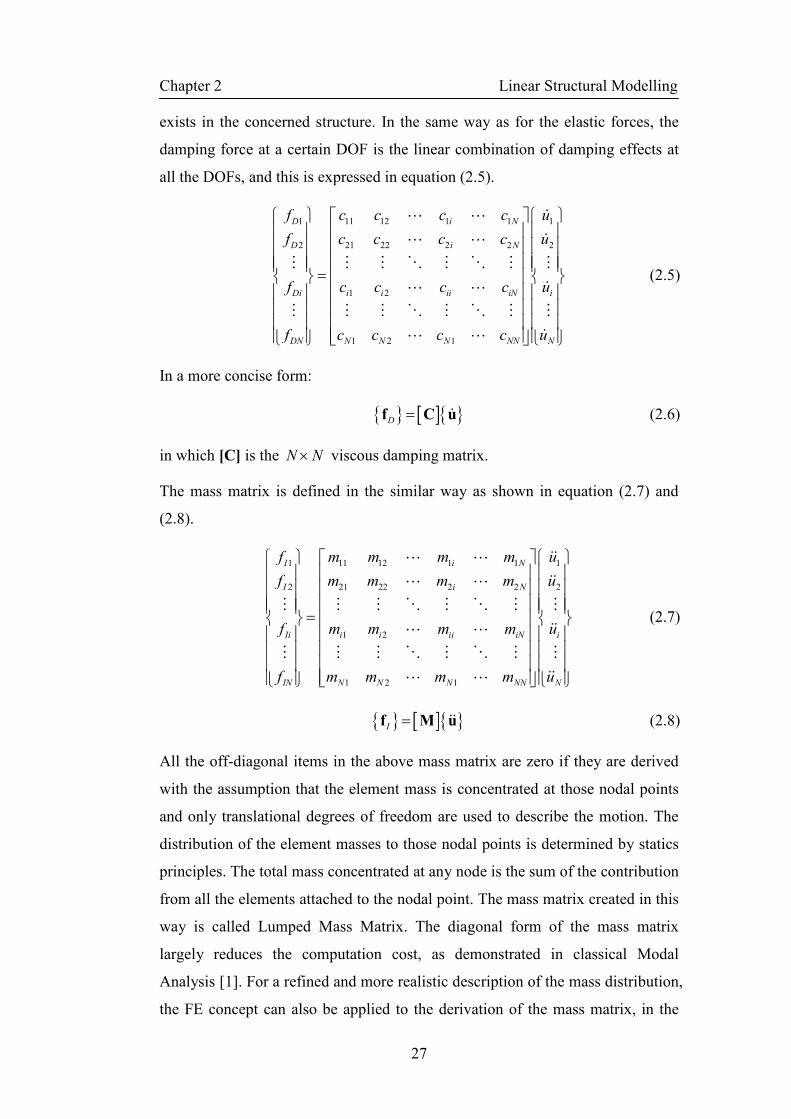
exists in the concerned structure. In the same way as for the elastic forces, the
damping force at a certain DOF is the linear combination of damping effects at
all the DOFs, and this is expressed in equation (2.5).
1 11 12 1 1 1
2 21 22 2 2 2
1 2
1 2 1
D i N
D i N
Di i i ii iN i
DN N N N NN N
f c c c c u
f c c c c u
f c c c c u
f c c c c u
=
ɺ⋯ ⋯
ɺ⋯ ⋯
⋮ ⋮ ⋮ ⋱ ⋮ ⋱ ⋮ ⋮
ɺ⋯ ⋯
⋮ ⋮ ⋮ ⋱ ⋮ ⋱ ⋮ ⋮
ɺ⋯ ⋯
(2.5)
In a more concise form:
[ ] f C uD = ɺ (2.6)
in which [C] is the N N× viscous damping matrix.
The mass matrix is defined in the similar way as shown in equation (2.7) and
(2.8).
1 11 12 1 1 1
2 21 22 2 2 2
1 2
1 2 1
I i N
I i N
Ii i i ii iN i
IN N N N NN N
f m m m m u
f m m m m u
f m m m m u
f m m m m u
=
ɺɺ⋯ ⋯
ɺɺ⋯ ⋯
⋮ ⋮ ⋮ ⋱ ⋮ ⋱ ⋮ ⋮
ɺɺ⋯ ⋯
⋮ ⋮ ⋮ ⋱ ⋮ ⋱ ⋮ ⋮
ɺɺ⋯ ⋯
(2.7)
[ ] f M uI = ɺɺ (2.8)
All the off-diagonal items in the above mass matrix are zero if they are derived
with the assumption that the element mass is concentrated at those nodal points
and only translational degrees of freedom are used to describe the motion. The
distribution of the element masses to those nodal points is determined by statics
principles. The total mass concentrated at any node is the sum of the contribution
from all the elements attached to the nodal point. The mass matrix created in this
way is called Lumped Mass Matrix. The diagonal form of the mass matrix
largely reduces the computation cost, as demonstrated in classical Modal
Analysis [1]. For a refined and more realistic description of the mass distribution,
the FE concept can also be applied to the derivation of the mass matrix, in the

Chapter 2 Linear Structural Modelling
28
same way as the stiffness matrix, in which appropriate shape functions are put
into use.
Substituting equations (2.4), (2.6) and (2.8) into (2.2), we have the fundamental
system equation that governs the dynamic behaviour of the modelled structure.
[ ] [ ] [ ] M u + C u + K u = fɺɺ ɺ (2.9)
Mathematically, equation (2.9) represents a coupled system of linear second
order ordinary differential equations. The matrices [M], [C] and [K] represent
the Spatial model of the structure.
2.2.2 Modal Model
Without any external excitation each structure’s dynamic behaviour is unique
and can be described by a set of natural frequencies and the corresponding
vibration mode shapes. Both sets of values can be derived from the calculation
of the steady-state solution of equation (2.9) when f 0= . For demonstration
purposes, the damping matrix [ ]C is set at [ ]0 .
It can be assumed that u Ui te ω= when the structure is vibrating naturally, in
which U is the 1N × vector of time-independent amplitudes of the response.
Rearranging equation (2.9):
2K M U 0i te ωω − = (2.10)
The only non-trivial solutions are those which satisfy:
2det 0K Mω− = (2.11)
The solution of this equation is N values of 2ω , the undamped system’s natural
frequencies. Substituting each of the natural frequencies back into equation (2.10)
yields a corresponding set of relative values of response amplitudes ψr , the
so-called mode shape corresponding to that natural frequency [1]. In
mathematical expression, these two sets of values are represented in matrix form
as:

Chapter 2 Linear Structural Modelling
29
2
1
2
1
0
0
Ω
Ψ ψ ψ ψ
N
r N
ω
ω
=
=
⋯
⋮ ⋱ ⋮
⋯
⋯ ⋯
(2.12)
They are called eigenvalues and eigenvectors respectively, and form the Modal
model of a structure.
2.2.3 Response Model
As the name itself indicates, this type of model describes how a structure
responds under a given excitation. On the surface, the response depends not only
on the structure’s inherent properties but also on the amplitude of the imposed
excitation. However, it is found that for linear structures specifically, the ratio
between the response and excitation is unique to the structure under study. It can
also be derived analytically from the system equation (2.9) by substituting
u Ui te ω= and f F
i te ω= into it. Setting [ ] [ ]=C 0 and rearranging the
equation into:
( ) 1
2U K M F H Fω ω−
= − = (2.13)
in which ( )H ω is the so-called Receptance matrix of the system with the size
of N N× and is a representation of the Response model. Each entry of the
Receptance matrix is defined as:
( ) j
jk
k
UH
Fω
=
(2.14)
The response jU is a displacement; it can also be in the form of velocity or
acceleration. The ratio between the response and the external excitation is known
as the Frequency Response Function (FRF). In this thesis, ( )H ω will be
referred to as the FRF matrix.
2.2.4 Finite Element Method
The Finite Element Method (FEM) is a modelling and numerical analysis
technique for obtaining approximate solutions to a wide variety of engineering
problems. In the field of structural dynamics, it involves creating a mathematical
Chapter 2 Linear Structural Modelling
30
model of a material or design that is stressed and analysed to assess its dynamic
properties. It is a well-developed method and is widely used in industry in the
process of new product design, refinement of existing products, etc. FEM is
being discussed here because it provides a vigorous mathematical foundation, as
well as a physical interpretation of the application of the Spatial model. In
addition, the dynamic analysis of complex structures nowadays relies on the
FEM to generate the Spatial model for further processing.
The label Finite Element Method first appeared in a paper on plane elasticity
problems by Clough [3] in 1960, but the ideas of finite element analysis date
back much further into 1940s, and were developed independently across
different scientific communities with different purposes and prospects. In the
engineering community, this method was originated from physical intuition that
a continuum structure could be analogised with a truss problem by dividing the
structure into elements or structural sections interconnected at only a finite
number of node points [4]. More developments followed, which concentrated on
finding improved ways to discretise the structure to yield better results [5]. This
method only took off seriously in the late 1950s when automatic digital
computation emerged and opened the way to the numerical solution of complex
problems, which had previously been hindered by the amount of numerical
calculations involved. Engineers began to recognise the efficacy of the Finite
Element Method, and it has been receiving widespread acceptance ever since.
This was further fuelled by the advancement in Personal Computer and the
introduction of many commercial software packages that are developed based on
the concept of FEM, notably a few big names: ABAQUS
, MSC/NASTRAN
and ANSYS
, which is used in the modelling work in this thesis.
Regardless of which software package being used, the solution of a continuum
problem by the Finite Element Method always follows an orderly step-by-step
process as described in [5]:
1. Discretise the continuum
2. Select interpolation equation
3. Define element properties
4. Assemble element properties to obtain the system equations
Chapter 2 Linear Structural Modelling
31
5. Impose the boundary conditions
6. Solve the system equations
7. Make additional computation if required
The modern FEM software packages make Finite Element Analysis a relatively
easy task compared with twenty years ago; however, by no means does this
imply that the requirement for the user to understand FEM is of any less
importance. Computer Aided Design (CAD) is now integrated in the FEM
software package, which allows the analysis of structures with complex
geometries. The discretisation is accomplished by defining a mesh density or
mesh size along a line, surface or solid, and the software will automatically fill
the continuum with elements. The user is responsible for choosing the most
suitable element type, which governs the interpolation equations to be applied by
the software, as well as the final system assembly equation that represents the
structural model. Material properties, boundary and loading conditions,
numerical algorithms and results presentation format need to be defined before
engaging the software into computation.
FEM is today still the dominant method for obtaining approximate solutions of
many engineering problems, and its development is still a hot topic in both
research and industry fields. Efforts made in improving iterative solvers and
error indicators, implementing special-purpose elements and applying meshless
formations can be found in many commercial software packages [5].
2.2.5 Remarks on Different Types of Linear Structural Models
Spatial, Modal and Response models of the same structural component are
interrelated. It is possible to progress from the Spatial model through to a
Response model with the application of FEM and solving the constitutional
equations either in the frequency domain or in the time domain. It is also
possible to carry out an analysis in the reverse direction – to derive Modal and
Spatial models from the Response properties, which are normally obtained from
vibration tests. The interdependence of these three representations of a structural
component forms the linkage between test and simulation.
The Modal model is the most concise one among the three in terms of the
amount of information it carries. It contains only the key information of a
Chapter 2 Linear Structural Modelling
32
structure’s dynamic properties as far as the steady-state solution is concerned.
Because of this, Modal properties are most often used to compare the likeness of
the analytical model and experimental model of the same structure. This topic
will be further explored in the next section.
2.3 Model Validation
The purpose of creating analytical models is economically driven. It is meant to
reduce the design cycle time, and cut down the capital spending on fabrication
and testing of prototypes. However, if the analytical model has not been
validated, there will be no assurance to confirm that it can reliably represent the
real structure and be used in further design stages. From the structural dynamics
point of view, the validated analytical model should be able to predict the
dynamic behaviour of the structure at the experiment condition. It should also be
able to predict, with certain accuracy, the dynamic properties of the structure in
situations different to those in which the experiment was undertaken [6]. To
achieve this, the first step is to make a direct and objective comparison of
specific dynamic properties, measured versus predicted. This is followed by
making adjustments or modifications to one set of results, normally the predicted
one, to bring them closer to each other. When this is achieved, the analytical
model can be said to have been validated an is fit to be used for further analysis
[7].
Up to this point, we can define model validation as a process of determining and
attaining the ‘correct’ parameters of an analytical model so that it can provide an
acceptably correct description of the real structure’s dynamic behaviour. It is a
process that should be performed at every stage of the modelling of a complex
structure. It should start from the component level, and this is the reason for it
being discussed here.
2.3.1 Model Correlation
The simulation results from the analytical model need to be compared with
experimental data of the same structure to assess its suitability for further
process. The discrepancies between these two sets of data may be quantified and
used as a reference to modify the analytical model. The whole business about

Chapter 2 Linear Structural Modelling
33
assessing the likeness between the analytical and experimental models of the
same structure is referred to as model correlation.
As far as the dynamic properties are concerned, natural frequencies, mode
shapes and response properties are used for comparison.
2.3.1.1 Comparison of natural frequencies
The most obvious comparison to make is the measured versus the predicted
natural frequencies. It is not a process as straightforward as it seems, because in
many cases it is not correct to compare directly the modes that are identified in
experiment and prediction in the same sequential order. The reasons are: firstly,
there are modes that are only registered in either experiment or prediction;
secondly, there are modes which have very close natural frequencies though they
have totally different vibration patterns. Therefore, it is essential to identify
associated mode pairs before comparing the corresponding natural frequencies.
The association between experimental and predicted modes is based on the
degree of similarity of the vibration patterns of the compared mode pairs.
The result of the comparison is represented in the form of Natural Frequency
Difference (NFD), which is normally taken percentage-wise and used as a
reference for model updating.
2.3.1.2 Comparison of mode shapes
It is stated in the previous section that comparing the natural frequencies alone is
not enough, unless of course the structure is very simple and all the modes are
well separated. Otherwise we need to perform a comparison of the mode shapes
that are derived from experiment and prediction. Mode shapes describe the
relative position of selected points on a structure for a given vibration mode.
Each vibration mode has its unique mode shape, and if the structure is linear the
mass normalised mode shapes are supposed to be orthogonal to each other. This
leads to the concept of Modal Assurance Criterion (MAC), which quantifies the
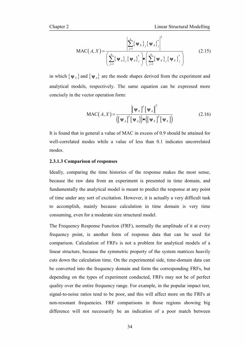
likeness of a pair of mode shapes. It is defined as:
Chapter 2 Linear Structural Modelling
34
( )
2
*
1
* *
1 1
MAC ,
ψ ψ
ψ ψ ψ ψ
n
X Aj jj
n n
A A X Xj j j jj j
A X=
= =
=
•
∑
∑ ∑ (2.15)
in which ψ X and ψ A are the mode shapes derived from the experiment and
analytical models, respectively. The same equation can be expressed more
concisely in the vector operation form:
( )[ ] [ ]
[ ] [ ]( ) [ ] [ ]( )
2
MAC ,
T
X A
T T
A A X X
A X =•
ψ ψ
ψ ψ ψ ψ (2.16)
It is found that in general a value of MAC in excess of 0.9 should be attained for
well-correlated modes while a value of less than 0.1 indicates uncorrelated
modes.
2.3.1.3 Comparison of responses
Ideally, comparing the time histories of the response makes the most sense,
because the raw data from an experiment is presented in time domain, and
fundamentally the analytical model is meant to predict the response at any point
of time under any sort of excitation. However, it is actually a very difficult task
to accomplish, mainly because calculation in time domain is very time
consuming, even for a moderate size structural model.
The Frequency Response Function (FRF), normally the amplitude of it at every
frequency point, is another form of response data that can be used for
comparison. Calculation of FRFs is not a problem for analytical models of a
linear structure, because the symmetric property of the system matrices heavily
cuts down the calculation time. On the experimental side, time-domain data can
be converted into the frequency domain and form the corresponding FRFs, but
depending on the types of experiment conducted, FRFs may not be of perfect
quality over the entire frequency range. For example, in the popular impact test,
signal-to-noise ratios tend to be poor, and this will affect more on the FRFs at
non-resonant frequencies. FRF comparisons in those regions showing big
difference will not necessarily be an indication of a poor match between
Chapter 2 Linear Structural Modelling
35
analytical and experiment models. Signal-to-noise ratios can be improved if
other types of experiment are carried out, e.g. sine sweep test etc. Another
difficulty in FRF comparison is that FRFs are very sensitive to geometric
information, more specifically, to the exact location of excitation and response.
It is found that two FRFs relating to two response points that are very close to
each other on the same structure can be very different [7].
In nonlinear structural modelling, FRFs can be the only feasible choice for
comparison to assess the dynamic properties. As we shall see in future chapters
that even for a weak nonlinearity, the FRFs are distorted considerably, while in
the time domain, the distortion may be hard to notice or in any way deemed to be
meaningful.
2.3.2 Model Updating
After the model correlation, if the discrepancies are small and within the error
margin due to the limitations in the construction of analytical model and
experiments conducted on the physical structure, the analytical model can be
passed as suitable for further processing, e.g. joining to other analytical models
to form an assembly. Otherwise, some adjustment has to be made in order to
bring the analytical model closer to the experimental one. This process is called
model updating. This subject has become a very extensive one, with already one
textbook [8] and several hundred papers devoted to its details [9]. Some of the
concepts and methods have been well developed and applied successfully in
many cases. This section is more meant to show the importance of model
updating, and how it is employed in the process of achieving good assembly
model in the end.
Broadly speaking, there are two types of model updating methods. The first one
is called the Direct Matrix Method, in which the individual elements of the
system matrices M, C and K are adjusted directly according to the comparison
between the test data and analytical model prediction. This type of method has
the advantage of being computationally straightforward and can be very efficient
in matching closely the dynamic properties. However, physical interpretations
can hardly be drawn from the direct matrices adjustment. The other type of
method, generally called Indirect Method, is where the physical properties of the

Chapter 2 Linear Structural Modelling
36
model are adjusted instead. The physical properties can be material-related, e.g.
density and Young’s modulus, or geometry-related. Change of these properties
will indirectly change the system matrices, so is the prediction result. This type
of method gives more physical sense to the analytical models that need to be
updated.
Throughout these years there are many algorithms proposed to implement the
concept of model updating. Very detailed surveys can be found in the following
references [6, 10, 11]. One of the most popular methods is summarised here,
which is also applied in this thesis for updating component models.
2.3.2.1 Inverse eigensensitivity method
This method is one type of the Indirect Method approach. Its calculation is based
on the initial dynamic properties of the model and the first order sensitivity
function of those properties. The fully-fledged mathematical derivation is very
lengthy. A simplified version, which is sufficient for updating simple component
models, is presented here.
This method attempts to minimise the discrepancy between corresponding pairs
of natural frequencies, also known as eigenvalues, from the experiment and
analytical model prediction. The following penalty function is normally used,
assuming only one parameter p is updated:
( ) ( )( )2
1
( )m
A Xi ii
J p ω ω=
= −∑ (2.17)
where ( )A iω and ( )X i
ω are the ith
corresponding analytical and experimental
eigenvalues, while ( )J p is a function of updating parameter p. Using Taylor
series to expand the above equation and truncate those items of second order and
above, we will have:
( )( )
( )0
2
1
( )m
A iA p p Xi i
i
J p pp
ωω δ ω=
=
∂ ≅ + −
∂ ∑ (2.18)
where, p0 is the initial value of the updating parameter, and δp is the increment
of the updating parameter, which will be decided during the updating process. A
Chapter 2 Linear Structural Modelling
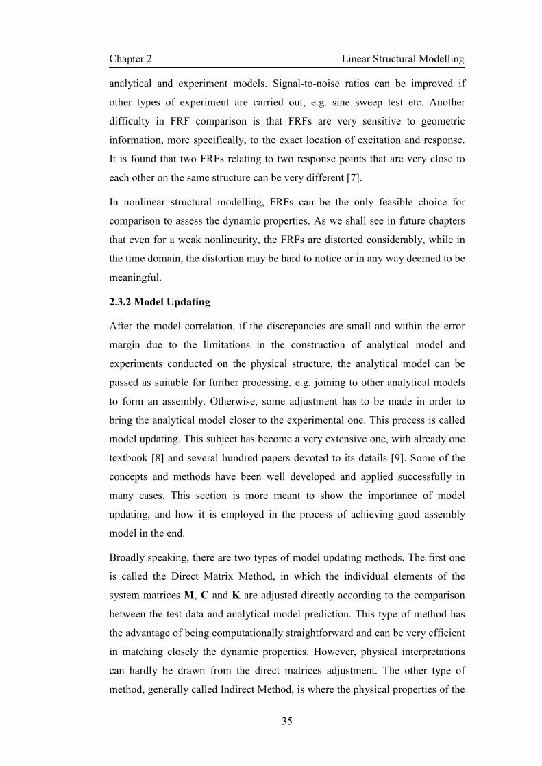
37
minimum value of J can be achieved if we partial-differentiate the above
equation with respect to δp and set the new equation equal to 0:
( )
( )( )
( )( )
0
1
2 0m
A Ai iA p p Xi i
i
Jp
p p p
ω ωω δ ω
δ ==
∂ ∂ ∂≅ × + − =
∂ ∂ ∂ ∑ (2.19)
Further simplifying the above equation, we will have:
( )
( ) ( )A iX Ai i
pp
ωδ ω ω
∂= −
∂ (2.20)
Considering all the mode pairs we can write the above equation in matrix form:
[ ] S p Rω ωδ = (2.21)
In which [ ]Sω is called the sensitivity matrix of the eigenvalues with respect to
the updating parameter. R Ω ΩX Aω = − is the residual vector between the
experiment eigenvalues and the predicted ones. To derive the unknown pδ ,
the sensitivity matrix needs to be inverted. This is where the name for this kind
of methods is derived. Eigenvalues are usually non-linear functions with respect
to almost all kinds of updating parameter [6]; hence equation (2.21) can only be
solved iteratively.
2.3.3 Remarks on Model Validation
Model validation is an extensive topic and still in the course of development.
This section presents the philosophical background of this topic and is meant to
raise the awareness that model validation is an essential part of structural
dynamic modelling, even though it may seem tedious and in certain cases rather
additional to an already adequate model. As the Finite Element Method,
computing power and operator’s modelling skills get improved continuously, we
can now sometimes make an analytical model that matches the experiment close
enough to achieve the required accuracy in prediction without any adjustment,
but at what kind of confidence level can we safely take in an analytical model
without any experimental validation? There have not been any rules that can
reliably answer this question. Model validation is still the safest and yet
necessary step in every stage of structural dynamic modelling.

Chapter 2 Linear Structural Modelling
38
Model validation must start at the component level. The argument is always the
same: without accurate component models, we will not feel confident in the final
assembly model. A case study of component model validation will be shown in
Chapter Seven, in which a cylindrical casing model has been improved by
applying Inverse Eigensesitivity method upon the experimental result.
Last but not least, a meaningful and successful model validation relies on good
experiment practice. This topic will be touched upon in Chapter Six.
2.4 Linear Structural Coupling Techniques
After the component models have been properly validated, the next step is to
join them together to form an assembly, and this falls into another large topic in
structural dynamics: structural coupling. It is also sometimes known as
substructure analysis. This branch of structural dynamic analysis originated
during the time when computing power was still limited and the demand for
modelling of more complex structure was growing. It was known that for an N
degree-of-freedom system, the CPU effort for an eigensolution is approximately
proportional to N3. Therefore if the system is subdivided into two equal
subsystems the solution time may be expected to be reduced by a factor of 4 [12].
Therefore, lots of effort was devoted to developing new techniques to take
advantage of such properties to improve the computation efficiency.
Besides time saving, there are other advantages that attributes to the fast
development in this field. Firstly, the problem of modelling a complex structure
can be greatly simplified by dividing the structure into substructures where each
substructure can be better represented by a smaller, more accurate and refined
mathematical model [13]. Secondly, with proper coupling techniques, it is
possible to couple models from different sources, for example to couple an
analytical model with experiment model. In today’s product development field,
complex machines are finely dissected into small segments and each are studied
in detail. Modifications tend to be at the very local level. With suitable coupling
techniques, the integration between different parts can be operated more
smoothly and economically.
Structural coupling is also closely linked to model reduction, a topic in structural
dynamics that concentrates on reducing the complexity of the problem definition
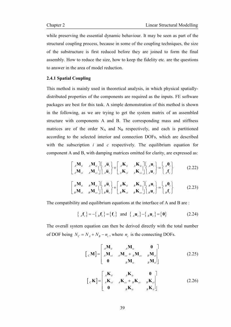
Chapter 2 Linear Structural Modelling
39
while preserving the essential dynamic behaviour. It may be seen as part of the
structural coupling process, because in some of the coupling techniques, the size
of the substructure is first reduced before they are joined to form the final
assembly. How to reduce the size, how to keep the fidelity etc. are the questions
to answer in the area of model reduction.
2.4.1 Spatial Coupling
This method is mainly used in theoretical analysis, in which physical spatially-
distributed properties of the components are required as the inputs. FE software
packages are best for this task. A simple demonstration of this method is shown
in the following, as we are trying to get the system matrix of an assembled
structure with components A and B. The corresponding mass and stiffness
matrices are of the order NA and NB respectively, and each is partitioned
according to the selected interior and connection DOFs, which are described
with the subscription i and c respectively. The equilibrium equation for
component A and B, with damping matrices omitted for clarity, are expressed as:
M M u K K u 0
M M u K K u f
A ii A ic A i A ii A ic A i A i
A ci A cc A c A ci A cc A c A c
+ =
ɺɺ
ɺɺ (2.22)
M M u K K u 0
M M u K K u f
B ii B ic B i B ii B ic B i B i
B ci B cc B c B ci B cc B c B c
+ =
ɺɺ
ɺɺ (2.23)
The compatibility and equilibrium equations at the interface of A and B are :
and f f f u u 0A c B c c A c B c= − = − = (2.24)
The overall system equation can then be derived directly with the total number
of DOF being C A B cN N N n= + − , where cn is the connecting DOFs.
[ ]M M 0
M M M M M
0 M M
A ii A ic
C A ci A cc B cc B ci
B ic B ii
= +
(2.25)
[ ]K K 0
K K K K K
0 K K
A ii A ic
C A ci A cc B cc B ci
B ic B ii
= +
(2.26)
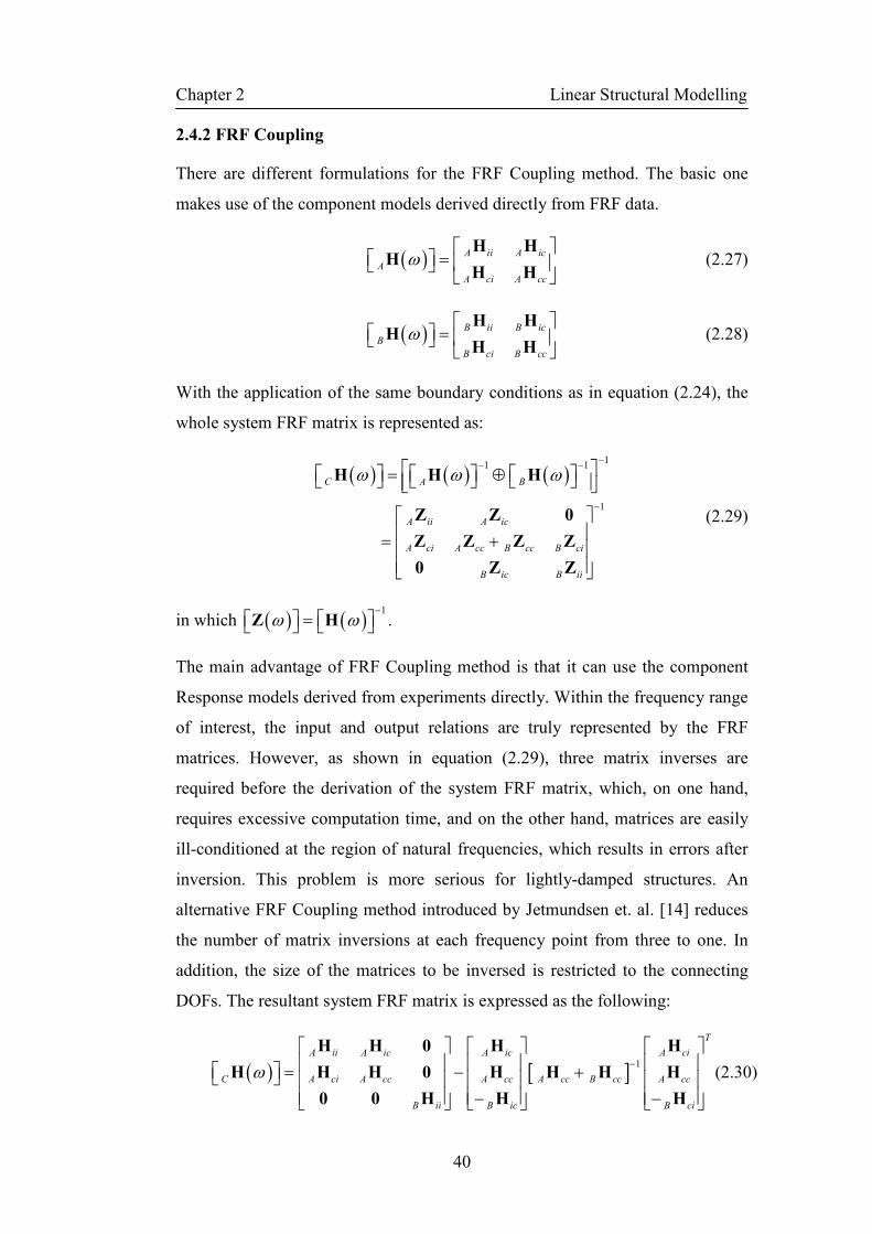
Chapter 2 Linear Structural Modelling
40
2.4.2 FRF Coupling
There are different formulations for the FRF Coupling method. The basic one
makes use of the component models derived directly from FRF data.
( )H H
HH H
A ii A ic
A
A ci A cc
ω
=
(2.27)
( )H H
HH H
B ii B ic
B
B ci B cc
ω
=
(2.28)
With the application of the same boundary conditions as in equation (2.24), the
whole system FRF matrix is represented as:
( ) ( ) ( )1
1 1
1
H H H
Z Z 0
Z Z Z Z
0 Z Z
C A B
A ii A ic
A ci A cc B cc B ci
B ic B ii
ω ω ω−− −
−
= ⊕
= +
(2.29)
in which ( ) ( )1
Z Hω ω−
= .
The main advantage of FRF Coupling method is that it can use the component
Response models derived from experiments directly. Within the frequency range
of interest, the input and output relations are truly represented by the FRF
matrices. However, as shown in equation (2.29), three matrix inverses are
required before the derivation of the system FRF matrix, which, on one hand,
requires excessive computation time, and on the other hand, matrices are easily
ill-conditioned at the region of natural frequencies, which results in errors after
inversion. This problem is more serious for lightly-damped structures. An
alternative FRF Coupling method introduced by Jetmundsen et. al. [14] reduces
the number of matrix inversions at each frequency point from three to one. In
addition, the size of the matrices to be inversed is restricted to the connecting
DOFs. The resultant system FRF matrix is expressed as the following:
( ) [ ] 1
H H 0 H H
H H H 0 H H H H
0 0 H H H
T
A ii A ic A ic A ci
C A ci A cc A cc A cc B cc A cc
B ii B ic B ci
ω−
= − + − −
(2.30)

Chapter 2 Linear Structural Modelling
41
2.4.3 Modal Coupling
Modal coupling methods are also called Component Mode Synthesis (CMS).
The first CMS method was proposed by Hurty [15]. Depending on the boundary
conditions applied to the substructure interfaces, the CMS methods can be
classified into four groups: fixed interface methods; free interface methods;
hybrid interface methods and loaded interface methods. Reviews of these
methods can be found in [16] and [17]. The formulation of fixed interface
method is summarised here. The dynamic equation at the component level is:
M M u K K u f
M M u K K u f
ii ic i ii ic i i
ci cc c ci cc c c
+ =
ɺɺ
ɺɺ (2.31)
It is assumed that the connecting interface is fixed and there is no force applied
to all the internal DOFs, i.e. u 0c = and f 0i = . The corresponding
equation of motion becomes:
[ ] [ ] M u K u 0ii i ii i+ =ɺɺ (2.32)
This can be solved to deduce eigenvalues [ ]iΩ and eigenvectors [ ]iΨ of this
fixed interface structure. The internal DOFs can be represented by the linear
combination of the known fixed interface modes as:
[ ] i i i=u Ψ p (2.33)
The displacement of internal DOFs also has the contribution from the connection
DOFs, boundary modes or restrained modes as they are normally called. In this
case, the relationship is described by Guyan reduction [18]. Hence, a
transformation matrix can now be constructed, which is commonly known as
Craig-Bampton method:
[ ]u p pΨ Ψ
Tu u u0 I
i i ii ic
c c c
∗ = =
(2.34)
where ic
∗ Ψ is the Guyan transformation matrix and it is defined as:
[ ] [ ]1
ic ii ic
−∗ = − Ψ K K (2.35)

Chapter 2 Linear Structural Modelling
42
It is common, especially for experimentally derived models where there are only
k number of modes available, that the above equation still can be used to count
for all the physical DOFs:
[ ]u p pΨ Ψ
Tu u u0 I
i ik ikik ic
k
c c c
∗ = =
(2.36)
Substitute equation (2.36) into (2.31) and pre-multiply [ ] 1Tk
−, with some tedious
but straightforward mathematical transformation, we can finally get the
combined system equation as the following:
I 0 M p Ω 0 0 p 0
0 I M p 0 Ω 0 p 0
M M M M u 0 0 K K u 0
A kk A kc A ik A ik A ik
B kk B kc B ik B ik B ik
A ck B ck A cc B cc c A cc B cc c
+ = + +
ɺɺ
ɺɺ
ɺɺ
(2.37)
The above method can further be improved by including other types of modes,
e.g. attachment modes, rigid body modes [19] and improved boundary modes
[20] etc. to improve the accuracy.
2.4.4 Practical Consideration in Applications
The two prime considerations that drive the development of structural coupling
techniques are computational efficiency and prediction accuracy. It is always a
trade-off situation between these two objectives. In order to increase
computational speed, the complexity of the problem must be reduced, which
means some ‘non-important’ information, for example some DOFs and/or
vibration data at high frequencies which are not relevant, must be sacrificed in
order to reduce the amount of information that needs to be processed. The
consequence is a reduced quality of the prediction results: less information and
less accuracy. As far as the outcome is concerned, if there is enough
computational power, full size modelling is always preferred.
The abovementioned structural coupling techniques do not necessarily require
the component size to be reduced before they are joined. It is acceptable to keep
the component model intact and to use the same interface constraints and
equations for the coupling. This, however, still will not guarantee a good quality
assembly model, because a key part is not represented sufficiently here: the joint.

Chapter 2 Linear Structural Modelling
43
It has generally been considered as rigid in those formulations. There are
attempts being made to consider joints as elastic media [21], and in fact it is
treated in the same way as the other structural components, being modelled as an
individual entity.
The Finite Element Method is by far the most common way to construct an
analytical structural model, so it is natural to use it to construct the joint model
also. Actually in a rather isolated way FEM has already been used in studying
the behaviour of various types of joints: bolted, welded, bonded etc. [22, 23],
though all the studies concentrated on their static behaviour only. A joint is
quite a complicated mechanism as will be shown in the next chapter. Thousands
of DOFs may be need to model a single joint in order to acquire its nonlinear
micro and macro stick-slip behaviour, for example. It is of course too much of a
burden to try to incorporate this kind of massive joint model into the assembly
model in studying the dynamic behaviour.
If, however, the joint can be assumed to be linear, it can be modelled as a simple
layer of finite elements between the connected components. The element
material properties can be adjusted to reflect the joint’s correct flexibility and
this can be achieved by carrying out a model updating exercise on the joint FE
model only. In Chapter Seven, a linear structural coupling example is presented
with experimental validation. The bolted joints are represented by a layer of FE
elements. Their properties are updated via experiment.
The FE joint model is limited to linear case if the eigensolution or steady-state
response is of the interest, because any nonlinearity in the FE definition has to be
discarded in order to take the advantage of symmetric property in the system
matrices when calculating the eigensolutions. If the nonlinearity cannot be
neglected, some special algorithms must be used to derive the steady state
solution in order to avoid the time-consuming time-domain calculation.
2.5 Concluding Remarks
This chapter is effectively an overview of a field that has already been well
developed. It might seem to be basic, but it is crucial to get the fundamentals
right before we embark on more complicated problems. The linear assumption is
still largely used and actually it is acceptable in most applications. Methods and

Chapter 2 Linear Structural Modelling
44
techniques to perfect linear component models are crucial in achieving good
final assembly model. Mechanical joints, even though their behaviour is better
described as nonlinear, can often still be considered as linear at normal operation
conditions, and linear coupling methods can be used efficiently to produce
acceptable results.
Even though the theories have been well laid out, the actual application can be
tricky and depends a lot on the thorough understanding of the subject.

Chapter 3 Nonlinear Joint Modelling
45
Chapter 3
Nonlinear Joint Modelling 3.1 Introduction
The modern mechanical system design theory [24] states that an assembly
represents an idea or concept greater than the sum of the individual parts. This
indicates the direction for modern machinery development: innovative
combinations of ever more number of specialised individual parts. To achieve so,
various types of connection mechanisms are needed to properly link the
individual parts into a functional assembly. From the structural modelling point
of view, these jointed connections can be in different physical forms so long as
the kinetic and kinematic constrains are considered properly, which is of course
the difficult part of joint modelling.
Joints are normally treated separately from the remaining structural components.
One of the reasons is that it is impossible to have a generalised joint model. This
is in contrast to the structural components that can all be modelled by defining
the mass, stiffness and damping matrices from the design data with FEM, or
frequency response data from experiment. This has been well developed, and can
be applied to all kinds of components, regardless of size and geometric
complexity. In order to be incorporated into a whole assembly mathematical
model, the joints need to be described with the same type of kinetic constraints

Chapter 3 Nonlinear Joint Modelling
46
as those in the FE description of the structural component models. The physics
of such constraints is rather different, and in some cases it is difficult to come up
with a mathematical description without significant simplification. One typical
example is a friction joint, the model of which is still more or less derived
approximately from the experiment.
Joints are major sources of nonlinearity in an assembly. This is also part of the
reason why joints should be treated separately from other components. The
natural way of tackling this problem is to work from linear to non-linear in joint
description. If linear joint models and normal structural coupling techniques can
solve the problem within the required accuracy, there is no need to go for
nonlinear methods. It is, however, necessary to deploy nonlinear models and
calculation methods when the experimental results show discrepancies with
simulations which can not be improved by merely enhancing the linear models
and methods.
The concept of nonlinearity will be explored in detail in the next chapter. Briefly
speaking, the fundamental difference between a linear system and a nonlinear
one is that the latter’s behaviour is not simply the sum of its parts or their
multiples, as it is in a linear system. In mathematical terms, the rules of
superposition and proportionality are true to linear systems but not to nonlinear
ones. This difference is at the root of all the difficulties involved in nonlinear
problems.
In the realm of nonlinear joint modelling, two issues are of particular concern.
Firstly, extra care should be taken when a joint must be considered to be
nonlinear. This is, of course, not to undermine the importance of linear joint
modelling. The fact is that nonlinear models need more parameters to describe
the behaviour sufficiently. In a linear system, less joint parameters are required
and they can be easily adjusted based on the discrepancies between the
experiment and simulation data. The same is difficult to do in a nonlinear system
because of the large number of unknown parameters. Secondly, a nonlinear joint
model must be presented in a form that is ready to be integrated with the
remaining structural component models. This normally means a simplification of
the joint model, even though in order to capture all the nonlinear phenomenon,
Chapter 3 Nonlinear Joint Modelling
47
more parameters and conditions should be included in the description. To
summarise, nonlinear joint models should be representative and concise.
There are two ways to obtain a nonlinear joint model. One is from the study of
the fundamental physics of the joint, and the other is from expriment. The latter
is known in the engineering world as ‘parameter identification’, which focuses
on the reconstruction of the unknown governing equations of the joint. Both
approaches have been carried out rather independently by physicists and
engineers. It is nowadays believed that hybrid techniques that utilise both
analytical and experimental data produce more reliable and accurate joint models
[13].
This chapter focuses on a few representative nonlinear joint models which are
commonly encountered in mechanical engineering, ranging from friction-
induced nonlinearity to geometric nonlinearity. The main purpose is to raise
awareness of the importance of joint modelling, and the complicated nature of it.
Before embarking on the various detailed models, a list of different joint types is
presented.
3.1.1 Joint Types
According to Maloney et al. [25], from the joint’s effect on structural response
point of view, joints can be broadly categorized into non-separable and separable
joints. The former tends to be stronger, stiffer, more consistent and more
predictable. Examples include welded joints [26, 27] and soldered joints [28].
This type of joint is mostly modelled with Finite Elements, and the concerns in
research are more on their long-term reliability than on simulation of normal
working conditions. Separable joints are often more difficult to predict and
sensitive to many parameters that cannot readily be specified or controlled.
There is a long list of separable joints that are presented in different physical
forms: bolted joints, rivets, pin joints, thread connections, expansion joints, etc.
[29-31].
The difficulties in modelling these separable joints are mainly caused by the
existence of friction between the two joining parts. Friction provides resistance
force against the relative movement and in fact this is how the joints bind the
whole assembly together. Friction phenomena have been studied for centuries,

Chapter 3 Nonlinear Joint Modelling
48
and the primary cause is yet to be fully understood by physicists. Mechanical
engineers are keen on developing representative models from experiments,
which should be accurate enough to represent the joint in its specific operating
conditions. The friction joints will be discussed in detail in the following section.
It is also common to define some secondary components of an assembly, like
angles, plates, gussets, gaskets and bearings as joints. They can indeed be
modelled together with the other components, but depending on the computation
capacity available and accuracy requirement for the whole assembly, these
secondary components can be represented by joint models. A ball bearing in
rotating machinery, for instance, connecting the rotor and stator, can be
modelled as an individual structural component, containing details of sub-
assemblies like balls, inner race, outer race etc. However, it can also be modelled
as a simple mass-spring model connecting the rotor and stator, provided this
simplification does not deteriorate the simulation quality.
3.2 Nonlinear Joint Models
3.2.1 Friction Models
Friction provides resistance to relative motion between two contacting bodies.
This phenomenon is easy to perceive but difficult to model, and it is indeed not
yet completely understood of its fundamental causes even today. Many types of
joint can be stripped down to frictional elements. Some notable examples are
bolted joints, fasteners, friction dampers and bearings etc. Friction has been
studied extensively in classical mechanics, and at various times, numerous
friction models, both phenomenological and empirical, have been proposed to
provide predictive capabilities. One of the aims is to simplify the description of
friction, with as few parameters as possible, in order to incorporate it easily with
the rest of the structure in modelling the whole system; while at the same time
the friction model itself is sufficient to replicate what is observed from
experiment, even if it may lack physical insight in some cases.
In this section, the fundamentals about friction are first reviewed, which are
followed by a few representative friction models most often seen in literature.
Some of the main literature reviews on this subject can be referred to papers [32-
34].
Chapter 3 Nonlinear Joint Modelling
49
3.2.1.1 Friction Phenomenon
Experience with friction is as old as human history, but it was not until the
Renaissance period when Leonardo Da Vinci first conducted controlled
experiment to observe and quantify friction, that the phenomenon started
attracting attentions of generations of scientists and engineers till today. In his
famous static friction experiment with a block on horizontal and inclined planes,
Da Vinci concluded that the force needed to start one object sliding over another
is proportional to the force that presses the two objects together, but independent
of the area of contact. This was later found out to be a not-so-accurate
description, because the friction force does depend on the area of contact from
the microscopic point of view. Nevertheless this is the first time the friction
phenomenon was characterised.
From a structural dynamics point of view, we are more interested in the effect of
friction on the whole assembly dynamic behaviour and therefore, the observable
friction phenomenon, or macroscopic friction, are of concern and need to be
quantified. From Da Vinci, macroscopic friction laws have since been enriched
by Amontons, Euler, Coulomb and in more recent times notably by Bowden and
Tabor [35]. Some of the typical frictional phenomena are summarised below:
Static friction and break-away force. Static friction is the friction when
sticking. The friction force opposes the direction of motion when the sliding
velocity is zero, and it is equal to the externally applied tangential force until
a maximum is reached. The break-away force is the tangential force required
to initiate relative motion of two contacting bodies. It was found that the
break-away force depends not only on the relative displacement between two
contact surfaces, but also on the increment rate of the external force.
Coulomb friction. For most engineering materials, the friction force
between the two sliding surfaces is constant as long as relative motion
continues. The force level only depends on the materials of the two bodies
and the pressing force. This phenomenon was first documented by Amontons
(1699) and Coulomb (1785).
Viscous friction. This is the friction phenomenon observed when lubricant is
used between two contacting surfaces. It was conclude by Reynolds (1866)

Chapter 3 Nonlinear Joint Modelling
50
that the friction force caused by the viscosity of lubricants is proportional to
the relative velocity of the two sliding surfaces.
Micro-slip and Macro-slip. When two surfaces in contact slide against each
other, localised deformation and slippage occurs before observable slide
takes place. The stage when there is no relative motion between the two
contacting surfaces is called micro-slip, and is widely observed in friction
damping problems. Once the external force parallel to the interface surface
exceeds the breakaway force level, relative motion will occur. This is called
macro-slip. In some engineering applications, e.g. loose bolt joints under
cyclic excitation, micro-slip and macro-slip happen repeatedly. This is
known as stick-slip cycle. It is a major nonlinear source in assembly
structures with bolted joints.
3.2.1.2 Friction Mechanisms
We are more interested here in the manifestation of friction, and a mathematical
representation of it; nevertheless, it is also interesting and useful to know the
underlying physical properties. As we know friction is the tangential reaction
force between two surfaces in contact. Physically, these reaction forces are the
result of many different mechanisms which depend on contact geometry and
topology, properties of the bulk and surface materials of the bodies,
displacement and relative velocity of the bodies and the presence of lubrication
[36]. Some of the mechanisms are [36, 37]:
In dry sliding contacts between flat surfaces, the elastic and plastic
deformation of microscopic asperities in contact causes the resistance force,
i.e. the friction force. It is accepted as a general rule that for each asperity
contact, the tangential deformation is elastic until the applied shear pressure
exceeds the shear strength of the surface material, when it becomes plastic.
The break-away of the asperities finally leads to slip when the externally
applied tangential force is large enough.
In dry rolling contact, the frictional force is the result of a non-symmetric
pressure distribution in the contact, and this uneven distribution is caused by
elastic hysteresis in either of the contact bodies.

Chapter 3 Nonlinear Joint Modelling
51
When lubricants are added to the contact, the friction force is affected by the
viscous property of the lubricant, the relative velocity of contacting surfaces,
pressure and thickness of lubricant film, etc. Depending on the different
combinations of the above physical properties, different mechanisms
dominate in the inception of friction force. For example, at high velocity and
low pressure, the friction is determined by the shear force built up in the fluid
layer due to the hydrodynamic effects.
Contamination also needs to be considered sometimes. The presence of small
particles between the contact surfaces give rise to additional forces that
strongly depend on the size and material properties of the contaminations.
There are many more different mechanisms, in addition to the above, cause
friction. To construct a general friction model from physical principles is simply
not possible [36]. Approximate models exist for certain configurations. These
models were constructed based on the observations of friction phenomena.
3.2.1.3 Some Representative Friction Models
Though surface mechanics is useful knowledge, in the context of structural
mechanics, however, such a detailed knowledge of surface mechanics is not
always necessary. All we are looking for are the equivalent spring and damping
forces displayed by a friction joint. Some of the mostly referred models in the
literature are presented below.
Coulomb Friction Model
This is by far the most common model used to describe dry contact friction. It is
widely used because of its simplicity and good approximation from the
macroscopic point of view. The mathematical expression between the friction
force f and relative velocity v can be written as:
0
0
0
N v
f F v
N v
µ
µ
>
= =− <
(3.1)
in which:
F is the external force;
µ is the dynamic friction coefficient;

Chapter 3 Nonlinear Joint Modelling
52
N is the normal clamping force;
Graphically, it is represented in Figure 3 - 1.
Figure 3 - 1 The Coulomb friction model
The above classical friction models can not capture the behaviour when there is
relative velocity between the contacting surfaces. What is more, it neglects the
small displacements that occur at the contacting interface during stiction.
Therefore, as far as structural dynamics is concerned, a friction model involving
dynamics is necessary for accurate description of the friction phenomena [38].
The following few models take care of the dynamic properties of the frictional
joints.
1-D Jenkins Model
It is found from experiment that when the friction joint is under dynamic
excitation, the joint response is similar to the elasto-plastic response of metals
[34]. One of the simplest models to describe such a material property is the
Jenkins spring slider element, which has also been successfully implemented in
friction joint modelling.
Each Jenkins model consists of a spring and a Coulomb slider element, which
has two possible arrangements, in series or in parallel as shown in Figure 3 - 2(a)
and (b), respectively. In the case of Figure 3 - 2(a), the Coulomb element is
connected in series with the spring element. Under a cyclic external excitation,
the Coulomb element is firstly in its sticking state at the beginning of each cycle,
which provides a resistive force equal and opposite to the input force to the
µN
-µN

Chapter 3 Nonlinear Joint Modelling
53
element, while the spring element provides the displacement representing micro-
slip. When the friction capacity of the Coulomb element is passed, the sliding
state starts. Once in the sliding state the Coulomb element provides constant
resistance of magnitude equal to the coefficient of friction multiplied by the
normal force. The typical force-displacement representation of this type of
Jenkins model is shown in Figure 3 - 3. In the case of parallel connection of
Coulomb element and spring element, as shown in Figure 3 - 2(b), the
corresponding characteristic curve is shown in Figure 3 - 4.
(a) In series (b) In parallel
Figure 3 - 2 Symbolic representation of Jenkins model
Figure 3 - 3 Characteristic curve of a Jenkins model with elements in series
Figure 3 - 4 Characteristic curve of a Jenkins model with elements in parallel
F
u
F
u
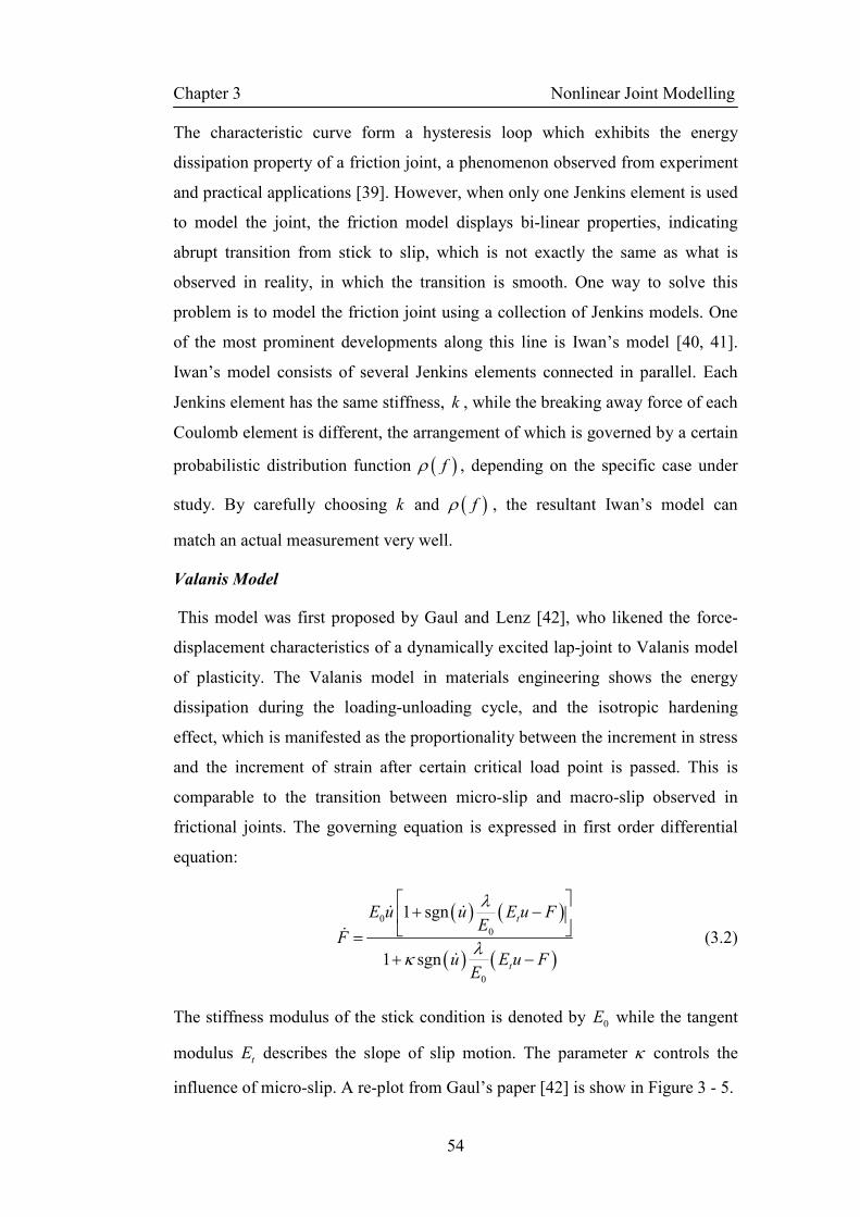
Chapter 3 Nonlinear Joint Modelling
54
The characteristic curve form a hysteresis loop which exhibits the energy
dissipation property of a friction joint, a phenomenon observed from experiment
and practical applications [39]. However, when only one Jenkins element is used
to model the joint, the friction model displays bi-linear properties, indicating
abrupt transition from stick to slip, which is not exactly the same as what is
observed in reality, in which the transition is smooth. One way to solve this
problem is to model the friction joint using a collection of Jenkins models. One
of the most prominent developments along this line is Iwan’s model [40, 41].
Iwan’s model consists of several Jenkins elements connected in parallel. Each
Jenkins element has the same stiffness, k , while the breaking away force of each
Coulomb element is different, the arrangement of which is governed by a certain
probabilistic distribution function ( )fρ , depending on the specific case under
study. By carefully choosing k and ( )fρ , the resultant Iwan’s model can
match an actual measurement very well.
Valanis Model
This model was first proposed by Gaul and Lenz [42], who likened the force-
displacement characteristics of a dynamically excited lap-joint to Valanis model
of plasticity. The Valanis model in materials engineering shows the energy
dissipation during the loading-unloading cycle, and the isotropic hardening
effect, which is manifested as the proportionality between the increment in stress
and the increment of strain after certain critical load point is passed. This is
comparable to the transition between micro-slip and macro-slip observed in
frictional joints. The governing equation is expressed in first order differential
equation:
( ) ( )
( ) ( )
0
0
0
1 sgn
1 sgn
t
t
E u u E u FE
F
u E u FE
λ
λκ
+ −
=+ −
ɺ ɺ
ɺ
ɺ
(3.2)
The stiffness modulus of the stick condition is denoted by 0E while the tangent
modulus tE describes the slope of slip motion. The parameter κ controls the
influence of micro-slip. A re-plot from Gaul’s paper [42] is show in Figure 3 - 5.
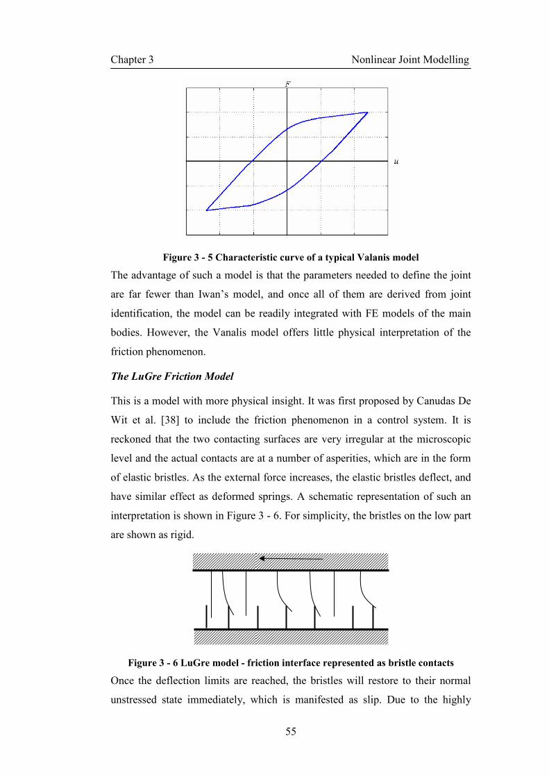
Chapter 3 Nonlinear Joint Modelling
55
Figure 3 - 5 Characteristic curve of a typical Valanis model
The advantage of such a model is that the parameters needed to define the joint
are far fewer than Iwan’s model, and once all of them are derived from joint
identification, the model can be readily integrated with FE models of the main
bodies. However, the Vanalis model offers little physical interpretation of the
friction phenomenon.
The LuGre Friction Model
This is a model with more physical insight. It was first proposed by Canudas De
Wit et al. [38] to include the friction phenomenon in a control system. It is
reckoned that the two contacting surfaces are very irregular at the microscopic
level and the actual contacts are at a number of asperities, which are in the form
of elastic bristles. As the external force increases, the elastic bristles deflect, and
have similar effect as deformed springs. A schematic representation of such an
interpretation is shown in Figure 3 - 6. For simplicity, the bristles on the low part
are shown as rigid.
Figure 3 - 6 LuGre model - friction interface represented as bristle contacts
Once the deflection limits are reached, the bristles will restore to their normal
unstressed state immediately, which is manifested as slip. Due to the highly
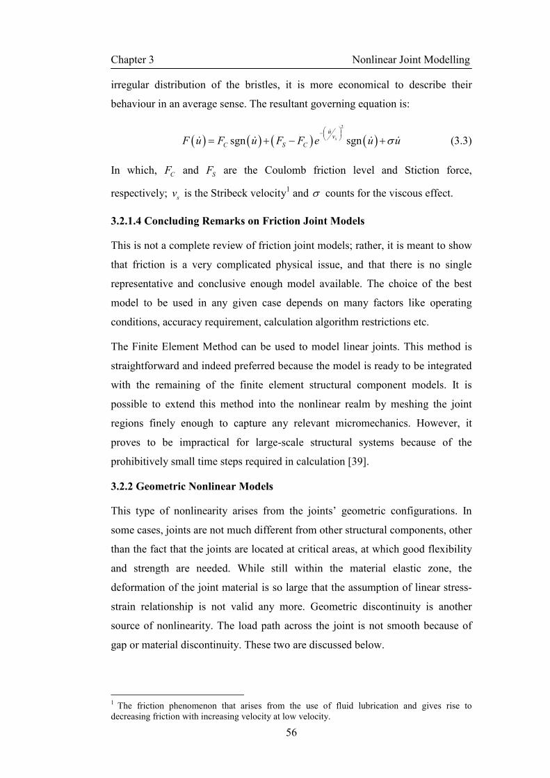
Chapter 3 Nonlinear Joint Modelling
56
irregular distribution of the bristles, it is more economical to describe their
behaviour in an average sense. The resultant governing equation is:
( ) ( ) ( ) ( )2
sgn sgns
uv
C S CF u F u F F e u uσ − = + − +ɺ
ɺ ɺ ɺ ɺ (3.3)
In which, CF and SF are the Coulomb friction level and Stiction force,
respectively; sv is the Stribeck velocity1 and σ counts for the viscous effect.
3.2.1.4 Concluding Remarks on Friction Joint Models
This is not a complete review of friction joint models; rather, it is meant to show
that friction is a very complicated physical issue, and that there is no single
representative and conclusive enough model available. The choice of the best
model to be used in any given case depends on many factors like operating
conditions, accuracy requirement, calculation algorithm restrictions etc.
The Finite Element Method can be used to model linear joints. This method is
straightforward and indeed preferred because the model is ready to be integrated
with the remaining of the finite element structural component models. It is
possible to extend this method into the nonlinear realm by meshing the joint
regions finely enough to capture any relevant micromechanics. However, it
proves to be impractical for large-scale structural systems because of the
prohibitively small time steps required in calculation [39].
3.2.2 Geometric Nonlinear Models
This type of nonlinearity arises from the joints’ geometric configurations. In
some cases, joints are not much different from other structural components, other
than the fact that the joints are located at critical areas, at which good flexibility
and strength are needed. While still within the material elastic zone, the
deformation of the joint material is so large that the assumption of linear stress-
strain relationship is not valid any more. Geometric discontinuity is another
source of nonlinearity. The load path across the joint is not smooth because of
gap or material discontinuity. These two are discussed below.
1 The friction phenomenon that arises from the use of fluid lubrication and gives rise to
decreasing friction with increasing velocity at low velocity.

Chapter 3 Nonlinear Joint Modelling
57
3.2.2.1 Cubic Stiffness
This is probably the most documented nonlinearity in structural dynamics. As
the demand for faster, lighter and more efficient machine increases, some parts
of such a structural assembly may undergo deformation so large that the
relationship between force and displacement is no long a constant. It is possible
that this type of nonlinearity is due to plastic deformation of the base material,
but it is more common in practice that the base material is flexible and designed
to work in its elastic region, and the only nonlinear source is the assumption of
the infinite small deformation is no long valid in constructing the stress-strain
relationship.
The stiffness nonlinearity can be analytically formulated and numerically
simulated using FEM. The resultant equation to describe the relation between the
force and the displacement can be written as:
3
1 3F k u k u= + (3.4)
This characteristic is known as the cubic stiffening effect, and is best
demonstrated with Figure 3 - 7. As the load F is increased steadily, the
deflection increment gets less and less. If we take equivalent stiffness at every
point along the curve, it is easy to see that the equivalent stiffness gets larger as
the deflection increases.
F F F F
u
Figure 3 - 7 Characteristic plot of a typical cubic stiffness

Chapter 3 Nonlinear Joint Modelling
58
3.2.2.2 Polynomial Stiffness
For a real structure experiencing large deflection, the stiffness function may
include not only a cubic term but also higher-order terms in which the cubic term
may dominate. There also exists in engineering application a cubic nonlinear
stiffness with a negative first order term [43, 44], as 1 0k < in equation (3.4).
Graphically the characteristic curve for this case is as shown in Figure 3 - 8:
A B O
F
u
Figure 3 - 8 Characteristic curve of cubic stiffness with negative linear term
This is an interesting nonlinear case. Globally, it represents the case of stiffening
spring. Locally, it has negative linear stiffness at its global centre O, and a
weakening stiffness at its two static equilibrium points, A and B. The weakening
effect can be visualised from the above plot. As the displacement leaves the
equilibrium point and approaches the global centre, there is more and more
deflection for a steadily increased load, until arriving at the point where the
deflection is extreme for a very small increase in load. This local nonlinear
stiffness can be fitted with a second order polynomial curve. In later chapters, it
will be shown with an example that a slightly buckled beam possesses this type
of nonlinearity.
3.2.2.3 Piecewise Linear Stiffness
This type of nonlinearity is caused by geometric discontinuity between two
connecting components. It has a practical interest in many mechanical systems,
such as the stiffness in the clutch of automobile power transmission system,
backlash in the gear system, etc. A universal piecewise linear stiffness model is
Chapter 3 Nonlinear Joint Modelling
59
shown in Figure 3 - 9(a) with different linear stiffness values at different
displacement stages. There are two special cases worth mentioning here.
Piecewise Linear Stiffness
Bi-Linear Stiffness
Clearance
F
u u
F
u
F
k1
k2
k1
k2
k3
k1
k2
k1
(a) (b) (c)
Figure 3 - 9 Piecewise linear stiffness models
Figure 3 - 9(b) shows a bi-linear stiffness case. One practical example is the
bolted flange connection [45], in which the dominant stress-strain direction is
along the bolt centre line. The stiffness 1k in the compression regime is
relatively higher because the compression load is shared by both the bolt stud
and the flange; while the stiffness 2k in the tension regime is smaller because the
tensile load is only borne up by the bolt stud. Other bi-linear joint examples can
be found in loosely joint structures [46].
Figure 3 - 9(c) shows a clearance type of nonlinearity. In some mechanical
assemblies, a clearance is inevitable at the joint. Small suitable clearance is
necessary to move a mechanism smoothly. In addition, through wear-and-tear, a
small gap may be built up, e.g. the rattling problem in a gear system. Another
example can be found in the application of Active Magnetic Bearing (AMB)
systems in rotating machinery, in which an emergency ‘catcher’ bearing is used
to support the rotor when the AMB is not functioning. It is a complicated
problem involving impact mechanisms and rubbing etc., but it can be simplified
and represented by a clearance type of joint as shown above. Here 2 0k =
reflects the non-contact status.
3.3 Concluding Remarks
A few representative joint models have been presented in this chapter. The aim
is to provide manageable joint models to the whole assembly model. It should be

Chapter 3 Nonlinear Joint Modelling
60
noted that a joint is often extremely difficulty to model using a purely analytical
approach. It always relies on experimental data to validate and correct the
mathematical models. This is a research subject in its own right, known as joint
identification. A large number of techniques have been proposed, notably
collected in annual IMAC1 and biennial ISMA
2 conferences.
1 International Modal Analysis Conference 2 International Conference on Noise & Vibration Engineering

Chapter 4 Dynamic Analysis of Nonlinear Structures
61
Chapter 4
Dynamic Analysis of Nonlinear
Structures 4.1 Introduction
Some forms of nonlinearity have been presented in the previous chapter when
different structural joint models are described. From those various graphs that
depict the relation between two parameters, e.g. displacement and restoring force,
it is found that the relationship is not linearly proportional, as otherwise would
be described by a straight line. This is the manifestation of nonlinearity that we
most appreciate. The definition of nonlinearity can be expressed with a more
stringent mathematical sense: the fundamental rule that judges whether a system
is linear or nonlinear, is the conformance of the following two principles [47]:
• The principle of superposition;
• The principle of proportionality.
Violating either one means the existence of nonlinearity. This is because in a
linear condition, the system is described by linear differential equations, which
are the summation of dependent variables and their derivatives. Doubling the
external excitation leads to doubling the responses, and the individual response
Chapter 4 Dynamic Analysis of Nonlinear Structures
62
to each excitation components can simply be summed up to get the total
response. In nonlinear situation, this is not true.
The existence of nonlinearity in a structure can be due to many different
mechanisms, some of which have been covered in the previous chapter, but there
is a long list to follow, and most of them are case-based. It is rather difficult to
neatly categorise different types of nonlinearity based on its physical properties.
It is, however, possible to classify the nonlinearity based on its extent: global
nonlinearity and localised nonlinearity [13]. The former is found in problems
related to nonlinear material properties; and the latter, which is to be focused on
in this thesis, exists at the connection between two adjoining components,
usually known as a joint. The large part of the remaining structure is effectively
linear. This inspired the introduction of methods that take advantage of the
localised properties of the nonlinearities to speed up the calculation for such type
of structure on which nonlinearity only exists at a small number of DOFs. In this
chapter we shall first examine a few methods that solve general nonlinear
problems, which do not differentiate these two types of nonlinear problems in
structural dynamics.
The principles of superposition and proportionality are the cornerstones of linear
theory. Various analytical methods have been developed to make full use of
these principles to simplify the process of solving problems of a linear system.
The analytical solutions are described in algebraic form without the inclusion of
numerical values for parameters. Once the solutions are obtained, any desired
numerical values can be inserted and the entire possible range of solutions can be
explored, which is certainly a time-saving practice, in addition to its exactness.
Nonlinear structural dynamic problems are usually described by nonlinear
differential equations, which can be notoriously difficult to solve in an analytical
closed form. The existence and co-existence of many interesting nonlinear
phenomena, e.g. bifurcation, sub-harmonic and super-harmonic motion, limited
cycle and chaos, means that a direct analytical solution is indeed not possible.
Therefore, indirect or approximation procedures must be applied.
There are two major branches in the modern developments of nonlinear analysis:
the analytical methods of successive approximations and the topological
methods of graphical integration [48]. The latter one originated from the

Chapter 4 Dynamic Analysis of Nonlinear Structures
63
graphical representation of the solution of dynamic equilibrium equations in the
phase plane. Phase planes are useful for visualising the behaviour of a physical
system. Stability and unique vibration patterns can be assessed through the study
of the integral curves in the phase planes. However, these methods are only
applicable to lower order systems and are mostly used in the more
mathematically inclined approaches. The concept of phase plane will be
demonstrated in a later section. The main purpose of this thesis is to develop
accurate and efficient structural modelling practices for large-scale structure
assemblies; hence, only the first type of these methods is going to be
investigated in more detail. Some of the important methods to find approximate
analytical solutions are (i) the perturbation method, (ii) the iteration method, (iii)
the averaging method, (iv) the harmonic balance method [48] and the step-by-
step direct numerical integration of the differential equation in the time-domain
method [13]. These can be grouped into two categories, time-domain methods
and frequency-domain methods.
This thesis focuses on finding steady-state solutions of a nonlinear structure
subjected to periodic excitation. It is understood from linear structural dynamic
analysis that the dynamic properties of a linear system can be characterised by a
set of frequency response functions, which relate the amplitude and phase of the
response to harmonic excitation. This concept can be extended to nonlinear
structural dynamic analysis to study how a nonlinear structure responds to
harmonic excitation. It is noted that cyclic external excitation is very often
experienced by engineering structures, e.g. vibration caused by unbalanced
rotating machinery, so to analyse the steady-state solution of a structure
subjected to periodic excitation has clear physical significance. In addition, from
the model validation point of view, if the steady-state response calculation can
be correlated with experiment, it will prove that the nonlinear structure is
correctly modelled.
In the following sections, time-domain methods and frequency-domain methods
are discussed. The focus is on the Runge-Kutta Method and Harmonic Balance
Method respectively, which are used in the subsequent case study. This case
study is an interesting one DOF nonlinear problem with a ‘strange’ nonlinear
stiffness. A large collection of steady-state solutions have been found.

Chapter 4 Dynamic Analysis of Nonlinear Structures
64
4.2 Time-Domain Analysis
‘Time-domain’ is a term used to describe the analysis of mathematical functions
or physical signals, with respect to time. In this thesis, we refer this type of
analysis as those numerical methods for solving ordinary differential equations
with time as the independent variable. The signal or the state of a system is
calculated step-by-step throughout the time history at discrete points.
In the case of using Spatial model to represent the structure, a set of differential
equations are applied to describe the dynamic equilibrium at each DOF. For a
linear system, the exact steady-state solution of this set of equations can be
solved by an analytical method with respect to time. They can also be solved
numerically to get approximate solutions at discrete time points. With carefully-
selected time step size and a numerical calculation scheme, the result will be
very close to the exact analytical solution. In linear case, numerical schemes are
not preferred because it is far more expensive to run them.
For studying the dynamic response of a nonlinear structure, the analytical
solution is extremely difficult to get. Time-domain numerical schemes are
among the many procedures used to find the corresponding approximate
solutions. They are renowned for being potentially accurate, even though a low
computational efficiency is still unavoidable. In this thesis, we focus on
examining efficient approximate methods to describe a nonlinear system under
periodical external excitation. Time-domain calculation results will be used as
the ‘exact’ solution, to be compared with those from other approximate methods.
4.2.1 Runge-Kutta Method
The fourth-order Runge-Kutta method is one of the standard algorithm to solve
differential equations. No knowledge is required about the nonlinear system and
it virtually always succeeds with reasonable accuracy [13]. This method is
designed to imitate the Taylor series method without requiring analytic
differentiation of the original differential equations [49]. The dynamic system
can be described with the following second order differential equations:
[ ] [ ] [ ] [ ] M u C u D u K u g fi+ + + + =ɺɺ ɺ (4.1)

Chapter 4 Dynamic Analysis of Nonlinear Structures
65
in which, g is the nonlinear internal force vector. In order to accommodate the
application of the numerical method, this second-order equation needs to be re-
written into first order form:
[ ] [ ] [ ] [ ] u v
M v C v D u K u g fi
=
+ + + + =
ɺ
ɺ (4.2)
The above equation can be arranged in a single matrix form as:
i
+ =
M 0 v C K+ D v f-g
0 I u I 0 u 0
ɺ
ɺ (4.3)
This is most commonly written in the state-space equation format as:
( ) z S ,zt=ɺ (4.4)
in which:
v u
zu u
= =
ɺ (4.5)
and
( ) 1
it
−
= −
M 0 f-g C K+ D vS ,z
0 I 0 I 0 u (4.6)
When the initial conditions 0( )z t is known, equation (4.4) is ready to be solved
by the Runge-Kutta formulations:
( ) ( ) ( )1 2 3 42 26
ht h t+ = + + + +z z R R R R (4.7)
in which:
( )
( )
1
2 1
3 2
4 3
1 1
2 2
1 1
2 2
t
t h h
t h h
t h h
+
+
+
=S ,z
=S , z+
=S , z+
=S , z+
R
R K
R K
R K
(4.8)
Chapter 4 Dynamic Analysis of Nonlinear Structures
66
and h is the time step size defined by the user. The derivation of the above
formulation can be found in standard textbooks [50].
The Runge-Kutta Method has been well developed theoretically and proven to
be accurate and efficient. It is a standard component in various mathematical
software packages, and many variations exist to cater for users’ different
priorities and some uncommon problems. In this thesis, MATLAB
is adopted
as the platform to carry out time domain analysis. ode45 is the key command
used, which implements the above-presented 4th
order Runge-Kutta method. In
general, this command is the first function to try for most problems [51]. One
point needs to be noted: MATLAB
uses variable step size for the calculation.
This is achieved by estimating the error at every calculation step, comparing the
error with the pre-defined tolerance and altering the step size accordingly. It is of
course possible to fix the step size h by the user even though it is not advisable.
The danger with applying fixed time step size is that if the oscillation period of
the input signal is smaller than the time step, crucial dynamic information would
totally be missed in the results. In addition, solving with fixed step size tends to
be slower comparing to those with variable step size, because if the input signal
changes gently, the step size can be relatively coarse without sacrificing the
accuracy.
4.2.2 Other Time-domain Methods
The Runge-Kutta Method is one type of the so-called ‘Explicit’ numerical
methods. The name comes from the fact that the current state of a system is
calculated using the information from the state of the system at the previous time
step. Other methods in the same category are: Forward Euler Method, Central
Difference Methods, Taylor Series Schemes, Predictor-Corrector method, [52,
53] etc. These methods are suitable for small scale problems in terms of the
order of the system equation, and problems concerning medium to high
frequency range of a structure, like those shockwaves response simulation in
impact tests. The stability of these type of methods is the main concern. The time
step size needs to be inversely proportional to the highest vibration frequency
inherent to the structure, which, if not totally impractical, is extremely small for
Chapter 4 Dynamic Analysis of Nonlinear Structures
67
a finely meshed FE model. Nevertheless, this type of method is a faster choice, if
the model is relatively small.
Contrary to the Explicit Method, the so-called Implicit Method finds the solution
of the current state of a system by solving an equation involving both current and
previous states of the system. A few notable methods in this category are:
Newmark [54], Wilson-θ [55] and Houbolt methods [53, 56, 57]. These methods
are more suitable for large scale problems and most effective when the
concerned vibration of the structure is characterised by a relatively small number
of low frequency modes [56]. Transient Analysis in many commercial FE
packages uses this type of method, for both linear and nonlinear problems. The
application of these methods becomes much simpler with those user-friendly FE
software packages, in which the user is guided through choices of parameters
that are relevant to particular types of problem. Of course, the user must
understand the fundamentals in the first place.
4.3 Frequency-Domain Analysis
‘Frequency-domain’ is a term used to describe the analysis of mathematical
functions or signals with respect to frequency. A time-domain analysis shows
how a signal changes over time, whereas a frequency-domain analysis shows
how much of the signal lies within each given frequency band over a range of
frequencies. If the described signal is periodic, the frequency-domain
representation is much more concise, because it needs only a few values to
quantify the signal.
A major shortcoming of the time-domain methods is that they are very time-
consuming. The computing time required depends on the scale of the structure
and accuracy requirement. A small time step is needed if explicit methods are
used, as it is inversely proportional to the highest frequency of the structural
model. In addition, if the main concern is to obtain the steady-state solution, the
calculation must be carried on until any transient effect has died away. In the
case of lightly damped structure, this means consuming a significant computing
resource on something which is not intrinsically useful. So alternatively,
frequency-domain approximation methods for determining the steady-state
Chapter 4 Dynamic Analysis of Nonlinear Structures
68
response of structures, particularly to periodic external excitation, should be used,
in which there is no need to analyse transient motion [13].
The limitation of the frequency-domain methods is what time-domain analysis is
strong at: versatility. Some of the most important frequency-domain methods are
presented here, all of which assume steady-state periodic response to periodic
external excitation.
4.3.1 Perturbation Method
This method can actually be applied in both time domain and frequency domain.
It is included here because it can be used to derive steady-state periodic solutions.
Perturbation theory is a century-old, and indeed one of the oldest methods used
to find approximate solution to a nonlinear problem that cannot be solved
exactly. It starts with the assumption that the nonlinear term adds a slight
deviation from the solution of the underlying linear problem, which can be
solved exactly with an analytical method. One of the techniques is to express the
desired solution in terms of a power series of a small perturbation parameter that
quantifies the deviation from the exact solution [58], as shown in the following
equation:
2
0 1 2
2 2 2
1 2
( ) ( ) ( ) ( )
n
u t u t u t u tε ε
ω ω εω ε ω
= + + +
= + + +
⋯
⋯ (4.9)
in which, ε is the perturbation parameter; 0 ( )u t and nω would be the known
solution to the underlying solvable linear problem; 1 2( ), ( ),u t u t ⋯ and
1 2, ,ω ω … are higher order solutions representing small deviations due to the
nonlinearity; and they can be found iteratively. The closeness to the exact
solution depends on the number of higher order terms included in the calculation.
This method is only valid when the real solution is close to that of the underlying
linearised problem, which implies that this method is mainly for systems with
weak nonlinearity.
4.3.2 Describing Functions
The describing function method was first developed to solve nonlinear problems
in control systems [59]. The similarity of the mathematical expressions of a
Chapter 4 Dynamic Analysis of Nonlinear Structures
69
control system and a structural dynamic system inspired the application of this
method in the modelling of a nonlinear structure. This method linearises the
nonlinearity by defining a transfer function that relates the fundamental
harmonic components of the input and the output to the nonlinearity [13]. The
mathematical derivation is briefly shown below, following the approaches of
Tanrikulu et al. [60] and Ferreira [13]. The standard Spatial model is used, with a
term representing nonlinear interaction force included:
[ ] [ ] [ ] ( ) ( ) ( ) ( ) ( ) ( ), ( )t t t t t t+ + + =M u C u K u g u u fɺɺ ɺ ɺ (4.10)
in which, ( ) ( ), ( )t tg u uɺ is the nonlinear interaction force; and ( ) tf is the
external periodic excitation. The kth
element of the nonlinear interaction force is
a combination of the interaction forces between DOF k and all other DOFs. This
can be expressed in summation form:
1
N
k kj
j
g p=
=∑ (4.11)
in which kjp is a function of the inter-coordinate displacement, kjy , and its time
derivatives, and is expressed as:
( ),kj kj kj kjp p y y= ɺ (4.12)
in which:
kj k jy u u= − (4.13)
The external harmonic force with an angular velocity ω can be written as:
( ) i tt e ω=f F (4.14)
It is assumed that the response to the harmonic excitation is also periodic, and
can be expanded in the form of Fourier series:
1
( ) n in t
n
t e ω∞
=
=∑u U (4.15)
It should be noticed that both F and nU are complex vectors with the size of the
total number of DOFs.

Chapter 4 Dynamic Analysis of Nonlinear Structures
70
If the nonlinearity is weak, the fundamental component in the Fourier expansion
of the response is a good assumption of the exact solution:
1( )u U i tt e ω≈ (4.16)
Convert both (4.12) and (4.13) from the time domain to the frequency domain as:
( )1 1i t i t
kj k jY e U U eω ω= − (4.17)
and
( )2
0
1 i t
kj kjP p e d t
πω ω
π−= ∫ (4.18)
The ratio between kjP and kjY is defined as a describing function:
kjkj
kj
Pv
Y= (4.19)
and the complex amplitude of the nonlinear force vector is represented in the
form of the describing function:
1
N
k kj kj
j
G v Y=
=∑ (4.20)
Substitute (4.14), (4.16), (4.20) and (4.17) into (4.10), we will have, after
cancelling the term i te ω− :
[ ] [ ] [ ] [ ]( ) 2 iω ω− + + + =M C K ∆ U F (4.21)
in which [ ]∆ is defined as the generalised quasilinear matrix [60], and its
elements are obtained using the following equations:
( )1
N
kk kj
j
kj kj
v
v k j
=
∆ =
∆ = − ≠
∑ (4.22)
The superscript 1 for the displacement vector U , indicating the fundamental
harmonic is dropped, for clarity. Equation (4.21) can be solved iteratively. When
better accuracy is needed, higher order terms in the Fourier expansion can be
retained, it will however complicate the computation.
Chapter 4 Dynamic Analysis of Nonlinear Structures
71
4.3.3 Harmonic Balance Method
The Harmonic Balance Method (HBM) is a well-known tool for studying
nonlinear dynamic problems in the frequency domain. It can be applied to the
analysis of strongly nonlinear systems, such as the rotor-stator contact problem
[61], and structures with friction contact interfaces [62-64]. The working
principle of this method is that the frequency components of the internal
interaction force must equate to those presented in the response. A set of
balanced equations are therefore derived, one for each frequency component,
which can be solved to get the amplitude and phase of each frequency
component. The implementation is summarised below.
It is first assumed that the steady-state solution is periodic, and can therefore be
expanded into a Fourier series. The assumed solution is then inserted into the
original system dynamic equation. The sine and cosine coefficients of the same
harmonic order are set to zero separately. A set of new equations containing all
the unknown coefficients are subsequently solved. The assumed solution is
finalised in the form of a Fourier series with all the harmonic coefficients
determined. The length of the solution series is determined by the user, and in
general, if more terms of the Fourier series are taken into account, the closer the
approximated solution will be to the exact one. Of course, it requires more
computational effort. The mathematical derivation starts from expressing the
system equation as below, which is the same as equation (4.10):
[ ] [ ] [ ] ( ) ( ) ( ) ( ) ( ) ( ), ( )M u C u K u g u u ft t t t t t+ + + =ɺɺ ɺ ɺ (4.23)
in which, ( ) ( ), ( )g u ut tɺ is the nonlinear internal reaction force; and ( ) f t is
the external periodic excitation. For clarity purpose, the brackets that represent
matrix and vector are omitted in the following mathematical derivations.
Based on the assumption that the response is also periodic, which can be
decomposed with Fourier series as:
0
1
( ) cos sinu U U UN
n n
m m m C m S
n
n nt t t
m mω ω
=
= + +
∑ (4.24)
In which, ω is the frequency of the external harmonic forcing; and m is an
integer corresponding to the ratio of the period of the external forcing to the
Chapter 4 Dynamic Analysis of Nonlinear Structures
72
period of the response. It is used to count for sub-harmonic responses. m=1
when the dominant harmonic in the response is the same as that of the excitation.
Un
m C is the amplitude of the nth
cosine harmonic term, Un
m S is the amplitude of
the nth
sine harmonic term. N is the total number of harmonic terms included in
the Fourier series expansion.
The derivatives of the above equation are:
1
2 2
1
( ) sin cos
( ) cos sin
u U U
u U U
Nn n
m m C m S
n
Nn n
m m C m S
n
n n n nt t t
m m m m
n n n nt t t
m m m m
ω ω ω ω
ω ω ω ω
=
=
= − +
= − −
∑
∑
ɺ
ɺɺ
(4.25)
The nonlinear reaction force is also expressed in a Fourier series:
( ) 0
1
( ), ( ) cos( ) sin( )g u u G G GN
n n
m m m C m S
n
n nt t t t
m mω ω
=
= + + ∑ɺ (4.26)
in which 0 , ,G G Gn n
m m C m S are the respective harmonic terms.
Substitute equation (4.24), (4.25) and (4.26) into (4.23), with a pure sine external
excitation:
2 2
1
1
0
cos sin
sin cos
cos sin
M U U
C U U
K U U U
Nn n
m C m S
n
Nn n
m C m S
n
n n
m m C m S
n n n nt t
m m m m
n n n nt t
m m m m
n nt t
m m
ω ω ω ω
ω ω ω ω
ω ω
=
=
− − +
− + +
+ +
∑
∑
1
0
1
cos( ) sin( ) sin( )G G G F
N
n
Nn n
m m C m S
n
n nt t t
m mω ω ω
=
=
+
+ + =
∑
∑
(4.27)
Balance the harmonic terms on both sides of the equation:
0 0
2
2
. 0
cos( ) 0
1sin( )
0 1
K U G
M U C U K U G
FM U C U K U G
m m
n n n n
m C m S m C m C
n n n n
m S m C m S m S
const
n n nt
m m m
nn n nt
n Nm m m
ω ω ω
ω ω ω
⇒ + =
⇒ − + + + =
= ⇒ − − + + = ≻ ⋯
(4.28)
Chapter 4 Dynamic Analysis of Nonlinear Structures
73
It is noticed from equation (4.26) that Gn
m C and Gn
m S are directly linked with the
response Um ; hence they can be expressed as:
( )( )
0 1 1
0 1 1
, , ,..., ,
, , ,..., ,
G G U U U U U
G G U U U U U
n n N N
m C m C m m C m S m C m S
n n N N
m S m S m m C m S m C m S
=
= (4.29)
Combine equation (4.28) and (4.29) to get 2N algebraic equations with
2N unknown Fourier coefficients of the response.
( )
( )
0 0
2
0 1 1
2
0 1 1
. 0
cos( )
, , ,..., , 0
sin( )
, , ,..., , 0
m m
n n n n N N
m C m S m C m C m m C m S m C m S
n n n n N N
m S m C m S m S m m C m S m C m S
const
nt
m
n n
m m
nt
m
n n
m m
ω
ω ω
ω
ω ω
⇒ + =
⇒
− + + + =
⇒
− − + + − =
K U G
M U C U K U G U U U U U
M U C U K U G U U U U U F
(4.30)
From (4.23) to (4.30), a nonlinear differential equation has been transformed into
a set of nonlinear algebraic equations. With a proper iteration algorithm chosen,
these equations are ready to be solved. The purpose is to find 2N unknowns,
1 1, ,..., ,U U U UN N
m C m S m C m S , with the 2N equations at every frequency point ω .
Equation (4.30) is re-written in matrix form by combining all the harmonic terms:
( ) ( ) ( )- - 0R =Z U F G Uω ω = (4.31)
Where 0 1 1, , , , ,U= U U U U UT
N N
m m C m S m C m S⋯ is a vector of harmonic coefficients
of the response at all system DOFs; ( ) 0 1 1, , , , ,G U G G G G GT
N N
m m C m S m C m C= …
is a vector of harmonic coefficients for all the nonlinear internal forces. ( )Z ω is
similar to the dynamic stiffness matrix of the linear part of the system with
higher harmonic terms included. It is represented as:

Chapter 4 Dynamic Analysis of Nonlinear Structures
74
( )
2
2
2
2
1 1
1 1
K 0 0 0 0
0 K M C 0 0
0 C K M 0 0
Z
0 0 0 K M C
0 0 0 C K M
m m
m m
N N
m m
N N
m m
ω ω
ω ωω
ω ω
ω ω
− − −
= − − −
⋯
⋯
⋯
⋮ ⋮ ⋮ ⋱ ⋮ ⋮
⋯
⋯
(4.32)
Equation (4.31) represents a nonlinear set of equations with respect to U, and the
purpose is to find U at every desirable frequency. If the nonlinear structure under
study has a DOF of sN , the whole set of equations will have ( )2 1sN N× +
unknowns to be decided. One of the most efficient methods for the solution of a
set of nonlinear equations is the Newton-Raphson method which possesses
quadratic convergence when an approximation is close enough to the solution.
The iteration is conducted with the following formula at every frequency point
of interest:
( )1
( )( 1) ( ) ( )R
U U R UU
kk k k
−
+ ∂= − ∂
(4.33)
The superscript (k) indicates the number of the current iteration. Performing
differentiation of equation (4.33) with respect to U, the recurrence formula can
be rewritten in the form:
( )( ) ( )
1( )
( 1) ( ) ( )G U
U U Z R UU
k
k k kω
−
+ ∂ = − + ∂
(4.34)
The derivatives ( )( )
G U
U
k∂∂ are calculated using finite-difference formulae.
One further point needs to be mentioned here is that ( )G U cannot be explicitly
expressed. It needs be calculated every time a new U is derived, with Fourier
coefficient calculation:

Chapter 4 Dynamic Analysis of Nonlinear Structures
75
( ) ( )( )
( ) ( )( )
( ) ( )( )
0
0
0
0
1,
1, cos
1, sin
G g u u
G g u u
G g u u
T
m m m m
T
n
m C m m m
T
n
m S m m m
t t dtT
nt t t dt
T m
nt t t dt
T m
ω
ω
=
=
=
∫
∫
∫
ɺ
ɺ
ɺ
(4.35)
in which T is the external excitation period.
4.4 Case Study
The procedure of using the Harmonic Balance Method to derive steady-state
periodic response of a nonlinear system is applicable to a system of any number
of DOFs. However, for demonstration purposes, only a 1-DOF nonlinear system
is presented in this case study, which is meant to show a special type of
nonlinearity and the fact that HBM can cope with it well.
4.4.1 Problem Definition
We study the nonlinear equation of a 1-DOF oscillator:
( ) ( ) ( ) ( ) ( )3
1 3 sinmu t cu t k u t k u t F tω+ + + =ɺɺ ɺ (4.36)
in which some physical values are assigned for the numerical studies:
m = 1kg; c = 1Ns/m; 1k = -1000N/m; 3k = 10000N/m3; F = 2000N.
The nonlinearity only exists in the restoring spring force, which, with the
assigned physical values, can be visualised with the graph below. It resembles a
slightly buckled beam undergoing forced lateral vibration, as shown in Chapter
Three. This is actually a Duffing’s equation with a negative linear stiffness. A
similar system was first systematically studied by Holmes [65], in response to
the demand from the study of population dynamics and Earth’s magnetic field
model. It has since become an interesting subject for mathematicians.
When the static force 0F = , there are three static equilibrium points, indicated
as O, A and B at 0u = and 0.3162u = ± respectively as shown in Figure 4 - 1.
The non-zero equilibrium points A and B are dynamically stable, while point O
is not, because of the existence of negative stiffness around this global centre.

Chapter 4 Dynamic Analysis of Nonlinear Structures
76
-1 -0.8 -0.6 -0.4 -0.2 0 0.2 0.4 0.6 0.8 1-2000
-1500
-1000
-500
0
500
1000
1500
2000
displacement (m)
force (N)
O A B
Figure 4 - 1 Force-displacement curve of the nonlinear spring
One of the main purposes of this study is to find as many as possible steady-state
periodic solutions for the nonlinear dynamic equation (4.36), and to show that
Harmonic Balance Method is a very efficient alternative to the usual time-
domain methods.
4.4.2 Time-Domain Calculation
The time integration starts from some initial conditions in terms of displacement
u and velocity uɺ . The differential equations are then integrated over a time
interval which is long enough to allow transient effect to disappear and steady-
state vibrations to settle down. A fourth-order Runge-Kutta method with variable
step scheme is used. Various initial conditions are examined in order to find
different steady-state solutions for the same magnitude and frequency of
excitation force. The excitation frequency ranges from 1Hz to 80Hz in a step of
0.1Hz. At each frequency point, 200 runs with randomly selected initial
conditions are conducted.
The result of this exhaustive study is shown in Figure 4 - 2. The maximum
displacement amplitudes over a vibration period of the steady-state response are
shown as functions of the excitation frequency. Each ‘branch’ corresponds to
one type of steady-state periodic response of the system, which is characterised
by the dominant harmonic components in the response. Some branches have
been marked to indicate the dominant harmonics. For example, the branch
marked with ‘1/3, 3/3, …’ contains all the 1/3 sub-harmonic responses. In the

Chapter 4 Dynamic Analysis of Nonlinear Structures
77
frequency range between 18Hz to 32Hz, a cluster of sub-harmonic solutions are
found below the branch of main harmonic response. They will be shown with
more details in next section.
Figure 4 - 2 Steady-state solutions from time-domain integration
4.4.3 Frequency-Domain Calculation
The search for the sub-, super- and major periodic solutions in the frequency
domain was performed for different initial approximations of the periodic
solutions and for different harmonic numbers kept in the multi-harmonic
expansion of the solution. For each calculation, the execution of the algorithm
started with a guess for the harmonic coefficients of the forced response. The
HBM algorithm with a continuation scheme [66] was used, which ensured that
the periodic solutions of the same type were efficiently calculated and traced
along the whole frequency range of interest. Both stable and unstable solutions
can be determined as a result of these calculations. Owing to these features, the
frequency-domain solution process requires only one point close to the trajectory
of solutions in order to calculate the whole trajectory. Hence, the number of the
frequency-domain calculations is smaller by several orders of magnitude than
the number of runs carried out for the time-domain analysis. As a result, the
expense required for frequency-domain calculation is a very small fraction of the

Chapter 4 Dynamic Analysis of Nonlinear Structures
78
time-domain computation expense. The initial approximations for the forced
response spectrum were deduced from some steady-state solutions found in the
time-domain integration.
The results of all these calculations are plotted in Figure 4 - 3, together with the
time-domain calculation results for comparison. The time-domain calculation is
represented with blue dots, and the frequency domain calculation with solid
black lines. The clustered region is enlarged in Figure 4 - 4 so as to reveal a rich
collection of steady-state solutions brought in by the nonlinear stiffness. Each
branch has been marked by numbers indicating the dominant harmonics in the
response corresponding to the excitation frequency.
The time-domain and frequency-domain results match very closely from the
frequency domain comparison. This is further demonstrated by comparing the
displacement variations in time domain and the integration curves in phase plane
from both calculations. An example is shown in Figure 4 - 5, in which the 1/5
sub-harmonic response at 24.6Hz is examined. In Figure 4 - 5(a), the blue dash
line is the force trajectory, for reference purpose. The black solid line is the
response trajectory derived from the time integration calculation, which is
considered an exact solution to the nonlinear equation. It is easily seen that it is a
1/5 order sub-harmonic response by simply counting the oscillation peaks of the
force within one cycle of the response. The dotted line with circles is the
response trajectory calculated with HBM when only one harmonic is assumed
for the solution. The general trend of the response is followed, but small details
are not matching, which is more obvious in the phase plane (Figure 4 - 5(b)).
When two more harmonics, 3/5 and 5/5, are added in the HBM calculation, the
response, represented by a dotted line with triangles matches the exact solution
so well that it is hard to differentiate the two from the graph without the help of
the triangles.
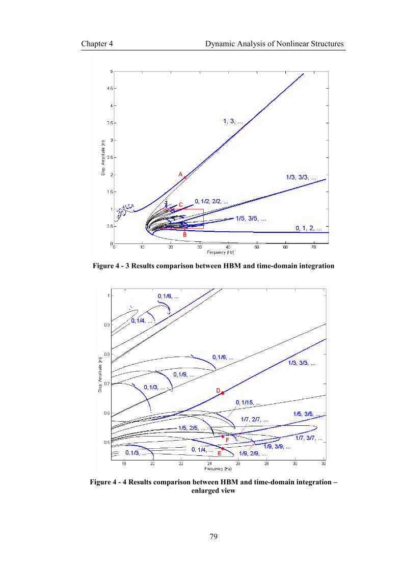
Chapter 4 Dynamic Analysis of Nonlinear Structures
79
Figure 4 - 3 Results comparison between HBM and time-domain integration
Figure 4 - 4 Results comparison between HBM and time-domain integration –
enlarged view
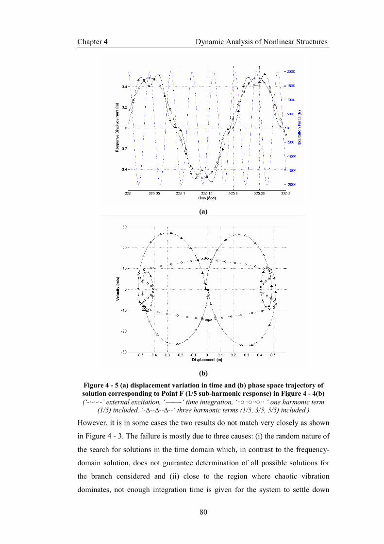
Chapter 4 Dynamic Analysis of Nonlinear Structures
80
(a)
(b)
Figure 4 - 5 (a) displacement variation in time and (b) phase space trajectory of
solution corresponding to Point F (1/5 sub-harmonic response) in Figure 4 - 4(b)
(‘-·-·-·-’ external excitation, ‘-‘ time integration, ‘········ ‘ one harmonic term
(1/5) included, ‘-∆--∆--∆--‘ three harmonic terms (1/5, 3/5, 5/5) included.)
However, it is in some cases the two results do not match very closely as shown
in Figure 4 - 3. The failure is mostly due to three causes: (i) the random nature of
the search for solutions in the time domain which, in contrast to the frequency-
domain solution, does not guarantee determination of all possible solutions for
the branch considered and (ii) close to the region where chaotic vibration
dominates, not enough integration time is given for the system to settle down
Chapter 4 Dynamic Analysis of Nonlinear Structures
81
and (iii) the time-domain solution approach allows us to find only stable steady-
state solutions and misses unstable ones.
There are several more interesting discoveries from this exercise, which is
somewhat off the main thread of this thesis. More details are shown in Appendix
B.
4.5 Concluding Remarks
This chapter focuses on the dynamic analysis of nonlinear structures, and in
particular on the periodic response due to external periodic excitation. Nonlinear
differential equations that describe the dynamic system can rarely be solved
analytically, as concluded by many mathematicians. The approximation methods
are good alternatives. Some of them have been presented in this chapter. It is
demonstrated in the Case Study that the Harmonic Balance Method is accurate
and efficient in solving a problem with strong nonlinearity. A large number of
steady-state solutions co-exist at the same excitation frequency and the
Harmonic Balance Method is capable of finding them.

Chapter 5 Nonlinear Structural Coupling
82
Chapter 5
Nonlinear Structural Coupling
5.1 Introduction
Structural coupling methods originated from the demand for efficient analysis of
complex structures during a time when high performance computers were still
rare. The problem of modelling a complicated structure could be greatly
simplified by first dividing the structure into components, each of which could
be represented by a smaller, more accurate and refined mathematical model; and
then applying some coupling schemes to analyse the dynamic response of the
whole assembly from the dynamic properties of individual components [13]. In
addition to the savings made in computation time, the concept of structural
coupling allows component models to be generated from different sources. It is
common in practice that certain component models are better derived from
experiment, and the others from direct FE construction. The accuracy and
completeness of the assembly model, as well as the dynamic responses obtained,
will benefit from optimal component model description.
The linear structural coupling methods are well developed, as discussed in
Chapter Two. From an engineering viewpoint [12], there is a need to extend
linear coupling methods to nonlinear systems because some engineering
Chapter 5 Nonlinear Structural Coupling
83
structures are formed by largely linear components with a small number of
localised nonlinearities. Thus, a few nonlinear elements cause the whole
structural assembly to behave nonlinearly. For example, in a turbine engine, the
linear turbine blades are prevented from reaching excessive vibration levels by
using the so-called “friction dampers” at the roots connecting to the rotor. The
existence of friction dampers makes the linear calculation invalid. Another
example can be found in the dynamics of a rotor supported on nonlinear bearings,
e.g. squeeze-film bearings or active magnetic bearings. The vibration
phenomena of the rotor in this case cannot be described accurately with linear
models. In the above two examples, although the overall nonlinear behaviour is
significant, the actual number of nonlinear elements is very small. For such cases,
there is a need to develop analysis procedures whereby the linear and nonlinear
parts can be analysed separately, and combined together with some nonlinear
coupling procedures, thus avoiding a nonlinear analysis for the whole structure
[12]. It is expected that computation time will be largely reduced by such an
approach.
In the literature, the researches carried out to study the dynamic properties of
nonlinear structures mostly focused on simple or simplified structures and did
not differentiate the extent of nonlinearity in the structure, be it local or global.
For time domain analysis, the combination of nonlinearity and large model size
causes numerical integration to be impractical, except perhaps for short time
transient response calculation. For frequency-domain analysis, even though it is
much more efficient than time-domain analysis in finding steady-state solutions,
once the model size gets large the iterations can get slower and numerically more
unstable. If we can combine frequency-domain methods together with the
concept of structural coupling, it is possible to analyse large size structures with
localised nonlinearities effectively.
In this chapter, nonlinear structural coupling methods are reviewed and the focus
is on frequency domain methods with the FRF coupling approach. Vibration
caused by periodic excitation is of major concern in many practical cases; hence
a test rig model under periodic external excitation is used to assess the nonlinear
coupling method. Different nonlinearities are assigned to the model in order to
show the versatility and efficiency of the method.

Chapter 5 Nonlinear Structural Coupling
84
5.2 Nonlinear Structural Coupling Approaches
There is not much literature available on this topic, even though it is apparently a
subject worth more attention. The fundamental idea is to separate the linear and
nonlinear part of the assembly. The first stage is the sub-structuring of the
original nonlinear system into subsystems, or components, that can be modelled
separately: This step achieves two objectives [67]:
• it results in the division of a larger system into smaller subsystems which may
be easier to model or to identify from experimental data, and
• it enables the segregation of linear and nonlinear components which will
eventually result in an economical analysis procedure.
One of the earliest attempts was made by Dowell [68], who used the Component
Mode Synthesis method with Lagrange multiplier to analyse a simply supported
beam attached to a nonlinear spring-mass system. Nataraj et al. [67] also used
Component Mode Synthesis method and, together with trigonometric collocation
method, to calculate periodic solutions of a rotor system with nonlinear support.
Watanabe and Sato [69] proposed the so-called Nonlinear Building Block
approach to evaluate frequency response characteristics of a structural system
with nonlinear springs linking linear components. They used the spatial coupling
method and represented the join nonlinearity with its describing function. The
use of Guyan reduction [18] on the linear components before applying nonlinear
algorithms to calculate the response of the whole assembly has also been tried
[70]. The Frequency Response Function (FRF) coupling method has also been
explored to obtain steady state periodic response of structural assemblies with
localised nonlinearity. This approach is, however, not widely seen in the
literature. To the author’s knowledge only Petrov [64] and Ferreira [13] have
touched on this topic. Ferreira’s approach is a direct extension of the linear FRF
coupling method, with an additional nonlinear joint matrix added to the
assembly FRF matrix. This additional joint matrix is derived using the
describing function method. Petrov’s approach uses the Harmonic Balance
Method and takes the advantage of the fact that omitting internal linear DOFs
will not affect the accuracy and completeness of the calculated response if the
component models are represented with FRF matrices, and the resultant

Chapter 5 Nonlinear Structural Coupling
85
assembly model is also in the form of FRF matrix. Iteration is required in both
approaches and the Newton-Raphson method is preferred.
5.2.1 Nonlinear FRF Coupling With Describing Function Method
This method was first suggested by Ferreira et. al [13, 71]. It combines the well-
developed linear FRF method with linearised description of the nonlinear joints
using describing function method. There are different forms of FRF coupling
formations, the most basic one has been briefly presented in Chapter Two. A
slightly more detailed version is presented below. Two components A and B are
modelled and represented with their respective FRF matrices:
( ) ( )
U H F
U H F
A A A
B B B
ω
ω
=
= (5.1)
Each matrix is arranged according to the locations of the DOFs:
U H H F
U H H F
U H H F
U H H F
A i A ii A ic A i
A c A ci A cc A c
B i B ii B ic B i
B c B ci B cc B c
=
=
(5.2)
The subscripts i and c represent the internal and connecting DOFs, respectively.
It is assumed that components A and B are connected rigidly at the interface. By
applying the equilibrium and compatibility equations at the interface:
F F F
U U U
A c B c c
A c B c c
= − =
= = (5.3)
the combined system FRF matrix can be derived and represented as:
( ) ( ) ( )1
1 1
1
C A A
A ii A ic
A ci A cc B cc B ci
B ic B ii
ω ω ω−− −
−
= ⊕
= +
H H H
Z Z 0
Z Z Z Z
0 Z Z
(5.4)
In which [ ]Z is the dynamic stiffness matrix, and derived from the inversion of
the FRF matrix as:
Chapter 5 Nonlinear Structural Coupling
86
( ) ( )1
Z Hω ω−
= (5.5)
The system equation is therefore expressed as:
1
A i A ii A ic C i
c A ci A cc B cc B ci c
B i B ic B ii C i
− = +
U Z Z 0 F
U Z Z Z Z F
U 0 Z Z F
(5.6)
and in a compact form:
( ) U H FC C Cω = (5.7)
The main advantage of the FRF coupling method is that FRFs measured from
experiments can be used directly, which means within the frequency range of
interest there is no approximation made throughout the derivation of the system
FRF matrix. In addition, the assembly model size can be reduced without
sacrificing accuracy by including only the connecting DOFs and internal DOFs
of interest in the component matrices. The reason is that FRFs derived at any
DOF record the dynamic information of the whole structure. Hence, even with
the physical DOFs omitted from the FRF matrix, the resultant FRF matrix still
truly represents the component. This can significantly reduce the size of the
problem since the connecting DOFs normally form only a small portion of the
whole structure.
As shown in equation (5.4), three matrix inversions are required to derive the
system FRF matrix. This hinders a wider application of this method because of
excessive computing time needed and possible ill-conditioned matrices near
resonance causing erroneous results [16]. An alternative FRF coupling method
introduced by Jetmundsen et al. [14] reduces the number of matrix inversions at
each frequency point from three to one. In addition, the size of the matrix to be
inverted is restricted to the connecting DOFs only. This further reduces the
calculation requirement. The resultant assembly RFR matrix is expressed as:
( ) [ ] 1
H H 0 H H
H H H 0 H H H H
0 0 H H H
T
A ii A ic A ic A ci
C A ci A cc A cc A cc B cc A cc
B ii B ic B ci
ω−
= − + − −
(5.8)
Chapter 5 Nonlinear Structural Coupling
87
Using the same structural coupling concept as described above, Ferreira [13]
considered the flexibilities between the connecting DOFs and modelled them
with an additional matrix, which, in the presence of nonlinearity, is deduced
with describing function method. The derivation starts from defining separately
the pre- and post- coupling matrices as:
U H H H F
U H H H F
U H H H F
i ii ip iq i
p pi pp pq p
q qi qp qq q
=
(5.9)
And
U H H H F
U H H H F
U H H H F
I II IP IQ I
P PI PP PQ P
Q QI QP QQ Q
=
(5.10)
Here the lower-case subscripts represent the matrices obtained in the pre-
coupling condition, and the upper-case subscripts the post-coupling condition,
which are to be determined from some mathematical manipulations. All the
internal DOFs are grouped together as Ui and U I , and the connecting DOFs
from the two joining components are expressed as U p , UP and Uq , UQ . The
existence of the flexible joint poses different boundary compatibility and
equilibrium conditions, and the joint is expressed as:
[ ]F U U
F U U
p pp pq p p
q qp qq q q
− = =
G GG
G G (5.11)
Each entry of the matrix [ ]G is a main-harmonic describing function for the
joint impedance of a connecting pair. The describing function is a quasi-linear
representation for a nonlinear element subjected to sinusoidal excitation. The
resultant system equation, including the effect of nonlinear joint, is expressed as:
[ ] 1
U H H H H H H H F
U H H H H H B H H F
U H H H H H H H F
T
I ii ip iq ip iq ip iq I
P pi pp pq pp pq pp pq P
Q qi qp qq qp qq qp qq Q
−
− −
= − − − − −
(5.12)
in which

Chapter 5 Nonlinear Structural Coupling
88
-1
B H H H Hpp qq pq qp= + − − +G (5.13)
Each describing function is a function of relative displacements between the
connection coordinates; therefore equation (5.12) is a system of nonlinear
algebraic equations to be solved iteratively at each frequency point of interest.
The above derivation shows how two component models can be ‘joined’
mathematically. The same concept can be extended to ‘join’ more than two
component models at one time. This can be achieved by re-arranging the FRF
matrix. Additionally, multi-harmonic terms can be included in the describing
functions [13, 72]. They will nevertheless multiply the order of the problem, and
make this method non-economical.
5.2.3 Nonlinear FRF Coupling with Harmonic Balance Method
For a structural assembly with the equation of motion:
[ ] [ ] [ ] ( ) ( ) ( ) ( ) ( ), ( )M u C u K u + g u u ft t t t t+ + =ɺɺ ɺ ɺ (5.14)
the response, excitation and nonlinear internal force are expressed in complex
multi-harmonic terms:
( ) ( ) ( )
0
1
1
1
0
1
0
1
,
2
u U U
u U
u U
g u u G U G U
f F F
nN i tn m
m m m
n
nN i tn m
m m
n
nN i tn m
m m
n
nN i tn m
m m m m
n
nN i tn m
m m m
n
e
ni e
m
ne
m
e
e
ω
ω
ω
ω
ω
ω
ω
=
=
=
=
=
= +
=
= −
= +
= +
∑
∑
∑
∑
∑
ɺ
ɺɺ
ɺ
(5.15)
in which ω is the frequency of the external harmonic forcing, and m is an
integer corresponding to the ratio of the period of the external forcing to the
period of the response. It is used to count for sub-harmonic responses; m=1
when the dominant harmonic in the response is the same as that of the excitation;
Un
m is the amplitude of the nth
complex harmonic term; N is the total number of
harmonic terms included in the Fourier series expansions.
Chapter 5 Nonlinear Structural Coupling
89
Substitute (5.15) into (5.14) and balance each harmonic term. The subscript m is
dropped for clarity.
( ) ( ) ( )
( ) ( ) ( )
( ) ( ) ( )
( ) ( ) ( )
0 0 0 0 0
0
1 1 1 1 1 11 12
2
2
KU G U Z U G U F
K M+ C U G U Z U G U F
K M+ C U G U Z U G U F
K M+ C U G U Z U G U F
n n n n n n
N N N N N N
im m
n ni
m m
N Ni
m m
ω
ω ω ω
ω ω ω
ω ω ω
+ = + =
− + = + =
− + = + =
− + = + =
⋮
⋮
(5.16)
Combine all these equations into a compact equation:
( ) ( ) ( )- 0R U Z U F+G Uω= = (5.17)
Where 0 1, , , , ,T
n NU= U U U U⋯ ⋯ is a vector of harmonic coefficients of the
response at all system DOFs; 0 1, , , , ,F F F F FT
n N= ⋯ ⋯ is a vector of harmonic
coefficients of the external excitation force; ( ) 0 1, , , , ,G U G G G GT
n N= ⋯ ⋯ is
a vector of harmonic coefficients for all the nonlinear internal forces; ( )Z ω is
the dynamic stiffness matrix of the linear part of the system, composed of all
harmonic components as:
( )
2
2
2
1 1
K 0 0 0 0
0 K M+ C 0 0 0
0 0 0 0
ZK M+ C
0 0 0 0
0 0 0 0 K M+ C
im m
n ni
m m
N Ni
m m
ω ω
ωω ω
ω ω
− = − −
⋯
⋯
⋱ ⋯
⋮ ⋮ ⋮ ⋮ ⋮
⋯ ⋱
⋯
(5.18)
This is very similar to equation (4.32), only that this time the entries are in
complex form and the size of the matrix is half the original. Multiply (5.17) with

Chapter 5 Nonlinear Structural Coupling
90
the FRF matrix of the uncoupled assembly, including all the harmonic terms of
interest, and we will have:
( ) ( ) ( )- ] 0R U U H [F G Uω= − = (5.19)
in which:
( )
[ ] 1
12
12
12
1 1
K 0 0 0 0
0 K M+ C 0 0 0
0 0 0 0
HK M+ C
0 0 0 0
0 0 0 0 K M+ C
im m
n ni
m m
N Ni
m m
ω ω
ωω ω
ω ω
−
−
−
−
−
= − −
⋯
⋯
⋱ ⋯
⋮ ⋮ ⋮ ⋮ ⋮
⋯ ⋱
⋯
(5.20)
This equation can be solved with the Newton-Raphson iteration method, which
has quadratic convergence when an initial approximation is close enough to the
exact solution. The attractive bit of this equation is that the FRF matrix, ( )H ω ,
can be readily formed either from direct experimental measurement or from FE
modal calculations of the linear combination of the whole assembly. For the nth
harmonic term in the FRF matrix:
( )( )
21 21
ψ ψH
mNn r r
r
r r
ni
m
ω
η ω ω
∗
=
= − −
∑ (5.21)
In which, Nm is the number of modes that are used in the modal expansion;
rω and ψ r are the corresponding rth
natural frequency and mode shape. In many
cases, a small number of modes kept in the modal expansion will provide
sufficient accuracy in the formation of the FRF matrix.
The use of the FRF matrix to describe the assembly system allows all DOFs
where only linear internal interaction forces are applied to be excluded without
any loss of accuracy and completeness of the model [64]. The resultant equation
only includes DOFs where nonlinear internal interaction forces and external
excitation forces are applied, and where the responses are of concern. This will
Chapter 5 Nonlinear Structural Coupling
91
considerably reduce the size of the equations and the computational cost
accordingly.
In order to exclude those linear DOFs, equation (5.19) can be re-written in a
form in which the displacement vector of a particular harmonic term Un is
partitioned into a vector consisting discarded linear DOFs lin_dUn , retained linear
DOFs lin_rUn and nonlinear DOFs nlnU
n .
( ) ( )lin_d lin_d lin_d
lin_r lin_r lin_r
nln nln nln
-
U F G
R U U H F G
U F G
n n n
n n n n n
n n n
ω
= −
(5.22)
With the fact that lin_dFn =0 and lin_dG
n =0, this equation is reduced to:
( ) ( )lin_r lin_r lin_r
red red
nln nln nln
-U F G
R U HU F G
n n n
n n
n n nω
= −
(5.23)
or, in a more compact form:
( ) ( )red red red red red-R U U H F Gn n n n nω = − (5.24)
and with all the harmonics included, equation (5.19) is reduced to:
( ) ( ) ( )red red red red red red- 0R U U H F G Uω = − = (5.25)
Equation (5.25) can be solved numerically with the Newton-Raphson method
detailed in section 4.3.3.
5.3 Case Studies
In this section, a representative aero-engine test rig model is studied. This single-
rotor test rig has one of its two bearing supports specially designed to exhibit
considerable nonlinearity, and this results in the whole assembly being studied
with nonlinear approaches. The linear parts of the test rig are all flexible; hence
adequately detailed FE models are needed to capture even localised flexibilities.
This nevertheless leads to large order system equations to be solved.
In the field of structural dynamics involving rotating components, mostly
encountered in the literature are those analyses based on simplified models,
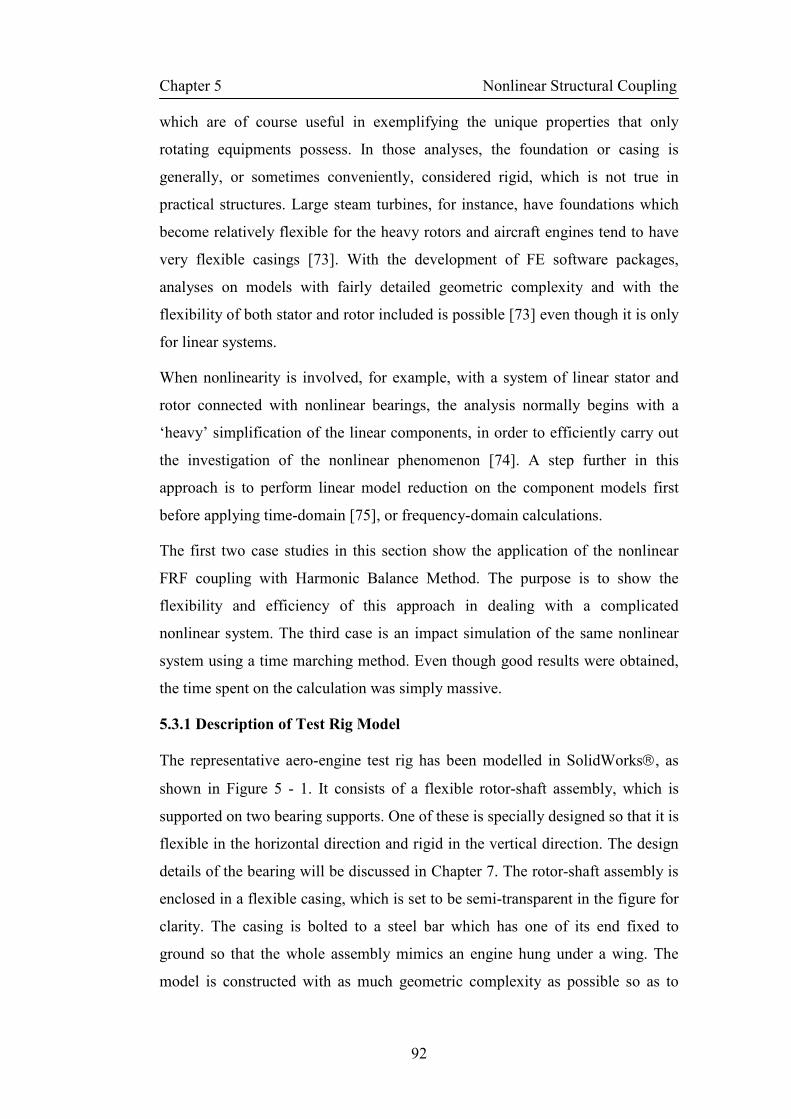
Chapter 5 Nonlinear Structural Coupling
92
which are of course useful in exemplifying the unique properties that only
rotating equipments possess. In those analyses, the foundation or casing is
generally, or sometimes conveniently, considered rigid, which is not true in
practical structures. Large steam turbines, for instance, have foundations which
become relatively flexible for the heavy rotors and aircraft engines tend to have
very flexible casings [73]. With the development of FE software packages,
analyses on models with fairly detailed geometric complexity and with the
flexibility of both stator and rotor included is possible [73] even though it is only
for linear systems.
When nonlinearity is involved, for example, with a system of linear stator and
rotor connected with nonlinear bearings, the analysis normally begins with a
‘heavy’ simplification of the linear components, in order to efficiently carry out
the investigation of the nonlinear phenomenon [74]. A step further in this
approach is to perform linear model reduction on the component models first
before applying time-domain [75], or frequency-domain calculations.
The first two case studies in this section show the application of the nonlinear
FRF coupling with Harmonic Balance Method. The purpose is to show the
flexibility and efficiency of this approach in dealing with a complicated
nonlinear system. The third case is an impact simulation of the same nonlinear
system using a time marching method. Even though good results were obtained,
the time spent on the calculation was simply massive.
5.3.1 Description of Test Rig Model
The representative aero-engine test rig has been modelled in SolidWorks, as
shown in Figure 5 - 1. It consists of a flexible rotor-shaft assembly, which is
supported on two bearing supports. One of these is specially designed so that it is
flexible in the horizontal direction and rigid in the vertical direction. The design
details of the bearing will be discussed in Chapter 7. The rotor-shaft assembly is
enclosed in a flexible casing, which is set to be semi-transparent in the figure for
clarity. The casing is bolted to a steel bar which has one of its end fixed to
ground so that the whole assembly mimics an engine hung under a wing. The
model is constructed with as much geometric complexity as possible so as to

Chapter 5 Nonlinear Structural Coupling
93
represent a real structure more accurately. The exact dimensions of each
component can be found in Appendix A.
Figure 5 - 1 A schematic view of the test rig in Solidworks
The 3-D solid model of the test rig was exported to ANSYS, and the resultant
FE model is shown in Figure 5 - 2, in which (b) is a cross-sectional view.
Besides the two vertical strips attached to the front bearing block, which are
displayed in purple, the bulk structure is formed with element Solid451. The two
vertical strips are formed with Shell632. There are a total of 24065 elements and
46055 nodes, which comprise 138165 DOFs when the full system equation is
formed. This is of course not comparable to the scale of industrial engine models;
nevertheless, such a size of FE model has not been seen applied with various
nonlinear methodologies in literature.
(a) (b)
Figure 5 - 2 FE model of the test rig
1 Solid45 is a 3-D structural solid element in ANSYS. This element is defined by eight nodes having three translational degrees of freedom at each node. 2 Shell63 is a 3-D structural Elastic Shell element in ANSYS. This element is defined by 4 nodes having three translational and three rotational degrees of freedom at each node.
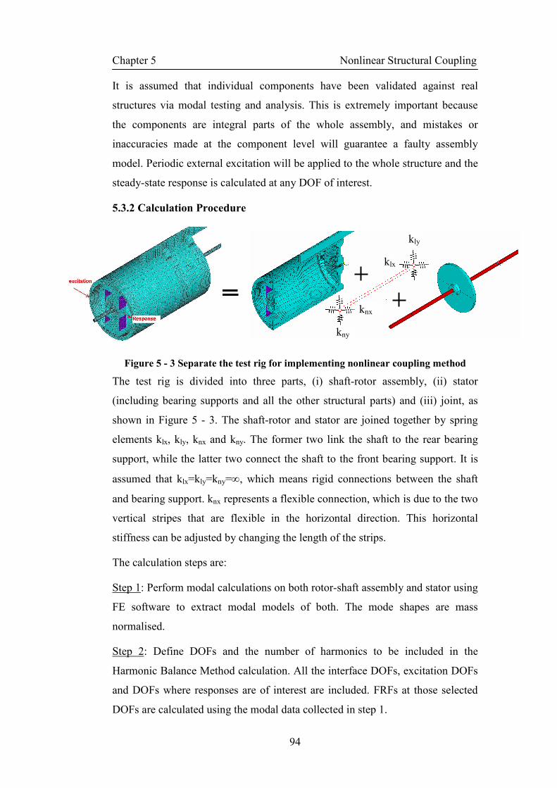
Chapter 5 Nonlinear Structural Coupling
94
It is assumed that individual components have been validated against real
structures via modal testing and analysis. This is extremely important because
the components are integral parts of the whole assembly, and mistakes or
inaccuracies made at the component level will guarantee a faulty assembly
model. Periodic external excitation will be applied to the whole structure and the
steady-state response is calculated at any DOF of interest.
5.3.2 Calculation Procedure
Figure 5 - 3 Separate the test rig for implementing nonlinear coupling method
The test rig is divided into three parts, (i) shaft-rotor assembly, (ii) stator
(including bearing supports and all the other structural parts) and (iii) joint, as
shown in Figure 5 - 3. The shaft-rotor and stator are joined together by spring
elements klx, kly, knx and kny. The former two link the shaft to the rear bearing
support, while the latter two connect the shaft to the front bearing support. It is
assumed that klx=kly=kny=∞, which means rigid connections between the shaft
and bearing support. knx represents a flexible connection, which is due to the two
vertical stripes that are flexible in the horizontal direction. This horizontal
stiffness can be adjusted by changing the length of the strips.
The calculation steps are:
Step 1: Perform modal calculations on both rotor-shaft assembly and stator using
FE software to extract modal models of both. The mode shapes are mass
normalised.
Step 2: Define DOFs and the number of harmonics to be included in the
Harmonic Balance Method calculation. All the interface DOFs, excitation DOFs
and DOFs where responses are of interest are included. FRFs at those selected
DOFs are calculated using the modal data collected in step 1.
kly
klx
knx
kny

Chapter 5 Nonlinear Structural Coupling
95
Step 3: Define joint parameters. This also includes providing information of
DOF pairs where the connection is made. Both damping and stiffness are used to
quantify the joint properties.
Step 4: Apply Harmonic Balance Method with FRF coupling. An internally
developed code FORSE [66] is used.
5.3.3 Results
When the two vertical strips are slightly compressed, buckling occurs. The
stiffness knx displays properties as plotted in Figure 5 - 4, which is from a real
experiment measurement. O is the global centre, which is an unstable
equilibrium point. A and B are two stable local equilibrium points.
-4 -3 -2 -1 0 1 2 3 4-60
-40
-20
0
20
40
60
mm
N
A B O
Figure 5 - 4 Force and displacement relation of the stiffness knx
5.3.3.1 Case one – joint with weakening stiffness property
Small periodic excitation force is used in this case. The excitation and response
nodes and directions are shown in Figure 5 - 3. It is expected that the DOFs
connected with spring knx vibrate locally around either point A or B along the
stiffness property line as shown in Figure 5 - 4. This is indeed a case of
weakening stiffness. The resultant Frequency Response Function plot is shown
in Figure 5 - 5. Four calculation runs were carried out, using different excitation
force levels as marked in the drawing. The mode at 27Hz is prominently affected
by the joint nonlinearity. The FRF curves bend towards lower frequency as the
excitation force increases. This manifests a weakening stiffness. Figure 5 - 6
shows a closer look of the FRF curves nearby 27Hz. The mode at 75Hz is not
affected by the nonlinearity. It is observed in the FE simulation that this is the

Chapter 5 Nonlinear Structural Coupling
96
second bending mode of the whole test rig in the horizontal direction, which is
not influenced by the nonlinear stiffness we have set.
20 30 40 50 60 70 80 90 10010
-3
10-2
10-1
100
101
Frequency (Hz)
FRF Amplitude (m/s2/N)
4N
3N2N
1N
Figure 5 - 5 Frequency response function curves based on Harmonic Balance
Method calculation for a system with joint of weakening stiffness property
18 20 22 24 26 28 30
100
Frequency (Hz)
FRF Amplitude (m/s2/N)
4N
3N
2N
1N
Figure 5 - 6 A close look of the frequency response function curves nearby 27.5Hz
5.3.3.2 Case two – joint with polynomial stiffness property
Large periodic excitation force is used in this case. The excitation and response
nodes and directions are shown in Figure 5 - 3. It is expected that the DOFs
connected with spring knx vibrate globally around point O along the stiffness
property line in Figure 5 - 4.
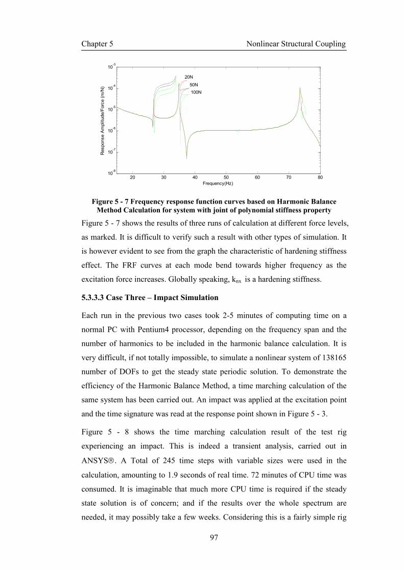
Chapter 5 Nonlinear Structural Coupling
97
20 30 40 50 60 70 8010
-8
10-7
10-6
10-5
10-4
10-3
Frequency(Hz)
Response Amplitude/Force (m/N)
20N
50N
100N
Figure 5 - 7 Frequency response function curves based on Harmonic Balance
Method Calculation for system with joint of polynomial stiffness property
Figure 5 - 7 shows the results of three runs of calculation at different force levels,
as marked. It is difficult to verify such a result with other types of simulation. It
is however evident to see from the graph the characteristic of hardening stiffness
effect. The FRF curves at each mode bend towards higher frequency as the
excitation force increases. Globally speaking, knx is a hardening stiffness.
5.3.3.3 Case Three – Impact Simulation
Each run in the previous two cases took 2-5 minutes of computing time on a
normal PC with Pentium4 processor, depending on the frequency span and the
number of harmonics to be included in the harmonic balance calculation. It is
very difficult, if not totally impossible, to simulate a nonlinear system of 138165
number of DOFs to get the steady state periodic solution. To demonstrate the
efficiency of the Harmonic Balance Method, a time marching calculation of the
same system has been carried out. An impact was applied at the excitation point
and the time signature was read at the response point shown in Figure 5 - 3.
Figure 5 - 8 shows the time marching calculation result of the test rig
experiencing an impact. This is indeed a transient analysis, carried out in
ANSYS. A Total of 245 time steps with variable sizes were used in the
calculation, amounting to 1.9 seconds of real time. 72 minutes of CPU time was
consumed. It is imaginable that much more CPU time is required if the steady
state solution is of concern; and if the results over the whole spectrum are
needed, it may possibly take a few weeks. Considering this is a fairly simple rig

Chapter 5 Nonlinear Structural Coupling
98
model comparing to the industrial ones, it apparently shows the advantage of the
Harmonic Balance Method in cutting down the calculation time for such a
nonlinear system.
0 0.2 0.4 0.6 0.8 1 1.2 1.4 1.6 1.8-15
-10
-5
0
5
10
15
20
25
30
Time (Sec)
Acceleration (m/s2)
Figure 5 - 8 Time marching calculation result
This impact simulation result has actually been compared with an impact test
[76]. It showed good agreement as demonstrated in the following plot, in which
the red line is the experimental measurement data.
Figure 5 - 9 Time marching calculation result comparison
-0.5 0 0.5 1 1.5 2 -15
-10
-5
0
5
10
15
20
25
30
Time (Sec)
Acceleration (m/s
2)
Chapter 5 Nonlinear Structural Coupling
99
5.4 Concluding Remarks
Examples in the above case study shows how efficient the FRF coupling with
Harmonic Balance Method is in dealing with a large scale structural assembly
with localised nonlinearity. It takes no more than a few minutes to find steady
state solutions across the spectrum. If a conventional time domain method is
used, it will take hours of CPU time just to calculate a transient response for
such a system.
There are other nonlinear structural coupling methods available and were
discussed in this chapter. In general, they are using linear coupling methods to
firstly reduce the size of the problem and then apply different nonlinear methods
on the reduced model. The accuracy of the response calculation for the assembly
depends on how well the linear model is reduced, which normally has some
approximation implied in the process. FRF coupling method, on the other hand,
is an exact method, which is of course preferred if it can be integrated with
certain nonlinear methods.

Chapter 6 Structural Dynamic Testing and FRF Measurement Techniques
100
Chapter 6
Structural Dynamic Testing and FRF
Measurement Techniques
6.1 Introduction
Structural dynamic testing is a very broad topic. Depending on its purpose, there
are two types of dynamic test we normally encounter. The first type involves the
test structure being subjected to a real or simulated environment in which it
operates. By doing so, we can assess the test structure’s dynamic behaviour
under working conditions. This type of test is also called an operational test,
which is especially widely used when a product is at its final design stages.
Information, such as how or whether it will survive extreme working conditions,
or whether its performance satisfies the design criterion, is collected. This type
of test normally only requires the measurement of the response level to
understand the behaviour of the test structure. The second type of dynamic test is
meant to establish more detailed knowledge of the structure by linking the
excitation and response. By doing so, it is possible to build a mathematical
model to represent the structure. The same type of mathematic model can also be
derived from theoretical analysis, mainly with the help of Finite Element based
software. Hence, we can link design with test, aiming to update and validate the
FE models, and to make design modifications more predictable. This type of test

Chapter 6 Structural Dynamic Testing and FRF Measurement Techniques
101
is widely known as Modal Testing, in which measuring the Frequency Response
Functions and extracting the modal properties are the main objectives. This
chapter focuses on modal testing and its extension into nonlinear territory, in
which the relation between the response and excitation are still sought after.
With the advancement of computing technology and the Finite Element methods,
it is suggested that tests can be substituted with simulations of computer-
generated mathematical models. It is never unreasonable to imagine so, but at
the moment dynamic testing is not replaceable, simply because:
• Some important physical parameters still cannot be modelled correctly due to
our limited understanding, e.g. friction, which sometimes has a big influence
on the dynamic behaviour of the whole structure;
• Even if it is possible to model the structure correctly, variability between
products of the same design will induce different dynamic behaviour;
• Not all working conditions can be simulated. Either it is too complicated to
describe or simply not economical to be put into calculation;
• Human error during the modelling stage are difficult to discover;
• Last but not least, in the process of developing and validating new simulation
algorithms, comparison with test results of a physical item is essential.
Being able to understand the necessity of a dynamic test helps to appreciate the
importance of good test practice. A physical test is just like a mathematical
modelling and simulation job. It involves a chain of operations, mistakes at any
one of which will cause errors in the results. This is particularly dangerous
because people tend to have more confidence in the test results than in computer
simulated ones and trust more what they can observe physically. Therefore, a
deep understanding of the test itself is very important: from test setup to data
processing, from test structure preparation to catering for physical limitations of
test system.
In this chapter, the basic measurement chain in Modal Testing is introduced first,
and is followed by detailed descriptions of test equipment used in those tests
involved in this thesis work. FRF measurement techniques are presented
afterwards. They are grouped according to different types of excitation signals
used, with the understanding that FRF derivation varies depending on the signal

Chapter 6 Structural Dynamic Testing and FRF Measurement Techniques
102
form. The advantages and disadvantages of each type of signal are also discussed.
This leads to the discussion of FRF measurement on nonlinear structures.
Special treatment is required to identify nonlinearity in a structure, or to validate
predictions from nonlinear calculation algorithms. The amplitude of either
excitation or response must be controlled. An algorithm is presented
mathematically on how it is done. This algorithm has been implemented in a
LabVIEW-based code.
It should be noted that dynamic testing can be a topic of a whole book [77, 78].
It is not the author’s intention to display here every bit of it, rather, only those
relevant to this thesis work are touched upon.
6.2 Basic Measurement Chain
We expect to obtain the dynamic properties of a structure, in terms of natural
frequencies, damping ratios and mode shapes, by conducting dynamic tests.
Those properties can be deduced from the Frequency Response Function, which
is obtained by taking the ratio between the response and excitation in the
frequency domain; hence it is natural to design an experiment that enables both
excitation and response to be measured simultaneously.
Figure 6 - 10 Schematic representation of basic measurement chain for modal testing
Figure 6 - 10 shows a typical experimental setup used for FRF measurement.
There are many variations in terms of the exact hardware used and the way data
processed. Nevertheless, all the setups consist the following major items [1]:
• Excitation system: Signal Generator, Power Amplifier, Shaker, Impact
Hammer, etc;
• Sensing system: Transducers, Conditioning Amplifier, etc;
Signal
Generator Shaker
Conditioning
Amplifier
Power
Amplifier
Analyser
Test Structure
CONTROLLER
Force
Transducer
Response
Transducer
Chapter 6 Structural Dynamic Testing and FRF Measurement Techniques
103
• Analysing System: FFT Analyser, etc.
The various tests conducted within this thesis used the above basic measurement
chain. The excitation to the test structure is provided by the shaker, which
generates a motion following the pattern of the electric current signal it receives
from the power amplifier. The excitation signal originates from the signal
generator, which is capable of creating a variety of different signals to match the
requirements of the structure under test, but it is usually sinusoidal. When an
Impact Hammer is used as the excitation device, Signal Generator and Power
Amplifier will not be used. The sensing system converts mechanical signals, e.g.
force and acceleration, into electronic signals, which are easier to handle. After
both excitation and response signals are collected and fed into the analyzer, in
the form of time-domain analogue signals, the analyser converts them into
frequency domain, and computes the Frequency Response Function hereafter.
It is a common practice nowadays that the signal generator and the analyser are
combined into a single unit, which not only makes the test setup more compact,
but also improves the controllability of the test itself. Controlled-level dynamic
testing, which will be discussed in detail in later sections, is made possible by
linking the output from the analyser to the creation of excitation signal from the
signal generator; and this is easily accomplished in a single controller unit.
The test structure is also an integral part of the experimental setup. It influences
the selection of hardware and excitation type to be used in order to maximise the
data quality in a most economical way. The treatment of the test structure can
affect the test results prominently. Topics that concern, for example, boundary
conditions and optimised location of transducers, are themselves worth in-depth
research effort.
6.3 Excitation and Measurement System
This section focuses on individual hardware used in various modal tests
conducted within the scope of this thesis. Sound knowledge of the hardware’s
functionalities is the first step towards achieving reliable test results.
Chapter 6 Structural Dynamic Testing and FRF Measurement Techniques
104
6.3.1 Excitation
The purpose of having an excitation source is to inject kinetic energy into the
test structure, and by observing the behaviour of the structure, we can quantify
its inherited dynamic properties. Many different types of excitation schemes are
employed in vibration testing. Some examples are [77]: a sudden release of a
static load; an impact force; mechanical exciter based on either direct-drive or
rotating unbalance; electrohydraulic exciter and the most popular one:
electromagnetic exciter, commonly known as a shaker. This section elaborates
on the two excitation methods used in this thesis’ experimental work. One is
with the application of an impact hammer, and one with a shaker.
Vibration tests with the application of an impact hammer have some advantages
that allow it to be used widely in structural dynamic testing. Firstly, the test
setup is simple. The equipment consists of no more than a hammer with a set of
different tips, which allow the excitation frequency range to be varied for
different test structures. Secondly, hammer test is the fastest method when a
preliminary result is needed. Thirdly, it is a much more economical tool
comparing to shakers. Nevertheless, the impact hammer has shortcomings that
make the use of the other types of exciter is a must in some cases. Firstly, it is an
open-loop test. The applied force level is not controlled. This limits its
application to linear test only. Secondly, the frequency range that the test
structure can be excited is limited and restricted to the type of impact header
used. It may possibly happen that some important vibration modes cannot be
captured. Thirdly, though the test setup is simple, the requirement for the
operator is actually quite high. He/she has to select the right types of impact tip,
apply the right window functions to the signals, and be consistent in the way the
impact is applied: the point of hitting should be precise, and the impact direction
should be normal to the surface.
The electromagnetic shaker is perhaps the most common type of exciter. The
supplied input signal is converted to an alternative magnetic field in which is
placed a coil which is attached to the drive part of the device, and to the structure.
Some of its advantages are: the frequency and amplitude of excitation can be
controlled independently, giving more operational flexibility; a large frequency
range can be applied, and the variety of excitation pattern is virtually limitless,
Chapter 6 Structural Dynamic Testing and FRF Measurement Techniques
105
which solely depends on the capability of the signal generator; by linking the
analyser and the signal generator, it is possible to implement a control system to
conduct nonlinear test.
The choice of the exciter to be used depends on many factors, e.g., purpose of
the test, time constraint, accuracy requirement, and physical constraint of the test
structure. In this thesis, impact test is conducted for identifying the dynamic
properties of linear structures with simple geometry. The shaker is used in the
test to identify the nonlinearity, as well as validate the assembly algorithm. That
will be presented in Chapter 7.
6.3.2 Sensing
It is shown from the basic measurement chain that both excitation and response
of the structure need to be captured and quantified properly in order to construct
the Frequency Response Functions to extract the dynamic properties. The
mechanical response of a structure may be defined in terms of displacement,
velocity or acceleration. Any one of these parameters can be used to derive the
fundamental response function. The most commonly used response transducer is
the piezoelectric accelerometer, and indeed the most common force transducer
used is also piezo-material based.
Inside these piezoelectric transducers, piezoelectric materials, such as quartz or
man-made ceramics are stressed in a controlled fashion by the input force or
acceleration. This stress “squeezes” a quantity of electrical charge from the
piezoelectric material in direct proportion to the input stress, creating analogue
electrical output signal. Because of the high stiffness of those piezoelectric
materials, the piezoelectric transducers have very high resonant frequencies,
which enable them work very well across a large frequency range.
The electric charge released by the piezoelectric element is measured in the unit
of picocoulomb. It is necessary to utilise amplifiers to couple information,
contained within the tiny amount of electric charge, to the physical parameters
without dissipating it or otherwise changing it. The output from the amplifier is a
voltage signal, which is proportional to the electric charge, and in turn
proportional to either force or acceleration being measured. Bruel&Kjaer Type
2626 Condition Amplifiers were used for this purpose.

Chapter 6 Structural Dynamic Testing and FRF Measurement Techniques
106
Calibration Shaker Conditioning
Amplifier Accelerometer
Oscilloscope
Before doing any test, the transducers must be calibrated. The use of the
manufacturers’ quoted transducer sensitivities may not be accurate enough
because they can change with time and environment conditions. Both force and
motion transducers must be calibrated individually if they are to be used in a
controlled-level nonlinear test. When only linear test is involved, the calibration
can be conducted in pair, because the ratio of motion to force, not the individual
values of each parameter is used to form the Frequency Response Function.
Figure 6 - 11 shows the calibration setup for a Brüel&Kjaer Type 4393
Piezoelectric Accelerometer. A PCB portable handshaker (Model 394C06)
delivers a calibrating vibration signal at 159.2Hz with 1g RMS acceleration
output. The electric charge is amplified by the conditioning amplifier and
converted into a voltage signal, which is readable on the oscilloscope. The
sensitivity of the accelerometer is calculated by comparing the amplitude from
the readout of the oscilloscope and the calibrating signal. The resultant
sensitivity is 3.26pC/g.
Figure 6 - 11 Calibration for the accelerometer
Figure 6 - 12 shows the calibration setup for a Brüel&Kjaer Type 8200
Piezoelectric force transducer. It is a reverse process to the normal modal testing.
With the calibrated accelerometer and a solid mass of known weight, the
resultant frequency response function is a straight line according to the following
equation.
( ) 1uA
f mω = =
ɺɺ (6.1)
The shaker generates a pure tone excitation at 159.2Hz. By reading out the
acceleration and force signal in terms of voltage from the oscilloscope, and using
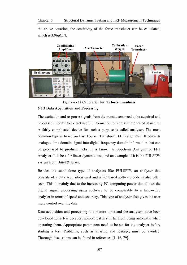
Chapter 6 Structural Dynamic Testing and FRF Measurement Techniques
107
the above equation, the sensitivity of the force transducer can be calculated,
which is 3.96pC/N.
Figure 6 - 12 Calibration for the force transducer
6.3.3 Data Acquisition and Processing
The excitation and response signals from the transducers need to be acquired and
processed in order to extract useful information to represent the tested structure.
A fairly complicated device for such a purpose is called analyser. The most
common type is based on Fast Fourier Transform (FFT) algorithm. It converts
analogue time domain signal into digital frequency domain information that can
be processed to produce FRFs. It is known as Spectrum Analyser or FFT
Analyser. It is best for linear dynamic test, and an example of it is the PULSE™
system from Brüel & Kjaer.
Besides the stand-alone type of analysers like PULSE™, an analyser that
consists of a data acquisition card and a PC based software code is also often
seen. This is mainly due to the increasing PC computing power that allows the
digital signal processing using software to be comparable to a hard-wired
analyser in terms of speed and accuracy. This type of analyser also gives the user
more control over the data.
Data acquisition and processing is a mature topic and the analysers have been
developed for a few decades; however, it is still far from being automatic when
operating them. Appropriate parameters need to be set for the analyser before
starting a test. Problems, such as aliasing and leakage, must be avoided.
Thorough discussions can be found in references [1, 16, 79].
Conditioning
Amplifiers
Oscilloscope
Accelerometer Calibration
Weight
Force
Transducer
Shaker

Chapter 6 Structural Dynamic Testing and FRF Measurement Techniques
108
6.4 FRF Measurement Techniques
The Frequency Response Function (FRF) is derived by converting time-domain
data from measurement into frequency-domain and taking the ratio of response
to excitation. Though similar hardwares are used, different calculation schemes
are employed to obtain FRFs, depending on the type of excitation signal used.
Different types of signal needs different treatment when frequency domain
information is extracted. The selection of excitation type governs the type of
transducers, digital signal processing procedures, i.e. the different FRF
measurement techniques. In this section, the categorisation is based on the
excitation signals used and we aim to choose the most suitable one according to
the applicability and other practical considerations.
6.4.1 Sine Excitation
Sine excitation test is one of the most common methods to obtain FRFs. The
commanding signal supplied to the exciter is a sinusoid with a fixed amplitude
and frequency. A prime advantage of using sine excitation is the large signal-to-
noise ratio for all the force and response measurements. This is a consequence of
the single excitation frequency for each measurement – there are no other
significant sources of excitation to contaminate the results [16]. Equally
important for this type of excitation is that the input force level to or response
level from the test structure can be accurately controlled by adjusting the
excitation signal strength at any frequency point of interest. This is crucial in the
successful evaluation of nonlinear structure due to the fact that the FRF curve in
the resonance region is distorted at a constant force level, and the resonance
frequency is shifted at different response levels.
The FRF is formed over the frequency range of interest. Therefore, the sine
excitation needs to be carried out at frequency points within the range. There are
two ways to do so. The excitation signal can be stepped from one discrete value
to another in such a way [1] as to provide the necessary density of points on the
frequency response plot. Alternatively, the excitation signal can be in the form of
a continuous sinusoid, the frequency of which is varied slowly but continuously
through the range of interest. The former method tends to be slower, but it
allows more control over the signal’s behaviour, which is crucial in nonlinear

Chapter 6 Structural Dynamic Testing and FRF Measurement Techniques
109
test. The latter is much faster, but it requires extra care on the sweep rate, a
wrong setting of which will introduce errors in the derived FRFs. Only step-sine
excitation is used in this research.
One paramount drawback of this type of excitation is the time required to obtain
an FRF is much more than other excitation methods, provided the other methods
are applicable to the same task. In sine excitation, at each frequency step,
adequate time must be allowed for the transients to die away before the force and
acceleration signals are sampled and processed. Depending on the test algorithm,
the delay can be in the form of time or number of vibration cycles or linked with
some delay-time estimation algorithm [80]. It is a trade-off sometimes when
selecting an excitation method, as which one is more important, accuracy or
efficiency. If the purpose is to validate a simulation algorithm, a more rigorous
and precise test scheme should be adopted.
6.4.2 Random Excitation
A random excitation signal is defined by a time history of random values at any
given instant. It cannot be expressed by a simple mathematical equation, like the
other types of excitation signals do, and it must be modelled probabilistically. It
is widely used in linear dynamic test because it is a fast approach to obtain
accurate estimation of a structure’s response over a broad range of frequencies.
A noticeable significance of the random signal is that it is a reasonable
approximation to the type of excitation found in many typical installations in real
life [16]. Random excitation is applied by an electromagnetic shaker driven with
a signal from a random signal generator. The versatileness of the signal
generator allows different definitions of probability distribution of the excitation
to suit different purposes.
The application of random excitation in dynamic testing involves a great
understanding of signal processing in order to avoid errors that are not so easily
spotted. Some of the concerns are:
• a window function must be applied to the collected time-domain force and
response data before the FFT is performed, because periodicity is a
prerequisite of valid performance of converting time domain data to
frequency domain;

Chapter 6 Structural Dynamic Testing and FRF Measurement Techniques
110
• measurement duration and sample rate need to be well selected to avoid or
minimise the leakage effect.
6.4.3 Impact Excitation
Impact excitation, also known as transient excitation is a very popular and
convenient excitation technique to produce FRFs. In normal practice, this type of
excitation is applied by an impact hammer, which includes a load cell, or force
transducer, that detects the impact force applied to the test structure. The FRF
measurement starts from sampling the time history of force and response signals,
which are then converted into frequency domain by applying Fourier analysis.
The force signal, a very short sharp excitation pulse in the time domain, has a
flat spectrum over a wide frequency range. Because of this unique property, it is
possible to excite all the vibration modes at one go. This makes impact
excitation method very attractive when time is the main concern.
The resultant response signal contains all the activated resonance frequency
components. Due to the existence of damping, the response signal will decay as
the kinetic energy dissipates. The decay rate depends on the extent of damping in
the test structure. It should be ensured that an exponential window is applied if
the sampling period cannot cover the whole decay span. This is to avoid the
leakage problem. The FRF is hence obtained by dividing the spectrum of the
response by the spectrum of the excitation.
Unfortunately, impact excitation can rarely be used for nonlinear structural
dynamic test. It is because, firstly, the duration and force level the impact
executes is of no consistency. This makes it difficult to apply control on them.
Secondly, the force applied is very localised. The kinetic energy at the nonlinear
region can be too small to trigger any nonlinear behaviour.
6.4.4 Considerations of Measuring FRF Properties of Nonlinear Structures
For a linear structure, the measured FRFs are unique and independent of
excitation strength, so all the above-mentioned excitation types can be used, and
the choice depends only on the time, physical constraints and accuracy
requirements. In the case of identifying or modelling a structure with nonlinear
elements, it is widely accepted that one of the best ways is to exercise a degree
of amplitude control on the vibration levels during measurement [1]. For doing
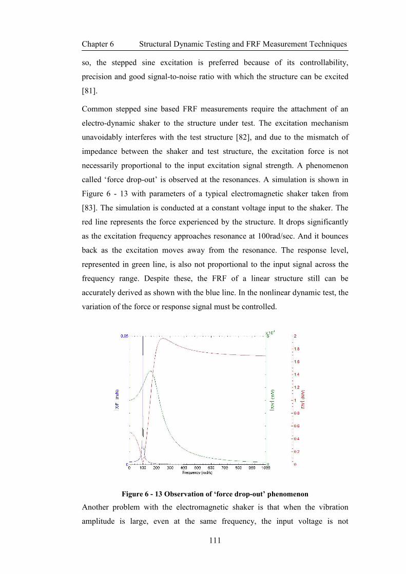
Chapter 6 Structural Dynamic Testing and FRF Measurement Techniques
111
so, the stepped sine excitation is preferred because of its controllability,
precision and good signal-to-noise ratio with which the structure can be excited
[81].
Common stepped sine based FRF measurements require the attachment of an
electro-dynamic shaker to the structure under test. The excitation mechanism
unavoidably interferes with the test structure [82], and due to the mismatch of
impedance between the shaker and test structure, the excitation force is not
necessarily proportional to the input excitation signal strength. A phenomenon
called ‘force drop-out’ is observed at the resonances. A simulation is shown in
Figure 6 - 13 with parameters of a typical electromagnetic shaker taken from
[83]. The simulation is conducted at a constant voltage input to the shaker. The
red line represents the force experienced by the structure. It drops significantly
as the excitation frequency approaches resonance at 100rad/sec. And it bounces
back as the excitation moves away from the resonance. The response level,
represented in green line, is also not proportional to the input signal across the
frequency range. Despite these, the FRF of a linear structure still can be
accurately derived as shown with the blue line. In the nonlinear dynamic test, the
variation of the force or response signal must be controlled.
Figure 6 - 13 Observation of ‘force drop-out’ phenomenon
Another problem with the electromagnetic shaker is that when the vibration
amplitude is large, even at the same frequency, the input voltage is not
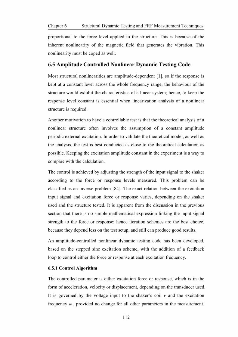
Chapter 6 Structural Dynamic Testing and FRF Measurement Techniques
112
proportional to the force level applied to the structure. This is because of the
inherent nonlinearity of the magnetic field that generates the vibration. This
nonlinearity must be coped as well.
6.5 Amplitude Controlled Nonlinear Dynamic Testing Code
Most structural nonlinearities are amplitude-dependent [1], so if the response is
kept at a constant level across the whole frequency range, the behaviour of the
structure would exhibit the characteristics of a linear system; hence, to keep the
response level constant is essential when linearization analysis of a nonlinear
structure is required.
Another motivation to have a controllable test is that the theoretical analysis of a
nonlinear structure often involves the assumption of a constant amplitude
periodic external excitation. In order to validate the theoretical model, as well as
the analysis, the test is best conducted as close to the theoretical calculation as
possible. Keeping the excitation amplitude constant in the experiment is a way to
compare with the calculation.
The control is achieved by adjusting the strength of the input signal to the shaker
according to the force or response levels measured. This problem can be
classified as an inverse problem [84]. The exact relation between the excitation
input signal and excitation force or response varies, depending on the shaker
used and the structure tested. It is apparent from the discussion in the previous
section that there is no simple mathematical expression linking the input signal
strength to the force or response; hence iteration schemes are the best choice,
because they depend less on the test setup, and still can produce good results.
An amplitude-controlled nonlinear dynamic testing code has been developed,
based on the stepped sine excitation scheme, with the addition of a feedback
loop to control either the force or response at each excitation frequency.
6.5.1 Control Algorithm
The controlled parameter is either excitation force or response, which is in the
form of acceleration, velocity or displacement, depending on the transducer used.
It is governed by the voltage input to the shaker’s coil v and the excitation
frequency ω , provided no change for all other parameters in the measurement.
Chapter 6 Structural Dynamic Testing and FRF Measurement Techniques
113
From the mathematical point of view, force and response can be controlled in a
similar fashion, so only the force control algorithm is presented here.
The desired force measured by the transducer, f, can be expressed in terms of ν
and ω described by an unknown function G:
( , )f v ω= G (6.2)
f and v can be expressed in Fourier Series:
1 1
n n in
n n
f f F e∞ ∞
Φ
= =
= =∑ ∑ (6.3)
1 1
n n in
n n
v v V e∞ ∞
Φ
= =
= =∑ ∑ (6.4)
In which nF and nV are the coefficients of the nth
harmonic terms after the force
and voltage signals are decomposed. Both nF and nV are complex terms. If a
number, m, of harmonics is considered, the force and voltage can be represented
by vectors of harmonic coefficients as:
1 1
2 2
m m
V F
V Fv f
V F
= =
⋮ ⋮ (6.5)
Equation (6.2) cannot be solved analytically because of the unknown nature of
the function G; however, it can be solved iteratively by converting to the
following equation:
( , )Gf v ω′= (6.6)
In which G′ is a transfer function linking two vectors. This equation can be
further expressed as:
( , ) ( , ) 0N Gv f vω ω′= − = (6.7)
Equation (6.7) is solved with Newton-Raphson method, which is chosen because
of its efficiency in convergence and ease of implementation. In practice, f is
predetermined as the desired excitation force amplitude, and the purpose of the

Chapter 6 Structural Dynamic Testing and FRF Measurement Techniques
114
iteration is to find the right value of v to satisfy equation (6.7). At a particular
excitation frequency, the resultant v after n iterations is:
( 1) ( ) ( ) 1 ( )[ ( )] ( )N Nn n n nv v v v+ −′= − (6.8)
in which ( )( )N nv′ is the Jacobian matrix, which is defined as:
1 1
1
( )
1
( )
N N
N
N N
m
n
m m
m
V V
v
V V
∂ ∂ ∂ ∂
′ = ∂ ∂ ∂ ∂
⋯
⋮ ⋱ ⋮
⋯
(6.9)
Here, all the partial derivatives are evaluated at ( )nv , namely,
( )( )N N
i i n
j j
v
V V
∂ ∂=
∂ ∂ (6.10)
It should be noticed that the Jacobian matrix here is non-singular so that its
inverse exists.
The function N is not known analytically, so its partial derivative can only be
approximated with a finite difference approach:
( )
( ) ( )( ) 1( ( ) ( ))
2
N NN N
i i ni n i n
j j j
vv h v h
V V H
∂ ∂= ≈ + − −
∂ ∂ (6.11)
in which jH is a small deviation from jV , and h is a column vector of length m,
with the thj element as jH and all the other elements zero.
Though mathematically a sound approach, experimentally it is difficult to get the
Jacobian matrix with equation (6.11) due to the following reasons:
• In order to get a very close approximation of the partial derivatives, the step
jH should be as small as possible; however, in experimental conditions, a
small change in jV may not induce a noticeable change in N, because of
unavoidable measurement limitations. In a worse case, the finite difference
approach with very small step size may give totally erroneous approximation
of the Jacobian matrix;

Chapter 6 Structural Dynamic Testing and FRF Measurement Techniques
115
• The unknown nature of the function N makes it difficult to define the best
step size jH ;
• 2m number of measurements are required at every frequency point in order to
determine the full Jacobian matrix. This is not practical if the number of
harmonics to be controlled is large.
In order to increase the speed of the control algorithm, mainly, to avoid the
direct calculation of partial derivatives, the Secant method [49] is used, which is
expressed as:
( ) ( 1)
( )
( ) ( 1)
( ) ( )( )
N NN
n nn
n n
v vv
v v
−
−
−′ ≈−
(6.12)
With the approximated Jacobian Matrix ( )( )N nv′ calculated, the voltage input to
the shaker ( 1)nv + is updated; so is the driving force to the nonlinear system.
As a starting point, and without losing the essence of Newton-Raphson based
algorithm described above, a main-harmonic amplitude controlled nonlinear
dynamic testing code has been developed in LabView. Figure 6 - 14 displays a
flowchart that the code is based on.
Figure 6 - 14 Schematic representation of nonlinear force control algorithm

Chapter 6 Structural Dynamic Testing and FRF Measurement Techniques
116
The user defines the following parameters beforehand: 0ω - starting excitation
frequency; ω∆ - frequency step; 0
1V - starting voltage of the driving signal; RF -
desired driving force; ε - error ratio. The nonlinear system in the above figure
physically includes the shaker, power amplifier, transducers and the testing
structure. Once the cyclic driving signal is released from the signal generator, the
force and response signals are recorded after a delay to allow settling, and both
signals go through an FFT or other Fourier decomposition to get the main
harmonic components. In this force-controlled case, the amplitude of the force
signal is compared with the desired force level. If the resultant error is within
tolerance, the FRF point is calculated and plotted. The driving signal will go to
the next excitation frequency.
If the error ratio limit is exceeded, the iteration process starts. The Secant
method requires inputs from the last two iterations, so for the first loop, a
proportional interpretation is used to derive the new driving signal amplitude.
The reason behind this is that normally the structure is tested starting from a
frequency away from any resonances, and at that frequency point, the nonlinear
structure displays properties close to linear ones; so the driving signal
corresponds with the force in a fairly linear fashion, and a proportional
interpretation is suitable. The signal generator is updated with a new amplitude
at the same frequency. The resultant force is compared with the desired value
again to decide whether a further iteration loop is needed or the FRF point
should be calculated. In the case that another iteration is needed, the Secant
method interpretation is used. The above described process is repeated until all
the FRF points within the frequency range have been obtained.
Besides the control algorithm, there are other points to be taken care of, which
are difficult to present in the above flow chart.
• The strength of the driving signal must be capped in order not to damage the
whole system accidentally;
• There are possibilities that the Newton-Raphson method fails to locate the
root, which is mathematically proven; hence, there must be a cap on the
number of loops the program is allowed to run at each frequency point;
Chapter 6 Structural Dynamic Testing and FRF Measurement Techniques
117
• The delay time should be set according to the properties of the tested structure.
For flexible and lightly damped structures, the delay time must be set long
enough to avoid any transient effect being counted;
• The transition from one frequency point to another, and from one amplitude
to another must be smooth. This is due to the fact that at around the resonance,
there are possibly more than one stable vibration states. If the transition is
abrupt, one steady state may not be captured completely in the frequency
range before the vibration jumps to another steady state. This will cause
incompletion in the FRF.
6.5.2 LabView Program for the Nonlinear Testing Code
Figure 6 - 15 Control panel of the nonlinear testing code in LabView
The above control algorithm was implemented in LabView, a software
development environment based on graphical programming from National
Instrument. Figure 6 - 15 shows the design control panel, on which the user can
adjust parameters to suit test requirement. One Hewlett Packard 33120A
Waveform Generator was used to generate driving signals and one National

Chapter 6 Structural Dynamic Testing and FRF Measurement Techniques
118
Instrument NI4472 Dynamic Signal Acquisition Card was used to acquire force
and response signals.
6.5.3 Further Improvement
Though the nonlinear testing code has been successfully implemented and
showed its reliability and accuracy in various applications, improvement is still
required. The main points are listed below:
• Instead of only the main-harmonic component being monitored and
controlled, super-harmonic and sub-harmonic components should also be
included in the code. The mathematical foundation has been laid down in
section 6.5.1;
• Newton-Raphson iteration can sometime fail to converge if the starting point
of the iteration is not well placed. Additional algorithm should be included in
the code so as to avoid this from happening;
• Structural dynamic testing, especially when nonlinearity is of concern,
requires a very good understanding of the theory and the test specimen itself
in order to achieve an efficient and error-free test. This requires the expertise
of a specialist. However, things can be made easier if the code can be made
smarter, e.g. the delay time can be automatically adjusted based on the
vibration data acquired.
6.6 Concluding Remarks
The basic knowledge involved in structural dynamic testing is examined in the
first half of this chapter. The fundamental message addressed is that it is
important and necessary to conduct dynamic tests, and to do so correctly. The
accuracy and correctness of the experiment measurements are dictated by the
capabilities of the transducers, data processing equipment and experimental
setup. Almost all methods for applying the structural excitation will have some
unwanted modification effects on the structure, as well, almost all the response
measurement transducers and support fixtures will have an unwanted influence
on the structure. Furthermore, many of the potential problems with dynamic tests
only become apparent during the actual tests. We should be aware of these
problems and strive to select methods to minimise these effects. In many

Chapter 6 Structural Dynamic Testing and FRF Measurement Techniques
119
respects the practice of vibration testing is more of an art than a science. There is
no single right way to perform a vibration test, as described by Maia etc. [16].
An amplitude controlled nonlinear dynamic testing code is introduced in the
second half. It is a natural extension to a linear one. Though relative simple in
concept, the implementation of the algorithm is rather troublesome. Some
achievements have been made, in terms of improving the reliability and safety
measures, reducing the test time and most importantly, fulfilling its purpose.
Nonetheless, more effort should be poured into this field, to develop it up to a
level of competency comparable to what linear dynamic test enjoys now.
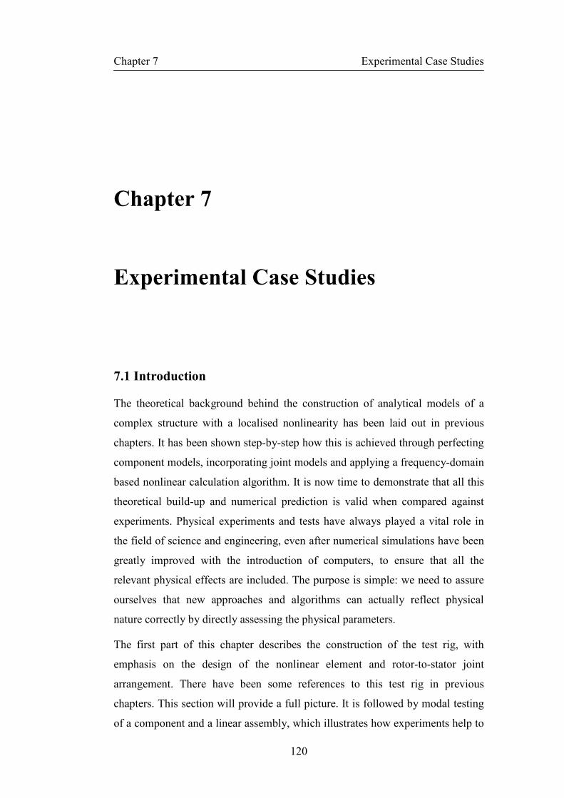
Chapter 7 Experimental Case Studies
120
Chapter 7
Experimental Case Studies
7.1 Introduction
The theoretical background behind the construction of analytical models of a
complex structure with a localised nonlinearity has been laid out in previous
chapters. It has been shown step-by-step how this is achieved through perfecting
component models, incorporating joint models and applying a frequency-domain
based nonlinear calculation algorithm. It is now time to demonstrate that all this
theoretical build-up and numerical prediction is valid when compared against
experiments. Physical experiments and tests have always played a vital role in
the field of science and engineering, even after numerical simulations have been
greatly improved with the introduction of computers, to ensure that all the
relevant physical effects are included. The purpose is simple: we need to assure
ourselves that new approaches and algorithms can actually reflect physical
nature correctly by directly assessing the physical parameters.
The first part of this chapter describes the construction of the test rig, with
emphasis on the design of the nonlinear element and rotor-to-stator joint
arrangement. There have been some references to this test rig in previous
chapters. This section will provide a full picture. It is followed by modal testing
of a component and a linear assembly, which illustrates how experiments help to

Chapter 7 Experimental Case Studies
121
improve the analytical models. Last but not least, amplitude controlled stepped-
sine sweep tests are presented to accurately measure the non-linearity, the results
of which are compared with numerical simulations.
It is worth mentioning here that constructing a test rig and conducting
experiments is not an easy and straightforward business. It might only be worth a
few pages of presentation in this thesis, but the time and effort involved is well
over its fair share.
7.2 Description of the Test Rig
Some considerations for the test rig at the design stage are:
• The test rig should have a reasonably complex nature in terms of geometry,
material properties, flexibility and functionality. It is aimed to be
representative of a real world structure. This is to differentiate from many
purpose-built and academic test rigs commonly seen in lab environments.
• The test rig should have a prominent and clearly-defined nonlinear element.
All the other nonlinear sources shall be minimised.
• The nonlinearity shall be adjustable. In the real world, nonlinearity can
change throughout the structure’s lifespan due to wear and tear, change of
operation conditions etc. The analytical models should be able to cope with
that and it is very appealing to have it in the test rig.
Figure 7 - 1 Overall test rig setup
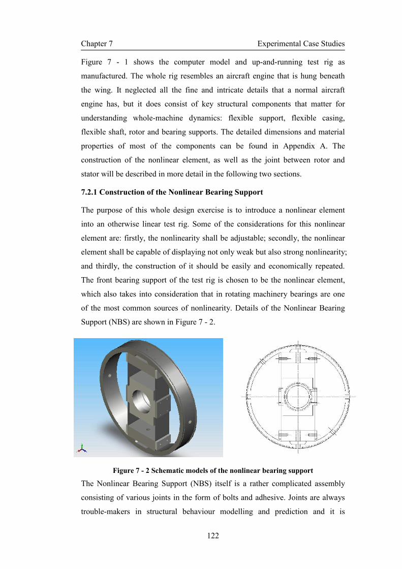
Chapter 7 Experimental Case Studies
122
Figure 7 - 1 shows the computer model and up-and-running test rig as
manufactured. The whole rig resembles an aircraft engine that is hung beneath
the wing. It neglected all the fine and intricate details that a normal aircraft
engine has, but it does consist of key structural components that matter for
understanding whole-machine dynamics: flexible support, flexible casing,
flexible shaft, rotor and bearing supports. The detailed dimensions and material
properties of most of the components can be found in Appendix A. The
construction of the nonlinear element, as well as the joint between rotor and
stator will be described in more detail in the following two sections.
7.2.1 Construction of the Nonlinear Bearing Support
The purpose of this whole design exercise is to introduce a nonlinear element
into an otherwise linear test rig. Some of the considerations for this nonlinear
element are: firstly, the nonlinearity shall be adjustable; secondly, the nonlinear
element shall be capable of displaying not only weak but also strong nonlinearity;
and thirdly, the construction of it should be easily and economically repeated.
The front bearing support of the test rig is chosen to be the nonlinear element,
which also takes into consideration that in rotating machinery bearings are one
of the most common sources of nonlinearity. Details of the Nonlinear Bearing
Support (NBS) are shown in Figure 7 - 2.
Figure 7 - 2 Schematic models of the nonlinear bearing support
The Nonlinear Bearing Support (NBS) itself is a rather complicated assembly
consisting of various joints in the form of bolts and adhesive. Joints are always
trouble-makers in structural behaviour modelling and prediction and it is

Chapter 7 Experimental Case Studies
123
preferable to reduce the number of joints in the test rig to minimise calculation
complexity; nevertheless, they are unavoidable in most practical cases. It is
assumed, and later on shown in the experimental results, that the effect of local
joints in the NBS on the whole assembly can be neglected.
The whole NBS is first manufactured in pieces as shown in Figure 7 - 3(a). The
two 0.5mm spring-steel plates, running parallel (shown vertically in Figure 7 -
3(b)) are then glued to the two fixing blocks as well as the bearing block using
Araldite2011, a multi-purpose epoxy which bonds Ferrous metal and
Aluminium excellently. The bearing block is located at the exact mid-span of the
spring-steel plates. Some 5mm-thick steel plates are used to sandwich the spring-
steel plates to prevent them peeling off. Drilled holes are threaded though the
fixing plates and into the fixing blocks as well as the bearing block, to give the
spring-steel plates a final security. This part of the NBS is then fastened to the
outer rim, with which, a completed NBS is constructed. The final assembly is
shown in Figure 7 - 3(c). At a later stage, a bearing will be fitted into the bearing
block.
When not stressed, the combination of the spring-steel plates and the bearing
block acts as an asymmetric joint to the rotor supported, with different linear
stiffness in the vertical and horizontal directions: stiffer in the ‘vertical’ and
softer in the ‘horizontal’ direction. Cubic stiffness nonlinearity will be present in
the horizontal direction when the displacement is large. The spring-steel plates
can be bent slightly by reducing the distance between the two fixing ends. This is
achieved by inserting shim plates between the rim and the fixing blocks. A shim
plate is basically a thin piece of stainless steel that is normally used to fill small
gaps or spaces between objects. In this application, it is used to accurately reduce
the distance between the two fixing blocks. As a result of this arrangement, the
bearing support displays a stiffness pattern governed by the buckling effect of
the spring-steel plates.
The beauty of this assembly, despite the complexity caused by the connections,
is the ease of changing the configuration to display different dynamic properties.
For example, the spring-steel plates can easily be replaced with other types of
plates to produce different patterns of stiffness distribution. Furthermore, the
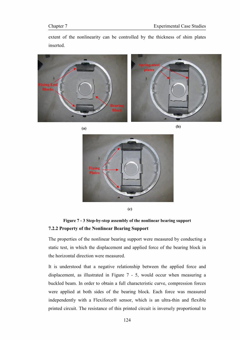
Chapter 7 Experimental Case Studies
124
extent of the nonlinearity can be controlled by the thickness of shim plates
inserted.
Figure 7 - 3 Step-by-step assembly of the nonlinear bearing support
7.2.2 Property of the Nonlinear Bearing Support
The properties of the nonlinear bearing support were measured by conducting a
static test, in which the displacement and applied force of the bearing block in
the horizontal direction were measured.
It is understood that a negative relationship between the applied force and
displacement, as illustrated in Figure 7 - 5, would occur when measuring a
buckled beam. In order to obtain a full characteristic curve, compression forces
were applied at both sides of the bearing block. Each force was measured
independently with a Flexiforce® sensor, which is an ultra-thin and flexible
printed circuit. The resistance of this printed circuit is inversely proportional to
Fixing End
Blocks
Bearing
Block
Spring-steel
plates
Fixing
Plates
(a) (b)
(c)

Chapter 7 Experimental Case Studies
125
the normal force applied. The difference between the two forces applied at both
sides of the bearing block is the static force experienced by the nonlinear bearing
block at the centre.
When shim plates are not used, the stiffness measured is of typical 3rd
order
nonlinearity that is encountered when material deformation is large and exceeds
the linear assumption of stress and strain relationship. Figure 7 - 4 shows the
measurement result, in which the y-axis is the force and the x-axis is the
displacement. The red circles are the measurement points, and the blue line is the
best fitting curve. The best fitting curve can be expressed with a 3rd order
polynomial equation 3
1 3nF k x k x= + , in which 4
1 2.544 10 N/mk = × and
9 3
3 2.574 10 N/mk = × .
Figure 7 - 4 Nonlinear characteristic of the nonlinear bearing support without
shim plate
When shim plates of combined thickness of 0.4mm were used, the spring steel
plates were in a buckled state. The measurement results are shown in Figure 7 -
5, The best fitting curve can be mathematically expressed as: 3
1 3nF k x k x= + . The
stiffness parameters 4
1 1.265 10 N/mk = − × and 9 3
3 1.381 10 N/mk = × were
obtained by minimising the discrepancy between measured and approximated
values. Point A is the global geometric centre and in this case is an unstable
equilibrium point; B and C are two stable equilibrium points.

Chapter 7 Experimental Case Studies
126
Figure 7 - 5 Nonlinear characteristic of the nonlinear bearing support with 0.4mm
shim plates
7.2.3 Construction of the Rotor-Stator Connections
The design of the connection between the rotor and the stator is not insignificant
and warrants a special mention here. As the primary purpose of this test rig is to
demonstrate the analytical modelling capability for a complicated structure with
localised nonlinearity, it is useful to have a single and prominent nonlinearity
and to minimise any ‘side’ effects that will complicate the calculation as well as
the demonstration. In rotating equipment, the joints between the rotor and stator
are often the sources of nonlinearity and uncertainty. This is mainly due to the
fact that tight tolerance is difficult to achieve. In normal operation the clearance
between the rotor and stator does not cause any problems. However, when
performing vibration tests, even a very small amount of clearance can cause
rattling and distort the results [61]. One place of major concern is the connection
between the shaft and bearing.
A collet and its associated two-piece adaptor shown in Figure 7 - 6 is used to
secure the shaft to the bearing. The collet is normally found in a machine tool’s
rotating spindle as part of a holding device. It has a gentle tapered outer surface
and a uniform inner surface which forms a collar around the object to be held.
As the two-piece adaptor is tightened, a strong clamping force is exerted onto the
object that prevents any gap and sliding movement. Because tightening and
securing the collet onto shaft is a gentle and uniform process, it gives good
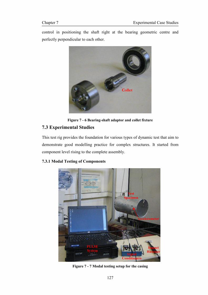
Chapter 7 Experimental Case Studies
127
control in positioning the shaft right at the bearing geometric centre and
perfectly perpendicular to each other.
Figure 7 - 6 Bearing-shaft adaptor and collet fixture
7.3 Experimental Studies
This test rig provides the foundation for various types of dynamic test that aim to
demonstrate good modelling practice for complex structures. It started from
component level rising to the complete assembly.
7.3.1 Modal Testing of Components
Figure 7 - 7 Modal testing setup for the casing
Impact
Hammer
Test
Specimen
PULSE
System
Accelerometer
Signal
Conditioners
Collet

Chapter 7 Experimental Case Studies
128
All the major components of the test rig: casing, rotor, shaft and bearing supports,
have been modal tested and validated. This is a very necessary step to achieve a
accurate assembly model in the end. Only the modal test on the casing is
presented here, while the technique, equipment, data acquisition and processing
routine are the same across all the tests.
Figure 7 - 7 shows the setup for impact tests on the casing. The dimensional and
material properties of the casing can be found in Appendix A. The casing is
suspended at the end of a bungee cord, which adds minimum rigidity to the
casing. It is reasonable to assume that the casing is supported at free-free
boundary condition. The PCB ICP® Impulse Force Test Hammer 086C02 is
used to provide the impulse excitation, which consists of a nearly constant force
over a broad frequency range and is capable of exciting all resonances in that
range. The size of the hammer, hardness of the tip and velocity at impact
determine the amplitude and frequency content of the force impulse. It is from
the preliminary FE calculation and good understanding of the experiment itself
that the best combination is chosen. The accelerometer used is PCB ICP®
Accelerometer 352C67. Both force and acceleration signals are fed through
battery-powered PCB ICP® sensor signal conditioners, which amplify the
signals to be readable by the analyser. The PULSE™ system from Brüel & Kjær
is used for data acquisition and processing. The system consists of a piece of
front-end data acquisition system with anti-aliasing filters, which conditions and
digitises the transducer signals, and a computer with PULSE operation software
that allows real time acquisition, recording and processing of data. Different
types of analysers are available. For the impact tests, the FFT analyser is used.
Calibration of the transducers followed the similar procedures as in Section 6.3.2.
The modal testing process starts by specifying measurement points on the
structure. The number and location of those points chosen affects the resolution
of mode shape comparison later on, which is a key factor to determine whether
an FE model is valid. In this experiment, 81 grid points on the outer surface of
the casing are selected, the location of which is measured and a 3D frame model
is constructed using ICATS [85], as shown in Figure 7 - 8. ICATS is a Modal
Analysis software package developed in Imperial College London. It extracts
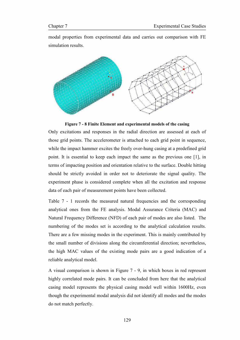
Chapter 7 Experimental Case Studies
129
modal properties from experimental data and carries out comparison with FE
simulation results.
Figure 7 - 8 Finite Element and experimental models of the casing
Only excitations and responses in the radial direction are assessed at each of
those grid points. The accelerometer is attached to each grid point in sequence,
while the impact hammer excites the freely over-hung casing at a predefined grid
point. It is essential to keep each impact the same as the previous one [1], in
terms of impacting position and orientation relative to the surface. Double hitting
should be strictly avoided in order not to deteriorate the signal quality. The
experiment phase is considered complete when all the excitation and response
data of each pair of measurement points have been collected.
Table 7 - 1 records the measured natural frequencies and the corresponding
analytical ones from the FE analysis. Modal Assurance Criteria (MAC) and
Natural Frequency Difference (NFD) of each pair of modes are also listed. The
numbering of the modes set is according to the analytical calculation results.
There are a few missing modes in the experiment. This is mainly contributed by
the small number of divisions along the circumferential direction; nevertheless,
the high MAC values of the existing mode pairs are a good indication of a
reliable analytical model.
A visual comparison is shown in Figure 7 - 9, in which boxes in red represent
highly correlated mode pairs. It can be concluded from here that the analytical
casing model represents the physical casing model well within 1600Hz, even
though the experimental modal analysis did not identify all modes and the modes
do not match perfectly.
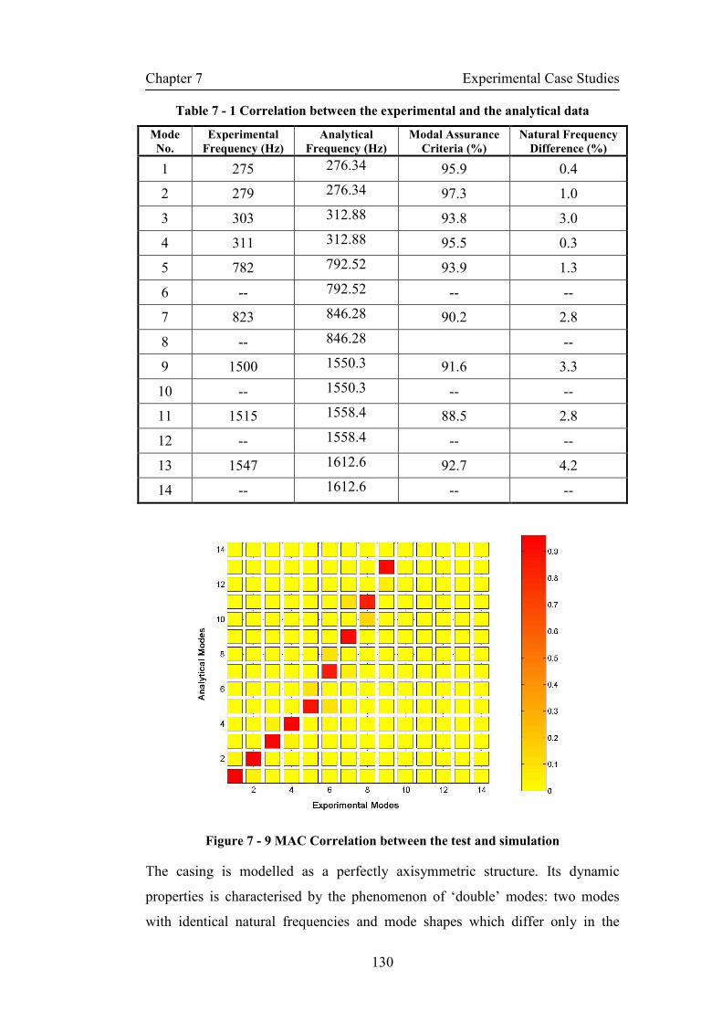
Chapter 7 Experimental Case Studies
130
Table 7 - 1 Correlation between the experimental and the analytical data
Mode
No.
Experimental
Frequency (Hz)
Analytical
Frequency (Hz)
Modal Assurance
Criteria (%)
Natural Frequency
Difference (%)
1 275 276.34 95.9 0.4
2 279 276.34 97.3 1.0
3 303 312.88 93.8 3.0
4 311 312.88 95.5 0.3
5 782 792.52 93.9 1.3
6 -- 792.52 -- --
7 823 846.28 90.2 2.8
8 -- 846.28 --
9 1500 1550.3 91.6 3.3
10 -- 1550.3 -- --
11 1515 1558.4 88.5 2.8
12 -- 1558.4 -- --
13 1547 1612.6 92.7 4.2
14 -- 1612.6 -- --
Figure 7 - 9 MAC Correlation between the test and simulation
The casing is modelled as a perfectly axisymmetric structure. Its dynamic
properties is characterised by the phenomenon of ‘double’ modes: two modes
with identical natural frequencies and mode shapes which differ only in the
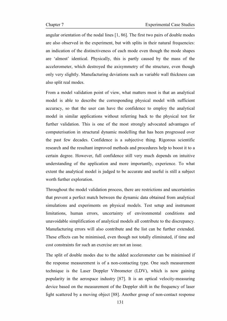
Chapter 7 Experimental Case Studies
131
angular orientation of the nodal lines [1, 86]. The first two pairs of double modes
are also observed in the experiment, but with splits in their natural frequencies:
an indication of the distinctiveness of each mode even though the mode shapes
are ‘almost’ identical. Physically, this is partly caused by the mass of the
accelerometer, which destroyed the axisymmetry of the structure, even though
only very slightly. Manufacturing deviations such as variable wall thickness can
also split real modes.
From a model validation point of view, what matters most is that an analytical
model is able to describe the corresponding physical model with sufficient
accuracy, so that the user can have the confidence to employ the analytical
model in similar applications without referring back to the physical test for
further validation. This is one of the most strongly advocated advantages of
computerisation in structural dynamic modelling that has been progressed over
the past few decades. Confidence is a subjective thing. Rigorous scientific
research and the resultant improved methods and procedures help to boost it to a
certain degree. However, full confidence still very much depends on intuitive
understanding of the application and more importantly, experience. To what
extent the analytical model is judged to be accurate and useful is still a subject
worth further exploration.
Throughout the model validation process, there are restrictions and uncertainties
that prevent a perfect match between the dynamic data obtained from analytical
simulations and experiments on physical models. Test setup and instrument
limitations, human errors, uncertainty of environmental conditions and
unavoidable simplification of analytical models all contribute to the discrepancy.
Manufacturing errors will also contribute and the list can be further extended.
These effects can be minimised, even though not totally eliminated, if time and
cost constraints for such an exercise are not an issue.
The split of double modes due to the added accelerometer can be minimised if
the response measurement is of a non-contacting type. One such measurement
technique is the Laser Doppler Vibrometer (LDV), which is now gaining
popularity in the aerospace industry [87]. It is an optical velocity-measuring
device based on the measurement of the Doppler shift in the frequency of laser
light scattered by a moving object [88]. Another group of non-contact response
Chapter 7 Experimental Case Studies
132
measurement devices are based on principles in electric circuits, e.g. change of
inductance, eddy current and capacity etc. due to the change of the gap between
the sensor and the object [89]. The unfavourable side of the LDV is the cost of
dedicated equipment required is still very high; as well the measurement can
only be made in the line of sight. The latter methods require the transducer to be
fixed to a frame, which may be moving, hence the transducer measures the
relative displacement, whereas an accelerometer measures the absolute
acceleration. In addition, the test preparation is much more time-consuming and
the operation environment requirement is much more stringent comparing to the
tests using traditional piezoelectric-based accelerometers. From the analytical
model side, the model can be made as complicated as possible to include all
expected test parameters, e.g. considering additional mass and stiffness due to
the accelerometer and more realistic boundary conditions.
The analytical model can be further improved by applying model updating
methods. The Inverse Eigensensitivity method described in Chapter Two was
employed here. Either eigenvectors or eigenvalues can be used; the former tends
to be more complicated and used more often in updating local parameters. For a
geometrically simple component with homogenous material properties like the
casing, global parameters, e.g. physical size, material density and Young’s
Modulus, are more often of updating value. Another consideration is which one
of the two, eigenvalue or eigenvector, is more likely affected by experimental
inaccuracy. There is no point to update parameters to a certain level of accuracy
while the reference parameter, eigenvalue or eigenvector in this case, cannot be
measured with a higher accuracy. The derivation of eigenvectors, or mode shape
information, from experiments could suffer imperfection due to slight inaccuracy
in marking grid points on the casing surface and non-perfect hammer impact on
a curved surface. On the other hand, eigenvalues, or natural frequencies, could
usually be measured more accurately; hence they were chosen as the reference
parameter.
The natural frequencies after five iterations, with the Young’s modulus as the
updating parameter, is shown in Table 7 - 2. The iteration aimed to minimise the
average Natural Frequency Difference (NFD) . It is reduced from 2.24% to
1.31%.
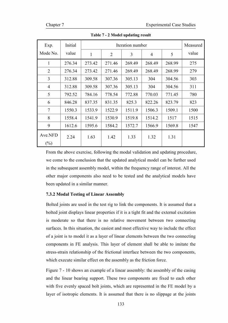
Chapter 7 Experimental Case Studies
133
Table 7 - 2 Model updating result
Iteration number Exp.
Mode No.
Initial
value 1 2 3 4 5
Measured
value
1 276.34 273.42 271.46 269.49 268.49 268.99 275
2 276.34 273.42 271.46 269.49 268.49 268.99 279
3 312.88 309.58 307.36 305.13 304 304.56 303
4 312.88 309.58 307.36 305.13 304 304.56 311
5 792.52 784.16 778.54 772.88 770.03 771.45 780
6 846.28 837.35 831.35 825.3 822.26 823.79 823
7 1550.3 1533.9 1522.9 1511.9 1506.3 1509.1 1500
8 1558.4 1541.9 1530.9 1519.8 1514.2 1517 1515
9 1612.6 1595.6 1584.2 1572.7 1566.9 1569.8 1547
Ave.NFD
(%)
2.24 1.63 1.42 1.33 1.32 1.31
From the above exercise, following the modal validation and updating procedure,
we come to the conclusion that the updated analytical model can be further used
in the subsequent assembly model, within the frequency range of interest. All the
other major components also need to be tested and the analytical models have
been updated in a similar manner.
7.3.2 Modal Testing of Linear Assembly
Bolted joints are used in the test rig to link the components. It is assumed that a
bolted joint displays linear properties if it is a tight fit and the external excitation
is moderate so that there is no relative movement between two connecting
surfaces. In this situation, the easiest and most effective way to include the effect
of a joint is to model it as a layer of linear elements between the two connecting
components in FE analysis. This layer of element shall be able to imitate the
stress-strain relationship of the frictional interface between the two components,
which execute similar effect on the assembly as the friction force.
Figure 7 - 10 shows an example of a linear assembly: the assembly of the casing
and the linear bearing support. These two components are fixed to each other
with five evenly spaced bolt joints, which are represented in the FE model by a
layer of isotropic elements. It is assumed that there is no slippage at the joints

Chapter 7 Experimental Case Studies
134
and the force applied does not exceed the material’s limit so that the linear
constitutive equations for these elements still hold. Fundamentally, the joints are
treated in the same manner as other structural components, with the only
difference being that the thin layer element’s material properties need to be
identified via experiment, the value is initially set to be the same as the
components’.
Figure 7 - 10 Finite Element and experimental models of a linear assembly
The experimental setup and analysis procedure are the same as the ones
employed for the component tests in the previous section. 118 grid points are
chosen as the measurement points as shown in Figure 7 - 10. The test results and
comparison are presented in Table 7 - 3. In each case the experimental modal
analysis has only located one of the pairs of symmetrical modes.
Table 7 - 3 Correlation between the experimental and the initial analytical data
Mode
No.
Experimental
Frequency (Hz)
Analytical
Frequency (Hz)
Modal Assurance
Criteria (%)
Natural Frequency
Difference (%)
1 287.7 301.3 95.1 4.73
2 -- 301.3 -- --
3 798.2 838.4 89.9 5.04
4 -- 838,4 -- --
5 1259.5 1360.6 93.7 8.03
6 -- 1360.6 -- --
7 -- 1646.1 -- --
8 1515.6 1646.1 87.5 8.61
Thin Layer
FE Model Exp. Model
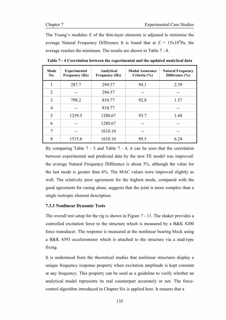
Chapter 7 Experimental Case Studies
135
The Young’s modulus E of the thin-layer elements is adjusted to minimise the
average Natural Frequency Difference It is found that at E = 15x109Pa, the
average reaches the minimum. The results are shown in Table 7 - 4.
Table 7 - 4 Correlation between the experimental and the updated analytical data
Mode
No.
Experimental
Frequency (Hz)
Analytical
Frequency (Hz)
Modal Assurance
Criteria (%)
Natural Frequency
Difference (%)
1 287.7 294.57 94.1 2.39
2 -- 294.57 -- --
3 798.2 810.77 92.8 1.57
4 -- 810.77 --
5 1259.5 1280.67 93.7 1.68
6 -- 1280.67 -- --
7 -- 1610.10 -- --
8 1515.6 1610.10 89.5 6.24
By comparing Table 7 - 3 and Table 7 - 4, it can be seen that the correlation
between experimental and predicted data by the new FE model was improved:
the average Natural Frequency Difference is about 3%, although the value for
the last mode is greater than 6%. The MAC values were improved slightly as
well. The relatively poor agreement for the highest mode, compared with the
good agreement for casing alone, suggests that the joint is more complex than a
single isotropic element description.
7.3.3 Nonlinear Dynamic Tests
The overall test setup for the rig is shown in Figure 7 - 11. The shaker provides a
controlled excitation force to the structure which is measured by a B&K 8200
force transducer. The response is measured at the nonlinear bearing block using
a B&K 4393 accelerometer which is attached to the structure via a stud-type
fixing.
It is understood from the theoretical studies that nonlinear structures display a
unique frequency response property when excitation amplitude is kept constant
at any frequency. This property can be used as a guideline to verify whether an
analytical model represents its real counterpart accurately or not. The force-
control algorithm introduced in Chapter Six is applied here. It ensures that a

Chapter 7 Experimental Case Studies
136
Figure 7 - 11 Overall setup of the test rig and the measurement system
constant excitation force is applied to the structure at every excitation frequency
point. The waveform is generated via the HP 33120A function generator which
has the capability of changing the clock rate of the output signal without
discontinuity. This property is essential because if there is a burst between
waveforms when the frequency progresses, a long settling time is required for
Power Amplifier
Charge Amplifiers
Signal Generator and Controller
Unit
Force Transducer
Accelerometer
Shaker
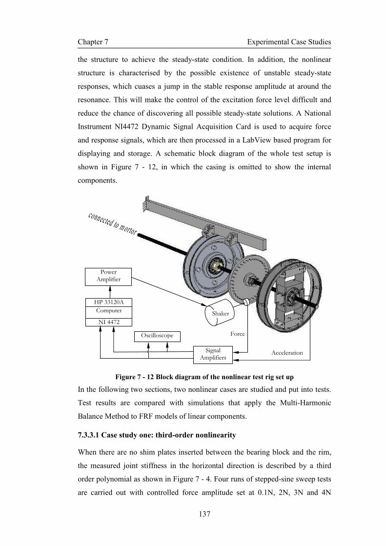
Chapter 7 Experimental Case Studies
137
the structure to achieve the steady-state condition. In addition, the nonlinear
structure is characterised by the possible existence of unstable steady-state
responses, which cuases a jump in the stable response amplitude at around the
resonance. This will make the control of the excitation force level difficult and
reduce the chance of discovering all possible steady-state solutions. A National
Instrument NI4472 Dynamic Signal Acquisition Card is used to acquire force
and response signals, which are then processed in a LabView based program for
displaying and storage. A schematic block diagram of the whole test setup is
shown in Figure 7 - 12, in which the casing is omitted to show the internal
components.
Figure 7 - 12 Block diagram of the nonlinear test rig set up
In the following two sections, two nonlinear cases are studied and put into tests.
Test results are compared with simulations that apply the Multi-Harmonic
Balance Method to FRF models of linear components.
7.3.3.1 Case study one: third-order nonlinearity
When there are no shim plates inserted between the bearing block and the rim,
the measured joint stiffness in the horizontal direction is described by a third
order polynomial as shown in Figure 7 - 4. Four runs of stepped-sine sweep tests
are carried out with controlled force amplitude set at 0.1N, 2N, 3N and 4N
Power Amplifier
Computer
HP 33120A
NI 4472
Signal Amplifiers
Shaker
Oscilloscope Force
Acceleration

Chapter 7 Experimental Case Studies
138
respectively. The results are presented in Figure 7 - 13. The sweeps started from
5Hz to 80Hz with step size of 0.2Hz. In each run, four modes are clearly
identified within the test frequency range. The influence of the nonlinearity is
manifested in the slightly distorted FRF curves at mode 2 and 3. The peaks bend
over to the higher frequency side as the excitation force level increases, an
indication of hardening stiffness as expected. Mode 1 and 4 do not seem to be
affected by the joint nonlinearity.
Figure 7 - 13 Measured FRFs for the 3rd
order nonlinearity case
Modal analysis carried out on the FE model of the test rig with equivalent linear
stiffness at the Nonlinear Bearing Support reveals why mode 1 and 4 are not
affected by the nonlinearity. Figure 7 - 14 shows the mode shapes of the four
modes. In each plot, the black wireframe model is the rig at rest condition and
the blue wireframe model is the maximum deformation at the corresponding
natural frequency. The scale of the deformations has been adjusted for clearer
presentation.
Modes 1 and 4 are the first and second horizontal bending modes of the whole
rig. The relative movement of the nonlinear bearing support is minimum and
negligible. Mode 2 is the first bending mode of the spring steel plates supporting
the bearing block, at which the nonlinear effect should be most prominent. Mode
3 is the swaying mode of the test rig and it includes deformation of the spring

Chapter 7 Experimental Case Studies
139
steel plates supporting the bearing block, suggesting that the nonlinearity will
also affect this mode.
(a) (b)
(c) (d)
Figure 7 - 14 First four modes of the linearised FE model of the test rig
Finer sweep tests were carried out to identify clearly the shift of the resonant
frequency of mode 2. Figure 7 - 15 shows the results of four sweeps with
different excitation forces. The solid lines are derived from the simulation using
the Multi-Harmonic Balance Method for comparison. The simulation results
agree with the test very well.
7.3.3.2 Case study two: second-order nonlinearity
After 0.4mm shim plates have been inserted between the bearing block and the
rim of the nonlinear bearing support, the bearing block rests at one of its two off-
centre stable points, B or C as indicated in Figure 7 - 5. When the excitation is
Mode 1 Mode 2
Mode 3 Mode 4

Chapter 7 Experimental Case Studies
140
small, the vibration of the bearing block is restricted to the local proximity of the
stable point. Around the stable point, for example point B along the stiffness
characteristic curve, the stiffness has a 2nd
order nonlinearity. This property is
evident from the plot below, in which a 2nd
order polynomial curve in red-dot fits
well to the measured characteristic curve in blue line around the stable point B;
hence it would be expected that a weakened stiffness characteristics would be
shown in the FRF curves.
Figure 7 - 15 Comparison of FRFs for the 3rd
order nonlinearity case
Figure 7 - 16 Indication of the 2
nd order nonlinearity
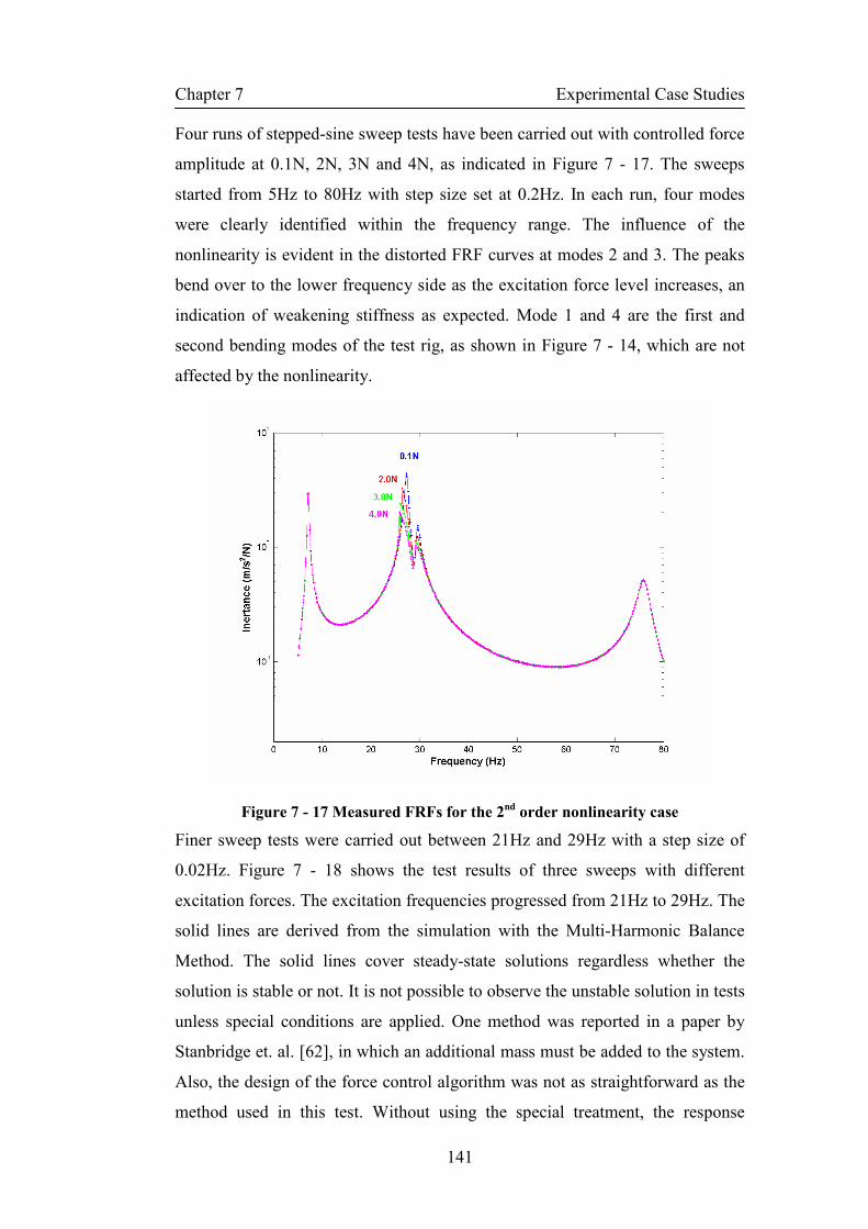
Chapter 7 Experimental Case Studies
141
Four runs of stepped-sine sweep tests have been carried out with controlled force
amplitude at 0.1N, 2N, 3N and 4N, as indicated in Figure 7 - 17. The sweeps
started from 5Hz to 80Hz with step size set at 0.2Hz. In each run, four modes
were clearly identified within the frequency range. The influence of the
nonlinearity is evident in the distorted FRF curves at modes 2 and 3. The peaks
bend over to the lower frequency side as the excitation force level increases, an
indication of weakening stiffness as expected. Mode 1 and 4 are the first and
second bending modes of the test rig, as shown in Figure 7 - 14, which are not
affected by the nonlinearity.
Figure 7 - 17 Measured FRFs for the 2nd
order nonlinearity case
Finer sweep tests were carried out between 21Hz and 29Hz with a step size of
0.02Hz. Figure 7 - 18 shows the test results of three sweeps with different
excitation forces. The excitation frequencies progressed from 21Hz to 29Hz. The
solid lines are derived from the simulation with the Multi-Harmonic Balance
Method. The solid lines cover steady-state solutions regardless whether the
solution is stable or not. It is not possible to observe the unstable solution in tests
unless special conditions are applied. One method was reported in a paper by
Stanbridge et. al. [62], in which an additional mass must be added to the system.
Also, the design of the force control algorithm was not as straightforward as the
method used in this test. Without using the special treatment, the response

Chapter 7 Experimental Case Studies
142
amplitude will jump at a frequency at which the steady-state solution becomes
unstable. In the stepped-sine sweep test with 4.0N constant excitation force, the
response amplitude jumped at 25.7Hz. The response amplitude jump is also
observed in Figure 7 - 19, in which the stepped-sine sweeps start from 29Hz, i.e.
sweep down in frequency.
Figure 7 - 18 Comparison of FRFs for the 2nd
order nonlinearity case – sweep up
Figure 7 - 19 Comparison of FRFs for the 3rd
order nonlinearity case - sweep down
Chapter 7 Experimental Case Studies
143
The combination of Figure 7 - 18 and Figure 7 - 19, i.e. the sweep-up and sweep-
down tests provides a full picture of steady-state response of such a nonlinear
system in a practical situation.
7.3.3.3 Discussion of the nonlinear tests
The original idea behind the design of the Nonlinear Bearing Support was that it
could display an adjustable nonlinearity and could be excited over its full
operation range. A strong nonlinearity was achieved by compressing the steel
strips into a slight buckled state, at which there existed non-stable negative
stiffness. Analytically the steady-state solution of a system with such
nonlinearity can be worked out using the Multi-Harmonic Balance Method, as
demonstrated in Chapter Five; however as experienced by the author the steady-
state response of such a system was difficult to achieve in experiment. The
reasons, concluded after several failed attempts, are: firstly, large excitation
force and shaker stroke are necessary in order to move the nonlinear bearing
support over its full operation range. This requires either a large shaker or an
additional control algorithm to compensate the force-displacement distortion
inherited in the shaker due to the requirement for large stroke. This is especially
true near the resonance frequencies. Secondly, there are multiple steady-state
solutions at frequencies near the resonance. Initial conditions decide which
steady-state solution the system will end up after the transient response decays
away. The ‘transient’ stage in this case refers to the stage when the response tries
to settle down on one steady-state solution while moving continuously from one
steady-state solution to another. This transient response, or rather the
‘undetermined’ stage of the response requires much longer and basically
unpredictable time to settle down, if ever it does. The requirement for the control
algorithm to cope with such a property is very high.
In the two experimental case studies, the control algorithm showed stable
operation and fast convergence when only the main harmonic component in the
excitation was controlled. It would be ideal and also technically possible to
control and keep the higher harmonics at zero; nevertheless the iteration and
calculation would slow down the measurement, and as observed during the
experiment, the higher harmonic components contributed only a few percent of
Chapter 7 Experimental Case Studies
144
the total amplitude of the vibration at resonance. Therefore, it is reasonable to
keep only the main harmonic terms in the experiment.
The damping of the nonlinear bearing support has not been mentioned in this
thesis, for the purpose of simplifying the whole problem and focusing only on
the nonlinearity in the stiffness. However, it does affect the prediction of the
steady-state solutions. In this thesis work, a structural damping ratio of 0.05 was
assigned to the joint, and indeed the prediction matches very nicely with the
experiment result.
7.4 Concluding Remarks
The main theme of this thesis is about complex structural assembly modelling. It
is not only about choosing the best available practices in mathematical modelling
but also about carrying out systematic experiments to verify the analytical
models. A fairly complicated test rig was designed and manufactured for such a
purpose. It consists of key elements typical to complex structural assemblies:
flexible components, semi-rigid connections and nonlinear elements. Dynamic
tests were carried out on components, linear assemblies and nonlinear assemblies
to measure steady-state responses which had good agreement with analytical
analysis results.

Chapter 8 Conclusions and Future Work
145
Chapter 8
Conclusions and Future Work
8.1 Conclusion of the Research Work
The problem studied in this research originated from real life applications: we
need a comprehensive methodology to model accurately and efficiently the
dynamics of a complex structural assembly, such as a rotating machine, and the
predictions from the assembly should be validated against experiments whenever
possible. A bottom-up process was used in this thesis. It is similar to a product
assembly line. It starts from small parts that have been manufactured to agreed
standards. With properly-designed connection mechanisms, it eventually grows
in complexity and completeness. The key for a high-quality final product relies
on the high quality components and integration scheme. Similarly, in the
structural modelling process, we need to take good care of components, linear
joints, nonlinear joints and coupling algorithms in order to get a satisfactory final
assembly model.
Each of the above topics can be studied relatively separately, and to a depth
beyond the reach of a single thesis work. Rather, this thesis takes a step back and
looks into how each can be best combined to serve the overall purpose of
producing a ‘reliable’ model.

Chapter 8 Conclusions and Future Work
146
It is believed that in practical situations, ‘real’ loadings are not really known,
material characteristics cannot be exactly predicted, and knowledge of how a
structure actually works is imprecise because of the complexity; hence analytical
models carrying uncertainty information are best for predicting and explaining
the structural behaviour. Uncertainty definitely exists, but the boundary between
certainty and uncertainty is not fixed. New techniques, methods and procedures
can help to improve our grasp of the definite truth and push the boundary further
into previously uncertain territory. It is the author’s firm belief that we need to
concentrate on perfecting our understanding of the definite world before resort to
those uncertainty theories.
8.1.1 Conclusion on the Modelling of Linear Structures
Theories and methods behind linear structural modelling have already been well
developed. It might seem to be quite basic nowadays, but it is crucial to get the
fundamentals right before we embark on more complicated problems.
The Finite Element Method has been the dominant method to construct the
fundamental Spatial model, from which the Modal model and Response model
can be derived analytically if the structure can be considered to be linear. Theses
three types of model representations are the key in structural dynamics analysis,
because they are interrelated and can be derived from experiments on real
structures. This provides the basis for validating the analytical model.
Model validation is a necessary step towards achieving an accurate component
model. It is a way to minimise the uncertainty at the component level. The
casing example discussed in Section 7.3.1 showed that the original value of one
of the material properties, Young’s Modulus, was not very accurate, possibly
due to the uncertainty of the exact alloy used or processing at the manufacturing
stage. This value was improved by carrying out a model updating process, after
which the dynamic properties from both prediction and test were brought closer
to each other. No perfect match was achieved though; this was attributed to the
test method used, possible dimension variability in the thickness etc.
8.1.2 Conclusion on Joint Representations
Mechanical joints have all along been a difficult subject to study because of the
large amount of variety and the complex physics they involve. If all the fine
Chapter 8 Conclusions and Future Work
147
details of a joint are included in the model, the resultant assembly model will be
very large and efficient analysis of it will be a problem. Therefore some
simplifications must be carried out. The aim is to provide manageable but
realistic joint models to the whole assembly model at minimum cost.
Linearisation is the first type of simplification. Mechanical joints, even though
their behaviour are better described as nonlinear, can sometimes still be
considered as linear at normal operation conditions. They can be represented in
the same way as other linear structural components, in the form of symmetric
system matrices. The direct construction of such matrices can be tedious; hence
using an FE model to model a joint is a convenient alternative. The advantage of
the FE joint model is that it can be readily integrated with the remaining
structural FE models. An example has been shown in Section 7.3.2 with such
application. After parameter updating at the joint only, the linear structural
assembly model displays dynamic properties that are comparable to the test.
When a nonlinearity must be included in the joint, some physical measurement
has to be carried out. It should be noted that a joint is often extremely difficult to
model accurately using a purely analytical method. It always relies on
experimental data to verify and correct the mathematical models, normally in the
form of constitutive equations, either by static loading or dynamic loading
methods. The joint property of the nonlinear bearing support was obtained by
conducting a static test as shown in Section 7.2.1.
8.1.3 Conclusion on the Modelling of Nonlinear Structures
Calculation efficiency is one of the areas that was assessed in this thesis. It is
still a very challenging issue when studying the dynamics of nonlinear structures.
Nonlinear differential equations that describe the dynamic system are difficult to
solve analytically, as concluded by many mathematicians. Approximation
methods are often good alternatives.
Depending on the domain in which the approximation method is conceptualised,
nonlinear structural dynamic behaviour can be calculated in the time domain
and/or the frequency domain. Most nonlinear problems are tackled in time
domain, because it is straightforward and the results are directly comparable to
experimental observation. However, time-domain analyses in the literature
Chapter 8 Conclusions and Future Work
148
mostly involve problems with only one or a few DOFs. They are used more for
gaining insight into the physics of a nonlinear system, rather than for prediction
purposes. If, however, slightly larger scale systems need to be dealt with, time
domain analysis requires extremely large computation resource. It is without
doubt that if all the parameters are set correctly, the time-domain calculations
provide very accurate solution, but it is definitely not a choice if the prediction
results need to be rapidly generated, e.g. if the prediction is used for condition
monitoring purposes or for design optimisation procedures where a series of
iterative stages are required to improve the initial design.
Frequency-domain methods are another choice, but they are limited to predicting
steady-state response. If the transient response is of concern, this type of method
cannot be used. Both transient response and steady-state response are important
to the understanding of the structure’s dynamic behaviour and either or both of
them could be used to assess whether the analytical model is constructed
correctly by comparing the simulation with experimental data. In addition, as
was stated before, steady-state responses are most common for practical
structures or machinery in steady operating conditions, so frequency-domain
methods were chosen to study the nonlinear structural dynamics.
The Harmonic Balance Method is proven to be an efficient and accurate
frequency-domain method. It can handle problems with very strong nonlinearity
as shown in Section 4.4. A case study of a one DOF system with the
combination of cubic and negative linear stiffness illustrated that a large number
of steady-state solutions co-exist at the same excitation frequency at certain
frequency range. This is in contrast to a linear system in which only one solution
exists at each frequency. The calculation results from the Harmonic Balance
Method agree very well with time-domain calculation results, and Harmonic
Balance Method consumes much less computational power.
8.1.4 Conclusion on the Modelling of Complex Structures with Localised
Nonlinearity
The difficulties relating to modelling a complex structure are mainly due to the
existence of nonlinearities. There are two types of nonlinearity distributions in
structures, global distribution, e.g. in the case of large displacement, and local
Chapter 8 Conclusions and Future Work
149
distribution, e.g. in the case of nonlinear joint. It is worth to be mentioned again
here that nonlinearity is the underlying truth in describing the dynamic behaviour
of engineering structures even though linearisation works very well in many
cases.
The most common formation of a complex structure in reality is the combination
of many linear components with linear or nonlinear joints, i.e. a largely linear
structure with localised nonlinearity. Accurate and efficient modelling
techniques for the complex structure are much dependent on the effective use of
the dynamic information embedded in the linear part of the structural assembly.
The Frequency Response Function (FRF) coupling method is an accurate and
efficient method in linear structural dynamics. The reduction of the problem size
comes from the omission of DOFs that are of no interest while retaining the
exact dynamic information in the remaining DOFs in the form of Frequency
Response Functions. Combining the FRF coupling concept and the Harmonic
Balance Method produced satisfactory prediction results for a complex structural
assembly with localised nonlinearity, not only efficiently, as shown in Section
5.3.3, but also accurately, as shown in Section 7.3.3. The case study shows that it
took no more than a few minutes of CPU time of a typical PC to find steady-
state solutions across a large frequency range. If a conventional time domain
method is used however, it would take hours of CPU time just to calculate a few
seconds of response for the same system.
It was concluded after the whole exercise that FRF coupling together with
Harmonic Balance Method is a very efficient and accurate way to model
complex structures with localised nonlinearity, provided we have good
component models and joint models and are interested in steady-state response
conditions.
8.1.5 Conclusion on Experimental Verification of the Modelling Process
The main theme of this thesis is about complex structural assembly modelling. It
is not only about choosing the best available practices in mathematical modelling
but also about carrying out systematic experiments to verify the analytical
models. A fairly complicated test rig was designed and manufactured for such a

Chapter 8 Conclusions and Future Work
150
purpose. It consists of key elements typical to complex structural assemblies:
flexible components, semi-rigid connections and nonlinear elements.
In many respects the practice of vibration testing is a mixture of art and science.
It requires experience, deep understanding of the subject and latest measurement
technology available. There are too many variables in a test and there is no
single right way to perform a vibration test.
The accuracy of the experimental measurements is dictated by the capabilities of
the transducers, data processing equipment, test structure preparation and human
involvement. Almost all methods for applying the structural excitation will have
some unwanted modification effects on the structure, as well almost all the
response measurement transducers and support fixtures will have an unwanted
influence on the structure too. Many of the potential problems with dynamic
tests only become apparent during the actual tests. We should be aware of these
problems and strive to select appropriate methods to minimise these effects. On
the other hand, we should accept the limitations caused by other more
uncontrollable factors, e.g. time and cost limitation. Instead of pursuing the best
test practices, we may have to settle on the best available practices.
To accomplish the verification of the nonlinear calculation algorithm, an
amplitude- controlled nonlinear dynamic testing code was introduced. It was to
some degree, the application of the Harmonic Balance Method in test. Though
relatively simple in concept, the implementation of the algorithm was rather
troublesome. Some achievements have been made, in terms of improving the
reliability, safety measures and reducing the test time.
8.2 Contributions
A summary of major contributions of this research work is reported below:
• The single most important contribution of this thesis work to the field of
structural dynamics is that for the first time the issue of both accuracy and
efficiency regarding the dynamic modelling of complex structural assembly
is addressed, examined in detail and more importantly, verified successfully
against a series of experiments conducted on a relatively complicated
structural assembly. FRF coupling combined with the Harmonic Balance

Chapter 8 Conclusions and Future Work
151
Method is demonstrated to be capable of accurately predicting the steady-
state response of nonlinear structural assembly in a very timely fashion;
• The Harmonic Balance Method has been applied successfully on a 1-DOF
nonlinear system in finding a large number of steady-state solutions: major-,
sub- and super- harmonic responses upon the same external excitation. It not
only shows the effectiveness of frequency-domain method comparing to
time-domain method, but also shows the effect of nonlinearity on the
structural’s dynamic behaviour;
• A test rig was designed and manufactured. It has a prominent and adjustable
nonlinear element built in, as well as the key structural elements that can be
found in typical rotating equipment, which make it a very versatile test
specimen that can be used beyond this project;
• A robust amplitude-controlled nonlinear dynamic testing code was
developed, which has been successfully tested out.
8.3 Future Work
Here is a list of topics that author finds interesting and would like to suggest
pursuing further:
• One of the characteristics of analytical steady-state response of nonlinear
structure is the possible existence of non-stable solutions. Harmonic Balance
Method can not produce results that differentiate these two types of solution,
without referring to classical time-domain methods. It will be very useful to
further develop the frequency-domain methods that can efficiently
differentiate these two;
• Nonlinearity identification is another area to be explored with the application
of the calculation algorithm for complex structural assembly. It is not an easy
task because being an inverse problem, there are much more unknown
variables than the known ones. However this can be potentially very valuable,
especially in damage detection, because damage is often the source of
nonlinearities and can alter the steady-state dynamic properties during
normal operation, which could be picked up as an indication of its existence;

Chapter 8 Conclusions and Future Work
152
• The amplitude-controlled nonlinear dynamic testing code should be further
developed. It should include more harmonics in its control loop so that it is
possible to handle more severe nonlinear cases.
8.4 Papers and Reports Related to the Thesis Work
Some publications attributed to this thesis work are listed below.
8.4.1 Conference Publications
2. S. Huang, D. A. Robb, D. J. Ewins and E. Petrov, “Dynamic Modelling and
Testing of a Representative Aeroengine Test Rig with Adjustable Nonlinear
Bearing Supports”, presented at ISMA2006 International Conference on Noise
and Vibration Engineering, Leuven, Belgium, 2006.
1. S. Huang, E. Petrov, and D. J. Ewins, "Comprehensive Analysis of Periodic
Regimes of Forced Vibration for Structures with Nonlinear Snap-Through
Springs," presented at 6th International Conference on Modern Practice in Stress
and Vibration Analysis, Bath, UK, 2006.
8.4.2 Reports
Europe Union Project – GROWTH – MagFly (GRD1-2001-40191)
6. S. Huang and D. A. Robb, “Structural Damage Sensitivity Investigation with
the Application of Modal Data”.
5. S. Huang and D. A. Robb, “Integrated Dynamic Model of Complete System”.
4. S. Huang and D. A. Robb, “Development of validated component modelling
techniques for casing, bearing supports and rotor to provide representative
characteristics”.
3. W. Liu, S. Huang, and D. A. Robb, “Sensor Placement Optimisation for
Damage Detection”.
2. S. Huang, W. Liu and D. A. Robb, “Development of Reliable Model
Reduction Techniques for the Whole System”.
1. S. Huang, and D. A. Robb, ”Alternative Design of Load-Sharing Bearings”.
References
153
References
[1] D. J. Ewins, Modal Testing: Theory, Practice and Application, 2nd ed:
Research Studies Press Ltd, 2000.
[2] R. W. Clough and J. Penzien, Dynamics of Structures: McGraw-Hill, Inc.,
1993.
[3] R. W. Clough, "The Finite Element Method in Plane Stress Analysis,"
presented at 2nd ASCE Conference on Eletronic Computation, Pittsburgh,
PA, 1960.
[4] A. Hrenikoff, "Solution of Problems in Elasticity by the Framework
Method," Journal of Applied Mechanics, vol. 8, pp. 169-175, 1941.
[5] K. H. Huebner, D. L. Dewhirst, D. E. Smith, and T. G. Byrom, The
Finite Element Method for Engineers, 4th ed: Wiley, 2001.
[6] G. Chen, "FE Model Validation for Structural Dynamics," PhD Thesis,
Department of Mechanical Engineering, Imperial College London, 2001.
[7] D. J. Ewins, "Model Validation: Correlation for Updating," Proc. of
Indian Academy Sciences, Sadhana, vol. 25, pp. 221-234, 2001.
[8] M. I. Friswell and J. E. Mottershead, Finite Element Model Updating and
Structural Dynamics: Kluwer Academic Publishers, 1995.
[9] D. J. Ewins, "Adjustment or Updating of Models," Proc. of Indian
Academy Sciences, Sadhana, vol. 25, pp. 235-245, 2001.
[10] M. Imregun and W. J. Visser, "A Review of Model Updating
Techniques," Shock and Vibration Digest, vol. 3, pp. 9-20, 1991.
[11] J. E. Mottershead and M. I. Friswell, "Model Updating in Structure
Dynamics: a Survey," Journal of Sound and Vibration, vol. 167, pp. 347-
376, 1993.
[12] Y. H. Chong and M. Imregun, "Coupling of Non-linear Substructures
using Variable Modal Parameters," Mechanical Systems and Signal
Processing, vol. 14, pp. 731-746, 2000.
[13] J. V. Ferreira, "Dynamic Response Analysis of Structures with Nonlinear
Components," PhD Thesis, Department of Mechanical Engineering,
Imperial College London, 1998.
[14] B. Jetmundsen, R. L. Bielawa, and W. G. Flannelly, "Generalized
Frequency Domain Substructure Synthesis," Journal of the American
Helicopter Society, vol. 33, pp. 55-64, 1988.
[15] W. C. Hurty, "Vibrations of Structural Systems by Component Mode
Synthesis," Journal of Engineering Mechanics, vol. 86, pp. 51-69, 1960.
[16] N. M. M. Maia, J. M. M. Silva, and etc., Theoretical and Experimental
Modal Analysis: Research Studies Press Ltd, 1997.
References
154
[17] R. R. Craig, "A Review of Time-Domain and Frequency-Domain
Component Mode Synthesis Method," International Journal of
Analytical and Experimental Modal Analysis, vol. 2, pp. 59-72, 1987.
[18] R. J. Guyan, "Reduction of Stiffness and Mass Matrices," AIAA Journal,
vol. 3, pp. 380, 1965.
[19] R. R. Craig, "Methods of Component Mode Synthesis," Shock and
Vibration Digest, vol. 9, pp. 3-10, 1977.
[20] M. Misawa and H. Katayama, "Improvement of Boundary Modes in
Component Mode Synthesis," presented at IMAC XXI, Kissimmee,
Florida, US, 2003.
[21] W. Liu and D. J. Ewins, "Substructure Synthesis Via Elastic Media,"
Journal of Sound and Vibration, vol. 257, pp. 361-379, 2002.
[22] J. Kim, J. C. Yoon, and B. S. Kang, "Finite Element Analysis and
Modelling of Structure with Bolted Joints," Applied Mathematical
Modelling, vol. 31, pp. 895-911, 2007.
[23] J. Mackerle, "Finite Element Analysis of Fastening and Joining:
Abibliography (1990-2002)," International Journal of Pressure Vessels
and Piping, vol. 80, pp. 253-271, 2003.
[24] B. J. Hamrock, B. O. Jacobson, and S. R. Schmid, Fundamental of
Machine Elements: Mcgraw Hill, 1999.
[25] J. G. Maloney, M. T. Shelton, and D. A. Underhill, "Structural Dynamic
Properties of Tactical Missile Joints," General Dynamics CR-6-384-945-
001, 1970.
[26] M. Palmonella, M. I. Friswell, J. E. Mottershead, and A. W. Lees, "Finite
Element Models of Spot Welds in Structural Dynamics: Review and
Updating," Computers & Structures, vol. 83, pp. 648-661, 2005.
[27] B. Horton, H. Gurgenci, M. Veidt, and M. I. Friswell, "Finite Element
Model Updating of the Welded Joints in a Tubular H-Frame," presented
at 17th International Modal Analysis Conference, Orlando, Florida, USA,,
1999.
[28] W. H. Zhu, S. Stoeck, H. Pape, and S. L. Gan, "Comparative Study On
Solder Joint Reliability Using Different FE-Models," presented at
Electronics Packaging Technology Ccnference, 2003.
[29] H. Ahmadian, M. Ebrahimi, J. E. Mottershead, and M. I. Friswell,
"Identification of Bolted Joint Interface Models," presented at ISMA 27,
Leuven, Belgium, 2002.
[30] R. A. Ibrahim and C. L. Pettit, "Uncertainties and Dynamic Problems of
Bolted Joints and Other Fasteners " Journal of Sound and Vibration, vol.
279, pp. 857-936, 2005.
[31] H. Ahmadian and H. Jalalia, "Generic element formulation for modelling
bolted lap joints " Mechanical Systems and Signal Processing 2007.
[32] E. J. Berger, "Friction Modeling for Dynamic System Simulation,"
Applied Mechanics Reviews, vol. 55, pp. 495-533, 2002.

References
155
[33] L. Gaul and R. Nitsche, "The Role of Friction in Mechanical Joints. ,"
Applied Mechanics Reviews, vol. 52, pp. 93–106, 2001.
[34] D. J. Segalman, "Modelling joint friction in structural dynamics," vol.
Structural Control and Health Monitoring, pp. 430-453, 2006.
[35] F. P. Bowden and D. Tabor, The Friction and Lubrication of Solids.
Oxford: Oxford University Press, 1950.
[36] H. Olsson, K. J. Astrom, C. Canudas de Wit, M. Cafvert, and P.
Lischinsky, "Friction models and friction compensation," European
journal of control, vol. 4, pp. 176-195 1998.
[37] C. Kajdas, S. S. K. Harvey, and E. Wilusz, Encyclopedia of Tribology:
Elsevier, 1990.
[38] C. Canudas de Wit, H. Olsson, K. J. Astrom, and P. Lischinsky, "A New
Model for Control of Systems with Friction," IEEE Transactions on
Automatic Control, vol. 40, pp. 419-425, 1995.
[39] D. D. Quinn and D. J. Segalman, "Using Series-Series Iwan-Type
Models for Understanding Joint Dynamics," Journal of Applied
Mechanics, vol. 72, pp. 666-673, 2005.
[40] W. D. Iwan, "A Distributed-element Model for Hysteresis and Its Steady-
state Dynamic Response," Journal of Applied Mechanics, vol. 33, pp.
893-900, 1966.
[41] W. D. Iwan, "On a Class of Models for the Yielding Behavior of
Continuous and Composite Systems," Journal of Applied Mechanics, vol.
89, pp. 612-617, 1967.
[42] L. Gaul and J. Lenz, "Nonlinear Dynamics of Structures Assembled by
Bolted Joints," Acta Mechanica, vol. 125, pp. 169-181, 1997.
[43] Y. C. Wang, S. G. Adams, J. S. Thorp, and e. al., "Chaos in MEMS,
Parameter Estimation and Its Potential Application," IEEE Transactions
on Circuits and Systems - I: Fundamental Theory and Applications, vol.
45, pp. 1013-1020, 1998.
[44] M. J. Brennan, S. J. Elliott, P. Bonello, and J. F. V. Vincent, "The
"Click" Mechanism in Dipteran Flight: If it Exists, Then What Effect
Does it Have?," Journal of Theoretical Biology, vol. 224, pp. 205-213,
2003.
[45] M. Boeswald, M. Link, S. Meyer, and M. Weiland, "Investigations on the
Non-Linear Behaviour of a Cylindrical Bolted Casing Joint Using High
Level Base Excitation Tests," presented at ISMA2002, Leuven, Belgium,
2002.
[46] J. F. Wilson and E. G. Callis, "The Dynamics of Loosely Jointed
Structures," International Journal of Non-Linear Mechanics, vol. 39, pp.
503-514, 2004.
[47] G. Schmidt and A. Tondl, Non-Linear Vibrations: Cambridge University
Press, 1986.
References
156
[48] C. Hayashi, Nonlinear Oscillations in Physical Systems: McGraw-Hill,
Inc, 1964.
[49] W. Cheney and D. Kincaid, Numerical Mathematics and Computing, 5th
ed: Wadsworth, 2004.
[50] A. Ralston, A first course in numerical analysis: McGraw-Hill, 1965.
[51] C. Moler, Numerical Computing with MATLAB: SIAM, 2004.
[52] P. Henrici, Discrete Variable Methods in Ordinary Differential
Equations: John Wiley & Sons, 1968.
[53] M. A. Dokainish and K. Subbaraj, "A Survey of Diret Time-Integration
Methods in Computational Structural Dynamics - I. Explicit Methods,"
Computers & Structures, vol. 32, pp. 1371-1386, 1989.
[54] N. M. Newmark, "A Method of Computation for Structural Dynamics,"
Journal of the Engineering. Mechanics Division, ASCE, vol. 85, pp. 67-
94, 1959.
[55] E. L. Wilson, I. Farhoomand, and K. J. Bathe, "Nonlinear Dynamic
Analysis of Complex Structrues," Earthquack Engineering Structure
Dynmaics, vol. 1, pp. 1519-1528, 1973.
[56] K. Subbaraj and M. A. Dokainish, "A Survey of Direct Time-Integration
Methods in Computational Structural Dynamics - II. Implicit Methods,"
Computers & Structures, vol. 32, pp. 1387-1401, 1989.
[57] J. C. Houbolt, "A Recurrence Matrix Solution for the Dynamic Response
of Elastic Aircraft," Journal of Aeronautical Sciences, vol. 17, pp. 540-
550, 1950.
[58] W. T. Thomson, Theory of Vibration with Applications, 4th ed: Prentice-
Hall, 1993.
[59] N. N. Bogoliubov and J. A. Mitropolsky, Asymptotic Methods in the
Theory of Non-linear Oscillations: Hindustan Publishing Company, 1963.
[60] O. Tanrikulu, B. Kuran, N. Ozguven, and M. Imregun, "Forced
Harmonic Response Analysis of Nonlinear Structures Using Describing
Functions," AIAA, vol. 31, pp. 1313-1320, 1993.
[61] G. Groll, "Windmilling in Aero-Engines," PhD Thesis, Department of
Mechanical Engineering, Imperial College London, 2001.
[62] A. B. Stanbridge, K. Y. Sanliturk, D. J. Ewins, and J. V. Ferreira,
"Experimental Investigation of Dry Friction Damping and Cubic
Stiffness Nonlinearity," presented at ASME Design Technical
Conferences, Pittsburgh, Pennsylvania, 2001.
[63] E. P. Petrov and D. J. Ewins, "Analytical formulation of friction interface
elements for analysis of nonlinear multi-harmonic vibrations of bladed
discs," Trans. ASME: J. of Turbomachinery, vol. 125, pp. 364-371, 2003.
[64] E. P. Petrov, "A Method for Use of Cyclic Symmetry Properties in
Analysis of Nonlinear Multiharmoic Vibrations of Bladed Disks,"
Journal of Turbomachinery, vol. 126, pp. 175-183, 2004.

References
157
[65] P. Holmes, "A Nonlinear Oscillator with a Strange Attractor,"
Philosophical Transactions of the Royal Society of London, vol. 294, pp.
419-448, 1979.
[66] E. P. Petrov, "Forced Response Suite (FORSE) - Computer code for
multi-harmonic balance analysis," Imperial College London.
[67] C. Nataraj and H. D. Nelson, "Periodic Solutions in Rotor Dynamic
Systems With Nonlinear Supports: A General Approach," Journal of
Vibration, Acoustics, Stress, and Reliability in Design, vol. 111, pp. 187-
193, 1989.
[68] E. H. Dowell, "Component Mode Analysis of Nonlinear and
Nonconservative Systems," Journal of Applied Mechanics, vol. 47, pp.
172-176, 1980.
[69] K. Watanabe and H. Sato, "Development of Nonlinear Building Block
Approach," Journal of Vibration, Acoustics, Stress, and Reliability in
Design, vol. 110, pp. 36-41, 1988.
[70] J. Kim and T. D. Burton, "Reduction of Nonlinear Structural Models
Having Nonsmooth Nonlinearity," presented at International Modal
Analysis Conference, Los Angeles, US, 2002.
[71] J. V. Ferreira and D. J. Ewins, "Nonlinear Receptance Coupling
Approach Based on Describing Functions," presented at 14th
International Modal Analysis Conference, Dearborn, US, 1996.
[72] J. V. Ferreira and D. J. Ewins, "Multi-Harmonic Nonlinear Receptance
Coupling Apprach Based on Describing Functions," presented at 15th
International Modal Analysis Conference, Orlando, US, 1997.
[73] J. S. Rao, "Dynamics of a Three Level Rotor System Using Solid
Elements," presented at ASEM Turbo Expo 2003, Altanta, US, 2003.
[74] M. Karlberg and J. O. Aidanpaa, "Numerical Investigation of an
Unbalanced Rotor System with Bearing Clearance," Chaos, Solitons and
Fractals, vol. 18, pp. 653-664, 2003.
[75] K. Hu, Z. P. Mourelatos, and N. Vlahopoulos, "Computational Analysis
for Dynamic Response of a Rotating Shaft on Flexible Support Structure
with Clearances," Journal of Sound and Vibration, vol. 267, pp. 1-28,
2003.
[76] S. Huang and D. A. Robb, "Real Time Simulation of Full Engine and
Response to Transient Loads," European Community Competitive and
Sustainable Growth Programme GRD1-2001-40191, 20th October 2006.
[77] K. G. McConnell, Vibration Testing: Theory and Practice: John Wiley &
Sons, Inc., 1995.
[78] Handbook on Modal Testing: Dynamic Testing Agency, 1993.
[79] R. B. Randall, Frequency Analysis: Brüel & Kjaer, 1987.
[80] M. I. Friswell and J. E. T. Penny, "Stepped Sine Testing Using Recursive
Estimation," Mechanical Systems and Signal Processing, vol. 7, pp. 477-
491, 1993.
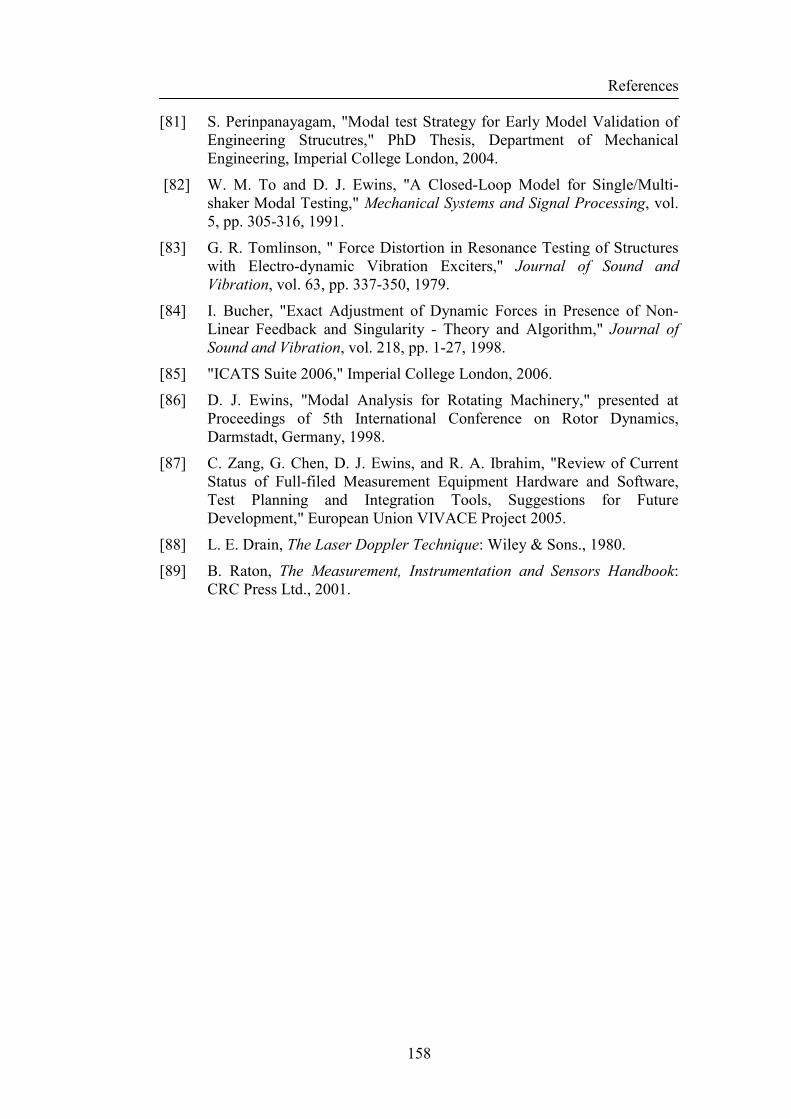
References
158
[81] S. Perinpanayagam, "Modal test Strategy for Early Model Validation of
Engineering Strucutres," PhD Thesis, Department of Mechanical
Engineering, Imperial College London, 2004.
[82] W. M. To and D. J. Ewins, "A Closed-Loop Model for Single/Multi-
shaker Modal Testing," Mechanical Systems and Signal Processing, vol.
5, pp. 305-316, 1991.
[83] G. R. Tomlinson, " Force Distortion in Resonance Testing of Structures
with Electro-dynamic Vibration Exciters," Journal of Sound and
Vibration, vol. 63, pp. 337-350, 1979.
[84] I. Bucher, "Exact Adjustment of Dynamic Forces in Presence of Non-
Linear Feedback and Singularity - Theory and Algorithm," Journal of
Sound and Vibration, vol. 218, pp. 1-27, 1998.
[85] "ICATS Suite 2006," Imperial College London, 2006.
[86] D. J. Ewins, "Modal Analysis for Rotating Machinery," presented at
Proceedings of 5th International Conference on Rotor Dynamics,
Darmstadt, Germany, 1998.
[87] C. Zang, G. Chen, D. J. Ewins, and R. A. Ibrahim, "Review of Current
Status of Full-filed Measurement Equipment Hardware and Software,
Test Planning and Integration Tools, Suggestions for Future
Development," European Union VIVACE Project 2005.
[88] L. E. Drain, The Laser Doppler Technique: Wiley & Sons., 1980.
[89] B. Raton, The Measurement, Instrumentation and Sensors Handbook:
CRC Press Ltd., 2001.

Appendix A Technical Drawings
159
Appendix A
Technical Drawings
A.1 Casing
A.2 Linear Bearing Support
A.3 Nonlinear Bearing Support – Rim
A.4 Nonlinear Bearing Support – Assembly
A.5 Shaft Lock
A.6 Rotor
A.7 Structural Bar and Miscellaneous Components

Appendix A Technical Drawings
160
A.1 Casing

Appendix A Technical Drawings
161
A.2 Linear Bearing Support
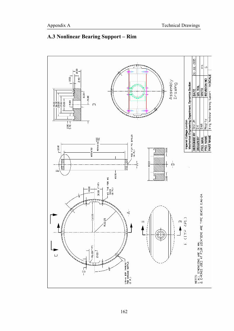
Appendix A Technical Drawings
162
A.3 Nonlinear Bearing Support – Rim
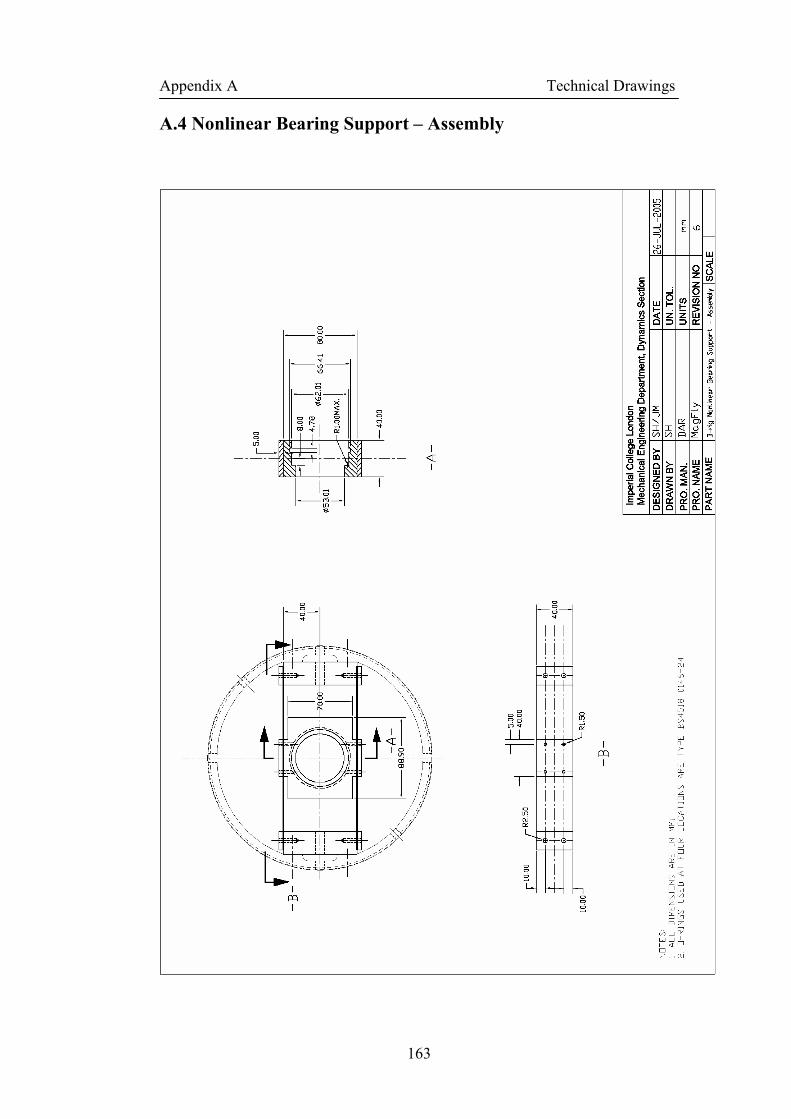
Appendix A Technical Drawings
163
A.4 Nonlinear Bearing Support – Assembly

Appendix A Technical Drawings
164
A.5 Shaft Lock
Appendix A Technical Drawings
165
A.6 Rotor
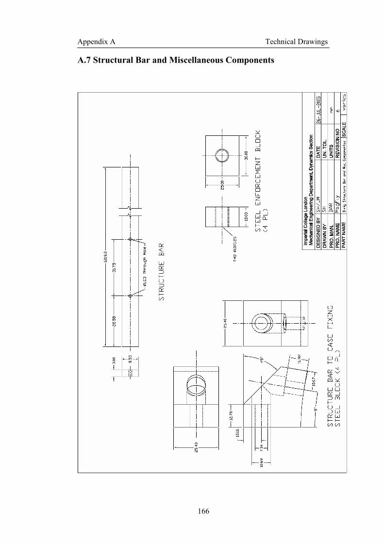
Appendix A Technical Drawings
166
A.7 Structural Bar and Miscellaneous Components
Appendix B Simulation of a 1-DOF Nonlinear Oscillator
167
Appendix B
Simulation of a 1-DOF Nonlinear
Oscillator
B.1 Comparison of results from time integration and HBM
calculation
The Nonlinear Bearing Support of the test rig was designed in such a way that it
displays in the horizontal direction a stiffness pattern that is the combination of a
negative linear stiffness and a third-order polynomial stiffness. The resultant
system governing equation is:
( ) ( ) ( ) ( ) ( )3
1 3 sinmu t cu t k u t k u t F tω+ + + =ɺɺ ɺ (B.1)
in which 1 0k < and 3 0k > .
Such equation also appears in population dynamics and Earth’s magnetic field
model. It was first systematically reported by Holmes [65] in 1979, and has since
become an interesting subject, mainly for mathematicians to understand the
intricate behaviours of such a nonlinear system. It is understood that multiple
steady-state solutions exist in a nonlinear system when it is under periodic
excitation. It will be very interesting to see how such kind of nonlinear responses
can be captured by frequency-domain calculations. It has been proven from this
exercise that HBM can locate steady-state solutions much faster than time-
domain method.
The following parameters are chosen for numerical studies: F =2000N; m =1kg;
c =1Ns/m; 1k =-1000N/m 3k =10000 N/m3. One of the main purposes of this

Appendix B Simulation of a 1-DOF Nonlinear Oscillator
168
study is to find as many as possible steady-state periodic solutions at any given
excitation frequency. Time-domain calculation based on Runge-Kutta method
was conducted at 24.6Hz. 200 different initial conditions, in terms of velocity
and displacement, were applied. Different types of steady-state solutions were
observed, manifested in the form of major- and sub- harmonic responses. HBM
was applied to the same system at the same excitation frequency. The
comparison of some of the steady-state responses are presented in Figure B - 1 to
Figure B - 6. The first plot shows the time domain variation of the response and
excitation, from which it is possible to judge what is the dominant harmonic
term in the response. The second plot is the so-called ‘phase diagram’ in which a
trajectory of motion is plotted over period of the response. The velocity and
displacement are the two coordinates.
325 325.05 325.1 325.15 -2 -1.5 -1
-0.5 0
0.5 1
1.5 2
Response Displacement (m
)
time (Sec) 325 325.05 325.1 325.15
-2000
-1000
0
1000
2000
Excitation Force (N)
-2 -1.5 -1 -0.5 0 0.5 1 1.5 2 -250 -200 -150 -100 -50 0 50 100 150 200 250
Displacement (m)
Velocity (m/s)
(a) (b)
Figure B - 1 (a)Time domain variation of displacement and excitation and (b) phase space
trajectory of solution of the major harmonic response with zero constant component in
(‘-·-·-·-’ external excitation, ‘___‘ time integration, ‘········ ‘ one harmonic term (1) included,
‘-∆--∆--∆--‘ two harmonic (1, 3) terms included.)
325 325.05 325.1 325.15 325.2 325.25 -0.5 -0.4 -0.3 -0.2 -0.1 0
0.1 0.2 0.3 0.4 0.5
Response Displacement (m
)
time (Sec) 325 325.05 325.1 325.15 325.2 325.25
-2000
-1000
0
1000
2000
Excitation Force (N)
-0.4 -0.3 -0.2 -0.1 0 0.1 0.2 0.3 0.4 -15 -10 -5 0 5 10 15
Displacement (m)
Velocity (m/s)
(a) (b)
Figure B - 2 (a) Time domain variation of displacement and excitation and (b) phase space
trajectory of solution of the major harmonic response with a constant component
(‘-·-·-·-’ external excitation, ‘___‘ time integration, ‘········ ‘ one harmonic (1) term included,
‘-∆--∆--∆--‘ three harmonic (0, 1, 2) terms included.)

Appendix B Simulation of a 1-DOF Nonlinear Oscillator
169
325 325.05 325.1 325.15 325.2 325.25 325.3
0
Response Displacement (m
)
time (Sec) 325 325.05 325.1 325.15 325.2 325.25 325.3
-2000
0
2000
Excitation Force (N)
-1.5 -1 -0.5 0 0.5 1-80 -60 -40 -20 0 20 40 60 80
Displacement (m)
Velocity (m/s)
(a) (b)
Figure B - 3 (a) Time domain variation of displacement and excitation and (b) phase space
trajectory of solution of 1/2 sub-harmonic response
(‘-·-·-·-’ external excitation, ‘___‘ time integration, ‘········ ‘ two harmonic terms (0, 1/2)
included, ‘-∆--∆--∆--‘ four harmonic (0, 1/2, 2/2, 3/2) terms included.)
325 325.05 325.1 325.15 325.2 325.25 -0.8 -0.6 -0.4 -0.2 0
0.2 0.4 0.6 0.8
Response Displacement (m
)
time (Sec) 325 325.05 325.1 325.15 325.2 325.25
-2000 -1500 -1000 -500 0 500 1000 1500 2000
Excitation Force (N)
400
-0.8 -0.6 -0.4 -0.2 0 0.2 0.4 0.6 0.8 -50 -40 -30 -20 -10 0 10 20 30 40 50
Velocity (m/s)
Displacement (m) (a) (b)
Figure B - 4 (a) Time domain variation of displacement and excitation and (b) phase space
trajectory of 1/3 sub-harmonic response
(‘-·-·-·-’ external excitation, ‘___‘ time integration, ‘········ ‘ one harmonic term (1/3)
included, ‘-∆--∆--∆--‘ two harmonic terms (1/3, 3/3) included.)
325 325.05 325.1 325.15 325.2 325.25 325.3 -0.5 -0.4 -0.3 -0.2 -0.1 0
0.1 0.2 0.3 0.4 0.5
Response Displacement (m
)
time (Sec) 325 325.05 325.1 325.15 325.2 325.25 325.3
-2000 -1500 -1000 -500 0 500 1000 1500 2000
Excitation Force (N)
-0.5 -0.4 -0.3 -0.2 -0.1 0 0.1 0.2 0.3 0.4 0.5-20 -15 -10 -5 0
5
10 15 20
Displacement (m)
Velocity (m/s)
(a) (b)
Figure B - 5 (a) Time domain variation of displacement and excitation and (b) phase space
trajectory of 1/4 sub-harmonic response
(‘-·-·-·-’ external excitation, ‘___‘ time integration, ‘········ ‘ two harmonic terms (0, ¼)
included, ‘-∆--∆--∆--‘ five harmonic terms (0, ¼, 2/4, ¾, 4/4) included.)
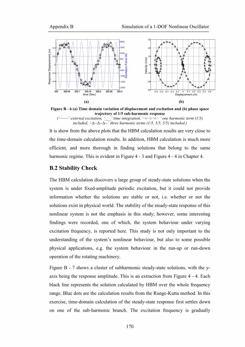
Appendix B Simulation of a 1-DOF Nonlinear Oscillator
170
325 325.05 325.1 325.15 325.2 325.25 325.3
-0.4 -0.2 0
0.2 0.4
Response Displacement (m
)
time (Sec) 325 325.05 325.1 325.15 325.2 325.25 325.3
-2000 -1500 -1000 -500 0 500 1000 1500 2000
Excitation Force (N)
-0.5 -0.4 -0.3 -0.2 -0.1 0 0.1 0.2 0.3 0.4 0.5 -30 -20 -10 0 10 20 30
Displacement (m)
Velocity (m/s)
(a) (b)
Figure B - 6 (a) Time domain variation of displacement and excitation and (b) phase space
trajectory of 1/5 sub-harmonic response
(‘-·-·-·-’ external excitation, ‘___‘ time integration, ‘········ ‘ one harmonic term (1/5)
included, ‘-∆--∆--∆--‘ three harmonic terms (1/5, 3/5, 5/5) included.)
It is show from the above plots that the HBM calculation results are very close to
the time-domain calculation results. In addition, HBM calculation is much more
efficient, and more thorough in finding solutions that belong to the same
harmonic regime. This is evident in Figure 4 - 3 and Figure 4 - 4 in Chapter 4.
B.2 Stability Check
The HBM calculation discovers a large group of steady-state solutions when the
system is under fixed-amplitude periodic excitation, but it could not provide
information whether the solutions are stable or not, i.e. whether or not the
solutions exist in physical world. The stability of the steady-state response of this
nonlinear system is not the emphasis in this study; however, some interesting
findings were recorded, one of which, the system behaviour under varying
excitation frequency, is reported here. This study is not only important to the
understanding of the system’s nonlinear behaviour, but also to some possible
physical applications, e.g. the system behaviour in the run-up or run-down
operation of the rotating machinery.
Figure B - 7 shows a cluster of subharmonic steady-state solutions, with the y-
axis being the response amplitude. This is an extraction from Figure 4 - 4. Each
black line represents the solution calculated by HBM over the whole frequency
range. Blue dots are the calculation results from the Runge-Kutta method. In this
exercise, time-domain calculation of the steady-state response first settles down
on one of the sub-harmonic branch. The excitation frequency is gradually
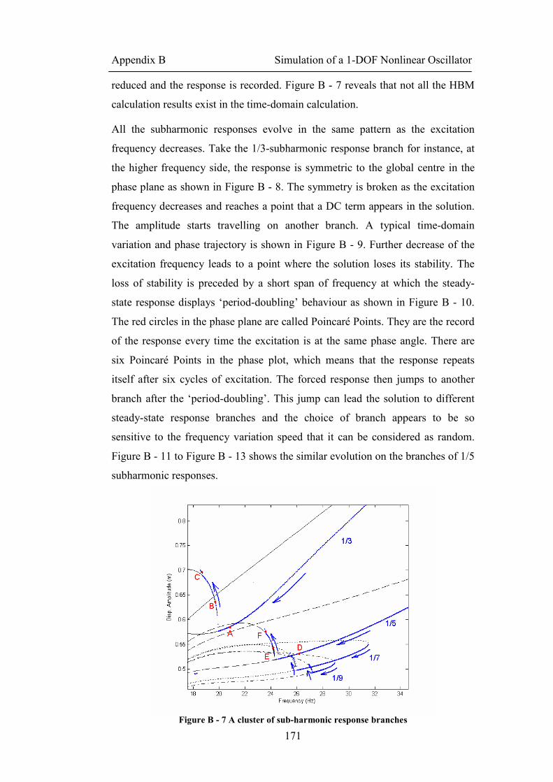
Appendix B Simulation of a 1-DOF Nonlinear Oscillator
171
reduced and the response is recorded. Figure B - 7 reveals that not all the HBM
calculation results exist in the time-domain calculation.
All the subharmonic responses evolve in the same pattern as the excitation
frequency decreases. Take the 1/3-subharmonic response branch for instance, at
the higher frequency side, the response is symmetric to the global centre in the
phase plane as shown in Figure B - 8. The symmetry is broken as the excitation
frequency decreases and reaches a point that a DC term appears in the solution.
The amplitude starts travelling on another branch. A typical time-domain
variation and phase trajectory is shown in Figure B - 9. Further decrease of the
excitation frequency leads to a point where the solution loses its stability. The
loss of stability is preceded by a short span of frequency at which the steady-
state response displays ‘period-doubling’ behaviour as shown in Figure B - 10.
The red circles in the phase plane are called Poincaré Points. They are the record
of the response every time the excitation is at the same phase angle. There are
six Poincaré Points in the phase plot, which means that the response repeats
itself after six cycles of excitation. The forced response then jumps to another
branch after the ‘period-doubling’. This jump can lead the solution to different
steady-state response branches and the choice of branch appears to be so
sensitive to the frequency variation speed that it can be considered as random.
Figure B - 11 to Figure B - 13 shows the similar evolution on the branches of 1/5
subharmonic responses.
Figure B - 7 A cluster of sub-harmonic response branches
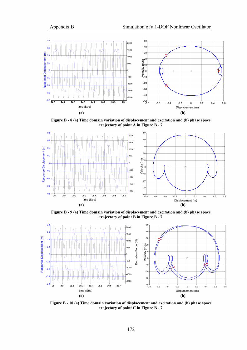
Appendix B Simulation of a 1-DOF Nonlinear Oscillator
172
(a) (b)
Figure B - 8 (a) Time domain variation of displacement and excitation and (b) phase space
trajectory of point A in Figure B - 7
(a) (b)
Figure B - 9 (a) Time domain variation of displacement and excitation and (b) phase space
trajectory of point B in Figure B - 7
(a) (b)
Figure B - 10 (a) Time domain variation of displacement and excitation and (b) phase space
trajectory of point C in Figure B - 7
-0.8 -0.6 -0.4 -0.2 0 0.2 0.4 0.6 0.8 -40
-30
-20
-10
0
10
20
30
40
50
Displacement (m)
Velocity (m/s)
26 26.1 26.2 26.3 26.4 26.5 26.6 26.7 -0.8
-0.6
-0.4
-0.2
0
0.2
0.4
0.6
0.8
Response Displacement (m
)
time (Sec)
26 26.1 26.2 26.3 26.4 26.5 26.6 26.7 -2000
-1500
-1000
-500
0
500
1000
1500
2000
Excitation Force (N)
25 25.1 25.2 25.3 25.4 25.5 25.6 25.7 -0.8
-0.6
-0.4
-0.2
0
0.2
0.4
0.6
0.8
Response Displacement (m
)
time (Sec)
25 25.1 25.2 25.3 25.4 25.5 25.6 25.7
-2000
-1500
-1000
-500
0
500
1000
1500
2000
24.3 24.4 24.5 24.6 24.7 24.8 24.9 25 -0.8
-0.6
-0.4
-0.2
0
0.2
0.4
0.6
0.8 Response Displacement (m
)
time (Sec)
24.3 24.4 24.5 24.6 24.7 24.8 24.9 25 -2000
-1500
-1000
-500
0
500
1000
1500
2000
Excitation Force (N)
-0.8 -0.6 -0.4 -0.2 0 0.2 0.4 0.6 -50
-40
-30
-20
-10
0
10
20
30
40
50
Velocity (m/s)
Displacement (m)
-0.8 -0.6 -0.4 -0.2 0 0.2 0.4 0.6 0.8 -40
-30
-20
-10
0
10
20
30
40
50
Displacement (m)
Velocity (m/s)
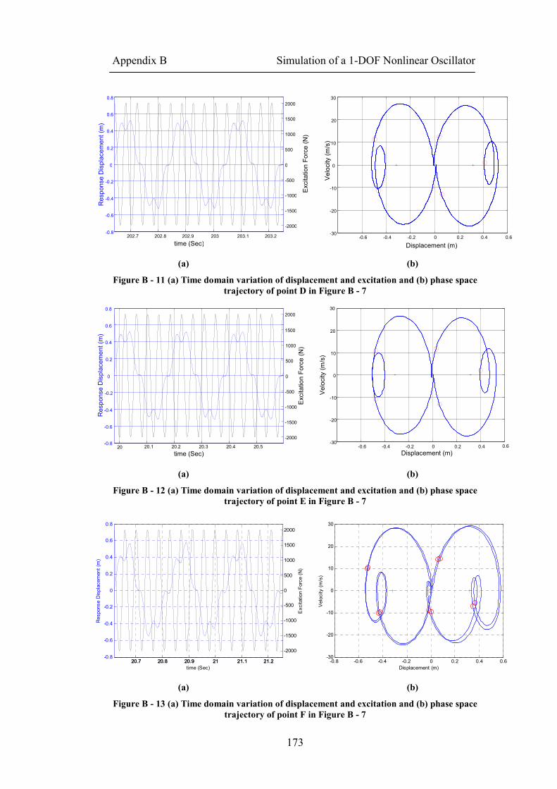
Appendix B Simulation of a 1-DOF Nonlinear Oscillator
173
(a) (b)
Figure B - 11 (a) Time domain variation of displacement and excitation and (b) phase space
trajectory of point D in Figure B - 7
(a) (b)
Figure B - 12 (a) Time domain variation of displacement and excitation and (b) phase space
trajectory of point E in Figure B - 7
(a) (b)
Figure B - 13 (a) Time domain variation of displacement and excitation and (b) phase space
trajectory of point F in Figure B - 7
-0.6 -0.4 -0.2 0 0.2 0.4 0.6 -30
-20
-10
0
10
20
30
Displacement (m)
Velocity (m/s)
202.7 202.8 202.9 203 203.1 203.2 -0.8
-0.6
-0.4
-0.2
0
0.2
0.4
0.6
0.8 Response Displacement (m
)
time (Sec)
-2000
-1500
-1000
-500
0
500
1000
1500
2000
Excitation Force (N)
-0.6 -0.4 -0.2 0 0.2 0.4 0.6 -30
-20
-10
0
10
20
30
Displacement (m)
Velocity (m/s)
20 20.1 20.2 20.3 20.4 20.5 -0.8
-0.6
-0.4
-0.2
0
0.2
0.4
0.6
0.8
Response Displacement (m
)
time (Sec)
-2000
-1500
-1000
-500
0
500
1000
1500
2000
Excitation Force (N)
20.7 20.8 20.9 21 21.1 21.2-0.8
-0.6
-0.4
-0.2
0
0.2
0.4
0.6
0.823.55
Response Displacement (m
)
time (Sec)
20.7 20.8 20.9 21 21.1 21.2
-2000
-1500
-1000
-500
0
500
1000
1500
2000
Excitation Force (N)
-0.8 -0.6 -0.4 -0.2 0 0.2 0.4 0.6-30
-20
-10
0
10
20
3023.55
Displacement (m)
Velocity (m/s)