dynamic allocation strategies for absolute and relative...
TRANSCRIPT
Dynamic Allocation Strategiesfor Absolute and Relative Loss Control
July 2014
Daniel Mantilla-GarcíaResearch Associate, EDHEC-Risk Institute Head of Research & Development, Koris International
2
AbstractThe maximum drawdown control strategy dynamically allocates wealth between cash and a risky portfolio, keeping losses below a chosen pre-defined level. This paper introduces variations of the strategy, namely the excess drawdown and the relative drawdown control strategies. The excess drawdown control is a more flexible strategy that can cope with common (re)allocation restrictions such as lock-up periods, cash bans or liquidity constraints through an implementation with a hedging overlay. The relative drawdown control strategy is adapted to contexts in which investors seek to limit benchmark underperformance instead of absolute losses. A formal proof that the loss-control objectives introduced can be insured using dynamic allocation is providedand the potential benefits and implementation aspects of the strategies are illustrated with examples.
Keywords: Risk Management, Portfolio Insurance, Hedging Overlay, Loss Aversion, Benchmarks.JEL classification: G11, G110.
The author would like to thank Maxime Bonelli, Marco Leoni and two anonymous referees for many detailed remarks and suggestions and Emilien Audeguil, Arnaud Izard, Lionel Martellini, Raman Uppal and Koris International team for valuable comments and discussions. Financial support from Koris International is gratefully acknowledged.
EDHEC is one of the top five business schools in France. Its reputation is built on the high quality of its faculty and the privileged relationship with professionals that the school has cultivated since its establishment in 1906. EDHEC Business School has decided to draw on its extensive knowledge of the professional environment and has therefore focused its research on themes that satisfy the needs of professionals.
EDHEC pursues an active research policy in the field of finance. EDHEC-Risk Institute carries out numerous research programmes in the areas of asset allocation and risk management in both the traditional and alternative investment universes.
Copyright © 2014 EDHEC
3
1 - Other investment strategies using drawdowns as the risk metric of concern include Carr, Zhang, and Hadjiliadis (2011), Zhang, Leung, and Hadjiliadis (2013), and Chekhlov, Uryasev, and Zabarankin (2000,2005). Portfolio sensitivities to max drawdown are studied in Pospisil and Vecer (2010) and probabilistic properties of drawdowns in Douady, Shiryaev, and Yor (2000), Magdon-Ismail, Atiya, Pratap, and Abu- Mostafa (2004), Pospisil and Vecer (2008), Hadjiliadis and Vecer (2006), Pospisil, Vecer, and Hadjiliadis (2009), Zhang and Hadjiliadis (2010, 2012), and Zhang (2014).2 - Other studies on the optimality of the drawdown control strategy are Elie and Touzi (2008) (case with intermediate consumption), Kim (2011), and Roche (2013).3 - Sometimes we refer to the standard drawdowns as “absolute losses”, in contrast to the “relative losses” measured by the relative drawdowns. 4 - Not to be confused with the standard maximum drawdown (MDD) concept, which is sometimes called relative MDD to differentiate it from its version expressed in dollar terms as opposed to relative change terms (returns). In this article we always work with drawdowns expressed as returns.
1 IntroductionInvestment strategies controlling drawdowns (cumulative losses over intermediate horizons) are popular in investment management. Empirical observations show that funds yielding overly poor performance often face significant withdrawal/redemption, or liquidation, leading managers to decrease leverage following poor performance to increase the fund’s survival likelihood (see Ang, Gorovyy, and Van Inwegen, 2011; Patton and Ramadorai, 2013). Furthermore, the optimal strategy of a fund manager compensated with common high-water-mark based performance fees can integrate a drawdown control motive1 (see Drechsler, 2014; Guasoni and Obloj, 2011; Goetzmann, Ingersoll, and Ross, 2003; Pangeas and Westerfield, 2009; Lan, Wang, and Yang, 2013).
The Time-Invariant Portfolio Protection (TIPP) or maximum drawdown control strategy was introduced by Estep and Kritzman (1988), and Grossman and Zhou (1993) showed that the strategy can be utility maximising under the max drawdown constraint. Cvitanic and Karatzas (1995) generalised the optimal solution for the case with multiple risky assets with more general dynamics and a stochastic short-term interest rate.2 Following a dynamic allocation rule between cash and a performance-seeking asset, the strategy limits the portfolio’s maximum drawdown to a given tolerance level set ex-ante. However, this dynamic allocation rule is often at odds with other objectives and practical considerations of investors and managers, depending on the context. First, some assets liquidity often dries up precisely during important drawdown periods, posing an implementation burden to the standard drawdown control strategy, particularly for large institutional investors. Second, active investment funds often impose mechanisms to dissuade or withhold investors from selling their shares after large fund losses (as the drawdown control strategy would do), to prevent the fund from selling assets when prices are presumably low and realising losses to remaining investors. Third, holding a large proportion of cash is inconvenient or even contractually banned for some professional investment managers, due to the associated opportunity cost that increases with loss aversion and lower interest rates. Fourth, holding an important share of cash with the purpose of controlling short-term losses can conflict with other risk-management objectives, such as hedging long-term liabilities.
This paper introduces a variation of the drawdown control strategy compatible with the need or will to avoid using cash as the reserve asset and with common reallocation or liquidity restrictions. The strategy controls the drawdown in excess of the drawdown experienced by a given reserve asset, the latter being any chosen safe enough asset. Furthermore, in presence of reallocation restrictions, a drawdown control can be implemented through a hedging overlay (see Healy and Lo, 2009). Hedging overlay strategies are subject to basis risk, arising from an imperfect correlation between the hedging instrument(s) and the assets in the portfolio. While in presence of basis risk the standard drawdown control strategy cannot be effectively implemented with a hedging overlay as it would cause violations of its constraint, the excess drawdown control strategy can directly incorporate basis risk, allowing investors to limit drawdowns in excess of the losses caused by hedging imperfections. In other words, the excess drawdown strategy implemented with a hedging overlay controls the hedgeable proportion of the portfolio drawdowns. This is of particular interest for large institutional investors trying to avoid a potential (adverse) impact on market prices of their assets reallocations during liquidity stress periods, which often coincide with large drawdown periods, or for investors seeking to limit the drawdowns of portfolios invested in assets with limited liquidity.
This paper also discusses how the risk-metric and drawdown-control strategy can be adapted to a relative performance context in which the objective is to control the underperformance of a given (investable) benchmark instead of absolute losses.3 We introduce the concept of relative drawdown,4 which is a measure of maximum cumulative underperformance with respect to a

4
given benchmark, as well as the dynamic allocation strategy to control this relative risk. Unlike (excess) absolute drawdowns, relative drawdowns may happen during ‘bull markets’. The strategy can be of particular interest for investors entering ‘alternative betas’ and/or active investment funds, for which the expected outperformance usually comes with an important benchmark underperformance risk.
Hereafter we also show that these dynamic allocation strategies can be modified to control excess drawdowns and relative drawdowns measured over a rolling period of time as opposed to since inception, which increases their exposure to the performance-seeking assets. In empirical tests we find that the introduction of a rolling period in the performance constraints induces an improvement in terms of risk-adjusted performance.
In this paper we present a formal proof that the Floors and risk-management constraints introduced can be insured using standard dynamic asset allocation-based portfolio insurance strategies. Furthermore, we also provide an estimate of the discrete-time trading of the upper bounds of the multiplier of these kinds of strategies. Such upper bounds are also useful for the implementation of strategies similar to the Constant Proportion Portfolio Insurance (CPPI) (Perold, 1986; Black and Jones, 1987; Black and Perold, 1992) in their general case with a locally risky reserve asset (see for instance Amenc, Malaise, and Martellini, 2004; Mantilla- García, 2014). An important characteristic of the drawdown control strategies treated here is that they insure their risk-management objectives for investors entering into the strategy at any point in time. Thus, unlike other portfolio insurance strategies such as CPPI and the Dynamic Core-Satellite in Amenc et al. (2004, which provide protection to investors entering the strategy at initial date only, they are adapted for implementation to open funds.
2. Dynamic Allocation Based Portfolio InsuranceThe aim of risk-control allocation strategies such as CPPI and the maximum drawdown control strategy (i.e. TIPP) is to insure that the portfolio respects a given performance constraint that represents the risk-management objective of the investor.5 Such strategies achieve so through a dynamic asset allocation rule that prevents the value of the portfolio, denoted A, to fall below a Floor value F. These kinds of strategies split wealth between a risky, performance-seeking asset S, and a reserve or safe asset, B. The allocation rule consists of maintaining at every time t a proportion of wealth invested in asset S equal to
(1)
and the remaining wealth invested in the reserve asset B, where the multiplier mt ≥ 0 is a constant or an adapted time-varying process. Whenever A approaches F, wealth is reallocated towards the reserve asset to prevent the portfolio from breaching its Floor value.
Obviously, not all kinds of Floor processes can be insured using a type (1) dynamic allocation strategy. Hence, in order to define a type (1) strategy that can insure a given performance constraint, one needs to i) define the Floor process, ii) prove that if A(t) ≥ F(t) for all t then A satisfies the given performance constraint, and iii) prove that the Floor is insurable. A Floor process F of a type (1) strategy A is insurable, if it can be shown that under certain conditions A(t) ≥ F(t) for all t. This paper achieves these three objectives for the excess drawdown and relative drawdown constraints and the corresponding strategies introduced.
While the allocation of type (1) strategies changes continuously over time in theory, trading only happens in discrete time. Hence, in order to set weights back to the current target, reallocations are triggered whenever the actual portfolio exposure and its target drift apart beyond a given
5 - Browne (1999), Browne (2000), and Basak, Shapiro, and Teplá (2006) study other kind of risk-control strategies in which the investor does not abide the kind of hard constraints of portfolio insurance strategies, but rather make sure that the probability of violating the (relative) performance constraint(s) by a margin error of size ε does not exceed a given probability.
percentage. More precisely, let the implied multiplier of type (1) strategies be defined as
where . No trading takes place whenever and reallocations are triggered every time exits the no-trading band. In our illustrations below, we set τ = 0.2 as in Hamidi, Maillet, and Prigent (2012), which yields reasonable reallocation frequency and turnover figures, and we enforce a no-leverage type upper bound on ωS(t) i.e.,
.
An important issue regards the determination of the multiplier. Optimal multipliers for the CPPI (Black and Perold, 1992; Grossman and Vila, 1992; Mantilla-García, 2014) or TIPP (Grossman and Zhou, 1993; Cvitanic and Karatzas, 1995) are a function of the expected excess return of assets. In practice, risk-based asset allocation programs independent from expected return estimates have become increasingly popular. For instance, in the CPPI literature the multiplier is often set close to its upper bound or maximal multiplier, that is, the maximum multiplier value that would allow the strategy to respect its performance constraint and Floor for a given confidence level, when trading happens in discrete time and/or asset prices “jump”. In former papers, the maximal multiplier is usually estimated as the inverse of the expected shortfall of the risky asset over one day. For stock prices, the size of expected returns over short horizons, such as one day, are negligible compared to the size of large percentiles of the return distribution. Thus, in that case, one can safely assume expected returns are equal to zero in estimating the expected shortfall, which means that the maximal multiplier implies a risk-based asset allocation program not dependent on expected return estimates. Studies on the maximum risk-based multiplier such as Bertrand and Prigent (2002), Cont and Tankov (2009), and Hamidi, Maillet, and Prigent (2014), assume that B is a locally riskless asset paying a constant rate of return considered “relatively small” compared to the worst possible loss in the risky asset. However, when the reservasset B is locally risky (as in the strategies considered here and the more general version of the CPPI discussed in Mantilla-García (2014)), the right tail of the return distribution of B also becomes relevant to estimate the upper bound of the multiplier. In Appendix A we show that a conservative risk-based estimate of the upper bound of the multiplier for the strategies studied here is, (2)
where LTS(t, h) and RTB(t, h) correspond to the left and right tails estimates of the return distributions of assets S and B respectively over a horizon of h periods. The horizon h corresponds to the maximum period of time the manager may require to effectively reallocate assets once the reallocation is triggered. In the illustrations in this paper, reallocations are implemented on t + 2, where t corresponds to the day when the reallocation is triggered and the multiplier estimation date. For this reason, in our illustrations we use conditional estimates of the Expected Shortfall (ES) of RS and of −RB over a horizon of 2 days with a 99.99% confidence level as the left and right tails estimates respectively. We follow the McNeil and Frey (2000) methodology to estimate the conditional ES of RS and −RB. The approach combines a GARCH model (see Engle, 2001) to filter the volatility of returns and an extreme value theory distribution to model the tails of GARCH residuals. This method has the advantages of being somewhat agnostic about the distribution of returns while taking into account their natural fat tails and heteroscedasticity.
Although the CPPI and the TIPP are both type (1) strategies, they have very distinct behaviours because their Floor formulas, and thus the risk-management constraints they serve are very different. Indeed, while the TIPP limits losses incurred over any intermediate horizon, the CPPI strategy only limits the losses experienced by the portfolio as measured with respect to the initial date. As a consequence, the TIPP can guarantee its risk-management objective to investors
5

6
entering into an investment fund at any point in time, while CPPI only offers its guarantee to investors entering the strategy at the initial date.6
Let t0 denote the initial investment date, unless otherwise stated and the information set available at time t, including past values of A, B and S. The maximum drawdown (MDD) of an investment is defined as the largest value loss from a peak to a bottom observed at current time t. More precisely, for a value process A, the drawdown at time s, denoted Ds(A), is the percentage loss experienced by A with respect to its running maximum observed since time t0, denoted , attained for the last time at . Therefore, the maximum drawdown observed since inception t0 = 0 to current time t , denoted by , is defined as follows:
(3)
(4)
(5)
(6)
where RA(t1, t2) denotes the simple return of A between the two instants t1 ≤ t2, and the drawdown period of Ds(A) is . The maximum drawdown constraint on portfolio A is (7)
where the risk budget x ∈ (0, 1), represents the maximum percentage loss on current capital that the investor is willing to tolerate at any point in time. As aforementioned, the objective of the portfolio insurance strategies discussed in this paper is to insure a risk-management performance constraint such as (7) using dynamic allocation.
For the MDD strategy, the Floor value is defined at every time t as follows (8)
where k := (1 − x). If the value of the portfolio is always above the MDD Floor (8), then constraint (7) is respected, since the following statements are equivalent, (9)
(10)
for all s ∈[t0, t] and t ∈[s, ∞). Notice that the MDD Floor (8) is a strictly non-decreasing function of time. Consequently for the MDD Floor to be insurable, the reserve asset must be an asset with a strictly positive performance at all times to (super-)replicate the Floor during drawdown periods; hence bounded to be cash. Grossman and Zhou (1993) and Cvitanic and Karatzas (1995) consider a similar strategy for which the drawdown and the corresponding Floor are defined in terms of a high water mark (HWM) or discounted wealth process. In that case, the Floor value is
(11)
where S0 is a discount value process growing at rate r (e.g. a savings account paying a short-term interest rate). This Floor presents a more binding constraint than (8), since the HWM grows exponentially at the short-term rate instead of being flat during drawdown periods of A. Lan et al. (2013) and Goetzmann et al. (2003) point out that the fund’s HWM should be adjusted downward when money flows out of the fund due to management fees or if investors continuously redeem capital at a consumption rate y. Hence the HWM grows at the rate r − y and for y = r, the
6 - In effect, the CPPI can present severe cumulative losses over arbitrarily long intermediate horizons, as the portfolio loses former cumulated capital gains during drawdown periods of the risky asset.
7 - While the TIPP exposure reaches an upper bound every time the value of the portfolio attains a new maximum, the CPPI’s risk exposure grows exponentially during ‘bull’ markets and remains theoretically unlimited.8 - From there on, we refer sometimes to the maximum drawdown as the “global MDD”, and to the maximum drawdown with a restricted calculation horizon as the “rolling MDD”.
7
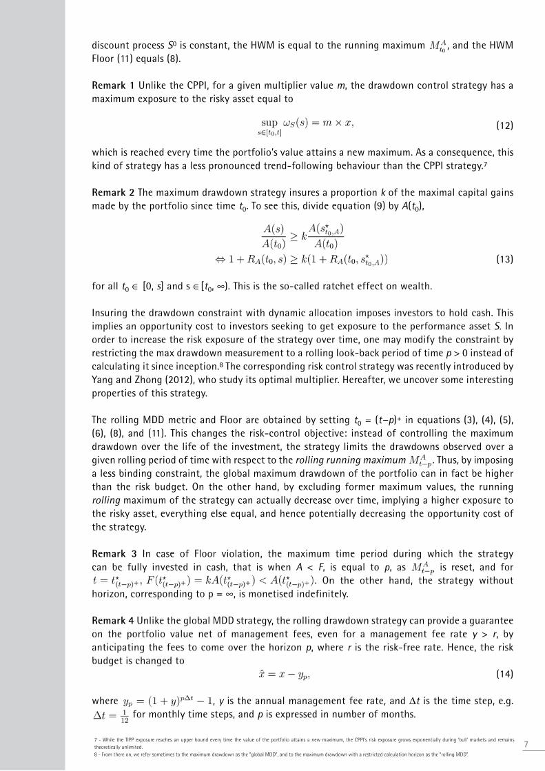
discount process S0 is constant, the HWM is equal to the running maximum , and the HWM Floor (11) equals (8).
Remark 1 Unlike the CPPI, for a given multiplier value m, the drawdown control strategy has a maximum exposure to the risky asset equal to
(12)
which is reached every time the portfolio’s value attains a new maximum. As a consequence, this kind of strategy has a less pronounced trend-following behaviour than the CPPI strategy.7
Remark 2 The maximum drawdown strategy insures a proportion k of the maximal capital gains made by the portfolio since time t0. To see this, divide equation (9) by A(t0),
(13)
for all t0 ∈ [0, s] and s ∈[t0, ∞). This is the so-called ratchet effect on wealth.
Insuring the drawdown constraint with dynamic allocation imposes investors to hold cash. This implies an opportunity cost to investors seeking to get exposure to the performance asset S. In order to increase the risk exposure of the strategy over time, one may modify the constraint by restricting the max drawdown measurement to a rolling look-back period of time p > 0 instead of calculating it since inception.8 The corresponding risk control strategy was recently introduced by Yang and Zhong (2012), who study its optimal multiplier. Hereafter, we uncover some interesting properties of this strategy.
The rolling MDD metric and Floor are obtained by setting t0 = (t−p)+ in equations (3), (4), (5), (6), (8), and (11). This changes the risk-control objective: instead of controlling the maximum drawdown over the life of the investment, the strategy limits the drawdowns observed over a given rolling period of time with respect to the rolling running maximum . Thus, by imposing a less binding constraint, the global maximum drawdown of the portfolio can in fact be higher than the risk budget. On the other hand, by excluding former maximum values, the running rolling maximum of the strategy can actually decrease over time, implying a higher exposure to the risky asset, everything else equal, and hence potentially decreasing the opportunity cost of the strategy.
Remark 3 In case of Floor violation, the maximum time period during which the strategy can be fully invested in cash, that is when A < F, is equal to p, as is reset, and for
. On the other hand, the strategy without horizon, corresponding to p = ∞, is monetised indefinitely.
Remark 4 Unlike the global MDD strategy, the rolling drawdown strategy can provide a guarantee on the portfolio value net of management fees, even for a management fee rate y > r, by anticipating the fees to come over the horizon p, where r is the risk-free rate. Hence, the risk budget is changed to (14)
where , y is the annual management fee rate, and Δt is the time step, e.g. for monthly time steps, and p is expressed in number of months.
7
8
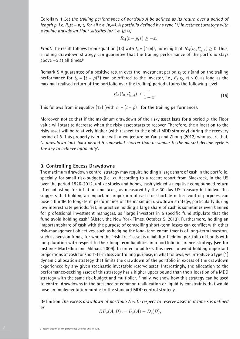
Corollary 1 Let the trailing performance of portfolio A be defined as its return over a period of length p, i.e. RA(t − p, t) for all t ∈ [p,∞). A portfolio defined by a type (1) investment strategy with a rolling drawdown Floor satisfies for t ∈ [p,∞)
Proof. The result follows from equation (13) with t0 = (t−p)+, noticing that . Thus, a rolling drawdown strategy can guarantee that the trailing performance of the portfolio stays above −x at all times.9
Remark 5 A guarantee of a positive return over the investment period t0 to t (and on the trailing performance for t0 = (t − p)+) can be offered to the investor, i.e., RA(t0, t) > 0, as long as the maximal realised return of the portfolio over the (rolling) period attains the following level:
(15)
This follows from inequality (13) (with t0 = (t − p)+ for the trailing performance).
Moreover, notice that if the maximum drawdown of the risky asset lasts for a period p, the Floor value will start to decrease when the risky asset starts to recover. Therefore, the allocation to the risky asset will be relatively higher (with respect to the global MDD strategy) during the recovery period of S. This property is in line with a conjecture by Yang and Zhong (2012) who assert that, “a drawdown look-back period H somewhat shorter than or similar to the market decline cycle is the key to achieve optimality”.
3. Controlling Excess DrawdownsThe maximum drawdown control strategy may require holding a large share of cash in the portfolio, specially for small risk-budgets (i.e. x). According to a recent report from Blackrock, in the US over the period 1926-2012, unlike stocks and bonds, cash yielded a negative compounded return after adjusting for inflation and taxes, as measured by the 30-day US Treasury bill index. This suggests that holding an important proportion of cash for short-term loss control purposes can pose a hurdle to long-term performance of the maximum drawdown strategy, particularly during low interest rate periods. Yet, in practice holding a large share of cash is sometimes even banned for professional investment managers, as “large investors in a specific fund stipulate that the fund avoid holding cash” (Alster, the New York Times, October 5, 2013). Furthermore, holding an important share of cash with the purpose of controlling short-term losses can conflict with other risk-management objectives, such as hedging the long-term commitments of long-term investors, such as pension funds, for whom the “risk-free” asset is a liability-hedging portfolio of bonds with long duration with respect to their long-term liabilities in a portfolio insurance strategy (see for instance Martellini and Milhau, 2009). In order to address this need to avoid holding important proportions of cash for short-term loss controlling purpose, in what follows, we introduce a type (1) dynamic allocation strategy that limits the drawdown of the portfolio in excess of the drawdown experienced by any given stochastic investable reserve asset. Interestingly, the allocation to the performance-seeking asset of this strategy has a higher upper bound than the allocation of a MDD strategy with the same risk budget and multiplier. Finally, we show how this strategy can be used to control drawdowns in the presence of common reallocation or liquidity constraints that would pose an implementation hurdle to the standard MDD control strategy.
Definition The excess drawdown of portfolio A with respect to reserve asset B at time s is defined as
9 - Notice that the trailing performance is defined only for t ≥ p.
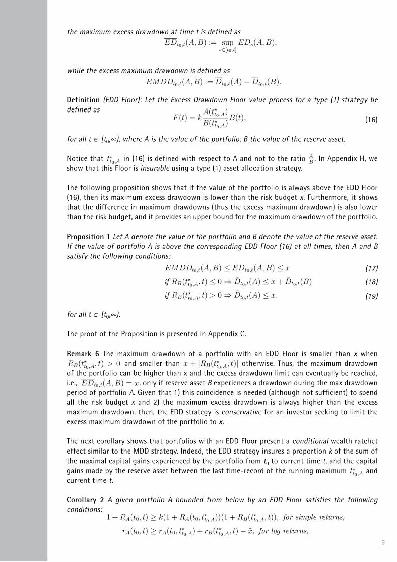
the maximum excess drawdown at time t is defined as
while the excess maximum drawdown is defined as
Definition (EDD Floor): Let the Excess Drawdown Floor value process for a type (1) strategy be defined as (16)
for all t ∈ [t0,∞), where A is the value of the portfolio, B the value of the reserve asset.
Notice that in (16) is defined with respect to A and not to the ratio . In Appendix H, we show that this Floor is insurable using a type (1) asset allocation strategy.
The following proposition shows that if the value of the portfolio is always above the EDD Floor (16), then its maximum excess drawdown is lower than the risk budget x. Furthermore, it shows that the difference in maximum drawdowns (thus the excess maximum drawdown) is also lower than the risk budget, and it provides an upper bound for the maximum drawdown of the portfolio.
Proposition 1 Let A denote the value of the portfolio and B denote the value of the reserve asset. If the value of portfolio A is above the corresponding EDD Floor (16) at all times, then A and B satisfy the following conditions: (17)
(18)
(19)
for all t ∈ [t0,∞).
The proof of the Proposition is presented in Appendix C.
Remark 6 The maximum drawdown of a portfolio with an EDD Floor is smaller than x when and smaller than otherwise. Thus, the maximum drawdown
of the portfolio can be higher than x and the excess drawdown limit can eventually be reached, i.e., , only if reserve asset B experiences a drawdown during the max drawdown period of portfolio A. Given that 1) this coincidence is needed (although not sufficient) to spend all the risk budget x and 2) the maximum excess drawdown is always higher than the excess maximum drawdown, then, the EDD strategy is conservative for an investor seeking to limit the excess maximum drawdown of the portfolio to x.
The next corollary shows that portfolios with an EDD Floor present a conditional wealth ratchet effect similar to the MDD strategy. Indeed, the EDD strategy insures a proportion k of the sum of the maximal capital gains experienced by the portfolio from t0 to current time t, and the capital gains made by the reserve asset between the last time-record of the running maximum and current time t.
Corollary 2 A given portfolio A bounded from below by an EDD Floor satisfies the following conditions:
9
10
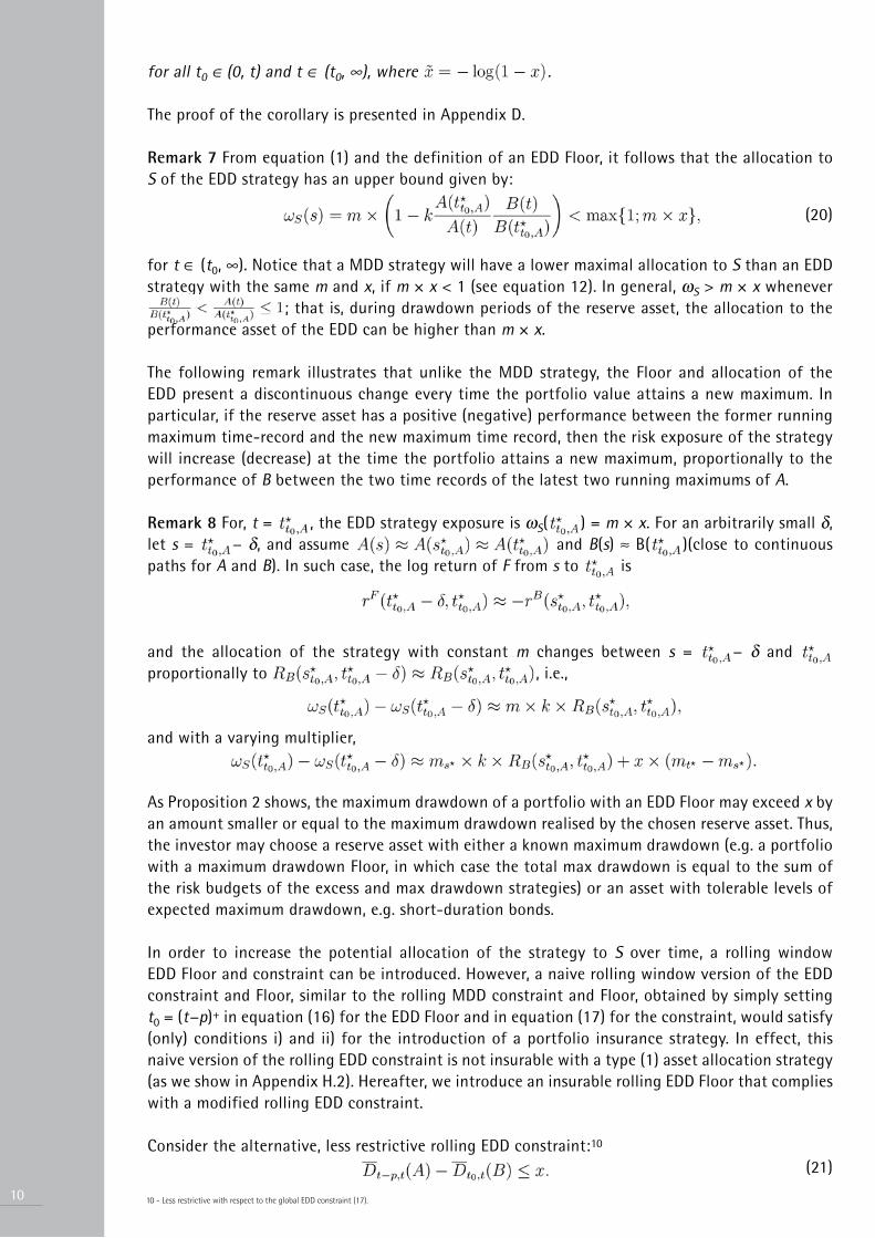
for all t0 ∈ (0, t) and t ∈ (t0, ∞), where .
The proof of the corollary is presented in Appendix D.
Remark 7 From equation (1) and the definition of an EDD Floor, it follows that the allocation to S of the EDD strategy has an upper bound given by:
(20)
for t ∈ (t0, ∞). Notice that a MDD strategy will have a lower maximal allocation to S than an EDD strategy with the same m and x, if m × x < 1 (see equation 12). In general, ωS > m × x whenever
; that is, during drawdown periods of the reserve asset, the allocation to the performance asset of the EDD can be higher than m × x.
The following remark illustrates that unlike the MDD strategy, the Floor and allocation of the EDD present a discontinuous change every time the portfolio value attains a new maximum. In particular, if the reserve asset has a positive (negative) performance between the former running maximum time-record and the new maximum time record, then the risk exposure of the strategy will increase (decrease) at the time the portfolio attains a new maximum, proportionally to the performance of B between the two time records of the latest two running maximums of A.
Remark 8 For, t = , the EDD strategy exposure is ωS( ) = m × x. For an arbitrarily small δ, let s = − δ, and assume and B(s) ≈ B( )(close to continuous paths for A and B). In such case, the log return of F from s to is
and the allocation of the strategy with constant m changes between s = − δ and proportionally to , i.e.,
and with a varying multiplier,
As Proposition 2 shows, the maximum drawdown of a portfolio with an EDD Floor may exceed x by an amount smaller or equal to the maximum drawdown realised by the chosen reserve asset. Thus, the investor may choose a reserve asset with either a known maximum drawdown (e.g. a portfolio with a maximum drawdown Floor, in which case the total max drawdown is equal to the sum of the risk budgets of the excess and max drawdown strategies) or an asset with tolerable levels of expected maximum drawdown, e.g. short-duration bonds.
In order to increase the potential allocation of the strategy to S over time, a rolling window EDD Floor and constraint can be introduced. However, a naive rolling window version of the EDD constraint and Floor, similar to the rolling MDD constraint and Floor, obtained by simply setting t0 = (t−p)+ in equation (16) for the EDD Floor and in equation (17) for the constraint, would satisfy (only) conditions i) and ii) for the introduction of a portfolio insurance strategy. In effect, this naive version of the rolling EDD constraint is not insurable with a type (1) asset allocation strategy (as we show in Appendix H.2). Hereafter, we introduce an insurable rolling EDD Floor that complies with a modified rolling EDD constraint.
Consider the alternative, less restrictive rolling EDD constraint:10
(21)
10 - Less restrictive with respect to the global EDD constraint (17).
Definition Let the conditional rolling maximum time process be defined as
(22)
where
(23)
and a rolling period p > 0, for all t ∈ [t0,∞), where Z := .
Definition (Rolling EDD Floor): Let the Rolling Excess Drawdown Floor value process for a type (1) strategy, and rolling period p, be defined as
(24)
for all t ∈ [t0, ∞), where A is the value of the portfolio, B the value of the reserve asset.
The definition of the rolling EDD is thus similar to its naive version, with the exception that its reference time for the running maximum of A rolls forward unless the current rolling running maximum decreased and the condition defining the set (23) is satisfied. In effect, the conditional running maximum time process of the rolling EDD Floor given by (24) only rolls forward at times in which the insurability of the Floor cannot be violated (see details in Appendix H.2).
Proposition 2 Let A denote the value of the portfolio and B denote the value of the reserve asset. If the value of portfolio A is above its rolling EDD Floor (24) at all times, then A and B satisfy the following conditions:
(25) (26)
(27)
for all t ∈ [t0, ∞).
The proof of the Proposition is presented in Appendix E.
Notice that the rolling EDD constraint (21) is equivalent to (25). Thus, the rolling EDD Floor (24) is less conservative than the global EDD Floor, in the sense that it insures a less binding performance constraint and thus a higher expected allocation to S over time, everything else being equal.
Drawdown control with a hedging overlayIn practice investors sometimes face reallocation constraints, which represent a burden for the implementation of type (1) dynamic allocation strategies. Such reallocation constraints come for instance in the form of lock-up periods or assets illiquidity.
Healy and Lo (2009) provided a detailed explanation of the logic and implementation of a “beta repositioning” program, which consists in modifying the risk exposure of a portfolio by taking a countervailing position in a hedging overlay portfolio through leverage, instead of disinvesting from the risky assets. The hedging overlay is composed by liquid instruments such as futures or forward contracts presenting an important correlation with the risky assets in the portfolio.
11

12
Consider the simplest case in which a single tradable risk factor or hedging instrument H with returns denoted RH is available, and a linear factor model in which the sensitivity to this risk factor is denoted β, i.e. (28)
where E[ ] = 0. The hedgeable portion of the return in the risky asset S is thus, (29)
On the other hand, the unhedgeable part of the return is, (30)
The variance of RB in (30) is called basis risk. In an ideal situation in which a liquid hedging instrument with perfect correlation with asset S is available, the R2 from regression (28) is equal to 1, there is no basis risk as the variance of is zero, and RB(t) = α.
A “beta repositioning” program consists in taking a position in a hedging overlay of futures contracts using leverage.11 The return of such a portfolio is, (31)
its gross leverage ratio is (1+|ωH(t)|) and its net leverage ratio (1+ωH(t)), (see Ang et al., 2011, for the leverage ratio definition). This program allows investors to leave the asset allocation of the portfolio unchanged while adjusting its (systematic) risk exposure to a target level γ, in which case the return of the portfolio would be decomposed as, (32)
Healy and Lo (2009) focus in a particular case called a “beta blocker” program in which the target exposure to systematic risk is zero at all times, i.e., γ = 0, so as to capture the pure “alpha” of long-short equity hedge-funds. In general, for a given target allocation to the risky asset ωS, the target exposure to S is γ = βωS. Replacing equations (29) and (30) in (32) and comparing it with equation (31), yields the position in the hedging overlay, (33)
For ωS(t) < 1, ωH(t) is a short position in the hedging instrument H. Replacing (33) in (31) yields,
(34)
Using definition (30) in equation (34) and rearranging terms we obtain, (35)
Equation (35) shows that leaving all assets invested in the performance seeking asset S and taking a short position ωH on a futures hedging overlay using leverage, has the same dynamics of a portfolio with an allocation ωS to the risky asset and an allocation of 1 − ωS in a synthetic asset B capturing any basis risk. In the absence of basis risk, if α ≥ 0, then RB ≥ 0 at all times and hence ωS could be determined according to the standard maximum drawdown control strategy. Unfortunately in practice this ideal situation is more an exception than the rule. In presence of basis risk RB can take negative values and hence in general, the MDD strategy implemented with a hedging overlay would not be insurable, i.e. the synthetic asset B could present losses and underperform the Floor process at times when S suffers drawdowns as well. On the other hand, the EDD strategy implemented with a hedging overlay can accommodate basis risk by calculating its Floor with the synthetic asset B in equation (30) as the reserve asset. Such strategy controls the drawdown of the portfolio in excess of the drawdowns experienced by the synthetic basis-risk asset.
11 - Some futures brokers accept securities as collateral with some “haircut” to provide leverage. This should pose no concern as in this strategy up to 100% of the investment in the underlying asset S is buy-and-hold.
In order to illustrate the potential advantage of this strategy, consider an investor who would like to invest in a fund replicating the equal-weighted S&P 500 index but also to reduce the drawdowns of his or her portfolio. Assume such index replication fund does not provide enough liquidity required by the MDD control strategy at all times. On the other hand, there are several liquid index futures available in the market to take a short exposure to the cap-weighted S&P 500 index. In what follows we illustrate a hedging overlay implementation of an EDD strategy controlling absolute losses (drawdowns) in the presence of reallocation constraints. The strategy invests in the S&P 500 equal-weighted index as performance-seeking asset, and uses the S&P 500 cap-weighted index as the hedging instrument. We consider several risk budget parameters, i.e. k = {0.75, 0.8, 0.85} and rolling look-back periods, i.e. p = {0.5, 12,∞} × 252 days, where p = ∞ corresponds to the plain (no rolling look-back period) Floor. In order to have the longest possible sample to perform a historical test of the strategy, we approximate the returns of the EW index replicating fund and of the rolling position in the CW index futures contracts with the daily returns of CRSP equal and cap-weighted S&P 500 index returns over the period 02/01/1957-31/12/2010. We use an initial calibration sample of 20 years of daily returns (in fact 252 × 20 = 5,040 days) to estimate the multiplier of the strategy. The out of sample periods starts 5,040+63 days after the start of the total sample, where 63 = 252/4 is one quarter of daily returns corresponding to the window size used to estimate the β with an OLS regression. Hence, the out-of-sample Backtest period is 06/05/1977 to 31/12/2010.
While β is re-estimated every day in the sample with a rolling look-back period of 63 days, the parameters of the GARCH and EVT models needed to calculate the distribution tails are estimated every 252 days. However, the multiplier is updated every day (with the same GARCH and EVT model parameters over the year) using the latest available return. Table 1 presents a distribution summary of the β and R2 from the regressions and of the estimated multiplier upper bound over the period. In this case the R2 is above 0.9 most of the time with a minimum value of 0.61, which is in line with Healy and Lo (2009) recommendation of checking whether R2 > 0.5. Nonetheless, the basis-risk synthetic asset presents a maximum drawdown of 21% and a one year rolling MDD of 15.5%; hence a standard MDD control could not be done with a hedging overlay in this case, as the reserve asset should have zero drawdown (as cash). Reallocations in the index futures position ωH impacts the returns at t + 2, where t corresponds to the multiplier estimation day, so as to incorporate possible delays in fund valuation. Transaction costs on the hedging overlay are set at 6.8 basis points and holding cost for rolling the futures position at 7.5 basis points, which correspond to the figures in Labuszewski and Vietmeier (2005, p.6) for the E-mini S&P 500 index futures.
Table 2 presents risk and performance figures of the 9 strategies (3 horizons × 3 risk budgets) over the out-of-sample period. All EDD strategies present an important improvement in terms of risk-adjusted performance and max drawdown reduction, with an increase in Calmar ratio12 relative to the equal-weighted S&P 500 index of between 57% and 88% and a decrease is MDD of between 44% and 61% over the period. The strategies with a rolling horizon of one year present excess returns between 2% and 2.1% and an increase in Calmar ratio between 14% to 16% relative to the strategies with the same risk budget but without rolling horizon; interestingly, the global MDD only increased rather marginally after the introduction of the rolling horizon. The one year rolling period strategies present slightly better risk-adjusted performance than the strategies with a six-month rolling period, which is consistent with intuition, as the one year look-back period is closer to the length of the MDD of the equal-weighted S&P 500 index over the period, i.e. 1.6 years.
The left panel of Figure 1 presents the distributions of the net leverage ratios of the different strategies, which vary between -0.26 and 1, while the gross leverage ratios between 1 and 2.3. The right panel of Figure 1 presents the corresponding distributions of the short position in the futures contracts. The short position in the hedging overlay is sometimes larger than 1 in absolute value,
1312 - The Calmar ratio is defined as the ratio of annualised return to the maximum drawdown.
14
because β sometimes reaches values above 1 (see Table 1). As the figure shows, the strategies with the risk budgets considered often present a relatively small position in the futures overlay (i.e. close to full exposure to the performance-seeking asset). This means that the strategies are most of the time heavily invested in the performance-seeking asset, except during periods of large drawdowns. This is thanks to the relatively high values of the conditional multiplier used.13 To see this, assume for instance that at time t = 0 the value of the multiplier is equal to the median upper bound = 8.4 (see Table 1), hence for x = {0.25, 0.2, 0.15} the initial allocation to S would be ωS(0) = min{1, 8.4 × {0.25, 0.2, 0.15}} = 100%.
We also tried more extreme values for k and we find a continuation of the patterns observed in Figure 1 (unreported for space considerations). For small values of k the performance constraint becomes less binding as the Floor value tends to be lower. As a consequence almost all capital is invested in S most of the time and the risk and performance of the strategies tend to be very close to the performance of asset S. On the other hand, the strategies with higher values of k (lower risk budgets) present lower risk and return than the strategies reported and present higher Calmar ratios than the EW index.
4. Controlling Relative DrawdownsInvestment managers specialised in a given asset class (e.g. equities) are often measured in relative terms with respect to a benchmark portfolio (e.g. market cap-weighted index). Although benchmarks provide an effective tool for investors to monitor and control the quality of decisions made by their investment managers, they might not always be efficient or optimal in the opinion of investment managers who aim at outperforming their benchmarks by taking different exposures to the available risk premia, either by means of security selection, optimisation methods, market timing, or a combination of those.
A common practice to deal with the information asymmetry between manager and investor is to impose tracking error constraints on the standard deviation of the differences in periodic returns between the portfolio and the benchmark. From the standpoint of investors, perhaps a more sensible measure of relative risk is the maximum cumulative underperformance with respect to the benchmark. In fact, if a given manager accumulates too much underperformance with respect to the benchmark, in general there is no guarantee that the manager will be able to recover back the lost ground in terms of wealth relative to its benchmark. Hence, limiting the benchmark underperformance at all times, can limit the potential regret of the investor in the long-run. Indeed, severe underperformance relative to a given benchmark, such as standard market cap-weighted indices which are relatively cheap to replicate, is one of the main risks faced by portfolio managers and institutional investors seeking to outperform their benchmarks by investing in active investment funds with ‘alpha’ or ‘alternative betas’ strategies.
In order to measure this benchmark-relative risk, we introduce the maximum relative drawdown, which is a measure of the maximum cumulative underperformance of a portfolio relative to a given benchmark. In other words, the relative drawdown measures the maximum relative loss of a portfolio with respect to the given benchmark.
Let the relative value process of any given portfolio A with respect to benchmark B be denoted as Z = . This is equivalent to a change of numeraire where the value of the portfolio is measured in shares of the benchmark asset instead of dollars. The relative value Z increases (decreases) when portfolio A outperforms (underperforms) benchmark B. In fact, note that for log returns,
for any s ∈ [0, t] and t ∈ [s, ∞). For instance, the process is defined as the relative return process by Fernholz (2002 p.16). Thus, we define the relative drawdown as follows.
13 - A typical unconditional estimate of the multiplier is m = 5 which corresponds to -1 times the inverse of −20%, where the latter is a typical unconditional estimate of worst day return of US stock market indices.

Definition : The relative drawdown of portfolio A with respect to the benchmarkB at time s is defined as
and the maximum relative drawdown at time t is defined as
for
Definition (RDD Floor): Let the Relative Drawdown Floor value process for a type (1) strategy be defined as (36)
for all t, where A is the value of the portfolio, B the value of the benchmark, and Z := A/B.
Notice that in (36) is defined with respect to the ratio A/B, thus one recovers the discounted wealth Floor (11) when the numeraire is the savings account, i.e. B = S0. In Appendix H, we show that this Floor is insurable using a type (1) dynamic asset allocation strategy, for any investable and liquid benchmark asset.
The following proposition shows that if the value of the portfolio is always above the RDD Floor (16), then its maximum relative drawdown is lower than the risk budget x. Additionally, it shows that the underperformance to the benchmark asset, measured as the maximum difference in log returns between any two times s and t such that s ≤ t, is also limited to = −log(1 − x).
Proposition 3 Let A denote the value of a portfolio and B denote the value of the benchmark asset. If the value of portfolio A is always above the corresponding RDD Floor (36), then A and B satisfy the following conditions: (37)
(38)
for all s ≤ t and t ∈ [s, ∞), where = −log(1−x) and rX(s, t) = for any X > 0.
The proof of the proposition is presented in Appendix F. Similar to the drawdown control strategy and unlike the EDD strategy, the relative drawdown strategy has a maximum exposure to the performance-seeking asset equal to ,
which is reached every time the portfolio’s relative value attains a new maximum.
Remark 9 The RDD Floor and risk metric can be defined for any given rolling period of time p, simply by setting t0 = (t − p)+. In Appendix H we show that such strategy with a constant look-back period is also insurable for any p.
Corollary 3 Let the relative trailing performance of a portfolio A be defined as the outperformancewith respect to benchmark B over a period p, i.e. rA(t−p, t)−rB(t−p, t) for all t ∈ (p, ∞). If the value of A is always above the corresponding rolling RDD Floor, then it satisfies at all t > p, where = −log(1 − x).
Thus, a rolling RDD strategy with risk budget x can guarantee that the relative trailing performance of the portfolio maintains above − at all times. The proof of the corollary is provided in Appendix G.
15
16
Remark 10 The RDD strategy insures a proportion k of the past maximal gains in relative value made by the portfolio since time t0. This follows from inequality (67),
for all t0 ∈ [0, s] and s ∈ [t0, ∞). Thus the RDD Floor induces a ratchet effect on the portfolios’ relative value.
Remark 11 A guarantee of a positive relative return over the investment period t0 to t for all t ∈ [t0, ∞) (and on the relative trailing performance for t0 = (t − p)+) can be offered to the investor, i.e., rA(t0, t) − rB(t0, t) > 0 whenever the maximal realised relative return of the portfolio over the (rolling) period attains the following level: (39)
This follows from inequality (67) (with t0 = (t − p)+ for the trailing performance).
Alternative beta with benchmark under-performance constraintsDeMiguel, Garlappi, and Uppal (2009) find that the out-of-sample performance of an equal-weighted portfolio of stocks is significantly better than that of a market cap-weighted portfolio, and no worse than that of a number of optimised portfolio models. Hence, we now present historical simulations of RDD strategies investing in the S&P 500 equal-weighted index (EW) as the performance-seeking asset S and the cap-weighted S&P 500 index (CW) as the benchmark asset B, that limit the underperformance with respect to the CW index to 25%, 20% and 15% over p = {3, 5, ∞} years. In this exercise we use the same estimation methodology for the multiplier and the threshold based reallocation as the ones described previously, and the in-sample calibration and out-of-sample periods are also kept the same. We also used the same three levels of risk budget as in the previous section, however, the finite lengths of the look-back periods chosen are longer, as the length of the relative drawdown of the EW index are longer than its (absolute) max drawdowns empirically. In effect, the length of the maximum relative drawdown of the EW index before the start of the out-of sample period was over 4 years, and over the out-of-sample period the maximum relative drawdown lasted almost 6 years, compared to an absolute max drawdown length of around 1.6 years. We impose a long-only constraint to the weights of the RDD strategies. Hence, given that we compare them to the EW strategy, we ignore transaction costs in this exercise, as they should be (arguably) close to the transaction costs of the EW strategy.
Table 3 presents the performance of the RDD strategies from 05/1977 to 12/2010. The results illustrate a trade-off between relative risk and performance. As expected, the higher the relative drawdown risk-budget x (i.e. 1−k), the higher the outperformance with respect to the CW benchmark in terms of excess return or Sharpe ratio. The excess return vary between 2.8% (with a maximum relative drawdown of 22%) and 1.9% (with a relative drawdown of 12%) compared to an excess performance of 3.2% with a relative drawdown of 31% for the EW index. In order to evaluate whether the strategies can provide an improvement in terms of relative risk-adjusted performance, we calculate the relative Calmar ratio, which is equal to excess (annualised) return relative to the benchmark divided by the (realised) relative drawdown.
All the RDD strategies considered present an increase in relative Calmar ratio with respect to the EW index between 20% and 60% and a decrease in maximum relative drawdown (MRDD) between 28% and 60%. The strategies with a look-back period of 5 years present a better trade-off than the strategies with 3 years and no horizon, confirming the intuition that the optimal length for p should be equal to the expected length of the MRDD of S.

The left panel of Figure 2 presents the distributions of the allocation to the EW index of the nine RDD strategies. As expected, the strategies with higher risk budgets (lower values of k) present a relatively high allocation to the performance-seeking EW index most of the time, while the strategies with lower risk budgets present a more balanced allocation between the two weighting schemes over time. This relatively high allocation to S implies a low opportunity cost, and is a consequence of the fact that, even for risk budgets that allow for a very important reduction of relative risk, the conditional estimates of the multiplier (see right panel of Figure 2) are sufficiently high. Furthermore, recall that we used a conservative estimation procedure in which the value of the upper bound assume that the worst return of S is likely to happen at the same time as the best possible return of B, which is the worst possible combination for the strategy (see discussion in Appendix A); hence an estimation procedure taking into account a positive correlation between S and B would actually deliver even higher values for the multiplier upper bound.
In order to further illustrate the interest of the RDD strategy, the third column of Table 3 presents risk and performance figures of a standard CPPI-like strategy, i.e. a type (1) strategy with a Floor process equal to Fcppi(t) = kB(t) but a varying multiplier. We use the same multipliers, rebalancing threshold, no-leverage constraint and Floor parameters k than for the RDD strategies. The risk and performance of the CPPI strategies are very similar to the EW index (S) over the whole sample in this case. In particular, notice that the maximum relative drawdown of the CPPI is over 30% for the three risk budgets reported x={0.25,0.2,0.15}, hence almost equal to the one of the EW index, in contrast to the RDD strategies. This highlights the very important difference there is in using a CPPI Floor and a RDD floor, even for the same pair of assets, multiplier and risk budget parameter. This difference is unsurprising given that the risk budget constraint of the CPPI is defined in terms of underperformance measured since inception only. Hence, unlike with the RDD strategy, an investor entering the CPPI strategy at any time other than inception date does not benefit from any risk management guarantee.
5. ConclusionWe introduce and characterise several variations of the maximum drawdown control strategy that allow investors to 1) control absolute losses while using a reserve asset different from cash or under reallocation/liquidiy constraints, 2) control absolute and relative trailing performance over a given horizon, and 3) control maximum underperformance with respect to an investable stochastic benchmark, limiting them to a maximum risk budget set ex-ante. Unlike other portfolio insurance strategies such as CPPI, all the strategies discussed in this paper can insure their risk-management constraints for investors entering at any point in time to an open fund, as drawdowns take into account all intermediate investment horizons shorter than the trailing period of the strategies.
We show that these strategies have interesting properties, such as a (conditional) ratchet effect on absolute or relative wealth, thus implying an increasing lower bound on wealth (or relative value). In empirical illustrations we find that the strategies can present interesting improvements in terms of absolute and relative risk-adjusted performance with respect to an investment in the same risky asset in absence of the risk-control constraints introduced. Furthermore, we find that the introduction of a rolling look-back period can further improve the risk-return trade-off of the strategies.
Appendices
A. Upper bound of the multiplierHereafter we provide the necessary condition that the multiplier of the EDD and RDD strategies should satisfy to avoid a Floor trespassing or “gap event”, and hence to be able to insure its
17
18
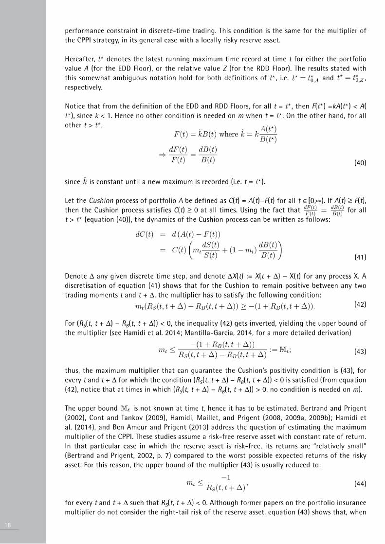
performance constraint in discrete-time trading. This condition is the same for the multiplier of the CPPI strategy, in its general case with a locally risky reserve asset.
Hereafter, denotes the latest running maximum time record at time t for either the portfolio value A (for the EDD Floor), or the relative value Z (for the RDD Floor). The results stated with this somewhat ambiguous notation hold for both definitions of , i.e. and , respectively.
Notice that from the definition of the EDD and RDD Floors, for all t = , then F( ) =kA( ) < A(), since k < 1. Hence no other condition is needed on m when t = . On the other hand, for all
other t > ,
(40)
since is constant until a new maximum is recorded (i.e. t = ).
Let the Cushion process of portfolio A be defined as C(t) = A(t)−F(t) for all t ∈[0,∞). If A(t) ≥ F(t), then the Cushion process satisfies C(t) ≥ 0 at all times. Using the fact that for all t > (equation (40)), the dynamics of the Cushion process can be written as follows:
(41)
Denote Δ any given discrete time step, and denote ΔX(t) := X(t + Δ) − X(t) for any process X. A discretisation of equation (41) shows that for the Cushion to remain positive between any two trading moments t and t + Δ, the multiplier has to satisfy the following condition: (42)
For (RS(t, t + Δ) − RB(t, t + Δ)) < 0, the inequality (42) gets inverted, yielding the upper bound of the multiplier (see Hamidi et al. 2014; Mantilla-García, 2014, for a more detailed derivation)
(43)
thus, the maximum multiplier that can guarantee the Cushion’s positivity condition is (43), for every t and t + Δ for which the condition (RS(t, t + Δ) − RB(t, t + Δ)) < 0 is satisfied (from equation (42), notice that at times in which (RS(t, t + Δ) − RB(t, t + Δ)) > 0, no condition is needed on m).
The upper bound is not known at time t, hence it has to be estimated. Bertrand and Prigent (2002), Cont and Tankov (2009), Hamidi, Maillet, and Prigent (2008, 2009a, 2009b); Hamidi et al. (2014), and Ben Ameur and Prigent (2013) address the question of estimating the maximum multiplier of the CPPI. These studies assume a risk-free reserve asset with constant rate of return. In that particular case in which the reserve asset is risk-free, its returns are “relatively small” (Bertrand and Prigent, 2002, p. 7) compared to the worst possible expected returns of the risky asset. For this reason, the upper bound of the multiplier (43) is usually reduced to:
(44)
for every t and t + Δ such that RS(t, t + Δ) < 0. Although former papers on the portfolio insurance multiplier do not consider the right-tail risk of the reserve asset, equation (43) shows that, when

the reserve asset is locally risky, a sudden and significant increase in its value may also cause a Floor violation. In other words, the right tail of the distribution of the reserve asset returns is of critical importance for the estimation of the upper bound of the multiplier in applications with locally risky reserve assets (as the strategies studied in this paper).
LTS(t, t + Δ) and RTB(t, t + Δ) denote left and right tail estimates of the distributions of RS(t, t + Δ) and RB(t, t + Δ) respectively. Corollary 4 below, together with the assumption that RTB(t, t + Δ) > 0 at all times, shows that a conservative estimate of the upper bound of the multiplier is given by, (45)
that is to say, . In our illustrations we use (time) conditional estimates of the expected shortfall of RS and of −RB to estimate . Notice that since LTS(t, t + Δ) < 0 and RTB(t, t + Δ) > 0, then > 0.
Corollary 4 Consider any pair of assets (S,B) and any two trading instants t and t + Δ, t ∈ [0,∞). The following is a lower bound of the corresponding multiplier upper bound ,
Proof. Recall is defined for t such that (RS(t, t + Δ) − RB(t, t + Δ)) < 0. For notational convenience, hereafter we suppress (t, t + Δ) after RS and RB.Case RB > 0. Suppose
which together with (RS − RB) < 0, implies:
which proves the first condition.
Case RB ≤ 0. Suppose
Notice that if RB ≤ 0 and (RS − RB) < 0 then RS ≤ 0. Thus
which is true from the definition of a return of an asset.
B. Insurable Floor process conditionsWe consider only the non-trivial cases in which F(t0) < A(t0), which holds for all k < 1 for the EDD and RDD Floors and their rolling version. Denote Δ any given discrete time step, and denote ΔX(t) := X(t + Δ) − X(t) for any process X. Then
19

20
In general, for any two times s and t := s + Δ, such that A(s) ≥ F(s),
if (46)
Thus, we have proven by induction that, for all times at which A(t)A(s)≥ F(t)F(s) , no other conditionis needed for A to remain above the Floor value at time t.
Proposition 4 Assume A(t0) > F(t0), and mt ≤ of a type (1) strategy. The Floor process F is insurable if the reserve asset B and F satisfy:
(47)
Proof. From equation (1) we have that
(48)
Recall that for (RS(t, t + 1) − RB(t, t + 1)) < 0, inequality (43) implies m ≤ . Hence, replacing by m in equation (48) implies,
(49)
Assuming the first statement of the first condition in the equation (47), i.e.
(50)
together with inequality (49) implies,
(51)
Hence, as t := s + Δ, condition (50) is a sufficient condition to prove that A(t) ≥ F(t), if (RS(s, s + Δ) − RB(s, s + Δ)) < 0. On the other hand, if (RS(s, s + Δ) − RB(s, s + Δ)) ≥ 0, from equation (48) it is straightforward to see that A(s + Δ)A(s)≥ B(s + Δ) B(s) . This results together with condition (46) above prove that inequality (50) is a sufficient condition to prove that A(t) ≥ F(t) in general. Inequality (50) is the first statement of the Proposition for t = s + Δ, which completes the proof.
C. Proof of Proposition 1Proof. If the value of the portfolio is always above the EDD Floor (16), then
(52)
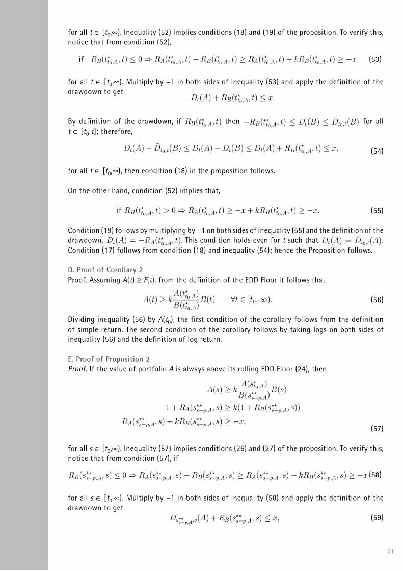
for all t ∈ [t0,∞). Inequality (52) implies conditions (18) and (19) of the proposition. To verify this, notice that from condition (52),
if (53)
for all t ∈ [t0,∞). Multiply by −1 in both sides of inequality (53) and apply the definition of the drawdown to get
By definition of the drawdown, if then for all t ∈ [t0 t]; therefore,
(54)
for all t ∈ [t0,∞), then condition (18) in the proposition follows.
On the other hand, condition (52) implies that,
if (55)
Condition (19) follows by multiplying by −1 on both sides of inequality (55) and the definition of the drawdown, . This condition holds even for t such that .Condition (17) follows from condition (18) and inequality (54); hence the Proposition follows.
D. Proof of Corollary 2Proof. Assuming A(t) ≥ F(t), from the definition of the EDD Floor it follows that
(56)
Dividing inequality (56) by A(t0), the first condition of the corollary follows from the definition of simple return. The second condition of the corollary follows by taking logs on both sides of inequality (56) and the definition of log return.
E. Proof of Proposition 2Proof. If the value of portfolio A is always above its rolling EDD Floor (24), then
(57)
for all s ∈ [t0,∞). Inequality (57) implies conditions (26) and (27) of the proposition. To verify this, notice that from condition (57), if
(58)
for all s ∈ [t0,∞). Multiply by −1 in both sides of inequality (58) and apply the definition of the drawdown to get (59)
21
22
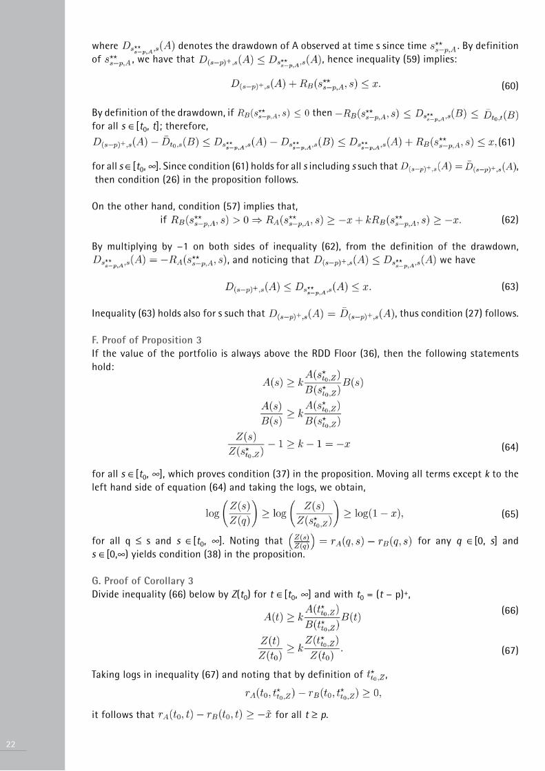
where denotes the drawdown of A observed at time s since time . By definition of , we have that , hence inequality (59) implies:
(60)
By definition of the drawdown, if then for all s ∈[t0, t]; therefore,
(61)
for all s ∈[t0, ∞]. Since condition (61) holds for all s including s such that , then condition (26) in the proposition follows.
On the other hand, condition (57) implies that, if (62)
By multiplying by −1 on both sides of inequality (62), from the definition of the drawdown, , and noticing that we have
(63)
Inequality (63) holds also for s such that , thus condition (27) follows.
F. Proof of Proposition 3If the value of the portfolio is always above the RDD Floor (36), then the following statements hold:
(64)
for all s ∈[t0, ∞], which proves condition (37) in the proposition. Moving all terms except k to the left hand side of equation (64) and taking the logs, we obtain,
(65)
for all q ≤ s and s ∈[t0, ∞]. Noting that for any q ∈[0, s] and s ∈[0,∞) yields condition (38) in the proposition.
G. Proof of Corollary 3Divide inequality (66) below by Z(t0) for t ∈[t0, ∞] and with t0 = (t − p)+, (66)
(67)
Taking logs in inequality (67) and noting that by definition of ,
it follows that for all t ≥ p.

H. Proving the Insurability of EDD and RDD FloorsIn what follows, we show that both the RDD and EDD Floors are insurable. Unless indicated, in this section, denotes the latest running maximum time record at time t for either the portfolio value A (for the EDD Floor) or the relative value Z (for the RDD Floor). The results stated with this somewhat ambiguous notation hold for both definitions of , i.e., and , respectively.
As aforementioned, the EDD and RDD Floors can be defined for a rolling look-back period p by setting t0 = (t − p)+. Proposition 5 below holds for all the cases considered in the proof for the rolling period Floors by replacing t0 = (t − p)+. However, for any s < t, the proof below does not include the case s < < s < t because by definition of , for t0 = 0 or any other constant value of t0 < s (for the no rolling period Floors), that case is not possible. To see this, notice that by definition of , if t0 = 0, then and .
Proposition 5 Let (68)
be the Floor process of a type (1) strategy A. If mt ≤ , then F(t) ≤ A(t) for all t.
Proof. Consider any two times, t1 < t2.• Denote Case 0 all cases such that t2 = (i.e., for all ≤ t1). In such cases, for k < 1.
Hereafter we show that, for all remaining possibilities with < t2 we have:14
• Case 1 t1 = = < t2, then F(t1) ≤ A(t1) and F(t2) ≤ A(t2).
• Case 2 = < t1 < t2, then F(t1) ≤ A(t1) and F(t2) ≤ A(t2).
• Case 3 ≤ t1 < < t2, then F(t1) ≤ A(t1) and F(t2) ≤ A(t2).
Notice that for Case 1 and Case 2, = . Thus, replacing A( ) and B( ) with = in the Floor formula yields,
hence from Proposition 4, it follows that F(t2) ≤ A(t2) in Case 1 and Case 2.
Notice as well that in Case 1 by definition of the Floor it also follows that F(t1) ≤ A(t1), since in that case t1 = . Furthermore, notice that Case 2 = < t1 < t2 can be split in two cases by time pairs. First, = < t1 corresponds to Case 1 setting t1 as t2, which means that, in Case 2, we also have F(t1) ≤ A(t1).
In a similar way, Case 3 ≤ t1 < < t2 can be split in three cases, by time pairs. First, ≤ t1, contains the trivial case t1 = (for which F( ) < A( ) follows by definition of F) and < t1, which corresponds to Case 1 setting t1 as t2.
Second, t1 < corresponds to Case 0. Third, < t2 corresponds to Case 1. Hence, for Case 3, F(t2) ≤ A(t2) and F(t1) ≤ A(t1).
Finally, notice that at inception date t0 = t1 = , hence F(t0) < A(t0). Furthermore, for t2 = t0 + δ, for an arbitrarily small δ, then either t2 = , which corresponds to a particular Case 0 in which F(t1) ≤ A(t1), or t0 = t1 = = < t2, which corresponds to Case 1.
2314 - Notice that, in absence of a rolling period, the case < < t1 < t2, is not feasible.

24
This means that Case 0 is always preceded by a case in which F(t1) ≤ A(t1) and F(t2) ≤ A(t2). Thus, for any t1 and t2, F(t1) ≤ A(t1) and F(t2) ≤ A(t2).
Hereafter, we consider the case in which and ,which is only relevant for the rolling period definitions of EDD and RDD Floors, respectively.
H.1 Insurability check for rolling RDD FloorFor any two times s and t such that s < < s < t we have,
(69)
According to Proposition 4, if , then the reserve asset should super-replicate the Floor index, i.e. .
For the opposite condition to hold,
then the following must hold:
Thus Proposition (4) cannot be violated in any case in which , which is the only case not covered on the proof of the global EDD and RDD floors above. This proves that the rolling RDD Floor is insurable.
H.2 Insurability check for rolling EDD FloorHereafter we first show that the naive version of the rolling EDD Floor is not insurable in general and provide the conditions under which the Floor can be violated even if the multiplier is below its upper bound. The definition of the insurable rolling EDD Floor version follows directly from those conditions.
The proof above on the insurability if the EDD and RDD Floors does not include the case s < < s< t because by definition of with t0 = 0 for the no rolling period Floors, that case is not possible. On the other hand, for the naive rolling EDD Floor, p < ∞, such case is possible as the rolling running maximum can (eventually) decrease over time, i.e. (70)
In such case, we now show that if contemporaneously , the Floor can be violated (i.e. it is not insurable), and a modified definition of the Floor in which such condition cannot hold is provided.
From the definition of the rolling EDD Floor, if at time t, A(t) < F(t), then
(71)

On the other hand, if mt ≤ Mt, from equation (49), for t = s + Δ
(72) (73)
Replacing A(t), in the particular case for which (73) is an equality in equation (71) yields,
(74)
Hence, the naive EDD Floor with a rolling horizon is not insurable in the particular case in which the two conditions (70) and (74) hold at the same time.
Define the set
(75)
which contains all times at which condition (74) is satisfied. Using the notation of the rolling running maximum, i.e. , condition (70) can be restated as (76)
Hence, the naive version of the rolling EDD Floor is not insurable when conditions (75) and (76) hold at the same time. We now define a conditional version of the rolling EDD Floor in which the oldest date considered to determine the rolling running maximum does not always move forward in time continuously, i.e. t0 = t − p for all t > p, but only at times at which conditions (75) and (76) are not satisfied. This implies a conditional version of , which is equal to its unconditional rolling version except at times when (75) and (76) hold. For this conditional version, before resetting the oldest date t0 that determines the rolling running maximum, to t0+Δt, we check whether the two conditions are satisfied; if the conditions hold, then t0 is not updated. Formally, let the conditional rolling maximum time process be defined as
(77)
The definition of the rolling EDD is similar to its naive version, with the exception that its reference time for the running maximum of A only rolls forward if conditions (75) and (76) are satisfied, and is equal to its preceding reference time otherwise. This modified or conditional version of the rolling EDD Floor is insurable by construction.
Hereafter we present an algorithm with a function that illustrates the definitions of the (conditional) rolling EDD Floor and .
25

26
Tables
Table 1: Distributions summaries of regression coefficient βmkt and R2 of EW S&P 500 index regressed on the CW S&P 500 index, and of conditional multiplier upper bound estimate of EDD overlay strategies.
Table 2: Performance of EDD(p,k × 100) hedging overlay strategies. The underlying asset is the S&P 500 equal weighted index (EW 500).

Table 3: Performance of the benchmark (B) cap-weighted S&P 500 index (CW 500), the performance asset (S) equal-weighted S&P 500 index (EW 500), the CPPI(k × 100) and the RDD(p years,k × 100) strategies.
FiguresFig. 1 - Leverage ratio (left panel) and hedging overlay weight (right panel) distributions of EDD strategies with k = {0.75, 0.8, 0.85} and rolling horizon i.e. p = {0.5, 1,∞} years. The out-of-sample period of the Backtest is 05/1977 to 12/2010.
27

28
Fig. 2 - Distributions of RDD strategy weights (left panel) and multipliers (right panel), for k = {0.75, 0.8, 0.85} and rolling horizon i.e. p = {3, 5,∞} years. The out-ofsample period of the Backtest is 05/1977 to 12/2010.
References• Alster, N. The cash cushion, making a comeback in mutual funds. Retrieved from http: //www.nytimes.com. The New York Times, October 5 2013.
• Amenc, N., P. Malaise, and L. Martellini (2004). Revisiting core-satellite investing: a dynamic model of relative risk management. Journal of Portfolio Management 31 (1), 64–75.
• Ang, A., S. Gorovyy, and G. B. Van Inwegen (2011). Hedge fund leverage. Journal of Financial Economics 102 (1), 102–126.
• Basak, S., A. Shapiro, and L. Teplá (2006). Risk management with benchmarking. Management Science 52 (4), 542–557.
• Ben Ameur, H. and J. Prigent (2013). Portfolio insurance: Gap risk under conditional multiples. INSEEC, Paris working paper.
• Bertrand, P. and J.-L. Prigent (2002). Portfolio insurance: the extreme value approach to the CPPI method. Finance 23 (2), 69–86.
• Black, F. and R. Jones (1987). Simplifying portfolio insurance. The Journal of Portfolio Management 14 (1), 48–51.
• Black, F. and A. Perold (1992). Theory of constant proportion portfolio insurance. Journal of Economic Dynamics and Control 16 (3-4), 403–426.
• Blackrock. Do you realise the cost of holding cash? Retrieved from https://www2. blackrock.com. Blackrock website, chart of the week June 17 2013.
• Browne, S. (1999). Beating a moving target: Optimal portfolio strategies for outperforming a stochastic benchmark. Finance and Stochastics 3 (3), 275–294.
• Browne, S. (2000). Risk-constrained dynamic active portfolio management. Management Science 46 (9), 1188–1199.
• Carr, P., H. Zhang, and O. Hadjiliadis (2011). Maximum drawdown insurance. International Journal of Theoretical and Applied Finance 14 (08), 1195–1230.
• Chekhlov, A., S. Uryasev, and M. Zabarankin (2000). Portfolio optimisation with drawdown constraints. Department of Industrial & Systems Engineering, University of Florida.
• Chekhlov, A., S. Uryasev, and M. Zabarankin (2005). Drawdown measure in portfolio optimisation. International Journal of Theoretical and Applied Finance 8 (01), 13–58.

• Cont, R. and P. Tankov (2009). Constant proportion portfolio insurance in the presence of jumps in asset prices. Mathematical Finance 19 (3), 379–401.
• Cvitanic, J. and I. Karatzas (1995). On portfolio optimisation under “drawdown” constraints. IMA volumes in mathematics and its applications 65, 35–35.
• DeMiguel, V., L. Garlappi, and R. Uppal (2009). Optimal versus naive diversification: How inefficient is the 1/N portfolio strategy? Review of Financial Studies 22 (5), 1915–1953.
• Douady, R., A. Shiryaev, and M. Yor (2000). On probability characteristics of “downfalls” in a standard Brownian motion. Theory of Probability & Its Applications 44 (1), 29–38.
• Drechsler, I. (2014). Risk choice under high-water marks. Review of Financial Studies, hht081.
• Elie, R. and N. Touzi (2008). Optimal lifetime consumption and investment under a drawdown constraint. Finance and Stochastics 12 (3), 299–330.
• Engle, R. (2001). Garch 101: The use of ARCH/GARCH models in applied econometrics. Journal of economic perspectives, 157–168.
• Estep, T. and M. Kritzman (1988). TIPP: Insurance without complexity. The Journal of Portfolio Management 14 (4), 38–42.
• Fernholz, E. (2002). Stochastic portfolio theory. Springer Verlag.
• Goetzmann, W. N., J. E. Ingersoll, and S. A. Ross (2003). High-water marks and hedge fund management contracts. The Journal of Finance 58 (4), 1685–1718.
• Grossman, S. and J. Vila (1992). Optimal dynamic trading with leverage constraints. Journal of Financial and Quantitative Analysis 27 (02), 151–168.
• Grossman, S. J. and Z. Zhou (1993). Optimal investment strategies for controlling drawdowns. Mathematical Finance 3 (3), 241–276.
• Guasoni, P. and J. Obloj (2011). The incentives of hedge fund fees and high-water marks.
• Hadjiliadis, O. and J. Vecer (2006). Drawdowns preceding rallies in the brownian motion model. Quantitative Finance 6 (5), 403–409.
• Hamidi, B., B. Maillet, and J.-L. Prigent (2008). A Time-varying Proportion Portfolio Insurance Strategy based on a CAViaR Approach. Working paper, University of Cergy-THEMA.
• Hamidi, B., B. Maillet, and J.-L. Prigent (2009a). A caviar modelling for a simple timevarying proportion portfolio insurance strategy. Bankers, Markets & Investors 102, 4–21.
• Hamidi, B., B. Maillet, and J.-L. Prigent (2009b). Financial Risks, Chapter A Risk Management Approach for Portfolio Insurance Strategies, pp. 117–132. Economica.
• Hamidi, B., B. Maillet, and J.-L. Prigent (2012). Time-varying proportion portfolio insurance with autoregressive conditional gap risk duration. Technical report, Working paper, University of Paris I and Cergy-THEMA.
• Hamidi, B., B. Maillet, and J.-L. Prigent (2014). A dynamic autoregressive expectile for time-invariant portfolio protection strategies. Journal of Economic Dynamics and Control.
• Healy, A. D. and A. W. Lo (2009). Jumping the gates: Using beta-overlay strategies to hedge liquidity constraints. Journal of Investment Management (3), 11.
• Kim, D. (2011). Revelance of maximum drawdown in the investment fund selection problem when utility is nonadditive. Journal of Economic Research 16 (3), 257–289.
• Labuszewski, J. W. and B. Vietmeier (2005). CME e-mini stock index futures vs. exchange traded funds. CME Research & Product Developement.
• Lan, Y., N. Wang, and J. Yang (2013). The economics of hedge funds. Journal of Financial Economics. 29
30
• Magdon-Ismail, M., A. Atiya, A. Pratap, and Y. Abu-Mostafa (2004). On the maximum drawdown of a Brownian motion. Journal of Applied Probability 41 (1), 147–161.
• Mantilla-García, D. (2014). Growth optimal portfolio insurance for long-term investors. Journal Of Investment Management (forthcoming).
• Martellini, L. and V. Milhau (2009). Measuring the benefits of dynamic asset allocation strategies in the presence of liability constraints. Technical report, Working paper EDHEC-Risk.
• McNeil, A. J. and R. Frey (2000). Estimation of tail-related risk measures for heteroscedastic financial time series: An extreme value approach. Journal of Empirical Finance 7 (3), 271–300.
• Pangeas, S. and M. M. Westerfield (2009). High watermarks: High risk appetites? hedge fund compensation and portfolio choice. The Journal of Finance.
• Patton, A. J. and T. Ramadorai (2013). On the high-frequency dynamics of hedge fund risk exposures. The Journal of Finance 68 (2), 597–635.
• Perold, A. (1986). Constant proportion portfolio insurance. Technical report, Harvard Business School.
• Pospisil, L. and J. Vecer (2008). PDE methods for the maximum drawdown. Journal of Computational Finance 12 (2), 59–76.
• Pospisil, L. and J. Vecer (2010). Portfolio sensitivity to changes in the maximum and the maximum drawdown. Quantitative Finance 10 (6), 617–627.
• Pospisil, L., J. Vecer, and O. Hadjiliadis (2009). Formulas for stopped diffusion processes with stopping times based on drawdowns and drawups. Stochastic Processes and Their Applications 119 (8), 2563–2578.
• Roche, H. (2013). Optimal consumption and investment strategies under wealth ratcheting. In 30th International French Finance Association Conference 2013, EM Lyon.
• Yang, Z. and L. Zhong (2012). Optimal portfolio strategy to control maximum drawdown—the case of risk based dynamic asset allocation. Available at SSRN 2053854 .
• Zhang, H. (2014). Occupation times, drawdowns, and drawups for one-dimensional regular diffusions. Advances in Applied Probability (forthcoming).
• Zhang, H. and O. Hadjiliadis (2010). Drawdowns and rallies in a finite time-horizon. Methodology and Computing in Applied Probability 12 (2), 293–308.
• Zhang, H. and O. Hadjiliadis (2012). Drawdowns and the speed of market crash. Methodology and Computing in Applied Probability 14 (3), 739–752.
• Zhang, H., T. Leung, and O. Hadjiliadis (2013). Stochastic modelling and fair valuation of drawdown insurance. Insurance: Mathematics and Economics.

Founded in 1906, EDHEC Business School offers management education at undergraduate, graduate, post-graduate and executive levels. Holding the AACSB, AMBA and EQUIS accreditations and regularly ranked among Europe’s leading institutions, EDHEC Business School delivers degree courses to over 6,000 students from the world over and trains 5,500 professionals yearly through executive courses and research events. The School’s ‘Research for Business’ policy focuses on issues that correspond to genuine industry and community expectations.
Established in 2001, EDHEC-Risk Institute has become the premier academic centre for industry-relevant financial research. In partnership with large financial institutions, its team of ninety permanent professors, engineers, and support staff, and forty-eight research associates and affiliate professors, implements six research programmes and sixteen research chairs and strategic research projects focusing on asset allocation and
risk management. EDHEC-Risk Institute also has highly significant executive education activities for professionals. It has an original PhD in Finance programme which has an executive track for high level professionals. Complementing the core faculty, this unique PhD in Finance programme has highly prestigious affiliate faculty from universities such as Princeton, Wharton, Oxford, Chicago and CalTech.
In 2012, EDHEC-Risk Institute signed two strategic partnership agreements with the Operations Research and Financial Engineering department of Princeton University to set up a joint research programme in the area of risk and investment management, and with Yale School of Management to set up joint certified executive training courses in North America and Europe in the area of investment management.
Copyright © 2014 EDHEC-Risk Institute
EDHEC-Risk Institute393 promenade des AnglaisBP 3116 - 06202 Nice Cedex 3FranceTel: +33 (0)4 93 18 78 24
EDHEC Risk Institute—Europe 10 Fleet Place, LudgateLondon EC4M 7RBUnited KingdomTel: +44 207 871 6740
EDHEC Risk Institute—Asia1 George Street#07-02Singapore 049145Tel: +65 6438 0030
www.edhec-risk.com
For more information, please contact: Carolyn Essid on +33 493 187 824 or by e-mail to: [email protected]
EDHEC Risk Institute—North AmericaOne Boston Place, 201 Washington StreetSuite 2608/2640 — Boston, MA 02108United States of AmericaTel: +1 857 239 8891
EDHEC Risk Institute—France 16-18 rue du 4 septembre75002 Paris FranceTel: +33 (0)1 53 32 76 30