How efficiently do 3-manifolds bound 4-manifolds?

Dylan ThurstonJoint work with Francesco Costantino

Knots in Vancouver

July 23, 2004

−→

Part 1: Context

2

Representing 3-manifolds

Triangulations:

• Natural representation.

• Easy to construct from other representations.

• Compute some invariants (Turaev-Viro).

• Difficult to visualise.

Surgery diagrams:

• Compute invariants (Casson, Witten-Reshetikhin-Turaev).

• In practice, gives simple representations of small manifolds.

• How much do you lose in principle?

• Nearly the same as giving a 4-manifold bounded by the 3-manifold.

3

Problem statement

Definition. The complexity of an (oriented) d-manifold is the minimal num-ber of simplices in a triangulation.

C(Md) = minTriang. ∆ of M

# of d-simplices in ∆

The 3-dimensional isoperimetric function gives the minimal complexity of4-manifolds bounding 3-manifolds of a given complexity.

G3(n) = maxM3|C(M)≤n

minN4|∂N∼=M

C(N)

Question. What is the asymptotic growth rate of G3(n)?

Theorem (Costantino-T.). There is a constant k > 0 so that

G3(n) ≤ kn2

Remark. A related question would require that the triangulation of the 4-manifold on the boundary agree with a given triangulated 3-manifold. Wealso get a quadratic bound in this case.

4

Previous work

Constructive proofs that 3-manifolds bound 4-manifolds give estimates forG3(n).

Proofs we’re aware of:

• Rohlin (1951): Based on a generic map f : M 3 → R5. Probably gives

G3(n) ≤ kn4.

• Thom (1954): Homotopy-theoretic. Hard to get explicit bounds onG3(n).

• Lickorish (1962), Rourke (1985), Matveev-Polyak (1994): Inductiveproofs, based on mapping class group. Use the inductive hypothesistwice, so get exponential bounds for G3(n) at best.

• Costantino-T.: Based on a generic map f : M 3 → R2. Gives G3(n) ≤

kn2.

5

Analogous problems

We could also consider:

Question. What is the isoperimetric function Gsurf for polygonal curvesbounding triangulated surfaces in R

3?

Theorem (Hass-Lagarias). 12n2 ≤ Gsurf(n) ≤ 7n2.

Question. What is the isoperimetric function Gdisk for unknotted polygonalcurves bounding triangulated disks in R

3?

Theorem (Hass-Lagarias-Snoeyink-W. Thurston). c1An ≤ Gdisk(n) ≤ c2B

n2

.

Question. What is the bound GPachner of the number of Pachner movesrequired to turn a triangulation with n tetrahedra into a standard one?

Theorem (King, Mijatovic). GPachner(n) ≤ c1An

2

.

Note that a sequence of Pachner moves gives a triangulation of the 4-ball.On the other hand, coning to a point gives a triangulation with many fewer4-simplices. Perhaps bounding the geometry of the triangulation of the 4-ballin some way gives an appropriate analogous question to the growth of Gdisk.

6

Part 2: The proof

7

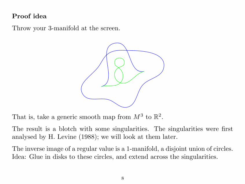
Proof idea

Throw your 3-manifold at the screen.

That is, take a generic smooth map from M 3 to R2.

The result is a blotch with some singularities. The singularities were firstanalysed by H. Levine (1988); we will look at them later.

The inverse image of a regular value is a 1-manifold, a disjoint union of circles.Idea: Glue in disks to these circles, and extend across the singularities.

8

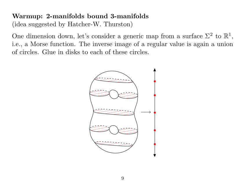
Warmup: 2-manifolds bound 3-manifolds

(idea suggested by Hatcher-W. Thurston)

One dimension down, let’s consider a generic map from a surface Σ2 to R1,

i.e., a Morse function. The inverse image of a regular value is again a unionof circles. Glue in disks to each of these circles.

−→

9

Singularites of maps from surfaces to R

A critical point is either a saddle point or a maximum/minimum locally inthe domain.

The inverse image of each regular point is an oriented 1-manifold, so theorientations into a saddle point must alternate:

−→ and

Therefore the inverse image of a saddle value is a figure 8, and the inverseimage of its neighborhood is a pair of pants.

10

Filling in the 3-manifold

We can now finish constructing the 3-manifold. Take the surface cross aninterval and glue in a 2-handle to the each circle in the inverse image of aregular point.

By the analysis above, the boundary remaining near each critical value is asphere, in one of two ways. Glue in a ball to each one.

−→

11

The Stein factorization

Let’s view this construction from a more global point of view. For any mapf from a compact manifold, we can consider the Stein factorization f = g ◦h

where the fibers of g are connected and h is finite-to-one.

−→ −→

At generic points, the surface Σ is a circle bundle over the Stein graph andthe 3-manifold is a disk bundle. Alternatively, the 3-manifold collapses ontothe Stein graph.

12

3-manifolds

In the case of 3-manifolds mapping to R2, in codimension 1 the singularities

look like the previous singularities (surface to R), crossed with an interval.

In codimension 2 locally in the domain, the only new singularity is a kind ofcusp. It can be viewed as two critical points of index 0 and 1 meeting andcancelling.

However, this singularity turns out to play little role. More interesting is thecrossing of two codimension 1 saddle-type singularities.

13

Crossing singularities

There are two singular points in the inverse image of a crossing of two saddletype singularities. Following the orientations as before, there are two waysto connect up these two singularities to get a connected fiber.

(a) (b)

We will assume that our generic map has no singularities of type (b), since:

• Type (b) is similar to type (a), only slightly more complicated;

• A singularity of type (b) can be perturbed a little to get two singu-larities of type (a).

14

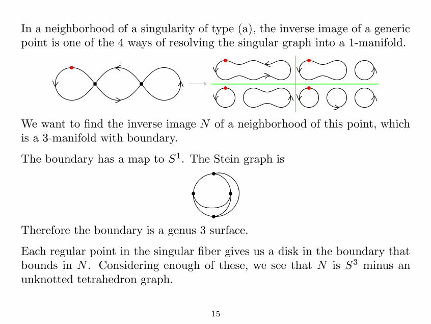
In a neighborhood of a singularity of type (a), the inverse image of a genericpoint is one of the 4 ways of resolving the singular graph into a 1-manifold.

−→

We want to find the inverse image N of a neighborhood of this point, whichis a 3-manifold with boundary.

The boundary has a map to S1. The Stein graph is

Therefore the boundary is a genus 3 surface.

Each regular point in the singular fiber gives us a disk in the boundary thatbounds in N . Considering enough of these, we see that N is S3 minus anunknotted tetrahedron graph.

15

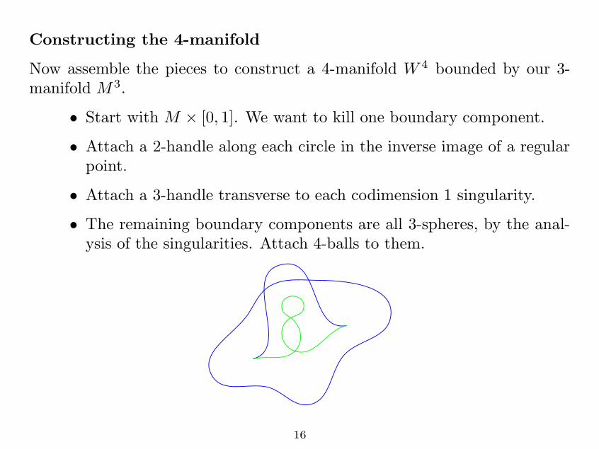
Constructing the 4-manifold

Now assemble the pieces to construct a 4-manifold W 4 bounded by our 3-manifold M3.

• Start with M × [0, 1]. We want to kill one boundary component.

• Attach a 2-handle along each circle in the inverse image of a regularpoint.

• Attach a 3-handle transverse to each codimension 1 singularity.

• The remaining boundary components are all 3-spheres, by the anal-ysis of the singularities. Attach 4-balls to them.

16

A more global view

As in the case of surfaces mapping to R, we can consider the Stein factoriza-tion of our map from M 3 to R

2.

The resulting Stein surface is a 2-complex. It has a number of local models,including

• the plane R2 at regular points;

• a 3-page book from codimension 1 singularities; and

• the cone over the graph we found around the crossing of singularities.

among a few others.

The 4-manifold collapses onto the Stein surface. As before, the 4-manifold isgenerically a disk bundle over the surface and the 3-manifold is generically acircle bundle.

We will say more on these surfaces later.

17

Starting from a triangulation

So far, we have been working with generic smooth maps. This has two prob-lems:

• It involves analysis to find the generic singularities;

• To bound the complexity, we want to start from a triangulation.

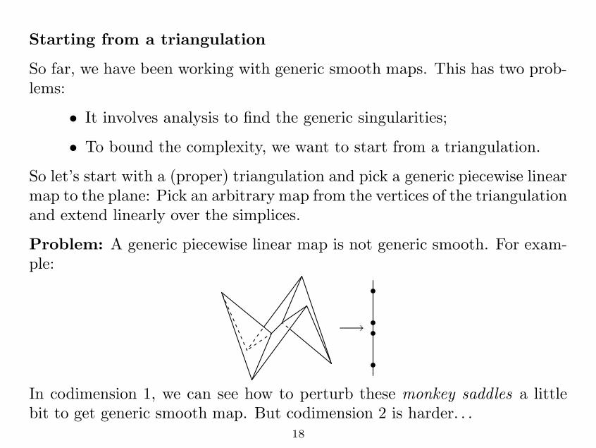
So let’s start with a (proper) triangulation and pick a generic piecewise linearmap to the plane: Pick an arbitrary map from the vertices of the triangulationand extend linearly over the simplices.

Problem: A generic piecewise linear map is not generic smooth. For exam-ple:

−→

In codimension 1, we can see how to perturb these monkey saddles a littlebit to get generic smooth map. But codimension 2 is harder. . .

18

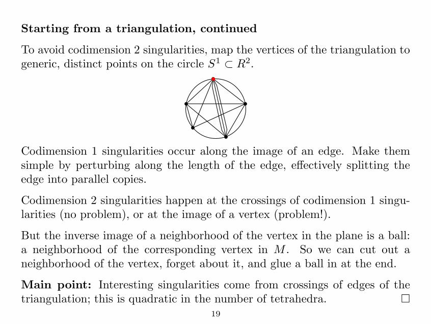
Starting from a triangulation, continued

To avoid codimension 2 singularities, map the vertices of the triangulation togeneric, distinct points on the circle S1 ⊂ R2.

Codimension 1 singularities occur along the image of an edge. Make themsimple by perturbing along the length of the edge, effectively splitting theedge into parallel copies.

Codimension 2 singularities happen at the crossings of codimension 1 singu-larities (no problem), or at the image of a vertex (problem!).

But the inverse image of a neighborhood of the vertex in the plane is a ball:a neighborhood of the corresponding vertex in M . So we can cut out aneighborhood of the vertex, forget about it, and glue a ball in at the end.

Main point: Interesting singularities come from crossings of edges of thetriangulation; this is quadratic in the number of tetrahedra. �

19

Part 3: Going further

20

4-manifolds bounding 5-manifolds?

Why doesn’t this proof work to show that 4-manifolds bound 5-manifolds?Start the same way: pick a generic map from your 4-manifold to R

3. . .

There are some new codimension 3 singularities. For some of them, theinverse image of a neighborhood, filled in around the boundary, is not S4,

but rather CP2 or CP

2.

This does give a proof that every smooth 4-manifold is cobordant to a union

of CP2 and CP

2’s.

If you want to get bounds on the complexity, you also need to worry aboutgeneric PL maps which are not generic smooth maps in codimension 2.

21

The shadow world

A soap bubble locally looks like:

• A plane;

• A 3-page book; or

• A cone over the 1-skeleton of a tetrahedron.

A 2-complex Σ whose only singularities are in the list above is called a simplepolyhedron.

If such a Σ is embedded in a 4-manifold W in a locally flat way, and W col-lapses onto Σ, then we call Σ a shadow representation of W and its bound-ary ∂W .

Contrast this with the standard spines for 3-manifolds, where the 3-manifoldis generically an interval bundle over Σ, rather than a disk bundle.

To determine W from Σ, also need to specify some integers or half-integers(the gleams) on the 2-dimensional faces. If Σ is a closed surface, the gleamis the Euler class of the disk bundle. In general, it is a relative Euler class.

22

Shadow number and Gromov norm

Definition. The shadow number of a 3-manifold is the minimum number ofvertices in a shadow representation of the manifold.

There is an improved version of the main theorem that deals with ideal tri-angulation or spun ideal triangulations:

Theorem. A manifold with a (spun) ideal triangulation with n tetrahedrahas a shadow diagram with O(n2) vertices.

Theorem. The 3-manifolds with shadow diagrams with no vertices are ex-actly the graph manifolds (manifolds which can be cut up into Seifert-fiberedpieces).

Theorem (W. Thurston). A hyperbolic manifold with volume V has a spunideal triangulation with O(V ) tetrahedra.

Corollary. A manifold M with Gromov norm ‖M‖ satisfying the Geometriza-tion Conjecture has a shadow diagram has shadow number S satisfying

C1‖M‖ ≤ S ≤ C2‖M‖2

for suitable constants C1, C2.

23

Open questions

• Lower bounds or better upper bounds for G3, 3-manifolds bounding4-manifolds.

• Lower bounds for GPachner, Pachner moves to make a triangulationof S3 standard.

• Bounds for 3-manifolds to bound special 4-manifolds, like simply-connected or spin.

• Lower bounds with a coarser notion of the complexity of the 4-manifold (e.g., the order of the second homology).

One approach to a lower bound for G3:

• Pick an invariant I of 3-manifolds that is defined from a 4-manifoldbounded by the 3-manifold;

• Show that I is linearly bounded by the complexity of the 4-manifold;

• Find a family of 3-manifolds for which I grows quadratically in thecomplexity of the 3-manifold.

24