durham e-theses tool life prediction and management for an
TRANSCRIPT

Durham E-Theses
Tool life prediction and management for an integrated
tool selection system
Alamin, Bubakar B.
How to cite:
Alamin, Bubakar B. (1996) Tool life prediction and management for an integrated tool selection system,Durham theses, Durham University. Available at Durham E-Theses Online: http://etheses.dur.ac.uk/5287/
Use policy
The full-text may be used and/or reproduced, and given to third parties in any format or medium, without prior permission orcharge, for personal research or study, educational, or not-for-pro�t purposes provided that:
• a full bibliographic reference is made to the original source
• a link is made to the metadata record in Durham E-Theses
• the full-text is not changed in any way
The full-text must not be sold in any format or medium without the formal permission of the copyright holders.
Please consult the full Durham E-Theses policy for further details.
Academic Support O�ce, Durham University, University O�ce, Old Elvet, Durham DH1 3HPe-mail: [email protected] Tel: +44 0191 334 6107
http://etheses.dur.ac.uk

To my family

TOOL L I F E PREDICTION AND MANAGEMENT FOR
AN INTEGRATED TOOL SELECTION SYSTEM The copyright of this thesis rests with the author. No quotation from it should be published without the written consent of the author and information derived from it should be acknowledged.
A thesis submitted to the
School of Engineering
University of Durham
for the degree of
Doctor of Philosophy
by
Bubakar B. Alamin
April 1996
-8 OCT 1997

ABSTRACT
In machining, it is often difficult to select appropriate tools (tool holder and insert),
machining parameters (cutting speed, feed rate and depth of cut) and tool replacement
times for all tools due to the wide variety of tooling options and the complexity of the
machining operations. Of particular interest is the complex interrelationships between
tool selection, cutting data calculation and tool life prediction and control.
Numerous techniques and methods of measuring and modelling tool wear, particularly
in turning operations were reviewed. The characteristics of these methods were
analysed and it was found that most tool wear studies were self-contained without any
obvious interface with tool selection. The work presented herein deals with the
development of an integrated, off-line tool life control system (TLC). The tool life
control system (TLC) predicts tool life for the various mming operations and for a wide
variety of workpiece materials. TLC is a closed-loop system combining algorithms with
feedback based on direct measurement of flank wear. TLC has been developed using
Crystal, which is a rule-based shell and statistical techniques such as multiple regression
and the least-squares method. TLC consists of five modules namely, the technical
planning of the cutting operation (TPO), tool life prediction (TLP), tool life assessor
(TLA), tool life management (TLM) and the tool wear balancing and requirement
planning (TRP).
The technical planning of the cutting operation (TPO) module contains a procedure to
select tools and generate efficient machining parameters (cutting velocity, feed rate and
depth of cut) for turning and boring operations. For any selected insert grade, material
sub-class, type of cut (finishing, medium-roughing and roughing) and type of cutting
fluid, the tool life prediction (TLP) module calculates the theoretical tool life value
(Tsugg) based on tool life coefficients derived from tool manufacturers' data. For the
selected operation, the tool life assessor (TLA) generates a dynamic multiple regression
to calculate the approved tool life constants (InC, 1/a, 1/p) based on the real tool life
data collected from experiments. These approved constants are used to calculate a

modified tool life value (Tmod) for the given operation. The stochastic nature of tool life
is taken into account, as well as the uncertainty of the available information by
introducing a 95% confidence level for tool life.
The tool life management module (TLM) studies the variations in tool life data
predicted by TLP and TLA and the approved tool life data collected from the shop floor
and provides feedback concerning the accuracy of tool life predictions. Finally, the tool
life balancing and requirement planning (TRP) methods address the problem of
controlling and balancing the wear rate of the cutting edge by the appropriate alteration
of cutting conditions so that each one wil l machine the number of parts that optimize the
overall tool changing strategy. Two new tool changing strategies were developed based
on minimum production cost, with very encouraging results.
Cutting experiments proved that the state of wear and the tool life can be predicted
efficiently by the proposed model. The resulting software can be used by machine
manufacturers, tool consultants or process planners to achieve the integrated planning
and control of tool life as part of the tool selection and cutting data calculation activity.

ACKNOWLEDGEMENTS
I would like to acknowledge the support and assistance of Dr P. G. Maropoulos
throughout this research. Paul's enthusiasm and knowledge of the subject area has been
a source of inspiration and motivation. His friendly manner, encouragement and general
assistance made the production of this thesis markedly more manageable.
I would like to acknowledge all the technical staff of the School of Engineering,
especially Alan Swann for the unforgettable camaraderie we shared in the workshop -
his tolerance and support are strongly appreciated.
I want to thank may wife and my family for their constant patience and support
throughout the period of my study.
Thanks are also due to all my friends in Libya for their warm feelings and supporting
messages.
Finally, I am deeply grateful to the Libyan Govemment and in particular the Ministry of
Education, who made my studies possible in providing the opportunity and support for
this work to be carried out.
Il l

CONTENTS
ABSTRACT
ACKNOWLEDGEMENTS
CONTENTS
LIST OF FIGURES
LIST OF TABLES
CHAPTER 1 INTRODUCTION 1
1.1 TOOL SELECTION WITHIN PROCESS PLANNING 1
1.2 TOOL L I F E CONTROL AND MANAGEMENT WITHIN TOOL SELECTION 4
1.3 TOOL WEAR AND TOOL LIFE: DEFINITION AND THEORY 5
1.3.1 Mechanisms of wear 7
1.3.2 Types of wear 9
1.3.3 Progressive tool wear 12
1.3.4 Parameters influencing tool wear and tool life for turning 14
1.4 WEAR MEASUREMENT TECHNIQUES 16
1.4.1 Direct methods for measuring tool wear 18
1.4.1.1 Optical measurement 18
1.4.1.2 Workpiece size changing 19
1.4.1.3 Distance from tool post to workpiece 20
1.4.1.4 Tool/work junction electrical resistance measurement 22
1.4.1.5 Radioactive techniques 22
1.4.1.6 Analysis of wear particles on the chips 22
1.4.2 Indirect methods for measuring tool wear 23
1.4.2.1 Cutting forces measurement ' 24
1.4.2.2 Acoustic emission (AE) 26
1.4.2.3 Sound 29
1.4.2.4 Vibration 30
1.4.2.5 Variation of power input 31
1.4.2.6 Cutting temperature measurement 31
1.4.2.7 Surface roughness measurement 33
1.5 ANALYTICAL MODELS FOR TOOL L I F E PREDICTION 33
1.6 AIMS AND OBJECTIVES OF PRESENT WORK 42
CHAPTER 2 OVERALL STRUCTURE OF TOOL LIFE CONTROL CTLC) 44
2.1 SYSTEM'S DATABASE REQUIREMENTS 49
2.2 DATABASE MANAGEMENT FUNCTIONS 54
IV
2.2.1 Search for a record 54
2.2.2 Edit a record 55
CHAPTER 3 TECHNICAL PLANNING OF THE CUTTING OPERATION 56
3.1 SPECinCATION AND FUNCTIONALITY OF I P G 56
3.1.1 Operation definition 57
3.1.2 Tool holder selection 58
3.1.3 Material selection 59
3.1.4 Insert selection 59
3.1.5 Depth of cut and feed rate calculations 62
3.1.5.1 Finishing operation 62
3.1.5.2 Roughing operation 63
3.1.6 Cutting forces 65
3.1.7 Force constraints 67
3.1.8 Cutting velocity 71
CHAPTER 4 TOOL L I F E PREDICTION (TLP) 74
4.1 AUTOMATIC R U L E INDUCTION SYSTEM 76
4.2 CALCULATIONS OF THE THEORETICAL TOOL L I F E CONSTANTS 79
4.2.1 Multiple regression 81
4.3 TOOL L I F E CALCULATION C R I T E R L \ 83
4.3.1 Tool life for user defined cutting conditions 83
4.3.2 Tool life for minimum production cost 84
4.3.3 Tool life for minimum production time 87
CHAPTER 5 INITIAL TOOL L I F E TESTS 89
5.1 APPARATUS USED 90
5.1.1 The centre ladie 90
5.1.2 Tool holder and inserts 91
5.1.3 Workpiece material 92
5.1.4 Measuring microscope 92
5.2 TOOL FAILURE C R I T E R L \ 93
5.3 THEORETICAL CALCULATIONS AND RESULTS 95
5.3.1 Results firom machining free cutting steel (EN8) using TPIO grade 96
5.3.2 Results from machining free cutting steel (ENS) using TP20 grade 98
5.3.3 Results from machining difficult stainless steel (316) using TP35 grade 102
5.4 DISCUSSION 105

C H A P T E R 6 T O O L L I F E ASSESSOR (TLA) 106
6.1 T L A FUNCTIONALITY 108
6.2 LEAST_SQUARES METHOD 110
6.3 AN EXAMPLE 114
C H A P T E R 7 T O O L L I F E MANAGEMENT (TLM) 118
7.1 TOOL L I F E MANAGEMENT FUNCTIONALITY 119
7.1.1 The variations in approved tool life constants 121
7.1.2 The difference between T^p and T ^ j 122
7.1.3 The approved tool life and the boundary limits from TLA 123
C H A P T E R S E X P E R I M E N T A L PHASE AND C L O S E D LOOP SYSTEM 125
8.1 O V E R A L L EXPERIMENTAL METHOD 125
8.1.1 Results from machining free-cutting EN8 steel with TPIO grade 127
8.1.2 Results from machining free cutting EN8 steel with TP20 grade 130
8.1.3 Results from machining difficult stainless steel 316 with TP35 grade 137
8.2 RESULTS FROM TESTING TLM 140
8.2.1 TLM results when finishing EN8 free cutting steel using TPIO grade 141
8.2.2 TLM results when finishing EN8 free cutting steel using TP20 grade 144
8.2.3 TLM results when machining EN8 free cutting steel using TP20 grade
under semi roughing conditions 147
8.2.4 TLM results when machining difficult stainless steel 316 using TP35
grade under semi-roughing conditions 149
8.3 DISCUSSION 151
C H A P T E R 9 T O O L L I F E BALANCING AND R E Q U I R E M E N T PLANNING 153
9.1 DEFINITIONS AND DERIVATION OF THE OBJECTIVE FUNCTION 153
9.2 TRP FUNCTIONALITY 159
9.3 THE APPLICATION OF THE INITIAL MACHINING CONDITIONS 161
9.4 FIRST TOOL WEAR BALANCING STRATEGY 169
9.4.1 Identification of tool with least wear 169
9.4.1.1 Modifying cutting velocity 171
9.4.1.2 Modifying feed rate 171
9.4.2 Modification of conditions for remaining tools 171
9.4.3 An example to demonstrate the first method 173
9.5 SECOND TOOL WEAR BALANCING STRATEGY 180
9.5.1 Identification of tool with least wear 180
9.5.2 Modification of conditions for remaining tools 181
VI

9.5.3 An example to demonstrate the second method 182
9.6 EXAMPLES TO DEMONSTRATE THE TRP OPERATION 189
9.6.1 Example 1 189
9.6.1.1 First tool changing strategy 193
9.6.1.2 Second tool wear balancing strategy 195
9.6.1 Example 2 197
9.6.2.1 First tool changing strategy 201
9.6.2.2 Second tool wear balancing strategy 203
CHAPTER 10 CONCLUSIONS 206
REFERENCES
APPENDICES
Vll

LIST OF FIGURES
Figure 1.1 ITS tool selection levels and interacting technologies 2
Figure 1.2 Flank wear on an indexable insert 10
Figure 1.3 Crater wear on an indexable insert 11
Figure 1.4 Notch wear on an indexable insert 11
Figure 1.5 Typical relationship between flank wear and cutting time 13
Figure 2.1 Overall structure of tool life control system (TLC) 46
Figure 3.1 The overall structure of the technical planning module 57
Figure 3.2 Approach and trailing angles of tools and profiles 59
Figure 3.3 Chipbreaker application range diagram 62
Figure 3.4 68
Figure 3.5 Power-speed diagram of the machine tool CNC-1000 69
Figure 4.1 Overall structure of tool life prediction module 75
Figure 4.2 The relationship between tool life and cutting velocity 85
Figure 5.1 Colchester CNC-1000 centre lathe 90
Figure 5.2 PCLNR-2020_12A and the carbide inserts used in the tests 91
Figure 5.3 Carlzeiss Jena 10907 microscope 93
Figure 5.4 The way of measuring tool wear 94
Figure 5.5 Progress of flank wear when finishing EN8 using TPIO 97
Figure 5.6 Progress of flank wear when finishing EN8 using TP20 99
Figure 5.7 Progress of flank wear when semi-roughing EN8 using TP20 101
Figure 5.8 Progress of flank wear when semi-roughing SS316 using TP35 104
Figure 6.1 The overall structure of the tool life assessor 107
Figure 7.1 The overall structure of the tool life management 119
Figure 8.1 Progress of flank wear when finishing EN8 using TP 10 128
Figure 8.2 Tool life values for TPIO when finishing EN8 129
Figure 8.3 Real tool life values and boundary limits 130
Figure 8.4 Progress of flank wear when finishing EN8 using TP20 132
Figure 8.5 Tool life values for TP20 when finishing ENS 133
Figure 8.6 Real tool life values and boundary limits 133
Figure 8.7 Progress of flank wear when semi-roughing EN8 using TP20 135
Vlll

Figure 8.8 Tool life values for TP20 when semi-roughing ENS 136
Figure 8.9 Real tool life values and boundary limits 136
Figure 8.10 Progress of flank wear when semi-roughing SS316 using TP35 138
Figure 8.11 Tool life values when semi-roughing SS316 using TP35 139
Figure 8.12 Real tool life values and boundary limits 140
Figure 8.13 Variation in constants when finishing ENS using TP 10 142
Figure 8.14 Variation in constants when finishing ENS using TP20 145
Figure 8.15 Variation in constants when semi-roughing ENS using TP20 147
Figure 8.16 Variation in constants when semi-roughing SS316 using TP35 150
Figure 9.1 The overall structure of TRP 160
Figure 9.2 Machine stoppages using the initial conditions (component A) 166
Figure 9.3 Machine stoppages using the first strategy (component A) 179
Figure 9.4 Machine stoppages using the second strategy (component A) 187
Figure 9.5 Machine stoppages using the initial conditions (component B) 192
Figure 9.6 Machine stoppages using the first strategy (component B) 194
Figure 9.7 Machine stoppages using the second strategy (component B) 196
Figure 9.8 Machine stoppages using the initial conditions (component C) 200
Figure 9.9 Machine stoppages using the first strategy (component C) 203
Figure 9.10 Machine stoppages using the second strategy (component C) 204
IX

LIST OF TABLES
Table 1.1 Principal classification of tool wear measuring and sensing methods 17
Table 3.1 Material groups for cutting data recommendations 61
Table 3.2 Correction factors for feed rates 66
Table 4.1 Chemical composition of some iron alloy base sub-class materials 77
Table 4.2 Tool life constants calculated by multiple regression 81
Table 5.1 Cutting data used when finishing EN8 using TPIO 96
Table 5.2 Suggested and approved tool life when finishing ENS using TPIO 98
Table 5.3 Cutting data used when finishing ENS using TP20 98
Table 5.4 Suggested and approved tool life when finishing ENS using TP20 100
Table 5.5 Cutting data used when semi-roughing ENS using TP20 101
Table 5.6 Suggested and approved tool life when semi-roughing ENS using TP20 102
Table 5.7 Cutting data used when semi-roughing SS316 using TP35 103
Table 5.S Suggested & approved values when semi-roughing SS316 using TP35 105
Table 6.1 Cutting data for semi-roughing ENS using TP20 grade 114
Table 6.2 The natural logarithm of tool life values and their residuals 115
Table 7.1 The management database file structure 120
Table 8.1 Cutting data used when finishing ENS using TP 10 128
Table 8.2 Cutting data used when finishing ENS using TP20 131
Table 8.3 Cutting data used when semi-roughing ENS using TP20 134
Table 8.4 Cutting data used when semi-roughing SS316 using TP35 13 8
Table 8.5 Management file when finishing ENS using TPIO 141
Table 8.6 Approved and modified values when finishing ENS using TPIO 143
Table 8.7 Management file when finishing ENS using TP20 144
Table 8.8 Approved and modified values when finishing ENS using TP20 146
Table 8.9 Management file when semi-roughing ENS using TP20 147
Table 8.10 Approved and modified values when semi-roughing ENS using TP20 148
Table 8.11 Management file when semi-roughing SS316 using TP35 149
Table 8.12 Approved and modified values when semi-roughing SS316 using TP35 151
Table 9.1 Weekly production schedule 161
Table 9.2 The operations required to generate component A 162

Table 9.3 Summary of TRP calculations using the initial conditions (comp. A) 164
Table 9.4 Machine stoppages using the initial conditions (component A) 165
Table 9.5 Tool changing time 168
Table 9.6 Summary of TRP calculations using the first strategy (component A) 177
Table 9.7 Machine stoppages using the first strategy (component A) 178
Table 9.8 Summary of the cost calculations using the first strategy (comp. A) 180
Table 9.9 Summary of TRP calculations using the second strategy (component A) 185
Table 9.10 Machine stoppages using the second strategy (component A) 186
Table 9.11 Summary of the cost calculations using the second strategy (comp. A) 188
Table 9.12 Summary of TRP calculations for the three strategies (component A) 188
Table 9.13 The operations required to generate component B 190
Table 9.14 Summary of TRP calculations using the initial conditions (Comp. B) 190
Table 9.15 Machine stoppages using the initial conditions (component B) 191
Table 9.16 Summary of TRP calculations using the first strategy (component B) 193
Table 9.17 Machine stoppages using the first strategy (component B) 193
Table 9.18 Summary of TRP calculations using the second strategy (component B) 195
Table 9.19 Machine stoppages using the second strategy (component B) 195
Table 9.20 Summary of TRP calculations for the three strategies (component B) 197
Table 9.21 The operations required to generate component C 197
Table 9.22 Summary of TRP calculations using the initial conditions (Comp. C) 198
Table 9.23 Machine stoppages using the initial conditions (component C) 199
Table 9.24 Summary of TRP calculations using the first strategy (component C) 201
Table 9.25 Machine stoppages using the first strategy (component C) 202
Table 9.26 Summary of TRP calculations using the second strategy (component C) 203
Table 9.27 Machine stoppages using the second strategy (component C) 204
Table 9.28 Summary of TRP calculations for the three strategies (component C) 205
XI

NOMENCLATURE
e
A
a
a, c max > mm
^max
^stock
^tmax
c, a,p, r
Cb
clmdia
clmlen
Cp
cpdia
cpdist
D
d. o.f
defcom
Dint
E
elc
fa
faxial
Machine tool efficiency factor
Random error
Variance
Circumferential friction coefficient of the chuck jaw
Chip cross section area (mm^)
Depth of cut (mm)
Maximum and minimum depths of cut due to chip-breaking (mm)
Maximum feasible depth for roughing (mm)
Maximum stock (mm)
Maximum allowable depth of cut for tool (mm)
Coefficients in the extended Taylor equation
Cost per batch (£)
Clamping diameter (mm)
Clamping length (mm)
Cost per cutting operation (£)
Cutting point diameter (mm)
Cutting point distance from clamping point (mm)
Production cost (£)
Effective machining diameter (mm)
Number of degrees of freedom
Maximum allowable component deflection (mm)
External diameter (mm)
Internal diameter (mm)
Young's module of elasticity (N/mm^)
Stiffness of the workpiece (N mm^)
Force component in the direction of the depth of cut (N)
Axial cutting force (N)
xu

fradial
fs
/ v
fvl . fv2 , fv3
K, y/
K. corr
KM
Ks
KT
Kw
le
n
Ne
Nmc
^max
^passes
Ns
Pmax
q
Ra
re
mc
s
max > min
Static clamping force of the chuck jaw (N)
Radial cutting force (N)
Force component in the direction of the feed rate (N)
Force component in the direction of cutting velocity (N)
Maximum velocity force due to: circumferential slip, component thrown
out, power (N)
Tool approach and trailing angles (°)
Correction factor for feed rate
Machining cost (£)
Work set up cost (£)
Specific resistance to cut for the material (N/mm^)
Tool changing cost (£)
Tool wear cost (£)
Length of the cutting edge (mm)
Rotational spindle speed (rpm)
Required number of edges under the current conditions
Number of multiple coincidental machine stops.
Rotational spindle speed for maximum power (rpm)
Number of passes
Number of machine stops for tool changing
Maximum spindle power (kW)
Batch size Surface roughness (nm)
Tool nose radius (mm)
Number of components an edge can machine
Feed rate (mm/rev)
Residual variance
Maximum and minimum feed rates due to chip-breaking (mm/rev)
xni

^max
^rmax
t]
t2
t3
Tapp
Tmc' '^mt
Tmod
t, •pr
^sugg
V
^max,power
V m c ' '^mt
W
X
y
Y,x,x,e
Maximum feasible feed rate (mm/rev)
Maximum allowable feed rate for the tool (nun/rev)
Component set up time (min)
Machining time (min)
Worn tool changing time (min)
Approved tool life from shop floor (min)
Tool life: minimum cost, minimum production time (min)
Modified tool life by TLA (min)
Production time (min)
The measured tool life (min) for a given cutting velocity (v;. m/min)
machine stopping time (min)
Suggested tool life from TLP (min)
Cutting velocity (m/min)
Cutting velocity for maximum spindle power (m/min)
Cutting velocity: minimum cost and minimum production time (m/min)
Number of batches.
Cost rate of the machine tool (£/min)
Cost per cutting edge (£)
Matrix notations
XIV

Chapter 1
INTRODUCTION AND
L I T E R A T U R E REVIEW
1.1 TOOL SELECTION WITHIN PROCESS PLANNING
Tooling technology is a vital element of any machining process. It has a strong interface
with process planning since the key tasks of tool selection and the definition of how
tools should be used (i.e. the calculation of cutting conditions) are essential elements of
the process planning activity [Maropoulos 1995]. The tool selection process comprises
both geometric and machining technology considerations. The geometry and area
clearance capability (feed directions) of cutting tools define their suitability for
generating the geometric features of a component. The geometric capability of tools is
taken into account during the initial stages of process planning and influences the
definition of operation types and machining volumes as well as the subsequent
sequencing of cutting operations.
Machining industry saw their tooling portfolio increase since tool suppliers vie to
produce better tools for this or that workpiece material or type of operation. Since the
start of the 1980s tool management has become an important consideration for
machinists. The first step towards comprehensive tool management is the development
and implementation of a tool selection system. The reason is that it is impossible to

INTRODUCTION AND LITERATURE REVIEW
manage the tooling resource without controlling the initial selection of tools. A prototype intelligent tool selection (ITS) system is under development at Durham University [Maropoulos 1992]. ITS has five conceptual levels covering all tool considerations from the initial selection for an operation, to tool rationalisation and allocation to machines. Figure 1.1 shov s the overall layout of the selection system and the interacting technologies at each level. It is evident that the selection process starts by applying local considerations relative to an operation/component and it gradually becomes wider by applying criteria in relation to machine tool(s) and finally by considering the tools in the general optimization context of the shop-floor [Maropoulos 1992].
Level 1 Machining operation ^CAD ~\ * Process planning
Level 2 Component and machine tool * Process planning * DNC/shop-floor
data capture
Levels Multi-batch/single machine tool *MRP * FMS (single machine)
Level 4
Levels
Multi-machine
Shop-floor/tool stores
—I Shop-floor layout |
I I
* Tool management ^ * MRP/shop-floor control ' L I
Figure 1.1 ITS tool selection levels and interacting technologies [Maropoulos 1992]

INTRODUCTION AND LITERATURE REVIEW
The first tool selection level belongs to the realms of process planning. The aim at this level is to provide tools that can produce the required geometry and machine the workpiece material efficiently whilst satisfying all quality assurance considerations. Several operations may be specified on a given component and tools are selected for each operation. The second level has the same time cycle as process planning and the main considerations applied here are the number of tools required for fully machining a component and the definition of the optimal tool replacement strategy. The third selection level is activated when a variety of batches of different components, in terms of geometry and/or material, are to be machined on the same machining centre using one set of tools. The central requirement here is to reduce tool set-up times based on material orders and schedules produced by the material requirement planning (MRP) system. Having completed the first three tool selection levels, there is a set of tools allocated to each machine tool for machining either a certain product (Level 2) or a product range (Level 3) over a given period of time. The fourth level performs the final tool rationalisation and produce the final tool resource structure (TRS) of components planned by MRP. Having completed the four selection levels, sets of tools are allocated either to stand-alone machines (Levels 2 and 3) or the sections of the shop-floor (Level 4). The fif th level is very much a planning phase and its various functions have widely different time cycle. The main objectives of the fifth level are to reduce tool inventory, define the overall tool requirements and manage the efficient allocation and distribution of tools to machining resources [Maropoulos 1992].

INTRODUCTION AND LFTERATURE REVIEW
Obviously, the performance-based selection of tools requires the modelling and optimization of the machining process, and in that respect tooling technology interfaces closely with process modelling techniques. The initial testing of ITS in industry and the laboratory gave very encouraging results [Maropoulos and Gill 1995; Maropoulos and Alamin 1995]. This Thesis includes the tool life prediction and management aspects of tool selection.
1.2 TOOL L I F E CONTROL AND MANAGEMENT WITHIN TOOL
SELECTION
The efficiency of the tool management system is a main concern in any modem
machining environment. ITS supplies the optimal tool or set of tools for each of the
turning operations required to machine a component of any geometry and production
complexity. During the selection of turning tools, ITS calculates the machining time,
cost and percentage tool wear for each machining operation [Maropoulos and Hinduja
1989]. When the tool wear rate per component is known, the number of components a
certain tool can machine before its insert must be replaced can be calculated. For a
given combination of workpiece material and tool material, the tool wear rate is a
function of the cutting conditions. ITS calculates cutting data for every selected tool
and is can predict the tool life in each case. This can be used for planning the
requirements for consumable tools, optimizing the tool changing policy and avoiding
catastrophic tool failures. Additionally, when finishing operations are performed it is
preferable to complete the operation using one tool since the surface texture produced
by the new insert will differ from that produced by the previous tool. Therefore, the aim

INTRODUCTION AND LITERATURE REVIEW
of the present research is to develop a tool life control system (TLC) which will form a part of a larger tool selection system. TLC will study and analyse the stochastic nature of tool life using tool life data collected from a large number of experimental tests and data supplied by tool manufacturers. The major reasons for developing TLC are:
• The use of tool life data in selecting tools for different component materials.
• The use of tool life relationships in optimization studies to obtain economic cutting
conditions.
• The improvement of product quality control.
• The fundamental need to predict optimal tool replacement strategy. An autonomous
tool replacement strategy must be effective and reliable to exploit tool life and
prevent failure.
• The calculation of accurate carbide requirements for machining a given range of
workpiece materials.
Initially, TLC predicts tool life from theoretical calculations based on data supplied by
tool manufacturers. These predictions are then validated by using approved information
collected from the shop floor. In this respect, TLC is a data driven, closed loop system
since it uses tool life information from experiments or the shop floor.
1.3 TOOL WEAR AND TOOL L I F E : DEFINITION AND THEORY
One of the most important elements of any machining system is the cutting tool; this has
to withstand the high temperature and pressure imposed on it by the moving workpiece
and chip without undergoing degradation or change in shape [Gane and Stephens 1983].

INTRODUCTION AND LITERATURE REVIEW
Tool wear is a complex and varied process that cannot be described by a single, simple mechanism. The locations and extent of wear are different, changing with tool material, operation, cutting conditions and workpiece material. Different areas of the same tool may involve different wear mechanisms because the temperature, sliding velocity and stress are different [Trent 1991, Tipnis 1980]. The two variables having a major effect on the wear rate of the tool are the temperature and the normal pressure on the face of the cutting tool [Boothroyd 1989]. Tool life is an important factor in the evaluation of machinability because it directly influences machine set-up time, down-time, cost of tool changing and the cost of the tool itself.
This study focuses on single point cutting tools and tool life is considered to be
equivalent to the life of a single cutting edge. Herein, the word tool is used to denote a
cutting edge. The edge of the cutting tool will reach the end of its useful life due to
excessive wear or breakage, which may occur as a gradual process or as a sudden
chipping or fracture. Tool wear usually results in a loss of dimensional accuracy of the
finished product, a reduction in the surface finish quality and possible damage to the
workpiece, any of which may result in scrapped products. Hence, it is essential to
know when a tool needs to be replaced by a new one. In metal cutting the failure of the
cutting tool can be classified into two broad categories, according to the failure
mechanisms involved [De Garmo 1988].
• Slow-failure mechanisms: gradual tool wear on the flank(s) of the tool (flank wear) or
on the rake face of tool (crater wear) or both.

INTRODUCTION AND LITERATURE REVIEW
• Sudden-failure mechanisms: rapid, usually unpredictable and often catastrophic failure mechanisms resulting in the abrupt, premamre failure of a tool.
The sudden-failure mechanisms are categorised as plastic deformation, brittle fracture,
fatigue fracture, or edge chipping. Here again, it is difficult to predict which mechanism
wil l dominate and result in a tool failure in a particular simation. Therefore, tool life
should be treated as a stochastic variable and not as a deterministic quantity.
Present tool replacement policies appear to offer large margins for machining economics
improvement [Levi and Rossetto 1978]. Harris et al. (1989) and Kramer (1987), further
emphasised the advantages of close tool life monitoring. Maropoulos (1988) and La
Commare et al. (1983) stated that it is essential in machining to find tool replacement
policies that can be used to minimize the machining cost per workpiece and they
proposed different techniques for determining optimal cutting conditions with different
tool replacement strategies.
1.3.1 Mechanisms of wear
The wear mechanisms during machining include abrasive and adhesive wear, diffusion
wear, wear arising from electrochemical action and surface fatigue wear.
• Wear by Abrasion
The most common type of tool wear is that of abrasion where the relative motion
between the underside of the chip and the tool's face as well as between the newly cut

INTRODUCTION AND UTERATURE REVIEW
surface and the tool's flank, cause the tool to wear. Abrasive wear normally causes the development of a flank wear land on the flank face of the tool.
• Wear by Adhesion
Adhesion or pressure welding occurs between the face of the tool and the underside of
the chip under all cutting conditions. Adhesive wear is primarily a wear mechanism on
the rake face of the tool, and usually occurs at low cutting velocities when an unstable
built-up-edge is likely to be present on the rake face of the tool [Trent 1991]. For those
conditions where only a built-up-layer or a stable built-up-edge is formed, although
adhesion will occur, it will not result in the removal of tool material. When built-up-
edge detaches itself from the tool face it carries with it small quantities of tool material
due to the strong bonding between the built-up-edge and the tool material.
• Wear by Diffusion
Diffusion wear is caused by a displacement of atoms in the metallic crystal of the
cutting edge from one lattice point to another. Diffusion is accelerated by the high
temperatures generated by the rapid movement of the work material over the tool's
surface. The surface properties of the tool are altered with the diffusion of atoms from
the material and this results in accelerated crater wear.
• Wear by Electrochemical Action
Under appropriate conditions, normally caused by the presence of a cutting fluid, it is
possible to set up an electrochemical reaction between the cutting tool and the
workpiece material which results in the formation of a weak, low shear strength layer on
8

INTRODUCTION AND LITERATURE REVIEW
the face of the tool. Whilst this can have a desirable effect, because it reduces the
friction force acting on the cutting tool and results in a reduction of the cutting forces
and temperatures, it wil l also result in small amounts of tool material being carried away
by the chip leading to increased wear.
• Wear by Fatigue
Fatigue wear is only an important wear mechanism when adhesive and abrasive rates are
small and there is a cyclic loading on the cutting edge. Surfaces which are repeatedly
subjected to cycling loading and unloading may gradually fail by fatigue leading to
detachment of parts of the surface. This situation can arise in intermittent cutting which
may also cause edge chipping. Nucleation of subsurface fatigue cracks may be initiated
by subsurface defects such as non-metallic inclusions [Kalpakjian 1992]. Fatigue
cracking does not normally occur i f the stress is below a certain limit. Since the contact
pressure is determined by the yield properties of the workpiece material, fatigue wear
can be reduced by using cutting tools which are appreciably harder and tougher than the
workpiece [Kalpakjian 1992].
1.3.2 Types of wear
Due to the interaction of the chip and tool, which takes place at high pressures and
temperatures, the tool wil l dways wear. As the tool wears its geometry changes. This
geometry change influences the cutting forces, the power being consumed, the surface
finish and dimensional accuracy obtained and the dynamic stability of the process. The
progressive wear of the cutting tool can take several forms.

INTRODUCTION AND LITERATURE REVIEW
• Flank wear
Wear on the tool flank in the form of a wear land generated as the newly cut surface of
the workpiece rubs against the cutting tool as shown in Figure 1.2.
Flank wear
Flank
Major cutting edge
Figure 1.2 Flank wear on an indexable insert.
• Crater wear
Tool wear on the rake face of the tool is characterised by the formation of a depression
or crater which is the result of the chip flowing over the tool's rake face. Because of the
stress distribution on the tool face, the frictional stress in the region of sliding contact
between the chip and the tool is at a maximum at the start of the sliding contact region
and zero at the end [Mills and Redford, 1983]. This results in localised pitting of the
tool's face some distance up the face which is usually referred to as cratering and
normally has a section in the form of a circular arc as shown in Figure 1.3.
10

INTRODUCTION AND LITERATURE REVIEW
Crater wear
Flank
Figure 1.3 Crater wear on an indexable insert.
• Notch wear
At the end of the major flank wear land, where the tool is in contact with the uncut
workpiece surface it is common for the flank wear to be more pronounced than along
the rest of the wear land as shown in Figure 1.4. This is because of localised effects
such as a hardened layer on the uncut surface caused by work hardening introduced by a
previous cut, presence of an oxide scale, and localised high temperatures resulting from
the edge effect [Trent 1991]. Notch wear may lead to total tool failure.
Notch wear
Flank
Figure 1.4 Notch wear on an indexable insert
11

INTRODUCTION AND UTERATURE REVIEW
• Edge rounding
The major cutting edge may become rounded by abrasion. Cutting then proceeds with
an increasingly negative rake angle towards the root of the cut. When the undeformed
chip thickness is small, cutting action may cease and all energy may be expended in
plastic or elastic deformation [Hoshi 1981]. Problems with edge rounding may be
avoided, at least when hard tools are used, by grinding a double rake so that the cutting
proceeds with a stable built-up-edge (BUE).
• Edge chipping
This may be caused by periodic break-off of the BUE or when a brittle tool is used in
interrupted cuts. In this process surface finish suffers and the tool may finally break.
• Edge cracking
Thermal fatigue may cause cracks to form parallel or perpendicular to the cutting edge
of brittle tools (Comb cracks).
• Catastrophic failure (Tool breakage)
Tools made of more brittle materials are subject to sudden failures (breakage). This is a
problem of all brittle materials such as ceramics and cemented carbides, especially in
interrupted cuts.
1.3.3 Progressive tool wear
For progressive wear, the relationship between tool flank wear and time follows the
pattern shown in Figure 1.5. Initially, with a new tool, the tool wear rate is high and is
12

INTRODUCTION AND LITERATURE REVIEW
referred to as primary wear. It was suggested [Redford 1980] that the high rate of wear in the primary wear stage is due to edge crumbling. The duration of primary wear is dependent on the cutting conditions. However, for a given workpiece material the amount of primary wear is approximately constant, but the time in which it is produced decreases as the cutting velocity is increased. This wear stage is followed by the secondary wear stage, where the rate of flank wear is constant but considerably less than the rate of primary wear in the practical cutting velocity range. At the end of the secondary wear stage, when the flank wear land is considerable and far greater than that recommended as criterion for tool failure, the conditions are such that a second rapid wear rate phase commences and this, i f continued, rapidly leads to tool failure (tertiary stage).
0) 5 o
.2
Primary stage Secondary stage
Tertiary stage
Cutting time
Figure 1.5 Typical relationship between flank wear and cutting time.
13

INTRODUCTION AND LITERATURE REVIEW
If any form of progressive wear were allowed to continue into the tertiary stage, the tool would fail catastrophically resulting in scrapped component and probably causing damage to the machine tool. For carbide cutting tools, the tool is said to have reached the end of its useful life long before the onset of the tertiary stage. Usually, the tool is removed after a given amount of wear is produced on the flank of the tool.
1.3.4 Parameters influencing tool wear and tool life for turning
The rate of material removal from the workpiece increases with increasing cutting
velocity, feed rate and depth of cut. However, increased cutting conditions result in
reduced tool life. The identification of the relationship between tool wear (and tool life)
and cutting conditions is therefore essential for the economic utilization of cutting tools.
F. W. Taylor (1907) in his classic paper "On the art of cutting metals" suggested that, for
progressive wear, the relationship between the time to tool failure for a given wear
criterion and cutting velocity was of the form:
v r ^ / « = C ; (1.1)
where; v is the cutting velocity (m/min), T is the tool life (min), and a and Cy are
constants for a particular tool-workpiece combination. This basic relationship was later
extended to the more general form:
r = — n 2 , y a ^ • ^
Where; T is the mean tool life (min), v is the cutting velocity (m/min), s is the feed rate
(mm/rev), and a is the depth of cut (mm). C2, a, , and > are constants which depend
on the tool and workpiece materials.
14

INTRODUCTION AND LITERATURE REVIEW
Tool life is affected less by changes in the depth of cut rather than by changing either the
feed rate or the cutting velocity. The consensus of most authorities in material removal
is that the best method of increasing the material removal rate is to use the deepest cut
possible [Maropoulos 1992]. Depth of cut, however, is limited by the amount of stock
to be removed, machine power capability, rigidity of the set-up, tooling capability,
surface finish and sometimes by the shape of the workpiece. Also, it is generally
recommended that only 50 -75% of the cutting edge should be utilized during cutting.
Changes in the feed rate have a greater effect on the tool life than changes in the depth
of cut, but lesser effect than changes in cutting velocity. Increases in feed rates are
limited by the capability of the machine tool, cutting tool, workpiece, and set-up to
withstand the higher cutting forces as well as by the surface finish required in the case of
finishing operations.
The cutting velocity has greater effect on tool life than either depth of cut or feed rate
and hence velocity selection is critical. The use of higher cutting velocities to obtain
increased material removal rates can result in costly penalties with respect to tool life
and may be the least desirable means of improving productivity. However, several
cutting tool materials, such as coated carbides, ceramics, polycrystalline diamond and
cubic boron nitride, can provide benefits because of their higher cutting velocity
capability. Higher velocities may also create problems with respect to vibration, the life
of certain machine tool components, such as bearings, and reduced safety.
15

INTRODUCTION AND LITERATURE REVIEW
Because of its effects on the quality of the machined surface and the economics of
machining, the study of tool wear is one of the most important and complex aspects of
machining operations. Whereas cutting conditions are independent variables, the forces
and temperatures generated during machining are dependent variables. Similarly, wear
depends on the tool and workpiece materials (their mechanical and chemical properties),
tool geometry, cutting fluid properties, and the cutting conditions. In addition, the
geometry of the tool's entrance and exit during a cut differs from one operation to
another. The entrance and exit conditions are of special importance since high stresses
are generated on the tool at these points [Pekelharing 1980].
1.4 WEAR MEASUREMENT TECHNIQUES
Tool wear measuring and sensing techniques fall into two categories: direct and indirect
measurement methods [Micheleti and Koenig 1976]. The first category involves the
direct optical measurement of wear, such as by observing changes in the tool profile or
workpiece dimensions. Other direct methods are by observing the rake-face side of the
chip for crater-wear particles and the measurement of wear by radioactive techniques
[Cook and Subramanian 1978]. However, a large number of problems are still left to be
solved with respect to the reliability and accuracy of direct method. Indirect methods of
wear measurement involve the correlation of wear with process variables such as cutting
forces [Moriwaki 1984; Tonshoff 1988], cutting temperature [Chow and Wright 1988],
surface finish and integrity [Takeyama and Sekiguch 1976], vibration [Jaing and Zhang
1987] and acoustic emission [Metha 1983; Teti 1989]. The most common and reliable
16

INTRODUCTION AND UTERATURE REVIEW
technique is the direct observation and optical measurement of wear on the tool. The principle classification of tool wear sensing methods is shown in Table 1.1 [Dan and Mathew 1990].
Table 1.1. Principal classification of tool wear measuring and sensing methods Method Procedure Measurement Instrumentation
Optical Shape or position of cutting edge TV camera; optical transducer
Direct
Workpiece size
Tool/work distance
Tool/work resistance
Radioactivity
Wear particles
Workpiece dimension
Distance from workpiece to tool
Changes of junction resistance
Radioactive activity
Particle size and concentration
Optical, pneumatic, ultrasonic, electromagnetic transducers Pneumatic gauge, displacement transducer Voltmeter
Geiger-MuUer tube
Spectrophotometer; scintillates
Cutting forces Change in cutting forces Dynamometer
Acoustic emission Stress wave energy AE transducer
Sound Acoustic waves Microphone
Indirect Vibration Vibration of tools or tool posts Accelerometer
Temperature Variation of cutting temperature Pyrometer
Power input Power consumption Dynamometer
Surface roughness Change in surface roughness Optical transducer
17

INTRODUCTION AND LITERATURE REVIEW
1.4.1 Direct methods for measuring tool wear
The methods for direct measurement of wear are discussed in this section.
1.4.1.1 Optical measurement
The change in the geometry of the cutting tool is measured by direct mechanical
gauging, profile tracers [Deutsch and Wu 1973; Shaw and Smith 1961], weighing,
ultrasonic, optical, pneumatic and other related [Gall 1969; Yamazaki 1974] methods.
Because of the simplicity and ease of optical measurement, flank wear remains the most
commonly used measure of tool wear. Generally, tool life studies apply a wear land
length criterion as a measure of a tool's remaining useful life. Except for some special
research techniques, a toolmaker's microscope fitted with a measuring scale is all that is
needed to visually measure flank wear.
A new method is based on vision technology, in which the tool is illuminated by the
beam of a laser and the wear zone is visualised using a Vidicon camera. The image is
converted into digital pixel data and is processed to detect the wear land width. Detailed
aspects of the image processing procedures are discussed by Jeon and Kim (1988).
Fibre optic sensors were also used for in process measurement of flank wear [Giusti and
Santochi 1979]. This technique is relatively inexpensive to implement and can be
applied to either conventional production lathes or NC lathes. Sata (1979) examined the
worn tool by a TV camera at every tool change and the morphology of the tool failure
was classified by using a pattem recognition technique. When an undesirable
morphology was found, the tool material or the tool geometry was changed according to
18

INTRODUCTION AND LITERATURE REVIEW
a decision table which had been constructed in advance by a learning algorithm. Video cameras were also used in monitoring tool wear on NC lathes [Rutteli and Cuppini 1988; Giusti and Santochi 1984]. A tool wear signal collected by a TV camera was processed by a computer and displayed on a video monitor.
In vision measuring techniques, the determination of the worn area is usually based on
the high intensity of the reflected light from the worn surface [Daneshmend 1983;
Pederson 1988]. The amount of flank wear is then calculated using a threshold binary
image, where the worn surface is represented by white, in a black background. Since
the flank wear surface is never completely uniform, the intensity of the reflected light
from some worn areas is frequently lower than the threshold value. Thus, those areas
are incorrectly represented by black. It is, therefore, not trivial to obtain an acceptable
binary image which represents the entire flank wear region as white. These methods
have the advantages of high measuring accuracy but cannot be adopted for in situ
applications mainly because of the interruption of coolant and workpiece. Also there
can be instances when it is difficult to detect tool wear lands in the presence of a built-
up edge or metal deposits.
1.4.1.2 Workpiece size changing
Except in the case of actual failure, unexpected change in workpiece size is clearly an
important criterion which relates to part quality and tool wear. Workpiece size
monitoring methods are used extensively in grinding [Sade et al. 1972; Ueno 1972;
Wiatt 1963]. Another method uses an electromagnetic sensing probe to measure tool
19

INTRODUCTION AND UTERATURE REVIEW
wear by monitoring the change in the workpiece diameter during a tuming operation [El Gomayel 1986]. The change in the workpiece diameter gives a voltage output directly related to the gap between the sensor and the workpiece. The main problem with these measuring systems is that it is not possible to distinguish between nose wear and flank wear and errors can be introduced by thermo-expansion of the workpiece or the inaccuracy of the machine tool. Like every other method, this one is also influenced by disturbance factors which reduce the accuracy of the sensing device, such as:
• Most of the electromagnetic probes are heat sensitive. Therefore, all the tests
should be planned and performed within a cenain temperature limit to avoid
further adjustments due to temperature variations on the face of the sensor.
• Discontinuous chips might interfere with the sensor and affect the results.
• Misalignment between the centre in the spindle of the headstock and the live
centre in the tailstock.
• Deflection in the live centre or tool holder due to cutting forces.
• Deflection in the workpiece.
• Thermal expansion of the carbide insert and the tool holder.
• Vibration of the workpiece and tool.
• Time delay in measurement since the sensors can not be integrated into a
carbide insert.
1.4.1.3 Distance from tool post to workpiece
Generally, the work surface moves towards the tool post as wear progresses in a tuming
operation. Methods have been developed to measure such a motion using contact
20

INTRODUCTION AND UTERATURE REVIEW
measurement [Takeyama and Doi 1967] as well as ultrasonic and air gauges [Bath and Sharp 1968; Stoferele and Bellmann 1975; Suzuki and Weinamann 1985].
Tool wear is detected by measuring the change in distance between the tool holder and
work surface using a stylus which is mounted on the tool holder [Suzuki and Weinmann
1985]. The stylus movement is sensed by a displacement transducer. Considerable
research has been conducted applying this method [Takeyama 1976]. The results
indicate that the accuracy of the sensor is totally dependent upon the accuracy of the
slideway motion, the size of the sensor, the compliance of the tooling system (especially
in the feed and radial directions) and the change in the feed force. Styluses are likely to
be subject to at least one of the following drawbacks:
• Their sensitivity could be directly influenced by the temperature variations of
the work surface.
• Their sensitivity could vary with the physical properties of work materials.
• Measurements could be hampered by the use of cutting fluids.
Other various error sources have been identified which could influence the overall
accuracy of the sensor. These are;
• Inaccuracy of the tool holder path.
• Tool holder deflection in the feed direction.
• Stylus displacement in the tangential direction.
• Positional alignment of the stylus in the vertical direction.
• Thermal expansion of cutting tool and tool holder.
21

INTRODUCTION AND UTERATURE REVIEW
1.4.1.4 Tool/work junction electrical resistance measurement
The contact area of the tool and workpiece increases with tool wear, so that the
electrical resistance of this junction decreases. This principle has been used to sense
tool wear [Wilkinson 1971]. Another method used a film conductor bonded onto the
tool flank [Uehara 1973]. As the tool wears, part of the conductor wears and the
resistance to the current increases and was found to correlate with the flank wear.
Problems due to the variation in depth of cut (cutting forces) could complicate the
contact resistance and introduce an error in the measurement.
1.4.1.5 Radioactive techniques
This method involves attaching or implanting a small quantity of radioactive material to
the flank of the tool. At the end of each cutting cycle the tool is monitored with a
Geiger-MuUer tube to determine whether the radioactive implants are still there. When
no signals are received the wear land has progressed beyond the point which means that
the tool has failed. Most of these methods are slow and not particularly safe off-line
methods [Cook 1963, 1978, 1980; Lunde 1970; Merchant 1951, 1953; Wilson 1965;
Micheletti 1976; Arosvski 1983].
1.4.1.6 Analysis of wear particles on the chips
It is well known that most of the wear particles of cutting tools are carried away by
adhering to both side surfaces of the chip in tuming. Various methods have been
developed for detecting tool wear fragments in the chips without using radioactive
implants. One method finds the amount of tool wear by chemical analysis [Uehara
22

INTRODUCTION AND LITERATURE REVIEW
1973; 1974]. This method consists of separating wear particles from the chips by pickling and filtering (0.1 | im filter). Electrochemical processes are then used to detect a derivative of tungsten in solution. Because it includes a filtering process, the method would be effective for tool wear detection with relatively large wear particles and may not be suitable for short time tool life testing. Tool wear can also be detected by scanning chips with an electron microprobe analyser [Ham and Schmidt 1968; Uehara 1972]. In this technique, electron beams are used to excite a sample of wear and cutting debris so that X-rays are emitted. These X-rays are subsequently collected and analysed by X-ray spectrometers. Although this method cannot separate flank wear and crater wear, experimental results have shown that it is a good particle concentration detection technique.
1.4.2 Indirect methods for measuring tool wear
Indirect methods of wear measurement involve the correlation of wear with process
variables such as cutting force, temperature, power, vibration and sound (acoustic
emission). Few reliable indirect methods have been established for industrial use,
mainly because of the uncertainty in the correlation between the process parameters and
tool wear. Another important limitation which is inherent to most of these methods is
that, nearly all of the equations or algorithms suggested to relate a process signal to tool
condition are specific to a certain set of cutting conditions [Constantinides and Bennett
1987]. In addition, extensive and expensive wear tests must be carried out for the
conditions or set of conditions desired in order to obtain the various constants or
parameters needed to predict the tool wear level [Shumsherudin and Lawrence 1984].
23

INTRODUCTION AND LTTERATURE REVIEW
1.4.2.1 Cutting forces measurement
One of the most conomonly used technique for detecting tool failure is based on
measuring the cutting forces. When the measured force exceeds a limit which was
predetermined or learned during previous cuts, the tool is assumed to have failed due to
excessive wear or breakage [Tonshoff and Wulfsberg 1988; Moriwaki 1984].
In any machining operation three types of forces are usually considered, namely, the
cutting velocity force, the feed force and the radial force. To measure the three forces, a
dynamometer and other measuring equipment are attached to the machine tool and the
tool holder. At the beginning of cutting (at zero time), the cutting force shown on the
measuring indicator connected to the d5mamometer is noted without any tool wear when
using a given set of cutting data. The feed and radial forces are also obtained. After a
specific period of time, the new cutting force is recorded and calculated. Mackinnon et
al. (1986) stated that for each 0.1 mm width of wear land the cutting force increased by
10%, the feed force increased by 25% and the radial force increased by 30%. Various
mathematical expressions have been established for relating the incremented force to the
applied force and the depth of nose wear [Colwell 1971, 1974; De Filippi 1969, 1972;
Koing 1973; Micheletti 1968; McAdams 1961; Elbestawi 1991; Langhammer 1976;
Uehara 1979; Lister 1986; Peklenik 1973; Sata 1974; Takeyama 1970].
A force transducer was developed to measure the dynamic forces from the chip
formation process [Lindstrom and Lindberg 1983]. This sensor uses a piezo electric
element which, when dynamically compressed, produces an electric output which is
24

INTRODUCTION AND LITERATURE REVIEW
proportional to the dynamic forces transmitted through it. Extensive cutting tests have shown that it can be used to indicate flank wear. Other experimental work [Tlusty and Andrews 1983] has confirmed the inter-relationship of the three components of the cutting forces (tangential force, feed force and die radial force). As the tool continues to wear, the forces start to change from their original values. These force variations could be used to identify rapid tool wear and breakage and cease the feed motion before a broken tool starts to scratch the workpiece surface.
A method has been developed for monitoring single crystal diamond tool wear in ultra
precision turning operations using dynamic cutting force information and a fuzzy pattern
recognition method [Emel and Kannatey 1988]. Some researchers have used the static
cutting force and the cutting forces ratio method [Mackinnon 1986] to detect tool wear
and breakage. Critics suggest that the reliability of such methods can not satisfy the
production process [Yingxue 1988]. However, Ravindra and Srinivasa (1993), found
that in turning operations the ratio between force components is a better indicator of the
wear process than the estimate obtained using absolute values of the forces.
Damodarasamy and Raman (1993), stated that as a result of their experimental results,
they found that the main component of the cutting force exhibits random variations and
that with some coated carbides there is very little variation in cutting forces with tool
wear. This proves that effective tool condition monitoring might be difficult by using
only the cutting forces method.
25
INTRODUCTION AND UTERATURE REVIEW
Micheletti et al. (1968) conducted cutting tests with artificial wear land (few tests with crater wear only and few tests with flank wear alone) and concluded that it was impossible to give accurate information on wear by measuring forces since the cutting force increased with the increase in flank wear and decreased with the increase in crater wear. However, present day tools (carbide and ceramic tools) wear out mostly by flank wear with little or no crater wear. Also, in most industrial applications, crater wear is avoided through the proper selection of insert grade and machining conditions [Powell 1985].
1.4.2.2 Acoustic emission (AE)
AE can be defined as the transient elastic energy spontaneously released in material
undergoing deformation, fracture or both [Kannatey-Asibu 1982]. AE has been used to
accomplish many purposes in machining processes. An area where acoustic emission
has been widely used is the on-line monitoring the tool wear and the detection of tool
fracture [Metha 1983; Diei 1987; Iwata 1976; Kulijanic 1992; Teti 1989; Jaing 1987].
The acoustic emission technique utilises a piezoelectric transducer which is attached to a
tool holder. The transducer picks up signals which are acoustic emission resulting from
the stress waves generated during cutting. Experimental studies have shown that the
acoustic emission increases with increasing wear.
The flank wear of a cutting tool can be measured by monitoring the gradual increase of
the AE signal level [Inasaki 1981]. The amplitude level of AE increases almost in
proportion to the cutting speed during cutting carbon steels and depends strongly on the
26

INTRODUCTION AND LITERATURE REVIEW
tool flank wear, while hardly affected by the feed and depth of cut. It was concluded that the signals increased in amplitude at frequencies of about 120, 170 and 210 kHz with an increase in the flank wear land. AE spectral analysis was shown to be a poor diagnostic method for single point cutting tools where marked signal periodicity was absent [Citti 1987]. AE measurements performed at the end of a tool shank proved that AE signals were hardly affected by ambient vibration and noise [Iwata 1976]. Averaged frequency spectra of AE signals were measured at different stages of tool wear. When tool wear increased, the frequency spectrum also increased as a whole, but tended to saturate with further increase of tool wear. It was concluded that the total count of AE had good correlation with flank wear and could be used as an index for in-process tool wear sensing. AE signals with large amplitude were observed when tool cracking, chipping and fracture took place during interrupted cutting on a NC lathe [Okushima 1980]. The tool failures encountered at relatively early cycles of interrupted cutting were successfully detected by monitoring the AE signal, and the feed of the NC lathe was automatically stopped. AE sensing techniques appear to have a quick response time and are more sensitive to tool fracture than force measurements [Lan 1984] and tool variation analysis [Martin 1986], although no experimental evidence of this relative sensitivity is available.
The correlation between AE signals and wear rate has not been firmly established
[Mastuoka 1993; Weller 1969; Kannatey-Asibu 1981; Bulm 1990; Moriwaki 1990].
Since all loop elements" and signals are interconnected, a change in one parameter
influences all signals. Thus, tool wear influences cutting forces, vibration and noise
27

INTRODUCTION AND UTERATURE REVIEW
emission. Each signal theoretically contains contributions from all machining parameters. In practice, however, it is difficult to determine which signal is the most representative for a given application.
Recently, approaches for integrating multiple sensors to solve the tool wear sensing
problem have been presented by several researchers [Domfeld 1990; Chryssolouris
1988]. In their work, several indirect tool wear sensing techniques have been integrated,
usually using a neural network-based system. Even though these methods provide a
systematic approach for sensor integration, the need for extensive training of the neural
networks is still a drawback.
While previous work produced significant results, considering that monitoring of tool
wear is not a trivial task, it points to at least two important concerns when designing a
reliable tool-wear monitoring system. Firstly, the information required to make reliable
decisions on tool condition may simply not be available from a single sensor. To
improve the quality of information obtained from sensor-based monitoring systems
combinations of sensors must be employed to provide corroborative information on the
state of the tool condition. The second concern is the interpretation of the sensor's
signals to allow timely decision making in real time manufacturing applications. The
rapid analysis of rich information from different sensors becomes more cmcial for the
success of a tool wear monitoring system. For example, the main possible sources of
AE signals are:
28

INTRODUCTION AND LITERATURE REVIEW
• Friction contact between the tool flank face and the workpiece resulting in flank wear.
• Friction contact between the tool rake face and the chip resulting in crater
wear.
• Plastic deformation in the workpiece.
• Plastic deformation in the chip.
• Collision between die chip and tool or tool holder.
• Crack formation in the chip (chipbreakage).
• Tool edge chipping.
There is a wide spectrum of conmiercial sensors for measuring cutting force, power,
vibration etc. [Gautschi 1971; Micheletti 1976]. Numerous sensors have also been
developed for particular applications [Hoffman 1987; Machinnon 1983]. The majority
of available sensors change their static and dynamic characteristics in response to the
change in their working environment. Periodic tuning is needed to match the expected
characteristics of their working environment. In addition, the relationships between the
output signals and the cutting noise (force, power, vibration etc.) has not been fully
defined and a large number of tests are needed to estimate the constants and parameters
that relate the output signals to the cutting noise.
1.4.2.3 Sound
Sound from a machining operation measured near the cutting zone has been used to
monitor the condition of cutting tools. Low frequency noise spectra resulting from the
29

INTRODUCTION AND UTERATURE REVIEW
rubbing action of the tool and the workpiece were used to monitor tool flank wear [Sadat and Raman 1987]. The increase in the noise level was significant during the initial stages of tool wear and then tended to saturate. The noise level decreases with increasing cutting velocity. This is explained by the decrease in the friction at the tool workpiece interface that results from an increase in temperatures as the cutting velocity increases. Machining noise exhibits a characteristic frequency at around 4 to 6 kHz for a large variety of workpiece material and operating conditions [Lee 1986]. The sound pressure level (SPL) at this characteristic frequency showed good correlation with tool wear. SPL dropped off before the rapid increase in the maximum flank wear which indicated that the operation was about to enter the third region of the wear zone as shown in Figure 1.5.
1.4.2.4 Vibration
In metal cutting, the workpiece and chips rub against the tool and produce vibration
which can be used for tool failure monitoring. A data dependent system using a discrete
modelling method [Pandit 1978] was used for measuring tool wear. A strategy for on
line tool wear sensing and automatic detection of critical tool wear was developed to
facilitate computer controlled optimal tool replacement [Pandit 1982, 1983].
A worn tool detector was constructed using a vibration transducer mounted on the tool
block of the machine tool [Weller 1969]. It was found that the total amount of vibration
energy in the frequency range of 4 to 8 kHz increased, as the length of the cutting edge
wear land increased. It was also found that the vertical tool vibrations in the course of
30

INTRODUCTION AND LTTERATURE REVIEW
Stable machining were almost sinusoidal, with the frequency being equal to its natural frequency [Martin 1974]. The power acceleration signal obtained by spectral analysis was a linear function of the cutting velocity and tool wear and varied in the ratio of 1:10 between a new and a worn tool.
1.4.2.5 Variation of power input
The electrical power input rise with the increase in the wear land of the tool. The
measurement of power input is less sensitive than force measurement and it is easier to
implement [Martin 1986]. A power monitor device can be connected to the machine
tool to execute measurements of the electrical power required to drive the spindle motor.
This device measures the current, voltage and power factor of the spindle motor and
computes the power consumption at any instant. The actual cutting power can then be
obtained by subtracting the idle power of the spindle from the total power. The
accuracy and reliability of the method rely on both the response characteristics of the
monitoring device and the procedure implemented to calculate the net cutting power.
One such current measurement system was found to be effective in preventing tool
breakage at medium and heavy cuts [Novak 1986].
1.4.2.6 Cutting temperature measurement
It has been suggested that two different breakdown mechanisms are associated with
wear of cemented carbide tools during tuming. The flank wear is thought to be the
result of an abrasion wear process requiring a hard, strong tool material to offer
resistance. On the other hand crater wear is thought to be controlled by diffusion of
31

INTRODUCTION AND UTERATURE REVIEW
compounds from the tool material into the workpiece and their subsequent removal by the swarf. Diffusion is temperature controlled and, therefore, the cutting temperature can be used to monitor tool failure by crater wear. Cemented carbide, cubic bom nitride (CBN) and HSS tools fail by crater formation on the rake-face at high cutting speeds. The crater wear is due to chemical instability of the tool material and does not depend on the hardness of the tool once the hardness exceeds about 4.5 times the workpiece hardness [Suh 1977]. This is the reason why even very hard materials such as CBN and diamond tools, wear when cutting steel. The crater wear rate of cemented carbide and HSS tools can be decreased by applying a 5 |im thick coating of carbides, nitrides or oxides that are more chemically stable than the substrate material [Naik and Suh 1975].
Numerous investigations have been made to predict tool wear by monitoring the change
in temperature in the cutting zone [Beadle 1971; Groover 1971; Jaeschke 1967; Olberts
1959]. It was found that approximately 60% of heat generated at die work-tool interface
was conducted into the workpiece and the remaining 40% was removed by the chip
[Boothroyd 1967]. The mean temperature taken over the tool wearing surfaces (both the
face and the flank) increased with increasing length of the flank wear land. Temperature
measurements have also been used with an analytical model for tool wear monitoring
[Turkovich and Kramer 1986; Col well 1979]. An algorithm that predicted the wear
rates of hard coatings throughout the velocity range of high speed steels and cemented
tungsten carbides was developed. The reliability of work-tool thermocouple methods
was reported to be affected by the material properties at the junction since the thermal
voltage signal was sensitive to cutting conditions [Zakaria 1975]. Another
32

INTRODUCTION AND LITERATURE REVIEW
thermocouple based approach has been used in tool wear monitoring [Groover 1977; Levy 1976; Solaja 1973]. An embedded thermocouple is located at a position on the cutting tool remote f rom the cutting edge. Experimental results showed a linear relationship between thermocouple output and tool wear area [Groover 1977].
1.4.2.7 Surface roughness measurement
It is well known that the surface roughness of the workpiece is influenced by the
condition of the cutting tool. This phenomenon has been utilized for tool condition
monitoring. A fibre-optic transducer was used for in-process measurement of surface
roughness during finish turning machining [Spirgeon and Slater 1974]. The transducer
was used to trace the same path as a cutting tool and the method was based on the
principle that the reflectivity of light f rom a newly turned surface varies inversely
proportional to the roughness of that surface. By applying a pair of optical reflection
systems, surface roughness can be effectively measured up to approximately 40 | i m of
maximum surface roughness [Takeyama and Sekiguchi 1976]. This method was
claimed to be very effective in detecting the slightest change in the condition of the
cutting edge in an on-line manner.
1.5 ANALYTICAL MODELS FOR TOOL L I F E PREDICTION
There are several input parameters to the cutting process such as the cutting velocity,
feed rate, depth of cut, tool and workpiece material properties, and cutting fluid. The
output parameters include the cutting temperature, chip thickness, cutting forces, surface
finish, and tool wear. Most of the input parameters listed, except material properties.
33

INTRODUCTION AND UTERATURE REVIEW
can be measured on-line, directly or indirectly, depending on the type of the machining process. Likewise, most of the output parameters are measurable to a certain degree. General studies of the wear phenomena have been completed and there is general agreement that the wear process is a stochastic phenomenon and can be modelled by probabilistic models [Boothroyd 1989; Suh 1980; Billatos 1986]. Tool wear modelling and control can be either predictive (off-line) or real-time (on-line).
Off-l ine, non-sensorial prediction and monitoring can be done using computer-based
process models which utilize feedback information from the machining process
[Maropoulos 1995]. The feedback can be collected manually by the operator/planner,
and it can either be a qualitative description of problems noted by observing the process
or the result of subsequent quality inspection tests. On-line monitoring and control
makes use of multiple sensors, which are typically used for measuring spindle current,
cutting forces, vibration and acoustic emission as described earlier.
The maximum machining ratio {MR), which is the ratio of the volume of material
removed to the volume of tool wear, is proposed by Singh and Khare (1983), for the
assessment of tool l ife. For a given condition, the MR is given by:
vsat _vsap MR =
where; v is the cutting velocity, s the feed rate, a the depth of cut, t the cutting time, p
the density o f the tool material, the volume of tool wear and W is the weight of tool
wear. Thus, when the weight of tool wear at any time is known, the MR can be
34

INTRODUCTION AND LITERATURE REVIEW
calculated under various cutting conditions. Rao and Lai (1977), found that the machining ratio increases with cutting time to a maximum and then decreases and that the maximum MR corresponds to the inflection point on the flank wear growth curve (Figure 1.5). The tool wear can be determined by direct weighing before and after use or by indirect measurements using radioisotopes [Wilson and McHenry 1965]. In the measurement of tool wear, dust, foreign particles and built-up edge adhered to the tool are also weighed. Thus, tool cleaning is necessary before weighing. A built-up edge on a carbide tool can be dissolved in nitric acid, leaving the surface unaffected [Trent 1959]. This method of cleaning is not applicable to high speed steel tools. As tool wear is small, a highly sensitive balance is required for accurate weight measurement. The tool wear weight (volume) can also be calculated by using a mathematical model.
Uehara 1975, proposed a model that defined the wear volume as a sum of the flank wear
volume and crater wear volume:
V^=]^vlLtany+'^ViWKT
where; VB and L are the width and length of the wear land, / i s the clearance angle and
}i, W and KT are the width, breadth and maximum depth of the crater wear respectively.
The maximum MR appears to be a useful criterion for roughing operations since it gives
the maximum tool l ife, as the tool can be used until the critical point on the flank wear
is reached. However, this criterion is not suitable for finishing operations.
35

INTRODUCTION AND UTERATURE REVIEW
A sensing device was developed to measure tool wear indirectly by monitoring the change of the workpiece diameter during turning operations [El Gomayel and Bregger 1986]. The change in the diameter is sensed by electromagnetic sensors which gives a voltage output directly related to the gap between the sensor and the workpiece. The voltage output varies with the change in the distance between the probe and the workpiece because of the variation in the magnetic field. A minute change in the diameter of the workpiece is an indication of the wear on the cutting tool. The workpiece diameter (D) is given by :
D = L-(Ax] + Ax2)
where; L is the total length between the two sensors, AiC] and Ax2 are the gaps between
sensori and sensor2 respectively. The total voltage output Vfotai is given by:
Vtotal = Vj + V2 = -k(Axi + AX2)
where; v;, V2 is the voltage in sensori and sensor2 respectively, and k = - V]/Ax].
In a model proposed by Billatos and others (1986), the wear process is limited to two
regions: nose wear and flank wear. In this model, the cutting edge is assumed to be
triangular in cross section and the nose wear was described as the distance W„ of the
worn edge f rom the original position of the edge when new. The predictive equation for
tool wear Wat any time t is:
W(t) = a^+ait^^^ +a2 t^^^
where; ag ,aj and ^2 constants depending on the tool material and cutting conditions
and which can be determined experimentally. Tool l ife can be determined at any
36

INTRODUCTION AND LITERATURE REVIEW
specific level of expected wear by obtaining the cutting time associated with that level f rom the cumulative tool wear. This means that a large number of tests are needed. Also, some tests show that there was virtually no flank wear. Hence more work is needed to define the effect of flank wear on the model coefficients.
The mechanical behaviour of WC-Co composites can be divided into three temperature
domains. WC-Co is brittle below 500 °C, tough between 500 and 800 °C and shows
plastic deformation above 800 °C. Once the tool temperature has been related to the
cutting velocity, the l i fe of WC-Co cutting tools can be predicted based on the
mechanical behaviour of WC-Co as a bulk material. A model was presented [Mari and
Gonseth 1993] to explain the observed behaviour of tool l ife versus velocity curves for
continuous cutting. A n assumption was made that there is a direct relationship between
Emech (the mechanical energy related to the deterioration of the cutting geometry) and the
wear of the tool. This model defines the Taylor curve as representing the plot of the
cutting velocity versus the time T required for the cutting tool to receive a critical energy
Ec to obtain a given plastic deformation (i.e. the flank wear VB).
r = ^
where; a is a constant related to the frictional force, v is the cutting velocity, is the
proportionality coefficient, Q is the activation energy, K is the Boltzmann constant and d
is the temperature proportional to cutting velocity.
37

INTRODUCTION AND UTERATURE REVIEW
A t high cutting velocity, the thermal stress exceeds the yield stress of the material and becomes the dominant factor of wear since the temperature of the material is high enough for plastic deformation to take place. This model gives a good description of the high velocity-high temperature region but cannot explain some types of failure such as comb cracking, which is an important wear mechanism during interrupted cutting. Comb cracking usually appears on the rake face of the cutting tool, perpendicular to the cutting edge. There are two arguments that suggest that comb cracks are due to thermal fatigue. Firstly, comb cracks appears only in interrupted cutting, where there is a cycle of heating and cooling. Secondly, cracks caused by mechanical stress should be parallel to the cutting edge. Instead, comb cracks are perpendicular to the cutting edge and cannot be attributed to mechanical stress during machining. In conclusion, the thermal model gave good results in continuous operations rather than interrupted cutting.
A n indirect method based on the relationship between flank wear and cutting power in
turning operations was described by Cuppini (1990). Let Pc be the net cutting power, P,
the total power measured during the cut and P, the power due to the idle running
spindle:
Pc=Pt-Pi
Pt can be measured at any instant. The relationship between P, and spindle speed (AO is
strongly influenced by the temperature at which the machine tool is operated. Up to
50% of the variation in P, can depend on the operating temperature. Such a variation
may mask the variation in Pc due to tool decay.
38

INTRODUCTION AND LITERATURE REVIEW
Ravindra 1993, proposes the development of a mathematical model to describe the wear-time and wear-force relationships for turning operations. Material properties and tool edge geometry variation have been identified as major noise sources in signals measured during machining. It was observed that, although random variations were present in force ratios, they were smaller compared with the overall increase in the values.
A model was developed [Damodarasamy and Raman 1993], based on pattern
recognition that combines the direct output of the feed force, radial force and the root
mean square (r.m.s) value of the A E signal to model the flank wear states in machining.
In this model, the main cutting force is omitted f rom the pattem vector together with
vibration and temperature. Further, the rate of success of pattern-training is defined as
the ratio of the number of patterns correctly classified to the total number of pattems.
The success rate is 100% i f the weight vector classified all the pattem correctly. In this
model's results the success rate for various tests varied between 39.57% to 100% and the
success rate in classifying signal from the two actual tests were 75.44% and 48.5%.
Therefore, more tests must be performed to ensure the validity of the methodology.
A mathematical expression was established by Sewailem (1980) to relate the
incremental force to the applied force and to the maximum depth of nose wear. The
gradual increase of the cutting force was given by:
39

INTRODUCTION AND UTERATURE REVIEW
where; Fc is the vertical cutting force and F^v is the initial force. The increment AF of the cutting force was used as criterion of nose wear.
Nagasaka and Hashimoto (1982) proposed a new tool l ife equation for modelling tool
wear. In this equation the cutting conditions and the amount of tool wear were treated
as independent variables. The relationship between the flank wear (Vg) and the cutting
time t was given by:
t=Toexp{-exp(b)VB"} n<0
where; b and n are constants and T^, is the critical cutting time. To is a function of cutting
conditions and is given by:
To = av s
where; a, nl and n2 are constants, v is the cutting velocity and s is the feed rate. The
tool l i fe equation becomes;
t = av"'^ exp { - exp (b) VB"}
Another model presented by Teshima and others (1993) is based on a neural network to
estimate the tool l i fe and wear t5^e of cutting tools f rom their image data and cutting
conditions in turning. The inputs to the system are:
• The state of a cutting tool, including crater wear and flank wear, obtained as image
data.
• The cutting conditions.
40

INTRODUCTION AND LITERATURE REVIEW
This network had an input layer of 235 processing elements (dealing with tool image data and cutting conditions), one hidden layer of 65 processing elements and one output layer of 6 processing elements (giving data about the remaining l i fe of finish cutting tools, medium-finish cutting tools, rough cutting tools, flank wear, crater wear and groove wear). The signal of the k''^ processing element Qk (remaining of tool life) in the output layer of the neural network was determined by the two following steps:
• The first step is to produce the output signal Hj in the hidden layer by computing
the weighted sum of the input signal /,•:
Hi=fnM'ji(ii+dj))
where; wji is the weight on the connection from the processing element in the input
layer to the processing element in the hidden layer, 6j is threshold of the j'^
processing element in the hidden layer and/ is the activation function.
• The second step was to calculate the output signal Qk in the output layer from the
signal Hj in the hidden layer.
Qk=f( IVkjHjYk) j=l
where; Vkj is the weight on the connection from the processing element in the hidden
layer to the k'^ processing element in the output layer and is the threshold of the k''^
processing element in the output layer. By adjusting the connection weights and
thresholds of the above two equations, the neural network can predict the remaining l ife
and the wear type of cutting tools.
41

INTRODUCTION AND UTERATURE REVIEW
1.6 AIMS AND OBJECTIVES OF PRESENT WORK
The main aim of the research described herein is to define and develop a predictive, off
line tool l i fe prediction, control and management system. The initial operation of the
system is based on theoretical tool l i fe values derived by processing information f rom
tool manufacturer's catalogues. The results are moderated by collecting and processing
tool l i fe feedback information, obtained by periodic direct measurement of tool wear
using optical methods like the toolmaker's microscope. The methods and the computer
system were developed according to the following objectives:
• To work within tool selection and management. Tool l ife control must be a part of
the process planning activity to achieve optimal cutting data and tool replacement
strategy.
• To ensure data driven operation. The quality of tool l i fe predictions is influenced by
the collection and processing of tool l i fe data from real processes.
• To achieve reduced dependency on special sensors. This is in order to reduce cost
and avoid complexity of sensor reliability and signal interpretation.
• To provide a quick, real time tool l i fe prediction method. Efficient processing of
data is achieved by using database functions, multiple regression, least-squares
method and efficient metal cutting algorithms.
42

INTRODUCTION AND LTTERATURE REVIEW
• To be an easily implemented method. Initial operation is based on catalogue data and can be implemented directly.
• To be industrially applicable rather than laboratory based. The input data required as
well as the data required to maintain the model are readily available to machinists.
43

Chapter 2
OVERALL STRUCTURE OF TLC
T L C is part of the intelligent tool selection (ITS) system which is under development at
Durham University. ITS selects tools and calculates the optimum cutting conditions for
the selected turning tools. The initial testing of ITS in the laboratory gave encouraging
results [Maropoulos and Alamin 1995]. The optimum cutting data result in a specific
tool l i fe for any work material, carbide grade and type of cut combination.
The specific objectives of the work presented herein is to define, develop and
experimentally verify an interactive and user-friendly system to assist the process
planner in the prediction, control and management of tool l i fe , in the context of a tool
selection system for turning and boring operations. The tool l i fe control system (TLC)
is a rule-based system and uses the extended Taylor's tool l i fe equation to predict the
amount of wear on a cutting tool. The initial constants for calculating tool l ife are
derived f rom tool manufacturers' data using multiple regression methods. A series of
experimental tests should be completed and the flank wear must be measured to find the
real tool life of coated carbide tools for different cutting conditions. The collection of
tool l i fe data allows the re-calculation of the exponents of Taylor's equation which may
be different f rom the initial values. The corrected equation is used to assess and modify
44

OVERAU STRUCTURE OF TLC
the initial tool l i fe values predicted by the system and improves the feasibility of implementing such a system in industry.
The overall structure of the tool l ife control system is shown in Figure 2.1. TLC is PC
based and has been implemented using the expert system shell Crystal (version 4.5) for
coding the rule based logic and dBaselVfor constructing and managing the databases.
Crystal is an expert system shell that allows the creation of knowledge bases consisting
of a set of linked "if-then" rules. Crystal processes the rules using backward chaining
until an alternative of the master rule is proved true. A typical expert system asks the
user a series of questions, which can be answered in a yes/no fashion, by selecting f rom
menus or by typing-in data. Questions and results are presented back to the user,
according to the conclusions derived by inferencing on the rules. The Crystal based
system has a friendly user interface to allow easy execution of the program. Queries are
automatically displayed on the screen and waming messages are displayed to prompt the
user whenever incomplete or incorrect data has been given.
45

OVERALL STRUCTURE OF TLC
Material properties
New job
!
Technical Planning of the Operation
Job plan
Rule Induction System
Rules
Components database
Operations database
Tools data
Inserts data
Machines data
Tool suppliers data
Tool Life Prediction
I Multiple Regression
I Theoretical tool
life constants V , s, a and T(sugg)
Similar
Tool Life operanons
t-Distnbution
Management file
V , a and T(mod)
Work schedule
Tool Life ]yianagement
Periodic
Set of jobs Tool Requirement
Planning
Approved tool life Shop Floor
Tooling requirements and costs
Figure 2.1 Overall Structure of Tool Life Control system (TLC)
46

OVERAU STRUCTURE OF TLC
T L C can be applied to today's manufacturing environment in two ways. It can be used as a stand-alone system, that is, it can be consulted directly and independently by the user without any other system interface. The user simply selects the combination of material, carbide grade and type of cut and the tool l i fe value w i l l be calculated and displayed on the screen. Alternatively, the system can be run as an integral part of ITS. For example, the components and operations database shown in Figure 2.1 are initially created by running ITS and are shared between ITS and TLC. TLC accepts the output of rrS as its input and the user may modify this data before i t is processed. The tool l ife control system (TLC) has f ive main functions:
• For each turning, facing or boring operation, the technical planning of the operation
module (TPO) selects tools that can satisfy the basic geometrical constraints of an
operation and calculates efficient cutting conditions (suggested cutting conditions) by
taking into account a number of machining process constraints such as power and
cutting forces.
• For a selected operation, the tool l i fe prediction module (TLP) calculates the initial
tool l i fe value {Tsugg) on the basis of the suggested cutting data. The calculation of
tool l i fe is based on theoretical tool l ife constants which are derived f rom tool
manufacturer's data.
• Based on approved (real) tool l i fe values for similar operations (at least four points),
the tool l i fe assessor module (TLA) generates a dynamic multiple regression to
calculate the approved tool l ife coefficients ( InC, , ^ ). A modified tool l ife
value (Tmod), is calculated for the selected operation using the new calculated
47

OVERALL STRUCTURE OF TLC
coefficients. The initial {Tsugg) and modified (Tmod) tool l i fe values are stored in the operations f i le and the modified value is used on the shop floor. The final tool l ife obtained is referred to as approved (Tapp) and is collected f rom the shop floor.
• For a given material, carbide grade and type of cut (i.e., finishing, medium-roughing
or roughing), the tool l i fe management module (TLM) retrieves all the available tool
l i fe data f rom the system's database (operations database). For each operation T L M
retrieves three tool l i fe values namely, the initial suggested value (Tsugg) from TLP,
the modified value (Tmod) and its confidence limits from T L A , and the approved
value (Tapp) collected f rom the shop floor. T L M also retrieves the calculated tool l i fe
coefficients (the theoretical coefficients from the theoretical tool l ife constants
database and the approved coefficients calculated by T L A ) . T L M analyses the above
retrieved data in order to assess the accuracy of tool life predictions and confirm the
stabilisation of approved data. This module can run once every two to three months
or when approved data becomes available.
• The tool requirement planning module (TRP) addresses the problem of controlling
and balancing the wear rate of the selected tools. Tool wear balancing refers to the
modification of the wear rate of the tool's cutting edge by the appropriate alteration of
machining parameters [Maropoulos 1989]. Using this method, one can balance the
wear rate of several tools so that each tool wi l l machine a certain number of parts that
optimize the overall tool changing strategy. Finally, the complete requirement of
consumable inserts is computed for a given period of the shop floor scheduling
system.
48

OVERALL STR UCTURE OF TLC
2.1 SYSTEM S DATABASE REQUIREMENTS
The tool life control system (TLC) has access to ten databases as shown in Figure 2.1.
Six of these databases are "static" since they are not updated as a result of running the
system. The structures of the static databases are as follows:
• Tools database
• Tool code.
• External or internal tool.
• Tool capability (longitudinal, profiling or facing).
• Tool cost.
• Approach angle.
• Trailing angle.
• Hand side (i.e. right-left or left-right).
• Inserts database
• Insert code.
• Insert cost.
• Number of cutting edges.
• Nose radius.
• Length of the cutting edge.
• Carbide grade, such as TP 10.
• Chipbreaker limits (maximum and minimum feed rate and depth of cut).
49

OVERALL STRUCTURE OFTLC
• Machine tools database
• Machine code such as CNC-1000.
• Machine Power.
• Speed range.
• Machine clamping force.
• Cost rate of the machine tool.
• Worn tool changing time.
• Material properties database
• Material classes.
• Material sub-classes.
• Chemical composition (%).
• Brinell hardness (HB).
• t- Distribution database
There is a different t distribution for each sample size. A particular t distribution is
specified by giving the degrees of freedom. The density curves of the sample
distributions are in the shape of the standard normal curve. That is, they are symmetric
about 0 and are bell-shaped. The spread of the t distributions is greater than that of the
standard normal distributions. The t distribution has more probability in the tails and
less in the centre when compared to standard normal distributions. Appendix 1, gives
upper p critical values for the t distributions [Moore and McCabe 1993].
50
OVERALL STRUCTURE OF TLC
• Degree of freedom.
• x-critical value (95 %) .
• Tool life constants database
• Carbide grade (i.e., P20).
• Workpiece material sub-class (i.e., free cutting steel), 32 sub-classes in total.
• Type of cut (finishing, medium roughing or roughing).
• Theoretical tool life coefficients {InC, , ) calculated by TLP using
tool manufacturer's data.
• Vmwc and Vmin IS the maximum and minimum velocities reconmiended by the
tool manufacturers to cut a specific material sub-class.
The seventh, eighth, ninth and tenth databases are "dynamic" because they are updated
as a result of running the system and they are the most important source of approved
information since they contain the following information:
• Components database
• Component code.
• Material sub-class.
• Number of cutting operations (up to five operations for each component).
51

OVERALL STRUCTURE OF TLC
• Operations database
General description:
• Machine code.
• Type of the sub-operation (i.e. right-left).
• Type of cut (finishing, medium roughing or roughing).
• Tolerance or surface finish.
• Cutting fluid.
Geometrical data:
• Maximum approach angle of the profile (K).
• Maximum trailing angle of the profile
• Total depth of cut {Ustock)-
• Cutting point distance (cpdist).
• Clamping length inside the chuck (clmlen).
• Clamping diameter (clmdia).
• Cutting point diameter (cpdia)
• If hollow: the maximum internal diameter (Dint).
• External diameter (Dext )•
• Length to diameter ratio ( L / D ) .
Tool and cutting data:
• ISO code for holder^oring bar.
• ISO code for insert.
• Insert grade.
52

OVERALL STRUCTURE OF TLC
• Type of operation (longitudinal, profiling or facing).
• External or internal cut.
• Approved cutting conditions (v, s, a) from the shop floor.
• Suggested cutting conditions (vsugg , Ssugg , cisugg) from TPO.
• Suggested tool life value (T^ugg) from TLP.
• Modified tool life value (Tmod) and its 95% confidence calculated by TLA.
• Approved tool life value (Tapp) from the shop floor.
• Number of passes (npasses)-
• Management file database
• Material sub-class.
• Insert carbide grade.
• Type of cut.
• Approved tool life coefficients {InC, , ) calculated by TLA.
• Variation in the InC parameter.
• Variation in the ^ parameter.
• Variation in the parameter.
• Production schedule database
• Week number.
• Day number.
53

OVERALL STRUCTURE OF TLC
• Machine code such as CNC-1000.
• Component code.
• Number of cutting operations.
• Batch size (q).
• Number of batches (w).
2.2 DATABASE MANAGEMENT FUNCTIONS
This module provides the means for the user to access and modify the existing database
files used by the TLC system. Once this module is selected from the top level menu, the
system shows the user a list of all the database files. By selecting a specific file, the user
is prompted with two options: "Search for a record", or "Edit". The user can search for a
specific record, i f the search key is known, by selecting "Search for a record" or browse
through the records of the file by selecting the "Edit" option.
2.2.1 Search for a record
To search for a known record, the user must enter the identification of the intended
record. For instance, when searching for a machine record in the machines file, the
system will ask the user to enter the machine code. If the information of this machine
already exists in the file, the system automatically switches to the "Edit" screen,
showing all the information available about this machine. The "Edit" screen allows the
user to either alter the chosen record or add a new record.
54

OVERALL STRUCTURE OF TLC
2.2.2 Edit a record
At the "Edit" screen, the user is given a list of options shown at the bottom of the screen.
These are listed as follows:
• Update: Update the current record.
• First: Go to the first record of the selected file.
• Last: Go to the last record of the selected file.
• Next: Move to the next record.
• Prior: Move one step backward from the current record.
• Add: Add a new record to the end of the selected file.
• Delete: Delete the current record logically by setting a deletion flag.
• Recall: Recall the current record which is deleted logically.
• Pack: Delete the records which have been marked for deletion.
To leave the "Edit" screen, the user must simply select "Quit" to go back to the level
where the options "Search for a record", "Edit" and "Quit" are shown. One may select
"Quit" again to go back to the main control menu of TLC.
55

Chapter 3
TECHNICAL PLANING OF THE
CUTTING OPERATION
Technical planning of the cutting operation (TPO) is the first function of the system and
the first option of the top level menu of TLC. TPO contains a procedure to select tools
for turning operations performed on a CNC (computer numerically controlled) turning
centre. The turning tools considered herein consist of a holder and an indexable
tungsten carbide insert. TPO generates efficient machining conditions (cutting velocity,
feed rate, and depth of cut) using several equations derived from metal cutting theory
and practical engineering knowledge. TPO incorporates considerations in relation to
the component and cutting profile geometry, material sub-class and operation type as
well as tool and insert characteristics. The strucmre of TPO eliminates the need to store
a large amount of data for a wide combination of tools, materials and operations.
3.1 SPECIFICATION AND FUNCTIONALITY OF TPO
This module selects tools and generates cutting conditions which can perform the
machining operation adequately. The objective is the rapid calculation of initial cutting
data. In this process a number of constraints are taken into account such as power and
chipbreaking. The cutting conditions may not be optimal, as final tool life is not
considered at this stage. The overall structure of the module is shown in Figure 3.1. The
functions of TPO are described below.
56

TECHNICAL PLANNING OF THE OPERATION
r
Components database
Operations database
Operation
User operation input
Operation definition
Tool holder selection
Material and grade selection
Insert selection
definition
Opeartion details
Cutting parameters calculation
Detailed operation planning
Tools database
Inserts database
Machines database
Figure 3.1 The Overall Structure of the Technical Planning Module
3.1.1 Operation definition
Turning and boring are the main types of machining operations that have been
implemented. They are divided into external and internal and in each case there can be
57

TECHNICAL PLANNING OF THE OPERATION
profile, facing or longitudinal cutting. There is also a need to specify the type of machining: rough cut to remove the bulk of the stock; finish cut, which removes a small amount of material and creates the desired surface finish; and medium-roughing cut for intermediate depths of cut. Usually, the first step is to select an existing operation from the rrS/TLC operations database. The user can modify the information according to the details of the new operation such as its length, diameter and profile geometry. The user can also change the machine tool to be used. The system will display a list of machines from the machines database or the user can add a new machine with its specification such as power and speed range. Clearly, the operation of this function is based on the variant approach to process planning.
3.1.2 Tool holder selection
This function is executed having defined the geometry of the profile to be machined
(profile's approach and trailing angles), the type of operation (longitudinal, profiling or
facing) and the associated sub-operation (i.e. forward longitudinal turning, facing out,
etc.). The sub-operation is only indicative of the general machining direction since, in
practice, the tools have to follow the component's profile. However, the type of
operation and sub-operation specified serve as a guide for the selection of the type and
hand-side of the tool holder (i.e. mraing right-hand or left-hand tools). The inferencing
continues with the scanning of the tools data file and tools compatible with the
operation are extracted. The approach and trailing angles of the tool holders are
compared with those of the profile. Tools are selected with angles larger than the
profile. Figure 3.2. shows the way these angles are measured for a tool and a profile.
58
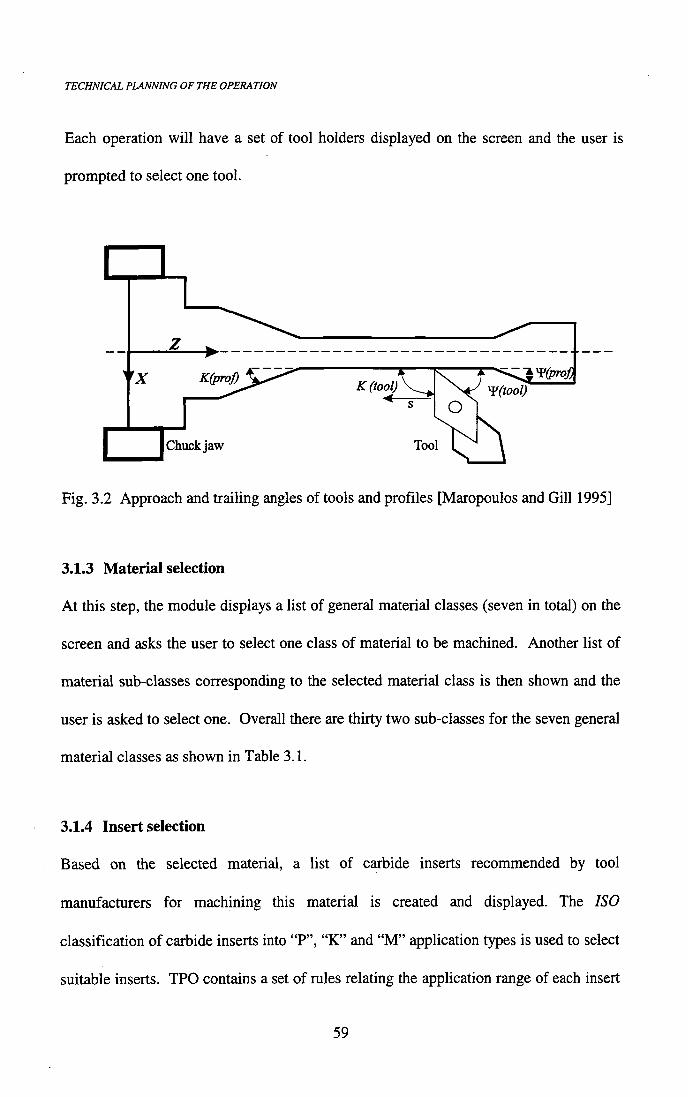
TECHNICAL PLANNING OF THE OPERATION
Each operation will have a set of tool holders displayed on the screen and the user is
prompted to select one tool.
K(prof) K(tool)
Chuckjaw
Fig. 3.2 Approach and trailing angles of tools and profiles [Maropoulos and Gill 1995]
3.1.3 Material selection
At this step, the module displays a list of general material classes (seven in total) on the
screen and asks the user to select one class of material to be machined. Another list of
material sub-classes corresponding to the selected material class is then shown and the
user is asked to select one. Overall there are thirty two sub-classes for the seven general
material classes as shown in Table 3.1.
3.1.4 Insert selection
Based on the selected material, a list of carbide inserts recommended by tool
manufacmrers for machining this material is created and displayed. The ISO
classification of carbide inserts into "P", "K" and " M " application types is used to select
suitable inserts. TPO contains a set of rules relating the application range of each insert
59
TECHNICAL PLANNING OF THE OPERATION
with a number of material sub-classes. The second consideration is to eliminate inserts which are not suitable for the selected tool holder. The only realistic way to retrieve an insert which is compatible to the selected tool holder is to match the insert's shape and cutting edge length with those of the tool holder. The ISO codes of inserts and holders can be used to automatically check whether an insert can be located on a given holder. In particular, the second character of the holder's code indicates the shape of insert and must be identical with the first character of the insert's code. Also, the last two digits of the holder's code indicate the length of the cutting edge and should match the first two digits found in the insert's code.
Example
Tool holder code: PCLNR2020-12A
Insert code: CNMGI20408-MF2
TPO matches the second character (C) and the last two digits (12) from the tool holder
code with the first character (C) and the first two digits (12) from the insert code to
ensure the same shape and size. Several inserts may be found with a suitable grade and
suitable for the selected holder. The user is required to select one from all suitable
inserts for final use.
60
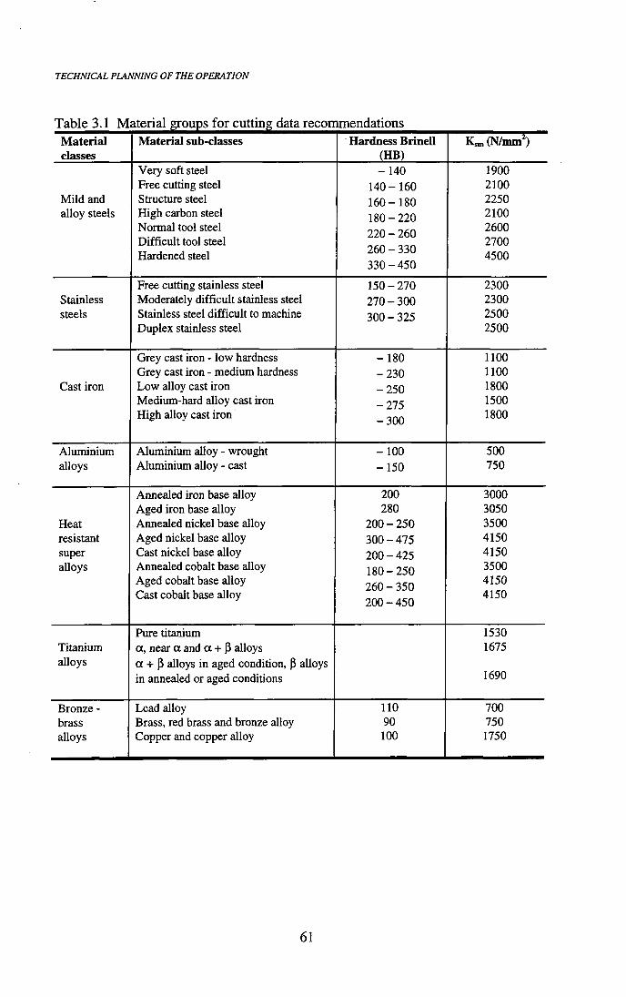
TECHNICAL PLANNING OF THE OPERATION
Table 3.1 Material groups for cutting data recommendations Material Material sub-classes Hardness Brinell K ^ ( N W ) classes (HB)
Very soft steel - 140 1900 Free cutting steel 140-160 2100
Mild and Structure steel 160-180 2250 alloy steels High carbon steel 180-220 2100
Normal tool steel 220 - 260 2600 Difficult tool steel
220 - 260 2700
Hardened steel 260 - 330 4500 330 - 450
Free cutting stainless steel 150 - 270 2300 Stainless Moderately difficult stainless steel 270-300 2300 steels Stainless steel difficult to machine 300-325 2500
Duplex stainless steel 300-325
2500
Grey cast iron - low hardness -180 1100 Grey cast iron - medium hardness -230 1100
Cast iron Low alloy cast iron -250 1800 Medium-hard alloy cast iron -275 1500 High alloy cast iron -300 1800
Aluminium Aluminium alloy - wrought -100 500 alloys Aluminium alloy - cast -150 750
Annealed iron base alloy 200 3000 Aged iron base alloy 280 3050
Heat Annealed nickel base alloy 200 - 250 3500 resistant Aged nickel base alloy 300 - 475 4150 super Cast nickel base alloy 200-425 4150 alloys Annealed cobalt base alloy 180-250 3500
Aged cobalt base alloy 260 - 350 4150 Cast cobalt base alloy 200-450 4150
Pure titanium 1530 Titanium a, near a and a + p alloys 1675 alloys a + p alloys in aged condition, P alloys
1690 in annealed or aged conditions 1690
Bronze - Lead alloy 110 700 brass Brass, red brass and bronze alloy 90 750 alloys Copper and copper alloy 100 1750
61

TECHNICAL PLANNING OF THE OPERATION
3.1.5 Depth of cut and feed rate calculations
3.1.5.1 Finishing operation
• Depth of cut
Finish machining is a single pass turning operation. Therefore, TPO will set the total
depth of cut {astock) equal to the depth of cut.
a = astock (3.1)
The depth of cut is effectively defined by the geometry of the operation and it must be
within the chipbreziker application range (i.e., acmin <acmax) (see Figure 3.3).
I f the depth of is cut less than mm. the system will set the depth of cut to be equal to
the minimum depth (a = Uc mm) and if a > Ucmax^^ depth of cut is set equal to the
maximum depth (a = ac max)- I f the user does not accept this suggestion another
chipbreaker must be selected.
E E
3 O
Q. 0) Q
^ crmix
a 1
^ cmin \
1
•J cmin Feed rate (mm/rev)
Figure 3.3 Chipbreaker application range diagram.
62

TECHNICAL PLANNING OF THE OPERATION
• Feed rate
For finishing operations the surface finish and tolerances are affected by the
combination of nose radius and feed rate as well as the workpiece stability, clamping
and the overall condition of the machine tool. The surface finish can often improve by
using higher cutting velocities and neutral or positive rakes [Sandvik Coromant 1993].
According to the surface roughness requirement (/?Q) and the selected insert nose radius
(rg), the maximum allowable feed rate can be calculated as follows [Maropoulos 1990]:
Srmax = (0-0312 r, RJ'^ (3.2)
Once the maximum allowable feed rate is computed, it will be checked against the
chipbreaker application range and the maximum feed rate is given by:
S — Sfnca — niin {Sj- f„ax > • c max)
Figure 3.3 shows the initial values of a and s which must be within the chipbreaker's
application range.
3.1.5.2 Roughing operation
• Depth of cut
The maximum depth of cut achievable by the shape of a tool holder (i.e. approach angle
and length of the cutting edge) can be calculated as follows:
2
where; Ig is the length of cutting edge and K is the tool's approach angle. The depth of
cut is set equal to this maximum value; a = a^ca = ^ r max-
63

TECHNICAL PLANNING OF THE OPERATION
This value must be within the capabilities of the given insert and the depth of cut is set equal to the maximum chipbreaking value (a = a^ax = «c max), i f max max > Or equal to the minimum chipbreaking value (a = Umax = ^cmw). i f (^tmax< ^cmin-
The number of passes (npasses) required to machine the total stock (ustock) when the
depth of cut is Umax Can be calculated as follows:
'^passes ~ stock ^ Q
V ^max J
(3.4)
The value of Upasses is rounded to the next higher integer number.
Then the final depth of cut is:
^passes
• Feed rate
The maximum feed rate for a roughing cut can be calculated using the following
empirical formula:
Srmax= 0.8 (3.6)
Initially, the feed rate is set equal to this maximum value, s = Sr max- I f - r max > - c max,
the new value is set equal to the maximum chipbreaker value (s = Smax= max) whilst,
^ ~ ^max ~ ^cmim i f ^rmax ^cmin -
The calculated depth of cut and feed rate values will be the initial cutting parameters for
a roughing operation.
64
TECHNICAL PLANNING OF THE OPERATION
3.1.6 Cutting forces
The cutting forces acting on the tool are an important aspect of machining operations.
For those concerned with the manufacturing of machine tools, a knowledge of the
cutting forces is needed for the estimation of power requirements and for the design of
structures adequately rigid and free f rom vibration. The cutting forces vary with the tool
angles and component material and accurate estimation or measurement of forces is
required in optimizing the machining conditions. For a semi-orthogonal cutting
operation in lathe turning, the cutting force can be resolved in three directions. The
component of the force acting on the rake face of the tool, normal to the edge in the
direction of cutting velocity is called the cutting velocity force component (fy). This is
usually the largest of the three force components. The force acting on the tool which is
parallel to the direction of the feed rate, is referred to as the feed force {fs). The third
force component,/a, is in the direction of the depth of cut and is the smallest of the three
force components. The velocity force component (/j,) can be calculated by using this
formula:
f , = KcorrKsm(as) (3.7)
where; Ksm is the specific resistance to cut of the material and gives the force required
for removing a chip of a cross section of 1 mm^ (Table 3.1). The Ksm value is defined
as:
K,^=^= velocity cutting force ^ ^ ^ ^ ^ . ^ 3 A chip area
65

TECHNICAL PLANNING OF THE OPERATION
The Ksm value, however, varies not only with the material properties but also depends on factors such as:
• Insert geometry.
• Entering angle of the tool.
• Feed rate.
The effect of the first two factors is diff icul t to accurately predict and is smaller than
that o f the feed rate. Therefore, TPO considers the effect of the feed rate on Ksm • The
Ksm value is corrected by using a correction factor {Kcorr) for different feed rates, ^con-
depends upon several factors such as the chip thickness and deformation energy and has
low values for high feed rates and high values for low feed rates. Table 3.2 shows the
values of Kcorr for several different feed rates [Sandvik Coromant, 1985].
Table 3.2 Kcorr Correction factors for feed rates Feed rate (mm/rev) 0.1 0.15 0.2 0.25 0.3 0.35 0.4
^corr 1.49 1.32 1.22 1.14 1.06 1.03 1.00
Feed rate (mm/rev) 0.5 0.6 0.7 0.8 1.0 1.02 1.4
^eorr 0.94 0.89 0.85 0.82 0.77 0.72 0.69
The other two force components can be calculated using a given force ratio between the
force components which is assumed to be constant and independent of the workpiece
material. However, the force ratio depends on the approach angle of the tool and varies
with the type of operation (i.e. finishing or roughing). The following ratio is used by
TPO [Maropoulos, private correspondence]:
f , : f s : f a = 4.2:2.5:1.0 (3.9)
66
TECHNICAL PLANNING OF THE OPERATION
The three calculated components of the cutting force w i l l then be calculated in order to take them into consideration for further force-related checks.
3.1.7 Force constraints
Having calculated the cutting force components acting on the cutting tool, TPO also
calculates the three maximum forces due to constraints in the three main directions,
using the fol lowing formulas [Maropoulos 1990,1991]:
a fg clmdia fvJ=^^^. (3-10)
cpdia
where; f ^ j is the maximum velocity force allowed before the workpiece starts rotating
inside the chuck, fi is the coefficient of friction (ji = 0.3), fg is the clamping force (N),
clmdia is the clamping diameter inside the chuck (mm), and cpdia is the machining
diameter (mm) as shown in Figure 3.4.
0.5 (clmlen + ^. clmdia) fg
where; /v2 is the maximum velocity force before the workpiece is thrown out of the
chuck (N), clmlen is the length of the workpiece inside the chuck (mm), cpdist is the
maximum distance of the tool f rom the face of the chuck (mm).
67

TECHNICAL PLANNING OF THE OPERATION
clmdial cpdia
^ clmlen ^!
cpdist K Figure 3.4
F ina l ly , /v j , is the velocity force which utilizes the maximum machine tool power.
^60000
^max, power
The cutting velocity Vmax,power, can be calculated f rom the formula:
K cpdia Hfnax
(3.12)
" max, power 1000 (3.13)
where; Pmax is the maximum machine power (N), and rimax is the maximum spindle
speed (rpm) for maximum power as shown in Figure 3.5. For most machine tools,
maximum power is obtained over a range of spindle speed and Figure 3.5 shows the
capability of the CNC-1000 lathe which was used in the experimental work. Using the
maximum spindle speed in equation 3.13 results in high values for Vmax.power which in
turn reduces the/vj value.
68

TECHNICAL PLANNING OF THE OPERATION
7.5
1 o.
P(max)
j n (nin)
1 200 Speed (rev/m in) 3,750
Figure 3.5 Power-speed diagram of the machine tool CNC-1000
For turning operations, the velocity cutting force ( f j must be less than the minimum
constraint force in the velocity direction,/v;, /v2, and/v j .
/v < min ( f y ] , /v2 ,fv3) (3.14)
I f this check fails, TPO w i l l set:
fv,new = rnin (fvl, fv2, fvS)
Initially, it is attempted to obtain the reduced velocity force component by reducing the
feed rate for the same depth of cut.
fv, new ^new
^corr ^sm ^ (3.15)
The feed rate can be reduced up to the minimum chipbreaking value {Sc min)- When s^w
< Sc min, the depth of cut should be reduced by increasing the number of passes by one
and resetting the feed rate to its initial value.
^passes.new — ^passes 1 (3-16)
69

TECHNICAL PLANNING OF THE OPERATION
and
« « e w = ^ ^ ^ ^ (3.17) ^passes,new
The above process w i l l be repeated until the condition in equation (3.14) is satisfied.
• Axial and radial force constraints
The maximum axial force before the workpiece starts sliding in the chuck is calculated
as follows:
faxial = f l f g (3-18)
where; faxial is the maximum axial force to prevent axial slip of the workpiece in the
chuck (N).
The cutting force deflects the workpiece and in the case of single point workholding, the
maximum radial force fradiai allowed can be calculated as follows:
/ . » . ^ , = (N) (3.19) cpdist
where; defcom= —(diametral tolerance) 2
64
where; E is Young's module of elasticity. The diametral tolerance is set by default to
0.03 mm. The user can specify any other value.
70

TECHNICAL PLANNING OF THE OPERATION
For longitudinal operations, the feed force {fs) and the force acting in the direction of depth of cut (fa) calculated by equation 3.9, should be less than or equal to the calculated axial force (faxiad and radial force ( fradiad respectively.
fs axial
and
fa —fradial
For facing operations the direction of the cutting force fs and fa is reversed and the
system w i l l check the f o r c e t o be less than or equal to the axial force constraint (faxiad,
and the feed rate force (fs) to be less than or equal to the radial force constraint/^o^ja/.
fs ^fradial
and
fa —faxial
I f the last two checks fa i l , the system w i l l reduce the value of the feed rate and of the
depth of cut as described in the case of the velocity force. A t the end of this process all
force related constraints have been satisfied and the values of depth of cut (a) and feed
rate (s) are accepted as feasible cutting conditions.
3.1.8 Cutting velocity
Based on the type of cut (finishing, medium roughing or roughing operation), TPO
shows the user a range of cutting velocities reconmiended by tool manufacturers to cut
71

TECHNICAL PLANNING OF THE OPERATION
the selected material sub-class by the selected grade. The user is required to select a value of cutting velocity (v).
• Rotational speed check
The spindle speed corresponding to the selected value of cutting velocity can be
calculated f rom the following formula:
n = — (rpm) (3.21)
K D
The rotational speed (n) should be within the speed range of the selected machine (n^^ /n
< n < r i f f i ^ ) as shown in Figure 3.5. I f it is less than the machine minimum the
calculated value w i l l be set equal to the minimum ( n = ^ it is greater than the
maximum machine speed the calculated rpm value w i l l be reduced to the maximum
spindle value (n = n»iax)- ^ tiew sub-optimal cutting velocity (v) w i l l then be calculated
using equation (3.21).
• Power check
The power required for metal cutting is mainly of interest during roughing, when it is
essential to ensure that the machine has sufficient power for the operation. The basic
parameters in the power calculation are the rotational cutting force velocity, f y , and the
cutting velocity (v). The efficiency factor of the machine is also important. The
efficiency factor (rj), depends on the type of transmission the machine is fitted with, and
the overall machine condition. The machine efficiency is normally between 0.6 to 0.9,
72

TECHNICAL PLANNING OF THE OPERATION
and r\ = 0.75 is used within the system. The required power can be calculated as follows:
Power = (Kw) (3.22) 60000T]
The calculated power should be less than or equal to the maximum machine power (P <
Pmachine)- I f this test fails, the power w i l l be set equal to the maximum machine power
and the final cutting velocity can be recalculated using equation (3.22). After the
execution of the algorithm described above the three cutting parameters (a, s and v) of a
machining operation have been calculated.
73
Chapter 4
TOOL L I F E PREDICTION
This chapter describes the tool l i fe prediction (TLP) module. The first task of any
computer-based system is to define the problem the user is trying to solve. TLP
accomplishes this through a series of interactive decision trees in which the user
specifies interactively the characteristics of the required machining operation by
selecting a component using the appropriate user interface window. A number of
operations (up to 5 operations) are displayed on the screen and the user must select one
operation. The essential information required by TLP is in relation to the cutting
conditions (cutting velocity and feed rate), tool code, insert grade, type of cut, type of
cutting fluid, machine tool and the material class and sub-class. The technical planning
of an operation creates most of this information as described in Chapter three.
However, at this level there is a need to re-confirm certain elements of the operation
which have a direct influence on tool l i fe . The workpiece material and tool's carbide
grade belong to this category.
To describe a work material, the user chooses from a list of material classes (mild and
alloy steels, stainless steels, cast iron, aluminium etc.) as shown in Table 3.1. Within the
general material class there are usually several sub-classes, for example, for stainless
steel there are free-cutting stainless steel, moderately difficult to cut stainless steel or
di f f icul t to machine stainless steel. The user selects a sub-class and based on the chosen
74
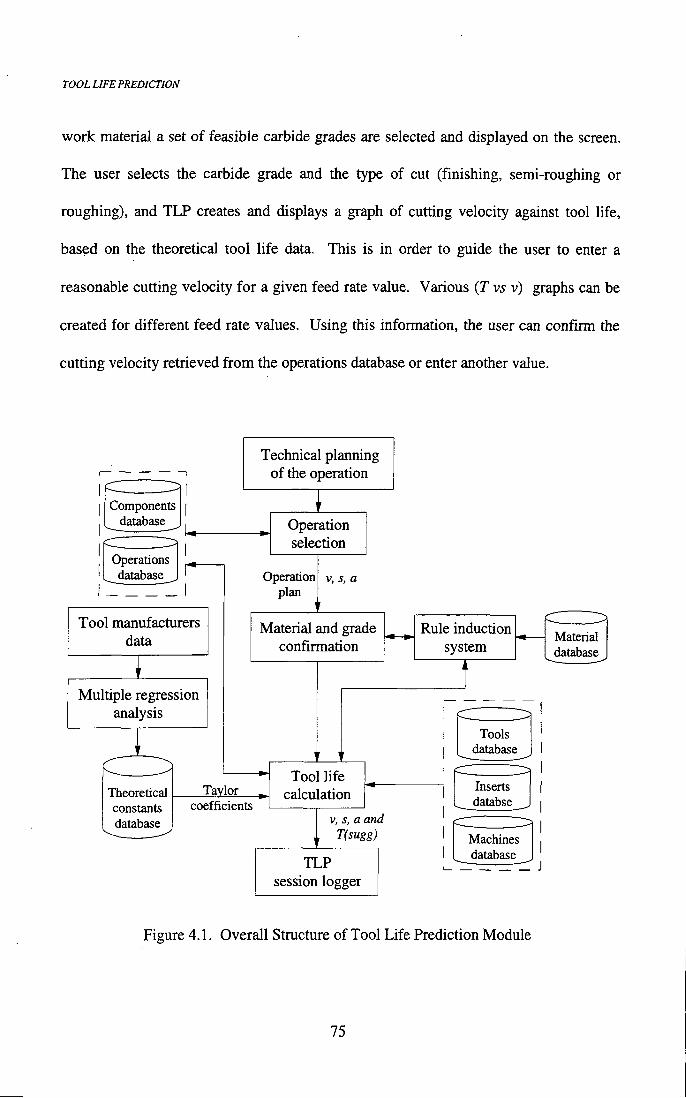
TOOL LIFE PREDICTION
work material a set of feasible carbide grades are selected and displayed on the screen. The user selects the carbide grade and the type of cut (finishing, semi-roughing or roughing), and TLP creates and displays a graph of cutting velocity against tool l i fe, based on the theoretical tool l i fe data. This is in order to guide the user to enter a reasonable cutting velocity for a given feed rate value. Various {T vs v) graphs can be created for different feed rate values. Using this information, the user can confirm the cutting velocity retrieved f rom the operations database or enter another value.
Components database
Operations database
Tool manufacturers data
Multiple regression analysis
Theoretical constants database
Technical planning of the operation
Operation selection
Operation plan
V, s, a
Material and grade confirmation
Taylor coefficients
Tool l i fe calculation
V, s, a and T(sugg)
TLP session logger
Rule induction system
1
Material database
Tools database
Inserts databse
Machines _jatabase ^
Figure 4.1. Overall Structure of Tool Li fe Prediction Module
75

TOOL LIFE PREDICTION
The tool l i fe value predicted by TLP is used as an initial recommendation based on theoretical data and is later considered by the tool l i fe assessment module of the system. Figure 4.1 shows the structure of TLP and a more detailed description of its functionality follows.
4.1 AUTOMATIC RULE INDUCTION SYSTEM
The automatic rule induction system is a front-end system to Crystal. It w i l l
automatically turn a table of material values such as the chemical percentage
compositions for a number of materials within each material sub-class, into a well
structured set of Crystal rules which describe the relationship between the given values.
The Crystal induction system creates rules which are used for defining the material sub
class of a new material f rom its percentage chemical composition. The rules for each
sub-class are robust because in the tool l i fe control system there are seven main material
classes based on tool manufacturers data (Table 3.1) and each material class is further
sub-divided into several sub-classes (32 in total). The Crystal induction system looks for
attributes that split each of these material sub-class and creates rules automatically f rom
these examples which define the composition limits of each material sub-class. The
rules created by the induction system are well structured and easily extendible within the
Crystal program.
The chemical percentage composition and the Brinell hardness for all the material sub
classes within each material class were collected [Metcut Res. Assoc. 1980; Wegst
1992; Soc. Auto. Engs. 1981] and fed into the rule induction system to generate rules
76

TOOL LIFE PREDICTION
and conditions which define the limits of each sub-class. Table 4.1 shows the chemical composition of the iron base alloy sub-class material of the heat-resistant super alloy class.
Table 4.1 shows fourteen materials belonging to this sub-class. The complexity of the
information is apparent since there are eleven alloying elements. This table is processed
by the rule induction system and a complex rule concerning the chemical composition of
all members of this sub-class is constructed.
Table 4.1 Chemical percenta: ge composition of some iron alloy base sub-class materials USA UK Fe Ni Co Cr Mo w Si Mn c AI TI
ASTM: 638 HR5152 53.65 26.0 - 15.0 1.3 - 0.5 1.3 0.05 0.2 2.0
ATM: A638 54.26 26.0 - 13.5 27 - 0.8 0.9 0.04 0.1 17
5725 50.53 25.0 - 16.0 6.0 - 0.7 1.35 0.12 - 0.3
AISI: 615 80.98 2.0 - 13.0 0.15 3.0 0.3 0.4 0.17 - -
5768 33.40 20.0 20.0 21.0 3.0 2.5 - - 0.1 - -
ASME ; SB 163 3082-76 44.85 32.5 - 21.0 - - 0.5 0.8 0.05 0.4 0.4
5552 45.05 32.0 - 20.5 - - 0.5 0.8 0.05 - 1.1
3072-76 41.64 37.0 - 18.0 - - 2.3 1.0 0.06 - -
5718/9 83.65 2.5 - 12.0 17 - - - 0.15 - -
5768 31.35 20.0 20.0 21.0 3.0 2.5 0.5 1.5 0.15 - -
5533 30.57 20.0 20.0 21.0 4.0 4.0 - - 0.43 - -
AISI: 663 52.57 27.0 - 14.8 1.25 - 0.75 0.3 0.08 0.25 3.0
AISI: 665 53.97 26.0 - 13.5 1.5 - 0.4 1.5 0.08 0.2 2.85
ASTM: A477 68.0 9.0 - 19.0 1.0 1.0 0.6 1.1 0.3 - -
77
TOOL LIFE PREDICTION
The rule created by the induction system for defining the iron base alloy sub-class
material within the heat resistance super alloy class is as follows:
IF Cu is less than 42.950
A N D N i is less than 34.000
A N D Co is less than 29.000
A N D T i is less than 37.825
A N D NOT Fe is less than 15.225
OR Cu is less than 42.950
A N D NOT N i less than 34.000
A N D NOT C is less than 0.020
A N D N i is less than 49.050
A N D NOT Fe is less than 38.470
The user can induce the use of the rule induction system by selecting the "Unknown"
option when asked to select f rom the material sub-class list in the Crystal program. The
user is prompted to supply information concerning the material chemical composition
and/or its Brinell hardness range. Then the rule induction system can define the sub
class of the user defined material as described above. Having defined the sub-class,
TLP retrieves the theoretical constants for the calculation of tool l ife.
4.2 CALCULATIONS OF THE THEORETICAL TOOL L I F E CONSTANTS
F. W. Taylor (1907) was the first to investigate the relationship between tool l ife and
cutting conditions such as cutting velocity, feed rate and depth of cut. A database of
78

TOOL LIFE PREDICTION
tool supplier's cutting conditions and tool l ife data [Sandvik Coromant 1993; Seco Tools 1993] for a wide range of carbide tools and different workpiece materials, was analyzed using multiple regression to calculate the theoretical coefficients of the extended form of ray/or'^ equation (/nC, ^ > ) -
Equation 4.1 does not directly include the influence of depth of cut. This is
incorporated in the constant C. The tool l i fe coefficients are calculated for the three
types of operations namely, finishing, medium-roughing and roughing. Appendix. 2
shows the fo rm of the input data tables, relating a carbide grade to a material sub-class
for finishing, medium roughing and roughing operations. The cutting data shown in
Appendix 2 w i l l result in tool l i fe of approximately 15 minutes, but this is dependent on
other factors such as chipbreaker type, set-up stability of the part, machine tool
condition, stability of the tool and tool overhang. Tool manufacturers advise that to
achieve longer tool l i fe , one should multiply the recommended cutting velocities by the
fol lowing simplistic empirical factors:
Target Tool Life Velocity (min) Factor
30 0.86 45 0.79 60 0.74
These simple, empirical factors were used to create additional sets of cutting data and
tool l i fe and calculate initial values for the tool l i fe constants. The initial clustering of
79

TOOL LIFE PREDICTION
tool l i fe predictions induced by applying these simple factors is eliminated by applying a continual feedback process by collecting and processing real tool l i fe values f rom the shop floor.
Mult iple regression techniques allow the calculation of the tool l i fe coefficients as
shown in Appendix 3. The coefficients are stored in the tool l ife constants database and
are subsequently used to predict tool l i fe . Table 4.2 shows the calculated tool l ife
constants for machining free cutting steel (EN8) using TP 10 and TP20 insert grades
under finishing, semi-roughing and roughing cutting conditions as well as for machining
di f f icul t stainless steel (SS 316) using TP35 insert grade. The details of using the
multiple regression method to calculate the coefficients of the linear form of Taylor's
tool l i fe equation are described in the next section.
Table 4.2 Tool l i fe constants calculated 5y multiple regression
Material sub-class Insert
grade
Type of cut In C 1/a 1/P
TPIO Finishing 29.690 4.584 0.298
Semi-roughing 23.015 3.446 0.000
Roughing 22.847 3.478 0.000
Free cutting steel TP20 Finishing 29.072 4.612 0.292
Semi-roughing 25.600 4.531 2.596 it Roughing 23.987 4.309 2.503
Difficult stainless steel TP35 Finishing 14.609 2.548 0.060
Semi-roughing 21.501 4.307 0.000
80

TOOL LIFE PREDICTION
4.2.1 Multiple Regression
Multiple regression takes into account the effect of more than one independent variable,
such as cutting velocity (v) and feed rate (5), on the dependent variable which is tool life
(7) [Wonnacott 1990]. The relationship between the dependent variable T and the two
independent variables v and s in the linear form is:
lnT = lnC + i - l / a ) Inv + (-1/^) Ins (4.2)
Different v, and j / result in different T, and equation 4.2 will have the form:
A
lnTi=lnC + (-1/a ) In + ) In Si (4 3)
A
In 7} is the expected value of InTf. The difference between the observed and expected
values of InTi is the stochastic error term (60. Thus, any observed value InTi may be
expressed as its expected value plus this disturbance term.
lnTi=lnC + (-1/a ) Invi + ( - l / p ) Insi +ei (4.4)
The Least Squares method is driven by selecting the estimates of InC, , that
minimize the sum of the squared deviations between the observed and the estimated
values of InT; that is, minimize:
i2 ^ / \ A
InTi - IriC - {-^) Invi - ( - j ) Insi (4.5)
^ A A
where; InC, , are the estimated values of InC, ^ • This is done by setting
the partial derivatives of the above function with respect to InC, , equal to zero.
This gives the following three equations:
81

TOOL LIFE PREDICTION
X[ ( InVi -Inv) [inTi - In t ) =
a >* X « - « ] ^('i ^Y. [(^"^j - « - ^ ) ] (4.6)
A A
( - i ^ « ^ ^ - - l n v ) [ l n s i - l n s ) ] + ( - j Inst-lns] (4.7)
A ^ ^
C = / « r - ( - ^ ) l n v - ( - j ) Ins (4.8)
Appendix 4 shows these calculations for TP20 insert grade when cutting free-cutting
steel material under medium roughing machining conditions.
4.3 T O O L L I F E C A L C U L A T I O N C R I T E R U
The prediction module has access to seven databases namely, tools, inserts, machines,
material, theoretical tool life constants and the approved database as shown in Figure
4.1. The first three databases are essential for reading information such as cost,
chipbreaking range, machine power and speed range in order to calculate the overall
machining constraints. The material properties database is used by the rule induction
system to define the material sub-class of a user defined material. For the same insert
grade, workpiece material and type of cut, TLP retrieves the tool life coefficients from
the f i f th database (constants database) and calculates the theoretical tool life value. The
prediction module calculates the tool life value according to the following criteria:
• Tool life for user defined cutting conditions.
82

TOOL LIFE PREDICTION
• Tool life for minimum production cost.
• Tool life for minimum production time.
4.3.1 Tool life for user deHned cutting conditions
For any given cutting conditions (v and s), the tool life is calculated using the linear
form of Taylor equation.
In Ti = InC + (-l7a ) In v,- + (-l7p ) In Sj (4.9)
The relationship between cutting data and tool life can be used for optimising the
economics of the cutting process. Two distinct criteria can be used for choosing the
cutting velocity for a machining operation; minimum production cost and minimum
production time.
4.3.2 Tool life for minunum production cost
The time spent by the operator in producing w batches of size q can be separated into
three items:
w qtj = Work set up time, where t] is the time taken to load and unload each
component.
w q = Machining time, where t2 is the machining time.
Ne = Tool changing time, where is the time to change an individual tool and A ^ is
the number of cutting edges used. At this stage it is assumed that Ng is equal
to the number of machine stops for tool changing.
83

TOOL LIFE PREDICTION
Thus, i f X is the total machine and operator rate (including overheads), the total machine and operator costs will be:
x(wqtj + wqt2 + Net3) (4.10)
This cost must be added the cost of the tool used, Ne y , where y is the cost per cutting
edge. The average production cost, Cpr, for each component is:
Cpr = xti+xt2 + [Ne/(wq)]xt3 + [Ne/(wq)]y (4.11)
The first term in this equation is the non-productive cost due to work set up which is
constant for the particular operation. The second term is the machining cost, which
reduces as the cutting velocity increases at constant feed rate. The final two items are
giving the tool costs, which increase as the cutting velocity increases. Figure 4.2, shows
the empirical relationship between the cutting velocity and the tool life [Taylor 1907]:
— = ( —1 Vr \T J
(4.12)
where; v is the cutting velocity; T is the tool life; a is constant, and TV is the measured
tool life for a given cutting velocity v -.
84
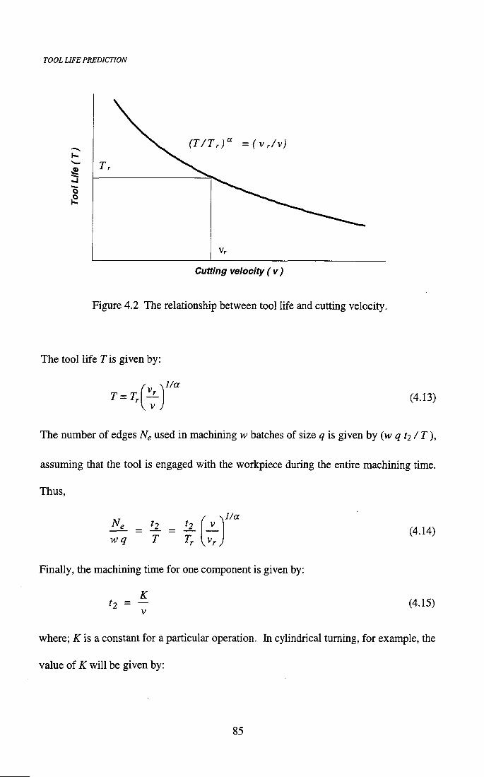
TOOL LIFE PREDICTION
(T/Tr)" = i V r / v )
Cutting velocity ( v )
Figure 4.2 The relationship between tool life and cutting velocity.
The tool life Tis given by:
T = T, V V
(4.13)
The number of edges Ng used in machining w batches of size q is given by (w q t2 / T),
assuming that the tool is engaged with the workpiece during the entire machining time.
Thus,
w q T
1/a
(4.14)
Finally, the machining time for one component is given by:
K h = - (4.15)
where; is a constant for a particular operation. In cylindrical turning, for example, the
value of K wil l be given by:
85

TOOL LIFE PREDICTION
K = K Dl
(4.16)
In general, K can be regarded as the distance moved by the cutting edge relative to the
workpiece during the machining operation.
The relationship between the production cost and the cutting velocity can be obtained by
substituting equations (4.14) and (4.15) in equation (4.11).
Cpj. = xtj + xKv'^ + K
( x f j +3.)v(^-«)/« (4.17)
To find the cutting velocity (Vmc) for minimum cost, equation (4.17) must be
differentiated with respect to v and equated to zero. Thus;
a xTr .a
l - a xt^+y (4.18)
By substituting equation (4.18) into equation (4.13), the optimum tool life for minimum
cost (Tmc) is:
l-afxt^ + y
a (4.19)
The cost per cutting edge (y) for an indexable insert can be calculated as follows
[Maropoulos and Hinduja 1990]:
Insert cost 1.3 x Holder cost y = 0.75 X number of cutting edges + 400
(4.20)
86

TOOL UFE PREDICTION
4.3.3 Tool life for minimum production time
To find the optimum cutting velocity for maximum production rate (or minimum
production time) v^t, it is necessary to follow a similar procedure to that described in
section 4.3.2. The average production time for one component is given by:
tpr = tj + t2 + -^ts (4.21) w q
Substitution of equations (4.14) and (4.15) in equation (4.21) and differentiation gives
the cutting velocity (Vmt) for minimum production time.
1-a ts (4.22)
The optimum tool life for minimum production time (T^^) can be obtained by
substituting equation (4.22) in equation (4.13).
(4.23) 1 - a\
a J
Finally, the cutting velocity (v) and the spindle speed (n) are calculated using Taylor's
tool life equation (4.1).
r c ^"
1000 V n = • K D
where, D is the effective (generated) machining diameter (mm).
(4.24)
(4.25)
87

TOOL LIFE PREDICTION
The calculated spindle speed should be within the rotational speed range of the selected machine as described in Section 3.1.8. I f the rotational speed (n) must be modified, new cutting velocity is obtained using equation 4.25.
The results from TLP are displayed on the results screen, together with a question
asking whether they are acceptable. I f the user replies "NO", TLP restarts the process
for calculating the tool life with different options given by the user. I f the user answers
"YES", the results will be saved automatically in the TLP session logger. Then the user
can decide whether the results should also be saved in the system's database. A number
of results can be stored temporarily in the session logger when the user wishes to
continue with the assessment of those predictions using approved information as will be
described in Chapter 6. The TLP session logger is a dynamic file created by the module
in order to save the TLP calculation for the operation under consideration. Up to ten
operations can be saved in the session logger file.
The session logger can be accessed from the next module of the system, the tool life
assessor TLA. Any operation can be selected from the session logger to be considered
as an input for TLA.
88
Chapter 5
INITIAL TOOL LIFE TESTS
A series of experiments were designed and completed to test the accuracy of the
theoretical tool life predictions. The cutting tests were carried out by turning free
cutting steel (ENS) and difficult to machine stainless steel (316) using three different
coated carbide grades (TPIO, TP20, and TP35). The calculation of cutting conditions
was based on the algorithmic method implemented in the technical planning module
(TPO). The suggested tool life values (Tsugg) predicted by TLP were based on the
theoretical tool life constants generated by multiple regression as shown in Table 4.2 in
Chapter 4. The main objectives for the initial experimental work were:
• To establish the effect of cutting conditions on tool life for different insert
grades, workpiece materials and types of cut.
• To study the relationship between the flank wear rate and machining time.
• To validate the operation of the first two modules namely, TPO and TLP, in
relation to their main functions.
• To build the approved tool life history which will be used by the tool life
assessor module (TLA).
89

INFTIAL TOOL LIFE TESTING
5.1 APPARATUS USED 5.1.1 The centre lathe
The Colchester CNC-1000 centre lathe shown in Figure 5.1 was used for the tests. The
CNC-1000 was specifically designed for jobbing shops and tool rooms and has a
maximum power of 7.5 kW (30 minute rated), whilst its maximum power for constant
operation is 5 kW. The maximum spindle speed is 3750 rev/min as shown in Figure
3.5. This lathe has a robust headstock design with a heavy-duty precision spindle that
offers high radial load capacity and guarantees roundness accuracy better than 2 |jm.
Figure 5.1 Colchester CNC-1000 centre lathe
90

INITIAL TOOL LIFE TESTING
5.1.2 Tool holder and inserts
The tool holder geometry for the tests was the widely employed PCLNR2020-12A and
the carbide inserts had nose radii of 0.4 and 0.8 mm as shown in Figure 5.2. Three types
of carbide grades were tried (TPIO, TP20 and TP35), corresponding to the ISO PIO, P20
and P35 application ranges. The chipbreaking geometries employed were suitable for
light to medium roughing machining operations. The chipbreaking geometry employed
with TPIO and TP20 insert grades when finish machining free cutting steel (ENS) was
MF2. MF2 limits the depth of cut in the range between 0.5 and 3.5 mm and the feed
rate between 0.1 and 0.4 mm/rev. The MF3 chipbreaker was used on TP20 and TP35
insert grades to cut free cutting and difficult stainless steel (316) respectively. The
application range of MF3 limits the depth of cut between 1 and 4 mm and the feed rate
between 0.1 and 0.4 mm/rev.
Figure 5.2 PCLNR-2020_12A and the carbide inserts used in the initial tests.
91

INTTIAL TOOL LIFE TESTING
5.1.3 Workpiece material
Two types of workpiece materials were used for the tests. The first workpiece material
was BS080A40 (ENS) free cutting steel and its specific resistance to cut is
approximately 2100 N/mm^ depending on the feed rate used. The second type of
workpiece material was (SS316), which is difficult to machine austenitic stainless steel
and its specific resistance to cut is approximately 2500 N/mm^. Free cutting steels are
produced with additions of 0.1% to 0.3% sulphur or 0.3% to 0.35% lead or
combinations of both to reduce cutting forces, cutting temperature and hence tool wear
rates. These additions allow, for the same wear rate, higher cutting velocities to be
applied with improved surface finish. Austenitic stainless steels have high work-
hardening rates and low thermal conductivity. Their high work-hardening rate causes
high energy consumption. The low thermal conductivity causes high temperature
gradients within the chip. The high temperatures in the chip-tool interface result in
increased diffusion wear rates.
5.1.4 Measuring microscope
The Carlzeiss Jena 10907 toolmaker's microscope shown in Figure 5.3 was used in
these tests. It is equipped with micrometer screws which perform the double function of
moving the table laterally and horizontally and provide measurements to the accuracy of
0.0001 in (0.00254 mm). The most common method of measuring is by the .use of
graticule hair lines. The edge of the part to be measured is lined up with the hair line.
At that point, a zero setting can be made on the micrometer dial. The part is then moved
until its other edge is lined up with the hair line and the distance noted on the dial.
92

INTTIAL TOOL LIFE TESTING
Figure 5.3 Carlzeiss Jena 10907 microscope used for measuring the flank wear
5.2 TOOL FAILURE CRITERIA
The wear of the face and flank of the cutting tool is not uniform along the active cutting
edge. Therefore, it is necessary to specify the locations and the degree of wear when
deciding on the amount of wear allowable before replacing the cutting insert. The
criteria recommended by the International Standards Organisation (ISO) dealing with
tool life testing follow [ISO 3685-1977]:
93

INTTIAL TOOL UFE TESTING
• High speed steel or ceramic tools
The failure criteria which give the effective tool life for high speed steel or ceramic tools
are:
• Catastrophic failure.
• V B = 0.3 mm i f the flank is regularly worn.
VBinax = 0.6 mm i f the flank is irregularly worn, scratched, chipped, or badly
grooved.
• Sintered carbide tools
One of the following failure criteria is recommended:
• V B = 0.3 mm.
VBmax = 0.6 nun i f the flank is irregularly worn.
• KT = 0.06 + 0.3 5 , where s is the feed rate.
VB(max)
Figure 5.4 The way of measuring tool wear
94

INITIAL TOOL UFE TESTING
For this testing phase, a wear land of approximately 0.35 mm was taken as the failure criterion. The reason for setting this criterion was that the measurement of wear was not continuous but instead wear was measured at discrete intervals. In each case a tool was considered to have failed when the measured wear {VB) exceeded 0.3 mm, and in most tests the maximum wear land measured was in the range 0.3 - 0.35 mm.
For each test, machining was interrupted after 1-3 minutes in order to measure the size
of the flank width VB; i.e. the distance between the straight part of the original major
cutting edge and the boundary of the flank wear land as shown in Figure 5.4. This
machining time interval (1-3 min) is chosen in order to monitor any change in the rate
of creation of the flank wear by taking the exact reading of the flank wear at regular
intervals.
5.3 T H E O R E T I C A L CALCULATIONS AND RESULTS
The carbide tool life data include four separate sets of cutting conditions. The cutting
conditions were calculated using the technical planning of the operation module (TPO)
and they were within the range of cutting conditions suggested by tool manufactures as
shown in Appendix 2. The initial cutting conditions calculated by TPO and the
theoretical tool life values predicted by TLP were tested on the CNC-1000 machine tool
and the final, approved results were derived. Al l cutting tests were lubricated by using a
continuous flow of a general-purpose cutting fluid (Rocol-Ultracut 370). The approved
results were then stored in the system's operations database and formed the essential
95

INTTIALTOOL LIFE TESTING
information on which the performance of the tool life assessor (TLA) was evaluated as wil l be discussed in the next Chapter.
5.3.1 Results from machining free cutting steel (ENS) using TPIO insert grade
The first set of 4 tests were obtained by cutting free-cutting steel (ENS) using a TPIO
insert grade under finish-machining conditions. The calculated cutting conditions and
the suggested tool life values predicted by TLP using the theoretical tool life constants
(Table 4.2, Chapter 4) for these tests are shown in Table 5.1.
The required surface roughness {R^ varied between 0.5 | im to 1.7|im, to check the TPO
module's functionality for calculating cutting conditions which result in different
surface roughness values.
Table 5.1 Finish machining of ENS free-cutting steel with TPIO grade. Machine Tool CNC-1000 Tool Holder PCLNR2020 12A Insert Type CNMG120408 MF2 Insert Grade TPIO (PIO) Workpiece Dimension Length=200 mm and Diameter=100 mm Cutting Fluid Rocol-Ultracut 370
Test No. Testl Test 2 Tests Test 4 Cutting Depth (mm) 1.3 1.5 1.0 1.5 Parameters Feed (mm/rev) 0.15 0.1 0.2 0.18
Velocity (m/min) 415 450 400 460 Tool Life Tsugg (min) 13.76 10.71 14.95 8.13
Surface Roug. Ra im) 0.95 0.5 17 1.3
96

INITIAL TOOL UFE TESTING
Figure 5.5 shows the progress of flank wear with machining time for four TPIO indexable inserts when finish machining ENS. The first three tests revealed similar wear rate characteristics. The wear rate in the fourth test had a constant rate for the first 5 - 6 minutes and then increased rapidly with cutting time as shown in Figure 5.5. This higher wear rate can be attributed to the combination of high velocity and high feed rate used in this test. Pictures of some inserts used in these tests are shown in Appendix 5A.
0.4 T
0.3
E E
S 0.2
c CO
0.1
Test 4 Test 2
Test 1 ^ •
y : Tests
/
-+-
0 2 4 6 8 10 12 14 16 18
Machining Time (min)
Figure 5.5 Progress of flank wear with time when finish turning ENS with TPIO.
The predicted tool life values using the theoretical tool life constants shown in Table 4.2
are in good agreement with the real, approved values observed in the experiment as
shown in Table 5.2. In two tests the theoretical tool life values were higher than those
achieved whilst in the other two tests the tool lasted longer than predicted.
97

INITIAL TOOL UFE TESTING
Table 5.2 Tsugg and Tgpp when finish machining ENS using TP 10 Test number Testl Testl Tests Test 4
Tsugg (min) 13.76 10.71 14.95 8.13
Tapp (min) 12.08 12.67 16.05 7.7
T
T
114% 85 % 93 % 106%
5.3.2 Results from machining free cutting steel (ENS) using TP20 insert grade
The cutting conditions used in these 4 tests to cut ENS free cutting steel material using
TP20 insert grade under finish machining conditions are shown in Table 5.3 together
with the tool life values predicted by TLP using the theoretical constants. The surface
roughness for these finishing tests varied between Ijam to 1.7|im. It must be noted that
in these four tests the feed rates were higher and the velocities lower than the values
used in the first series of tests. The reason is that TP20 is tougher but less hard than
TP 10 hence is withstands higher forces (increased feed) and lower cutting temperature
(reduced velocity).
Table 5.3 Finish machining of ENS free-cutting steel with TP20 grade. Machine Tool CNC-1000 Tool Holder PCLNR2020_12A Insert Type CNMG120408_MF2 Insert Grade TP20 (P20) Workpiece Dimension Length=200 mm and Diameter=100 mm Cutting Fluid Rocol-Ultracut 370
Test No. Testl Test 2 Tests Test 4 Cutting Depth (mm) 1.5 1.1 1.5 0.7
Parameters Feed (mm/rev) 0.25 0.19 0.2 0.23 Velocity (m/min) 375 390 395 450
Tool Life Tsuee (min) 8.51 7.7 7.15 3.76
Surface Roug. Ra ( lm) 1-7 1.0 1.1 1.4
98

INITIAL TOOL LIFE TESTING
The progression of flank wear with machining time when finish machining ENS free-
cutting steel with TP20 insert grade is shown in Figure 5.6. As a result of these four
tests, the tool life criterion of VBmax = 0.35 mm was reached after only 3.8 min with
cutting velocity of 450 m/min and feed rate of 0.23 mm/rev (see test 4). This means that
it is not practical to use a TP20 carbide grade at this velocity and feed range when
machining free cutting steel material. The second test shows an early start of the
accelerated wear region. This may be due to a degree of "rubbing" during the process
because of the relatively small value of the depth of cut (1.1 mm) which is only
marginally larger than the tool's nose radius (O.S mm). Pictures of some inserts
employed in this set of tests are shown in Appendix 5B.
0.4
0.3
E E
S 0.2
C «
0.1
Test 4 Test 2
Testl Tests —t
/
4 6 8 10
Machining Time (min) 12 14
Figure 5.6 Progress of flank wear with time when finish turning ENS with TP20.
99

INITIAL TOOL UFE TESTING
The tool life values suggested by TLP are again very close to the approved values
obtained from the experiment except in the third test as shown in Table 5.4. This might
be attributed to the fact that the tool manufacturer's recommendations are conservative
and also in the particular test the stability of the operation was very good with a positive
effect on tool life.
Table 5.4 Tsugg and Tgpp when finish machining ENS using TP20 Test number Testl Test 2 Tests Test 4
Tsugg (min) 8.51 7.7 7.15 3.76
Tapp (min) 9 7.58 12.5 3.8
T -^xlOO% T
95 % 102% 57 9r 99%
The suggested tool life values and the corresponding cutting conditions employed in 4
semi-roughing tests, in which free cutting steel material was machined using a TP20
insert grade are shown in Table 5.5. The calculated machine power values for all tests
are in the range of 5 kW and the spindle speed is approximately in the middle of the
machine tool's capability in order to avoid vibrations and workpiece deflection which
might affect the overall testing results. It can be seen that the suggested tool lifes are
higher than those shown in Table 5.4 and this is mainly due to the use of lower cutting
velocities.
100

INITIAL TOOL LIFE TESTING
Table 5.5 Medium-roughing machining of ENS free-cutting steel with TP20 grade. Machine Tool CNC-1000 Tool Holder PCLNR2020_12A Insert Type CNMG12040S_MF3 Insert Grade TPIO (PIO) Workpiece Dimension Length=200mm and Diameter=100 mm Cutting Fluid Rocol-Ultracut 370
Test No. Testl Test 2 Tests Test 4 Cutting Depth (mm) 2.0 2.0 1.7 1.6
Parameters Feed (mm/rev) 0.2 0.2 0.25 0.28 Velocity (m/min) 350 330 310 295
Tool Life Tsusg (min) 25.43 33.2 24.69 23.03
Mach. Power P (kW) 5.693 5.368 5.0 4.846
Spindle Speed rpm (rev/min) 1857.75 1751.59 1495.85 1381.6
Figure 5.7 shows the progress of flank wear with machining time for these tests. It is
shown that the rate of flank wear for the third and fourth tests increased rapidly with
machining time. This can be attributed to the combination of high feed rates and high
cutting velocities. Again, pictures of some inserts are shown in Appendix 5C.
0.4 T
0.3 I E E
S 0.2
C n
0.1
Test 3 Test4 ( Testl # » j e s t l
* • •
' * *
10 • 15
Machining Time (min) 20 25
Figure 5.7 Flank wear with time for semi-roughing turning ENS with TP20.
101
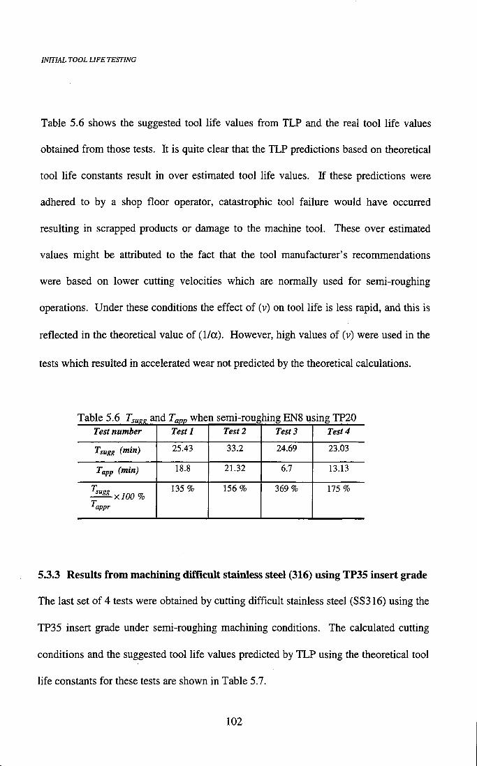
INITIAL TOOL LIFE TESTING
Table 5.6 shows the suggested tool life values from TLP and the real tool life values
obtained from those tests. It is quite clear that the TLP predictions based on theoretical
tool life constants result in over estimated tool life values. I f these predictions were
adhered to by a shop floor operator, catastrophic tool failure would have occurred
resulting in scrapped products or damage to the machine tool. These over estimated
values might be attributed to the fact that the tool manufacturer's recommendations
were based on lower cutting velocities which are normally used for semi-roughing
operations. Under these conditions the effect of (v) on tool life is less rapid, and this is
reflected in the theoretical value of (1/a). However, high values of (v) were used in the
tests which resulted in accelerated wear not predicted by the theoretical calculations.
Table 5.6 T^ugg and Tgpp when semi-roughing ENS using TP20 Test number Testl Test 2 Tests Test 4
Tsugg (min) 25.43 33.2 24.69 23.03
Tapp (min) 18.8 21.32 6.7 13.13
T
T
135% 156% 369 % 175 %
5.3.3 Results from machining difficult stainless steel (316) using TP35 insert grade
The last set of 4 tests were obtained by cutting difficult stainless steel (SS316) using the
TP35 insert grade under semi-roughing machining conditions. The calculated cutting
conditions and the suggested tool life values predicted by TLP using the theoretical tool
life constants for these tests are shown in Table 5.7.
102

INITIAL TOOL LIFE TESTING
Table 5.7 Semi-roughing machining of 316 stainless steel with TP35 grade Machine Tool CNC-1000 Tool Holder PCLNR2020 12A Insert Type CNMG120404_MF3 Insert Grade TP35 (P35) Workpiece Dimension Length=200 mm and Diameter=75 mm Cutting Fluid Rocol-Ultracut 370
Test No. Testl Testl Tests Test 4 Cutting Depth (mm) 3.0 3.0 3.0 3.0
Parameters Feed (mm/rev) 0.25 0.3 0.4 0.4 Velocity (m/min) 150 125 90 110
Tool Life Tsugg (min) 0.92 2.02 8.33 3.51
Mach. Power P (kW) 6.84 6.36 5.76 7.04
Spindle Speed rpm (rev/min) 1061.57 884.6 636.9 778.485
The calculated machine power values are higher than the previous tests but still within
the machine tool's capability. These high power requirements are due to the high value
of the specific resistance to cut of this material (approximately 2500 Wm). Spindle
speeds were kept low to avoid increasing the temperature in the cutting zone. On the
other hand, ttiese tests used high values for the depth of cut and the feed rate. It can be
seen from Table 5.7 that the tool life values {Tsugg) predicted by TLP were very low.
The flank wear characteristics with cutting time for all the TP35 indexable inserts used
in these tests are shown in Figure 5.S. It can be observed that this insert grade exhibits a
more or less similar wear rate pattern at different cutting conditions when cutting this
material. Pictures of some inserts are shown in Appendix 5D.
103

INTTIAL TOOL LIFE TESTING
0.4 T
0.3 +
E E
S 0.2 +
c « u.
0.1
Test 3 ^
Test 4 Testl , ^ X e s t 2 ^ »• X
-H i 1 1—
4 6 8 10 Machining Time (min)
12 14
Figure 5.S Flank wear with machining time for semi-roughing turning SS316 with TP35
The tool life values suggested by TLP and the real experimental values are shown in
Table 5.S. It is clear that the theoretical tool life coefficients resulted in a serious
underestimation of the tool life of this grade. This will result in high insert costs, low
productivity and increased set up times. These underestimated values might be
attributed to the fact that the tool manufacturer's recommendations were generalised
since they were based on only 32 material sub-classes while there are about 98 material
sub-classes according to the Machining data handbook (1980). Also, manufacturers
want to be conservative in their recommendations and they usually base their cutting
data for a sub-class on the worst material or material condition in terms of
machinability. Hence, when an alternative material of the same sub-class is tried, the
results exceed the predictions.
104

INITIAL TOOL LIFE TESTING
Table 5.8 Tsuee and Tg^j, when semi-roughing SS316 using TP35 Test number Testl Test 2 Tests Test 4
Tsugg (min) 0.92 2.02 8.33 3.51
Tapp (min) 10.733 12.33 11.85 6.83
T -^xlOO % T
8.6% 16% 70% 51 %
5.4 DISCUSSION
The general result of the initial tool life tests was that it is very difficult to predict
accurately tool life by using tool manufacturer's data. By comparing the tool life values
suggested by the tool life prediction (TLP) module with the approved tool life values
collected from the shop floor (Table 5.2, Table 5.4, Table 5.6 and Table 5.S), it is
obvious that some predictions are good whilst others are completely different from the
real values. The main reasons for deviations are; the use of general material sub-classes
which may contain several distinct groups of materials in terms of machinability, and
the use of simple empirical factors to alter cutting velocity in order to obtain increased
tool life values. Therefore, there is a need to develop another method which uses
dynamic multiple regression to calculate the tool life constants based on the approved
data in order to supply the user with tool life values much closer to the real values
collected from the shop floor. This method should be dynamic so that it can include any
approved data whenever it becomes available as will be discussed in the following
Chapter.
105

Chapter 6
TOOL L I F E ASSESSOR
The main function of the tool life assessor (TLA) module is to employ the least squares
method to provide a statistical analysis for approved tool life data under different
cutting conditions in order to adjust and improve the results of the prediction module.
The first task is to select an operation with a predicted tool life from the TLP session
logger or from the system's database. Based on the selected operation, TLA retrieves all
similar machining operations from the approved database and applies multiple
regression in real time to calculate the approved tool life coefficients. The generated
approved tool life coefficients are used to calculate the tool life value for the given
operation. This tool life is used instead of the predicted tool life value {Tsugg) and is
referred to as the modified tool life value (Tmod)- This module also calculates the
variance for the approved tool life data and supply the user with the 95% confidence
range values associated with any modified tool life. The overdl structure of the TLA
module is shown in Figure 6.1.
The main objectives of the tool life assessor (TLA) module are:
• To provide a dynamic modification of tool life predictions by applying multiple
regression when new approved data becomes available.
106
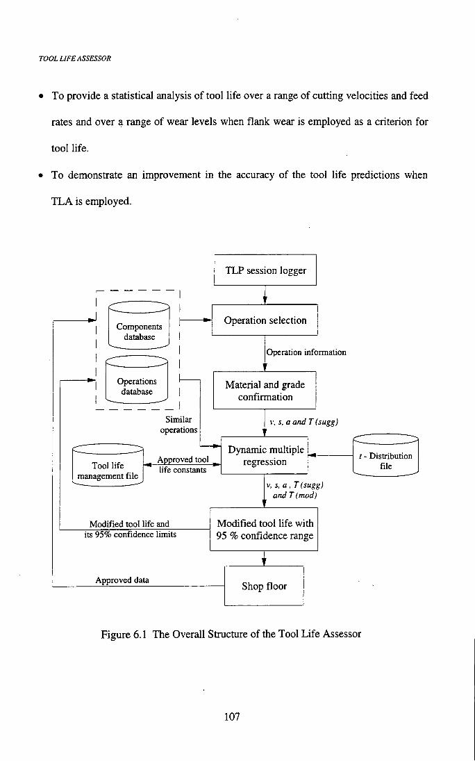
TOOL LIFE ASSESSOR
• To provide a statistical analysis of tool life over a range of cutting velocities and feed rates and over a range of wear levels when flank wear is employed as a criterion for tool life.
• To demonstrate an improvement in the accuracy of the tool life predictions when
TLA is employed.
Components database
Operations database
TLP session logger
Operation selection
Similar operations
Tool life management file
Operation information
Material and grade confirmation
Approved tool life constants
V, s, a and T(sugg)
Dynamic multiple regression
V, s, a, T(sugg) and T (mod)
Modified tool life and its 95% confidence limits
Approved data
Modified tool life with 95 % confidence range
Shop floor
t - Distribution file
Figure 6.1 The Overall Structure of the Tool Life Assessor
107

TOOL LIFE ASSESSOR
6.1 T L A FUNCTIONALITY
For any selected operation, either from the TLP session logger or from the operations
database, TLA retrieves all similar operations from the system's database based on the
following similarity criteria:
• Same carbide insert grade (TP 10, TP20 etc.)
• Same material sub-class (very soft steel, free cutting steel etc).
• Same type of cut (finishing, medium-roughing or roughing).
• Wet or dry cut.
If there is enough approved data (at least four points), TLA generates a dynamic
multiple regression to calculate the approved tool life coefficients (InC, -~ • and the
related degree of freedom ( d o . f ) .
do.f = n-p (6.1)
where; n is the number of the retrieved data and p is the number of parameters in the
model (InC, j; , j)-
Based on the calculated degree of freedom, the associated f-distribution critical value
will be retrieved from the f-distribution critical values database (Appendix 1) and the
95% confidence interval will be calculated.
Full job details and the modified tool life value (Tmod) with its 95% confidence interval
are displayed on the results screen and the user is asked to confirm whether they are
acceptable. If the user chooses "NO", the system will restart again showing the TLA top
108

TOOL UFE ASSESSOR
menu and will ask the user to select another operation. If "YES" option is selected, TLA gives the user choices for saving the operation and the modified tool life value with its 95% confidence interval in the approved database. TLA also saves the new calculated coefficients (/nC, > -p)^ the associated number of points, material sub-class, insert
grade and the type of cut in the management file (the structure of which will be
explained fully in the next Chapter).
The 95% confidence interval of tool life values from TLA shows a good degree of
confidence in approximating to the actual tool life values from the experiments. This
requires a maximum variance of the predicted true mean natural logarithmic-
A A
transformed tool life var [InT], where; the variance of the predicted InT^ at cutting
conditions x jg;
var [ Inn ] = xj [X^ X x , c (6.2)
T T where; x* and X is the transpose of the matrix x and X respectively. Generally, the
transpose ofnxp matrix isa.p xn matrix.
2 2
a is the variance of the InTi observations about the fitted line, a is usually estimated
with the residual variance S ^.
The method for calculating the variance will be shown in the next section.
109

TOOL UFE ASSESSOR
6.2 LEAST-SQUARES METHOD
The large variation of tool life data gives rise to a high degree of uncertainty in tool life
models and predicted tool life values. These levels of uncertainty make it difficult to
maintain the economic optimization of the manufacturing process. Therefore, large
numbers of tests are often performed to reduce this variation and this greatly increases
costs. For this reason statistical techniques such as transformation and least-squares
have been advocated to develop better mathematical methods to model and predict tool
life. In some experimental data, logarithmically transformed tool life showed increasing
variance for short tool lifetimes because of tough machining operations and cases in
which the tool life failure mechanism is changing. The lack of homogeneity of variance
over cutting conditions can be largely avoided by dividing the model data space into
three cutting types namely, finishing, medium roughing and roughing in which the least-
squares analysis can be employed with a high degree of certainty.
In multiple regression, several predictors are used to model a single response variable.
For each of the n cases observed, values for the response and for each of the predictors
are collected. If the response is called Y, and the predictors are called x7, X2, , \p (p
is the number of predictors), then the equation that expresses the response as a linear
function of the p predictors is estimated using the observed data. The model is
expressed by a linear equation:
Y=bo + b i X I + b 2 X 2 + +hpXp + £ (6.4)
When p = 2, equation 6.4 describes a two-dimensional plane in the three dimension {x\,
X2, Y) space (tool life model).
110

TOOL UFE ASSESSOR
When p = 2, equation 6.4 can be written as:
Y = bo-Hbi Xi-i-b2 X 2 + £ (6.5)
The logarithmic transformation of tool life equation is of the same form as equation 6.5.
A A ^ A
lnT = lnC + ( - j^ )lnv + ( - J )lns + £ (6.6)
where; In T is the random variable of the logarithmically transformed tool life, v is the
A A
cutting velocity, s is the feed rate, In C, and are parameters (to be estimated), and
e is the random error. Or, in matrix notation:
Y = Xe + e (6.7)
Let Y and e be « x 7 vectors whose elements are given by
Y =
InTj
lnT2
InT;
e=
Inej
lne2
Ine;
(6.8)
Also, define 0 to be the vector parameter of length 3x1, including the intercept InC,
e = InC _±
a _±
(6.9)
Define X to be « x 5 matrix given by:
X =
1 Invj Ins J
1 lnv2 Ins 2
1 Invi Insi
(6.10)
111

TOOL UFE ASSESSOR
The matrix X gives all of the observed values of the predictors, appended to the column of 7 's. The ith row corresponds to values for the ith case in the data; the columns of X correspond to the different predictors.
T
Matrices of the form X X met in regression work are always symmetric [Draper and
Smith 1981], that is to say that the element in the ith row and jth column is the same as
the element in the jth row and ith column. Thus, the transpose of a symmetric matrix is
the matrix itself Then the symmetric inverse is: n ^Invi ' A B C '
(X^ X)"^ = ^Invi ^Invi Ins I = B D E
^Insi ^ / n v j Ins I C E F
where;
B = - ^Invi ^[insif -Y,lnSi ^Inv^ /n^ j j / G
C = [j,lnvi Insi] - J^lnsi J,[lnvif] / G
D = !^nj^[lnsif - [J^lnsif^/G
E = - n ^[invjlnsj] - ^Invi ^Insi^ / G
F = \^nJXlnVif - [ X / n v , f } / G
and
112

TOOL UFE ASSESSOR
G = n XZ/nVj;^ "LllnSiP + 2 J^lnv^ J^lns^ SZnv- Zn - - n ['Zlnv^ Ins^P
Once we have estimated G (InC, . j ) from n observations of Y. However, in practice
one is generally interested in predicting the value /nT* of the random variable Y, at
given cutting conditions x = x , where;
InT* = X e + e (6.11)
where; x is any given cutting conditions
X =
1
Ins*
(6.12)
The variance can be calculated as follows:
var [lnn]= x i var e x (6.13)
where;
T r x ; = [1 Znv* Ins* (6.14)
(6.15)
By substituting equation 6.15 into equation 6.13, the result is equation 6.2.
The modified tool life value with 95% confidence intervals is given by:
InT* ± to.o25 ^var [InTJ + (6.16)
113

TOOL UFE ASSESSOR
Substituting equation 6.2 into equation 6.16
/n7; ± to.o25 X S Vl + X J [X^ X X , (6.17)
Where the degrees of freedom (d.o.f) for 0.025 are the same as the devisor in calculating
S ^ (see equation 6.3).
Equation 6.17 is used within the system to calculate the modified tool life value and its
95% confidence intervals for any given cutting conditions.
6.3 A N EXAMPLE
The cutting conditions and tool life values from the initial tool life tests when cutting
free-cutting steels (ENS) using TP20 insert grade under semi-roughing machining
conditions (Table 5.5 and Table 5.6) are logarithmically transformed to fi t the linear
model and are shown in Table 6.1.
Table 6.1 Cutting conditions and tool life values for TP20/EN8 Tapp min
V m/min
s mm/rev
In Tapp In V Ins
18.80 350 0.2 2.934 5.858 -1.609 21.32 330 0.2 3.06 5.799 -1.609 6.700 310 0.25 1.902 5.737 -1.386 13.13 295 0.28 2.575 5.687 -1.273
lnT=2.6lS lnv=5.11 lns=-\.Al
2](/nv,- - k ^ ) [inTi -M') = 0.068
2 {in Si - hTs) {in 7} - 1 ^ ) =-0.114
114

TOOL LIFE ASSESSOR
^{invi-lnvf = 0.0n
^[inSi-hTsf = 0.085
2{inVi - Jnv) [insi -lns)=- 0.0355
From multiple regression (equations 6.5 and 6.6):
A A
0.0681 = { ~ ) (0.0166) 0.0355)
A A
0.174 = { ~ ) (0.0355) (0.0847)
By solving equation (i) and equation (ii)
A
4 =3.2 A
and ^ = 2.74
(i)
(ii)
P
From equation 4.7
InC = 13.72
Equation (4.1) can be written as:
InT = 13.72 - 2.74 Inv - 3.2 Ins (iii)
Table 6.2, shows the tool life values (InT^nod) the associated residuals predicted by
the fitted model.
Table 6.2 The natural logarithmic tool life values and their residuals
InTapp InTmod Residuals e 2 e
2.934 3.125 -0.192 0.037 3.060 3.287 -0.227 0.052 1.902 2.744 -0.842 0.709 2.575 2.517 -0.058 0.003
115

TOOL UFE ASSESSOR
Equation 6.8, 6.9 and 6.10 can be defined as:
Y =
2.934 - 0.192 3.060
e = - 0.227
1.902 - 0.842 2.575 - 0.053
8 =
X =
1 5.858 -1.609 1 5.799 -1.609 1 5.737 -1.386 1 5.687 -1.273
xT = 1
5.858
13.72 -2.74 -3.2
1 1 5.799 5.737
1 5.6871
-1.609 -1.609 -1.386 -1.273
Also the matrix ( X ^ X) ^ can be defined as:
4 23.081 -5.877 -1 A B C ( X ^ x)-^ = 23.081 133.199 -33.947 = B E F
-5.877 -33.947 8.719 C F K
G =-7.759
A =-1.162
5 = 0.225
C = 0.093
D =-0.044
E=-0.018
F= 0.107
Then, for any given cutting conditions (x^) (say: v =340 and s = 0.2, the predicted value
A (InT) at this cutting conditions can be calculated from equation (iii) as follows:
A InT = 2.8973
Also we can define x* and x^
X * =
1.0 5.829
-1.609
xj=\l.0 5.829 -1.609
116

TOOL UFE ASSESSOR
np 7
We can calculate x* (X* X) x* as follows:
=1 1 5.829 -1.609
- 1.162 0.225 0.093 0.225 - 0.044 - 0.018 0.093 - 0.018 0.107
1.0 5.829
-1.609
= \0.0 -0.0025 - 0.184 1.0
5.829 -1.609
= 0.2814
The variance can be calculate as follows:
a = y e. , where n is the number of observations = 4. n-3 '
a2 = 0.800
Equation 6.2 can be written as:
varllnT* ] =0.284 x 0.8
The 95% confidence intervals can be calculated as follows:
InT = 2.8973± to.o25 x 0.894x -J 1 + 0.2814
The degree of freedom (d.o.f) = 4-3 = 1
From Appendix 7, and at 1 degree-of-freedom to.o25 = 12.7
InT =2.8973 ±12.7 x 0.894 x 1.1318
InT =2.8973 ± 12.84
117

Chapter 7
TOOL L I F E MANAGEMENT
In building a reliable tool life prediction system for a real factory which consists of
dozens of machines, hundreds of parts and thousands of cuts and operations every week,
it is very important to establish a method of collecting and processing feedback
information from cutting processes. In particular, methods were developed for
analyzing, continually or at fixed intervals, the variation in the tool life data calculated
by the two prediction modules (TLP and TLA) as well as the real approved results
collected from the shop floor in order to provide the necessary feed back information for
effective tool life control.
Tool life management (TLM), which is shown in Figure 7.1, has access to the approved
operations database and the management database file in order to retrieve the tool hfe
data suggested by the prediction and assessment modules (TLP and TLA) as well as the
approved tool life data collected from the shop floor. TLM studies the variations in
these retrieved data and provides feedback for the system, mainly TLA, in order to
adjust and improve future prediction results. TLM is a strategic, management tool
which can be used to assess the effectiveness and accuracy of tool life predictions over a
long period of time. It is designed to operate within an industrial environment and for
that, an appropriate interpretation of real tool life achieved is required. The
measurement of the wear land and the application of formal tool life criteria may be
118

TOOL UFE MANAGEMENT
unsustainable in most companies since they may involve extensive additional operations. Instead, the achieved, real tool life should be based on criteria presently applied by machinists such as change in chip size and shape, vibration and noise. The functions of TLM are described below.
Material, grade and type of cut selection
Management file
"Yes" if the variations is 5% or more
"Yes" if difference is getting bigger
"NO" if all the three checks results is NO
"Yes" if 5% or more is outside the limits
Check the variations between subsequent approved
tool life constants
NO" if the variations are less than 5%
Study the difference between the approved values (Japp) and the
modified values (Tmod) from TLA
'NO" if the difference is getting smaller
Check how many times Tapp lies within the 95% confidence
limits calculated by TLA
r
Components database
Operations database
Figure 7.1 The overall structure of the tool life management
7.1 TOOL LIFE MANAGEMENT FUNCTIONALITY
For any chosen material sub-class, insert grade and type of cut, the tool life management
module (TLM) retrieves tool life data from the matching operations available in the
operations database and the management file database based on the following similarity
criteria:
119
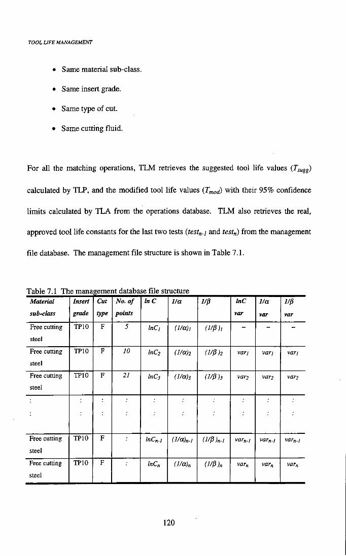
TOOL LIFE MANAGEMENT
• Same material sub-class.
• Same insert grade.
• Same type of cut.
• Same cutting fluid.
For all the matching operations, TLM retrieves the suggested tool life values iTsugg)
calculated by TLP, and the modified tool life values {Tmodl with their 95% confidence
limits calculated by TLA from the operations database. TLM also retrieves the real,
approved tool life constants for the last two tests {testn-i and test,^ from the management
file database. The management file structure is shown in Table 7.1.
Table 7.1 The management database file structure Material Insert Cut No. of InC lla 1/p InC I/a I / f i
sub-class grade type points var var var
Free cutting
steel
TPIO F 5 InCj (l/a)i
Free cutting
steel
TPIO F 10 lnC2 (l/a)2 (1/P)2 varj var I var]
Free cutting
steel
TPIO F 21 InCs (1/CC)3 (1/P)3 var2 var2 var2
Free cutting
steel
TPIO F InCn-i (l/a)n.i (I/P)n-J var„.j varn-i var„.i
Free cutting
steel
TPIO F InCn (l/ak (1/P)n var„ varn var„
120

TOOL UFE MANAGEMENT
For any selected combination of material sub-class, insert grade and type of cut, the tool life management (TLM) module has three main functions:
• Calculates the variations between the approved tool life constants in the last two
retrieved tests {testn-i and test,^.
• Calculates the difference between the approved tool life value {Tapp) collected from
the shop floor and the modified value (Tmod) predicted by TLA by using the approved
tool life constants in the last two retrieved tests.
• For all matching operations retrieved from the operations database, TLM counts how
many times (as a %) the approved tool life values lie within the 95% confidence
limits calculated by TLA.
7.1.1 The variation in approved tool life constants
For this check, T L M retrieves from the management database file the tool life data in
the last two approved records (testn-i and testn) and calculates the 5% values of the
variables lnC„.j, (17a )nj and (1/^ )„j where; n-1 is the observation before the last one.
T L M calculates the variations in the approved tool life constants calculated by multiple
regression in the last two tests as follows:
var (In C) = \ Zw C„ - In C„_; | (7.1)
var (17a) =1 ( 7 / « ) „ - ( 1 7 a ) „ . i \ (7.2)
var (1713 )= (17P - (1/P )n-i I (7-3)
121

TOOL UFE MANAGEMENT
Then TLM compares the variation for each constant, var (InC), var (17a) and var (17 P), with its 5% value in the (n-1) observation and the following conditions are checked:
• Condition 1: var (ZnC j <5 % of the Z«C„./value
• Condition 2: var (17a )<5%oi the (17a)„.] value
• Condition 3: var (i/jS) <5 % of the ( i/j3 value
If any of the above conditions is not true, TLM will automatically register a "YES"
option (i.e. there is a change in the new calculated constant(s) by more than 5% from the
previous calculated one). Otherwise, the "NO" option will be registered since there is
no significant change between the constant(s) calculated in testn.] and the tool life
constant(s) calculated in testn as a result of performing more tests. The user is allowed
to set any other limit in the variation allowed.
This function aims to record and study the variations in tool life constants calculated by
TLA as a result of adding more approved results. It is expected that initially there will
be wider variations in the tool life coefficients and subsequently these variations will be
reduced as a result of calculating the values by using more approved tests.
7.1.2 The difference between Tapp and Tmod
For the chosen material sub-class, insert grade and type of cut, TLM retrieves the
approved tool life values collected from the shop floor (Tapp) and the last two modified
122

TOOL LIFE MANAGEMENT
tool life values {Tmod) predicted by TLA. TLM calculates the difference between the
successive Tapp and Tmod sets and the following condition is checked:
• Condition 4: ^app ^mod < testn
^app ^mod testn-1
If the above test is true, TLM registers a "NO" option to indicate that the difference
between the approved and modified values in the last test {testn) is smaller than the
difference in the previous test (testn.i). Otherwise, a "YES" option is registered to
indicate that the difference is getting bigger. Of course, i f this happens it means that the
predictions have not reached a stable point and the particular set of approved results
cannot guarantee the accuracy of predictions.
7.1.3 The approved tool life and the boundary limits from T L A
For the given combination of material sub-class, insert grade, type of cut and cutting
fluid, TLM retrieves from the operations database the approved tool life values collected
from the shop floor and the modified tool life values with their 95% confidence
intervals as calculated by TLA. TLM counts how many times (%) the approved values
lie within the boundary limits calculated by TLA.
If 95% or more of the real tool life values lie within the boundary limits set by TLA,
TLM registers a "NO" option (i.e., the large majority of points are within the boundary
limits). Otherwise, a "YES" is registered (i.e., more than 5% of the approved tool life
values lie outside the boundary limits given by TLA). This check is very important
123

TOOL UFE MANAGEMENT
because it shows the accuracy of the system in predicting an interval for each modified tool life value, with 95% confidence that the approved value will be within this boundary.
Finally, TLM wil l consider that no changes have been registered if the results from the
previous three checks described in sections 7.1.1, 7.1.2 and 7.1.3 are "NO". This
indicates that the newly added approved points do not affect the prediction results and
the tool life constants (InC, , j ) calculated by TLA are considered to be stable. If
this is the case, TLM advises the user to stop recording any additional approved points
for the particular combination of material, grade and operation. The user is advised to
use the last calculated tool life constants for future predictions.
On the other hand, TLM considers that there were noticeable changes as a result of
collecting the last real data, i f any of the previous three checks results in "YES". This
means that the extra approved point improved the prediction results and the approved
tool life constants are not final. The user is advised to keep recording additional
approved points in order to improve further the predictions for the given combination.
The full detailed calculations of this analysis wil l be given in Chapter 8.
124
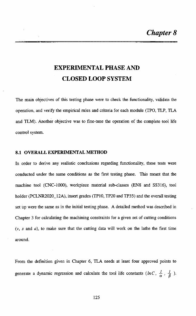
Chapter 8
EXPERIMENTAL PHASE AND
CLOSED LOOP SYSTEM
The main objectives of this testing phase were to check the functionality, validate the
operation, and verify the empirical rules and criteria for each module (TPO, TLP, TLA
and TLM). Another objective was to fine-tune the operation of the complete tool life
control system.
8.1 O V E R A L L E X P E R I M E N T A L METHOD
In order to derive any realistic conclusions regarding functionality, these tests were
conducted under the same conditions as the first testing phase. This meant that, the
machine tool (CNC-1000), workpiece material sub-classes (ENS and SS316), tool
holder (PCLNR2020_12A), insert grades (TPIO, TP20 and TP35) and the overall testing
set iip were the same as in the initial testing phase. A detailed method was described in
Chapter 3 for calculating the machining constraints for a given set of cutting conditions
(v, s and a), to make sure that the cutting data will work on the lathe the first time
around.
From the definition given in Chapter 6, TLA needs at least four approved points to
generate a dynamic regression and calculate the tool life constants (InC, , ).
125
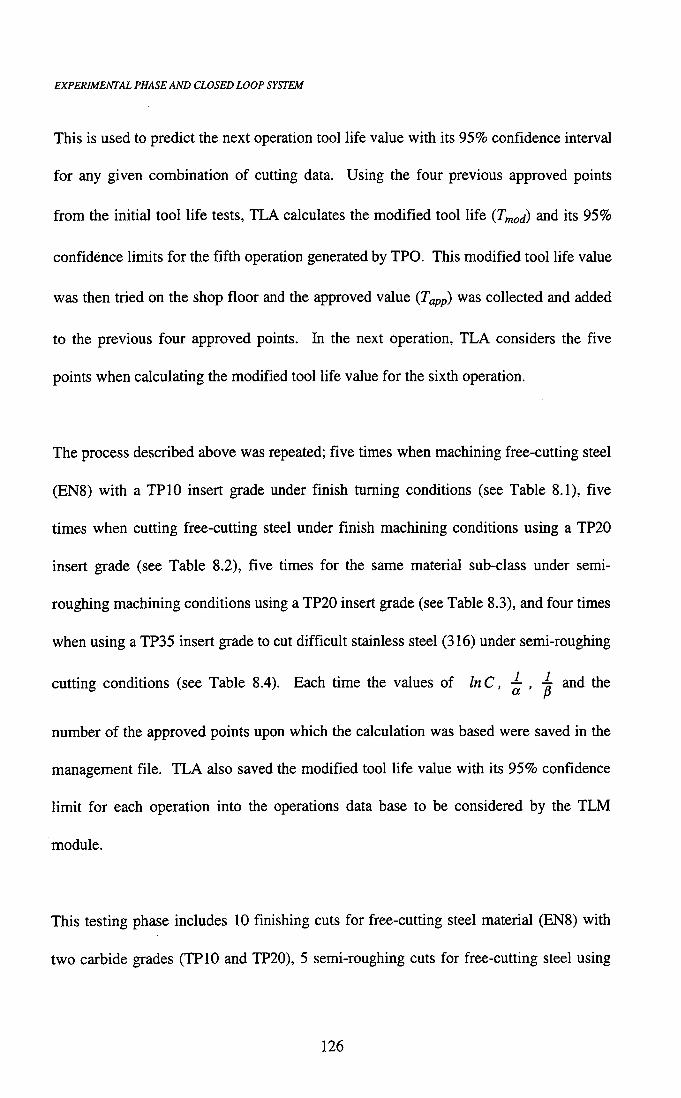
EXPERIMENTAL PHASE AND CLOSED LOOP SYSTEM
This is used to predict the next operation tool life value with its 95% confidence interval for any given combination of cutting data. Using the four previous approved points from the initial tool life tests, TLA calculates the modified tool life (Tnod) and its 95% confidence limits for the f if th operation generated by TPO. This modified tool life value was then tried on the shop floor and the approved value (Tapp) was collected and added
to the previous four approved points. In the next operation, TLA considers the five
points when calculating the modified tool life value for the sixth operation.
The process described above was repeated; five times when machining free-cutting steel
(EN8) with a TPIO insert grade under finish tuming conditions (see Table 8.1), five
times when cutting free-cutting steel under finish machining conditions using a TP20
insert grade (see Table 8.2), five times for the same material sub-class under semi-
roughing machining conditions using a TP20 insert grade (see Table 8.3), and four times
when using a TP35 insert grade to cut difficult stainless steel (316) under semi-roughing
cutting conditions (see Table 8.4). Each time the values of InC, , and the
number of the approved points upon which the calculation was based were saved in the
management file. TLA also saved the modified tool life value with its 95% confidence
limit for each operation into the operations data base to be considered by the TLM
module.
This testing phase includes 10 finishing cuts for free-cutting steel material (EN8) with
two carbide grades (TPIO and TP20), 5 semi-roughing cuts for free-cutting steel using
126

EXPERIMENTAL PHASE AND CLOSED LOOP SYSTEM
TP20 insert grade and 5 semi-roughing cuts for difficult stainless steel material (316) using TP35 carbide grades.
8.1.1 Results from machining free cutting (ENS) steel with TPIO insert grade
This set of tool life observations was obtained by cutting free cutting steel (ENS) with
TPIO insert grade under finish-machining conditions. The initial cutting conditions
used in this set were calculated by TPO module and are shown in Table S.l. The
suggested tool life values (^j^^^) calculated by TLP using the theoretical constants, and
the modified tool life values (Tmod) predicted by TLA using the approved constants are
also shown in Table S.l. Table S.l shows that the modified values for tests 2 and 5 are
considerably different from the approved values. This can be attributed to the stochastic
nature of tool life and to the fact that those predictions were based on a limited number
of approved points. The predictions will be improved when more approved data
becomes available. On the other hand, the other three tests showed a good correlation
between predictions and approved values.
The surface roughness (Ra) for these tests varied between 1.2 to 2.3 pm in order to keep
the surface roughness within limits normally associated with finishing cuts.
127

EXPERIMENTAL PHASE AND CLOSED LOOP SYSTEM
Machine Tool CNC-1000 Tool Holder PCLNR2020 12A Insert Type CNMG120408 MF2 Insert Grade TPIO Workpiece Dimension Length=200mm and Diameter=100 mm Cutting Fluid Rocol-Ultracut 370
Test No. Test I Test 2 Tests Test 4 Tests Cutting Depth (mm) 1.5 0.5 1.4 0.8 1.5
Parameters Feed (mm/rev) 0.18 0.24 0.17 0.22 0.18
Velocity (m/min) 450 490 405 410 430
Tsugg (min) 8.99 5.59 14.82 12.98 11.07
Tool Life Tmod (min) 8.69 4.61 13.77 12.02 11.14
Tapp (min) 8.0 8.4 12.02 13.07 8.52
Surface Roug. ^a(|im) 1.3 2.3 1.2 1.9 1.3
Figure 8.1 shows the tool flank wear measurements with machining time for this series
of tests. The average flank wear on the cutting edge is almost 0.05 mm after about 3
min of cutting in all these tests. Picmres of some inserts employed in this set of tests are
shown in Appendix 6A.
0.4
0.3
? I 0.2
c a •^0.1
Test 4
Tests ,
Test 2 / / Tets5
H—
2 4 6 8 10
Machining time (min) 12 14
Figure 8.1. Flank wear versus machining time for finishing EN8 with TPIO
128

EXPERIMENTAL PHASE AND CLOSED LOOP SYSTEM
I
Figure 8.2 shows the comparison of the three tool l i fe values (Tsugg , T^od and Tapp) for
the above five observations. In test 1 and 3 it is clear that the modified tool l i fe is
getting closer to what actually achieved in the experiment. In test 5 the two predicted
values are very close together and the actual tool l ife was slightly smaller. The
hypothesis that a modification of tool l i fe w i l l bring it closer to the experimental value is
not directly proven by tests 2 and 4. Variation in set-up conditions, vibration and the
randomness of tool l i fe are the main reasons for this behaviour and it is expected that
additional real values w i l l improve future predictions.
16 -
14 -
12 -
10 •
life
8 •
Tool
6 -
4 -
2 -
0 -
• T(sugg) El T (mod)
T(app)
Test number
Figure 8.2 Tool l i fe values for f ive TPIO inserts when finishing ENS
Figure 8.3, shows the approved tool l i fe values and the 95% boundary limits of the Tmod
values predicted by T L A . It can be seen that the approved tool l ife values in tests 2, 3,4
and 5 were outside the confidence limits calculated by T L A . For test 2, the predicted
limits were based on just 5 approved points. In test 3, the predicted modified value was
129

EXPERIMENTAL PHASE AND CLOSED LOOP SYSTEM
based on 6 approved points and the lower l imit predicted by T L A is higher than the Tapp by approximately 1 min. In test 5, the modified value was based on 8 approved points and the lower l imi t is higher than Tapp by approximately 2 min. However, the modified values for these tests were much closer to the approved values than the suggested values calculated by TLP based on theoretical tool l i fe constants. These results show that the 95% confidence l imit is not met in most cases using this set of approved data. Clearly, additional tests are needed to satisfy this tight confidence limit. However, test 3 and 4 would have satisfied a less light confidence limit.
14
. | 10 -1-
r
^ TLA limits
• T(app)
Test Number
Figure 8.3 Real tool l ife values and boundary limits calculated by T L A
8.1.2 Results from machining free cutting steel (ENS) with TP20 msert grade
The second and third sets of 5 experiments correspond to cutting EN8 steel with a TP20
insert grade under finish and medium-roughing machining conditions respectively.
130

EXPERIMENTAL PHASE AND CLOSED LOOP SYSTEM
Table 8.2 shows the theoretical cutting conditions calculated by TPO and employed for f ive tests when finish machining EN8 free cutting steel with a TP20 insert grade. The tool l ife value calculated by TLP iJsugg) and the modified value {Tf^od) predicted by T L A for each set of cutting condition are also shown in Table 8.2. It is obvious that the T L A predictions were very close to the real values collected f rom the shop floor. The surface finish varied between 1.2 to 2.3 j im.
Table 8.2 Finish machining conditions of EN8 free-cutting steel with TP20 grade
Machine Tool CNC-1000 Tool Holder PCLNR2020_12A Insert Type CNMG120408_MF2 Insert Grade TP20 Workpiece Dimension Length=200mm and Diameter=100 mm Cutting Fluid Rocol-Ultracut 370
Test No. Testl Test 2 Tests Test 4 Tests Cutting Depth (mm) 0.50 1.20 1.40 0.90 0.80
Parameters Feed (mm/rev) 0.24 0.18 0.17 0.21 0.22
Velocity (m/min) 470 380 360 410 430
Tsugg (min) 3.04 8.82 11.50 5.94 4.70
Tool L i fe Tmod (mm) 3.04 10.87 13.13 7.31 6.15
Tam (min) 4.90 10.05 13.07 8.58 6.47
Surface Roug. Ra (fim) 2.3 1.3 1.2 1.8 1.9
The wear rates versus machining time for the five TP20 inserts of this series of tests are
plotted in Figure 8.4. It can be observed that the TP20 inserts exhibit a wide range of
wear patterns when cutting ENS free-cutting steel at this range of cutting conditions.
Pictures of some TP20 inserts used in theses tests are shown in Appendix 6B.
131

EXPERIMENTAL PHASE AND CLOSED LOOP SYSTEM
0.4 T
0.3 + £ E
go.2
c CO
0.1
0.0
Testl Tests Test 2
// Test4 , - y Test 3
6 8 10 Cutting time (min)
12 14
Figure 8.4 Flank wear versus machining time when finishing ENS with TP20
Figure 8.5 shows the system's tool l ife predictions and the real observed values when
finishing ENS using the TP20 insert grade. It is obvious that the modified values were
much closer to the real values than the original values calculated by TLP in test 2, 3, 4
and 5. Clearly, for this series of tests the modification of tool l ife (Tmod) brought the
initial prediction (Tsugg) closer to what is actually achieved (Tapp). These results prove
the essential hypothesis of using approved data to modify theoretical tool l ife
predictions.
132
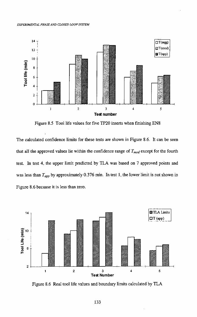
EXPERIMENTAL PHASE AND CLOSED LOOP SYSTEM
14 J 12 --
10 -•
1 8 -•
0)
6 -•
o o 1- 4 -•
2 -•
0 --
• T(sugg)
ElT(mod)
HT(app)
Test number
Figure 8.5 Tool l i fe values for f ive TP20 inserts when finishing ENS
The calculated confidence limits for these tests are shown in Figure 8.6. It can be seen
that all the approved values lie within the confidence range of T^od except for the fourth
test. In test 4, the upper l imit predicted by T L A was based on 7 approved points and
was less than Tapp by approximately 0.376 min. In test 1, the lower l imit is not shown in
Figure S.6 because it is less than zero.
14
= 10 E
r
^ TLA limits
• T(app)
Test Number
Figure 8.6 Real tool l ife values and boundary limits calculated by T L A
133

EXPERIMENTAL PHASE AND CLOSED LOOP SYSTEM
Table 8.3 shows the calculated cutting conditions and the predicted tool l i fe values for f ive observations when machining ENS free-cutting steel using TP20 carbide grade under medium-roughing machining conditions. The machine power is approximately 5 k W for all tests and this is close to the maximum power of the lathe for prolonged operation.
It can clearly be seen that the initial tool l i fe predictions (Tsugg) are considerably higher
than the real values {Tapp). The theoretical tool l i fe constants would result in
unexpected, premature tool failure with catastrophic consequences. On the other hand
the tool l i fe constants calculated by using approved data is giving results {Tmod) which
are very close to the obtained values in tests 1,4, and 5.
Table 8.3 Semi-roughing machining conditions of ENS steel with TP20 grade
Machine Tool CNC-1000 Tool Holder PCLNR2020_12A Insert Type CNMG120408_MF3 Insert Grade TP20 Workpiece Dimension Length=200mm and Diameter=100 mm Cutting Fluid Rocol-Ultracut 370
Test No. Testl Testl Tests Test 4 Tests Cutting Depth (mm) 2.0 1.9 1.7 1.6 1.8
Parameters Feed (mm/rev) 0.2 0.23 0.26 0.27 0.24
Velocity (m/min) 340 320 305 300 315
TsuRg (min) 29.0 26.55 24.01 23.46 25.53
Tool L i f e Tmod (min) 18.26 13.93 9.45 9.18 11.74
Tapp (min) 19.45 7.8 11.17 9.13 11.05
Mach. Power /'(kW) 5.53 5.5 5.123 4.75 5.17
Spindle Speed rpm (rev/min) 1804.67 1643.72 1471.72 1405.02 1567.48
134

EXPERIMENTAL PHASE AND CLOSED LOOP SYSTEM
Figure S.7 shows the wear measurements along the flank face of the tool as a function of machining time for this set of experiments. Again, pictures of some inserts used in this set of tests are shown in Appendix 6C.
0.4 T
0.3 + E E
^ 0.2 + I C
n 0.1
0.0
Test 4 X
Tests / Testl
Test:
/ / . 7
Tests
H 1 -
6 8 10 12 14 16 18 20
Cutting time (min)
Figure 8.7 Flank wear versus machining time when semi-roughing ENS with TP20
Figure 8.8 shows the improvements in the system's predictions when the modified
values iJmod) from T L A are considered. For all tests the modified values are closer to
the real approved values than the initial ones as discussed above. This set of tests
validates the use of real data in a closed-loop tool l i fe prediction system.
135

EXPERIMENTAL PHASE AND CLOSED LOOP SYSTEM
30 T
25
C 20
« 15
O O 10
• T(sugg) ITCinod)
Test number
Figure 8.8 Tool l i fe values for five TP20 inserts when semi-roughing ENS
Figure 8.9 shows the approved tool l i fe {Tapp) values and the boundary limits of Tnod
calculated by T L A . I t is clear that the approved values lie within dlie T L A boundary
ranges in tests 1,4 and 5. Test 3 is a marginal failure and test 2 is a failure.
30
25
20 +
15 o o
10
^ T L A Limits
• T(app)
Test Number
Figure 8.9 Real tool l ife values and boundary limits calculated by T L A
136

EXPERIMENTAL PHASE AND CLOSED LOOP SYSTEM
8.1.3 Results from machining difficult stainless steel 316 with TP35 insert grade
A I S I 316 austenitic stainless steel is a difficult material to machine. Even when using
low cutting velocity, BUE formation occurs and severe adhesive wear is readily initiated
[Soderberg 1981; Soderberg 1983]. In addition, segmented chip formation occurs
readily and edge chipping is often a great problem [Soderberg 1981].
Table 8.4, shows the medium-roughing machining conditions calculated by TPO and
employed for 4 observations to cut difficult to machine stainless steel material (SS316)
with a TP35 insert grade. The tool life values suggested by the system (Tsugg and T^od)
and the approved values (Tapp) are also shown in Table 8.4.
The calculated power values were close to the maximum 7.5 kW, for a 30-minute
operation of the lathe used. The cutting velocities employed for these tests are within
the range of tool manufacturer's recommendations and result in low spindle speeds.
Table 8.4 shows that the tool l i fe predictions using catalogue data (Tsug^ result in a
serious underestimation of tool l ife. The approved results create a completely different
regression curve using T L A , which modifies the suggested tool l i fe to get closer to
results obtained f rom the tests. These tests also validate the hypotheses that theoretical
calculations may be widely inaccurate and that use of dynamic regression can improve
the accuracy of tool l i fe prediction.
137

EXPERIMENTAL PHASE AND CLOSED LOOP SYSTEM
Table 8.4 Semi-roughing conditions of SS316 stainless steel with TP35 grade Machine Tool CNC-1000 Tool Holder PCLNR2020_12A Insert Type CNMG120404_MF3 Insert Grade TP35 Workpiece Dimension Length=200 mm and Diameter=75 mm Cutting Fluid Rocol-Ultracut 370
Test No. Testl Test 2 Tests Test 4 Cutting Depth (mm) 3.0 3.0 3.0 3.0
Parameters Feed (mm/rev) 0.3 0.25 0.4 0.3
Velocity (m/min) 140 120 100 135
Tsugg (min) 1.24 2.40 5.29 1.45
Tool L i f e Tmod (min) 8.09 23.43 8.82 8.22
Tapp (min) 6.30 23.70 8.45 8.32
Mach. Power 7.12 5.472 6.4 6.87
Spindle Speed rpm (rev/min) 990.79 849.25 707.7 955.4
Figure 8.10 shows the growth of the width of the flank wear as a function of machining
time for the group of TP35 inserts. These results confirm the characteristics of the flank
wear wi th machining time shown in the initial testing phase (see Figure 5.8). Pictures of
some inserts employed in this set of tests are shown in Appendix 6D.
0.4
^0.3 E
S 0.2
I 0.1
0.0
Test 4 Testl
/ ^ Test 3
Test 2
10 15
Cutting time (min) 20 25
Figure 8.10 Flank wear versus machining time when semi-roughing SS316 with TP35
138
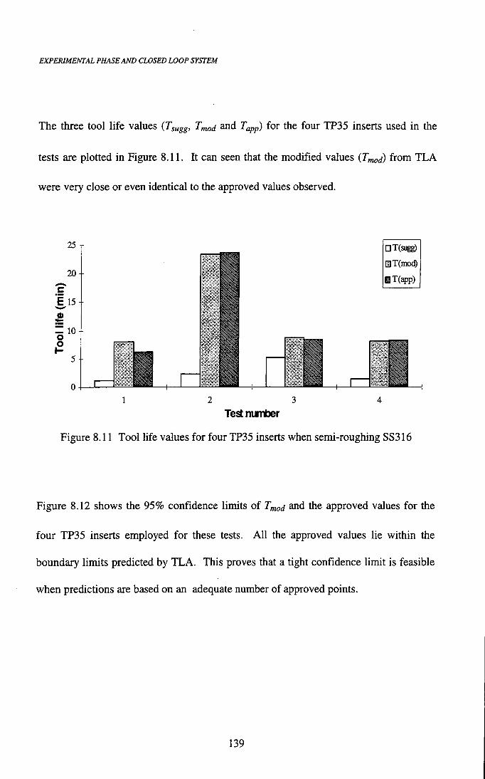
EXPERIMENTAL PHASE AND CLOSED LOOP SYSTEM
The three tool l i fe values (Tsugg, T^od and Tapp) for the four TP35 inserts used in the
tests are plotted in Figure 8.11. It can seen that the modified values (T^od) from T L A
were very close or even identical to the approved values observed.
25
20 +
I 15 4
= 10 +
5
• T ( s i ^
ll]T(mod)
ST(app)
1 4 2 3
Test number
Figure 8.11 Tool l ife values for four TP35 inserts when semi-roughing SS316
Figure 8.12 shows the 95% confidence limits of Tmod and the approved values for the
four TP35 inserts employed for these tests. A l l the approved values lie within the
boundary limits predicted by T L A . This proves that a tight confidence limit is feasible
when predictions are based on an adequate number of approved points.
139

EXPERIMENTAL PHASE AND CLOSED LOOP SYSTEM
25 J
20 --
••J 10 o
5 +
^ T L A limits
• T(app)
2 3 Test Number
Figure 8.12 Real tool l i fe values and boundary limits calculated by T L A
8.2 RESULTS FROM TESTING TLM
As discussed in Chapter 7, for any selected combination of material sub-class, insert
grade and type of cut, T L M has three main functions:
• Study the variations in the approved tool l ife constants (InC, , ) when new
approved data becomes available.
• Study the difference between the approved tool l i fe values (Tapp) and the modified
values (Tmod) predicted by T L A .
• Study how many times the approved values (Tapp) lie within the 95% confidence
limits calculated by T L A .
140

EXPERIMENTAL PHASE AND CLOSED LOOP SYSTEM
8.2.1 TLM results when finishing ENS free cutting steel using TPIO insert grade • Variations in tool life constants
T L M retrieves f rom the management file the last two sets of the approved tool l ife
constants {InCn-i, )„.; , ( j )n-i ) and ( /«C„ , j„ . ( j )n) calculated by
T L A as shown in Table 8.5.
Table 8.5 Management f i le when finish machining ENS using TPIO insert grade Material sub-class
Insert grade
A o. of points
Cut type
InC 1/a 1 / p InC var ( I / a ) var
( 1 / p ) var
free-cutting steel
TPIO 7 F 19.001 2.801 0.223
free-cutting steel
TPIO 8 F 19.891 2.935 0.184 0.8896 0.1335 0.0394
For the lnC„_j, (— and (-jz ) „ _ ; , T L M calculates the 5% values which are
0.95005, 0.14005, and 0.01127 respectively. T L M calculates the variations in the
approved constants between {n-1) and (n) set as shown in Table 8.5.
T L M compares the absolute values of the variations in the approved tool l i fe constants
wi th their 5% value. I f a variation is larger than the 5% value, a noticeable change of
constants is registered (the result of this test is YES). This is the case herein since the
variation in ( 7 / p ) value is greater than its 5% value (i.e., 0.0394 > 0.01127).
141
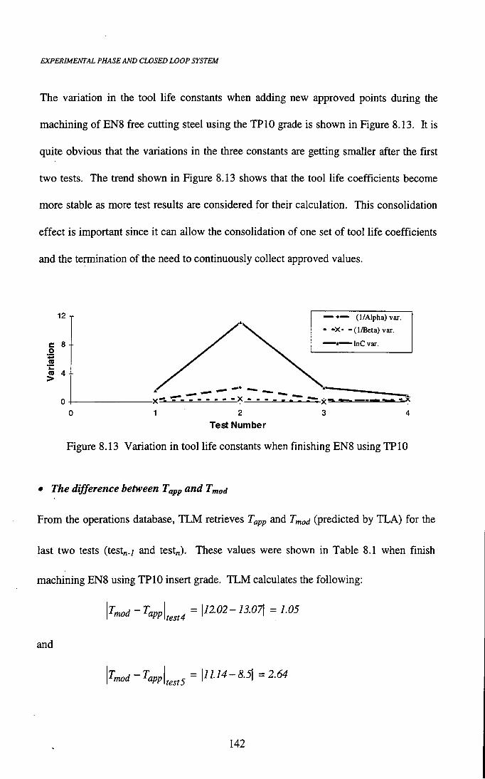
EXPERIMENTAL PHASE AND CLOSED LOOP SYSTEM
The variation in the tool l i fe constants when adding new approved points during the machining of ENS free cutting steel using the TPIO grade is shown in Figure 8.13. It is quite obvious that the variations in the three constants are getting smaller after the first two tests. The trend shown in Figure 8.13 shows that the tool l i fe coefficients become more stable as more test results are considered for their calculation. This consolidation effect is important since it can allow the consolidation of one set of tool l ife coefficients and the termination of the need to continuously collect approved values.
12
c 8 o
« 4 +
— (1/AIpha) var.
I - - X - -(1/Beta) var.
InC var.
Test Number
Figure 8.13 Variation in tool l i fe constants when finishing ENS using TPIO
• The difference between Tapp and Tmod
From the operations database, T L M retrieves Tapp and Tmod (predicted by T L A ) for the
last two tests (test„.7 and test„). These values were shown in Table 8.1 when finish
machining ENS using TPIO insert grade. T L M calculates the following:
"^mod app test4 = \12.02-13.07\ = 1.05
and
'^mod ^app tests = \lU4-8.5\ =2.64
142

EXPERIMENTAL PHASE AND CLOSED LOOP SYSTEM
T L M checks i f
^mod ^app testn ^mod ^app testn-1
This condition means that the modified value predicted by T L A in the last test is closer
to its observed value than in the previous test. In this example, this condition is not true
{2.64 > 1.05) and the fact that there is no reduction in the variation is registered (again
the result of this check is YES).
• Tapp and the boundary limits calculated by TLA
When finish machining ENS using the TPIO insert grade, T L M retrieves the approved
tool l i fe values and the boundary limits of T^od predicted by T L A from the operations
database. Table 8.6 shows these values.
Table 8.6 Tapp and T^od with its 95 % confidence limits Test no. Tapp Tmod + limits In Out
1 8.00 8.69 ±3.295 X
2 8.40 4.61 + 1.189 X
3 12.02 13.77 ±0 .704 X
4 13.07 12.02 + 0.674 X
5 8.52 11.14 + 0.466 X
T L M checks how many times the approved tool l i fe value collected from the shop floor
lies within the boundary limits calculated by T L A as shown in Figure 8.3 and Table 8.6.
I f 95% or more lie within the boundary limits it is considered that the real values are
effectively within the confidence limits. Otherwise, the fact that there is a violation of
143
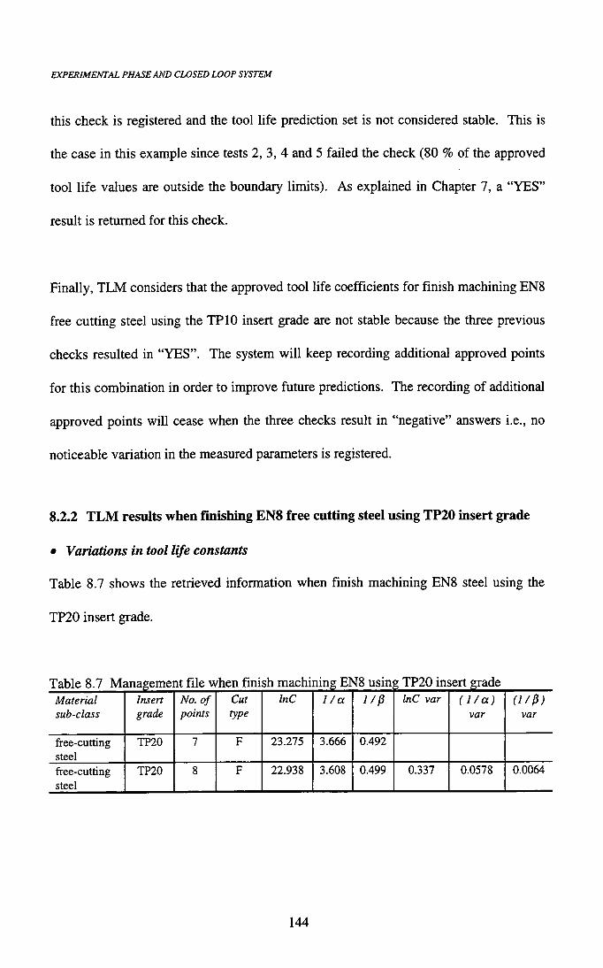
EXPERIMENTAL PHASE AND CLOSED LOOP SYSTEM
this check is registered and the tool l i fe prediction set is not considered stable. This is the case in this example since tests 2, 3, 4 and 5 failed the check (SO % of the approved tool l i fe values are outside the boundary limits). As explained in Chapter 7, a "YES" result is returned for this check.
Finally, T L M considers that the approved tool l i fe coefficients for finish machining ENS
free cutting steel using the TPIO insert grade are not stable because the three previous
checks resulted in "YES". The system w i l l keep recording additional approved points
for this combination in order to improve future predictions. The recording of additional
approved points w i l l cease when the three checks result in "negative" answers i.e., no
noticeable variation in the measured parameters is registered.
8.2.2 TLM results when fmishing EN8 free cutting steel using TP20 insert grade
• Variations in tool life constants
Table 8.7 shows the retrieved information when finish machining ENS steel using the
TP20 insert grade.
Table 8.7 Management f i le when finish machining ENS using TP20 insert grade Material sub-class
Insert grade
No. of points
Cut type
InC 1/a 1/P InC var (1/a) var var
free-cutting steel
TP20 1 F 23.275 3.666 0.492
free-cutting steel
TP20 8 F 22.938 3.608 0.499 0.337 0.0578 0.0064
144
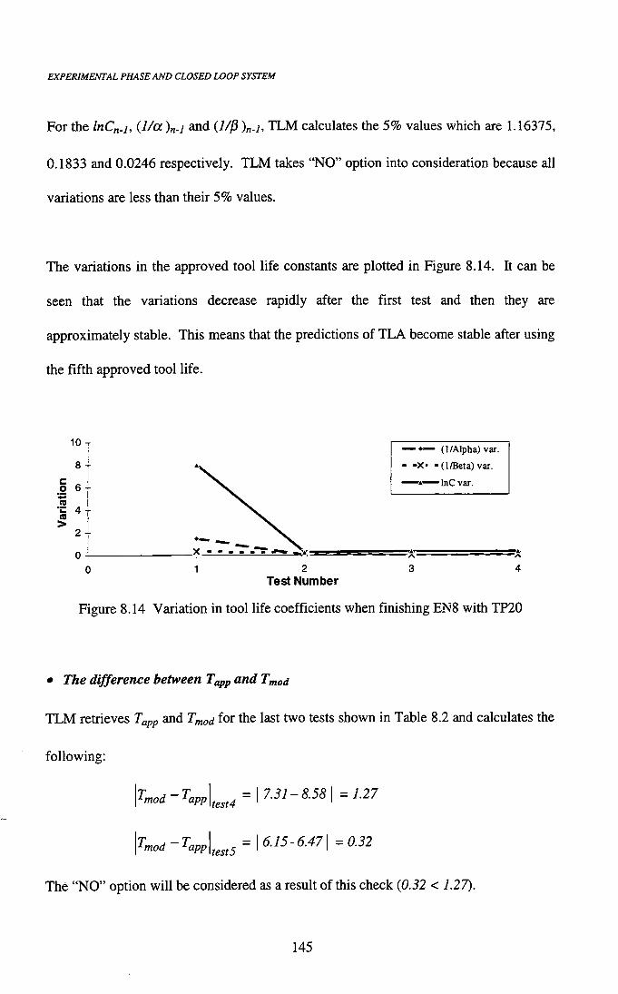
EXPERMENTAL PHASE AND CLOSED LOOP SYSTEM
For the /nC„.;, (1/a )„.; and (l/p )„.;, T L M calculates the 5% values which are 1.16375, 0.1833 and 0.0246 respectively. T L M takes "NO" option into consideration because all variations are less than their 5% values.
The variations in the approved tool l ife constants are plotted in Figure 8.14. It can be
seen that the variations decrease rapidly after the first test and then they are
approximately stable. This means that the predictions of T L A become stable after using
the f i f t h approved tool l i fe .
10 J
8 -•
I 6 n CO >
2 -•
— — (1/Alpha) var.
- - X - -(1/Beta) var.
Test Number
Figure 8.14 Variation in tool l i fe coefficients when finishing ENS with TP20
• The difference between Tapp and Tmod
T L M retrieves Tapp and Tmod for the last two tests shown in Table 8.2 and calculates the
fol lowing:
T^mod '^app
test4 = I 7.57-S.5SI =1.27
tests = \6.15-6.47\ =0.32
The "NO" option w i l l be considered as a result of this check {0.32 < 1.27).
145

EXPERIMENTAL PHASE AND CLOSED LOOP SYSTEM
• Tapp and the boundary limits calculated by TLA
The Tapp and the T,nod values with its 95% confidence limits retrieved by T L M for this
set of tests are shown in Table 8.8.
Table 8.8 Tgpp and Tmod with its 95 % confidence limits Test no. T ± limits In Out
1 4.90 3.04 ±9.264 X
2 10.05 10.87 ± 1.606 X
3 13.07 13.13 + 0.975 X
4 8.58 7.31 ± 0.737 X
5 6.47 6.15 ± 0.634 X
T L M calculates how many times the approved tool l ife values lie within the boundary
limits calculated by T L A as shown in Figure 8.6 and Table 8.8. T L M takes "YES" (the
approved tool l i fe showed an unacceptable f i t with regard to the confidence limits)
option because test 4 is outside the boundary limits (20% outside the limits).
Finally, T L M considers "YES" option for this combination (material, grade and type of
cut) because the last check results in "YES". The "YES" option indicates that the
approved tool l i fe coefficients are not stable and i t is recommended to keep recording
additional approved points. It must be noted that in this case the failure is marginal and
a wider confidence l imit would have resulted in stable coefficients.
146

EXPERIMENTAL PHASE AND CLOSED LOOP SYSTEM
8.2.3 TLM results when machining ENS free cutting steel using TP20 insert grade
under semi-roughing conditions
• Variations in tool life constants
Table 8.9 shows the required information retrieved by T L M from the management file
to apply this check.
Table 8.9 Management file when semi-roughing EN8 using Material sub-class
Insert grade
No. of points
Cut type
InC 1/a InC var ( 1 / a ) var
(1/^) var
free-cutting steel
TP20 1 MR 10.202 2.028 2.956
free-cutting steel
TP20 8 MR 10.200 2.079 2.962 0.002 0.051 0.006
'P20 insert grade
As in the previous two sets of tests, the 5% values of InCn-i, {l/oc )n-i and ( i / ^ )„.;
calculated by T L M are 0.51, 0.104 and 0.1478 respectively. This check is successful
and T L M registers the " N O " option since all the variations are less than their 5 %
values. Figure 8.15 shows the variation in the approved tool l i fe coefficients for these
tests.
4
3
c 1 = 1 1
— • — (l/Alpha) var.
- - X - - (1/Beta) var.
b C var.
Test Number
Figure 8.15 Variation in tool l ife coefficients when semi-roughing ENS with TP20
147

EXPERIMENTAL PHASE AND CLOSED LOOP SYSTEM
Figure 8.15 shows that the coefficients become stable after the second test and their
variation is negligible in subsequent tests. This means that different modified values
would have been calculated for the first two tests shown in Figure 8.8.
• The difference between Tapp and Tmod
T L M calculates the difference between the approved tool l i fe values and the modified
tool l i fe values for the last two tests shown in Table 8.3.
T,n^-T^pl,„=0.05
In this case, T L M registers a "YES" option because the difference is getting bigger.
• Tapp and the boundary limits calculated by TLA
For semi-roughing EN8 steel using TP20 insert grade, T L M retrieves the values shown
in Table 8.10 f rom the operations database.
Table 8.10 Tgpp and Tmod with its 95 % confidence limits Test no. T Tmod ± limits In Out
1 19.45 18.26 ± 10.241 X
2 7.80 13.93 ± 2.021 X
3 11.17 9.48 ± 1.558 X
4 9.13 9.18 ± 1.193 X
5 11.60 11.36 ±1.115 X
148
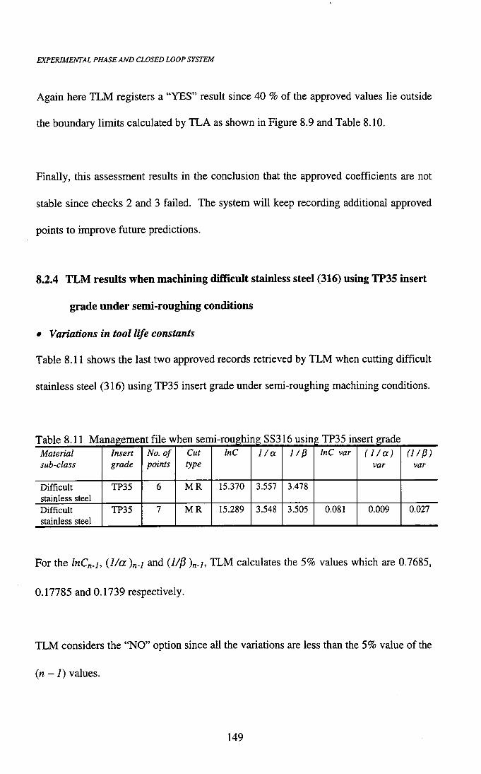
EXPERIMENTAL PHASE AND CLOSED LOOP SYSTEM
Again here T L M registers a "YES" result since 40 % of the approved values lie outside the boundary limits calculated by T L A as shown in Figure 8.9 and Table 8.10.
Finally, this assessment results in the conclusion that the approved coefficients are not
stable since checks 2 and 3 failed. The system w i l l keep recording additional approved
points to improve future predictions.
8.2.4 TLM results when machining difficult stainless steel (316) using TP35 insert
grade under semi-roughing conditions
• Variations in tool life constants
Table 8.11 shows the last two approved records retrieved by T L M when cutting difficult
stainless steel (316) using TP35 insert grade under semi-roughing machining conditions.
Table 8.11 Management f i le when semi-roughing SS316 usin g TP35 insert grade Material sub-class
Insert grade
No. of points
Cut type
InC 1/a I / p InC var ( 1 / a ) var var
Difficult stainless steel
TP35 6 MR 15.370 3.557 3.478
Difficult stainless steel
TP35 7 MR 15.289 3.548 3.505 0.081 0.009 0.027
For the InCn-i, )n-l and (1/p )„.;, T L M calculates the 5% values which are 0.7685,
0.17785 and 0.1739 respectively.
T L M considers the "NO" option since all the variations are less than the 5% value of the
(n - 7) values.
149
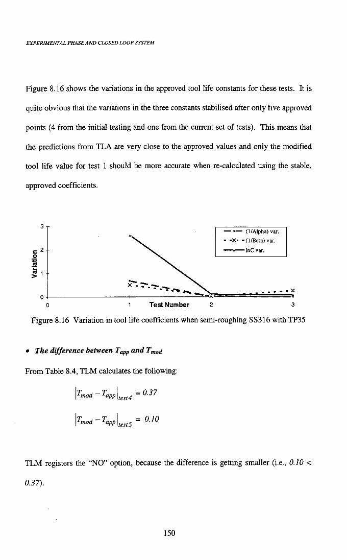
EXPERIMENTAL PHASE AND CLOSED LOOP SYSTEM
Figure 8.16 shows the variations in the approved tool l ife constants for these tests. It is
quite obvious that the variations in the three constants stabilised after only five approved
points (4 f rom the initial testing and one from the current set of tests). This means that
the predictions f rom T L A are very close to the approved values and only the modified
tool l i fe value for test 1 should be more accurate when re-calculated using the stable,
approved coefficients.
• • — (1/Alpha) var.
- X - -(1/Beta) var.
InC var.
0 1 Test Number 2 3
Figure 8.16 Variation in tool l i fe coefficients when semi-roughing SS316 with TP35
• The difference between Tapp and Tmod
From Table 8.4, T L M calculates the following:
^mod '^app
^mod ^app
test4 = 0.37
tests = 0.10
T L M registers the "NO" option, because the difference is getting smaller (i.e., 0.10 <
0.37).
150

EXPERIMENTAL PHASE AND CLOSED LOOP SYSTEM
• Tapp and the boundary limits calculated by TLA
The retrieved information for this check is shown in Table 8.12.
Table 8.12 Tg^,, and T„iod with its 95 % confidence limits Test no. Tapp Tmod ± limits In Out
1 6.30 8.09 ± 2.005 X
2 23.72 23.43 ± 0.676 X
3 8.45 8.82 + 0.493 X
4 8.32 8.22 ±0.354 X
Again, T L M registers the "NO" option because all the approved values lie within the
boundary limits calculated by T L A as shown in Figure 8.12 and Table 8.12.
Because all the three checks resulted in "NO", T L M considers that "no" noticeable
variation in the approved tool l i fe coefficients was found and advise the user to stop
recording any additional approved points for the current combination of material sub
class, grade and type of operation.
8.3 DISCUSSION
A series of flank wear curves were created for three grades of indexable inserts namely,
TP 10, TP20 and TP35 when cutting free-cutting steel (EN8) and difficult stainless steel
(316) under different machining conditions. A l l curves exhibit a similar primary wear
region followed by a linear secondary wear region and terminated by the initial stage of
tertiary wear. In the primary wear region, a small wear land develops quickly, having a
width of 0.05 mm, at all cutting velocities and for all workpiece materials tested. The
151

EXPERIMENTAL PHASE AND CLOSED LOOP SYSTEM
secondary linear wear stage continued up to a flank wear land width which varied in the different tests. The tertiary wear stage was more pronounced at higher cutting velocities (see the first and second sets of tests) than when lower cutting velocities were used (see the last set of tests).
These tests were aimed at the assessment of functionality of the T L A and T L M
modules. The basic assumption behind developing T L A was that tool l i fe prediction
f r o m an initial, theoretical set of data is inaccurate. For this reason a closed loop system
was created by applying dynamic multiple regression to real, approved tool l i fe values
obtained through experimentation. The results prove that T L A modifications of tool l i fe
are much closer to real values than the initial tool life predictions. Within an industrial
environment, one may use a consistent criterion for determining tool l ife such as type of
chip produced, power consumption or increased noise levels and process instability.
Using these criteria, the approved tool l i fe can be calculated and fed back into the
system's database.
The basic hypothesis of T L M was that the approved tool life coefficients for a given
material, grade and operation, become stable after collecting a certain number of
approved points. The results of the testing phase prove that this is the case but this
consolidation requires a different number of approved points for various materials and
grades. T L M w i l l allow a company to stop recording approved tool l i fe values after
achieving stable coefficients.
152

Chapter 9
TOOL L I F E BALANCING AND
REQUIREMENT PLANNING
9.1 DEFINITIONS AND DERIVATION OF THE OBJECTIVE FUNCTION
Recently, the need for a method to optimally manage tool replacement has grown due to
the continuous development in computer aided automation and increased customer
concern over large batch sizes and quality. The benefits that can be achieved from
optimal tool replacement include optimized machining to set up time distribution for
extended production periods, reduced machine downtime and lower production cost.
The objective function is usually unit cost minimization or production rate
maximization. Levi and Rossetto (1978) concluded that tool replacement policies
appeared to offer large margins for improvement of machining economics. La
Commare et al. (1983) stated that i t is essential in production to find tool replacement
policies that can be used to minimize the machine cost per workpiece and proposed a
simulation technique for determining optimal cutting conditions with different tool
replacement strategies. However, i t is well recognized that a more exact analysis of the
machining economics problem can be obtained i f the stochastic nature of tool l ife is
taken into account [Wager and Barash 1971; Sekhon 1983]. Simulation based solutions
to the machining economics problem with stochastic tool lives were presented by many
authors [Fenton and Joseph 1979; Koulamas et al. 1987]. Sheikh et al. (1980) attempted
to determine analytically the optimal cutting conditions and tool replacement policies in
153

TOOL UFE BALANCING AND REQUIREMENT PLANNING
a machining system and the resulting equations were solved by numerical methods. However, the optimal cutting velocity and feed rate were determined sequentially instead of being determined simultaneously. One of the variables (velocity or feed) had to be selected and then the optimal value of the other variable was determined. Another limitation of Sheikh's approach is that i t is applicable only to unconstrained machining process, while the real processes are constrained by allowable feed, machine power or surface finish requirements.
This Chapter addresses the problem of controlling and balancing the wear rate of the
cutting edge. Tool wear balancing refers to the modification of wear rate of a tool's
cutting edge by the appropriate alteration of cutting conditions (cutting velocity and feed
rate) [Maropoulos 1989].
Cutting velocity and feed rate affect tool l ife and the number of components to be
machined per cutting edge. Assume that the cutting velocity and feed rate used in one
operation, resulted in changing an edge after 68 components and the production batch
size is 70 parts. Tool set up flexibility should be improved by reducing the cutting
velocity (or feed rate) slightly to increase tool l i fe to finish the required batch. By using
this method it is also possible to balance the wear rates of several tools (cutting edges)
so that each one w i l l machine the number of parts that optimize the overall tool
changing strategy. The importance of this module lies in the fact that the tool
replacement policy is optimized by an appropriate change in cutting data so that the
154

TOOL UFE BALANCING AND REQUIREMENT PLANNING
production of a number of batches w i l l be optimized. In order to develop such methods the cost function to be minimized is defined in terms of the cost per operation (Co).
where; t2,o is the cutting time (min), x is the cost rate of the machine (£/min), ts is the
tool changing time (min), T is the l ife of the cutting edge (min) and y is the tool cost per
cutting edge (£).
The cost per part (Cp), processed using m operations can be calculated as follows:
Cp=xtj + (t2jx + xt3 + y^-^)
+ (t2 7X + Xt3
Ti
t2,2 T2 ' T2' (9.2)
+ (t2,mx + xts -dr- + y — )
where; is the component set up time (min).
Equation 9.2 can be written as follows:
m Cp=xtj + X I t2j + xts 1
i=l i=l
m + y I
1=7 (9.3)
For any given cutting data, the number of parts the edge can machine (mc) and the wear
rate, are given by [Maropoulos 1989]:
100 mc =
wear
155

TOOL LIFE BALANCING AND REQUIREMENT PLANNING
wear =100 T
h,i = n Dl
1000 vs (9.4)
where; D is the workpiece diameter (mm), / is the length of the workpiece (m), v is the
cutting velocity (m/min) and s is the feed rate (mm/rev).
mci = int ^i
\^2,ij (9.5)
By taking the integer, mc is rounded down to the nearest integer number.
When w batches of size q are required, the number of machine stoppages for tool
changing {Nsd and the number of edges needed (A^ i) for tool / can be calculated as
follows:
N,i = int (9.6)
= int w q
+ 0.99 (9.7)
By adding 0.99 and taking the integer. Net is rounded to the next higher integer number.
Substituting equation 9.5 into 9.3, the total cost per batch (C^) for producing w batches
of size q can be calculated as follows:
m m Cu = w q x t j + w q X I ? 2 i + ^ 1 int
i=l ' i=I
' w q ^ m + 3' S
i=l
w q
ymci + 0.99 (9.8)
156

TOOL UFE BALANCING AND REQUIREMENT PLANNING
Substituting equations 9.6 and 9.7 into equation 9.8
m m m Cb=wqxtj+ wqx l t 2 j + xt^ 1 N,i + y IN^i (9.9)
1=7 1=7 i=l
The total tool changing time (ts) can be defined as follows:
t3 = ts + t^ (9.10)
where; (min) is the time to stop the machine, open the right-hand sliding guard, close
the guard and start the machine and tg is the actual insert changing time (min). tg is
always needed no matter how many inserts are changed. However, i f more than one
insert can be changed in one stop, only one stopping time (ts) w i l l occur.
The total cost per batch given in equation 9.9 can be expressed as follows:
Cb = Ks + KM + KT + Kw (9.11)
where; Ks is the work set up cost, KM is the machining cost, Kj is the tool changing cost
and Kw is the tool wear cost.
Ks = wqxt] (9.12)
m KM= wqx l t 2 i (9.13)
1 = 7
m KT= xt3 I N,i
i=l
Using the definition given in equation 9.10.
K j = x(t, +t,)'iN,i (9.14) i=l
157

TOOL UFE BALANCING AND REQUIREMENT PLANNING
When more than one edges are replaced at one stop, then there is only one {ts) time penalty and the insert changing time w i l l occur sequentially. Therefore, equation 9.14 can be modified as follows:
m KT= xt, Ns +xte IN . (9.15)
i=i
where; Ns is the total number of machine stops and is given by:
m
N s = l N , i - N ^ , (9.16) i=l
where; N^c is the number of multiple coincidental stoppages.
m Kw= lyiN,i (9.17)
i=l
where; Nei is the number of edges required.
The aim of the current module is to minimize the tool changing cost (Kj) and the tool
wear cost (Kw) by reducing the number of machine stops (Ns) and the total number of
m
cutting edges (A''^ = ' Z N ^ f ) used to machine the required batch of component(s). The i=l
fol lowing assumptions were made:
• The tool selection for each operation is perfomied at TPO and does not
change.
• Each product is processed using one machine tool (i.e. one machine problem).
• Each machine has multiple tooling capacity.
158

TOOL UFE BALANCING AND REQUIREMENT PLANNING
• The number of machine turret positions is sufficient to accommodate the total number of tools required for machining a component.
• Batches can be machined at any order during the day.
9.2 TRP FUNCTIONALITY
Figure 9.1 shows the overall structure of the tool requirement planning (TRP) module.
TRP retrieves the weekly production schedule (Table 9.1) from the production
scheduling database. From the weekly production schedule, the user is required to
select one machine which may be used to produce several components. The user is also
required to select one component which can be produced by the selected machine. For
the selected machine and component, the system w i l l retrieve a number of operations for
processing the selected part f r o m the operations database.
For the operations required to process a selected component, the tool requirement
planning module retrieves the following data f rom the system's database:
1. Cutting conditions (v , s) and the tool l i fe value (7).
2. The component length and diameter (/ and D).
3. Tool l i fe coefficients (InC. 1/a, 1/p).
4. Machine data.
5. Tool holder and insert costs.
Having retrieved the above information, TRP applies the retrieved machining conditions
(v, s) to calculate the required number of edges (Ne), the number of machine stops (Ns)
159
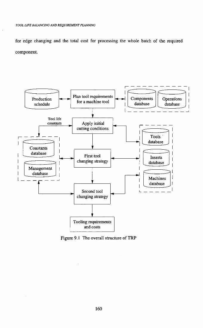
TOOL LIFE BALANCING AND REQUIREMENT PLANNING
for edge changing and the total cost for processing the whole batch of the required
component.
Production schedule
Tool life constants
J:
Constants database
Management database
Plan tool requirements for a machine tool
Apply initial cutting conditions
First tool changing strategy
Second tool changing strategy
Tooling requirements and costs
Components database
Operations database
r
Figure 9.1 The overall structure of TRP
Tools database
Inserts database
Machines database
160

TOOL UFE BALANCING AND REQUIREMENT PLANNING
Table 9.1 Weekly production schedule Plan Much. Comp. Material No. of Batch No.
Code code sub-class operations size batches
Day I CNC-1000 A ENS 5 100 6
B SS316 4 100 5
C ENS 3 250 2
Day 2 Machine X
Day 3 Machine Y
9.3 THE APPLICATION OF THE INITIAL MACHINING CONDITIONS
This section describes the considerations involved during the calculation of tool changes
required when applying the initial cutting data. To demonstrate the operation of TRP, it
is assumed that the machine tool CNC-1000 has been selected f rom Table 9.1 and the
planning of tooling requirements relates to component A. It must be noted that the same
procedure can be used for planning the machining of any set of components such as A, 5
and C.
The requirement is to produce 600 components of this type in 6 batches of 100 parts
each. The process plan for part A includes five operations and five tools as shown in
Table 9.2. The economic cutting velocity and the tool life value for each operation were
calculated separately using the first three modules of the system (TPO, TLP and TLA) .
For the f ive operations required to process component A, TRP retrieves the data shown
in Table 9.2 f rom the system's database. There are four medium roughing cuts and one
finishing operation with predicted tool l i fe values ranging f rom 5.2 to 14.63 min.
161

TOOL UFE BALANCING AND REQUIREMENT PLANNING
Table 9.2 he operations required to generate component A Operation
no.
Grade Type of
cut
V s Tsugg Tmod / D
1 TP20 M R 365 0.22 16.42 11.39 50.0 86.2
2 TP20 M R 350 0.25 14.25 8.53 50.0 78.0
3 TP20 M R 285 0.34 16.27 5.20 50.0 60.4
4 TP20 M R 300 0.24 31.85 12.93 50.0 48.4
5 TPIO F 400 0.13 17.00 14.63 50.0 46.0
For each operation shown in Table 9.2, TRP calculates the machining time, the number
of parts per cutting edge (mc), and the number of edges (Ng) needed to machine the
required batches using equations 9.4,9.5 and 9.7 respectively.
Operation 1
t2J = n Dl 3.14 X 86.2 X 50
1000 V s 1000 X 365 x 0.22 = 0.16854 min
mc J = int 11-39 \
= int = 67 parts 0.16854)
Operation 2
Ngl - int w q
^mc] + 0.99
J = int I — + 0.99 = 9 edges
67
3.14 X 78 x 50 . ?2,2 ~ — T T z — T T T =0.13995 mm
1000x350x0.25
( 8.53 \ mcy =mt ,
^ V0.13995J
Ne2 = 10 edges
= 60 parts
162

TOOL UFE BALANCING AND REQUIREMENT PLANNING
Operation 3
3.14 X 60.4 X 50 ^ . to 3 = = 0.09786 mm ^'"^ 1000 x 285 x 0.34
5.2 ^ m c 3 - i n t '• = 5 3 parts
A09786J ^
Ne3 = 12 edges
Operation 4
3.14 X 48.4 X 50 ^ . tjA = =0.10554 mm ^•^ 1000 x 300 x 0.24
12.93 \ mcd = int '• =122 parts
^ A10554)
Ne4 = 5 edges
Operation 5
^'^ 1000 x 400 x 0.13
. ( 14.63 A mc'; = int = 105 parts
^ {0.13888J ^
Ne4 = 6 edges
Table 9.3 shows the summary of the above calculations.
163
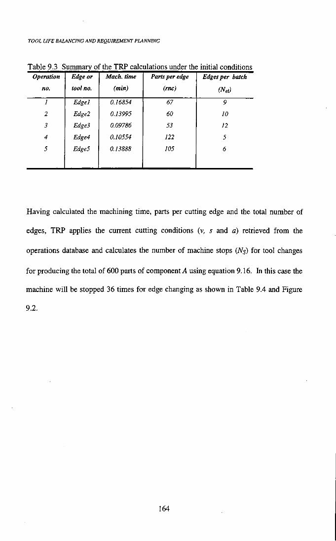
TOOL LIFE BALANCING AND REQUIREMENT PLANNING
Table 9.3 Summary o] F the TRP calculations under the initial conditions Operation Edge or Mach. time Parts per edge Edges per batch
no. tool no. (min) (mc) (Nei)
1 Edge] 0.16854 67 9
2 Edgel 0.13995 60 10
3 EdgeS 0.09786 53 12
4 Edge4 0.10554 122 5
5 EdgeS 0.13888 105 6
Having calculated the machining time, parts per cutting edge and the total number of
edges, TRP applies the current cutting conditions (v, s and a) retrieved f rom the
operations database and calculates the number of machine stops (A'^) for tool changes
for producing the total of 600 parts of component A using equation 9.16. In this case the
machine w i l l be stopped 36 times for edge changing as shown in Table 9.4 and Figure
9.2.
164

TOOL UFE BALANCING AND REQUIREMENT PLANNING
Table 9.4 Machine stoppages under the initial conditions Stop Incremental Accumulated Edge changed no. no. of parts no. of parts
0 0 0 Edgel, Edge2, EdgeS, Edge4, Edge5 1 53 53 Edge3 2 7 60 Edgel 3 7 67 Edgel 4 38 105 Edge5 5 1 106 Edge3 6 14 120 Edge2 7 2 122 Edge4 8 12 134 Edgel 9 25 159 EdgeS 10 21 180 Edge2 11 21 201 Edgel 12 9 210 Edge5 13 2 212 EdgeS 14 28 240 Edge2 15 4 244 Edge4 16 21 265 EdgeS 17 3 268 Edgel 18 32 300 Edge2 19 15 315 Edge5 20 3 318 EdgeS 21 17 335 Edgel 22 25 360 Edge2 23 6 366 Edge4 24 5 371 EdgeS 25 31 402 Edgel 26 18 420 Edge2, EdgeS 27 4 424 EdgeS 28 45 469 Edgel 29 8 477 EdgeS 30 3 480 Edge2 31 8 488 Edge4 32 37 525 EdgeS 33 5 530 EdgeS 34 6 536 Edgel 35 4 540 Edge2 36 43 583 EdgeS
Figure 9.2 is particularly informative since it reveals that there is a wide spread of edge
changing interruptions when producing part A. The edge changing time (tg) occurs 37
times and the machine stoppage time (f^) occurs 36 times.
165

• I
s tf)
c o T3 C o u 13 •a
X
X X 60 C
CO c
o
e 3 C
3 e 3 O
o "o Q
CO ao «! o
c
<N fi^ <n S> SJ s> s> 6e 645 645 645 N, I« !Q
E4 !«] E4 ,
OS
TOOL LIFE BALANCING AND REQUIREMENT PLANNING
Obviously, the effect of such frequent edge changing wi l l be seen when calculating the cost for producing the batches of component A. In order to calculate the cost values, TRP retrieves f rom the system's database the following values:
1. From the machine database, the cost rate of the selected machine {CNC-1000),
x = l £ / m i n .
2. From the inserts database, the inserts cost (TPIO, TP20) = £3.54
3. From the tools database, the tool holder (PCLNR2020-12A) cost = £38.33
The cost per cutting edge is calculated as follows [Maropoulos 1990]:
insert cost 1.3 x holder cost y = + = £ 1.3046
0.75 X number of cutting edges 400
The above correspond realistically to the tools and machine tool used.
The work set up time {tj) is dependent upon the size and weight of the workpiece, the
type and number of workholding devices and the type of the machine tool. For
example, small workpieces can be located in a self-centering chuck of a lathe in less
than 0.5 min. Larger workpieces which need a tailstock need longer to set. Finally, very
large workpieces machined on vertical boring machines may need several hours to
correctly locate and clamp on the machine tool's rotating bed. For the CNC-1000 lathe,
the work set up times were found to be ti = 0.3 min for small parts and = 1.0 min for
parts needing tailstock support.
167

TOOL LIFE BALANCING AND REQUIREMENT PLANNING
Equally variable can be the edge changing times and machine stoppage times as shown in Table 9.5. For the CNC-1000 lathe it was found that the average times of Table 9.5 were close to what was observed in practice and these were used for the calculation.
Table 9.5 Tool changing time
Rapid or simple Average or normal Slow or complex
tool change tool change tool change
ts = 0.3 min ts= 1.0 min ts = 1.5 min
te = 0.6 min te=l.5 min tg = 3.0 min
Finally, TRP calculates the cost under the initial machining conditions using equations
9.12, 9.13, 9.15 and 9.17 as follows:
Work set up cost (Ks) = 600 x 1 x 0.3 = £180
Machining cost (KM) = 600 X 1 [0.16854 + 0.13995 + 0.09786 + 0.10554 +
0.13888] = £390.46
Tool changing cost (KT) = 1 [36 X 1.0 + 1.5 X 37] = £91.5
Tool wear cost (Kw) = 1.3046 x 42 = £54.7932
The total machining cost per batch (Cb) = £716.753
Clearly, the initial tool changing practice suffers f rom two drawbacks:
• There is frequent tool change which must be communicated to the operator and
this may result in errors on the shop floor.
• Time is wasted because the set-up and machine stoppage times for each tool
change are counted separately since tool changes are sequential.
168

TOOL UFE BALANCING AND REQ UIREMENT PLANNING
The cutting velocity, feed rate and tool l i fe for minimum cost can be modified in order to result in an overall optimum cost for machining [Maropoulos 1989]. This can be achieved by one of the fol lowing methods:
• Replace the cutting edge before the end of its life.
• Change the cutting velocity and/or feed rate, thereby increasing tool life and
reducing the number of tool changes. In roughing operations, it may be
impossible to increase the cutting conditions due to some other constraints such
as machine power and it may not be practical to test all the machining constraints
at this stage [Maropoulos 1989].
Using this balancing theory [Maropoulos 1989], two new strategies for tool changing
optimization have been developed. The logic of the proposal is based on the
assumptions that the number of parts between tool changes must be constant and that
there must be enough edges to finish the required batch.
9.4 FIRST TOOL CHANGING STRATEGY
9.4.1 Identification of tool with least wear
From the retrieved operations, the cutting edge which can machine the maximum
number of parts (mCmax) by applying the present conditions is identified. Then, the ratio
of the total production (w q) to the maximum number of parts per cutting edge (mCmax)
is calculated. Obviously, this ratio (Ratiobatck) corresponds to the minimum number of
169

TOOL LIFE BALANCING AND REQUIREMENT PLANNING
edges required to complete the batch. This ratio can be calculated for the operation j, assuming it has produced the maximum number of parts as follows:
Operation i ( rncj = rnCmax)
R^tioi,atch = - ^ + 0.5 (9.18)
Adding 0.5 and taking the integer, the value of Ratiobawh is rounded to the nearest
integer. The modified number of parts (mCj^Mi) for this edge is calculated on this basis:
mcj^Ml=int ' wq ^
Ratio hatch (9.19)
The number of edges (Ngj^Mi) required to finish the whole batch considering the
modified number of parts can be calculated as follows:
N. ej,Ml = int w q
mCjMl + 0.99 (9.20)
The above value is rounded to the next higher integer number.
When the modified number of parts is greater than the original number of parts using
the retrieved conditions (mcj_Mi > rnCmax), the cutting conditions should be altered in
order to machine the new larger number of parts (mcj^Mi) either by reducing the cutting
velocity or the feed rate. I f the modified number of parts is less than the number of parts
using the initial conditions (mcj^Mi < rncmax)^ the cutting conditions should not be
modified (increased) to avoid violating the machining constraints.
170

TOOL LIFE BALANCING AND REQUIREMENT PLANNING
9.4.1.1 Modifying cutting velocity (v)
The modified cutting velocity (v/m;) used to machine the new larger number of parts
can be calculated as follows [Maropoulos 1989]:
_ f ^ g j , M 7 n D I
"'•"''[looocsO-''^' (9.20
9.4.1.2 Modifying feed rate (s)
The modified feed rate (sj^Mi) used to machine the new larger number of parts can be
calculated as follows:
^j.Ml -^ mCj^Ml K D I ^
1000 C v(^-^^">
1-1/p^ (9.22)
9.4.2 Modification of conditions for remaining tools
In order to keep a constant number of parts between edge changes, the modified number
of parts which can be machined by the remaining edges wi l l be computed by dividing
the new number o f parts {mcj^Mi) for the edge with the least wear (longest tool l ife) by
the fol lowing ratios: 1 : 2 : 3 etc. Another ratio {RatiOmdMi) is calculated between the
modified number of parts imcj^Mi) and the number of parts per edge for the remaining
edges required for processing the selected component. This ratio {RatiOmdMi) be
calculated for operation z as follows:
171

TOOL UFE BALANCING AND REQUIREMENT PLANNING
Operation i ( rnci)
where; i = 1, 2, 3, - m, and i ^ j i f j is the edge which produces the largest number of
parts.
RatiOmci,Ml=int + 0.5 (9.23)
This ratio is rounded to the nearest integer value.
In a similar manner as described in section 9.4.1, the modified real number of parts and
the required number of edges can be calculated using the following equations.
mCi_Ml=^nt ^ mCj^Ml ^
RatiOmci,Ml J (9.24)
mci Mi is rounded down to the nearest integer number.
Nei,Ml=int w q
{rnCi^Ml + 0.99 (9.25)
Nei^Mi is rounded to the next higher integer value.
I f mci Mi > mci, there w i l l be an increase in tool life to machine the re-calculated higher
number of parts (i.e., reduce v or s). The modified cutting conditions can be calculated
using equations 9.21 and 9.22. I f mci^Mi < rnci, the initial cutting data w i l l be used.
This process is repeated according to the number of operations required to machine the
selected component as w i l l be shown in the following example.
172

TOOL LIFE BALANCING AND REQUIREMENT PLANNING
9.4.3 An example to demonstrate the first method
In the example discussed in Section 9.3, edge 4 machines the maximum number of parts
(122 parts) as shown in Table 9.3. Therefore, using equation 9.18, Ratiobatch is
calculated as follows:
Operation 4 (rnc4 = 122 parts)
n • • (600 ^ ^ Ratioi,atch=int \J^ + 0.5 = 5
TRP calculates the modified number of parts and the required number of cutting edges
using equations 9.19 and 9.20.
. (600^ mc4^Mi - = 120 parts
Ne4,Mi = int ^ + 0.99 =5 edges
No alteration of cutting data is applied (mc4 > mc4_Mi)-
Operation 1 (rncj = 67 parts)
As discussed in section 9.4.2, the ratio (RatiOmci,Mi) is calculated between the
maximum modified number of parts {rnc4Mi= 120) and the number of parts {mci)
machined by this edge by applying the initial conditions, using equation 9.23.
(120 ^ RatiOmci, Ml =int — + 0.5 = 2
V 0 / J
The modified number of parts for this edge can be re-calculated using equation 9.24.
173

TOOL UFE BALANCING AND REQUIREMENT PLANNING
• (120\ f^ci.Ml =^«? = 60 parts
\ 2 J
The number of edges needed in this operation to finish 600 parts of component A can be
re-calculated using equation 9.25 as follows:
f600 \ NeiMi = int + 0.99 = 1 0 edges
\ 60 J
In this operation, the waste of carbide is 7 parts per cutting edge. This is because, the
number of parts this edge can machine under the initial machining conditions is reduced
by 7 compared with the modified number of parts resulted by applying the first tool
changing strategy (mci - mcj ^i = 7). The cutting conditions (v, s) cannot be modified
in this case to avoid violating the machining constraints (mcj^Mi < mcj).
Operation 2 (rnc2 = 60 parts)
(120 \ RatiOmc2,Ml=int -7^-^0.5 = 2
V oO J
• 120^ ^r. mc2,Mi = int = 60 parts
Ne2,Mi=int ^^^^ + 0.99 = 1 0 edges V 60
In this operation, the same cutting data w i l l be used. This is because mc2,Mi = mc2.
Operation 3 (rnc3 = 53 parts)
120 Ratio^c3Mi=int
V53 + 0.5 = 2
174

TOOL UFE BALANCING AND REQUIREMENT PLANNING
• 120^ . r . ^C3,Mi - ^^^ - 60 parts
^eSMi =int [ — + 0.99] = 10edges \ 60 J
TRP retrieves the tool l i fe constants for machining (ENS) free cutting steel using TP20
insert grade under semi-roughing conditions. This is because an alteration (reduction)
of cutting data is required in order to machine 60 parts instead of 53 parts. The initial
cutting conditions are v = 285 m/min and 5 = 0.34 mm/rev as shown in Table 9.2.
• Modifying v
The modified cutting velocity and the corresponding cutting time can be re-calculated
using equations 9.21 and 9.4 respectively.
(—J—] ( 60 X 3.14 X 60.4 x 50 \i-2.07993.
V3,M1 = 1000 X 26909.913 x 0.34^'^'^^^^'^.
= 252.48 m/min
3.14 x 60.4 x 50 . t2 3= = 0.11047 nun
' 1000 X 252.48 x 0.34
• Modifying s
The modified feed rate and the corresponding machining time cane be re-calculated
using equations 9.22 and 9.4 as follows:
( 1 ( 60 x 3.14 x 60.4 x 50 )[l-2.96237, ^ , , 0
S3.,Mi = , ^ ^-,r^r.•, =0.318 mm/rev 1000 X 26909.913 x 285^~^-^^^^^ )
3.14 X 60.4 X 50 . , . t2 3= = 0.10463 min
' 1000 X 285 X 0.318
175

TOOL UFE BALANCING AND REQUIREMENT PLANNING
As expected, the cutting velocity and feed rate are reduced f rom their original values in
order to increase tool l i fe to allow the machining of 60 parts instead of 53 parts.
Operation 5 (mcg = 105 parts)
fnn \ = 1
fl20 RatiOmc5,Ml=int [ j ^ + 0-5j
• 120^ .^r. mc5^Mi=int =120 parts
f600 A Ne5.Mi=int -— + 0.99 = 5 edges
\.120 J
Again, TRP retrieves the tool l i fe constants for machining free cutting steel CEN8) using
TPIO insert grade under finishing conditions. This is because an alteration of cutting
data is required in order to machine 120 parts instead of 105 parts. The initial cutting
data is V = 400 m/min and .s = 0.13 mm/rev as shown in Table 9.2.
• Modifying v
The modified cutting velocity and cutting time are re-calculated as follows:
l_ ( 120 X 3.14 X 46 x 50 \i-2.93474, „ . , .
V5,Mi= , ^ ,oon = 373.89 m/mm UOOO X 4.350624E8 x O.B^'^-^^^^
3.14 x 46 x 50 ^ , , o c o • t2 5= = 0.14858 mm
' 7000 X 373.89 x 0.13
lie

TOOL UFE BALANCING AND REQUIREMENT PLANNING
• Modifying s
In the case of modifying s, the modified feed rate and cutting time can be re-calculated
as follows:
S5.MI ~ 120 X 3.14 X 46 X 50
{1000 X 4.350624E8 x 400^-2-93474 1-0.1839 = 0.153 mm/rev
3.14 x 46 x 50 . t2 5= =0.11801 min
' 1000 X 400 X 0.153
The modified cutting velocity is lower than the original value. However, this is not the
case for the feed rate which is increased from 0.13 mm/rev to 0.153 mm/rev in order to
machine 120 parts instead of 105 parts. This phenomenon can have very useful
applications in machining economics and was first observed by Maropoulos (1989). Its
explanation lies in the fact that the exponent of the feed rate in Taylor's equation is less
than one for finishing operations. In this particular case ~ - ^9.
Table 9.6 shows a summary of the above calculations resulting from applying the first
tool balancing strategy.
Table 9.6 Summary of RP calculations by applying the first strategy Op. Parts per edge Edges per batch V s Mod. V Mod. s no Initial Final Initial Final m/min mm/rev m/min mm/rev 1 67 60 9 10 365 0.22 No change No change
2 60 60 10 10 350 0.25 No change No change
3 53 60 12 10 285 0.34 252.48 0.318
4 122 120 5 5 300 0.24 No change No change
5 105 120 . 6 5 400 0.13 373.89 0.153
177

TOOL LIFE BALANCING AND REQUIREMENT PLANNING
TRP calculates the number of machine stops by applying this balancing strategy using equation 9.16 as shown in Table 9.7 and Figure 9.3. It is clear that the number of machine stops for edge changing is reduced by 27 when compared with the results by applying the retrieved machining data (36 stops) as discussed in section 9.3 and shown in Table 9.4 and Figure 9.2. More importantly, the wide spread of tool changes shown in Figure 9.2 is replaced by a clustering of changes by producing a constant number of parts. Multiple edge changes are executed in every machine stoppage, thereby reducing the unproductive time due to tool changing.
Table 9.7 Machine stoppages using the first strategy Stop no. Incremental Accumulated Edge changed
parts parts
0 0 0 Edgel, Edge2, Edge3, Edge4, EdgeS
J 60 60 Edgel, Edge2, Edge3
2 60 120 Edgel, Edge2, Edge3, Edge4, EdgeS
3 60 180 Edgel, Edge2, Edge3
4 60 240 Edgel, Edge2, EdgeS, Edge4, EdgeS
5 60 300 Edgel, Edge2, Edge3
6 60 360 Edgel, Edge2, Edge3, Edge4, EdgeS
7 60 420 Edgel, Edge2, Edge3
8 60 480 Edgel, Edge2, Edge3, Edge4, EdgeS
9 60 540 Edgel, Edge2, Edge3
178
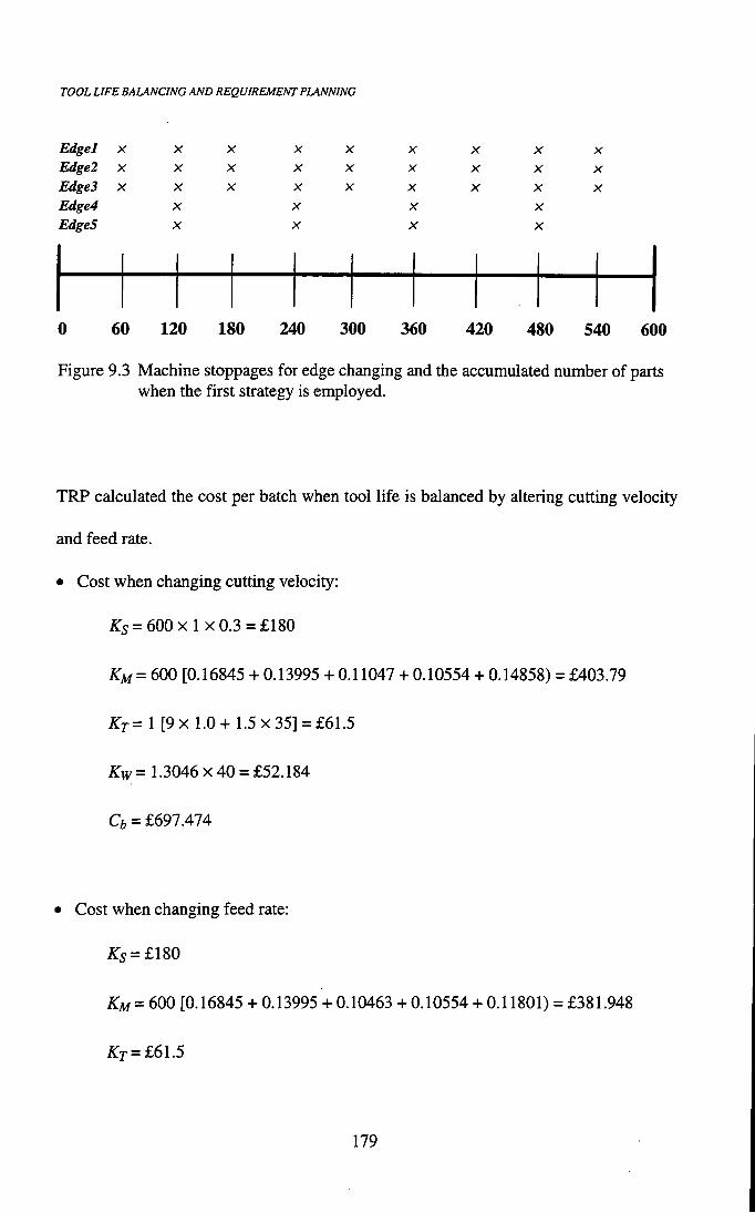
TOOL UFE BALANCING AND REQUIREMENT PLANNING
Edgel X X X X X X X X X
Edge2 X X X X X X X X X
EdgeS X X X X X X X X X
Edge4 X X X X
EdgeS X X X X
0 60 120 180 240 300 360 420 480 540 600
Figure 9.3 Machine stoppages for edge changing and the accumulated number of parts when the first strategy is employed.
TRP calculated the cost per batch when tool life is balanced by altering cutting velocity
and feed rate.
• Cost when changing cutting velocity:
/$:5 = 600x 1 x0.3 = £180
/ i : M = 600 [0.16845 + 0.13995 + 0.11047 + 0.10554 + 0.14858) = £403.79
KT= 1 [9 X 1.0+ 1.5x35] = £61.5
K^N= 1.3046x40 = £52.184
Q = £697.474
• Cost when changing feed rate:
^5 = £180
KM = 600 [0.16845 + 0.13995 + 0.10463 + 0.10554 + 0.11801) = £381.948
/i:r=£61.5
179
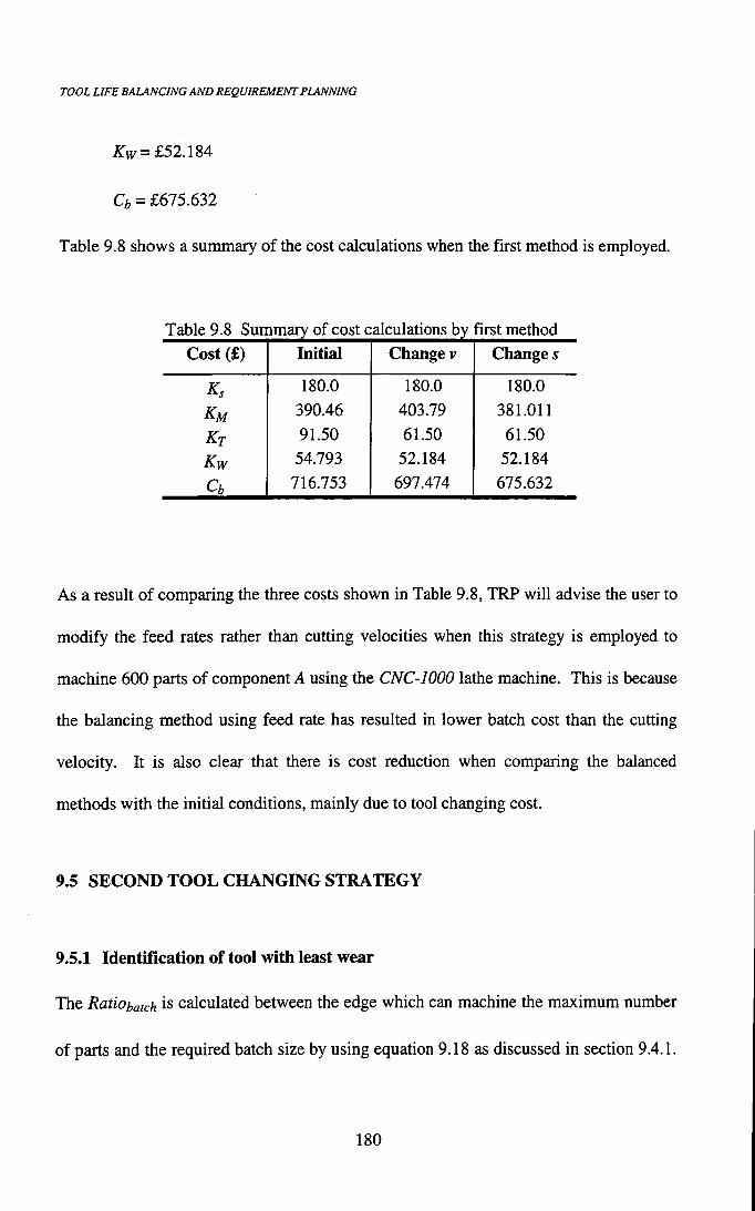
TOOL UFE BALANCING AND REQUIREMENT PLANNING
Kw = £52.\S4 Cb = £675.632
Table 9.8 shows a summary of the cost calculations when the first method is employed.
Table 9.8 Summary of cost calculations by first method Cost (f) Initial Change v Change s
Ks 180.0 180.0 180.0
KM 390.46 403.79 381.011
Kf 91.50 61.50 61.50
Kw 54.793 52.184 52.184
Cb 716.753 697.474 675.632
As a result of comparing the three costs shown in Table 9.8, TRP will advise the user to
modify the feed rates rather than cutting velocities when this strategy is employed to
machine 600 parts of component A using the CNC-1000 lathe machine. This is because
the balancing method using feed rate has resulted in lower batch cost than die cutting
velocity. It is also clear that there is cost reduction when comparing the balanced
methods with the initial conditions, mainly due to tool changing cost.
9.5 SECOND T O O L CHANGING S T R A T E G Y
9.5.1 Identification of tool with least wear
The Ratiobatch is calculated between the edge which can machine the maximum number
of parts and the required batch size by using equation 9.18 as discussed in section 9.4.1.
180

TOOL LIFE BALANCING AND REQUIREMENT PLANNING
The modified number of parts {mcjMi), the required number of cutting edges {Ngj^Ml) and the cutting time (t2j) can be re-calculated for this edge using equations 9.19, 9.20 and 9.4 respectively.
I f the modified number of parts is greater than the original number by applying the
initial conditions (mcj^M2 > rncj), the cutting conditions can be modified using equations
9.21 and 9.22. Otherwise, no alteration of cutting data is applied.
9.5.2 Modification of conditions for remaining tools
In order to keep a constant number of parts between edge changes, the number of parts
(mci^Mi) which can be machined by the remaining edges are re-calculated by dividing
the modified maximum number of parts {mcj_M2) per edge, by the following ratios: 1 :
1.5 : 2 : 2.5 etc. The following ratio is calculated:
^mcj^M2^^^^ + 0:5\ (9.26)
By adding 0.5 and taking the integer, this ratio is rounded to the nearest integer number.
The modified number of parts (mc,,^2) is calculated using the following equation:
( mCi^M2=^nt
mCjM2 (9.27)
^{RatiOmci,M2^2)^
By taking the integer, the number of parts calculated by equation 9.27 is rounded down
to the nearest integer number. The modified number of edges {Nei,M2) is calculated as
follows:
181

TOOL UFE BALANCING AND REQUIREMENT PLANNING
^ei,M2 =int (9.28)
The calculated number of edges is rounded to the next integer number.
Again i f mciMi > "^Q^ the modified machining conditions are calculated using
equations 9.21 and 9.22. Otherwise, no alteration of cutting data is applied. This
process is repeated for the retrieved number of operations as will be shown in the next
example.
9.5.3 An example to demonstrate the second method
For the example discussed in sections 9.3 and 9.4.3, the Ratiobatch is calculated for edge
4 since it produces the maximum number of parts (122 parts) using equation 9.18.
(600 ^ Ratiotatch'^int T^ + (^-^ =5
The modified number of parts and the required number of edges are calculated using
equations 9.19 and 9.20.
(600\ mc4M2 = int = 120 parts
Ne4M2 = int + 0.99] = 5 edges \1ZU J
In this operation, no alteration of cutting data is applied. This is because the number of
parts per edge is reduced by 2 {mc4 - mc4 M2 = 2).
182

TOOL LIFE BALANCING AND REQUIREMENT PLANNING
Operation 1 (rncj = 67 parts)
Using equation 9.26, the following ratio is calculated:
{fl20 ^ 1 RatiOmci,M2=int — - x 2 +0.5 = 4
IV 0/ J J
The modified number of parts and the required number of edges can be calculated using
equations 9.27 and 9.28 as follows:
• (i^o\ mciM2 =int = 60 parts
\4/2)
f 600 A NeiM2= int + 0.99 =10 edges
\60 J
The waste of carbide is 7 parts per cutting edge. This is because the number of parts this
edge can machine is reduced by 7. Again, no alteration of cutting data is applied (rrac; >
Operation 2 (rnc2 = 60 parts)
{(120 \ 1 Ratiomc2,M2 = j l ^ — X 2 j + 0.5^ = 4
. 120^ mc2,M2=int =60parts
Ne2.M2=int ^ + 0.99 =10edges 60
For this operation, the same initial cutting data will be used since mc2,M2 = mc2-
183

TOOL UFE BALANCING AND REQUIREMENT PLANNING
Operation 3 (rnc3 = 53 parts)
If 120 RatiOmc3,M2 =^'«^ V53
x2\ + 0.5[ =5
mc3^M2=int — — =48 parts
Ne3.M2=int ^ + 0-99^ = 13 edges
The waste of carbide is 5 parts per edge. This is because the number of parts this edge
can machine is reduced by 5 (mcj - mcs^Mi = 5). Again, no alteration of cutting data is
applied (mcs > mcs MT)-
Operation 5 (rncs = 105 parts)
\( 120 \ 1 Ratio^c5,M2 = int j l ^ — X 2 j + 0.5\ = 2
• (120\ mc5M2=^nt =120parts
\2/2)
Ne5M2 = int + 0.99] = 5 edges \120 )
An alteration of cutting data is required in order to machine 120 parts instead of 105
parts.
• Modifying v
The modified cutting velocity and the corresponding cutting time are re-calculated using
equations 9.21 and 9.4.
184

TOOL LIFE BALANCING AND REQUIREMENT PLANNING
V5,M2 = 120 X 3.14 X 46 X 50
1000 X 4.350624E8 x 0.13^-^-^^^^
1 1-2.93474 = 373.89 m/min
3.14 x 46 x 50 . t2 5 = = 0.14858 min
' 1000 X 373.89 x 0.13
• Modifying s
In the case of modifying s, the new feed rate and the corresponding cutting time can be
re-calculated using equations 9.22 and 9.4.
1
S5,M2 = 120 X 3.14 X 46 X 50
1000 X 4.350624E8 x 400^~^-^^"^^"^) 1-0.1839 = 0.153 mm/rev
3.14 x 46 x 50 ^ , , o n i •
5 = =0.11801 min ' 1000 X 400 X 0.153
Table 9.9 shows a summary of this calculations when the second tool balancing strategy
is employed.
Table 9.9 Summary of TRP calculations by applying the second strategy Op. Parts per edge Edges per batch V s Mod. V Mod. s
no Initial Final Initial Final m/min mm/rev m/min mm/rev
1 67 60 9 10 365 0.22 No change No change
2 60 60 10 10 350 0.25 No change No change
3 53 48 12 13 285 0.34 No change No change
4 122 120 5 5 300 0.24 No change No change
5 105 120 6 5 400 0.13 373.89 0.153
185

TOOL LIFE BALANCING AND REQUIREMENT PLANNING
As with the first strategy, the tool requirement planning and balancing module (TRP) calculates the number of machine stops as shown in Table 9.10 and Figure 9.4. The second method results in 19 machine stoppages and 38 insert changes.
Table 9.10 Machine stoppages using the second strategy Stop no.
Incremental parts
Accumulated parts
Edge changed
0 0 0 Edgel, Edge2, Edge3, Edge4, Edge5
1 48 48 Edge3
2 12 60 Edgel, Edge2
3 36 96 Edge3
4 24 120 Edgel,Edge2, Edge4, EdgeS
5 24 144 Edge3
6 36 180 Edgel, Edge2
7 12 192 Edge3
8 48 240 Edgel, Edge2, Edge3, Edge4, EdgeS
9 48 288 Edge3
10 12 300 Edgel, Edge2
11 36 336 Edge3
12 24 360 Edgel,Edge2, Edge4, Edge5
13 24 384 Edge3
14 36 420 Edgel, Edge2
15 12 432 Edge3
16 48 480 Edgel,Edge2, Edge3, Edge4, Edge5
17 48 528 Edge3
18 12 540 Edgel, Edge2
19 36 576 Edge3
186
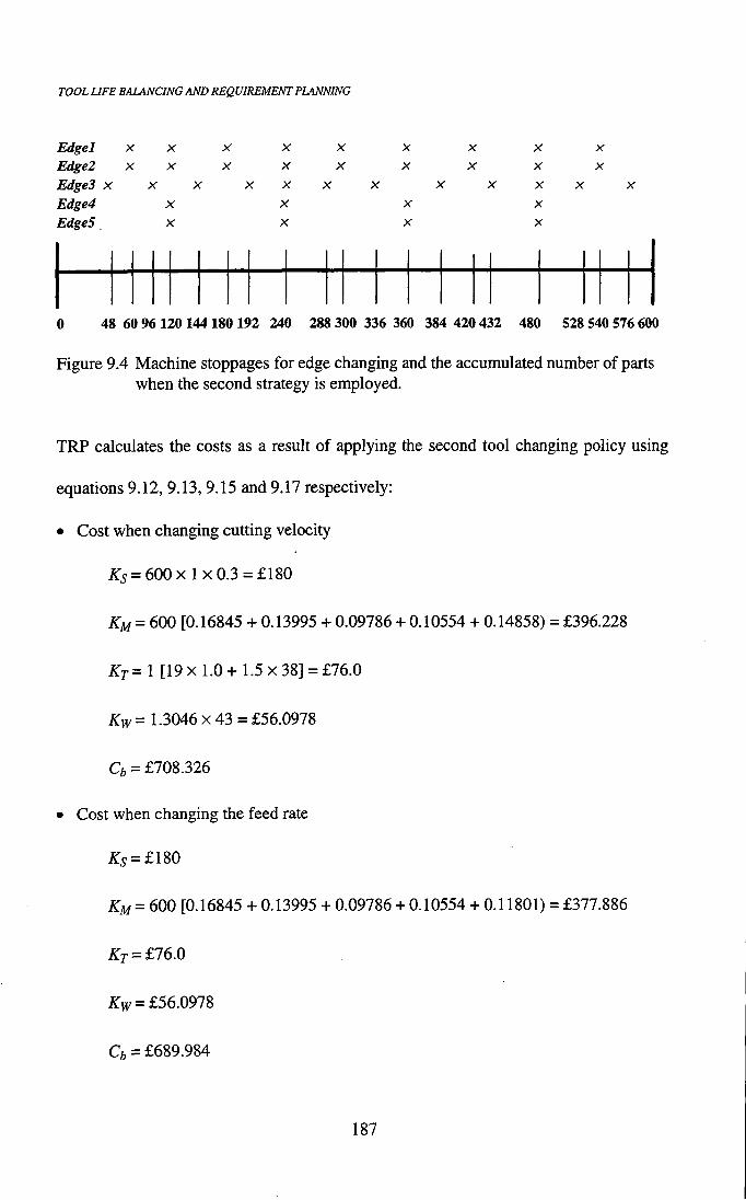
TOOL UFE BALANCING AND REQUIREMENT PLANNING
Edgel X X X X X X X X X
Edgel X X X X X X X X X
EdgeS X X X X X X X X X X X
Edge4 X X X X
EdgeS X X X X
0 48 60 96 120144180 192 240 288 300 336 360 384 420 432 480 528 540 576600
Figure 9.4 Machine stoppages for edge changing and the accumulated number of parts when the second strategy is employed.
TRP calculates the costs as a result of applying the second tool changing policy using
equations 9.12, 9.13,9.15 and 9.17 respectively:
• Cost when changing cutting velocity
/s:5 = 600x 1x0.3 = £180
KM = 600 [0.16845 + 0.13995 + 0.09786 + 0.10554 + 0.14858) = £396.228
KT= 1 [19 x 1.0 + 1.5 X 38] = £76.0
Kw= 1.3046x43 = £56.0978
Cb = £708.326
• Cost when changing the feed rate
is:5 = £180
/ S : M = 600 [0.16845 + 0.13995 + 0.09786 + 0.10554 + 0.11801) = £377.886
KT = £76.0
Kw = £56.091S
Cfc = £689.984
187
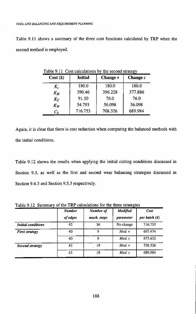
TOOL LIFE BALANCING AND REQUIREMENT PLANNING
Table 9.11 shows a summary of the three cost functions calculated by TRP when the
second method is employed.
Table 9.11 Cost calculations by the second strategy Cost (£) Initial Change v Change s
Ks 180.0 180.0 180.0
KM 390.46 396.228 377.886
Kf 91.50 76.0 76.0
Kw 54.793 56.098 56.098
Cb 716.753 708.326 689.984
Again, it is clear that there is cost reduction when comparing the balanced methods with
the initial conditions.
Table 9.12 shows the results when applying the initial cutting conditions discussed in
Section 9.3, as well as the first and second wear balancing strategies discussed in
Section 9.4.3 and Section 9.5.3 respectively.
Table 9.12 Summary of the TRP calculations for the three strategies Number Number of Modified Cost
of edges much, stops parameter per batch (£)
Initial conditions 42 36 No change 716.753
First strategy 40 9 Mod. V 697.474
40 9 Mod. s 675.632
Second strategy 43 19 Mod. V 708.326
43 19 Mod. s 689.984
188

TOOL LIFE BALANCING AND REQUIREMENT PLANNING
By comparing the results from the three strategies shown in Table 9.12, it is clear that the cost in the first and second strategies are less than the initial case. Furthermore, the two balancing strategies resulted in minimum cost by modifying the feed rates of operations. TRP will advise the user to consider implementing the first tool changing strategy with modified feed rates for machining 600 parts of component A using the CNC-1000 lathe machine.
Apart from the optimization of tool changing, TRP calculates the carbide (or
consumable tooling) requirements for the production schedule under consideration.
Table 9.12 summarises the cutting edges required for each one of the three methods. If
the first strategy is selected there is a total requirement for 40 edges and Table 9.6 shows
the exact requirements per operation or tool. In the previous Chapters, the integrated
tool life prediction and assessment methods using multiple regression have been shown
to address successfully the difficult problem of tool life prediction and control. The
application of these methods will allow the accurate planning of tool requirements and
this wi l l improve machining efficiency and reduce carbide costs.
9.6 E X A M P L E S TO DEMONSTRATE T H E TRP OPERATION
9.6.1 Example 1
The requirement is to produce 500 parts of the component B shown in Table 9.1. TRP
retrieves the four semi-roughing operations required to generate this component as
shown in Table 9.13. The predicted tool life ranging from 9.42 to 19.15 min.
189

TOOL LIFE BALANCING AND REQUIREMENT PLANNING
Table 9.13 The operations required to generate component B Operation
no. Grade Type of
cut V s ^sugg / D
1 TP35 M R 100 0.36 5.29 12.59 50 61.0
2 TP35 M R 105 0.35 4.29 11.69 50 51.0
3 TP35 M R 110 0.29 3.51 19.15 50 39.0
4 TP35 M R 130 0.3 1.71 9.42 50 21.4
For each operation, TRP calculated the machining time, the number of parts per edge
and the required number of edges to machine 500 parts of this component. The summary
of these calculations are shown in Table 9.14.
Table 9.14 Summary of the TRP calculations under the initial conditions Operation
no. Edge or tool no.
Much, time (min)
Parts per edge (mc)
Edges per batch (Nei)
1 Edgel 0.26603 47 11
2 Edge2 0.21788 53 10
3 Edge3 0.19194 99 6
4 Edge4 0.08615 109 5
Under the present cutting conditions, the edge changing time occurs 28 times and the
machine stoppage time occurs 28 times as shown in Table 9.15 and Figure 9.5.
190
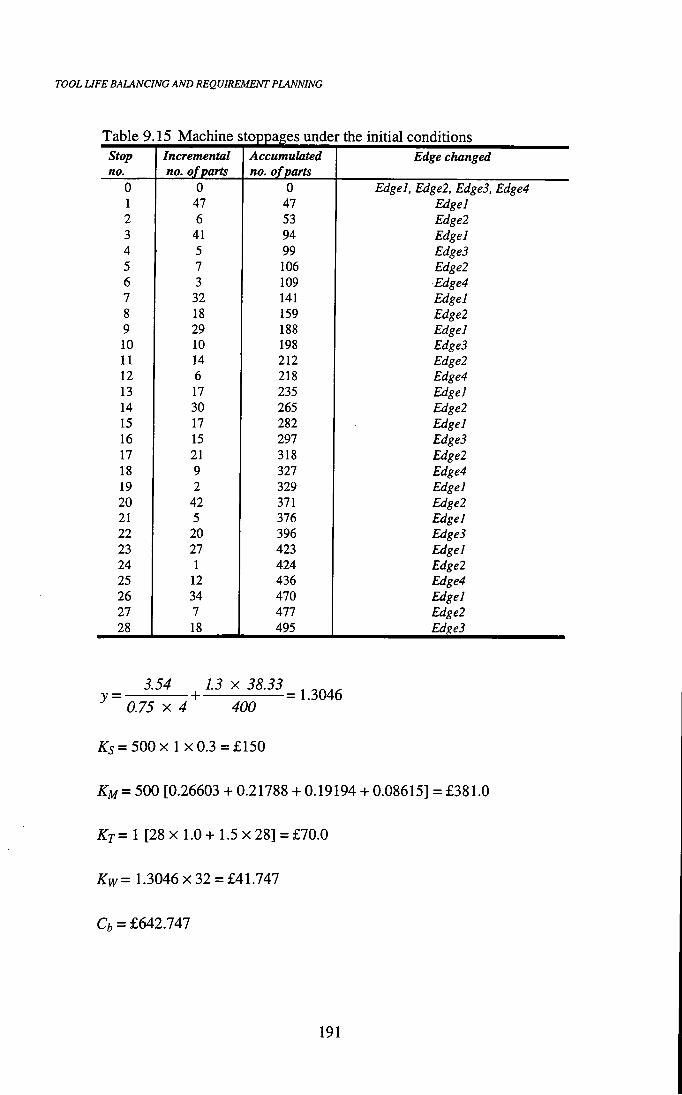
TOOL UFE BALANCING AND REQUIREMENT PLANNING
Table 9.15 Machine; the initial conditions Stop Incremental Accumulated Edge changed no. no. of parts no. o f parts
0 0 0 Edgel, Edge2, EdgeS, Edge4 1 47 47 Edgel 2 6 53 Edge2 3 41 94 Edgel 4 5 99 EdgeS 5 7 106 Edge2 6 3 109 Edge4 7 32 141 Edgel 8 18 159 Edge2 9 29 188 Edgel 10 10 198 EdgeS 11 14 212 Edge2 12 6 218 Edge4 13 17 235 Edge] 14 30 265 Edge2 15 17 282 Edgel 16 15 297 EdgeS 17 21 318 Edge2 18 9 327 Edge4 19 2 329 Edgel 20 42 371 Edge2 21 5 376 Edgel 22 20 396 EdgeS 23 27 423 Edgel 24 1 424 Edge2 25 12 436 Edge4 26 34 470 Edgel 27 7 477 Edge2 28 18 495 Edges
3.54 , 1.3 X 38.33 ^ y = —— - + — = 1.3046
0.75 X 4 400
^5 = 500x 1 X 0.3 =£150
KM = 500 [0.26603 + 0.21788 + 0.19194 + 0.08615] = £381.0
KT= 1 [28 X 1.0+ 1.5x28] = £70.0
Kw= 1.3046x32 = £41.747
Cb = £642.747
191
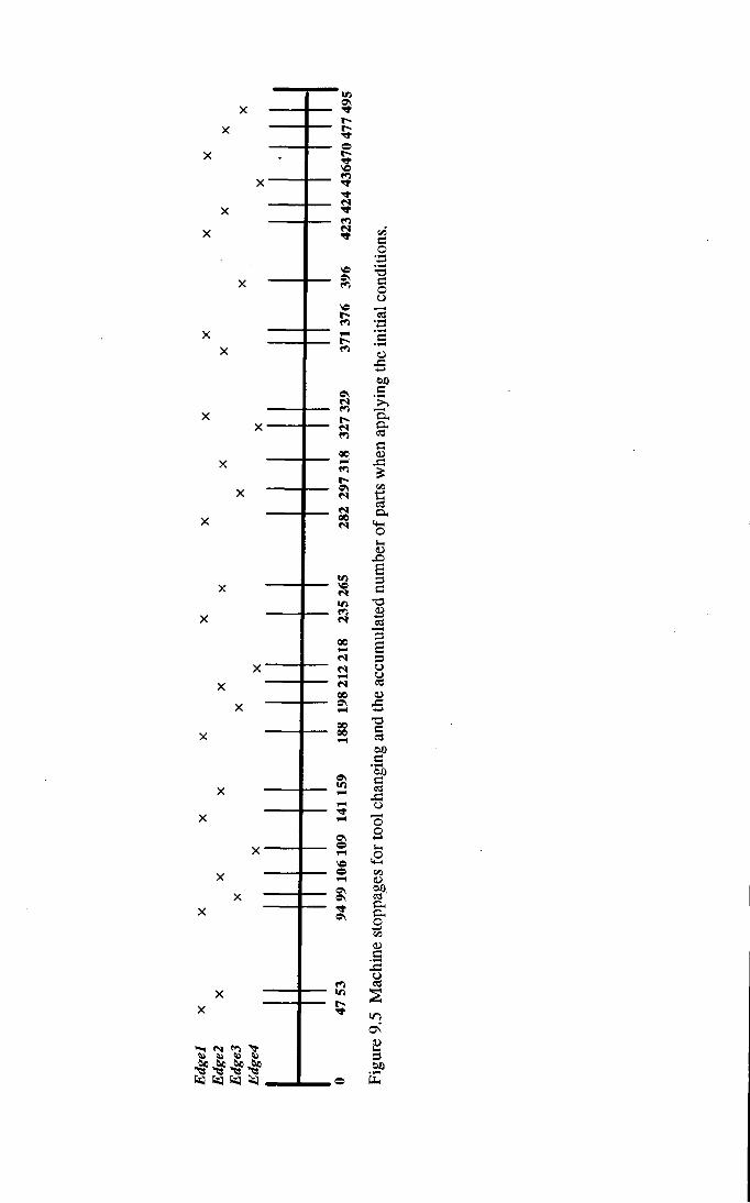
"-r fM <n > s, j> to
^ TJS ^ ^ Ct3 C« fej .
OS
ve
90 0\
00 00
5!
o
©
» 5 c o •a
O o
c
a,
c
O H
o
B 3 G I 3
s 3
i .c
c c euo G
o
I o
c • •-1
o
m
O N
3
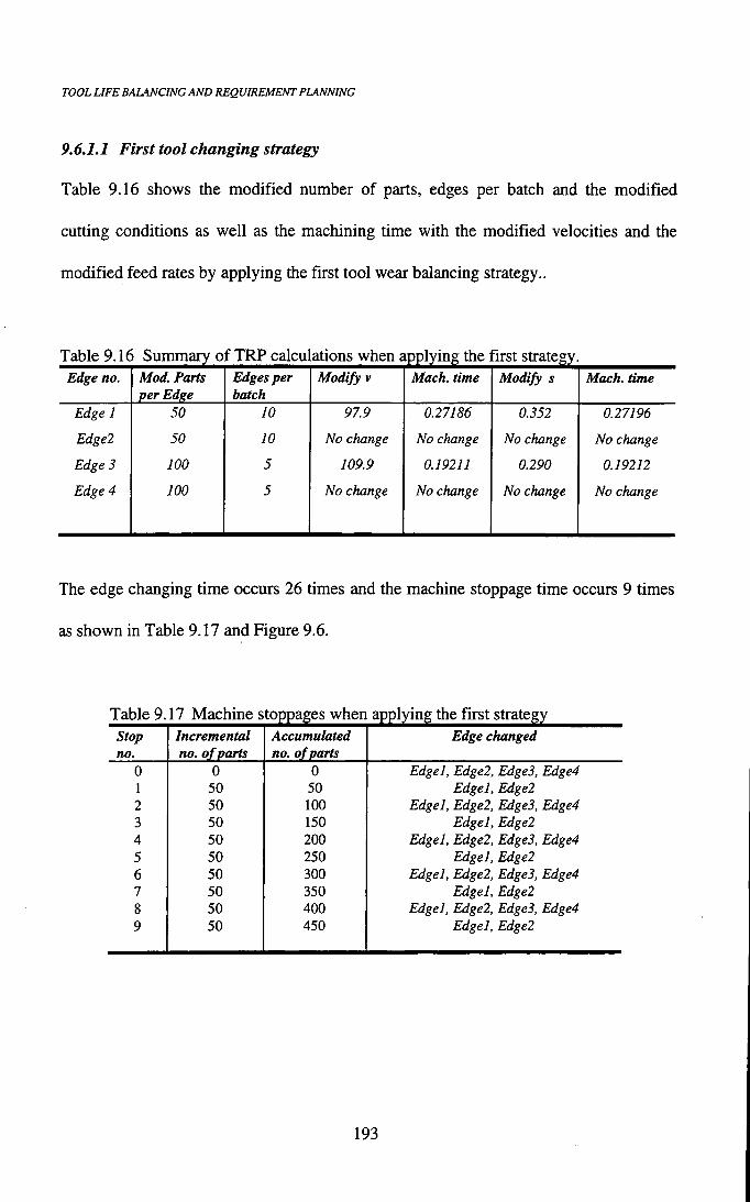
TOOL LIFE BALANCING AND REQUIREMENT PLANNING
9.6.1.1 First tool changing strategy
Table 9.16 shows the modified number of parts, edges per batch and the modified
cutting conditions as well as the machining time with the modified velocities and the
modified feed rates by applying the first tool wear balancing strategy..
Table 9.16 Summary of TRP calcul ations when applying the 1 irst strategy. Edge no. Mod. Parts
per Edge Edges per batch
Modify V Mach. time Modify s Mach. time
Edge 1 50 10 97.9 0.27186 0.352 0.27196
Edge! 50 10 No change No change No change No change
Edge 3 100 5 109.9 0.19211 0.290 0.19212
Edge 4 100 5 No change No change No change No change
The edge changing time occurs 26 times and the machine stoppage time occurs 9 times
as shown in Table 9.17 and Figure 9.6.
Table 9.17 Machine stoppages when applying the first strategy Stop Incremental Accumulated Edge changed no. no. of parts no. of parts
0 0 0 Edgel, Edge2, EdgeS, Edge4 1 50 50 Edgel, Edge2 2 50 100 Edgel, Edge2, Edge3, Edge4 3 50 150 Edgel, Edge2 4 50 200 Edgel, Edge2, Edge3, Edge4 5 50 250 Edgel, Edge2 6 50 300 Edgel, Edge2, Edge3, Edge4 7 50 350 Edgel, Edge2 8 50 400 Edgel, Edge2, Edge3, Edge4 9 50 450 Edgel, Edge2
193

TOOL LIFE BALANCING AND REQUIREMENT PLANNING
Edgel Edge! Edges Edge4
X
X
X
X
X
X
X
X
X
X
X
X
X
X
X
X
X
X
X
X
X
X
X
X
X
X
0 50 100 150 200 250 300 350 400 450 500
Figure 9.6 Machine stoppages for edge changing and the accumulated number of parts.
a) Cost when modifying v
is:5 = 500x 1 x0.3 = £150
KM = 500 [0.27186 + 0.21788 + 0.19211 + 0.08615) = £384.0
isTr = 1 [9 X 1.0 + 1.5 X 26] = £48.0
Kw= 1.3046x30 = £39.138
Cfc = £621.138
b) Cost when modifying s
is: = 500 X 1 X 0.3 = £150
KM = 500 [0.27196 + 0.21788 +0.19212 + 0.08615) = £384.05
is:7-= 1 [9 X 1.0 + 1.5 X 26] = £48.0
Kw= 1.3046x30 = £39.138
Ct = £621.188
194

TOOL UFE BALANCING AND REQUIREMENT PLANNING
9.6.1.2 Second tool changing strategy
Table 9.18 shows the modified number of parts, edges per batch and the modified
cutting conditions with the corresponding machining time calculated by the second
strategy.
Table 9.18 Summary of TRP calcu] ations when applying the second strategy. Edge no. Mod. Parts
per Edge Edges per batch
Modify V Mach. time Modify s Mach. time
Edge 1 50 10 97.9 0.27186 0.352 0.27196
Edgel 50 10 No change No change No change No change
Edge 3 100 5 109.9 0.19211 0.290 0.19212
Edge 4 100 5 No change No change No change No change
The edge changing time occurs 26 times and the machine stoppage time occurs 9 times
as shown in Table 9.19 and Figure 9.7.
Table 9.19 Machine stoppages when applying the second strategy Stop Incremental Accumulated Edge changed no. no. of parts no. of parts
0 0 0 Edgel, Edge2, Edge3, Edge4 1 50 50 Edgel, Edge2 2 50 100 Edgel, Edge2, EdgeS, Edge4 3 50 150 Edgel, Edge2 4 50 200 Edgel, Edge2, Edge3, Edge4 5 50 250 Edgel, Edge2 6 50 300 Edgel, Edge2, EdgeS, Edge4 7 50 350 Edgel, Edge2 8 50 400 Edgel, Edge2, EdgeS, Edge4 9 50 450 Edgel, Edge2
195

TOOL LIFE BALANCING AND REQUIREMENT PLANNING
Edgel Edgel Edges Edge4
X
X
X
X
X
X
X
X
X
X
X
X
X
X
X
X
X
X
X
X
X
X
X
X
0 50 100 150 200 250 300 350 400 450 500
Figure 9.7 Machine stoppages for edge changing and the accumulated number of parts.
a) Cost when modifying v
/s:5 = 500x 1 x0.3 = £150
KM = 500 [0.27186 + 0.21788 + 0.19211 + 0.08615) = £384.0
isTy = 1 [9 X 1.0 + 1.5 X 26] = £48.0
Kw= 1.3046x30 = £39.138
Ci = £621.138
b) Cost when modifying s
Ks = 500x 1 x0.3 =£150
KM = 500 [0.27196 + 0.21788 +0.19212 + 0.08615) = £384.05
KT^ 1 [9 X 1.0+ 1.5x26] = £48.0
Kw= 1.3046x30 = £39.138
Ci, = £621.188
196

TOOL UFE BALANCING AND REQUIREMENT PLANNING
Finally, the user can select any tool wear balancing strategy to be used to produce 500 parts of component B using CNC-1000 machine. This is because both strategies resulted in the same cost as shown in Table 9.20.
Table 9.20 Sunmiary of the TRP calculations for the three ;ies Number Number of Modified Cost
of edges mach. stops parameter per batch (£)
Initial conditions 32 28 No change 642.747
First strategy 30 9 Mod. V 621.138
30 9 Mod. s 621.188
Second strategy 30 9 Mod. V 621.138
30 9 Mod. s 621.188
9.6.2 Example 2
The requirement is to produce 500 parts of the component C shown in Table 9.1. TRP
retrieves the operations required to generate this component as shown in Table 9.21.
The predicted tool life ranging from 4.52 to 8.45 min.
Table 9.21 The operations required to generate component C Operation
no.
Grade Type of
cut
V s ^sugg Tmod / D
1 TP20 M R 370 0.3 6.90 4.52 90 77.6
2 TP20 M R 320 0.28 15.93 7.30 90 58.4
3 TP20 F 420 0.14 5.98 . 8.45 90 55.4
197

TOOL LIFE BALANCING AND REQUIREMENT PLANNING
For each operation, TRP calculated the machining time, the number of parts per edge and the required number of edges to machine 500 parts of this component. The summary of these calculations are shown in Table 9.22.
Table 9.22 Summary of the TRP calculations under the initial conditions Operation Edge or Mach. time Parts per edge Edges per batch
no. tool no. (min) (mc) (Nei)
1 Edgel 0.19757 22 23
2 Edge2 0.18419 39 13
3 EdgeS 0.26626 31 17
Under the present cutting conditions, the edge changing time occurs 50 times and the
machine stoppage time occurs 50 times as shown in Table 9.23. Figure 9.8 shows the
frequency of machine stoppages for producing 250 parts of component C.
3.54 1.3 X 38.33 , y = + = 1.3046
0.75 X 4 400
Ks = 500x1x0.3 = £150
KM=500 [0.19757 + 0.18419 + 0.26626) = £324.01
KT=\ [50X 1.0+ 1.5x50] = £125.0
Kw= 1.3046x53 = £69.144
Q = £668.154
198

TOOL LIFE BALANCING AND REQUIREMENT PLANNING
Table 9.23 Machine stoppages under the initial conditions Stop Incremental Accumulated Edge changed no. no. of parts no. of parts
0 0 0 Edgel, Edge2, EdgeS 1 22 22 Edgel 2 9 31 EdgeS 3 8 39 Edge2 4 5 44 Edgel 5 18 62 EdgeS 6 4 66 Edgel 7 12 78 Edge2 8 10 88 Edgel 9 5 93 EdgeS 10 17 110 Edgel 11 7 117 Edge2 12 7 124 EdgeS 13 8 132 Edgel 14 22 154 Edgel 15 1 155 EdgeS 16 1 156 Edge2 17 20 176 Edgel 18 10 186 EdgeS 19 9 195 Edge2 20 3 198 Edgel 21 19 217 EdgeS 22 3 220 Edgel 23 14 234 Edge2 24 8 242 Edgel 25 6 248 EdgeS 26 16 264 Edgel 27 9 273 Edge2 28 6 279 EdgeS 29 7 286 Edgel 30 22 308 Edgel 31 2 310 EdgeS 32 2 312 Edge2 33 18 330 Edgel 34 11 341 EdgeS 35 10 351 Edge2 36 1 352 Edgel 37 20 372 EdgeS 38 2 374 Edgel 39 16 390 Edgel 40 6 396 Edgel 41 7 403 EdgeS 42 15 418 Edgel 43 11 429 Edgel 44 5 434 EdgeS 45 6 440 Edgel 46 22 462 Edgel 47 3 465 EdgeS 48 3 468 Edgel 49 16 484 Edgel 50 12 496 EdgeS
199

<S PT)
s> s> s» fcjj 6* 6 a
Ct] Ef] ,
X)
1/1 9\
e
ac X
s
3 O
i
'Si c ca x: o o o
o
c
00
a
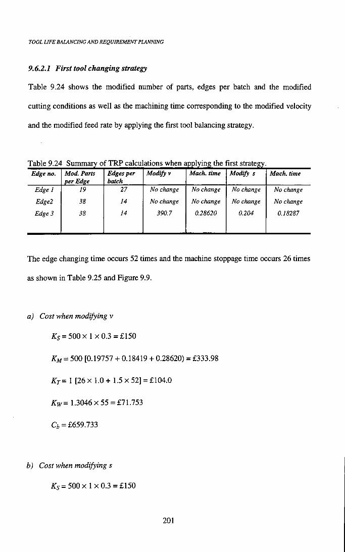
TOOL LIFE BALANCING AND REQUIREMENT PLANNING
9.6.2.1 First tool changing strategy
Table 9.24 shows the modified number of parts, edges per batch and the modified
cutting conditions as well as the machining time corresponding to the modified velocity
and the modified feed rate by applying the first tool balancing strategy.
Table 9.2- i Summary of TRP calcu ations when applying the i irst strategy. Edge no. Mod. Parts
per Edge Edges per batch
Modify V Mach. time Modify s Mach. time
Edge 1
Edge2
Edge 3
19
38
38
27
14
14
No change
No change
390.7
No change
No change
0.28620
No change
No change
0.204
No change
No change
0.18287
The edge changing time occurs 52 times and the machine stoppage time occurs 26 times
as shown in Table 9.25 and Figure 9.9.
a) Cost when modifying v
is:5 = 500x 1 x 0 . 3 = £ 1 5 0
KM = 500 [0.19757 + 0.18419 + 0.28620) = £333.98
KT= 1 [26 X 1.0+ 1.5x52] = £104.0
Kw= 1.3046x55 = £71.753
Ct = £659.733
b) Cost when modifying s
Ks = 500x 1 X 0.3 =£150
201
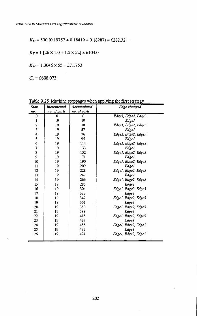
TOOL UFE BALANCING AND REQUIREMENT PLANNING
KM = 500 [0.19757 + 0.18419 + 0.18287) = £282.32
KT= 1 [26 X 1.0+ 1.5x52] = £104.0
Kw= 1.3046x55 = £71.753
Cb = £608.073
Table 9.25 Machine stoppages when applying the first strategy Stop Incremental Accumulated Edge changed no. no. o f parts no. of parts
0 0 0 Edgel, Edge2, EdgeS 1 19 19 Edgel 2 19 38 Edgel, Edge2, EdgeS 3 19 57 Edgel 4 19 76 Edgel, Edge2, EdgeS 5 19 95 Edgel 6 19 114 Edgel, Edgel, EdgeS 7 19 133 Edgel 8 19 152 Edgel, Edgel, EdgeS 9 19 171 Edgel 10 19 190 Edgel, Edgel, EdgeS 11 19 209 Edgel 12 19 228 Edgel, Edgel, EdgeS 13 19 247 Edgel 14 19 266 Edgel, Edgel, EdgeS 15 19 285 Edgel 16 19 304 Edgel, Edgel, EdgeS 17 19 323 Edgel 18 19 342 Edgel, Edgel, EdgeS 19 19 361 Edgel 20 19 380 Edgel, Edgel, EdgeS 21 19 399 Edgel 22 19 418 Edgel, Edgel, EdgeS 23 19 437 Edgel 24 19 456 Edgel, Edgel, EdgeS 25 19 475 Edgel 26 19 494 Edgel, Edgel, EdgeS
202
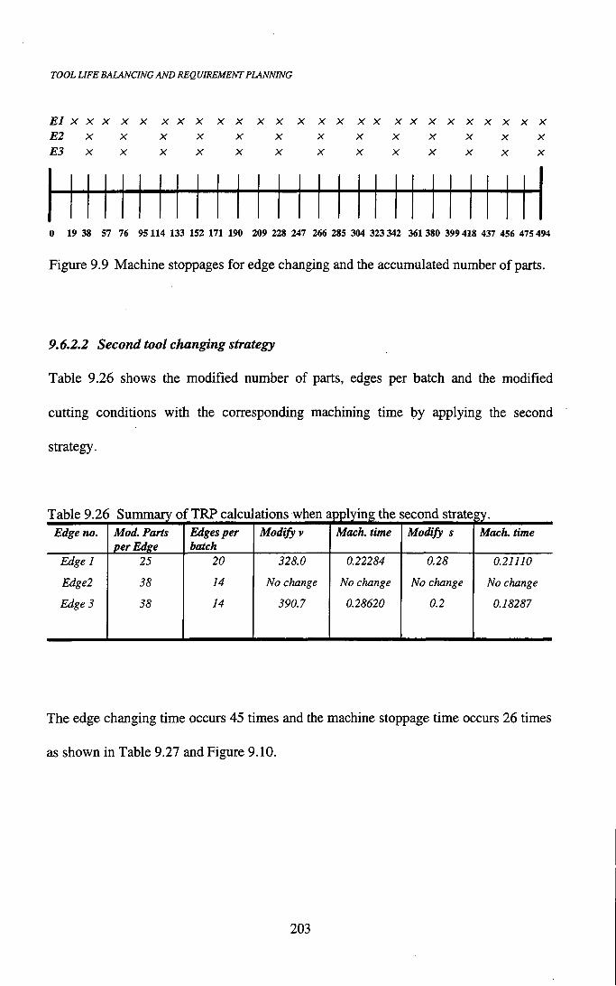
TOOL LIFE BALANCING AND REQUIREMENT PLANNING
El X X X X X X X X X X X X X X X X X X X X X X X X X X
E2 X X X X X X X X X X X X X
ES X X X X X X X X X X X X X
0 19 38 57 76 95114 133 152 171 190 209 228 247 266 285 304 323 342 361380 399 418 437 456 475 494
Figure 9.9 Machine stoppages for edge changing and the accumulated number of parts.
9.6.2.2 Second tool changing strategy
Table 9.26 shows the modified number of parts, edges per batch and the modified
cutting conditions with the corresponding machining time by applying the second
strategy.
Table 9.26 Summary of TRP calcul ations when applying the second strate gy-Edge no. Mod. Parts
per Edge Edges per batch
Modify V Mach. time Modify s Mach. time
Edge 1 25 20 328.0 0.22284 0.28 0.21110
Edge2 38 14 No change No change No change No change
Edge 3 38 14 390.7 0.28620 0.2 0.18287
The edge changing time occurs 45 times and the machine stoppage time occurs 26 times
as shown in Table 9.27 and Figure 9.10.
203
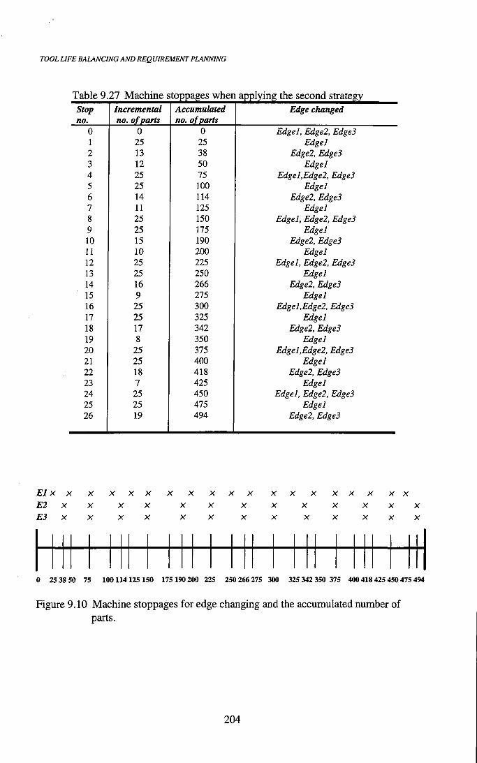
TOOL LIFE BALANCING AND REQUIREMENT PLANNING
Table 9.27 Machine stoppages when applying the second Stop Incremental Accumulated Edge changed no. no. of parts no. of parts
0 0 0 Edgel, Edgel, EdgeS 1 25 25 Edgel 2 13 38 Edgel, EdgeS 3 12 50 Edgel 4 25 75 Edgel,Edgel, EdgeS 5 25 100 Edgel 6 14 114 Edgel, EdgeS 7 11 125 Edgel 8 25 150 Edgel, Edgel, EdgeS 9 25 175 Edgel 10 15 190 Edgel, EdgeS 11 10 200 Edgel 12 25 225 Edgel, Edgel, EdgeS 13 25 250 Edgel 14 16 266 Edgel, EdgeS 15 9 275 Edgel 16 25 300 Edgel,Edgel, EdgeS 17 25 325 Edgel 18 17 342 Edgel, EdgeS 19 8 350 Edgel 20 25 375 Edgel,Edgel, EdgeS 21 25 400 Edgel 22 18 418 Edgel, EdgeS 23 7 425 Edgel 24 25 450 Edgel, Edgel, EdgeS 25 25 475 Edgel 26 19 494 Edgel, EdgeS
E l X X X X X X X X X X X X X X X X X X X
£ 2 X X X X X X x x x x x x x £ 5 X X X X X X X X X X X X X
0 25 38 50 75 100114125 150 175 190 200 225 250 266 275 300 325 342 350 375 400 418 425 450 475 494
Figure 9.10 Machine stoppages for edge changing and the accumulated number of parts.
204

TOOL UFE BALANCING AND REQUIREMENT PLANNING
a) Cost when modifying v
Ks = 500x\x0.3 = £l50
KM = 500 [0.22284 + 0.18419 + 0.28620) = £346.62
KT= 1 [26 X 1.0+ 1.5x45] = £93.5
KW= 1.3046x48 =£62.621
Ci, = £652.741
b) Cost when modifying s
Ks = 5OOx\x0.3 = £\50
KM = 500 [0.2111 + 0.18419 + 0.18287) = £289.08
KT= 1 [26 X 1.0 + 1.5 x 45] = £93.5
Kw= 1.3046x48 = £62.621
Cf, = £595.201
Finally, the system will advise the user to employ the second tool wear changing policy
with modified feed rate when machining 500 parts of component C using CNC-1000
lathe. This is because, this strategy resulted in lower cost as shown in Table 9.28.
Table 9.28 Summary of the TRP calculations for the three strategies Number of edges
Number of mach. stops
Modified parameter
Cost per batch (£)
Initial conditions 53 50 No change 668.154
First strategy 55 26 Mod. V 659.733
55 26 Mod. s 608.073
Second strategy 48 26 Mod. V 652.741
48 26 Mod. s 595.201
205

Chapter 10
CONCLUSIONS
An off-line tool life control and management system (TLC) has been developed which
will form part of an integrated tool selection system (ITS). The operation of the system
is based on metal cutting algorithms and statistical techniques such as the multiple
regression and least-squares methods. TLC is used to process tool life data from tool
catalogues as well as values found by the direct measurement of the wear land on the
flank face of carbide inserts for turning operations. TLC consists of five modules
namely, the technical planning of the cutting operation (TPO), tool life prediction (TLP),
tool life assessor (TLA), tool life management (TLM) and the tool wear balancing and
requirement planning (TRP).
The technical planning of the cutting operation module (TPO) was shown to be an
efficient, direct and fast method of selecting tools and calculating machining parameters
for turning operations by considering the process constraints such as power and
rotational speed. The logic applied by TPO to each feature (operation) for selecting
tools is based on data found in machining handbooks [MetCut Research Ass., 1980] and
has been developed by other researchers [Maropoulos 1990,1992].
206

CONCLUSIONS
In roughing and semi-roughing cuts, the depth of cut and feed rate are the most
influential parameters in making tooling decisions. The selection of tools and the
calculation of cutting conditions for finishing operations is constrained by the surface
finish requirements. The cutting conditions for all the cutting tests performed herein
were calculated using TPO module. The successful operation of this module is
demonstrated by the fact that there were no machining constraints active diuing the tests
such as vibration, power limitations and chipping problems.
The tool life prediction methods calculate the tool life values for any selected material
sub-class, insert grade and type of cut based on theoretical tool life constants which were
derived by applying multiple regression on tool manufacturers' data. Tool manufacturers
provide machinists with tables of cutting data for various component material and
carbide grade combinations. These cutting conditions result in a "notional" tool life
which is usually 15 minutes. Theoretical coefficients calculated using this data are
approximate because: (i) Tool manufacturers use general material classes and within each
class there may be several material sub-classes which exhibit different machinability
characteristics, (ii) The relationship between cutting conditions and tool life is obtained
as a result of several field tests which may not use rigorous and consistent tool failure
criteria, (iii) Additional tool life points for performing regression are obtained by
multiplying this cutting data by certain empirical factors. However, those theoretical
coefficients provide a quick starting point in the process of relating cutting conditions to
tool life. The calculated process parameters generated by TPO may change during the
execution of TLP. This is because TLP predictions are based on the optimization of
207

CONCLUSIONS
cutting data using three tool life criteria namely, user defined tool life, tool life for
minimum production cost or tool life for maximum production rate.
TLP showed good results in some tool life predictions (using theoretical coefficients)
particularly when finishing free cutting steel using TP 10 and TP20 insert grades as
shown in Table 5.2, Table 5.4 (tests 1, 2 and 4), Table 8.1 (tests 1 and 4) and Table 8.2
(test 1). The reason for this good correlation between prediction and experiment lies in
tiie fact that this specific material is a major material within this particular general class of
steels. Consequentiy, the cutting data given in tool manufacturers' catalogues relate well
to it. On the other hand, the inaccuracy of the theoretical coefficients is demonstrated by
the relative failure of TLP to accurately predict tool life in the cases shown in Table 5.4
(test 3), Table 5.6, Table 5.8, Table 8.1 (test 2, 3 and 5), Table 8.3 and Table 8.4. This
failure is linked to the difficult to machine stainless steel used in these tests. Obviously,
this material was not tiie norm used for constiiicting tiie catalogue cutting data tables.
The other observation is that tool manufacturers seriously underestimate the tool life of
carbides for difficult materials, by providing conservative cutting data and tool life
estimations. The reason behind this policy is that cuttioag data should be successfully
applied for the worst material in terms of machinability within a class.
The Crystal rule induction system was found to be very efficient and reliable in defining
the workpiece material sub-class as a result of giving the material chemical composition.
As a result of the tool life experiments, the following observations were made:
208

CONCLUSIONS
• The two most important wear types in metal cutting with carbide tools are flank wear and crater wear.
• Tool flank wear was detected by monitoring the change in power, surface finish, chip
size or the noise resulting fi-om the rubbing action of the tool and workpiece.
• The flank wear land is smaller in finishing cuts than in roughing cuts.
• The high cutting velocity performance of carbide inserts is controlled by the wear
behaviour of the flank face.
• The use of the cutting fluid reduces tool wear.
• As the cutting velocity increases, the flank wear also increases.
• With an increase in the feed rate, the flank wear also increase but not as fast as with
increasing cutting velocity.
The main reason for developing the tool life assessment module (TLA) was in order to
improve the operation of the system by creating regression curves based on real tool life
values collected from experiments. The assessor system was developed in recognition of
the fact tiiat tiie theoretical tool life coefficients provided variable accuracy of tool life
predictions. The concept of a closed loop system is used, whereby the assessor uses real
tool life information collected from processes to modify the theoretical predictions. The
experimental results obtained in the testing phases proved that the statistical treatment of
real tool life values by multiple regression and least-squares methods was successful
since tiie large majority of real tool life values shown in Figures 8.6, 8.9 and 8.12 lie
within Uie tight confidence Umits set by tiie system. Also, in the large majority of tests.
209

CONCLUSIONS
the theoretical tool life was successfully modified by TLA and was very close to the
experimental value.
Of particular interest is the appUcability in the methods for industrial environments. The
fact that there is no reliance on any sensorial feedback for collecting real tool life data is
expected to enhance the industrial application of the methods. One of the most
important aspects in the defmition of consistent tool failure criteria. Direct measurement
of the wear land is the most accurate method and has been used herein. In industry, the
collection of wear information for tools which are replaced can be achieved by using
"indirect" criteria of wear such as increased noise, vibration or power consumption. The
experimental phase showed that a limited number of observations is required for each
material, grade and type of operation combination to create stable tool life coefficients.
The immediate feedback provided by the tool life management (TLM) module is the key
indicator for measuring the success of the modified tool life data provided by the tool life
assessor. As a result from testing TLM, it was found that at least six approved points
(real tool life values) for a given workpiece material, insert grade and type of cut, are
required in order to provide the user with stabilized tool life coefficients as discussed in
Chapter 8 (Section 8.2). Again, the industrial application of methods is enhanced by the
fact that tool life predictions become highly accurate by using such a limited real tool life
information.
210

CONCLUSIONS
The tool wear balancing and requirement planning (TRP) module builds on the fact that
tool life can be accurately controlled in conjunction with cutting data. Two tool
changing methods were developed based on wear balancing theory. The two methods
are different in the ratio which controls the calculation of the number of parts each edge
can machine (i.e., the constant number of parts between cutting edge changing). As a
result of testing TRP with different examples, it was found that the system will always
advise the user to balance tool life by modifying the feed rates rather than by modifying
cutting velocities. These two strategies resulted in considerable reductions in tool
changing costs for producing a given number of components.
The overall system provides a vertical integration of tool life considerations fi"om the
initial calculation of tool life based on cutting data, to the subsequent real time
modification of tool life predictions using real tool life data and the final adjustment of
tool life and cutting data to create an optimal tool replacement strategy.
211

REFERENCES
AB Sandvik Coromant, 1985, 'Turning guide'. AB Sandvik Coromant, Sweden.
AB Sandvik Coromant, 1993, 'Coromant turning tools catalogue'. AB Sandvik
Coromant, Sweden.
Arosvski S. M.,1983, Wear sensors in the adaptive conu-ol systems of machine tools'.
Int. J. Prod. Res., 21, 347-356.
Bath M . and Sharp R.,1968, 'In-process control of lathe improves accuracy and
productivity'. Proc. 9th Int. Mach. Tools Des. and Res. Conf., 1209-1221.
Beadle B. R. and Bollinger J. G., 1971, 'Computer adaptive control of a machine tool'.
Annals of the CIRP, 19, 61-65.
Billatos S. B., Bayomi A, E., Kendall L. A. and Saundres S. C.,1986, 'A statistical wear-
model for certain tool materials with applications to machining'. Wear, 112, 257-271.
Boothroyd G., Eagle J. M. and Chishohn W. J.,1967, 'Effect of tool flank wear on the
temperatures generated during metal cutting'. Proc. 8th Int. Mach. Tools Des. and Res.
Conf., 667-680.
212

Boothroyd, G., 1989, 'Fundamentals of metal machining and machine tools'. Scripta/
McGraw-Hill, Washington, D. C , USA.
Bulm T. and Inasaki I . , 1990, 'A study on acoustic emission from the orthogonal cutting
process'. Trans. ASME, J. Eng. Ind., 112, 203-211.
Chow, J. G., and Wright, P. K., 1988, 'On line estimation of tool/chip interface
temperatures for a turning operation'. Trans. ASME, J. Eng. Ind., 110,56-64.
Chryssolouris G. and Domroese M.,1988, 'Sensor integration for tool wear estimation in
machining, sensors and controls for manufacturing'. ASME Winter Annual Meeting,
Chicago, IL, 115-123.
Citti P., Bagnoli S. and Braccesi C , 1987, 'A diagnostic method for assessing cutting
tool condition, in condition monitoring'. Pinneridge Press, Swansea, U.K., 930-939.
Colwell L. v., 1971, 'Methods for sensing rate of tool wear'. Annals of the CIRP, 19,
647-651.
Colwell L. v., 1974, Tracking tool deterioration by computer during actual machining'.
Annals of the CIRP, 23(1), 29-30.
Colwell L. V. and Mazur J. C , 1979, 'Real time computer diagnostics - a research tool
for metal cutting'. Annals of the CIRP, 28,49-52.
213
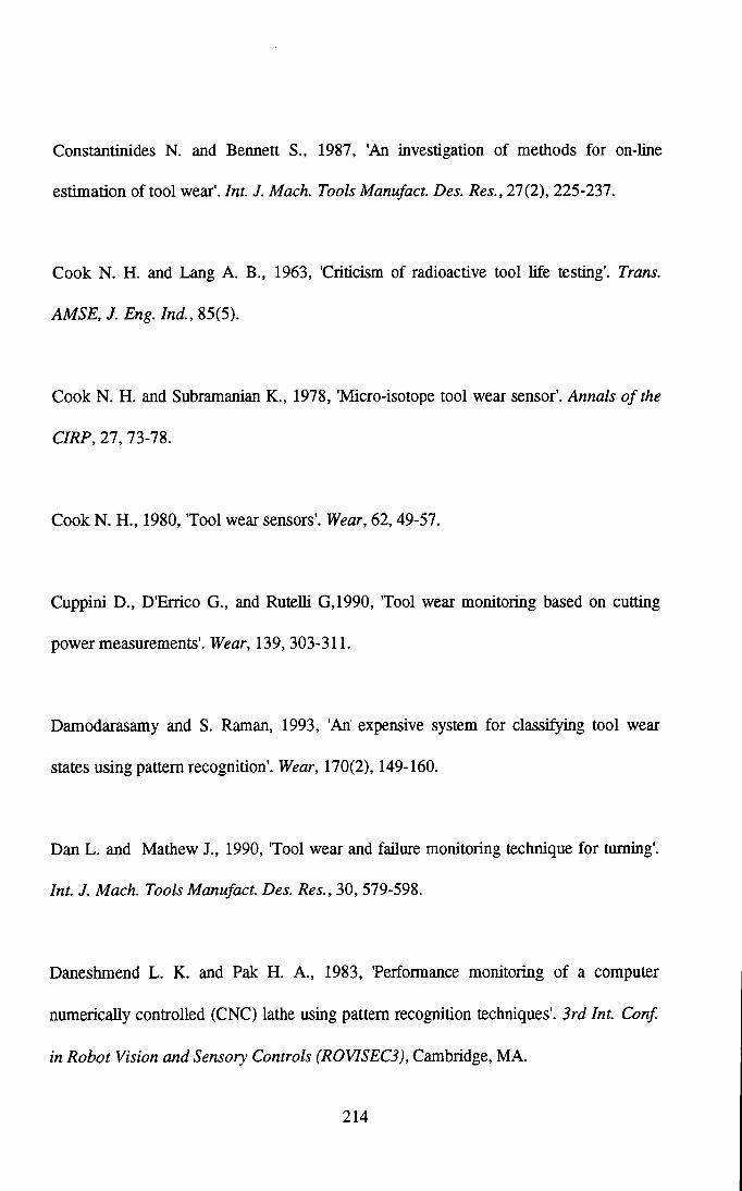
Constantinides N. and Bennett S., 1987, 'An investigation of methods for on-line
estimation of tool wear'. Int. J. Mach. Tools Manufact. Des. Res., 27(2), 225-237.
Cook N . H. and Lang A. B., 1963, 'Criticism of radioactive tool hfe testing'. Trans.
AMSE, J. Eng. Ind., 85(5).
Cook N . H. and Subramanian K., 1978, 'Micro-isotope tool wear sensor'. Annals of the
CIRP, 27,73-78.
Cook N . H., 1980, 'Tool wear sensors'. Wear, 62,49-57.
Cuppini D., D'Errico G., and RuteUi G,1990, 'Tool wear monitoring based on cutting
power measurements'. Wear, 139, 303-311.
Damodarasamy and S. Raman, 1993, 'An expensive system for classifying tool wear
states using pattern recognition'. Wear, 170(2), 149-160.
Dan L. and Matiiew J., 1990, 'Tool wear and failure monitoring technique for turning'.
Int. J. Mach. Tools Manufact. Des. Res., 30, 579-598.
Daneshmend L. K. and Pak H. A., 1983, 'Performance monitoring of a computer
numerically controlled (CNC) lathe using pattern recognition techniques'. 3rd Int. Conf
in Robot Vision and Sensory Controls (R0VISEC3), Cambridge, MA.
214
Darper N. R., and Smith, H., 1981, 'Applied Regression Analysis'. Wiely, New York.
De Filippi A. and Ippolito R., 1969, 'Adaptive control in mming: cutting forces and tool
wear relationships for PIO, P20, P30 carbides'. Annals of the. CIRP, 17, 377-385.
De FiUppi A. and Ippolito R., 1972, 'Analysis of the correlation among: cutting force
variation (vs. time)-chip formation parameters-machinabiUty'. Annals of the CIRP,
21(1).
De Garmo, E. P., Black, J. T., Kosher, R. A., 1988, 'Material and Processes in
Manufacturing'. 7th Edition, Macmillan Publishing Company.
Deutsch J, Wu S. M. and Straklowski C. M. , 1973, 'A new irregular surface measuring
system'. Int. J. Mach. Tools Des. Res., 13, 29-42.
Diei F. N . and Domfeld D. A., 1987, 'A model of tool fracture generated acoustic
emission during machining'. Trans. ASME, J. Eng. Ind., 109, 227-233.
Domfeld D., 1990, 'Neural network sensor fusion for tool condition monitoring'. Annals
of the CIRP, 39 (1), 101-105.
El Gomayel J. L. and Bregger K. D., 1986, 'On-line tool wear sensing for turning
operations'. Trans. ASME, J. Eng. Ind., 108,44-47.
215

Elbestawi M . A., Papazafiriou T. A. and Du R. X., 1991, 'In-process monitoring of tool
wear in milling using cutting force signature'. Int. J. Mach.Tools Manufact. Des. Res.,
31(1), 55-73.
Emel E. and Kaimatcy-Asibu E. J., 1988, 'Tool failure monitoring in turning by pattern
recognition analysis of AE signals'. Trans. ASME, J. Eng. Ind., 110,137-145.
Fenton, R. G., and Joseph, N. D., 1979, 'The effects of the statistical nature of tool life
on the economics of machining'. Int. J. Mach. Tools Des. Res., 19,43-50.
GaU D. A., 1969, 'Adaptive control of the abrasive cut-off operation'. Annals of the
CIRP, 17, 395-339.
Gane N. and Stephens L. W., 1983, 'Tool wear and fracture resistance of ceramic cutting
tools'. Wear, 88, 67 - 83.
Gautschi G. H. R., 1971, 'Cutting forces in machining and their routine measurement
with multi-component piezo-electric force transducers'. Proc. 12th IMTDR Conf,
Manchester, UK, 113-120.
Giusti F. and Santochi M. , 1979, 'Development of a fibre optic sensor for in process
measurement of tool flank wear'. Proc. 20th Int. Mach. Tools Des. Res. Conf, 351-360.
216

Giusti F., Santochi M . and Tanmssi G., 1984, 'A flexible tool wear sensor for NC lathes'.
Annals of the CIRP, 33, 229-232.
Groover M . P. and Kane G. E., 1971, 'A continuing study in the determination of
temperatures in metal cutting using remote thermocouples'. Trans. ASME, J. Eng. Ind.,
603-608.
Groover M . P., Karpovich R. J. and Levy E. K., 1977, A study of the relationship
between remote thermocouple temperatures and tool wear in machining'. Int. J. Prod.
Res.,25,129-Ul.
Ham I . , Schmidt A. O. and Babcock R. J., 1968, 'Experimental evaluation of tool wear
mechanisms and rate using electiron microprobe analysis'. Proc. 9th Int. Mach. Tools
Des. Res. Conf, 973-987.
Harris, C. G., Williams, J. H., and Davis A., 1989, 'Condition monitoring of machine
tools'. Int. J. Prod. Res., 27, 1445-1464.
Hoffman J., and Pedersen K. B., 1987, 'design and calibration of dynamometer of CNC
latiie'. Proc. ISthNAMRC, 1983-1988.
Hoshi T., 1981, 'In cutting tool material'. American Society for Metals, Metals Park,
Ohio, 413-426.
217
Inasaki I . and Yonetsu S., 1981, 'In-process detection of cutting tool damage by acoustic
emission measurement'. Proc. 22th Int. Mach. Tools Des. Res. Conf, 261-268.
Iwata K. and Moriwaki T., 1976, 'An application of acoustic emission measurement to
in-process sensing of tool wear'. Annals of the CIRP, 25(1), 21-26.
Jaeschke J. R., Zimmerly R. D. and Wu S. M., 1967, 'Automatic cutting tool temperature
control'. Int. Mach. Tools Des. Res., 1,465-475.
Jaing C. Y., Zhang Y. Z. and Xu H. J., 1987, 'In-process monitoring of tool wear stage
by the frequency band-energy method'. Annals of the CIRP, 36(1), 45-48.
Jeon J. U.and Kim S. W., 1988, 'Optical flank wear monitoring of cutting tools by image
processing'. Wear, 111, 207-217.
Kalpakjian S., 1992, 'Manufacturing engineering and technology'. Addison-Wesley, New
York, USA.
Kannatey-Asibu E. and Domfeld D. A., 1981, 'Quantitative relationship for acoustic
emission from orthogonal metal cutting'. Trans. ASME, J. Eng. Ind., 103, 330-340.
Kannatey-Asibu E. and Domfeld D. A, 1982, 'A study of tool wear using statistical
analysis of metal cutting acoustic emission'. Wear, 76,247-261.
218

Konig W., Langhammer K. and Schemmel H. V., 1973, 'Correlations between cutting
force components and tool wear'. Annals of the CIRP, 21(1).
Koulamas C. P., Lambert B. K., and Smith M . L., 1987, 'Optimal machining conditions
and buffer space size for tiie two-stage case'. Int. J. Prod. Res., 25, 327-336.
Kramer, B. M. , 1987, 'On tool materials for high speed machining'. Trans. ASME, J.
Eng. Ind., 109, 87-91.
Kulijanic E., 1992, 'Macro plastic deformation of cutting edge-a method for maximum
utilization of cutting tool'. Annals of the CIRP, 41(1), 151-154.
La Commare, U., Noto La Diega, S., and Passannaii. A., 1983, 'Optimal tool
replacement policies witii penalty cost for unforseen tool failure'. Int. J. Mach. Tools
Des. Res., 23, 237-243.
Lan M . S. and Domfeld D. A., 1984, 'In-process tool fracture detection'. J. Eng. Mater.
TechnoL, 106,111-118.
Langhammer K., 1976, 'Cutting forces as parameter for determining wear on carbide
lathe tools and as machinability criterion for steel'. Carbide J. Soc. Carbide Tool Engrs.
Lee L. C , 1986, 'A study of noise emission for tool failure prediction'. Int. J. Mach.
Tools Des. Res., 26, 205-215.
219

Levi, R., and Rossetto, S., 1978, 'Machining economics and tool life variation'. Trans
ASME, J. Eng. Ind., 100,318-322.
Levy E. K., Tsai C. L. and Groover M. P., 1976, 'Analytical investigation of tiie effect of
tool wear on the temperature variations in a metal cutting tool'. Trans. ASME, J. Eng.
Ind., 251-151.
Lindstrom B. and Lindberg B., 1983, "Measurements of dynamic cutting forces in tiie
cutting process, A new sensor for in-process measurement'. Proc. 24th Mach. Tools Des.
Res. Conf, 137-147.
Lister P. M. and Barrow G., 1986, 'Tool condition monitoring systems'. Proc. 26th Int.
Mach. Tools Des. Res. Conf, 271-288.
Lunde G. and Anderson P. B., 1970, 'A study of tiie wear processes of cemented carbide
cutting tools by a radioactive tiacer technique'. Int. J. Mach. Tools Des. Res., 10,79-93.
Machinnon R., Wilson G. E. and Wilkinson A. J., 1983, 'A force transducer for a turret
laflie'. Proc. 24th IMTDR Conf, Manchester, UK, 215-227.
Mackinnon R., Wilson G. E. and Wilkinson A. J., 1986, Tool condition monitoring using
multi-component force measurements'. Proc. 26th Int. Mach. Tools Des. Res. Conf, 26,
317-324.
220

Man D. and Gonseth D. R., 1993, 'A new look at carbide tool life'. Wear, 165(1), 9-7.
Maropoulos P. G., 1988, 'Automatic tool selection and balancing for CNC turning
centies'. PhD thesis, UMIST, England.
Maropoulos P. G., and Hinduja S., 1989, 'A tool-regulation and balancing system for
turning centres'. Int. J. Adv. Manuf TechnoL, 4, 207-226.
Maropoulos P. G. and Hinduja S., 1990, 'Automatic tool selection for finish turning'.
Proc. Instn. Mech. Engrs., 204 (B), 43-51.
Maropoulos P. G. and Hinduja S., 1991, 'Automatic tool selection for rough turning'. Int.
J. Prod. Res., 29 (6), 1185-1204.
Maropoulos P. G., 1992, 'Cutting tool selection: an intelligent metiiodology and its
interface with technical and planning functions'. Proc. Inst. Mech. Engrs., 206(B), 49-60.
Maropoulos P. G., 1995, 'Review of research in tooling technology, process modelling
and process planning. Part I : Tooling and process modelling'. Int. J. Computer
Integrated Manuf, 8(1), 5-12.
221

Maropoulos P. G., and Alamin B., 1995, Intelligent tool selection for machining
cylindrical components- Part 2: results from tiie testing of tiie knowledge-based module'.
Proc. Instn. Mech. Engrs., 209, 183-192.
Maropoulos P.G., and Gill P.A.T., 1995, 'Intelligent tool selection for machining
cylindrical components- Part 1: Logic of tiie knowledge based module'. Proc. Instn.
Mech. Engrs., 209, 173-182.
Martin K. F., Brandon J. A., Grosvenor B. I . and Owen A., 1986, 'A comparison of in-
process tool wear measurement metiiods in mming'. Proc. 26th Int. Mach. Tools Des.
Res. Con/, 289-296.
Martin P., Mutel B. and Drapier J. P., 1974, Influence of latiie tool wear on tiie
vibrations sustained in cutting'. Proc. 15th Int. Mach. Tools Des. Res. Conf, 251-257.
Mastuoka K., Forrest D. and Ming-Kai Tse, 1993, 'On line wear monitoring using
acoustic emission'. Wear, 162-164.
McAdams H. T. and Rosentiial P., 1961, 'Forces on a worn cutting tool'. Trans. ASME,
J. Eng. Ind., 63(4), 505-512.
Merchant M . E.and Krabacher E. J., 1951, 'Radioactive tiacers for rapid measurement of
cutting tool life'. J. App. Phy., 22(12), 1507-1508.
222

Merchant M . E., Ernst H.and Karabacher E. J., 1953, 'Radioactive cutting tools for rapid
tool-life testing'. Trans. ASME, J. Eng. Ind.
MetCut Research Associates Inc., 1980, 'Machining data handbook'. Machinability data
center, Cincinnati, Ohio.
Metiia N . K., Pandey P. C. and Chakrararti G., 1983, 'An investigation of tool wear and
vibration spectrum in milling'. Wear, 91,219-234.
Micheletti G. F., De Filippi A. and Ippolito R., 1968, 'Tool wear and cutting forces in
steel turning'. Annals of the CIRP, 16, 353-360.
Micheletti, G. F., Koenig, W., and Victor, H. R., 1976, I n process tool wear sensors for
cutting operations. Annals of the CIRP, 25 (2), 483-496.
Mills B., and Redford A. H., 1983, 'Machinability of engineering materials'. Applied
Science Publishers. England.
Moore D. S. and McCabe G. P., 1993, 'Introduction to tiie practice of statistics'. W. H.
Freeman and Company. USA.
Moriwaki T., 1984, 'Sensing and predicting of cutting tool failure'. Jpn. Soc. Precis.
Eng., 18, 90-96.
223

Moriwaki T. and Tobito M. , 1990, 'A new approach to automatic detection of life of
coated tool based on acoustic emission measurement'. Trans. ASME, J. Eng. Ind., Ill,
212-218.
Nagazaka K., and Hashimoto F., 1982, 'The estabhshment of a tool life equation
condidering the amount of tool wear'. Wear, 81, 21-31.
Naik S. K and Suh N . P, 1975, The investigation of the enhancement mechanisms of
oxide tireatinent on cemented carbide tools'. Trans. ASME, J. Eng. Ind., 97,112-
Novak A. and Ossbahr G., 1986, 'reliability of the cutting force monitoring in FMS-
instalations'. Proc. 26th Int. Mach. Tools Des. Res. Conf, 325-329.
Okushima K. and Moriwaki T., 1980, 'Detection for cutting tool fracture by acoustic
emission measurement'. Annals of the CIRP, 19, 35-40.
Olberts D. R., 1959, 'A study of the effect of tool flank wear on tool-chip interface
temperatures'. Trans. ASME, J. Eng. Ind., 152-158.
Pandit S. M. , 1978, 'Data dependent systems approach to stochastic tool life and
reUability'. Trans. ASME, J. Eng. Ind., 100, 318-322.
Pandit S. M. and Kashou S., 1982, 'A data dependent systems stiategy of on-line tool
wear sensing'. Trans. ASME, J. Eng. Ind., 104, 217-223.
224

Pandit S. M . and Kashou S., 1983, 'Variation in friction coefficient with tool wear'.
Wear, 84, 65-79.
Pederson K. B., 1988, 'A computer vision system for wear measurement of cutting tools'.
3rd Int. Conf. on Computer-aided Prod. Eng., All-ATI.
Pekelharing A. J., 1980, 'Cutting tool damage in interrupted cutting'. Wear, 62, 37.
Peklenik J., Seljak Z., Lenskovar P. and Justin B., 1973, 'Contiibution to the on-line
identification of tiie cuti;ing process'. Annals of the CIRP, 22,43-44.
Powell J. W., Kline W. A., Cosic J. E., Mayer J. E., and Herko F. M. , 1985, 'Cutting
tool sensors'. Carbide Tool J., 12-17.
Rao I . V. and Lai G. K., 1977, 'Tool life at high cutting speeds'. Int. J. Mach. Tools Des.
Res., 17, 235-243.
Ravindra H. V., Srinivasa Y. G. and Krishnamurthy R., 1993, Tvlodelling of tool wear
based on cutting forces in turning'. Wear, 169(1), 25-32.
Redford A. H., 1980, The effect on cutting tool wear of various types of chip control
device'. Annals of the CIRP, 29, 67.
225

Rutteli G. and Cuppini D., 1988, 'Development of wear sensor for tool management
system'. / . Eng. Mater. TechnoL, 110, 59-62.
Sadat A.B. and Raman S., 1987, 'Detection of tool flank wear using acoustic sugnature
analysis'. Wear, 115, 265-272.
Sade et al. T., 1972, 'In-process measurement for A/C of machines'. Jpn. Soc. Precis.
Eng.,3mO), 788-795.
Sata T. and Matsushima K., 1974, 'On-line control of the cutting state by pattern
recognition technique'. Anna/s of the CIRP, 23,151-152.
Sata T., Matsushima K. and Kawabata T., 1979, "Recognition and control of the
morphology of tool failure'. Annals of the CIRP, 28,43-47.
Seco Tools AB, 1993, 'Seco turning tools catalogue'. Seco Tools AB, Sweden.
Sekhon, G. S., 1983,' A simulation model of machining economics incorporating
stochastic variability of work and tool properties'. Int. J. Mach. Tools Des. Res., 23, 61-
69.
Shaw M . C , Smith P. A., and Cook N. H., 1961, 'Free machining steel: 1- Tool life
characteristic of resulfurized steel'. Trans. ASME. J. Eng. Ind., 83(2), 163-193.
226
Sheikh, A. K., Kendall, A., and Pandit, S. M. , 1980, 'Probabilistic optimization of
multitool machining operations'. Tran. ASME, J. Eng. Ind., 102, 239-246
Shumsherudin A. and Lawrence J. C , 1984, 'In-process prediction of milling tool wear'.
Proc. 24th Int. Mach. Tools Des. Res. Conf, MacmiQan, Birmingham, 201-214.
Singh J., and Khare M. K., 1983, 'Machining ratio as a basis for tool life assessment'.
Wear, 88, 145-154.
Society of Automative Engineers, 1981, 'SAE handbook'. Society of Automative
Engineers Inc.
Soderberg S., Vingsbo O., Loryd B. and Fredriksson B., 1981, 'Wear and wear
mechanisms during power hackswing'. Met. Corr. Ind., 57,169.
Soderberg S., Ahman L. and Svenzon M, 1983, 'A metallurgical study of die wear of
handsaw blades'. Wear, 85, 11.
Solaja V. and Vukelja D., 1973, Identification of tool wear rate by temperatiire
variation'. Anna/s of the CIRP, 22(1), 117-119.
Spirgeon D. and Slater R. A. C , 1974, 'In-process indication of surface roughness using
a fibre-optics transducer' Proc. 15th Int. Mach. Tools Des. Res. Conf., 339-347.
227
Stoferele T. H. and Bellmann B., 1975, 'Continuous measuring of flank wear'. Proc. 16th
Int. Mach. Tools Des. Res. Con/, 573-578.
Suh N . P., 1977, 'Coated carbides-past, present and future'. Carbide J., 9, 3-9.
Suh N . P., 1980, 'New theories of wear and their implication for tool life'. Wear, 62, 1-
20.
Suzuki H. and Weinamann K. J., 1985, 'An on-hne tool wear sensor for straight turning
operations'. Trans. ASME, J. Eng. Ind., 107,397-399.
Sweailem M . R., 1980, 'Experimental analysis of the correlation between cutting force
variation and nose wear in cutting operations'. Wear, 64, 281-289.
Takeyama H., Doi Y., Mitsuoka T. and Sekiguchi H., 1967, 'Sensors of tool hfe for
optimization of machining'. Proc. 8th Int.Mach. Tools Des. Res. Conf, New York, 191-
208.
Takeyama H., Sekiguchi H. and Takada K., 1970, 'One approach for optimizing control
in metal cutting'. Annals of the CIRP, 19, 345-351.
Takeyama H., Sekiguchi H., Murata R. and Mastsuzaki H., 1976, 'In-process detection
of surface roughness in machining'. Annals of the CIRP, 25,467-471.
228

Taylor, F. W., 1907, 'On tiie art of cutting metals'. Trans, ASME, 28, 31-43.
Teshima T., Shibasaka T., Takuma M., and Yamamoto A., 1993, 'Estimation of cutting
tool life by processing the tool image data with neural network'. Annals of the CIRP, 42,
59-62.
Teti R., 1989, 'Tool wear monitoring through acoustic emission'. Annals of the CIRP,
38(1) 99-102.
Tipnis V. A., 1980, 'Cutting tool wear'. Wear Control Handbook, ASME, New York,
891.
Tlusty J. and Andrews G. C , 1983, 'A critical review of sensors for unmanned
machining'. of the CIRP, 32(2), 563-572.
Tonshoff H. K., Wulfsberg J. B., Kals H. J. J, Konig W. and vanLuttervelt C. A., 1988,
'Developments and tiends in monitoring and control of machining processes'. Annals of
the CIRP, 37,611-622.
Trent E. M. , 1959, 'Tool wear and machinability'. J. Inst. Prod Engrs., 38(3), 105-130.
Trent E. M. , 1991, 'Metal Cutting'. Butterwortiis, London, UK.
229

Turkovich B. F. and Kramer B. M. , 1986, 'A comprehensive tool wear model'. Annals of
the CIRP, 35, 67-70.
Uehara K., 1972, 'On the measurement of crater wear of carbide cutting tools'. Annals of
the CIRP, 21(1), 31-32.
Uehara K., 1973, 'New attempts for short time tool life testing'. Annals of the CIRP,
22(1), 23-24.
Uehara K., Kumagai S., Mitsui H. and Takeyama H., 1974, 'Relationship between the
size of wear particles and the mechanism of tool wear in metal cutting'. Annals of the
CIRP, 23,13-14.
Uehara K., 1975, 'Characteristics of tool wear based on the volume of flank and crater
wear-a proposal on measurement of tool life'. Annals of the CIRP, 24, 59-64.
Uehara K., Kiyosawa F. and Takeshita H., 1979, 'Automatic tool wear monitoring in NC
turning". Annals of the CIRP, 28, 39-42.
Ueno S., 1972, 'In-process measurement in Europe and U.S.'. Jpn. Soc. Precis. Eng., 10,
803-807.
Wager J. G., Barash M. M., 1971, 'Study of distribution of the life of HSS tools'. Tran.
ASME, J. Eng. Ind., 91,1044-1050.
230
Wegst C. W., 1992, 'Stahlschlussel Herausgabe und Vertrieb'. Verlag Stahlschussel
Wegst GMBH.
Weller E. J., Schrier H. M. and Weichbrodt B., 1969, "What sound can be expected from
a worn tool ?'. Trans. ASME, J. Eng. Ind., 91, 525-534.
Wiatt J. G., 1963, 'Automatic in-process machine conti-ol gaging'. Trans. ASME, 17.
Wilkinson A. J., 1971, 'Constriction-resistance concept applied to wear measurement of
metal-cutting tools'. Proc. Ins. Elect. Eng., 118 (2).
Wilson G. F. and McHenry W. D., 1965, 'Study of tiie radiometric metiiod and use of the
liquid scintillation for tool wear detemination'. Trans. ASME., J. Eng. Ind., 5-9.
Wonnacott T. H., and Wannacott R. J., 1990, 'Introductory Statistics'. John Wiely and
Sons, Inc., Canada.
Yamazaki K., Yamada A., Sawai S. and Takeyama H., 1974, 'A study on adaptive
conti-ol in an NC milhng machine'. Annals of the CIRP, 23(1), 153-154.
Yingxue Y., Zhejun Y. and Haicho L., 1988, 'A new method for computer-aided
monitoring of tool wear and breakage'. 4th Int. Conf Computer-aided Prod. Eng., Univ
of Edinbrough, 455-461.
231

Zakaria A. A. and El Gomayel J. I . , 1975, 'On the reUability of the cutting temperature
for monitoring tool wear'. Int. J. Mach. Tools Des. Res., 15,195-208.
232

Appendix I. t distribution critical values
d.o.f Tail probability p (to.025)
1 12.710 2 4.303 3 3.182 4 2.776 5 2.571 6 2.447 7 2.365 8 2.306 9 '2.262 10 2.228 11 2.201 12 2.179 13 2.160 14 2.145 15 2.131 16 2.120 17 2.110 18 2.101 19 2.093 20 2.086 21 2.080 22 2.074 23 2.069 24 2.064 25 2.060 26 2.056 27 2.052 28 2.048 29 2.045 30 2.042 40 2.021 50 2.009 60 2.000 80 1.990 100 1.984 120 1.980
1000 1.962 oo 1.960
Critical point. For example: ^.025 leaves .025 probability in the tail.
233

Material Material Feed rate Finishing Medium Roughing group sub-group Roughing
s (mm/r) V (m/min) V (m/min) V (m/min) 0.1 490
1 0.2 4 8 0
0.3 455 4 3 0 390
0.4 380 345
0.1 415
2 0.2 405
0.3 385 365 330
0.4 320 290
0.1 355
3 0.2 345
0.3 330 310 280
0.4 275 245
0.1 295
Steel 4 0.2 285
Material 0.3
0.4
270 255
225
230
205
0.1 250
5 0.2 240
0.3 230 215 195
0.4 190 170
0.1 225
6 0.2
0.3
0.4
220
205 195
175
0.1 175
7 0.2
0.3
0.4
170
165 155
135
0.1 280
12 0.2 290
0.3 260 245 220
0.4 215 195
0.1 225
Cast 13 0.2 220
Iron 0.3 0.4
205 195
175
175
155
0.1 200
14 0.2
0.3
0.4
190
180 170
150
234
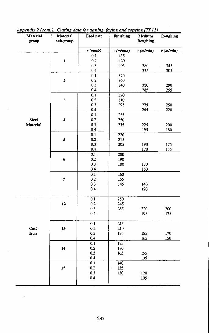
Appendix 2 (cont.). Cutting data for turning, facing and copying (TP 15) Material
group Material
sub-group Feed rate
s {mmlr)
Finishing Medium Roughing Roughing
V (m/min) v (m/min) v (m/min)
Steel Material
Cast Iron
12
13
14
15
0.1
0.2
0.3
0.4
0.1 0.2 0.3 0.4
0.1
0.2
0.3
0.4
0.1
0.2
0.3
0.4
0.1
0.2
0.3
0.4
0.1
0.2
0.3
0.4
0.1
0.2
0.3
0.4
"oT 0.2
0.3
0.4
~oT 0.2
0.3
0.4
0.1
0.2
0.3
0.4
0.1
0.2
0.3
0.4
435
4 2 0
405
370
360
340
320
310
295
255
250
235
220
215
205
"200" 190
180
160
155
145
250
245
235
215
210
195
TTT 170
165
140
135
130
380
335
320
285
275
245
225
195
190
170
170
150
140
120
220
195
185
165
155
135
120
105
345
305
290
255
250
220
200
180
175
155
200
175
170
150
235

Material Material Feed rate Finishing Medium Roughing group sub-group Roughing
s (mm/r) V (m/min) V (m/min) V (m/min) 0.1 405
1 0.2 395
0.3 375 355 320
0.4 315 285
0.1 350
2 0.2 340
0.3 325 305 280
0.4 270 245
0.1 ' 305
3 0.2 295
0.3 280 265 240
0.4 235 210
0.1 250
Steel 4 0.2 240
Material 0.3 230 215 195
0.4 190 170
0.1 220
5 0.2 215
0.3 205 190 175
0.4 170 155
0.1 190
6 0.2 180
0.3 175 165 150
0.4 145 130
0.1 155
7 0.2 150
0.3 145 135 125
0.4 120 110
0.1 155
8 0.2 150
0.3 145 135 125
Stainless 0.4 120 110
Steel 0.1 175
9 0.2 170
0.3 165 155
0.4 135
236

Material Material Feed rate Finishing Medium Roughing group sub-group Roughing
s (mm/r) V (m/min) V (m/min) V (m/min) 0.1 235
12 0.2 230
0.3 215 205 185 0.4 180 165
0.1 190
13 0.2 185
0.3 175 165 150 0.4 145 130
0.1 165
Cast 14 0.2 160
Iron 0.3 150 140 130 0.4 125 115
0.1 130
15 0.2 125
0.3 120 110 100
0.4 100 90
0.1 115
16 0.2 115
0.3 105 100 90
0.4 90 80
237

Appendix 2 (cont.). Cutting data for turning, facing and copying (TP35) Material Material Feed rate Finishing Medium Roughing
group sub-group Roughing
s (mm/r) V (m/min) V (m/min) V (m/min) 0.1 380
1 0.2 370
0.3 350 330 300 0.4 295 265
0.1 325
2 0.2 315
0.3 300 285 255
0.4 250 225
0.1 265
3 0.2 255
0.3 245 230 205
0.4 200 185
0.1 230
Steel 4 0.2 220
Material 0.3 210 200 180 0.4 175 160
0.1 205
5 0.2 200
0.3 190 180 165
0.4 160 145
0.1 150
6 0.2 145
0.3 140 130 120
0.4 115 105
0.1 130
7 0.2 125
0.3 120 115 100
0.4 100 90
0.1 200
8 0.2 195
0.3 185 175 160
0.4 155 140
0.1 130
Stainless 9 0.2 125
Steel 0.3 120 110 100
0.4 100 9 0
0.1 95
10 0.2 95
0.3 85 80 0.4 75
238

Appendix 2 (cont. ). Cutting data for turning, facing and copying (TP301) Material Material Feed rate Finishing Medium Roughing
group sub-group Roughing group sub-group s (mm/r) V (m/min) V (m/min) V (m/min)
0.1 230
8 0.2 220
0.3 210 200 180 0.4 175 160
0.1 155
Stainless 9 0.2 150
Steel 0.3 145 135 125
0.4 120 110
0.1 115
10 0.2 115
0.3 105 100 90
0.4 90 80
Appendix 2 (cont.). Cutting data for turning, facing and copying (TXIO) Material Material Feed rate Finishing Medium Roughing
group sub-group Roughing
s (mm/r) V (m/min) V (m/min) V (m/min) 0.1 200
6 0.2 195
0.3 185 175
Steel 0.4 155
Material 0.1 160
7 0.2 155
0.3 145 140
0.4 120
0.1 250
12 0.2 245
0.3 235 220 200
0.4 195 175
0.1 215
13 0.2 210
0.3 200 185 170
0.4 165 150
0.1 175
Cast 14 0.2 170
Iron 0.3 165 155
0.4 135
0.1 145
15 0.2 140
0.3 130 125
0.4 110
0.1 130
16 0.2 125
0.3 120 110
0.4 100
239
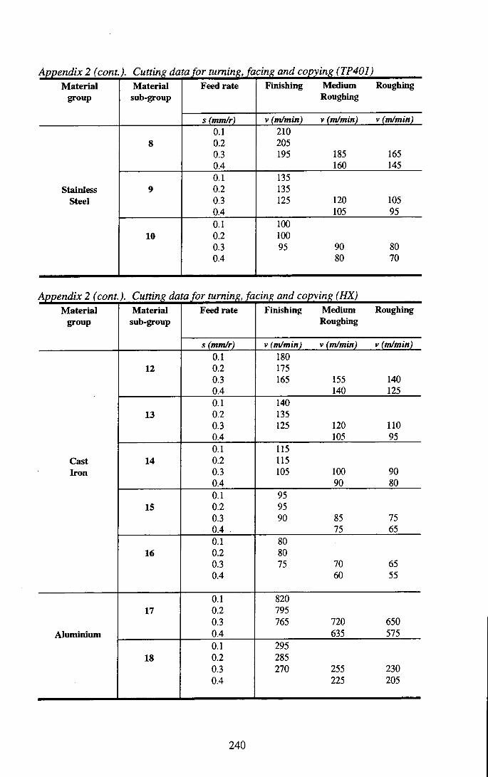
Appendix 2 (cont.). Cutting data for turning, facing and copying (TP401) Material Material Feed rate Finishing Medium Roughing
group sub-group Roughing
s (mm/r) V (m/min) V (m/min) V (m/min) 0.1 210
8 0.2 205
0.3 195 185 165
0.4 160 145
0.1 135
Stainless 9 0.2 135
Steel 0.3 125 120 105
0.4 105 95
0.1 100
10 0.2 100
0.3 95 90 80
0.4 80 70
Appendix 2 (cont. ). Cutting data for turning, facing and copying (HX) Material Material Feed rate Finishing Medium Roughing
group sub-group Roughing
s (mm/r) V (m/min) V (m/min) V (m/min) 0.1 180
12 0.2 175
0.3 165 155 140
0.4 140 125
0.1 140
13 0.2 135
0.3 125 120 110
0.4 105 95
0.1 115
Cast 14 0.2 115
Iron 0.3 105 100 90
0.4 90 80
0.1 95
15 0.2 95
0.3 90 85 75
0.4 75 65
0.1 80
16 0.2 80
0.3 75 70 65
0.4 60 55
0.1 820
17 0.2 795
0.3 765 720 650
Aluminium 0.4 635 575
0.1 295
18 0.2 285
0.3 270 255 230
0.4 225 205
240
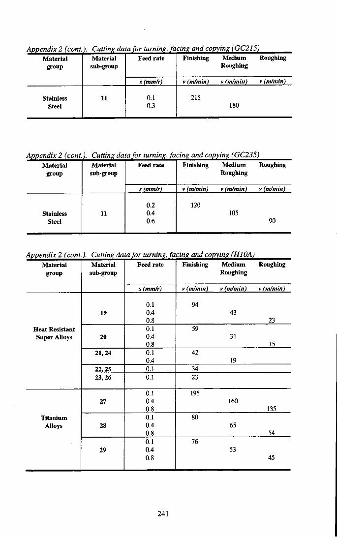
Appendix 2 (cont.). Cutting data for turning, facing and copying (GC215) Material
group Material
sub-group Feed rate Finishing Medium
Roughing Roughing
s (mm/r) V (m/min) V (m/min) V (m/min)
Stainless Steel
11 0.1 0.3
215 180
Appendix 2 (cont.). Cutting data for turning, facing and copying (GC235) Material
group Material
sub-group Feed rate Finishing Medium
Roughing Roughing
s (mm/r) V (m/min) V (m/min) V (m/min)
Stainless Steel
11 0.2 0.4 0.6
120 105
90
Appendix 2 (cont. ). Cutting data for turning, facing and copying (HI OA) Material
group Material sub-group
Feed rate Finishing Medium Roughing
Roughing
s (mm/r) V (m/min) V (m/min) V (m/min)
19 0.1 0.4 0.8
94 43
23 Heat Resistant Super Alloys 20
0.1 0.4 0.8
59 31
15 21,24 0.1
0.4 42
19 22,25 0.1 34 23,26 0.1 23
27 0.1 0.4 0.8
195 160
135 Titanium
Alloys 28 0.1 0.4 0.8
80 65
54
29 0.1 0.4 0.8
76 53
45
241

Appendix 2 (cont.). Cutting data for turning, facing and copying (GC425) Material
group Material sub-group
Feed rate Finishing Medium Roughing
Roughing
s (mm/r) V (m/min) V (m/min) V (m/min)
Stainless Steel
11 0.2 0.4 0.6
200 165
120
Appendix 2 (cont.). Cutting data for turning, facing and copying (GC435) Material
group Material sub-group
Feed rate Finishing Medium Roughing
Roughing
s (mm/r) V (m/min) V (m/min) V (m/min)
Stainless Steel
11 0.2 0.4 0.6
190 165
100
Appendix 2 (cont.). Cutting data for turning, facing and copying (HIOF) Material
group Material sub-group
Feed rate Finishing Medium Roughing
Roughing
s (mm/r) V (m/min) V (m/min) V (m/min)
19 0.3 0.6 1.2
45 27
12 Heat Resistant Super Alloys
20 0.3 0.6
30 19
21,24 0.3 17 22,25 0.3 10 23,26 0.3 10
27 0.3 0.6 1.2
135 112
95 Titanium
AUoys 28 0.3 0.6 1.2
55 45
36
29 0.3 0.6 1.2
48 42
34
242

Appendix 2 (cont.). Cutting data for turning, facing and copying (HIP) Material
group Material
sub-group Feed rate Finishing Medium
Roughing Roughing
s (mm/r) V (m/min) V (m/min) V (m/min)
30 0.1 0.3 0.5
600 430
310 Bronze-Brass
Alloys 31 0.1 0.3 0.5
395 330
275
32 0.1 0.3 0.5
285 215
165
243
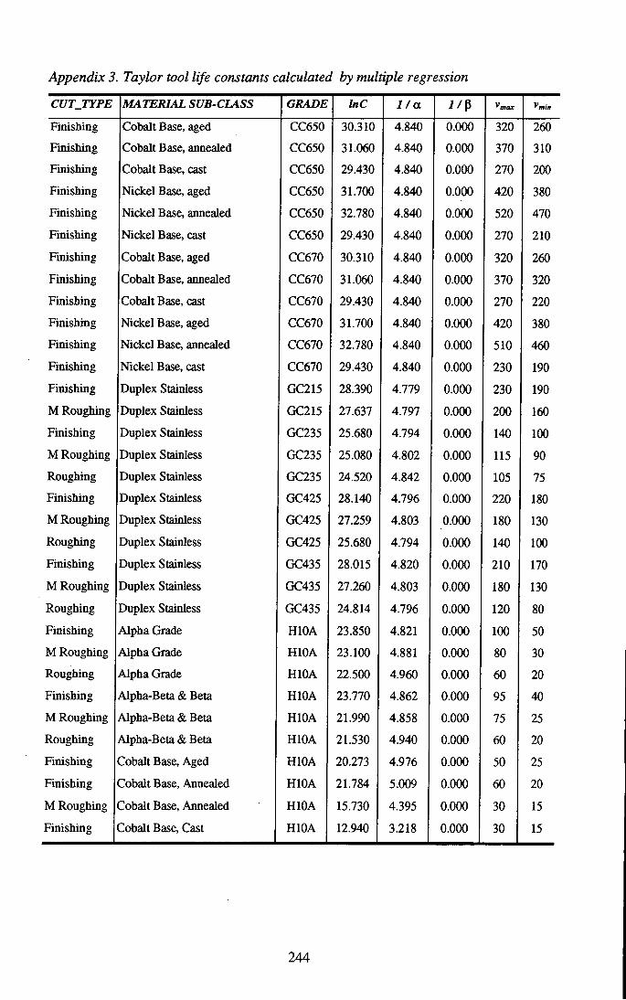
Appendix 3. Taylor tool life constants calculated by multiple regression
CUTJTYPE MATERIAL SUB-CLASS GRADE InC 1/a. 7 / p ^max
Finishing Cobalt Base, aged CC650 30.310 4.840 0.000 320 260
Finishing Cobalt Base, annealed CC650 31.060 4.840 0.000 370 310
Finishing Cobalt Base, cast CC650 29.430 4.840 0.000 270 200
Finishing Nickel Base, aged CC650 31.700 4.840 0.000 420 380
Finishing Nickel Base, annealed CC650 32.780 4.840 0.000 520 470
Finishing Nickel Base, cast CC650 29.430 4.840 0.000 270 210
Finishing Cobalt Base, aged CC670 30.310 4.840 0.000 320 260
Finishing Cobalt Base, annealed CC670 31.060 4.840 0.000 370 320
Finishing Cobalt Base, cast CC670 29.430 4.840 0.000 270 220
Finishing Nickel Base, aged CC670 31.700 4.840 0.000 420 380
Finishing Nickel Base, annealed CC670 32.780 4.840 0.000 510 460
Finishing Nickel Base, cast CC670 29.430 4.840 0.000 230 190
Finishing Duplex Stainless GC215 28.390 4.779 0.000 230 190
M Roughing Duplex Stainless GC215 27.637 4.797 0.000 200 160
Finishing Duplex Stainless GC235 25.680 4.794 0.000 140 100
M Roughing Duplex Stainless GC235 25.080 4.802 0.000 115 90
Roughing Duplex Stainless GC235 24.520 4.842 0.000 105 75
Finishing Duplex Stainless GC425 28.140 4.796 0.000 220 180
M Roughing Duplex Stainless GC425 27.259 4.803 0.000 180 130
Roughing Duplex Stainless GC425 25.680 4.794 0.000 140 100
Finishing Duplex Stainless GC435 28.015 4.820 0.000 210 170
M Roughing Duplex Stainless GC435 27.260 4.803 0.000 180 130
Roughing Duplex Stainless GC435 24.814 4.796 0.000 120 80
Finishing Alpha Grade HlOA 23.850 4.821 0.000 100 50
M Roughing Alpha Grade HlOA 23.100 4.881 0.000 80 30
Roughing Alpha Grade HlOA 22.500 4.960 0.000 60 20
Finishing Alpha-Beta & Beta HlOA 23.770 4.862 0.000 95 40
M Roughing Alpha-Beta & Beta HlOA 21.990 4.858 0.000 75 25
Roughing Alpha-Beta & Beta HlOA 21.530 4.940 0.000 60 20
Finishing Cobalt Base, Aged HlOA 20.273 4.976 0.000 50 25
Finishing Cobalt Base, Annealed HlOA 21.784 5.009 0.000 60 20
M Roughing Cobalt Base, Annealed HlOA 15.730 4.395 0.000 30 15
Finishing Cobalt Base, Cast HlOA 12.940 3.218 0.000 30 15
244

Appendix 3 (cont.) Taylor tool life constants calculated by multiple regression
CUTJTYPE MATERIAL SUB-CLASS GRADE InC 1/a ^max
Finishing Iron Base, Aged HlOA 22.096 4.754 0.000 80 30
M Roughing Iron Base, Aged HlOA 18.960 4.725 0.000 50 20
Roughing Iron Base, Aged HlOA 15.050 4.550 0.000 30 10
Finishing Iron Base, Annealed HlOA 25.003 4.906 0.000 120 80
M Roughing Iron Base, Annealed HlOA 20.350 4.692 0.000 60 25
Roughing Iron Base, Annealed HlOA 16.900 4.520 0.000 30 15
Finishing Nickel Base, Aged HlOA 20.273 4.976 0.000 50 20
Finishing Nickel Base, Annealed HlOA 21.784 5.099 0.000 60 20
M Roughing Nickel Base, Annealed HlOA 15.730 4.395 0.000 30 15
Finishing Nickel Base, Cast HlOA 12.940 3.218 0.000 30 15
Finishing Pure Titanium Alloy HlOA 28.080 4.810 0.000 250 170
M Roughing Pure Titanium Alloy HlOA 27.290 4.840 0.000 180 140
Roughing Pure Titanium Alloy HlOA 26.333 4.810 0.000 150 110
Finishing Alpha Grade HIOF 21.752 4.747 0.000 70 30
M Roughing Alpha Grade HIOF 21.530 4.945 0.000 60 20
Roughing Alpha Grde HIOF 20.240 4.890 0.000 50 15
Finishing Alpha-Beta & Beta HIOF 21.106 4.748 0.000 65 25
M Roughing Alpha-Beta & Beta HIOF 21.780 5.099 0.000 60 20
Roughing Alpha-Beta & Beta HIOF 20.270 4.980 0.000 50 15
Finishing Cobalt Base, Aged HIOF 11.584 3.792 0.000 30 10
Finishing Cobalt Base, Annealed HIOF 17.625 5.257 0.000 35 10
Finishing Cobalt Base, Cast HIOF 11.584 3.792 0.000 30 10
Finishing Iron Base, Aged HIOF 20.150 5.130 0.000 50 10
M Roughing Iron Base, Aged HIOF 15.730 4.400 0.000 30 10
Finishing Iron Base, Annealed HIOF 21.530 4.940 0.000 65 35
M Roughing Iron Base, Annealed HIOF 18.370 4.750 0.000 35 15
Roughing Iron Base, Annealed HIOF 13.440 4.330 0.000 25 10
Finishing Nickel Base, Aged HIOF 11.584 3.792 0.000 25 10
Finishing Nickel Base, Annealed HIOF 17.625 5.257 0.000 35 10
Finishing Nickel Base, Cast HIOF 11.584 3.792 0.000 25 10
Finishing Pure Titanium Alloy HIOF 26.329 4.815 0.000 150 110
M Roughing Pure Titanium Alloy HIOF 25.710 4.874 0.000 125 105
Roughing Pure Titanium Alloy HIOF 24.490 4.780 0.000 115 85
245
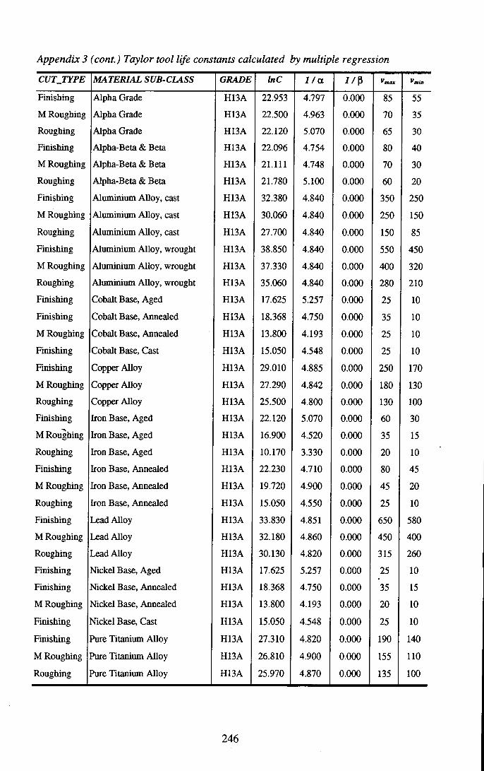
Appendix 3 (cont.) Taylor tool life constants calculated by multiple regression
CUTJTYPE MATERIAL SUB-CLASS GRADE InC 1/a ^max
Finishing Alpha Grade H13A 22.953 4.797 0.000 85 55
M Roughing Alpha Grade H13A 22.500 4.963 0.000 70 35
Roughing Alpha Grade H13A 22.120 5.070 0.000 65 30
Finishing Alpha-Beta & Beta H13A 22.096 4.754 0.000 80 40
M Roughing Alpha-Beta & Beta H13A 21.111 4.748 0.000 70 30
Roughing Alpha-Beta & Beta H13A 21.780 5.100 0.000 60 20
Finishing Aluminium Alloy, cast H13A 32.380 4.840 0.000 350 250
M Roughing Aluminium Alloy, cast H13A 30.060 4.840 0.000 250 150
Roughing Aluminium Alloy, cast H13A 27.700 4.840 0.000 150 85
Finishing Aluminium Alloy, wrought H13A 38.850 4.840 0.000 550 450
M Roughing Aluminium Alloy, wrought H13A 37.330 4.840 0.000 400 320
Roughing Aluminium Alloy, wrought H13A 35.060 4.840 0.000 280 210
Finishing Cobalt Base, Aged H13A 17.625 5.257 0.000 25 10
Finishing Cobalt Base, Annealed H13A 18.368 4.750 0.000 35 10
M Roughing Cobalt Base, Annealed H13A 13.800 4.193 0.000 25 10
Finishing Cobalt Base, Cast H13A 15.050 4.548 0.000 25 10
Finishing Copper Alloy H13A 29.010 4.885 0.000 250 170
M Roughing Copper Alloy H13A 27.290 4.842 0.000 180 130
Roughing Copper Alloy H13A 25.500 4.800 0.000 130 100
Finishing Iron Base, Aged H13A 22.120 5.070 0.000 60 30
M Roughing Iron Base, Aged H13A 16.900 4.520 0.000 35 15
Roughing Iron Base, Aged H13A 10.170 3.330 0.000 20 10
Finishing Iron Base, Annealed H13A 22.230 4.710 0.000 80 45
M Roughing Iron Base, Annealed H13A 19.720 4.900 0.000 45 20
Roughing Iron Base, Annealed H13A 15.050 4.550 0.000 25 10
Finishing Lead Alloy H13A 33.830 4.851 0.000 650 580
M Roughing Lead Alloy H13A 32.180 4.860 0.000 450 400
Roughing Lead Alloy H13A 30.130 4.820 0.000 315 260
Finishing Nickel Base, Aged H13A 17.625 5.257 0.000 25 10
Finishing Nickel Base, Annealed H13A 18.368 4.750 0.000 35 15
M Roughing Nickel Base, Annealed H13A 13.800 4.193 0.000 20 10
Finishing Nickel Base, Cast H13A 15.050 4.548 0.000 25 10
Finishing ^ e Titanium Alloy H13A 27.310 4.820 0.000 190 140
M Roughing Pure Titanium Alloy H13A 26.810 4.900 0.000 155 110
Roughing Pure Titanium Alloy H13A 25.970 4.870 0.000 135 100
246

Appendix 3 (cont.) Taylor tool life constants calculated by multiple regression
CUTJTYPE MATERIAL SUB-CLASS GRADE InC I / a J / P ^max
Finishing Red Brass and Bronze H13A 30.619 4.864 0.000 330 290
M Roughing Red Brass and Bronze H13A 29.590 4.867 0.000 270 230
Roughing Red Brass and Bronze H13A 28.080 4.810 0.000 220 175
Finishing Aluminium Alloy, cast HIP 35.240 4.840 0.000 530 480
M Roughing Aluminium Alloy, cast HIP 32.250 4.840 0.000 350 300
Roughing Aluminium Alloy, cast HIP 31.260 4.840 0.000 250 200
Finishing Aluminium Alloy, wrought HIP 40.370 4.840 0.000 830 790
M Roughing Aluminium Alloy, wrought HIP 39.370 4.840 0.000 620 580
Roughing Aluminium Alloy, wrought HIP 38.260 4.840 0.000 480 440
Finishing Copper AUloy HIP 30.149 4.853 0.000 300 260
M Roughing Copper Alloy HIP 27.680 4.640 0.000 235 200
Roughing Copper Alloy HIP 26.450 4.640 0.000 190 140
Finishing Lead Alloy HIP 33.666 4.838 0.000 620 580
M Roughing Lead Alloy HIP 32.180 4.860 0.000 450 410
Roughing Lead Alloy HIP 30.620 4.860 0.000 330 285
Finishing Red Brass and Bronze HIP 31.562 4.824 0.000 415 385
M Roughing Red Brass and Bronze HIP 30.930 4.866 0.000 345 310
Roughing Red Brass and Bronze HIP 29.820 4.820 0.000 290 255
Finishing Aluminium Alloy, cast HX 27.974 4.581 0.355 315 255
M Roughing Aluminium Alloy, cast HX 25.052 4.561 2.489 275 155
Roughing Aluminium Alloy, cast HX 24.417 4.507 2.394 250 130
Finishing Aluminium Alloy, wrought HX 32.977 4.606 0.283 835 750
M Roughing Aluminium Alloy, wrought HX 29.724 4.551 2.483 735 495
Roughing Aluminium Alloy, wrought HX 29.350 4.557 2.439 650 450
Finishing High alloy cast iron HX 22.094 4.619 0.501 90 65
M Roughing High alloy cast iron HX 15.940 3.110 0.000 80 45
Roughing High alloy cast iron HX 14.730 2.870 0.000 70 35
Finishing Low alloy cast iron HX 23.684 4.707 0.797 125 100
M Roughing Low alloy cast iron HX 20.703 4.503 2.356 100 70
Roughing Low alloy cast iron HX 20.719 4.575 2.172 90 65
Finishing Low hardness cast iron HX 25.584 4.548 0.341 180 165
M Roughing Low hardness cast iron HX 22.195 4.449 2.565 155 90
Roughing Low hardness cast iron HX 21.730 4.462 2.628 140 80
247

Appendix 3 (cont.) Taylor tool life constants calculated by multiple regression
CUTJTYPE MATERIAL SUB-CLASS GRADE InC 1/a 1 / p ^max
Finishing Medium hardness cast iron HX 24.412 4.588 0.440 140 125
M Roughing Medium hardness cast iron HX 21.256 4.534 2.688 120 80
Roughing Medium hardness cast iron HX 21.266 4.589 2.524 110 75
Finishing Medium-hard alloy cast iron HX 23.237 4.680 0.455 105 80
M Roughing Medium-hard alloy cast iron HX 18.630 3.593 0.000 100 65
Roughing Medium-hard alloy cast iron HX 16.650 3.226 0.000 90 50
Finishing Difficult tool steel TPIO 26.565 4.550 0.367 235 195
M Roughing Difficult tool steel TPIO 22.454 3.755 0.000 210 165
Finishing Free cutting steel TPIO 29.690 4.584 0.298 415 385
M Roughing Free cutting steel TPIO 23.015 3.446 0.000 365 320
Roughing Free cutting steel TPIO 22.847 3.478 0.000 330 290
Finishing Hardened steel TPIO 26.006 4.620 0.251 190 150
M Roughing Hardened steel TPIO 19.632 3.358 0.000 170 120
Finishing High carbon steel TPIO 27.974 4.581 0.355 310 260
M Roughing High carbon steel TPIO 22.243 3.531 0.000 270 210
Roughing High carbon steel TPIO 22.593 3.665 0.000 245 190
Finishing Low alloy cast iron TPIO 26.127 4.604 0.432 220 165
M Roughing Low alloy cast iron TPIO 20.811 3.531 0.000 185 140
Finishing Low hardness cast iron TPIO 25.639 4.133 0.227 290 245
M Roughing Low hardness cast iron TPIO 24.508 4.520 2.610 245 165
Roughing Low hardness cast iron TPIO 24.011 4.496 2.521 220 150
Finishing Medium hardness cast iron TPIO 26.565 4.550 0.367 235 190
M Roughing Medium hardness cast iron TPIO 23.494 4.470 2.398 195 135
Roughing Medium hardness cast iron TPIO 23.309 4.559 2.511 175 120
Finishing Normal tool steel TPIO 27.475 4.626 0.344 265 215
M Roughing Normal tool steel TPIO 21.749 3.552 0.000 225 175
Roughing Normal tool steel TPIO 20.468 3.371 0.000 210 160
Finishing Structural steel TPIO 29.042 4.594 0.290 370 310
M Roughing Structural steel TPIO 23.334 3.603 0.000 320 255
Roughing Structural steel TPIO 21.957 3.420 0.000 280 245
Finishing Very soft steel TPIO 30.331 4.562 0.292 490 455
M Roughing Very soft steel TPIO 24.211 3.550 0.000 430 380
Roughing Very soft steel TPIO 23.943 3.566 0.000 390 345
248

Appendix 3 (cont.) Taylor tool life constants calculated by multiple regression
CUTJTYPE MATERIAL SUB-CLASS GRADE InC I / a 7 / p ^max
Finishing Difficult tool steel TP15 26.127 4.604 0.432 215 170
M Roughing Difficult tool steel TP15 20.760 3.520 0.000 185 135
Finishing Free cutting steel TP15 29.020 4.572 0.331 385 325
M Roughing Free cutting steel TP15 25.861 4.514 2.468 320 220
Roughing Free cutting steel TP15 25.755 4.581 2.474 290 200
Finishing Hardened steel TP15 24.880 4.532 0.378 170 130
M Roughing Hardened steel TP15 18.310 3.160 0.000 150 100
Finishing High carbon steel TP15 27.266 4.553 0.312 270 220
M Roughing High carbon steel TP15 20.410 3.270 0.000 225 195
Roughing High carbon steel TP15 22.680 3.780 0.000 210 160
Finishing Low alloy cast iron TP15 26.006 4.620 0.251 190 150
M Roughing Low alloy cast iron TP15 19.770 3.390 0.000 170 120
Finishing Low hardness cast iron TP15 27.571 4.601 0.246 260 220
M Roughing Low hardness cast iron TP15 24.011 4.496 2.521 220 150
Roughing Low hardness cast iron TP15 23.827 4.566 2.606 200 135
Finishing Medium hardness cast iron TP15 26.019 4.489 0.374 225 180
M Roughing Medium hardness cast iron TP15 23.644 4.533 2.325 185 130
Roughing Medium hardness cast iron TP15 22.870 4.511 2.565 170 115
Finishing Medium-hard alloy cast iron TP15 24.953 4.642 0.307 150 110
M Roughing Medium-hard alloy cast iron TP15 19.120 3.430 0.000 130 95
Finishing Normal tool steel TP15 26.902 4.600 0.281 230 190
M Roughing Normal tool steel TP15 22.170 3.720 0.000 200 150
Roughing Normal tool steel TP15 21.070 3.560 0.000 190 140
Finishing Structural steel TP15 28.419 4.583 0.327 320 275
M Roughing Structural steel TP15 25.246 4.521 2.446 275 190
Roughing Structural steel TP15 25.342 4.612 2.383 250 175
Finishing Very soft steel TP15 30.142 4.625 0.294 450 390
M Roughing Very soft steel TP15 26.656 4.527 2.505 380 260
Roughing Very soft steel TP15 26.208 4.530 2.535 345 235
M Roughing Hardened steel TP20 20.530 3.642 0.000 145 105
Finishing Difficult tool steel TP20 24.064 4.084 0.016 200 155
M Roughing Difficult tool steel TP20 20.500 3.490 0.000 175 130
Roughing Difficult tool steel TP20 19.280 3.039 0.000 160 110
249

Appendix 3 (cont.) Taylor tool life constants calculated by multiple regression
CUTJFYPE MATERIAL SUB-CLASS GRADE InC 1/a i / p ^max
Finishing Free cutting stainless TP20 23.986 4.237 0.016 170 120
M Roughing Free cutting stainless TP20 20.530 3.642 0.000 150 100
Roughing Free cutting stainless TP20 19.380 3.456 0.000 135 95
Finishing Free cutting steel TP20 29.072 4.612 0.292 365 300
M Roughing Free cutting steel TP20 25.600 4.531 2.596 305 175
Roughing Free cutting steel TP20 23.987 4.309 2.503 280 160
Finishing Hardened steel TP20 23.986 4.237 0.016 170 125
Roughing Hardened steel TP20 19.380 3.456 0.000 135 100
Finishing High alloy cast iron TP20 23.684 4.707 0.797 130 95
M Roughing High alloy cast iron TP20 20.703 4.503 2.356 100 70
Roughing High alloy cast iron TP20 19.366 4.371 2.607 90 60
Finishing High carbon steel TP20 27.475 4.626 0.344 260 220
M Roughing High carbon steel TP20 23.449 4.424 2.623 215 120
Roughing High carbon steel TP20 23.397 4.504 2.616 195 110
Finishing Low alloy cast iron TP20 24.961 4.517 0.373 175 135
M Roughing Low alloy cast iron TP20 21.730 4.462 2.628 140 80
Roughing Low alloy cast iron TP20 21.900 4.562 2.578 130 75
Finishing Low hardness cast iron TP20 26.707 4.530 0.344 245 200
M Roughing Low hardness cast iron TP20 23.696 4.532 2.688 205 115
Roughing Low hardness cast iron TP20 23.110 4.498 2.660 185 105
Finishing Medium hardness cast iron TP20 26.118 4.597 0.321 200 155
M Roughing Medium hardness cast iron TP20 22.731 4.502 2.539 165 95
Roughing Medium hardness cast iron TP20 22.240 4.500 2.570 150 85
Finishing Medium-hard alloy cast iron TP20 24.546 4.639 0.328 145 105
M Roughing Medium-hard alloy cast iron TP20 20.298 4.328 2.416 110 75
Roughing Medium-hard alloy cast iron TP20 20.703 4.503 2.356 100 70
Finishing Moderately difficult stainless TP20 24.755 4.285 0.015 190 150
M Roughing Moderately difficult stainless TP20 19.770 3.388 0.000 170 120
Finishing Normal tool steel TP20 26.902 4.600 0.281 230 190
M Roughing Normal tool steel TP20 23.283 4.469 2.475 190 130
Roughing Normal tool steel TP20 23.309 4.559 2.511 175 120
Finishing Structural steel TP20 28.155 4.581 0.343 315 265
M Roughing Structural steel TP20 24.633 4.481 2.654 265 150
Roughing Structural steel TP20 24.422 4.529 2.663 240 135
250

Appendix 3 (cont.) Taylor tool life constants calculated by multiple regression
CUTJTYPE MATERIAL SUB-CLASS GRADE InC I / a J/p ^max
Finishing Very soft steel TP20 29.564 4.584 0.302 415 355
M Roughing Very soft steel TP20 25.843 4.456 2.628 355 200
Roughing Very soft steel TP20 25.331 4.450 2.646 320 180
Finishing Difficult castings stainless TP301 22.871 4.385 0.324 140 90
M Roughing Difficult castings stainless TP301 20.180 3.807 0.000 130 80
Roughing Difficult castings stainless TP301 18.950 3.619 0.000 110 70
Finishing Free cutting stainless TP301 26.896 4.602 0.373 245 200
M Roughing Free cutting stainless TP301 23.827 4.566 2.606 200 135
Roughing Free cutting stainless TP301 23.452 4.534 2.385 180 125
Finishing Moderately difficult stainless TP301 25.332 4.606 0.267 170 125
M Roughing Moderately difficult stainless TP301 20.530 3.642 0.000 150 105
Roughing Moderately difficult stainless TP301 19.380 3.456 0.000 140 100
Finishing Difficult castings stainless TP35 14.609 2.548 0.060 120 65
M Roughing Difficult castings stainless TP35 21.501 4.307 0.000 100 55
Finishing Difficult tool steel TP35 23.833 4.235 0.016 165 125
M Roughing Difficult tool steel TP35 21.900 4.562 2.578 130 75
Roughing Difficult tool steel TP35 20.843 4.475 2.839 120 65
Finishing Free cutting stainless TP35 24.524 4.131 0.015 210 165
M Roughing Free cutting stainless TP35 9.993 1.348 0.081 175 120
Roughing Free cutting stainless TP35 10.086 1.394 0.082 160 110
Finishing Free cutting steel TP35 28.597 4.601 0.327 335 390
M Roughing Free cutting steel TP35 25.012 4.495 2.666 285 160
Roughing Free cutting steel TP35 24.721 4.525 2.629 255 145
Finishing Hardened steel TP35 22.678 4.122 0.021 145 105
M Roughing Hardened steel TP35 20.927 4.479 2.595 115 65
Roughing Hardened steel TP35 20.555 4.481 2.410 100 60
Finishing High carbon steel TP35 26.896 4.602 0.373 245 200
M Roughing High carbon steel TP35 23.314 4.495 2.760 200 110
Roughing High carbon steel TP35 22.387 4.365 2.164 180 100
Finishing Moderately difficult stainless TP35 22.678 4.122 0.021 145 100
M Roughing Moderately difficult stainless TP35 20.976 3.900 0.000 130 90
Roughing Moderately difficult stainless TP35 20.180 3.810 0.000 120 70
251

Appendix 3 (cont.) Taylor tool life constants calculated by multiple regression
CUTJTYPE MATERIAL SUB-CLASS GRADE InC 1/a 2/p ^max
Finishing Normal tool steel TP35 26.522 4.599 0.302 220 170
M Roughing Normal tool steel TP35 22.387 4.365 2.614 180 100
Roughing Normal tool steel TP35 22.544 4.482 2.600 165 95
Finishing Structural steel TP35 27.693 4.607 0.318 285 225
M Roughing Structural steel TP35 24.422 4.578 2.694 230 130
Roughing Structural steel TP35 23.588 4.453 2.463 205 120
Finishing Very soft steel TP35 29.112 4.565 0.325 390 335
M Roughing Very soft steel TP35 25.363 4.434 2.666 330 185
Roughing Very soft steel TP35 25.397 4.520 2.654 300 170
Finishing Difficult castings stainless TP401 23.195 4.601 0.411 120 80
M Roughing Difficult castings stainless TP401 18.950 3.620 0.000 110 70
Roughing Difficult castings stainless TP401 17.610 3.410 0.000 100 60
Finishing Free cutting stainless TP401 26.499 4.569 0.293 220 180
M Roughing Free cutting stainless TP401 23.651 4.604 2.593 185 125
Roughing Free cutting stainless TP401 23.197 4.567 2.388 165 115
Finishing Moderately difficult stainless TP401 24.781 4.726 0.645 150 115
M Roughing Moderately difficult stainless TP401 19.120 3.430 0.000 130 95
Roughing Moderately difficult stainless TP401 20.560 3.850 0.000 115 80
Finishing Difficult tool steel TXIO 26.237 4.568 0.308 210 165
M Roughing Difficult tool steel TXIO 21.070 3.560 0.000 185 135
Finishing Hardened steel TXIO 24.880 4.532 0.378 175 125
M Roughing Hardened steel TXIO 18.310 3.160 0.000 155 105
Finishing High alloy cast iron TXIO 24.546 4.639 0.328 145 105
M Roughing High alloy cast iron TXIO 20.980 3.900 0.000 130 85
Finishing Low alloy cast iron TXIO 26.006 4.620 0.251 190 140
M Roughing Low alloy cast iron TXIO 19.770 3.390 0.000 175 115
Finishing Low hardness cast iron TXIO 27.571 4.601 0.246 265 215
M Roughing Low hardness cast iron TXIO 22.000 3.580 0.000 235 175
Roughing Low hardness cast iron TXIO 20.920 3.440 0.000 210 155
Finishing Medium hardness cast iron TXIO 26.635 4.571 0.286 225 185
M Roughing Medium hardness cast iron TXIO 21.780 3.660 0.000 195 145
Roughing Medium hardness cast iron TXIO 20.760 3.520 0.000 180 135
Finishing Medium-hard alloy cast iron TXIO 24.386 4.543 0.428 160 115
M Roughing Medium-hard alloy cast iron TXIO 19.380 3.460 0.000 140 100
252

Appendix 4 The calculation of tool life constants using multiple regression
The cutting data recommended for cutting free-cutting steel (e.g., EN8) using the TP20 insert grade are logarithmically transformed and shown in the Table below. These conditions corresponds to medium roughing (depth of cut = 3 mm) and are valid for turning, facing and copying operation.
Cutting conditions for turning ENS using TP20 grade under semi-roughing conditions
InTi Invi Insi In Ti-lnT / / I V , - - I n v In Si - Ins
2.708 5.720 -1.204 -0.795 0.434 -0.490
3.401 5.568 -1.204 -0.101 0.282 -0.490
3.807 5.485 -1.204 0.304 0.199 -0.490
4.094 5.421 -1.204 0.592 0.135 -0.490
2.708 5.598 -0.916 -0.795 0.312 -0.202
3.401 5.447 -0.916 -0.101 0.161 -0.202
3.807 5.361 -0.916 0.304 0.075 -0.202
4.094 5.298 -0.916 0.592 0.012 -0.202
2.708 5.347 -0.511 -0.795 0.061 -0.203
3.401 5.198 -0.511 -0.101 -0.088 -0.203
3.807 5.112 -0.511 0.304 -0.174 -0.203
4.094 5.043 -0.511 0.592 -0.243 -0.203
2.708 5.165 -0.223 -0.795 -0.121 -0.491
3.401 5.017 -0.223 -0.101 -0.269 -0.491
3.807 4.927 -0.223 0.304 -0.359 -0.491
4.094 4.868 -0.223 0.592 -0.418 -0.491
253

From the Table one can calculate the following:
lnf= 3.5026 Jnv=5.2S6 Ins =-0.7136
^{ lnvi-bf^)= 0.0006
^ ( /n5j- /n7)= 0.0071
2( /nVj-/;r;^)(/n7; -inT)=-0.9373
Y^ilnSi-'hTs) {inTi -h[f)= 0.000
X(/nvj-/n^)^ = 0.9465
^{inSi-hTsf =2.2519
5 {invi -Inv) {insI )] = -1.2908
Estimating equations (4.6) and (4.7).
• 0.9373 = 0.9465 ( - ^ ) + ( - \ .2908) f -^ ) (i)
0.0 = (- 1.2908) ( - ^ ) + 2.2529 ( - j ) (ii)
From equation (ii)
= 1-745 f ^ j . (iii)
substituting into equation (i)
0.9373 = 1.652 ( - ^ ) -i- (- 1.2908) ( -^ ) P P
254

4 =-2.596
Substituting into equation (iii)
4 =-4.53
From equation (4.8):
A InC = 3.5026 - (- 4.53) x 5.286 - (- 2.596) x (- 0.7136)
A InC =25.596
Equation (4.2) can be written as:
lnT = 25.596 - (- 4.53) Inv - (- 2.596) Ins
255

Appendix 5. Pictures of some indexable inserts used in the initial testing phase
Test 1 (a = 1.3 mm, s = 0.15 mm/rev, v = 415 m/min)
Test 2 (a = 1.5 mm, s = 0.1 mm/rev, v = 450 m/min)
Test 3 (a = 1.0 mm, s = 0.2 mm/rev, v = 400 m/min)
A. TPIO inserts used for finishing ENS steel (Table 5.1)
256

Appendix 5 (cont.). Pictures of some indexable inserts used in the initial testing phase
Test 2 (a = 1.1 mm, s = 0.19 mm/rev, v = 390 m/min)
Test 3 (a = 1.5 mm, s = 0.2 mm/rev, v = 395 m/min)
Test 4 (a = 0.7 mm, s = 0.23 mm/rev, v = 450 m/min)
B. TP20 inserts used for finishing EN8 steel (Table 5.3)
257
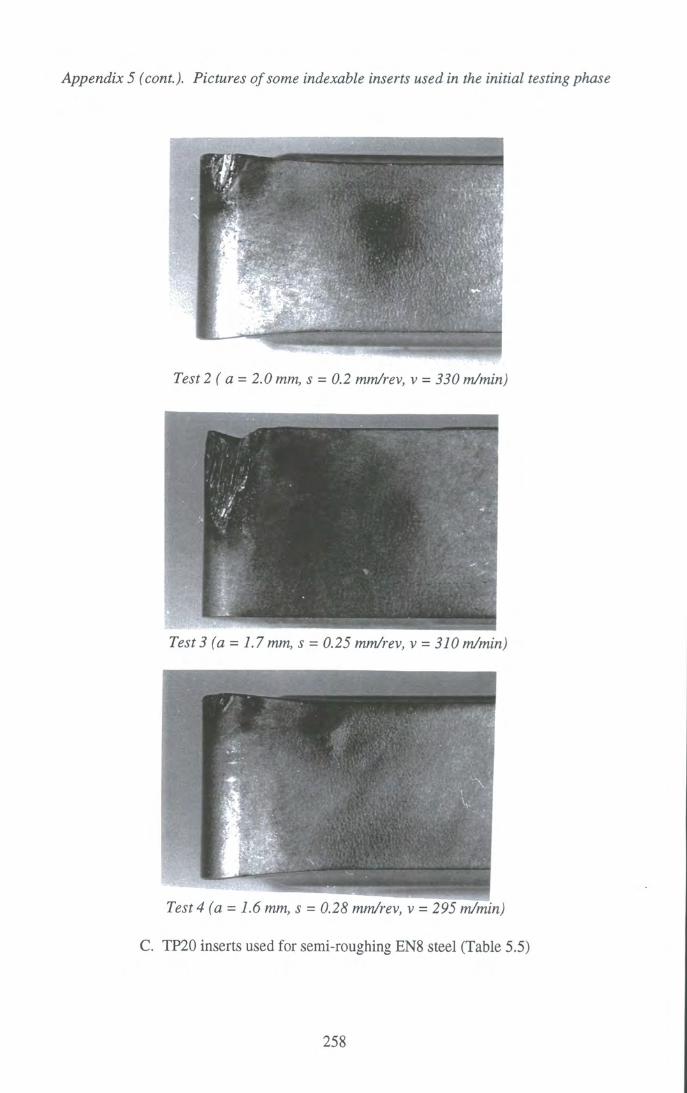
Appendix 5 (cont.). Pictures of some indexable inserts used in the initial testing phase
Test 2( a = 2.0 mm, s = 0.2 mm/rev, v = 330 m/min)
Test 3 (a = 1.7mm, s = 0.25 mm/rev, v = 310 m/min)
Test 4 (a = 1.6 mm, s = 0.28 mm/rev, v = 295 tn/min)
C. TP20 inserts used for semi-roughing ENS steel (Table 5.5)
258

Appendix 5 (cont.). Pictures of some indexable inserts used in the initial testing phase
Test 1 (a = 3.0 mm, s = 0.25 min/rev, v = 150 m/min)
Test 2 (a = 3.0 mm, s = 0.3 nun/rev, v = 125 m/min)
Test 4 (a = 3.0 nun, s = 0.4 mm/rev, v = 110 m/min)
D. TP35 inserts used for semi-roughing SS316 stainless steel (Table 5.7)
259
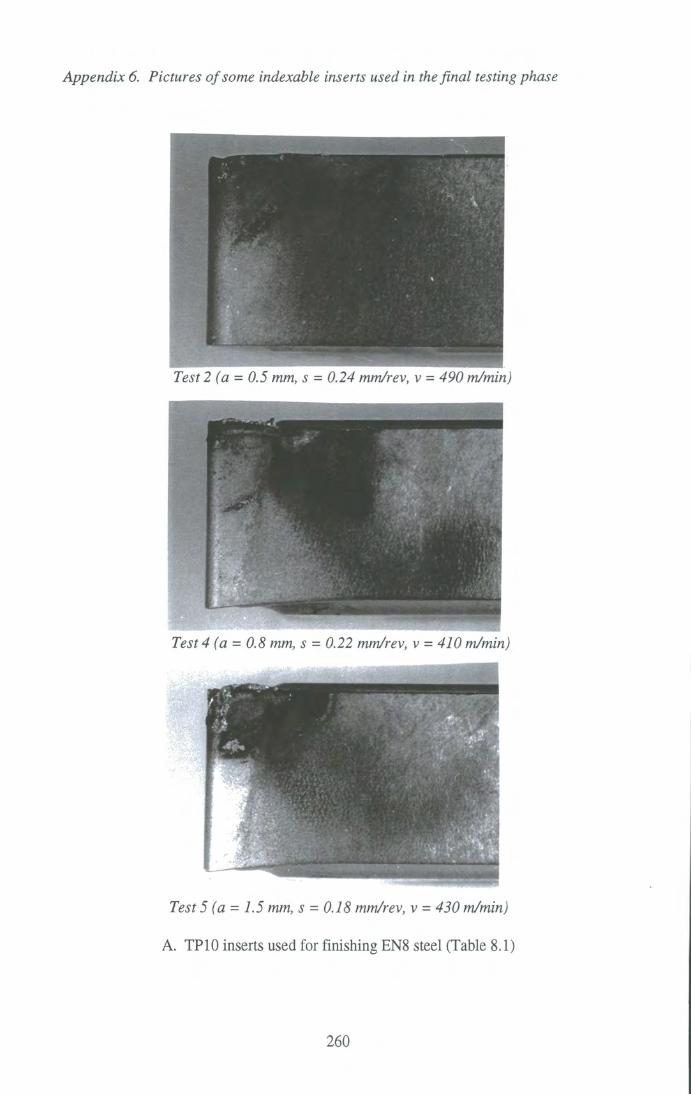
Appendix 6. Pictures of some indexable inserts used in the final testing phase
Test 2 (a = 0.5 mm, s = 0.24 mm/rev, v = 490 m/min)
Test 4 (a = 0.8 mm, s = 0.22 mm/rev, v = 410 m/min)
Test 5 (a = 1.5 mm, s = 0.18 mm/rev, v = 430 m/min)
A. TP 10 inserts used for finishing ENS steel (Table S.l)
260

Appendix 6 (cont.). Pictures of some indexable inserts used in the final testing phase
Test 1 (a = 0.5 mm, s = 0.24 mm/rev, v = 470 m/min)
Test 3 (a = 1.4 mm, s = 0.17 mm/rev, v = 360 m/min)
Test 4 (a = 0.9 mm, s = 0.21 min/rev, v = 410 m/min)
B. TP20 inserts used for finishing ENS steel (Table 8.2)
261

Appendix 6 (cont.). Pictures of some indexable inserts used in the final testing phase
Test 2 (a = 1.9 mm, s = 0.23 mm/rev, v = 320 m/min)
Test 3 (a = 1.7 mm, s = 0.26 mm/rev, v = 305 m/min)
Test 5 (a = 1.8 mm, s = 0.24 mm/rev, v = 315 m/min)
C. TP20 inserts used for semi-roughing ENS steel (Table 8.3)
262

Appendix 6 (cont.). Pictures of some indexable inserts used in the final testing phase
Test 1 (a = 3.0 mm, s = 0.3 mm/rev, v = 140 m/min)
Test 2 (a = 3.0 mm, s = 0.25 mm/rev, v = 120 m/min)
Test 3 (a = 3.0 mm, s = 0.4 mm/rev, v = 100 m/min)
D. TP35 inserts used for semi-roughing SS316 stainless steel (Table 8.4)
263