durham e-theses power conditioning unit for small …
TRANSCRIPT

Durham E-Theses
POWER CONDITIONING UNIT FOR SMALL
SCALE HYBRID PV-WIND GENERATION
SYSTEM
AHMED-MAHMOUD, ASHRAF
How to cite:
AHMED-MAHMOUD, ASHRAF (2011) POWER CONDITIONING UNIT FOR SMALL SCALE
HYBRID PV-WIND GENERATION SYSTEM, Durham theses, Durham University. Available at DurhamE-Theses Online: http://etheses.dur.ac.uk/580/
Use policy
The full-text may be used and/or reproduced, and given to third parties in any format or medium, without prior permission orcharge, for personal research or study, educational, or not-for-prot purposes provided that:
• a full bibliographic reference is made to the original source
• a link is made to the metadata record in Durham E-Theses
• the full-text is not changed in any way
The full-text must not be sold in any format or medium without the formal permission of the copyright holders.
Please consult the full Durham E-Theses policy for further details.

Academic Support Oce, Durham University, University Oce, Old Elvet, Durham DH1 3HPe-mail: [email protected] Tel: +44 0191 334 6107
http://etheses.dur.ac.uk
2

POWER CONDITIONING UNIT FOR SMALL
SCALE HYBRID PV-WIND GENERATION
SYSTEM
By
ASHRAF ABDEL HAFEEZ AHMED MAHMOUD
A Thesis presented for the degree of
Doctor of Philosophy
New and Renewable Energy Group
School of Engineering and Computing Sciences
Durham University
UK
2010

POWER CONDITIONING UNIT FOR SMALL SCALE
HYBRID PV-WIND GENERATION SYSTEM
Submitted for the degree of Doctor of Philosophy
ABSTRACT
Small-scale renewable energy systems are becoming increasingly popular due to
soaring fuel prices and due to technological advancements which reduce the cost of
manufacturing. Solar and wind energies, among other renewable energy sources, are
the most available ones globally. The hybrid photovoltaic (PV) and wind power
system has a higher capability to deliver continuous power with reduced energy
storage requirements and therefore results in better utilization of power conversion
and control equipment than either of the individual sources. Power conditioning units
(p.c.u.) for such small-scale hybrid PV-wind generation systems have been proposed
in this study. The system was connected to the grid, but it could also operate in
standalone mode if the grid was unavailable. The system contains a local controller
for every energy source and the grid inverter. Besides, it contains the supervisory
controller.
For the wind generator side, small-scale vertical axis wind turbines (VAWTs) are
attractive due to their ability to capture wind from different directions without using a
yaw. One difficulty with VAWTs is to prevent over-speeding and component over-
loading at excessive wind velocities. The proposed local controller for the wind
generator is based on the current and voltage measured on the dc side of the rectifier
connected to the permanent magnet synchronous generator (PMSG). Maximum power
point tracking (MPPT) control is provided in normal operation under the rated speed
using a dc/dc boost converter. For high wind velocities, the suggested local controller
controls the electric power in order to operate the turbine in the stall region. This high
wind velocity control strategy attenuates the stress in the system while it smoothes the
power generated. It is shown that the controller is able to stabilize the nonlinear
system using an adaptive current feedback loop. Simulation and experimental results
are presented.

Page ii
The PV generator side controller is designed to work in systems with multiple energy
sources, such as those studied in this thesis. One of the most widely used methods to
maximize the output PV power is the hill climbing technique. This study gives
guidelines for designing both the perturbation magnitude and the time interval
between consecutive perturbations for such a technique. These guidelines would
improve the maximum power point tracking efficiency. According to these guidelines,
a variable step MPPT algorithm with reduced power mode is designed and applied to
the system. The algorithm is validated by simulation and experimental results.
A single phase H-bridge inverter is proposed to supply the load and to connect the
grid. Generally, a current controller injects active power with a controlled power
factor and constant dc link voltage in the grid connected mode. However, in the
standalone mode, it injects active power with constant ac output voltage and a power
factor which depends on the load. The current controller for both modes is based on a
newly developed peak current control (p.c.c.) with selective harmonic elimination. A
design procedure has been proposed for the controller. Then, the method was
demonstrated by simulation. The problem of the dc current injection to the grid has
been investigated for such inverters. The causes of dc current injection are analyzed,
and a measurement circuit is then proposed to control the inverter for dc current
injection elimination. Characteristics of the proposed method are demonstrated, using
simulation and experimental results.
At the final stage of the study, a supervisory controller is demonstrated, which
manages the different operating states of the system during starting, grid-connected
and standalone modes. The operating states, designed for every mode, have been
defined in such a hybrid model to allow stability and smooth transition between these
states. The supervisory controller switches the system between the different modes
and states according to the availability of the utility grid, renewable energy
generators, the state of charge (SOC) of energy storage batteries, and the load. The
p.c.u. including the supervisory controller has been verified in the different modes and
states by simulation.

Page iii
Dedicated to my Father (Shikh Abdel hafeez Alsony) who passed away during the course of this work
May Allah rest his gentle soul in eternal peace
Aamen

Page iv
Declaration
The work in this thesis is based on research carried out within the New and
Renewable Energy Group, School of Engineering and Computing Sciences, Durham
University, United Kingdom. No part of this thesis has been submitted elsewhere for
any other degree or qualification and it all my own work unless referenced to the
contrary in the text.
Copyright © 2010 by Ashraf abdel hafeez Ahmed Mahmoud.
“The copyright of this thesis rests with the author. No quotations from it should be
published without the author’s prior written consent and information derived from it
should be acknowledged”.

Page v
Acknowledgements
First, I would like to thank Allah, for His mercy on me during all my life, and
praise the prophet Mohamad (peace be upon him!). I dedicate this work to my
father (Shikh Abdel hafeez Alsony-May ALLH give mercy to his soul), my mother,
my brothers (Arfat-Soliman-Ahmed), my sisters and my wife. Furthermore, I
greatly appreciate the support which I received from my supervisors, Dr. Li Ran
and Dr. Jim Bumby. Finally, I want to declare that this work was supported and
funded by the Government of Egypt (Desert Research Centre (DRC) – Cairo).

Page vi
List of publications
[1] Ahmed, L. Ran, and J. R. Bumby, “New Constant Electrical Power Soft-Stalling Control for Small-Scale VAWTs,” IEEE Transactions on Energy Conversion, vol. 25, no. 4, pp. 1125-1161, 2010.
[2] A. Ahmed, L. Ran, and J. R. Bumby, “Stalling Region Instability Compensation for Constant Power Soft Stalling Control,” 5th IET International Conference on Power Electronics, Machines and Drives (PEMD), Brighton, UK, 2010.
[3] A. Ahmed, L. Ran, and J. R. Bumby, “Sizing and Best Management of Stand Alone Hybrid PV-Wind System using logistical model,” IFAC conference on control methodologies and technology for energy efficiency, Vilamoura, Portugal (CMTEE), 2010.
[4] A. Ahmed, L. Ran, and J. R. Bumby, “Sizing and Best Management of Stand Alone Hybrid PV-Wind System using logistical model,” The First International Conference on Sustainable Power Generation and Supply (SUPERGEN), Nanjing, China, 2009.
[5] A. Ahmed, L. Ran, and J. R. Bumby, “Simulation and control of a hybrid PV-wind system,” 4th IET International Conference on Power Electronics, Machines and Drives (PEMD), York, UK, 2008.
[6] A. Ahmed, L. Ran, and J. R. Bumby, “PV Generator Control in Multi Source Renewable Energy Systems,” to be submitted soon for Journal publication.

Page vii
CONTENTS
ABSTRACT i DECLARATION iv ACKNOWLEDGEMENTS v LIST OF PUBLICATIONS vi LIST OF FIGURES x LIST OF TABLES xiii NOMENCLATURE xiv CHAPTER (1) INTRODUCTION 1
1.1 SMALL-SCALE HYBRID PV-WIND SYSTEMS 1 1.2 STUDY SYSTEM AND RESEARCH OBJECTIVES 3
1.2.1. WIND GENERATOR SIDE 4 1.2.2. PV GENERATOR SIDE 5 1.2.3. INVERTER SIDE 5 1.2.4. SUPERVISORY CONTROLLER 7
1.3. THESIS OUTLINE 7 CHAPTER (2) REVIEW OF PREVIOUS WORK 9
2.1. WIND GENERATOR CONTROL 9 2.1.1. MPPT ALGORITHMS 10 2.1.2. HIGH WIND VELOCITY CONTROL 14 2.1.3. SUMMARY AND GUIDELINES 15
2.2. PV CONTROL REVIEW 16 2.2.1. DIRECT METHODS 17 2.2.2. INDIRECT METHOD 21 2.2.3. SUMMARY AND GUIDELINES 21
2.3. INVERTER SIDE CONTROL 22 2.3.1. CURRENT CONTROL METHODS 23 2.3.2. GRID-CONNECTED CONTROL 26 2.3.3. STANDALONE MODE CONTROL 27 2.3.4. DC-ELIMINATION METHOD REVIEW 28
2.4. SUPERVISORY CONTROL METHODS REVIEW 29 2.4.1 CONVENTIONALLY-BASED METHODS 30 2.4.2. ARTIFICIAL INTELLIGENCE-BASED METHODS 31 2.4.3 SUMMARY AND GUIDELINES 32
CHAPTER (3) CONTROL ON WIND POWER SIDE 34 3.1. INTRODUCTION 34 3.2. THE PROPOSED CONTROL METHOD 35 3.3. CONSTANT POWER SOFT STALLING CONCEPT 36 3.4. SYSTEM MODELLING AND CONTROL DESIGN 39
3.4.1. SYSTEM MODELING 39 3.4.2. HIGH WIND VELOCITY STABILITY COMPENSATION 44 3.4.3. ADAPTIVE SOFT STALLING CONTROL LOOP 48
3.5. SIMULATION RESULTS 49 3.6. CONSTANT SPEED VERSUS CONSTANT POWER STALLING 54 3.7. EXPERIMENTAL VERIFICATION 56
Page viii
CHAPTER (4) CONTROL ON PV POWER SIDE 62 4.1. INTRODUCTION 62 4.2. PV GENERATOR MODEL 64 4.3. PERTURBATION PARAMETERS DESIGN 69
4.3.1. TRANSIENT ANALYSIS 69 4.3.2. DESIGN OF PERTURBATION PARAMETERS 71 4.3.3. DESIGN VERIFICATION 76 4.3.4. SUMMARIZING THE RESULTS 80
4.4. PV CONTROL ALGORITHM WITH REDUCED POWER MODE 81 4.4.1. VARIABLE STEP SIZE I.C. (V.S.I.C.) METHOD 82 4.4.2. THE REDUCED POWER MODE 86 4.4.3. THE PROPOSED V.S.I.C. METHOD VS THE P&Q ALGORITHM 88 4.4.4 DYNAMIC SIMULATION RESULTS 89
4.5. EXPERIMENTAL VERIFICATION 93 CHAPTER (5) INVERTER CONTROL 98
5.1. INTRODUCTION 98 5.2. THE PEAK CURRENT CONTROL METHOD 99
5.2.1 LCL-Filter 105 5.2.2 Selective Harmonic Elimination 107
5.3. GRID-CONNECTED CONTROL 110 5.4. STANDALONE MODE CONTROL 116 5.5. DC INJECTION ELIMINATION 120
5.5.1. THE PROPOSED CONTROL STRATEGY 120 5.5.2. CAUSES OF DC INJECTION 121 5.5.3. THE PROPOSED DC ELIMINATION TOPOLOGY 123 5.5.4. PROPOSED DC INJECTION MEASUREMENT CIRCUIT 123 5.5.5. CHOOSING MEASURING CIRCUIT COMPONENTS 124 5.5.6. CONTROLLER DESIGN 126 5.5.7. SIMULATION RESULTS 128 5.5.8. EXPERIMENTAL VERIFICATION 128
CHAPTER (6) SUPERVISORY CONTROLLER 132 6.1. INTRODUCTION 132 6.2. SYSTEM CONFIGURATION AND CONTROL 133
6.2.1. PV GENERATOR SIDE CONTROL 133 6.2.2. WIND GENERATOR SIDE CONTROL 133 6.2.3. BATTERY BANK SIDE CONTROL 134 6.2.4. INVERTER SIDE 138 6.2.5. LOAD SIDE 139
6.3. THE SUPERVISORY CONTROLLER 141 6.3.1. STARTING MODE (S0(SM)) 143 6.3.2. STANDALONE MODE 144 6.3.3. GRID-CONNECTED MODE OF OPERATION 145 6.3.4. THE SUPERVISORY CONTROLLER ALGORITHM 146
6.4. SIMULATION RESULTS 148 CHAPTER (7) CONCLUSION 158
7.1. WIND GENERATOR SIDE 158 7.2. PV GENERATOR SIDE 159 7.3. INVERTER SIDE 159 7.4. SUPERVISORY CONTROLLER 160

Page ix
7.5. THE CONTRIBUTIONS 161 7.6. FUTURE WORK 161
BIBLIOGRAPHY 162

Page x
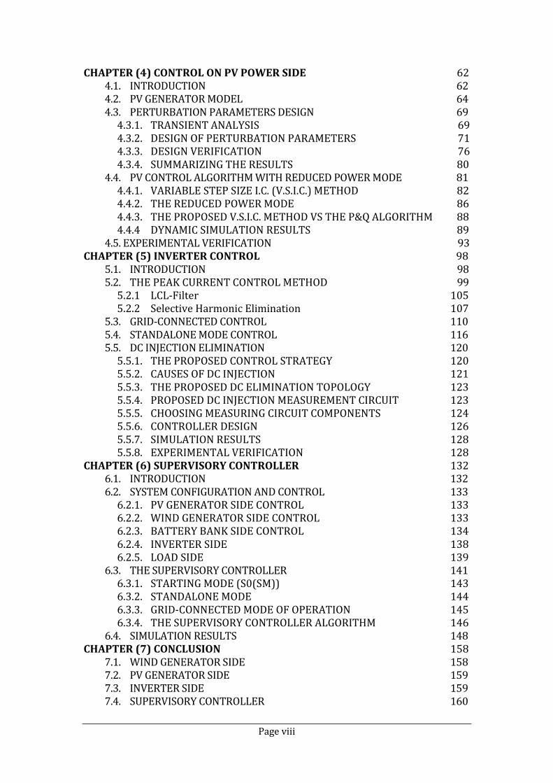
LIST OF FIGURES
Figure (1.1) A schematic for the system 4 Figure (1.2) Diagram describes the proposed research in the thesis 8 Figure (2.1) Power-rotor speed curve in constant speed soft stalling 15 Figure (2.2) A chart for the wind generator MPPT control algorithms 16 Figure (2.3) A chart shows the different PV MPPT algorithms 22 Figure (2.4) Carrier-based method with PI regulator 24 Figure (2.5) Carrier-based method with PIS regulator 24 Figure (2.6) Hysteresis-based current controller 25 Figure (3.1) Block diagram – wind turbine with PMSG and grid connection 35 Figure (3.2) Typical cp-λ curve for VAWT 37 Figure (3.3) Concept of constant power soft stalling control 38 Figure (3.4) Dc side voltage-current relationship 38 Figure (3.5) A simplified wind generator system 40 Figure (3.6) PI control algorithm 42 Figure (3.7) Stability analysis of original control algorithm 43 Figure (3.8) Control algorithm with stability compensation 44 Figure (3.9) Root locus of closed-loop system 46 Figure (3.10) First pole with inertia=8 46 Figure (3.11) Second pole with inertia=8 47 Figure (3.12) Effect of inertia on the value of Tc to stabilize the system 48 Figure (3.13) Adaptive control loop effect 49 Figure (3.14) The proposed controller 49 Figure (3.15) Simulation results with wind velocities lower than the rated values 51 Figure (3.16) Simulation results with wind velocities higher than the rated values 52 Figure (3.17) Fluctuations due to rapid wind velocity change 53 Figure (3.18) Power output: constant power stalling vs constant speed stalling 55 Figure (3.19) PMSG temperature rise with constant speed stalling and constant power stalling methods 56 Figure (3.20) Laboratory test rig 57 Figure (3.21) Arrangement of laboratory system 57 Figure (3.22) Block diagram for the wind turbine model 58 Figure (3.23) Experimental results with step changes in wind velocity 60 Figure (3.24) Experimental results with a dynamic wind velocity time-series 61 Figure (4.1) A block diagram of the proposed system 63 Figure (4.2) The solar cell model 64 Figure (4.3) PV generator characteristics for solar radiation1000 W/m2 and 300 W/m2, temperature 20oc and 40oc: (a) current (Ipv) vs. voltage (Vpv) and (b) power (Ppv) vs. voltage (Vpv) 68 Figure (4.4) Simplified circuit for the system model 70 Figure (4.5) IPV-VPV curve are Tc=20oC, s=800 W/m2 73 Figure (4.6) Root locus for the PV system according to Ipv-Vpv curve shown in figure (4.5) 73
Page xi
Figure (4.7) Absolute value of Rpv plotted against Vpv 74 Figure (4.8) Step response in ΔPpv according to: (a) operating point a, (b) operating point b, and (c) operating point c as shown in Figure (4.5) 76 Figure (4.9) Perturb and observe algorithm 77 Figure (4.10) Ppv output with different design perturbation parameters 78 Figure (4.11) The measured solar radiation (S), the duty ratio (D), the dc output voltage (Vpv), the dc output current (Ipv) and the dc output power (Ppv) for the three simulation cases 79 Figure (4.12) Duty waveforms zoom between t=5 and t=10 in Figure (4.11) 80 Figure (4.13) Data sheet design of the perturbation parameters 81 Figure (4.14) The basic idea for the V.S.I.S. method 84 Figure (4.15) δdp versus dinc 85 Figure (4.16) The proposed algorithm for V.S.I.C. method 85 Figure (4.17) Overrating levels of the PV output pwer with decreasing in temperature and increasing in solar radiation 87 Figure (4.18) The PV output power produced by the proposed V.S.I.C. algorithm compared to the P&O algorithm 88 Figure (4.19) The proposed V.S.I.C. tracking speed compared to I.C. and P&O 89 Figure (4.20) Dynamic simulation results verifying the accuracy of the proposed V.S.I.C. method in the MPPT mode of operation 91 Figure (4.21) Dynamic simulation results verifying the accuracy of the proposed V.S.I.C. method in the reduced power mode of operation 92 Figure (4.22) Laboratory test rig 94 Figure (4.23) Arrangement of laboratory system 94 Figure (4.24) Experimental results for MPPT mode of operation as the solar radiation and temperature change from (1000 W/m2 and 25 OC) TO (500 W/m2 and 40 OC) respectively 95 Figure (4.25) Proposed V.S.I.C control against fixed step I.C. 96 Figure (4.26) Experimental results for reduced power mode of operation as the solar radiation and the temperature (1000 W/m2 and 25 oC) respectively 97 Figure (5.1) Grid-connected H-bridge inverter control and circuit 99 Figure (5.2) A simplified block diagram for p.c.c 100 Figure (5.3) Inductor (Lf) current and output voltage waveforms without slope compensation 101 Figure (5.4) Inductor (Lf) current and output voltage waveforms with slope compensation 101 Figure (5.5) H-bridge inverter modes of operation with unipolar PWM 102 Figure (5.6) m1, m2 and mc in a one period of the inductor current 102 Figure (5.7) The proposed p.c.c. controller 104 Figure (5.8) Inverter output current and voltage waveforms with their THD values as an L-filter was used in the output 104 Figure (5.9) Ig versus Iref with L-filter 105 Figure (5.10) The L-filter versus the LCL-filter 106 Figure (5.11) Current output and the using LCL-filter compared to L-filter 108 Figure (5.12) The proposed method tracking performance with LCL-filter 108 Figure (5.13) The proposed P.C.C. method with selective harmonic elimination 109 Figure (5.14) Harmonic spectrum and THD with and without selective harmonic elimination 109 Figure (5.15) Effect of current reduction in the THD value 110

Page xii
Figure (5.16) A simplified block diagram for the active-reactive power control method 111 Figure (5.17) A simplified method for r.m.s value calculation 111 Figure (5.18) The simplified dc link loop controller for the inverter 112 Figure (5.19) Dc link voltage controller with step change in active power 113 Figure (5.20) Grid-connected control with active power step change 114 Figure (5.21) Grid-connected control with two quadrant operation 115 Figure (5.22) Grid-connected control with change in p.f. 116 Figure (5.23) Standalone mode control and circuit 117 Figure (5.24) Vg versus Vgr on standalone mode 118 Figure (5.25) Output voltage and current waveforms with their THD on standalone mode control 118 Figure (5.26) Standalone mode control simulation results 119 Figure (5.27) The grid-connected inverter circuit and control 121 Figure (5.28) Effect of unbalance in forward IGBT voltages 122 Figure (5.29) Dc injection measurement circuit 124 Figure (5.30) Choosing filter output resistance Rm 125 Figure (5.31) Choosing resonance filter components 126 Figure (5.32) Circuit simplifications for analysis of the dc 126 Figure (5.33) Controller block diagram for the dc component equivalent circuit 127 Figure (5.34) Bode and root locus diagrams of the inverter according to the dc component of the current 127 Figure (5.35) Time-domain simulation results 129 Figure (5.36) The experimental test rig configuration 130 Figure (5.37) Measured inverter output current 130 Figure (5.38) Experimental results 131 Figure (6.1) A block diagram for the proposed system 135 Figure (6.2) Diagram for battery side with charge/discharge circuit and control 137 Figure (6.3) The control of the inverter side 140 Figure (6.4) The islanding test (I.T.) signal calculation 141 Figure (6.5) Supervisory controller for a hybrid system 141 Figure (6.6) Different modes for the renewable energy system 143 Figure (6.7) The algorithm of the supervisory controller 147 Figure (6.8) Solar radiation, and wind velocity, respectively 149 Figure (6.9) ON/OFF supervisory controller control signals 154 Figure (6.10) Battery SOC, dc bus bar voltage, battery current, PV power, wind power, and load power 155 Figure (6.11) Demonstration of the inverter local controllers 156 Figure (6.12) Ac side currents 157

Page xiii
LIST OF TABLES
Table (3.1) PMSG and wind turbine parameters 41 Table (4.1) PV generator datasheet parameters 67 Table (4.2) Perturbation parameters 77 Table (6.1) Description of the symbols in Figure (6.2) 136

Page xiv
NOMENCLATURE
ew Generator emf (V) (refers to dc side of generator rectifier)
vw Generator rectifier dc side voltage (V)
iw Generator rectifier dc side current (A)
Kw Generator emf constant (V.s/rad)
Cp Wind turbine power coefficient
Rw Twice of PMSG per phase resistance (Ω)
ωm Rotor speed (rad/s)
J Moment of inertia (kg.m2)
ρ Air density (kg/m3)
λ Tip speed ratio of wind turbine
vs Wind velocity (m/s)
R Equivalent radius of turbine (m)
Tm Turbine mechanical torque (N.m)
Te Generator electrical torque (N.m)
Tc Time constant of soft stalling compensator (s)
vL Dc side voltage to grid inverter (V)
A Swept area of wind turbine (m2)
d Duty ratio of dc link boost converter
a1, a2, a3 Quadratic curve fitting coefficients of Cp-λ relationship
m1, m2, m3 Quadratic curve fitting coefficients of the Vw-Iw lookup table where
Vw and Iw are the mean values of the generator rectifier dc side
voltage and current
K The Boltzmann constant
T The temperature in Kelvin
q The charge of electron
Rs The series resistance (Ω)
I0 The diode reverse saturation current (A)
Rsh The shunt resistance (Ω)
m The ideality factor of the diode
µIsc The short current temperature coefficient (A/K)
Tc The cell temperature
ε The semiconductor energy band gap in electron volt (eV)
µVoc The temperature coefficient of the of the open circuit voltage (V/K)
δdp The duty ratio perturbation value for direct MPPT algorithm
δTp The time interval between every perturbation for the MPPT
algorithm
Rpv the instantaneous resistance (Vpv/Ipv)
Rpvss the incremental resistance (dVpv/dIpv)
dinc The incremental conductance factor
P.c.c Peak current control
p.u. Per unit

CHAPTER (1)
INTRODUCTION
This chapter is an introduction to the research described in this thesis. It aims to
provide an overview of small scale PV and wind generation systems in the market
today and discuss the advantage of using hybrid PV-Wind generation systems. The
proposed system and research objectives are presented, and the thesis structure is
outlined at the end of the chapter.
1.1. SMALL SCALE HYBRID PV-WIND SYSTEMS
The consumption of energy continues to grow as both the world population and the
living standard increase [1]. The demand increases even though energy efficiency has
largely been improved; the biggest demand today and in the future is for electrical
power generation [2]. This will increase fuel prices causing that the world is looking
for alternative sources of energy [3, 4]. Wind and PV are the most promising
renewable sources, in addition to hydroelectric power sources which have been
traditionally exploited [5].
Small-scale systems represent one type of the key renewable energy applications. To
the end-users of electricity, small-scale wind or PV units are becoming attractive due
to soaring fuel prices and technological advancements which reduce their
manufacturing cost. There is a scarcity of studies concerning hybrid PV-Wind
systems, as most research considers each source individually. This study is concerned
with a sub-set of small-scale systems – that of residential applications with a 1-10 kW
power range. These kinds of small-scale systems are mostly grid-connected. Below 1
kW, systems are mainly standalone, while those with larger power outputs (from 11
kW to 100 kW) are primarily commercial [6].
CHAPTER 1 Ashraf Ahmed
Page 2
The PV market for small-scale systems is very promising and is larger than the small-
scale wind market. Units of less than 20 kW account for more than 60% of the total
PV market. In this year (2010), residential applications of PV account for 17 GW
whilst the world’s total PV capacity is 27 GW. At the end of the next decade, the
installed PV systems are estimated to reach 210 GW, of which 181 GW is generated
by systems producing less than 20 kW each [7].
For small-scale wind systems, the USA and the UK are the largest markets. An
AWEA (American Wind Energy Association) report indicates that small-scale wind
turbines contributed 100 MW of power generation in the world in 2009. The year 2008
witnessed a 78% growth over the previous year (2007), while the world-wide growth
rate was comparable at 53%. This growth was 15% higher in 2009 and 40% of the
added capacity are in 2009 are residential wind turbines. The majority of those
turbines are grid-connected. In the UK, 7.24 MW worth of small-scale turbines were
installed in 2008. This increased to 8.64 MW in 2009, which brought the total installed
capacity to 28.7 MW. The installed capacity is expected to be more than 40 MW in
(2010) and more than 80 MW in the following year. In 2005, only 8% of such UK
turbines were grid-connected. This increased to 56% in 2008 due to the introduction
of grid codes or guidelines to permit and regulate the connection. The majority of the
installed units generate less than 10 kW. Globally, 42 MW were installed in 2009, an
increase of 10% compared to 2008 [8]. These market numbers show a rapid
development in small-scale wind turbine installation.
Multi-source hybrid renewable energy sources to some extent overcome the
intermittency, uncertainty, and low availability of single-source renewable energy
systems, which has made the power supply more reliable. PV and wind power are
complementary because sunny days generally have very low wind while cloudy days
and nighttimes are more likely to have strong wind. Therefore, hybrid PV-Wind
systems have higher availability and reliability than systems based on individual PV
or wind sources [1, 9, 10]. Therefore, this study is orientated towards small-scale
residential grid-connected PV-Wind systems.

CHAPTER 1 Ashraf Ahmed
Page 3
Hybrid PV-Wind versus single source systems
A study has been carried out to compare the use of hybrid PV-Wind generation
systems and single-sourced systems (see reference [11]). Sizing software of PV-Wind
energy systems with battery storage is proposed, based on a logistical model. The
software has been used to size different profiles for two different regions in Egypt.
One region contains high solar energy but wind energy is low, and the other region
contains both high solar and wind energy. It is concluded that hybrid PV-Wind
systems are more economical and reduce the need for high battery storage capacities.
1.2. STUDY SYSTEM AND RESEARCH OBJECTIVES
Figure (1.1) shows the hybrid PV-Wind energy conversion system (with battery
storage) proposed in this thesis as a small-scale grid-connected system. The main
energy sources for the system are wind and PV generators, while the battery bank
works as an energy storage backup source. The utility grid works as a secondary
backup supply in this system. The system is intended to be for residential applications,
which may be building demand or a water pumping system with domestic demand.
The research proposes a power conditioning unit (p.c.u.) which controls such a small-
scale system. The small-scale system requires simple controllers and circuits that are
easy to implement, and this is the core objective of this study. The present study
always considers this to reduce the cost and size of the controllers and the system.
The system components could be connected in several ways, depending on the
proposed power electronics topology. One option is to connect the sources with the
load and the grid via an ac bus bar, using an inverter for every source. This will
increase the redundancy of the system, as every source can work independently from
the other sources. However, this will increase the overall system cost. Another option,
which is proposed in this study, is to connect the sources to a dc bus bar.
Subsequently, an inverter will be used to supply the load and connect to the grid. This
method is less costly and easier to control for the standalone mode of operation [12].
The sub-system components, power electronics, and control units are outlined in the
following sub-sections.

CHAPTER 1 Ashraf Ahmed
Page 4
Battery Bank
House load
Utility grid
Dc b
us b
ar
Wind generator
with PMSG
Photovoltaic generator
1 φ
3 φ
Inverter
Bidirectional dc/
dc converter
Boost dc/dc
converter
Boost dc/dc
converterRectifier
Figure (1.1) A schematic for the system
1.2.1. WIND GENERATOR SIDE
Vertical axis wind turbines (VAWTs) are attractive as applications in the built
environment due to their ability to capture wind from different directions without
using a yaw mechanism; this avoids the associated cost of the yaw system [13]. The
electrical components that require maintenance are normally positioned on the
supporting platform, and a VAWT is also regarded as being quiet. The VAWT is
developing, and it has recently begun to take share in the market [8]. Permanent
magnet synchronous generators (PMSG) are favoured to be coupled with VAWTs due
to their light weight, high power density, and high efficiency. The PMSG is often
directly coupled with the turbine, eliminating the need for a gearbox and its associated
cost and maintenance issues, whilst increasing the system reliability [14, 15]. A boost-
rectifier converter is the power electronics employed to control the wind generator
side. This combination is likely to be used in residential applications as it offers lower
cost and is simpler to implement and easier to control [16].
Problem definition and proposed solution on the wind generator side:
A problem which makes a VAWT less advantageous is that it is difficult to be
controlled at high wind velocities. A horizontal axis wind turbine (HAWT) is easier

CHAPTER 1 Ashraf Ahmed
Page 5
to be aerodynamically stalled, compared to a VAWT. At high wind velocity, the
power, rotor speed, and voltage are increased above the rated values. This will cause
damage to the mechanical and electrical system components. In this study, the
problem of VAWTs’ high wind velocity control will be investigated, and an electrical
stalling control method will be proposed. This method will reduce the cost of the
turbine, as complex and unreliable aerodynamic control will be eliminated. Maximum
power point tracking will be retained at low and moderate wind velocities.
1.2.2. PV GENERATOR
The PV generator is controlled by a boost dc/dc converter to maximize the power
output under normal operating conditions of the system (see Figure 1.1).
Problem definition and proposed solution on the PV generator side:
There are a large number of publications regarding the maximum power point
tracking (MPPT) of the PV generator. However, a proper design for the MPPT
controller parameters has rarely been discussed in the literature. In this study, the
design of the MPPT parameters will be proposed, and according to that an efficient,
fast, practical, and easy to implement MPPT controller will be developed to fit this
task. There are other system conditions requiring the generated output power to be
reduced. The PV generator is easier to control, to work in reduced power mode as
compared to the wind generator. The conditions and methods to control the PV
generator to perform in this mode with power curtailment will be investigated.
1.2.3. INVERTER SIDE
Power electronics have seen rapid developments in the last few years due to the
development of faster and higher-rated semiconductor switches. Furthermore, fast
progress in digital signal processing and microcontrollers helped with advanced
controller implementation [14, 17]. Single phase dc/ac inverters are one of the main
applications of power electronics technology and control. In this research, a single
phase inverter is used to offer grid synchronization with standalone capability. Dc/ac
inverters can basically be divided into 2-level and multi-level inverters. The multi-
level topology has many advantages, but it has a main disadvantage in that there may

CHAPTER 1 Ashraf Ahmed
Page 6
be voltage unbalance between the capacitors [14]. This topology becomes more and
more economical as the rating of the system increases. As the work proposed in this
research is concerned with a small-scale renewable energy system (less than 10 kW),
the basic 2-level inverter is taken into account. There are many topologies of single
phase inverters. One of the topologies is a half bridge inverter which has the
advantage of no dc current injection problem. It was used with many industrial
inverters [18]. One of the main drawbacks of the half bridge inverter is the need for
larger dc capacitors because the full current at fundamental frequency will pass
through the capacitors. Another drawback is the need for doubling the dc voltage of
full bridge inverters. Furthermore, it needs higher switching frequency and bigger
output filters. This will increase the overall losses, cost, and size of the inverter. There
are many modifications proposed on the half bridge inverter topology to reduce these
disadvantages [14, 18]. Another approach is to use the H-bridge inverter but remove
the dc component in the output current [19-22]. This study will focus on the primary
form of the H-bridge inverter.
Problem definition and proposed solution on the inverter side:
The research in this part of the thesis will concentrate on the following points:
Developing an efficient with low THD, fast tracking and stable current
controller for single phase inverters is not an easy task. However, a few
methods have been proposed in the literature (see Chapter 2). A new current
controller will be developed in this study, which will satisfy the international
standards on power quality.
According to this current control method, a grid connection controller will be
developed. This controller will inject active and reactive power with high
power quality into the load and the grid.
A standalone mode controller will also be taken into account, which will
supply high quality power to the load.
At the final part of the study, the dc current injection problem will be
addressed. A dc injection detection circuit, based on resonant circuit theory,
will be developed, and a controller will be designed to eliminate this dc
component.

CHAPTER 1 Ashraf Ahmed
Page 7
1.2.4. SUPERVISORY CONTROLLER
In the final part of the study, a supervisory controller proposed to will be proposed to
supervise the local controllers and manage the power in the system. It will work based
on the battery state of charge in conjunction with the conditions of the utility grid, PV
generator, and wind generator.
1.3. THESIS OUTLINE
The thesis is outlined Figure 1.2. The next chapter (Chapter 2) provides a review of
relevant research literature.
Chapter 3 is concerned with the wind generation aspect of the system. Modelling and
analysis of the power circuit of the system will be proposed. Based on that, a control
algorithm will be developed and implemented. The transient response and stability
analysis of the control method will also be analyzed. At the end, dynamic simulation
and experimental verification results will be presented.
Chapter 4 is concerned with the PV generation aspect of the system. Modelling and
transient analysis of the PV generator and power circuit will be developed. According
to this, a direct switching duty control using a variable step incremental conductance
algorithm will be proposed with guidelines to optimize the controller parameters.
These guidelines will improve the controller tracking efficiency and speed. The
proposed controller may have to work in a reduced power mode according to the
supervisory controller signal. The controller will also be verified by dynamic
simulation and experimental results.
Chapter 5 addresses the inverter side of the system. It will start by developing a
current controller based on the peak current control method which is usually used with
dc choppers. The control will be based on a unipolar PWM method to provide ac
current and voltage waveforms with improved quality. An instability slope
compensation for the controller will be designed. To improve the quality further, an
L-C-L output filter will be designed for the inverter, followed by application of
selective harmonic elimination which allows the switching frequency to be reduced.
Then, the inverter will be simulated and the resultant current and voltage waveforms

CHAPTER 1 Ashraf Ahmed
Page 8
will be analysed by FFT and evaluated interms of THD. In the section that follow, the
control of active and reactive powers will be developed and verified by dynamic
simulation. The standalone control will also be proposed using the same peak current
control method, with simulation verification. At the end of the chapter, a new dc
injection elimination strategy will be proposed, and verified by dynamical simulation
and by laboratory experiment.
The supervisory controller will be developed in Chapter 6. A preview of the local
controllers, load demand, and the overall system configuration will be provided. The
supervisory controller will be discussed regarding the different modes of operation
(including the operating states of each mode). In addition, the ways in which the
system would transfer between the different modes will be discussed. This will be
followed by the control algorithm development and discussion. Dynamical simulation
results are presented.
The last chapter draws a conclusion on the work described in this thesis.
Control of wind power
sideControl of PV power
side
Inverter control
Supervisory controller
Power Conditioning Unit for Small Scale
Hybrid PV-Wind Generation System
Chapter 3
High wind speed
controller
MPPT
controller
MPPT
controller
Design of
MPPT
parameters
Chapter 4
Reduced Power
mode
Chapter 5 Chapter 6
Grid connected
control
Current
controller
Dc injection
elimination
Standalone
control
Figure 1.2 Diagram describes the proposed research in the thesis

CHAPTER (2)
REVIEW OF PREVIOUS WORK
This chapter provides an overview of the literature pertaining to the proposed research
project. The review will discuss the research proposed according to the thesis outline
(see Figure (1.2)). In the first section, the wind generation control methods will be
reviewed, while the present study’s newly developed control method will be proposed
in Chapter 3. The second section focuses on a review of the literature concerning the
PV generator controller; the controller itself will be proposed in Chapter 4. This is
followed by number of surveys discussing the single phase inverter control. The
single phase inverter control itself will be developed in Chapter 5. The last section
will provide a review of the literature concerning supervisory controllers for Hybrid
PV-Wind generation systems.
2.1. WIND GENERATOR CONTROL
Power generation from wind energy can be divided into constant speed operation and
variable speed operation. Variable speed generation can be applied by aerodynamic
control, power electronics control, or a combination of the two. The combination
control is advantageous as it can provide maximum power point tracking at operating
wind velocities. Although all older versions of commercial wind turbines are operated
at constant speed, the interest nowadays lies in variable speed turbines. The
advantages of variable speed wind turbines are increased energy capture and
improved power quality with attenuated grid impact from wind fluctuations. The
focus of this study lies on implementing a control strategy based on power electronics
[23, 24]. Reviews of controlling the wind generator in MPPT mode (Section 2.1.1)
and high wind limiting mode (Section 2.1.2) are discussed in this section.

CHAPTER 2 Ashraf Ahmed
Page 10
2.1.1. MPPT ALGORITHMS
A wind turbine has a maximum level of power which can be extracted from the wind,
which is related to the Betz limit (59% efficiency). The power coefficient (Cp) is the
percentage of power in the wind extracted by the wind turbine. The power coefficient
value depends on the specific wind turbine shape, the wind velocity, the turbine rotor
speed, and the turbine’s blade pitch. The curve depicting this coefficient (Cp) with
rotor speed has only one maximum point. Therefore, the main objective of the MPPT
process is to adjust the wind turbine to work at the maximum point of that curve. The
operating strategy of MPPT in wind power systems is to match the generator loading
with the wind turbine characteristics. Consequently, the rotor operates continuously at
speeds as close as possible to the maximum power points (MPPs) [23, 24].
The turbine power can be calculated from Equation (2.1) as a function of wind
velocity and the efficiency coefficient (Cp) which is a function of the tip speed ratio
(TSR) and pitch angle θ. TSR is calculated from Equation (2.2) [25]:
),50 3 (λCρARv.P psw
(2.1)
s
m
v
R (2.2)
Due to the nonlinear characteristics of the wind generator and the continuous rapid
change in wind velocity (wind gusts), MPPT is a challenging issue for wind power
generators. The MPPT for wind generator can be divided into aerodynamic control
and power electronics control.
Aerodynamic control is either based on the pitch method or the stall method. The
purpose of pitch or stall control methods is to track the MPPs of wind turbines with
changing blades pitch angle or the attack angle of wind on the blades respectively [26-
30]. However, as the size of the turbine increases, the aerodynamic control becomes
more and more complex and costly. Other drawbacks are the increased cost and the
maintenance cost of the turbine. Furthermore, this kind of control will reduce the
reliability and life span of the unit.

CHAPTER 2 Ashraf Ahmed
Page 11
The usage of power electronic converters allows for variable speed operation of the
wind turbine and for enhanced maximum power extraction, supplying the load with
improved quality of power. The work proposed is concerned with the power
electronics control. There are many power electronic converter schemes used to
control the wind generator’s power output [16, 31]. The applied power electronic
scheme depends on the electrical generator type, the load supplied by the wind
generator, and the control topologies used in the system.
Sensor control
Sensor control is to use, as control parameters for the control circuits, a wind velocity
sensor or rotor speed sensor to measure wind velocity or rotational speed respectively.
The simplest method is to measure the wind velocity, and then the power against wind
velocity is fitted to the curve. The result of the curve fitting is used to adjust the
operating points of the system [32-35]. The wind speed is measured and the reference
MPP is determined accordingly. Then, the controller adjusts the system to this
operating point. Wind velocity is not a satisfactory control parameter because of the
following:
1. The erratic nature of wind velocity.
2. The difficulty of measuring wind velocity close to the turbine.
3. The time delay associated with the measurement of wind velocity.
One of the methods to avoid the delay of measurement results is to use neural
networks to predict the wind velocity. After that, the MPP can be established from the
relation between wind velocity and output power. This method is closely connected to
the reduction of power fluctuation produced by pitch control [36]. The drawback of
this method is the need to track wind velocity via a database for a long time before the
implementation of the system. Another disadvantage is the high prediction accuracy
that is required. Furthermore, the wind speed sensor is still needed. This method is not
applicable to small scale generators as the site of installation is not known when the
turbines are mass produced; on-site tuning of the neural network is not justifiable
economically for small scale turbines.

CHAPTER 2 Ashraf Ahmed
Page 12
Using a rotational speed sensor (shaft encoder) is another method proposed in the
past. This method ensures maximum wind power capture by controlling the rotor
speed to send the wind turbine to the maximum power point. The rotor speed is
controlled by means of the electrical power from the generator which is driven by the
wind turbine, and this is achieved through the power electronics interface. As an
example, for a PMSG (permanent magnet synchronous generator), the generator
torque is proportional to the machine’s current (Equation 2.3, assuming unity power
factor) which can be set, while the rotational shaft speed of the generator determines
the target torque (Equation (2.4)). Consequently, if the wind generator’s output
current is controlled to change the torque, the rotor speed will be changed to
maximize the power output of the wind turbine.
ggKIT (2.3)
2
rg KT (2.4)
where Tg is the generator torque, Ig is the generator’s output current, and K, Kw are
proportional constants which depend on generator and turbine designs respectively
[37-41].
A fuzzy controller could be used to achieve MPPT. It was used to control the
modulation index or the PWM inverter. The fuzzy controller uses two signals, i.e. the
difference between the rotor speed signal and the delayed speed signal, and the output
power or the difference between the measured power and the delayed value. This
method is considered as a searching algorithm for the maximum power point [42-44].
Other artificial intelligence techniques could be used to approximate the nonlinear
characteristics of the wind turbine generator system. Achieving maximum power
tracking by using a neural network controller for a wind energy conversion system
could be very promising. This is due to the high ability of neural networks to achieve
an approximation of the nonlinear function. The training process for the neural
networks is normally accomplished offline, using data which are produced by
accurate simulation or site tests. A proposed method is to teach neural networks to
estimate the wind velocity according to the measured output power, rotational speed

CHAPTER 2 Ashraf Ahmed
Page 13
and pitch angle. Then the estimated wind speed is used to find the optimum rotational
speed [45-47].
Sensorless Control
In this category, MPPT is achieved without either wind velocity sensors or rotor speed
sensors. Depending on such sensors increases the cost of the controller and reduces
the robustness of the overall system. Consequently, the objective of the method is to
perform MPPT by measuring other parameters such as output voltages and currents.
There are several sensorless control algorithms that have been used in practice.
Voltage and current curve fitting are normally used with wind turbines driving
PMSGs. This is due to the direct proportionality of the rotational speed and the
rectified value of dc output voltage. Therefore, the dc output voltage is used as the
control variable to maximize the output power [48-50]. A curve fitting of the
maximum power or the dc current at maximum power versus the dc voltage is used to
determine the operating points of the wind turbine generator.
The Frequency – Voltage method is a sensorless method which normally controls the
direct connection between wind turbine and PMSG without a gearbox. It is based on
assuming that the maximum power coefficient value is constant for a specific turbine.
Then, a curve fitting could be performed for the relationship between the PMSG ac
output frequency and the rectifier output dc voltage, at optimum power values [51,
52].
An estimation of the rotor speed or position method is developed by measuring the
generator ac output currents and voltages, and then estimating the generator rotor
speed or position accordingly. One advantage of this method is to improve the
efficiency of the generator [53-57].
The hill climbing method is an algorithm, performed by climbing the power curve to
determine or stay near the maximum power point. The advantage is to achieve MPPT
without having knowledge of the turbine characteristics. The generator output power
is calculated by measuring the dc link current and voltage. Then the operating point is
perturbed by increasing/decreasing the magnitude of the reference current. The new

CHAPTER 2 Ashraf Ahmed
Page 14
value of output power is then compared with the previous value and depending on the
difference the magnitude of the reference current is further increased or decreased
[58-65]. A fuzzy logic controller can also be used to provide hill climbing [66]. The
main drawback of this method is that the method will fail to track the MPPs
accurately during times when the wind velocity changes very quickly.
2.1.2. HIGH WIND VELOCITY CONTROL
Control at high wind velocities can also be divided into aerodynamic and power
electronics-based or simply electrically-based methods.
A. AERODYNAMIC HIGH WIND VELOCITY CONTROL
In a large horizontal axis wind turbine (HAWT), electrical control is usually used for
maximum power point tracking (MPPT) and aerodynamic control is used at high wind
velocities to limit the turbine power and rotational speed.
Pitching the turbine blades changes the power coefficient (Cp) and constrains the
generator current, voltage, and speed [31, 67-69]. Pitch control increases the system
cost and is justifiable for large turbines. A solution for smaller wind turbines is to
embed in the blade design a passive stall mechanism which is activated by high wind
velocities. This can reduce the efficiency, increase the turbine’s fatigue loading, and
reduce the power quality performance; more importantly, it will add great complexity
to a vertical axis wind turbine [70].
B. ELECTRICALLY BASED HIGH WIND VELOCITY CONTROL
Constant speed soft stalling has been proposed for vertical axis turbines to regulate the
rotor speed or the output dc side voltage of the generator rectifier [33, 48, 71-74]. This
control stalls the turbine and reduces the power captured. Figure (2.1) plots the output
power against the rotor speed in such a scheme; MPPT is normally applied at low
wind velocities, while at high wind velocities the rotor speed is kept constant. A
problem with this is that the power output is still greater than the rated power,
although it is lower than it would have been if MPPT control had continued to be used
at the increased wind velocity. The generator and power electronics must be rated
accordingly.

CHAPTER 2 Ashraf Ahmed
Page 15
Another scheme for electrical control is to connect a mechanically-switched 3-phase
resistor bank to the generator terminal [49, 75]. This induces cost and can reduce
generator lifetime as uncontrolled current pulses are drawn.
Figure (2.1) Power-rotor speed curve in constant speed soft stalling
2.1.3. SUMMARY AND GUIDELINES
From the discussion of the different MPPT methods and algorithms (summarized in
Figure (2.2)), the following points can be taken into account when applying MPPT to
a small-scale wind generator:
1. Avoiding the use of rotational speed or wind velocity sensors that make
the controller costly and reduce the overall system’s robustness.
2. Avoiding the use of aerodynamic control, which increases the complexity,
capital cost, and maintenance cost of the wind turbine generator.
3. Avoiding the use of complex control methods such as artificial
intelligence-based methods which require on-site tuning.
4. It is better and more reliable to use voltage and current-based methods, as
the controller would also be more compact. This method is usually referred
to as sensorless control.
5. Avoiding searching methods during periods of rapid change in wind
velocity as this would result in hunting.
6. The proposed controller should be easy to implement in the
microcontroller.
Rotational speed (rad/s)
Po
we
r (W
)
constant rotor speed stalling
CHAPTER 2 Ashraf Ahmed
Page 16
MPPT
Aerodynamic
control
Power
electronic
control
Sensor
control
Sensorless
control
Using wind
speed sensor
Using rotor
speed sensor
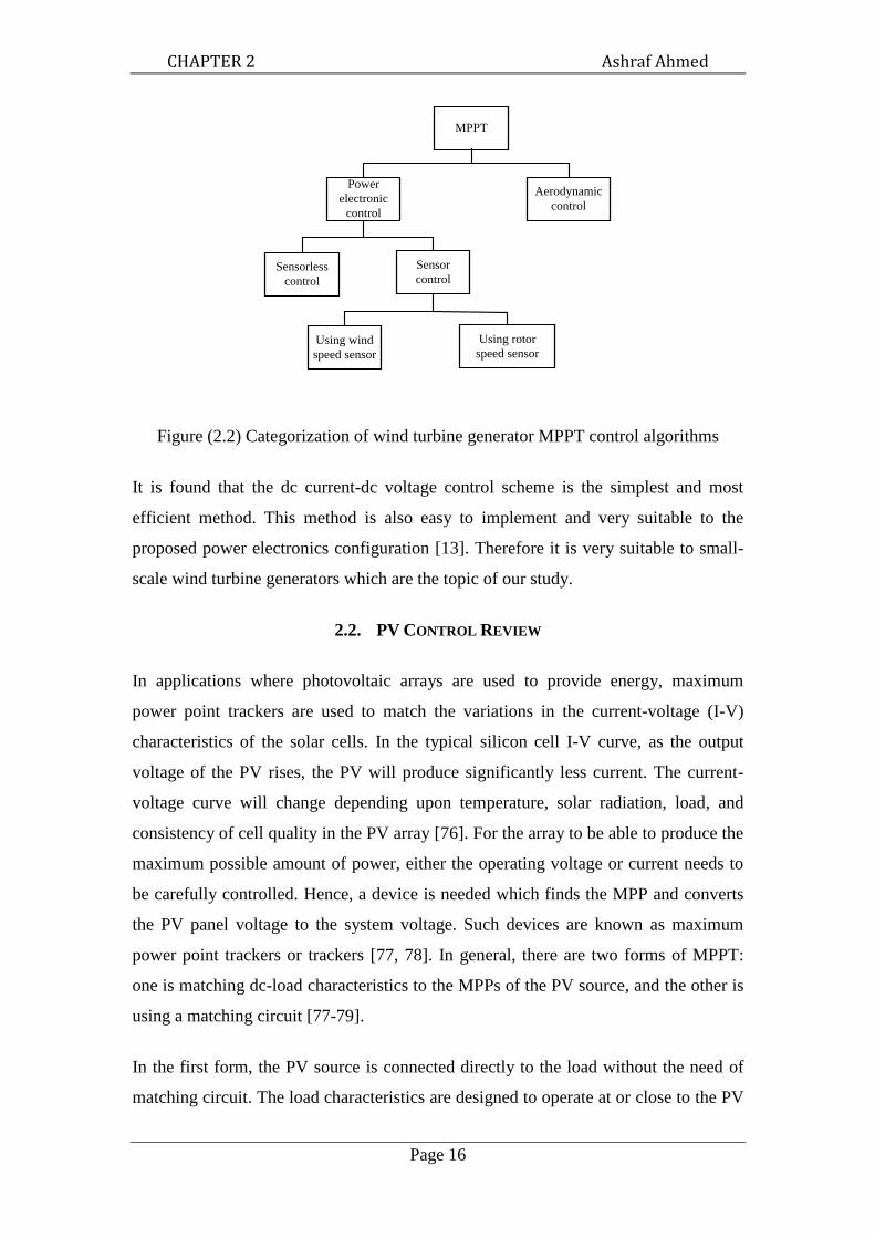
Figure (2.2) Categorization of wind turbine generator MPPT control algorithms
It is found that the dc current-dc voltage control scheme is the simplest and most
efficient method. This method is also easy to implement and very suitable to the
proposed power electronics configuration [13]. Therefore it is very suitable to small-
scale wind turbine generators which are the topic of our study.
2.2. PV CONTROL REVIEW
In applications where photovoltaic arrays are used to provide energy, maximum
power point trackers are used to match the variations in the current-voltage (I-V)
characteristics of the solar cells. In the typical silicon cell I-V curve, as the output
voltage of the PV rises, the PV will produce significantly less current. The current-
voltage curve will change depending upon temperature, solar radiation, load, and
consistency of cell quality in the PV array [76]. For the array to be able to produce the
maximum possible amount of power, either the operating voltage or current needs to
be carefully controlled. Hence, a device is needed which finds the MPP and converts
the PV panel voltage to the system voltage. Such devices are known as maximum
power point trackers or trackers [77, 78]. In general, there are two forms of MPPT:
one is matching dc-load characteristics to the MPPs of the PV source, and the other is
using a matching circuit [77-79].
In the first form, the PV source is connected directly to the load without the need of
matching circuit. The load characteristics are designed to operate at or close to the PV

CHAPTER 2 Ashraf Ahmed
Page 17
generator’s MPPs. This method is mainly used with dc motor loads, where the dc
motor field winding control is designed in such a way that the dc motor characteristics
match the PV source’s MPPs as much as possible [79-82]. One of the drawbacks of
this method is the nonlinearity of the PV system; it is very difficult to make a perfect
matching without considering the system’s temperature, which has a very significant
effect on the PV characteristics. Another drawback is that the tracking efficiency is
reduced when compared with using matching circuits. Also, the method is only
applicable to special loads such as dc motors and batteries.
Many algorithms use a matching circuit for MPPT. These algorithms can be classified
as either direct or indirect methods, depending on the control method employed [83].
Direct methods include algorithms that use measuring currents, voltages, power,
temperature or solar radiation of the solar array. Indirect methods are those which use
an outside signal to estimate the MPP. Such outside signals may be given by
measuring the short circuit current or the open circuit voltage of a reference solar cell
(monitoring cell). A set of physical parameters has to be given, and the maximum
power set point is derived from the monitoring signals. In the following sections, the
direct and indirect methods will be proposed.
2.2.1. DIRECT MPPT METHODS
The direct methods mentioned above are simpler and have a lower cost than the
indirect methods. This is because we will not need to use separate devices as the
monitoring cell. The various direct algorithms will be divided according to the control
variables chosen to achieve the maximum power point tracking control.
A. DATABASE METHOD
In the lookup table method, MPPT is performed by registering the MPPs in an
extensive database of MPP voltages at all light radiation levels. This control algorithm
has several disadvantages but mainly it is only valid with regard to particular PV
panels and the database must be changed as the PV panel degrades. A large memory
lookup table size is needed for a wide range of solar radiation and temperature levels
[84].

CHAPTER 2 Ashraf Ahmed
Page 18
B. OPEN CIRCUIT VOLTAGE CONTROL
The solar array terminal voltage is used as the control variable for the system. The
reference control voltage signal is set with respect to the array open circuit voltage to
determine the maximum power points. The basic function is used to assign the
reference control voltage shown in Equation (2.5) [85]. This method assumes that the
proportionality of voltage-factor (Kv) is fixed for a given PV generator regardless of
temperature, solar radiation, and panel configuration but depends on cell material and
make [86, 87]. This property is used to achieve temperature and solar radiation-
independent MPPT for PV generators with a simple technique. The open circuit
voltage is continuously measured by a microcontroller and is used to estimate the
operating maximum power point of the system. Moreover, this method can be
implemented using an analogue circuit [85].
ocvmppVKV (2.5)
where KV is the voltage proportional constant, Vmpp the MPP voltage and Voc the
open circuit voltage. Obviously, the drawbacks of the voltage control method are
1. The wasted available energy when the load is disconnected from the PV array
to measure the open circuit voltage.
2. It is proposed that the proportional constant of the open circuit voltage (Kv) is
constant with solar radiation and temperature. However, in the reality, the Kv
values vary in the range from 73 to 80% according to solar radiation and
temperature.
3. The degradation in PV array characteristics also affects (Kv) value.
C. SHORT-CIRCUIT CURRENT CONTROL
The short-circuit current is used as the reference parameter in this method. The
reference current is adjusted according to the short-circuit current. This method is
based on the fact that the MPP current is a constant percentage of the short-circuit
current. To implement this algorithm, a switch is placed across the input terminals of
the converter and switched on momentarily. The short-circuit current is measured and
the MPP current calculated from the Equation (2.6):

CHAPTER 2 Ashraf Ahmed
Page 19
scimppIKI (2.6)
where, Ki is the current proportional constant, the PV array output current is then
adjusted by the MPPT until the calculated MPP current is reached [88]. In a more
complicated method, a PV scanning is performed every few minutes in order to
calculate Ki . This scan is performed to overcome the online change of Ki with solar
radiation and temperature, and the PV array degradation effect. After Ki is obtained,
the system remains with the approximation until the next calculation of Ki is carried
out [89].
The drawbacks of the current control method are
1. The available energy is wasted when short-circuiting the PV source.
2. The added complexity in the power electronics to short-circuit the PV source.
3. With the complexity of this method, the method is not acceptable for large
power applications.
D. POWER CONTROL
The system power is used as the control variable, where the power is measured and
adjusted according to the change in the atmospheric conditions. Most of the Power
control algorithms use the hill-climbing method; this method is to climb the power
curve to reach the MPPs. In the following sections several MPPT search algorithms
will be discussed, which make use of different characteristics of solar panels and the
location of the MPPs.
Perturb and observe method (P&O) is the most commonly used MPPT algorithm, due
to its ease of implementation in its basic form [90-94]. Knowledge of the PV
generator characteristics is not required. This method has many modifications: one of
them is to directly use the dc/dc converter duty cycle (D) as a control parameter and
force the derivative dP/dD to be zero, where (P) is the PV array output power [95].
Another modification is to perturb the current instead of the voltage [96]. However,
this method also has some drawbacks such as the continuous oscillations around the
MPP. Also, as the amount of sunlight decreases, the P–V curve flattens out which

CHAPTER 2 Ashraf Ahmed
Page 20
makes it difficult for the MPPT to track the location of the MPP, and it fails under
rapidly changing atmospheric conditions.
The incremental conductance (I.C.) is another searching method which tracks the
MPP accurately by comparing the I.C. and instantaneous conductance of a PV array
[12, 97-100]. This method is based on the principle that at the MPPs:
0dV
dP (2.7)
Because P=VI, the following equation can be derived:
I
V
dI
dV (2.8)
This is the basic rule for the I.C. method where P, V, I are the PV array output power,
voltage and current, respectively. The direction, in which a perturbation must occur to
move the operating point toward the MPPs, is determined as follows:
. (2.9)
There are many variations of this method. One of them is to reduce calculations and
make the algorithm more applicable to the microprocessor [100]. Another
modification is to propose another algorithm which depends on the relationship
between the load line and the tangent line angles of the I-V characteristic curve [101].
The incremental conductance method is faster than the P&O method and it operates
successfully even in cases of rapidly changing atmospheric conditions where the P&O
method fails. This is because it actually calculates the direction in which to perturb the
array’s operating point to reach the MPP, and it can determine when it has actually
reached the MPP. Thus, under rapidly changing conditions, it does not track in the
wrong direction, as the P&O method does. Nor does it oscillate around the MPP once
it reaches it.
There are other power control algorithms which use hill-climbing, but these are
different from the P&O and the I.C.. One proposed algorithm is applying a hybrid
MPPT algorithm of the I.C. and P&O methods [99]. Another method is to use neural

CHAPTER 2 Ashraf Ahmed
Page 21
networks to compute the maximum power point [102-104]. Using fuzzy logic
controllers has the advantage of working with imprecise inputs, not needing an
accurate mathematical model, and being capable of handling nonlinearity [105-108].
An algorithm in reference [109] is based on the analysis of the current and voltage
low-frequency oscillations.
2.2.2. INDIRECT METHOD
The indirect MPPT method proposes that the constant voltage or current method is to
be used, but the open-circuit voltage or short-circuit current measurements are made
on a small solar cell called a pilot cell. This cell has the same characteristics as the
cells in the larger solar array and is subject to the same atmospheric condition. The
pilot cell measurements can be used by the MPPT to operate the main solar array at its
MPP, eliminating the loss of PV power during the VOC
or ISC
measurement. Reference
[110] introduced this algorithm. The disadvantages of this method are as follows:
there will be unavoidable errors due to the mismatch between the characteristics of the
pilot cell and the PV array; the shadow effect is unavoidable; each pilot cell-solar
array pair must be calibrated, increasing the effort required to build the system.
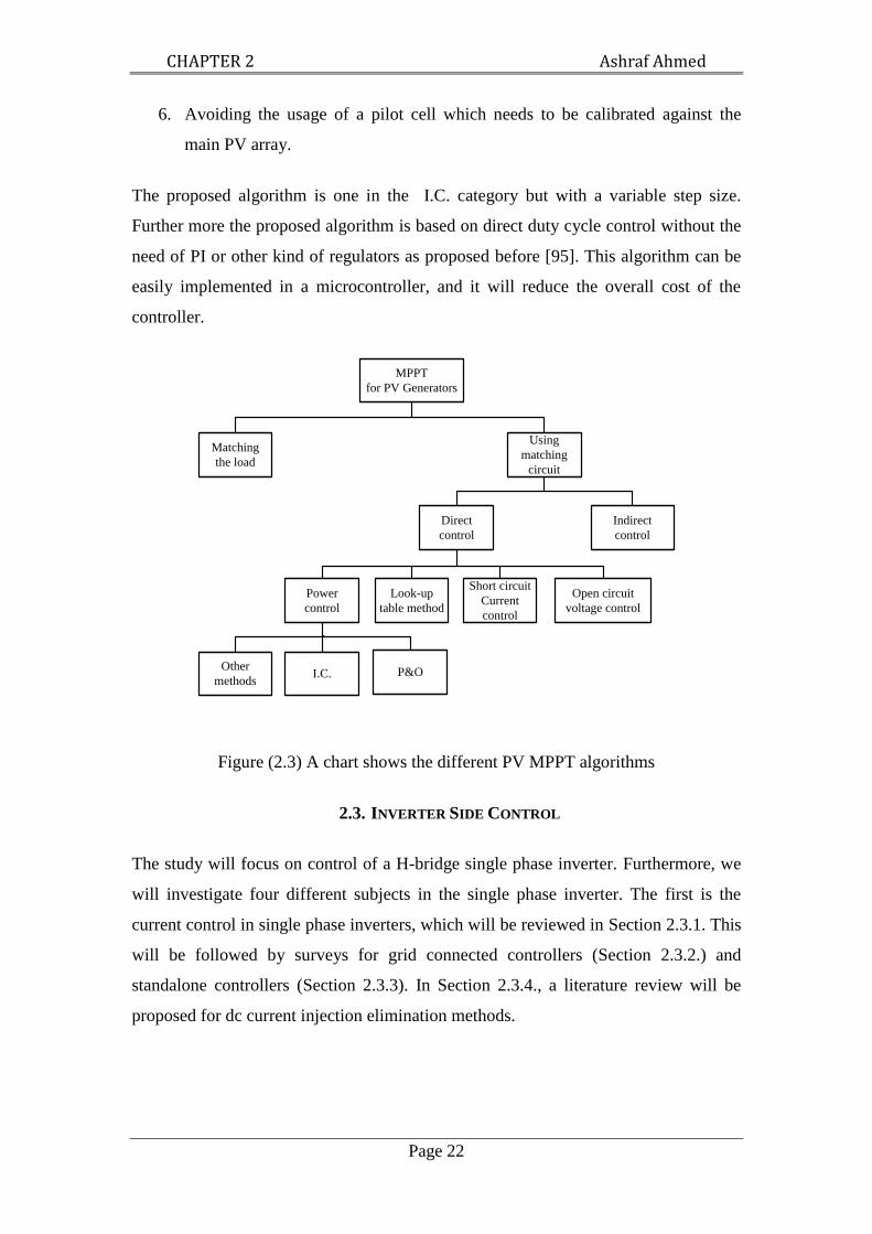
2.2.3 SUMMARY AND GUIDELINES
From the study of the different MPPT algorithms (summarized in Figure (2.3)), a new
MPPT control algorithm will be proposed. It will take into account the drawbacks of
existing algorithms and will have the following advantages:
1. The method is easy to implement in microcontrollers.
2. No extra power electronics are added to the system, which decreases circuit
complexity.
3. There is no energy waste as the load disconnection case from the PV array
with open circuit voltage control or short circuit current control.
4. The controller is generic and can be used with many PV generators without
any changes required to adapt to different PV sizes.
5. Avoiding the usage of costly and bulky solar radiation and temperature
sensors.
CHAPTER 2 Ashraf Ahmed
Page 22
6. Avoiding the usage of a pilot cell which needs to be calibrated against the
main PV array.
The proposed algorithm is one in the I.C. category but with a variable step size.
Further more the proposed algorithm is based on direct duty cycle control without the
need of PI or other kind of regulators as proposed before [95]. This algorithm can be
easily implemented in a microcontroller, and it will reduce the overall cost of the
controller.
MPPT
for PV Generators
Indirect
control
Direct
control
Power
control
Open circuit
voltage control
Matching
the load
Using
matching
circuit
Short circuit
Current
control
Look-up
table method
P&O
Other
methods
I.C.
Figure (2.3) A chart shows the different PV MPPT algorithms
2.3. INVERTER SIDE CONTROL
The study will focus on control of a H-bridge single phase inverter. Furthermore, we
will investigate four different subjects in the single phase inverter. The first is the
current control in single phase inverters, which will be reviewed in Section 2.3.1. This
will be followed by surveys for grid connected controllers (Section 2.3.2.) and
standalone controllers (Section 2.3.3). In Section 2.3.4., a literature review will be
proposed for dc current injection elimination methods.

CHAPTER 2 Ashraf Ahmed
Page 23
2.3.1. CURRENT CONTROL METHODS
Generally, one of the main functions of the current controller is that the output current
should track the applied reference signal with as little error as possible. Furthermore,
the output signal should have acceptable transients without undesirable over- and
undershoots or low dynamic speed response. On the other hand, the total harmonic
distortions should be as low as possible and below the standard threshold values.
These objectives of the current control should be delivered with competitive cost and
size of the converter. With respect to dc/ac converters, the problem is not as direct as
in dc/dc converters. This is because the tracking of a sine wave signal is not as easy or
direct as the tracking of a dc signal. The current control methods of single phase
inverters will be reviewed in the following subsections.
A. LINEAR REGULATOR BASED METHOD
In this method, the output current is controlled by linear regulators associated with a
carrier-based PWM, and it is also called carrier-based method in many studies. There
are many PWM switching strategies proposed to reduce the THD of the output
current. Among these, the sinusoidal PWM methods (unipolar and bipolar) are
commonly used with the H-bridge [111, 112]. Other methods such as centroid based
switching [113], hybrid PWM [114] and random hybrid PWM [115] have also been
proposed to improve the quality of the current wave.
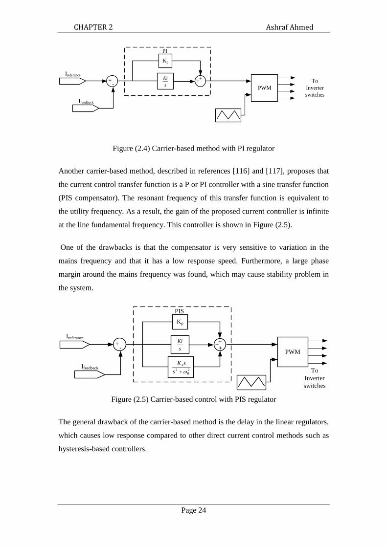
One advantage of the carrier-based control method associated with linear regulators is
the constant switching frequency operation. A simplified diagram describing this
method is shown in Figure (2.4).
Applying PI controller is very common with small-scale inverters [115], but this kind
of controller has relatively poor performance. One reason is the common steady state
error produced by the inability to track the sinusoidal reference. Furthermore, this
controller is unable to reject the noise in the current signal [116].
CHAPTER 2 Ashraf Ahmed
Page 24
Kp
s
KiIreferance
PWM
+-
Ifeedback
To
Inverter
switches
++
PI
Figure (2.4) Carrier-based method with PI regulator
Another carrier-based method, described in references [116] and [117], proposes that
the current control transfer function is a P or PI controller with a sine transfer function
(PIS compensator). The resonant frequency of this transfer function is equivalent to
the utility frequency. As a result, the gain of the proposed current controller is infinite
at the line fundamental frequency. This controller is shown in Figure (2.5).
One of the drawbacks is that the compensator is very sensitive to variation in the
mains frequency and that it has a low response speed. Furthermore, a large phase
margin around the mains frequency was found, which may cause stability problem in
the system.
Kp
20
2 s
sK s
s
KiIreferance
PWM
+-
IfeedbackTo
Inverter
switches
++
+
PIS
Figure (2.5) Carrier-based control with PIS regulator
The general drawback of the carrier-based method is the delay in the linear regulators,
which causes low response compared to other direct current control methods such as
hysteresis-based controllers.
CHAPTER 2 Ashraf Ahmed
Page 25
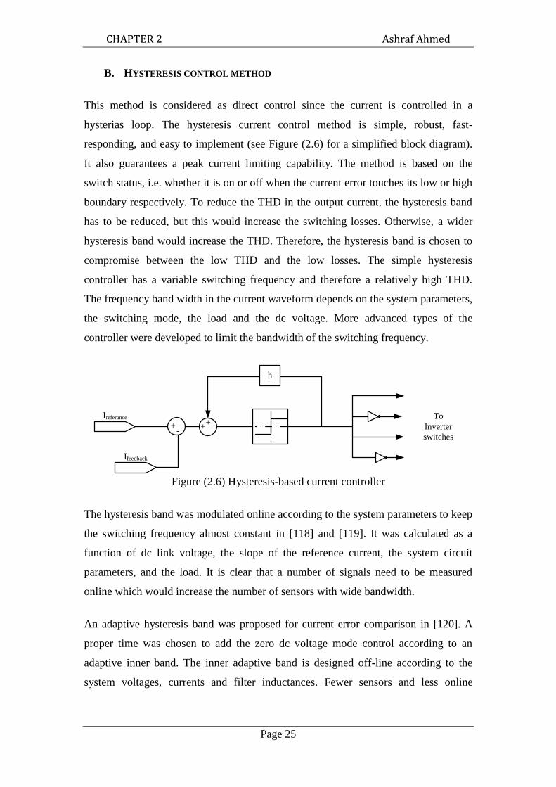
B. HYSTERESIS CONTROL METHOD
This method is considered as direct control since the current is controlled in a
hysterias loop. The hysteresis current control method is simple, robust, fast-
responding, and easy to implement (see Figure (2.6) for a simplified block diagram).
It also guarantees a peak current limiting capability. The method is based on the
switch status, i.e. whether it is on or off when the current error touches its low or high
boundary respectively. To reduce the THD in the output current, the hysteresis band
has to be reduced, but this would increase the switching losses. Otherwise, a wider
hysteresis band would increase the THD. Therefore, the hysteresis band is chosen to
compromise between the low THD and the low losses. The simple hysteresis
controller has a variable switching frequency and therefore a relatively high THD.
The frequency band width in the current waveform depends on the system parameters,
the switching mode, the load and the dc voltage. More advanced types of the
controller were developed to limit the bandwidth of the switching frequency.
Ireferance
+-
Ifeedback
+
+
h
To
Inverter
switches
Figure (2.6) Hysteresis-based current controller
The hysteresis band was modulated online according to the system parameters to keep
the switching frequency almost constant in [118] and [119]. It was calculated as a
function of dc link voltage, the slope of the reference current, the system circuit
parameters, and the load. It is clear that a number of signals need to be measured
online which would increase the number of sensors with wide bandwidth.
An adaptive hysteresis band was proposed for current error comparison in [120]. A
proper time was chosen to add the zero dc voltage mode control according to an
adaptive inner band. The inner adaptive band is designed off-line according to the
system voltages, currents and filter inductances. Fewer sensors and less online

CHAPTER 2 Ashraf Ahmed
Page 26
calculation are needed, compared to the on-line adaptive hysteresis method. However,
the switching frequency change will be higher.
A three-level hysteresis current control strategy for a single phase voltage source
inverter has been proposed in [121]. To achieve this, two hysteresis comparators with
a small offset are used.
The random hysteresis method is one of the most common methods in this field [122].
The method is based on a random number provided to define the upper and the lower
bands of the hysteresis controller. The random signal is distributed to provide an
output current with narrow distributed frequency spectrum contents. Furthermore, the
average frequency can be kept at a low value to reduce the switching losses.
Describing in detail the different algorithms of the random hysteresis method is out of
the scope of this review.
The methods proposed to solve the variable frequency problem of the hysteresis
method could not make the frequency entirely constant. Furthermore, the tolerance
and the variations in the system parameters may disturb the controller. Mainly, these
methods need powerful DSP to perform the calculation.
C. PREDICTIVE CONTROL
The controller predicts the output of the inverter based on the system model.
Subsequently, a suitable sequence of control signals is then applied to grant an
acceptable tracking error. A cost function is minimized to design the predicted control
sequence for the following sampling interval [123-125]. This method was also applied
to parallel connected inverters in this reference [126]. The predictive control method
is entirely based on an effective system model, and a fast high-performance DSP is
essential to perform the calculations every sampling period [127].
2.3.2. GRID-CONNECTED CONTROL
There are many methods to determine the injected active and reactive power to the
grid, depending on the converter topologies, the PWM methods, and the control
techniques. These methods might also be used with active power filters which
compensate for reactive power and distorted currents.

CHAPTER 2 Ashraf Ahmed
Page 27
In single-source systems, the inverter could directly maximize the power from the
source and provide power factor control [94,128 and 129]. The inverter works in this
case as a current controller and the dc input voltage would be variable to provide
MPPT. This method is not suitable for multi-source inverters such as those proposed
in this study where the dc link is shared.
Another method controls the power output of the inverter by controlling the phase
shift between the inverter output (Vinv) and the grid (Vg) voltages (the power angle).
The reactive power is controlled in this method using the modulation index. This
method uses a lookup table to find the required phase shift according to the active and
reactive power demands [130]. The reactive power is very sensitive to the power
angle and accurate design of the controllers is needed. Furthermore, using lookup
tables is not favourable because it causes the controller to be largely affected by the
system parameters as the line inductances.
The p-q method is originally used with three phase systems and was extended to a
single phase case [131-133]. The method is based on separation of instantaneous
active and reactive power in two coordinates, and then the reference current is
calculated [14]. The method was also used with a single-phase inverter supplied by a
PV generator [135]. This method is normally used with PI regulators, which are slow
in response compared to direct regulators.
2.3.3. STANDALONE MODE CONTROL
In the inverter’s standalone mode of operation, the objective is to maintain the ac
output voltage waveform in specified reference over all loading conditions. An easy
method normally used in early uninterruptible power system (UPS) inverters is based
on forward open loop control. The grid voltage magnitude was controlled using an
r.m.s. feedback loop to control the magnitude. This method has a slow response and
no-disturbance reduction to the ac wave [136].
The hysteresis control mentioned before in Section (2.3.1) was used in UPS
applications which have the disadvantages discussed in the same section [137, 138].
Another proposed method is based on estimating the output filter values [139]. The
tolerance, which reaches 20% in practical inductors and capacitors, will affect the

CHAPTER 2 Ashraf Ahmed
Page 28
controller operation for this method. Analogue methods were proposed based on
capacitor current feedback control [140] or inductor current feedback control [141] as
normally the LC-filter is used in UPS applications.
2.3.4. DC -ELIMINATION METHOD REVIEW
The inclusion of a low frequency (50 or 60 Hz) isolation transformer at the output of
the inverter eliminates the injection of dc on the grid side. Drawbacks of using this
type of transformer are the cost, weight, and size added to the inverter system, as well
as the reduced overall efficiency. A low frequency transformer is more bulky than a
high frequency isolation transformer which however cannot prevent dc injection into
the grid [22, 142].
For a transformerless topology, the research to overcome the dc injection problem
could be basically classified into three categories as follow:
B. USING ALTERNATIVE INVERTER TOPOLOGIES
A half bridge inverter has been proposed to remove the dc injection to the grid, but
there are many problems, such as using double dc link voltage, increased losses, and
the large size of the dc link capacitors. This also increases the overall cost and size of
the inverter. Using such a kind of inverter will also increase the ripple and reduce the
total harmonic distortion [14, 18].
Using neutral point diode clamped multilevel is proposed in reference [143]; this has
better efficiency compared to the basic half bridge inverter. However, it still needs
twice of the dc voltage value of the H-bridge, and larger capacitors.
C. MODIFYING THE H-BRIDGE TOPOLOGY
The basic idea is to modify the H-bridge inverter to eliminate the dc component of the
current. One of the topologies is to add switches on the dc side to clamp the voltage
during the zero voltage periods [103]. This idea could also be applied by clamping on
the ac side [20]. Both methods could not guarantee elimination of the dc component
as the unbalance due to forward IGBTs voltages and PWM control would not be
removed.

CHAPTER 2 Ashraf Ahmed
Page 29
D. DC ELIMINATION BY CONTROL
A solution to the dc injection problem is to use a feedback control loop to eliminate
the dc offset in the inverter output voltage, and such an approach is adopted in this
study. Although this was also adopted in previous studies [22, 144-146], a challenge
remaining to be addressed further is the accurate measurement of the usually very
small dc component mixed with a large fundamental ac current component.
Reference [22] proposes a method of auto-calibrating the current sensing device to
remove its error. The dc component on the ac output side of the inverter is deduced
from the reading of the calibrated current sensor on the dc side, assuming the
knowledge of the inverter switching pattern. This method can reduce the dc injection
but will not eliminate it because it only intends to compensate the dc injection due to
inaccuracy in the PWM process, while the dc component caused by unequal on-state
voltage of the semiconductor devices in the inverter cannot be compensated.
Furthermore, the method is subject to the influence of noises and achieves its
objective at the cost of increased inductance between the dc link capacitor bank and
the inverter bridge which should ideally be kept as low as possible to constrain
switching transient and avoid EMC problems.
2.4. SUPERVISORY CONTROL METHODS REVIEW
Hybrid renewable energy systems can be classified into two main types: grid-
connected and standalone. The renewable energy sources can be PV or wind
generators (or both), according to the availability of solar radiation or wind velocity
(or both) at the system site. Batteries are often used as a backup source to supply the
system when the renewable energy source is unavailable. Other backup sources can be
used with or without batteries such as fuel cells (e.g. electrolysers, supercapacitors
and flywheel energy storage). Diesel generators could be used as secondary sources of
renewable energy. The standalone system might provide dc power, ac power, or both
dc and ac power [147-149].
The grid-connected systems can work on standalone mode when the utility grid is
unavailable. In grid-connected systems, the utility grid is a secondary source. For the
most part, fuel cells and diesel generators are not used with such grid-connected

CHAPTER 2 Ashraf Ahmed
Page 30
systems. The supervisory controllers manage the power according to the type and
different components of the system. In this section, a survey of the supervisory
controllers adapted to the different renewable energy systems will be discussed. The
supervisory controllers could be divided generally to two kinds; conventional-based
and artificial intelligence-based methods.
2.4.1. CONVENTIONALLY-BASED METHODS
A small-scale hybrid PV-Wind generation system with batteries works only in
standalone mode as proposed in [63]. The power conditioning unit is limited to
maximize the output power from both the wind and the PV generators to the batteries.
The charging and discharging methods of batteries, over power ratings and load
management, are not taken into account in this system.
A design of a supervisory controller based on a sliding mode control is presented in
reference [150]. The system is a standalone hybrid PV-Wind generation system. For
the design of such a supervisory controller, the wind generator plays the role of the
main generator while the solar generator is a secondary power source. The system has
three modes of operation: in the first mode, the wind generator is regulated to supply
the system while the PV generator is OFF. In the second mode, the wind power is
maximized and the PV power is regulated. Both PV and wind are maximized in the
last mode. In the proposed control strategy, the battery state of charge is not taken into
account. Furthermore, the wind power regulation strategy is not explained.
A wind generation system with storage batteries is controlled to work in both grid and
standalone operation modes discussed in this chapter [147]. The supervisory
controller in this system is designed to provide smooth transitions between the modes.
Furthermore, it controls the inverter, providing fault ride through to limit the output
current during utility grid side faults. This fault ride through strategy is explained in
reference [151].
The supervisory controller of a standalone hybrid Wind-PV-fuel cell (FC) energy
system is proposed in [152-154]. Every source is connected to the ac bus bar via an
inverter to supply the load. The FC–electrolyzer combination is used as a backup and
long-term storage system. The battery bank is used in the system as a short-time
backup to supply the transient power. At any given time, the supervisory controller

CHAPTER 2 Ashraf Ahmed
Page 31
controls any excess wind-PV-generated power to be supplied to the electrolyser. The
hydrogen, which is delivered to the hydrogen storage tanks by a gas compressor, is
consequently generated. If the generated power is less than the load demand, the FC
stack begins to produce energy for the load using hydrogen from the storage tanks. A
steady state model was used in the papers with no dynamical results.
This study demonstrates that the low voltage distribution network is supervised to
optimize energy flow and control power quality [155]. This kind of system is supplied
by renewable energy sources, diesel generators, and energy storage backups. The
system is controlled, according to international power quality standards. The
algorithm is universal and adapts its control variables. This controller is concerned
with the utility grid not with controlling the local generators.
A power mangement program is proposed in refrence [156] for a grid-connected
wind-generated system with energy storage. The energy storage is controlled to
smooth the power output of the energy generation system to the grid. The average
wind velocity is forecast for the next hour and then the energy storage output is
mananged according to the forecast value.
A new scheme of a standalone hybrid PV-Wind system with batteries is proposed in
[157]. The PV is directly connected in parallel with the batteries to supply the ac load
through a three phase inverter which is connected from the other side to a wind
generator. The power management strategy is simplified in this configuration as the
batteries act as a constant voltage load line which charges both ways by the PV and
the wind generators. A dump load can be switched on with batteries fully charged but
the batteries are later disconnected to prevent overcharging. One of the drawbacks is
that there is no ability in this scheme to provide PV or wind generators control.
Furthermore, the batteries’ charging and discharging is not fully controlled.
2.4.2. ARTIFICIAL INTELLIGENCE-BASED METHODS
A standalone system with hybrid PV-diesel power generators and flywheel backup
energy storage system is proposed in [158]. A pump is used as an auxilary load to
absorb the extra power from the system. A fuzzy logic supervisory controller is
proposed to manange the power from the generators to the load. According to the

CHAPTER 2 Ashraf Ahmed
Page 32
generated PV power and the rotor speed of the flywheel, the fuzzy controller adjusts
the refrences for the diesel generator output power and the pump demand.
A fuzzy logic supervisor is proposed also in reference [159] for a grid-connected wind
generated system. The supervisory controller regulates the power of the wind
generator according to the change in the grid frequency. The pitch angle is controlled
to match the reference power generated by the supervisory controller.
The same system used in the last reference is used in this reference [160] with the
exception that there is a flywheel controlled by a fuzzy supervisor to smooth the
output power of the wind generator. A storage capacitor could be used also in the
same manner [161].
In a microgrid system [162], the PV generators could be used to remove frequency
deviations using fuzzy supervisory controller. This controller increases or decreases
the PV output power to match a high frequency or a low frequency respectively.
In reference [163], the fuzzy supervisor controls the pitch angle of a fixed speed wind
generator and the reactive power output of the static VAR compensator to smooth the
wind generator output power and regulate the grid voltage respectively.
A neural networks-based supervisory controller manages the power in a PV
standalone system with batteries. Two neural networks are used: one neural network
for direct control and the second to adapt the first one to optimize the system’s
operation [164].
2.4.3. SUMMARY AND GUIDELINES
The proposed control methods diverge according to the system components, the
system operational modes, and the adopted algorithms. The following points could be
concluded:
1. Using artificial intelligence is not advantageous for such small-scale systems,
as the conventional algorithms are easier to be programmed. Artificial
intelligence might be taken into account if the control process is complicated
or needs online optimization.

CHAPTER 2 Ashraf Ahmed
Page 33
2. Many research papers model only the steady state operation of the system and
do not take transient dynamics into account. This does not give the right
indication about the system’s capability to work in the different modes of
operation. Nevertheless, it will demonstrate the stable transitions between
those modes.
3. Load management is a very important issue in this field of study, as the system
works in standalone mode.
4. Storage means are a vital component in the PV-Wind renewable energy
system. That is due to the disability of such systems to provide 100%
availability, and to improve the quality of the output power.

CHAPTER (3)
CONTROL ON WIND POWER SIDE
3.1. INTRODUCTION
This chapter focuses on the wind turbine generator side of the system. The advantages
of using a VAWT which directly drives a PMSG have already been discussed in
Chapter (1). In this chapter, the control of this configuration will be proposed. The
control of the wind turbine generator aims to deals with two different wind velocity
scenarios:
MPPT control in low and moderate wind velocities when the maximum power
produced and rotor speed is less than the rated value.
High wind velocity control when the output power and rotor speed of the
generator could exceed rated values.
The study in this chapter intends to develop a controller which maximizes the power
of the wind generator at low and moderate wind velocities. As the wind velocity goes
beyond the rated value, the controller limits the output power and rotor speed. The
high wind velocity control is found to be a general problem in VAWTs. It is not easy
to be mechanically stalled because adding mechanical control to the turbine will
significantly complicate the turbine and reduce its reliability. Furthermore, it will
increase cost and size of the turbine. A literature review was presented in Chapter 2,
discussing the different control methods for MPPT and high wind speed control.
The configuration of the proposed wind generation side is shown in Figure (3.1). It
consists of a VAWT driving a PMSG. The main control action for the wind generator
is provided by a boost dc-dc converter, which supplies the power to the inverter.
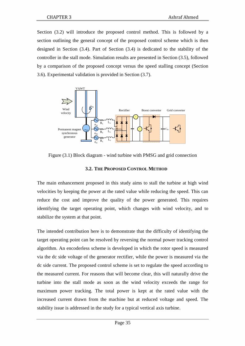
CHAPTER 3 Ashraf Ahmed
Page 35
Section (3.2) will introduce the proposed control method. This is followed by a
section outlining the general concept of the proposed control scheme which is then
designed in Section (3.4). Part of Section (3.4) is dedicated to the stability of the
controller in the stall mode. Simulation results are presented in Section (3.5), followed
by a comparison of the proposed concept versus the speed stalling concept (Section
3.6). Experimental validation is provided in Section (3.7).
Cdc
A
V
Boost converterRectifier
VAWT
Permanent magnet
synchronous
generator
ωm
Wind
velocity
LsRs
LsRs
LsRs
esb
esa
esc
Grid converter
Figure (3.1) Block diagram - wind turbine with PMSG and grid connection
3.2. THE PROPOSED CONTROL METHOD
The main enhancement proposed in this study aims to stall the turbine at high wind
velocities by keeping the power at the rated value while reducing the speed. This can
reduce the cost and improve the quality of the power generated. This requires
identifying the target operating point, which changes with wind velocity, and to
stabilize the system at that point.
The intended contribution here is to demonstrate that the difficulty of identifying the
target operating point can be resolved by reversing the normal power tracking control
algorithm. An encoderless scheme is developed in which the rotor speed is measured
via the dc side voltage of the generator rectifier, while the power is measured via the
dc side current. The proposed control scheme is set to regulate the speed according to
the measured current. For reasons that will become clear, this will naturally drive the
turbine into the stall mode as soon as the wind velocity exceeds the range for
maximum power tracking. The total power is kept at the rated value with the
increased current drawn from the machine but at reduced voltage and speed. The
stability issue is addressed in the study for a typical vertical axis turbine.

CHAPTER 3 Ashraf Ahmed
Page 36
Operation in the MPPT region can be shown to be inherently stable, while operation
in the stall region needs to be stabilized using additional control terms as will be
shown later. The resultant dynamic system is nonlinear and many methods could be
employed to deal with the control problem, including sliding mode [165, 166],
adaptive [167, 168], and predictive control [169], or their combinations. Such
methods may not be easy to implement using a simple micro-controller and may be
difficult to tune. The method proposed is based on designing a PI controller to
regulate the rectifier dc side voltage via generator speed at low wind velocities where
the control objective is MPPT. At high wind velocities, the controller aims to stall the
turbine at rated power and further compensates for stability because normal control
will be unstable in this region. An advantage of the method is the ease of
implementation. Furthermore, the controller tuning process to produce stable soft
stalling is easier and more straightforward.
3.3. CONSTANT POWER SOFT STALLING CONCEPT
The system configuration is shown in Figure (3.1) where the permanent magnet
synchronous generator is represented as a 3-phase Thévenin equivalent feeding into a
diode bridge rectifier. The dc-dc converter controls the power extracted from the
generator, while the grid inverter maintains the power balance to keep the voltage
across the capacitor Cdc constant.
A fixed pitch turbine with a Cp-λ curve, as shown in Figure (3.2) [170], should
normally operate near the maximum efficiency point (Cpmax) by adjusting the speed to
maintain the tip speed ratio at its optimum value, defined here as λmax. If this control is
continued at excessive wind velocities, the electrical power, speed, and voltage will
exceed the rating of the generator and converter. The control method proposed is to
limit the output power and rotor speed by forcing the turbine into the low speed stall
region. To do this the generator output is temporarily increased by the dc-dc converter
to force the turbine to stall. Note that the power coefficient is a function of the tip
speed ratio, which subsequently depends on the rotor speed.

CHAPTER 3 Ashraf Ahmed
Page 37
0 1 2 3 4 50
0.05
0.1
0.15
0.2
0.25
0.3
0.35
CP
Stalling
region
Cpmax
High rotor
speed region
λ
λmax
Figure (3.2) Typical Cp-λ Curve for VAWT
A wind turbine can either increase or decrease its speed to reduce the power capture
by adopting a lowered Cp value. Figure (3.3) shows the rotor peed versus power and
torque of the wind generator. The proposed control decreases the speed which further
prevents the over voltage problem. As the wind velocity increases from the cut-in
value, the rotor speed initially increases for maximum power tracking. Beyond this
region, say >12 m/s wind velocity, power will be kept constant at the rated value. The
intended operating points are A, B and C for wind velocities 15 m/s, 20 m/s and 25
m/s respectively. If the wind velocity later reduces to the region for maximum power
tracking, the controller should detect that and return to the MPPT mode.
The operating points A, B or C are not explicitly obtainable if the wind velocity is
unknown. With a PMSG, the dc side voltage of the machine rectifier is proportional to
the rotor speed. Given the dc side voltage, power is proportional to the current on the
dc side of the rectifier. Based on this, the proposed control is to first establish a
lookup table where the rectifier dc side current is measured to determine the target dc
side voltage (hence speed) as shown in Figure (3.4).
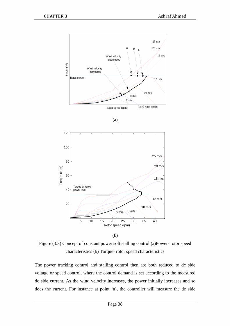
CHAPTER 3 Ashraf Ahmed
Page 38
(a)
(b)
Figure (3.3) Concept of constant power soft stalling control (a)Power- rotor speed
characteristics (b) Torque- rotor speed characteristics
The power tracking control and stalling control then are both reduced to dc side
voltage or speed control, where the control demand is set according to the measured
dc side current. As the wind velocity increases, the power initially increases and so
does the current. For instance at point „a‟, the controller will measure the dc side
Rotor speed (rpm)
Pow
er (
W)
AB
25 m/s
20 m/s
15 m/s
Wind velocity
increases
10 m/s8 m/s
6 m/s
12 m/s
Rated rotor speed
Wind velocity
decreases
Rated power
C
5 10 15 20 25 30 35 400
20
40
60
80
100
120
Rotor speed (rpm)
To
rqu
e (
N.m
) 20 m/s
25 m/s
15 m/s
12 m/s
10 m/s
8 m/s6 m/s
Torque at rated
power level

CHAPTER 3 Ashraf Ahmed
Page 39
current ia and adjust the generator speed so that the dc side voltage reaches va for
optimum power extraction. As the wind velocity continues to increase, the dc side
voltage and current increase to the values corresponding to point „b‟ where the rated
condition is reached. Any further increase of the measured dc side current will require
stalling to enforce a reduced turbine speed and hence dc side voltage. If the controller
continued to work with MPPT, the generator would follow curve (b-c"), which is a
continuation of „o-a-b‟, while with constant speed control the system will follow
curve (b-c‟). Using constant power stalling, the system is forced into curve (b-c)
where the turbine speed can be decreased by temporarily increasing the electrical
power extracted from the generator. The control strategy outlined here for stalling the
turbine is indeed the reverse of what is normally used for MPPT. It is clear that by
reversing the dc side voltage and current as in the conventional power tracking
control, there is no need to explicitly find the operating point of constant power
stalling, which changes with the wind velocity. The stability and dynamic
performance rely on the controller design which is described in the next section.
Figure (3.4) Dc side voltage-current relationship
3.4. SYSTEM MODELING AND CONTROL DESIGN
Referring to Figure (3.3), the generator is controlled in the MPPT mode when the
wind velocity is low, i.e. below 12 m/s. As the wind velocity is increased, the power
extracted from the turbine is maintained at the rated value. The control is based on a
lookup table where the rectifier dc side current is measured to determine the target dc
link voltage as shown in Figure (3.4).
Current (Iw
)
Voltage (
Vw
)
MPPT
region
ia
ic
c
c'b
a
c''
Constant power
stalling
Stalling
region
0
MPPT
va
vc
vb
ib
Constant speed
stalling

CHAPTER 3 Ashraf Ahmed
Page 40
3.4.1. SYSTEM MODELING
The electrical circuit dynamics of the generator have little effect on the overall
mechanical dynamics and can be ignored in the control design. The equivalent circuit
of a permanent magnet generator and the diode rectifier can be simplified as shown in
Figure (3.5) viewed from the dc side of the rectifier. The Thévenin series resistance
Rw has a value of twice the per phase resistance of the generator, neglecting the
commutation overlap in the rectifier as the PM generator used has low inductance.
The source emf (ew), is proportional to the generator speed (ωm).
mwwKe (3.1)
where Kw is a constant depending on the machine design.
Rw
vL
ew
iw
vwωm
Boost
Converter
vs
Tm
Tm
vw
Figure (3.5) A simplified wind generator system
The Thévenin equivalent of the generator and diode bridge rectifier feeds a boost type
dc-dc converter which supplies the dc link of the grid inverter represented as a voltage
source vL. The power drawn by the inverter from the dc link maintains the voltage
constant; with a passive diode rectifier the power level is to be set by the duty cycle
control of the dc-dc converter. The turbine torque is represented by the following
equation.
/)(CARv2
1T
p
2
sm (3.2)
taking into account that (λ) was proposed before in Equation (2.2) (see Chapter (2)).
With a fixed pitch angle, the whole operating region of Cp can be approximated in the
following quadratic form as a function of λ.

CHAPTER 3 Ashraf Ahmed
Page 41
32
2
1paaaC (3.3)
The coefficients of this equation can be obtained using curve fitting techniques.
Values of the coefficients for the turbine used here, with the power characteristic
shown in Figure (3.2), are given in Table (3.1), together with other parameters of the
system.
Neglecting damping and friction, the mechanical dynamics can be reduced to:
em
m TTdt
dJ
(3.4)
ww
m
ww
m
e
eiK
iePT
(3.5)
From Equations (3.1), (3.4) and (3.5),
w
3
s
3
2
s2ws1w
ww
e
vbvbevbi
J
K
dt
de ` (3.6)
where J/RaKb1t1
J/aKKb2wt2
)JR/(aKKb3
2
wt3
AR5.0Kt
On the electrical side, the relationship between the dc side voltage of the rectifier and
the voltage as the input to the grid side inverter can be simplified as
Lwv)d1(v (3.7)
The average dc side current can be calculated as follows.
]v)d1(e[R
1i
Lw
w
w (3.8)
Linearization and combination of Equations (3.6), (3.7) and (3.8) gives the following
equation which represents the total system dynamics.
s3L21w1
w vBvBdBeAdt
de (3.9)

CHAPTER 3 Ashraf Ahmed
Page 42
where 2
0w
3
0s30s1w
2
w1E/VbVb)JR/(KA
)JR/(VKBw0L
2
w1
)JR/()D1(KBw0
2
w2
0w
2
0s30s20w13E/Vb3Vb2EbB
Table (3.1) PMSG and wind turbine parameters
Parameters values
Wind turbine rated wind velocity
System output power, rated
value
Generator rated current
Turbine radius
Generator rated voltage
Generator inductance
Generator resistance
Generator emf constant
a1
a2
a3
VL0
Moment of inertia
12 m/s
1 kW
3.4 A
1 m
240 V
1.7 mH
2.1 Ω
10.48
V/(rad/s)
.037
.011
-.0035
400 V
5 kg.m2
Based on the dynamic model, a controller, as shown in Figure (3.6), can be designed.
The control objective is to force the turbine to a specific speed according to the
measured dc side current by means of power control, as implied by Figure (3.4).
The encoderless speed control is implemented by controlling the average dc side
voltage at the rectifier output. vw =f(iw) is a lookup table relating the dc side current
and the reference dc side voltage. The transfer function of the PI controller in the
speed loop is defined as
s
KsK)s(C
ip
(3.10)

CHAPTER 3 Ashraf Ahmed
Page 43
C(s)d
vL
vs(m/s)
iw
vw
- WG
System
vw=f(iw)
+
Figure (3.6) PI control algorithm
where gains Kp and Ki are determined based on the linearized system model at the
rated wind velocity. The Ziegler-Nichols tuning algorithm, built in the Matlab Control
System Toolbox, was used to determine the values for the test system: Kp=-0.38 and
Ki= -0.11. Empirically this would give a satisfactory step response of the model.
Figure (3.7) shows how the real part of the poles of the closed-loop system changes as
the wind velocity increases. The poles are obtained using the closed-loop transfer
function which can be derived from the above relationships. Below 12 m/s, the real
part is negative. It becomes positive and the system is unstable when the wind
velocity is above 12 m/s. This is true for all values of Kp and Ki due to the operation
in the stall region.
Figure (3.7) Stability analysis of original control algorithm
5 10 15 20 25-3
-2
-1
0
1
2
Wind velocity (m/s)
Real part
of
clo
sed-loop p
ole
vs=12 m/s
vs=13 m/s
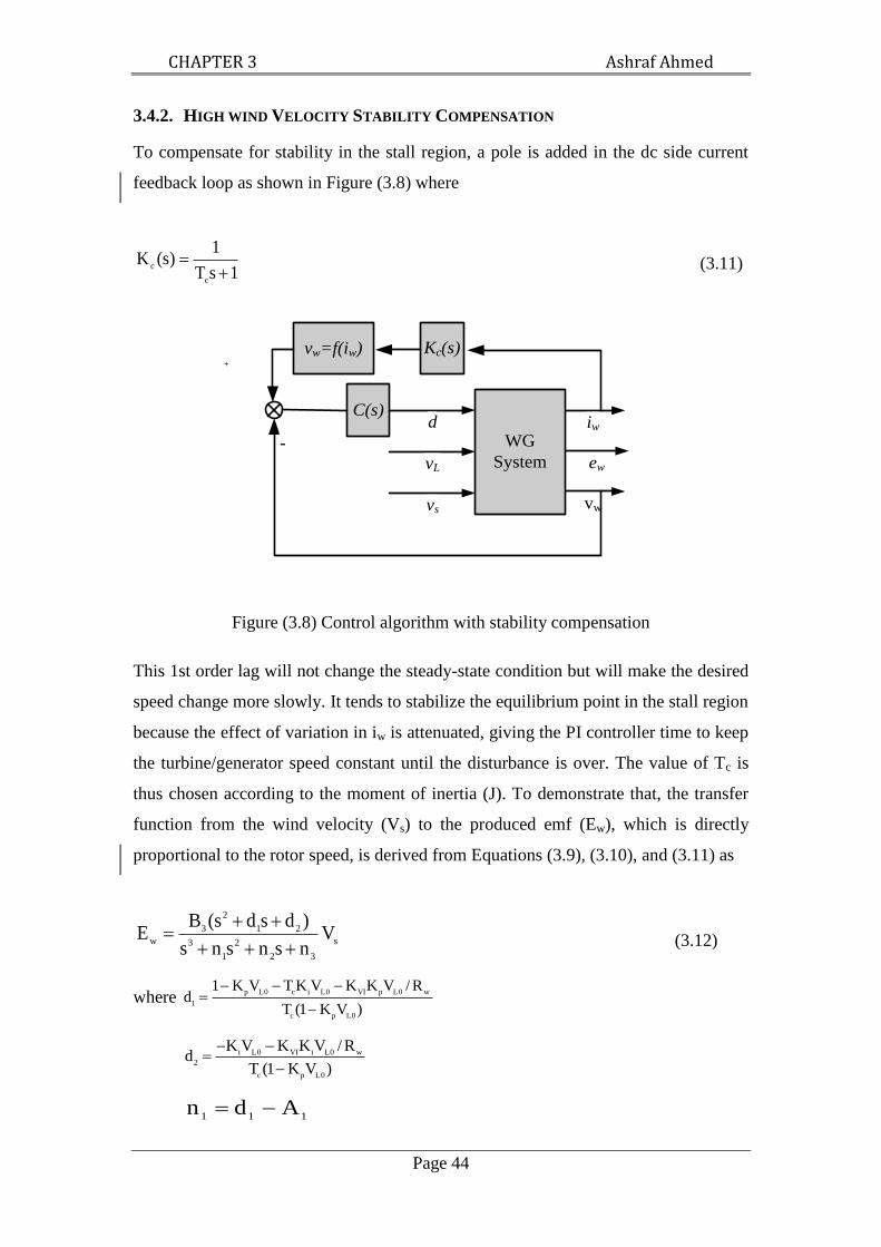
CHAPTER 3 Ashraf Ahmed
Page 44
3.4.2. HIGH WIND VELOCITY STABILITY COMPENSATION
To compensate for stability in the stall region, a pole is added in the dc side current
feedback loop as shown in Figure (3.8) where
1sT
1)s(K
c
c
(3.11)
C(s)d
vL
vs
iw
vw
- WG
System
Kc(s)vw=f(iw)
ew
Figure (3.8) Control algorithm with stability compensation
This 1st order lag will not change the steady-state condition but will make the desired
speed change more slowly. It tends to stabilize the equilibrium point in the stall region
because the effect of variation in iw is attenuated, giving the PI controller time to keep
the turbine/generator speed constant until the disturbance is over. The value of Tc is
thus chosen according to the moment of inertia (J). To demonstrate that, the transfer
function from the wind velocity (Vs) to the produced emf (Ew), which is directly
proportional to the rotor speed, is derived from Equations (3.9), (3.10), and (3.11) as
s
32
2
1
3
21
2
3
wV
nsnsns
)dsds(BE
(3.12)
where )VK1(T
R/VKKVKTVK1d
0Lpc
w0LpVI0Lic0Lp
1
)VK1(T
R/VKKVKd
0Lpc
w0LiVI0Li
2
111Adn
+

CHAPTER 3 Ashraf Ahmed
Page 45
11
p0Lcw
pVI1
22Ad
)KV1(TR
KKBdn
12
p0Lcw
iVI1
3Ad
)KV1(TR
KKBn
20w1VImIm2K
where m1 and m2 are the coefficients of a quadratic curve-fitting function for the
entire V-I characteristics shown in Figure (3.4), which are used in the control design.
It is noted that the designed controller can be further tuned on a computer model using
a more accurate representation (e.g. a lookup table) of the desired V-I relationship.
3w2
2
w1wmImImV (3.13)
Figure (3.9) shows the loci of the dominant roots of the closed-loop system against the
time constant Tc. Without the 1st order lag, the system is unstable as soon as the
increased wind velocity activates the stalling operating mode. As Tc increases, the real
part of the roots moves towards the left-hand side of the complex plane and the
system is stabilized. Targeting a maximum wind velocity of 25 m/s, it is found that for
the test system the minimum value of Tc (in seconds) is about the same as the moment
of inertia J (in kg.m2). This is incidental and depends on the maximum wind velocity
chosen.
For more clarification, the two dominant real parts of the real pole are plotted versus
the wind velocity and Tc. That is shown in Figures (3.10 and 3.11), which are plotted
for inertia of 8 kg.m2. It is clear that the poles are stable as the wind velocity is less
than 12 m/s for all the values of Tc. At high wind velocities, as Tc increases, the poles
are closer to the stable region. According to that, the instability in the system can be
compensated by adding such a pole in the average dc current (iw) feedback loop.

CHAPTER 3 Ashraf Ahmed
Page 46
Figure (3.9) Root locus of closed-loop system
Figure (3.10) First pole with inertia=8
-0.5 0 0.5 1 1.5
-1
-0.5
0
0.5
1
Real axis
Ima
gin
ary
axis
IncreasingT
c
vs=15 m/sv
s=20 m/s
vs=25 m/s

CHAPTER 3 Ashraf Ahmed
Page 47
Figure (3.11) Second pole with inertia=8
The effect of moment of inertia (J) on the stabilizing Tc value is shown in Figure
(3.12). The figure plots the change of the real part of the dominant pole with wind
velocity and Tc for two different values of (J). The plotted wind velocity range is in
the stalling region, which is from 12 m/s to 25 m/s. The figure demonstrates that, as
the inertia increases, the system will be stable at a higher value of Tc. It is found that
choosing Tc slightly greater than the value of the inertia (J) is sufficient to stabilize the
system with an acceptable margin.
The aerodynamic characteristic of a VAWT relies on many factors including the
solidity. Higher solidity means that the Cp-λ curve will have a narrower range of λ,
and the maximum Cp will occur at a lower λ [170].
The turbine in this study has a medium solidity, self-starting torque, and rigid design;
the tip speed ratio values seen in Figure (3.2) are on the low side compared to some
other turbines. The solidity will also affect the moment of inertia which has been
shown to be important in the controller design. It is noted that the thrust force on the
rotor generally reduces as the turbine is sent into the stall region [25]. While it is
expected that the concept of constant power soft stalling can be applied to many
different types of vertical axis wind turbines, a customized design of the controller

CHAPTER 3 Ashraf Ahmed
Page 48
will be necessary to recognize the characteristics of individual turbine series. It is
hoped that this study provides a useful guideline for such an exercise.
12
16
20
24
Figure (3.12) Effect of inertia on the value of Tc to stabilize the system
3.4.3. ADAPTIVE SOFT STALLING CONTROL LOOP
A method has been proposed to compensate for the stability of the system operating in
the stall mode by adding a pole (1st order lag) in the current feedback loop as shown
in Figure (3.8). This is only needed at overrating wind velocities. At low wind
velocities, the system is inherently stable and using it will result in sluggish response
reducing the MPPT efficiency. To delay feedback at high wind velocities and to avoid
MPPT efficiency reduction, an adaptive time constant (Tc) is proposed. The time
constant value needs to be high at high wind velocities and zero at low wind
velocities; therefore, Tc is calculated online as a function of the average dc side
current of the diode rectifier.
1s)i(T
1)s(K
wc
c
(3.14)

CHAPTER 3 Ashraf Ahmed
Page 49
The effect of using such an adaptive feedback is demonstrated by simulation in Figure
(3.13) for the test system where a step change of wind velocity (from 0 m/s to 12 m/s)
is applied at t=15 s. The output power response shows faster tracking capability using
the adaptive delay control loop (Tc=0) as compared to a fixed time constant (Tc=J)
needed to stabilize the system at the highest wind velocity. A block diagram for the
proposed controller is shown in Figure (3.14).
Figure (3.13) Adaptive control loop effect
Measured DC
current (Iw)
Measured DC
voltage (Vw)
Lookup
table
Vw(Iw)Adaptive
current
loop
PI
Controller
with anti-
windup
Control
signal
1/T
-
+
- +
Controller
Figure (3.14) The proposed controller
3.5. SIMULATION RESULTS
The system simulated is grid-connected as shown in Figure (3.1), and has an S1210
H-type Darrieus VAWT driving a PMSG [170]. The PMSG supplies power to the grid
through the power electronics interface stage as described here. The boost converter
10 20 30 40 50 60 700
200
400
600
800
1000
Time (s)
Po
we
r (W
) with adaptive delay
without adaptive delay

CHAPTER 3 Ashraf Ahmed
Page 50
acts as the wind generator controller. The Cp-λ curve of the turbine is the same as
shown previously in Figure (3.2).
A set of simulation results are presented in Figure (3.15) and Figure (3.16), showing
the wind velocity, diode rectifier dc side voltage, dc side current, and the output
power. The target power is also shown for the wind turbine generator in the grey line
according to the same wind profile. In Figure (3.15), the wind velocity changes
between 3 m/s and 12 m/s while in Figure (3.16) it changes between 6 m/s and 24 m/s.
Figure (3.15) shows the results for the system working in the MPPT mode of
operation, as the wind velocities were under the rated value (12 m/s). The figure
shows that the target maximum power curve is tracked accurately by the proposed
controller. The wind velocity increases to slightly less than the rated value at t=100 s
in the time scale. According to this, the power output reaches near to the rated value
(1000 W). The figure also shows that, even with highly turbulent wind velocity data,
the MPPT process is performed without any problem.
For Figure (3.16), focus first on the period between t=120 s and t=160 s. The
controller works in the MPPT mode because the wind velocity is below 12 m/s and
the output power is correspondingly less than the rated value (1000 W). Then consider
the period from t=200 s to t=400 s, when the wind velocity is consistently above 12
m/s. The dc side voltage of the diode rectifier is minimum at t=240 s, and this occurs
when the wind velocity is at the maximum of about 24 m/s. The power during this
period is controlled almost constantly at the rated value, showing that the system is
indeed operating in the soft stall mode. The output power from the generator tracks
the target power in all the regions.
The largest power increase occurs around t=460 s, caused by a fast increase of wind
velocity from 13 m/s to 18.5 m/s in less than 1 s (see also Figure (3.16)). The
turbulence is faster than the wind generator system‟s rotor dynamics. Figure (3.16)
shows the fast increase in wind speed between t=458 and t=459. This caused the
mechanical (Tm) and the electrical (Te) torques to increase as the rotor speed could not
be decreased instantly by the controller. The reason for this is the inertia of the rotor
and the small delay in the electrical system. As a result, the control response is
delayed and the power temporarily exceeds the nominal 1000 W, which should be

CHAPTER 3 Ashraf Ahmed
Page 51
taken into account in semiconductor device rating but has little effect on the cooling
design. As is to be confirmed later by the test results, such power spikes are inevitable
when the wind velocity during a gust quickly increases beyond its rated value.
However the amplitude of the resulting power “spike” is significantly lower than the
power level that would result if the proposed control method were not used. This is
illustrated next.
Figure (3.15) Simulation results with wind velocities lower than the rated values
0 50 100 150 2000
5
10
Win
d v
elo
city
(m/s
)
0 50 100 150 2000
100
200
300
Voltage (
V)
0 50 100 150 2000
1
2
3
Curr
ent
(A)
0 50 100 150 2000
500
1000
Pow
er
(W)
Time (s)
Target power
Output power

CHAPTER 3 Ashraf Ahmed
Page 52
Figure (3.16) Simulation results with wind velocities higher than the rated values
0 50 100 150 200 250 300 350 400 450 5005
10
15
20
25W
ind v
elo
city
(m/s
)
0 50 100 150 200 250 300 350 400 450 500200
250
300
Voltage (
V)
0 50 100 150 200 250 300 350 400 450 5000
2
4
6
Curr
ent
(A)
0 50 100 150 200 250 300 350 400 450 5000
1000
2000
Pow
er
(W)
Time (s)
Output curve
Target curve
vs>12 m/s
vs< 12 m/s

CHAPTER 3 Ashraf Ahmed
Page 53
Figure (3.17) Fluctuations due to rapid wind velocity change
458 459 460 461 462 463 464 465
15
20W
ind v
elo
city
(m
/s)
458 459 460 461 462 463 464 46530
35
Roto
r speed
(ra
d/s
)
458 459 460 461 462 463 464 46530
40
50
60
Torq
ue (
N.m
)
458 459 460 461 462 463 464 4651000
1500
Pow
er
(W)
Time (s)
Tm
Te
High wind velocity
rate of icrease

CHAPTER 3 Ashraf Ahmed
Page 54
3.6. CONSTANT SPEED VERSUS CONSTANT POWER STALLING
To compare constant power stalling with constant speed soft stalling, both strategies
are applied to the same system, with the same wind velocity data. The dc output
power, current, and voltage responses are contrasted in Figure (3.18). The output
power and current voltage in constant power soft stalling are lower than that in
constant speed stalling at wind velocities above rated. The figure also shows that
constant power stalling does not affect MPPT because with wind velocity below 12
m/s the power is the same in both cases, except in the initialization stage of the
simulation.
In the high wind velocity range, the response in constant speed stalling reaches 2000
W, while in constant power stalling it just fluctuates around the rated power and only
temporarily reaches 1200 W. Therefore, the electrical system needs to be over rated
for constant speed stalling to withstand the large power at high wind velocities. This
will increase the size and cost of the system, including the cooling design for the
power semiconductor devices, which have relatively short thermal time constants. The
problem is largely attenuated in constant power stalling.
A dynamic thermal model was built in the Matlab/Simulink with Plecs software for
the PMSG, using parameters of the simulated generator [171]. The PMSG
temperature according to both control methods is shown in Figure (3.19). The figure
clearly shows the advantage of the proposed method with respect to the constant
speed stalling method. Hence, the temperature rise in the proposed method is always
reduced.

CHAPTER 3 Ashraf Ahmed
Page 55
Figure (3.18) Power output: constant power stalling vs constant speed stalling
0 50 100 150 200 250 300 3500
10
20
30W
ind v
elo
city
(m
/s)
0 50 100 150 200 250 300 3500
100
200
300
Voltage (
V)
0 50 100 150 200 250 300 3500
3
6
9
Curr
ent
(A)
0 50 100 150 200 250 300 3500
1000
2000
Pow
er
(W)
Time (s)
Constant power stalling
Constant speed stalling

CHAPTER 3 Ashraf Ahmed
Page 56
Figure (3.19) PMSG Temperature rise with constant speed stalling and constant
power stalling methods
3.7. EXPERIMENTAL VERIFICATION
The active soft stalling concept at excessive wind velocities, as developed in this
study, can prevent complex aerodynamic control and also smooth the power supplied
to the grid. To verify the control method, a laboratory test is carried out and Figure
(3.20) shows a picture of the test rig setup. A simplified block diagram, Figure (3.21),
outlines the hardware arrangement.
The vertical axis wind turbine itself is emulated by an induction motor (IM) driving a
PMSG through a step-down gear box. The IM is driven by an inverter working in the
torque control mode where the torque demand is set according to the measured
rotational speed and the given wind velocity. The same turbine characteristic of the
1000 W system as shown previously in Figure (3.1) are implemented using a desktop
computer hosting a dSPACE real time control system which can be programmed in
the Matlab/Simulink environment [172]. The system parameters and the control gains
are the same as those used in simulation. The generated power is returned to the grid
through a commercially available WindyBoy inverter („Load‟ in Figure (3.21) set to
regulate its dc link voltage.
A simple block diagram reveals the wind turbine model shown in Figure (3.22), as the
inputs of the model are the rotor speed measured signal and the wind velocity data.
0 100 200 300 400 500 60025
30
35
40
45
50
55
60
65
Time (s)
Te
mp
era
ture
(C
o)
Electrical Constant Speed stalling
Electrical ConstantPower stalling
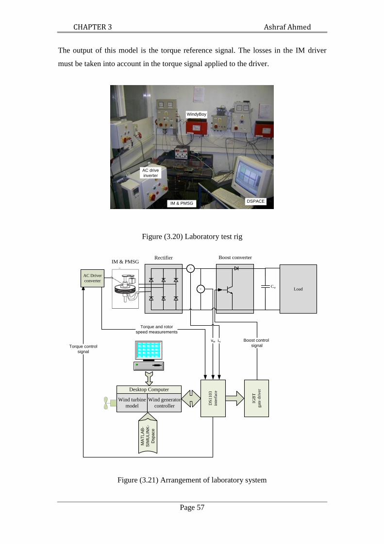
CHAPTER 3 Ashraf Ahmed
Page 57
The output of this model is the torque reference signal. The losses in the IM driver
must be taken into account in the torque signal applied to the driver.
DSPACE
WindyBoy
AC drive
inverter
IM & PMSG
Figure (3.20) Laboratory test rig
Desktop Computer
Wind turbine
model
Wind generator
controller
Cw
A
V Load
Boost converterRectifier
DS
1103
inte
rfac
e
IGB
T
gat
e dri
ver
MA
TL
AB
-
SIM
UL
INK
-
Dsp
ace
Torque and rotor
speed measurements
vw iw
Torque control
signal
AC Driver
converter
Boost control
signal
IM & PMSG
Figure (3.21) Arrangement of laboratory system
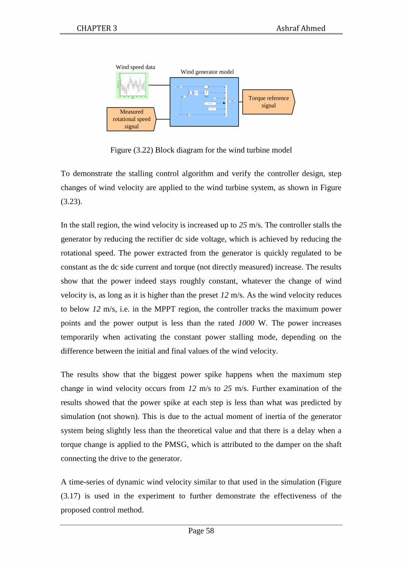
CHAPTER 3 Ashraf Ahmed
Page 58
Measured
rotational speed
signal
Torque reference
signal
Wind speed data
1
Tm
-K-
u^3
Cp as function
in lambada
pi*R_turbine^2
air_dens
.5
2
wm
1
wsws ws 3
0 100 200 300 400 500 6006
8
10
12
14
16
18
20
22
24
26
win
d s
pe
ed
(m
/s)
time(s)
Wind generator model
Figure (3.22) Block diagram for the wind turbine model
To demonstrate the stalling control algorithm and verify the controller design, step
changes of wind velocity are applied to the wind turbine system, as shown in Figure
(3.23).
In the stall region, the wind velocity is increased up to 25 m/s. The controller stalls the
generator by reducing the rectifier dc side voltage, which is achieved by reducing the
rotational speed. The power extracted from the generator is quickly regulated to be
constant as the dc side current and torque (not directly measured) increase. The results
show that the power indeed stays roughly constant, whatever the change of wind
velocity is, as long as it is higher than the preset 12 m/s. As the wind velocity reduces
to below 12 m/s, i.e. in the MPPT region, the controller tracks the maximum power
points and the power output is less than the rated 1000 W. The power increases
temporarily when activating the constant power stalling mode, depending on the
difference between the initial and final values of the wind velocity.
The results show that the biggest power spike happens when the maximum step
change in wind velocity occurs from 12 m/s to 25 m/s. Further examination of the
results showed that the power spike at each step is less than what was predicted by
simulation (not shown). This is due to the actual moment of inertia of the generator
system being slightly less than the theoretical value and that there is a delay when a
torque change is applied to the PMSG, which is attributed to the damper on the shaft
connecting the drive to the generator.
A time-series of dynamic wind velocity similar to that used in the simulation (Figure
(3.17) is used in the experiment to further demonstrate the effectiveness of the
proposed control method.

CHAPTER 3 Ashraf Ahmed
Page 59
The experimental results are shown in Figure (3.24). At t=30 s, the wind velocity
increases above 12 m/s. Therefore, the controller reduces the rectifier dc side voltage
by driving the system into the stall region. The dc side current increases and the
power is almost constant around 1000 W even with wind velocity being over 20 m/s.
As the wind velocity returns to below 12 m/s at around t=280 s, the system resumes
the MPPT control mode and the generated power is less than 1000 W.
The power response contains spikes with the largest occurring at about t=320 s; this is
because at that time the wind velocity increases at a high rate. Another observation is
that the power spike at t=320 s with wind velocity of 17 m/s is higher than that at
t=410 s with wind velocity of 23 m/s, implying that the power spike depends on the
rate of change of the wind velocity.

CHAPTER 3 Ashraf Ahmed
Page 60
Figure (3.23) Experimental results with step changes in wind velocity
0 100 200 300 400 500 600 700 800
10
15
20
25
Win
d v
elo
city (
m/s
)
0 200 400 600 800200
250
300
Voltage (
V)
0 100 200 300 400 500 600 700 8002
4
6
Curr
ent
(A)
0 100 200 300 400 500 600 700 800600
800
1000
1200
1400
Time(s)
Pow
er
(W)
MPPT
regionStalling
region
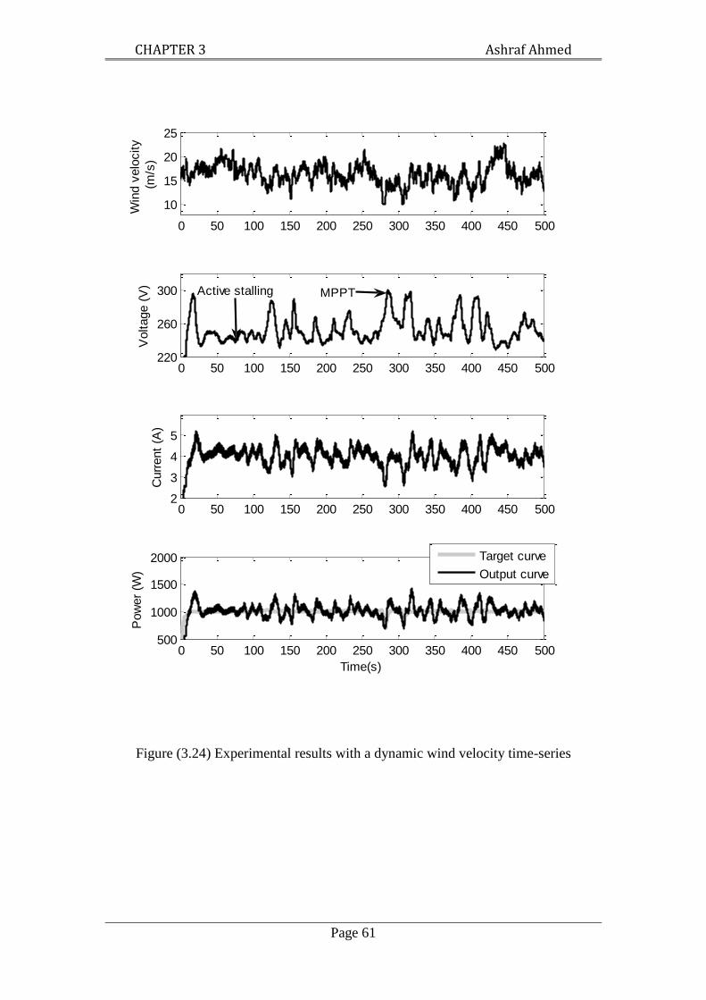
CHAPTER 3 Ashraf Ahmed
Page 61
Figure (3.24) Experimental results with a dynamic wind velocity time-series
0 50 100 150 200 250 300 350 400 450 500
10
15
20
25W
ind v
elo
city
(m/s
)
0 50 100 150 200 250 300 350 400 450 500220
260
300
Voltage (
V)
0 50 100 150 200 250 300 350 400 450 5002
3
4
5
Curr
ent
(A)
0 50 100 150 200 250 300 350 400 450 500500
1000
1500
2000
Time(s)
Pow
er
(W)
Target curve
Output curve
Active stalling MPPT

CHAPTER (4)
CONTROL ON PV POWER SIDE
4.1. INTRODUCTION
This chapter discusses the control of the PV generator in a small scale hybrid PV-
Wind generation system, which could be applied generally in multi-source renewable
energy systems. The PV generator is controlled to provide maximum power point
tracking (MPPT) control or reduced power control according to a signal from the
supervisory controller. Many methods have been applied to achieve maximum power
point tracking (MPPT) control in photovoltaic (PV) power generation systems, as
discussed before in Chapter (2). These methods, with a wide variety of algorithms for
implementation, include open circuit voltage control, short circuit current control, hill
climbing, pilot cells and artificial intelligence techniques. Hill climbing, which is
widely used, can be divided mainly into perturb and observe (P&O) and incremental
conductance (I.C.) algorithms. The hill climbing approach has the advantages of low
cost, generality and ease of implementation. Hill climbing can directly set the duty
cycle of the dc/dc converter to control the PV generating system [195, 173]. Direct
duty cycle control can be easily implemented without the need for a PI controller, and
it will also increase the generality of the method.
As this study is a part of a multi-source small-scale renewable energy system
connected to the grid, the research will provide reduced power mode. The reasons of
the need for such mode of operation will be discussed in details in Subsection (4.4.2).
The objectives of the study in this chapter are as follows:
1. Developing a version of the direct hill climbing algorithm which is more
suitable to hybrid PV-Wind systems.

CHAPTER 4 Ashraf Ahmed
Page 63
2. Dealing with the over rating power problem by developing a reduced power
control mode.
3. Analyzing the dynamic behavior of the system.
4. The direct MPPT control parameters, which are duty perturbation value (δdp)
and the required time between consecutive perturbations (δTp), will be
designed. Furthermore, general guidelines for the design will be provided.
5. Providing simulation and experimental results for verification.
The PV generating system proposed in this study is connected to a grid inverter
through a boost stage, which is commonly used in a multi-source renewable energy
system. A block diagram of the system is shown in Figure (4.1). First, the PV
generator model will be developed in Section (4.2). Then, A design of the
perturbation parameters is developed based on transient analysis of the circuit shown
in Figure (4.1). The proposed control method, based on a variable step incremental
conductance with reduced power mode, is presented at the end of the chapter.
Cdc
A
V
Boost converter
IGB
T
gat
e dri
ver
Boost control
signal
Cin
D
L
MPPT controller
Ipv
Vpv
Vpv
Ipv
PV
Generator
Grid inverter
Figure (4.1) A block diagram of the proposed system

CHAPTER 4 Ashraf Ahmed
Page 64
4.2. PV GENERATOR MODEL
The PV generator is an array of PV modules connected in series and parallel; a PV
module is an array of solar cells. A detailed PV solar cell electrical model is used in
this study based on the Shockley diode equation. The same model for the solar cell is
used for the module taking into account the number of cells in the module [174-177].
The PV generator output power is a nonlinear function of the solar radiation, cell
temperature, and load condition. Many models which are derived from physics, using
curve fitting or artificial intelligence, have been proposed [77]. In this work, a
previously proposed model [177] is adopted because the emphasis here is control.
This model is based on the single diode assumption, while the parameters can be
extracted from the PV module datasheet. In the single diode assumption, the solar
cell, PV module or PV array can be simplified to an equivalent circuit of a diode and a
current source connected in parallel. The current source represents the generated
photocurrent when the sunlight hits the solar panel, and the diode represents the P-N
transition area of the solar cell. The series and parallel resistances represent the losses
due to the body of the semiconductor and the contacts. The equivalent circuit of the
solar cell is shown in Figure (4.2).
Rs
Rsh
Ipv
Idiode IshIlight
Figure (4.2) the solar cell model
The current relationship of the simplified solar cell can be derived from Kirchhoff’s
current law:
shdiodelightpv IIII (4.1)

CHAPTER 4 Ashraf Ahmed
Page 65
where Ipv is the output current, Ilight the light generated current, Idiode the diode current
and Ish the shunt resistance current. Subsequently, the output current (Ipv) can be
calculated as in Equation (4.2). In this equation, the last term can be neglected by
assuming that the shunt resistance (Rsh) is very large. Equation (4.2) is the solar cell
model which can be used as the model of a module by considering that the whole
module is working as a large- area solar cell.
sh
spvA
RIV
0lightpvR
RIV1)(eIII
spvpv
(4.2)
The equations to calculate the parameters Rs, Rsh, A, I0, are provided in (137). Ilight can
be calculated from Equation (4.3).
(4.3)
where
q
mKTA (4.4)
where m depends on the recombination of the carriers in the junction. For a non-ideal
junction, in which some carriers do recombine in the junction, (m) has a value
between 1, 2.
The light-generated current (Ilight) is nearly equal to the short circuit current (Isc), and
is directly proportional to the solar radiation and cell temperature. From the reference
conditions (Sref, Tc_ref), the light-generated current can be calculated from the
following equation as a function of solar radiation (S) and cell temperature (Tc):
))TT(I(S
SII
ref_ccIscref_sc
ref
sclight (4.5)
At a fixed radiation level, increasing temperature leads to decreased open circuit
voltage and slightly increased short circuit current. The increase in the short circuit
current is due to the increase of the minority carriers’ diffusion lengths and the small
reduction of the band gap. In order for this model to reproduce these effects, it is

CHAPTER 4 Ashraf Ahmed
Page 66
necessary to know how the model parameters I0, IL, and A vary with temperature.
From Equation (4.4), A is almost directly proportional to the temperature:
)T
T(AA
ref_c
c
ref (4.6)
where the subscript ref refers to the reference conditions of temperature and solar
radiation. The reverse saturation current (Io) may be written in terms of material
characteristics and the cell temperature, as shown in Equation (4.7):
ref
cref_c
A
))T/T(1(
3
ref_c
c
ref_00e)
T
T(II
(4.7)
From Equations (4.6 and 4.7), the reference parameters (I0_ref, Aref ) can be calculated
from the reference conditions of solar radiation and temperature. The reference
saturation current (I0_ref) at open circuit conditions could be found from Equation (4.2)
considering the output current zero. Furthermore, the light generated current is the
short circuit current, and the exponential term is larger than one. Then I0_ref can be
found as follows:
ref
ref_oc
A
V
ref_scfre_0 eII
(4.8)
Rs and Aref can be found by solving Equation (4.2) considering the conditions of short
circuit, open circuit, and maximum power.
ref_mp
ref_ocref_mp
ref_sc
ref_mp
ref
sI
VV))I
I1(ln(A
R
(4.9)
3I
T
VTA
ref_sc
crefIsc
ref_ocref_cVoc
ref
(4.10)
In order to predict properly the performance of the photovoltaic module, it is
necessary to determine the operating cell temperature. For the purpose of simplicity,
the temperature of the solar cell is assumed uniform on the surface of the photovoltaic

CHAPTER 4 Ashraf Ahmed
Page 67
module. The cell temperature can be calculated from the equation of the energy
balance around the PV cell. By a conventional analysis for the energy out and into the
solar cell, the following steady state equation for cell temperature can be deduced;
)9.0
1)(TT(S
STT PV
ref_aref_c
ref
ac
(4.11)
In this study, a 0.975 kW system is simulated with the datasheet parameters provided
in Table (4.1) under the reference solar radiation (1000 W/m2) and cell temperature
(25oC) condition. The change of the steady-state characteristics with the solar
radiation and cell temperature are shown Figure (4.4).
Table (4.1) PV generator datasheet parameters
Module (BP 365) Characteristics Values
Maximum power 65 (W)
Voltage at maximum power 17.6 (V)
Current at maximum power 3.69 (A)
Short circuit current (Iscr) 3.99 (A)
Open circuit voltage (Vocr) 22.1 (V)
Temperature coefficient of Isc (µsc) (0.065±0.015)%/°C
Temperature coefficient of Voc (µsc) -(80±10)mV/°C
Number of modules 15

CHAPTER 4 Ashraf Ahmed
Page 68
(a)
(b)
Figure (4.3) PV generator characteristics for solar radiation 1000 W/m2 and 300
W/m2, temperature 20
oC and 40
oC: (a) current (Ipv) vs. voltage (Vpv) and (b) power
(Ppv) vs. voltage (Vpv).
0 50 100 150 200 250 300 3500
0.5
1
1.5
2
2.5
3
3.5
4
4.5
5
Vpv
(V)
I pv (
A)
S= 1000 W/m2
S= 300 W/m2
Tc=20 oC
Tc=40 oC
0 50 100 150 200 250 300 3500
100
200
300
400
500
600
700
800
900
1000
Ppv (
W)
Vpv
(V)
Tc=20 oC
Tc=40 oC
S= 1000 W/m2
S= 300 W/m2

CHAPTER 4 Ashraf Ahmed
Page 69
4.3. PERTURBATION PARAMETERS DESIGN
Although a wide range of research results have been published using this method, an
analysis of the transient behaviour of the system has rarely been carried out.
Moreover, there are no guidelines to design the duty ratio perturbation value (δdp) and
the required time interval between consecutive perturbations (δTp). This section gives
a set of guidelines for designing both the perturbation magnitude and the time interval
between consecutive perturbations. These guidelines would improve the maximum
power point tracking efficiency. This part of the work is a step forward towards
designing a simple and fast-acting MPPT unit for a small scale hybrid PV-Wind
generation system connected to the grid. One of the objectives of the work in this
section is to analyze the dynamic behaviour of the system. Another is to provide
design guidelines for the choice of the duty perturbation value and the required time
between consecutive perturbations. The proposed design is demonstrated at the end of
the section by simulation.
4.3.1. TRANSIENT ANALYSIS
A small signal transient analysis model for the hill climbing MPPT technique has
been developed to investigate the effects of perturbation factor (δdp) and the
perturbation time (δTp, the time interval between two consecutive perturbations) on
the system dynamics. A simplified circuit for the system is shown in Figure (4.3),
where the PV generator is linked to a grid inverter via a dc/dc boost converter. For
this analysis, the equivalent series resistances of the inductor (L) and the capacitor
(Cin) have been neglected. Moreover, the equivalent shunt resistance (Rsh) of the solar
array is also neglected. The inverter d.c. link voltage is considered as a voltage source
(e). The inputs of the system are the solar radiation (S), the cell temperature (Tc), the
inverter equivalent voltage (e), and the dc/dc converter duty ratio (d). The outputs are
the PV generator output voltage (vpv) and current (ipv). The temperature dynamic
effect can usually be ignored due to small thermal inertia and small perturbations in
power [178]. By analyzing the system, the following circuit equations can be
obtained:
(4.12)

CHAPTER 4 Ashraf Ahmed
Page 70
(4.13)
Rs
ipv
vpv
L
S
Tc
d
PV
Generator
Cin
iL
e+
-
Figure (4.4) Simplified circuit for the system model
Furthermore by linearizing Equations (4.12 and 4.13):
(4.14)
(4.15)
Using small signal analysis, the state space representation of the system can be
provided in the form of Equations (4.16 and 4.17) which are expanded in Equations
(4.18 and 4.19). Prefix (δ) distinguishes small signals (increment) from ac signals. (0)
in the subscript corresponds to the zero initial condition at t=0.
(4.16)
(4.17)
(4.18)
(4.19)
The transfer function Gvpv between δVpv(s) and δdp(s) can be obtained, taking into
account that the solar radiation and temperature are not changing. This transfer

CHAPTER 4 Ashraf Ahmed
Page 71
function is given in Equation (4.20). The steady state temperature value affects Kpv
(see Equation (4.14)), and as a result it affects the dynamic characteristics. Another
interesting notice is that the solar radiation has a very small effect on Kpv and Gvpv,
and it does not directly affect the system dynamics. These simplifications, which have
been applied in this study, are only applicable to values of Vpv around and less than
that at the (MPP). The operating point of the PV generator remains in that region.
(4.20)
The time domain response for the second order system can be worked out as follows:
(4.21)
where
The time domain equation for the produced perturbation in power will be:
t Kpv -
e- nt
- sin dt
e- nt
- sin
dt (4.22)
The high order term in the last equation can be neglected.
4.3.2. DESIGN OF PERTURBATION PARAMETERS
The minimum time interval (δTp) required between every perturbation in the duty
cycle can be worked out from Equation (4.22). δTp could be considered equivalent to
the 2% settling time (Tsttl) for the power transient signal. The reason is that the signal

CHAPTER 4 Ashraf Ahmed
Page 72
would nearly settle down to the steady state within this time. As a result, misguided
controller hunting, which is caused by oscillations is prevented. δTp, is provided in
Equation (4.23), which shows the capacitor effect in the dynamic behavior of the
system.
(4.23)
From Equation (4.22), the minimum perturbation value in the duty cycle can be
calculated, considering that the perturbation in power will be unity. Additionally, Kpv
is calculated with respect to the maximum power point:
(4.24)
The first order system – when no capacitor (Cin) is connected – is a special case of
Equation (4.22), considering Cin . In this case, δdp is the same as in Equation (4.24),
while δTp can be calculated from the following equations:
(4.25)
The Vpv-Ipv curve shape has the main effect on the system’s dynamic behavior. Figure
(4.5) shows that curve where there are points (a) with a voltage value less than the
MPP value, (b) with a voltage value very close to the MPP value and (c) with a
voltage value higher than the MPP value. The root locus according to the Vpv-Ipv
curve is shown in Figure (4.6). The figure shows that the system is oscillatory at low
voltage and, as the voltage increases, the system is more damped until it is over-
damped at voltages near the open circuit voltage value. Points a, b, and c have also
been marked in the root locus curve, where (a’, b’ and c’) is the conjugate pole of
every point respectively in the (s) plane. The system is simulated with an inductance
value L=3 mH, and a capacitance value Cin=100 µF.
The Vpv-Ipv curve shape effect comes from the fact that:
. As the voltage
increases, the absolute value of (Rpv) decreases and this causes the system to be more
damped (see Equation (4.21)). The significant reduction in the absolute value of (Rpv)
as (Vpv) increases is shown in Figure (4.7).

CHAPTER 4 Ashraf Ahmed
Page 73
Figure (4.5) Ipv-Vpv curve are Tc=20oC, S=800 W/m
2
Figure (4.6) Root locus for the PV system according to Ipv-Vpv curve shown in Figure
(4.5)
0 50 100 150 200 250 300 3500
2
4
Vpv
(V)
I pv (
A)
c
a
b

CHAPTER 4 Ashraf Ahmed
Page 74
Figure (4.7) Absolute value of Rpv plotted against Vpv
The small signal step response in power (δPpv) due to the step change in (δdp), which
is applied to the operating points (a, b and c), is shown in Figures (4.8-a, 4.8-b, and
4.8-c), respectively. The figures show that the system is oscillatory at point (a), the
oscillations decrease at point (b), and the system is over-damped at point (c).
Therefore, the lowest voltage operating point has to be considered in the design of δTp
as it is the worst case. The figures show that δTp decreases as Vpv increases due to the
reduction in oscillation as Vpv increases from point (a) to point (b). However, at point
(c) δTp increases again as the system is over damped. The oscillation in low voltage
can greatly mislead the MPPT controller and has to be taken into account in the
design of the perturbation parameters.
200 220 240 260 280 3000
5
10
15
20
25
30
35
40
Rpv (
Ohm
)
Vpv
(V)

CHAPTER 4 Ashraf Ahmed
Page 75
(a)
(b)
0 0.02 0.04 0.06 0.08 0.1-1.4
-1.2
-1
-0.8
-0.6
-0.4
-0.2
0
Time (s)
&P
pv (
W)
0 0.02 0.04 0.06 0.08 0.1-4
-3.5
-3
-2.5
-2
-1.5
-1
-0.5
0
Time (s)
&P
pv (
W)

CHAPTER 4 Ashraf Ahmed
Page 76
(c)
Figure (4.8) Step response in δPpv according to: (a) operating point a, (b) operating
point b, and (c) operating point c as shown in Figure (4.8)
4.3.3. DESIGN VERIFICATION
A schematic circuit diagram of the 0.975 kW PV-generating system was shown in
Figure (4.1), which has been simulated using the Matlab/Simulink package with
PLECS software. To demonstrate the proposed design results, the P&O algorithm as
shown in Figure (4.9) has been developed to control the system. The MPPT controller
was implemented with different perturbation parameters which are presented in Table
(4.2). A solar radiation step change was applied to the system from 0.4 kW/m2 to 0.8
kW/m2 and back again to the initial value.
The MPPT controller was first applied using δTp smaller than the optimum design
value, while δdp was equivalent to the optimum. Then, the controller was applied with
a δdp smaller than the optimum design value, while δTp was equivalent to its
optimum. Finally, both δdp and δTp were set equivalent to their respective optimum
design values. If δTp is larger than the optimum value, the system’s response will be
slower and the efficiency will be reduced. Besides, if δdp is larger than the optimum
0 0.02 0.04 0.06 0.08 0.1-25
-20
-15
-10
-5
0
Time (s)
&P
pv (
W)

CHAPTER 4 Ashraf Ahmed
Page 77
value, the system’s response will be more oscillatory and the efficiency will also be
reduced. Therefore, these two cases are not adopted in the evaluation.
Table (4.2) Perturbation parameters
Cases δdp δTp
smaller δTp 0.02 0.01
smaller δdp 0.0005 0.03
optimum values 0.002 0.03
Sense
Vpv(t), Ipv(t)
Calculate Ppv(t)
Ppv(t)≥Ppv(t-1)
Vpv(t)≥Vpv(t-1)Vpv(t)>Vpv(t-1)
D(t)=D(t-1)-δdp
D(t)=D(t-1)+δdp
D(t)=D(t-1)-δdp
D(t)=D(t-1)+δdp
Return
YESNO
YESNOYESNO
Figure (4.9) Perturb and observe algorithm
The resultant output power is shown in Figure (4. 10); in the optimum design case, the
system tracks the maximum power faster and the produced power is higher.
Therefore, the efficiency of the MPPT controller is improved. The figure also shows

CHAPTER 4 Ashraf Ahmed
Page 78
that less oscillation around the maximum power point is achieved with the optimum
design case; this is due to lower tracking errors happening in the MPPT controller.
There is always a steady state error between the optimum power level and the power
output, even with the optimum design of δdp. This is predictable due to the
oscillations around the maximum power point. The proposed algorithm can attenuate
this problem by using a modified variable step I.C. method.
Figure (4.10) Ppv output with different design perturbation parameters
In Figure (4.11), the solar radiation was almost constant at the first 20 s of the
simulation time. For both smaller duty and smaller time perturbation, the controller
oscillates more around the maximum power point compared to the optimal design
case. This is very clear in voltage (Vpv) and power (Ppv) waveforms. To make it
clearer, the duty ratio waveforms for the three cases were zoomed between t=5 and
t=10, as shown in Figure (4.12). It is clear in the figure that, in the optimum design
case, the perturbations around the maximum power point are more educated as
compared to the other two cases. This will improve the MPPT efficiency and reduce
fluctuation in power supplied to the inverter. Due to the fast change in solar radiation
around t=50 s, the change in duty ratio, at smaller duty ratio case, is very high
compared to the designed case. However, the smaller time perturbation has better
tracking in this special case.
2 3 4 5 6 7 8 9
300
350
400
450
500
550
600
650
700
750
Time (s)
Ppv (
W)
Smaller &Tp
Target curve
Optimum design
Smaller &dp

CHAPTER 4 Ashraf Ahmed
Page 79
Figure (4.11) The measured solar radiation (S), the Duty ratio (D), the dc output
voltage (Vpv), the dc output current (Ipv) and the dc output power (Ppv) for the three
simulation cases
0 50 1000
500
1000
S (
W/m
2)
Smaller Duty Perturbation
0 50 1000.35
0.4
0.45
D
0 50 100200
250
300
Vpv (
V)
0 50 1000
2
4
I pv (
A)
0 50 1000
500
1000
Time (s)
Ppv (
W)
0 50 1000
500
1000
Using Designed Values
0 50 1000.35
0.4
0.45
0 50 100200
250
300
0 50 1000
2
4
0 50 1000
500
1000
Time (s)
0 50 1000
500
1000
Smaller Time Perturbation
0 50 1000.35
0.4
0.45
0 50 100200
250
300
0 50 1000
2
4
0 50 1000
500
1000
Time (s)
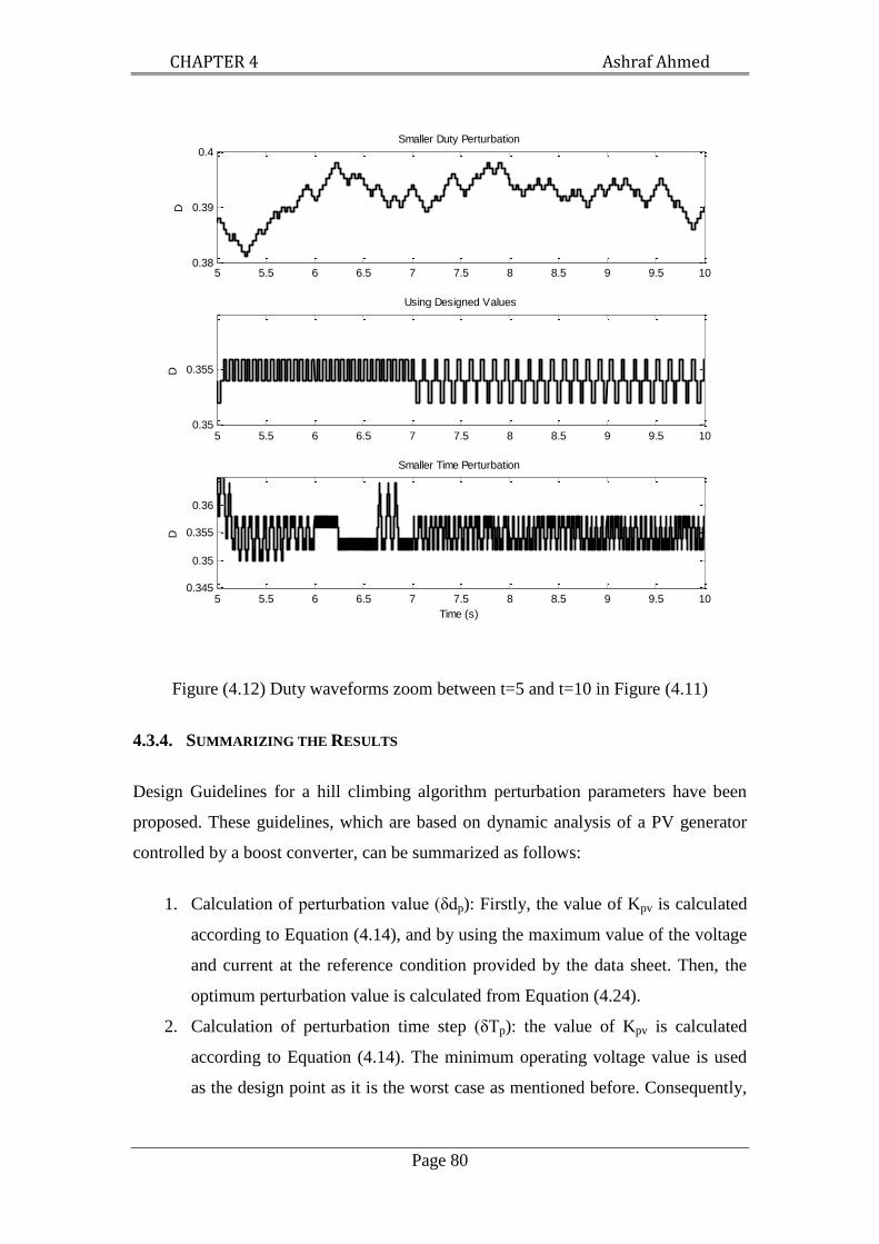
CHAPTER 4 Ashraf Ahmed
Page 80
Figure (4.12) Duty waveforms zoom between t=5 and t=10 in Figure (4.11)
4.3.4. SUMMARIZING THE RESULTS
Design Guidelines for a hill climbing algorithm perturbation parameters have been
proposed. These guidelines, which are based on dynamic analysis of a PV generator
controlled by a boost converter, can be summarized as follows:
1. Calculation of perturbation value (δdp): Firstly, the value of Kpv is calculated
according to Equation (4.14), and by using the maximum value of the voltage
and current at the reference condition provided by the data sheet. Then, the
optimum perturbation value is calculated from Equation (4.24).
2. Calculation of perturbation time step (δTp): the value of Kpv is calculated
according to Equation (4.14). The minimum operating voltage value is used
as the design point as it is the worst case as mentioned before. Consequently,
5 5.5 6 6.5 7 7.5 8 8.5 9 9.5 100.38
0.39
0.4
D
Smaller Duty Perturbation
5 5.5 6 6.5 7 7.5 8 8.5 9 9.5 100.35
0.355D
Using Designed Values
5 5.5 6 6.5 7 7.5 8 8.5 9 9.5 100.345
0.35
0.355
0.36
D
Time (s)
Smaller Time Perturbation

CHAPTER 4 Ashraf Ahmed
Page 81
Equation (4.23 or 4.25) is used to calculate the minimum perturbation time,
according to the availability of Cin in the circuit.
The V-I curves in the data sheet can be used to calculate (Kpv), which is used to
calculate the design parameters δdp and δTp. Figure (4.13) shows a V-I curve similar
to the data sheet curves. Point (a) is the design point for the parameter δTp. Kpv,
which can be found for this point by taking VPVa1, VPVa2 around (a), which refers to
points IPVa1, IPVa2, respectively, in the V-I curve. Kpv could be calculated from
The same equation can be used with point (b) (VPVb1, VPVb2, IPVb1 and IPVb2) to find
Kpv which is used in δdp design.
Figure (4.13) data sheet design of the perturbation parameters
4.4. PV CONTROL ALGORITHM WITH REDUCED POWER MODE
Direct duty ratio MPPT algorithms, as mentioned before in the literature are mainly
based on P&O methods. In this work, an MPPT controller was developed which is
based on variable step I.C. MPPT method. The algorithm has the following
advantages:
0 50 100 150 200 250 300 3500
2
4
Vpv
(V)
I pv (
A)
IPVa1IPVa2IPVb1IPVb2
b
VPVa1
VPVb2
VPVb1
a
VPVa2

CHAPTER 4 Ashraf Ahmed
Page 82
1. It is based on the I.C. MPPT method, which is faster in tracking the maximum
power than P&O and has a better dynamic performance under fast-changing
atmospheric conditions. Furthermore, I.C. MPPT causes less oscillation
around the maximum power point in the steady state, as it detects the
maximum power according to the incremental conductance sign.
2. Variable step size will produce faster MPPT at rapidly changing conditions.
The reason is that the duty ratio step size determines how fast the MPP is
tracked. Fast tracking can be achieved with bigger step size, but the system
will not operate at the MPP and will continuously oscillate around it. By
contrast, when using a small step size, the system will be slow. In both cases,
the tracking efficiency will be reduced. The variable step size method will
make a tradeoff between the two sides, where the step size will be large when
it is far away from the MPP, but will be small around the MPP, and
approaches zero on the MPP. Therefore, the system will rapidly track the MPP
and will not oscillate around it.
3. The proposed algorithm will also have the ability to work in a reduced power
mode. In this mode, the supervisory controller determines the power output
produced by the PV generator.
4. The proposed method is also very easy to be implemented in DSP.
In the following, the algorithm will be described and proved mathematically. Then, a
verification of the method by simulation will be proposed. A reduced power mode
will be added and simulation results will be presented.
4.4.1. VARIABLE STEP SIZE I.C. (V.S.I.C) METHOD
The incremental conductance method, one of the most widely used methods in the
field of MPPT control, is based on the fact that the slope of the PV array power with
respect to voltage is zero at the maximum power point, positive on the left of it, and
negative on the right (see Equation (4.26) ).
(4.26)
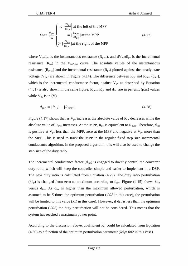
CHAPTER 4 Ashraf Ahmed
Page 83
(4.27)
where Vpv/Ipv is the instantaneous resistance (Rpvss), and dVpv/dIpv is the incremental
resistance (Rpv) in the Vpv-Ipv curve. The absolute values of the instantaneous
resistance (Rpvss) and the incremental resistance (Rpv) plotted against the steady state
voltage (Vpv) are shown in Figure (4.14). The difference between Rpv and Rpvss (dinc),
which is the incremental conductance factor, against Vpv as described by Equation
(4.31) is also shown in the same figure. Rpvss, Rpv and dinc are in per unit (p.u.) values
while Vpv is in (V).
(4.28)
Figure (4.17) shows that as Vpv increases the absolute value of Rpv decreases while the
absolute value of Rpvss increases. At the MPP, Rpv is equivalent to Rpvss. Therefore, dinc
is positive at Vpv less than the MPP, zero at the MPP and negative at Vpv more than
the MPP. This is used to track the MPP in the regular fixed step size incremental
conductance algorithm. In the proposed algorithm, this will also be used to change the
step size of the duty ratio.
The incremental conductance factor (dinc) is engaged to directly control the converter
duty ratio, which will keep the controller simple and easier to implement in a DSP.
The new duty ratio is calculated from Equation (4.29). The duty ratio perturbation
(δdp) is changed from zero to maximum according to dinc. Figure (4.15) shows δdp
versus dinc. As dinc is higher than the maximum allowed perturbation, which is
assumed to be 5 times the optimum perturbation (.002 in this case), the perturbation
will be limited to this value (.01 in this case). However, if dinc is less than the optimum
perturbation (.002) the duty perturbation will not be considered. This means that the
system has reached a maximum power point.
According to the discussion above, coefficient Kd could be calculated from Equation
(4.30) as a function of the optimum perturbation parameter (δdp=.002 in this case).

CHAPTER 4 Ashraf Ahmed
Page 84
(4.29)
(4.30)
where Vpva1 and Ipva1 is the voltage and current respectively in point (a), which was
shown in Figure (4.13).
Choosing the value of the maximum and minimum duty cycle perturbation is very
important in order to have a stable and smooth tracking. The step time between every
perturbation is constant at the optimum designed value (δTp), which can be calculated
from Equation (4.23). The designed value for this PV generator is .03 s. The control
algorithm is shown in Figure (4.16).
Figure (4.14) The basic idea for the V.S.I.S. method
160 180 200 220 240 260 280 300 320 340-0.8
-0.6
-0.4
-0.2
0
0.2
0.4
0.6
0.8
1
1.2
Vpv
(V)
R
pv (p.u.)
Rpvss
(p.u.)
d-inc (p.u.)
MPP
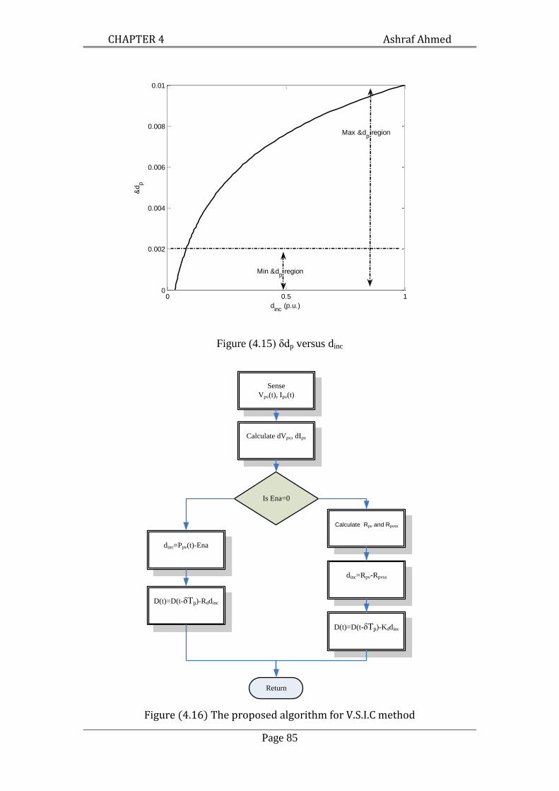
CHAPTER 4 Ashraf Ahmed
Page 85
Figure (4.15) δdp versus dinc
Is Ena=0
D(t)=D(t-δTp)-Kddinc
Return
Sense
Vpv(t), Ipv(t)
Calculate dVpv, dIpv
dinc=Rpv-Rpvss
dinc=Ppv(t)-Ena
D(t)=D(t-δTp)-Rddinc
Calculate Rpv and Rpvss
Figure (4.16) The proposed algorithm for V.S.I.C method
0 0.5 10
0.002
0.004
0.006
0.008
0.01
dinc
(p.u.)
&d
p
Min &dp region
Max &dp region

CHAPTER 4 Ashraf Ahmed
Page 86
4.4.2. THE REDUCED POWER MODE
There is a supervisory controller which states the operational modes of the system and
controls the power flow. Due to the following reasons, the supervisory controller may
need to reduce the output power from the PV generator. These reasons can be
summarized as follows:
1. The PV generator, due to high solar radiation or low temperature, can produce
more power than the system rated value [179]. The power electronics have a
rated value of power, but it is mainly slightly over rated. In spite of this, it will
not be enough if the solar radiation is increased to high values or the
temperature reduced to near zero oC. In winter both of these two conditions
can happen. These conditions can last for seconds, minutes and even hours.
This can be demonstrated by Figure (4.17), where the system has a rated
power of (950 W) in solar radiation (1000 W/m2) and cell temperature of (25
oC). The figure shows that when Tc is reduced to (0
oC) the power is increased
by (13.68 %) of the rated value, but when S is increased to (1200 W/m2), the
power is increased by (22 %). Furthermore, the power is increased by (39 %)
when S is increased to 1200 W/m2 and Tc is reduced to 0 oC. Consequently,
due to these conditions, the power has to be reduced around the rated values.
2. The wind generator output power can fluctuate more than the rated value due
to the high wind speed stalling control. If the inertia is high, the fluctuation
will be with a large time constant and it may also cause problems in the power
electronics.
3. In the standalone mode, the power demand by the load might be less than the
power produced by the generator, and the batteries are fully charged. The
supervisory controller can shut down the generator and use the battery energy
so the average power captured by the system will be reduced. Another solution
is to use dump load to absorb the extra power from the system. The best
solution is to reduce the output power from the PV generator, saving the
battery energy, and eliminating the need for dump resistance.

CHAPTER 4 Ashraf Ahmed
Page 87
Figure (4.17) Overrating levels of the PV output pwer with decreasing in temperature
and increasing in solar radiation.
The proposed reduced power mode is shown in Figure (4.16). The algorithm will
choose this mode according to signal (Ena) in the figure. If a non-zero signal (Ena) is
supplied from the supervisory controller the algorithm will drive the PV generator to
the reduced power mode. The perturbation value and direction is calculated in this
mode according to dinc as the MPPT mode. Equation (4.31) shows how dinc is
calculated.
(4.31)
As Ppv (t) is the measured power and Ena is the target power reference supplied by the
supervisory controller. The duty ratio can be calculated from Equation (4.32) where
Rd is a scaling factor that can be calculated from Equation (4.33). Quantity maximum
(dinc) is the maximum expected reduction in power, which can be considered the rated
value of the PV generator.
(4.35)
(4.33)
0 50 100 150 200 250 300 350 4000
200
400
600
800
1000
1200
1400
Vpv
(V)
Ppv (
W)
S=1000 W/m2 Tc=0 oC
S=1200 W/m2 Tc=0 oC
S=1000 W/m2 Tc=25 oC
S=1200 W/m2 Tc=25 oC
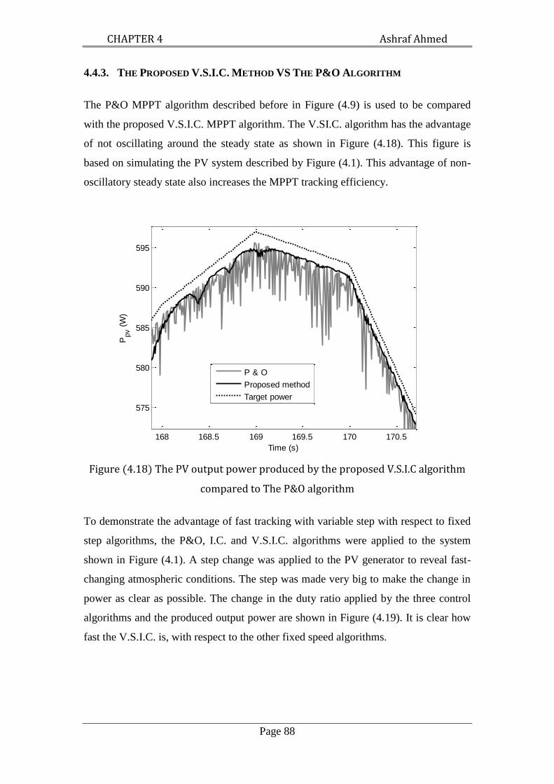
CHAPTER 4 Ashraf Ahmed
Page 88
4.4.3. THE PROPOSED V.S.I.C. METHOD VS THE P&O ALGORITHM
The P&O MPPT algorithm described before in Figure (4.9) is used to be compared
with the proposed V.S.I.C. MPPT algorithm. The V.SI.C. algorithm has the advantage
of not oscillating around the steady state as shown in Figure (4.18). This figure is
based on simulating the PV system described by Figure (4.1). This advantage of non-
oscillatory steady state also increases the MPPT tracking efficiency.
Figure (4.18) The PV output power produced by the proposed V.S.I.C algorithm
compared to The P&O algorithm
To demonstrate the advantage of fast tracking with variable step with respect to fixed
step algorithms, the P&O, I.C. and V.S.I.C. algorithms were applied to the system
shown in Figure (4.1). A step change was applied to the PV generator to reveal fast-
changing atmospheric conditions. The step was made very big to make the change in
power as clear as possible. The change in the duty ratio applied by the three control
algorithms and the produced output power are shown in Figure (4.19). It is clear how
fast the V.S.I.C. is, with respect to the other fixed speed algorithms.
168 168.5 169 169.5 170 170.5
575
580
585
590
595
Time (s)
Ppv (
W)
P & O
Proposed method
Target power

CHAPTER 4 Ashraf Ahmed
Page 89
Figure (4.19) The proposed V.S.I.C tracking speed compared to I.C. and P&O
4.4.4. DYNAMIC SIMULATION RESULTS
The simulation verification through real solar radiation (S) data is shown in Figure
(4.20). The data were collected at Durham University in rapidly changing weather
conditions to verify the ability of the MPPT algorithm in these conditions. The
ambient temperature is considered constant at 25 oC. The system shown in Figure
(4.1) was simulated using Matlab/Simulink with PLECS software. The PV generator
parameters are as proposed in Table (4.1).
The solar radiation is changing between 400 W/m2 and 900 W/m
2 in a time period of
215 s. The target power against the simulation output is shown in the Figure (4.20),
which shows that the target power is accurately tracked with a very small error. The
voltage (Vpv) in the output of the PV generator has some large changes as the solar
radiation changes rapidly, as shown between 40 s and 60 s in the time scale. This
happens because the algorithm provides the maximum duty ratio perturbation as the
3 3.5 4 4.5 5 5.5 6 6.5 70.25
0.3
0.35
0.4
0.45
D
3 3.5 4 4.5 5 5.5 6 6.5 7800
850
900
950
1000
1050
1100
Time (s)
Ppv (
W)
I.C.
V.S-I.C.
P&O

CHAPTER 4 Ashraf Ahmed
Page 90
operating point is rapidly moving away from the maximum power point. However,
from 0 s to 30 s and 70 s to 100 s, the changes in the solar radiation are slow, and so
the variation in Vpv is very small. In these cases, the slow change in solar radiation
makes a slow movement of the maximum power point and small duty ratio
perturbations (dinc). In many parts of the simulation, the variations are almost
terminated when the solar radiation is almost constant. This can be seen between 10 s
and 18 s in the time scale. The MPPT efficiency according to the rapidly changing
input simulation weather data is more than 99%.
The same system and part of the data used before (the first 100 seconds) is used to
verify the reduced power mode. As shown in Figure (4.21), between 20 s and 70 s, the
reduced (curtailed) power mode was applied. The controller drives the system
accurately into and out from the reduced power mode. Furthermore, whatever the
changes in solar radiation the power was kept constant at the target value.

CHAPTER 4 Ashraf Ahmed
Page 91
Figure (4.20) Dynamic simulation results verifyng the accuracy of the proposed
V.S.I.C.method in the MPPT mode of operation
0 20 40 60 80 100 120 140 160 180 200
600
800S
(W
/m2)
0 20 40 60 80 100 120 140 160 180 200
240
260
Vpv (
V)
0 20 40 60 80 100 120 140 160 180 200
2
3
I pv (
A)
0 20 40 60 80 100 120 140 160 180 200
200
400
600
800
Time (s)
Ppv (
W)
Target power
Simolation output

CHAPTER 4 Ashraf Ahmed
Page 92
Figure (4.21) Dynamic simulation results verifyng the accuracy of the proposed
V.S.I.C. method in the reduced power mode of operation
0 20 40 60 80 100
600
800S
(W
/m2)
0 20 40 60 80 100
240
260
280
300
Vpv (
V)
0 20 40 60 80 1001.5
2
2.5
3
3.5
I pv (
A)
0 20 40 60 80 100
400
600
800
Time (s)
Ppv (
W)
MPPT
Reduced power mode
CHAPTER 4 Ashraf Ahmed
Page 93
4.5. EXPERIMENTAL VERIFICATION
The PV controller proposed in this study is simple and easy to implement.
Furthermore, it deals with two operational modes: MPPT and reduced power modes.
The two algorithms are based on variable step perturbations of the duty ratio, which
increases the tracking speed and efficiency. To verify the control algorithm, a
laboratory test is carried out and Figure (4.22) shows a picture of the test rig setup. A
simplified block diagram, Figure (4.23), outlines the hardware arrangement.
An Agielnt-E4350B solar simulator is used to emulate the PV generator. A single
module described in Table (4.1) is simulated by the solar simulator to illustrate the
control method. The solar simulator was remotely controlled from a laptop computer
as shown in Figure (4.22). The control and data acquisition are implemented using a
desktop computer hosting a dSPACE real time control system which can be
programmed in the Matlab/Simulink environment [172]. The system and the control
parameters are the same as those used in simulation.
Figure (4.24) shows the experimental results as the characteristics of the PV simulator
were changed from (solar radiation=500 W/m2, 40
oC) at (time=41 s) to (solar
radiation=1000 W/m2, 25
oC), and then the characteristics were changed back again to
the last values at (time=91 s). The output results demonstrated that the proposed
control algorithm tracks the maximum power points with accurate and fast response.
In the figure, the measured power tracks the target power which is the maximum
power according to the solar radiation and temperature conditions.
To verify the V.S.I.C method speed, it was compared to the fixed regular I.C. as
illustrated in Figure (4.25). As shown in the figure, the duty ratio reaches a point
around the optimum value very fast in the proposed method in comparison with the
ordinary method.
The experimental verification of the reduced power mode is shown in Figure (4.26).
First, the controller was in MPPT mode under (solar radiation=1000 W/m2 and 25
oC
temperature). Then, the reduced power mode was applied at (time=41 s) with a
constant target power (Ppv=50 W). At (time= 83 s), the MPPT mode was applied to

CHAPTER 4 Ashraf Ahmed
Page 94
the system. The results show that: the proposed controller accurately works in the
reduced power mode as the output power was kept in the target value.
Dc/dc converter
Agielnt-E4350B
solar simulator
Remote controller
dSPACE unit
Load
Figure (4.22) Laboratory test rig
Desktop Computer
PV generator controller
Cw
A
V Load
Boost converter
DS
11
03
inte
rfac
e
IGB
T
gat
e d
riv
er
MA
TL
AB
-
SIM
UL
INK
-
Dsp
ace
vw
iw
Boost control
signal
The Solar Simulator
AGILENT-E4350B
Solar Simulator
Remote controller
Figure (4.23) Arrangement of laboratory system

CHAPTER 4 Ashraf Ahmed
Page 95
Figure (4.24) Experimental results for MPPT mode of operation as the solar radiation
and temperature change from (1000 W/m2 and 25
oC) to (500 W/m
2 and 40
oC)
respectively
0 20 40 60 80 100 12010
15
20
25
Time (s)
Vpv (
V)
0 20 40 60 80 100 1201
2
3
4
Time (s)
I pv (
A)
0 20 40 60 80 100 12020
40
60
80
Time (s)
Ppv (
W)
Measured power
Target power

CHAPTER 4 Ashraf Ahmed
Page 96
Figure (4.25) Proposed V.S.I.C control against fixed step I.C.
47.4 47.6 47.8 48 48.2 48.4 48.6 48.8 49 49.20.15
0.2
0.25
0.3
0.35
0.4
Time (s)
Duty
ratio
94.5 95 95.5 96 96.50.15
0.2
0.25
0.3
0.35
0.4
Time (s)
Duty
ratio
Variable step
Fixed step
(a)
(b)
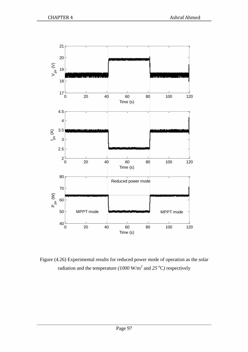
CHAPTER 4 Ashraf Ahmed
Page 97
Figure (4.26) Experimental results for reduced power mode of operation as the solar
radiation and the temperature (1000 W/m2 and 25
oC) respectively
0 20 40 60 80 100 12017
18
19
20
21
Time (s)
Vpv (
V)
0 20 40 60 80 100 1202
2.5
3
3.5
4
4.5
Time (s)
I pv (
A)
0 20 40 60 80 100 12040
50
60
70
80
Time (s)
Ppv (
W)
MPPT modeMPPT mode
Reduced power mode

CHAPTER (5)
INVERTER CONTROL
5.1. INTRODUCTION
As the market for small-scale renewable energy systems is rapidly increasing, the
need for power electronic converters also increases. The inverter is necessary in the
system to produce a sinusoidal wave to supply the ac load or connect to the grid. The
dc/ac single phase inverters are used to interface the sources with the single-phase
grid. The single-phase H-bridge inverter is a simple circuit topology with a small
number of components. Furthermore, it is simple to control but has one disadvantage
as manifested in the dc injection problem.
The proposed system in this study can be connected to the utility grid; therefore there
are quality standards for such aspects as low THD, elimination of the dc component
injected into the grid and active and reactive power control. The IEEE-929 standard
permits a limit of 5% for the THD in the output current, with individual limits of 4%
for each odd harmonic from 3rd
to 9th
and 2% from 11th
to 15th
. However, the dc
injection is limited to 0.5% of the rated output current. The European IEC61727
suggests similar standards with dc injection limits less than 1%. The dc current
injection in England is limited to 20 mA, which is less than .1% for the proposed
inverter. Other standards in the world have fewer restrictions and are easier to cope
with. In this study, the work will focus on fulfilling these strictest standards. The
proposed system is shown in Figure (5.1), where an H-bridge inverter interfaces a
renewable energy source with the grid. The dc renewable energy source is modelled
as a dc voltage source.
In this work, a small-scale H-bridge inverter is proposed to supply the power from the
renewable sources on the dc side to the grid or to the ac load. In Section (5.2), a peak

CHAPTER 5 Ashraf Ahmed
Page 99
current controller (p.c.c.) is proposed first for PWM and output current control. Then,
a grid connected control method is proposed in Section (5.3), based on the newly
developed standalone mode control. This is also based on p.c.c., which is described in
Section (5.2), to reduce the overall complexity of the system controller. The
simulation at the end of this section demonstrates the method. At the end of this
chapter, Section (5.4) suggests a method to remove the dc component of the inverter
output current with simulation and experimental verifications.
CdcV
Lf1
P.c.c.
V
vinvV
vg
Lf2 Lg
Cf
AA
Idc iinv
Vdc
Lf
PI Vdcr++
+-
vg
PLL
GainIdc
iinv Vdc
vg
Figure (5.1) Grid-connected H-bridge inverter control and circuit
5.2. THE PEAK CURRENT CONTROL METHOD
As mentioned before in Chapter (2); applying PI controller is very common with
small-scale inverters. However this kind of controller has relatively poor performance
due to the steady state error with tracking the sinusoidal reference. Furthermore, this
controller is unable to reject the noise in the current signal. With hysterias controllers,
there would be high bandwidth of harmonic spectrum. The other solution is to use
more complicated methods which need more analysis with faster DSPs.
A peak current control (p.c.c.) algorithm will be developed and modified to meet the
international standards for the current wave quality. The following section develops a
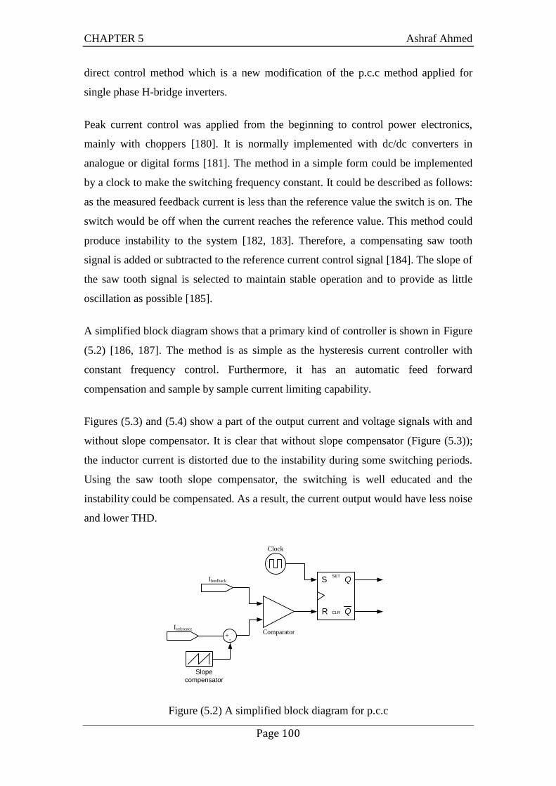
CHAPTER 5 Ashraf Ahmed
Page 100
direct control method which is a new modification of the p.c.c method applied for
single phase H-bridge inverters.
Peak current control was applied from the beginning to control power electronics,
mainly with choppers [180]. It is normally implemented with dc/dc converters in
analogue or digital forms [181]. The method in a simple form could be implemented
by a clock to make the switching frequency constant. It could be described as follows:
as the measured feedback current is less than the reference value the switch is on. The
switch would be off when the current reaches the reference value. This method could
produce instability to the system [182, 183]. Therefore, a compensating saw tooth
signal is added or subtracted to the reference current control signal [184]. The slope of
the saw tooth signal is selected to maintain stable operation and to provide as little
oscillation as possible [185].
A simplified block diagram shows that a primary kind of controller is shown in Figure
(5.2) [186, 187]. The method is as simple as the hysteresis current controller with
constant frequency control. Furthermore, it has an automatic feed forward
compensation and sample by sample current limiting capability.
Figures (5.3) and (5.4) show a part of the output current and voltage signals with and
without slope compensator. It is clear that without slope compensator (Figure (5.3));
the inductor current is distorted due to the instability during some switching periods.
Using the saw tooth slope compensator, the switching is well educated and the
instability could be compensated. As a result, the current output would have less noise
and lower THD.
Q
QSET
CLR
S
R
Ireference
+-
Ifeedback
Clock
Comparator
Slope
compensator
Figure (5.2) A simplified block diagram for p.c.c

CHAPTER 5 Ashraf Ahmed
Page 101
Figure (5.3) Inductor (Lf) current and output voltage waveforms without slope
compensation
Figure (5.4) Inductor (Lf) current and output voltage waveforms with slope
compensation
1.2865 1.287 1.2875
8
10
12
i g
(A)
Time (s)
1.2865 1.287 1.28750
100
200
300
400
Time (s)
v inv
(V)
1.2865 1.287 1.28758
9
10
11
12
13
i g
(A)
Time (s)
1.2865 1.287 1.28750
100
200
300
400
v g
(V)
Time (s)

CHAPTER 5 Ashraf Ahmed
Page 102
To design the slope value, which will compensate for the instability of the p.c.c., the
circuit shown in Figure (5.4) can be analysed using simplified differential equations.
All the elements in the circuit are considered ideal with L-filter (Lf). Furthermore, the
dc voltage control is considered stable and fast, so the dc side is assumed to be a
constant voltage source. For a unipolar switching pattern, there will be two modes of
operation, the first mode with the dc voltage source connected and the other with the
dc voltage disconnected, as shown in Figure (5.5).
Vdc
Lf ig
Mode (1)
vg
Mode (2)
Lf ig
vg
Figure (5.5) H-bridge inverter modes of operation with unipolar PWM
The inductor current, which is the inverter output current, is plotted for a single
switching period Ts. The rising current edge during mode (1) has a slope value of m1,
and the falling current edge has a slope value of m2. The compensating slope value
will be assigned with the symbol mc. These slopes are shown in Figure (5.6).
Figure (5.6) m1, m2 and mc in a one period of the inductor current
For mode (1):
(5.1)
Fore mode (2):
Time
i g
mc
m2
m1

CHAPTER 5 Ashraf Ahmed
Page 103
(5.2)
Equations (5.1) and (5.2) are only applicable for the first half of the sine wave, but the
result is applicable for the whole sine. Using the results in references [188-191], the
compensation ramp added for stable current loop can be found from the following
equation:
(5.3)
Using Equations (5.1), (5.2) & (5.3), then:
(5.4)
Therefore, vg in Equation (5.4) varies with time as it is a sine wave. Therefore, to
assure stability of the p.c.c.:
– (5.5)
(5.6)
From the last equation, it can be easy to design the compensating slope (mc).
The proposed unipolar modified p.c.c strategy is shown in Figure (5.7). The method is
the same as the one described before in Figure (5.2). Two S-R flip-flops are used to
switch the four switches of the inverter. A slope compensator is added to the reference
current (Ireference) and compared to the feedback signal (Ifeedback) to switch on IGBTs (1,
3). To switch IGBTs (2, 4), the slope compensator is subtracted from the reference
current and compared to the feedback current. The output voltage produced by this
switching orientation is unipolar.
The system shown in Figure (5.1) was simulated using Matlab/Simulink with the
PLECS software. At this stage, only the L-filter (Lf with the dash line) is used in the
simulation process. The forward voltage and on-state resistances were taken into
account with the H-bridge inverter IGBTs. The applied switching frequency is 10 kHz
with a 2 kW inverter rating. The output voltage and current and their THD are shown
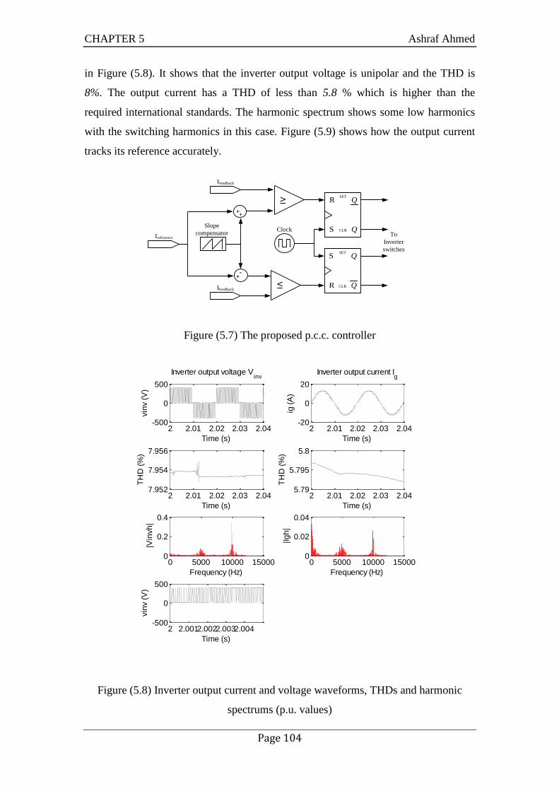
CHAPTER 5 Ashraf Ahmed
Page 104
in Figure (5.8). It shows that the inverter output voltage is unipolar and the THD is
8%. The output current has a THD of less than 5.8 % which is higher than the
required international standards. The harmonic spectrum shows some low harmonics
with the switching harmonics in this case. Figure (5.9) shows how the output current
tracks its reference accurately.
To
Inverter
switches
Q
Q
SET
CLRS
R
Ireference
++
Ifeedback
Slope
compensator
Q
QSET
CLR
S
R
+
Ifeedback
Clock
-
≥
≤
Figure (5.7) The proposed p.c.c. controller
Figure (5.8) Inverter output current and voltage waveforms, THDs and harmonic
spectrums (p.u. values)
2 2.01 2.02 2.03 2.04-500
0
500
Time (s)
vin
v (
V)
Inverter output voltage Vinv
2 2.01 2.02 2.03 2.047.952
7.954
7.956
Time (s)
TH
D (
%)
2 2.01 2.02 2.03 2.04-20
0
20
Time (s)
ig (
A)
Inverter output current Ig
2 2.01 2.02 2.03 2.045.79
5.795
5.8
Time (s)
TH
D (
%)
0 5000 10000 150000
0.2
0.4
Frequency (Hz)
|Vin
vh
|
0 5000 10000 150000
0.02
0.04
Frequency (Hz)
|Ig
h|
2 2.0012.0022.0032.004-500
0
500
Time (s)
vin
v (
V)

CHAPTER 5 Ashraf Ahmed
Page 105
Figure (5.9) ig versus iref with L-filter
5.2.1. LCL-FILTER
Due to the grid inverter’s switching operation, high frequency harmonics are
produced, which could cause trouble to the power system. A line filter is needed in the
inverter output in order to remove or reduce the harmonics to meet the standard
values. Passive line filters are normally used as L or LCL filters. The LC filter is not
desired with grid-connected inverters, as the resonance frequency of the filter would
be largely affected with the grid inductance [192]. To choose between L and LCL
filters, Figure (5.10) shows the frequency response of both filters. The figure was
plotted using values of (5 mH) for the L filter and (3 mH, 3µF, 1.5 mH) for the LCL
filter. The transfer functions used for L and LCL filters are as follows in Equations
(5.7) and (5.8) respectively. The two filters were chosen to have nearly the same
attenuation below the resonance frequency.
(5.7)
(5.8)
The figure shows that as the frequency is more than the resonance frequency, the
LCL-filter has more attenuation compared to the L-filter. The following advantages
can be concluded for the LCL filter [193-195]:
1. The voltage drop would be less as (Lf1+Lf2 < Lf) for the same harmonic
attenuation.
1.96 1.98 2 2.02 2.04-15
-10
-5
0
5
10
15
i g &
ire
f
(A)
Time (s)
iref
(A))
ig (A)

CHAPTER 5 Ashraf Ahmed
Page 106
2. The power factor control range would be higher.
3. The total cost of the filter would be less.
4. The size of the filter would be less.
Figure (5.10) The L-filter versus the LCL-filter
The LCL-filter design is not an easy task as many research papers were heading
towards this direction. Due to the notch around the resonance frequency, this filter
may cause instability problem and it needs to be designed carefully. A detailed design
procedure taking into account the system stability is not considered in this study.
Following the results of these references [196], the values of the filter can be found
through the following equations:
(5.9)
(5.10)
Cbase is the base capacitor for the system. According to these equations, the values of 3
mH, 3 µF and 1.5 mH were considered to Lf1, Cf and Lf2 respectively.
-100
-50
0
50
100
150
Magnitude (
dB
)
102
103
104
-270
-225
-180
-135
-90
Phase (
deg)
Bode Diagram
Frequency (Hz)
For L filter
For LC filter

CHAPTER 5 Ashraf Ahmed
Page 107
The system shown in Figure (5.1) was simulated in this stage with the LCL-filter
only. The results of the simulation are shown in Figure (5.13) compared to the results
that were proposed before in Figure (5.8); it is obvious that the current output of the
LCL-filter has better THD. The measured THD is 3.4% in case of the LCL-filter,
while it is 5.8% in the case of the L-filter. The LCL-filter case complies with the limit
imposed by the IEEE 929 standard, which is 5%. Figure (5.12) also shows that the
current smoothly tracks the reference values with different current values. In spite of
this result, the 3rd
harmonic is still relatively high, around 4% of the fundamental
component, which is on the edge of the international standards. Increasing the
switching frequency, for example, to 12 kHz, would largely reduce the THD. This
would keep the p.c.c. controller in the simple form. However, this would increase the
switching losses. Another way is to implement a selective harmonic elimination
technique for further THD reduction, keeping the switching frequency to 10 kHz. This
kind of technique can be implemented because there is a limited number of harmonics
with p.c.c., compared to other techniques such as hysteresis current control. In the
following subsection, the selective harmonic elimination will be proposed.
5.2.2. SELECTIVE HARMONIC ELIMINATION
In a hysteresis controller, the ripple frequency bandwidth occupies a high range while
the p.c.c. ripple bandwidth is limited to the low odd harmonics as the 3rd
, 5th
, and 7th
.
This would make selective harmonic elimination easily implemented in the p.c.c.
case. Figure (5.13) shows the p.c.c with selective harmonic elimination. A PIS
regulator was applied, as the one described In the letrature (Chapter 2), to eliminate
the specified harmonics.
The results of the simulation with and without applying selective harmonic
elimination are shown in Figure (5.14). The figure shows that before applying
selective harmonic elimination there are high 3rd
, 5th
and 7th
harmonics, and the THD
is 3.4%. After the application of selective harmonics elimination, the 3rd
, 5th
and 7th
are nearly eliminated while the THD is reduced to less than 1%. These results apply
for the rating current of the inverter. The selective harmonics elimination is very
effective in this case.

CHAPTER 5 Ashraf Ahmed
Page 108
Figure (5.11) Current output and THD using LCL-filter compared to L-filter,
Figure (5.12) The proposed method tracking performance with LCL-filter.
2.96 2.98 3-15
-10
-5
0
5
10
15
Time (s)
i g (
A)
L filter
2.96 2.98 30
2
4
6
8
10
Time (s)
TH
D (
%)
2.96 2.98 3-15
-10
-5
0
5
10
15
Time (s)
i g (
A)
LCL filter
2.96 2.98 30
2
4
6
8
10
Time (s)
TH
D (
%)
1.96 1.97 1.98 1.99 2 2.01 2.02 2.03 2.04-15
-10
-5
0
5
10
15
i g a
nd i
ref
(A)
Time (s)
iref
(A)
ig (A)

CHAPTER 5 Ashraf Ahmed
Page 109
To
Inverter
switches
Q
Q
SET
CLRS
R
Ireference
Ifeedback
Slope
compensator
Q
QSET
CLR
S
RIfeedback
Clock
≥
≤
++
++
+-
Ifeedback
Ireferance
PIS
3rd
h
PIS
5th
h
PIS
7th
h
+++
Unipolar p.c.c.
Harmonic elimination
+-
Figure (5.13) The proposed p.c.c. method with selective harmonic elimination
Figure (5.14) Harmonic spectrum and THD with and without selective harmonic
elimination
0 1000 2000 30000
0.1
0.2
0.3
0.4
Before applying selective
harmonic elimination
Frequency (Hz)
|I gh(f
)| (
A)
1.96 1.97 1.98 1.99 20
1
2
3
4
5
Time (s)
TH
D (
%)
0 1000 2000 30000
0.1
0.2
0.3
0.4
After applying selective
harmonic elimination
Frequency (Hz)
|I gh(f
)| (
A)
1.96 1.97 1.98 1.99 20
1
2
3
4
5
Time (s)
TH
D (
%)
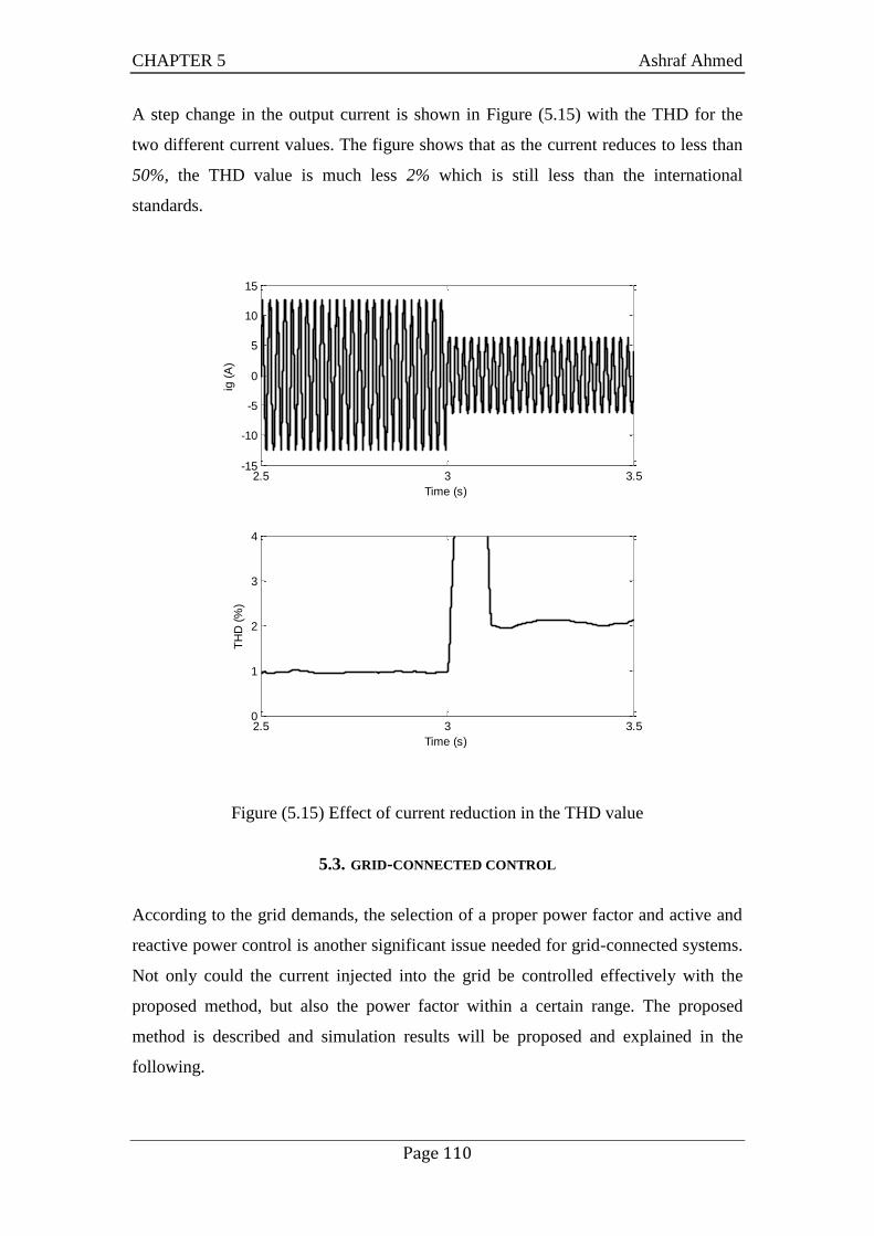
CHAPTER 5 Ashraf Ahmed
Page 110
A step change in the output current is shown in Figure (5.15) with the THD for the
two different current values. The figure shows that as the current reduces to less than
50%, the THD value is much less 2% which is still less than the international
standards.
Figure (5.15) Effect of current reduction in the THD value
5.3. GRID-CONNECTED CONTROL
According to the grid demands, the selection of a proper power factor and active and
reactive power control is another significant issue needed for grid-connected systems.
Not only could the current injected into the grid be controlled effectively with the
proposed method, but also the power factor within a certain range. The proposed
method is described and simulation results will be proposed and explained in the
following.
2.5 3 3.5-15
-10
-5
0
5
10
15
Time (s)
ig (
A)
2.5 3 3.50
1
2
3
4
Time (s)
TH
D (
%)

CHAPTER 5 Ashraf Ahmed
Page 111
For multi-source inverters, the objective of control is to control the active and reactive
power keeping the dc link voltage constant. Figure (5.16) shows a block diagram
describing the proposed active and reactive power control method. The method is
simple and easy to implement with small-scale renewable energy systems. The ac
reference current is calculated from the dc power side. Equation (5.11) shows the
equation used to calculate the ac reference current (Iinvr). In this work, the power
factor will be considered unity and the inverter efficiency (ηinv) is considered constant.
A simplified method to calculate the root mean square (r.m.s) value (Vg) from the ac
value (vg) is shown in Figure (5.17).
(5.11)
PI
P.c.c.
Vdcr
++
+-
Dc/ac
inverter
vg Idc
iinv
Vdc
sin (wt)
iinvr
×
×
PLL
Pdc
iinvVdc
g
dcinv
V
P
Vg
Calculation
Figure (5.16) A simplified block diagram for the active-reactive power control
method
-1
++
Filter
Vg
Calculation
22
vg Vg
Figure (5.17) A simplified method for r.m.s value calculation

CHAPTER 5 Ashraf Ahmed
Page 112
To design the PI dc-link voltage controller, the grid voltage magnitude is considered
to be constant. Furthermore, the inverter works with a unity power factor and as a
result, there is no phase shift between the voltage and current of the grid. According to
Figure (5.1), the grid power (Pg), the dc side power (Pdc) and the dc link capacitor
power (Pc) could be described by Equations (5.12), (5.13) and (5.14) respectively. The
three equations are related by Equation (5.15)
(5.12)
(5.13)
(5.14)
(5.15)
From these equations, a simplified dc link control loop, shown in Figure (5.18), has
been produced to design the PI controller. The Matlab/ control toolbox software has
been used to design values for Kp and Ki. A typical value for Kp and Ki are -0.2 and
0.1 respectively. These values were used to run the simulation of the system in Figure
(5.1). The results of the simulation with changing the power values are shown in
Figure (5.19). It shows that; the dc link voltage (Vdc) is controlled to track the
constant reference values with acceptable starting response. As the output power (Pg)
was changed by changing the input dc (Idc) in Figure (5.1), Vdc was kept at the
reference value Vdcr.
dcsC
1++
+- ÷Vg
Kp
Ig Pg
Idc
s
K i
+-
Vdc
Vdcr
Vdc
Vdc
Figure (5.18) The simplified dc link loop controller for the inverter

CHAPTER 5 Ashraf Ahmed
Page 113
Figure (5.19) Dc link voltage controller with step change in active power
The dc voltage and power factor controllers were tested by simulation according to
three conditions: active power change, two quadrant operations, and the variable
power factor. The simulation tests were carried out on Simulink/Matlab with PLECS
software. The system shown in Figure (5.1) was simulated as the reference value of
the dc voltage (Vdc) was kept at 400 V. The simulation results are summarized as
follows:
Active power change: Figure (5.20) shows Idc, ig, Vdc, Pg and Qg with different active
power values. The power factor is kept at unity in this test. The results show that; with
step changes in the input dc (Idc), the dc voltage is still constant at the reference value
(400 V). Furthermore, the VAR (Qg) is still near to zero and the power factor is kept
almost unity. This test clears the ability of the proposed controller to perform in
different power levels.
Two quadrant operations: In Figure (5.21), the system tested in two quadrant
operation as the grid power (Pg) reduced to be negative. This means the power was
extracted from the grid to the dc side. This mode is very important when batteries in
the dc side need to be charged. This is normally needed during the starting of the
0 1 2 3 41000
2000
Time (s)
Pg (
W)
0 1 2 3 40
100
200
300
400
500
Time (s)
Vdc &
Vdcr
(V)

CHAPTER 5 Ashraf Ahmed
Page 114
proposed system when the batteries were totally discharged before. This mode could
also be used; if there is a dc load, which needs to be supplied, and the energy sources
cannot provide this demand. The figure shows that even with the power extracted
from the grid to the dc side, the dc voltage is still constant at its reference value.
Furthermore, the power factor is nearly in its required unity value.
Variable power factors: The VAR (Qg) reference was varied in this simulation with
the results as shown in Figure (5.22). The power factor changed from lead to lag as
shown in the figure and the active power was kept constant. The figure also shows
that the dc voltage and the power factor controllers were working accurately.
Figure (5.20) Grid-connected control with active power step change
0 1 2 3 4 5 6
2
4
6
Time (s)
I dc (
A)
0 1 2 3 4 5 6-15
-5
5
15
i g (
A)
Time (s)
0 1 2 3 4 5 6350
400
450
Time (s)
Vdc (
V)
0 1 2 3 4 5 60
1000
2000
Time (s)
Pg (
W)
0 1 2 3 4 5 6-1000
0
1000
Time (s)
Qg (
VA
R)

CHAPTER 5 Ashraf Ahmed
Page 115
Figure (5.21) Grid-connected control with two quadrant operation
0 1 2 3 4 5 6-5
0
5
Time (s)
I dc (
A)
0 1 2 3 4 5 6
-10
0
10
i g (
A)
Time (s)
0 1 2 3 4 5 6350
400
450
Time (s)
Vdc (
V)
0 1 2 3 4 5 6
-10000
10002000
Time (s)
Pg (
W)
0 1 2 3 4 5 6-500
0
500
Time (s)
Qg (
VA
R)

CHAPTER 5 Ashraf Ahmed
Page 116
Figure (5.22) Grid-connected control with change in p.f.
5.4. STANDALONE MODE CONTROL
In this study, the proposed standalone control mode is based on the p.c.c. method,
which is described early in this chapter. The inverter output current is controlled from
the dereference current provided by the voltage control loop, as shown in Figure
(5.23). An extra output filter (Cfo) is needed for better performance within this mode
of operation. A value of 10 µF was found to give a good performance and lower THD.
The ac voltage control loop is controlled using a PIS controller. The dc link voltage
in this case is maintained constant by energy storage connected to the same dc link.
0 0.5 1 1.5 2 2.5 3 3.5 4
-20
0
20
Time (s)
p.f
. angle
(o)
0 0.5 1 1.5 2 2.5 3 3.5 4
Time (s)
Vdc (
V)
0 0.5 1 1.5 2 2.5 3 3.5 40
1000
2000
Time (s)
Pg (
W)
0 0.5 1 1.5 2 2.5 3 3.5 4-1000
0
1000
Time (s)
Qg (
VA
R)

CHAPTER 5 Ashraf Ahmed
Page 117
The load current is controlled using an instantaneous direct current control method
(p.c.c.) that will guarantee fast transient response, reduced total harmonic distortion
(THD), and higher disturbance rejection. Furthermore, the method is simple and easy
to implement. There is no need for harmonic elimination to be used within this mode
as it is observed that, with the simple form of the p.c.c method, satisfactory current
and voltage waveforms are produced.
Lf1
P.c.c.
V
vinvV
vg
Lf2
Cf
A
iinv
VdcLoad
A
ig
PIS vgr+-
iinvvg
Cfo
Figure (5.23) standalone mode control and circuit
The system shown in Figure (5.23) was simulated in Matlab/Simulink with PLECS
software. The dc side was considered a dc voltage source as the dc link was controlled
by the battery bank side controller. The output voltage (vg) against the reference
voltage (vgr) is shown in Figure (5.24).The figure shows that the voltage output tracks
the reference value in an efficient way. The output voltage and current waveforms
with their THD values is shown in Figure (5.25), and the value shown is for rated load
conditions. The THD for both wave forms according to the simulation is less than 2.8
%, which is a very interesting value compared to the simplicity of the proposed
control method.
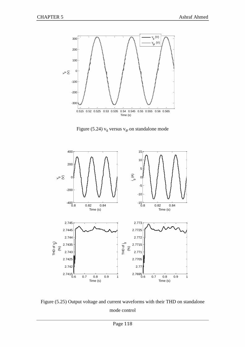
CHAPTER 5 Ashraf Ahmed
Page 118
Figure (5.24) vg versus vgr on standalone mode
Figure (5.25) Output voltage and current waveforms with their THD on standalone
mode control
0.515 0.52 0.525 0.53 0.535 0.54 0.545 0.55 0.555 0.56 0.565
-300
-200
-100
0
100
200
300
v g
(V)
Time (s)
vg (V)
vgr
(V)
0.8 0.82 0.84-400
-200
0
200
400
Time (s)
v g
(V)
0.6 0.7 0.8 0.9 12.7415
2.742
2.7425
2.743
2.7435
2.744
2.7445
2.745
Time (s)
TH
D o
f v g
)
(%)
0.8 0.82 0.84-15
-10
-5
0
5
10
15
i g (
A)
Time (s)
0.6 0.7 0.8 0.9 12.7695
2.77
2.7705
2.771
2.7715
2.772
2.7725
2.773
Time (s)
TH
D o
f i g
(%)

CHAPTER 5 Ashraf Ahmed
Page 119
To test the transient performance of the controller under load change, the load was
simulated as a variable resistor in the output of the inverter. The reference value of the
ac voltage (vg) is a sine wave with r.m.s value of 220 V. The results of the simulation
are exposed in Figure (5.26), which shows the output current (ig), the output power
(Pg), the output voltage (vg) and the r.m.s. value of the output voltage. The figure
shows that a step change was applied to the load from rated value 2kW to less than .8
kW at t=1.08 in the time scale. In spite of the step change, the controller effectively
keeps the voltage at the reference value with negligible transients. The proposed p.c.c
controller is the same one used before with the grid connection control mode, and this
will reduce the overall system control complexity.
Figure (5.26) Standalone mode control simulation results
0 0.5 1 1.5 2-20
0
20
i g (
A)
Time (s)
0 0.5 1 1.5 20
1000
2000
3000
Time (s)
Pg (
W)
0 0.5 1 1.5 2-500
0
500
Time (s)
Vg (
V)
0 0.5 1 1.5 20
100
200
300
Time (s)
R.m
.s o
f V
g
(V)
CHAPTER 5 Ashraf Ahmed
Page 120
5.5. DC INJECTION ELIMINATION
The work described in this section is concerned with the risk of dc injection into the
network from the small-scale single-phase inverters without output transformers. Due
to an approximate short circuit characteristic of an ac network, a little dc voltage
component, which can accidently be produced by the inverter, will produce large dc
injection. This causes detrimental effects on the network components, particularly the
network transformers which can saturate, resulting in irritant tripping. This may also
increase the losses in and reduce the lifetime of the transformers, if not tripped.
Moreover, the existence of the dc component can induce metering errors and
malfunction of protection relays. There are thus stringent regulations in many
countries to prevent the network from large dc injection. This thesis presents a new
method of complying with such a requirement by an inverter that does not have a
network side output transformer.
5.5.1. THE PROPOSED CONTROL STRATEGY
This study proposes a new method of measuring the dc component in the inverter
output current. The output current is measured by a resistive shunt and the obtained
voltage signal is processed by a specially designed and tuned analogue filter to
increase the signal-noise ratio so that the dc level, as specified in standards, e.g. .5%
of the rated inverter current, becomes measurable. The response is adequately fast
even for renewable energy systems which are normally working under variable
conditions. This work explains the design of the filter circuit and the use of it in a
closed loop control system aiming to keep the dc injection low – below the standard
limit. System performance is illustrated by simulation and experimental results. The
study focuses on a full bridge voltage source inverter operating in a unipolar PWM
mode. The block diagram of the transformerless inverter under study is depicted in
Figure (5.27) showing the control for dc injection compensation.

CHAPTER 5 Ashraf Ahmed
Page 121
CdcV vg
L
Rm
DC filter
Amplification
DC voltage,
frequency & power
factor controller
Renewable
energy
equivalent DC
source
PI
P.c.c.
IGBT
Gate
Driver
V
iinv
vg
Vdc
Modulation
index
vinv
Vdc
Isolation
+
+
V
iinv
Figure (5.27) The grid-connected inverter circuit and control
5.5.2. CAUSES OF DC INJECTION
There are three main factors which can cause dc injection into the network from a
single-phase H-bridge voltage source inverter. These are
-Unequal semiconductor device characteristics in the inverter, including on-state
resistance and on-state forward saturation voltage, and the temperature coefficients of
these parameters. The device characteristics are affected by inevitable variations
during fabrication and packaging and can also drift in operation due to degradation
mechanisms such as bond wire lift-off. The circuit in Figure (5.27) was built in
Matlab/Simulink with PLECS software, and the simulation was performed assuming
that the on-state voltage of the IGBT devices in the inverter is unbalanced by 0.05 V.
Figure (5.28) shows the imbalance produced by the on-state voltages. A part of the
positive cycle shows that the forward voltages in this leg of the inverter are the same.
In the negative half-cycle, one of the IGBTs has less forward voltage by .05 V. For a
typical 230 V single-phase feeder, the series resistance in the Thévenin equivalent
circuit representation would be 0.01 to 0.04 . For a modulation index of 0.8 in the

CHAPTER 5 Ashraf Ahmed
Page 122
inverter and 1 kW output power at unity power factor, the simulation showed that the
dc injection was between 375 mA and 1500 mA. This shows how difficult it is to
comply with the typical standard requirement of the dc injection being less than e.g.
20 mA, in this case of 1 kW inverter. The only way is probably to set the dc under
close-loop control if a low frequency output transformer is to be avoided, which
however depends on how accurately the weak signal of a small dc can be measured.
Figure (5.28) Effect of unbalance in forward IGBT voltages
- Dc bias that can be included in the inverter PWM switching process. This is
particularly vulnerable to the blanking time between the upper and lower switches in
the same leg of the bridge. Simulation shows that the dc injection in the range of
hundreds of mA can be easily reached with unbalance of blanking time in a few
microseconds between the positive and negative half cycles of the inverter output.
- Dc bias of the output current sensor, which also could provide dc bias to the PWM
process. This will cause imbalance between the positive and negative half-cycles and
causes dc component to be injected.
-5
0
5
Time (s)
A p
art
of
v inv (
V)
wave
Unbalance in V
f
between the IGBTs
Positive half
cycle Negative half
cycle
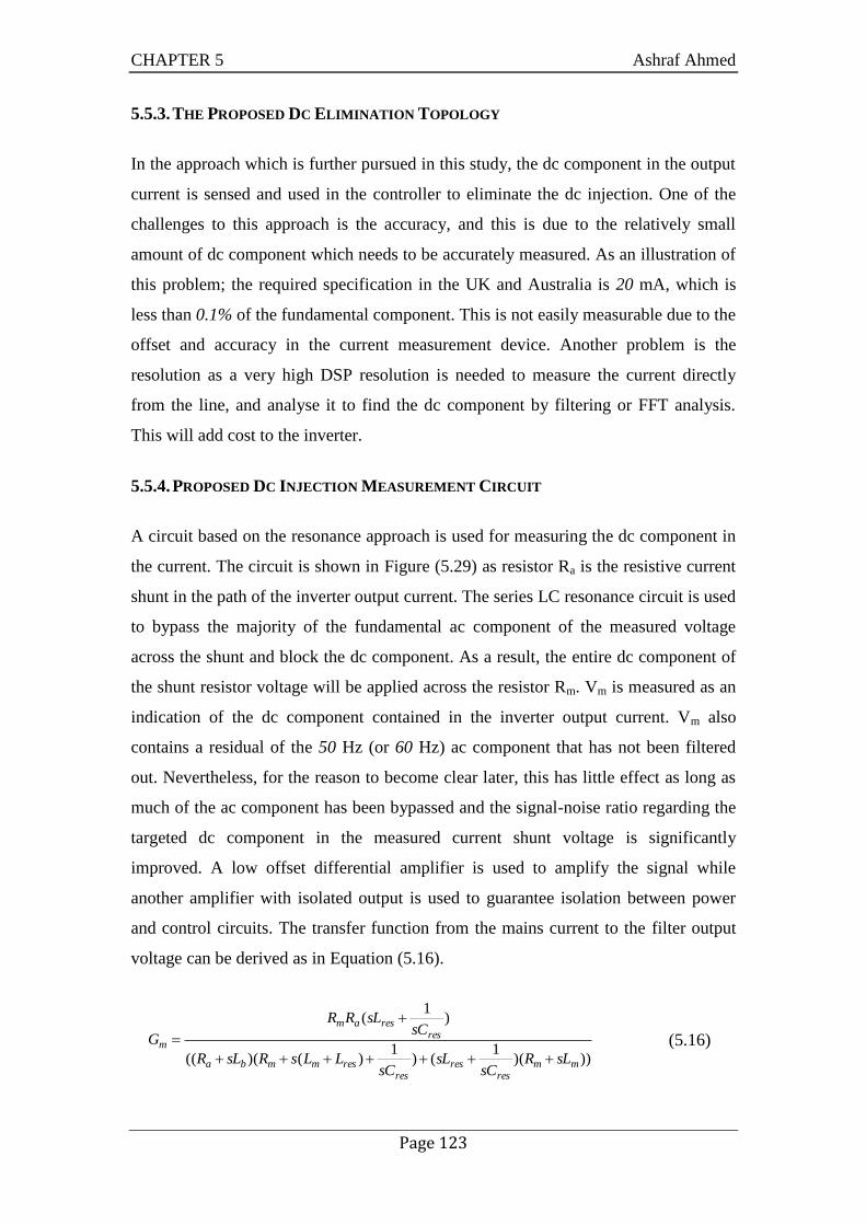
CHAPTER 5 Ashraf Ahmed
Page 123
5.5.3. THE PROPOSED DC ELIMINATION TOPOLOGY
In the approach which is further pursued in this study, the dc component in the output
current is sensed and used in the controller to eliminate the dc injection. One of the
challenges to this approach is the accuracy, and this is due to the relatively small
amount of dc component which needs to be accurately measured. As an illustration of
this problem; the required specification in the UK and Australia is 20 mA, which is
less than 0.1% of the fundamental component. This is not easily measurable due to the
offset and accuracy in the current measurement device. Another problem is the
resolution as a very high DSP resolution is needed to measure the current directly
from the line, and analyse it to find the dc component by filtering or FFT analysis.
This will add cost to the inverter.
5.5.4. PROPOSED DC INJECTION MEASUREMENT CIRCUIT
A circuit based on the resonance approach is used for measuring the dc component in
the current. The circuit is shown in Figure (5.29) as resistor Ra is the resistive current
shunt in the path of the inverter output current. The series LC resonance circuit is used
to bypass the majority of the fundamental ac component of the measured voltage
across the shunt and block the dc component. As a result, the entire dc component of
the shunt resistor voltage will be applied across the resistor Rm. Vm is measured as an
indication of the dc component contained in the inverter output current. Vm also
contains a residual of the 50 Hz (or 60 Hz) ac component that has not been filtered
out. Nevertheless, for the reason to become clear later, this has little effect as long as
much of the ac component has been bypassed and the signal-noise ratio regarding the
targeted dc component in the measured current shunt voltage is significantly
improved. A low offset differential amplifier is used to amplify the signal while
another amplifier with isolated output is used to guarantee isolation between power
and control circuits. The transfer function from the mains current to the filter output
voltage can be derived as in Equation (5.16).
)))(1
()1
)()(((
)1
(
mmres
resres
resmmba
resresam
m
sLRsC
sLsC
LLsRsLR
sCsLRR
G
(5.16)

CHAPTER 5 Ashraf Ahmed
Page 124
Ra
Lb
Cres
Lres
Lm
Rm
imain
vmR1
R1 Ro
R2
R2
Vo
+
-
Figure (5.29) dc injection measurement circuit
5.5.5. CHOOSING MEASURING CIRCUIT COMPONENTS
In this section, design of the values of the filter component will be chosen. There are
three components need to be chosen in the circuit, which is Lb, Lm, and Rm, and the
resonance circuit filters. These components can be designed as follows:
-The value of the inductance Lb is chosen according to the filter rating where Lb
blocks the mains ac current component and it is a short circuit to the dc component. Lb
can be chosen according to
b
mainab
I
IRL
(5.17)
where (ω) is the mains frequency (rad/s), Ib is the ac current through Lb and Imain is the
inverter output rated current.
-The value of inductance Lm is chosen to give some tolerance in Lres and Cres in the
series resonant branch.

CHAPTER 5 Ashraf Ahmed
Page 125
-To choose the precise value for the resistance Rm, consider the steady state transfer
functions from the dc or fundamental ac component in the inverter output current to
the corresponding components in Vm (Equation (5.16)). The ac and dc gains had been
plotted against the resistance (Rm) as shown in Figure (5.30). The Figure shows that as
Rm increases both the dc and ac gains of the filter increase. However, the increase of
the dc gain saturates as Rm approaches 10 Ω. Furthermore, the ac gain attenuates the
fundamental component of the main current by values from less than 0.5% to 2%
while the dc gain attenuates the dc by values less than 20% to more than 80%. This
shows how the proposed circuit makes the percentage of the dc component to the ac
component increase from less than .2%, which is not measurable, to more than 15%.
Taking into account the maximum input value for the amplifier, the tolerance in the
passive filter components (Lres and Cres), and the amplifier offset value, the value of
Rm can be chosen. In our design case, a value of 3 Ω has been applied.
Figure (5.30) Choosing filter output resistance Rm
-To show how to design the resonance components values of Lres and Cres, a value of
Lres was chosen with changing Cres in Equation (5.16). Figure (5.31) shows the ac gain
against the capacitor values in farad with and without resonance circuit. It is obvious
that the minimum ac gain occurs in the resonance case, but because of the tolerance in
the capacitor and inductor values, the capacitors are designed to be 20% more than the
resonance values. The reason for this is to avoid the sharp increase in the ac gain less
0 1 2 3 4 5 6 7 8 9 100
0.005
0.01
0.015
0.02
AC
Ga
in
0 1 2 3 4 5 6 7 8 9 100
0.2
0.4
0.6
0.8
1
DC
Ga
in
Resistance (ohm)

CHAPTER 5 Ashraf Ahmed
Page 126
than the resonance value. The ac gain in the figure is attenuated to less than 25% in
the designed point while the dc gain is not affected.
5.5.6. CONTROLLER DESIGN
To simplify the system model, the causes of dc injection are collectively represented
as a dc voltage source at the inverter output (Vs) as shown in Figure (5.32).
Furthermore, the compensating voltage produced by off-setting the modulation index
(Mdc) of the inverter is considered a controllable dc voltage source (Vc). The inverter
control will also respond to the residual fundamental ac component in Vm. However,
the response is small compared to the normal inverter output voltage. The grid
exhibits series inductance (Lf) and resistance (Rf).
Figure (5.31) Choosing resonance filter components
Lres Cres
Ra
RmLm
Vm
Lb
Mdc
Lf Rf
Vc
Vs
Figure (5.32) Circuit simplifications for analysis of the dc
1.6 1.8 2 2.2 2.4 2.6 2.8 3
x 10-4
0
0.005
0.01
0.015
0.02
0.025
0.03
0.035
0.04
Cres
(F)
AC
Gain
Without resonance circuit
Resonance point
Design point

CHAPTER 5 Ashraf Ahmed
Page 127
The transfer function from the inverter output voltage to the current is:
s
ss
sT
KG
1 (5.18)
where fs RK /1 , ffs RLT / . The transfer function of the measurement circuit was
proposed before in Equation (5.16). The block diagram of the closed-loop control
system is shown in Figure (5.33) where a PI controller is used to control the dc
component of the current by off-setting the modulation index of the inverter. In the
design of the controller, disturbance rejection and noise suppression were taken into
account. The Matlab control toolbox is used to design the system controller. The
designed root locus and the open loop bode plot of the system are shown in Figure
(5.34). The figure shows that the system is designed to show as faster response as
possible without high peaks in the dc component.
Vm_ref
PI Gs GmVc
VmVs
Figure (5.33) Controller block diagram for the dc component equivalent circuit
Figure (5.34) Bode and root locus diagrams of the inverter according to the dc
component of the current
-800 -600 -400 -200 0-600
-400
-200
0
200
400
600
Real Axis10
110
210
310
410
5-180
-135
-90
P.M.: 57.9 deg
Freq: 445 rad/sec
Frequency (rad/sec)
-80
-60
-40
-20
0
20
40
G.M.: Inf
Freq: Inf
Stable loop
CHAPTER 5 Ashraf Ahmed
Page 128
5.5.7. SIMULATION RESULTS
The time-domain simulation was carried out using Matlab/ Simulink for a simplified
system configuration as shown in Figure (5.27). The dc link is a controlled voltage
source emulating the renewable energy source supplying a single-phase grid-
connected H-bridge inverter. The dc link voltage is maintained to be constant at 400 V
and the inverter is controlled to supply the grid with 2 kW power with unity power
factor. Unequal on-state state voltages between the inverter arms are adjusted to
produce a dc of 20 mA injected into the grid while the dc elimination controller is
applied at t=1 s from the start of the simulation. The simulation results are shown in
Figure (5.35), which illustrates the mains current (Imain), the mains dc component
(Imain-DC), the filter output (Vm), and the dc component in the filter output voltage (Vm-
DC). This simulation results demonstrate that the dc can be eliminated by the controller
and this proves the controller design based on a simplified method. Furthermore, the
filter increases the signal-noise ratio of the dc component in Vm with respect to the
residual ac component which is regarded as noise. The dc component in Vm becomes
measurable after amplification. To demonstrate this, the dc component in the mains
current is less than 0.2% while it is more than 5% in the output of the filter,
corresponding to a 25 times improvement of the signal-noise ratio.
5.5.8. EXPERIMENTAL VERIFICATION
A block diagram of the experimental test rig setup is shown in Figure (5.36)Error!
Reference source not found. where a dc voltage source is connected to the H-bridge
inverter, which supplies a passive load. To artificially cause a dc component in the
inverter output current, a circuit of variable resistance connected to a diode is
paralleled to the load resistance as shown in Figure (5.36). The controller for the dc
injection elimination and the inner loop for the inverter PWM process are
programmed in Matlab/Simulink and implemented using an embedded dSPACE real
time control system [172]. The filter output is measured as shown in the figure and
provided to the controller where the H-bridge inverter PWM control signals are
generated. The dc injection elimination control is applied after 18 seconds from the
start of the experiment.

CHAPTER 5 Ashraf Ahmed
Page 129
Figure (5.35) Time-domain simulation results
The experimental results are shown in Figure (5.37) and Figure (5.38) where the data
were collected on a digital scope and dSPACE respectively. Figure (5.37) shows the
inverter output current before dc component elimination, which contains a dc
component. Figure (5.38) shows the output voltage of the measuring filter circuit Vm.
The variable resistance was adjusted to produce almost 12.3 mA dc component in the
inverter output current whose fundamental ac component is approximately 1.06 A, as
shown in Figure (5.37). It is clearly shown in Figure (5.38) that the controller
eliminates the dc component to a non-significant level. Furthermore, the test results
show that as the inverter output current changes, the controller keeps the dc-injected
current at the same level, which remains to be insignificant. This is particularly useful
in renewable energy systems where the input power is always fluctuating. This
0.6 0.8 1 1.2 1.4 1.6 1.8 2-20
0
20
I ma
in (
A)
0.6 0.8 1 1.2 1.4 1.6 1.8 2
-0.04
-0.02
0
I ma
in-D
C (
A)
0.6 0.8 1 1.2 1.4 1.6 1.8 2-2
-1
0
1
Vm
(V
)
0.6 0.8 1 1.2 1.4 1.6 1.8 2
-0.04
-0.02
0
Vm
-DC
(V
)
Time (s)

CHAPTER 5 Ashraf Ahmed
Page 130
experimental results show a slight divergence from the expected ideal characteristics
and this is due to the tolerance of the passive filter component values. With this, the
filter can still adequately sense the dc component in the inverter output current. As a
demonstration, the dc component is only 0.8% in the inverter output current, while it
is almost 13% in the filter output voltage signal. Consequently, the objective of the
research has been achieved.
Cdc
L
Rm
DC filter
Amplification
DC voltage
source
IGBT
Gate Driver
V
Isolation
Desktop Computer
DC injection elimination
controller
DS1103
interface
Vd
c
Mea
sured
sig
na
l
MA
TL
AB
-
Sim
ulin
k-
Dsp
ace
Rdc
RL
D
Figure (5.36) The experimental test rig Configuration
Figure (5.37) Measured inverter output current when the dc component was
applied, its value is shown in the right side of the figure (-12.3 mA)
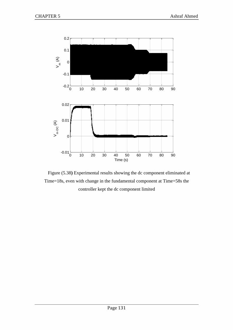
CHAPTER 5 Ashraf Ahmed
Page 131
Figure (5.38) Experimental results showing the dc component eliminated at
Time=18s, even with change in the fundamental component at Time=58s the
controller kept the dc component limited
0 10 20 30 40 50 60 70 80 90-0.2
-0.1
0
0.1
0.2
Vm
(A
)
0 10 20 30 40 50 60 70 80 90-0.01
0
0.01
0.02
Vm
-DC
(A
)
Time (s)

CHAPTER (6)
SUPERVISORY CONTROL
6.1. INTRODUCTION
Under different operating conditions, the power generating system can provide a
desired quality of operation with power electronics and control processing units. Such
a system is considered a hybrid power system, as it combines various electrical energy
sources and energy storage, and contains both continuous and discrete signals.
Renewable energy systems with batteries are an illustration of such hybrid energy
systems. Supervisory control is essential to manage the power between the different
components of a renewable energy system. Furthermore, it supervises and regulates
the operations of the local controller for every component of the system in the various
operating modes. Standalone systems with renewable energy resources are hard to
control due to changing and unpredictable generator output.
Energy storage devices would smooth the power output and provide greater
availability of the system. If the renewable energy system is connected to the utility
grid, it increases the control difficulty. This happens because the system needs the
capability to work in both modes, i.e. with and without grid connection. Furthermore,
the number of operational modes will increase and the control problem will be
complicated.
A supervisory controller, which manages the operation of the hybrid PV-Wind unit
with a storage system in standalone and grid-connected modes, will be proposed in
this chapter. The local controllers were designed and verified for the different system
components in the previous chapters. The supervisory controller is then needed to
provide a smooth operation through the different modes of the system. During the
operational modes, this controller also has to be able to keep the system’s power
quality within the specified constraints. The advantage of modularity, which adapts

CHAPTER 6 Ashraf Ahmed
Page 133
the controller to work with different system configurations with no or very little
change, has to be considered with the supervisory controller. Therefore, the proposed
control can supervise a PV-Wind hybrid or a single-sourced renewable energy
generating system. Furthermore, it can work with standalone or grid-connected
systems.
In this chapter, the system configuration and local controls will be summarized in
Section (6.2). This is followed by explaining the proposed supervisory controller in
Section (6.3). The simulation results will demonstrate the control strategy in the end
of this chapter.
6.2. SYSTEM CONFIGURATION AND CONTROL
With reference to Figure (6.1), the PV and wind generators produce electrical power
which is extracted from the solar and the wind energies respectively. The related
symbols are shown in Table (6.1) below. The system configuration and control of all
the involved system components will be described in the following subsections:
6.2.1. WIND GENERATOR SIDE CONTROL
The ac output power of the wind generator is rectified by a diode rectifier and
controlled by a boost converter. The boost converter provides MPPT at low and
moderate wind velocities while it limits the power and rotor speed by stalling the
generator at high wind velocities. The details of the controller design, simulation
results and experimental verification were explained above in Chapter (3). A braking
resistor is used to switch off the wind generator according to a control signal from the
supervisory controller.
6.2.2. PV GENERATOR SIDE CONTROL
The PV generator is a nonlinear dc source which is controlled by a dc/dc boost
converter. This converter provides MPPT to the PV generator using the method
described above in chapter (4). The reduced power operation (RPO) is also provided
to limit the generated power from the system according to the following scenarios:

CHAPTER 6 Ashraf Ahmed
Page 134
1. If the generated power is higher than the power electronics ratings. The reason
is that the power generated from the PV generator can largely increase above
the data sheet rating with temperature reduction. Furthermore, solar radiation
can increase to high limits on certain summer days, which increases the power
output over the ratings. This was fully discussed in Chapter (4).
2. If the system is on the standalone mode and the battery bank is fully charged,
in order to reduce the renewable energy generator disconnection periods. A
full discussion of this operational mode will be explained later in this chapter.
6.2.3. BATTERY BANK SIDE CONTROL
The battery storage devices can be used in a wide range of applications due to their
fast response and silent operation. Recently, due to the increased application, the
battery storage technologies have significantly improved. The batteries are used in
many applications, such as power system frequency control, which helps to improve
the stability and availability of power systems [196]. Using battery storage systems as
a short-term home backup is also affordable [197]. Another very promising
application is the integration with isolated or grid-connected renewable energy
systems, which will be proposed in this system. The battery storage is very important
to provide a smooth output power and to increase the overall availability of the
system. In the following sub-sections, the battery bank model and the control strategy
are proposed.
A. BATTERY BANK MODEL
A simplified battery bank model is proposed in this stage [198]. The electromotive
force (Ebatt) is modelled as a controlled voltage source, which is calculated as a
function of the SOC (Csoc) (Equation (6.1)). The SOC is calculated according to the
discharging / charging current Equations (6.2, 6.3) respectively.
CDSOCCDCCbattEC)EE(E (6.1)
0socdisch
cap
disch
disch_SOCCdtI
C3600C
(6.2)
0socch
cap
ch
ch_SOCCdtI
C3600C
(6.3)

CHAPTER 6 Ashraf Ahmed
Page 135
PV Generator
PMSG
wm
Wind speed
dc/dc
Converter
dc/dc
Converter
Rectifier
Inverter
Wind
Generator
Dc bus
Batteries
Bank
Solar
radiation
LOAD
P2
LOAD
P3
LOAD
P1
Braking
W G
Controller
Inverter
Controller
Charger
Controller
Utility
Grid
Ipv
Iw
Brake
Controller
Vw
Vdc
Ibatt
vinv
iinv
vgig
Vpv
Ppv
Pw
SOC
I.T.
PL
Ppvr
S.M
B.M
PV.M
W.M
L.M
PV G
Controller
L.P2.M
L.P3.M
S.R.M
Ibattr
L.P1.M
L.P2.M
L.P3.M
B.M
S.MS.M
PV.M
W.M Ibattr
Vdc
Rst
S.R.M
Cdc
Starting
Circuit
Δf
ΔVdc
Supervisory
Controller
vgo
Figure (6.1) A block diagram for the proposed system

CHAPTER 6 Ashraf Ahmed
Page 136
Table (6.1) Description of the symbols in Figure (6.2)
Number Symbol Description
Inp
uts
1 Ppv PV generated power (p.u.)
2 Pw Wind generated power (p.u.)
3 SOC State of charge of the batteries (p.u.)
4 I.T. Islanding test
5 PL Load demand power (p.u.)
6 Δf The change in grid frequency
7 ΔVdc The change in dc voltage (Vdc)
Ou
tpu
ts
1 Ppvr Reduced mode reference PV power (p.u.)
2 S.M. System mode
3 B.M. Batteries mode
4 PV.M. PV generator mode
5 W.M. Wind generator mode
6 L.M. Load priority 1 mode
7 L.P2.M. Load priority 2 mode
8 L.P.M. Load priority 3 mode
9 S.R.M. Starting resistance mode
10 Ibattr Batteries reference current (p.u.)
The circuit is shown in Figure (6.2) as the battery output e.m.f (Ebatt) is considered to
increase linearly with the SOC (CSOC). The minimum value of (Ebatt) is the minimum
discharge voltage (ECD) and the maximum value (ECC) is the maximum charging
voltage. The steady state value of the SOC (Csoc0) is considered as input to the battery
model in the simulation process. The dynamic instant value is calculated inside the
model using Equations (6.2, 6.3) according to the charging and discharging currents.
The charging current is considered positive at charging mode and negative at
discharging mode. Practically, there are many methods to measure the SOC value, and
many methods are described in references [199-201]. A detailed SOC measurement
circuit is outside the scope of this work.

CHAPTER 6 Ashraf Ahmed
Page 137
Batteries
bank
DCh
PWM
PI
PI
PI
Supervisory control
signal
Ibattr
From the supervisory
controller
A
VCsoc0
PWMPI
PI
PI
Vdcr-1
-1
Cbatt
Lbatt
DDisch
I bat
t
Ibatt
Vd
c
Vd
c
Vd
c
Ibatt
Figure (6.2) Diagram for battery side with charge/discharge circuit and control
B. BATTERY POWER ELECTRONICS AND CONTROL
A dc/dc converter is used to control the batteries as shown in Figure (6.2). A boost
dc/dc converter works on the discharging mode while a buck dc/dc converter works
on the charging mode [202]. The battery controller can be divided into the following
modes of operation according to the supervisory control signal:
1. Standalone mode - the controller regulates the current to provide constant dc
bus bar voltage (Vdc). The starting mode is controlled in the same way as this
mode where the (Cdc) capacitor is charged using a starting resistor. The
starting circuit will be discussed in Section (6.3).
2. Grid-connected mode - the dc/dc converter is controlled to provide the
required reference dc current from the battery bank. The reference current is
calculated by the supervisory controller.
The supervisory controller provides the batteries’ current reference signal (Ibattr) (see
Figure (6.1)). If this signal is positive, the batteries will be charged by the buck
converter dc/dc converter. The boost converter would then be switched off. However,
if the (Ibattr) signal is negative, the batteries will be discharged by the boost converter

CHAPTER 6 Ashraf Ahmed
Page 138
and the buck circuit would be OFF. The batteries would be switched off if the
batteries’ current is zero. In the grid-connected mode, the batteries would not be
discharged to values less than (50%) of their capacity and would only be charged.
This will increase the life time of the batteries [203]. In the standalone mode,
discharging the batteries less than (20%) is acceptable under controlled
circumstances; while at less than (10%) the batteries will be charged only [204] by the
renewable energy generators. Therefore, the supervisory controller will manage the
batteries’ charging/discharging to provide a better performance. This will increase the
battery life and increase the system availability. The battery charging/discharging
currents are limited to the batteries and the charger circuit rating. More details on how
to deal with this problem will be discussed in Section (6.3).
6.2.4. INVERTER SIDE
The H-bridge single-phase inverter control is controlled as discussed before in
Chapter (5). The supervisory controller is used to switch between the grid-connected
and the standalone modes of operation, as shown in Figure (6.3). This inverter is
controlled to guarantee the following:
1. The dc bus voltage (Vdc) is constant.
2. The current and voltage waveforms are modulated to fulfil the international
standards. This is performed using a control process was discussed before in
Section (5) and summarized in Figure (6.3).
3. The load demand is fulfilled according to the supervisor control signals. Those
signals are directed to the inverter reference currents.
4. The supplied power is controlled to be in the required power factor, which is
unity in this case. This is performed by matching the reference current to the
grid voltage using PLL controller.
5. The injected dc current component to the grid is eliminated by using the
previously designed dc component measuring circuit.
6. The proposed system works properly during switching between different
modes of operation.
7. The islanding condition is detected and the supervisory controller is driving
the system accordingly [205].

CHAPTER 6 Ashraf Ahmed
Page 139
The islanding case is detected and a zero signal would be seen by the supervisory
controller, which will drive the system to the standalone operation. Once the grid was
available again, another on signal would be provided to the supervisory controller to
switch the grid on. The signal provided to the supervisory controller is called the
islanding test signal (I.T.) and Figure (6.4) assembles how the test calculated. There
are two signals compared by an (and) gate to provide the (I.T.) signal. The first signal
is the grid side voltage (vgo), which is measured after the grid switch as shown in
Figure (6.1). If vgo has a value (there is grid voltage), the switch output is (1), and if
this value is zero the output is (0). The second value is the islanding measurement
output signal which is (0) when the system is in standalone and (1) when the system is
connected to the grid. The inverter output voltage is controlled on the standalone
mode to provide constant output voltage. The dc voltage (Vdc) is controlled by the
battery controller, as discussed before.
6.2.5. LOAD SIDE
Demand side load management is an essential subject in the recent years. One of its
applications is to provide stability and security to the utility grid. Furthermore, it can
be used by utility grid end users to reduce prices for the electricity market [204]. In
this study, load management is performed to increase the total power captured by the
load and to reduce the renewable energy generators disconnections. This will increase
the overall availability of the system. The load management is needed when the
system cannot provide the full demand on the standalone mode of operation. The local
loads are given different priorities, according to the importance of every load. This
can be switched ON and OFF by the supervisory controller.
In the research in the present study, every local load will be assigned with a priority.
The loads will be switched ON and OFF according to the SOC of the batteries. A
detailed description of the load management process will be discussed in the
supervisory controller section. The loads are modelled in the simulation process as a
controlled resistor. The resistor value is determined according to the load profile, the
root mean square value of the load voltage and the power factor. The loads also have a
capacitor and an inductor to model the reactive part of the load.

CHAPTER 6 Ashraf Ahmed
Page 140
CdcV
vg
Lf1
V
vinv
V
vg
Lf2 Lg
Cf
AA
Idc iinv
Vdc
To
Inverter
switches
Q
Q
SET
CLRS
R
iinv
Slope
companestaor
Q
QSET
CLR
S
Riinv
Clock
≥
≤
++
+-
iinv
iref
PIS
3rd
h
PIS
5th
h
PIS
7th
h
+++
Unipolar p.c.c.
Harmonic elimination
+-
PIVdcr ++
+-
vg
PLL
iref
Gain
Idc
Vdc
From supervisory
controller
PIS
vgr
+-
vg
PIS
Grid-connected
controller
Standalone
controller
Dc component
elimination
+++
PI
Vm
Dc injection
measuringv
m
Renewable energy
sources
Figure (6.3) Control on the inverter side

CHAPTER 6 Ashraf Ahmed
Page 141
PLL
And
vgo
1
0
From Islanding circuit
I.T.
Figure (6.4) The islanding test (I.T.) signal calculation
6.3. THE SUPERVISORY CONTROLLER
The supervisory controller for hybrid power systems is a system wide controller
which supervises the modes of operation and manages the power flow in the power
system. One of the important controller rules is to guarantee smooth transition
between the different modes of operation. Furthermore, the supervisory controller also
sets the local controllers for the different components at the different modes of
operation in order to ensure their optimum operation. The supervisory controller could
be illustrated as shown in Figure (6.5).
Local Controllers
Supervisory Controller
Controlled Plant
Q
QSET
CLR
S
R
Measured signals
Inputs Outputs
Control
signals
Figure (6.5) Supervisory controller for a hybrid system
The hybrid power system modes are designed to provide system equilibrium
conditions. The system characteristics for these modes would be held in specific
constraints. Furthermore, the energy flow would be balanced between the system
components. The number and the assemblies of those operating modes are designed

CHAPTER 6 Ashraf Ahmed
Page 142
according to the system components and configurations. The proposed supervisory
controller controls the hybrid PV-wind-generated system with batteries storage. The
system can work in grid connection mode when the utility grid is available and in
standalone mode when the utility grid is unavailable. The proposed power
management strategy depends on the SOC of the battery storage and the utility grid
availability. The main objective of the power management strategy, including load
management, is to accomplish power balance between energy sources and loads on all
modes of operation. The supervisory controller is based on the following:
1. The system will always be connected to the grid if the grid is available or if
there is no fault.
2. The extra generated power to the load demands will be directly transferred to
the grid when the batteries are fully charged or when the batteries do not exist
in the system.
3. The load will draw power from the grid only if the power produced by the
energy sources and the storage is not sufficient for the load. This could happen
when the SOC of the batteries is lower than a specific value; then, the batteries
would not be discharged.
4. In the standalone mode, the batteries are always connected to provide balance
between the load and the renewable energy sources.
5. Load management will only be used in the standalone mode operation.
6. If the charge current is higher than the rating of the batteries or power
electronics, the system will be regulated to the reduced power mode.
7. If the discharge current is higher than the rating of batteries or power
electronics, the extra power would be supplied by the grid in the grid mode. In
the standalone mode, the system would use load management to overcome this
problem.
Therefore, the system has one starting mode and two main operating modes:
Starting mode
Standalone mode
Grid-connected mode

CHAPTER 6 Ashraf Ahmed
Page 143
The transitions between the modes of operations including the primary ones are
shown in Figure (6.6). As shown in the figure, the operating modes of the system can
be described in the following sub-sections.
S1 (NOM)S2 (RPM)
S3(LCM)
S4(DM)
Grid Operation
Standalone Operation
S0(SM)
Starting Mode
S5(DDM)
S6 (OCM)
G1 (NOM)G2 (RPM)
G3(LCM)
G4 (FCM)
Figure (6.6) Different modes for the renewable energy system
6.3.1. STARTING MODE (S0(SM))
The starting, or standby operation, is the process deployed when the Hybrid PV-Wind
generated system is switched on. It is the state S0(SM) on Figure (6.6) where all the
generators, loads and grid are disconnected. In the circuit shown in Figure (6.1),
where the supervisory controller tests the battery charge, and then switches on the
starting resistance with batteries and dc capacitor (Cdc). The starting resistance is
designed to reduce the high starting current when the storage element is connected to
the fully discharged dc capacitor (Cdc). If the starting resistor is not there, the batteries
will be shorted at the starting period and the battery charger circuit could not handle
the starting current. The starting resistor is chosen to limit the starting current within
the circuit rating. The starting resistor is applied for 1 s until the dc bus voltage
reaches the required dc bus voltage (i.e. 400 V). In the next stage, the PV generator,
wind generators, inverter and loads are switched on. In a very special case, the grid
could be used to charge the batteries. That might be needed if the batteries were fully

CHAPTER 6 Ashraf Ahmed
Page 144
discharged and the renewable energy sources are not producing much power.
Therefore, the batteries could be charged by the grid inverter. The capability of the
proposed inverter control to work in such a mode was discussed in chapter (5).
6.3.2. STANDALONE MODE
This operational mode is activated when the utility grid is not available. The
availability of the utility grid is detected according to the voltage and current sensors
in the input of the utility grid. On this mode, the battery bank is always connected to
the system. The dc link voltage (Vdc) is controlled directly by the battery bank side to
be kept constant (i.e. 400 V). Furthermore, the different states are dependent on the
battery state of operation. In the following, these operating states will be discussed.
A. NORMAL OPERATING MODE (S1(NOM))
This mode occurs when the SOC of the batteries, which, for the purpose of this study,
is considered between 0.5 p.u. and 0.9 p.u., is in the normal working region.
Furthermore, the PV and the wind generators are connected to the system normally
and the power produced according to the weather conditions. All the loads also
connected and the system is then capable to supply the full demand.
B. REDUCED-POWER MODE (S2(RPM))
The reduced power mode is needed when the power produced by the renewable
energy sources increases to values higher than the rated ones due to the reasons
discussed before in chapter (5). Furthermore, as the batteries are fully charged, i.e.
SOC is above 0.9 p.u., it is necessary to reduce the power supplied by the renewable
energy generators. This will keep the generators connected to the system, because the
other solution is then to disconnect the generators. The reduced power mode was
presented also in chapter (5).
C. LOW CHARGING MODE (S3(LCM))
The LCM will be considered as soon as the SOC of the batteries falls below 0.5 p.u..
To avoid the fast discharging of the batteries, the supervisory controller will then
switch off the lowest priority load (Load P3).

CHAPTER 6 Ashraf Ahmed
Page 145
D. DISCHARGE MODE (S4(DM))
If the SOC was decreased to a value below 0.3 p.u., the batteries would then be
discharged. This means more loads have to be disconnected to keep the system
working. The loads with the second priority (Load P2) added to Load P3 would be
switched off on the system.
E. DEEP DISCHARGE MODE (S5 (DDM))
As the batteries continue to discharge (i.e. SOC< 0.1 p.u.) and the renewable energy
generators is not able to supply the load, the supervisory controller will switch off all
the loads. This will protect the batteries from deep discharge. In this stage, the
renewable energy generators will only charge the batteries.
F. OVER -CHARGE MODE (S6 (OCM))
The OCM is the opposite of the DDM (i.e. SOC>= 0.95 p.u.), and then the renewable
energy generators is disconnected to protect battery bank over-charging. Therefore,
the batteries will only supply all the demands until the SOC is in the normal range
again.
6.3.3. GRID-CONNECTED MODE OF OPERATION
The grid will be connected when it is available. The batteries work as the backup
source on the normal operating mode while the grid will only be used in special cases,
which will be discussed later. The dc link voltage (Vdc) is controlled from the inverter
side. This means; the supervisory controller is working to reduce the power extracted
from the utility grid. That will reduce the overall cost of the system. The operating
states of the grid connected mode could be described in the following points.
A. NORMAL OPERATING MODE (G1(NOM))
As the utility grid is available and the batteries measure 0.9 p.u.>SOC >0.5 p.u., the
system would then work normally (G1(NOM)). In this mode, the renewable energy
generators are both connected and their operation depends on the weather conditions.
The battery bank would be charged if the generated power was more than the load

CHAPTER 6 Ashraf Ahmed
Page 146
demand, and it would be discharged if the generated power was insufficient to the
load demands.
B. REDUCED POWER MODE (G2(RPM))
When the utility grid is available, the RPM is applied only if the power produced is
more than the system rated value. The batteries work then is the same as the
G1(NOM) discussed in the previous section.
C. LOW CHARGING MODE (G3 (LCM))
If the SOC of the batteries is less than 0.5 p.u., the system becomes on LCM and the
batteries have to be disconnected. The utility grid works as a backup source for
supplying the extra load demand if the generated power is less than the load demands.
The generated extra-power will charge the batteries if it is more than load demand.
D. FULL CHARGE MODE (G4(FCM))
This mode is applied when the batteries are fully charged (i.e. SOC >0.9 p.u.). This
mode is the opposite of the G3(LMD) with respect to the battery operation. The
batteries would be discharged when the generated power less than the load demands.
In case of the generated power higher than the load demand, the extra-power will be
supplied to the grid.
6.3.4. THE SUPERVISORY CONTROLLER ALGORITHM
A simplified proposed algorithm is shown in Figure (6.7), while the inputs and
outputs of the algorithm are shown in Figure (6.1) and in Table (6.1). As the system
starts the supervisory, controller tests the batteries and then drives the system to the
starting mode (S0(SM)). The utility grid is tested and, if it is available, the controller
switches on the grid, or the controller drives the system to the standalone mode. In the
standalone mode, the secondary system modes are derived according to the SOC of
the batteries as shown in the algorithm. The grid availability is tested all the time and,
if it is available, the controller switches the system to the grid-connected mode. If the
power generated at any time is higher than the rating, the system enters the reduced
power mode. The batteries are always kept charged at least to 0.1 p.u. in any mode of

CHAPTER 6 Ashraf Ahmed
Page 147
operation; this protects them against deep discharging and keeps some charge for the
next starting up. All the inputs and constraints in the supervisory controller are in per
unit values. This will make the supervisory controller capable of supervising systems
with different system ratings. Furthermore, the controller will be capable of
supervising a single renewable energy source or multi-source systems. The modularity
of the supervisory controller will provide a wide range of renewable energy systems
which the controller can also supervise.
Start
Are the batteries
charged?
S0
Mode
Is dc voltage
Stable?
Connect
utility grid
Standalone
operation
Is the utility grid
available?
S2
(RPM)
SOC > 0.95 p.u. SOC > 0.9 p.u.
SOC < 0.1 p.u.
0.9 p.u.≥SOC ≥
0.5 p.u.
0.95 p.u.>SOC >
0.9 p.u.
0.5 p.u.>SOC ≥
0.3 p.u.
0.3 p.u.>SOC ≥
0.1 p.u.
Is the generated power in the
rating?
0.9 p.u.≥SOC ≥
0.5 p.u.
SOC < 0.5 p.u.
S1
(NOM)
S3
(LCM)
S4
(DM)
S5
(DDM)
G1
(NOP)
G3
(LCM)
G4
(FCM)
S6
(OCM)
Return
S2, G2
(RPM)
Figure (6.7) The algorithm of the supervisory controller

CHAPTER 6 Ashraf Ahmed
Page 148
6.4. SIMULATION RESULTS
The system shown in Figure (6.1) was modelled and simulated by dynamic simulation
using the Simulink/ Matlab with PLECS software. The supervisory controller was
programmed by conventional programming using an embedded Matlab function. The
system will run with dynamic measured input data of solar radiation and temperature.
The SOC will be changed to simulate how the supervisory controller will supervise
the system during the different modes of operation. This will demonstrate the ability
of the controller to manage the system operation. The wind generator is considered in
these results with very small inertia to speed up the starting operation and reduce the
simulation time. The inputs of the system, in this section, were changed to actual
measured solar radiation, wind velocity, and temperature data. The data was collected
at Durham University, and it is shown in Figure (6.8). The load demand was divided
as discussed before to three priorities
1- House load demand; it is considered at .75 kW.
2- Pump Load demand which was assumed as constant power load of .5 kW
3- Another constant load of .5 kW, which was considered as a heating system.
Every load from the three loads was assigned a priority. The house load was assigned
with the highest priority (P1 Load), the heating system with the second priority (P2
Load) and the Pump was assigned the lowest priority (P3 Load). According to the
given data, the system has been simulated. The results are shown in Figures (6.9),
(6.10), (6.11) and (6.12).
Figure (6.9) shows the supervisory controller output ON/OFF control signal. These
control signals are described before as shown in Figure (6.1). The power flow and the
SOC of the batteries are shown in Figure (6.10). The controlled power quality signals
are shown in Figure (6.11).The system modes were controlled according to system
mode signal (S.M.). This signal is 0 in the standalone mode at the first 85 s. However,
it is 1 in the grid mode during the rest of the simulation time. The results can be
discussed as follows:

CHAPTER 6 Ashraf Ahmed
Page 149
Figure (6.8) Simulation inputs: load demand profile (P1 Load), solar radiation, and
wind velocity, respectively
Starting Mode (S0(SM)) – (from 0 s to 1 s)
On this mode, the system was started by the batteries – as discussed before – only to
charge the dc link capacitors (Cdc). Figure (6.10) shows how the dc voltage (Vdc) is
building up at this time. At the end of this mode, the supervisory controller provided
signals to the PV and wind generators to start up. These are shown on the ON/OFF
signals of Figure (6.9) (also see Figure (6.1) and table (6.1)). According to the SOC of
the batteries, the load was also started by the load mode signal (L.M.).
Standalone mode-(from 1 s to 85 s)
The supervisory controller tested the availability of the grid after the starting up mode
(S0(SM)). The utility grid was found unavailable, and for (85 s) the system was
simulated on the standalone mode. The different operating states of the standalone
0 20 40 60 80 100 120 140400
600
800
1000
Sola
r ra
dia
tion
(W/m
2)
0 20 40 60 80 100 120 140
10
15
20
Time (s)
Win
d s
peed
(m/s
)

CHAPTER 6 Ashraf Ahmed
Page 150
mode were controlled according to the SOC which is shown in Figure (6.10). During
this time, the simulation output can be described as follows:
1. From 1 s to 20 s
The simulated SOC signal, between 1 s and 20 s, was 0.6 p.u. and 0.8 p.u.. Therefore,
the system was on the (S1(NOM)) mode of operation. During this mode, the
supervisory controller switched on all the loads and the generators while it switched
off the grid as shown in Figure (6.9). According to the solar radiation, temperature
and wind velocity, the PV and wind generators produced the power, as shown in
Figure (6.10). The load demand is also shown in the same figure. As the load demand
was higher than the generated power, the batteries current – as shown in Figure (6.10)
– was positive, which means that the batteries were discharged during this time. In
Figure (6.11), the dc voltage (Vdc) is kept at its designed value at 400 V. As the grid
was off, all the power was supplied by the inverter and the grid power was zero.
Furthermore, the reactive power was kept at zero value – as shown in the figure – to
maintain a unity power factor.
2. From 20 s to 30 s
During this time the system was on the (S2(RPM)) mode of operation as the SOC
measured 0.92 p.u., as shown in Figure (6.10). The total wind and PV generated
power was lower than the load demand, so the supervisory controller discharged the
batteries (the battery current was positive as in Figure (6.10)). Therefore, the system
works the same as the S1(NOM). If the generated power had been more, the
supervisory controller would have reduced the power generated to be equivalent to the
demand load.
3. From 30 s to 40 s
As the SOC measured more than 0.95 p.u., as shown in Figure (6.10), the system was
on the S6(OCM). On this mode of operation, the supervisory controller switches off
the wind and PV generators as shown in Figures (6.9) & (6.10). As a result, the load
was only supplied by the batteries.

CHAPTER 6 Ashraf Ahmed
Page 151
4. From 40 s to 60 s time scale
When the SOC was reduced to 0.4 p.u. and then to 0.3 p.u. (Figure (6.10), the system
was on the S3(LCM). In this mode, the supervisory controller again switched on the
PV and wind generator as shown in Figures (6.9) and (6.10). The load with the lowest
priority (P3 load) was switched off while the other load was kept on (Figure (6.9). By
looking at Figure (6.10), it can be seen that the batteries were charging and the battery
ban current was negative during this mode. This happened because the generated
power from the PV and wind generator was higher than the load power. The dc
voltage (Vdc) and the reactive power generated by the inverter were kept constant.
This can be observed in Figure (6.11).
5. From 60 s to 70 s
If the SOC is reduced to more than 0.2 p.u., as shown in Figure (6.10), the system
enters the S4DM. The supervisory controller switches off the load with the second
priority (P2 load) over the load with the third priority (P3 load), as shown in Figure
(6.9). As a result, more current would be directed to the batteries by the supervisory
controller (Figure (6.10)).
6. From 70 s to 80 s
The SOC reduced to 0.1 p.u., which was the S5(DDM). Consequently, the supervisory
controller switched off the whole demand (L.M.) as shown in Figure (6.9). The total
power generated by the renewable energy sources would be instantly directed to the
batteries. The dc voltage (Vdc) was also kept constant, which means that the capacitor
was kept charged.
7. From 80 s to 85 s
The SOC was increased again to 0.2 p.u. as shown in Figure (6.10). Therefore, the
whole demand was switched on again as shown in Figure (6.9) while the loads with
priorities (P3 load, P2 load) were switched off. The battery bank current (Figure
(6.10) was negative. This means it was charged during that time. Figure (6.9) shows
that the batteries were always connected. The grid power was always zero, as shown
in Figure (6.11); this means the grid was disconnected. The same figure shows that

CHAPTER 6 Ashraf Ahmed
Page 152
the dc voltage (Vdc) was kept constant during the whole standalone operation.
Furthermore, the reactive power that was generated by the converter is also always
zero. This means the power factor was kept constant during the entire stand-alone
operation. This figure demonstrates that the inverter controller was successful during
the standalone operation with different system modes and dynamic change of the
input weather conditions. The supervisory controller was also successful in managing
the power during the entire range of the standalone operation.
Grid mode (from 85 s to the end time scale)
At time (85 s), the grid was available so the supervisory controller detected that and
provided ON (S.M.) signal to switch on the grid. Therefore, the system is in the grid
mode. The dc voltage control is transferred from the batteries side to the inverter side
as explained before in Section (6.3). An over shoot happened in Vdc, during mode
transfer, and that is shown in Figure (6.11). The secondary modes of the grid-
connected mode during its operational time can be discussed as follows:
1. From 85 s to 100 s
The SOC was still measured as 0.2 p.u. and increased to 0.4 p.u., and hence the
system was on the G3(LCM). Therefore, the supervisory controller would stop the
batteries from discharging. The batteries were disconnected, as shown in Figure (6.9),
as the batteries’ mode signal (B.M.) was reassigned zero. This happened because the
power generated from the renewable energy sources was lower than the load power as
shown in Figure (6.10). As a result, the load drew power from the grid as shown in
Figure (6.11).
2. From 100 s to 120 s
As the SOC signal was increased to 0.6 p.u. and 0.8 p.u., the system was in the
G1(NOP). The batteries were switched on again (see Batteries mode signal in Figure
(6.9)). As the power generated was higher than the load power (see Figure (6.10)), the
batteries current was positive. The batteries were discharged during this time. All the
power was provided by the inverter – as shown in Figure (6.11) – and the grid power
was reduced again to zero.

CHAPTER 6 Ashraf Ahmed
Page 153
3. From 120 s to 130 s
The SOC signal was simulated to a value of 0.9 p.u; hence, the system was switched
to G4(FCM). As the power generated was less than the load demand (Figure (6.10))
the battery current was negative. The supervisory controller discharged the batteries,
and the system acted the same as the G1(NOM). If the generated power had been
higher than the load demand, the batteries would have been switched off and the extra
power would have been converted to the grid.
4. From 130 s to 140 s
The system returned back again to the G1(NOM) as the SOC was 0.8 p.u.
Following on from the previous discussion, when the grid was available, the
supervisory controller was always connected, as shown in Figure (6.9) (see S.M.
Signal). The load also was always connected while the batteries were disconnected as
the SOC was less than 0.5 p.u. The different controllers were working well with the
different modes of operation, including battery ON/OFF modes and input weather
condition dynamics (Figure (6.8)). The dc voltage (Vdc), as shown in Figure (6.11),
was constant in the specified value with power changes. The reactive power in the
output of the converter was always kept at zero, and hence the power factor was
always unity.
The simulation results shown in Figure (6.12) are the ac currents of the inverter
output, the load and the grid powers. In the standalone mode, the grid current was
always zero, and the current of the demand supplied by the inverter. As the load was
disconnected between times (i.e. 70 s, 80 s), the inverter was switched off (see mode
S5(DDM)). The grid was switched on and the system was on the G3(LCM) (time
scale 85 s to 100 s); hence, the batteries were switched off. A small current was
provided by the grid to supply the extra demand as shown in the figure. On the rest of
the time scale, the batteries were supplying the extra power, but a small current –
shown in the figure – was supplied by the grid. The cause of this small current was
that there was a small inductance in the load. Since the inverter was controlled to
provide unity power factor (see Figure (6.11)), the reactive power was supplied by the
grid.

CHAPTER 6 Ashraf Ahmed
Page 154
Figure (6.9) ON/OFF supervisory controller control signals
0 10 20 30 40 50 60 70 80 90 100 110 120 130 1400
0.5
1S
yste
m
mode
0 10 20 30 40 50 60 70 80 90 100 110 120 130 1400
0.5
1
Batt
eries
mode
0 10 20 30 40 50 60 70 80 90 100 110 120 130 1400
0.5
1
Win
d G
mode
0 10 20 30 40 50 60 70 80 90 100 110 120 130 1400
0.5
1
PV
G
mode
0 10 20 30 40 50 60 70 80 90 100 110 120 130 1400
0.5
1
P3 L
oad
mode
0 10 20 30 40 50 60 70 80 90 100 110 120 130 1400
0.5
1
P2 L
oad
mode
0 10 20 30 40 50 60 70 80 90 100 110 120 130 1400
0.5
1
Loads
mode
Time(s)
Standalone Mode
S1 S2S0 S3 S4
Grid connected Mode
S6 G3 G1 G4 G1S4S5
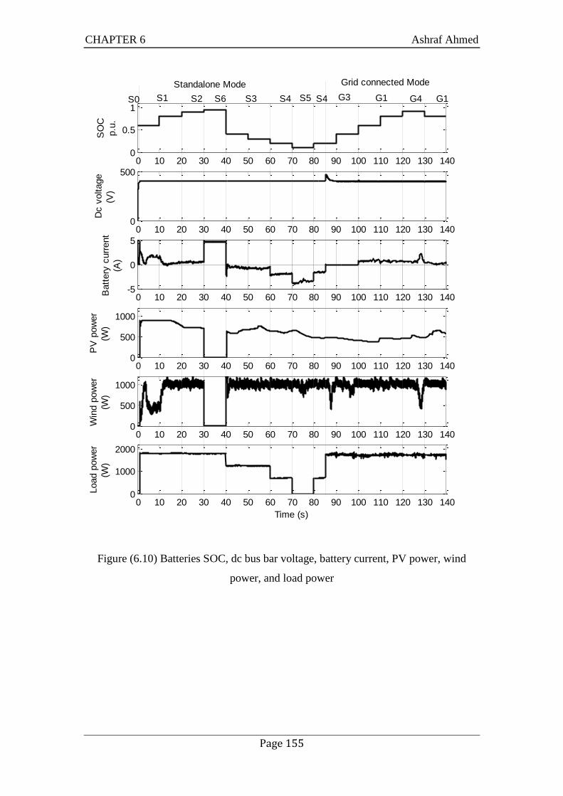
CHAPTER 6 Ashraf Ahmed
Page 155
Figure (6.10) Batteries SOC, dc bus bar voltage, battery current, PV power, wind
power, and load power
0 10 20 30 40 50 60 70 80 90 100 110 120 130 1400
0.5
1S
OC
p.u
.
0 10 20 30 40 50 60 70 80 90 100 110 120 130 1400
500
Dc v
oltage
(V)
0 10 20 30 40 50 60 70 80 90 100 110 120 130 140-5
0
5
Batt
ery
curr
ent
(A)
0 10 20 30 40 50 60 70 80 90 100 110 120 130 1400
500
1000
PV
pow
er
(W)
0 10 20 30 40 50 60 70 80 90 100 110 120 130 1400
500
1000
Win
d p
ow
er
(W)
0 10 20 30 40 50 60 70 80 90 100 110 120 130 1400
1000
2000
Time (s)
Load p
ow
er
(W)
S2 S6 S3 S4 G1
Grid connected ModeStandalone Mode
S0 S4S5 G1G3 G4S1
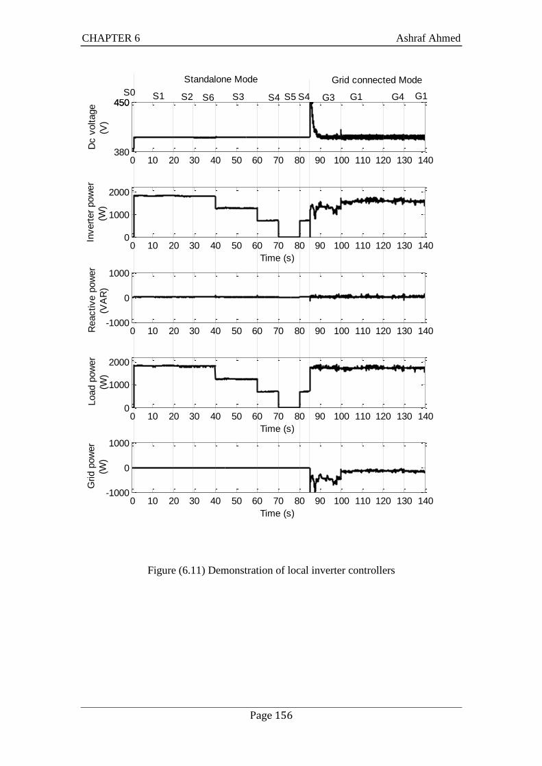
CHAPTER 6 Ashraf Ahmed
Page 156
Figure (6.11) Demonstration of local inverter controllers
0 10 20 30 40 50 60 70 80 90 100 110 120 130 140380
450450
Dc v
oltage
(V)
0 10 20 30 40 50 60 70 80 90 100 110 120 130 1400
1000
2000
Time (s)
Invert
er
pow
er
(W)
0 10 20 30 40 50 60 70 80 90 100 110 120 130 140-1000
0
1000
Reactive p
ow
er
(VA
R)
0 10 20 30 40 50 60 70 80 90 100 110 120 130 1400
1000
2000
Time (s)
Load p
ow
er
(W)
0 10 20 30 40 50 60 70 80 90 100 110 120 130 140-1000
0
1000
Time (s)
Grid p
ow
er
(W)
S2 S6 S4 G1 G1
Standalone Mode Grid connected Mode
S0G3 G4S1 S3 S4S5

CHAPTER 6 Ashraf Ahmed
Page 157
Figure (6.12) Ac side currents
0 10 20 30 40 50 60 70 80 90 100 110 120 130 140
-10
0
10
Invert
er
curr
ent
(A)
0 10 20 30 40 50 60 70 80 90 100 110 120 130 140
-10
0
10
Time (s)
Load c
urr
ent
(A)
0 10 20 30 40 50 60 70 80 90 100 110 120 130 140
-10
0
10
Grid c
urr
ent
(A)
Time (s)
S4 G3S5S6S2S1 G1G4G1
Grid connected ModeStandalone Mode
S3 S4S0

CHAPTER (7)
CONCLUSION
This chapter concludes the thesis, as summarized in the following sections:
7.1. WIND GENERATOR SIDE
An electrical control scheme to deal with MPPT at low and moderate wind speeds and
constant power soft stalling at excessive wind velocities has been proposed for small-
scale vertical axis wind turbines. The MPPT is based on a simple lookup table for the
characteristics of dc output voltage-current maximum power. The new constant
electrical power stalling is based on the concept of, and aims at, keeping the electrical
power and generator speed within limits. The method is the reverse of what is
normally used for MPPT control and completely avoids the need for explicitly finding
the target operating point, which changes with wind velocity. The system is modelled
and a PI controller designed. As the wind velocity increases beyond the rated value,
the system automatically enters the stall mode. A compensating 1st order lag is added
in the control loop to stabilize the system. It has been found that the time constant
needed increases, proportional to the turbine moment of inertia and the targeted
maximum wind velocity. With different turbine characteristics and application
scenarios, a customized design procedure was carried out to determine the PI control
gains and the 1st order lag time constant. To prevent reduction in MPPT efficiency,
the time constant was adapted online according to the current measured on the dc side
of the generator rectifier. The proposed control method has been tested by simulation
and laboratory experiment. Advantages of the proposed scheme include simplicity of
controller design, ease of implementation, avoidance for an anemometer or shaft
encoder, no need for aerodynamic control, and much reduced short-term over loading
requirement on the generator and power semi-conductor devices. The scheme has the
potential to reduce the cost and size of the wind turbine generator system.

CHAPTER 7 Ashraf Ahmed
Page 159
7.2. PV GENERATOR SIDE
Direct duty ratio control of the PV generator, which is based on hill climbing
algorithms, was described as a very advantageous method due to its simplicity and
ease of implementation. Therefore, it was chosen as the base of the control algorithm
for the PV generator side in this study. The design of the perturbation parameters for
this proposed method was always found favorable. It was reported that it would
guarantee better performance of the hill climbing MPPT controllers. It was also found
that, as a result, the MPPT efficiency would be increased, the fluctuation in power
reduced, and the output power quality of the system increased. Design guidelines for a
hill climbing algorithm perturbation parameters have also been proposed. The
effectiveness of the proposed guidelines was verified by simulation. The MPPT
controller combined with reduced power mode algorithm was developed, and it was
based on variable step size incremental conductance method. The proposed method
was easy to implement in simple microcontrollers, and it was fast compared to normal
fixed step incremental conductance, too. The reduced power mode was used to limit
the output power of the PV generator if the power generated was over the system
rating due to reduced ambient temperature values and high solar radiations. This mode
was also used if there was excess power generated in the system as it operated on
standalone mode. The algorithm was demonstrated by simulation and experimental
results.
7.3. INVERTER SIDE
Based on peak current control, a novel current controller was developed to control a
single-phase H-bridge inverter. The method was fast and easy to implement, and
adding selective harmonic elimination made the method corresponding to
international standards. This was demonstrated by simulation results. The method was
applied to grid-connected control, as it was used to inject active power keeping the
power factor and dc link voltage at specified values. To demonstrate the validity of
the method, simulation was applied on different active power levels, power factor
values and two quadrant operations. The simulation results were found adequate. The
standalone mode was required in this study so that the same method might be applied
to this operational mode. In this mode, the output ac voltage was required to be kept

CHAPTER 7 Ashraf Ahmed
Page 160
constant at different power levels. Simulation results were applied and they
demonstrated the control method. The issue of dc current injection has generally been
of growing concern due to the increasing usage of single-phase inverters as the
demand for small scale renewable power generation increases. One of the challenges
to eliminate the dc current injection is to accurately measure the small dc component
contained in the inverter output current, because the fundamental ac component is
very large. In this study, a method for eliminating the dc current injection of a single-
phase H-bridge inverter was proposed. The proposed method was based on designing
a passive filter to make the dc component more measurable in the filter output. A
simplified method for designing the compensating control was proposed for the
inverter PWM process. The method has been verified by both simulation and
experimental test. The simulation and test results demonstrated that the proposed
method improved the accuracy of measuring the very small dc current component.
This improvement helped with removing the dc component to meet the obligatory
local and international standards.
7.4. SUPERVISORY CONTROL
For the proposed small-scale hybrid PV-Wind generation systems, a supervisory
controller, which manages the modes of operation and the power flow in the power
system, was proposed. This controller was designed to operate in conjunction with the
newly developed local controllers. The system modes and states were designed to
provide system equilibrium conditions, and the characteristics of these modes were
held in specific constraints. Furthermore, the energy flow was balanced between the
system components. The number and the assemblies of those operating modes were
designed according to the system components and configurations. One of the
important controller rules was to guarantee smooth transition between the different
modes of operation. The proposed power management strategy depended on the SOC
of the battery storage and the utility grid availability. Furthermore, the supervisory
controller also set the local controllers for the different components on different
modes in order to ensure their optimum operation.
The system containing the entire power conditioning unit was modelled in Matlab/
Simulink with PLECS software. It included the supervisory controller and the local

CHAPTER 7 Ashraf Ahmed
Page 161
controllers for the different system components. The simulation ran took into account
the different modes and states of the system. The results demonstrated that the power
conditioning unit had a satisfactory performance and shifted between the different
operational modes and states smoothly.
7.5. THE CONTRIBUTIONS
The contributions in this thesis could be summarized as follows:
1. A constant power soft stalling controller is proposed for VAWT generator.
This is based on electrical control; therefore, it is simple, easy to design, and
easy to implement. As a result, it will reduce the cost and size and increase the
reliability of the VAWT generators.
2. Design guidelines for the perturbation parameters of the hill climbing
algorithm are provided in the PV generator side. These guidelines are expected
to increase the MPPT efficiency and improve the system performance.
3. A MPPT algorithm with reduced power mode based on variable step
incremental conductance is proposed and verified.
4. Dc current injection elimination method is proposed for the single phase H-
bridge inverter.
5. A new direct current control method for a single-phase H-bridge inverter is
derived. This method is based on peak current control and single harmonic
elimination.
6. Based on these proposed local controllers, a supervisory controller is also
proposed to manage the power between the different system components.
Furthermore, it supervises the local controller operations and system modes.
7.6. FUTURE WORK
The author believes that the power conditioning unit proposed in this study is the
future for such small-scale hybrid PV-Wind generation systems. The following points
would complete the work and make it available for the future market.
1. The proposed VAWT wind generator controller needs to be tested with
different wind turbines of different Cp-λ(TSR) curve shapes. It also has to be
applied in different power electronic configurations. Furthermore, this

CHAPTER 7 Ashraf Ahmed
Page 162
controller needs to be tested with a real wind turbine and implemented in a
microcontroller.
2. A microcontroller implementation is also required to the proposed PV
generator controller.
3. The peak current controller, which has been applied to the H-bridge inverter,
will experimentally be demonstrated.
4. The H-bride inverter and the proposed dc injection elimination circuit require
more testing.
5. Experimental set-up is required for the verification of the proposed system
with the power conditioning unit control.
6. A single layout integrating the converter power and control circuits will be
designed and tested in the future.
Bibliography Ashraf Ahmed
Page 163
References
[1] Organization Of The Petroleum Exporting Countries (OPEC). World oil outlook (2009).
[Online]: http://www.opec.org/opec_web/en/.
[2] Exxonmobil. Outlook for energy - A view to 2030. [Online]:
http://www.exxonmobil.com/.
[3] Energy Information Administration (EIA). International energy outlook (2009). [Online]:
www.eia.doe.gov/oiaf/ieo/index.html.
[4] E Martinot and J Sawin, "Renewables global status report 2009 update," Renewable Energy
World International Magazine, vol. 12, no. 4, 2009. [Online]:
http://www.ren21.net/globalstatusreport/g2009.asp.
[5] M Liserre, T Sauter, and J Hung, "Integrating renewable energy sources into the smart power
grid through industrial electronics," IEEE Industrial Electronics Magazine, vol. 4, no. 1, pp. 18-
37, 2010.
[6] British Wind Energy Association (BWEA). UK market report: Small wind systems. [Online]:
http://www.bwea.com/.
[7] Global Wind Energy Council (GWEC). Global Wind Report 2009. [Online]:
http://www.gwec.net/index.php?id=8.
[8] J Guerrero, F Blaabjerg, and T Zhelev, "Distributed Generation: Toward a New Energy
Paradigm," IEEE Industrial Electronics Magazine, vol. 4, no. 1, pp. 52 - 64 , 2010.
[9] International Energy Agency (IEA). Technology Roadmap: Solar Photovoltaic Energy.
[Online]: http://www.iea.org/.
[10] C Wang, L Wang, L Shi, and Y Ni, "A survey on wind power technologies in power systems,"
in IEEE-Power-Engineering-Society General Meeting, Tampa, USA, pp. 2268-2273, 2007.
[11] A. Ahmed, L. Ran, and J. R. Bumby, ―Sizing and Best Management of Stand Alone Hybrid PV-
Wind System using logistical model‖ IFAC conference on control methodologies and
technology for energy efficiency, Vilamoura, Portugal (CMTEE), 2010. [12] S Kim, J Jeon, C Cho, J Ahn, and S Kwon, "Dynamic modeling and control of a grid-connected
hybrid generation system with versatile power transfer," IEEE Transactions On Industrial
Electronics, vol. 55, no. 4, pp. 1677-1688, 2008.
[13] A Mirecki, X Roboam, and F Richardeau, "Architecture complexity and energy efficiency of
small wind turbines," IEEE Transactions On Industrial Electronics, vol. 54, no. 1, pp. 660-670,
2007.
[14] J Carrasco et al., "Power-electronic systems for the grid integration of renewable energy
sources: A survey," IEEE Transactions on Industrial Electronics, vol. 53, no. 4, pp. 1002–1016,
2008.
[15] K Chau, C Chan, and C Liu, "Overview of permanent-magnet brushless drives for electric and
hybrid electric vehicles," IEEE Transactions On Industrial Electronics, vol. 55, no. 6, pp. 2246–
2257, 2008.
[16] J Baroudi, V Dinavahi, and A Knight, "A review of power converter topologies for wind
generators," Renewable Energy, vol. 32, no. 14, pp. 2369–2385, 2007.
[17] D Hamill, "Power electronics: a field rich in nonlinear dynamics," in Specialists Workshop On
Nonlinear Dynamics Of Electronic Systems, Dublin, 1995, pp. 164-179.
[18] S Kjaer, J Pedersen, and F Blaabjerg, "A review of single-phase grid-connected inverters for
photovoltaic modules," IEEE Transactions On Industry Applications, vol. 41, no. 5, pp. 1292–
1306, 2005.
[19] R Gonzalez, J Lopez, P Sanchis, and L Marroyo, "Transformerless inverter for single-phase
photovoltaic systems," IEEE Transactions On Power Electronics, vol. 22, no. 2, pp. 693-697,
2007.
[20] T Kerekes, R Teodorescu, and E Aldabas, "A new high-efficiency single-phase transformerless
PV inverter topology," accepted for publication in IEEE Transactions on Industrial Electronics,
2010.
[21] G Spagnuolo et al., "Renewable energy operation and conversion schemes a summary of
discussions during the seminar on renewable energy systems," IEEE Industrial Electronics
Magazine, vol. 4, no. 1, pp. 38-51, 2010.
[22] M Armstrong, D Atkinson, C Johnson, and T Abeyasekera, "Auto-calibrating DC link current
sensing technique for transformerless grid connected h-bridge inverter systems," IEEE
Transactions on Power Electronics, vol. 21, no. 5, pp. 1385-1393, 2006.
[23] T Ackermann, Wind power in power systems.: John Wiley & Sons, 2005.

Bibliography Ashraf Ahmed
Page 164
[24] E Hau, Wind turbines : fundamentals, technologies, application, economics, 2006.
[25] T Burton, D Sharpe, N Jenkins, and E Bossanyi, Wind energy handbook.: John Wiley & Sons,
2001.
[26] M Prats et al., "A new fuzzy logic controller to improve the captured wind energy in a real 800
kW variable speed-variable pitch wind turbine," The 33rd Annual IEEE Power Electronics
Specialists Conference (PESC 02), vol. 1-4, pp. 101 - 105, 2002.
[27] B Boukhezzar, L Lupua, H Siguerdidjane, and M Hand, "Multivariable control strategy for
variable speed,variable pitch wind turbines," Renewable Energy, vol. 32, no. 8, pp. 1273-1287,
2007.
[28] E Muljadi and C Butterfield, "Pitch-controlled variable-speed wind turbine generation," in IEEE
Annual Meeting of The Industry-Applications-Society, Phoenix, USA, 2001, pp. 240 - 246.
[29] W Chen and Y Hsu, "Controller design for an induction generator driven by a variable-speed
wind turbine," IEEE Transactions On Energy Conversion, vol. 21, no. 3, pp. 625-635, 2006.
[30] W Chen and Y Hsu, "Unified voltage and pitch angle controller for wind-driven induction
generator system," IEEE Transactions On Aerospace and Electronic Systems, vol. 44, no. 3, pp.
913-926, 2008.
[31] Z Chen, J Guerrero, and F Blaabjerg, "A review of the state of the art of power electronics for
wind turbines," IEEE Transactions On Power Electronics, vol. 24, no. 8, pp. 1859 - 1875, 2009.
[32] S Hao, G Hunter, V Ramsden, and D Patters, "Control system design for a 20 kw wind turbine
generator with a boost converter and battery bank load," IEEE 32nd Annual Power Electronics
Specialists Conference (PESC), vol. 4, pp. 2203 - 2206, 2001.
[33] S Muyeen, R Takahashi, T Murata, and J Tamura, "A variable speed wind turbine control
strategy to meet wind farm grid code requirements," IEEE Transactions On Power Systems, vol.
25, no. 1, pp. 331 - 340, 2010.
[34] W Qiao, L Qu, and R Harley, "Control of IPM synchronous generator for maximum wind power
generation considering magnetic saturation," in 42nd Annual Meeting Of the IEEE -Industry-
Applications-Society, vol. 45, New Orleans, USA, 2009, pp. 1095-1105.
[35] M Ali, M Park, I Yu, T Murata, and J Tamura, "Improvement of wind-generator stability by
fuzzy-logic-controlled SMES," IEEE Transactions On Industry Applications, vol. 45, no. 3, pp.
1045-1051, 2009.
[36] N Nanayakkara, M Nakamura, and H Hatazaki, "Predictive control of wind turbines in small
power systems at high turbulent wind speeds," Control Engineering Practice, vol. 5, no. 8, pp.
1063-1069, 1997.
[37] M El Mokadem, C Nichita, B Dakyo, and W Koczara, "Maximum wind power control using
torque characteristic in a Wind diesel system with battery storage," The 6th International
Conference on Electrical Machines (ICEM), Cracow, Poland pp. 385-396, 2006.
[38] C Pournaras, A Soldatos, S Papathanassio, and A Kladas, "Robust controller for Variable Speed
Stall Regulated Wind Turbines," International Conference on Electrical Machines (ICEM'04),
Cracow, 2004.
[39] S Kim and E Kim, "PSCAD/EMTDC-based modeling and analysis of a gearless variable speed
wind turbine," IEEE Transactions On Energy Conversion, vol. 22, no. 2, pp. 421-430, 2007.
[40] M Malinowski, S Stynski, W Kolomyjski, and M Kazmierkowski, "Control of three-level PWM
converter applied to variable-speed-type turbines," IEEE International Conference on Industrial
Technology, Bombay, India, vol. 56, pp. 69-77, 2009.
[41] K Yuen et al., "Matching a permanent magnet synchronous generator to a fixed pitch vertical
axis turbine for marine current energy conversion," IEEE Journal Of Oceanic Engineering, vol.
34, no. 1, pp. 24-31, 2009.
[42] M Simoes, B Bose, and R Spiegel, "Design and performance evaluation of a fuzzy-logic-based
variable-speed wind generation system," in 32nd Annual Meeting Of The IEEE Industry-
Applications-Society, New Orleans, USA, vol. 33, pp. 956 - 965, 1997.
[43] B Bose and M Simões, "Fuzzy logic based intelligent control of a variable speed cage machine
wind generation system," IEEE Transactions on Power Electronics, vol. 33, no. 4, pp. 956-965,
1997.
[44] A Abo-Khalil, D Lee, and J Seok, "Variable speed wind power generation system based on
fuzzy logic control for maximum output power tracking," IEEE 35th Annual Power Electronics
Specialists Conference, Aachen, Germany, pp. 2039-2042, 2004.
[45] W Qiao, W Zhou, J Aller, and R Harley, "Wind speed estimation based sensorless output
maximization control for a wind turbine driving a DFIG," IEEE Transactions On Power
Electronics, vol. 23, no. 3, pp. 1156-1169, 2008.

Bibliography Ashraf Ahmed
Page 165
[46] H Li, K Shi, and P McLaren, "Neural-network-based sensorless maximum wind energy capture
with compensated power coefficient," IEEE Transactions On Industry Applications, vol. 41, no.
6, pp. 1548-1556, 2005.
[47] H Li, D Zhang, and S Foo, "A stochastic digital implementation of a neural network controller
for small wind turbine systems," IEEE Transactions On Power Electronics, vol. 21, no. 5, pp.
1502-1507, 2006.
[48] M Chinchilla, S Arnaltes, and J Burgos, "Control of permanent-magnet generators applied to
variable-speed wind-energy systems connected to the grid," IEEE Transactions On Energy
Conversion, vol. 21, no. 1, pp. 130-135, 2006.
[49] A Ahmed, Li Ran, and J Bumby, "Simulation and control of a hybrid PV-wind system," IET 4th
Conference on Power Electronics, Machines and Drives, pp. 421- 425, 2008.
[50] M Parker, P Tavner, L Ran, and A Wilson, "A low cost power-tracking controller for a small
vertical axis wind turbine," The 40th International Universities Power Engineering Conference,
Cork, Ireland, 2005.
[51] A Knight and G Peters, "Simple wind energy controller for an expanded operating range," IEEE
Transactions On Energy Conversion, vol. 20, no. 2, pp. 459-466, 2005.
[52] S Dehghan, M Mohamadian, and A Yazdian, "A new variable-speed wind energy conversion
system using permanent-magnet synchronous generator and Z-source inverter," IEEE
Transactions On Energy Conversion, vol. 24, no. 3, pp. 714-724, 2009.
[53] T Senjyu et al., "Wind velocity and rotor position sensorless maximum power point tracking
control for wind generation system," Renewable Energy, vol. 31, no. 11, pp. 1764-1775, 2006.
[54] S Morimoto, H Nakayama, M Sanada, and Y Takeda, "Sensorless output maximization control
for variable-speed wind generation system using IPMSG," 38th IEEE Annual Meeting of the
Industry-Applications-Society, Salt Lake, USA, vol. 41, pp. 60-67, 2005.
[55] T Senjyu et al., "Sensor-less maximum power point tracking control for wind generation system
with squirrel cage induction generator," Renewable Energy, vol. 34, no. 4, pp. 994–999, 2009.
[56] B Shen, B Mwinyiwiwa, Y Zhang, and B Ooi, "Sensorless maximum power point tracking of
wind by DFIG using rotor position phase lock loop (PLL)," IEEE Transactions On Power
Electronics, vol. 24, no. 4, pp. 942-951, 2009.
[57] C Pan and Y Juan, "A novel sensorless MPPT controller for a high-efficiency microscale wind
power generation system," IEEE Transactions On Energy Conversion, vol. 25, no. 1, pp. 207-
216, 2010.
[58] N Mutoh and A Nagasawa, "A maximum power point tracking control method suitable for
compact wind power generators," IEEE Power Electronics Specialists Conference, vol. 1-7,
Cheju Isl, South Korea, pp. 1740-1746, 2006.
[59] A Raju, K Chatterjee, and B Fernandes, "A simple maximum power point tracker for grid
connected variable speed wind energy conversion system with reduced switch count power
converters," IEEE 34TH Annual Power Electronics Specialists Conference, vol. 2, Acapulco,
Mexico, pp. 748-753, 2003.
[60] Q Wang and L Chang, "An intelligent maximum power extraction algorithm for inverter-based
variable speed wind turbine systems," IEEE Transactions On Power Electronics, vol. 19, no. 5,
pp. 1242-1249, 2004.
[61] T Tanaka, T Toumiya, and T Suzuki, "Output control by Hill-climbing method For a small scale
wind power generating system," Renewable Energy, vol. 12, no. 4, pp. 387-400, 1997.
[62] R Datta and V Ranganathan, "A method of tracking the peak power points for a variable speed
wind energy conversion system," IEEE Transactions On Energy Conversion, vol. 18, no. 1, pp.
163-167, 2003.
[63] C Liu, K Chau, and X Zhang, "An efficient wind–photovoltaic hybrid generation system using
doubly excited permanent-magnet brushless machine," IEEE Transactions On Industrial
Electronics, vol. 57, no. 3, pp. 831 - 839, 2010.
[64] E Koutroulis and K Kalaitzakis, "Design of a maximum power tracking system for wind-
energy-conversion applications," IEEE Transactions On Industrial Electronics, vol. 53, no. 2,
pp. 486-494, 2006.
[65] S Barakati, M Kazerani, and J Aplevich, "Maximum power tracking control for a wind turbine
system including a matrix converter," IEEE Transactions On Energy Conversion, vol. 24, no. 3,
pp. 705-715, 2009.
[66] R Hilloowala and A Sharaf, "A rule-based fuzzy logic controller for a PWM inverter in a stand
alone wind energy conversion scheme," IEEE Transactions On Industry Applications, vol. 32,
no. 1, pp. 57-65, 1996.

Bibliography Ashraf Ahmed
Page 166
[67] F Bianchi, R Mantz, and C Christiansen, "Power regulation in pitch-controlled variable speed
WECS above rated wind speed," Renewable Energy, vol. 29, no. 11, pp. 1911-1922, 2004.
[68] H Camblong, "Digital robust control of a variable speed pitch regulated wind turbine for above
rated wind speeds," Control Engineering Practice, vol. 16, no. 8, pp. 946–958, 2008.
[69] L Pak and V Dinavahi, "Real-time simulation of a wind energy system based on the doubly-fed
induction generator," IEEE Transactions On Power Systems, vol. 24, no. 3, pp. 1301-1309,
2009.
[70] T Barlas and G van-Kuik, "State of the art and prospectives of smart rotor control for wind
turbines," Journal of Physics: Conference Series, vol. 75, no. 1, 2007.
[71] E Muljadi, K Pierce, and P Migliore, "Control strategy for variable-speed, stall-regulated wind
turbines," American Control Conference, vol. 1-6, Philadelphia, USA, 1998, pp. 1710-1714.
[72] A Miller, E Muljadi, and D Zinger, "A variable speed wind turbine power control," IEEE
Transactions On Energy Conversion, vol. 12, no. 2, pp. 181 - 186, 1997.
[73] A Haniotis, K Soutis, A Kladas, and J Tegopoulos, "Grid connected variable speed wind turbine
modeling, dynamic performance and control," IEEE PES Power Systems and Exposition
Conference, vol. 1- 3, New York, USA, pp. 759 - 764, 2004.
[74] E Muljadi, K Pierce, and P Migliore, "Soft-stall control for variable-speed stall-regulated wind
turbines," Journal Of Wind Engineering And Industrial Aerodynamics, vol. 85, no. 3, pp. 277-
291, 2000.
[75] J Bumby, N Stannard, J Dominy, and N McLeod, "A permanent magnet generator for small
scale wind and water turbines," in International Conferece On Electrical Machines, vol. 1- 4,
Vilamoura, Portugal, 2008, pp. 196-201.
[76] E Elshenawy and A Bahjet, ―Development and implementation of maximum power point
tracking controller for PV system using neural networks,‖ Cairo university, Giza, Egypt, PhD
Thesis 2002.
[77] A Ahmed, O Mahgoub, and K Elmetwally, ―Using neural networks photovoltaic system
modeling in maximum power point tracking,‖ Cairo university, Giza, Egypt, M.Sc. Thesis 2005.
[78] A Özcan, y Mehmet, and E Feriha, ―Application of genetic algorithms on a photovoltaic panel
(PV)-pump motor matching to natural tracking of PV maximum power points,‖ in nternational
XII. Turkish Symposium on Artificial Intelligence and Neural Networks (TAINN), vol. 1,
Canakkale Turkiye, 2003.
[79] D Hohm and M Ropp, ―Comparative study of maximum power point tracking algorithms using
an experimental, programmable, maximum power point tracking test bed,‖ IEEE 28th
Photovoltaic Specialists Conference, Anchorage, USA, pp. 1699-1702, 2000.
[80] M Saied, ―Improved matching of photovoltaic solar arrays supplying DC motors through
controlled motor saturation,‖ 11th
International Conference On Microelectronics (ICM99),
Kuwait, Kuwait, pp. 275-279, 1999.
[81] M Saied, ―The available matching of solar arrays to dc motors having both constant and series-
excited field components,‖ IEEE Transaction On Energy Conversion, vol. 17, no. 3, pp. 301-
305, 2002.
[82] M Saied, ―The advantages of using saturable DC series motors fed from solar photovoltaic
arrays,‖ Electric Machines And Power Systems, vol. 28, no. 8, pp. 677-687, 2000.
[83] H Ibrahim, F Houssiny, H El-Din, and M El-Shibini, ―Microcomputer controlled buck regulator
for maximum power point tracker for DC pumping system operates from photovoltaic system,‖
IEEE International Conference Proceedings For Fuzzy Systems, vol. 1, Seoul, South Korea, pp.
406-411, 1999.
[84] W Swiegers and J Enslin, ―An integrated maximum power point tracker for photovoltaic
panels,‖ IEEE International Symposium On Industrial Electronics, vol. 1 and 2, pp. 40-44, 1998.
[85] M Masoum, ―Optimal power point tracking of photovoltaic system under all operating
conditions,‖ , Houston, Texas, 1998.
[86] S Alghwainem, ―Matching of a dc motor to a photovoltaic generator using a step-up converter
with a current-locked loop,‖ IEEE Transactions On Energy Conversion, vol. 9, no. 1, pp. 192-
198, 1994.
[87] M Masoum, A Mohammad, S Dehbonei, and A Hooman, ―Design construction and testing of a
voltage-based maximum power point tracker (VMPPT) for small satellite power supply,‖ The
13th
Annual AIAA/USU Conference on Small Satellites, pp. 1-12, 1999.
[88] S Togashi, T Noguchi, and R Nakamoto, ―Short-Current pulse based maximum-power-point
operation of photovoltaic generation system,‖ Conference in proceeding of IEEJ/IAS, vol. 3, pp.
221–224, 1999.

Bibliography Ashraf Ahmed
Page 167
[89] T Noguchi, S Togashi, and R Nakamoto, ―Short-current pulse-based maximum-power-point
tracking method for multiple photovoltaic-and-converter module system,‖ IEEE Transactions
On Inustrial Electronics, vol. 49, no. 1, pp. 217-223, 2002.
[90] C Hua, J Lin, and C Shen, ―Implementation of a DSP_ controlled photovoltaic system with peak
power tracking,‖ IEEE Transactions On Inustrial Electronics, vol. 45, no. 1, pp. 99-107, 1998.
[91] O Wasynczuk, ―Dynamic behavior of a class of photovoltaic power systems,‖ IEEE
Transactions On Power Application Systems, vol. 102, no. 9, pp. 3031–3037, 1983.
[92] N Kasa, T Iida, and L Chen, ―Fyack inverter controlled by sensorless current MPPT for
photovoltaic power system,‖ IEEE Transactions On Industrial Electronics, vol. 52, no. 4, pp.
1145–1152, 2005.
[93] Y Kim, H Jo, and D Kim, ―A new peak power tracker for cost-effective photovoltaic power
systems,‖ The 31st Intersociety Energy Conversion Engineering Conference (IECEC 96), pp.
1673–1678, 1996.
[94] Y Chen and K Smedley, ―A cost-effective single-stage inverter with maximum power point
tracking,‖ IEEE Transaction On Power Electronics, vol. 19, no. 5, pp. 1289-1294, 2004.
[95] E, Kalaitzakis, K Koutroulis and N Voulgaris, ―Development of a microcontroller-based,
photovoltaic maximum power point tracking control system,‖ IEEE Transactions On Power
Electronics, vol. 16, no. 1, pp. 46-54, 2001.
[96] D Snyman and J Enslin, ―Simplified maximum power point controller for PV installations,‖ The
IEEE 23rd
Photovoltaic Specialists Conference, Louisville, USA, pp. 1240-1245, 1993.
[97] H Koizumi and K Kurokawa, ―A novel microcontroller for grid-connected photovoltaic
systems,‖ IEEE Transactions On Industrial Electronics, vol. 53, no. 6, pp. 1889-1897, 2006.
[98] K Hussein, I Muta, T Hoshino, and M Osakada, ―Maximum photovoltaic power tracking: An
algorithm for rapidly changing atmospheric conditions,‖ IEE Proceedings-Generation
Transmission And Distrbution, vol. 142, no. 1, pp. 59-64, 1995.
[99] W Wu et al., ―DSP-based multiple peak power tracking for expandable power system,‖ in IEEE
18th
Annual Applied Power Electronics Conference and Exposition, vol. 1 and 2, Miami, USA,
pp. 525- 530, 2003.
[100] Y Kuo, T Liang, and J Chen, ―Novel maximum-power-point-tracking controller for photovoltaic
energy conversion system,‖ IEEE Transactions On Industrial Electronics, vol. 48, no. 3, pp.
594-601, 2001.
[101] A Nafeh, F Fahmy, O Mahgoub, and E Abouelzahab, ―Developed algorithm of maximum power
tracking for stand alone photovoltaic system,‖ Energy Sources, vol. 20, no. 1, pp. 45-53, 1998.
[102] A Bahgat, N Helwa, G Ahmad, and E El Shenawy, ―Maximum power point traking controller
for PV systems using neural networks,‖ Renewable Energy, vol. 30, no. 8, pp. 1257-1268, 2005.
[103] I Cha et al., ―MPPT for temperature compensation of photovoltaic system with neural
networks,‖ in IEEE 26th
Photovoltaic Specialists Conference, Anaheim, USA, pp. 1321-1324,
1997.
[104] A Ahmed, K El-Metwally, and O Mahgoub, ―A photovoltaic intelligent power conditioning unit
for MPPT using neural networks,‖ in 5th
International Engineering Conference, Sharm El-Shikh,
Egypt, vol. 1, 2006.
[105] G Yu, M Jung, J Song, I Cha, and I Hwang, ―Maximum power point tracking with temperature
compensation of photovoltaic For air conditioning system with fuzzy controller,‖ in IEEE 25th
Photovoltaic Specialists Conference, Washington, USA, pp. 1429-1432, 1996.
[106] W Tsai-Fu, C Chien-Hsuan, and C Yu-Hai, ―A fuzzy-logic-controlled single-stage converter for
PV-powered lighting system applications,‖ IEEE Transactions On Industrial Electronics, vol.
47, no. 2, pp. 287-296, 2000.
[107] V Salas, E Olías, A Barrado, and J Pleite, ―Novel algorithm applied to maximum power point
trackers (MPPT) measuring only one photovoltaic variable,‖ in 1ST
SWH International
Conference: Solar-Wind-Hydrogen/Fuel Cells-(Renewable Energies), Segovia, España., 2003.
[108] V Salas, E Olias, A Lazaro, and A Barrado, ―Evaluation of a new maximum power point tracker
(MPPT) applied to the photovoltaic stand-alone systems,‖ Solar Energy Materials And Solar
Cells, vol. 87, no. 1-4, pp. 807-815, 2005.
[109] G Grandi, D Casadei, and C Rossi, ―Direct coupling of power active filters with photovoltaic
generation systems with improved MPPT capability,‖ in IEEE Bologna Power Tech Conference
Proceedings, vol. 2, p. 6, 2003.
[110] K Irisawa, T Saito, I Takano, and Y Sawada, ―Maximum power point tracking control of
photovoltaic generation system under non-uniform insolation by means of monitoring cells,‖ in
IEEE 28th
Photovoltaic Specialists Conference, Anchorage, USA, pp. 1707-1710, 2000.

Bibliography Ashraf Ahmed
Page 168
[111] M Ned, M Tore, and P William, Power electronics: converters, applications, and design.: John
Wiley & Sons, 2003.
[112] [147]A Hava, R Kerkman, and T Lipo, ―Carrier-based PWM-VSI overmodulation strategies:
Analysis, comparison, and design,‖ IEEE Transactions On Power Electronics, vol. 13, no. 4, pp.
674-689, 1998.
[113] A Yazdian-Varjani, S Perera, and J Chicharo, ―A centroid-based PWM switching technique for
full-bridge inverter applications,‖ IEEE Transactions On Power Electronics, vol. 13, no. 1, pp.
115-124, 1998.
[114] R Lai and K Ngo, ―A PWM method for reduction of switching loss in a full-bridge inverter,‖
IEEE Transactions On Power Electronics, vol. 10, no. 3, pp. 326–332, 1995.
[115] T Ai, J Chen, and T Liang, ―A random switching method for HPWM full-bridge inverter,‖ IEEE
Transactions On Industrial Electronics, vol. 49, no. 3, pp. 595-597, 2002.
[116] C Cecati, A Dell, M Liserre, and V Monopoli, ―Design of hbridge multilevel active rectifier for
traction systems,‖ IEEE Transactions On Industry Applications, vol. 39, no. 5, pp. 1541-1550,
2003.
[117] Fukuda S and Yoda T, ―A novel current-tracking method for active filters based on a sinusoidal
internal model,‖ IEEE Transactions On Industry Applications , vol. 37, no. 3, pp. 888-895,
2001.
[118] R Teodorescu, F Blaabjerg, and U Liserre, ―A new control structure for grid-connected LCL PV
inverters with zero steady-state error and selective harmonic compensation,‖ in 19th
Annual
IEEE Applied Power Electronics Conference (APEC), vol. 1, Aachen, Germany, pp. 580 – 586,
2004.
[119] B Bose, ―An adaptive hysteresis–band current control technique of a voltage-fed PWM inverter
for machine drive system,‖ IEEE Transactions On Industerial Electronics, vol. 37, no. 5, pp.
402–408, 1990.
[120] B Fernandes, S Pillai, and V Subbarao, ―Performance of an adaptive hysteresis band current
controlled induction motor drive,‖ in International Conference On Industrial Electronics Control
Instrumentation And Automation ( IECON 92 ), vol. 1, San Diego, USA, pp. 447 – 452, 1992.
[121] C Pan, Y Huang, and T Jong, ―A constantly sampled current controller with switch status
dependent inner bound,‖ IEEE Transactions On Industrial Electronics, vol. 50, no. 3, pp. 528-
535, 2003.
[122] G Bode and D Holmes, ―Implementation of three level hysteresis current control for a single
phase voltage source inverter,‖ in IEEE 31st Annual Power Electronics Specialists Conferance,
vol. 1-3, Galway, Ireland, pp. 33-38, 2000.
[123] M Bech, F Blaabjerg, and J Pedersen, ―Random modulation techniques with fixed switching
frequency for three-phase power converters,‖ IEEE Transactions On Power Electronics, vol. 15,
no. 4, pp. 753-761, 2000.
[124] K Low, ―A digital control technique for a single-phase PWM inverter,‖ IEEE Transactions On
Industrial Electronics, vol. 45, no. 4, pp. 672-674, 1998.
[125] K Low, ―A DSP-based single-phase AC power source,‖ IEEE Transactions On Industrial
Electronics, vol. 46, no. 5, pp. 936-941, 1999.
[126] H Abu-Rub, J Guzin´ski, Z Krzeminski, and H Toliyat, ―Predictive current control of voltage-
source inverters,‖ IEEE Transactions On Industrial Electronics, vol. 51, no. 3, pp. 585-593,
2004.
[127] L Kay-Soon and C Runzi, ―Model Predictive Control of Parallel-Connected Inverters for
Uninterruptible Power Supplies,‖ IEEE Transactions On Industrial Electronics, vol. 55, no. 8,
pp. 2884-2893, 2008.
[128] H Kojabadi, B Yu, I Gadoura, and M Ghribi, ―A novel DSP-based current-controlled PWM
strategy for single phase grid connected inverters,‖ IEEE Transactions On Power Electronics,
vol. 21, no. 4, pp. 985-993, 2006.
[129] C Meza, J Negroni, D Biel, and F Guinjoan, "Energy-balance modeling and discrete control for
single-phase grid-connected PV central inverters," IEEE Transactions On Industrial Electronics,
vol. 55, no. 7, pp. 2734-2743, 2008.
[130] M Datta, T Senjyu, A Yona, T Funabashi, and C Kim, "A coordinated control method for
leveling PV output power fluctuations of PV–Diesel hybrid systems connected to isolated power
utility," IEEE Transaction On Energy Conversion, vol. 24, no. 1, pp. 153-162, 2009.
[131] L Hassaine, E Olias, and J Quintero, "Digital power factor control and reactive power regulation
for grid-connected photovoltaic inverter," Renewable Energy, vol. 34, no. 1, pp. 315–321, 2009.
Bibliography Ashraf Ahmed
Page 169
[132] J Liu, J Yang, and Z Wang, "A new approach for single-phase harmonic current detecting and
its application in a hybrid active power filter," in The 25th Annual Conference of the IEEE
Industrial Electronics Society (IECON '99), vol. 2, San Jose, USA, pp. 849 - 854, 1999.
[133] V Khadkikar, A Chandra, and B Singh, "Generalised single-phase p-q theory for active power
filtering: simulation and DSP-based experimental investigation," IET Power Electronics, vol. 2,
no. 1, pp. 67 - 78, 2009.
[134] J Correa, F Farret, and M Simoes, "Application of a modified single-phase P-Q theory in the
control of shunt and series active filters in a 400 hz microgrid," in 6th Annual IEEE Power
Electronic Specialists Conference, vol. 1-3, Recife, Brazil, pp. 2585 - 2591, 2005.
[135] T Wu, H Nien, C Shen, and T Chen, "A single-phase inverter system for PV power injection and
active power filtering with nonlinear inductor consideration," IEEE Transactions On Industry
Applications, vol. 41, no. 4, pp. 1075-1083, 2005.
[136] M Ryan, W Brumsickle, and R Lorenz, "Control topology options for single-phase UPS
inverters," IEEE Transactions On Industry Applications, vol. 33, no. 2, pp. 493-500, 1997.
[137] W Stefanutti and P Mattavelli, "Fully digital hysteresis modulation with switching-time
prediction," IEEE Transactions On Industry Applications, vol. 42, no. 3, pp. 763-769, 2006.
[138] A Kawamura and R Hoft, "Instantaneous feedback controlled PWM inverter with adaptive
hysteresis," IEEE Transactions On Industry Applications, vol. 20, no. 4, pp. 769–775, 1984.
[139] O Kukrer, H Kmurcugil, and N BaYlndlr, "Control strategy for single-phase UPS inverters,"
IEE Proceedings-Electric Power Applications, vol. 150, no. 6, pp. 743-746, 2003.
[140] M Ryan and R Lorenz, "A high-performance sine wave inverter controller with capacitor
current feedback and ―Back-EMF‖ decoupling," in 26th Annual Power Electronics Specialists
Conference (PESC 95), vol. 1-2, Atlanta, USA, pp. 507–513, 1995.
[141] T Kawabata, Y Shikano, and S Higashino, "Chargerless UPS using multi-functional BIMOS
inverter—sinusoidal voltage waveform inverter with current minor loop," in IEEE IAS Annual
Meeting Conferance, Denver, USA, pp. 513–520, 1986.
[142] V Salas, M Alonso, and F Chenlo, "Overview of the legislation of DC injection in the network
for low voltage small grid-connected PV systems in Spain and other countries," Renewable and
Sustainable Energy Reviews, pp. 575-583, 2008.
[143] R González, E Gubía, J López, and L Marroyo, ―Transformerless single-phase multilevel-based
photovoltaic inverter,‖ IEEE Transactions On Industrial Electronics, vol. 55, no. 7, pp. 2694-
2702, 2008.
[144] H Haeberlin, "Evolution of inverters for grid connected PV-Systems from 1989 to 2000," in
Proceedings Of The 17th European Photovoltaic Solar Energy Conference, Munich, Germany,
pp. 426–430, 2001.
[145] V Salas, M Alonso, E Olias, F Chenlo, and A Barrado, "DC current injection into the network
from PV inverters of less than 5 kW for low voltage small grid-connected PV systems ," Solar
Energy Materials and Solar Cells, vol. 91, no. 9, pp. 801–806, 2007.
[146] V Salas, E Olias, M Alonso, F Chen, and A Barrado, "DC current injection into the network
from PV grid inverters," in IEEE 4th World Conference On Photovoltaic Energy Conversion,
vol. 2, Waikoloa, USA, pp. 2371 – 2374, 2006.
[147] M khan, "Supervisory hybrid control of a wind energy conversion and battery storage system,"
Graduate Department Of Electrical And Computer Engineering, University of Toronto, PHD
thesis 2008.
[148] M Lemmon, K He, and I Markovesky, "Supervisory hybrid systems," IEEE Control Systems
Magazine, vol. 19, no. 4, pp. 42-55, 1999.
[149] P Antsaklis and A Nerode, "Guest editorial hybrid control systems an introductory discussion to
the special issue," IEEE Transactions On Automatic Control, vol. 43, no. 4, pp. 457-460, 1998.
[150] F Valenciaga and P Puleston, "Supervisor control for a stand-alone hybrid generation system
using wind and photovoltaic energy," IEEE Transactions On Energy Conversion, vol. 20, no. 2,
pp. 398-405, 2005.
[151] M Khan and M Iravani, "Hybrid control of a grid-interactive wind energy conversion system,"
IEEE Transactions On Energy Conversion, vol. 23, no. 3, pp. 895-902, 2008.
[152] C Wang and M Nehrir, "Power management of a stand-alone wind/photovoltaic/fuel cell energy
system," IEEE Transactions On Energy Conversion, vol. 23, no. 3, pp. 957-967, 2008.
[153] D Ipsakisa, S Voutetakisa, P Seferlis, F Stergiopoulosa, and C Elmasides, "Power management
strategies for a stand-alone power system using renewable energy sources and hydrogen
storage," Internation Journal Of Hyderogen energy, vol. 34, no. 16, pp. 7081-7095, 2009.

Bibliography Ashraf Ahmed
Page 170
[154] T Gebre, T Undeland, O Ulleberg, and P Vie, "Optimal load sharing strategy in a hybrid power
system based on PV/Fuel Cell/ Battery/Supercapacitor," in International Conference On Clean
Electrical Power, Capri, Itali, pp. 141-146, 2009.
[155] W Irena et al., "A power-quality management algorithm for low-voltage grids with distributed
resources," IEEE Transactions On Power Delivery, vol. 23, no. 2, pp. 1055-1062, 2008.
[156] S Teleke, M Baran, A Huang, S Bhattachar, and L Anderson, "Control strategies for battery
energy storage for wind farm dispatching," IEEE Transactions On Energy Conversion, vol. 24,
no. 3, pp. 725-732, 2009.
[157] S Daniel and N Gounden, "A novel hybrid isolated generating system based on PV fed inverter-
assisted wind-driven induction generators," IEEE Transactions On Energy Conversion, vol. 19,
no. 2, pp. 416-422, 2004.
[158] L Krichen, A Ouali, and G Boukettaya, "Fuzzy logic supervisor for power control of an isolated
hybrid energy production unit," International Journal of Electrical and Power Engineering, vol.
1, no. 3, pp. 279-285, 2007.
[159] E El Mokadem, V Courtecuisse, and C Saudemont, "Fuzzy logic supervisor-based primary
frequency control experiments of a variable-speed wind generator," IEEE Transactions on
Power Systems, vol. 24, no. 1, 2009.
[160] G Cimuca, C Saudemont, B Robyns, and M Radulescu, "Control and performance evaluation of
a flywheel energy-storage system associated to a variable-speed wind generator," IEEE
Transactions On Industrial Electronics, vol. 53, no. 4, pp. 1074-1085, 2006.
[161] C Abbey and G Joos, "Supercapacitor energy storage for wind energy applications," in 40th
Annual Meeting Of The IEEE-Industry-Applications-Society, vol. 43, Hong Kong, China, pp.
769-776, 2007.
[162] M Datta, T Senjyu, A Yona, and T Funabash, "A fuzzy control based coordinated method for
isolated power utility connected clustered photovoltaic systems to provide frequency control," in
IEEE 15th International Conference On Intelligent System Applications To Power Systems,
Curitiba, Brazil, pp. 1-6, 2009.
[163] L Krichen, B Francois, and A Ouali, "A fuzzy logic supervisor for active and reactive power
control of a fixed speed wind energy conversion system," Electric Power Systems Research, vol.
78, no. 3, pp. 418–424, 2008.
[164] R Welch and G Venayagamoorthy, "Optimal control of a photovoltaic solar energy system with
adaptive critics," in IEEE International Joint Conference On Neural Networks, vol. 1-6,
Orlando, USA, pp. 985-990, 2007.
[165] J Hui and A Bakhshai, "A new adaptive control algorithm for maximum power point tracking
for wind energy conversion systems," in IEEE Power Electronics Specialists Conferance (PESC
08), vol. 1-10, Rhodes, Greece, 2008, pp. 4003–4007.
[166] F Valenciaga and P Puleston, "High-order sliding control for wind energy conversion system
based on a permanent magnet synchronous generator," IEEE Transactions On Energy
Conversion, vol. 23, no. 3, pp. 860–867, 2008.
[167] B Beltran, T Ali, and M Benbouzid, "Sliding mode power control of variable-speed wind energy
conversion systems," IEEE Transactions On Energy Conversion, vol. 23, no. 2, pp. 551–558,
2008.
[168] J Mauricio, A Leon, A Gomez-Exposito, and J Solsona, "An adaptive nonlinear controller for
DFIM-based wind energy conversion systems," IEEE Transactions On Energy Conversion, vol.
23, no. 4, pp. 1025–1035, 2008.
[169] R Cardenas and R Pena, "Sensorless vector control of induction machines for variable-speed
wind energy applications," IEEE Transactions On Energy Conversion, vol. 19, no. 1, pp. 196–
205, 2004.
[170] B Kirke, "Evaluation of self-starting vertical axis wind turbines for stand-alone applications,"
Australia, 1998.
[171] J Bumby and R Martin, "An axial flux air-cored generator: The Savonius Generator," Durham,
Uk, 2005.
[172] dSPACE,(2006, October). [Online]:
http://www.dspace.ltd.uk/ww/en/ltd/home/products/hw/singbord/ppcconbo.cfm.
[173] T Esram and P Chapman, ―Comparison of photovoltaic array maximum power point tracking
techniques,‖ IEEE Transactions On Energy Conversion, vol. 22, no. 2, pp. 439-449, 2007.
[174] J Duffie and W Beckman, Solar engineering of thermal processes.: John Wiley & Sons, 2006.
[175] W Johnston, Solar voltaic cells. New York, , USA: Marcel Dekker, Inc, 1980.
[176] A Ahmed, O Mahgoub, and K El-Metwally, ―Neural networks based photovoltaic model,‖ in
Tenth Middle East Power Systems Conference , 2005.

Bibliography Ashraf Ahmed
Page 171
[177] T Townsend, ―A simplified method for estimating the long term performance of direct-
coupled,‖ Mechanical Engineering,Universty of Wisconsin-Madison, M.S. Thesis 1989.
[178] W Levine, The control handbook.: CRC Press in cooperation with IEEE Press, 1996.
[179] F Giraud and Z Salameh, ―Steady-state performance of a grid-connected rooftop hybrid wind–
photovoltaic power system with battery storage,‖ IEEE Transactions On Energy Conversion,
vol. 16, no. 1, pp. 1-7, 2001.
[180] T Suntio, ―Analysis and modeling of peak-current-mode-controlled buck converter in DICM,‖
IEEE Transactions On Industrial Electronics, vol. 48, no. 1, pp. 127-135, 2001.
[181] R Sheehan. (2007) [Online]:
http://powerelectronics.com/power_management/pwm_controllers/model-current-mode-control-
0507/.
[182] F Tan and R Middlebrook, "A unified model for current-programmed converters," IEEE
Transactions On Power Electronics, vol. 10, no. 4, pp. 397–408, 1995.
[183] G Andersen and F Blaabjerg, "Current programmed control of a single-phase two-switch buck–
boost power factor correction circuit," IEEE Transactions On Industrial Electronics, vol. 53, no.
1, pp. 263-271, 2006.
[184] C Deisch, "Simple switching control method changes power converter into a current source," in
IEEE Power Electronics Specialists Conference, Syracuse, USA, 1978, pp. 300–304.
[185] M Aimé, G Gateau, and T Meynard, "Implementation of a peak-current-control algorithm
within a field-programmable gate array," IEEE Transactions On Industrial Electronics, vol. 54,
no. 1, pp. 406-418, 2007.
[186] R Middlebrook, "Modeling current-programmed buck and boost regulators," IEEE Transactions
On Power Electronics, vol. 4, no. 1, pp. 36-52, 1989.
[187] S Mazumder, A Nayfeh, and D Boroyevich, "Theoretical and experimental investigation of the
fast- and slow-scale instabilities of a DC-DC converter," IEEE Transactions On Power
Electronics, vol. 16, no. 2, pp. 201-216, 2001.
[188] I Zafrany and S Ben-yaakov, "A chaos model of subharmonic oscillations in current mode
PWM boost converters," in IEEE 26th Annual Power Electronics Specialists Conference (PESC
95), vol. 1-2, Atlanta, USA, pp. 1111-1117, 1995.
[189] J Lu and X Wu, "A novel piecewise linear slope compensation circuit in peak current mode
control," in IEEE International Conference On Electron Devices And Solid-State Circuits,
Tainan, Taiwan, pp. 929-932, 2007.
[190] S Sammanta, P Patra, S Mukhopadhyay, and A Patra, "Optimal slope compensation for step
load in peak current controlled dc-dc buck converter," in 13th International Power Electronics
And Motion Control Conference, Poznan, Poland, pp. 485-489, 2008.
[191] T Grote et al., "Adaptive digital slope compensation for peak current mode control," in IEEE
Energy Conversion Congress and Exposition (ECCE 2009), San Jose, USA, pp. 3523 - 3529,
2009.
[192] S Yang, Q Lei, F Peng, and Z Qian, "A robust control scheme for grid-connected voltage source
inverters," in IEEE 25th Annual Applied Power Electronics Conference and Exposition, Palm
Springs, USA, pp. 1002-1009, 2010.
[193] M Liserre, F Blaabjerg, and S Hansen, "Design and control of an LCL-filter-based three-phase
active rectifier," IEEE Transactions On Industry Applications, vol. 41, no. 5, pp. 1281-1291,
2005.
[194] M Raou and M Lamchich, "Average current mode control of a voltage source inverter
connected to the grid: Application to different filter cells," Journal Of Electrical Engineering,
vol. 55, no. 3, pp. 77-82, 2004.
[195] H Karshenas and H Saghafi, "Performance investigation of LCL filters in grid connected
converters," in IEEE/PES Transmission And Distribution Conference And Exposition Latin
America, vol. 1-3, Caracas, Venezuela, pp. 565-570, 2006.
[196] P Mercier, R Cherkaoui, and A Oudalov, "Optimizing a battery energy storage system for
frequency control application in an isolated power system," IEEE transactions On Power
Systems, vol. 24, no. 3, pp. 1469 - 1477, 2009.
[197] Home Energy Solutions. (2008) [Online]:
http://www.heshomeenergy.com/images/pdf/HES_article.pdf.
[198] G Stavrakakis and G Kariniotakis, "A general simulation algorithm for the accurate assessment
of isolated diesel-wind turbines systems interaction," IEEE Transactions On Energy Conversion,
vol. 10, no. 3, pp. 577-590, 1995.

Bibliography Ashraf Ahmed
Page 172
[199] K Kutluay, Y Çadırcı, Y Özkazanç, and I Çadırcı, "A new online state-of-charge estimation and
monitoring system for sealed lead–acid batteries in telecommunication power supplies," IEEE
Transactions On Industrial Electronics, vol. 52, no. 5, pp. 1315-1327, 2005.
[200] M Coleman, C Lee, C Zhu, and W Hurley, "State-of-charge determination from EMF voltage
estimation: Using impedance, terminal voltage, and Current for lead-acid and lithium-ion
batteries," IEEE Transactions On Industrial Electronics, vol. 54, no. 5, pp. 2550-2557, 2007.
[201] A Anbuky and P Pascoe, "VRLA battery state-of-charge estimation in telecommunication
power systems," IEEE Transactions On Industrial Electronics, vol. 47, no. 3, pp. 565-573, 2000.
[202] S Muyeen, R Takahashi, T Murata, and J Tamura, "Integration of an energy capacitor system
with a variable-speed wind generator," IEEE Transactions On Energy Conversion, vol. 24, no.
3, pp. 740-749, 2009.
[203] M Torres-Hernandez and M Velez-Reyes, "Hierarchical control of hybrid power systems," in
IEEE 11th International Conference On Power Electronics, Cuernavaca, Mexico, pp. 169 - 176,
2008.
[204] R Jazayeri et al., "A survey of load control programs for price and system stability," IEEE
Transactions On Power Systems, vol. 20, no. 3, pp. 1504-1509, 2005.
[205] M Liserre, A Pigazo, A Dell’Aquila, V Moreno, ―An Anti-Islanding Method for Single-Phase
Inverters Based on a Grid Voltage Sensorless Control,‖ IEEE Transactions On Industrial
Electronics, vol. 53, no. 5, pp. 1418-1426, 2006