durham e-theses liquid crystal devices in adaptive optics
TRANSCRIPT

Durham E-Theses
Liquid crystal devices in adaptive optics
Birch, Philip Michael
How to cite:
Birch, Philip Michael (1999) Liquid crystal devices in adaptive optics, Durham theses, Durham University.Available at Durham E-Theses Online: http://etheses.dur.ac.uk/4792/
Use policy
The full-text may be used and/or reproduced, and given to third parties in any format or medium, without prior permission orcharge, for personal research or study, educational, or not-for-pro�t purposes provided that:
• a full bibliographic reference is made to the original source
• a link is made to the metadata record in Durham E-Theses
• the full-text is not changed in any way
The full-text must not be sold in any format or medium without the formal permission of the copyright holders.
Please consult the full Durham E-Theses policy for further details.
Academic Support O�ce, Durham University, University O�ce, Old Elvet, Durham DH1 3HPe-mail: [email protected] Tel: +44 0191 334 6107
http://etheses.dur.ac.uk

0X213261
BRITISH THESIS SERVICE
Awarding Body
Thesis By
Thesis Title
Durham
BIRCH Philip Michael
LIQUID CRYSTAL DEVICES IN ADAPTIVE OPTICS
We have assigned this thesis the number given at the top of this sheet.
THE BRITISH LIBRARY DOCUMENT SUPPLY CENTRE

Liquid Crystal Devices in Adaptive
Optics
b y
Philip Michael Birch B.Sc. (Dunelm)
Tiie copyright of this diesis rests with the author. No quotation from it should be published widiout die written consent of the audior and information derived from it should be acknowledged.
JUL 9 1
A Thesis Submitted to the University of Durham for the
Degree of Doctor of Philosophy
School of Engineering
1999
Abstract
Large aperture astronomical telescopes have a resolution that is limited by the effects of the Earth's atmosphere. The atmosphere causes incoming wavefronts to become aberrated, to correct for this adaptive optics is employed. This technique attempts to measure the incident wavefront and correct it, restoring the original image. Conventional techniques use mirrors that are deformed with piezo-electric crystals, this thesis uses an alternative technique. Two different types of liquid crystal spatial light modulators are used as the corrective elements. The advantages and disadvantages of both are assessed in an attempt to find which system is the best for astronomical adaptive optics.
I

Preface
No part of the above thesis has been submitted for a degree in this or any other
university. The work here is the author's own except work on the real time
system in chapter 8 which was carried out in collaboration with Dr James
Gourlay.
Some of the work in this thesis has been published in the following:
• Philip M . Birch, James. D. Gourlay, Nathan P Doble, Alan Purvis, "Real time
adaptive optics correction with a ferroelectric spatial light modulator and
Shack-Hartmann wavefront sensor." Proc. Soc. Photo-Opt. Instrum. Eng.
3126 pp 185-190 (1997)
• James Gourlay, Gordon D. Love, Philip M. Birch, Ray M . Sharpies, Alan
Purvis, "A real-time closed-loop liquid crystal adaptive optics system: first
results." Optics Communications 137 ppl7-21 (1997)
• Philip M. Birch, James Gourlay, Gordon D. I^ove, Alan Purvis, "Real time
optical aberration correction with a ferroelectric liquid crystal spatial light
modulator." Applied Optics 37 (11) pp 2164-2169 (1998)
The copyright of this thesis rests with the author. No quotation from it should be
published without prior consent and information derived from it should be
acknowledged.
n

Acknowledgements
I would like to thank the following people for the help and support they have given me other the years.
• James Gourlay, Gordon Love and the rest of the Durham Astronomical Instrumentation group.
• My supervisor Alan Purvis. • The staff in Engineering. • Joanna • The people at college who have made life fun (Cheryl, Jim, Flo, Mike, Rich,
Dave, Alan, Lee, Jason, Mark, Marita, Ste, Floriane, Sarah). • The people at college who have made life hell (no names mentioned here). • My parents. • Nathan Doble. • Mischief and Cleo for their wet noses.
m
Table of Contents
ABSTRACT I
P R E F A C E I I
ACKNOWLEDGEMENTS I l l
T A B L E OF CONTENTS IV
CHAPTER 1: INTRODUCTION 1
INTRODUCTION 1 CHAPTER CONTENT 2 COMMON ACRONYMS 3 SOME COMMONLY USED MATHEMATICAL SYMBOLS 4
CHAPTER 2: LIQUID C R Y S T A L T H E O R Y 5
INTRODUCTION 5 HISTORY 5 LIQUID CRYSTAL THEORY 5
Types of Liquid Crystal 7 The Effect of Electric Fields on Liquid Crystals 10 The Effect on Light of Liquid Crystals 10 Phase Shifting by Nematic Liquid Crystals 11 Phase Shifting by Ferroelectric Liquid Crystals 13 FLC Operated with No Polarisers 18
APPLICATIONS OF LIQUID CRYSTALS 2 0 Multiplexing Theory 23
SUMMARY 2 4
CHAPTER 3: CONVENTIONAL ADAPTIVE OPTICS 25
INTRODUCTION 25 The Function of an Astronomical Telescope and the History of Adaptive Optics 25 Terminology 27
WAVEFRONT DISTORTIONS CAUSED BY THE ATMOSPHERE 28 Intensity Variations 31 Temporal Variations 31 Temporal Power Spectrum 31 Wavelength Dependence of Atmospheric Turbulence 32 Zernike Modes and the Representation of the Spatial Distortions of the Wavefront 33
CONVENTIONAL ADAPTIVE OPTICS 37 The Need for Adaptive Optics 37 Phase Conjugation 38
DEFORMABLE MIRRORS 38 WAVEFRONT SENSORS 4 0
IV
Direct Sensing and Interferometers 41 The Smartt or Point Diffraction Interferometer 41
T H E SHACK-HARTMANN WAVEFRONT SENSOR 4 2 Spot Centroiding 43 Modes from Tilts - The Interaction Matrix 44 Wavefront Curvature 46
BINARY ADAPTIVE OPTICS 4 7 Binary Adaptive Optics Theory 47 Binary Adaptive Optics and Higher Order Correction with FLCs 48
NON-ASTRONOMICAL ADAPTIVE OPTICS APPLICATIONS 4 9 SUMMARY 5 1
C H A P T E R 4: A M U L T I P L E X E D NEMATIC LIQUID C R Y S T A L S L M 52
INTRODUCTION 52 DEVICE DESCRIPTION 52 EXPERIMENTAL 55
Voltage Waveform Measurements 55 Phase Shift Measurements 55 Voltage Measurements Results 57 Phase Shift Measurement Results 62
DISCUSSION 6 4 SUMMARY 6 6
C H A P T E R 5: BINARY C O R R E C T I O N WITH A POINT DIFFRACTION I N T E R F E R O M E T E R 67
INTRODUCTION 67 BACKGROUND 67
Standard Reference Arm Interferometric Techniques 69 THEORETICAL CONSIDERATIONS 69
The Smartt or Point Diffraction Interferometer 69 PDI/FLC System Considerations 73 Computer Simulation 76 Computer Simulation Results 77
EXPERIMENTAL F L C / P D I SYSTEM 83 Set-up 83 Control Hardware 84 Control Software 85 Correction Results 87 FLC Optical Throughput 92
DISCUSSION 9 2 Photon Flux 93 Future Considerations 96
SUMMARY 9 7
CHAPTER 6: A LIQUID C R Y S T A L ATMOSPHERIC T U R B U L E N C E SIMULATOR 98
INTRODUCTION 98 BACKGROUND 98
V

INTRODUCTION 98 BACKGROUND 98 REQUIREMENTS FOR AN ATMOSPHERIC TURBULENCE SIMULATOR ( A T S ) 9 9
A LIQUID CRYSTAL S L M AS A N A T S 100 MEADOWLARKHEX69 DEVICE DESCRIPTION 100
Driving the Hex69 102 T H E HEX69 AS AN A T S 103
Phase Screen Generation Methods 103 Lane's Fourier Method 103 Software 104
A T S PERFORMANCE MEASUREMENTS 106 The Shack-Hartmann Wavefront Sensor 106 Hardware and Optical Set-Up 107 Calibration of the Hex69 110 Temporal Response of the Hex69 110 Shack-Hartmann Software 114 Calibration of System 115 System Limits 116
EXPERIMENTAL MEASUREMENTS 1 1 7 The Zernike Power Spectrum 117 Measurement of Temporal Characteristics 118 Strehl Ratio measurements 120
DISCUSSION 121 SUMMARY 123
C H A P T E R 7: BINARY ADAPTIVE OPTICS WITH A SHACK-HARTMANN WAVEFRONT SENSOR 124
INTRODUCTION 124 BACKGROUND 124 EXPERIMENTAL SYSTEM 125
Optical Set-Up 125 Hardware Design 126 Software Design 126 Open Loop Considerations 129 Alignment 130 Predicted Performance 130
RESULTS 133 Static Correction 133 Real Time Correction 135
DISCUSSION 137 SUMMARY 141
C H A P T E R 8: NEMATIC LIQUID C R Y S T A L C O R R E C T I O N 142
INTRODUCTION 142 BACKGROUND 142 DEVICE DESCRIPTION 143
Driving Software 143 STATIC CORRECTION 143
V I
The Shack-Hartmann system 153 System Alignment 154 Crosstalk Measurements 154 The Cause of the Hex69's Crosstalk 158 Laboratory Turbulence Simulation 164 Static Correction 166 Closed Loop Expectations 167 Closed Loop Correction 168 Real Telescope Trials 169
DISCUSSION 169 SUMMARY 171
C H A P T E R 9: SUMMARY AND CONCLUSIONS 172
INTRODUCTION 172 SUMMARY OF RESULTS 172
Chapters 2 and 3 172 Chapters 4 172 Chapters 5 173 Chapters 6 173 Chapters 7 174 Chapters 8 174
FUTURE WORK 176 Meadowlark/ Shack-Hartmann Systems 176 FLC/ Shack-Hartmann Systems 177 Atmospheric Turbulence Simulator 178
APPENDIX 1: T H E Z Y G O I N T E R F E R O M E T E R 179
SYSTEM DESIGN 179 The Zygo PTI Specifications 180 Zernike Mode Fitting 181 Disadvantages of Phase Shifting Interferometry 181 Additional Features 182
APPENDIX 2: T H E DESIGN O F A NON-PIXELATED S L M 183
BASIC DESIGN 183 Design 1 185 Design 2 187 Design 3 188
SUMMARY 190
R E F E R E N C E S 191
v n
CHAPTER 1: INTRODUCTION
Chapter 1: Introduction
1.1 Introduction
This thesis combines two areas of research, adaptive optics and liquid crystals.
Adaptive optics is currently being used in observatories to correct for aberrations
in the incident wavefronts using deformable mirrors. These aberrations are
caused by atmospheric turbulence in the Earth's atmosphere and inside the
telescope dome. In this thesis liquid crystal spatial light modulators (SLMs) will
be used instead of deformable mirrors. There wil l be two types of liquid crystal
SLM used; both types have their individual advantages and disadvantages. These
wil l be explored in three different adaptive optics systems. This thesis does not
attempt to fully optimise each system, but to demonstrate them as proof of
principles.
The concept behind adaptive optics is to have an optical component that can
move, deform, or change in some way such that the incident light can be
manipulated to correct for aberrations in real time. The resolution of Earth based
telescopes' (without adaptive optics) is typically limited to ~ 1 arcsecond. With
an adaptive optics system it is theoretically possible to restore the resolution to
the diffraction limit of the telescope using deformable mirrors. Compared to
liquid crystal SLMs, these mirrors are very expensive, bulky and potentially have
a smaller number of degrees of freedom. It would therefore be desirable to be
able to use liquid crystal SLMs instead of deformable mirrors. Adaptive optics
has other applications apart from astronomy, e.g., in laser welding, satellite
tracking, and underwater imaging. These applications are briefly covered in
chapter 3. However, this thesis is mainly concerned with astronomical adaptive
optics.
This thesis contains the results of work done with two different types of liquid
crystal devices and two different types of wavefront sensor. Three complete
1

CHAPTER 1: INTRODUCTION
adaptive optics systems are presented, in addition to a liquid crystal atmospheric
turbulence generator. A study of a liquid crystal display device modified to
produce phase only modulation is also presented.
1.2 Chapter Contents
The thesis is broken down into the following chapters:
• Chapter Two describes liquid crystals. The structures of the molecules are
explained and why this gives them their unusual properties when in the
presence of an electric field or light.
• Chapter Three describes the cause of atmospheric turbulence. The statistics
of the atmospheric turbulence are explained and the different factors
affecting it are discussed. Zernike polynomials and their use are introduced.
Conventional adaptive optics is also described in detail. This includes how
each component of the system works and the advantages of each part are
discussed. Binary adaptive optics will be explained.
• Chapter Four is the first experimental chapter. A liquid crystal SLM that was
based on display technology was used. The disadvantages of this system will
be demonstrated.
• Chapter Five uses 'Binary Adaptive Optics' with a self-referencing
interferometer. A control algorithm for the system will be developed and
computer modelling of the system will be described. Correction for an
aberrated wavefront will be demonstrated.
• Chapter Six will develop an atmospheric turbulence simulator using a liquid
crystal SLM. The properties of the system will be experimentally measured
and compared to the theoretical models.
• Chapter Seven will use the above turbulence simulator as an aberration
source for another 'binary adaptive optics' system. This system will use a
liquid crystal SLM with a Shack-Hartmann wavefront sensor.
2

CHAPTER 1: INTRODUCTION
• Chapter Eight will use the same wavefront sensor as chapter seven but with a
nematic liquid crystal SLM, allowing full correction of the turbulence.
Crosstalk between the Zernike modes will be investigated.
© Chapter Nine summarises the results and conclusions of the above chapters.
It discusses the future of liquid crystal adaptive optics in astronomy.
• Appendix 1 describes the Zygo interferometer. This device is used
throughout the thesis to measure the phase shift produced by SLMs and the
optical flatness of optical components.
• Appendix 2 presents a novel idea for the construction of an unpixelated
liquid crystal SLM. It describes work that was done towards constructing
such a device.
This thesis is in effect a study of possible liquid crystal adaptive optics systems
that could be used in astronomy.
1.3 Common Acronyms
ATS Atmospheric Turbulence Simulator
D M Deformable Mirror
DSP Digital Signal Processor
FLC Ferroelectric Liquid Crystal
LC Liquid Crystal
PDI Point Diffraction Interferometer
PSF Point Spread Function
SLM Spatial Light Modulator
Table 1.1. Common acronyms.
3

CHAPTER 1: INTRODUCTION
1.4 Some Commonly Used Mathematical Symbols
X Wavelength of light. Usually taken as 632.8nm unless otherwise
stated
n Liquid crystal director
Phase
Path length
a Variance
a Zernike amplitude matrix
B Interaction matrix
D Telescope diameter
D> Structure function
So Greenwood frequency
ne Extraordinary refractive index
n„ Ordinary refractive index
r0 Fried parameter
vw Wind speed
Zj / h Zernike mode
Table 1.2. Some commonly used Mathematical Symbols.
4
CHAPTER 2: LIQUID CRYSTAL THEORY
Chapter 2: Liquid Crystal Theory
2.1 Introduction
In this chapter, the theory of liquid crystals will be briefly described as well as
current applications, limitations, and the future potential of liquid crystals.
2.2 History
The person usually credited with the discovery of liquid crystals was an Austrian
botanist named Friedrich Reinitzer. In 1888, he noticed that a substance related
to cholesterol appeared to have 'two melting points'. At 145°C the substance
melted into a cloudy liquid and at 178°C this liquid became clear. This discovery
was followed up by the German physicist Otto Lehmann. He found the
cholesterol that Reinitzer had been studying had the optical properties of a
crystal but flowed like a liquid when it was between the two melting points. He
coined the phrase 'liquid crystal' for the new substance.
For a long time this new phase of matter was nothing but a scientific curiosity. In
the late 1960's the first crude displays were built. In the 1970's, the first stable
liquid crystals with transitional temperatures such that they could be used at
room temperature were developed. It was this breakthrough that has started the
explosion in liquid crystal technology we see today.
2.3 Liquid Crystal Theory
Most people are aware of the 3 states of matter: solids, liquids, and gases. These
states, or phases, come about because of the relationship between the vibrational
energy of atoms and molecules, and the bonding forces holding them together.
In the solid state molecules are highly ordered and are strongly bonded. The
molecules are held rigidly and in crystalline solids have a specific orientation. In
a liquid, the molecules have more vibrational energy, the molecules break away
5

CHAPTER 2: LIQUID CRYSTAL THEORY
and become free to move around and re-orientate themselves randomly. The
substance now has much less order, but the bonding forces are still strong
enough to hold the molecules closely together. Gases have even more energy, the
attractive forces are no longer strong enough to hold together the molecules and
they are free to move independently to f i l l the entire container holding them.
However several other states of matter exist. If a gas is heated further it becomes
completely ionised and is called a plasma. Between the liquid and the solid
phases some molecules exhibit a liquid crystal phase.
Liquid crystals have some properties of both solids and liquids. This is because
of the shape and rigidity of the molecules. The types of liquid crystal used in this
thesis have "rod" shaped molecules. The rigidity often comes from benzene
rings forming the backbone of the molecule (figure 2.1). A unit vector called the
director, n, is defined as being co-linear with the long axis of the molecule.
0
Solid smecticC smectic A nernatic liquid I I I I ^
60 C 63 C 80 C 86 C temp
Figure 2.1. An example liquid crystal molecule, 4-n-pentylben-zenethio-4'-n-
decyloxybenzoate. The benzene rings give the molecule its rigidity. This liquid
crystal exhibits several phases at different temperatures (see below).
When the molecules are in the solid state they are held rigidly together. The
molecules will be orientated such as to minimise the free energy. In the simplest
case, this is when all of the directors are in the same direction. When the
molecules are heated, they gain enough energy to melt into the liquid crystal
6
CHAPTER 2: LIQUID CRYSTAL THEORY
phase. The molecules lose their positional order and become free to move
around. Because of the molecules rigid rod shape the molecules can not easily
rotate and so they still maintain their orientation. The time averaged direction of
the director is still in the same direction. If the substance is given further energy
the molecules overcome this orientational order and the substance becomes a
normal isotropic liquid.
2.3.1 T Y P E S O F LIQUID C R Y S T A L
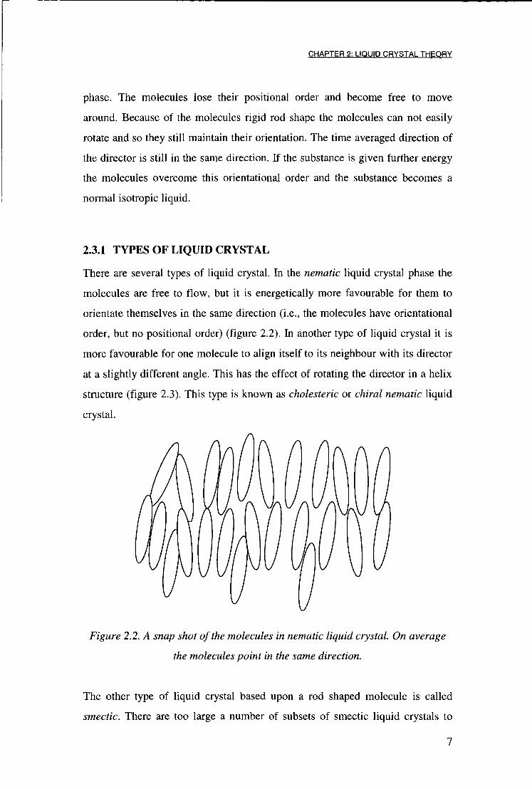
There are several types of liquid crystal. In the nematic liquid crystal phase the
molecules are free to flow, but it is energetically more favourable for them to
orientate themselves in the same direction (i.e., the molecules have orientational
order, but no positional order) (figure 2.2). In another type of liquid crystal it is
more favourable for one molecule to align itself to its neighbour with its director
at a slightly different angle. This has the effect of rotating the director in a helix
structure (figure 2.3). This type is known as cholesteric or chiral nematic liquid
crystal.
I I Figure 2.2. A snap shot of the molecules in nematic liquid crystal. On average
the molecules point in the same direction.
The other type of liquid crystal based upon a rod shaped molecule is called
smectic. There are too large a number of subsets of smectic liquid crystals to
7
CHAPTER 2: LIQUID C R Y S T A L T H E O R Y
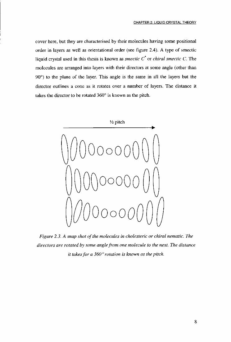
cover here, but they are characterised by their molecules having some positional
order in layers as well as orientational order (see figure 2.4). A type of smectic
liquid crystal used in this thesis is known as smectic C* or chiral smectic C. The
molecules are arranged into layers with their directors at some angle (other than
90°) to the plane of the layer. This angle is the same in all the layers but the
director outlines a cone as it rotates over a number of layers. The distance it
takes the director to be rotated 360° is known as the pitch.
Vi pitch •
A
JOOooooOO A A A
O00°°°oo
tfOOooooOOfl Figure 2.3. A snap shot of the molecules in cholesteric or chiral nematic. The
directors are rotated by some angle from one molecule to the next. The distance
it takes for a 360° rotation is known as the pitch.
8
CHAPTER 2: LIQUID C R Y S T A L T H E O R Y
VJ W A W \J VJvy u
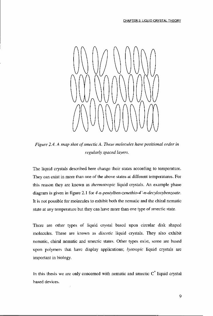
Figure 2.4. A snap shot of smectic A. These molecules have positional order in
regularly spaced layers.
The liquid crystals described here change their states according to temperature.
They can exist in more than one of the above states at different temperatures. For
this reason they are known as thermotropic liquid crystals. An example phase
diagram is given in figure 2.1 for 4-n-pentylben-zenethio-4'-n-decyloxybenzoate.
It is not possible for molecules to exhibit both the nematic and the chiral nematic
state at any temperature but they can have more than one type of smectic state.
There are other types of liquid crystal based upon circular disk shaped
molecules. These are known as discotic liquid crystals. They also exhibit
nematic, chiral nematic and smectic states. Other types exist, some are based
upon polymers that have display applications; lyotropic liquid crystals are
important in biology.
In this thesis we are only concerned with nematic and smectic C liquid crystal
based devices.
9
C H A P T E R 2: LIQUID C R Y S T A L T H E O R Y
2.3.2 T H E E F F E C T OF E L E C T R I C F I E L D S ON LIQUID C R Y S T A L S
The molecules used in liquid crystal applications have an overall neutral electric
charge. However, certain atoms within the molecules are more electrophilic
(they attract electrons) than others. This gives the atoms a slight negative electric
charge. I f a liquid crystal molecule has electrophilic and electrophobic (repels
electrons) atoms there will be a permanent electric dipole. If these molecules are
placed in an electric field, the dipole will produce a rotational torque, T,
T = P x E [2.1]
where E is the electric field and P is the dipole moment. This torque rotates the
molecule, aligning its with the electric field. When the electric field is removed
the molecule will return to its original orientation.
In practice, a DC field would cause the liquid crystal cell to degrade. An AC
field is instead applied. When an AC electric field is applied to a molecule, the
field causes electrons to be displaced within the molecule. This displacement of
charge causes an induced dipole moment. In an AC field, equation [2.1] would
have a time average of zero if the dipole was static, but because of the electron
mobility within the molecule, the induced dipole can flip polarity at the same
frequency as the applied AC field (~lkHz) giving a non-zero value for T.
2.3.3 T H E E F F E C T ON L I G H T OF LIQUID C R Y S T A L S
Elongated molecules have different dielectric constants, and hence different
refractive indices, for each of their axes. In an isotropic liquid the effect is
averaged out so the material will be optically isotropic. In crystalline solids, such
as quartz and in liquid crystals, the refractive index for the whole crystal will be
different for light entering in different polarisation states. The crystal is
birefringent. The long axis of the liquid crystal has what is called the
10

CHAPTER 2: LIQUID C R Y S T A L T H E O R Y
extraordinary refractive index, and the two shorter axes have what is called the
ordinary refractive index (figure 2.5).
He
Figure 2.5. The anisotropic rod shaped nature of the liquid crystal molecules
gives rise to their isotropic refractive indices and the molecules' birefringence.
The birefringence of the liquid crystal is defined as
An = n.. - n.. e a
[2.2]
where ne is the extraordinary refractive index and na the ordinary. It is often
useful to think of homogenous liquid crystals as being variable linear
waveplates.
2.3.4 PHASE SHIFTING BY NEMATIC LIQUID C R Y S T A L S
Consider a glass cell of nematic liquid crystal with incident light polarised along
the extraordinary axis. The phase shift, <)), experienced by the incident light
linearly polarised along the extraordinary axis compared to the phase shift along
the ordinary axis as it passes through the liquid crystal of thickness d, wil l be
11
C H A P T E R 2: LIQUID C R Y S T A L T H E O R Y
0 = — d An [2.3] A.
where An is the effective birefringence experienced by the light and X is the
wavelength of the light. An is a function of voltage and is at its maximum when
there is no electric field across the liquid crystal cell. If an electric field is now
applied across the cell, the liquid crystal molecules will be rotated. The light will
experience less of the extraordinary refractive index of the material and the value
of An will decrease. Hence, the phase shift caused by the liquid crystal material
will be different.
Because the liquid crystal is driven by an AC field, it is only possible to drive the
liquid crystal in one direction. To reset the liquid crystal the electric field is
removed and the liquid crystal molecules relax to their original orientation. This
is slow compared to the speed when driven by an electric field and limits the
speed of nematic liquid crystals to typically 40ms for a "K phase shift in the
visible. Nematic liquid crystal can be considered as a waveplate with a variable
retardance.
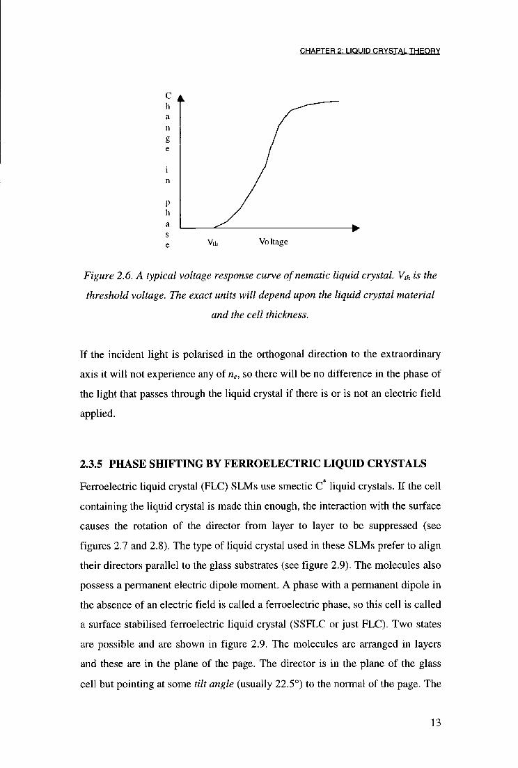
The response of the liquid crystal to an applied electric field is non-linear. Figure
2.6 shows the response of the liquid crystal against potential difference across
the cell. The vertical axis shows the change in phase shift (in arbitrary units) of
light passing through the cell. There is a certain threshold voltage, V th, below
which there is no response. This is important for multiplexing SLMs (see
Chapter 4).
12
CHAPTER 2: LIQUID C R Y S T A L T H E O R Y
g e
n
s e Vth Voltage
Figure 2.6. A typical voltage response curve ofnematic liquid crystal. Vth is the
threshold voltage. The exact units will depend upon the liquid crystal material
and the cell thickness.
If the incident light is polarised in the orthogonal direction to the extraordinary
axis it will not experience any of ne, so there will be no difference in the phase of
the light that passes through the liquid crystal if there is or is not an electric field
applied.
2.3.5 PHASE SHIFTING B Y F E R R O E L E C T R I C LIQUID C R Y S T A L S
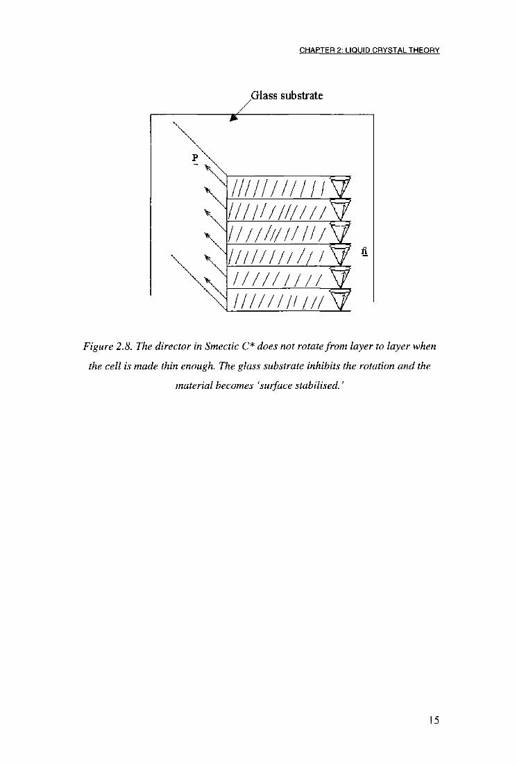
Ferroelectric liquid crystal (FLC) SLMs use smectic C* liquid crystals. If the cell
containing the liquid crystal is made thin enough, the interaction with the surface
causes the rotation of the director from layer to layer to be suppressed (see
figures 2.7 and 2.8). The type of liquid crystal used in these SLMs prefer to align
their directors parallel to the glass substrates (see figure 2.9). The molecules also
possess a permanent electric dipole moment. A phase with a permanent dipole in
the absence of an electric field is called a ferroelectric phase, so this cell is called
a surface stabilised ferroelectric liquid crystal (SSFLC or just FLC). Two states
are possible and are shown in figure 2.9. The molecules are arranged in layers
and these are in the plane of the page. The director is in the plane of the glass
cell but pointing at some tilt angle (usually 22.5°) to the normal of the page. The
13
C H A P T E R 2: LIQUID C R Y S T A L T H E O R Y
electric polarisation is aligned perpendicular to the director and is in the plane of
the page. By changing the polarity of the applied electric field the molecules
rotate round. Looking through the cell, this has the effect of rotating the director
by twice the tilt angle. This is called the switching angle. This is effectively an
electronically rotatable waveplate. By suitable configuration of polarisers, the
FLC SLM can be made to produce either phase modulation or amplitude
modulation.
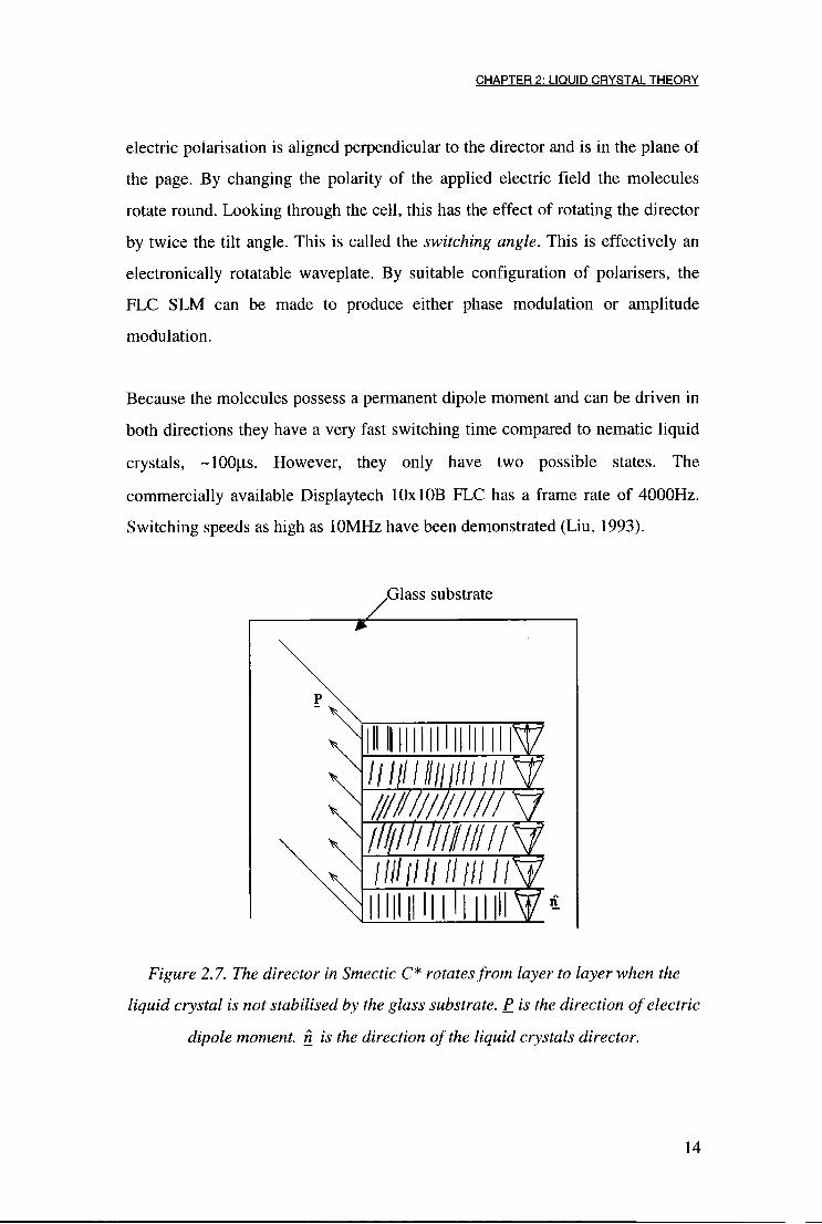
Because the molecules possess a permanent dipole moment and can be driven in
both directions they have a very fast switching time compared to nematic liquid
crystals, ~100|4,s. However, they only have two possible states. The
commercially available Displaytech 10x1 OB FLC has a frame rate of 4000Hz.
Switching speeds as high as 10MHz have been demonstrated (Liu, 1993).
Glass substrate
Ill I III Ml WW illII/IIIII I 111 V 2 / / / / / / / / II HI i i w 2*
Figure 2.7. The director in Smectic C* rotates from layer to layer when the
liquid crystal is not stabilised by the glass substrate. P is the direction of electric
dipole moment, n is the direction of the liquid crystals director.
14
CHAPTER 2: LIQUID C R Y S T A L T H E O R Y
Glass substrate
/ / / / / / / / / / / V 2 mil i ii/i i i i / / / n / / ^ i / / i i / / i i / / \ f
n
Figure 2.8. The director in Smectic C* does not rotate from layer to layer when
the cell is made thin enough. The glass substrate inhibits the rotation and the
material becomes 'surface stabilised.'
15

CHAPTER 2: LIQUID C R Y S T A L T H E O R Y
n
n
Figure 2.9 The SSFLC. The layers of smectic molecules are in the plane of the
page. The director, n , is shown as its projection onto the plane of the page. It is
at an angle of22.5° to the perpendicular of the page's plane. The application of
an electric field causes the switching between the two states.
O F F \ P O L 1
/ O N
P O L 2
Figure 2.10. The alignment of the input and output polarisers with reference to
the switching angle of the FLC needed to attain a phase shift of K when the
retardance of the device is not K and the switching angle is not 90 °. POL I is
the input polariser and POL 2 is the output polariser. ON and OFF represent
the two optical axes of the FLC.
16

CHAPTER 2: LIQUID C R Y S T A L T H E O R Y
As discussed above, FLCs are birefringent and produce a phase shift by an
electrically controlled rotation of the optical axis. The device needs to be placed
between two crossed polarisers, where the axis of the first bisects the two optical
axes states of the FLC (see figure 2.10).
The retardance, T, of the FLC is given by
where d is the thickness of the FLC, A. the wavelength of light, and An the
birefringence of the liquid crystal.
The phase shift produced by the FLC can be calculated using Jones calculus.
There is often an absolute phase term, e1*, in the Jones matrices. Since we are not
interested in the absolute phase, only the difference between the on and off states
of the FLC, this is dropped to simplify the mathematics.
The FLC can be considered as a retarder with its optical axis at angle 9 (the tilt
angle) to the vertical. The FLC is then represented by W
e ^ c o s ^ + e ' ^ s h ^ e •
sin0cos6-e / 2 sinGcosG W = [2.5]
1 sin0cos0-e n sin0cos0 sin 2e + e ! ^cos 2 e
The incident light is vertically polarised and represented by V
0 V = [2.6]
17

C H A P T E R 2: LIQUID C R Y S T A L T H E O R Y
and the output polariser is, P
1 0 P = [2.7]
0 0
The transmitted amplitude, T, is then given by
T = PWV [2.8]
2cos0sin0-e / 2cos0sin0
[2.9] 0
for the Displaytech FLC used in this thesis, r=0.67i and the tilt angle, 0, is
±22.5°.
So we have a phase shift of ±7t/2 with an amplitude of 0.572. The ± refers to the
device in either its 'on' or ' o f f mode. So switching from 'on' to ' o f f , a change
in phase of n is introduced. The transmission is measured in terms of intensity
and is I-0.572I2 = 33%.
2.3.6 F L C O P E R A T E D WITH NO POLARISERS
If we consider the case of an ideal FLC SLM the retardance would be n radians
and the switching angle 90°. In this case no polariser would be needed in the
system. We can consider unpolarised light as the superposition of two incoherent
linearly polarised beams.
T = - i •0.572- e [2.10] 0
18

CHAPTER 2: LIQUID C R Y S T A L T H E O R Y
For r = n and G = ±45°, equation [2.5] becomes
W =
0 ±i'
±i 0 [2.11]
If we first consider the vertical component of the incident light, V, we get
T v = WV [2.12]
±i-
0
[2.13]
The Jones's matrix for horizontally polarised light, H, is
H [2.14]
so
T H = WH [2.15]
0
[2.16]
The FLC rotates the polarisation of the light by 90° (as expected for a half
waveplate with the incident light at 45°). There is still a phase shift of n radians
between the two states.
19

C H A P T E R 2: LIQUID C R Y S T A L T H E O R Y
An alternative method of improving the transmission has been proposed by Neil
and Paige (Neil, 1994) using the FLC with a quarter wave plate and a mirror in
the system. The system still requires a polariser but the transmission is increased.
Warr et. al. (Warr, 1995) increased the throughput of their system by using no
polarisers with a non-ideal FLC. This left a large DC peak in their diffraction
pattern for a O/tc grating. To the author's knowledge, there has not yet been any
assessment of using imperfect FLCs in an adaptive optics system.
2.4 Applications of liquid crystal SLMs
The most common applications of liquid crystal SLMs are displays. These are
usually based upon a slightly modified type of nematic liquid crystal device
called a twisted nematic liquid crystal (TNLC). This was invented in the late
1970's and has revolutionised many display applications. A twisted nematic cell
is made by sandwiching nematic liquid crystal between two glass plates. The
glass plates have rubbing directions1 90° to each other. This causes a gradual
rotation of the director through the cell in a helical structure (see figure 2.11).
Linearly polarised light entering the cell is rotated by this helix and an output
polariser is placed after the cell 90° to the polarisation of the incident light. This
gives the maximum transmission. When an electric field is applied to the cell,
the molecules realign and there is no longer any rotation of the director through
the cell, and hence no rotation of the polarisation. This gives extinction of light.
'The "rubbing direction" is the direction in which the director aligns. It can be made by rubbing a
polymer alignment layer on the glass with a piece of cloth in one direction or by a placing a
chemical deposit on the glass surface.
20

C H A P T E R 2: LIQUID C R Y S T A L T H E O R Y
Figure 2.11. A twisted nematic display. Light enters at the top though a
polariser. When there is no electric field the molecules rotate the plane of
polarisation by 90° and it passes through the second polariser that is orthogonal
to the first. When an electric field is applied there is no rotation and hence no
transmission of light.
Colour displays are created by having either dyes in the liquid crystals or
coloured filters. These produce colour images in a similar way to TVs by having
red, green and blue pixels.
Problems caused by addressing large numbers of pixels have been tackled in
recent years by incorporating thin film transistors (TFT) and other electronics
into the displays to act as switches for the pixels. Another alternative is to build
the SLM on a silicon back plane which also acts as the control electronics (for a
review see (Clark, 1994) and (Johnson, 1993)).
FLCs are not as commonly used in displays. To generate a grey scale temporal
multiplexing is used (Landreth, 1992), i.e., to get a 100 grey levels each picture
frame is divided, temporally, into 100 sub-frames. To get a 25% grey level the
pixel is switched on for 25 sub-frames and off for 75 sub-frames. The eye
integrates this making the pixel appear grey. These devices can be made to be
21

CHAPTER 2: LIQUID C R Y S T A L T H E O R Y
very small, with a resolution in excess of 500 lines per inch (Worboys, 1993)
and are used in applications such as helmet mounted displays.
Both phase modulators and intensity modulators have been constructed using
optically addressed liquid crystal SLMs (OASLM) or liquid crystal light valves
(LCLV) (Efron, 1985 & Moddel, 1987). The liquid crystal is placed onto a
photoconductive layer. The resistance of the layer is dependent on the amount of
light incident on it. This alters the electric field across the liquid crystal cell, and
either gives amplitude or phase modulation (Johnson, 1990) depending upon the
optical configuration of the device. By a suitable choice of photoconducter the
device can be used to convert infrared images into visible images.
All of the devices in this thesis are driven electronically. This is achieved by
either direct drive or multiplexing. Direct drive SLMs have an electrode
connected to each individual pixel. When there is a large number of pixels, it
becomes difficult to individually connect each pixel. Instead, the pixels are
multiplexed. The pixels are activated by selecting the correct row and column.
22
C H A P T E R 2: LIQUID C R Y S T A L T H E O R Y
2.4.1 M U L T I P L E X I N G T H E O R Y
Y l Y2 Y3
XI
X2
X3
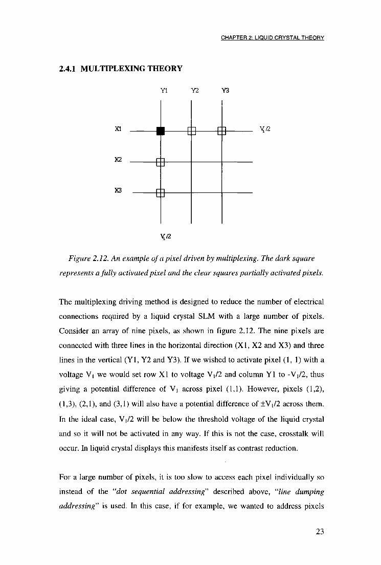
Figure 2.12. An example of a pixel driven by multiplexing. The dark square
represents a fully activated pixel and the clear squares partially activated pixels.
The multiplexing driving method is designed to reduce the number of electrical
connections required by a liquid crystal SLM with a large number of pixels.
Consider an array of nine pixels, as shown in figure 2.12. The nine pixels are
connected with three lines in the horizontal direction ( X I , X2 and X3) and three
lines in the vertical ( Y l , Y2 and Y3). If we wished to activate pixel (1,1) with a
voltage Vi we would set row X I to voltage V|/2 and column Y l to -Vi/2, thus
giving a potential difference of Vi across pixel (1,1). However, pixels (1,2),
(1,3), (2,1), and (3,1) will also have a potential difference of ±V\I2 across them.
In the ideal case, V]/2 will be below the threshold voltage of the liquid crystal
and so it will not be activated in any way. If this is not the case, crosstalk will
occur. In liquid crystal displays this manifests itself as contrast reduction.
For a large number of pixels, it is too slow to access each pixel individually so
instead of the "dot sequential addressing'1'' described above, "line dumping
addressing" is used. In this case, i f for example, we wanted to address pixels
23

C H A P T E R 2: L IQUID C R Y S T A L T H E O R Y
(1,1), (1,3), row X I would be set to V\I2 and both columns Y l and Y3 set to
- V j / 2 . Then row X2 would be set to V i / 2 and the appropriate voltage placed on
the columns we would wish to activate. The rows are known as the common and
the columns as either the segments or simply columns. For a large display, such
as the GEC 64x64 which w i l l be used in chapter 4, the waveforms being applied
to the liquid crystal become very complex (see (Hitachi, 1991) for more details).
This method still has the same crosstalk problem as the dot sequential address
technique.
2.5 Summary
This chapter has covered the basics of liquid crystal theory. The two types of
l iquid crystal, nematic and FLC, that are to be used in this thesis have been
described. The effects of an electric f ield and the effects the liquid crystal
molecules have on light have been described. The next chapter w i l l give a brief
review of atmospheric turbulence and conventional adaptive optics.
24

C H A P T E R 3: A T M O S P H E R I C T U R B U L E N C E A N D C O N V E N T I O N A L A D A P T I V E O P T I C S
Chapter 3: Atmospheric Turbulence and
Conventional Adaptive Optics
3.1 Introduction
In the previous chapter, the essential characteristics of l iquid crystals were
described. In this chapter, there w i l l be a review of conventional adaptive optics
and the causes of atmospheric turbulence. Adaptive optics in non-astronomical
applications and other sources of aberrations that potentially require adaptive
optics are discussed.
3.1.1 THE FUNCTION OF AN ASTRONOMICAL TELESCOPE AND
HISTORY OF ADAPTIVE OPTICS
The purpose of an imaging telescope is to collect as much celestial radiation as
possible and focus this into an image with the highest resolution as possible. The
diameter of the telescope is the fundamental l imit of both of these. The light
gathering power is dictated by the collecting area of the primary mirror. The
resolution of any optical imaging device is limited by diffraction. The so called
Rayleigh criterion defined when two points, separated by an angle OR, can be
resolved, is given by
where D is the diameter of the imaging device, in this case the diameter of the
telescope's aperture, and A, is the wavelength of the incident light.
Increasing D increases the resolution of the telescope. However, turbulence in
the Earth's atmosphere limits the resolution to about 1 " which is equivalent to
D=10-20cm in the visible. This was noticed as far back as Newton, (Newton,
1704) who in his book Opticks could see no possible solution to the problem:
0 1.22 D [3.1]
25

C H A P T E R 3: A T M O S P H E R I C T U R B U L E N C E A N D C O N V E N T I O N A L A D A P T I V E O P T I C S
"If the Theory of making Telescopes could at length be fully brought into Practice, yet there would be certain Bounds beyond which Telescopes could not perform. For the Air through which we look upon the Stars, is in a perpetual Tremor; as may be seen by the tremulous Motion of Shadows cast from high Towers, and by the twinkling of the fix 'd Stars. But these Stars do not twinkle when viewed through Telescopes which have large apertures. For the Rays of Light which pass through divers parts of the aperture, tremble each of them apart, and by means of their various and sometimes contrary Tremors, fall at one and the same time upon different points of the Eye, and their trembling Motions are quick and confused to be perceived severally. And all these illuminated Points constitute one broad lucid Point, composed of those many trembling Points confusedly and insensibly mixed with one another by very short and swift Tremors, and thereby cause the Star to appear broader than it is, and without any trembling of the whole...
The only Remedy is a most serene and quiet Air, such as may perhaps be found
on the tops of the highest Mountains above the grosser Clouds. "
In 1953 Babcock (Babcock, 1953) first proposed using what is now called
adaptive optics to compensate for the atmosphere and restore the resolution to
the diffraction l imit
"If we had a means of continually measuring the deviation of rays from all parts
of the mirror, and of amplifying and feeding back this information so as to
correct locally the figure of the mirror to the schlieren pattern, we could expect
to compensate both for the seeing and any inherent imperfections of optical
figure."
Babcock's attempts to implement his idea were thwarted by the technology
limitations of the time. Adaptive optics was neglected until the 1970's when, the
26
C H A P T E R 3: A T M O S P H E R I C T U R B U L E N C E A N D C O N V E N T I O N A L A D A P T I V E O P T I C S
idea was resurrected with limited success (Buffington, 1976; Buffington, 1977;
Hardy, 1976). A large input to adaptive optics technology occurred at the end of
the cold war when US military adaptive optics systems became de-classified.
These systems were designed for observing satellites, as well as focusing laser
beam direct energy weapons as part of the strategic defence initiative (SDI) or
"Star Wars."
In 1989 one of the first civilian astronomical adaptive optics system was
constructed called COME-ON. This provided correction for a small telescope
(Rousset, 1990) and later a 3.6m telescope (Rigaut, 1991). Since then a number
of other systems have been constructed. The upsurge in interest has come about
because of an improvement in wavefront sensing technology; a shift into the
infra-red as the wavelength of interest where the aberrations are easier to correct;
and the use of laser guide stars (Foy, 1985).
3.1.2 TERMINOLOGY
It is important to distinguish between adaptive optics and the closely related f ie ld
of active optics. Adaptive optics is used to compensate for rapidly varying
aberrations (>=10Hz), whilst active optics is used to correct for deformations in
the actual telescope. These deformations can arise f rom thermal expansions,
mechanical strains, etc. in the telescope's optics and structure. They typically
have a frequency of < l H z . Active optics sometimes uses the telescope's primary
mirror as a deformable mirror such as in the ESO-NTT and the 10 metre Keck
telescope. Adaptive optics usually uses a small deformable mirror.
I f a system employs any feedback it w i l l be called closed loop. I f there is no
feedback it w i l l be called open loop.
27

C H A P T E R 3; A T M O S P H E R I C T U R B U L E N C E A N D C O N V E N T I O N A L A D A P T I V E O P T I C S
3.2 Wavefront Distortions Caused by the Atmosphere
The Earth's atmosphere is approximately 20km thick. At sea level the
atmospheric pressure is approximately 105Pa and tends towards zero as height is
increased. The change in pressure effects the refractive index of the air. This is
1.0003 at sea levels and tends toward unity with height. As the sun rises and sets,
turbulence is created in the atmosphere. This comes f rom the differences in the
heating rates of the Earth's different surfaces (such as water, soil, and rock)
causing convection currents which mix with air of different regions causing
eddies. This turbulence is in several layers. I f the turbulence were absent,
incident light with a plane wave would propagate through the atmosphere
unaberrated. However, the turbulence causes changes in pressure and hence
refractive index. These changes in refractive index cause the optical path length
of light passing through to change (see figure 3.1). Although the changes in
refractive index are small, the fact that light passes through several kilometres of
air means that the change in path length is of the order of micrometres when it
reaches the Earth's surface.
Incident plane wavefront f rom star
"^---Turbulent atmosphere
\ \ \ \ \ \ \ \ \ \ \ \ \ \ \ \ \ \ \ \ \ \ \ \ \ \ \ \ \ \ \ \ \ \ \ \ \ \ \ \ \ \ '
Aberrated wavefront
Ground level
Figure 3.1. As the plane wavefront from the star enters the atmosphere, it
becomes aberrated.
28
C H A P T E R 3: A T M O S P H E R I C T U R B U L E N C E A N D C O N V E N T I O N A L A D A P T I V E O P T I C S
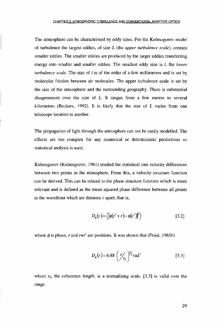
The atmosphere can be characterised by eddy sizes. For the Kolmogorov model
of turbulence the largest eddies, of size L (the upper turbulence scale), contain
smaller eddies. The smaller eddies are produced by the larger eddies transferring
energy into smaller and smaller eddies. The smallest eddy size is /, the lower
turbulence scale. The size of / is of the order of a few millimetres and is set by
molecular friction between air molecules. The upper turbulence scale is set by
the size of the atmosphere and the surrounding geography. There is substantial
disagreement over the size of L. It ranges f rom a few metres to several
kilometres (Beckers, 1992). It is likely that the size of L varies f rom one
telescope location to another.
The propagation of light through the atmosphere can not be easily modelled. The
effects are too complex for any numerical or deterministic predictions so
statistical analysis is used.
Kolmogorov (Kolmogorov, 1961) studied the statistical rms velocity differences
between two points in the atmosphere. From this, a velocity structure function
can be derived. This can be related to the phase structure function which is more
relevant and is defined as the mean squared phase difference between all points
in the wavefront which are distance r apart, that is,
where (j> is phase, r and r+r are positions. It was shown that (Fried, 1965b)
where r 0 , the coherence length, is a normalising scale. [3.3] is valid over the
range
D,(r)=(W + r U ( r ' ) f )
Z U r ) = 6.88 rad o J
[3.3]
29

C H A P T E R 3: A T M O S P H E R I C T U R B U L E N C E A N D C O N V E N T I O N A L A D A P T I V E O P T I C S
l<r<L [3.4]
Fried's coherence length, ro, is an important parameter in adaptive optics; it is a
measure of the severity of the atmospheric turbulence. Fried found that the
maximum diameter of a telescope before atmospheric turbulence limited the
performance is given by (Fried, 1965a)
ro = 0.423k 2 s e c ( ( 3 ) j c 2
n ( h ) d h [3.5]
where ^ is the total path length through the atmosphere, 0 is the zenith angle, h is
the height, C n
2(/i) is known as the refractive index structure constant and k=2n/A,,
where A is wavelength. This is a measure of the strength of the turbulence.
C*(h) varies with height, geographical location and time (with a period of
hours). There is no accurate model of C 2 (h) at present although several authors
have developed approximate models (Hufnagel, 1974; Ulrich, 1988). I f however,
C 2 ( / t ) is approximated to a constant and P=0, it can be related to ro via
f ( \ 2 \
r 0 =1.68 2n
y A. J J
[3.6]
r 0 can also be defined as the diameter of an aperture over which the wavefront
phase variance is equal to 1 radians .
In this thesis r 0 w i l l be taken at (3=0° and A=0.5(0.m unless otherwise stated. Wi th
these parameters it equals approximately 10 - 20cm. This means that, with no
correction for the atmospheric turbulence, the 10 metre Keck telescope has the
same resolution as a 10cm telescope. The atmosphere limits the Keck telescope
to a 100 t h of its diffraction performance.
30

C H A P T E R 3: A T M O S P H E R I C T U R B U L E N C E A N D C O N V E N T I O N A L A D A P T I V E O P T I C S
3.2.1 INTENSITY VARIATIONS
As Sir Isaac Newton pointed out (see §3.1.1) intensity variations, or
scintillations, can be seen with the naked eye as star twinkling. In a telescope
with a larger aperture, this effect is averaged out and it becomes of secondary
importance. There has been little study of intensity variations for adaptive optics
and it is usually ignored. It has been suggested that intensity correction may be
required to image extra-solar planetary systems where the brightness of the
scintillations of the stars drown out the planet orbiting its barycentre. Love and
Gourlay (Love, 1996) describe a method using liquid crystals to do this. For
large telescopes, the phase aberrations are of more importance.
3.2.2 TEMPORAL VARIATIONS
The rate of change of the wavefront distortion depends predominantly upon the
wind velocity. Since the wind is moving with different velocities (magnitude and
direction) depending upon height, a typical value for vw is hard to define. It is
usually taken to be between 5 and 20ms"1.
For a closed loop system to correct turbulence Greenwood (Greenwood, 1977)
calculated the system must work at frequency o f / 0 or higher, /o is known as the
Greenwood frequency and is given by
0.4v w f , o
[3.7]
3.2.3 TEMPORAL POWER SPECTRUM
The temporal power spectrum of atmospheric turbulence is given by (Conan,
1995)
31

C H A P T E R 3: A T M O S P H E R I C T U R B U L E N C E A N D C O N V E N T I O N A L A D A P T I V E O P T I C S
dh ( r \ f
\ WJ
[3.8]
where / is the frequency and the atmosphere has been approximated to a single
rigid layer. This model is not valid as /tends towards zero.
3.2.4 WAVELENGTH DEPENDENCE OF ATMOSPHERIC
TURBULENCE
It can be seen f rom [3.5] that ro, and hence atmospheric turbulence, has a
wavelength dependence (ro A 6 / 5 ) . In the visible, ro is approximately 10-20cm
but this increases with increasing wavelength. Table 3.1 shows typical values for
ro and/o for various wavelengths.
Wavelength / | i m ro /cm /o /Hz
0.5 20 28
1.6 81 16
2.2 118 13
5.0 317 9
Table 3.1. Typical values for ro and fo at various wavelengths. The values chosen
for [3.7] were vw=5ms'' and £=-10km. The wavelengths chosen are viable
transmission windows in the atmosphere.
Because of the increase in ro and decrease in/o with A,, it is easier to construct an
adaptive optics system that works in the infrared.
32
C H A P T E R 3: A T M O S P H E R I C T U R B U L E N C E A N D C O N V E N T I O N A L A D A P T I V E O P T I C S
3.2.5 ZERNIKE MODES AND THE REPRESENTATION OF THE
SPATIAL DISTORTIONS OF THE WAVEFRONTS
It is often useful to describe the phase aberrations in the atmosphere in terms of
Zernike polynomials, Z/p.Q), where j denotes the f h polynomial, p is the radial
co-ordinate in units of the aperture radius, and 8 is the angular co-ordinate.
Zernike polynomials are an orthogonal set of basis functions that can be used to
describe monochromatic aberrations found in optics. The phase aberration is
then
where Oj is the amplitude of the j Zernike mode.
The polynomials were originally used to describe the aberrations in standard
optics where most of the aberrations occur towards the edge. The means that to
describe the atmosphere, where the aberrations are not at the edge of the
telescope but uniformly spread over the whole aperture, a large number of terms
are required. However, most of the power is contained in the low order modes.
The individual polynomials can be derived f rom an expansion of
(Kp,e)=yvz,(p,e) [3.9]
2 e V en; (p^)=V^+T/? ; (p)V2cos(me) m * 0 [3.10]
Z o d d j (p, 0) = V ^ H * ; (p X/2 sin (ml i6) m*0 [3.11]
Z y . (p ,0)=V^TTi?„ o (p) m = 0 [3.12]
where
33

C H A P T E R 3: A T M O S P H E R I C T U R B U L E N C E A N D C O N V E N T I O N A L A D A P T I V E O P T I C S
K ( p ) = t -.v=0
(-iy(n-s) v n~2s
n + m ^ n — m^ [3.13]
— s
n and m are integers, m < n and n-\m\ = even, j is the mode ordering number and
is a function of n and m. The first few terms are shown in table 3.2.
Depending upon the exact definition of j the order of the Zernike polynomials
changes f rom author to author. In this thesis Z 8 is spherical aberration and the
modes for m=3, n=3 come after this.
34

C H A P T E R 3: A T M O S P H E R I C T U R B U L E N C E A N D C O N V E N T I O N A L A D A P T I V E O P T I C S
Azimuthal frequency m
Radial
Degree n
0 1 2
0
1
Z 0 = l
Piston
0
1 Zi=2/xos(0)
Z 2=2psin(0)
Tip/t i l t
2 Z 3 = V3(2p 2 - l )
Defocus
Z 4 = V 6 p 2 sin(26)
Z 5 = Vop 2 cos(29)
Astigmatism
3 Z 6 = V 8 ( 3 p 3 - 2 p ) s i n ( 0 )
Z 7 =V8(3p 3 -2p )cos (e )
Coma
4 Z 8 = V 5 ( 6 p 4 - 6 p 2 + l )
Spherical
Table 3.2. Zernike polynomials
For the j mode corrected by an adaptive optics system, Nol l (Noll , 1976)
calculated the residual variance, o 2 , and these are shown in table 3.3.
35

C H A P T E R 3: A T M O S P H E R I C T U R B U L E N C E A N D C O N V E N T I O N A L A D A P T I V E O P T I C S
Mode Residual Error /radians2
0 1.0299(D/r 0) 5 / 3
1 0 .582(D/r 0 ) 5 / 3
2 0.134(Z)/r 0) 5 / 3 Tip/t i l t removed
3 0.111 ( D / r 0 f 3 Defocus removed
4 0.0880(Z)/r 0) 5 / 3
5 0.0648(D/r 0 ) 5 / 3 Astigmatism removed
6 0.0587(D/r 0 ) 5 / 3
7 0.0525(D/r 0 ) 5 / 3 Coma removed
8 0.0463(D/r 0 ) 5 / 3 Spherical removed
Table 3.3 Residual wavefront errors after correction ofZernike modes. Mode 0
is the wavefront error before correction.
For a large j
a 2 « 0 . 2 9 4 4 r S / 2 { % j [3.14]
From table 3.3 and equation [3.14] it is clear that most of the turbulence power is
concentrated in the first few modes.
In this thesis, the Strehl ratio is defined as the ratio of the peak intensity of the
image of a point source to the peak intensity of the diffraction limited image of
the same point source. For a a 2 « 1 it can be approximated to
SR = e~°2 [3.15]
36

C H A P T E R 3: A T M O S P H E R I C T U R B U L E N C E A N D C O N V E N T I O N A L A D A P T I V E O P T I C S
3.3 Conventional Adaptive Optics
3.3.1 THE NEED FOR ADAPTIVE OPTICS
The need for adaptive optics can be see when the imaging of an object, 0(x,y), is
imaged through the atmosphere's instantaneous phase function <p(x,y). The
complex amplitude of the atmosphere function is
A(x,y) = A0e»lx'y) [3.16]
where Ao is the modulus of amplitude (and is assumed to be constant here). The
point spread function is then the square modulus of the Fourier transform (FT) of
A
P(p,q) = \FT(A(x,y)f [3.17]
p and q are the spatial frequency co-ordinates. The intensity in the image plane is
then
I{p,q) = 0{p,q)®P{p,q) [3.18]
= FT(FT(0(p,q))FT(P(p,q))) [3.19]
where ® indicates the convolution operator.
Because the intensity is the square of the modulus of the complex amplitude
information about the phase is lost and so the atmospheric phase function can
not be determined f rom the intensity pattern alone.
37
C H A P T E R 3: A T M O S P H E R I C T U R B U L E N C E A N D C O N V E N T I O N A L A D A P T I V E O P T I C S
3.3.2 PHASE CONJUGATION
Conventional and liquid crystal adaptive optics, both use the principle of phase
conjugation to perform the correction of the aberrated wavefront. I f we consider
an incident wavefront with a phase error of a that has been introduced by the
atmosphere, then the wavefront is represented by
ae~ia [3.20]
where a is the amplitude. I f the conjugate of the phase, e+,a, is multiplied by
[3.20] the phase error is now zero. This phase conjugate is applied to the
wavefront by changing the optical path length through which the light travels.
This can be by either deforming a mirror or, for example, by using liquid
crystals. Using a deformable mirror is the conventional method in adaptive
optics. In order to apply the phase conjugate is it necessary to have a wavefront
sensor to measure the phase error.
3.4 Deformable Mirrors
Corrective elements for modern telescopes usually fal l into two groups of
deformable mirrors (DMs):
• Segmented mirrors such as M A R T I N I (Doel, 1990), ELECTRA (Buscher,
1997)
• Continuous face plate mirrors such as COME-ON (Rigaut, 1991)
The simplest design is the piston only segmented mirror. Each mirror segment is
driven with one degree of freedom, usually by piezo-electric crystals. The more
complex variety have 3 degrees of freedom: piston, tip and til t . These mirrors
more closely f i t the incident wavefront. Both types suffer f rom diffraction and
energy loss caused by the gaps between each mirror segment.
38

C H A P T E R 3: A T M O S P H E R I C T U R B U L E N C E A N D C O N V E N T I O N A L A D A P T I V E O P T I C S
Continuous face plate mirrors consist of a continuous deformable mirror placed
over driving actuators. There are several different methods of driving such a
mirror:
1. Discrete positional actuators. Piezo-electric crystals are placed behind the
mirror and push or pull the mirror into the desired shape.
2. Discrete force actuators. These are like the discrete positional actuators but a
non-contact force such as an electric field drives the mirror.
3. Bimorph mirrors. A sheet of piezo-electric crystal is bonded to the rear of the
mirror. Application of an electric field causes the piezo-electric sheet to bend.
4. Micro-mirrors. These mirrors are semiconductor devices. They are
manufactured by etching a silicon wafer. They are similar to type 2 above but
are only ~ l c m across. To the author's knowledge they have not yet been
implemented in an astronomical adaptive optics system.
Although there is no optical power loss because there are no segmented elements
causing diffraction and absorption, these mirrors have a complex influence
function when an actuator deforms the mirror. This needs to be accurately
measured. They are also more diff icul t to maintain than segmented mirrors
where a damaged section can easily be replaced.
Most types of D M are driven by piezo-electric crystals. These require large
voltages (=500V) to drive them and consume a lot of power (except in the case
of micro mirrors). This makes the drive electronics diff icul t to design and
introduces an unwanted heating effect inside the telescope. The heating effect
can act as a source of aberrations.
39

C H A P T E R 3: ATMOSPHERIC T U R B U L E N C E AND CONVENTIONAL ADAPTIVE O P T I C S
3.5 Wavefront Sensors
Adaptive optics requires a measurement of the wavefront aberration in order to
apply the conjugate to the phase error. There are two basic methods: direct or
indirect wavefront sensing.
Indirect wavefront sensors make no explicit measure of the phase but use some
other measure that is related to it such as image sharpness (Muller, 1974). It is
possible to use a trial and error method with the corrector. Examples are hill
climbing, evolutionary programming and genetic algorithms. In these cases
random variations are introduced into the corrective element by various methods
(see (Fogel, 1994) and (Srinivas, 1994) for an overview of evolutionary
programming and genetic algorithms). The use of such techniques has not yet
been full addressed for adaptive optics although similar work has been done
using these techniques to design diffractive optical elements (Yoshikawa, 1997).
The major drawback is that it can take several hundred generations of solutions
to reach the optimum. The measurement of how well the device is correcting can
be assessed, for example, by measuring the peak intensity of the corrected image.
In multi-dithering techniques, the corrective elements track a temporally varying
phase delay (O'Meara, 1977). This requires the corrective element to sweep
through its range, to maximise the intensity of the image, faster than the
turbulence. By filtering out the high frequency sweeps, the corrector can be made
to follow the time varying phase variations and keep the image intensity at a
maximum.
Image sharpening techniques monitor some sharpness criteria in the image
(Muller, 1974). They usually vary the phase shift of the corrective element to
maximise this criterion. Because of the high speed required for both image
sharpening and multi-dithering they both suffer from limited bandwidth and
limited photons forming the image.
40

CHAPTER 3: ATMOSPHERIC T U R B U L E N C E AND CONVENTIONAL ADAPTIVE O P T I C S
3.5.1 D I R E C T SENSING AND I N T E R F E R O M E T E R S
Direct wavefront sensing techniques will be used in the work of this thesis.
These techniques are usually either interferometric or tilt/focus sensing. One of
the simplest interferometers is the Michelson interferometer. This type of
interferometer requires the aberrated beam to be interfered with an unaberrated
reference beam. This means that the aberration has to be placed inside an arm of
the interferometer and so it can not be used for atmospheric measurements.
A modified type is the shearing interferometer. This is based upon a Mach-
Zehnder interferometer with one mirror slightly tilted. Tyson (Tyson, 1991)
gives a detailed analysis of how shearing interferometers work. Self-referencing
interferometers offer an alternative. An example of such a device is the point
diffraction interferometer that will be used in chapter 5 and the theory behind it
is covered next.
3.5.2 T H E SMARTT OR POINT DIFFRACTION I N T E R F E R O M E T E R
The Point Diffraction Interferometer (PDI) is from a class of interferometers
called common path interferometers. Unlike a Michelson interferometer, where a
separate unaberrated beam is interfered with the test beam, the PDI uses part of
the test beam to generate its own reference beam.
41

CHAPTER 3: ATMOSPHERIC T U R B U L E N C E AND CONVENTIONAL ADAPTIVE OPT ICS
ST.
\ /
I 8
Input aberrated p j J i s c r e e n ^ a n s m i t t e d a n d
wavefront £
reference wave Figure 3.2. A detail of the PDI aperture. The incident light is focused on to the
pinhole with a lens. The zeroth order light passes through the pinhole creating a
reference beam for the higher orders to interfere with.
The basic design is shown in figure 3.2. The device is similar to a spatial filter.
Incident light is focused onto a semi transparent mask. The mask consists of a
transparent pinhole, about the size of the Airy disk of the beam, and this is
surrounded by a semitransparent screen (transmission -0.1%). A lens behind the
mask images the resultant interferogram onto a camera. The light from the zeroth
order passes through the pinhole. This has no high frequencies and so produces
an unaberrated beam. The rest of the light that passed through the
semitransparent screen now interferes with the unaberrated beam.
3.6 The Shack-Hartmann Wavefront Sensor
A Shack-Hartmann wavefront sensor is another type of direct sensor. It consists
of an array of lenses (or lenslets) focused onto a CCD camera. The local tilt of
the wavefront across each of the lens subapertures can be determined form the
position of the image on the CCD camera.
42
CHAPTER 3: ATMOSPHERIC T U R B U L E N C E AND CONVENTIONAL ADAPTIVE OPTICS
OX
CCD chip
Untilted wavefront
Lenslet Tilted wavefront
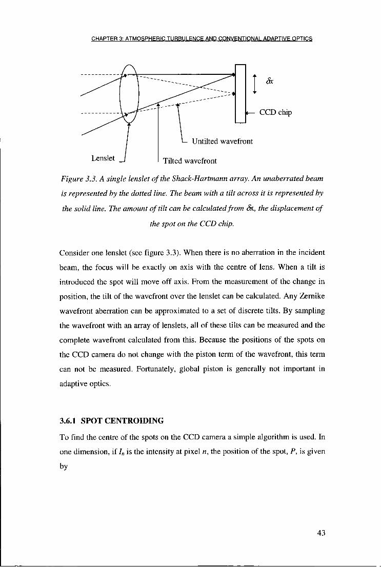
Figure 3.3. A single lenslet of the Shack-Hartmann array. An unaberrated beam
is represented by the dotted line. The beam with a tilt across it is represented by
the solid line. The amount of tilt can be calculated from <5x, the displacement of
the spot on the CCD chip.
Consider one lenslet (see figure 3.3). When there is no aberration in the incident
beam, the focus will be exactly on axis with the centre of lens. When a tilt is
introduced the spot will move off axis. From the measurement of the change in
position, the tilt of the wavefront over the lenslet can be calculated. Any Zernike
wavefront aberration can be approximated to a set of discrete tilts. By sampling
the wavefront with an array of lenslets, all of these tilts can be measured and the
complete wavefront calculated from this. Because the positions of the spots on
the CCD camera do not change with the piston term of the wavefront, this term
can not be measured. Fortunately, global piston is generally not important in
adaptive optics.
3.6.1 SPOT CENTROIDING
To find the centre of the spots on the CCD camera a simple algorithm is used. In
one dimension, i f /„ is the intensity at pixel n, the position of the spot, P, is given
by
43
C H A P T E R 3: ATMOSPHERIC T U R B U L E N C E AND CONVENTIONAL ADAPTIVE O P T I C S
m
P = [3.21] m
I ' . n = i
over m pixels. The CCD camera image is divided up into a number of search
squares. The centre of each square corresponds to the unaberrated spot position
of a lenslet. The position of each spot is calculated and the deviation from the
centre stored in an array. [3.21] is prone to error in low signal to noise situations.
A high background noise will cause P to tend towards the edge of the search
square. The signal to noise ratio in a laboratory can be quite high if a laser is
used as the light source, minimising this source of error. In a situation with a
lower signal to noise ratio this algorithm would have to be modified. A simple
thresholding of all the data improves the accuracy of the system.
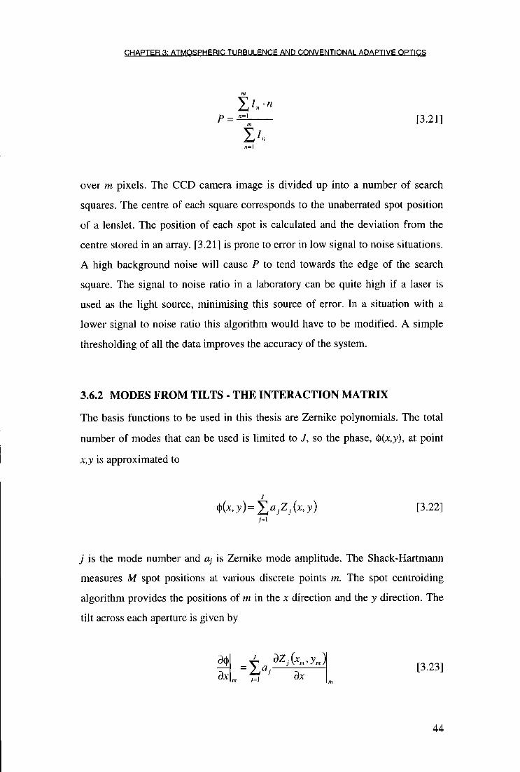
3.6.2 MODES F R O M T I L T S - T H E INTERACTION MATRIX
The basis functions to be used in this thesis are Zernike polynomials. The total
number of modes that can be used is limited to J, so the phase, §(x,y), at point
x,y is approximated to
j is the mode number and a, is Zernike mode amplitude. The Shack-Hartmann
measures M spot positions at various discrete points m. The spot centroiding
algorithm provides the positions of m in the x direction and the y direction. The
tilt across each aperture is given by
j ^(x,y)=y,ajZJ(x,y)
7=1
[3.22]
oZj(xm,ym) a ox ox 7=1 m m
[3.23]
44
C H A P T E R 3: ATMOSPHERIC T U R B U L E N C E AND CONVENTIONAL ADAPTIVE O P T I C S
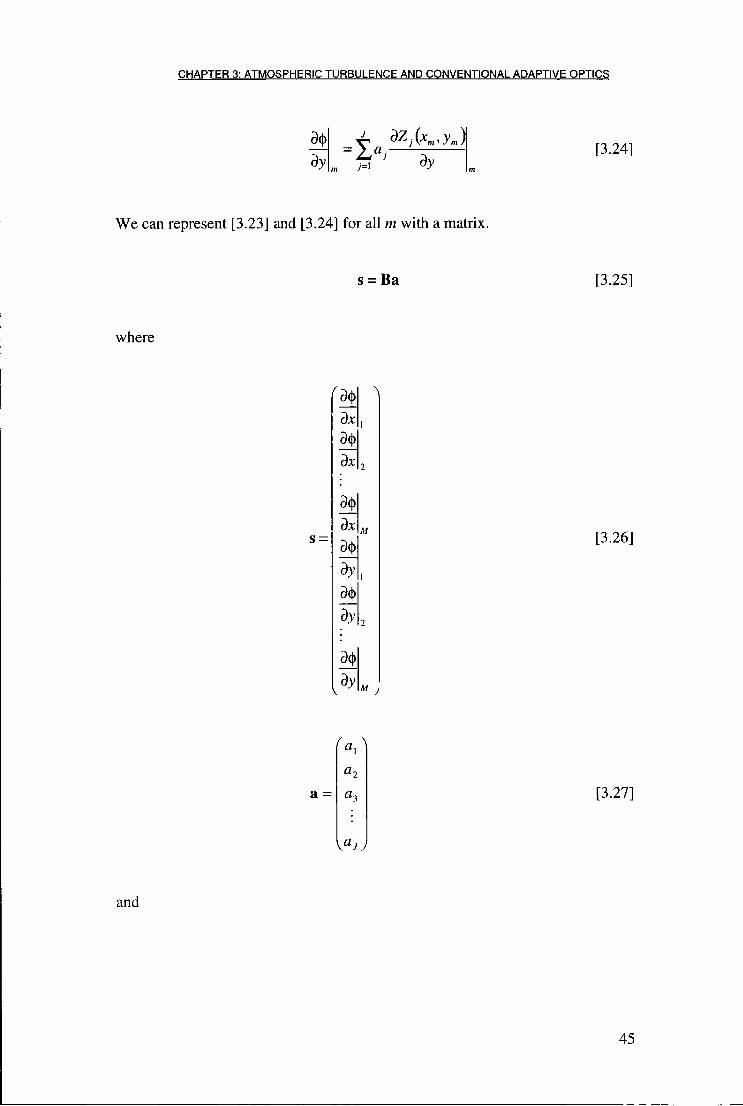
()<)) dv = 1 ^
7=1
[3.24]
We can represent [3.23] and [3.24] for all m with a matrix.
s = Ba [3.25]
where
dx 1
90
2
a<i> dx A /
d§
By 3<K
1
dy 2
90
[ a y M j
[3.26]
a = [3.27]
and
45

C H A P T E R 3: ATMOSPHERIC T U R B U L E N C E AND CONVENTIONAL ADAPTIVE O P T I C S
B
dZ(x,y\ dZ(x, y \ dZ(x, y \
dx dZ(x, y),
, dx dZ(x, y) 2
j dx dZ(x, y \
dx 2 dx 2 dx
dZ(x, y), dZ(x, y)2 dZ(x,y)j
dx dZ(x, y\ dZ(x,y\ dZ(x, y)j
dy
dZ(x, y). dZ(x,y)2 dZ(x, y)j
dy M d y
M
M
[3.28]
B can be calculated off line by calculating the differential for each mode in each
axis for all of the theoretical spot centres. The actual values of element of B
depend upon the size and shape of the lenslet array.
The amplitudes of the Zernike modes can be calculated by rearranging [3.25]
with the pseudoinverse of B.
a = [ (B T B)" 'B T ]s [3.29]
The T indicates the matrix transpose. The pseudoinverse of B is also calculated
off line.
3.6.3 WAVEFRONT CURVATURE
Wavefront curvature sensors are similar in nature to Shack-Hartmann wavefront
sensors except they measure the defocus of a wavefront instead of tilt. Two
measurements of the image are taken, one each axial side of the lens's focus. By
comparing the intensities of the two images, the defocus can be calculated.
Again see Tyson (Tyson, 1991) for a full description. These devices are best
46
C H A P T E R 3: ATMOSPHERIC T U R B U L E N C E AND CONVENTIONAL ADAPTIVE O P T I C S
used with continuous face plate mirrors because the deformation of the mirror closely matches the response of the sensor.
3.7 Binary Adaptive Optics
Binary (or half-wave) adaptive optics offers a simpler alternative to conventional
adaptive optics. Binary adaptive optics was first proposed by Kim et al. (Kim,
1988) for correcting the distortions introduced into the optical system by the
SLM itself. They were using an LCTV as a phase-only SLM to write binary
holograms. The LCTV was not optically flat so they added a binary phase pattern
to the hologram to partially remove the aberration introduced. A Mach-Zehnder
interferometer was used as the wavefront sensor. This was also later repeated by
Tarn et al. (Tarn, 1990) who used a PDI as their wavefront sensor. This system
also used LCTVs. The draw back with these systems was that LCTVs are based
upon nematic liquid crystals that are slower than FLCs, and both systems only
attempt to correct for static aberrations. The idea of binary adaptive optics was
later re-invented by Love et al. (Love, 1993 & 1995) who proposed using a FLC
SLM as the corrective element in a real-time adaptive optics system. Love's
theoretical models were for an atmospheric adaptive optics system using a FLC
SLM.
3.7.1 BINARY ADAPTIVE OPTICS T H E O R Y
When a plane wavefront, sampled by a circular aperture, is focused the resulting
intensity pattern, the PSF, is the well-known Airy disk. When the plane
wavefront becomes aberrated, say by passing through the atmosphere, the PSF is
no longer a perfect Airy disk. Destructive interference reduces the PSF peak
intensity and spreads the light out thereby blurring the image. The concept
behind binary adaptive optics correction is not to completely flatten out the
wavefront to its original form, as in conventional adaptive optics, but to merely
add half a wave to any part of the light that is out of phase. This reduces the
47

CHAPTER 3: ATMOSPHERIC T U R B U L E N C E AND CONVENTIONAL ADAPTIVE O P T I C S
amount of light destructively interfering at the focus and thus partially corrects
the PSF.
The algorithm for binary correction is simple:
When the wavefronts error (modulus X) is greater than half a wavelength apply
a wavefront correction of half a wave.
PLCs are well suited to binary adaptive optics because of their bistable nature. It
has been shown by Love et al. (Love, 1995) that despite only partially correcting
the wavefront an increase in the Strehl ratio from -0% to 40.5% is achievable.
3.7.2 BINARY ADAPTIVE OPTICS AND H I G H E R O R D E R
C O R R E C T I O N WITH F L C S
Unless several devices are cascaded together in an optical system, it is currently
only possible to achieve a two state or bistable SLM with FLCs. With the
suitable configuration of polarisers, FLCs can act as amplitude or phase
modulators. We are only interested in phase modulation at present.
The two states required for binary adaptive optics are -nil and 7T./2, which is
equivalent to saying 0/71 phase shift because we are not interested in the absolute
phase (nor can it be determined). Up to four cascaded devices have been
demonstrated by (Biernacki, 1991), (Freeman, 1992) and (Broomfield,
1995a&b), giving phase shifts of 0, JC/8, 7C/4, 3%/S, nil, 5rc/8, 371/4, and 7rc/8.
Because polarisers need to be incorporated around each device, the transmission
of such a system is prohibitively low (Broomfield quotes a 16dB loss).
48

C H A P T E R 3: ATMOSPHERIC T U R B U L E N C E AND CONVENTIONAL ADAPTIVE O P T I C S
3.8 Non-Astronomical Adaptive Optics Applications
Non-conventional Earth based non-astronomical applications for adaptive optics
has so far been limited. This is mainly because of the high cost of such systems.
There are the possibilities of many more applications. Some of these are
summarised below. Liquid crystals offer the potential for low cost adaptive
optics, although they are not suitable for all applications.
• Space Based Astronomy: Although still an astronomical application this is
included here because it is not an Earth based system and has different
requirements. There is some interest in using some sort of adaptive optics in
the Next Generation Space Telescope (NGST) and in other future space
telescopes (Kuo, 1994). The Hubble space telescope is diffraction limited but
it is limited by the relatively small diameter of its primary mirror (2.4m)
compared to many Earth based telescopes. Placing a larger conventional
mirror into space would be extremely expensive and maybe technically
impossible with the current fleet of Space Shuttles. Some of the current
NGST designs use a primary mirror that folds out like an umbrella. These
mirrors are generally lower quality and so some sort of adaptive optics will
need to be incorporated into the system to compensate for this. There is the
potential of using liquid crystal SLMs for this application. Their lightweight
and robustness makes them potentially suitable for space applications. The
system would be an active optics system, so the liquid crystals slow speed
would not be a disadvantage.
• Military Applications: A large part of the early work on adaptive optics was
done by the US military as part of the Strategic Defence Initiative. These
systems were for ground based satellite observations and laser weapon beam
propagation through the atmosphere.
• Laser welding: There is a need to maintain a fine focus of the beam on the
surface.
49
CHAPTER 3: ATMOSPHERIC T U R B U L E N C E AND CONVENTIONAL ADAPTIVE O P T I C S
• Laser Cavity Applications: An adaptive mirror in a laser cavity echelon can
be used to maintain the correct alignment in the cavity. This is important for
high power applications where the heating of the laser causes the mirrors to
warp. In both this application and the previous, the high power nature would
mean the only corrective device that could be used would be a conventional
deformable mirror.
• Under water imaging: The majority of image degradation when imaging
objects under water comes from scattering from particles in the water.
Adaptive optics may have some applications when imaging in ultra pure
water (e.g. in nuclear power stations).
• Retinal Scanning: When imaging the retina, the resolution is approximately
that of a cone. To image at finer resolutions adaptive optics will be needed.
• Optical Storage Devices: CD based systems already use an adaptive optics
system to maintain focus. It is possible in the future that there will be a need
to use a complete adaptive system, correcting for several Zernike modes. This
may be important in next generation systems, post DVD, where the beam wil l
have to propagate through several layers to reach the desired information, i.e.,
the information is stored in 3 D.
• Hostile Environment Imaging: There is a potential for using adaptive optics in
situations where the environment effects the performance of optics such as in
furnaces. Furnace walls have to be continuously monitored to ensure there is
no soot build up which reduces the heat transfer efficiency. Normal optics
will become stressed when exposed to high temperatures; adaptive optics
could correct for this.
The following chapters will however concentrate on astronomical applications.
50
C H A P T E R 3: ATMOSPHERIC T U R B U L E N C E AND CONVENTIONAL ADAPTIVE OPT ICS
3.9 Summary
In this chapter we have reviewed the sources of aberrations from the atmosphere
and conventional adaptive optics. The statistical Kolmogorov structure of
atmospheric turbulence has been described. The current state of deformable
mirrors and the different types of wavefront sensor have also been reviewed.
Some non-astronomical applications of adaptive optics have been mentioned
although the application of liquid crystal adaptive optics in this thesis will be
towards astronomy.
In the next chapters, the knowledge from the previous two chapters will be used
when constructing liquid crystal adaptive optics systems. The next chapter will
first study a custom built nematic SLM and the possibilities of using this in
adaptive optics.
51

CHAPTER 4: A MULTIPLEXED NEMATIC LIQUID C R Y S T A L SLM
Chapter 4: A Multiplexed Nematic Liquid Crystal
SLM
4.1 Introduction
In this chapter there will be a description of a purpose built 64x64 pixel nematic
liquid crystal SLM. This device was built by GEC, for Durham University and
the Defence Evaluation Research Agency (DERA) for a first attempt at liquid
crystal adaptive optics. This section describes the device, its calibration, and its
performance. Experimental evidence shows there was a major problem when
using the device as a phase only SLM because of its drive electronics.
There are at present several methods used for controlling liquid crystal SLMs.
These include multiplexing, direct drive, active matrix and optical addressing.
Most of the current technological drive behind liquid crystal SLMs is for display
applications. In principle, display technology should be easy to convert to phase
modulating SLMs. Displays such as LCTVs (liquid crystal televisions) and
computer monitors require a large number of pixels. Directly driving each pixel
becomes impossible because of the need to have electrodes going to each
individual pixel. Multiplexing and active matrix are currently used in large
displays. Active matrix displays are currently not suitable to be used as phase
only SLMs for adaptive optics because of their very small f i l l factor (typically
can be as low as -25%). Multiplexing offers a simple driving technique and so
this following section sets out to characterise a custom built device.
4.2 Device Description
The device was based upon standard display technology. It used a 64x64 pixel
glass substrate designed for a twisted nematic liquid crystal display. The drive
electronics are based around the Hitachi HD61203 dot matrix liquid crystal
column driver and the Hitachi HD61203 dot matrix common driver chips. The
device was controlled by a Viglen 80386 IBM compatible PC and software
52

CHAPTER 4: A MULTIPLEXED NEMATIC LIQUID C R Y S T A L SLM
written in Microsoft C. To simplify the device's electronics only the column voltage could be altered, all the row voltages were identical so in effect the device only worked in one dimension. To control the device an array of voltages was sent to the computer's digital to analogue converter (DAC) where this was converted into a serial signal. This signal was amplified and converted back into a digital signal by the liquid crystal drive electronics and fed into the two Hitachi liquid crystal driver chips (see figure 4.1).
ADC
DAC 00
LC SLM
Figure 4.1. The 64x64 SLM's drive electronics block diagram.
The liquid crystal used in the device was E7 produced by Merck (formerly BDH
Ltd.). The main difference between this device and commercially available
devices was that the liquid crystal was not twisted nematic, but parallel aligned.
This enables phase modulation of light without any rotation of its polarisation
state. The device specifications are given in table 4.1.
53

C H A P T E R 4: A MULTIPLEXED NEMATIC LIQUID C R Y S T A L SLM
Specification Value
Liquid crystal Merck E7
Threshold voltage 1.50V
Birefringence An=0.22
Cell thickness 25|J,m
Controllable optical path length 5.5|im
Total theoretical retardance ~nl
Theoretical resolution 7 bit, -A/18 2
Pixel size 400|im
Inter-pixel spacing 40|xm
Pixel f i l l factor 90%
RMS optical flatness (Love, 1994) A/23
Effective number of pixels 64x1
Pixel refresh rate 15ms4
Operating temperature -10°C to +60.5°C
Response time , for A/2 decay (Purvis, 40ms5
1993)
Table 4.1. The specifications of the 64x64 SLM
Although this device is limited in only being able to be driven in one dimension,
it is still useful to assess the capabilities of a multiplexed driven liquid crystal
SLMs for adaptive optics. Multiplexed liquid crystal displays suffer from low
contrast. A similar problem occurs in phase-only modulation. An experiment
was set up to investigate this and to calibrate the liquid crystal for phase versus
voltage applied. The contrast reduction is because of voltage "crosstalk"
'^638.2nm He-Ne 2?t=638.2nm He-Ne. This assumes that the response is uniform over the whole dynamic range, which it is not. 3Measured with a Zygo interferometer, 638.2nm He-Ne 4 This is the speed at which the drive electronics refreshes the S L M . The actual liquid crystal does not work at this speed, to relax from IX to OX phase shift took several seconds 5^=543nm He-Ne
54
CHAPTER 4: A MULTIPLEXED NEMATIC LIQUID C R Y S T A L SLM
between pixels with high applied voltage and pixels with a lower applied voltage.
4.3 Experimental
4.3.1 V O L T A G E W A V E F O R M MEASUREMENTS
The exact voltages being applied to the liquid crystal were investigated. Three
wires were soldered onto the electrical connections of the liquid crystal array on
columns 22 and 42, and row 32. These were then connected to a cathode ray
oscilloscope (CRO). The voltage waveform applied to the liquid crystal could be
measured. By subtracting the voltage waveform from either column 22 or 42
from that of row 32, the potential difference applied across pixels (32,22) or
(32,42) could be measured. Several different voltage waveforms were recorded:
completely off, completely on, half the array on and half the array off, and a
ramp function across the whole array. The individual traces being applied to
each particular row and column were also recorded.
4.3.2 PHASE SHIFT MEASUREMENTS
In order to quantify the crosstalk, the actual phase shifts were measured. It was
assumed that if all of the pixels had the same voltage applied, there would be no
crosstalk between them. Using this assumption a calibration curve for phase shift
versus voltage could be measured.
Nematic liquid crystals are birefringent and so can be treated as normal linear
waveplates but with a variable retardance. When placed between crossed
polarisers, at an angle that bisects the extraordinary and ordinary axis, the SLM
modulates intensity. Using this, the phase shift can be measured indirectly.
When there is a phase shift of (2w+l)7t: the transmitted intensity is at a maximum,
and a minimum when the phase shift is 2nn, where rc=0,l,2.... It was assumed
that the retardance of the liquid crystal would always decrease with increased
potential across the liquid crystal.
55

CHAPTER 4: A MULTIPLEXED NEMATIC LIQUID CRYSTAL SLM
© o oo
CRO
Figure 4.2. The experimental set-up to measure the phase shift induced by the
64x64 SLM. POLl and POL2 are both polarisers at 45 ° and 135° respectively
compared to the optical axis of the SLM, RET is a liquid crystal retarder, SLM is
the 64x64 SLM, PD is a photodiode which measures the transmitted intensity,
and CRO is an oscilloscope.
The experimental set-up is shown in figure 4.2. An additional liquid crystal cell
retarder was required and the voltage across it was altered until there was a
minimum transmission. This was necessary because the retardance of the GEC
64x64 in its 'off state' was not necessarily nn, where n is an integer. The light
source was a 5mW 638.2nm He-Ne laser.
A calibration curve for the SLM was calculated by increasing the voltage applied
across the liquid crystal and recording the minimum and maximum intensity
throughput against voltage.
Once the device was calibrated, the crosstalk could be measured. A fixed voltage
was applied to one half of the device (columns 1-32) whilst the other half (33-
64) had its voltage varied. First of all a voltage that should have induced a In
phase shift according to the calibration curve was imposed on columns 1-32. The
phase shift produced by columns 33-64 was measured as before. This was
repeated for the voltages equivalent to all possible integer values of n phase shift
on columns 1-32. If there was no crosstalk between the two halves, the new
phase/voltage curves generated for columns 33-64 should be identical to the
calibration curve.
RET SLM POL2 LASER POLl
56
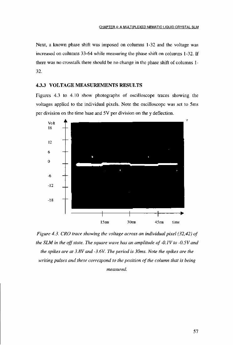
CHAPTER 4: A MULTIPLEXED NEMATIC LIQUID CRYSTAL SLM
Next, a known phase shift was imposed on columns 1-32 and the voltage was
increased on columns 33-64 while measuring the phase shift on columns 1-32. If
there was no crosstalk there should be no change in the phase shift of columns 1-
32.
4.3.3 V O L T A G E MEASUREMENTS R E S U L T S
Figures 4.3 to 4.10 show photographs of oscilloscope traces showing the
voltages applied to the individual pixels. Note the oscilloscope was set to 5ms
per division on the time base and 5V per division on the y deflection.
Volt 18
12
6
0
-6
-12
-18
15ms 30ms 45ms time
Figure 4.3. CRO trace showing the voltage across an individual pixel (32,42) of
the SLM in the off state. The square wave has an amplitude of-0.IV to -0.5V and
the spikes are at 3.8V and -3.6V. The period is 30ms. Note the spikes are the
writing pulses and these correspond to the position of the column that is being
measured.
57

CHAPTER 4: A MULTIPLEXED NEMATIC LIQUID CRYSTAL SLM
15ms 30ms 45ms time
Figure 4.4. CRO trace showing the voltage across an individual pixel when the
whole device is switched fully on. The square wave is ±2V and the spikes (only
seen as dots on this plot) are ±15V. The period is 30ms.
Volt 8
12
0
2
18
15 ms 30ms 45ms time
Figure 4.5. CRO trace showing the voltage applied to a pixel's column
electrode. The device is switched fully on. The square wave is +2. IV to -13V, the
spikes are +4V and -15V, and the period is 30ms.
58

CHAPTER 4: A MULTIPLEXED NEMATIC LIQUID CRYSTAL SLM
15 ms 30ms 45 ms time
Figure 4.6. The same as figure 4.5 but showing the row voltage only (row 32).
The square wave is OVto-llV. Note that there are no spikes on this plot.
Subtracting figure 4.5 gives us figure 4.4.
7 Vo t 18
2
0
12
18
15ms 30ms 45ms time
Figure 4.7. CRO trace showing the voltage across pixel (32,22) with a ramp
function applied across the whole array. The ramp goes from OV to ±2V and the
spikes are + 10.9Vand -77 V. The waveform is an image of what has been
applied to the whole array.
59

Volt 18
12
6
0
-6
-12
-18
CHAPTER 4: A MULTIPLEXED NEMATIC LIQUID CRYSTAL SLM
15ms 30ms 45ms time
Figure 4.8. The same as figure 4.7 but measured from pixel (32,42). The spikes
now have values + 6.9V and -7.0V. The spike's position corresponds to the
position of the column that is been measured.
• *
15ms 30ms 45ms time
Figure 4.9. CRO trace showing the voltage measured from pixel (32,22). A step
function is been applied to the SLM. Columns 1-32 are fully on and columns 33-
64 are o f f . The waveform goes from +2V to -0.1V to -2.2V to -0.2V. The spikes
are + 15V and -15V.
60
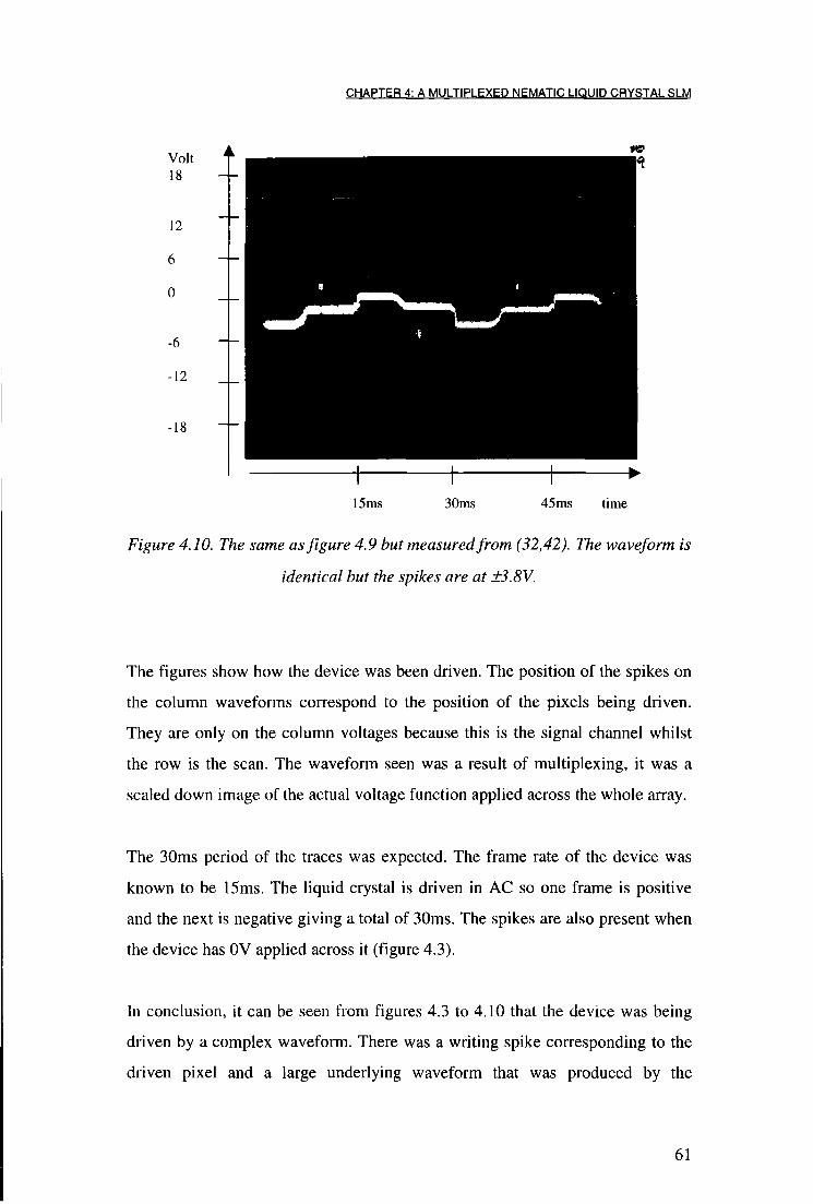
CHAPTER 4: A MULTIPLEXED NEMATIC LIQUID CRYSTAL SLM
Vo t 18
12
0
12
18
15ms 30ms 45ms time
Figure 4.10. The same as figure 4.9 but measured from (32,42). The waveform is
identical but the spikes are at +3.8V.
The figures show how the device was been driven. The position of the spikes on
the column waveforms correspond to the position of the pixels being driven.
They are only on the column voltages because this is the signal channel whilst
the row is the scan. The waveform seen was a result of multiplexing, it was a
scaled down image of the actual voltage function applied across the whole array.
The 30ms period of the traces was expected. The frame rate of the device was
known to be 15ms. The liquid crystal is driven in AC so one frame is positive
and the next is negative giving a total of 30ms. The spikes are also present when
the device has 0V applied across it (figure 4.3).
In conclusion, it can be seen from figures 4.3 to 4.10 that the device was being
driven by a complex waveform. There was a writing spike corresponding to the
driven pixel and a large underlying waveform that was produced by the
61
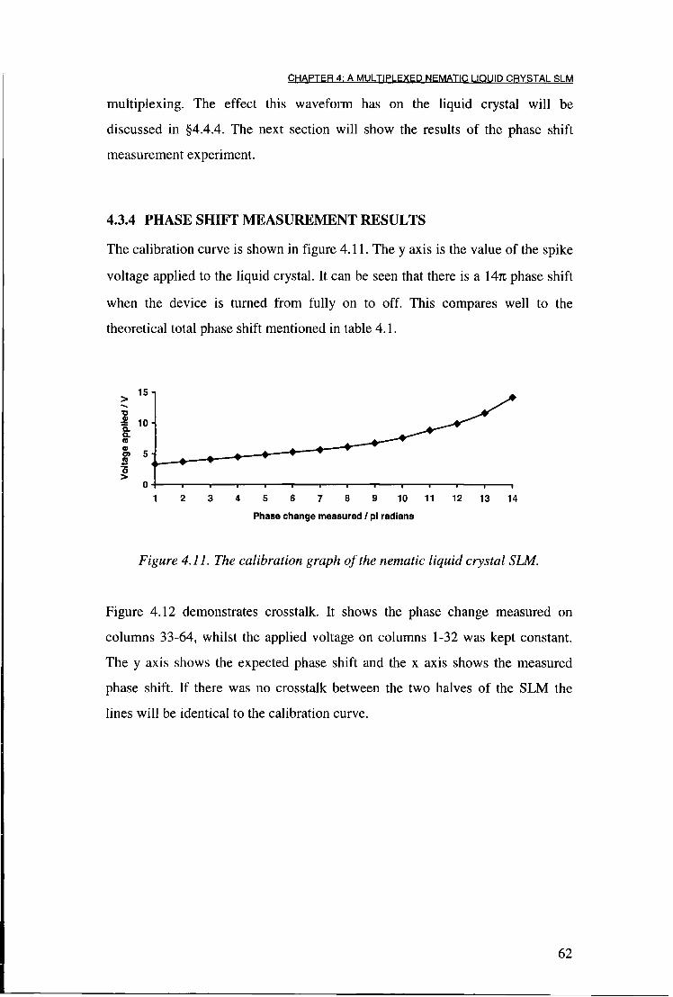
CHAPTER 4: A MULTIPLEXED NEMATIC LIQUID CRYSTAL SLM
multiplexing. The effect this waveform has on the liquid crystal will be discussed in §4.4.4. The next section will show the results of the phase shift measurement experiment.
4.3.4 PHASE SHIFT MEASUREMENT R E S U L T S
The calibration curve is shown in figure 4.11. The y axis is the value of the spike
voltage applied to the liquid crystal. It can be seen that there is a 147C phase shift
when the device is turned from fully on to off. This compares well to the
theoretical total phase shift mentioned in table 4.1.
15
.8 10
0) o> 5
i 6 1 8 9 10 11 12 14 13
Phase change measured / pi radians
Figure 4.11. The calibration graph of the nematic liquid crystal SLM.
Figure 4.12 demonstrates crosstalk. It shows the phase change measured on
columns 33-64, whilst the applied voltage on columns 1-32 was kept constant.
The y axis shows the expected phase shift and the x axis shows the measured
phase shift. If there was no crosstalk between the two halves of the SLM the
lines will be identical to the calibration curve.
62

CHAPTER 4: A MULTIPLEXED NEMATIC LIQUID CRYSTAL SLM
1 pi 16 2 pi
3 pi 14 4 pi
CO 12 CO - * - 5 p i
6 pi 10 7 pi
8 —©—8 pi <o
9 pi 6 10 pi 11 pi in 12 pi in
13 pi 14 pi CAL 1 8 12 13 10 11 14
Actual phase shift measured on pixels 33-64 / pi radians
Figure 4.12. This shows the measured phase shifts produced in columns 33-64 of
the SLM. A fixed phase shift is applied to columns 1-32 (see the legend). The
graph shows the expected phase shift on the vertical axis versus the measured
phase shift on the horizontal axis. The calibration line (CAL in legend) is also
shown.
i p i
16 —•—2 pi —*—3 pi 14
4 pi CO CO 12 —W—5 pi lil
6 pi 10 in
7 pi 8
8 pi is 9 pi 10 pi 11 pi in
12 pi 13 pi
i i i 14 pi 13 1 8 9 11 12 14 Phase shift measured on pixels 1-32 / pi radians
Figure 4.13. The measured phase shift produced in columns 1-32 of the SLM.
Columns 1-32 has the expected phase shift applied that is indicated by the
legend. The phase shift produced by columns 1-32 is shown (x-axis) as the
voltage is varied across columns 33-64 (y-axis).
63

CHAPTER 4: A MULTIPLEXED NEMATIC LIQUID CRYSTAL SLM
Figure 4.13 shows a similar experiment but the phase shift was measured on columns 1-32 whilst the voltages on columns 33-64 where varied. If there was no crosstalk between the two halves of the SLM the lines should be vertical.
It should be noted that the response time of the system was very slow. It took
several seconds to reach a stable state.
For the two graphs in figures 4.12 and 4.13 it is clear that there is significant
crosstalk present between pixels. For example, if a phase shift of n radians is
required on columns 1-32 and a phase shift of 14TT is required on columns 33-64,
the actual applied phase shift is 10ft on columns 1-32 and \2n on columns 33-
64. The actual measured phase shift tends towards some value between the two
theoretically applied values.
4.4 Discussion
The reason for such a large amount of crosstalk error can be seen in figures 4.3
to 4.10. The spikes seen are the writing pulses that activate the individual liquid
crystal pixels. The underlying waveform comes from the multiplex process.
There is a contribution from each pixel to the overall waveform. Only the
writing spike is above the threshold voltage of the liquid crystal. Ideally only the
writing spike should effect the liquid crystal, but the underlying waveform
contributes to the RMS voltage that the liquid crystal experiences and this is
large enough to switch on other liquid crystal pixels partially and produce
crosstalk. Because the waveform models the total pattern applied to the whole
SLM, this waveform has an effect on each pixel. When only a small voltage is
applied to half of the SLM this will lower the RMS voltage across the other half
of the SLM and lower the applied voltage to each pixel.
The writing spike is only 234fis long and so for 14.766ms the liquid crystal pixel
is undriven and will start to relax. As the number of rows is increased, the
writing spike will become shorter and so the actual RMS phase shift of the
64
CHAPTER 4: A MULTIPLEXED NEMATIC LIQUID CRYSTAL SLM
device over one frame will decrease. This limits the number of rows that can be driven in a multiplexed display because the contrast of the display decreases. This will be similar in phase only SLMs.
The effect of this partial pixel activation is common to all multiplexed displays
(Pankove, 1980). If 14TI phase shift is applied to one half of the SLM and Ore
phase shift applied to the other half, there will be an induced unwanted phase
shift in the On half, and \4n half will have a reduced phase shift.
This experiment only looks at the crosstalk between two halves of a 64 pixel
device. It seems logical to assume that a more complex function on the SLM will
also have crosstalk effects. This crosstalk reduces the potential use of the device
as an adaptive optics component when the full dynamic range of the device is
required. It has however been successfully demonstrated by Love et al. (Love,
1994) correcting a tilt in a wavefront when the device was placed in a Zygo
interferometer. He only produced a phase shift of the order of ~1A.. At this level
the crosstalk will be very small. Love did not investigate any effects of crosstalk
in his paper.
Although multiplexing offers an easy way to drive large numbers of pixels it
should be clear that the current display technology used in this device is not
adequate to be adapted to phase only modulation. Other driving techniques for
devices with large number of pixels suffer from poor fill factors because of the
required electrical circuitry, except for optical addressing techniques. Unless
optical addressing techniques are employed, it means other authors claims of
liquid crystal offering a large number of pixels are brought into doubt. By careful
design Meadowlark has produced a 69 pixel direct drive SLM with a high fill
factor. This device is reviewed in chapter 6.
65

CHAPTER 4: A MULTIPLEXED NEMATIC LIQUID CRYSTAL SLM
4.5 Summary
In this chapter a multiplexed nematic liquid crystal SLM has been assessed for
its potential as a phase modulator. The device was only a prototype and was only
driven in one dimension. The device was not intended for use in astronomical
applications and has not been optimised for speed. The important point that this
chapter has shown is that the multiplexed driven liquid crystal SLM could not
accurately cause a desired phase shift over there whole dynamic range and so
was not very suitable for adaptive optics. For this reason it was decided not to
continue with the GEC device, but to use standard commercially available
SLMs. The simplest to use is the FLC device built by Displaytech. This is a
direct drive device and so does not have the problems associated with a
multiplexed device. It is the subject of the next chapter.
66

CHAPTER 5: BINARY CORRECTION WITH A POINT DIFFRACTION INTERFEROMETER
Chapter 5: Binary Correction with a Point
Diffraction Interferometer
5.1 Introduction
This chapter is concerned with using an FLC SLM as a corrective element in an
adaptive optics system. An FLC SLM is capable of 'binary adaptive optics'.
This is the simplest method of providing correction with a liquid crystal device.
The wavefront sensor is a Smartt or point diffraction interferometer (PDI). The
PDI has been chosen in an attempt to reduce the computational overheads that
are commonly found in wavefront sensors, e.g. the Shack-Hartmann, and
shearing interferometer.
A simple phase unwrapping algorithm is developed and the validity of this is
confirmed with computer modelling of the PDI/FLC system. The possibilities of
future improvements are also explored which could make the system into a
viable high speed adaptive optics system with astronomical applications among
others.
5.2 Background
Binary adaptive optics aims to provide correction for an aberrated wavefront
where conventional adaptive optics can not. This may be because of the high
cost of conventional adaptive optics or other factors such as its bulky size and
computational power requirements. Conventional adaptive optics can be broken
down into three areas:
1. Wavefront sensing
2. Computer/control hardware
3. Deformable mirrors
67
CHAPTER 5: BINARY CORRECTION WITH A POINT DIFFRACTION INTERFEROMETER
To produce a low cost system, it is important to carefully balance each part of
the system. It has already been said that liquid crystals offer a lower cost
alternative to deformable mirrors. The price of the wavefront sensor and
computer hardware must also be taken into account. In this thesis all of the real
time computation will be on an IBM compatible PC with a C40 DSP image
processor.
Currently, the most commonly used wavefront sensor in the adaptive optics
community is the Shack-Hartmann wavefront sensor. Conceptually, this is one
of the simplest designs, which may partly be the cause of its current popularity.
However, the optical and conceptual simplicities are offset by the computational
burden of calculating the phase. In chapters 5 and 6 we will demonstrate that a
simplified Shack-Hartmann system can be run at a reasonably high speed on a
single C40 and an IBM compatible PC if several criteria are relaxed. This system
is still complex and slow compared to that which could be achieved with a
conventional interferometer. However the need for a reference arm prohibits the
use of such a sensor.
The other wavefront sensor commonly used is the shearing interferometer. These
devices are still, however, computationally expensive and require two
measurements to calculate the phase. Other more novel sensors exist such as
wavefront inversion interferometers (Spektor, 1995), but these still require
complex calculations to determine the wavefronts.
An example of a conventional Shack-Hartmann system's computational
requirements is the ELECTRA system at Durham. This uses 9 TMS320C40
DSPs on a VME bus, a SUN Sparcstation 10 and a Silicon Graphics Indigo-2
workstation to decode the information from a Shack-Hartmann wavefront sensor
and to control a 76 element tip/tilt/piston segmented mirror. The price of this
system will clearly be more expensive than a liquid crystal SLM and so would
not fulfil the criterion of a low cost adaptive optics system that this thesis sets
68

CHAPTER 5: BINARY CORRECTION WITH A POINT DIFFRACTION INTERFEROMETER
out to demonstrate. The PDI offers a low cost alternative to the above systems. It
does not completely determine the phase but this is not important in binary
adaptive optics.
5.2.1 STANDARD R E F E R E N C E ARM I N T E R F E R O M E T R I C
TECHNIQUES
The potential performance of an F L C SLM in binary adaptive optics systems has
been demonstrated using conventional interferometers for static correction.
Thomas (Thomas, 1993) used a 128 by 128 device in a Mach-Zehnder
interferometer to statically correct for an aberrated piece of glass. Thomas also
cascades two devices together producing a higher order correction (quarter wave
correction). This was followed up by Broomfield et al. (Broomfield, 1995a & b)
with a four level system (eighth wave correction). Both of these systems have
transmissions that are too low for astronomical purposes. The nematic LCTVs
system of Kim et al. (Kim, 1988) also worked with a conventional
interferometer.
None of the above authors have demonstrated any real time capabilities. They
only corrected for static aberrations.
5.3 Theoretical Considerations
5.3.1 T H E SMARTT OR POINT DIFFRACTION I N T E R F E R O M E T E R
The theory behind the PDI was described in chapter 3. Because it is a self
referencing interferometer it is suitable to use in binary adaptive optics with
astronomical sources. Figure 5.1 shows an example interferogram produced by
the PDI. The aberration was produced by using a singlet lens that introduced
spherical aberration into the system, shown in figure 5.2. The square pattern is
the FLC. Figure 5.3 shows the same interferogram but with some of the F L C
pixels activated to remove the dark fringe. Figure 5.4 shows an interferogram
69

CHAPTER 5: BINARY CORRECTION WITH A POINT DIFFRACTION INTERFEROMETER
with no spherical aberration but a chequered pattern on the FLC (i.e., half the pixels are on and half are off, like a chess board.)
t m •c Hi
. « -
i l l H • • K •> mm
i
K
Figure 5.1. An example of the PDl's interferogram. The FLC SLM has been
placed in front of the PDI, hence the square aperture. The FLC's interpixel gaps
are clearly visible as the dark cross pattern. The dark fringe is produced by an
aberration introduced into the system to demonstrate the PDI. If there were no
aberrations present there would be no fringes visible.
L2 FLC L I PDI CCD
W V
Figure 5.2. The experimental set-up to produce the sample interferogram in
figure 5.1. LI and L2 are lenses, FLC is the FLC SLM, PDI is the Smartt PDI
and CCD is a CCD camera.
70
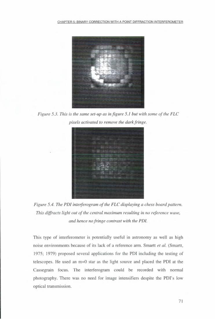
CHAPTER 5: BINARY CORRECTION WITH A POINT DIFFRACTION INTERFEROMETER
mm mm
Figure 5.3. This is the same set-up as in figure 5.1 but with some of the FLC
pixels activated to remove the dark fringe.
Figure 5.4. The PDI interferogram of the FLC displaying a chess board pattern.
This diffracts light out of the central maximum resulting in no reference wave,
and hence no fringe contrast with the PDI.
This type of interferometer is potentially useful in astronomy as well as high
noise environments because of its lack of a reference arm. Smartt et al. (Smartt,
1975; 1979) proposed several applications for the PDI including the testing of
telescopes. He used an m=0 star as the light source and placed the PDI at the
Cassegrain focus. The interferogram could be recorded with normal
photography. There was no need for image intensifiers despite the PDI's low
optical transmission.
71

CHAPTER 5: BINARY CORRECTION WITH A POINT DIFFRACTION INTERFEROMETER
There are several variations of the PDI that are of interest for wavefront sensing
applications. These can be classed as conventional PDIs and phase shifting PDIs.
The conventional PDI can be divided into 4 types:
1. Central field absorption. In this class the transmission function, r(p,9), of the
filter is give by
r(p,e)=i, p>R [5.1]
= a, p < R
where p and 8 are the circular co-ordinates, R is the desired radius of the
central obstruction, and a is the transmission of this obstruction and usually
a=0 in this case. 2. Phase contrast. In this filter the transmission function is
r(p,e) = i, P>R
= e'\ p<R
where <|) is some phase shift between 0 and 271.
3. Field absorption. (Smartt PDI type)
7 = a, p > R
= 1 P<R
4. Field absorption and phase contrast combination
[5.2]
[5.3]
T = a, p > R [5.4]
= e*\ p<R
Anderson (Anderson, 1995) considers all four types of PDI and compares their
fringe visibility, fringe brightness and accuracy. He concludes that the phase
contrast PDI, with cp=7C, performs best when the incident wavefront has a
variance of >(27c)2 and little light loss can be tolerated. However, the field
72

CHAPTER 5: BINARY CORRECTION WITH A POINT DIFFRACTION INTERFEROMETER
absorption PDI has the advantage of been easier to construct and are
commercially available and so this type has been selected.
The wavefront can not be completely calculated with any of the above PDIs.
Phase shifting PDIs have been developed by Kadono et al. (Kadono, 1994) and
Mercer et al. (Mercer, 1996). Both of these systems use nematic liquid crystals
to vary the phase of light passing through the field area of the PDI. Although the
phase can be unwrapped the devices are too slow to be used in astronomical
applications because of the need to take up to 5 interferograms to unwrap the
phase. A modified PDI that diffracts light into three separate interferograms has
been developed (Kwon, 1984) enabling fast unwrapping. It does however need
three detector arrays and is not light efficient, making it unsuitable for
astronomy. Completely unwrapping the phase is not needed in binary adaptive
optics. We are only concerned in finding if part of the wavefront is out of phase
with the rest.
5.3.2 PDI /FLC S Y S T E M CONSIDERATIONS
When the PDI is used in conjunction with the PLC the basic algorithm was:
If a region of the interferogram is dark add K radians phase shift with the
FLC pixel that corresponds to that region.
Several algorithms to determine the threshold value for the intensity have been
considered. The major difficulty is that both the mean intensity and the fringe
contrast change depending on the aberrations. An aberration in the incoming
wavefront will cause the PSF to spread out so less light enters the pinhole. This
reduces the fringe contrast ratio. This light then passes through the
semitransparent aperture, but because this has a lower transmission than the
pinhole the overall intensity of the interferogram drops. We take the familiar
equation for the intensity of two interfering wavefronts of unequal amplitude Ao
and aAo, where a < l ,
73
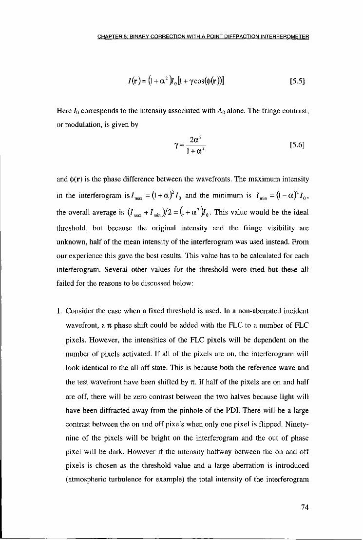
CHAPTER 5: BINARY CORRECTION WITH A POINT DIFFRACTION INTERFEROMETER
/ ( r ) = ( l + a 2 > 0 [ l + Ycos(())(r))] [5.5]
Here /o corresponds to the intensity associated with Ao alone. The fringe contrast,
or modulation, is given by
J = - j [5.6] 1 + or
and <|)(r) is the phase difference between the wavefronts. The maximum intensity
in the interferogram i s / ^ = ( l + a ) 2 / 0 and the minimum is = ( l - a ) 2 / 0 ,
the overall average is (lmax + )/2 = (l + a2 )l0. This value would be the ideal
threshold, but because the original intensity and the fringe visibility are
unknown, half of the mean intensity of the interferogram was used instead. From
our experience this gave the best results. This value has to be calculated for each
interferogram. Several other values for the threshold were tried but these all
failed for the reasons to be discussed below:
1. Consider the case when a fixed threshold is used. In a non-aberrated incident
wavefront, a % phase shift could be added with the FLC to a number of FLC
pixels. However, the intensities of the FLC pixels will be dependent on the
number of pixels activated. If all of the pixels are on, the interferogram will
look identical to the all off state. This is because both the reference wave and
the test wavefront have been shifted by n. If half of the pixels are on and half
are off, there will be zero contrast between the two halves because light wil l
have been diffracted away from the pinhole of the PDI. There will be a large
contrast between the on and off pixels when only one pixel is flipped. Ninety-
nine of the pixels will be bright on the interferogram and the out of phase
pixel will be dark. However i f the intensity halfway between the on and off
pixels is chosen as the threshold value and a large aberration is introduced
(atmospheric turbulence for example) the total intensity of the interferogram
74

CHAPTER 5: BINARY CORRECTION WITH A POINT DIFFRACTION INTERFEROMETER
will be reduced. For certain aberrations the total intensity of the interferogram
will drop below this threshold value and all of the PLC pixels will f l ip
continuously and perform no correction. From experimental observations this
continuous flipping between states happened most of the time.
2. The next value of the threshold to be considered was taking 4Io as the
maximum intensity of the interferogram, I n i a x - This would be the brightest part
of the interferogram and therefore 4/ 0 could be taken to equal 1^ i f a is close
to 1. In this case, the threshold would be Imw/2. This does however not work
in practice because of the non-uniform intensity pattern produced by the PDI.
The interferogram is in fact brighter in the centre and becomes dimmer
towards the edge. This is because the reference wave of the PDI is not from a
point source, but a pinhole, so it does not produce a perfectly spherical wave,
but some other function produced by the diffraction from the pinhole. (This
effect is further compounded by the Gaussian beam profile of the He-Ne laser
source.) This means that the FLC pixels around the edge of the SLM will be
flipped more readily than the ones in the centre. This complication is also
applicable to model 1. In practice the outer pixels of the FLC were
permanently flipped. This introduced aberrations in to the beam. The
assumption that a is close to one also may not hold.
3. Consider taking the threshold as $Imax, where |3 is some real number in the
range 0<p<l. In this case, the above problem of pixels flipping around the
edge of the FLC is reduced by choosing a low value of (3, but this method
does not work when the fringe contrast is low. If this is the case, the mean
intensity, 7 , will tend towards 7 ^ , and so all of the interferogram may be
above the threshold value if a is small and no pixels will be flipped. No value
of a could be found that was low enough to stop the edge FLC pixels flipping
and high enough to work in a low fringe contrast situation.
75

CHAPTER 5: BINARY CORRECTION WITH A POINT DIFFRACTION INTERFEROMETER
4. Consider taking the mean intensity, / , or halfway between the minimum and
maximum, as the threshold (the argument is similar for both). This algorithm
will correct for any dark fringes no matter what the fringe contrast is like. I f
we consider an incident wavefront with a 0 and n phase shift in it, there will
be a dark and light region on the interferogram. The threshold value will be
between the two intensities. The FLC will correct the area that is n out of
phase. The algorithm works in this case. However, i f we now consider a rc/lO
phase shift instead of n in the incident wavefront, we can see that this
algorithm will set the threshold to be between the two intensities again. The
FLC will add TC phase shift to the K/10 region and thus aberrate the beam, so
this algorithm fails.
5. We used half of the mean intensity and so the threshold value is 7/2.
Although this model does not reach a solution in the first frame of correction
in the author's experience this produced the best correction.
To validate this assumption and get a clearer understanding, computer
simulations of the PDI were performed.
5.3.3 COMPUTER SIMULATION
Unlike a Michelson type reference arm interferometer, calculating the
interferogram from the PDI is non-trivial. The total intensity of the interferogram
and the fringe contrast depend upon the incident wavefront. A highly aberrated
wavefront will produce a lower fringe contrast and lower total intensity. In our
system, the correction element is placed in front of the PDI for closed loop
operation and so diffraction effects from the pixels may further complicate
matters.
When the system was run in a feedback loop, the system did not behave as
originally expected. The device did not correct for a given aberration in the first
76
CHAPTER 5: BINARY CORRECTION WITH A POINT DIFFRACTION INTERFEROMETER
frame, but it took several frames to converge towards the best solution. A computer simulation was carried out to gain a better understanding of how the PDI/FLC system was performing the correction.
The simulation was carried out using Mathcad™. A phase aberration was written
to an array, representing the incident wavefront. The data was then fast Fourier
transformed (FFT) to give the amplitude and phase pattern in the PDI plane. An
amplitude aperture mask representing the PDI was then applied to this and the
array was again fast Fourier transformed to give an amplitude pattern in the
interferogram plane. The intensity pattern was calculated from this. From this the
intensity threshold switching value could be calculated. The array was divided
into ten sections to represent the FLC pixels. If the mean pixel intensity was
below the threshold intensity, n radians were added to the initial incident
wavefront and the simulation re-run.
5.3.4 COMPUTER SIMULATION R E S U L T S
Figures 5.5 show the ID simulation results of the correction of 1 wave of
defocus with some global tilt. Figure 5.5 a(i) shows the initial PSF, figure 5.5
a(ii), the simulated PDI interferogram, and figure 5.5 a(iii) the wavefront
incident on the PDI. Figure 5.5 a(iv) shows the reference wave produced by the
pinhole. This is generated by setting the transmission of the opaque screen
surrounding the pinhole to zero. In figures 5.5 b(i-iv) the first correction is made,
in figures 5.5 c(i-iv) the second is made. After the fourth correction (figures 5.5
e(i-iv)) the simulation returns to the same state as that in figures 5.5 d(i-iv). The
simulation oscillates between figures 5.5 e(i-iv) and 5.5 d(i-iv) indefinitely.
The PSFs shown in figures 5.5 a), b), c), and d) (i) are identical to the intensity
pattern focused onto the PDFs aperture. Ideally, in the case of a non-aberrated
incident wavefront, the intensity of the light that has passed through the pinhole
should be equal to the intensity of the light that has passed through the opaque
screen. This gives the best fringe contrast (y=\ in equation [5.5]). When an
77
CHAPTER 5: BINARY CORRECTION WITH A POINT DIFFRACTION INTERFEROMETER
aberrated beam, such as in figure 5.5 a (iii) is incident, the PSF spreads out over
the PDI filter. Because the pinhole and aperture attenuation's are different, the
total amount of light passing through the PDI will be different to the non-
aberrated case. The contrast ratio will decrease because a different amount of
light passes through the pinhole and semi-transparent screen. From these figures
it can be seen that, because of the low fringe contrast in the first frame it is only
possible for the system to perform a partial correction. The reference wave
produced by the PDI is severely attenuated. After the first approximate
correction is made by flipping the correct FLC pixels, the PSF is partially
corrected (figure 5.5 b (i)) and the reference wave is restored (figure 5.5 b (iv)).
This continues until the reference wave and PSF are as fully corrected as
possible.
It can also be seen from figures 5.5 that under certain circumstances oscillations
may occur. This happens when there is an intensity slope on the interferogram
across a region corresponding to an FLC pixel with slightly more than half of the
intensity under the threshold value. This causes the FLC pixel to flip, correcting
the phase of that region and so raising the total intensity of the interferogram,
and hence the threshold value. The intensity slope across the pixel means that the
mean intensity of the pixel is under the new threshold and the FLC flips again
back into its original state, and hence the correction oscillates. This is in
agreement with experimental observations.
78
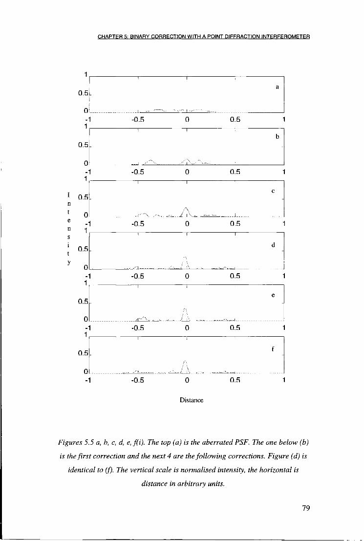
CHAPTER 5: BINARY CORRECTION WITH A POINT DIFFRACTION INTERFEROMETER
Distance
I 0.5. n t 0 e -1 n 1 s i 0.5. t y
0 0
Figures 5.5 a, b, c, d, e, f(i). The top (a) is the aberrated PSF. The one below (b)
is the first correction and the next 4 are the following corrections. Figure (d) is
identical to ( f ) . The vertical scale is normalised intensity, the horizontal is
distance in arbitrary units.
79
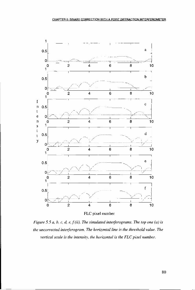
CHAPTER 5: BINARY CORRECTION WITH A POINT DIFFRACTION INTERFEROMETER
1
0.5
0
I n 0.5 t e 0 n 0 s 1 i
I I
c
' V i I I I r
4 6
FLC pixel number
Figure 5.5 a, b, c, d, e,f(ii). The simulated interferograms. The top one (a) is
the uncorrected interferogram. The horizontal line is the threshold value. The
vertical scale is the intensity, the horizontal is the FLC pixel number.
80

CHAPTER 5: BINARY CORRECTION WITH A POINT DIFFRACTION INTERFEROMETER
p 2r h 1 a 0^ s -1 e / 0
w w 1
a 1
V 0 e - 1 ' s
0 0
FLC pixel number
Figure 5.5 a, b, c, d, e, f (iii). The incident phase screens. The vertical scale is in
units of waves. The horizontal scale is the simulated FLC pixel number.
81
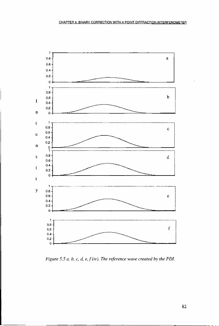
CHAPTER 5: BINARY CORRECTION WITH A POINT DIFFRACTION INTERFEROMETER
1
0.8
0.6
0.4
0.2
0
1
0.8
0.6 I 0.4
n
1 t 0.8
0.6
n o 1
0.8
0.6 0.4
1 0.2
0 t
1
0.8 0.6
0.4 0.2
0
1
0.8 0.6 0.4 0.2
0
Figure 5.5 a, b, c, d, e,f(iv). The reference wave created by the PDI.
82

CHAPTER 5: BINARY CORRECTION WITH A POINT DIFFRACTION INTERFEROMETER
5.4 Experimental FLC/PDI System
5.4.1 SET-UP
Figure 5.6 shows the experimental set-up. The FLC was a 10x10 pixel direct
drive device constructed by Displaytech with 0.885mm x 0.885mm pixels and
0.115mm inter-pixel spacing. The device was controlled by an 80486 PC with a
Texas Instrument's C40 parallel processor mounted on a Coreco F/64-DSP
frame grabber.
Laser B E
L I L2 POL BS L3 LA
Abemtion F L C PDI CCD 1
CCD 2
Figure 5.6. The experimental set up. L1-L5 lenses, BS beam splitter, POL
polariser, BE beam expander and spatial filter, FLC ferroelectric liquid crystal
SLM, PDI point diffraction interferometer. The aberration was generated with a
Meadowlark Hex69.
A collimated lOmW polarised He-Ne laser was used for illumination. A
polariser was placed after the FLC. A beam splitter was used to split half of the
light to the science camera (CCD2) which measures the PSF of the system. A
lens focuses the other half onto the PDI's aperture. Doublet lenses where used
throughout the system to minimise spherical aberrations.
Aberrations were introduced into the system by placing the Meadowlark Hex69
nematic liquid crystal SLM in front of the FLC SLM.
83

CHAPTER 5: BINARY CORRECTION WITH A POINT DIFFRACTION INTERFEROMETER
5.4.2 CONTROL HARDWARE
A Coreco F/64-DSP board was used for the image processing. Its specifications
are shown in table 5.1
Specification Value
Video memory (VRAM) 2Mbytes
Digitisation accuracy 8 bit
Dynamic Memory (DRAM) 1 Mbyte
Camera * Standard CCIR
Frame rate * 25 Hz
Frame size * 768 x 575 (8-bit)
Image processor TMS320C40
Display VGA monitor
Table 5.1. The image acquisition equipment and processor. The frame board
was capable of interfacing with many different types of CCD camera, values
indicated by * are user settings and depend on the type of camera.
The PC was an 80486 DX2 66MHz with 16Mbytes of RAM. See figure 5.7 for
the systems design.
F/64 DSP
HOST PC
CCD
Monitor
SLM
Figure 5.7. The image processing and control hardware system.
84
CHAPTER 5: BINARY CORRECTION WITH A POINT DIFFRACTION INTERFEROMETER
5.4.3 CONTROL SOFTWARE
Two programs were required to control the system: one for the DSP and one for
the PC. The DSP software was loaded from the PC's MS-DOS command line
and could only be executed by a function call from the PC software. The image
processing was performed on the C40. Its results were passed to the PC over the
computer's ISA bus. The C40 has direct access to the frame grabber's video
RAM area over the F/64's high speed 32 bit internal bus. Because the image is
stored in 8 bits, it was necessary for four pixel values to be read every time only
one is required. This 32 bit word had to be separated into four 8 bit words to get
the required pixel value. This process took up a considerable amount of C40
processor time because several functions had to be called and there were a large
number of pixels on the camera to be processed.
The system was aligned by writing 100 10x10-pixel squares to the video
monitor. At the same time, the CCD1 camera was acquiring the image of the
interferogram and the PLC was slowly flipping each single pixel consecutively.
The CCD camera was moved until the squares drawn on the screen were
perfectly aligned with the FLC pixels.
Once the FLC and camera were aligned, the correction routine could be run. The
alignment squares were no longer drawn because of the slowness of the routine.
The PC software then called the DSP routine. The mean intensity was calculated
by the C40 of each of the regions corresponding to the FLC pixels. This data was
stored in a one hundred element array and this array was passed to the PC over
the ISA bus. The PC then calculated the mean intensity and used half of this
value as the threshold. The threshold value was then compared to the mean
intensity of each FLC pixel area and a 10 by 10 one bit array was generated
corresponding to which pixels should be flipped. This array had then to be
exclusively ORed (XOR) bitwise with the previous screen to calculate the array
to send to the FLC. To see why we XOR the data with the previous screen
85

CHAPTER 5: BINARY CORRECTION WITH A POINT DIFFRACTION INTERFEROMETER
consider just one FLC pixel. Initially the FLC pixel is set to zero. I f the interferogram region corresponding to that FLC pixel becomes darker then the threshold value the FLC pixel wil l be flipped. However, in the next frame this pixel must not be turned off just because interferogram is now above the threshold. It must be left on until the interferogram area of the pixel becomes darker than the threshold again. Table 5.2 contains the logic table of the XOR function.
p D R
0 1 1
1 0 1
1 1 0
0 0 0
Table 5.2. P represents the previous pixel value; D is the current thresholded
result from the interferogram and equals 1 for a dark pixel and Ofor a light
pixel. P XOR D gives R which was then applied to the FLC array. In the next
frame P will be set equal to R.
86

CHAPTER 5; BINARY CORRECTION WITH A POINT DIFFRACTION INTERFEROMETER
START
* Align system?
NO
f Calculate threshold
I Threshold pixels
J Write to FLC
PC
YFS
"** Grab image
Draw alignment marks
i
.Grab image and calculate pixel
intensities
DSP
Figure 5.8. The flow chart of the control software for the FLC/PDI system. The
PC and DSP sections are linked via the ISA bus.
Once the correct array was calculated it was sent to the PC's printer port which
was connected to the FLC drive electronics. The next frame of the CCD camera
was then taken and the process repeated (see figure 5.8).
5.4.4 C O R R E C T I O N R E S U L T S
Figures 5.9 show the resultant PSFs taken with CCD2. Figure 5.9 a) shows the
unaberrated PSF. The Strehl ratio is taken as 100% of the maximum intensity of
the unaberrated PSF. Figure 5.9 b) shows the PSF with an aberration introduced
into the system. The aberration was a defocus Zernike function with a peak to
valley amplitude of 0.44A. (632.8 nm) and gave a Strehl ratio of 5%. Figure 5.9
c) shows a typical corrected PSF. Figure 5.10 shows the actual images of the
87

C H A P T E R 5: B I N A R Y C O R R E C T I O N WITH A P O I N T D I F F R A C T I O N I N T E R F E R O M E T E R
PSFs. The corrected Strehl ratio was 26%, a five-fold increase. When the aberration was removed, the system returned to its initial state (i.e., the FLC pixels turned off and the Strehl ratio returned to 100%).
1
0.8
0.6
0.4
0.2
0 100
100 50
50
0 0
Figure 5.9 (a). The unaberrated PSF. The Strehl ratio is defined as being 100%
at the peak intensity.
88

C H A P T E R 5: B I N A R Y C O R R E C T I O N WITH A P O I N T D I F F R A C T I O N I N T E R F E R O M E T E R
1
0.8
0.6
0.4
0.2
0 100
00 50
50
0 0
Figure 5.9(b). The aberrated PSF. The Strehl ratio was 5%.
89
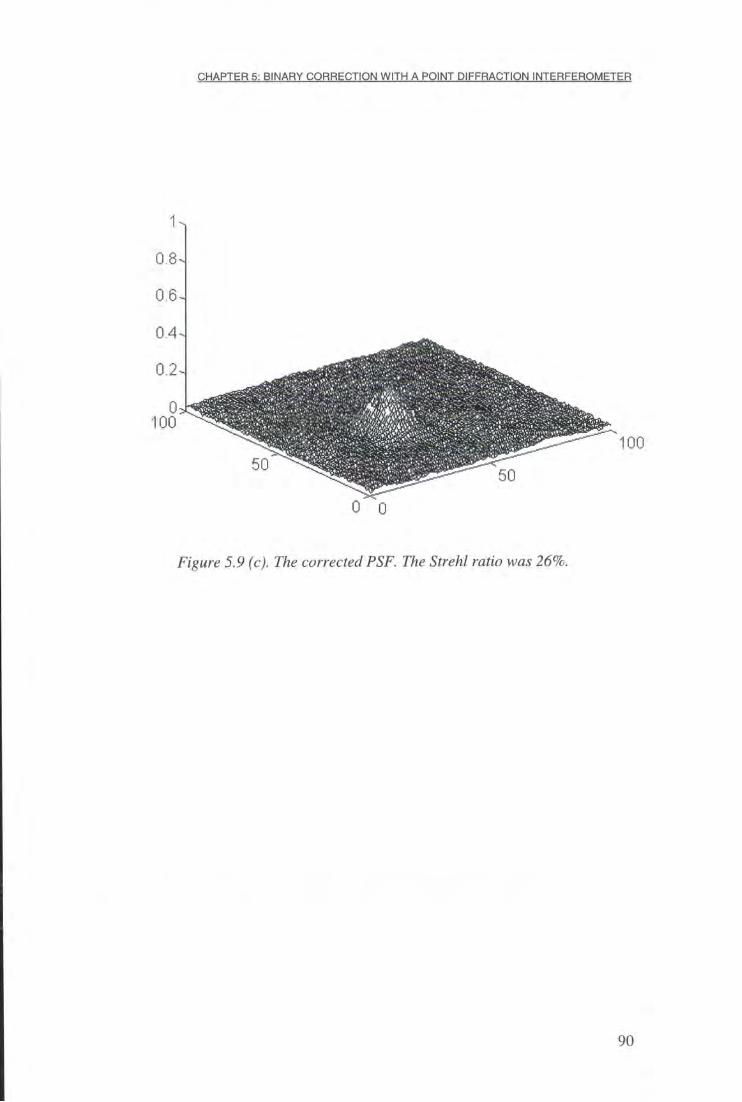
C H A P T E R 5: B INARY C O R R E C T I O N WITH A P O I N T D I F F R A C T I O N I N T E R F E R O M E T E R
1 0.8
0.6
0.4
0.2
0 00
00 50
50
0 0
Figure 5.9 (c). The corrected PSF. The Strehl ratio was 26°7t
90
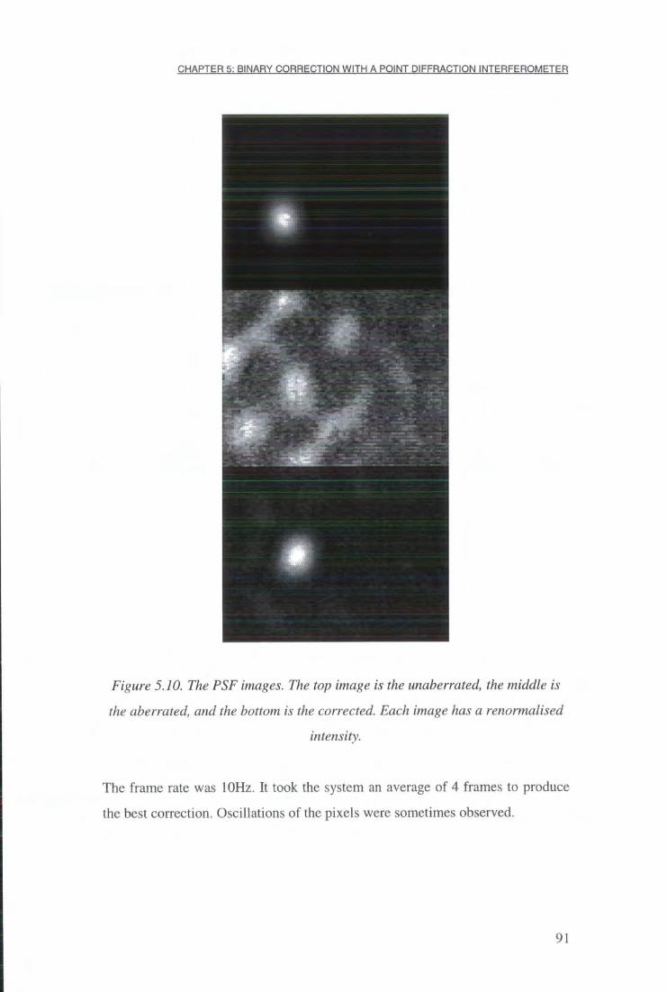
C H A P T E R 5: B I N A R Y C O R R E C T I O N W I T H A P O I N T D I F F R A C T I O N I N T E R F E R O M E T E R
Figure 5.10. The PSF images. The top image is the unaberrated, the middle is
the aberrated, and the bottom is the corrected. Each image has a renormalised
intensity.
The frame rate was 10Hz. It took the system an average of 4 frames to produce
the best correction. Oscillations of the pixels were sometimes observed.
91

C H A P T E R 5: B I N A R Y C O R R E C T I O N W I T H A P O I N T D I F F R A C T I O N I N T E R F E R O M E T E R
5.4.5 F L C OPTICAL THROUGHPUT
The optical throughput of the FLC was measured using a non-polarised laser.
The intensity was measured with a CCD camera. The transmission of the F L C
with no polarisers was (78±4)%. The throughput of a single polariser was
(32±2)% and the throughput of the F L C with the two polarisers in place was
(2±0.5)%. This compares reasonably with the calculated transmission above if
the transmissions of each component are taken into account. From [2.10] the
theoretical transmission is 33%, correcting this with the optical transmission of
each component, the total transmission is reduced to 2.6%. It should be noted
that the polarisers used to calculate the throughput were of lower quality than the
polariser in the main experiment which had a quoted transmission of 42%.
5.5 Discussion
With the system in a closed loop, it was not possible to stop FLC pixel
oscillations with our simple algorithm. However, the system still produces a
five-fold improvement in the Strehl ratio. One way round the oscillations would
be to run the device in an open loop system. In this configuration, the F L C
would not be in the same optical arm as the PDI but in front of the science
camera (see figure 5.6). Since our system has to work towards the best solution it
is not known how well the FLC SLM would perform in open loop. It would also
not correct any systematic errors such as optical non-uniformities in the F L C
SLM.
Despite the low number of pixels (100) the F L C device has still managed to
partially correct for an aberration that is typically associated with a telescope of
size 12ro -1-2 metres (Wang, 1978), where r 0 is the Fried parameter (typically
10-20cm). Love et al. (Love, 1995) have shown that a 128x128 pixel device
would be capable of correcting atmospheric aberrations across a telescope of up
to 40 ro in diameter. Such devices are currently available commercially, although
their suitability has not been fully investigated.
92
C H A P T E R 5: B I N A R Y C O R R E C T I O N W I T H A P O I N T D I F F R A C T I O N I N T E R F E R O M E T E R
The corrected Strehl ratio of 26% is somewhat lower than the quoted theoretical limit of 40.5%. This is to be expected because of the large residual wavefront errors caused by the finite size, and the finite number of F L C SLM pixels.
A major limitation of the FLC SLM used in this experiment was that its
retardance was neither n nor was its switching angle 90°. This would be needed
if such a device were to be used for light starved astronomical purposes where a
high transmission is required. The retardance of our system was 0.6K and it had a
switching angle of 45° giving a maximum theoretical transmission of 33%, and
an experimentally measure transmission of 2% (including polarisers). Although
no company to date has produced a high switching angle FLC SLM, it should be
easier to control the retardance of future devices by fine tuning the cell thickness.
If a device with n retardance could be produced, the theoretical transmission
would be improved to 50% even with a switching angle of only 45°.
Tip/tilt has not been corrected in this experiment. The PDI could not measure
large amounts of tip/tilt since the focused beam moved away from the aperture in
the centre of the PDI mask. Tip/tilt would need to be removed with a mirror
before the light was corrected by the FLC. This would require an additional
sensor (such as a quad cell) and so the light throughput of the total system would
be further reduced.
5.5.1 PHOTON F L U X
Liquid crystal devices offer the possibility of a very large number of pixels.
Monitors in laptop computers have typically 640x480 pixels, although their low
pixel fill factor and low optical flatness makes them unsuitable for astronomical
adaptive optics. Displaytech currently offer a 256x256 device with a high fill
factor (87%) and a frame rate of 3kHz (Ref. Displaytech). This gives a much
greater number of degrees of freedom than a standard deformable mirror.
93

C H A P T E R 5: B I N A R Y C O R R E C T I O N W I T H A P O I N T D I F F R A C T I O N I N T E R F E R O M E T E R
Increasing the number of pixels to a much larger extent will, however, slow
down the operating speed of the system. Computation time aside, the number of
photons from an astronomical source is limited and fixed. If the number of
pixels is doubled the integration time required is also doubled. The number of
photons detected per FLC pixel, Ndet, in integration time, T, is given by
Q-Nl T\ - F x
where n is the number of pixels, Q is the quantum efficiency of the detector, M
is the incident number of photons into the interferometer, r\ is the efficiency of
the PDI, and F is the fill factor of the device. Nj is (Schroeder, 1987)
Nj = N • D2 • AX - 10~° 4 me [5.8]
where N=108 is the number of photons per second per metre squared per
nanometre for a zeroth order AO star at 550nm, AX, is the bandwidth and is
40nm, m is the stellar magnitude, and £=50% is the efficiency of the system to
the front end of the interferometer. For a lm telescope, imaging a magnitude 7.7
star, Nj is approximately 1.6xl06 photons per second. The value of T | depends on
the incident wavefront and is typically as low as 5% (Love, 1995). Assuming a
quantum efficiency of 0.8, F=100%, and n=100; A^£/=0.166 photons per frame
per pixel at the maximum frame rate of 4000Hz. Clearly, the device could not be
operated at such speed. If we limit the frame rate to that required to correct for
typical atmospheric aberrations, about 100Hz, we find for at least one photon per
frame per pixel the maximum number of pixels is 665 or about 25x25. This
assumes that the transmission of the FLC is 100%. If the current Displaytech
device is used, the transmission becomes substantially worse. With only 2%
transmission, the maximum number of FLC pixels for one photon per frame is
only 13 (or -3x3).
94

C H A P T E R 5: B I N A R Y C O R R E C T I O N W I T H A P O I N T D I F F R A C T I O N I N T E R F E R O M E T E R
Because the number of photons entering the telescope is proportional to the diameter of the telescope squared, we can rearrange equation [5.7] to calculate the maximum number of F I X SLM pixels usable in a telescope of diameter D
n<Q - Nj l m e l r e r\ - F • D2 • t [5.9]
12000 -|
10000 in
8000
LL 6000
S 4000
2000
i
1 1.5 Telescope diameter / metres
Figure 5.11. The maximum number of pixels that could be used in a telescope
versus the diameter of the telescope. The solid line is for r)=5%, the dotted line
is for 7]= 100%.
Ni i metre is the photon flux for a 1 metre telescope. If i = 10ms, the number of
pixels versus telescope diameter is shown in figure 5.11 for both T)=5% and
r|=100%. It is important to maximise the number of PLC SLM pixels in order to
reduce the residual wavefront error after correction in order to get as close as
possible to the maximum corrected Strehl ratio of 40.5%.
To improve the photon flux the most obvious solution is to increase r\. It should
be noted that TJ depends on the aberration. For a well corrected aberration r| will
increase. If the PDI was replaced by a phase contrast PDI the value of r\ would
increase to -100%, increasing the number of photons 20 fold.
95
C H A P T E R 5: B I N A R Y C O R R E C T I O N WITH A P O I N T D I F F R A C T I O N I N T E R F E R O M E T E R
The above calculation does not take into account the absorption of the optical
components in the telescope and any real system would require more than one
photon to operate. It does show that to run a pixelated adaptive optics system in
a telescope it is necessary to carefully balance the number of pixels with the
available light.
The system could be tested on a telescope system providing the following
criteria can be achieved:
• An FLC with 0-K phase shift can be developed with a high transmission.
• The speed of the system can be increased.
• The transmission of the PDI can be increased.
5.5.2 F U T U R E CONSIDERATIONS
The system is currently limited to 10Hz. This is because of the large amount of
image data from CCD 1 (figure 5.6) that has to be processed by the C40
processor chip (768 x 575 bytes of data per frame). If a higher speed camera,
such as the DALSA used in chapter 7 replaced the CCD camera used, the system
bandwidth should be improved. This camera has a maximum frame rate of
838Hz and 128x128 pixels. It should be possible to operate this system at speeds
in excess of 100Hz, which would be adequate for most astronomical
applications. This does not however take into account the efficiency of the
camera, which is quite low, but other similar cameras are available with higher
efficiencies.
Because the system takes more than one frame to reach the optimum solution,
the system will have to be operated several times faster than an aberration. The
precise speed needed is yet to be determined. The system took four frames to
reach the optimum correction in §5.4. However, it did partially correct in the
96

C H A P T E R 5: B I N A R Y C O R R E C T I O N WITH A P O I N T D I F F R A C T I O N I N T E R F E R O M E T E R
first frame. It is unclear how the system will operate in a time evolving situation.
It is possible that once the system has achieved the correction, any small
perturbations made to the aberration will be corrected in the next frame.
If a larger FLC SLMs were to be used in the future this would again slow down
the system because of the large amount of data. The Coreco F/46 board used in
this experiment has the capabilities of mounting more C40 chips and so
increasing its computing power. A cheaper alternative would be to use an array
of photodiodes instead of a CCD camera to image the interferogram. The
position of each photodiode would correspond to each F L C pixel. If each
photodiode was connected to a simple thresholding circuit, the whole system
could be built to work at the maximum speed of the FLC SLM (4000Hz). In
reality, for astronomical purposes the limit would be the number of photons
entering the telescope needed to trigger the photodiodes.
5.6 Summary
In this chapter a binary adaptive optics system has been demonstrated using a
PDI and 10x10 FLC SLM. The technique does not attempt to fully correct an
aberrated wavefront but still an improvement in Strehl ratio from 5% to 26%
was achieved. The frame speed of the system was 10Hz and this is currently
limited by the computer power. A model of the PDI was also developed with a
suitable threshold value.
The potential for an F L C SLM with a Shack-Hartmann wavefront sensor is
discussed in the next chapter. This wavefront sensor is commonly used for
adaptive optics and does not have many of the problems that have been found
with the PDI such as the low through-put or the oscillations caused by the PDI's
unusual characteristics.
97
CHAPTER 6: A LIQUID CRYSTAL ATMOSPHERIC T U R B U L E N C E SIMULATOR
Chapter 6: A Liquid Crystal Atmospheric
Turbulence Simulator
6.1 Introduction
There is a need to test all adaptive optics systems by introducing aberrations into
the optical beam. This can be achieved in one of three ways: try the system on a
telescope; use a deformable mirror to introduce known aberrations; or introduce
unknown aberrations such as turbulence generated by a heating element, a fan or
a rotating piece of aberrated glass. The first option is naturally the best for an
astronomical adaptive optics system, but it requires shipping the device to a
telescope and allocating telescope time which can be difficult and expensive.
The use of deformable mirrors is very expensive. The third option uses non-ideal
statistics and is not very controllable. In this chapter we develop a liquid crystal
based atmospheric turbulence simulator (ATS). This will be used to generate
aberrations with scaleable Kolmogorov statistics for testing the adaptive optics
system in chapter 7. It will also be of potential use to the whole of the adaptive
optics community.
6.2 Background
Previous adaptive optics systems using liquid crystals have only concentrated on
static correction. To introduce an aberration into a system such as this is trivial: a
piece of non-flat glass can be inserted into the optics, or even the aberration
introduced by the SLM itself when the SLM is of low optical quality.
When an adaptive optics system is to work in real time the situation becomes
more difficult. A method of producing variable aberrations of the correct
amplitude, phase, and speed is required. A mechanical system could be
constructed such as a piece of aberrated glass rotated with an electrical motor.
Although simple this technique would have several problems. The aberrations
would be cyclic, i.e., they would be repeated after the glass has rotated 360°. The
98

CHAPTER 6: A LIQUID CRYSTAL ATMOSPHERIC TURBULENCE SIMULATOR
motor could introduce large amounts of tip/tilt from mechanical vibrations; a
problem for liquid crystal correction where tip/tilt stroke is limited. It also will
not have the correct power spectrum of the desired aberration to be modelled
unless the glass is specifically made that way.
A device that could be used to generate a time varying aberration with the
correct statistics would clearly be useful for testing the performance of an
adaptive optics system. The statistics to be used in the case of atmospheric
turbulence are Kolmogorov. To the author's knowledge there has been little
work on producing simulated turbulence. Most groups use either heater/fan type
arrangements or expensive deformable mirrors. A second deformable mirror
only used for laboratory simulation is prohibitively expensive. This chapter
presents an alternative method using liquid crystal SLMs.
6.3 Requirements for an Atmospheric Turbulence
Simulator (ATS)
Any ATS must fulfil the following criteria:
1. It obeys Kolmogorov statistics.
2. It needs to be relatively small. The whole point is that it fits on the optical
bench.
3. It should be able to simulate various wind speeds.
4. It should be able to simulate various values of D/ro.
5. It should not be cyclic, i.e., the phase screens should not repeat for at least a
reasonably long time.
6. It needs to produce the correct Strehl ratio and PSF.
7. The aberrations should be continuous and have no sharp discontinuities.
Points 3 and 4 are so that different sized telescope diameters and wind speeds
can be modelled.
99

CHAPTER 6: A LIQUID CRYSTAL ATMOSPHERIC TURBULENCE SIMULATOR
6.4 A Liquid Crystal SLM as an ATS
Of the two possible liquid crystal materials that could be used for an ATS, only a
nematic device is really suitable. An FLC is considerably faster but will only
introduce 0/n aberrations into a wavefront. This will not fully test any system
that provides analogue correction. Nor will it introduce aberrations with the
correct statistics. It was shown in chapter 4 that the multiplexed 64x64 SLM will
not produce the correct phase pattern. For this reason a Meadowlark Hex69
nematic liquid crystal SLM was used. This device is now an 'off the shelf
package, but it was originally designed for the University of Durham's adaptive
optics program.
The concept behind the Hex69 design was for correcting aberrations. Therefore,
in principle, it should be equally as good at generating aberrations. It is a nematic
device and capable of giving an analogue response. Love (1997) has shown the
device does introduce Zernike aberrations into collimated beams well (~A/10
error), but he did not assess the performance with either a real time aberration, or
more than one mode. The following sections will attempt to do that. The basic
principle behind the ATS is to generate simulated phase screens off-line and then
map them onto the SLM in real time.
6.5 Meadowlark Hex69 Device Description
The pixels are in a hexagonal format which is shown in figure 6.1. This format
allows either a circular aperture or a square aperture. There is total of 69 pixels;
each is directly driven, i.e., there is an individual electrode to each pixel. The
liquid crystal material is sandwiched between two layers of optically flat quartz
with the indium tin oxide (ITO) electrodes deposited and then the pattern
lithographically etched on the inside surface. The liquid crystal was controlled
by an AC electric field that could be varied from 0 to 10V in divisions of lmV.
The potential across each pixel was controlled by a PC. The specifications are
given in table 6.1.
100
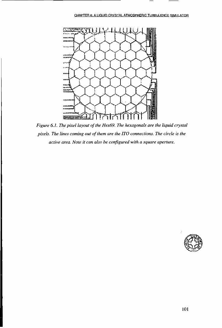
CHAPTER 6: A LIQUID C R Y S T A L ATMOSPHERIC TURBULENCE SIMULATOR
c
1 J I T y ^ s . > *"S . r r i
T I
Figure 6.1. The pixel layout of the Hex69. The hexagonals are the liquid crystal
pixels. The lines coming out of them are the TTO connections. The circle is the
active area. Note it can also be configured with a square aperture.
101
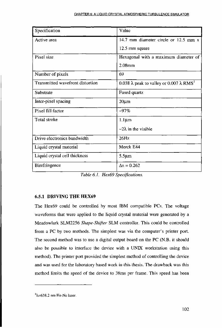
CHAPTER 6: A LIQUID CRYSTAL ATMOSPHERIC TURBULENCE SIMULATOR
Specification Value
Active area 14.7 mm diameter circle or 12.5 mm x
12.5 mm square
Pixel size Hexagonal with a maximum diameter of
2.08mm
Number of pixels 69
Transmitted wavefront distortion 0.038 X peak to valley or 0.007 X RMS 1
Substrate Fused quartz
Inter-pixel spacing 20Lim
Pixel fill factor -97%
Total stroke l.lLtm
~2X in the visible
Drive electronics bandwidth 26Hz
Liquid crystal material Merck E44
Liquid crystal cell thickness 5.5|im
Birefringence An = 0.262
Table 6.1. Hex69 Specifications.
6.5.1 DRIVING T H E HEX69
The Hex69 could be controlled by most IBM compatible PCs. The voltage
waveforms that were applied to the liquid crystal material were generated by a
Meadowlark SLM2256 Shape-Shifter SLM controller. This could be controlled
from a PC by two methods. The simplest was via the computer's printer port.
The second method was to use a digital output board on the PC (N.B. it should
also be possible to interface the device with a UNIX workstation using this
method). The printer port provided the simplest method of controlling the device
and was used for the laboratory based work in this thesis. The drawback was this
method limits the speed of the device to 38ms per frame. This speed has been
'^=638.2 nm He-Ne laser.
102
CHAPTER 6: A LIQUID C R Y S T A L ATMOSPHERIC TURBULENCE SIMULATOR
measured using a 33MHz 80386 and a 66MHz 80486 PC and appears to be
machine independent. Using a digital output board would enable the device to be
run at higher speeds, however the speed of the liquid crystal would not increase
so an improvement in speed would only be noticed for small differences in the
phase shift between each frame.
6.6 The Hex69 as an ATS
6.6.1 PHASE S C R E E N GENERATION METHODS
There are currently several methods of generating atmospheric phase screens.
Roddier (Roddier, 1990) used a method involving Zernike modes. Although the
major advantage of this was the high calculation speed of each mode and the fact
that it produced a circular phase screen that would map onto the Hex69 well. It
was necessary to produce 400 Zernike modes to obtain an accurate
representation of the atmosphere. It is also unresolved how to generate a time
varying phase screen with this method.
6.6.2 LANE'S F O U R I E R METHOD
Lane and Glindemann (Lane, 1992) (Glindemann, 1993) produced phase screens
using a Fourier convolution method. The basic technique can be summarised as
follows. A square array is filled with random numbers. The array is then scaled
by the power spectrum of the Kolmogorov turbulence. This is then fast Fourier
transformed (FFT) into real space to produce the simulated phase screen. To
achieve the correct statistics for the lower order modes a very large amount of
data needs to be modelled (>several times the telescope diameter). To reduce the
need for such large amounts of data to be calculated, lower order Zernike modes
are added in instead. This technique can be used to generate time evolving phase
screens. By generating a large rectangular array, an aperture can be moved across
the array to give the effect of temporal variation.
103

C H A P T E R 6: A LIQUID C R Y S T A L A T M O S P H E R I C T U R B U L E N C E S I M U L A T O R
6.6.3 SOFTWARE
Software written in FORTRAN 77 was provided by Glindemann to calculate the
phase screens. The data was generated on a SUN SPARC STATION IPC. Two
thousand frames were generated, taking several hours. To avoid aliasing, the
data arrays were twice as big as the telescope diameter. Each frame was a
128x128 floating point array, requiring a total of 125Mb of disk space. The data
parameters used to generate the screens are shown in table 6.2.
Parameter Value
D/r0 1
Total array size 128x128 4 byte floating point
Size of aperture data 64x64 4 byte floating point
Number of elements moved per 2
frame2
Number of lower order modes added 7
Total number of frames 2000
Table 6.2. The specifications for the atmospheric turbulence screens to be
generated.
A value of D/r0= 1 was chosen so that the raw phase could be scaled by a factor
of (D/r0)5B to simulate any telescope diameter. The wind speed is related to D,
the number of elements moved per frame Nm, the number of elements in the
array Ne and the frame speed of the SLM, F. The wind velocity, v*, is the
distance travel per frame divided by the frame speed. So
>.=%D 1 [6.1]
_ _2_ 1 ~ 6 4 ' '38-10 - 3
2I.e., the frame is shunted to the left of the previous frame by two element/pixels.
104
C H A P T E R 6: A L IQUID C R Y S T A L A T M O S P H E R I C T U R B U L E N C E S I M U L A T O R
= 0.822 ms"1
or about 3km h r " f o r a lm telescope. This is a very still day but it can be
increased by increasing the value of Nm up to maximum of 64, giving vx= 95km
hr"1, although at the expense of the correlation between consecutive frames.
The liquid crystal in the Hex69 SLM is too slow to accurately produce the large
phase shifts required by the tip/tilt terms when the SLM is running at ful l speed.
It has been assumed that a real liquid crystal adaptive optics system would have
a separate tip/tilt mirror, for this reason tip/tilt was not modelled. The generated
data was separated into individual files and the tip/tilt and piston was removed
by a least squares fitting program. The mean phase over each of the Hex69
pixels was then calculated and this was written to a file containing the 69x2000
pixel values.
The software supplied with the Hex69 could only handle a maximum of 96
frames. This would only give 3-4 seconds of turbulence. To use all 2000 frames
generated new software was developed by the author. This was written in C and
compiled with a Semantec C++ compiler. This compiler has a 32-bit DOS
extender option, and unlike ordinary compilers it allows full access the PC's
RAM instead of the usual 640kb limit imposed by MS-DOS.
The program had several command line options: the number of frames skipped,
A; the frame speed, v, the scale, a; and the data file name. The data file was read
into an array and scaled by the amount a. A was to make the wind speed
variable, changing it to be more than unity reduced the total number of frames
available but it was more convenient than regenerating all of the data from
scratch. The frame speed was limited to a minimum of 38ms.
The data was converted into voltages by the polynomial measured in §6.7.3.
Once the data was in the correct format it was sent to the SLM via the
105

C H A P T E R 6: A L IQUID C R Y S T A L A T M O S P H E R I C T U R B U L E N C E S I M U L A T O R
computer's printer port. Using this method the only limit on the number of
screens that can be used was the amount of RAM of the PC. The ATS took 76
seconds to completely run through all 2000 frames. Once the end of the data was
reached, the data was run through backwards so that there was no sharp
discontinuity between frame 2000 and frame 1.
Zernike modes could also be applied to the device using pre-existing software
modified for this device by the author. The software calculated the phase over
each pixel by using the Zernike modes of table 3.2. The phase was then
converted to voltages using the calibration polynomial.
6.7 ATS Performance Measurements
To characterise the performance of the Hex69 as an ATS, both the spatial and
temporal characteristics of the system need to be measured. This performance
was measured in three ways: the temporal power spectrum of the phase, the
Zernike power spectrum and the Strehl ratio. Ideally, the measurements should
be taken over as many phase screens as possible. To measure the power
spectrums a Shack-Hartmann wavefront sensor was used.
6.7.1 T H E SHACK-HARTMANN WAVEFRONT SENSOR
A Shack-Hartmann wavefront sensor measures Zernike modes in the incident
wavefront. Because it can completely determine the wavefront (except for the
piston term) in real time and from one measurement, it is ideal for measuring the
performance of an ATS. The Shack-Hartmann is also used in many adaptive
optics systems and will be the wavefront sensor for the systems described in the
next two chapters.
The interaction matrix, B, (equation [3.28]) was calculated off line by
calculating the differential for each mode in each axis for all of the theoretical
spot centres. The actual values of the elements of B depend upon the size and
106

C H A P T E R 6: A L IQUID C R Y S T A L A T M O S P H E R I C T U R B U L E N C E S I M U L A T O R
shape of the lenslet array. Then the pseudoinverse of B was calculated off line. These calculations were done with MATLAB™.
6.7.2 HARDWARE AND OPTICAL SET-UP
The computer hardware set-up was similar to that described in chapter 5. A C40
processor was mounted on a frame grabber and hosted in a 486 PC, the set-up is
shown in figure 5.7. The camera used for the Shack-Hartmann was a DALSA
CA-D1-0128 with a data rate of 16MHz. The camera had 128x128 pixels and a
frame rate of 838Hz. The pixels were arranged in a square array,
2.048x2.048mm in size. This camera was not optimised for low light
environments, however since a laser was the source there was no shortage of
photons.
I
Laser L I M LA CCD1
Figure 6.2. The optical set-up of the Shack-Hartmann/Hex69 system. LI, L2, L3
are doublet lenses, LA is the lenslet array, M is the Hex69 SLM, and CCD1 is
the DALSA CCD camera. The laser is spatially filtered, beam expanded and
then re-collimated by LI.
107

C H A P T E R 6: A L IQUID C R Y S T A L A T M O S P H E R I C T U R B U L E N C E S I M U L A T O R
Figure 6.3. The approximate sampling of the Hex69 pixels (thin lines) by a
Shack-Hartmann lenslet (dark line).
The optical set-up is shown in figure 6.2. A lOmW He-Ne laser was the light
source. This was collimated and beam expanded to ~2cm diameter. The two
lenses L2 and L3 demagnify the beam so that at least 3 Hex69 pixels are
sampled by a lenslet (see figure 6.3). If there were only 2 pixels sampled by the
Shack-Hartmann it could have only measured tilt in one direction. If there were
only one pixel there would be no measurement because only the piston of the
phase would change. 19 lenslets are used to sample the wavefront. The image of
the spots for an unaberrated beam is shown in figure 6.4. Figure 6.5 shows the
same spots with 0.5A. of defocus added by the Hex69.
108
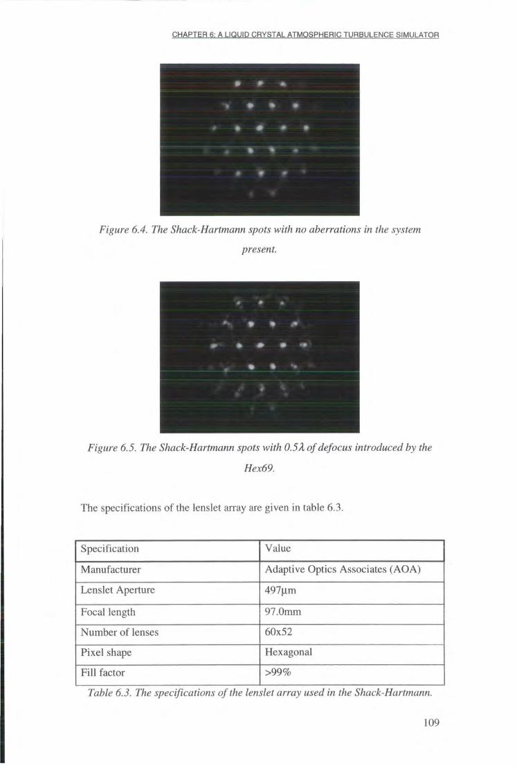
C H A P T E R 6: A LIQUID C R Y S T A L A T M O S P H E R I C T U R B U L E N C E S I M U L A T O R
» W *
* • | • * * • • •
% % *
Figure 6.4. The Shack-Hartmann spots with no aberrations in the system
present.
* # *
* *• * • • «•
» % • *•
w
Figure 6.5. The Shack-Hartmann spots with 0.5A of defocus introduced by the
Hex69.
The specifications of the lenslet array are given in table 6.3.
Specification Value
Manufacturer Adaptive Optics Associates (AOA)
Lenslet Aperture 497u.m
Focal length 97.0mm
Number of lenses 60x52
Pixel shape Hexagonal
Fill factor >99%
Table 6.3. The specifications of the lenslet array used in the Shack-Hartmann.
109
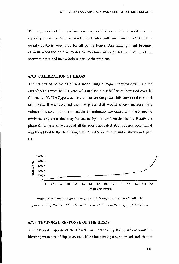
C H A P T E R 6: A L IQUID C R Y S T A L A T M O S P H E R I C T U R B U L E N C E S I M U L A T O R
The alignment of the system was very critical since the Shack-Hartmann typically measured Zernike mode amplitudes with an error of A/100. High quality doublets were used for all of the lenses. Any misalignment becomes obvious when the Zernike modes are measured although several features of the software described below help minimise the problem.
6.7.3 CALIBRATION OF HEX69
The calibration of the SLM was made using a Zygo interferometer. Half the
Hex69 pixels were held at zero volts and the other half were increased over 10
frames by IV. The Zygo was used to measure the phase shift between the on and
off pixels. It was assumed that the phase shift would always increase with
voltage, this assumption removed the 2% ambiguity associated with the Zygo. To
minimise any error that may be caused by non-uniformities in the Hex69 the
phase shifts were an average of all the pixels activated. A 6th degree polynomial
was then fitted to the data using a FORTRAN 77 routine and is shown in figure
6.6.
10000 -i
> 8000-E
6000 • o> 3 4000 -o > 2000 •
0-0 0.1 0.2 0.3 0.4 0.5 0.6 0.7 0.8 0.9 1 1.1 1.2 1.3 1.4
Phase shift /lambda
Figure 6.6. The voltage versus phase shift response of the Hex69. The
polynomial fitted is a 6th order with a correlation coefficient, r, of0.998776
6.1.4 T E M P O R A L RESPONSE OF T H E HEX69
The temporal response of the Hex69 was measured by taking into account the
birefringent nature of liquid crystals. I f the incident light is polarised such that its
110

C H A P T E R 6: A L IQUID C R Y S T A L A T M O S P H E R I C T U R B U L E N C E S I M U L A T O R
axis of polarisation bisects the ordinary and extraordinary axis of the liquid
crystal, the SLM will modulate intensity instead of phase. The usual phase shift
A then appears as a modulation term and the intensity is
I = IQsm2(y2) [6.2]
From figure 6.6, the value of A moves through about 1.5 wavelengths, i.e.,
through about 3n radians. Whenever A is an odd multiple of n the intensity is
maximised, whenever it is an even number of n the intensity is zero. This can be
seen in figure 6.7.
A photodiode was connected to a digital storage oscilloscope (DSO) to measure
the temporal response. The SLM pixels were modulated between two voltages at
the maximum speed. These voltages corresponded to a known phase shift
calculated from the calibration curve. The response times are shown in table 6.4.
The rise time of the liquid crystal was approximately the same for all applied
voltages (2-3.5ms).
Phase shift Time /ins
O-A/2 (rise time) 2
0-A, (rise time) 2
A/2-0 (relaxation time) 20
A.-0 (relaxation time) 40
Fully on to fully off (relaxation time) 600
Fully off to fully on (rise time) 3.5
Table 6.4. The response time of the Hex69.
I l l
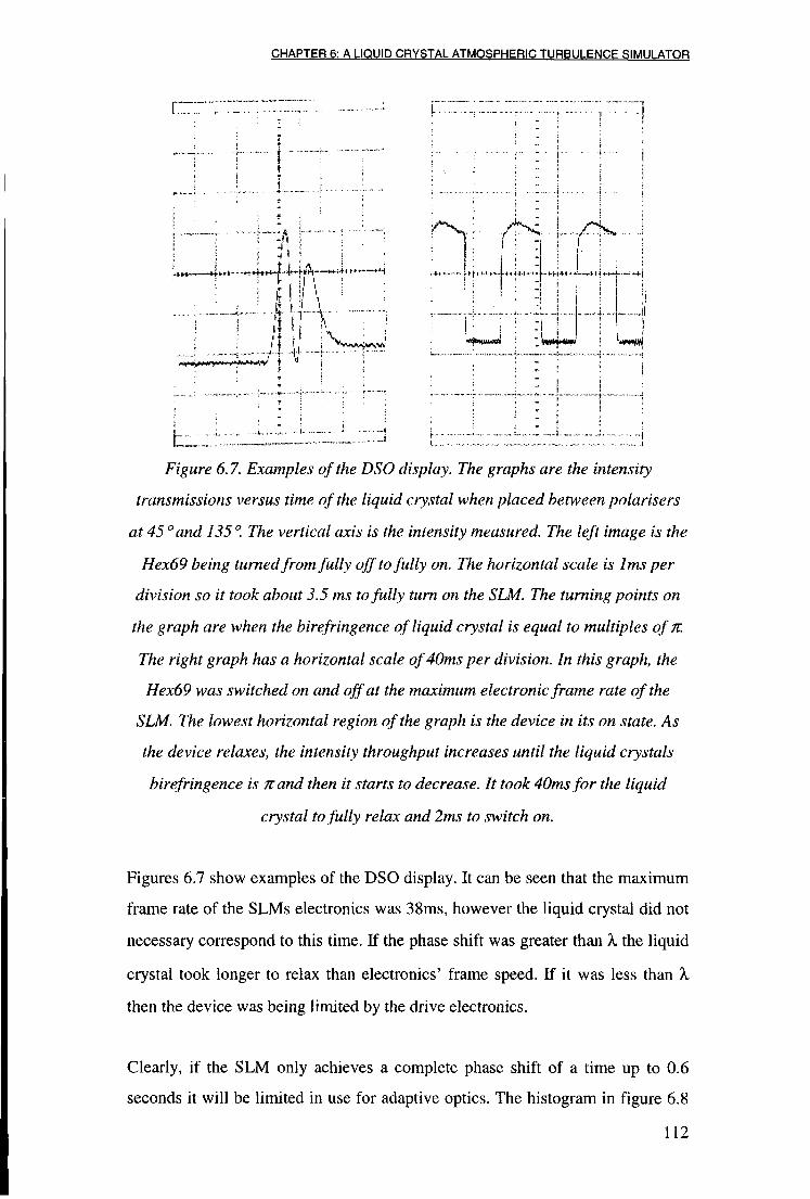
C H A P T E R 6: A L IQUID C R Y S T A L A T M O S P H E R I C T U R B U L E N C E S I M U L A T O R
I I < ' i i ; h , ilt-rl^-- -r+<+»H4- iiH4A~-•**+«
: : M M ; i j I f \ \ \ ; .
rN-; ; -v • i : - ! I
* t • *' * . . ; ,U.w, | | | .
Figure 6.7. Examples of the DSO display. The graphs are the intensity
transmissions versus time of the liquid crystal when placed between polarisers
at 45 "and 135 °. The vertical axis is the intensity measured. The left image is the
Hex69 being turned from fully off to fully on. The horizontal scale is 1ms per
division so it took about 3.5 ms to fully turn on the SLM. The turning points on
the graph are when the birefringence of liquid crystal is equal to multiples of m
The right graph has a horizontal scale of 40ms per division. In this graph, the
Hex69 was switched on and off at the maximum electronic frame rate of the
SLM. The lowest horizontal region of the graph is the device in its on state. As
the device relaxes, the intensity throughput increases until the liquid crystals
birefringence is wand then it starts to decrease. It took 40ms for the liquid
crystal to fully relax and 2ms to switch on.
Figures 6.7 show examples of the DSO display. It can be seen that the maximum
frame rate of the SLMs electronics was 38ms, however the liquid crystal did not
necessary correspond to this time. If the phase shift was greater than X the liquid
crystal took longer to relax than electronics' frame speed. If it was less than X
then the device was being limited by the drive electronics.
Clearly, if the SLM only achieves a complete phase shift of a time up to 0.6
seconds it will be limited in use for adaptive optics. The histogram in figure 6.8
112
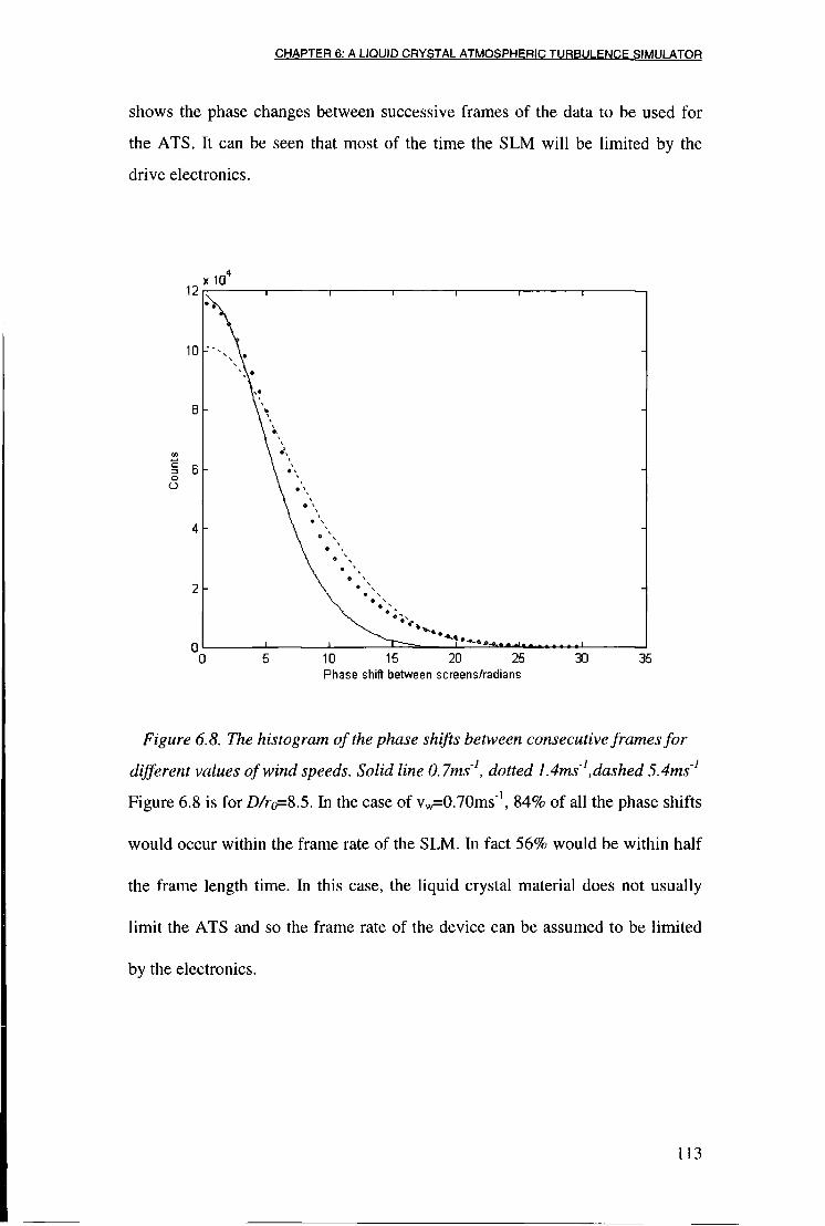
C H A P T E R 6: A L IQUID C R Y S T A L A T M O S P H E R I C T U R B U L E N C E S I M U L A T O R
shows the phase changes between successive frames of the data to be used for
the ATS. It can be seen that most of the time the SLM will be limited by the
drive electronics.
x 104
2
10
8
5 20 25 30 0 35 Phase shift between screens/radians
Figure 6.8. The histogram of the phase shifts between consecutive frames for
different values of wind speeds. Solid line 0.7ms'1, dotted 1.4ms'1 .dashed 5.4ms'1
Figure 6.8 is for D/r0=8.5. In the case of vw=0.70ms"', 84% of all the phase shifts
would occur within the frame rate of the SLM. In fact 56% would be within half
the frame length time. In this case, the liquid crystal material does not usually
limit the ATS and so the frame rate of the device can be assumed to be limited
by the electronics.
113
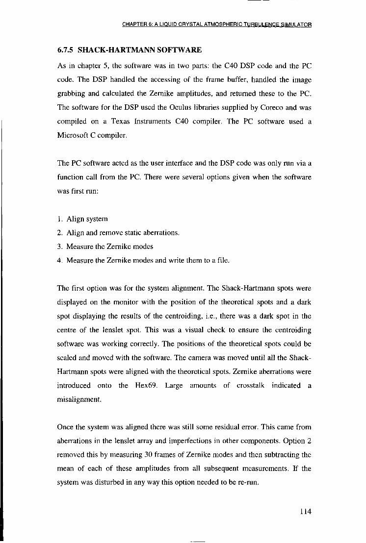
C H A P T E R 6: A L IQUID C R Y S T A L A T M O S P H E R I C T U R B U L E N C E S I M U L A T O R
6.7.5 SHACK-HARTMANN SOFTWARE
As in chapter 5, the software was in two parts: the C40 DSP code and the PC
code. The DSP handled the accessing of the frame buffer, handled the image
grabbing and calculated the Zernike amplitudes, and returned these to the PC.
The software for the DSP used the Oculus libraries supplied by Coreco and was
compiled on a Texas Instruments C40 compiler. The PC software used a
Microsoft C compiler.
The PC software acted as the user interface and the DSP code was only run via a
function call from the PC. There were several options given when the software
was first run:
1. Align system
2. Align and remove static aberrations.
3. Measure the Zernike modes
4. Measure the Zernike modes and write them to a file.
The first option was for the system alignment. The Shack-Hartmann spots were
displayed on the monitor with the position of the theoretical spots and a dark
spot displaying the results of the centroiding, i.e., there was a dark spot in the
centre of the lenslet spot. This was a visual check to ensure the centroiding
software was working correctly. The positions of the theoretical spots could be
scaled and moved with the software. The camera was moved until all the Shack-
Hartmann spots were aligned with the theoretical spots. Zernike aberrations were
introduced onto the Hex69. Large amounts of crosstalk indicated a
misalignment.
Once the system was aligned there was still some residual error. This came from
aberrations in the lenslet array and imperfections in other components. Option 2
removed this by measuring 30 frames of Zernike modes and then subtracting the
mean of each of these amplitudes from all subsequent measurements. I f the
system was disturbed in any way this option needed to be re-run.
114

C H A P T E R 6: A L IQUID C R Y S T A L A T M O S P H E R I C T U R B U L E N C E S I M U L A T O R
Option 3 measured the modes and wrote them to the PC screen. Option 4 also
measured the modes but wrote them to a file. It did not display any thing on the
PC or CCD monitors to increase the speed of the system. Figure 6.9 shows the
software flow chart of the system.
Start
Grabhnage *~
Centroid spots
i Calc. modes
*• Align system?
1 Y
Draw alignment marks
i Write modes to
screen i
Remove static aberration i f
required Write to file
N
DSP PC
Figure 6.9. The software flowchart of the Shack-Hartmann system.
6.7.6 CALIBRATION OF S Y S T E M
Each Zernike mode needed to be calibrated. Slight errors in the alignment and
scaling of the system meant that there was a systematic inaccuracy in each mode,
this needed to be calibrated out. Once the system was aligned different Zernike
modes were placed on the Hex69. The first 12 modes were measured with the
Shack-Hartmann. The amplitudes placed on the Hex69 were -0.5A,, -0.25A., OX,
115

C H A P T E R 6: A L IQUID C R Y S T A L A T M O S P H E R I C T U R B U L E N C E S I M U L A T O R
0. 25.. and 0.5?i. By plotting these amplitudes against the measured amplitude a
calibration line was calculated. This was then added to the PC software so that
all future measurement would be correct.
6.7.7 S Y S T E M LIMITS
The Shack-Hartmann was limited in the largest aberration it could have
measured by either of two factors:
1. The lenslet spots moved out of the search area.
2. The lenslet spots were diffracted by the Hex69 pixels in to more than one
peak.
By drawing a box around the search area it was possible to check that the spots
did not move out side the area. The search areas could have been increased as
long as they did not overlap. They were however kept as small as possible to
increase the speed of the centroiding.
Because the Hex69 is a pixelated device it does cause some diffraction effects.
When the Shack-Hartmann spots were diffracted badly they did not centroid
correctly. This placed the limit on how big the aberration could be. In practice
the limit was -0.8A. for any mode.
The smallest amount detectable was determined by the noise of the system. This
came from environmental perturbations, such as vibrations or camera noise. This
was measured experimentally and the mean RMS noise for all of the modes was
found to be 0.015A,. The RMS noise for each mode is shown in figure 6.10. The
noise on modes 1 and 2 (tip/tilt) is larger than the rest. This is likely to come
from mechanical vibrations in the optical system.
116

C H A P T E R 6: A L IQUID C R Y S T A L A T M O S P H E R I C T U R B U L E N C E S I M U L A T O R
0.1 ra 0.08
0.06 (0
0.04
» 0.02
1 8 9 10 11 Zernike mode
Figure 6.10. The RMS noise limit of each mode.
6.8 Experimental Measurements
6.8.1 T H E Z E R N I K E POWER SPECTRUM
The Zernike power spectrum was measured by placing the Hex69 into the
Shack-Hartmann system. A D/ro = 8.5 was chosen (ro=10cm, Z)=85cm). This
was large enough to give a good signal to noise ratio with the Shack-Hartmann,
but not too large to cause the Shack-Hartmann spots to diffract into more than
one peak. The SLM was run at the maximum frame rate of 38ms (26Hz) and the
Shack-Hartmann's frame rate was 40Hz. This gave 1.5 Shack-Hartmann frames
per Hex69 frame. 4252 measurements were made with the Shack-Hartmann and
the 12 modes each frame generated were written to a file. The RMS for each
mode was then calculated off line. This was compared to a theoretical model by
Wang et al. (Wang, 1977). The power spectrum for the first 12 modes is shown
in figure 6.11. The first two modes are zero because the tip/tilt was removed
from the data.
117

C H A P T E R 6: A L IQUID C R Y S T A L A T M O S P H E R I C T U R B U L E N C E S I M U L A T O R
0.6
0.5
0.4 % (0
£ 0.3 3
a
I 0.2
< 0.1
5 6 7 8 9 10 11
Zernike Mode
12
B Theoretical • Measured
Figure 6.11. The RMS power spectrum of the ATS. This data was taken over
4552frames.
6.8.2 MEASUREMENT OF T E M P O R A L C H A R A C T E R I S T I C S
The Zygo can not measure any temporally varying phase screen because of the
time it takes to grab 5 frames in order to unwrap the phase. A conventional
interferometer could, in principle, be set up with a video camera recording the
interferogram in real time, but this would not address the problem of the phase
ambiguity. To measure a varying phase screen one is generally left with the
option of using a Shack-Hartmann wavefront sensor.
The data was taken in §6.8.1. Figure 6.12 shows the first 10 seconds of mode 3.
It can be seen that there was a large variation over time and that there are no
discontinuities in the data. The wind speed was 0.70ms"1 and D/ra=%.5 (ro=10cm,
Z)=85cm). The exact value of the windspeed depended upon the value chosen for
r0. For the same value of D/ro, but with r0=20cm, the windspeed becomes
1.4ms"1.
118
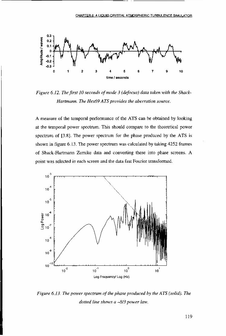
CHAPTER 6: A LIQUID CRYSTAL ATMOSPHERIC TURBULENCE SIMULATOR
S 0.1
i i i
-0.1 £ -0.2
-0.3 0 1 2 3 4 5 6 7 9 10
time / seconds
Figure 6.12. The first 10 seconds of mode 3 (defocus) data taken with the Shack-
Hartmann. The Hex69 ATS provides the aberration source.
A measure of the temporal performance of the ATS can be obtained by looking
at the temporal power spectrum. This should compare to the theoretical power
spectrum of [3.8]. The power spectrum for the phase produced by the ATS is
shown in figure 6.13. The power spectrum was calculated by taking 4252 frames
of Shack-Hartmann Zernike data and converting these into phase screens. A
point was selected in each screen and the data fast Fourier transformed.
-3
10 e . s> • a
-4 10 r
\ 10
5 10
0
8 10
10
10 10
- 2 - 1 0 1
10 10 10 10
Log Frequency/ Log (Hz)
Figure 6.13. The power spectrum of the phase produced by the ATS (solid). The
dotted line shows a -8/3 power law.
119
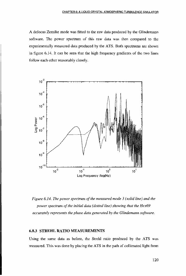
C H A P T E R 6: A LIQUID C R Y S T A L A T M O S P H E R I C T U R B U L E N C E SIMULATOR
A defocus Zernike mode was fitted to the raw data produced by the Glindemann
software. The power spectrum of this raw data was then compared to the
experimentally measured data produced by the ATS. Both spectrums are shown
in figure 6.14. It can be seen that the high frequency gradients of the two lines
follow each other reasonably closely.
10"3
t • — • — • — a
Figure 6.14. The power spectrum of the measured mode 3 (solid line) and the
power spectrum of the initial data (dotted line) showing that the Hex69
accurately represents the phase data generated by the Glindemann software.
6.8.3 STREHL RATIO MEASUREMENTS
Using the same data as before, the Strehl ratio produced by the ATS was
measured. This was done by placing the ATS in the path of collimated light from
10 -4
10
6 10
S 10 I
i 8
10 1
i
10 1
10 10 I
1 0 10 10 10 Log Frequency /log(Hz)
120
C H A P T E R 6: A LIQUID C R Y S T A L A T M O S P H E R I C T U R B U L E N C E SIMULATOR
a red polarised He-Ne laser. This was then focused onto a CCD camera by a
doublet lens. A microscope objective magnified the image of the PSF on the
CCD camera's image plane. It was assumed that when no aberrations were
introduced into the system the PSF was diffraction limited. The Strehl ratio was
defined as being 100% at the peak intensity of this image.
The CCD camera was connected to an FTEX frame grabber. This frame grabber
digitises the CCD images with 8 bit accuracy. It however, has more than one
frame buffer. The TTEX board was programmed to use two frame buffers
together, giving in effect a 16 bit frame buffer. It was then possible to take up to
256 8 bit images and store them in one buffer. Adding all the images together
effectively gives an integrating frame store. It took 0.05 seconds (20Hz) to
process a single frame. The CCD camera was running at 25Hz so some data was
lost.
In the actual Strehl ratio measurement only 200 frames were used (10 seconds of
data) because there was some damage to one of the frame buffers. With the ATS
running, the measured Strehl ratio was 17%.
The theoretical Strehl ratio is commonly defined with equation [3.15]. This
equation is only accurate for a small o. To calculate the theoretical Strehl ratio
the data produced by the Lane and Glindemann software was fast Fourier
transformed and the mean of the 2000 PSFs was taken as the theoretical
expectation. The theoretical Strehl ratio was 11%.
6.9 Discussion
This chapter has developed an ATS using nematic liquid crystals and measured
it performance. It can be seen from figure 6.11 that the system has approximately
the correct RMS value of each Zernike mode for the D/r0 value that was
modelled. The other measure of this was the Strehl ratio. Although this was
slightly higher than was expected, it is possible that the discrepancy comes from
the coarse pixelation of the Hex69 device.
121
C H A P T E R 6: A LIQUID C R Y S T A L A T M O S P H E R I C T U R B U L E N C E SIMULATOR
Figure 6.13 shows a -8/3 power law at high frequency for the phase shifts
produced by the ATS. This is in good agreement with the expected gradient from
equation [3.8].
The study in §6.7.4 showed that the liquid crystal was fast enough to reach the
desired phase shift most of the time within one frame. In figure 6.14 it can be
seen the SLM produces the correct amount of high frequency power. These two
facts suggest that the slow speed of the liquid crystal was not limiting the ATS.
The Hex69 SLM is 9 pixels across. When an aberration with a D/r0 of 8.5 was
used, each Hex69 pixel is approximately modelling one Fried length. It seems
sensible to suggest that this should be the maximum aberration that should be
applied to the ATS. There is no clear cut off since the drop in performance will
be a sliding scale.
The wind speed the ATS was simulating was chosen to be 0.70ms"1. Since the
maximum frame speed is fixed, the only way of increasing this speed is to skip
frames, e.g., only use every second frame, effectively doubling the simulated
wind speed. This has two effects: it increases the decorrelation between frames
and it introduces discontinuities between frames. It can be assumed that these
effects will decrease the accuracy of the ATS. It is not presently known what
would be the maximum effective speed of the ATS. This will require further
experimental work.
The ATS demonstrated has been shown to reasonably model the atmosphere.
The device can be used in testing adaptive optics systems (in chapter 7 for
example). Because of the low cost nature of the SLM it will be possible to
cascade several devices, each representing a layer of turbulence. It should then
be then possible to provide a good aberration source for testing multiconjugate
adaptive optics.
122
C H A P T E R 6: A LIQUID C R Y S T A L A T M O S P H E R I C T U R B U L E N C E SIMULATOR
6.10 Summary An atmospheric turbulence simulator has been demonstrated. This has many
possible applications in testing adaptive optics systems. Now that an
atmospheric turbulence source has been developed it can be used in the next
chapter with the Shack-Hartmann wavefront sensor.
123
C H A P T E R 7: BINARY ADAPTIVE O P T I C S WITH A SHACK -HARTMANN W A V E F R O N T S E N S O R
Chapter 7: Binary Adaptive Optics with a Shack-Hartmann Wavefront Sensor
7.1 Introduction
Chapter 5 demonstrated a binary adaptive optics system using a PDI. Although it
provided good correction there were still various problems associated with the
PDI. There was a low optical throughput, pixel oscillations, and the system took
several frames to reach the best solution. In this chapter a more conventional
wavefront sensor, the Shack-Hartmann, will be used. The ATS system developed
in chapter 6 will be the aberration source.
7.2 Background
Shack-Hartmann wavefront sensors have become the standard sensor in adaptive
optics. They are well understood and there is a large amount of literature (see
(Tyson, 1991), (Beckers, 1993) for examples). They are commercially available
in 'off the shelf packages as complete systems, with all the necessary analysis
software (Ref. AOA). However, these commercially available systems are too
slow for adaptive optics applications (~lHz). It is unlikely that the Shack-
Hartmann should cause the oscillations seen in chapter 5 and the complete
system should also reach the correct solution in the first frame. It also has the
advantage that there are many Shack-Hartmann systems already built for
adaptive optics systems on other telescopes. A laboratory based system could
easily be modified to use this equipment so that there would be no need to ship
our wavefront sensor to a telescope. It is not unreasonable to assume that most
telescopes' Shack-Hartmann cameras will work better with starlight than our
laboratory camera, which was not optimised for low light.
124

C H A P T E R 7: BINARY ADAPTIVE O P T I C S WITH A SHACK -HARTMANN W A V E F R O N T S E N S O R
7.3 Experimental System
7.3.1 OPTICAL SET-UP
LA CCD! Laser
Figure 7.1. The optical set-up. LI, L2, L3, L4 are doublet lenses; M is the Hex69
SLM which was used to generate optical aberrations; WP is a half wave plate;
BS is a beam splitter; FLC is the Displaytech FLC which provided the wavefront
correction; POL is a polariser; CCD1 is the Shack-Hartmann CCD camera;
CCD2 is the science camera; and LA is the lenslet array. L2 and L3 demagnify
the beam so that the Hex69 pixels map onto the lenslet array.
The experimental system is shown in figure 7.1. The system is similar to that in
chapter 6 except for the addition of the FLC system. A polarised lOmW He-Ne
laser was used so that only one polariser was needed. The laser was polarised
along the extraordinary axis of the Hex69. The Hex69 acted as the source of
optical aberrations, the ATS. The system was in open loop because when the
FLC was tried in a closed loop the inter-pixel gaps of the FLC blocked out some
of the Shack-Hartmann spots. Unfortunately this made the alignment of the
system considerably harder. The two lenses, L2 and L3, demagnified the beam to
the size of the lenslet array, LA.
125
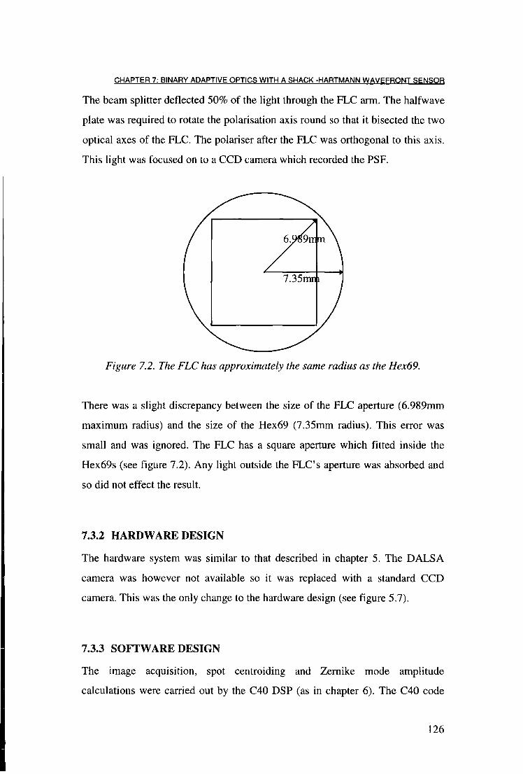
C H A P T E R 7; BINARY ADAPTIVE O P T I C S WITH A SHACK -HARTMANN W A V E F R O N T S E N S O R
The beam splitter deflected 50% of the light through the PLC arm. The halfwave
plate was required to rotate the polarisation axis round so that it bisected the two
optical axes of the FLC. The polariser after the FLC was orthogonal to this axis.
This light was focused on to a CCD camera which recorded the PSF.
Figure 7.2. The FLC has approximately the same radius as the Hex69.
There was a slight discrepancy between the size of the FLC aperture (6.989mm
maximum radius) and the size of the Hex69 (7.35mm radius). This error was
small and was ignored. The FLC has a square aperture which fitted inside the
Hex69s (see figure 7.2). Any light outside the FLC's aperture was absorbed and
so did not effect the result.
7.3.2 HARDWARE DESIGN
The hardware system was similar to that described in chapter 5. The DALSA
camera was however not available so it was replaced with a standard CCD
camera. This was the only change to the hardware design (see figure 5.7).
7.3.3 SOFTWARE DESIGN
The image acquisition, spot centroiding and Zernike mode amplitude
calculations were carried out by the C40 DSP (as in chapter 6). The C40 code
7.35mm
126

C H A P T E R 7: BINARY ADAPTIVE O P T I C S WITH A SHACK -HARTMANN W A V E F R O N T S E N S O R
had to be altered to work with the CCD camera. The previous method of separating the 32 bit words in to the four 8 bit intensity values by grabbing the image and copying it into the F/64's RAM would not work. This was because the image from the CCD camera was larger than the F/64's RAM. Instead, a function call was written to access each pixel directly from the frame buffer. The other modification to be made was to the centroiding algorithm. The CCD camera did not have square pixels, but pixels with a 3:4 width:length ratio as in a TV. The position of the pixels sampled was modified to remove the biasing in one direction caused by the rectangular shape of the pixels. The CCD pixels were also smaller than the DALSA so the search box area for the centroiding had to be increased to 50x50 pixels.
The PC code was also based on the code from the last chapter. The Zernike
modes were returned to the PC from the DSP as before. The system was aligned
and two new options were added:
1. Correct with diagnostics
2. Correct without diagnostics
The diagnostics option caused the measured modes to be printed to the PC
screen and display the position of the centroid spots on the camera monitor, as
well as perform the correction of the aberrations. This only had a bandwidth of
~lHz. Option 2 did not display any information. The bandwidth of the system
was 6Hz. This is considerably slower than the similar system in chapter 6
because of the large amount of image data to process, and the slowness of
accessing each pixel with a function call. If the system was not limited by the
computation, the fundamental limit would of been that of the camera, 25Hz.
The correction algorithm was as follows.
127
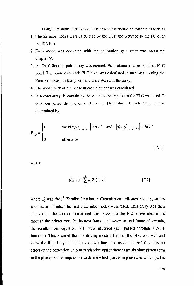
C H A P T E R 7: BINARY ADAPTIVE O P T I C S WITH A SHACK -HARTMANN W A V E F R O N T S E N S O R
1. The Zernike modes were calculated by the DSP and returned to the PC over the ISA bus.
2. Each mode was corrected with the calibration gain (that was measured
chapter 6).
3. A 10x10 floating point array was created. Each element represented an FLC
pixel. The phase over each FLC pixel was calculated in turn by summing the
Zernike modes for that pixel, and were stored in the array.
4. The modulo 2% of the phase in each element was calculated.
5. A second array, P, containing the values to be applied to the FLC was used. It
only contained the values of 0 or 1. The value of each element was
determined by
for <Kx>y) modulo 2K >n/2 and <Kx>y) modulo 2TC < 371/2
otherwise
[7.1]
where
ix,y)=Y,ajZj{x,y) [7.2]
where Zj was the / h Zernike function in Cartesian co-ordinates x and y, and ay
was the amplitude. The first 8 Zernike modes were used. This array was then
changed to the correct format and was passed to the FLC drive electronics
through the printer port. In the next frame, and every second frame afterwards,
the results from equation [7.1] were inversed (i.e., passed through a NOT
function). This ensured that the driving electric field of the FLC was AC, and
stops the liquid crystal molecules degrading. The use of an AC field has no
effect on the correction. In binary adaptive optics there is no absolute piston term
in the phase, so it is impossible to define which part is in phase and which part is
128
C H A P T E R 7: BINARY ADAPTIVE O P T I C S WITH A S H A C K -HARTMANN W A V E F R O N T S E N S O R
out. The addition of % radians to a pixel in frame 1 is equivalent to the addition of -71 in frame 2. When using an FLC, one is only concerned with the phase difference between on and off pixels not the absolute phase.
7.3.4 OPEN LOOP CONSIDERATIONS
The Shack-Hartmann lenslet array used in this system had a hexagonal format.
There was therefore, a mismatch between the sampling area of the lenslet and
the FLC pixel areas. The interpixel gaps also posed problems by interfering with
the spots when the FLC was placed in front of the lenslet array. For this reason
the device was run in open loop. This presented two problems to be overcome.
1. There was no feedback. If the device were in a closed loop the system would
always tend towards the correct solution even if the calibration was not
accurate. In an open loop system the lack of feedback means that any error in
the measurement will not be corrected.
2. The alignment of the system was more difficult. Because of the lack of
feedback there was no easy way of testing if the system was correctly aligned.
In a closed loop system, an aberration could be applied to the FLC and
measured with the Shack-Hartmann. This would have also ensured that the
FLC was orientated correctly, i.e., it was not back-to-front, upside down, or
rotated, etc.
However, the lack of feedback was not critical once the system was aligned
because of the binary nature of the system. It was expected that any phase
measurement errors would be less than it radians. Any additional accuracy was
not needed in this system.
129
C H A P T E R 7: BINARY ADAPTIVE O P T I C S WITH A S H A C K -HARTMANN W A V E F R O N T S E N S O R
7.3.5 ALIGNMENT
The Hex69 was easier to align then the FLC. Zernike modes could be applied to
the Hex69 and these were measured with the Shack-Hartmann. Any rotational
misalignments (in units of 90°) could be corrected in the Shack-Hartmann
software, for example, if Zernike mode 1 was applied but only mode 2 was
measured this could be corrected by changing the order of the modes in the
software.
The alignment of the FLC was much more difficult. This was done by taking
advantage of the liquid crystal SLMs' birefringence. By using polarisers at the
correct angles, the SLMs were used as intensity modulators. The steps involved
applying a Zernike mode, such as astigmatism, to the Hex69. This was measured
with the Shack-Hartmann and this measured amplitude was also applied to the
FLC. A polariser at 45° to the Hex69's optical axis was then placed before the
Hex69, and one at 135° was placed after. This made the SLM an intensity
modulator. The orientation of the Zernike mode on the FLC was then checked in
a similar manner. This was repeated for all modes. The magnification of the
system can be checked with defocus. A defocus mode applied to the FLC should
produce a dark ring. The Hex69 and FLC have slightly different sizes so the
scale factor in the software was altered to compensate for this.
7.3.6 PREDICTED PERFORMANCE
The FLC used in this chapter is the same as in chapter 6, so it suffered from the
same problems of having a small number of pixels. The expected performance of
the system can however be calculated. The wavefront error after correction
depends on several factors. Let a 2 be the residual wavefront error after
correction. This is calculated from
a2 =a2
W F S + o L +o^m + oLp [7.3]
130

C H A P T E R 7: BINARY ADAPTIVE O P T I C S WITH A SHACK -HARTMANN W A V E F R O N T S E N S O R
where C W F S is the wavefront sensor error, oCOn is the fitting error of the wavefront corrector, Ozem is the residual error from the high order Zernike modes not corrected, and atemp is the error from the finite speed of the system.
An estimate for the wavefront sensor error can be derived from the
measurements of the Shack-Hartmann noise. The contribution for each mode's
noise to the total variance was calculated. Software was written to calculate the
phase at 100 points, corresponding to each FLC pixel. The variance in phase was
then calculated from the noise at these discrete points. This was calculated to be
0.0013 radians2.
It is not possible for any deformable mirror or liquid crystal SLM to completely
match the aberrations produced by the atmosphere. There will always be some
wavefront error after correction from the corrector's inability to completely fit
the wavefront. Hudgin (Hudgin, 1997) developed a formula for the fitting error
given by
( \ r.
V r o J
5A [7.4]
where rs is the distance between actuators and a is called the fitting parameter.
He calculated various values for a with different types of mirror. For a Gaussian
response a=0.28, for a pyramidal response a=0.23 and for a piston only
response, a=1.26. The FLC can be considered to behave like a piston only
mirror so a=1.26 was chosen, however there is also an additional fitting error
from the FLCs binary operation. If we consider some phase function over the
aperture, (|)(x), where x is the two dimensional vector, in binary adaptive optics
we are only concerned with <|)(x) being in the range of 0 to 2n radians. For a
(large) normal random distribution, after correction the mean phase is (|)(x) =7t/2
131

CHAPTER 7: BINARY ADAPTIVE OPTICS WITH A SHACK -HARTMANN WAVEFRONT SENSOR
and <|)(x) can vary from 0 to % radians. The variance wavefront error from the
FLC, O~FLC, is
< C = ( [ < K * ) - * ] 2 } [7.5]
= 0.824 radians2
This assumes that <j)(x) varies uniformly between 0 and 2%. Since the FLC can be
considered to have a piston response with a residual error given by [7.5], the
total value for acon is
+ 0.824 [7.6]
for D/r0 =8.5 and D/rs=\0 for the FLC, [7.6] equals 1.785 radians2.
The wavefront error from the limited number of Zernike modes corrected is
given by Noll (Noll, 1976). If the first eight modes are corrected (see table 3.3)
< „ = 0 . 0 4 6 3 ( % J % [7.7]
= 1.639 radians
There was also an error from the finite speed of the corrector system, a t e mp-
Tyson (Tyson, 1991) shows that
temp
f \ 0.4v
V r o fc J
[7.8]
132

C H A P T E R 7: BINARY ADAPTIVE O P T I C S WITH A SHACK -HARTMANN W A V E F R O N T S E N S O R
where v is the wind velocity (taken as 5ms"1) and/ c is the bandwidth of the system. If/c=40Hz and r0=10cm, [7.8] equals 0.5 radians2.
For D/r0=$.5, the uncorrected variance is 4.7 radians2 (with tip/tilt removed).
The total expected residual wavefront error after correct has been calculated as
3.92 radians2.
7.4 Results
The correction performance was measured in terms of Strehl ratio. The PSFs
were measured with the CCD 2 camera (figure 7.1). This was used in
conjunction with the ITEX integrating frame grabber (see chapter 6).
7.4.1 STATIC CORRECTION
An example of static correction is shown in figures 7.3, 7.4 and 7.5. An
aberration was applied to the Hex69. The uncorrected PSF is shown in figure
7.4, the Strehl ratio was 30%. The corrected PSF is shown in figure 7.5, with a
Strehl ratio of 48%. This is an improvement in a factor of 1.6. Figure 7.6 shows
the actual PSF images.
133
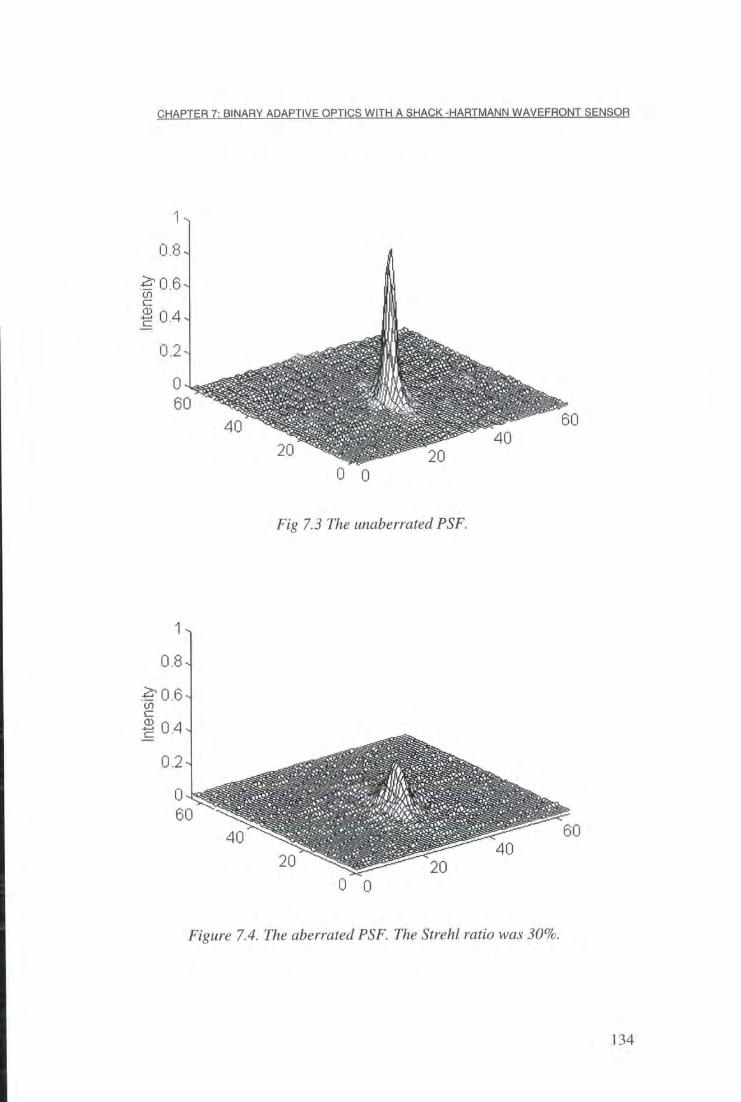
0HAPTF_R.7^INARY_ADAPTIVE OPTICS WITH A SHACK -HARTMANN WAVEFRON1 SENSOR
0 8
^ 0 . 6 m . l i
0 . 4
0 . 2
6 0
6 0 4 0
4 0 2 0 2 0
0 0
Fig 7.3 The unaberrated PSF.
U
0 . 8 .
. ^ 0 . 6 ^
04
0 . 2
0 4 ?
60 6 0
4 0 4 0
2 L) 2 0
0 0
Figure 7.4. The aberrated PSF. The Strehl ratio was 30%.
1 3 4

C H A P T E R 7: B I N A R Y A D A P T I V E O P T I C S W I T H A S H A C K - H A R T M A N N W A V E F R O N T S E N S O R
1
0 . 8
^ 0 . 6 IJ
a.' 0 . 4
0 . 2
0
6 0
6 0 40 4 0
2 0 2 0
0 0
Figure 7.5. The corrected PSF. The Strehl ratio was 48%
Figure 7.6. From left to right, the unaberrated, the aberrated and the corrected
PSFs.
7.4.2 REAL TIME CORRECTION
The ATS system developed in chapter 6 was used as the aberrator for the real
time correction system. The phase data was scaled to give a D/r0 of 8.5. Because
of the slow speed of the Shack-Hartmann (6Hz) the wind speed was reduced to
135
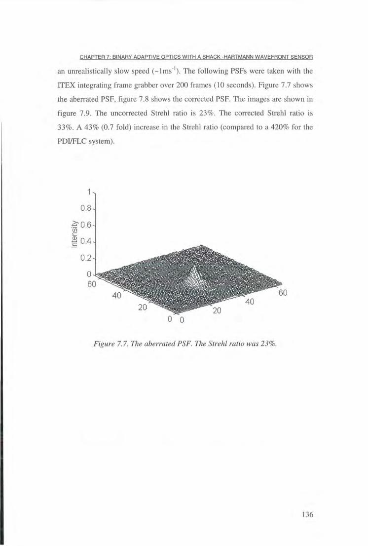
CHAPTER 7: BINARY ADAPTIVE OPTICS WITH A SHACK -HARTMANN WAVEFRONT SENSOR
an unrealistically slow speed (~lms _ l). The following PSFs were taken with the ITEX integrating frame grabber over 200 frames (10 seconds). Figure 7.7 shows the aberrated PSF, figure 7.8 shows the corrected PSF. The images are shown in figure 7.9. The uncorrected Strehl ratio is 23%. The corrected Strehl ratio is 33%. A 43% (0.7 fold) increase in the Strehl ratio (compared to a 420% for the PDI/FLC system).
1
0.8
^0 .6
0.4
0.2
0 60
tiU 40 40
20 20 0 0
Figure 7.7. The aberrated PSF. The Strehl ratio was 23°Ii
136
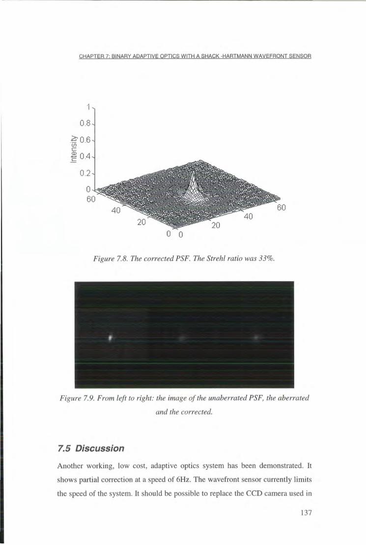
CHAPTER 7: BINARY ADAPTIVE OPTICS WITH A SHACK -HARTMANN WAVEFRONT SENSOR
1
0.8
^ 0 . 6 n
a.. 0.4
0.2
0 60
60 40 40
20 20 0 0
Figure 7.8. The corrected PSF. The Strehl ratio was 33°7t c.
Figure 7.9. From left to right: the image of the unaberrated PSF, the aberrated
and the corrected.
7.5 Discussion Another working, low cost, adaptive optics system has been demonstrated. It
shows partial correction at a speed of 6Hz. The wavefront sensor currently limits
the speed of the system. It should be possible to replace the CCD camera used in
137

C H A P T E R 7: B I N A R Y A D A P T I V E O P T I C S W I T H A S H A C K -HARTMANN W A V E F R O N T S E N S O R
this experiment with the high speed DALSA camera. There is no reason why this system should not then work at the frame rate (40Hz) of the Shack-Hartmann used in chapter 6. The drop in the frame rate was because of the camera's lower speed (25Hz) and large number of pixels to process (768 by 575 compared to 128 by 128 for the DALSA). The Shack-Hartmann system has been tested on a 200MHz Pentium system with the DALSA camera; the frame rate of the system was then increased to 60Hz. At such frame rates the device is approaching speeds that would be useful in astronomical applications.
In common with the FLC/PDI system in chapter 5, the transmission of the FLC
is prohibitively low for astronomical applications (2%). However, this system
does have the advantage of having a more light efficient wavefront sensor. The
Shack-Hartmann camera was not optimised for low light conditions but such
systems are in use on telescopes.
A method of improving the transmission of the FLC would be to operate it at a
different wavelength so that its retardance was n radians. The theoretical
transmission of the SLM and the two polarisers (excluding absorption and
reflections) would then be 50%. The Meadowlark polariser used in this
experiment has a quoted transmission of 42% in unpolarised light, or an 8% loss
in polarised light. The expected transmission with the two polarisers and the
FLC with a retardance of n would then be 33%. Although lossy, it is
considerably better than the measured value used in this experiment. The
wavelengths that give it radians retardance for this device are 383nm (in the UV)
or 1659nm (in the IR). However, if UV light was used the atmospheric
turbulence would be more severe, and the transmission characteristics of the
device are not known at either of these two wavelengths.
The measured correction was lower than the possible increase in Strehl ratio to
40.5%. Part of this performance drop has been quantified in equation [7.3].
There was always some residual error because of the finite capabilities of the
138

C H A P T E R 7: B I N A R Y A D A P T I V E O P T I C S WITH A S H A C K - H A R T M A N N W A V E F R O N T S E N S O R
system. From [7.3] it can be seen that the greatest contribution to this comes from the G c o r r term given by equation [7.6]. In binary adaptive optics there will always be the 0.824 factor, however the left hand part of [7.6] (i.e., [7.4]) still contributes 0.96 radians2. A modest increase in the number of pixels to say 15 by 15 would reduce this number by a half.
The other major quantifiable contribution to the error in correction is from the
number of Zernike modes used to describe the wavefront. Completely correcting
the first eight modes still leaves a wavefront variance of 1.639 radians2. This is a
large fraction of the total residual error and is much larger than the error from the
finite speed of the system. If the system was to be operated with the high speed
DALSA camera it is clear that more Zernike modes should be calculated even at
the expense of system speed. If we consider the frame speed of the system to be
40Hz, the variance of the system from the temporal residual error is 0.5 radians2
(from [7.8]). For a ^ m to equal this requires the first 34 modes to be corrected
(from [3.14]). There is clearly some room in the future for the optimisation of
the system by balancing the number of modes calculated with the frame speed of
the system. It should be noted that because only 19 lenslets are used, only the
first 38 modes could be calculated. Redesigning the optics could increase this,
but the Hex69 could then no longer be used as the ATS.
The other possible source of error is from misalignment of the optics. The exact
contribution this causes is difficult to quantify. The most likely source of error
comes from the positioning of the FLC in the system. The exact alignment is
difficult because of the small size of the pixels. In the worse case, the FLC could
be out of alignment by one pixel. This could cause the Strehl ratio to decrease
when correction was attempted.
Using the FLC with a Shack-Hartmann has several advantages over the Smartt
PDI system in chapter 5. The Shack-Hartmann has a considerably higher light
efficiency. Except for losses from absorption by the glass components there is no
139

C H A P T E R 7: B I N A R Y A D A P T I V E O P T I C S WITH A S H A C K - H A R T M A N N W A V E F R O N T S E N S O R
attenuation with the Shack-Hartmann system. The number of photons required by a Shack-Hartmann is well documented (Cao, 1994).
Because of the system's open loop nature there were none of the pixel
oscillations that were seen with the PDI system, and the solution is found in the
first frame. This means that the wavefront sensor does not have to be operated as
fast as the PDI sensor for a given aberration. This also improves the overall light
efficiency of the system.
When used in binary adaptive optics the Shack-Hartmann actually provides more
information than is needed. In binary adaptive optics the only information
needed is whether a pixel is in or out of phase relative to another pixel.
However, using the Shack-Hartmann means that the system is easily modified
for quarter wave correction. This is impossible with the PDI system in chapter 5,
unless a phase shifting PDI is used. Since these devices rely on nematic liquid
crystals, they will always be slow compared to what can be achieved with a
Shack-Hartmann.
To achieve quarter wave correction with PLCs for astronomy, devices with
higher switching angles will have to be developed. When used with polarisers,
PLCs have too low a transmission for astronomical applications. Assuming that
a high switching angle FLC would have a similar transmission to the
Displaytech FLC, two cascaded together to give quarter wave switching would
have a transmission of -0.8 2 = 64%, which is still low but usable.
With quarter wave switching it is expected that the Strehl ratio improvement in
an experiment similar to one in this chapter would be better. The maximum
correction achievable from a binary corrector is 40.5%. It is unlikely that FLCs
will ever compete with deformable mirrors unless used as at least quarter wave
correctors. This would enable correction up to a Strehl ratio of 81%.
140

C H A P T E R 7: B I N A R Y A D A P T I V E O P T I C S WITH A S H A C K - H A R T M A N N W A V E F R O N T S E N S O R
With quarter wave correction [7.6] becomes
+ 0.206 [7.9]
2 2
If we define a system to be well corrected when a <1 radians . This happens
when r,<0.75 r 0. To achieve a Strehl ratio of 80% we require rs=0.08 r 0.
Like in chapter 5, the system is limited by transmission. Assuming this problem
could be addressed the next stage of constructing a future system would be to
improve the frame speed of the system and calculate more Zernike modes. The
system could then be tried on a real telescope.
Until high switching angle FLC materials are developed, it is unlikely that FLCs
will be of much use in astronomical adaptive optics systems. At present, nematic
liquid crystal SLMs have two major advantages: their high transmission and the
ability to fully correct an aberration.
7.6 Summary In this chapter an FLC adaptive optics system with a Shack-Hartmann wavefront
sensor has been constructed. The real time speed was limited to 6Hz due to
equipment problems but an increase in the Strehl ratio from 23% to 33% was
measured. This was a real time measurement over a period of 10 seconds.
It has been demonstrated in this chapter (and chapter 5) that an FLC does
provide partial correction in real time. However, their limited throughput makes
them unsuitable for atmospheric systems at present. For this reason the next
chapter will describe a nematic liquid crystal SLM which will be used as the
corrector. Although nematic liquid crystals have a slower speed they have a far
higher transmission and perform complete analogue correction.
141
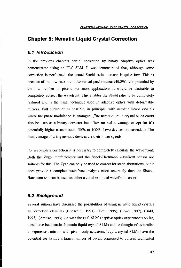
C H A P T E R 8: N E M A T I C L IQUID C R Y S T A L C O R R E C T I O N
Chapter 8: Nematic Liquid Crystal Correction
8.1 Introduction
In the previous chapters partial correction by binary adaptive optics was
demonstrated using an FLC SLM. It was demonstrated that, although some
correction is performed, the actual Strehl ratio increase is quite low. This is
because of the low maximum theoretical performance (40.5%), compounded by
the low number of pixels. For most applications it would be desirable to
completely correct the wavefront. This enables the Strehl ratio to be completely
restored and is the usual technique used in adaptive optics with deformable
mirrors. Full correction is possible, in principle, with nematic liquid crystals
where the phase modulation is analogue. (The nematic liquid crystal SLM could
also be used as a binary corrector but offers no real advantage except for it's
potentially higher transmission- 50%, or 100% if two devices are cascaded). The
disadvantage of using nematic devices are their lower speeds.
For a complete correction it is necessary to completely calculate the wave front.
Both the Zygo interferometer and the Shack-Hartmann wavefront sensor are
suitable for this. The Zygo can only be used to correct for static aberrations, but it
does provide a complete wavefront analysis more accurately then the Shack-
Hartmann and can be used as either a zonal or modal wavefront sensor.
8.2 Background
Several authors have discussed the possibilities of using nematic liquid crystals
as correction elements (Bonaccini, 1991), (Dou, 1995), (Love, 1997), (Bold,
1997), (Amako, 1993). As with the FLC SLM adaptive optics experiments so far,
these have been static. Nematic liquid crystal SLMs can be thought of as similar
to segmented mirrors with piston only actuators. Liquid crystal SLMs have the
potential for having a larger number of pixels compared to current segmented
142

C H A P T E R 8: N E M A T I C L IQUID C R Y S T A L C O R R E C T I O N
mirrors, but segmented mirrors are typically driven with three actuators giving movement in the direction of tip, tilt and piston. This gives them three degrees of freedom per pixel/mirror compared to one degree for a nematic liquid crystal SLM pixel. This has been addressed with computer simulations by Bonaccini et. al. (1991). Their model suggested that to get a good correction (Strehl ratio >0.8) 26x26 nematic SLM pixels are needed, whereas only 10x10 tip/tilt/piston actuators are needed for aZ>=3.5m and r0=0.4m (Z)/r0=8.75).
8.3 Device Description
The nematic SLM used in this chapter was the Meadowlark Hex69. A ful l
description of the device is given in §6.5.
8.3.1 D R I V I N G S O F T W A R E
To control the device three programs were used. The first two were for static
control of the device. These programs could either control individual pixel values
or added Zernike modes. The third was a modified version of the Shack-
Hartmann software used in §6.7.5 and §7.3.3 and was used to perform the real
time correction. This program is described below.
8.4 Static Correction
To assess how well the Hex69 can shape wavefronts static corrections are useful.
The wavefront measurements were done with the Zygo interferometer. The Zygo
produced a data file containing 196 by 226 data points. To locate the Hex69
pixels on the interferogram a map file was generated. This was done by setting
the voltages of all the Hex69 pixels to 0V and increasing one pixel until there
was a dark fringe on the pixel in the Zygo's display screen. This interferogram
was saved to disk and the process repeated for all the Hex69 pixels. The 69 files
were then thresholded to determine where the dark pixel was. A calibration file
143

CHAPTER 8: NEMATIC LIQUID CRYSTAL CORRECTION
was then produced containing the position of each Hex69 pixel on the interferogram. This is shown in figure 8.1
r
Figure 8.1. A grey scale representation of the calibration map file.
Using this map file it was then possible to calculate the phase over any given
Hex69 pixel from the Zygo, providing the Hex69 was not moved.
An aberrating piece of glass was placed in front of the Hex69 in the Zygo system
(see figure 8.2). The phase screen was then measured with the Zygo. This file
was saved and the required phase shift for each pixel needed to correct the
aberration induced by the glass was calculated off line. The Zygo calculated the
Strehl ratios before correction and after correction by Fourier transforming the
phase data. The improvement is shown in table 8.1. The aberrated and corrected
wavefronts are shown in figure 8.3 and in figure 8.4.
144
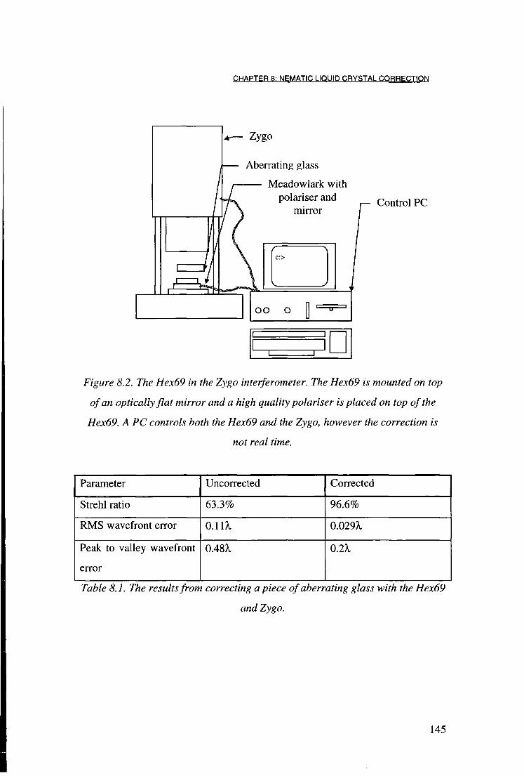
C H A P T E R 8: N E M A T I C L IQUID C R Y S T A L C O R R E C T I O N
Zygo
Aberrating glass
Meadowlark with polariser and Control PC
mirror
r
• o o
Figure 8.2. The Hex69 in the Zygo interferometer. The Hex69 is mounted on top
of an optically flat mirror and a high quality polariser is placed on top of the
Hex69. A PC controls both the Hex69 and the Zygo, however the correction is
not real time.
Parameter Uncorrected Corrected
Strehl ratio 63.3% 96.6%
RMS wavefront error o.i a 0.029A.
Peak to valley wavefront
error
0.48A. 0.2A.
Table 8.1. The results from correcting a piece of aberrating glass with the Hex69
and Zygo.
145

CHAPTER 8: NEMATIC LIQUID CRYSTAL CORRECTION
Figure 8.3. The left is the uncorrected phase map of a piece of glass. The right is
the corrected phase map by the Hex69. The pixelation of the Hex69 is clearly
visible.
m 1 m
n •
• !
Figure 8.4. The left graph is the uncorrected phase graph. The right graph is the
corrected. The sharp peaks on the corrected phase graph are from bad data
points measured by the Zygo. Ignoring these points will greatly improve the peak
to valley measurement.
146
C H A P T E R 8: N E M A T I C L IQUID C R Y S T A L C O R R E C T I O N
The Zygo takes about 20 seconds to process the data and the whole process takes of the order of a minute so this is in no way a real time system. It does demonstrate the correction ability of nematic liquid crystal SLMs.
8.4.1 S T A T I C Z E R N I K E C O R R E C T I O N
To access how well the Hex69 could correct for simulated data, Zernike modes
were added to the raw measured data with the Zygo. Using this it was possible to
add imaginary aberrations into the system. The Zygo added various Zernike
modes to the data and the software attempted to correct them. This was really a
measurement of how well the Hex69 could generate Zernike modes using the
Strehl ratio as a measure of performance.
Various Zernike mode amplitudes were added into the data and the Hex69
attempted to correct for these. The Zygo measured the mode applied to the Hex69
and added the software data to this. If the two were exactly conjugate the Zygo
should measure a flat wave and the Strehl ratio would be restored to 100%. The
before and after Strehl ratios are shown in figure 8.5 for an amplitude of A/4 and
figure 8.6 for an amplitude of A/2. The corrected Strehl ratios in figure 8.5 are all
above 90% (except mode 8), so the residual wavefront variance is less than 0.3
radians. In this case the Strehl ratio is defined as being the ratio of the measured
and diffraction limited intensities at the DC term. This is so that the performance
of correcting tip and tilt could be assessed.
147

C H A P T E R 8: N E M A T I C L IQUID C R Y S T A L C O R R E C T I O N
1 i
0.8 •
0.6
0.4
0.2 l l l l l l l l • Aberrated • Corrected
£ V> £ < <
Zernike Mode
Figure 8.5. The aberrated and corrected Strehl ratios from simulated data. The
amplitude of the Zernike modes was X/4
1 n
0.8
a_n 2 I I CM
at
CO
• Aberrated B Corrected
Zernike Mode
Figure 8.6. The aberrated and corrected Strehl ratios from simulated data. The
amplitude of the Zernike modes was A/2. Defocus, astigmatism 1, coma 1 and 2
and spherical are incorrect because the Zygo could not measure the aberration
produced by the Hex69 due to the coarse pixelation so no reliable results were
possible for these modes at this amplitude.
In figure 8.6 the limitation of the correction was not the Hex69, but the Zygo's
difficulty in measuring coarsely pixelated wavefronts.
148

C H A P T E R 8: N E M A T I C L IQUID C R Y S T A L C O R R E C T I O N
8.4.2 M O D A L C R O S S T A L K M E A S U R E M E N T S
Zernike modes of various amplitudes were applied to the Hex69. These were
measured with the Zygo. The Zygo fits Zernike modes to the data by using a
least-square-fitting algorithm. The measured modes are shown in figures 8.7 to
8.15. They were also measured with the Shack-Hartmann in §8.5.3. It can be seen
that there was considerable crosstalk between certain modes. This happens
between similar modes, that is, between a low order mode and its higher order
equivalent. This can be clearly seen when 0.25A. of spherical aberration (mode 8)
was applied and -0.11 A, of defocus (mode 3) and -0.14A. of high order spherical
(mode 15) was measured. Only 0.1 IX, of mode 8 was measured. This problem is
reduced when lower amplitude aberrations are applied. When using the Hex69 as
a corrector this becomes less of a problem because the effect is mainly seen in
higher order modes. The actual typical amplitudes of the higher order modes are
not as big as the low order modes in atmospheric turbulence.
at -— CM
4 ° £ cn Q .
E "go ™ •§
cn 4> IS 1_ 3 O l/> a » T -
5 9 9
• i - I I I I I — I — I — i — I — i — F " 1 — i
1 2 3 4 5 6 7 8 9 10 11 12 13 14 15 16 17 18 19 20 21 22 23 24 25 26 27 28 29 30 31 Zernike mode
Figure 8.7. The Zernike power spectrum of a tilt aberration introduced by the
Hex 69 of amplitude 0.25 A.
149

C H A P T E R 8: N E M A T I C L IQUID C R Y S T A L C O R R E C T I O N
i i i | | i i i i i i i i i i i i i i i i i n i i i i i i i u
1 3 5 7 9 11 13 15 17 19 21 23 25 27 29 31 33 35
Zernike mode
Figure 8.8. The Zernike power spectrum of a defocus aberration introduced by
the Hex 69 of amplitude 0.25X. There is some crosstalk into mode 8.
Zernike mode
Figure 8.9. The Zernike power spectrum of an astigmatism (mode 4) aberration
introduced by the Hex 69 of amplitude 0.25X.
n
• i — i " -f""i 9 11 13 15 17 19 21 23 25 27 29 31 33 35
Zernike mode
Figure 8.10. The Zernike power spectrum of an astigmatism (mode 5) aberration
introduced by the Hex 69 of amplitude 0.25A. There is some crosstalk into higher
order modes (mode 16).
150

C H A P T E R 8: N E M A T I C L IQUID C R Y S T A L C O R R E C T I O N
= • 1 7 9 11 13 15 17 19 21 23 25 27 29 31 33 35
Zernike mode
Figure 8.11. The Zernike power spectrum of an astigmatism (mode 6) aberration
introduced by the Hex 69 of amplitude 0.20 A.
i i i [>,,j t-u i i \*A i i—i i FTagi rn i« i i i i—i—i 9 11 13 15 17 19 21 23 25 27 29 31 33 35
Zernike mode
Figure 8.12. The Zernike power spectrum of a coma (mode 7) aberration
introduced by the Hex 69 of amplitude 0.25 A.
151

CHAPTER 8: NEMATIC LIQUID CRYSTAL CORRECTION
©
S I 9
CO
9
' J k n 1 t T ^ l E S 3 — I I I ; 1
-1 U 5 7 9 11 13 1 ~ " 1—I i " i-1—J 1 l t u J ^ . j i i i i — T ~ T — i — f — ) — t — 1
^ 17 19 21 23 25 27 29 31 33 35
Zernike mode
Figure 8.13. The Zernike power spectrum of a mode 8 spherical aberration
introduced by the Hex 69 of amplitude 0.25 A. There is some crosstalk into
defocus, higher order spherical (mode 15) as well as other modes.
r — r * U T - 1 t 3 5 7 9 11
r—i r I . i i—i i i
13 15 17 19 21 23 25 27 29 31 33 35
Zernike mode
Figure 8.14. The Zernike power spectrum of a mode 9 aberration introduced by
the Hex 69 of amplitude 0.25 X. There is some crosstalk into mode 18.
152

CHAPTER 8: NEMATIC LIQUID CRYSTAL CORRECTION
Zernike mode
Figure 8.15. The Zernike power spectrum of a mode 10 aberration introduced by
the Hex 69 of amplitude 0.25X.
The higher order modes could not be measured with the Zygo unless the
amplitude of the modes was reduced. The information about crosstalk was then
lost in the background noise. Figure 8.16 shows the Hex69s Zernike power
spectrum with no modes applied.
5 -o d •o 3
E Q. m i
u 0 CO 13 15 17 19 21 25 27 31 33 35 1 in
Zernike mode
Figure 8.16. The Zernike power spectrum of the Hex69 with no Zernike modes
applied. Note the scale difference when compared with the above measurements.
8.5 Shack-Hartmann / Hex69 System
8.5.1 THE SHACK-HARTMANN SYSTEM
The Shack-Hartmann used in this chapter was the same as in chapter 6. There
were several differences in the software because the Hex69 was in a feedback
loop. Twelve modes were calculated by the C40 and returned to the host PC. A
153

CHAPTER 8: NEMATIC LIQUID CRYSTAL CORRECTION
simple control algorithm was used to determine the phase shift applied to the Hex69. The nth Zernike amplitude applied to the SLM is a„(j) in the / h frame and is calculated by
«„0')= « - 0 - 0 + GAIN, x4 . (y)xQ„ [8.1 ]
where £,n(j) was the measured mode from the wavefront sensor and Q.n was the
calibration gain. Q.„ was calculated by applying each Zernike mode with the
amplitudes of -0.5A, -0.25A., 0.25A. and 0.5k to the Hex69 (as in §6.7.6). A best f i t
line was fitted to the data and the gradient of this used as Q.n (the intercept of the
best fi t line was approximately zero and so could be ignored). Using [8.1] filters
out some of the random noise from the system but no other control loop
considerations have been made so far. A high value for GAINn would have caused
oscillations in the system so it was deliberately kept low at 0.25 for each mode.
This system was only for demonstration purposes so it was not fully optimised.
8.5.2 SYSTEM ALIGNMENT
Because the Hex69 was in a closed loop it was easier to align than the open loop
system in chapter 7. The application of Zernike modes to the Hex69 was
measured by the Shack-Hartmann. It was important to check that each mode with
an angular dependency, such as astigmatism and coma, were in the correct
rotation. From §8.4.2 it can be seen that there was little, i f any, crosstalk between
low order modes, until spherical (mode 8). This can be used to check the optical
alignment. If there was a significant amount of crosstalk it indicated that there
was an alignment error in the system.
8.5.3 CROSSTALK MEASUREMENTS
The above crosstalk measurements were repeated using the Shack-Hartmann as
the wavefront measurement device. The Zygo and Shack-Hartmann use two
154
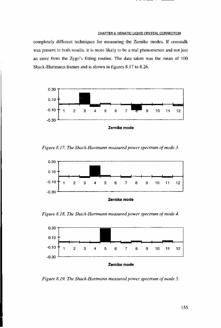
CHAPTER 8: NEMATIC LIQUID CRYSTAL CORRECTION
completely different techniques for measuring the Zernike modes. If crosstalk was present in both results, it is more likely to be a real phenomenon and not just an error from the Zygo's fitting routine. The data taken was the mean of 100 Shack-Hartmann frames and is shown in figures 8.17 to 8.26.
0.30
0.10 -•
0.10" i 2 3 4 5 6 7
Zernike mode
Figure 8.17. The Shack-Hartmann measured power spectrum of mode 3.
0.30
0.10
-0.10
-0.30
--
"* 1 1
2 3 4 5 6 7 8 9 10 11 12
Zernike mode
Figure 8.18. The Shack-Hartmann measured power spectrum of mode 4.
0.30
0.10
-0.10
-0.30
--
" 1 2 3 4 5 6 7 8 9 10 11 12
Zernike mode
Figure 8.19. The Shack-Hartmann measured power spectrum of mode 5.
155
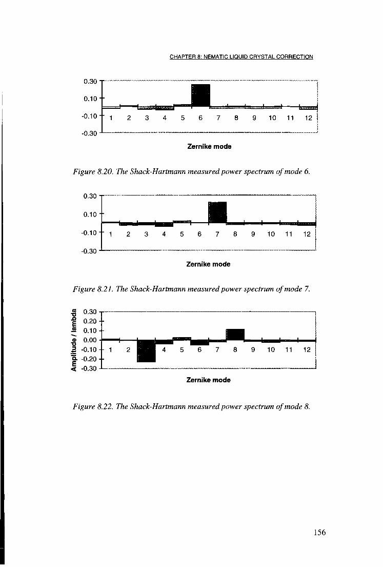
CHAPTER 8: NEMATIC LIQUID CRYSTAL CORRECTION
0.30
0.10
-0.10
-0.30
--1 1 ! 1 J •
"" 1 •
2 3 4 5 6 7 8 9 10 11 12
Zernike mode
Figure 8.20. The Shack-Hartmann measured power spectrum of mode 6.
0.30
0.10
-0.10
-0.30
- • • •• 1 2 3 4 5 6 7 8 9 10 11 12
Zernike mode
Figure 8.21. The Shack-Hartmann measured power spectrum of mode 7.
™ 0.30 | 0.20 i2 0.10--» 0.00 -3 -0.10 |- -0.20 --< -0.30
Zernike mode
Figure 8.22. The Shack-Hartmann measured power spectrum of mode 8.
156
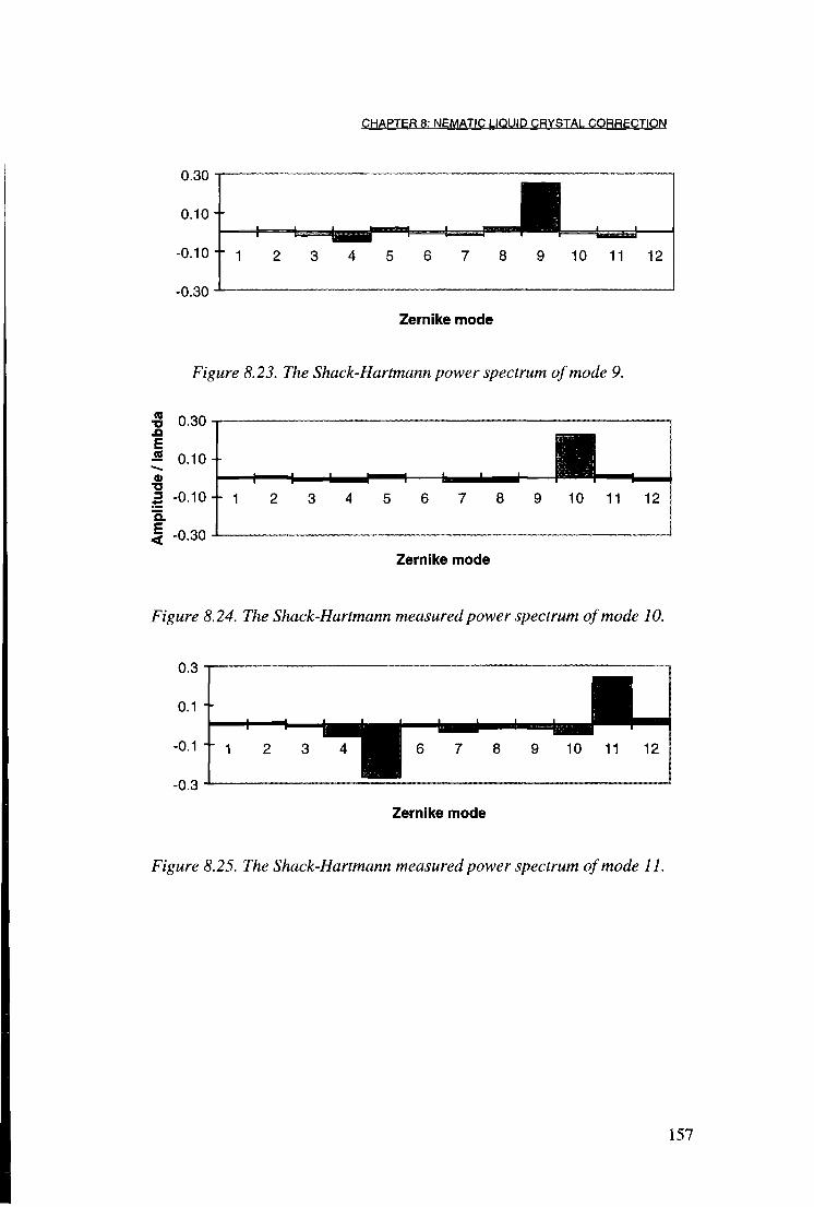
CHAPTER 8: NEMATIC LIQUID CRYSTAL CORRECTION
0.30
-0.30
--1 1
• • 1
1
2 3 4 5 6 7 8 9 10 11 12
Zernike mode
Figure 8.23. The Shack-Hartmann power spectrum of mode 9.
•G 0.30 ji
E
•2 0.10 +
I - ° - 1 0
Q. J -0.30
Zernike mode
10 11 12
Figure 8.24. The Shack-Hartmann measured power spectrum of mode 10.
10 11 12
Zernike mode
Figure 8.25. The Shack-Hartmann measured power spectrum of mode 11.
157

CHAPTER 8: NEMATIC LIQUID CRYSTAL CORRECTION
0.3
i — P « 0.1 ••
-0.3
-0.1 --2 8 10 11 12
-0.5
Zernike mode
Figure 8.26. The Shack-Hartmann measured power spectrum of mode 12.
It can be see from the above figures that the crosstalk between modes was also
present in the Shack-Hartmann measurements. The effect of this crosstalk on the
correction performance will be discussed below.
8.5.4 THE CAUSE OF THE HEX69'S CROSSTALK
The source of the crosstalk in the Hex69 does not come from an electrical source
as in chapter 4, but from the coarse pixelation of the Hex69. It can not reproduce
the complex waveform of the higher order modes. Many of the high order modes
place most of the aberration at the edge of the aperture. Since the pixel size of the
Hex69 is approximately constant over the whole of its aperture, it has more
difficulty reproducing these higher order modes.
The crosstalk can be simulated with a computer model. The DC term of the cross
correlation of two functions gives a measure of the similarity of the two
functions. Unpixelated Zernike modes are orthogonal functions and so there is a
zero DC term of the cross correlation. If f j and fi are two functions, the cross-
correlation is given by
[FT{fx)-FTifjY FT [8.2]
158

CHAPTER 8: NEMATIC LIQUID CRYSTAL CORRECTION
where * represents the complex conjugate and FT is the Fourier transform
function.
Simulations were carried out using MATLAB™. The SLM was represented by
100 10x10 pixels. The first 12 Zernike modes were mapped on to the array and
each was cross correlated with each other. The results are shown in figures 8.27
to 8.38. The lighter shaded bars show the height of the DC term for 100 pixels
and the solid bar is for a 400 pixel SLM.
« = 0.4
5 6 7 8 Zernike Mode
10 11 12
Figure 8.27. Mode 1 cross-correlated with the other Zernike modes.
o .s 0.6
5 6 7 8 Zernike Mode
10 11 12
Figure 8.28. Mode 2 cross-correlated with the other Zernike modes.
159

CHAPTER 8: NEMATIC LIQUID CRYSTAL CORRECTION
g 0.8-j 2 c
o 5 o.6 -I X3 a H> a 0 t 0.4 B ° E o 1 0.2
6 7 8 9 10 11 12 Zernike Mode
Figure 8.29. Mode 3 cross-correlated with the other Zernike modes.
1
0.8 •
0.6 •
0.4
0.2
0 5 6 7 8 9 10 11 12
Zernike Mode
Figure 8.30. Mode 4 cross-correlated with the other Zernike modes.
1
0.8
0.6
0.4 1
0.2
0 5 6 7 8 9 10 11 12
Zernike Mode
Figure 8.31. Mode 5 cross-correlated with the other Zernike modes.
160
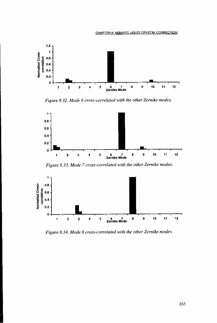
CHAPTER 8: NEMATIC LIQUID CRYSTAL CORRECTION
1.2 n
1 in (A
0.8
to <5
i i i 1 2 3 4 5 6 7 8 9 10 11 12
Zernike Mode
Figure 8.32. Mode 6 cross-correlated with the other Zernike modes.
1
0.8
i i
1 2 3 4 5 6 7 8 9 10 11 12 Zernike Mode
Figure 8.33. Mode 7 cross-correlated with the other Zernike modes.
1
0.8 in at
O in
L i
12 10 11 8 1 Zernike Mode
Figure 8.34. Mode 8 cross-correlated with the other Zernike modes.
161
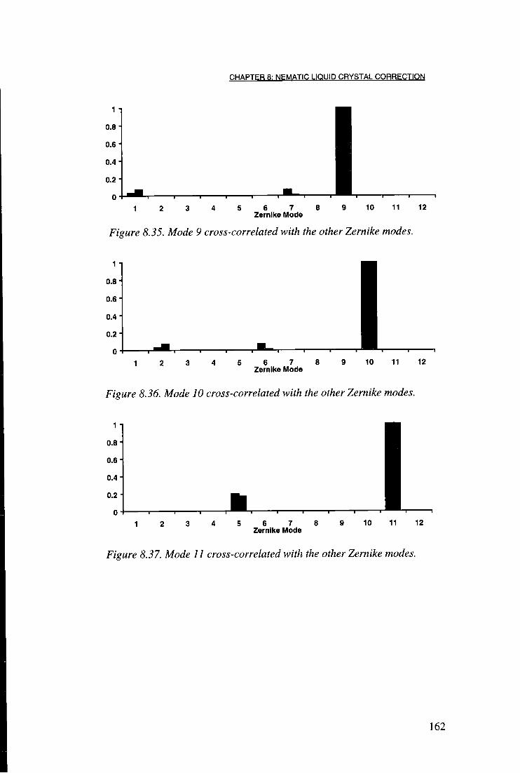
CHAPTER 8: NEMATIC LIQUID CRYSTAL CORRECTION
1 •
0.8-
0.6-
0.4"
0.2-
0 5 6 7 8 9 10 11 12
Zernike Mode
Figure 8.35. Mode 9 cross-correlated with the other Zernike modes.
1
0.8
0.6
0.4 1
0.2
o 5 6 7 8 9 10 11 12
Zernike Mode
Figure 8.36. Mode 10 cross-correlated with the other Zernike modes.
1 n
0.8
0.6
0.4
0.2 1
o 5 6 7 8 9 10 11 12
Zernike Mode
Figure 8.37. Mode 11 cross-correlated with the other Zernike modes.
162
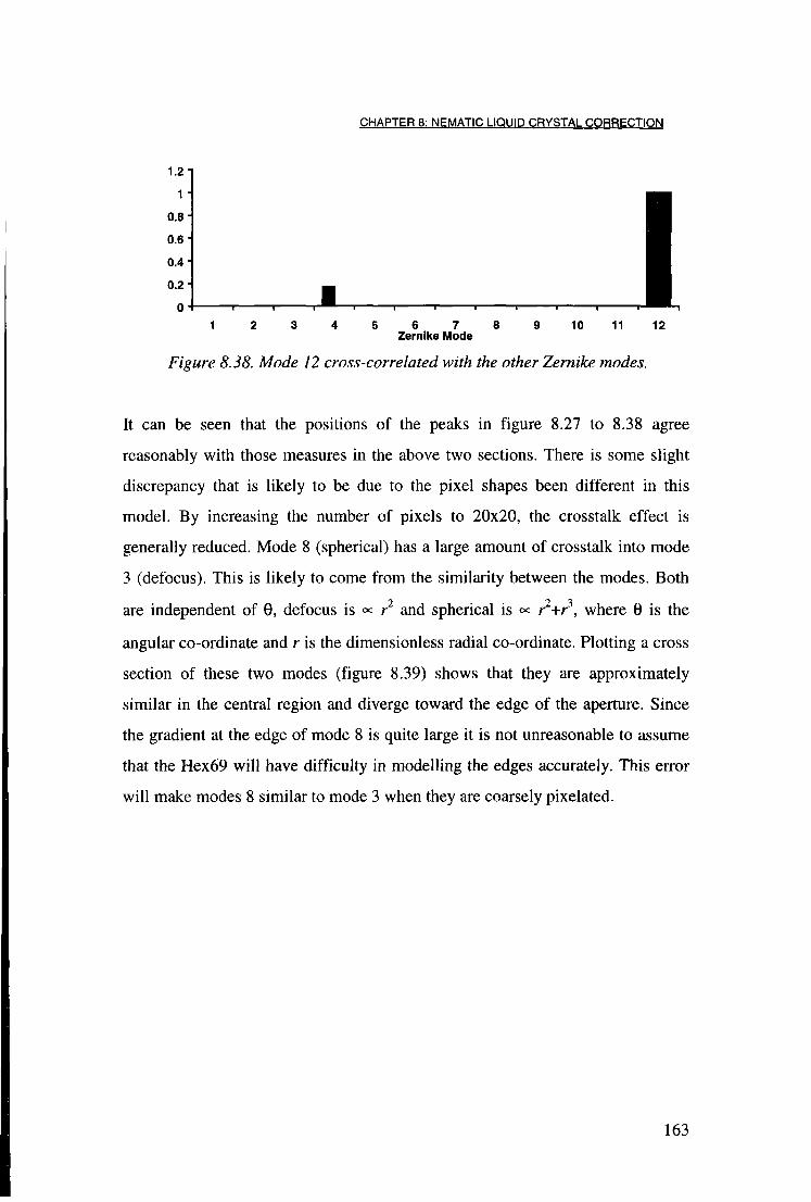
CHAPTER 8: NEMATIC LIQUID CRYSTAL CORRECTION
1 "
0.6-
0.4-
0.2 -1 0
2 3 4 5 6 7 Zernike Mode
8 9 10 11 12
Figure 8.38. Mode 12 cross-correlated with the other Zernike modes.
It can be seen that the positions of the peaks in figure 8.27 to 8.38 agree
reasonably with those measures in the above two sections. There is some slight
discrepancy that is likely to be due to the pixel shapes been different in this
model. By increasing the number of pixels to 20x20, the crosstalk effect is
generally reduced. Mode 8 (spherical) has a large amount of crosstalk into mode
3 (defocus). This is likely to come from the similarity between the modes. Both
are independent of 0, defocus is <*= r2 and spherical is «= r2+r3, where 0 is the
angular co-ordinate and r is the dimensionless radial co-ordinate. Plotting a cross
section of these two modes (figure 8.39) shows that they are approximately
similar in the central region and diverge toward the edge of the aperture. Since
the gradient at the edge of mode 8 is quite large it is not unreasonable to assume
that the Hex69 will have difficulty in modelling the edges accurately. This error
will make modes 8 similar to mode 3 when they are coarsely pixelated.
163

CHAPTER 8: NEMATIC LIQUID CRYSTAL CORRECTION
0
- 1
R a d i u s
Figure 8.39. A cross section of two Zernike modes. One negative wave of defocus
{indicated by stars) and a wave of spherical (solid line) are shown demonstrating
the similarities of the two modes in the central region.
These crosstalk effects can be minimised when the Hex69 is used as the corrector
because of two reasons. The system incorporates negative feedback and so any
added mode will be removed in the next frame. Secondly, the DSP only returns
the first 12 modes to the PC. The low order modes do not generate large amounts
of crosstalk. Out of the 12 modes only the first 8 were used and the amplitude
that could be applied to the Hex69 was limited to ±0.5 waves for each mode.
8.5.5 LABORATORY TURBULENCE SIMULATION
To demonstrate a real time adaptive optics system in the laboratory it is necessary
to introduce randomly varying aberrations, preferably with Kolmogorov statistics.
This was achieved in chapter 6 by using the Hex69 SLM. However, there is
currently only one such device at the University of Durham. An alternative
device was constructed from a cardboard tube about 50cm long with a resistive
wire inside. There was also a computer cooling fan in the centre of the tube to
generate further turbulence. Both of these elements could be controlled by
varying the voltage across them.
164

CHAPTER 8: NEMATIC LIQUID CRYSTAL CORRECTION
0.8 -i
is
w 0.2 c 0.1
1 2 3 4 5 6 7 8 9 10 11 12 Zernike mode
Figure 8.40. The measured RMS Zernike mode amplitudes of the cardboard tube
ATS. The solid bars represent the theoretical modes for a D/ro of 10. The white
bars are the measured modes.
A thousand frames of the Shack-Hartmann were taken to analyse the performance
of the atmospheric turbulence simulator. The RMS of the first 12 Zernike modes
is shown in figure 8.40. Although modes 1 and 2 (tip/tilt) are slightly lower than
desired and mode 4 (astigmatism) is higher, it quantitatively approximates to
Kolmogorov statistics. The lower than average tip/tilt is advantageous because in
a real telescope system there would be a tip/tilt mirror to remove these two terms.
The solid columns in figure 8.40 show the theoretical Kolmogorov power
spectrum for D/ro = 10 (Wang, 1978). Figure 8.41 shows 1000 frames of mode 3
(defocus) measured with the Shack-Hartmann. The temporal characteristics show
abrupt changes in amplitude. This is qualitatively similar to the atmosphere.
165

CHAPTER 8: NEMATIC LIQUID CRYSTAL CORRECTION
0.2
•» 0 CO
V !¥ 0 f
AH 0.
< -0.2
0.3
0.4 0 1
Time/seconds
Figure 8.41. The first 5 seconds of data for mode 3 (defocus).
8.5.6 STATIC CORRECTION
The system was first run with a static aberration added into the optical path. A
piece of aberrating glass was placed in front of the Hex69. The measured modes
were written to a file as the correction was performed. The correction of mode 3
(defocus) is displayed in figure 8.42. It can be seen that it takes 5 frames to
perform a correction from 0.8 waves to system noise level. The frame rate of the
system was 15Hz.
166

CHAPTER 8: NEMATIC LIQUID CRYSTAL CORRECTION
0.8 -•
time/ seconds
Figure 8.42. A step response of mode 3 for a static correction in closed loop.
8.5.7 CLOSED-LOOP EXPECTATIONS
By using equation [7.3] it is possible to estimate the correction achievable with
the Hex69 and Shack-Hartmann system. It can be assumed that the wavefront
sensor noise, OWFS, is the same as before. The temporal bandwidth of the
corrector is taken to be that of the Hex69's electronics frame speed, i.e.,/c=26Hz.
Equation [7.8] requires the wind velocity but this is however unknown for this
simulator. However, by visual inspection, the spots of the Shack-Hartmann
moved at a similar speed to the spots of the Shack-Hartmann used to study the
ATS in chapter 6. To make an order of magnitude calculation of the wavefront
variance the wind velocity has been approximated to 5ms"1, so =0.769
radians2.
The Hex69 is 9 pixels across, and so for D/ro of 10, CTcorr=1.06 radians2, a has
been taken as 1.26 again. The residual error after correcting 8 modes is calculated
from [7.7] and 0 ^ = 2 . 1 4 9 . The total variance is then 3.96 radians2. This is
approximately the same residual variance calculated in §7.3.6 for the FLC.
Despite the Hex69s ability to give analogue correction of the wavefront it is
disadvantaged because of its slower speed contributing to a larger value of cr̂ mp»
167

CHAPTER 8: NEMATIC LIQUID CRYSTAL CORRECTION
and its smaller number of pixels contributing to a larger value of G2
CoTI. However,
the Hex69 does also attempt to correct for a larger D/r0. Using the value of
£)/r0=8.5 which was used in chapter 7, the total residual variance drops to 3.46
radians2. So in theory the system should perform better than the system of chapter
7.
8.5.8 CLOSED LOOP CORRECTION
Closed loop correction was then performed. The system was run with the
simulated turbulence generator. The frame rate of the Shack-Hartmann system
was 40Hz, although the Hex69 was only run at 26Hz. Because of the cross-talk
effects and in an attempt to maximise the speed of the system, only the first 8
modes where used in the correction routine. The PSF measurements were taken
with the ITEX integrating frame grabber, over a period of 10 seconds.
Figure 8.43. Real time correction results. The left graph is the uncorrected PSF,
Strehl ratio = 7%. The right graph is the corrected, Strehl ratio = 12%.
168

CHAPTER 8: NEMATIC LIQUID CRYSTAL CORRECTION
Figure 8.44. The uncorrected PSF (left) and the corrected (right).
Figure 8.43 shows the aberrated and corrected PSFs. These are also shown as an
image in figure 8.44. The Strehl ratio was increase from 7% to 12%, an increase
of a factor of 1.7. The full width half maximum was decreased by a factor of 2.2.
8.5.9 REAL TELESCOPE TRIALS
The above system (without the turbulence simulator) has been tested on a real
telescope. The telescope was the 'Vacuum Tower Telescope' (VTT) at Sunspot,
New Mexico, USA. The telescope has a diameter of 76cm. It was planned to use
the telescopes tip/tilt mirror in conjunction with the Hex69. Unfortunately the
tip/tilt mirror would not work on night-time starlight and the Hex69 had to
correct for tip/tilt itself. Because of the large sweep required in order to correct
tip/tilt, the Hex69 was too slow to correct for the seeing. It is hoped that in the
future the device can be tried again with its own dedicated tip/tilt mirror.
8.6 Discussion
The above experiment shows that correction using the nematic Hex69 is possible.
The improvement in Strehl ratio is non-trivial for a first time system. The
improvement is however lower than the correction achieved in chapter 7. The
Strehl ratio was increased from 7% to 12% (compared with 23% to 33% in
chapter 7). However, as a percentage increase this system gives a larger
improvement (70%, compared to 43% in chapter 7). It is still important to
169

CHAPTER 8: NEMATIC LIQUID CRYSTAL CORRECTION
understand where the losses in performance have occurred and where improvements in future systems can be made.
One of the greatest difficulties with this real time correction was the speed of the
system. This system has not yet been optimised fully. The GAIN„ values for each
mode were set to 0.25 each. With such a low value it was sometimes difficult
tracking the aberrations generated by the ATS. Higher values of GAIN„ were
tried but they tended to cause oscillations in the system. A detailed studied of the
control system is required to optimise the GAIN values.
The cardboard tube method of generating turbulence was not very controllable. It
could not be operated for more than a few minutes before the air flow inside the
tube became settled and no longer produced a large aberration. The speed of the
turbulence is particularly difficult to control. Several lengths of tube were tried
but this had little effect on the controllability of the turbulence. It is well known
that nematic liquid crystal SLMs have slow speeds so it would be desirable to
have more control over the simulated wind speed so that the corrections at
different speeds could be measured.
It has been shown in this chapter that static corrections can be corrected very well
with the Hex69. It can be expected that with a few modifications the system can
be made to perform better. It is not unreasonable to assume that i f the simulated
wind speed could have been reduced, the Hex69 would have improved the Strehl
ratio much more substantially than it did.
The performance should also be improved with the inclusion of a tip/tilt mirror in
the system. In Kolmogorov turbulence, the first two modes have the most power.
This required the SLM to sweep through a larger dynamic range. Since the large
range causes the SLM to slow down considerably, removal of tip/tilt would have
allowed the Hex69 to correct the higher order modes faster. This idea is in line
170

CHAPTER 8: NEMATIC LIQUID CRYSTAL CORRECTION
with other adaptive optics systems such as ELECTRA where a separate mirror removes the tip/tilt.
In conclusion, the system has improved the Strehl ratio of a real time aberration.
Although the increase in the numerical value of the Strehl ratio was smaller than
in the system of the previous chapter, the percentage increase was greater and the
light efficiency of the whole system was considerably higher. A large
improvement in Strehl ratio was demonstrated using the device statically. It is the
author's opinion that i f the speed of the real time system can be increased this
method will provide the best adaptive optics system for astronomical applications
due to it's higher optical transmission and ability to potentially fully correct for
an aberration.
8.7 Summary
In this chapter a nematic liquid crystal adaptive optics system has been built. The
wavefront sensor was a Shack-Hartmann sensor. Cross-talk between various
Zernike modes has been experimentally measured. Both static and real time
corrections have been demonstrated.
The next chapter will draw together the conclusions from all the experimental
chapters and compare the results. It will present the conclusions of this thesis.
171

CHAPTER 9: SUMMARIES AND CONCLUSION
Chapter 9: Summary and Conclusions
9.1 Introduction
The aim of this thesis was to demonstrate working liquid crystal based adaptive
optics systems. This chapter shall begin by summarising the work done in each
of the experimental chapters (chapters 4-8). It will then compare each adaptive
optics system, discussing the merits of each. The final section will discuss
suggestions for future work.
9.2 Summary of Results
9.2.1 CHAPTERS 2 AND 3
Chapters 2 and 3 gave a basic introduction to liquid crystals, atmospheric
turbulence and adaptive optics.
9.2.2 CHAPTER 4
In chapter 4 a multiplexed nematic device was examined. The device was based
on standard display technology, slightly modified to be used as a phase only
modulator.
The device was capable of giving a IX phase shift, however through a series of
experiments to measure the phase shift produced by the device, it was discovered
that there was a large amount of crosstalk between pixels. This crosstalk was
known to happen in intensity modulating multiplexed displays so an experiment
was performed to characterise it. It was found that when half ( A ) of the device
was turned fully on and the other half (B) was turned fully off the actual phases
shifts measured were 5A, on half (B) instead of OA. and 6A. on half ( A ) instead of
the expected IX. By looking at the voltage waveforms it was suggested that this
effect came about from the multiplexing technique.
172

CHAPTER 9: SUMMARIES AND CONCLUSION
Although the crosstalk effects were less severe when only small differences in
the voltages were applied to each half, the device was clearly limited in its
application in adaptive optics. For this reason, no further work was carried out
on the device.
9.2.3 CHAPTER 5
In this chapter, one of the simplest types of adaptive optics to implement was
tested: 'binary adaptive optics'. This system used an FLC SLM with a PDI as
the wavefront sensor. Binary adaptive optics only requires the knowledge of
whether a pixel is in or out of phase. For this reason it is not important to fully
calculate the phase from an interferogram.
A computer model of the system was developed to enable an understanding of
the complexities of the PDI. It was necessary to experiment with several control
algorithms to obtain the best correction performance. An experimental system
was constructed and aberrations were applied. The system corrected from a
Strehl ratio of 5% to 26%. However it took ~5 frames to reach the maximum
correction achievable. Some pixels oscillated. The optical transmission of the
system was also extremely low. Both the FLC and the PDI were very lossy.
9.2.4 CHAPTER 6
In chapter 6 an atmospheric turbulence simulator (ATS) was developed. This
was to test the system in the next chapter. Computer generated phase screens
were produced off line. These were then mapped on to the Meadowlark Hex69
nematic liquid crystal SLM. A Shack-Hartmann wavefront sensor was
constructed to test the performance of the device. The RMS of each Zernike
mode and the Strehl ratio were found to be in reasonable agreement with the
theoretical expectations. The temporal power spectrum showed an expected -8/3
gradient on a log-log graph.
173
CHAPTER 9: SUMMARIES AND CONCLUSION
9.2.5 CHAPTER 7
In chapter 7 the ATS developed in chapter 6 was used as an aberrator in an FLC
binary adaptive optics system. A Displaytech 10x1 Ob FLC SLM was used as the
corrective element and a Shack-Hartmann was the wavefront sensor. The system
was run in real time producing a Strehl ratio improvement from 23% to 33%.
The system ran at a speed of 6Hz. Although the wavefront sensor's light
efficiency was improved, the system was still limited by the lossiness of the FLC
and the low theoretical expectation.
9.2.6 CHAPTER 8
In chapter 8 the FLC was replaced by a Meadowlark Hex69 SLM. This
improved the transmission of the corrective element to 90%. The system was run
in real time with a frame rate of 26Hz. An improvement in Strehl ratio from 7%
to 12% was measured. There was also an analysis of the cross talk between
Zernike modes generated by the Meadowlark. The static correction of a piece of
aberrated glass was also performed. This suggested that i f the device was not so
limited by speed it should be able to correct aberrations very well in a real time
system.
The correction results are summarised in table 9.1. Only considering the Strehl
ratio increase the FLC/PDI system (chapter 5) is considerably better than the
other two. However, the system has a very poor optical transmission. The FLC
only allows 2% of light through and the PDI is known to have low transmission
(although this could be improved by using a phase shifting PDI). The major
problem with this system is its instabilities and the fact it takes several frames to
reach the best solution. These factors make it unsuitable for atmospheric
adaptive optics.
174
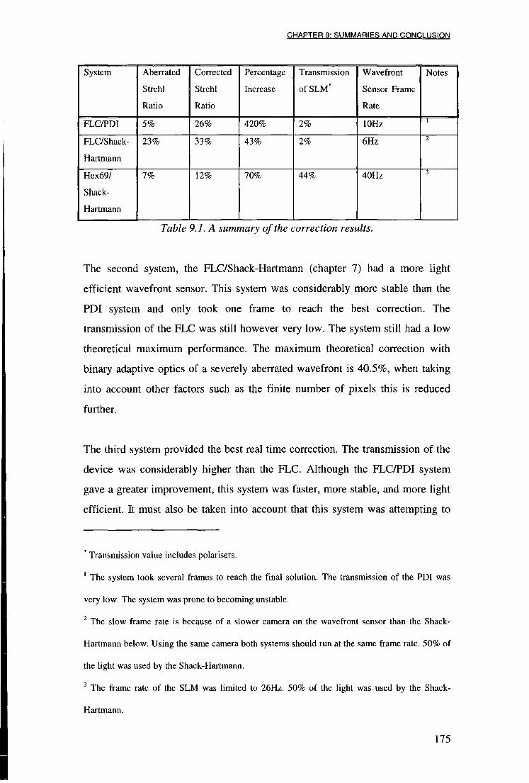
CHAPTER 9: SUMMARIES AND CONCLUSION
System Aberrated
Strehl
Ratio
Corrected
Strehl
Ratio
Percentage
Increase
Transmission
of SLM*
Wavefront
Sensor Frame
Rate
Notes
FLC/PDI 5% 26% 420% 2% 10Hz I
FLC/Shack-
Hartmann
23% 33% 43% 2% 6Hz 2
Hex69/
Shack-
Hartmann
7% 12% 70% 44% 40Hz 3
Table 9.1. A summary of the correction results.
The second system, the FLC/Shack-Hartmann (chapter 7) had a more light
efficient wavefront sensor. This system was considerably more stable than the
PDI system and only took one frame to reach the best correction. The
transmission of the FLC was still however very low. The system still had a low
theoretical maximum performance. The maximum theoretical correction with
binary adaptive optics of a severely aberrated wavefront is 40.5%, when taking
into account other factors such as the finite number of pixels this is reduced
further.
The third system provided the best real time correction. The transmission of the
device was considerably higher than the FLC. Although the FLC/PDI system
gave a greater improvement, this system was faster, more stable, and more light
efficient. It must also be taken into account that this system was attempting to
Transmission value includes polarisers.
1 The system took several frames to reach the final solution. The transmission of the PDI was
very low. The system was prone to becoming unstable.
2 The slow frame rate is because of a slower camera on the wavefront sensor than the Shack-
Hartmann below. Using the same camera both systems should run at the same frame rate. 50% of
the light was used by the Shack-Hartmann.
3 The frame rate of the SLM was limited to 26Hz. 50% of the light was used by the Shack-
Hartmann.
175

CHAPTER 9: SUMMARIES AND CONCLUSION
correct for an aberration greater and faster than that in the FLC/Shack-Hartmann
system. Although the speed of the nematic liquid crystal SLM is slower than the
FLC several options for future work will be discussed later which should make
the device run slightly faster. For this reason, it is the conclusion that the
Meadowlark Hex69 SLM with a Shack-Hartmann wavefront sensor is the best
choice with current technology for a liquid crystal adaptive optics system for
astronomy. Of the three systems tested, this system has filled the criteria required
for an atmospheric adaptive optics system the best.
9.3 Future Work
9.3.1 MEADOWLARK/SHACK-HARTMANN SYSTEMS
One of the most important steps in the next stage of the Meadowlark/ Shack-
Hartmann system would be to increase the speed of the system. Several ideas are
listed below.
1. Improve the drive electronics. At the moment the Meadowlark SLM is been
driven through the printer port. This introduces the 26Hz frame speed. If the
device was driven using a digital interface the bandwidth of the electronics
should improve. Although the speed of the liquid crystal would not increase,
it would mean a faster switching speed for phase shifts <k.
2. Optimisation of the calibration curve. The response time of a nematic liquid
crystal SLM is non-linear, i.e., a shift for 0 to A/2 takes a different amount of
time to a shift from X/2 to 7i. By choosing the correct range to be used by the
calibration curve the liquid crystal will operate slightly faster.
3. Optimisation of the control loop. The control feedback loop for the system
has not been optimised. Analysis of the system using linear control theory
should enable the system gains to be set more accurately allowing the
Meadowlark to reach the desired correction in less frames.
176
CHAPTER 9: SUMMARIES AND CONCLUSION
4. Include a tip/tilt mirror. The largest aberrations in Kolmogorov turbulence are
tip/tilt. These aberrations require the Meadowlark to sweep through a large
range to correct for them. If the tip/tilt was removed with a tip/tilt mirror, the
Meadowlark could be used to only correct the higher order modes. These
modes would require smaller ranges for the liquid crystal and so they could
then be corrected faster.
As well as the above improvements the following should be also done.
1. Optimise the reflectivity of the beam splitter so that as much light as possible
goes to the science camera and the Shack-Hartmann still works.
2. Cascade two devices together. The second device should have its optical axis
orthogonal to the first. There would then be no polariser required and the
transmission should improve to approximately 81% (assuming 90%
transmission for both devices.)
3. A larger number of Zernike modes should be used to control the SLM. This
will improve the total amount of correction possible. Any loss in computer
speed could easily be compensated by replacing the 80486 PC with a Pentium
PC.
9.3.2 FLC/SHACK-HARTMANN S Y S T E M
Currently the FLC system is limited by its poor transmission. Until a high
switching angle device can be developed, PLCs will be of little use in
astronomy. Once high switching angle device are developed PLCs will enable a
very fast adaptive optics system. It will probably be desirable to cascade two or
more devices together to get at least quarter wave switching so that the
aberration can be more fully corrected. The best wavefront sensor for achieving
this wil l probably be the Shack-Hartmann.
177
CHAPTER 9: SUMMARIES AND CONCLUSION
9.3.3 ATMOSPHERIC TURBULENCE SIMULATOR
Many of the improvements that could be made to the Meadowlark adaptive
optics system are applicable to this. In addition, the following is recommended
for further work.
1. If tip/tilt is to be modelled, use a separate tip/tilt mirror to increase the speed
of the liquid crystal.
2. Cascade several devices together to simulate multi-layer turbulence. This
would be useful for testing multi-conjugate adaptive optics systems.
178

APPENDIX 1: THE ZYGO INTERFEROMETER
Appendix 1 : The Zygo Interferometer The Zygo interferometer is used extensively in this thesis. This appendix briefly
describes the device.
A1.1 System Design
The Zygo is a double pass interferometer. The laser source is a lmW red He-Ne. This
light passes through a reference plate that reflects part of the light back to the Zygo's
imaging CCD camera. This is the reference part of the beam. The rest of the light
passes through to the test object. If the test object is transparent, such as a liquid
crystal SLM, an optically flat mirror is placed behind the object. This reflects the light
back into the Zygo where it then interferes with the test beam forming an
interferogram on the CCD camera. A piezo-electrically controlled mirror can alter the
path length of the reference beam so that the (modulo 2K) phase can be completely
calculated. Taking the familiar interference intensity equation
where IQ and al^ are the intensities of the two interfering beams, y is the fringe
contrast (see equation [5.6]) and 0 is the phase between the test and reference beams.
If an additional n/2 phase shift is added to the reference beam (by moving the
reference plate with pizeo-electric crystals) we now get
/ ^ ( l + a ^ o O + ycosCe)) [ A l . l ]
/ 2 = ( l + a 2 > 0 (l-Ysin(e)) [A1.2]
Two additional shifts of the reference beam by n and 3n/2 radians gives
/ 3=(l + a 2) 0(l-ycos(e)) [A1.3]
/ 4 = ( l + a 2 V 0 ( l + ysin(e)) [A1.4]
179

APPENDIX 1: THE ZYGO INTERFEROMETER
From a single measurement it is impossible to determine 9. The arc-cosine does not
give a unique solution, in addition a, y and k are usually unknown. However, i f all
four measurements are made [ A l . l ] , [A1.2], [A1.3], and [A1.4] can be rearranged to
give
6 = arctan f l -I A
4 L2 / , - / , V i
[A1.5]
which does give a unique solution between -K and it radians. I0 and y also cancel. It is
still impossible to distinguish between 0+0 and 27W+9, where n is an integer. The
Zygo gets around this by assuming that the phase is continuous across the aperture,
and adds 2n to any pixels that are discontinuous (over certain threshold) with their
neighbours.
Five measurements are taken by the Zygo. The first four have their reference beams
phase shifted as described above. The fifth is identical to the first and is used to check
for any environmental perturbations that may have occurred during the measurement.
The interferograms are processed off line on an IBM compatible PC.
Al.1.1 T H E Z Y G O PTI SPECIFICATIONS
The Zygo specifications are given in table A l . l . The resolution is determined by the
digitisation of the interferogram by the CCD camera frame grabber. The accuracy is
dependent on the flatness of the optical reference plate. This can be improved by
subtracting the known aberrations of the reference plate from the test data.
180

APPENDIX 1: THE ZYGO INTERFEROMETER
Phase measurement resolution X I 2 5 6
Phase measurement accuracy < A/50 Peak to Valley
Repeatability X I 1 0 0 to l a
Data acquisition time ~ Is
Beam size switchable to 33mm or 102mm
Light source lmW He-Ne Laser, 632.8nm
Table ALL The Zygo interferometer specifications
Al.1.2 Z E R N I K E MODE FITTING
The Zygo fits up to 36 Zernike polynomials to the data. Each term is fitted by
minimising the RMS error from a given test phase screen to typically less than 1/50A,
Any of the Zernike modes can be altered and the measured phase screen regenerated
with the new Zernike modes. This enables tip/tilt to be removed from the data. Tip/tilt
is usually due to a misalignment of the interferometer and so is generally removed.
Al.1.3 DISADVANTAGES OF PHASE SHIFTING I N T E R F E R O M E T E R Y
The obvious disadvantage of this technique of determining phase is that unless four
separate interferometers are used, it is not possible to have a fast data acquisition time.
The Zygo takes about 1 second to take the raw data but about a further minute to post-
process it and write it to disk. This makes real time adaptive optics impossible with
the Zygo.
The other disadvantage is when a pixelated device such as the Meadowlark SLM is
measured, the assumption that the wavefront is smooth and continuous is no longer
valid. If a large aberration is placed on to the Meadowlark SLM, the Zygo software
will not unwrap the phase correctly and the result will be completely different from
the expected phase screen.
181
APPENDIX 1: THE ZYGO INTERFEROMETER
Al.1.4 ADDITIONAL F E A T U R E S
The Zygo can store the data in one of three formats: phase data; 36 fitted Zernike
modes; or raw interferograms. The Zygo software also offers the additional
possibilities: the calculation of point spread and modulation transfer functions;
manipulation of Zernike mode coefficients and phase screens; and various data display
options.
182

APPENDIX 2: THE DESIGN OF A NON-PIXELATED SLM
Appendix 2: The design of a non-pixeiated SLM One of the limits of adaptive optics systems is the limited number of actuators that
perform the correction. With deformable mirrors this can be limited by the cost and
the technical demands of constructing such a large number of actuators. In liquid
crystal SLMs the limit comes from the large number of connections requiring either a
large dead space between pixels or having to multiplex and so losing accuracy. In this
appendix a novel liquid crystal alternative is proposed. The device has no pixels to
speak of, but is more like a continuous face plate deformable mirror. There is also the
possibility of a very large number of actuators. With 0.5p.m wide electrodes it should
be possible to achieve an actuator density of ~2*104 per cm2. This would have no
problems of interpixel dead space, although this calculation does not address the
problem of how to electrically connect such a large number of electrodes.
A2.1 Basic design
The basic idea is to use a resistive layer instead of individual pixels. Starting from the
top layer there would be
1. A layer of ITO 1 coated glass. This would be the electrical ground.
2. Nematic liquid crystal material, with parallel alignment.
3. An electrically resistive material such as silicon. To this there would be electrodes
attached at discrete points.
Because the electrodes are connected by a resistive layer there will be a ramp function
in the voltage from an electrode with a high voltage applied and an electrode with a
lower voltage (see figure A2.1)
1 ITO (or indium tin oxide) is a transparent electrical conducting layer deposited on glass and is used
for liquid crystal applications.
183
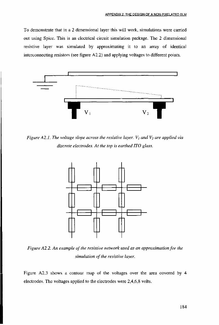
APPENDIX 2: THE DESIGN OF A NON-PIXELATED SLM
To demonstrate that in a 2 dimensional layer this will work, simulations were carried
out using Spice. This is an electrical circuit simulation package. The 2 dimensional
resistive layer was simulated by approximating it to an array of identical
interconnecting resistors (see figure A2.2) and applying voltages to different points.
. I 1
^ ^ " v ^ V 2
Figure A2.1. The voltage slope across the resistive layer. Vi and \ 2 are applied via
discrete electrodes. At the top is earthed ITO glass.
}
Figure A2.2. An example of the resistive network used as an approximation for the
simulation of the resistive layer.
Figure A2.3 shows a contour map of the voltages over the area covered by 4
electrodes. The voltages applied to the electrodes were 2,4,6,8 volts.
184
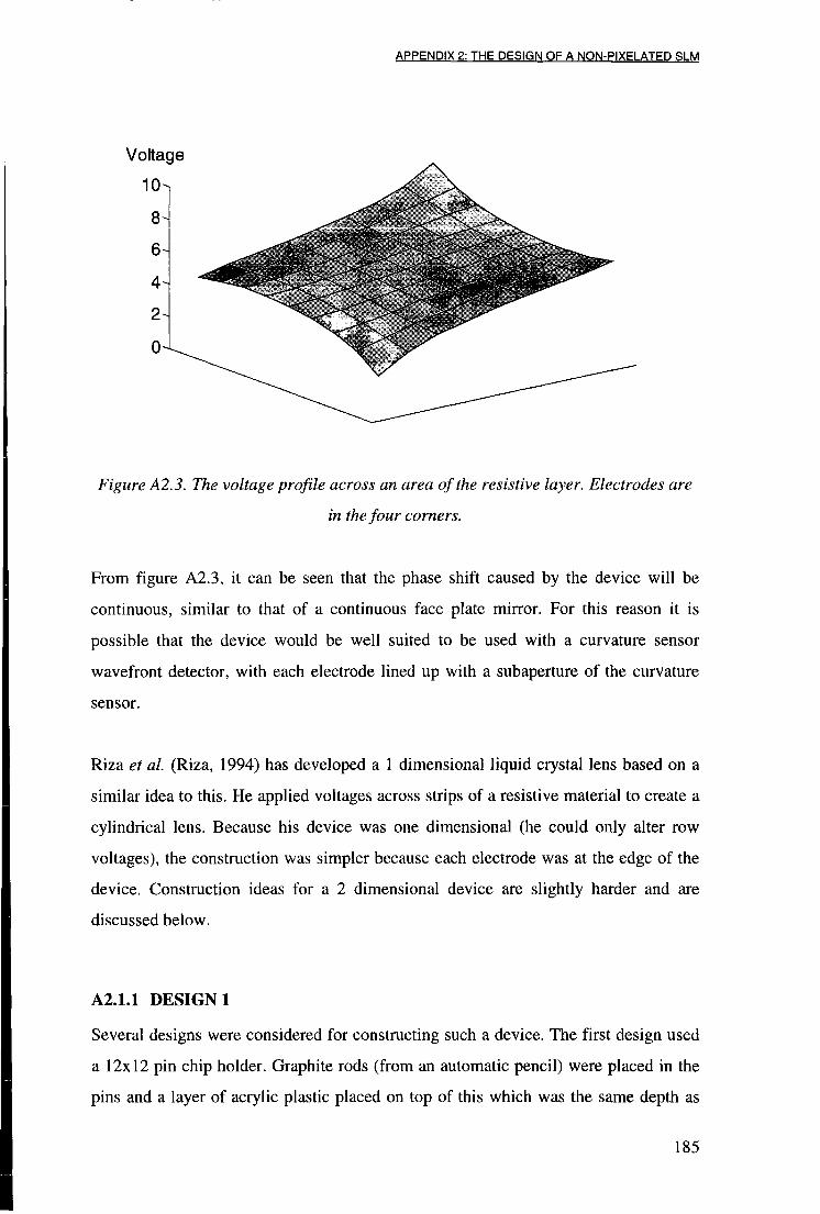
APPENDIX 2: THE DESIGN OF A NON-PIXELATED SLM
Voltage
10
8
x -
0
Figure A2.3. The voltage profile across an area of the resistive layer. Electrodes are
in the four corners.
From figure A2.3, it can be seen that the phase shift caused by the device will be
continuous, similar to that of a continuous face plate mirror. For this reason it is
possible that the device would be well suited to be used with a curvature sensor
wavefront detector, with each electrode lined up with a subaperture of the curvature
sensor.
Riza et al. (Riza, 1994) has developed a 1 dimensional liquid crystal lens based on a
similar idea to this. He applied voltages across strips of a resistive material to create a
cylindrical lens. Because his device was one dimensional (he could only alter row
voltages), the construction was simpler because each electrode was at the edge of the
device. Construction ideas for a 2 dimensional device are slightly harder and are
discussed below.
A2.1.1 DESIGN 1
Several designs were considered for constructing such a device. The first design used
a 12x12 pin chip holder. Graphite rods (from an automatic pencil) were placed in the
pins and a layer of acrylic plastic placed on top of this which was the same depth as
185

APPENDIX 2: THE DESIGN OF A NON-PIXELATED SLM
the graphite rods. The surface of the device was then polished to get it optically flat. A
resistive layer was then to be deposited on top of this (see figure A2.4). The exact
material to be used was to be determined. Options included depositing a
semiconductor on top or painting a layer of conducting glue on and re-polishing.
LC
Resitive layer
Graphite rods
Chip holder
ITO glass
m i l i u m 111 ill y u u u u u u u u u u
^ — Metal pins
«- Acrylic
Figure A2.4. The first design.
Surface Profile / waves 10
Figure A2.5. A surface profile of the plastic layer measured with the Zygo
interferometer.
186
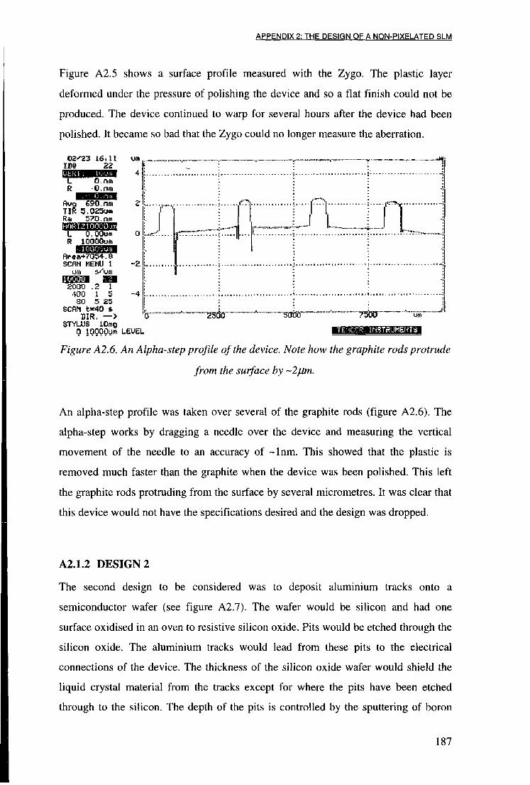
APPENDIX 2: THE DESIGN OF A NON-PIXELATED SLM
Figure A2.5 shows a surface profile measured with the Zygo. The plastic layer
deformed under the pressure of polishing the device and so a flat finish could not be
produced. The device continued to warp for several hours after the device had been
polished. It became so bad that the Zygo could no longer measure the aberration.
02-^3 16: 11 im 22 L R •O.nm
ftvg 690.m TIR 5.025y«i Ra 570. rim HOfi12100001
L R
0,OOum iOQOOum
..IGOnijum
SCAN MENU 1
urn
-2
£000 .2 1 400 1 5 80 5 25
SCAN t«40 & DIR. — >
STYLUS lOmg o looooutt LeyEL
> l < t k ^ l H ' l r ' < l l l " 1 t - - j
2500"" "'HOOD'" • •TSO'fJ'-'
TEMGOR: :INSTrlUMEHTi
Figure A2.6. An Alpha-step profile of the device. Note how the graphite rods protrude
from the surface by ~2jdm.
An alpha-step profile was taken over several of the graphite rods (figure A2.6). The
alpha-step works by dragging a needle over the device and measuring the vertical
movement of the needle to an accuracy of ~lnm. This showed that the plastic is
removed much faster than the graphite when the device was been polished. This left
the graphite rods protruding from the surface by several micrometres. It was clear that
this device would not have the specifications desired and the design was dropped.
A2.1.2 DESIGN 2
The second design to be considered was to deposit aluminium tracks onto a
semiconductor wafer (see figure A2.7). The wafer would be silicon and had one
surface oxidised in an oven to resistive silicon oxide. Pits would be etched through the
silicon oxide. The aluminium tracks would lead from these pits to the electrical
connections of the device. The thickness of the silicon oxide wafer would shield the
liquid crystal material from the tracks except for where the pits have been etched
through to the silicon. The depth of the pits is controlled by the sputtering of boron
187

APPENDIX 2: THE DESIGN OF A NON-PIXELATED SLM
ions onto the reverse surface of the silicon. When the etching acid reaches the boron,
it stops. This design has promise but the device was deemed to be too fragile to
withstand the rest of the construction process (Wood, 1996).
Si layer
SO
- Al electrode
Figure A2.7. Design 2. The liquid crystal material would go on top of the Si layer.
The Si02 would shield the liquid crystal from the Al electrodes except at the points
were pits are etched.
A2.1.3 DESIGN 3
The final design was the most promising. The device would be built on a glass
substrate. This gives a strong, hard and optically flat surface. The aluminium electrode
tracks are then deposited on to the glass lithographically. On top of this, a layer of
silicon oxide (or liquid glass) is deposited. Holes are then etched into the layer
through to the aluminium tracks (with an acid that does not readily attack aluminium),
and a layer of semiconductor (silicon) is deposited on top of this. The rest of the cell
can be constructed on top of this, i.e., the liquid crystal layer and ITO glass (see figure
A2.8).
188
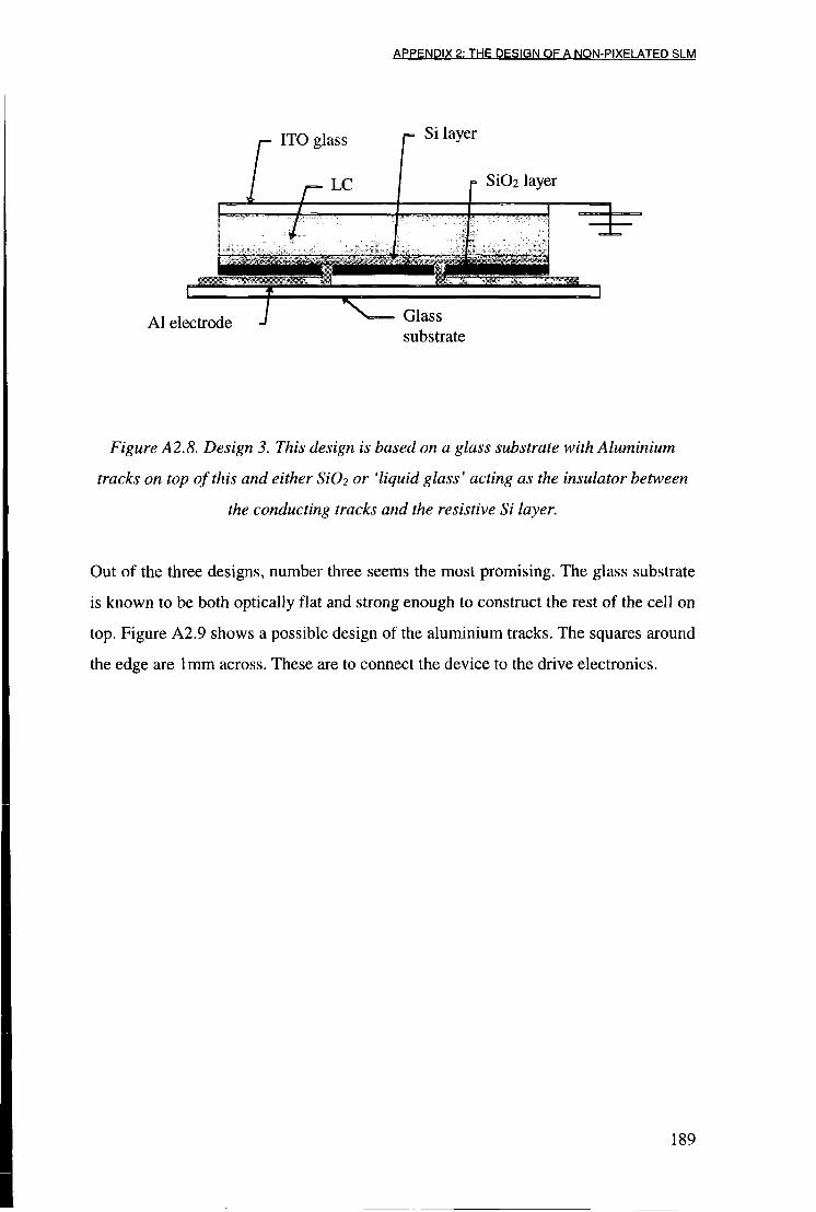
APPENDIX 2: THE DESIGN OF A NON-PIXELATED SLM
Si layer ITO glass
L S1O2 layer LC
f 9MS
an
1 Glass Al electrode substrate
Figure A2.8. Design 3. This design is based on a glass substrate with Aluminium
tracks on top of this and either Si(?2 or 'liquid glass' acting as the insulator between
the conducting tracks and the resistive Si layer.
Out of the three designs, number three seems the most promising. The glass substrate
is known to be both optically flat and strong enough to construct the rest of the cell on
top. Figure A2.9 shows a possible design of the aluminium tracks. The squares around
the edge are 1mm across. These are to connect the device to the drive electronics.
189

APPENDIX 2: THE DESIGN OF A NON-PIXELATED SLM
Figure A2.9. A possible design for the electrode tracks. The central square area
would be the active area. The diagonal tracks connect this to the pads around the
edge. This is so that wires can be connected to the device.
A2.2 Summary
In this appendix, an idea for a liquid crystal device with no pixels and the potential for
a very large number of degrees of freedom has been described. Three methods of
constructing such a device have been described. The actual construction of such a
device is outside the realms of this thesis, but such a device will hopefully be built in
the future.
190
REFERENCES
References
Anderson, 1995
AOA
Amako, 1993
Babcock, 1953
Beckers, 1993
Biernacki, 1991
Bold, 1997
Bonaccini, 1991
Broomfield,
1995a
Broomfield,
1995b
C. S. Anderson, "Fringe visibility, irradiance, and accuracy in
common path interferometers for visualization of phase
disturbances."^/?. Opt. 34 (32) pp 7474-7485 (1995)
Adaptive Optics Associates, Inc. 54 Cambridge Park Drive.
Cambridge, MA 02140-2308. USA
J. Amako, H. Miura, T. Sonehara, "Wave-front control using
liquid crystal devices." Appl. Opt. 32 (23) pp 4323-4329
(1993)
H. W. Babcock, Publ. Astron. Soc. Pac. 65 (1953)
J. M. Beckers, "Adaptive optics for astronomy: Principles,
performance, and applications." Annu. Rev. Astron. Astrophys.
31 pp 13-62(1993)
P. Biernacki, T Brown, M Freeman, "Polarisation dependence
and uniformity of FLC layers for phase modulation." SPIE
Liquid Crystal Devices and Materials 1455 pp 167-178 (1991)
G. T. Bold, T. H. Barnes, J. Gourlay, R. M . Sharpies, T. G.
Haskell, "Practical issues for the use of liquid crystal spatial
light modulators in adaptive optics." Opt. Comms. In print.
D. Bonaccini, G. Brusa, S. Esposito, P. Salinari, P. Stefanini,
V. Biliotti, "Adaptive optics wavefront correction using
addressable liquid crystal retarders." Proc. Soc. Photo-Opt.
Instrum. Eng. 1543 (1991)
S. E. Broomfield, M. A. A. Neil, E. G. S. Paige, I . O. Thomas,
"Binary optical correction of a wavefront aberration using
spatial light modulators." Proc. Soc. Photo-Opt. Eng. 2534,
167-175 (1995)
S. E. Broomfield, M . A. A. Neil, E. G. S. Paige,
"Programmable multiple level phase modulation that uses
ferroelectric liquid crystal spatial light modulators." App. Opt.
34 (29) pp 6652-6665 (1995)
191

REFERENCES
Buffington, 1976
Buffington, 1977
Buscher, 1997
Cao, 1994
Conan, 1995
Clark, 1994
Displaytech
Doel, 1990
Dou, 1995
Efron, 1985
Fogel, 1994
A. Buffington, F. S. Crawford, R. A. Miller, C. D. Orth, "First
observatory results with an image sharpening telescope.'' J.
Opt. Soc. Am. 67 (3) pp 304-305 (1976)
A. Buffington, F. S. Crawford, R. A. Miller, A. J. Schwemin,
R. G. Smits, "Correction of a atmospheric distortion with an
image-sharpening telescope." J. Opt. Soc. Am. 67 (3) pp 298-
303 (1977)
D. F. Buscher, A. P. Doel, C. N. Dunlop, R. M . Myers, D. J.
Robertson, R. M. Sharpies, A. J. Vick, A. Zadrozny, "First
results from the ELECTRA adaptive optics system." Proc.
Soc. Photo-Opt. lustrum. Eng. 3126 (1997) In press.
G. Cao, X Yu. "Accuracy analysis of a Hartmann-Shack
wavefront sensor operated with a faint object." Opt. Eng. 33
(7) pp 2331-2335 (1994)
J. Conan, "Wave-front temporal spectra in high resolution
imaging through turbulence." J. Opt. Soc. Am. A 12 pp 1559-
1570
M . G. Clark "Current status and future prospects of poly-Si
devices." IEE Proc.-Circuits Devices Syst. 141 (1) pp 3-8
(1994)
Displaytech, Inc. 2602 Clover Basin Drive. Longmont, CO
80503. USA
A. P. Doel, C. N. Dunlop, J. V. Major, R. M . Myers, A.
Purvis, M. G. Thompson, "Stellar image stabilisation using
piezo-driven active mirrors." In L D Barr, editor, Advanced
Technology Optical Telescopes IV, SPIE pp 179 (1990)
R. Dou, M . K. Giles, "Closed-loop adaptive optics system
with a liquid crystal television as a phase retarder." Opt. Lett.
20, 1583-1585 (1995)
U. Efron, "The Silicon Liquid Crystal Light Valve." J. Appl.
Phys. 57 (4) pp 1356-1368 (1985)
D. B. Fogel, "An Introduction to Simulated Evolutionary
192
REFERENCES
Foy, 1985
Freeman, 1992
Fried, 1965a
Fried, 1965b
Glindemann,
1993
Greenwood, 1977
Hardy, 1977
Hitachi, 1991
Hudgin, 1977
Hufnagel, 1974
Johnson, 1990
Optimisation." IEEE Transactions on Neural Networks 5(1)
pp3-13(1994)
R. Foy, A. Labeyrie, "Feasibility of adaptive telescope with
laser probe." Astron. Astrophys. 152, (2) pp L29-L31 (1985)
M . O. Freeman, T. A. Brown, D. M . Walba, "Quantized
complex ferroelectric liquid crystal spatial light modulators."
Appl. Opt. 31 (20), pp 3917-3929 (1992)
D. L. Fried, "The Effect of Wave-front Distortion on the
Performance of an Ideal Optical Heterodyne Receiver and
Ideal Camera." Conf. on Atmospheric Limitations to Optical
Propagation, US. Nat. Bur. Stds. CRPL. (1965)
D. L. Fried, "Statistics of a Geometric Representation of
Wavefront Distortion." J. Opt. Soc. Am. 55 (11) pp 1427
(1965)
A. Glindemann, R. G. Lane, J. C. Dainty, "Simulation of time-
evolving speckle patterns using Kolmogorov statistics."
Journal of Modern Optics 40 (12) pp 2381-2288 (1993)
D. P. Greenwood, "Bandwidth specifications for adaptive
optics systems." J. Opt. Soc. Am. 67 pp 390-392 (1976)
J. W. Hardy, J. E. Lefebvre, C. L. Koliopoulos, "Real-time
atmospheric compensation." J. Opt. Soc. Am. 67 (3) pp 360-
369 (1977)
Hitachi, "Hitachi LCD Controller/Driver LSI.", 5 t h edition,
Hitachi Ltd, Japan, 1991
R. Hudgin, "Wave-front compensation error due to finite
corrector-element size." J. Opt. Soc. Am. 67 (3) pp 393-395
R. E. Hufnagel, Proc. Topical Mtg. on Opt. Propagation
through Turbulence, Boulder, CO (1974)
K. M . Johnson, C.C. Mao, G. Moddel, M. A. Handschy, K.
Arnett "High-speed, low power optical phase conjugation
using a hybrid amorphous silicon/ferroelectric-liquid-crystal
device." Opt. Letts. 15 (20) pp 1114-1116 (1990)
193

REFERENCES
Johnson, 1993
Kadono, 1994
Kim, 1988
Kolmogorov,
1961
Kuo, 1994
Kwon, 1984
Landereth, 1992
Lane, 1992
Liu, 1993
Love, 1993
Love, 1994
K. M . Johnson, D. J. McKnight, I Underwood "Smart Spatial
Light Modulators Using Liquid Crystal On Silicon," IEEE
Journal of Quantum Electronics 29 (2) pp 699-714 (1993)
H. Kadono, M . Ogusu, S. Toyooka, "Phase shifting common
path interferometer using a liquid crystal phase modulator."
Opt. Comms. 110 pp 39-400 (1994)
H. M . Kim, J. W. Jeong, M . H. Kang, S. I . Jeong, "Phase
correction of a spatial light modulator displaying a binary
phase-only filter" Appl. Opt. 27(20),4167-4168 (1988)
A. Kolmogorov, "Turbulence - Classic Papers in Statistical
Theory." Interscience Publishers Inc. New York (1961)
C. Kuo, "Optical tests of an intelligently deformable mirror
for space telescope technology." Opt. Eng. 33 (3) pp 791-799
(1994)
O. Y. Kwon, "Multichannel phase shifted interferometer."
Opt. Letts. 9 pp 59-61 (1984)
B. Landreth, G. Moddel, "Gray scale response from optically
addressed spatial light modulators incorporating surface-
stabilized ferroelectric liquid crystals." App. Opt. 31 (20) pp
3937-3943 (1992)
R. G. Lane, A. Glindemann, J. C. Dainty, "Simulation of a
Kolmogorov phase screen." Waves in random media 2 pp
209-224(1992)
J. Liu, K. M. Johnson, M. G. Robinson, "Room temperature
10MHz electro-optical modulation in ferroelectric liquid
crystals." Appl. Phys. Letts. 62 (9) pp 934-936 (1993)
G. D. Love, R. Myers, A. Purvis, R. Sharpies, A. Glindemann,
"A new approach to adaptive wavefront correction using a
liquid crystal half wave phase shifter." ICO-16 Conference on
Active and Adaptive Optics, European Southern Observatory,
Garching, Germany (1993)
G. D. Love, S. R. Restaino, G. C. Loos, A. Purvis, "Wavefront
194

REFERENCES
control using a 64x64 pixel liquid crystal array." Proc. Soc.
Photo-Opt. Instrum. Eng. 2201 pp 1068-1072 (1994)
Love, 1995 G. D. Love, N. Andrews, P. M. Birch, D. Buscher, C. Dunlop,
J. Major, R. Myers, A. Purvis, R. Sharpies, A. Vick, A.
Zadrozny, S. R. Restaino, A. Glindemann, "Binary adaptive
optics: atmospheric correction with a half-wave phase shifter."
App. Opt. 34 (27) pp 6058-6066 (1995) & Addendum 35 (3)
pp 347-350(1996)
Love, 1996 G. D. Love, J. Gourlay, "Intensity-only modulation for
atmospheric scintillation correction by liquid crystal spatial
light modulators." Opt. Letts. 21 (18) pp 1496-1498 (1996)
Love, 1997 G. D. Love, "Wave-front correction and production of Zernike
modes with a liquid crystal spatial light modulator." Opt. Soc.
Am. 36 (7) pp 1517-1524 (1997)
Mercer, 1996 C. R. Mercer, K Creath, "Liquid crystal point diffraction
interferometer for wavefront measurements." App. Opt. 35
(10) pp 1633-1642(1996)
Moddel, 1987 G. Moddel, K. M . Johnson, M . A. Handschy,
"Photoaddressing of High Speed Liquid Crystal Spatial Light
Modulators." Soc. Photo. Instr. Eng. 754 pp 207-213 (1987)
Muller, 1974 R. A. Muller, A. Buffington, "Real-time correction of
atmospheric degraded telescope images through image
sharpening." 64 (9) pp 1200-1210 (1974)
Neil, 1994 M. A. A. Neil, E. G. S. Paige, "Improved transmission in a
two-level, phase only, spatial light modulator." Elec. Letts. 30
(5) pp 445-446 (1994)
Newton, 1704 I . Newton, "Opticks." Dover Publications, Inc. New York
(1979 Edition) ppll0(1704)
Noll, 1976 R. J. Noll, "Zernike polynomials and atmospheric turbulence."
J. Opt. Soc. Am. 66 (3) pp 207-211 (1976)
O'Meara, 1976 T. R. O'Meara, "The multidither principle in adaptive optics."
J. Opt. Soc. Am. 67 (3) pp 306-315 (1976)
195
REFERENCES
Pankove, 1980
Purvis , 1993
Rigaut, 1991
Riza, 1994
Roddier, 1990
Rousset, 1990
Schroeder, 1987
Smartt, 1975
Smartt, 1979
Spektor, 1995
Srinivas, 1994
J. J. Pankove, "Topics in applied physics: Display Devices."
Spinger-Verlag, Berlin 1980
A Purvis, N. J. Bailey, G. D. Love J. V. Major, "Optical
design, simulation and testing of an addressable 64x64 liquid
crystal phase plate." Proc. Soc. Photo. Opt. Instrum. Eng.
2000, pp 96-100(1993)
F. Rigaut, G. Rousset, P. Kern, J. C. Fontanella, J. P. Gaffard,
F. Merkle, P. Lena, "Adaptive optics on a 3.6-m telescope:
results and performance." Astron. Astrophys. 250 pp280-290
(1991)
N. A. Riza, M. C. DeJule, "A novel programmable liquid
crystal lens device for adaptive optical interconnect and
beamforming applications." Opt. Comput. Int. Conf. pp 231-
234 (1994)
N. Roddier, "Atmospheric wavefront simulation using zernike
polynomials." Opt. Eng. 29 (10) pp 1174-1180 (1990)
G. Rousset, J. C. Fontanella, P. Kern, P. Gigan, F. Rigaut, P.
Lena, C. Boyer, P. Jagourel, J. P. Gaffard, F. Merkle, "First
diffraction-limited astronomical images with adaptive optics."
Astron. Astrophys. 230 pp L29-L32 (1990)
D. J. Schroeder, "Astronomical Optics." Academic Press Inc.
San Diego (1987) pp319
R N Smartt, W H Steel. "Theory and Application of Point-
Diffraction Interferometers." Japan J. Appl. Phys. 14 (1975)
Suppl. 14-1
R. N. Smartt, "Special applications of the point diffraction
interferometer." Proc. Soc. Photo Opt Instrum 193 pp 35-40
(1979)
B. Spektor, J. Shamir, "Wave-front analysis using Fresnel lens
array." Opt. Letts. 20 (13) pp 1504-1506 (1995)
M . Srinivas, L. M. Patnaik, "Genetic Algorithms: A Survey."
Computer 27 (6) pp 17-26 (1994)
196
REFERENCES
Tarn, 1990
Thomas, 1993
Tyson, 1991
Ulrich, 1988
Wang, 1978
Warr, 1995
Wood, 1996
Worboys, 1993
Yoshikawa, 1997
E C Tarn, S Wu, A Tanone, F T S Yu, D A Gregory. "Closed-
loop binary phase correction of an LCTV using a point
diffraction interferometer." IEEE Phot. Tech. Letts. 2(2), 143-
146(1990)
I . Thomas, "Programmable correction for optical aberrations
using a phase-only spatial light modulator." MSc degree at the
Department of Engineering Science. University of Oxford,
UK. (1993)
R. Tyson, "Principles of Adaptive Optics." Academic Press
London (1991)
P. B. Ulrich, "Hufnagel-Valley profiles for specified values of
the coherence length and isoplanatic patch angle." W. J
Schafer Associates, WJSA/MA/TN-88-013 (1988)
J. Wang, J. K. Markey, "Modal compensation of atmospheric
turbulence phase distortion." J. Opt. Soc. Am. 68(1) pp 78-87
(1978)
S. T. Warr, R. J. Mears , "Polarisation insensitive operation of
ferroelectric liquid crystal devices." Elec. Letts. 31 (9) pp 714-
716(1995)
D. Wood, University of Durham. Private communication.
(1996)
M. R. Worboys, G. White, K. Mitchell, A. Mosley "Miniature
Display Technologies for Integrated Helmet Systems." GEC
Journal of Research 10 2 pp 111-118 (1993)
N. Yoshikawa, M. Itoh, T. Yatagai "Adaptive Computer-
Generated Hologram Using Interpolation Method." Optical
Review 4 (IB) pp 161-163 (1997)
197