Progress In Electromagnetics Research B, Vol. 60, 301–315, 2014

Ducting and Turbulence Effects on Radio-Wave Propagationin an Atmospheric Boundary Layer

Yung-Hsiang Chou and Jean-Fu Kiang*

Abstract—The split-step Fourier (SSF) algorithm is applied to simulate the propagation of radiowaves in an atmospheric duct. The refractive-index fluctuation in the ducts is assumed to follow a two-dimensional Kolmogorov power spectrum, which is derived from its three-dimensional counterpart viathe Wiener-Khinchin theorem. The measured profiles of temperature, humidity and wind speed in theGulf area on April 28, 1996, are used to derive the average refractive index and the scaling parameters inorder to estimate the outer scale and the structure constant of turbulence in the atmospheric boundarylayer (ABL). Simulation results show significant turbulence effects above sea in daytime, under stableconditions, which are attributed to the presence of atmospheric ducts. Weak turbulence effects areobserved over lands in daytime, under unstable conditions, in which the high surface temperatureprevents the formation of ducts.

1. INTRODUCTION

There are three basic types of atmospheric duct: Surface duct, surface-based duct and elevated duct.A surface duct is usually caused by a temperature inversion [1]. An evaporation duct is a specialcase of surface duct, which appears over water bodies accompanied by a rapid decrease of humiditywith altitude [2]. Surface-based ducts are formed when the upper air is exceptionally warm and drycompared with that on the surface [2]. Elevated ducts usually appear in the trade-wind regions betweenthe mid-ocean high-pressure cells and the equator [2].

Non-standard tropospheric refraction may create a ducting, which can bend the surface-based radarbeams from the anticipated direction [3]. Ducting may also affect radio communications links [4, 5], orfalsely extend the apparent radar range of a target on or near the sea surface [2].

Ducts are frequently observed in the coastal areas where the horizontal variation of refractive-indexcan not be ignored. In [6], a range-independent surface-based duct has been compared with a mixedland-sea path, using two M -profiles.

In these ducting environments, the wave equation can be approximated by a parabolic equation(PE), which can then be solved using numerical techniques like the split-step Fourier (SSF) [7], finitedifference [8], or finite element algorithm [9]. The SSF algorithm is numerically stable and allows alarger step size in the propagation direction, making it suitable to compute the field distribution overlong ranges. The PE model appears to provide a fair estimation of path-related parameters over a widerange of frequencies (X, Ka and W bands) and a variety of atmospheric conditions [10].

Turbulent motions in an atmospheric boundary layer (ABL) are driven primarily by the wind shearin the layer and the solar heating on the bottom surface [11]. The effects of air turbulence has beenstudied by applying a perturbation technique in a mode theory [12], or applying a phase-screen methodin an SSF model [13, 14]. The results of different models have been compared over a series of over-water

Received 22 June 2014, Accepted 21 August 2014, Scheduled 26 August 2014* Corresponding author: Jean-Fu Kiang (jfkiang@ntu.edu.tw).The authors are with the Department of Electrical Engineering, Graduate Institute of Communication Engineering, National TaiwanUniversity, Taipei 106, Taiwan, R.O.C..

302 Chou and Kiang

measurements, in a nearly standard atmosphere [14]. When the turbulence effect is included in themodel, matching with the measured data has always been improved, especially at higher frequencies.

By including rough sea surface, the modeled data become closer to the measured data [15]; butthe path-loss is still underestimated by 3 to 12 dB, partly attributed to the turbulence. Monte-Carlosimulations have been used to study the scattering properties of scalar waves in randomly fluctuatingslabs with an exponential spatial correlation, as well as non-exponential spatial correlations [16, 17].

The scaling approach is often used to describe the turbulence in an atmospheric boundary layer(ABL), which is divided into various regions, with each characterized by different scaling parameters.Thus, the structure of an ABL can be described in terms of only a few characteristic parameters. Thevalidity of the scaling approach has been confirmed by experiments and by numerical simulations, underunstable and stable ABL [18–21].

In this work, the SSF algorithm is applied to simulate the wave propagation over a long horizontalrange. Monte-Carlo simulations are used to generate profiles of refractive-index fluctuation in theatmosphere, and the scaling approach is used to model the structure of the ABL. The relevant modelsare described in Section 2, the proper ranges of parameters involved in these models are evaluated inSection 3, simulation results of practical atmospheric ducts are presented and discussed in Section 4.Finally, some conclusions are drawn in Section 5.

2. CONSTRUCTION OF MODELS

2.1. Propagation Model

Under the paraxial approximation that the wave predominantly propagates in the horizontal (x)direction, the Helmholtz wave equation reduces to the parabolic equation [7]

∂u(x, z)∂x

� j

{k

2[m2(x, z) − 1

]+

12k

∂2

∂z2

}u(x, z) (1)

where x is the propagation range, z the height above the Earth surface, k the wavenumber in freespace, m = 1 + M × 10−6, and the modified refractivity M is related to the refractivity N asM = N + 0.157z. Eq. (1) gives fairly accurate solution when the propagation angle is within 15◦of the horizontal direction [22].

The split-step solution to (1) can be expressed as [7]

u(x + Δx, z) = ej(k/2)(m2−1)ΔxF−1{

e−j(p2/2k)ΔxF{u(x, z)}}

(2)

where p = k sin ξ is the vertical phase constant and ξ the angle off the horizontal direction. The solution,u(x, z), and its spectrum, U(x, p), are related by the Fourier transform F{·} and its inverse F−1{·} as

F{u(x, z)} =1√2π

∫ ∞

−∞u(x, z)ejpzdz

F−1{U(x, p)} =1√2π

∫ ∞

−∞U(x, p)e−jpzdp

The path-loss (PL) is defined as [22]

PL = 20 log104π

√x

λ3/2|u(x, z)| (dB) (3)

where λ is the wavelength in free space.The field distribution in the cross section of the transmitting site can be approximated by a Gaussian

distribution as [5]

u(0, z) =1√πB

e−jk sin θeze−(z−zt)2/B2

where B =√

2 ln 2/[k sin(θbw/2)], zt is the height of the transmitting antenna, θe the elevation anglemeasured from the transmitting antenna, and θbw the 3 dB beamwidth of its radiation pattern.

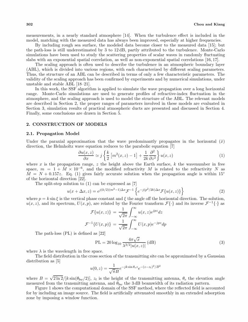
Figure 1 shows the computational domain of the SSF method, where the reflected field is accountedfor by including an image source. The field is artificially attenuated smoothly in an extended adsorptionzone by imposing a window function.

Progress In Electromagnetics Research B, Vol. 60, 2014 303

Figure 1. Computational domain including an image source and imposed with a window function.

2.2. Refractive-index Fluctuation

The total refractive index can be decomposed as

n(x, z) = n(z) + nf (x, z) (4)

where n(z) is the average refractive index and nf (x, z) the refractive-index fluctuation. A two-dimensional version of the latter can be realized with Monte-Carlo simulation as [16, 23]

n(s)f (x, z) =

∞∑p=1

∞∑q=1

a(s)pq sin (ζxpx + ζzqz) + b(s)

pq cos (ζxpx + ζzqz) (5)

where s is the realization index, ζxp the pth wavenumber, and apq and bpq are random numbers withvariance σ2

pq, which can be expressed as σ2pq = 4ΔζxpΔζzqFn(ζxp, ζzq), where Fn(ζx, ζz) is the two-

dimensional power spectral density of the refractive-index fluctuation.By applying the Wiener-Khinchin theorem [24], the two-dimensional power spectral density of an

isotropic Kolmogorov turbulence can be derived from its three-dimensional counterpart as [25]

FKn (ζx, ζz) =

0.0555C2n(

ζ2x + ζ2

z + 1/L20

)4/3(6)

where L0 is the outer scale, and C2n is the structure constant. A two-dimensional anisotropic Kolmogorov

spectrum can be modified from (6) as [25]

FKn (ζx, ζz) =

0.0555C2n(L0xL0z)4/3(

ζ2xL2

0x + ζ2z L2

0z + 1)4/3

(7)

where L0z and L0x are the outer scales in the vertical and the horizontal directions, respectively.The constraint of applying a 2D propagation scheme to predict 3D turbulence effects has been

discussed [26]. The phase variance of the 2D model is slightly overestimated. The log-amplitudevariances of 3D and 2D models agree well in the Fraunhofer region, but the 2D model tends tounderestimate the variance in the Fresnel region.

3. ESTIMATION OF PARAMETERS

The refractivity (N) of the atmosphere at microwave frequencies is related to the refractive index (n)as n = 1 + N × 10−6. It can be empirically estimated as N = (77.6/T )(P + 4810e/T ) [27, 28], where Tis the absolute temperature (in K), P = Pd + e is the atmospheric pressure (in hPa), Pd is the dry-air

304 Chou and Kiang

pressure, and e is the water vapor pressure (in hPa). The modified refractivity (M) is related to N asM = N + 106 × z/Re [2], where Re = 6.371× 106 (m) is the mean Earth radius, and z (m) is the heightabove the Earth surface.

The dry-air pressure can be derived from barometric formula, Pd = P0e−gmz/(RT0) [29], where

P0 = 1013.25 (in hPa) is the standard reference pressure, g = 9.8 (in m/s2) is the acceleration ofgravity, m = 0.0289644 (in kg/mol) is the molar mass of dry air, R = 8.31447 (in J/mol/K) is the idealgas constant, and T0 (in K) is the temperature at sea level.

The water vapor pressure (e) is related to the humidity mixing ratio (Q) (in g/kg) as e =QPd/622 [30]. The potential temperature (θ) is defined as θ = T (P0/P )R/cp [31], where R = 287.04 (inJ/K/kg) is the ideal gas constant of dry air, and cp = 1005 (in J/K/kg) is the specific heat capacity ofdry air under a constant pressure, R/cp � 0.286.

3.1. Scaling Approach on ABL’s

The scaling approach has been used to describe the turbulence in the atmospheric boundary layer(ABL) [18], with the ABL divided into several regions, each characterized by a set of scaling parameters.Fig. 2 shows the idealized scaling regions, in an unstable ABL (Lmo < 0) and a stable ABL (Lmo > 0),respectively [18]. The major scaling parameters in each region are listed in the parentheses, assumingthat the ABL is horizontally homogeneous, without clouds or fogs.

The Monin-Obukhov length (Lmo) is a scaling parameter for characterizing the surface layer;the local Monin-Obukhov length (Λ) is a local scaling parameter for characterizing the stratificationphenomenon above the surface layer in a stable ABL; u∗ is the velocity scale of the friction velocity,u∗0 is the friction velocity in the surface layer, which is nearly independent of height; and w∗ is theconvective velocity scale in an unstable ABL.

The shear-dominated surface layers, 0.01 < z/h < 0.1, −z/Lmo < 0.5, −h/Lmo < 5 ∼ 50 inFig. 2(a) and z/h < 0.1, h/Lmo < 10, z/Λ < h/Λ− 10 in Fig. 2(b), can be characterized by the Monin-Obukhov similarity theory, with the parameters u∗0, z and Lmo. The curve, z/Λ = h/Λ − 10, dividesthe z-less scaling layer and the intermittency layer. The local Monin-Obukhov length is related to Lmo

as Λ = Lmo(1 − z/h)α3 , where α3 is an empirical parameter.In Fig. 2(a), the ABL to the right of the dashed line, −z/Lmo � 0.5, is driven to a convective

state. When −z/Lmo > 1, the convective process dominates, leading to a free convection layer(0.01 < z/h < 0.1) or a mixed layer (0.1 < z/h < 0.8). The characteristics of a mixed layer becomesindependent of −h/Lmo once the ABL is driven into the convective state (−z/Lmo > 0.5). A near-neutral upper layer (0.1 < z/h < 0.8, −z/Lmo < 1) appears over land under low solar insolationor strong winds, and is frequently observed above the sea. In the entrainment layer (−h/Lmo > 1,

(a) (b)

Figure 2. Idealized scaling regions in (a) an unstable ABL and (b) a stable ABL [18, 32].

Progress In Electromagnetics Research B, Vol. 60, 2014 305

0.8 < z/h < 1.2), the turbulent structure is affected by the atmosphere above the ABL.A stable ABL can form over land during night-time when the surface is cooled via long-wavelength

emission. It can also form over sea via advection of warm air. Under stable conditions, the turbulenceof mechanical origin is suppressed by a negative heat flux on the surface. The thickness of boundarylayer (h) is typically an order of magnitude smaller than that under unstable conditions.

In a stable ABL, the stratification process leads to small eddies, with smaller outer scale comparedto that in a neutral or unstable ABL. Although the structure of a stable ABL is quite different from thatof an unstable ABL, the turbulence in the surface layer can still be described with the Monin-Obukhovsimilarity theory with parameters u∗0, z and Lmo.

The local Monin-Obukhov length can be applied when h/Lmo > 1 and z/h > 0.1, in which theturbulent variables are expressed in terms of z/Λ. As shown in Fig. 2(b), the boundary between thelocal scaling layer and the z-less scaling layer appears around z/Λ = 1. As z/Λ becomes larger, thedependence on z becomes weaker and finally disappears beyond z/Lmo = 1 (dashed line), in which casethe eddies are reduced in size and their vertical motion is inhibited by the stabilizing stratification. Theturbulent eddies stop being affected by the surface, and the dimensionless quantities, like Richardsonnumber, approach constant values. This phenomenon is called z-less stratification.

In the intermittency layer (z/Λ > h/Λ− 10) shown in Fig. 2(b), the turbulence becomes very weakand sporadic, no longer continuous in time and space. The intermittency layer is expected to touch thesurface at low wind speed or high stability.

Continuous turbulence may appear at relatively small h/Lmo. The z-less region may expand withh/Lmo, up to h/Lmo � 5, then is restrained by the intermittency layer from above.

3.2. Monin-Obukhov Length

The Monin-Obukhov length is defined as [33]

Lmo =T0

gka

u2∗0

θ∗0(8)

where g = 9.8 (m/s2) is the acceleration of gravity, ka = 0.4 is the von Karman constant, T0 (K) is thereference temperature; u∗0 and θ∗0 are the friction velocity and the temperature scales, respectively,near the surface.

The Monin-Obukhov length is essentially determined by the heat flux and the friction velocity,which are nearly independent of height within the surface layer. The atmosphere can be generallycharacterized in terms of z/Lmo as follows [34]: When z/Lmo is a large negative number, the heatconvection dominates. When z/Lmo is a small negative number, the mechanical turbulence dominates.When z/Lmo = 0, only mechanical turbulence contributes. When z/Lmo is a small positive number,the mechanical turbulence is slightly damped by the temperature stratification. When z/Lmo is a largepositive number, the mechanical turbulence is severely reduced by the temperature stratification. Insummary, z/Lmo quantifies the relative significance between heat convection and mechanical turbulenceduring the day-time, and to what extent the stratification suppresses the mechanical turbulence duringthe night-time.

3.3. Height of Boundary Layer

The height of the boundary layer (h) also known as the mixing height, is not uniquely defined. In [35],it is defined as the height of the layer adjacent to the ground over which pollutants or similar substancesemitted within this layer or entrained into it become vertically dispersed by convection or mechanicalturbulence, within a time scale of about an hour.

In the entrainment layer of a typical convective boundary layer (CBL), the constituents are notwell mixed and the turbulence intensity declines towards its top surface [36, 37]. The thickness of theentrainment layer is typically 30% of the mixed layer. Another definition of the convective mixing heightis the height where the heat flux gradient reverses its sign.

A stable boundary layer (SBL) can be divided into two sublayers, a layer of continuous turbulenceand an outer layer of sporadic or intermittent turbulence. Under very stable conditions, the layer ofsporadic turbulence may extend to the ground, as shown in Fig. 2(b) [18]. The scaling height of an SBL

306 Chou and Kiang

generally refers to the layer of continuous turbulence since it is very difficult to measure sporadic orintermittent turbulence. Similar to the CBL, the turbulence is not strictly confined to the region belowh.

A neutral boundary layer is formed when the heat flux approaches zero, under either stable orunstable condition. The wind shear is the main source of turbulence, and the neutral boundary layermay extend above the ABL.

The boundary layer height can be estimated using empirical formulas derived from measurementor numerical data. Based on the scaling approach, the layer height under stable conditions can beexpressed as h = a1LE = a1u∗0/fc [35] or h = a2

√LELmo = a2

√u∗0Lmo/fc, where LE = u∗0/fc is the

Ekman length; a1 = 0.07–0.3 and a2 = 0.3–0.7 are empirical coefficients; fc = 2Ω sin ϕ is the Coriolisparameter at latitude ϕ, with Ω = 7.27 × 10−5 rad/s, the angular speed of the Earth’s rotation. Notethat a neutral, stationary boundary layer is assumed, and 1/fc is generally much longer than relevanttime scales. In this work, the mixing height of a CBL is estimated as the height where the first potentialtemperature inversion takes place.

3.4. Structure Constant

The structure constant (C2n) usually becomes large near the Earth’s surface and in the clouds [38]. The

magnitude of C2n generally increases with longer wavelength. It falls, near the ground, in the range of

10−16 to 10−12 m−2/3 in the visible and the infrared bands [39]; and is orders of magnitude larger inthe near-millimeter-wave band than in the infrared.

The structure constant can be estimated using the Kolmogorov-Corrsin formula, C2n =

βnNnε−1/3 [40], where βn = 2.8 is the Kolmogorov constant [25], and ε is the dissipation rate of theturbulent kinetic energy (TKE). The outer scale of the turbulence in direction i (L0i) can be estimatedfrom the eddy diffusivity (Ki) and the TKE dissipation rate (ε) as L0i = (Ki/ε

1/3)3/4 [25]. Thus, thestructure constant can be expressed as [25, 41]

C2n � βn

(∂〈n〉∂z

)2

L4/30z (9)

In a marine planetary boundary layer (MPBL), the near-surface turbulence leads to relatively largemoisture fluctuation [42], which plays a dominant role, as compared to temperature, in determining C2

nin microwave bands and significantly affects C2

n in acoustic and optical bands. The over-land simulationshows a larger diurnal variation, but the moisture fluctuation does not play a dominant role. Nearthe surface, the temperature makes a comparable contribution to C2

n in microwave bands, particularlyin the afternoon. In the acoustic and optical bands, C2

n is primarily determined by the temperaturefluctuations.

3.5. Outer Scales of Random Medium

A model of eddy diffusivity, based on the diffusion theory and the Eulerian statistical method [11], canbe used in the ABL under all stability conditions, except the very stable cases in which the Monin-Obukhov scaling theory does not apply. The eddy diffusivity in a shear-buoyancy ABL can be expressedas [11]

Ki = σib ib + σis is (10)

where σ2ib and σ2

is are the Lagrangian variances of the ith component of the turbulent wind field, dueto buoyancy and wind shear, respectively; ib and is are the Lagrangian lengths due to buoyancy andwind shear, respectively. The interaction between shear and buoyancy is neglected.

The convective velocity scale, under unstable conditions (Lmo < 0), can be expressed as [11]

w∗ = u∗0(− h

kaLmo

)1/3

(11)

The friction velocity can be expressed as [43]

u∗ = u∗0(1 − z/h)α (12)

Progress In Electromagnetics Research B, Vol. 60, 2014 307

where α depends on the state of the boundary layer, and α = 1 [43] is used in this work.Under an unstable condition, the surface potential temperature is higher than the air potential

temperature, u∗ (characterizing the wind-shear effect) and w∗ (characterizing air convection) willdominate the air turbulence. Under a stable condition, the surface potential temperature is lower thanthe air potential temperature, the air turbulence is dominated by u∗, and the stabilizing stratificationcan be characterized by z/Λ.

The eddy diffusivity in the boundary layer (z/h ≤ 1), under unstable conditions (Lmo < 0), can beexpressed as

K(u)i = K

(u)ci + K

(u)mi (13)

where K(u)ci = C1iw∗z and K

(u)mi = C2iu∗z are the convective and the wind-shear turbulence components,

respectively, with

C1z =0.16 (−0.01h/Lmo)

1/2

(z/h)(1 − e−4z/h − 0.0003e8z/h

)−4/3

C2z = 0.4/ (1 + 15fcz/u∗0)4/3

C1x = 0.1086 (−0.01h/Lmo)1/2 /(z/h)

C2x = 4.913/ (1 + 116.7fcz/u∗0)4/3

(14)

Figure 3(a) shows the distribution of K(u)cz /K

(u)mz (in log scale) on the −h/Lmo-z/h plane, where the

Coriolis term in (14) is ignored. The value of K(u)cz /K

(u)mz is roughly a constant in each region labeled in

Fig. 2(a).

(a) (b)

Figure 3. Distribution of (a) log10[K(u)cz /K

(u)mz ] and (b) log10[K

(u)cx /K

(u)mx] on the −h/Lmo-z/h plane, in

an unstable ABL.

Figure 3(b) shows the distribution of K(u)cx /K

(u)mx (in log scale) on the −h/Lmo-z/h plane. The

convective turbulence still dominates as the instability gets stronger, but its influence decreases athigher altitudes in the ABL.

Under stable conditions (Lmo > 0), on the other hand, we have

K(s)z =

0.4(1 + 3.7z/Λ)1/3

(1 + 15fcz/u∗0 + 3.7z/Λ)4/3u∗z

K(s)x =

4.9(1 + 3.7z/Λ)1/3

(1 + 116.7fcz/u∗0 + 3.7z/Λ)4/3u∗z

(15)

Figure 4 shows the distributions of K(s)z /(u∗0z) and K

(s)x /(u∗0z) on the h/Lmo-z/h plane, in which

the Coriolis term in (15) is ignored. Both ratios are roughly constant in each region labeled in Fig. 2(b).

308 Chou and Kiang

(a) (b)

Figure 4. Distribution of (a) K(s)z /(u∗0z) and (b) K

(s)x /(u∗0z) on the h/Lmo-z/h plane in a stable

ABL.

The outer scales under unstable conditions (Lmo < 0) can be expressed as

L(u)0z =z

1

[3.125(1−z/h)3−1.625z/Lmo]1/4

{0.0217 (−h/Lmo)

5/6 (z/h)−1(1−e−4z/h−0.0003e8z/h

)−4/3+

0.4(1−z/h)

(1+15fcz/u∗0)4/3

}3/4

L(u)0x =z

1

[3.125(1 − z/h)3 − 1.625z/Lmo]1/4

{0.01474 (−h/Lmo)

5/6

(z/h)+

4.913(1 − z/h)

(1 + 116.7fcz/u∗0)4/3

}3/4(16)

When the convective mechanism dominates the turbulence, as in the free convection layer and the mixedlayer labeled in Fig. 2(a), they reduce to

L(u)0cz =

0.05 (−h/Lmo)3/8

(z/h)z

(1 − e−4z/h − 0.0003e8z/h

)

L(u)0cx =

0.0375 (−h/Lmo)3/8

z/hz

(17)

The outer scales, under stable conditions (Lmo > 0), can be expressed as

L(s)0z =

0.3783z(1 + 15fcz/u∗0 + 3.7z/Λ)

L(s)0x =

2.477z(1 + 116.7fcz/u∗0 + 3.7z/Λ)

(18)

Under strongly stable condition, they reduce to

L(s)0z � 0.102Lmo

L(s)0x � 0.669Lmo

(19)

with the anisotropy L(s)0x /L

(s)0z � 6.56, which is independent of z and consistent with the z-less layer

(Λ � Lmo) labeled in Fig. 2(b). Since the turbulence above the ABL is very weak, the outer scales areapproximated as zero in this work.

4. SIMULATIONS AND DISCUSSIONS

Simulations will be conducted to compare with the observation data over the Gulf area (50◦N, 28◦E) onApril 28, 1996, which is a typical shamal day, according to the US Navy Ship Antisubmarine WarfareReadiness/ Effectiveness Measuring programme (SHAREM-115) [44, 45].

Progress In Electromagnetics Research B, Vol. 60, 2014 309

This case is presented because the data are well validated and involve the whole Gulf orography.Here, shamal means the strong north-westerly winds in this area, which blow frequently in both warmand cold seasons [46]. Shamals are important weather phenomena in the Gulf region as they causeadverse weather conditions, including gusty winds, sand-storms, dust-storms, rough seas, low-level windshear, and so on. Summer shamals affect the Gulf region predominantly during May to July, and areknown to be linked with the seasonal thermal flows over north-west India, Pakistan, Iran and southernSaudi Arabia.

The boundary layer structure over the Gulf is strongly influenced by the surrounding desertlandmass. Warm dry air flows from the desert over the relatively cool waters of the Gulf, leadingto a stable internal boundary layer. The layer evolves and eventually forms a new marine ABL. Thestable stratification tends to suppress vertical mixing and trap moisture within the layer, leading to anincrease in refractive index and the formation of a strong atmospheric duct [44].

Ducts form over land and sea at nights. Over the land, ducts are formed by the temperatureinversion attributed to radiative cooling near the surface. During the daytime, ducts disappear fromthe land except the south-east area of the southern Gulf coast, where the air in the convective boundarylayer over land is well mixed vertically to create strong gradient of refractive index.

In the air over the waters of the Gulf, the humidity at low-level is high, which sustains the ducts inboth time and space. This marine boundary layer (MBL), accompanied by the ambient wind and theland-sea temperature difference of up to 10◦C, has the characteristics of a marine internal boundarylayer (MIBL) [47]. An MIBL is formed as the air mass moves from a hot dry surface to a cool watersurface [44]. The MIBL’s are modified by meso-scale structures and diurnal variations [48, 49]. Withinabout 100 km of the shore, simple surface ducts take shape as a consequence of the increased humidity

(a) (b)

(c)

Figure 5. (a) Wind speeds, (b) potential temperature and (c) temperature on April 28, 1996, ——:(27◦46’N, 50◦45’E) at 1400 UTC (stable ABL), from the control run [45]; —◦—: (26◦09’N, 53◦06’E)at 1330 UTC (stable ABL), from the rawinsonde observation [44]; ——: (29◦13’N, 47◦59’E) (KuwaitInternational Airport) at 1200 UTC (unstable ABL), from the coastal synoptic reporting stations [44].

310 Chou and Kiang

in the near-surface layer below the temperature inversion height. Beyond 100 km of the shore, furtherincrease of near-surface moisture may transform a surface duct to a surface-based duct. Farther inthe downwind direction, the increased cooling at the top of the trapping layer creates a minimum ofmodified refractivity, with its value larger than that at the surface, and an elevated duct is formed.

Figures 5(a), 5(b) and 6(a) show the measurement data of wind speed (m/s), potential temperature(K) and humidity mixing ratio (g/kg), respectively. Some curves are produced by using the mesoscalemodel (MM5V3), at the grid size of 25 km, based on the observed data at different locations [45]. Somecurves are compiled from the rawinsonde observation and the coastal synoptic reporting stations [44],respectively.

Figure 5(c) shows the temperature profiles derived from the potential temperature in Fig. 5(b)and humidity mixing ratio in Fig. 6(a). Fig. 6(b) shows the profiles of modified refractivity, using thetemperature in Fig. 5(c) and the humidity mixing ratio in Fig. 6(a). The curve produced with MM5V3indicates a ducting layer over the height of 200–350 m. The curve with rawinsonde observation indicatestwo ducting layers, one below 80 m and the other over 250–300 m.

(a) (b)

Figure 6. (a) Humidity mixing ratio and (b) modified refractivity, with the same parameters as inFig. 5.

Table 1 lists the Monin-Obukhov length (Lmo), the surface friction velocity (u∗0), and the surfacetemperature scale (θ∗0), which are derived from the profiles of wind speed in Fig. 5(a) and potentialtemperature in Fig. 5(b) [44, 45]. The mixing height (h) is derived using the approach described inSection 3.3.

Table 1. Parameters derived from measurements on April 28, 1996 [44, 45].

case Lmo (m) u∗0 (m/s) θ∗0 (K) h (m) latitude (N) longitude (E) Time (UTC)

1 407 0.1509 0.0042 288 27◦46’ 50◦45’ 1400

2 311 0.8204 0.1643 717 26◦09’ 53◦06’ 1330

3 −167 1.3131 −0.8140 1732 29◦13’ 47◦59’ 1200

Figures 7(a), 7(b) and 8(a) show the vertical and horizontal outer scales, as well as the anisotropyof outer scales, based on the parameters, Lmo, h and u∗0, listed in Table 1.

The parameters in case 1 of Table 1 are associated with the curves produced with MM5V3. Asshown in Fig. 2(b), a near neutral upper layer may appear above the surface layer. Under a nearneutral condition (small z/Λ), the horizontal outer scales are significantly reduced, leading to a smalleranisotropy (L0x/L0z). The anisotropy decreases to a minimum in the surface layer, in which the Coriolisterm (fcz/u∗0) dominates; then increases as the stratification term becomes more important; and mayreach a constant at large z/Λ.

Progress In Electromagnetics Research B, Vol. 60, 2014 311

(a) (b)

Figure 7. (a) Vertical outer scale and (b) horizontal outer scale, parameters are the same as in Fig. 5.

(a) (b)

Figure 8. (a) Anisotropy of outer scales and (b) structure constant, parameters are the same as inFig. 5.

The parameters in case 2 of Table 1 are associated with the rawinsonde curves, representing amore stable condition (large z/Λ). The outer scales (L0x and L0z) are much smaller than those underunstable conditions [50], as shown in Fig. 7. The outer scales under stable conditions are determined byboth the Coriolis term (fc/u∗0) and the stratification term (z/Λ). Under a more stable condition, theanisotropy becomes larger due to the vertical compression of air turbulence by a cold surface. It canalso be explained using (18), in which the Coriolis term (fcz/u∗0) has stronger effect on the horizontalouter scale than on the vertical one. The characteristics of case 2, as shown in Figs. 7 and 8(a), appearmore like a z-less layer than a local scaling layer.

In an unstable ABL, the eddies tend to be vertically elongated by convection, leading to a smallerL0x/L0z. The characteristics of case 3 (coastal synoptic curves), with −h/Lmo = −10.4, appear morelike a convective boundary layer as labeled in Fig. 2(a). Note that the horizontal outer scale canbe increased by wind shear (u∗0), and the vertical outer scale can be increased by high temperaturevariation (θ∗0).

Figure 8(b) shows the structure constant estimated using (9), based on the data of average modifiedrefractivity in Fig. 6(b) and vertical outer scale in Fig. 7(a). In case 3, the structure constant is arelatively smooth function of height, because the vertical outer scale is large and the average modifiedrefractivity is a smooth function of height. However, the structure constant around the ducting regionis much smaller than that under stable conditions like cases 1 and 2. Around the ducting region of cases1 and 2, L0z is relatively small, and the variation of average modified refractivity is relatively large,leading to large C2

n.Figures 9 and 10 show the distributions of path-loss in a stable ABL, indicating a surface-based duct

and a complex duct, respectively. In Fig. 9, the ducting effect is observed below 300 m. A shadowing

312 Chou and Kiang

region appears at low altitude around the range of 50 km, indicating a less steady communication channeltherein, as compared to an evaporation duct or a surface duct. This feature is attributed to the baselayer of the surface-based duct, as shown in the MM5V3 curve of Fig. 6(b). The turbulence reduces the

(a) (b)

Figure 9. Distribution of path-loss in a stable ABL, with the parameters from —– curves in Figs. 6(b),7, and 8(b), zt = 4 m, f = 10.6 GHz; (a) without turbulence, (b) with turbulence.

(a) (b)

Figure 10. Distribution of path-loss in a stable ABL, with the parameters from —◦— curves inFigs. 6(b), 7, and 8(b), zt = 4m, f = 10.6 GHz; (a) without turbulence, (b) with turbulence.

(a) (b)

Figure 11. Average path-loss within duct, −−−: without turbulence, ——: with turbulence; (a) datafrom Fig. 9, with z < 300 m; (b) data from Fig. 10, with z < 250 m.

Progress In Electromagnetics Research B, Vol. 60, 2014 313

(a) (b)

Figure 12. Distribution of path-loss in an unstable ABL, with the parameters from —— curves inFigs. 6(b), 7, and 8(b), zt = 4m, f = 10.6 GHz; (a) without turbulence, (b) with turbulence.

path-loss in that shadowing region by about 10 dB.In Fig. 10, a steady communication channel appears below 80 m due to the surface ducting layer

of the complex duct, as shown in the rawinsonde curve of Fig. 6(b). The ducting effect is less obviousabove 80 m, and a feeble duct appears below the height of 250 m. A shadowing region appears aroundthe range of 30 to 80 km and the height of 100 m. The path-loss therein is reduced by about 5 dB in thepresence of turbulence, although not so obvious as in Fig. 9.

In both Figs. 9 and 10, the turbulence seems to smear the border of duct, and the path-lossabove the duct is generally reduced. In summary, significant turbulence effects are observed within theducting region above the sea in daytime, under stable conditions, which can be attributed to the largerefractive-index gradient. The energy leakage from the ducting to the non-ducting regions, caused bythe turbulence, leads to a more uniform distribution of path-loss distribution within the duct.

Figure 11 shows the average path-loss within the duct, using the data in Figs. 9 and 10, respectively.It is observed that the turbulence effect reduces the variation of average path-loss over range.

Figure 12 shows distribution of path-loss in an unstable ABL without duct. The turbulence makesonly little difference.

5. CONCLUSION

A complete model has been proposed to study wave propagation in an atmospheric boundary layer(ABL), in the presence of air turbulence. All the relevant parameters are estimated on the atmosphericconditions, with the scaling parameters derived from the measurement data. A systematic approach,based on split-step Fourier propagation algorithm, has also been developed to simulate wave propagationin atmospheric ducts, with proper range of parameters closely related to the weather condition of theABL. A set of measurement data in the Gulf area is used to confirm the effectiveness of this approach.

ACKNOWLEDGMENT

This work was sponsored by the National Science Council, Taiwan, under contract NSC 100-2221-E-002-232; and the Ministry of Education, Taiwan, under Aim for Top University Project 103R3401-1.

REFERENCES

1. Mentes, S. S. and Z. Kaymaz, “Investigation of surface duct conditions over Istanbul, Turkey,” J.Appl. Meteorol. Climatol., Vol. 46, No. 3, 318–337, 2007.

2. Skolnik, M. I., Introduction to Radar Systems, 3rd edition, McGraw-Hill, 2001.

314 Chou and Kiang

3. Ulaby, F. T., R. K. Moore, and A. K. Fung, “Microwave remote sensing fundamentals andradiometry,” Microwave Remote Sensing: Active and Passive, Vol. 1, Addison-Wesley, 1981.

4. Kerans, A., A. S. Kulessa, E. Lensson, G. French, and G. S. Woods, “Implications of the evaporationduct for microwave radio path design over tropical oceans in Northern Australia,” Workshop Appl.Radio Sci., Leura, Australia, 2002.

5. Sirkova, I. and M. Mikhalev, “Parabolic-equation-based study of ducting effects on microwavepropagation,” Microwave Opt. Technol. Lett., Vol. 42, No. 5, 390–394, 2004.

6. Sirkova, I. and M. Mikhalev, “Influence of tropospheric duct parameters changes on microwave pathloss,” Proc. Int. Sci. Conf. Info. Commun. Energy Syst. Technol., 43–46, Sofia, Bulgaria, 2003.

7. Kuttler, J. R. and G. D. Dockery, “Theoretical description of the parabolic approximation/Fouriersplit-step method of representing electromagnetic propagation in the troposphere,” Radio Sci.,Vol. 26, No. 2, 381–393, 1991.

8. Douchin, N., S. Bolioli, F. Christophe, and P. Combes, “Theoretical study of the evaporation ducteffects on satellite-to-ship radio links near the horizon,” IEE Proc. Microwaves Antennas Propagat.,Vol. 141, No. 4, 272–278, 1994.

9. Apaydin, G. and L. Sevgi, “FEM-based surface wave multimixed-path propagator and path losspredictions,” IEEE Antennas Wireless Propagat. Lett., Vol. 8, 1010–1013, 2009.

10. Essen, H. and H. H. Fuchs, “Microwave and millimeterwave propagation within the marineboundary layer,” German Microwave Conf., Karlsruhe, Germany, 2006.

11. Degrazia, G. A., D. Anfossi, J. C. Carvalho, C. Mangia, T. Tirabassi, and H. F. C. Velho,“Turbulence parameterisation for PBL dispersion models in all stability conditions,” Atmos.Environ., Vol. 34, No. 21, 3575–3583, 2000.

12. Kukushkin, A. and J. Wiley, Radio Wave Propagation in the Marine Boundary Layer, Wiley OnlineLibrary, 2004.

13. Rouseff, D., “Simulated microwave propagation through tropospheric turbulence,” IEEE Trans.Antennas Propagat., Vol. 40, No. 9, 1076–1083, 1992.

14. Hitney, H. V., “A practical tropospheric scatter model using the parabolic equation,” IEEE Trans.Antennas Propagat., Vol. 41, No. 7, 905–909, 1993.

15. Hitney, H. V., “Evaporation duct propagation and near-grazing angle scattering from a rough sea,”IEEE Int. Geosci. Remote Sensing Symp., 2631–2633, 1999.

16. Bein, G., “Monte Carlo computer technique for one-dimensional random media,” IEEE Trans.Antennas Propagat., Vol. 21, No. 1, 83–88, 1973.

17. Adams, R. N. and E. D. Denman, Wave Propagation and Turbulent Media, Elsevier, 1966.18. Holtslag, A. A. M. and F. T. M. Nieuwstadt, “Scaling the atmospheric boundary layer,” Boundary

Layer Meteorol., Vol. 36, No. 1, 201–209, 1986.19. Kaimal, J. C., J. C. Wyngaard, D. A. Haugen, O. R. Cote, Y. Izumi, S. J. Caughey, and

C. J. Readings, “Turbulence structure in the convective boundary layer,” J. Atmos. Sci., Vol. 33,No. 11, 2152–2169, 1976.

20. Moeng, C.-H., “A large-eddy-simulation model for the study of planetary boundary-layerturbulence,” J. Atmos. Sci., Vol. 41, No. 13, 2052–2062, 1984.

21. Nieuwstadt, F. T. M., “The turbulent structure of the stable, nocturnal boundary layer,” J. Atmos.Sci., Vol. 41, No. 14, 2202–2216, 1984.

22. Levy, M., Parabolic Equation Methods for Electromagnetic Wave Propagation, Inst. Electr. Eng.,2000.

23. Frehlich, R., “Simulation of laser propagation in a turbulent atmosphere,” Appl. Opt., Vol. 39,No. 3, 393–397, Jan. 2000.

24. Wiener, N., “Generalized harmonic analysis,” Acta Mathematica, Vol. 55, No. 1, 117–258, 1930.25. Ishimaru, A., Wave Propagation and Scattering in Random Media, IEEE Press, 1997.26. Fabbro, V. and L. Feral, “Comparison of 2D and 3D electromagnetic approaches to predict

tropospheric turbulence effects in clear sky conditions,” IEEE Trans. Antennas Propagat., Vol. 60,No. 9, 4398–4407, 2012.

Progress In Electromagnetics Research B, Vol. 60, 2014 315

27. Smith, E. K. and S. Weintraub, “The constants in the equation for atmospheric refractive index atradio frequencies,” Proc. IRE, Vol. 41, 1035–1037, 1953.

28. Bean, B. R. and E. Dutton, Radio Meteorology, Dover Publications, 1968.29. Berberan-Santos, M. N., E. N. Bodunov, and L. Pogliani, “On the barometric formula,” Am. J.

Phys., Vol. 65, 404, 1997.30. Wallace, J. M. and P. V. Hobbs, Atmospheric Science: An Introductory Survey, Academic Press,

2006.31. Arya, P. S., Introduction to Micrometeorology, 2nd edition, Academic press, 2001.32. Yamartino, R. J., J. S. Scire, G. R. Carmichael, and Y. S. Chang, “The CALGRID mesoscale

photochemical grid model. I. Model formulation,” Atmos. Environ. Part A, Vol. 26, No. 8, 1493–1512, 1992.

33. De Bruin, H. A. R., R. J. Ronda, and B. J. H. Van De Wiel, “Approximate solutions for theObukhov length and the surface fluxes in terms of bulk Richardson numbers,” Boundary LayerMeteorol., Vol. 95, No. 1, 145–157, 2000.

34. Panovsky, H. A. and J. A. Dutton, Atmospheric Turbulence: Models and Methods for EngineeringApplications, John Wiley, 1984.

35. Seibert, P., F. Beyrich, S.-E. Gryning, S. Joffre, A. Rasmussen, and P. Tercier, “Review andintercomparison of operational methods for the determination of the mixing height,” Atmos.Environ., Vol. 34, No. 7, 1001–1027, 2000.

36. Gryning, S.-E. and E. Batchvarova, “Parameterization of the depth of the entrainment zone abovethe daytime mixed layer,” Quart. J. Royal Meteorol. Soc., Vol. 120, No. 515, 47–58, 1994.

37. Sun, J., W. Jiang, Z. Chen, and R. Yuan, “Parameterization for the depth of the entrainment zoneabove the convectively mixed layer,” Adv. Atmos. Sci., Vol. 22, No. 1, 114–121, 2005.

38. Cox, D. C., H. W. Arnold, and H. H. Hoffman, “Observations of cloud-produced amplitudescintillation on 19- and 28-GHz Earth-space paths,” Radio Sci., Vol. 16, No. 5, 885–907, 1981.

39. Tunick, A., “Optical turbulence effects on ground to satellite microwave refractivity,” DTICDocument ADA449682, 2006.

40. Andreas, E. L., “On the Kolmogorov constants for the temperature-humidity cospectrum and therefractive index spectrum,” J. Atmos. Sci., Vol. 44, No. 17, 2399–2406, 1987.

41. Tatarskii, V. I., The Effects of the Turbulent Atmosphere on Wave Propagation, Israel Program forScientific Translations, 1971.

42. Burk, S. D., “Refractive index structure parameters-time-dependent calculations using a numericalboundary-layer model,” J. Appl. Meteorol., Vol. 19, 562–576, 1980.

43. Gryning, S. E., E. Batchvarova, B. Brummer, H. Jørgensen, and S. Larsen, “On the extension ofthe wind profile over homogeneous terrain beyond the surface boundary layer,” Boundary LayerMeteorol., Vol. 124, No. 2, 251–268, 2007.

44. Brooks, I. M., A. K. Goroch, and D. P. Rogers, “Observations of strong surface radar ducts overthe Persian Gulf,” J. Appl. Meteorol., Vol. 38, No. 9, 1293–1310, 1999.

45. Atkinson, B. W. and M. Zhu, “Radar-duct and boundary-layer characteristics over the area of theGulf,” Q. J. R. Meteorol. Soc., Vol. 131, No. 609, 1923–1953, 2005.

46. Rao, P. G., H. R. Hatwar, M. H. Al-Sulaiti, and A. H. Al-Mulla, “Summer shamals over the ArabianGulf,” Weather, Vol. 58, No. 12, 471–478, 2003.

47. Garratt, J. R. and B. F. Ryan, “The structure of the stably stratified internal boundary layer inoffshore flow over the sea,” Boundary-Layer Meteorol., Vol. 47, No. 1, 17–40, 1989.

48. Plant, R. S. and B. W. Atkinson, “Sea-breeze modification of the growth of a marine internalboundary layer,” Boundary Layer Meteorol., Vol. 104, No. 2, 201–228, 2002.

49. Zhu, M. and B. W. Atkinson, “Observed and modelled climatology of the land-sea breeze circulationover the Persian Gulf,” Int. J. Climatol., Vol. 24, No. 7, 883–905, 2004.

50. Ludi, A. and A. Magun, “Near-horizontal line-of-sight millimeter-wave propagation measurementsfor the determination of outer length scales and anisotropy of turbulent refractive index fluctuationsin the lower troposphere,” Radio Sci., Vol. 37, No. 2, 12-1–19, 2002.