Chapter 4 Duality in Linear Programming

Companion slides of Applied Mathematical Programming

by Bradley, Hax, and Magnanti (Addison-Wesley, 1977)

prepared by José Fernando Oliveira

Maria Antónia Carravilla

What is duality?

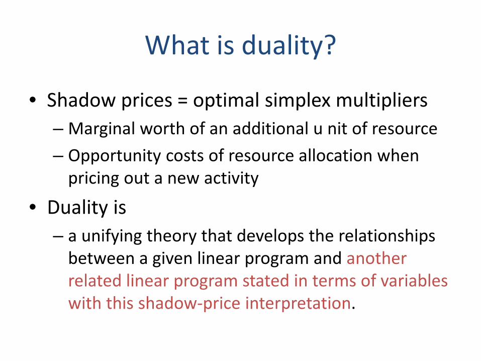
• Shadow prices = optimal simplex multipliers – Marginal worth of an additional u nit of resource – Opportunity costs of resource allocation when

pricing out a new activity

• Duality is – a unifying theory that develops the relationships

between a given linear program and another related linear program stated in terms of variables with this shadow-price interpretation.

This unified theory is important

1. Because it allows fully understanding the shadow-price interpretation of the optimal simplex multipliers, which can prove very useful in understanding the implications of a particular linear-programming model.

2. Because it is often possible to solve the related linear program with the shadow prices as the variables in place of, or in conjunction with, the original linear program, thereby taking advantage of some computational efficiencies.

A PREVIEW OF DUALITY

A preview of duality

Firm producing three types of automobile trailers:

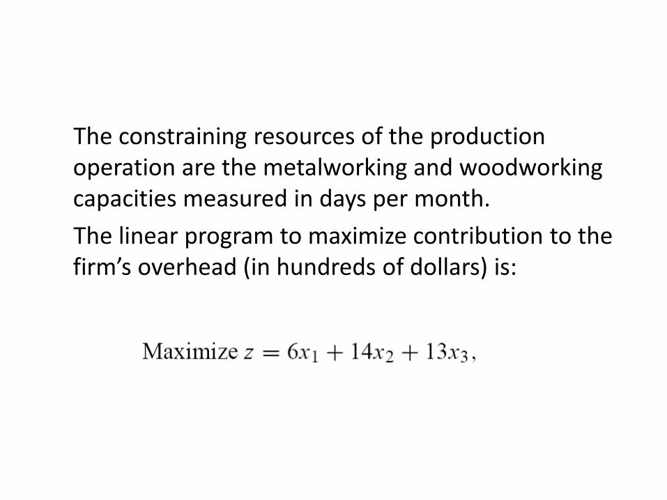
The constraining resources of the production operation are the metalworking and woodworking capacities measured in days per month. The linear program to maximize contribution to the firm’s overhead (in hundreds of dollars) is:

subject to:

Initial tableau in canonical form

Final (optimal) tableau

• The shadow prices, y1 for metalworking capacity and y2 for woodworking capacity, can be determined from the final tableau as the negative of the reduced costs associated with the slack variables x4 and x5.

• Thus these shadow prices are y1 = 11 and y2 = 1/2, respectively.

Economic properties of the shadow prices associated with the resources

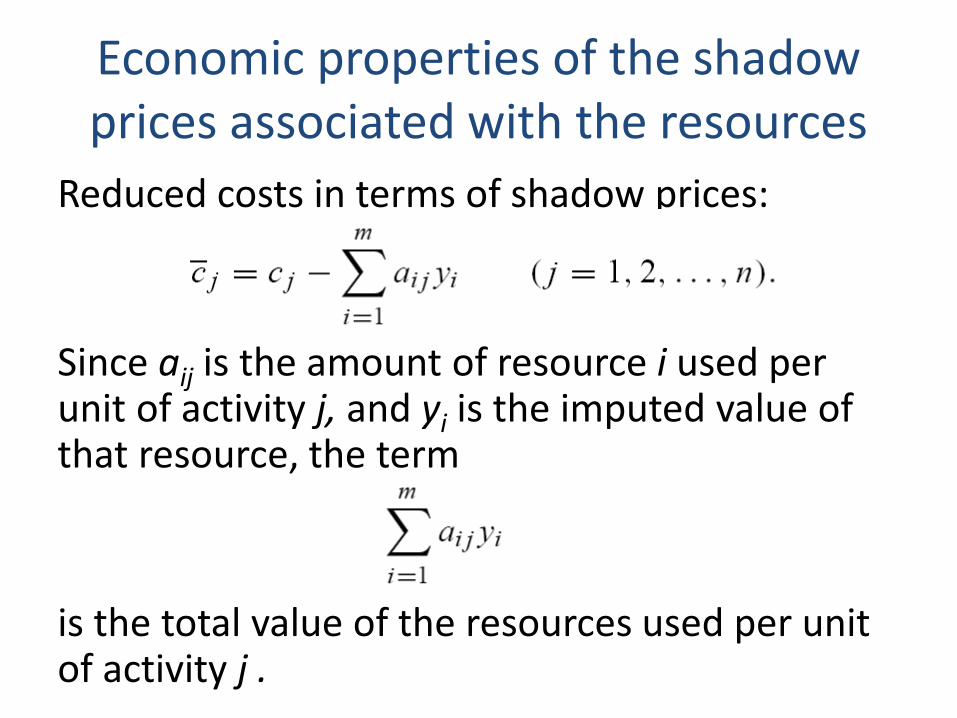
Reduced costs in terms of shadow prices:

Since aij is the amount of resource i used per unit of activity j, and yi is the imputed value of that resource, the term is the total value of the resources used per unit of activity j .

is thus the marginal resource cost for using activity j. If we think of the objective coefficients cj as being marginal revenues, the reduced costs are simply net marginal revenues (i.e., marginal revenue minus marginal cost).

• For the basic variables the reduced costs are zero. The values imputed to the resources are such that the net marginal revenue is zero on those activities operated at a positive level. That is, for any production activity at positive level, marginal revenue must equal marginal cost.

• The reduced costs for all nonbasic variables are negative. The interpretation is that, for the values imputed to the scarce resources, marginal revenue is less than marginal cost for these activities, so they should not be pursued.

Shadow prices are interpreted as the opportunity costs associated with

consuming the firm’s resources

If we value the firm’s total resources at the shadow prices, we find their value

is exactly equal to the optimal value of the objective function of the firm’s decision problem.

Can shadow prices be determined directly, without solving the firm’s production-

decision problem? • The shadow prices must satisfy the requirement that

marginal revenue be less than or equal to marginal cost for all activities.

• Further, they must be nonnegative since they are associated with less-than-or-equal-to constraints in a maximization decision problem.

Imagine that the firm does not own its productive capacity but has to rent it…

Shadow prices = rent rates

optimal solution is y1 = 11, y2 = 1/2 , and v = 294.

By solving (2), we can determine the shadow prices of (1) directly

PRIMAL DUAL

(1) (2)

Solving the dual by the simplex method solves the primal as well

• The decision variables do the dual give the shadow prices of the primal. y1 = 11, y2 = 1/2, and v = 294

• The shadow prices of the dual give the

decision variables of the primal. u1 = 36, u2 = 0, and u3 = 6

Implications of solving these problems by the simplex method

• The optimality conditions of the simplex method require that the reduced costs of basic variables be zero, i.e.:

(if a decision variable of the primal is positive, then the corresponding constraint in the dual must hold with equality)

Implications of solving these problems by the simplex method

• The optimality conditions require that the nonbasic variables be zero (at least for those variables with negative reduced costs), i.e.:

(if a constraint holds as a strict inequality, then the

corresponding decision variable must be zero)

Implications of solving these problems by the simplex method (chapter 3)

• If some shadow price is positive, then the corresponding constraint must hold with equality, i.e.:

• If a constraint of the primal is not binding, then its corresponding shadow price must be zero

Complementary slackness conditions

• If a variable is positive, its corresponding (complementary) dual constraint holds with equality.

• If a dual constraint holds with strict inequality, then the corresponding (complementary) primal variable must be zero.

DEFINITION OF THE DUAL PROBLEM FINDING THE DUAL IN GENERAL

Primal-Dual formalization

Generalization

Generalization

Generalization

THE FUNDAMENTAL DUALITY PROPERTIES

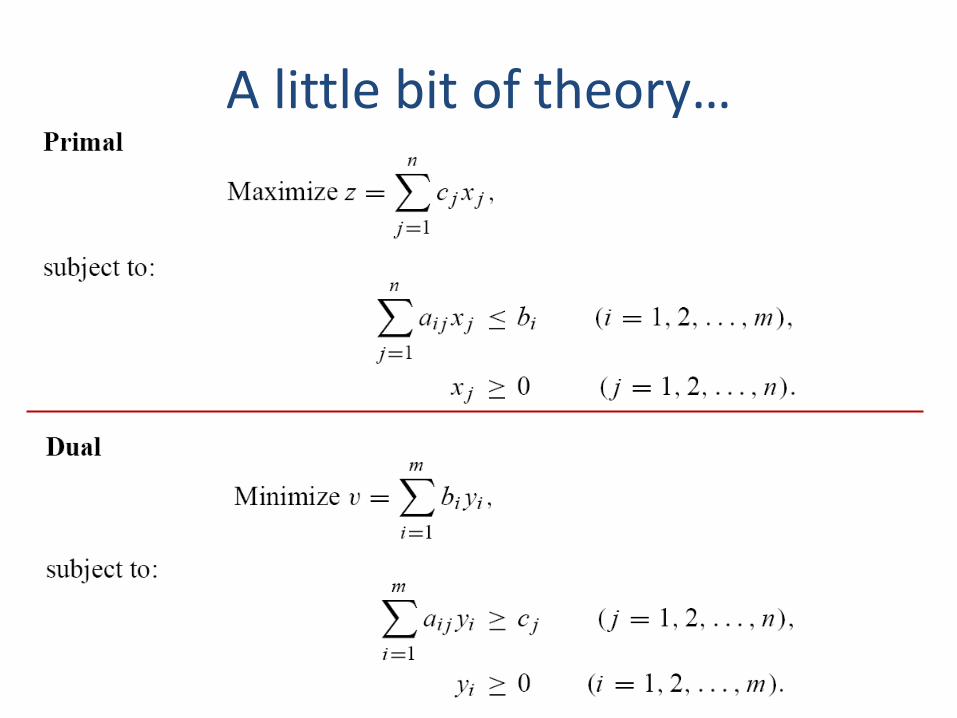
A little bit of theory…

Weak Duality Property

If is a feasible solution to the primal problem and is a feasible solution to the dual problem, then

Optimality Property

If is a feasible solution to the primal problem and is a feasible solution to the dual problem, then and they are both optimal for their problems.

Unboundedness Property

• If the primal (dual) problem has an unbounded solution, then the dual (primal) problem is infeasible.

Strong Duality Property

• If the primal (dual) problem has a finite optimal solution, then so does the dual (primal) problem, and these two values are equal.

THE COMPLEMENTARY SLACKNESS

Complementary Slackness Property

• If, in an optimal solution of a linear program, the value of the dual variable (shadow price) associated with a constraint is nonzero, then that constraint must be satisfied with equality.

• Further, if a constraint is satisfied with strict inequality, then its corresponding dual variable must be zero.

Complementary Slackness Property

• For the primal linear program posed as a maximization problem with less-than-or-equal-to constraints, this means:

Complementary Slackness Property

• For the dual linear program posed as a minimization problem with greater-than-or-equal-to constraints, this means:

Optimality Conditions

If and are feasible solutions to the primal and dual problems, respectively, then they are optimal solutions to these problems if, and only if, the complementary-slackness conditions hold for both the primal and the dual problems.

THE DUAL SIMPLEX METHOD

The Dual Simplex Method

• Solving the primal problem, moving through solutions (simplex tableaus) that are dual feasible but primal unfeasible.(1) – Primal feasible: – Dual feasible:

• An optimal solution is a solution that is both

primal and dual feasible. (1) This is different from Solving the dual problem with the (primal) simplex method…

The rules of the dual simplex method are identical to those of the primal simplex

algorithm • Except for the selection of the variable to leave and

enter the basis. • At each iteration of the dual simplex method, we require

that:

and since these variables are a dual feasible solution.

• Further, at each iteration of the dual simplex method, the most negative is chosen to determine the pivot row, corresponding to choosing the most positive to determine the pivot column in the primal simplex method.

Example

1st

2nd

(most negative)

Dual feasible initial solution:

Example

Example

Optimal solution!

PRIMAL-DUAL ALGORITHMS

Primal-dual algorithms

• Algorithms that perform both primal and dual steps, e.g., parametric primal-dual algorithm.

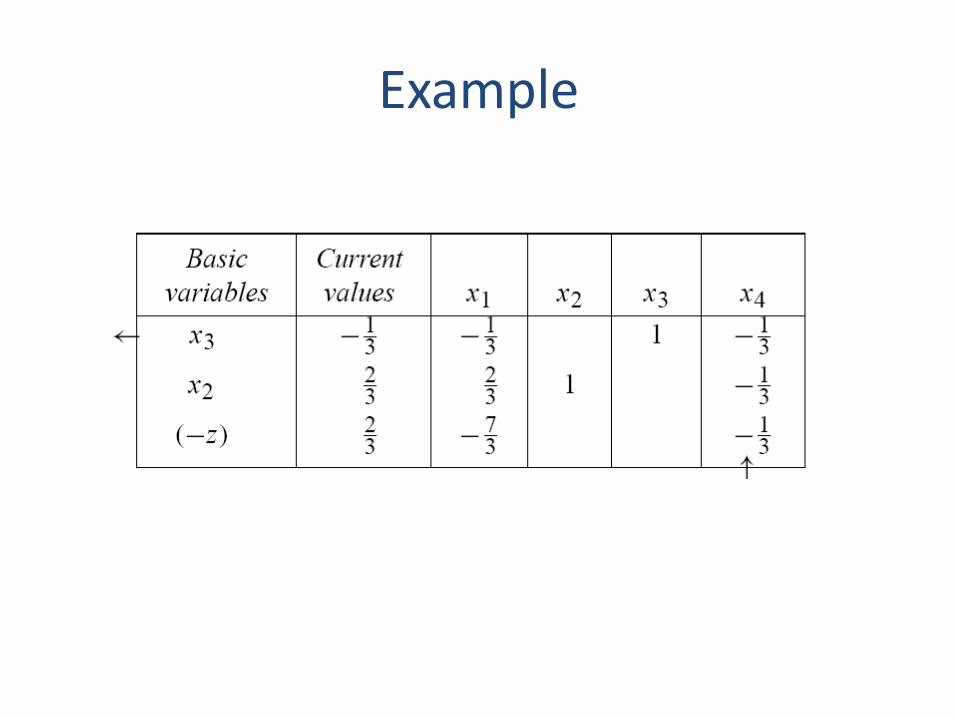
An example of application of the the parametric primal-dual algorithm

• After adding slack variables (canonical form) it is

not feasible, neither primal or dual. • We will consider an arbitrary parameter θ large

enough, so that this system of equations satisfies the primal feasibility and primal optimality conditions.

Example

• Decrease θ until zero, performing the needed iterations, primal or dual, depending on where unfeasibility appears.

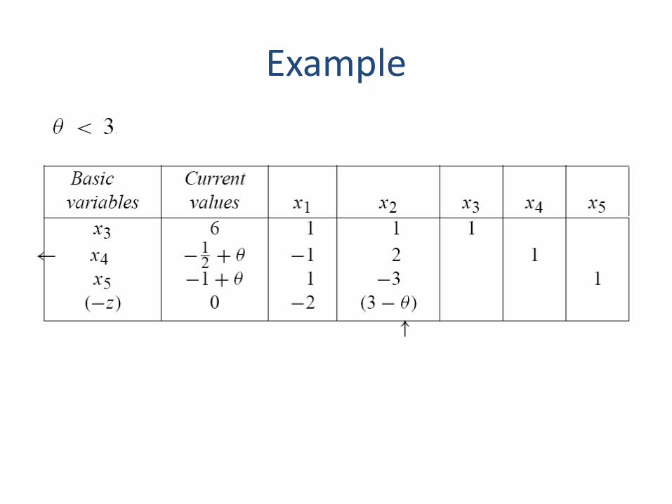
Example

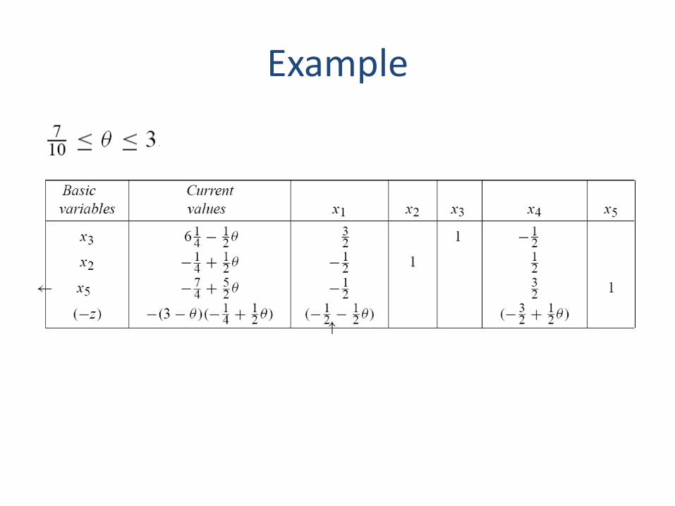
Example

Example

• As we continue to decrease θ to zero, the optimality conditions remain satisfied. Thus the optimal final tableau for this example is given by setting θ equal to zero.

MATHEMATICAL ECONOMICS

The dual as the price-setting mechanism in a perfectly competitive economy

• Suppose that a firm may engage in any n production activities that consume and/or produce m resources in the process.

• Let: – xj ≥ 0 be the level at which the jth activity is operated, – cj be the revenue per unit (minus means cost) generated

from engaging in the jth activity, – aij be the amount of the ith resource consumed (minus

means produced) per unit level of operation of the jth activity.

• Assume that the firm starts with a position of bi units of the ith resource and may buy or sell this resource at a price yi ≥ 0 determined by an external market.

• Since the firm generates revenues and incurs costs by engaging in production activities and by buying and selling resources, its profit is given by:

where the second term includes revenues

from selling excess resources and costs of buying additional resources.

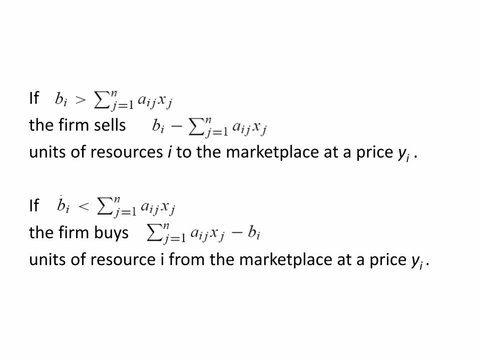
If the firm sells units of resources i to the marketplace at a price yi .

If the firm buys units of resource i from the marketplace at a price yi .

The ‘‘malevolent market"

• The market mechanism for setting prices is such that it tends to minimize the profits of the firm, since these profits are construed to be at the expense of someone else in the market.

• That is, given xj for j = 1, 2, . . . , n, the market reacts to minimize the firm’s profit:

With this market…

• Consuming any resource that needs to be purchased from the marketplace, is clearly uneconomical for the firm, since the market will tend to set the price of the resource arbitrarily high so as to make the firm’s profits arbitrarily small.

• Therefore, the firm will choose to:

• If any resource were not completely consumed by the firm in its own production and therefore became available for sale to the market, this ‘‘malevolent market" would set a price of zero for that resource in order, again, to minimize the firm’s profit.

• Therefore, the profit expression reduces to:

In short, in a ‘‘malevolent market“ the firm’s problem is:

And now the impact of the firm’s decisions on the market…

• Rearranging the profit expression:

Look at the problem from the standpoint of the market…

• If the market sets the prices so that the revenue from engaging in an activity exceeds the market cost, then the firm would be able to make arbitrarily large profits by engaging in the activity at an arbitrarily high level, a clearly unacceptable situation from the standpoint of the market.

• The market instead will always choose to set its prices such that:

• If the market sets the price of a resource so that the revenue from engaging in that activity does not exceed the potential revenue from the sale of the resources directly to the market, then the firm will not engage in that activity at all. In this case, the opportunity cost associated with engaging in the activity is in excess of the revenue produced by engaging in the activity.

• Therefore, the profit expression reduces to:

In short, the market’s “decision” problem, of choosing the prices for the resources so as to minimize the firm’s profit, reduces to:

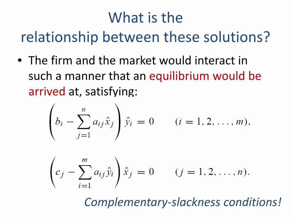
What is the relationship between these solutions? • The firm and the market would interact in

such a manner that an equilibrium would be arrived at, satisfying:

Complementary-slackness conditions!

• If a firm has excess of a particular resource, then the market should not be willing to pay anything for the surplus of that resource since the market wishes to minimize the firm’s profit.

• There may be a nonzero market price on a resource only if the firm is consuming all of that resource that is available.

• Either the amount of excess profit on a given activity is zero or the level of that activity is zero.

• That is, a perfectly competitive market acts to eliminate any excess profits.

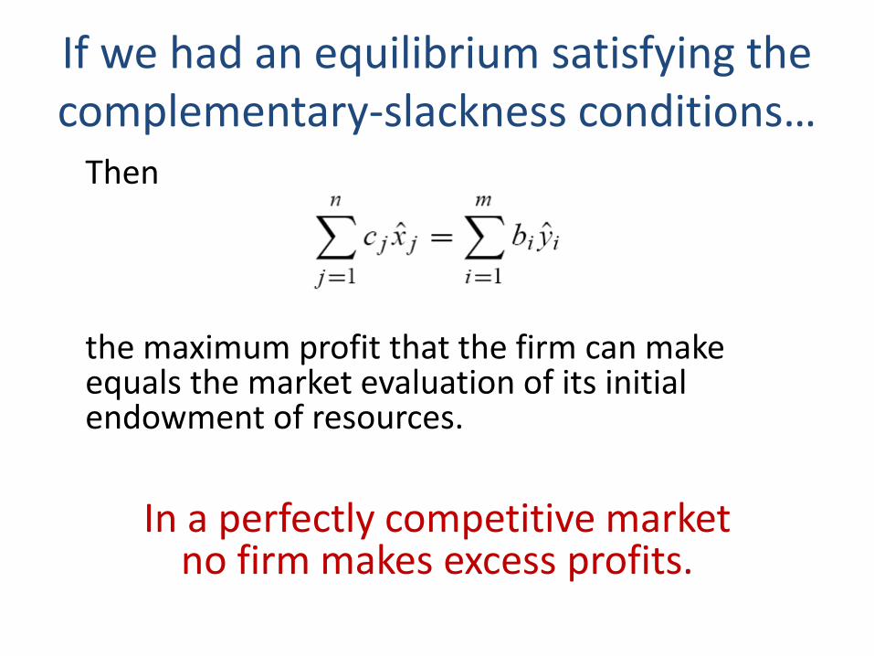
If we had an equilibrium satisfying the complementary-slackness conditions… Then

the maximum profit that the firm can make equals the market evaluation of its initial endowment of resources.

In a perfectly competitive market

no firm makes excess profits.

GAME THEORY

The perfectly competitive economy as a game between the firm and the

malevolent market

• The firm chooses its strategy to maximize its profits while the market behaves (“chooses” its strategy) in such a way as to minimize the firm’s profits.

• Duality theory is, in fact, closely related to game theory.

In many contexts, a decision-maker does not operate in isolation, but in contend with other

decision-makers with conflicting objectives

• Game theory is one approach for dealing with these ‘‘multiperson" decision problems.

• It views the decision-making problem as a game in which each decision-maker, or player, chooses a strategy or an action to be taken.

• When all players have selected a strategy, each individual player receives a payoff.

Example

• There are two players firm R (row player) and firm C (column player).

• The alternatives open to each firm are its advertising possibilities.

• Payoffs are market shares resulting from the combined advertising selections of both firms.

Market share of firm R

• Since we have assumed a two-firm market, firm R and firm C share the market, and firm C receives whatever share of the market R does not.

• Consequently, firm R would like to maximize the payoff entry from the table and firm B would like to minimize this payoff.

Games with this structure are called two-person, zero-sum games. They are zero-sum, since the gain of one player is the loss of the other player.

Behavioral assumptions as to how the players will act

• Both players are conservative, in the sense that they wish to assure themselves of their possible payoff level regardless of the strategy adopted by their opponent.

• It selecting its alternative, firm R chooses a row in the payoff table. The worst that can happen from its viewpoint is for firm C to select the minimum column entry in that row.

Firm R

• If firm R selects its first alternative, then it can be assured of securing 30% of the market.

• If it selects its second alternative it is assured of securing 10%, but no more.

• It will chose alternative 1: maxmin strategy

Firm C

• If firm C selects its first alternative, then it can be assured of losing only 30% of the market, but no more.

• If it selects its second alternative it is assured of losing 40%, but no more.

• If it selects its third alternative it is assured to lose 60%, but no more.

• It will chose alternative 1: minmax strategy

The payoff is the same for both players’ best decision

• The problem has a saddlepoint, an equilibrium solution – Neither player will move unilaterally from this point. – When firm R adheres to alternative 1, then firm C

cannot improve its position by moving to either alternative 2 or 3 since then firm R’s market share increases to either 40% or 60%.

– Similarly, when firm C adheres to alternative 1, then firm R as well will not be induced to move from its saddlepoint alternative, since its market share drops to 20% if it selects alternative 2.

A new payoff table… (firm R market share)

• Given any choice of decisions by the two firms, one of them can always improve its position by changing its strategy.

• If, for instance, both firms choose alternative 1…

And if a player selects a strategy according to some preassigned probabilities,

instead of choosing outright?

• Suppose that firm C selects among its alternatives with probabilities x1, x2, and x3, respectively.

• Then the expected market share of firm R is:

if firm R selects alternative 1, or

• if firm R selects alternative 2.

• Since any gain in market share by firm R is a loss to firm C, firm C wants to make the expected market share of firm R as small as possible.

• Firm C can minimize the maximum expected market share of firm R by solving the following linear program:

• The solution to this linear program is:

with an expected market share for firm R decreasing from 40 percent (minimax strategy payoff) to 35 percent.

Let us now see how firm R might set probabilities y1 and y2 on its alternative

selections to achieve its best security level

• When firm R weights its alternatives by y1 and y2, it has an expected market share of:

• Firm R wants its market share as large as possible, but takes a conservative approach in maximizing its minimum expected market share from these three expressions.

• In this case, firm R solves the following linear program:

• Firm R acts optimally by selecting its first alternative with probability y1 = 5/6 and its second alternative with probability y2 = 1/6 , giving an expected market share of 35 percent.

The security levels resulting from each linear program are identical!

• The linear programming problems are dual of each other (check…).

• Two-person, zero-sum games reduce to primal and dual linear programs!

Historically, game theory was first developed by John von Neumann in 1928 and then helped motivate duality theory in linear programming some twenty years later.