DTAM: Dense Tracking and Mapping in Real-Time

Richard A. Newcombe, Steven J. Lovegrove and Andrew J. DavisonDepartment of Computing, Imperial College London, UK

[rnewcomb,sl203,ajd]@doc.ic.ac.uk

Abstract

DTAM is a system for real-time camera tracking and recon-struction which relies not on feature extraction but dense,every pixel methods. As a single hand-held RGB cameraflies over a static scene, we estimate detailed textured depthmaps at selected keyframes to produce a surface patchworkwith millions of vertices. We use the hundreds of imagesavailable in a video stream to improve the quality of a sim-ple photometric data term, and minimise a global spatiallyregularised energy functional in a novel non-convex opti-misation framework. Interleaved, we track the camera’s6DOF motion precisely by frame-rate whole image align-ment against the entire dense model. Our algorithms arehighly parallelisable throughout and DTAM achieves real-time performance using current commodity GPU hardware.We demonstrate that a dense model permits superior track-ing performance under rapid motion compared to a state ofthe art method using features; and also show the additionalusefulness of the dense model for real-time scene interac-tion in a physics-enhanced augmented reality application.

1. Introduction

Algorithms for real-time SFM (Structure from Motion), aproblem alternatively referred to as Monocular SLAM, havealmost always worked by generating and tracking sparsefeature-based models of the world. However, it is increas-ingly clear that in both reconstruction and tracking it is pos-sible to get more complete, accurate and robust results us-ing dense methods which make use of all of the data inan image. Methods for high quality dense stereo recon-struction from multiple images (e.g. [15, 4]) are becomingreal-time capable due to their high parallelisability, allow-ing them to track the currently dominant GPGPU hardwarecurve. Meanwhile, the first live dense reconstruction sys-

This work was supported by DTA scholarships to R. Newcombe andS. Lovegrove, and ERC Starting Grant 210346. We are very grateful to ourcolleagues at Imperial College London for countless useful discussions.

tems working with a hand-held camera have recently ap-peared (e.g. [9, 13]), but these still rely on feature tracking.

Here we present a new algorithm, DTAM (Dense Trackingand Mapping), which unlike all previous real-time monoc-ular SLAM systems both creates a dense 3D surface modeland immediately uses it for dense camera tracking via wholeimage registration. As a hand-held camera browses a sceneinteractively, a texture-mapped scene model with millionsof vertices is generated. This model is composed of depthmaps built from bundles of frames by dense and sub-pixelaccurate multi-view stereo reconstruction. The reconstruc-tion framework is targeted at our live setting, where hun-dreds of narrow-baseline video frames are the input to eachdepth map. We gather photometric information sequentiallyin a cost volume, and incrementally solve for regulariseddepth maps via a novel non-convex optimisation frameworkwith elements including accelerated exact exhaustive searchto avoid coarse-to-fine warping and the loss of small details,and an interleaved Newton step to achieve fine accuracy.

Meanwhile, in an interleaved fashion, the camera’s pose istracked at frame-rate by whole image alignment against thedense textured model. This tracking benefits from the pre-dictive capabilities of a dense model with regard to occlu-sion handling and multi-scale operation, making it muchmore robust and at least as accurate as any feature-basedmethod; in particular, performance degrades remarkablygracefully in reaction to motion blur or camera defocus.

The limited processing resources imposed by real-timeoperation seemed to preclude dense methods in previousmonocular SLAM systems, and indeed the recent availabil-ity of powerful commodity GPGPU processors is a ma-jor enabler of our approach in both the reconstruction andtracking components. However, we also believe that therehas been a lack of understanding of the power of bring-ing dense methods fully ‘into the loop’ of tracking and re-construction. The availability of a dense scene model, allthe time, enables many simplifications of issues with point-based systems, for instance with regard to multiple scalesand rotations, occlusions or blur due to rapid motion. Also,our view is that the high quality correspondence requiredby both tracking and reconstruction will always be most

robustly and accurately enabled by dense methods, wherematching at every pixel is supported by the totality of dataacross an image and model.

2. Method

The overall structure of our algorithm is straightforward.Given a dense model of the scene, we use dense whole im-age alignment against that model to track camera motionat frame-rate. And tightly interleaved with this, given im-ages from tracked camera poses, we update and expand themodel by building and refining dense textured depth maps.Once bootstrapped, the system is fully self-supporting andno feature-based skeleton or tracking is required.

2.1. Preliminaries

We refer to the pose of a camera c with respect to the worldframe of reference w as

Twc =

(Rwc cw0T 1

), (1)

where Twc ∈ SE(3) is the matrix describing point trans-fer between the camera’s frame of reference and that of theworld, such that xw = Twcxc. Rwc ∈ SO(3) is the ro-tation matrix describing directional transfer, and cw is thelocation of the optic center of camera c in the frame ofreference w. Our camera has fixed and pre-calibrated in-trinsic matrix K and all images are pre-warped to removeradial distortion. We describe perspective projection of a3D point xc = (x, y, z)> including dehomogenisation byπ(xc) = (x/z, y/z)>.

Our dense model is composed of overlapping keyframes. Il-lustrated in Figure 1, a keyframe r with world-camera frametransform Trw, contains an inverse depth map ξr : Ω → Rand RGB reference image Ir : Ω → R3 where Ω ⊂ R2

is the image domain. For a pixel u := (u, v)> ∈ Ω,we can back-project an inverse depth value d = ξ(u) toa 3D point x = π−1(u, d) where π−1(u, d) = 1

dK−1u.The dot notation is used to define the homogeneous vectoru := (u, v, 1)>.

2.2. Dense Mapping

We follow a global energy minimisation framework to es-timate ξr iteratively from any number of short baselineframes m ∈ I(r), where our energy is the sum of a photo-metric error data term and robust spatial regularisation term.We make each keyframe available for use in pose estimationafter initial solution convergence.

We now define a projective photometric cost volume Cr forthe keyframe as illustrated in Figure 1. A row Cr(u) in

Figure 1. A keyframe r consists of a reference image Ir with poseTrw and data cost volume Cr . Each pixel of the reference frameur has an associated row of entries Cr(u) (shown in red) thatstore the average photometric error or cost Cr(u, d) computedfor each inverse depth d ∈ D in the inverse depth range D =[ξmin, ξmax]. We use tens to hundreds of video frames indexed asm ∈ I(r), where I(r) is the set of frames nearby and overlappingr, to compute the values stored in the cost volume.

the cost volume (called a disparity space image in stereomatching [14], and generalised more recently in [10] forany discrete per pixel labelling) stores the accumulated pho-tometric error as a function of inverse depth d. The aver-age photometric error Cr(u, d) is computed by projecting apoint in the volume into each of the overlapping images andsumming the L1 norm of the individual photometric errorsobtained:

Cr(u, d) =1

|I(r)|∑

m∈I(r)

‖ρr (Im,u, d) ‖1 , (2)

where the photometric error for each overlapping image is:

ρr (Im,u, d) = Ir (u)− Im(π(KTmrπ

−1 (u, d))). (3)

Under the brightness constancy assumption, we hope forρ to be smallest at the inverse depth corresponding to thetrue surface. Generally, this does not hold for images cap-tured over a wide baseline and even for the same viewpointwhen lighting changes significantly. Here, rather than usinga patch-based normalised score, or pre-processing the inputdata to increase illumination invariance over wide baselines,we take the opposite approach and show the advantage ofreconstruction from a large number of video frames takenfrom very close viewpoints where very high quality match-ing is possible. We are particularly interested in real-timeapplications where a robot or human is in the reconstruc-tion loop, and so could purposefully restrict the collectionof images to within a relatively narrow region.

In Figure 2, we show plots for three reference pixels wherethe function ρ (Equation 3) has been computed and aver-

Figure 2. Plots for the single pixel photometric functions ρ(u) and the resulting total data cost row C(u) are shown for three examplepixels in the reference frame, chosen in regions of differing discernibility. Pixel (a) is in a textureless region and not well localisable; (b)is within a strongly textured region where a point feature might be detected; and (c) is in a region of linear repeating texture. While theindividual costs exhibit many local minima, the total cost shows clear a clear minimum in all except nearly homogeneous regions.

aged to form C(u) (Equation 2). It is clear that while anindividual data term ρ can have many minima, the total costgenerally has very few and often a clear minimum. Eachsingle ρ is a simple two view stereo data term, and as suchhas no useful information for scene regions which are oc-cluded in the second view. As noted in [13], while increas-ing signal to noise ratio, using many views with a robust L1

norm enables the occlusions to be treated as outliers, whileincreasing the chance that a region has at least one usefulnon occluding data term.

Shown in Figure 3, an inverse depth map can be extractedfrom the cost volume by computing arg mindC(u, d) foreach pixel u in the reference frame. It is clear that the esti-mates obtained in featureless regions are prone to false min-ima. Fortunately, the sum of individual photometric errorsin these regions leads to a flatter total cost. We will there-fore seek an inverse depth map which minimises an energyfunctional comprising the photometric error cost as a dataterm and a regularisation term that penalises deviation froma spatially smooth inverse depth map solution.

2.2.1 Regularised Cost

We assume that the inverse depth solution being recon-structed consists of regions that vary smoothly together withdiscontinuities due to occlusion boundaries. We use a regu-lariser comprising a weighted Huber norm over the gradientof the inverse depth map, g(u)‖∇ξ(u)‖ε. The Huber normis a composite of two convex functions:

‖x‖ε =

‖x‖22

2ε if ‖x‖2 ≤ ε‖x‖1 − ε

2 otherwise(4)

Within ‖∇ξr‖2 ≤ ε an L22 norm is used, promoting smooth

reconstruction, while otherwise the norm is L1 forming thetotal variation (TV) regulariser which allows discontinu-ities to form at depth edges. More specifically, TV allowsdiscontinuities to form without the need for a threshold-specific non-convex norm that would depend on the recon-struction scale which is not available in a monocular setting.

In this case ε is set to a very small value≈ 1.0e−4 to reducethe stair-casing effect obtained by the pure TV regulariser.As depth discontinuities often coincide with edges in thereference image, the per pixel weight g(u) we use is:

g(u) = e−α‖∇Ir(u)‖β2 , (5)

reducing the regularisation strength where the edge mag-nitude is high, thereby limiting solution smoothing acrossregion boundaries. The resulting energy functional there-fore contains a non-convex photometric error data term anda convex regulariser:

Eξ =

∫Ω

g(u)‖∇ξ(u)‖ε + λC (u, ξ(u))

du . (6)

In many optical flow and variational depth map methods,a convex approximation to the data term can be obtainedby linearising the cost volume and solving the resultingapproximation iteratively within a coarse-to-fine warpingscheme that can lead to loss of reconstruction detail. If thelinearisation is performed directly in image space as in [13],all images used in the data term must be kept increasingcomputational cost as more overlapping images are used.Instead, following the large displacement optic flow methodof [12] we approximate the energy functional by couplingthe data and regularisation terms through an auxiliary vari-able α : Ω→ R,

Eξ,α =

∫Ω

g(u)‖∇ξ(u)‖ε +

1

2θ(ξ(u)−α(u))

2

+ λC (u,α(u))

du .

(7)

The coupling term Q(u) = 12θ (ξ(u) − α(u))2 serves to

drive the original and auxiliary variables together, enforc-ing ξ = α as θ → 0, resulting in the original energy(6). As a function of ξ, the convex sum g(u)‖∇ξ(u)‖ε +Q(u) is a small modification of the TV-L2

2 ROF imagedenoising model term [11], and can be efficiently opti-mised using a primal-dual approach [1][16][3]. Also, al-though still non-convex in the auxiliary variable α, each

Figure 3. Incremental cost volume construction; we show the current inverse depth map extracted as the current minimum cost for eachpixel row dmin

u = arg mind C(u, d) as 2, 10 and 30 overlapping images are used in the data term (left). Also shown is the regularisedsolution that we solve to provide each keyframe inverse depth map (4th from left). In comparison to the nearly 300× 103 points estimatedin our keyframe, we show the ≈ 1000 point features used in the same frame for localisation in PTAM ([6]). Estimating camera pose fromsuch a fully dense model enables tracking robustness during rapid camera motion.

Q(u) + λC (u,α(u)) is now trivially point-wise optimis-able and can be solved using an exhaustive search over afinite range of discretely sampled inverse depth values. Thelack of coarse-to-fine warping means that smaller scene de-tails can be correctly picked out from their surroundings.Importantly, the discrete cost volume C, can be computedby keeping the average cost up to date as each overlappingframe from Im∈I(r) arrives removing the need to store im-ages or poses and enabling constant time optimisation forany number of overlapping images.

2.2.2 Discretisation of the Cost Volume and Solution

The discrete cost volume is implemented as an M ×N ×Selement array, where M × N is the reference image res-olution and S is the number of points linearly samplingthe inverse depth range between ξmax and ξmin. Linearsampling in inverse depth leads to a linear sampling alongepipolar lines when computing ρ.

In the next section we will use MN × 1 stacked rasterisedcolumn vector versions of the inverse depth ξ and auxiliaryα variables (see [16] for more details of similar schemes).d is the vector version of ξ; and a is the vector version ofα.We will also use g to denote the MN × 1 constant vectorcontaining the stacked reference image per-pixel weightscomputed by Equation 5 for image weighted regularisation.

2.2.3 Solution

We now detail our iterative minimisation solution for (7).Following [1][16][3], we use duality principles to arrive atthe primal-dual form of g(u)‖∇ξ(u)‖ε +Q(u). Using thevector notation, we replace the weighted Huber regulariser(4) by its conjugate using the Legendre-Fenchel transform,

‖AGd‖ε = arg maxq, ‖q‖2≤1

〈AGd,q〉−δq(q)− ε

2‖q‖22

, (8)

where the matrix multiplicationAd computes the 2MN×1element gradient vector, G = diag(g) is the element-wise

weighting matrix and δq(q) is the indicator function suchthat for each element q, δq(q) = 0 if ‖q‖1 ≤ 1 and other-wise∞.

Replacing the regulariser with the dual form, the saddle-point problem in primal variable d and dual variable q iscoupled with the data term giving the sum of convex andnon-convex functions we minimise,

arg maxq, ‖q‖2≤1

arg mind,a

E (d,a,q) (9)

E (d,a,q) =〈AGd,q〉+ 1

2θ‖d− a‖22

+λC (a)− δq(q)− ε

2‖q‖22

.

(10)Fixing the auxillary variable a, the condition of optimalityis met when ∂d,q(E (d,a,q)) = 0. For the dual variable q,

∂E (d,a,q)

∂q= AGd− εq . (11)

Using the divergence theorem, differentiation with respectto primal variable d can be performed by noting that〈AGd,q〉 =

⟨A>q, Gd

⟩, where A> forms the negative

divergence operator,

∂E (d,a,q)

∂d= GA>q +

1

θ(d− a) . (12)

For a fixed value d we obtain the solution for each au =a(u) ∈ D in the remaining non-convex function using apoint-wise search to solve,

arg minau∈D

Eaux(u, du, au) , (13)

Eaux(u, du, au) =1

2θ(du − au)

2+ λC (u, au) . (14)

The complete optimisation starting at iteration n = 0 be-gins by setting dual variable q0 = 0 and initialising eachelement of the primal variable with the data cost minimum,d0u = a0

u = arg minau∈D C(u, au), iterating:

Figure 4. Accelerated exhaustive search: at each pixel we wish to minimise the total depth energy Eaux(u) (green), which is the sum ofthe fixed data energy C(u) (red) and the current convex coupling between primal and auxiliary variables Q(u) (blue). This latter term is aparabola which gets narrower as optimisation progresses, setting a bound on the region within which a minimum of Eaux(u) can possiblylie and allowing the search region (unshaded) to get smaller and smaller.

1. Fixing the current value of an perform a semi-implicitgradient ascent on ∂q = 0 (11) and descent on ∂d = 0(12) :

qn+1−qnσq

= AGdn − εqn+1

dn+1−dnσd

= − 1θn

(dn+1 − an

)−GA>qn+1,

resulting in the following primal-dual update step,

qn+1 = Πq ((qn + σqGAdn)/(1 + σqε)) ,

dn+1 = (dn+σd(GA>qn+1+ 1θn a

n))/(1+ σd

θn )

where Πq(x) = x/max(1, ‖x‖2) projects the gradientascent step back onto the constraint ‖q‖1 ≤ 1.

2. Fixing dn+1, perform a point-wise exhaustive searchfor each an+1

u ∈ D (13).

3. If θn > θend update θn+1 = θn (1− βn), n← n+ 1and goto (1), otherwise end.

In practice, the update steps for qn+1 and dn+1 can be per-formed efficiently and in parallel on modern GPU hardwareusing equivalent in-place computations for operators ∇ and−∇· in place of the matrix-vector multiplication involvingA and A>.

2.2.4 Accelerating the Non-Convex Solution

The exhaustive search over all S samples of Q to solve (13)ensures global optimality of the iteration (within the sam-pling limit). We now demonstrate in Figure 4 that thereexists a deterministically decreasing feasible region withinwhich the global minimum of (14) must exist, considerablyreducing the number of samples that need to be tested.

For a pixel u, the known data cost minimum and maximumare Cmaxu = C(dmaxu ) and Cminu = C(dminu ). These aretrivial to maintain when building the cost volume. As both

terms in (14) are positive, we know that the minimum valueof any cost volume row is just Cminu . This occurs if thequadratic component is zero when an+1

u = dn+1u = dminu .

In any case, if we set an+1u = dn+1

u then we can not exceedCmaxu resulting in the energy bound,

Cminu +1

2θn(an+1u − dn+1

u

)2 ≤ Cmaxu (15)

Rearranging for an+1u we find a feasible region either side

of the current fixed point dn+1u within which the solution of

the optimisation must exist,

an+1u ∈

[dn+1u − rn+1

u , dn+1u + rn+1

u

](16)

rn+1u = 2θnλ

(Cmaxu − Cminu

)(17)

As shown in Figure (4), the search region size drasticallydecreases after only a small number of iterations, reducingthe number of sample points that need to be tested in thecost volume to ensure optimally of (13).

2.2.5 Increasing Solution Accuracy

In the large displacement optical flow method of [12] anincreased sampling density of the cost function is used toachieve sub-pixel flows. Likewise, it is possible to increasethe density of inverse depth samples S to increase surfacereconstruction accuracy and the acceleration method intro-duced in the previous section would go a long way to mit-igating the increased computational cost. However, as canbe seen in Figure 4 the sampled point-wise energy Q(u) istypically well modelled around the discrete minimum witha parabola. We can therefore achieve sub-sample accuracyby performing a single Newton step using numerical deriva-tives of Q(u) around the current discrete minimium an+1

u ,

an+1u = an+1

u − ∇Eaux(u, dn+1u , an+1

u )

∇2Eaux(u, dn+1u , an+1

u ). (18)

(a) (b) (c) (d)

(e)

Figure 5. Example inverse depth map reconstructions obtained from DTAM using a single low sample cost volume with S = 32. (a)Regularised solution obtained without the sub-sample refinement is shown as a 3D mesh model with Phong shading (inverse depth mapsolution shown in inset). (b) Regularised solution with sub-sample refinement using the same cost volume also shown as a 3D mesh model.(c) The video frame as used in PTAM, with the point model projections of features found in the current frame and used in tracking. (d,e)Novel wide baseline texture mapped views of the reconstructed scene used for tracking in DTAM.

The refinement step is embedded in the iterative optimisa-tion scheme by replacing the located an+1

u with the sub-sample accurate version. It is not possible to perform thisrefinement post-optimisation, as at that point the quadraticcoupling energy is large (due to a very small θ), and sothe fitted parabola is a spike situated at the minimum. Asdemonstrated in Figure 5 embedding the refinement step in-side each iteration results in vastly increased reconstructionquality, and enables detailed reconstructions even for lowsample rates, e.g. S ≤ 64.

2.2.6 Setting Parameter Values and Post Processing

Gradient ascent/descent time-steps σq, σd are set optimallyfor the update scheme provided as detailed in [3]. Variousvalues of β can be used to drive θ towards 0 as iterations in-crease while ensuring θn+1 < θn (1− βn). Larger valuesresult in lower quality reconstructions, while smaller valuesof β with increased iterations result in higher quality. In ourexperiments we have set β = 0.001 while θn ≥ 0.001 elseβ = 0.0001 resulting in a faster initial convergence. Weuse θ0 = 0.2 and θend = 1.0e − 4. λ should reflect thedata term quality and is set dynamically to 1/(1 + 0.5d),where d is the minimum scene depth predicted by the cur-rent scene model. For the first key-frame we set λ = 1. Thisdynamically altered data term weighting sensibly increasesregularisation power for more distant scene reconstructionsthat, assuming similar camera motions for both closer andfurther scenes, will have a poorer quality data term.

Finally, we note that optimisation iterations can be inter-leaved with updating the cost volume average, enabling thesurface (though in a non fully converged state) to be madeavailable for use in tracking after only a single ρ computa-tion. For use in tracking, we compute a triangle mesh fromthe inverse depth map, culling oblique edges as described in[9].

2.3. Dense Tracking

Given a dense model consisting of one or more keyframes,we can synthesise realistic novel views over wide baselinesby projecting the entire model into a virtual camera. Sincesuch a model is maintained live, we benefit from a fully pre-dictive surface representation, handling occluded regionsand back faces naturally. We estimate the pose of a livecamera by finding the parameters of motion which generatea synthetic view which best matches the live video image.

We refine the live camera pose in two stages; first witha constrained inter-frame rotation estimation, and secondwith an accurate 6DOF full pose refinement against themodel. Both are formulated as iterative Lucas-Kanade stylenon-linear least-squares problems, iteratively minimisingan every-pixel photometric cost function. To converge tothe global minimum, we must initialise the system withinthe convex basin of the true solution. We use a coarse-finestrategy over a power of two image pyramid for efficiencyand to increase our range of convergence.

2.3.1 Pose Estimation

We first follow the alignment method of [8] between con-secutive frames to obtain rotational odometry at lower levelswithin the pyramid, offering resilience to motion blur sinceconsecutive images are similarly blurred. This optimisa-tion is more stable than 6DOF estimation when the numberof pixels considered is low, helping to converge for largepixel motions, even when the true rotation is not strictly ro-tational (Figure 6). A similar step is performed before fea-ture matching in PTAM’s tracker, computing first the inter-frame 2D image transform and fitting a 3D rotation [7].

The rotation estimate helps inform our current best estimateof the live camera pose, Twl. We project the dense modelin to a virtual camera v at location Twv = Twl, with colour

Figure 6. MSE convergence plots over time for an illustrativetracking step using different combinations of rotation and full poseiterations. Estimating rotation first can help to avoid local minima.

image Iv and inverse depth image ξv . Assuming that v isclose to the true pose of the live camera, we perform a 2.5Dalignment between Iv and the live image Il to estimate Tlv,and hence the true pose Twl = TwvTvl. We parametrise anupdate to Tvl by ψ ∈ R6 belonging to the Lie Algebra se3and define a forward-compositional [2] cost function relat-ing photometric error to changing parameters:

F (ψ) =1

2

∑u∈Ω

(fu (ψ)

)2

=1

2‖f(ψ)‖22, (19)

fu(ψ) = Il(π(KTlv(ψ)π−1 (u, ξv (u))

))− Iv (u) (20)

Tlv(ψ) = exp

(6∑i=1

ψigeniSE(3)

). (21)

This cost function does not take into account occluded sur-faces directly; instead we assume that the optimisation op-erates over only a narrow baseline from the original modelprediction. We could perform a full prediction settingTwv = Twl at every iteration but find it is not required.

ψ = arg minψ F (ψ) represents a stationary point ofF (ψ) such that ∇F (ψ) = 0. We approximate F (ψ)

with F (ψ) = 12 f(ψ)>f(ψ) where f(ψ) ≈ f(ψ) is the

Taylor series expansion of f(ψ) about 0 up to first order.Via the product rule, ∇F (ψ) = ∇f(ψ)>f(ψ) and wecan find the approximate minimiser ψ ≈ ψ by solving∇f(ψ)>f(ψ) = 0. Equivalently, we can solve the overde-termined linear system ∇f(0)ψ = −f(0) or its normalequations. We then apply the update Tlv ← TlvT(ψ) andrepeat until ψ ≈ 0 marking convergence.

2.3.2 Robustified Tracking

Any observed pixels which do not belong to our modelmay have a large impact on tracking quality. We robus-tify our method by disregarding pixels whose photometricerror falls above some threshold. In each least squares it-eration, our coarse-fine method ramps down this thresholdas we converge to achieve greater accuracy. This schememakes it practical to track densely whilst observing unmod-elled objects.

Figure 7. Augmented Reality car appears fixed rigidly to the worldas an unmodelled hand is waved in front of the camera. Pixels ingreen are used for tracking whilst blue do not exist in the originalprediction and yellow are rejected (hand / monitor / shadow).

Figure 8. DTAM tracking throughout camera defocus.

2.4. Model Initialisation and Management

The system is initialised using a standard point fea-ture based stereo method, which continues until the firstkeyframe is acquired, when we switch to a fully dense track-ing and mapping pipeline. We are investigating a fully gen-eral dense initialisation scheme.

A new keyframe is added when the number of pixels in theprevious predicted image without visible surface informa-tion falls below some threshold. This is possible due tothe fully dense nature of the system and is arguably betterfounded than the heuristics used in feature based systems.

3. Evaluation

We have evaluated DTAM in the same desktop settingwhere PTAM has been successful. In all experiments, wehave used a Point Grey Flea2 camera, operating at 30Hzwith 640×480 resolution and 24bit RGB colour. The cam-era has pre-calibrated intrinsics. We run on a commoditysystem consisting of an NVIDIA GTX 480 GPU hostedby an i7 quad-core CPU. We present a qualitative compari-son of the live running system including extensive trackingcomparisons with PTAM and augmented reality demonstra-tions in an accompanying video:http://youtu.be/Df9WhgibCQA.

3.1. Quantitative Tracking Performance

We have evaluated the tracking performance of our systemagainst the openly available PTAM system, which includes

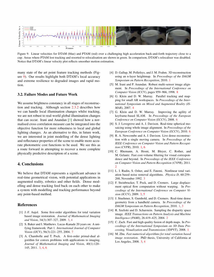
Figure 9. Linear velocities for DTAM (blue) and PTAM (red) over a challenging high acceleration back-and-forth trajectory close to acup. Areas where PTAM lost tracking and resorted to relocalisation are shown in green. In comparison, DTAM’s relocaliser was disabled.Notice that DTAM’s linear velocity plot reflects smoother motion estimation.

many state of the art point feature tracking methods (Fig-ure 9). Our results highlight both DTAM’s local accuracyand extreme resilience to degraded images and rapid mo-tion.

3.2. Failure Modes and Future Work

We assume brightness constancy in all stages of reconstruc-tion and tracking. Although section 2.3.2 describes howwe can handle local illumination changes whilst tracking,we are not robust to real-world global illumination changesthat can occur. Irani and Anandan [5] showed how a nor-malised cross correlation measure can be integrated into theobjective function for more robustness to local and globallighting changes. As an alternative to this, in future work,we are interested in joint modelling of the dense lightingand reflectance properties of the scene to enable more accu-rate photometric cost functions to be used. We see this asa route forward in attempting to recover a more completephysically predictive description of a scene.

4. Conclusions

We believe that DTAM represents a significant advance inreal-time geometrical vision, with potential applications inaugmented reality, robotics and other fields. Dense mod-elling and dense tracking feed back on each other to makea system with modelling and tracking performance beyondany point-based method.

References

[1] J.-F. Aujol. Some first-order algorithms for total variationbased image restoration. Journal of Mathematical Imagingand Vision, 34(3):307–327, 2009. 3, 4

[2] S. Baker and I. Matthews. Lucas-Kanade 20 years on: A uni-fying framework: Part 1. International Journal of ComputerVision (IJCV), 56(3):221–255, 2004. 7

[3] A. Chambolle and T. Pock. A first-order primal-dual al-gorithm for convex problems with applications to imaging.Journal of Mathematical Imaging and Vision, 40(1):120–145, 2011. 3, 4, 6

[4] D. Gallup, M. Pollefeys, and J. M. Frahm. 3D reconstructionusing an n-layer heightmap. In Proceedings of the DAGMSymposium on Pattern Recognition, 2010. 1

[5] M. Irani and P. Anandan. Robust multi-sensor image align-ment. In Proceedings of the International Conference onComputer Vision (ICCV), pages 959–966, 1998. 8

[6] G. Klein and D. W. Murray. Parallel tracking and map-ping for small AR workspaces. In Proceedings of the Inter-national Symposium on Mixed and Augmented Reality (IS-MAR), 2007. 4

[7] G. Klein and D. W. Murray. Improving the agility ofkeyframe-based SLAM. In Proceedings of the EuropeanConference on Computer Vision (ECCV), 2008. 6

[8] S. J. Lovegrove and A. J. Davison. Real-time spherical mo-saicing using whole image alignment. In Proceedings of theEuropean Conference on Computer Vision (ECCV), 2010. 6

[9] R. A. Newcombe and A. J. Davison. Live dense reconstruc-tion with a single moving camera. In Proceedings of theIEEE Conference on Computer Vision and Pattern Recogni-tion (CVPR), 2010. 1, 6

[10] C. Rhemann, A. Hosni, M. Bleyer, C. Rother, andM. Gelautz. Fast cost-volume filtering for visual correspon-dence and beyond. In Proceedings of the IEEE Conferenceon Computer Vision and Pattern Recognition (CVPR), 2011.2

[11] L. I. Rudin, S. Osher, and E. Fatemi. Nonlinear total vari-ation based noise removal algorithms. Physica D, 60:259–268, November 1992. 3

[12] F. Steinbrucker, T. Pock, and D. Cremers. Large displace-ment optical flow computation without warping. In Pro-ceedings of the International Conference on Computer Vi-sion (ICCV), 2009. 3, 5

[13] J. Stuehmer, S. Gumhold, and D. Cremers. Real-time densegeometry from a handheld camera. In Proceedings of theDAGM Symposium on Pattern Recognition, 2010. 1, 3

[14] R. Szeliski and D. Scharstein. Sampling the disparity spaceimage. IEEE Transactions on Pattern Analysis and MachineIntelligence (PAMI), 26:419–425, 2004. 2

[15] C. Zach. Fast and high quality fusion of depth maps. In Pro-ceedings of the International Symposium on 3D Data Pro-cessing, Visualization and Transmission (3DPVT), 2008. 1

[16] M. Zhu. Fast numerical algorithms for total variation basedimage restoration. PhD thesis, University of California atLos Angeles, 2008. 3, 4