dsc-ritz method for the free vibration analysis of mindlin plates

INTERNATIONAL JOURNAL FOR NUMERICAL METHODS IN ENGINEERINGInt. J. Numer. Meth. Engng 2005; 62:262–288Published online 8 November 2004 in Wiley InterScience (www.interscience.wiley.com). DOI: 10.1002/nme.1186

DSC-Ritz method for the free vibration analysis of Mindlin plates

Yunshan Hou1, G. W. Wei2,3,∗,† and Y. Xiang4

1Department of Computational Science, National University of Singapore, Singapore 1175432Department of Mathematics, Michigan State University, East Lansing, MI 48824, U.S.A.

3Department of Electrical and Computer Engineering, Michigan State University, East Lansing,

MI 48824, U.S.A.4School of Engineering and Industrial Design and Centre for Construction Technology and Research,

University of Western Sydney, Penrith South DC, NSW 1797, Australia

SUMMARY

This paper introduces a novel method for the free vibration analysis of Mindlin plates. The proposedmethod takes the advantage of both the local bases of the discrete singular convolution (DSC)algorithm and the pb-2 Ritz boundary functions to arrive at a new approach, called DSC-Ritz method.Two basis functions are constructed by using DSC delta sequence kernels of the positive type. Theenergy functional of the Mindlin plate is represented by the newly constructed basis functions andis minimized under the Ritz variational principle. Extensive numerical experiments are consideredby different combinations of boundary conditions of Mindlin plates of rectangular and triangularshapes. The performance of the proposed method is carefully validated by convergence analysis. Thefrequency parameters agree very well with those in the literature. Numerical experiments indicate thatthe proposed DSC-Ritz method is a very promising new method for vibration analysis of Mindlinplates. Copyright � 2004 John Wiley & Sons, Ltd.

KEY WORDS: DSC kernel; Ritz method; meshless method; Mindlin plate theory; vibration analysis

1. INTRODUCTION

Plates are some of the most important structural elements and its theoretical descriptions wereestablished by Chladni [1] and Kirchhoff [2]. The classical thin (Kirchhoff) plate theory haslimited success for thick plates because no account is taken for the effect of transverse sheardeformation on the mechanical behaviour of thick plates [3]. To allow for this effect, Mindlin [4]proposed a simple model by assuming a constant transverse shear–strain distribution through theplate thickness. Analytical solution to Mindlin plates is scarce [5, 6], and numerical computationsare indispensable for obtaining approximate solutions that are important in engineering practices.

Typically, structural computations are accomplished by using either global methods orlocal methods. Global methods, such as the Rayleigh method [7], Ritz methods [8–14], series

∗Correspondence to: G. W. Wei, Department of Mathematics, Michigan State University, East Lansing, MI 48824,U.S.A.

†E-mail: [email protected] Received 23 April 2003Revised 16 January 2004

Copyright � 2004 John Wiley & Sons, Ltd. Accepted 7 May 2004

DSC-RITZ METHOD FOR THE FREE VIBRATION ANALYSIS 263

expansion [15], methods of differential quadrature [16] and generalized differential quadrature[17, 18], etc, are highly accurate but are often cumbersome to implement in dealing with com-plex geometries and non-conventional boundary conditions. In contrast, local methods, such asfinite strip methods [19] and spline finite strip methods [20], are easy to implement for complexgeometries and discontinuous boundary conditions. However, the accuracy of local methods isrelatively low compared to that of global methods. As point out by Zienkiewicz, local methodsmight converge slowly and are too expensive for the prediction of short waves (i.e., high-ordereigenmodes) [21].

Recently, the discrete singular convolution (DSC) algorithm [22] has emerged as a novelapproach that exhibits global methods’ accuracy for integration and local methods’ flexibilityfor handling complex geometries and boundary conditions. The mathematical foundation ofthe DSC algorithm is the theory of distributions and wavelet analysis. The same theory alsounderpins the basis for singular transforms of Hilbert type, Abel type and delta type. Thesetransforms have important applications to analytical signal processing, tomography and sur-face interpolation. Numerical solutions to differential equations are formulated via the singularkernels of the delta type. Based on the DSC framework, a unification was discussed for anumber of conventional computational methods, including global, local, Galerkin, collocation,and finite difference methods [23, 24].

The DSC algorithm has found its success in fluid dynamic simulation [25] and electromag-netic wave propagation [26]. One of the most successful applications that the DSC algorithmhas accomplished so far is the analysis of solid structures [24, 27–35]. The DSC algorithm wasutilized to provide at least 11 significant digits for the first 100 modes of a simply supportedsquare plate governed by the fourth-order biharmonic equations [27]. The DSC algorithm hasbeen used for vibration analysis of plates with simply supported, clamped, and transverselysupported edges [33], mixed edge supports [30], complex internal supports [24, 32], irregu-lar internal supports [35], and plates subjected to high-frequency vibration levels [31, 34]. Inparticular, analysis of plates with irregular supports is a challenging task because of possi-ble ill-conditioned matrix. Analysis of high-frequency vibration modes is another challengingproblem in structural design [21]. Low-order methods, like h-version finite element methods,converge slowly for high-order modes. Standard global methods fail to work for high-ordermodes due to the numerical round off errors when the degree of polynomial is increased to acertain level. The DSC algorithm provides accurate prediction of thousands of vibration modes,which was not available to engineers previously [31, 34].

Another distinct development in numerical analysis of plates is the pb-2 Rayleigh–Ritzmethod [36, 37]. The method avoids the difficulty of global methods for implementing bound-ary conditions by appropriately choosing the basis function so that the boundary conditionsare automatically satisfied. Essentially, the product of a two-dimensional polynomial function(p-2) and a boundary function (b) is utilized. The boundary function constitutes proper powersof polynomials that are simultaneous solutions to the differential equations of the boundaryconditions. In the past decade, the pb-2 Rayleigh–Ritz method has had substantial success in thevibration analysis of Mindlin plates [37–43]. Much advance in this direction was summarizedin a monograph [36].

The objective of the present work is to explore a new computational method, which is acombination of the DSC algorithm and pb-2 Rayleigh–Ritz method, and thus, called DSC-Ritzmethod. The essential idea is to utilize the local DSC approximations and the pb-2 Rayleigh–Ritz boundary functions. As a result, the DSC-Ritz method has the advantage of both methods.

Copyright � 2004 John Wiley & Sons, Ltd. Int. J. Numer. Meth. Engng 2005; 62:262–288

264 Y. HOU, G. W. WEI AND Y. XIANG

The method was proposed and tested on vibration analysis of beams and thin plates by twoof the present authors [44]. This paper further investigates the efficiency and convergence ofthe DSC-Ritz method for the vibration analysis of Mindlin plates.

Albeit the proposed DSC-Ritz method has a distinct mathematical foundation, it sharessome similarities with the smooth particle hydrodynamics [45, 46], meshless method [47], andelement-free kp-Ritz method [48, 49]. The latter makes use of the cubic spline function toconstruct the shape function and the penalty method to enforce essential boundary conditions.Such similarities enhance our understanding of the philosophy of both the previous meshlesstype of methods and the DSC-Ritz.

The organization of this paper is as follows. Section 2 is devoted to theoretical formulations.The philosophy of the DSC algorithm is briefly discussed. The energy formulation of Mindlinplates is described. Detailed boundary conditions are given and the DSC-Ritz formalism ispresented with two sets of new basis functions. In Section 3, the new method are applied tothe numerical analysis of Mindlin plates with different shapes and combinations of boundaryconditions. Validation is conducted by extensive convergence study and by a comparison withthe literature. This paper ends with a conclusion.

2. THEORETICAL FORMULATIONS

In this section, a brief review is given to the theory of DSC before the formalism of Mindlinplates is described. The DSC-Ritz method of solution is introduced in the last subsection.

2.1. Discrete singular convolution

Singular convolutions occur commonly in many science and engineering problems and area special class of mathematical transformations. It is most convenient to discuss singularconvolutions in the context of the theory of distributions. The latter has a significant impact inmathematical analysis. It provides a rigorous justification for a number of informal manipulationsin engineering and has significant influence over many mathematical disciplines, such as operatorcalculus, differential equations, functional analysis, harmonic analysis, harmonic analysis andtransformation theory. Let T be a distribution and �(t) be an element of the space of testfunctions. A singular convolution can be defined as

F(t) = (T �)(t) =∫ ∞

−∞T (t − x)�(x) dx (1)

Here T (t − x) is a singular kernel. Depending on the form of the kernel T , the singularconvolution is the key issue for a wide range of science and engineering problems, such asHilbert transform, Abel transform and Radon transform. In the present study, only the singularkernels of the delta type are required

T (x) = �(n)(x), (n = 0, 1, 2, . . .) (2)

Here, kernel T (x) = �(x) is the delta distribution and is of particular importance for interpo-lation of surfaces and curves. Higher-order kernels, T (x) = �(n), (n = 1, 2, . . .) are essentialfor numerically solving differential equations and for image processing, noise estimation, etc.However since these kernels are very singular, they cannot be directly digitized in computers.



Hence, the singular convolution, (1), is of little direct numerical merit. To avoid the difficultyof using singular expressions directly in computer, we construct sequences of approximations(T�) to the distribution T

lim�→�0

T�(x) → T (x) (3)

where �0 is a generalized limit. Obviously, in the case of T (x) = �(x), each element in thesequence, T�(x), is a delta sequence kernel. With a sufficiently smooth approximation, it isuseful to consider a discrete singular convolution

F�(t) =∑k

T�(t − xk)f (xk) (4)

where F�(t) is an approximation to F(t) and {xk} is an appropriate set of discrete points onwhich the DSC (4) is well defined. Note that, the original test function �(x) has been replacedby f (x).

Obviously, as the Fourier transform of the delta distribution is unit in the Fourier domain,the distribution can be regarded as a universal reproducing kernel [22]

f (x) =∫

�(x − x′)f (x′) dx′ (5)

As a consequence, delta sequence kernels are approximate reproducing kernels or bandlimitedreproducing kernels which provide good approximation to the universal reproducing kernel incertain frequency bands.

There are many delta sequence kernels arising in the theory of partial differential equations,Fourier transforms and signal analysis, with completely different mathematical properties. Thereader is referred to References [22, 24] for an elaboration on historical aspects of the deltadistribution and its approximations. For the purpose of numerical computations, the delta se-quence kernels of both positive type and Dirichlet type are of particular importance and havevery distinct mathematical and numerical properties.

DefinitionLet {��} be a sequence of kernel functions on (−∞, ∞) which are integrable over everybounded interval. We call {��} a delta sequence kernel of positive type if

1.∫ a

−a�� → 1 as � → �0 for some finite constant a.

2. For every constant � > 0,(∫ −�

−∞ + ∫∞�

)�� → 0 as � → �0.

3. ��(x) � 0 for all x and �.

Although the delta sequence kernels of Dirichlet type have been extensively studied in ourprevious numerical work in the framework of the collocation, use of delta sequence kernelsof positive type has rarely been considered. However, a variety of delta sequence kernelsof positive type were described in detail in Reference [24]. Important examples include im-pulse functions, Gauss’ delta sequence kernel, Lorentz’s delta sequence kernel, Landau’s deltasequence kernel, Poisson’s delta sequence kernel family, Fejér’s delta sequence kernel and itsgeneralization. Most of these kernels were utilized in our previous test [44]. In this work, we



x, ξ

b

y, η

a

Figure 1. Geometry of rectangular Mindlin plate.

focus our study on two typical kernels, Gauss’ delta sequence kernel

��(x) = 1√2��

e−x2/2�2(6)

and Fejer’s delta sequence kernel

�k(x) ={

Fk(x) |x| � �, k = 0, 1, 2 . . .

0 otherwise(7)

where

Fk(x) = sin2( 1

2 kx)

2�k sin2( 1

2 x) , −∞ < x < ∞ (8)

A major advantage of many DSC delta sequence kernels is their localization. For example, theGauss’ kernel is an element of the Schwartz space functions. The decay property of the Fejer’skernel can be improved by choosing appropriate parameter �. It was well understood that the useof delta sequence kernels of positive type has to be formulated in a Galerkin algorithm [23].For conservative systems, such as vibration of plates, the Galerkin algorithm is essentiallyidentical to the Ritz variational formulation. Thus, the rest of this section is devoted to theseissues.

2.2. Energy functionals of Mindlin plates

In this subsection, we briefly review the theory of Mindlin plates to establish concepts andnotations. More detailed description can be found elsewhere [40]. Let us consider a flat,isotropic, thick, rectangular (or triangular) plate of uniform thickness h, length a, width b,Young’s modulus E, shear modulus G and Poisson’s ratio �. The geometry of a rectangularplate is shown in Figure 1. The plate may have an arbitrary combination of different supportingedges. The goal is to determine the natural frequencies of the plate.

According to the first-order shear deformable plate theory [4], the displacement fields of theplate in orthogonal co-ordinates can be expressed as

u(x, y, z) = z�x(x, y), v(x, y, z) = z�y(x, y), w(x, y, z) = w(x, y) (9)



where u, v are inplane displacements in the x-, and y-directions, respectively, w the transversedisplacement, and �x(x, y) and �y(x, y) the bending slopes along the y- and x-axes, respectively.Note that �x and �y depend on variables x and y, and the transverse displacement, w, is assumedto be independent of z, i.e. no thickness deformation is allowed. In view of Equation (9) andusing Green’s definition for strains,

� = {εxx, εyy, �xy, �xz, �yz}T ={

�u

�x,

�v

�y,

�u

�y+ �v

�x,

�u

�z+ �w

�x,

�v

�z+ �w

�y

}T

(10)

where � is the strain tensor having various non-vanishing components described in Equation (10).To construct the energy functional, we consider the strain energy functional of the plate [40]

U = 1

2

∫V

�T[B]� dV (11)

where V is the volume of the plate, and [B] a matrix determined by material property and isgiven by

[B] =

E

1 − �2

�E

1 − �2 0 0 0

�E

1 − �2

E

1 − �2 0 0 0

0 0 G 0 0

0 0 0 G 0

0 0 0 0 G

(12)

where G = E/[2(1+�)] and is the shear correction factor that is used to compensate the errordue to the assumption of constant transverse shear strain distribution over the plate thicknessin the Mindlin plate theory.

The strain energy, Equation (11), can be evaluated from Equations (9), (10) and (12) to yield

U = 1

2

∫V

{Ez2

1 − �2

[(��x

�x+ ��y

�y

)2− 2(1 − �)

(��x

�x

��y

�y− 1

4

(��x

�y+ ��y

�x

)2)]

+G

[(�x + �w

�x

)2+(

�y + �w

�y

)2]}dV (13)

As expected, the well-known strain energy for thin plates can be obtained if we set �x =−�w/�x and �y = −�w/�y in Equation (13).

Another important component in the energy functional is the kinetic energy T . For freevibration, the kinetic energy for the plate is given by T = 1

22∫A[�hw2 + 1

12�h3(�2x +�2

y)] dA,where is the angular frequency and � the mass density of the plate.

It is well-known that the total energy functional can be expressed as the difference of thestrain and kinetic energy � = U −T . The latter can be used as the starting point for numericalcomputations.



Table I. Convergence study for rectangular plates with CCCC boundary conditions.

Number Mode sequence numberParameter of grid

a/b h/b Kernel of kernel points 1 2 3 4 5 6

1.0 0.1 Gauss r = 1.8 N = 2 5.1701 11.7620 11.7620 15.8121 67.0104 67.0104N = 4 3.3116 6.3073 6.3073 8.8231 13.2954 13.4748N = 6 3.2984 6.2891 6.2891 8.8145 10.3843 10.4813N = 7 3.2959 6.2884 6.2884 8.8169 10.3803 10.4789N = 8 3.2963 6.2868 6.2868 8.8113 10.3815 10.4800N = 9 3.2956 6.2867 6.2867 8.8122 10.3794 10.4783

Fejer k = 2, r = 3.0 N = 2 5.0659 11.6873 11.6873 15.7348 67.0056 67.0056N = 4 3.3261 6.3049 6.3049 8.8273 12.7812 12.9637N = 6 3.2994 6.2896 6.2896 8.8148 10.3856 10.4824N = 7 3.2958 6.2881 6.2881 8.8163 10.3800 10.4788N = 8 3.2959 6.2864 6.2864 8.8105 10.3805 10.4790N = 9 3.2954 6.2861 6.2861 8.8109 10.3789 10.4780

Reference [50] — — 3.2954 6.2858 6.2858 8.8098 10.3788 10.47780.2 Gauss r = 1.8 N = 2 3.0967 6.0297 6.0297 7.9581 17.7249 17.7249

N = 4 2.6913 4.6967 4.6967 6.3031 7.8131 7.9568N = 6 2.6881 4.6913 4.6913 6.2991 7.1775 7.2765N = 7 2.6876 4.6911 4.6911 6.2994 7.1768 7.2761N = 8 2.6876 4.6909 4.6909 6.2987 7.1769 7.2762N = 9 2.6875 4.6908 4.6908 6.2988 7.1767 7.2760

Fejer k = 2, r = 3.0 N = 2 3.0614 5.9964 5.9964 7.9215 17.7204 17.7204N = 4 2.6938 4.6945 4.6945 6.3016 7.6527 7.7922N = 6 2.6882 6.2991 7.1776 7.2766 10.0401 10.0401N = 7 2.6875 4.6910 4.6910 6.2993 7.1768 7.2761N = 8 2.6875 4.6908 4.6908 6.2986 7.1768 7.2761N = 9 2.6875 4.6908 4.6908 6.2986 7.1767 7.2760

Reference [50] — — 2.6875 4.6907 4.6907 6.2985 7.1767 7.2759

2.0 0.1 Gauss r = 1.8 N = 2 3.9931 6.6569 11.2876 12.4816 66.2449 66.7871N = 4 2.3210 2.9639 5.5927 6.1438 6.3301 8.4179N = 6 2.3115 2.9546 4.0767 5.5732 5.6676 6.1296N = 7 2.3096 2.9541 4.0726 5.5727 5.6094 6.1317N = 8 2.3099 2.9525 4.0741 5.5716 5.6085 6.1270N = 9 2.3094 2.9525 4.0717 5.5714 5.6091 6.1277

Fejer k = 2, r = 3.0 N = 2 3.9065 6.5928 11.2267 12.4198 66.2428 66.7837N = 4 2.3329 2.9726 5.5829 6.0194 6.1410 8.1921N = 6 2.3123 2.9551 4.0789 5.5736 5.6496 6.1301N = 7 2.3095 2.9539 4.0723 5.5725 5.6113 6.1312N = 8 2.3096 2.9521 4.0729 5.5712 5.6080 6.1264N = 9 2.3093 2.9519 4.0711 5.5709 5.6075 6.1265

Reference [50] — — 2.3092 2.9515 4.0708 5.5708 5.6066 6.1256

0.2 Gauss r = 1.8 N = 2 2.3537 3.5408 5.6688 6.2580 16.9896 17.5132N = 4 1.9529 2.4562 3.8709 4.2110 4.6042 5.5662N = 6 1.9501 2.4532 3.2918 4.2053 4.3958 4.5993N = 7 1.9496 2.4532 3.2906 4.2050 4.3717 4.5996N = 8 1.9496 2.4527 3.2909 4.2049 4.3710 4.5987N = 9 1.9495 2.4527 3.2903 4.2048 4.3711 4.5988



Table I. Continued.

Fejer k = 2, r = 3.0 N = 2 2.3226 3.5142 5.6394 6.2280 16.9876 17.5100N = 4 1.9555 2.4576 3.7638 4.2075 4.6030 5.4963N = 6 1.9502 2.4534 3.2922 4.2054 4.3917 4.5994N = 7 1.9496 2.4531 3.2905 4.2050 4.3727 4.5995N = 8 1.9496 2.4526 3.2906 4.2049 4.3708 4.5985N = 9 1.9495 2.4525 3.2902 4.2048 4.3708 4.5986

Reference [50] — — 1.9495 2.4524 3.2901 4.2047 4.3706 4.5984

Table II. Impact study of parameter r on rectangular plates with SSSS boundary conditionswith a/b = 1.0, h/b = 0.1 and N = 9.

Mode sequence numberParameter of

Kernel grid points 1 2 3 4 5 6

Gauss r = 1.0 1.9453 4.6162 4.6162 7.0784 8.6202 8.6202r = 1.2 1.9357 4.6106 4.6106 7.0736 8.6184 8.6184r = 1.4 1.9326 4.6089 4.6089 7.0721 8.6182 8.6182r = 1.6 1.9318 4.6085 4.6085 7.0718 8.6175 8.6175r = 1.8 1.9317 4.6084 4.6084 7.0717 8.6167 8.6167r = 2.0 1.9317 4.6084 4.6084 7.0717 8.6163 8.6163r = 2.2 1.9317 4.6084 4.6084 7.0716 8.6162 8.6162r = 2.4 1.9317 4.6084 4.6084 7.0716 8.6162 8.6162r = 2.6 1.9317 4.6084 4.6084 7.0716 8.6162 8.6162r = 2.8 1.9317 4.6084 4.6084 7.0716 8.6162 8.6162r = 3.0 1.9317 4.6084 4.6084 7.0698 8.6162 8.6162

Fejer r = 1.0 — — — — — —(k = 2) r = 1.2 — — — — — —

r = 1.4 — — — — — —r = 1.6 — — — — — —r = 1.8 2.3076 4.8234 4.8234 7.2601 8.9147 8.9195r = 2.0 1.9736 4.6327 4.6327 7.0935 8.6279 8.6279r = 2.2 1.9357 4.6110 4.6110 7.0741 8.6168 8.6168r = 2.4 1.9321 4.6086 4.6086 7.0719 8.6171 8.6171r = 2.6 1.9317 4.6084 4.6084 7.0717 8.6166 8.6166r = 2.8 1.9317 4.6084 4.6084 7.0716 8.6163 8.6163r = 3.0 1.9317 4.6084 4.6084 7.0716 8.6162 8.6162

Reference [50] — 1.9317 4.6084 4.6084 7.0716 8.6162 8.6162

With normalized co-ordinates � = x/a, � = y/b, the integration of Equation (13) withrespect to z yields

U = 1

2

∫A

{D

[(1

a

��x

��+ 1

b

��y

��

)2− 2(1 − �)

(1

ab

��x

��

��y

��− 1

4

(1

b

��x

��+ 1

a

��y

��

)2)]

+Gh

[(�x + 1

a

�w

��

)2+(

�y + 1

b

�w

��

)2]}ab dA



Table III. Impact study of parameter k on rectangular plates with SSSS boundary conditionswith a/b = 1.0, h/b = 0.1 and N = 9.



Fejer k = 1 — — — — — —(r = 3.0) k = 2 1.9317 4.6084 4.6084 7.0716 8.6162 8.6162

k = 3 1.9317 4.6084 4.6084 7.0717 8.6163 8.6163k = 4 1.9317 4.6084 4.6084 7.0717 8.6164 8.6164k = 5 1.9318 — — 7.0717 8.6164 8.6164k = 6 1.9318 4.6084 4.6084 7.0717 8.6164 8.6164k = 7 1.9318 4.6084 4.6084 7.0717 8.6164 8.6164k = 8 1.9318 4.6084 4.6084 7.0717 8.6164 8.6164k = 9 1.9318 4.6084 4.6084 7.0717 8.6164 8.6164k = 10 1.9318 4.6084 4.6084 7.0717 8.6164 8.6164

Reference [50] — 1.9317 4.6084 4.6084 7.0716 8.6162 8.6162

and

T = 1

22∫

A

[�hw2 + 1

12�h3(�2

x + �2y)

]ab dA (14)

where D = Eh3/[12(1 − �2)], and A is the non-dimensionalized area of the plate anddA = d� d�.

2.3. Boundary conditions

The most commonly occurring support conditions for Mindlin plates are [36]:(a) Free edge (F)—Boundary conditions for free edges are given by

Qn = 0, Mn = 0 and Mnt = 0 (15)

where Qn is the shearing force, Mn the bending moment and Mnt the twisting moment.(b) Simply supported edge (S)—Simply supported edges for rectangular Mindlin plates are

given by

w = 0, Mn = 0 and �t = 0 (16)

where �t is the rotation of the mid-plane normal in the tangent plane to the plate boundary.(c) Simply supported edge (S∗)—There is another kind (second kind) of simply supported

boundary conditions, which is used for triangular Mindlin plates. The S∗ conditions statethat

w = 0, Mn = 0 and Mnt = 0 (17)

(d) Clamped edge (C)—Clamped edges are constrained by

w = 0, �n = 0 and �t = 0 (18)

where �n is the rotation of the mid-plane normal to the clamped edge.



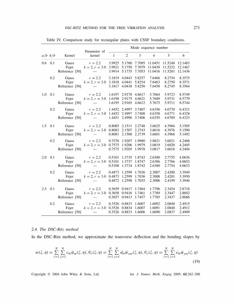
Table IV. Comparison study for rectangular plates with CSSF boundary conditions.


a/b h/b Kernel kernel 1 2 3 4 5 6

0.6 0.1 Gauss r = 2.2 3.9925 5.1760 7.7095 11.0451 11.5248 12.1483Fejer k = 2, r = 3.0 3.9921 5.1750 7.7079 11.0439 11.5232 12.1467

Reference [50] — 3.9914 5.1735 7.7053 11.0416 11.5201 12.1436

0.2 Gauss r = 2.2 3.1819 4.0443 5.8257 7.6466 8.2754 8.3575Fejer k = 2, r = 3.0 3.1818 4.0441 5.8254 7.6463 8.2750 8.3571

Reference [50] — 3.1817 4.0438 5.8250 7.6458 8.2745 8.3564

1.0 0.1 Gauss r = 2.2 1.6197 2.9170 4.6617 5.7684 5.9723 8.5749Fejer k = 2, r = 3.0 1.6198 2.9175 4.6621 5.7689 5.9731 8.5779

Reference [50] — 1.6195 2.9165 4.6612 5.7675 5.9711 8.5744

0.2 Gauss r = 2.2 1.4452 2.4997 3.7407 4.6356 4.6770 6.4321Fejer k = 2, r = 3.0 1.4452 2.4997 3.7408 4.6358 4.6771 6.4328

Reference [50] — 1.4451 2.4996 3.7406 4.6355 4.6769 6.4323

1.5 0.1 Gauss r = 2.2 0.8085 2.1511 2.2748 3.6625 4.3984 5.1505Fejer k = 2, r = 3.0 0.8083 2.1507 2.2743 3.6616 4.3976 5.1500

Reference [50] — 0.8081 2.1500 2.2739 3.6601 4.3968 5.1492

0.2 Gauss r = 2.2 0.7576 1.9207 1.9980 3.0821 3.6021 4.2406Fejer k = 2, r = 3.0 0.7575 1.9206 1.9979 3.0819 3.6020 4.2405

Reference [50] — 0.7575 1.9205 1.9978 3.0817 3.6018 4.2404

2.0 0.1 Gauss r = 2.2 0.5101 1.3735 1.8743 2.6380 2.7755 4.0636Fejer k = 2, r = 3.0 0.5101 1.3737 1.8747 2.6386 2.7766 4.0652

Reference [50] — 0.5100 1.3734 1.8742 2.6380 2.7754 4.0633

0.2 Gauss r = 2.2 0.4873 1.2599 1.7036 2.3007 2.4200 3.3949Fejer k = 2, r = 3.0 0.4873 1.2599 1.7036 2.3008 2.4201 3.3950

Reference [50] — 0.4872 1.2598 1.7035 2.3006 2.4199 3.3946

2.5 0.1 Gauss r = 2.2 0.3659 0.9417 1.7464 1.7796 2.3454 2.8718Fejer k = 2, r = 3.0 0.3658 0.9416 1.7461 1.7789 2.3447 2.8692

Reference [50] — 0.3657 0.9413 1.7457 1.7785 2.3437 2.8686

0.2 Gauss r = 2.2 0.3526 0.8833 1.6007 1.6092 2.0840 2.4915Fejer k = 2, r = 3.0 0.3526 0.8834 1.6007 1.6091 2.0840 2.4912

Reference [50] — 0.3526 0.8833 1.6006 1.6090 2.0837 2.4909

2.4. The DSC-Ritz method

In the DSC-Ritz method, we approximate the transverse deflection and the bending slopes by

w(�, �) =N∑

i=1

N∑j=1

cm m(�, �), �x(�, �) =N∑

i=1

N∑j=1

dm�xm(�, �), �y(�, �) =N∑

i=1

N∑j=1

em�ym(�, �)

(19)



Table V. Comparison study for rectangular plates with CFSF boundary conditions.


a/b h/b Kernel kernel 1 2 3 4 5 6

0.6 0.1 Gauss r = 2.2 3.8551 4.3259 5.9149 8.7782 10.9140 11.3617Fejer k = 2, r = 3.0 3.8546 4.3255 5.9122 8.7774 10.9129 11.3610

Reference [50] — 3.8539 4.3185 5.9067 8.7540 10.9102 11.3454

0.2 Gauss r = 2.2 3.0817 3.4128 4.5432 6.4929 7.5612 7.8452Fejer k = 2, r = 3.0 3.0816 3.4126 4.5424 6.4926 7.5614 7.8450

Reference [50] — 3.0815 3.4108 4.5416 6.4876 7.5603 7.8406

1.0 0.1 Gauss r = 2.2 1.4738 1.9536 3.6499 4.5031 5.0483 6.7909Fejer k = 2, r = 3.0 1.4737 1.9536 3.6483 4.5026 5.0479 6.7874

Reference [50] — 1.4735 1.9491 3.6452 4.5017 5.0395 6.7807

0.2 Gauss r = 2.2 1.3255 1.7030 3.0534 3.6265 4.0054 5.2086Fejer k = 2, r = 3.0 1.3254 1.7030 3.0530 3.6264 4.0052 5.2075

Reference [50] — 1.3254 1.7019 3.0526 3.6262 4.0031 5.2064

1.5 0.1 Gauss r = 2.2 0.6666 1.1014 2.1049 2.6693 2.8575 4.2273Fejer k = 2, r = 3.0 0.6665 1.1015 2.1047 2.6691 2.8565 4.2269

Reference [50] — 0.6664 1.0978 2.1044 2.6635 2.8547 4.2261

0.2 Gauss r = 2.2 0.6320 1.0008 1.8622 2.2975 2.4924 3.4779Fejer k = 2, r = 3.0 0.6320 1.0008 1.8622 2.2974 2.4922 3.4778

Reference [50] — 0.6320 0.9999 1.8621 2.2960 2.4920 3.4776

2.0 0.1 Gauss r = 2.2 0.3766 0.7610 1.2045 1.7474 2.4606 2.5667Fejer k = 2, r = 3.0 0.3766 0.7612 1.2043 1.7474 2.4604 2.5660

Reference [50] — 0.3765 0.7578 1.2041 1.7428 2.4599 2.5648

0.2 Gauss r = 2.2 0.3649 0.7025 1.1154 1.5614 2.1606 2.2777Fejer k = 2, r = 3.0 0.3648 0.7026 1.1153 1.5613 2.1601 2.2806

Reference [50] — 0.3648 0.7016 1.1152 1.5601 2.1600 2.2804

2.5 0.1 Gauss r = 2.2 0.2413 0.5817 0.7761 1.2859 1.5995 2.1852Fejer k = 2, r = 3.0 0.2412 0.5820 0.7760 1.2859 1.5992 2.1850

Reference [50] — 0.2412 0.5785 0.7759 1.2818 1.5991 2.1798

0.2 Gauss r = 2.2 0.2362 0.5409 0.7366 1.1714 1.4594 1.9300Fejer k = 2, r = 3.0 0.2362 0.5410 0.7365 1.1713 1.4593 1.9296

Reference [50] — 0.2362 0.5400 0.7365 1.1702 1.4592 1.9281

where N is the number of grid points in both x- and y-direction, cm, dm and em are theunknown coefficients, and the subscript m is determined by

m = (i − 1)N + j (20)

and

m = ��ij (�, �)Bw, �xm = ��ij (�, �)Bx, �ym = ��ij (�, �)By (21)



0 0.5 10

0.2

0.4

0.6

0.8

1

0 0.5 10

0.2

0.4

0.6

0.8

1

0 0.5 10

0.2

0.4

0.6

0.8

1

0 0.5 10

0.2

0.4

0.6

0.8

1

0 0.5 10

0.2

0.4

0.6

0.8

1

0 0.5 10

0.2

0.4

0.6

0.8

1

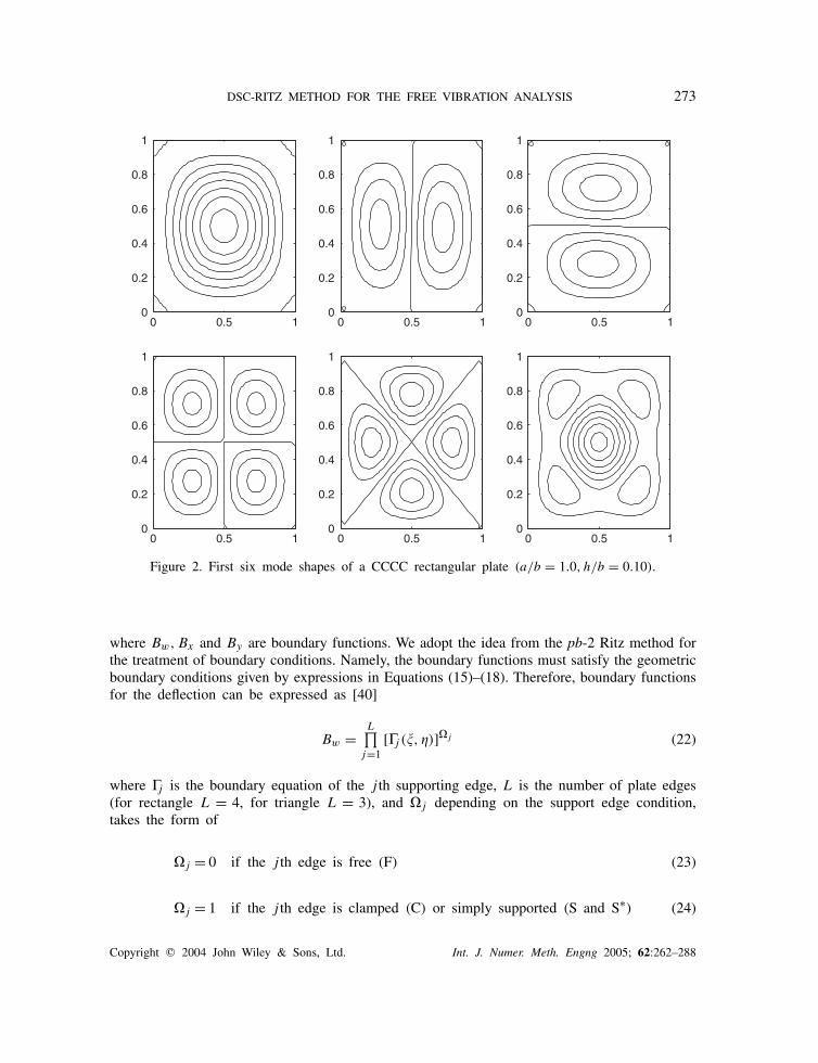
Figure 2. First six mode shapes of a CCCC rectangular plate (a/b = 1.0, h/b = 0.10).

where Bw, Bx and By are boundary functions. We adopt the idea from the pb-2 Ritz method forthe treatment of boundary conditions. Namely, the boundary functions must satisfy the geometricboundary conditions given by expressions in Equations (15)–(18). Therefore, boundary functionsfor the deflection can be expressed as [40]

Bw =L∏

j=1[�j (�, �)]�j (22)

where �j is the boundary equation of the j th supporting edge, L is the number of plate edges(for rectangle L = 4, for triangle L = 3), and �j depending on the support edge condition,takes the form of

�j = 0 if the j th edge is free (F) (23)

�j = 1 if the j th edge is clamped (C) or simply supported (S and S∗) (24)



0 0.5 10

0.2

0.4

0.6

0.8

1

0 0.5 10

0.2

0.4

0.6

0.8

1

0 0.5 10

0.2

0.4

0.6

0.8

1

0 0.5 10

0.2

0.4

0.6

0.8

1

0 0.5 10

0.2

0.4

0.6

0.8

1

0 0.5 10

0.2

0.4

0.6

0.8

1

Figure 3. First six mode shapes of an SSSS rectangular plate (a/b = 1.0, h/b = 0.10).

The boundary functions for the bending slopes can be expressed as

Bx =L∏

j=1[�j (�, �)]�j (25)

�j = 0 if the j th edge is free (F) or simply supported (S∗) or (S) in the y-direction

(26)

�j = 1 if the j th edge is clamped (C) or simply supported (S) in the x-direction(27)

and

By =L∏

j=1[�j (�, �)]�j (28)

�j = 0 if the j th edge is free (F) or simply supported (S∗) or (S) in the x-direction(29)



0 0.5 10

0.2

0.4

0.6

0.8

1

0 0.5 10

0.2

0.4

0.6

0.8

1

0 0.5 10

0.2

0.4

0.6

0.8

1

0 0.5 10

0.2

0.4

0.6

0.8

1

0 0.5 10

0.2

0.4

0.6

0.8

1

0 0.5 10

0.2

0.4

0.6

0.8

1

Figure 4. First six mode shapes of a CSSF rectangular plate (a/b = 1.0, h/b = 0.10).

�j = 1 if the j th edge is clamped (C) or simply supported (S) in the y-direction(30)

Note that ��ij (�, �) in Equation (21) is a DSC delta kernel. Up to an arbitrary constant whichis taken care by the minimization, the two-dimensional forms for the aforementioned two DSCkernels can be given by

��ij (x, y) = e−(x−xi)2/2�2

e−(y−yj )2/2�2(31)

for Gauss’ kernel, and

��ij (x, y) =sin2

(�

�(x − xi)

)sin2

(�

�(y − yj )

)sin2

(�

�(x − xi)/(2k + 1)

)sin2

(�

�(y − yj )/(2k + 1)

) , k = 1, 2, . . . (32)

for Fejer’s kernel. In all the above kernels, xi and yj are grid point co-ordinates along the x-and y-axis, respectively. The parameter � are chosen as � = r�, where � is the grid spacing,and r is an adjustable parameter determining the radius of influence, and is usually chosenbetween 1.0 and 3.0 in this work.



0 0.5 10

0.2

0.4

0.6

0.8

1

0 0.5 10

0.2

0.4

0.6

0.8

1

0 0.5 10

0.2

0.4

0.6

0.8

1

0 0.5 10

0.2

0.4

0.6

0.8

1

0 0.5 10

0.2

0.4

0.6

0.8

1

0 0.5 10

0.2

0.4

0.6

0.8

1

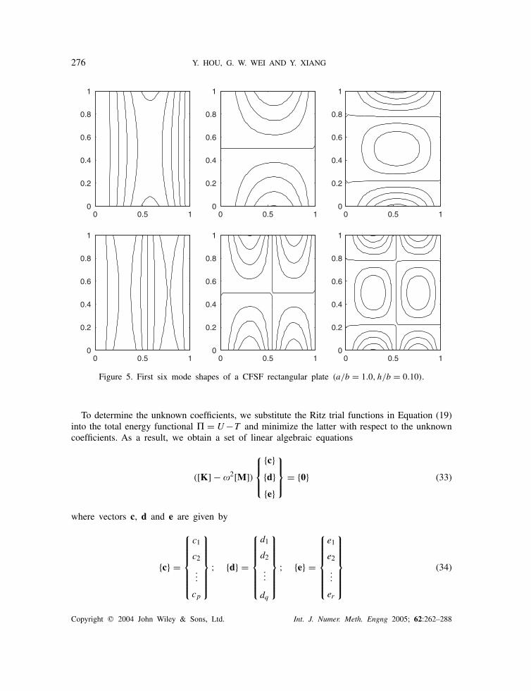
Figure 5. First six mode shapes of a CFSF rectangular plate (a/b = 1.0, h/b = 0.10).

To determine the unknown coefficients, we substitute the Ritz trial functions in Equation (19)into the total energy functional � = U −T and minimize the latter with respect to the unknowncoefficients. As a result, we obtain a set of linear algebraic equations

([K] − 2[M])

{c}{d}{e}

= {0} (33)

where vectors c, d and e are given by

{c} =

c1

c2

...

cp

; {d} =

d1

d2

...

dq

; {e} =

e1

e2

...

er

(34)



Table VI. Convergence study for triangular plates with CCC boundary conditions, h/b = 0.15.

Mode sequence numberNumber of

�◦ Kernel grid points 1 2 3 4 5 6

30◦ Gauss N = 7 6.4541 9.4010 12.1168 12.4831 15.9068 16.0461(r = 2.2) N = 8 6.4540 9.4005 12.1159 12.4624 15.6491 15.9005

N = 9 6.4538 9.4004 12.1155 12.4606 15.6164 15.8997N = 10 6.4537 9.4004 12.1152 12.4606 15.6133 15.8994

Fejer N = 6 6.4550 9.4189 12.1201 12.7464 15.9591 17.7321(r = 3.0) N = 7 6.4545 9.4046 12.1183 12.5210 15.9135 16.0755

N = 8 6.4544 9.4017 12.1171 12.4734 15.7607 15.9050N = 9 6.4543 9.4016 12.1167 12.4631 15.6429 15.9021

Reference [40] — 6.454 9.402 12.12 12.46 15.64 15.90

60◦ Gauss N = 7 10.2784 16.6672 16.6677 23.1279 23.9966 23.9975(r = 2.2) N = 8 10.2782 16.6671 16.6672 23.1275 23.9960 23.9966

N = 9 10.2782 16.6669 16.6671 23.1273 23.9959 23.9963N = 10 10.2781 16.6669 16.6670 23.1272 23.9958 23.9961

Fejer N = 6 10.2796 16.6704 16.6706 23.1634 24.0138 24.0473(r = 3.0) N = 7 10.2794 16.6697 16.6698 23.1322 24.0017 24.0034

N = 8 10.2794 16.6696 16.6697 23.1316 24.0004 24.0004N = 9 10.2794 16.6696 16.6696 23.1315 24.0003 24.0003

Reference [40] — 10.28 16.67 16.67 23.13 24.00 24.00

90◦ Gauss N = 7 15.9415 22.9157 26.5298 30.8848 33.9444 38.4088(r = 1.2) N = 8 15.9410 22.9155 26.5294 30.8834 33.8866 38.3859

N = 9 15.9411 22.9155 26.5288 30.8830 33.8857 38.3723N = 10 15.9409 22.9155 26.5289 30.8830 33.8854 38.3717

Fejer N = 6 15.9446 22.9264 26.5780 31.1306 34.1731 38.6439(r = 3.0) N = 7 15.9440 22.9208 26.5374 30.9030 34.0434 38.4578

N = 8 15.9438 22.9202 26.5348 30.8917 33.9053 38.4258N = 9 15.9438 22.9202 26.5342 30.8896 33.8958 38.3850

Reference [40] — 15.94 22.92 26.53 30.89 33.89 38.38

and they all have a common number of components

p = q = r = NN (35)

the matrix [K] has the structure of

[K] =

[Kcc] [Kcd ] [Kce][Kdd ] [Kde]

Symmetric [Kee]

(36)



Table VII. Impact study of parameter r on triangular plates with S*S*S* boundary con-ditions with apex angle � = 90◦, h/b = 0.15 and N = 10 for Gauss’ kernel and N = 9

for Fejer’s kernel.



Gauss r = 1.0 11.2942 19.2944 23.2819 28.1813 31.2322 36.2219r = 1.2 11.2787 19.2803 23.2763 28.1640 31.2255 36.2189r = 1.4 11.2754 19.2750 23.2750 28.1561 31.2218 36.2174r = 1.6 11.2748 19.2727 23.2745 28.1527 31.2197 36.2170r = 1.8 11.2746 19.2715 23.2744 28.1511 31.2184 36.2176r = 2.0 11.2744 19.2712 23.2743 28.1504 31.2187 36.2193r = 2.2 11.2757 19.2710 23.2743 28.1496 31.2201 36.2193r = 2.4 11.2753 19.2710 23.2690 28.1486 31.2194 36.2185r = 2.6 11.2888 19.2701 23.2744 28.1537 31.2796 36.2318r = 2.8 — — — — — —r = 3.0 — — — — — —

Fejer r = 1.0 — — — — — —(k = 2) r = 1.2 — — — — — —

r = 1.4 — — — — — —r = 1.6 12.0234 19.3896 23.4293 28.3548 31.2846 36.6767r = 1.8 11.4122 19.2952 23.3038 28.1863 31.2368 36.3158r = 2.0 11.2889 19.2777 23.2827 28.1621 31.2221 36.2448r = 2.2 11.2763 19.2738 23.2775 28.1567 31.2210 36.2483r = 2.4 11.2748 19.2725 23.2756 28.1535 31.2253 36.2591r = 2.6 11.2746 19.2718 23.2749 28.1520 31.2316 36.2694r = 2.8 11.2746 19.2715 23.2749 28.1520 31.2386 36.2781r = 3.0 11.2757 19.2740 23.2797 28.1580 31.2511 36.2927

Reference [50] — 11.28 19.27 23.28 28.16 31.24 36.28

Table VIII. Impact study of parameter k on triangular plates with S*S*S* boundaryconditions with a/b = 1.0, h/b = 0.1 and N = 9.



Fejer k = 1 — — — — — —(r = 3.0) k = 2 11.2757 19.2740 23.2797 28.1580 31.2511 36.2927

k = 3 11.2746 19.2716 23.2748 28.1522 31.2362 36.2750k = 4 11.2746 19.2718 23.2749 28.1527 31.2338 36.2713k = 5 11.2746 19.2719 23.2748 28.1523 31.2326 36.2698k = 6 11.2746 19.2720 23.2748 28.1523 31.2319 36.2689k = 7 11.2746 19.2720 23.2754 28.1524 31.2316 36.2683k = 8 11.2746 19.2720 23.2748 28.1524 31.2314 36.2680k = 9 11.2746 19.2720 23.2748 28.1524 31.2312 36.2677k = 10 11.2746 19.2720 23.2748 28.1524 31.2314 36.2680

Reference [50] — 11.28 19.27 23.28 28.16 31.24 36.28



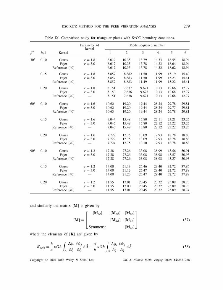
Table IX. Comparison study for triangular plates with S*CC boundary conditions.

Parameter of Mode sequence numberkernel

�◦ h/b Kernel 1 2 3 4 5 6

30◦ 0.10 Gauss r = 1.8 6.619 10.35 13.79 14.33 18.55 18.94Fejer r = 3.0 6.617 10.35 13.78 14.33 18.64 18.94

Reference [40] — 6.617 10.35 13.78 14.33 18.62 18.94

0.15 Gauss r = 1.8 5.857 8.882 11.50 11.99 15.19 15.40Fejer r = 3.0 5.857 8.883 11.50 11.99 15.23 15.41

Reference [40] — 5.857 8.883 11.49 11.99 15.22 15.41

0.20 Gauss r = 1.8 5.151 7.637 9.671 10.13 12.66 12.77Fejer r = 3.0 5.150 7.636 9.673 10.13 12.68 12.77

Reference [40] — 5.151 7.638 9.671 10.13 12.68 12.77

60◦ 0.10 Gauss r = 1.6 10.62 19.20 19.44 28.24 29.78 29.81Fejer r = 3.0 10.62 19.20 19.44 28.24 29.77 29.81

Reference [40] — 10.63 19.20 19.44 28.24 29.78 29.81

0.15 Gauss r = 1.6 9.044 15.48 15.80 22.11 23.21 23.26Fejer r = 3.0 9.045 15.48 15.80 22.12 23.22 23.26

Reference [40] — 9.045 15.48 15.80 22.12 23.22 23.26

0.20 Gauss r = 1.6 7.722 12.75 13.09 17.93 18.78 18.83Fejer r = 3.0 7.722 12.75 13.09 17.93 18.78 18.83

Reference [40] — 7.724 12.75 13.10 17.93 18.78 18.83

90◦ 0.10 Gauss r = 1.2 17.28 27.26 33.08 38.99 43.56 50.91Fejer r = 3.0 17.28 27.26 33.08 38.98 43.57 50.93

Reference [40] — 17.28 27.26 33.08 38.98 43.57 50.93

0.15 Gauss r = 1.2 14.00 21.13 25.46 29.40 32.72 37.86Fejer r = 3.0 14.00 21.13 25.47 29.40 32.72 37.88

Reference [40] — 14.00 21.23 25.47 29.40 32.72 37.88

0.20 Gauss r = 1.2 11.55 17.01 20.45 23.32 25.89 28.73Fejer r = 3.0 11.55 17.00 20.45 23.32 25.89 28.73

Reference [40] — 11.55 17.01 20.45 23.32 25.89 28.74

and similarly the matrix [M] is given by

[M] =

[Mcc] [Mcd ] [Mce][Mdd ] [Mde]

Symmetric [Mee]

(37)

where the elements of [K] are given by

Kccij = b

aGh

∫A

� i

��

� j

��dA + a

bGh

∫A

� i

��

� j

��dA (38)



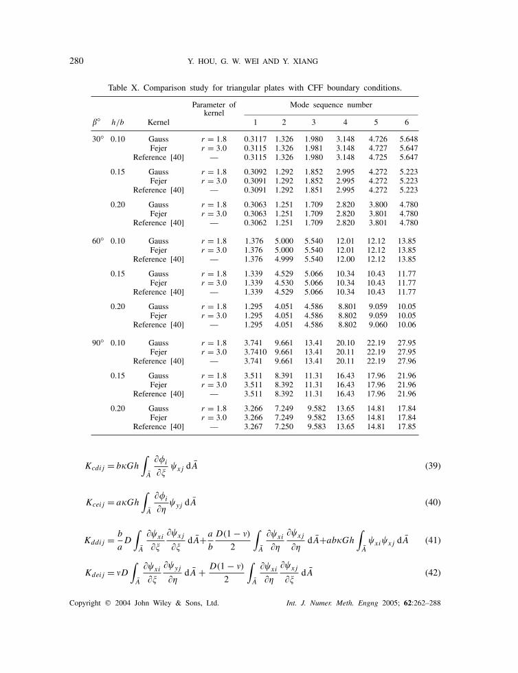
Table X. Comparison study for triangular plates with CFF boundary conditions.

Parameter of Mode sequence numberkernel

�◦ h/b Kernel 1 2 3 4 5 6

30◦ 0.10 Gauss r = 1.8 0.3117 1.326 1.980 3.148 4.726 5.648Fejer r = 3.0 0.3115 1.326 1.981 3.148 4.727 5.647

Reference [40] — 0.3115 1.326 1.980 3.148 4.725 5.647

0.15 Gauss r = 1.8 0.3092 1.292 1.852 2.995 4.272 5.223Fejer r = 3.0 0.3091 1.292 1.852 2.995 4.272 5.223

Reference [40] — 0.3091 1.292 1.851 2.995 4.272 5.223

0.20 Gauss r = 1.8 0.3063 1.251 1.709 2.820 3.800 4.780Fejer r = 3.0 0.3063 1.251 1.709 2.820 3.801 4.780

Reference [40] — 0.3062 1.251 1.709 2.820 3.801 4.780

60◦ 0.10 Gauss r = 1.8 1.376 5.000 5.540 12.01 12.12 13.85Fejer r = 3.0 1.376 5.000 5.540 12.01 12.12 13.85

Reference [40] — 1.376 4.999 5.540 12.00 12.12 13.85

0.15 Gauss r = 1.8 1.339 4.529 5.066 10.34 10.43 11.77Fejer r = 3.0 1.339 4.530 5.066 10.34 10.43 11.77

Reference [40] — 1.339 4.529 5.066 10.34 10.43 11.77

0.20 Gauss r = 1.8 1.295 4.051 4.586 8.801 9.059 10.05Fejer r = 3.0 1.295 4.051 4.586 8.802 9.059 10.05

Reference [40] — 1.295 4.051 4.586 8.802 9.060 10.06

90◦ 0.10 Gauss r = 1.8 3.741 9.661 13.41 20.10 22.19 27.95Fejer r = 3.0 3.7410 9.661 13.41 20.11 22.19 27.95

Reference [40] — 3.741 9.661 13.41 20.11 22.19 27.96

0.15 Gauss r = 1.8 3.511 8.391 11.31 16.43 17.96 21.96Fejer r = 3.0 3.511 8.392 11.31 16.43 17.96 21.96

Reference [40] — 3.511 8.392 11.31 16.43 17.96 21.96

0.20 Gauss r = 1.8 3.266 7.249 9.582 13.65 14.81 17.84Fejer r = 3.0 3.266 7.249 9.582 13.65 14.81 17.84

Reference [40] — 3.267 7.250 9.583 13.65 14.81 17.85

Kcdij = bGh

∫A

� i

��xj dA (39)

Kceij = aGh

∫A

� i

��yj dA (40)

Kddij = b

aD

∫A

��xi

��

��xj

��dA+a

b

D(1 − �)

2

∫A

��xi

��

��xj

��dA+abGh

∫A

�xi�xj dA (41)

Kdeij = �D∫

A

��xi

��

��yj

��dA + D(1 − �)

2

∫A

��xi

��

��xj

��dA (42)



a

β

b/2

b/2

Figure 6. Geometry of a triangular Mindlin plate.

Figure 7. First six mode shapes of a CCC right angled isoscelestriangular plate with base length b (h/b = 0.15).

Keeij = a

bD

∫A

��yi

��

��yj

��dA + b

a

D(1 − �)

2

∫A

��yi

��

��yj

��dA + abGh

∫A

�yi�yj dA (43)

where

i = 1, 2, . . . , p; j = 1, 2, . . . , p



Figure 8. First six mode shapes of an S*S*S* right angled isoscelestriangular plate with base length b (h/b = 0.15).

Figure 9. First six mode shapes of an S*CC right angled isoscelestriangular plate with base length b (h/b = 0.15).

for all of the above-mentioned elements. Finally, the entries of [M] are given by

Mccij = ab�h

∫A

i j dA (44)



Figure 10. First six mode shapes of a CFF right angled isoscelestriangular plate with base length b (h/b = 0.15).

Mcdij = 0 (45)

Mceij = 0 (46)

Mddij = 1

12ab�h3

∫A

�xi�xj dA (47)

Mdeij = 0 (48)

Meeij = 1

12ab�h3

∫A

�yi�yj dA (49)

where

i = 1, 2, . . . , p; j = 1, 2, . . . , p

and for simplicity, we choose p = N × N in this work.For vibration analysis, our objective is to obtain the frequency parameter, , which can

be accomplished by solving the generalized eigenvalue problem defined by Equation (33). Weresort to a standard eigenvalue solver for the solution of Equation (33).

3. NUMERICAL RESULTS AND DISCUSSION

In this section, we explore the usefulness and test the accuracy of the DSC-Ritz method.Consideration is given to the first six frequency parameters for thick rectangular and isosceles



triangular plates with different combinations of simply supported, clamped and free edges. Notethat a simply supported edge for the rectangular plate is considered to be the first type (S) andfor the triangular plates is treated as the second type (S*) in the paper. Numerical integrations arecarried out by using Gaussian quadratures with appropriate number of polynomials (about 50).

3.1. Rectangular plates

For brevity and convenience, a four-letter symbol is used to denote the support conditions ofa rectangular Mindlin plate. For example, an SCFS plate has a simply supported left edge,a clamped bottom edge, a free right edge and a simply supported top edge, respectively. Forthe purpose of comparison study, numerical calculations have been performed for rectangularMindlin plates of four different combinations of edge support conditions, namely CCCC, SSSS,CSSF, and CFSF plates. The vibration frequencies of a rectangular Mindlin plate are expressedin terms of a non-dimensional frequency parameter � = (b2/�2)

√�h/D , where b is the

width of the plate.The Poisson’s ratio � = 0.3 and the shear correction factor = 5

6 have been used in thecalculation.

Convergence studies have been carried out for the CCCC plate. By varying the number ofuniform DSC grid points N both in x and y directions, the convergence patterns of the firstsix frequency parameters have been investigated. The results are summarized in Table I for thecases of thick rectangular plates with plate thickness ratios h/b = 0.1 and 0.2, plate aspectratios a/b = 1.0 and 2.0, and r = 1.8 for the Gauss kernel and r = 3.0 and k = 2 for theFejer kernel, respectively. The pb-2 Ritz results [50] have also been given in Table I for acomparison.

Table I shows that the frequency parameters decrease as the number of DSC grid pointsvaries from 2 to 7. For most cases, the frequency parameters for the CCCC plate have achievedgood convergence even with the number of DSC grid points N = 6. When the number ofgrid points N increase from 6 to 9, the frequency parameters oscillate slightly around thoseof the reference pb-2 Ritz. It is evident from the convergence studies that, in general, whenthe number of DSC grid points is set to be N = 9 for both Gauss’ kernel and Fejer’s kernel,the DSC-Ritz method will produce accurate and reliable frequency parameters for rectangularMindlin plates. All subsequent calculations for rectangular Mindlin plates are based on N = 9.

Tables II and III show the impact of kernel parameters r and k on the frequency parametersof SSSS rectangular plates. It is evident that the DSC-Ritz method is robust against parametervariation. The selection of r = 1.8 for the Gauss kernel and r = 3.0 and k = 2 for the Fejerkernel is appropriate for the present calculation.

These convergence and impact studies have established our confidence on the robustnessand reliability of the DSC-Ritz method. To further explore the application of the methodto rectangular plates with different combinations of edge support conditions, the first six fre-quency parameters for CSSF and CFSF rectangular Mindlin plates are computed with the Gausskernel and the Fejer kernel and presented in Tables IV and V. The plate thickness is set tobe h/b = 0.1 and 0.2 and the plate aspect ratio is taken as a/b = 0.6, 1.0, 1.5, 2.0 and 2.5,respectively. The pb-2 Ritz results from Reference [50] are also presented in Tables IV and V.Excellent agreement is observed between the DSC-Ritz and pb-2 Ritz frequency parameters forall considered cases. Such agreement confirms the validity of the proposed DSC-Ritz methodfor vibration analysis of rectangular Mindlin plates.



Figures 2–5 present the mode contour shapes for the first six modes of the CCCC, SSSS,CSSF, and CFSF square plates with plate thickness h/b = 0.10. We observe that the modeshapes for square Mindlin plates of various edge support conditions are correctly predicted bythe DSC-Ritz method.

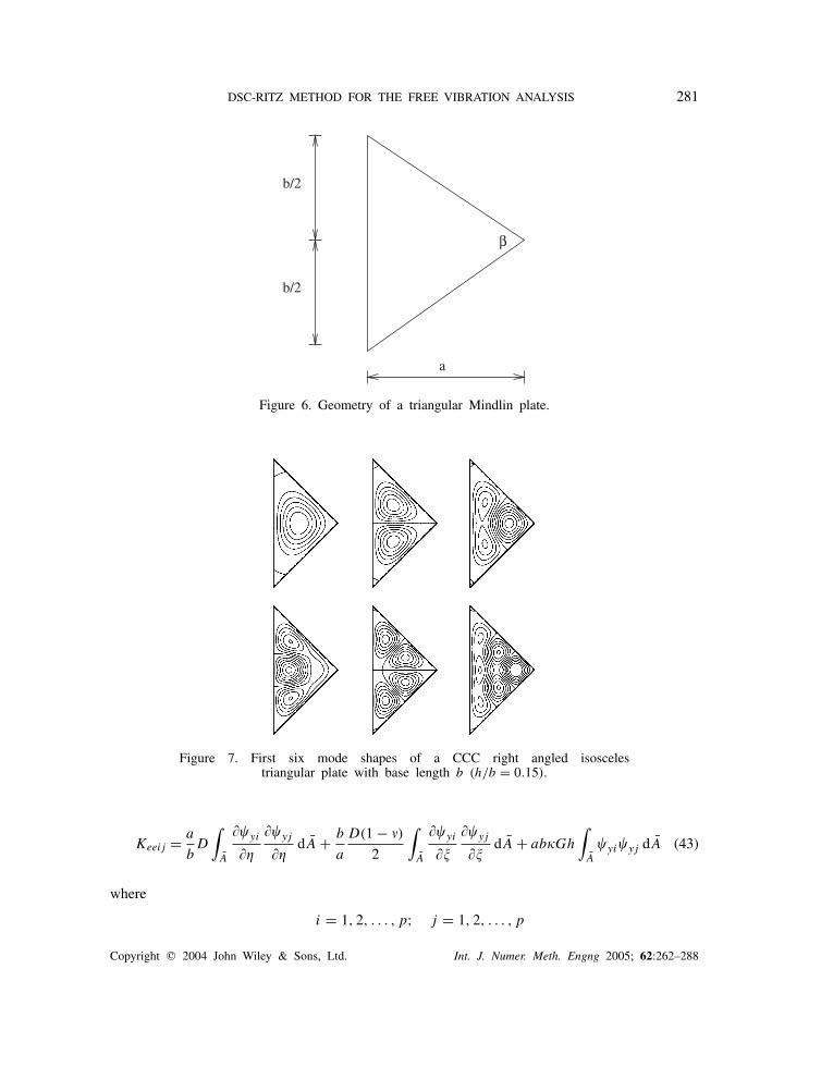
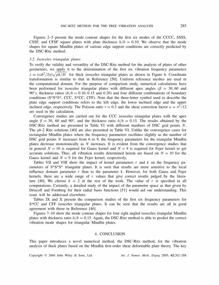
3.2. Isosceles triangular platesTo verify the validity and versatility of the DSC-Ritz method for the analysis of plates of othergeometries, we apply it to the determination of the first six vibration frequency parameters� = (b2/2�)

√�h/D for thick isosceles triangular plates as shown in Figure 6. Coordinate

transformation is similar to that in Reference [50]. Uniform reference meshes are used inthe computational domain. For the purpose of comparison study, numerical calculations havebeen performed for isosceles triangular plates with different apex angles (� = 30, 60 and90◦), thickness ratios (h/b = 0.10, 0.15 and 0.20) and four different combinations of boundaryconditions (S*S*S*, CCC, S*CC, CFF). Note that the three-letter symbol used to describe theplate edge support conditions refers to the left edge, the lower inclined edge and the upperinclined edge, respectively. The Poisson ratio � = 0.3 and the shear correction factor = �2/12are used in the calculation.

Convergence studies are carried out for the CCC isosceles triangular plates with the apexangle � = 30, 60 and 90◦, and the thickness ratio h/b = 0.15. The results obtained by theDSC-Ritz method are presented in Table VI with different numbers of DSC grid points N .The pb-2 Ritz solutions [40] are also presented in Table VI. Unlike the convergence cases forrectangular Mindlin plates where the frequency parameters oscillates slightly as the number ofDSC grid points N increases from 6 to 9, the frequency parameters for the triangular Mindlinplates decrease monotonically as N increases. It is evident from the convergence studies thatin general N = 10 is required for Gauss kernel and N = 9 is required for Fejer kernel to getaccurate solutions. Thus, all vibration results determined herein are based on N = 10 for theGauss kernel and N = 9 for the Fejer kernel, respectively.

Tables VII and VIII show the impact of kernel parameters r and k on the frequency pa-rameters of S*S*S* triangular plates. It is seen that results are more sensitive to the localinfluence domain parameter r than to the parameter k. However, for both Gauss and Fejerkernels, there are a wide range of r values that give correct results judged by the litera-ture [40]. We choose k = 2 in the rest of the work. The value of r is specified in allcomputations. Certainly, a detailed study of the impact of the parameter space as that given byDriscoll and Fornberg for their radial basis functions [51] would aid our understanding. Thisissue will be addressed elsewhere.

Tables IX and X present the comparison studies of the first six frequency parameters forS*CC and CFF isosceles triangular plates. It can be seen that the results are all in goodagreement with those in Reference [40].

Figures 7–10 show the mode contour shapes for four right angled isosceles triangular Mindlinplates with thickness ratio h/b = 0.15. Again, the DSC-Ritz method is able to predict the correctvibration mode shapes for triangular Mindlin plates.

4. CONCLUSION

This paper introduces a novel numerical method, the DSC-Ritz method, for the vibrationanalysis of thick plates based on the Mindlin first-order shear deformable plate theory. The key



idea is to take the advantage of DSC local delta sequence kernels and the pb-2 Ritz boundaryfunctions. Two DSC delta sequence kernels of positive type are employed to construct new basisfunctions. The Ritz variational principle is utilized to determine unknown expansion coefficientsand to arrive at a set of generalized eigenvalue equations. The solution of the generalizedeigenvalue equations results in the desirable frequency parameters and modal shapes. Numericalexperiments are conducted for rectangular plates and triangular plates with various combinationsof simply supported, clamped and free edge conditions. The reliability and robustness of theproposed method are carefully validated by extensive convergence tests and by a comparisonwith those in the literature. Numerical results indicate that the proposed DSC-Ritz method isa simple approach for the vibration analysis of Mindlin plates.

Comparing to our previous DSC algorithm, which makes use of delta sequence kernelsof Dirichlet type and the collocation formulation for differential equations, the present DSC-Ritz method employs delta sequence kernels of positive type and is relied on Ritz energyminimization principle (essentially the Galerkin formulation). Obviously, the philosophy ofdiscrete approximations to the singular delta distribution, i.e. the universal reproducing kernel,underpins both DSC methods. We believe that these DSC methods are promising new approachesfor structural analysis in general.

REFERENCES

1. Chladni EFF. Entdeckungen uber die Theorie des Klanges. Weidmanns Erben & Reich: Leipzig, 1787.2. Kirchhoff G. Uber das gleichgwich und die bewegung einer elastischen scheibe. Journal of Angew Mathematics

1850; 40:51–88.3. Reissner E. The effect of transverse shears deformation on the bending of elastic plate. Journal of Applied

Mechanics (ASME) 1945; 12:69–76.4. Mindlin RD. Influence of rotary inertia and shear in flexural motion of isotropic, elastic plates. Journal of

Applied Mechanics (ASME) 1951; 18:1031–1036.5. Leissa AW. Vibration of Plates (NASA SP 160). U.S. Government Printing Office: Washington DC, 1969.6. Gorman DJ. Highly accurate analytical solution for free vibration analysis of simply supported right triangular

plates. Journal of Sound and Vibration 1983; 89:107–118.7. Warburton GB. The vibration of rectangular plates. Proceedings of the Institute of Mechanical Engineering

1954; 168:371–384.8. Young D. Vibration of rectangular plates by the Ritz method. Journal of Applied Mechanics (ASME) 1950;

17:448–453.9. Durvasula S. Nature frequencies and modes of skew membranes. Journal of Acoustical Society of America

1968; 44:1636–1646.10. Leissa AW. The free vibration of rectangular plates. Journal of Sound Vibration 1973; 31:257–293.11. Mizusawa T. Natural frequencies of rectangular plates with free edges. Journal of Sound and Vibration 1986;

105:451–459.12. Martin AF, Leissa AW. Application of the Ritz method to plane elasticity problems for composite sheets with

variable fiber spacing. International Journal for Numerical Methods in Engineering 1989; 28:1813–1825.13. Wang S. A unified Timoshenko beam B-spline Rayleigh–Ritz method for vibration and buckling analysis

of thick and thin beams and plates. International Journal for Numerical Methods in Engineering 1997;40:473–491.

14. Smith ST, Bradford MA, Oehlers D. Numerical convergence of simple and orthogonal polynomials forthe unilateral plate buckling problem using the Rayleigh–Ritz method. International Journal for NumericalMethods in Engineering 1999; 44:1685–1707.

15. Narita Y. Application of a series-type method to vibration of orthotropic rectangular plates with mixedboundary conditions. Journal of Sound and Vibration 1981; 77:345–355.

16. Laura PAA, Gutierrez RH. Analysis of vibrating rectangular plates with nonuniform boundary conditions byusing the differential quadrature method. Journal of Sound and Vibration 1994; 173:702–706.



17. Shu C, Wang CM. Implementation of clamped and simply supported boundary conditions in the GDQ freevibration analysis of beams and plates. International Journal of Solids and Structures 1997; 34:819–835.

18. Shu C, Wang CM. Treatment of mixed and nonuniform boundary conditions in GDQ vibration analysis ofrectangular plates. Engineering Structures 1999; 21:125–134.

19. Cheung YK, Cheung MS. Flexural vibration of rectangular and other polygonal plates. Proceedings ofASCE Journal of the Engineering Mechanics Division 1971; 97:391–411.

20. Fan SC, Cheung YK. Flexural free vibrations of rectangular plates with complex support conditions. Journalof Sound and Vibration 1984; 93:81–94.

21. Zienkiewicz OC. Achievements and some unsolved problems of the finite element method. InternationalJournal for Numerical Methods in Engineering 2000; 47:9–28.

22. Wei GW. Discrete singular convolution for the solution of the Fokker–Planck equations. Journal of ChemicalPhysics 1999; 110:8930–8942.

23. Wei GW. A unified approach for the solution of the Fokker–Planck equations. Journal of Physics A:Mathematics and General 2000; 33:4935–4953.

24. Wei GW, Zhao YB, Xiang Y. Discrete singular convolution and its application to the analysis of plateswith internal supports. I. Theory and algorithm. International Journal for Numerical Methods in Engineering2002; 55:913–946.

25. Zhou YC, Patnaik BSV, Wan DC, Wei GW. DSC solution for flows in a staggered double lid driven cavity.International Journal for Numerical Methods in Engineering 2003; 57:211–234.

26. Bao G, Wei GW, Zhao S. Numerical solution of the Helmholtz equation with high wave numbers. InternationalJournal for Numerical Methods in Engineering 2004; 59:389–408.

27. Wei GW. Vibration analysis by discrete singular convolution. Journal of Sound and Vibration 2001; 244:535–553.

28. Wei GW. Discrete singular convolution for beam analysis. Engineering Structure 2001; 23:1045–1053.29. Wei GW. A new algorithm for solving some mechanical problems. Computer Methods for Applied Mechanics

and Engineering 2001; 190:2017–2030.30. Wei GW, Zhao YB, Xiang Y. The determination of natural frequencies of rectangular plates with mixed

boundary conditions by discrete singular convolution. International Journal of Mechanical Sciences 2001;43:1731–1746.

31. Wei GW, Zhao YB, Xiang Y. A novel approach for the prediction and control of high frequency vibration.Journal of Sound and Vibration 2002; 257:207–246.

32. Xiang Y, Zhao YB, Wei GW. Discrete singular convolution and its application to the analysis of plates withinternal supports. II. Complex supports. International Journal for Numerical Methods in Engineering 2002;55:947–971.

33. Zhao YB, Wei GW. DSC analysis rectangular plates with nonuniform boundary conditions. Journal of Soundand Vibration 2002; 255:203–225.

34. Zhao YB, Wei GW, Xiang Y. Discrete singular convolution for the prediction of high frequency vibrationof plates. International Journal of Solids and Structures 2002; 39:65–68.

35. Zhao YB, Wei GW, Xiang Y. Plate vibration under irregular internal supports. International Journal of Solidsand Structures 2002; 39:1361–1383.

36. Liew KM, Wang CM, Xiang Y, Kitipornchai S. Vibration of Mindlin Plate, Programming the p-versionMethod. Elsevier: Amsterdam, 1998.

37. Kitipornchai S, Xiang Y, Wang CM, Liew KM. Buckling of thick skew plates. International Journal forNumerical Methods in Engineering 1993; 36:1299–1310.

38. Dickinson SM, Li EKH. On the use of simply supported plate functions in the Rayleigh–Ritz methodapplied to the flexural vibration of triangular plates. Journal of Sound and Vibration 1982; 80:292–297.

39. Nanni J. Das Eulersche Knickproblem unter beruksichtigung der querkrafte. Zeitschrift fur AngewandteMathematik and Physik 1971; 22:156–185.

40. Kitipornchai S, Xiang Y, Wang CM, Liew KM. Free vibration of isosceles triangular Mindlin plates.International Journal of Mechanical Sciences 1993; 35:89–102.

41. Liew KM, Xiang Y, Wang CM, Kitipornchai S. Flexural vibration of shear deformable circular and annularplates on ring supports. Computer Methods in Applied Mechanics and Engineering 1993; 110:301–315.

42. Xiang Y, Wang CM, Kitipornchai S. Buckling of skew Mindlin plates subjected to in-plane shear loadings.International Journal of Mechanical Sciences 1995; 37:1089–1101.

43. Xiang Y, Wang CM, Kitipornchai S. FORTRAN subroutines for mathematical operations on polynomialfunctions. Computers and Structures 1995; 56:541–551.



44. Wei GW, Xiang Y. DSC-Ritz method for the analysis of beams and plates, 2003, to be published.45. Lucy LB. A numerical approach to the testing of the fission hypothesis. The Astrophysical Journal 1977;

82:1013–1024.46. Monaghan JJ. An introduction to SPH. Computer Physics Communication 1988; 48:89–96.47. Liu WK, Jun S, Li S, Adee J, Belytschko T. Reproducing kernel particle method for structural dynamics.

International Journal for Numerical Methods in Engineering 1995; 38:1655–1679.48. Liew KW, Zhao X, Ng TN. The element-free kp-Ritz method for vibration of laminated rotating cylindrical

panels. International Journal of Structural Stability and Dynamics 2002; 2:523–558.49. Zhao X, Liew KW, Ng TN. Vibration analysis of laminated composite cylindrical panels via a meshfree

approach. International Journal of Solids and Structures 2003; 40:161–180.50. Liew KM, Xiang Y, Kitipornchai S. Transverse vibration of thick rectangular plates–I: comprehensive sets

of boundary conditions. Computers and Structures 1993; 49:1–29.51. Driscoll TA, Fornberg B. Interpolation in the limit of increasingly flat radial basis functions. Computers and

Mathematics with Applications 2002; 43:413–422.


dsc-ritz method for the free vibration analysis of mindlin plates

Documents

discrete singular convolution

discrete singular convolution

michigan state university

angled isoscelestriangular plate

nonuniform boundary conditions

mode sequence numberkernel

universal reproducing kernel

ssss boundary conditionswith