dsa channel sounding dissertation
TRANSCRIPT
Wideband Channel SoundingTechniques for Dynamic Spectrum
Access Networks
Qi Chen
Submitted to the Graduate Degree Program in ElectricalEngineering & Computer Science and the Graduate Faculty
of the University of Kansas in partial fulfillment of therequirements for the degree of Doctor of Philosophy
Dissertation Committee:
Dr. Gary J. Minden: Chairperson
Dr. James A. Roberts
Dr. Alexander M. Wyglinski
Dr. Erik S. Perrins
Dr. Tyrone E. Duncan
Date Defended
The Dissertation Committee for Qi Chen certifies
that this is the approved version of the following dissertation:
Wideband Channel Sounding Techniques for Dynamic Spectrum
Access Networks
Committee:
Dr. Gary J. Minden,
Professor, EECS
Dr. James A. Roberts,
Professor, EECS
Dr. Alexander M. Wyglinski,
Assistant Professor, ECE, WPI
Dr. Erik S. Perrins,
Assistant Professor, EECS
Dr. Tyrone E. Duncan,
Professor, Mathematics
Date Approved
i

Abstract
In recent years, cognitive radio has drawn extensive research attention due
to its ability to improve the efficiency of spectrum usage by allowing dynamic
spectrum resource sharing between primary and secondary users. The concept of
cognitive radio was first presented by Joseph Mitola III and Gerald Q. Maguire,
Jr., in which either network or wireless node itself changes particular transmission
and reception parameters to execute its tasks efficiently without interfering with
the primary users [1]. Such a transceiving mechanism and network environment
is called the dynamic spectrum access (DSA) network. The Federal Communi-
cations Commission (FCC) allows any type of transmission in unlicensed bands
at any time as long as their transmit power level obeys specific FCC regulations.
Performing channel sounding as a secondary user in such an environment becomes
a challenge due to the rapidly changing network environment and also the limited
transmission power. Moreover, to obtain the long term behavior of the channel
in the DSA network is impractical with conventional channel sounders due to fre-
quent changes in frequency, transmission bandwidth, and power. Conventional
channel sounding techniques need to be adapted accordingly to be operated in
the DSA networks.
In this dissertation, two novel channel sounding system frameworks are pro-
posed. The Multicarrier Direct Sequence Swept Time-Delay Cross Correlation
(MC-DS-STDCC) channel sounding technique is designed for the DSA networks
aiming to perform channel sounding across a large bandwidth with minimal in-
terference. It is based on the STDCC channel sounder and Multicarrier Direct
Sequence Code Division Multiple Access (MC-DS-CDMA) technique. The STDCC
technique, defined by Parsons [2], was first employed by Cox in the measurement of
910 MHz band [3–6]. The MC-DS-CDMA technique enables the channel sounder
to be operated at different center frequencies with low transmit power. Hence,
interference awareness and frequency agility are achieved. The OFDM-based chan-
nel sounder is an alternative to the MC-DS-STDCC technique. It utilizes user data
as the sounding signal such that the interference is minimized during the course
of transmission. Furthermore, the OFDM-based channel sounder requires lower
sampling rate than the MC-DS-STDCC system since no spreading is necessary.
ii

To my parents and my lovely wife Jin Zhu
iii
Acknowledgments
First, I would like to express my deepest gratitude to my advisor Professor
Gary J. Minden for his excellent guidance and continual support during the course
of my degree. Second, I would like thank Dr. Alexander M. Wyglinski (former
assistant research professor at the University of Kansas) at Worcester Polytech-
nic Institute for being such a good friend, and for providing generous help and
guidance throughout my research. Working with them was a wonderful experi-
ence. I am very grateful for their time and patience dedicated to my research and
dissertation.
The financial support provided by the National Science Foundation under the
project “National Radio Testbed” as well as the EECS department are duly ac-
knowledged. I would like to thank Professor James A. Roberts for providing me
the opportunity at the University of Kansas for pursuing a Ph.D. degree. I would
also like to thank Professor John Gauch for accepting and processing my late
application.
I would like to thank Professor Erik S. Perrins and Professor Tyrone Duncan
for agreeing to be on my committee. During my time at the University of Kansas,
I met numerous students, faculty and staff in the Information and Telecommunica-
tion Technology Center (ITTC), the Electrical Engineering and Computer Science
department, and the University of Kansas in general, who have made my Ph.D.
experience all the more rewarding, and to them I owe my thanks. In particular,
I would like to thank Tim Newman, Biao Fu, Rakesh Rajbanshi, Dinesh Datla,
Mike Hulet, Annie Francis, and Paula Conlin. I would also like to thank Dan
Depardo and Leon Searl for sharing their professional knowledge, for helping me
solve problems during my research and other staff at ITTC who have directly or
indirectly helped me complete my studies successfully.
As always, I am deeply indebted to my parents. Without their generous sup-
port, I would not have completed all my achievements. Finally, I would like to
thank my lovely wife Jin for her love, understanding, support, and unwavering
belief in me.
iv

Contents
Acceptance Page i
Abstract ii
Acknowledgments iv
1 Introduction 1
1.1 Research Motivation . . . . . . . . . . . . . . . . . . . . . . . . . 1
1.2 Implementation: A Whole New Story . . . . . . . . . . . . . . . . 4
1.3 Current State-of-the-Art . . . . . . . . . . . . . . . . . . . . . . . 5
1.4 Dissertation Contributions . . . . . . . . . . . . . . . . . . . . . . 6
1.5 Dissertation Organization . . . . . . . . . . . . . . . . . . . . . . 8
2 Radio Propagation Channel 11
2.1 Fundamentals of Mobile Radio Channel . . . . . . . . . . . . . . . 11
2.2 Multipath Fading Channel . . . . . . . . . . . . . . . . . . . . . . 12
2.3 Time and Frequency Domain Characteristics . . . . . . . . . . . . 13
2.3.1 Delay Spread, Power Delay Profile and rms Delay Spread . 13
2.4 Channel Coherence . . . . . . . . . . . . . . . . . . . . . . . . . . 18
2.4.1 Coherence versus Selectivity . . . . . . . . . . . . . . . . . 18
2.4.2 Temporal Coherence . . . . . . . . . . . . . . . . . . . . . 19
2.4.3 Frequency Coherence . . . . . . . . . . . . . . . . . . . . . 20
2.5 Radio Channel Characteristics of the Dynamic Spectrum Access
Network Environment . . . . . . . . . . . . . . . . . . . . . . . . 22
2.6 Chapter Summary . . . . . . . . . . . . . . . . . . . . . . . . . . 25
v

3 Channel Sounding Techniques 27
3.1 Radio Channel Sounding . . . . . . . . . . . . . . . . . . . . . . . 28
3.2 Periodic Pulse Channel Sounding . . . . . . . . . . . . . . . . . . 29
3.3 Frequency Domain Channel Sounder: Chirp Sounder . . . . . . . 30
3.4 Pulse Compression . . . . . . . . . . . . . . . . . . . . . . . . . . 31
3.4.1 Convolution Matched Filter . . . . . . . . . . . . . . . . . 33
3.5 The STDCC Technique . . . . . . . . . . . . . . . . . . . . . . . . 33
3.5.1 Overview . . . . . . . . . . . . . . . . . . . . . . . . . . . 34
3.5.2 System Parameters . . . . . . . . . . . . . . . . . . . . . . 36
3.5.2.1 Multipath Resolution . . . . . . . . . . . . . . . . 37
3.5.2.2 Dynamic Range . . . . . . . . . . . . . . . . . . . 37
3.5.2.3 Time Scaling Factor . . . . . . . . . . . . . . . . 39
3.5.2.4 Doppler-shift Resolution . . . . . . . . . . . . . . 39
3.6 Frequency Domain Characterization . . . . . . . . . . . . . . . . . 41
3.7 Chapter Summary . . . . . . . . . . . . . . . . . . . . . . . . . . 42
4 Multicarrier Direct Sequence Sounder 43
4.1 MC-DS-CDMA System . . . . . . . . . . . . . . . . . . . . . . . . 44
4.2 Combined STDCC MC-DS-CDMA Implementation . . . . . . . . 46
4.2.1 Channel Impulse Response Estimation . . . . . . . . . . . 51
4.2.2 Dynamic Range Performance . . . . . . . . . . . . . . . . 53
4.2.3 Assessing the Impact of the Proposed Channel Sounding
Technique . . . . . . . . . . . . . . . . . . . . . . . . . . . 60
4.3 Simulation Results and Analysis . . . . . . . . . . . . . . . . . . . 61
4.3.1 Simulation Setup . . . . . . . . . . . . . . . . . . . . . . . 61
4.3.2 STDCC Simulation Results . . . . . . . . . . . . . . . . . 62
4.3.3 MC-DS-STDCC Simulation Results . . . . . . . . . . . . . 71
4.3.4 Mean Squared Error of the CIR Estimation . . . . . . . . 73
4.4 Chapter Summary . . . . . . . . . . . . . . . . . . . . . . . . . . 79
5 OFDM-Based Channel Sounder 80
5.1 Ultra Wideband Channel Sounder . . . . . . . . . . . . . . . . . . 80
5.2 OFDM Systems Overview . . . . . . . . . . . . . . . . . . . . . . 81
5.3 OFDM-Based Channel Sounder for Cognitive Radios . . . . . . . 84
vi

5.3.1 System Parameters . . . . . . . . . . . . . . . . . . . . . . 87
5.4 Sounding Signal and Performance . . . . . . . . . . . . . . . . . . 89
5.4.1 Guaranteed Spectrum Availability . . . . . . . . . . . . . . 89
5.4.2 Non-Contiguous Band . . . . . . . . . . . . . . . . . . . . 93
5.4.3 Sounding Signal Performance Analysis and Simulation Results 94
5.5 Chapter Summary . . . . . . . . . . . . . . . . . . . . . . . . . . 104
6 Implementation of STDCC Channel Sounder 105
6.1 USRP Hardware Prototyping Platform . . . . . . . . . . . . . . . 105
6.1.1 Signal Processing . . . . . . . . . . . . . . . . . . . . . . . 109
6.2 Implementations of STDCC . . . . . . . . . . . . . . . . . . . . . 110
6.2.1 In Building Setup and Measurements . . . . . . . . . . . . 113
6.2.2 CIR Measurement Results and Analysis . . . . . . . . . . 126
6.2.2.1 Indoor Channel Measurement . . . . . . . . . . . 129
6.2.2.2 Timing Offset Issue . . . . . . . . . . . . . . . . . 134
6.2.2.3 Interference Measurement . . . . . . . . . . . . . 142
6.3 Discussion on Outdoor Measurements . . . . . . . . . . . . . . . . 145
6.4 Chapter Summary . . . . . . . . . . . . . . . . . . . . . . . . . . 147
7 Conclusion 148
7.1 Research Achievements . . . . . . . . . . . . . . . . . . . . . . . . 148
7.2 Future Work . . . . . . . . . . . . . . . . . . . . . . . . . . . . . . 150
References 152
vii

List of Figures
2.1 Small-scale and large-scale fading. . . . . . . . . . . . . . . . . . . 12
2.2 Tapped delay line model. . . . . . . . . . . . . . . . . . . . . . . . 14
2.3 Doppler shift vs. delay spread. . . . . . . . . . . . . . . . . . . . . 16
2.4 Relationship between channel parameters. . . . . . . . . . . . . . 17
2.5 Example of an unlicensed user appearing in a DSA network envi-
ronment. . . . . . . . . . . . . . . . . . . . . . . . . . . . . . . . . 23
3.1 Periodic pulse sounding signal. . . . . . . . . . . . . . . . . . . . . 29
3.2 Schematic of the STDCC transceiver. . . . . . . . . . . . . . . . . 36
4.1 MC-CDMA transceiver. . . . . . . . . . . . . . . . . . . . . . . . 45
4.2 MC-DS-STDCC transceiver. . . . . . . . . . . . . . . . . . . . . . 47
4.3 Multicarrier sounding signal power spectrum density with 256 sub-
carriers and varying spreading gain. . . . . . . . . . . . . . . . . . 49
4.4 Partial autocorrelation with different window size W . . . . . . . . 54
4.5 Variance of the partial autocorrelation function as a function of
window size; m-sequence length = 15. . . . . . . . . . . . . . . . . 55
4.6 Dynamic range performance with different spreading sequences. . 56
4.7 Dynamic range performance using m-sequence as spreading sequence. 58
4.8 Dynamic range performance using OVSF codes as spreading sequence. 59
4.9 Estimated CIR with 255-chip m-sequence. . . . . . . . . . . . . . 63
4.10 Estimated CIR with 511-chip m-sequence. . . . . . . . . . . . . . 64
4.11 Estimated CIR with 1023-chip m-sequence. . . . . . . . . . . . . . 64
4.12 Estimated CIR with 2047-chip m-sequence. . . . . . . . . . . . . . 65
4.13 Dynamic range degradation due to white noise, SNR=0 dB. . . . 66
4.14 Dynamic range degradation due to white noise, SNR=10 dB. . . . 67
viii

4.15 Dynamic range degradation due to white noise, SNR=30 dB. . . . 67
4.16 Dynamic range degradation due to white noise, SNR=100 dB. . . 68
4.17 Dynamic range degradation due to ISI, SNR=0 dB. . . . . . . . . 69
4.18 Dynamic range degradation due to ISI, SNR=10 dB. . . . . . . . 69
4.19 Dynamic range degradation due to ISI, SNR=30 dB. . . . . . . . 70
4.20 Dynamic range degradation due to ISI, SNR=100 dB. . . . . . . . 70
4.21 Power spectral density of MC-DS-STDCC signal. . . . . . . . . . 71
4.22 SC-DS-STDCC vs. STDCC. . . . . . . . . . . . . . . . . . . . . . 72
4.23 MC-DS-STDCC simulation results. . . . . . . . . . . . . . . . . . 73
4.24 L = 127, 511; N = 16, 32, 64; Mm=15. . . . . . . . . . . . . 74
4.25 L = 127, 511; N = 16, 32, 64; Mm=31 . . . . . . . . . . . . 75
4.26 L = 127; N = 16, 32, 64; Mm=15, 31 . . . . . . . . . . . . . 75
4.27 L = 255; N = 16, 32, 64; Mm=15, 31 . . . . . . . . . . . . . 76
4.28 L = 511; N = 16, 32, 64; Mm=15, 31 . . . . . . . . . . . . . 76
5.1 OFDM transceiver architecture. . . . . . . . . . . . . . . . . . . . 81
5.2 OFDM signal spectrum. . . . . . . . . . . . . . . . . . . . . . . . 83
5.3 OFDM-based sounder transceiver architecture. . . . . . . . . . . . 85
5.4 Impulse response of raised-cosine filter . . . . . . . . . . . . . . . 92
5.5 Spectrum occupancy measurements from 9 kHz to 1 GHz (8/31/2005,
Lawrence, KS, USA). . . . . . . . . . . . . . . . . . . . . . . . . . 94
5.6 Estimated CIR vs. actual CIR, N=512,1024 . . . . . . . . . . . 97
5.7 Estimated CIR vs. actual CIR, N=128,256 . . . . . . . . . . . 98
5.8 OFDM sounder MSE performance, N=1024 . . . . . . . . . . . . 101
5.9 OFDM sounder MSE performance, N=512 . . . . . . . . . . . . . 101
5.10 OFDM sounder MSE performance, N=256 . . . . . . . . . . . . . 102
5.11 OFDM sounder MSE performance, N=128 . . . . . . . . . . . . . 102
5.12 OFDM sounder MSE performance, N = 128, 256, 512, 1024 . . . 103
6.1 USRP mother board with two basic daughter boards . . . . . . . 106
6.2 RFX2400 daughter board Tx and Rx signal path block diagram . 107
6.3 CIR of a loopback test with 4095-chip m-sequence . . . . . . . . . 111
6.4 Estimated CIR between USRPs . . . . . . . . . . . . . . . . . . . 112
6.5 Sounding signal spectrum at center frequency of 2.4 GHz . . . . . 114
ix

6.6 Sounding signal spectrum at center frequency of 2.5 GHz . . . . . 115
6.7 Channel sounding measurement environment . . . . . . . . . . . . 116
6.8 Amplitude=256 . . . . . . . . . . . . . . . . . . . . . . . . . . . . 118
6.9 Amplitude=512 . . . . . . . . . . . . . . . . . . . . . . . . . . . . 118
6.10 Amplitude=1024 . . . . . . . . . . . . . . . . . . . . . . . . . . . 119
6.11 Amplitude=2048 . . . . . . . . . . . . . . . . . . . . . . . . . . . 119
6.12 Amplitude=4096 . . . . . . . . . . . . . . . . . . . . . . . . . . . 120
6.13 Amplitude=5000 . . . . . . . . . . . . . . . . . . . . . . . . . . . 120
6.14 Amplitude=6000 . . . . . . . . . . . . . . . . . . . . . . . . . . . 121
6.15 Amplitude=7000 . . . . . . . . . . . . . . . . . . . . . . . . . . . 121
6.16 Amplitude=8000 . . . . . . . . . . . . . . . . . . . . . . . . . . . 122
6.17 Relationship between the DAC output level and the measured out-
put power. . . . . . . . . . . . . . . . . . . . . . . . . . . . . . . . 123
6.18 Relationship between the DAC output level and channel power;
m-sequence length = 512, 1024, 2048, 4096. . . . . . . . . . . . 124
6.19 Ratio of maximum received channel impulse response power and
noise power; DAC output level=6000. . . . . . . . . . . . . . . . . 126
6.20 Ratio of maximum received channel impulse response power and
noise power; DAC output level=8000. . . . . . . . . . . . . . . . . 127
6.21 Ratio of maximum received channel impulse response power and
noise power; DAC output level=10000. . . . . . . . . . . . . . . . 127
6.22 Ratio of maximum received channel impulse response power and
noise power; DAC output level=20000. . . . . . . . . . . . . . . . 128
6.23 Ratio of maximum received channel impulse response power and
noise power; DAC output level=30000. . . . . . . . . . . . . . . . 128
6.24 Measured channel impulse response with LOS; m-sequence length
= 4095; chip rate = 32 Mcps. . . . . . . . . . . . . . . . . . . . . 130
6.25 Measured channel impulse response without LOS;m-sequence length
= 4095; chip rate = 32 Mcps. . . . . . . . . . . . . . . . . . . . . 131
6.26 Power delay profile of the indoor channel with LOS; Number of
CIR snapshots = 100. . . . . . . . . . . . . . . . . . . . . . . . . 132
6.27 Power delay profile of the indoor channel without LOS; Number of
CIR snapshots = 100. . . . . . . . . . . . . . . . . . . . . . . . . 133
x

6.28 Example of the output of the correlator when USRP underrun hap-
pens. . . . . . . . . . . . . . . . . . . . . . . . . . . . . . . . . . . 133
6.29 Compressed correlation bin size for 8 and 32 Mcps; PN sequence
length is 4095 and 1023 chips for 32 and 8 Mcps respectively. . . . 136
6.30 Sounding signal spectrum; Amplitude = 256; sequence length =
2047. . . . . . . . . . . . . . . . . . . . . . . . . . . . . . . . . . . 137
6.31 Sounding signal spectrum; Amplitude = 512; sequence length =
2047. . . . . . . . . . . . . . . . . . . . . . . . . . . . . . . . . . . 138
6.32 Sounding signal spectrum; Amplitude = 1024; sequence length =
2047. . . . . . . . . . . . . . . . . . . . . . . . . . . . . . . . . . . 138
6.33 Sounding signal spectrum; Amplitude = 2048; sequence length =
2047. . . . . . . . . . . . . . . . . . . . . . . . . . . . . . . . . . . 139
6.34 Sounding signal spectrum; Amplitude = 4096; sequence length =
2047. . . . . . . . . . . . . . . . . . . . . . . . . . . . . . . . . . . 139
6.35 Sounding signal spectrum; Amplitude = 256; sequence length =
1023. . . . . . . . . . . . . . . . . . . . . . . . . . . . . . . . . . . 140
6.36 Sounding signal spectrum; Amplitude = 512; sequence length =
1023. . . . . . . . . . . . . . . . . . . . . . . . . . . . . . . . . . . 140
6.37 Sounding signal spectrum; Amplitude = 1024; sequence length =
1023. . . . . . . . . . . . . . . . . . . . . . . . . . . . . . . . . . . 141
6.38 Sounding signal spectrum; Amplitude = 2048; sequence length =
1023. . . . . . . . . . . . . . . . . . . . . . . . . . . . . . . . . . . 141
6.39 Sounding signal spectrum; Amplitude = 4096; sequence length =
1023. . . . . . . . . . . . . . . . . . . . . . . . . . . . . . . . . . . 142
6.40 Impact on the RSSI of a WiFi signal during channel sounding mea-
surement. . . . . . . . . . . . . . . . . . . . . . . . . . . . . . . . 143
6.41 Impact on the RSSI of a WiFi signal during channel sounding mea-
surement; DAC output level = 1024, 2048, 4096. . . . . . . . . 144
6.42 RSSI drop vs. USRP DAC output level. . . . . . . . . . . . . . . 145
xi

List of Tables
2.1 U-NII and ISM band specifications. . . . . . . . . . . . . . . . . . 24
3.1 Ideal dynamic range of m-sequence. . . . . . . . . . . . . . . . . . 38
4.1 Simulation parameters. . . . . . . . . . . . . . . . . . . . . . . . . 62
5.1 OFDM sounder simulation parameters. . . . . . . . . . . . . . . . 100
6.1 STDCC channel sounding measurement parameters. . . . . . . . . 117
xii

List of Symbols
x(t) Transmitted signal
y(t) Received signal
h(t, τ) Impulse response of the time varying multipath
fading channel
∆τ Minimum delay resolution
τi Delay of ith path
τmax Maximum delay spread
N Number of subcarriers of the OFDM and MC-
CDMA systems
N0 Noise power
Rc Autocorrelation function of the time-varying
channel
S(τ, ω) Scattering function
F∆t[·] FFT
c(τ, t) Complex impulse response
p(τ) Power delay profile
S(ω) Doppler spectrum
στ rms delay spread
Bc Coherence bandwidth
ρ∆f Frequency correlation coefficient
E[·] Expected value
fslip Slip rate
Kscale Scaling factor for the STDCC
I In-phase
Q Quadrature
xiii
L m-sequence length
fD Maximum Dopper shift
c Speed of light
Fn Subcarrier separation parameter
DdB Dynamic range for the channel sounder in decibel
O(·) On the order of
ρ The percentage of 0s in one OFDM symbol period
γ Signal-to-noise ratio for Rayleigh fading channel
Pe Irreducible error floor for MC-CDMA system
xiv
List of Acronyms
ACF Autocorrelation Function
A/D Analog to Digital
ADC Analog to Digital Converter
AP Amplifier
AWGN Additive White Gaussian Noise
BPSK Binary Phase Shift Keying
CDMA Code Division Multiple Access
CIR Channel Impulse Response
CP Cyclic Prefix
CR Cognitive Radios
CW Continuous Wave
DAC Digital to Analog Converter
DARPA Defense Advanced Research Pro jects Agency
DFT Discrete Fourier Transform
DS Direct Sequence
DSA Dynamic Spectrum Access
DSP Digital Signal Processing
EIRP Equivalent Isotropically Radiated Power
FCC Federal Communications Commission
FFT Fast Fourier Transform
FPGA Field Programmable Gate Array
GPS Global Positioning System
GUI Graphical User Interface
GNU Gnu’s Not Unix
ICI Inter-carrier Interference
xv
IF Intermediate Frequency
IFFT Inverse Fast Fourier Transform
ISI Inter-Symbol Interference
ISM Industrial, Scientific and Medical
KUAR Kansas University Agile Radio
LOS Line-of-Sight
LNA Low Noise Amplifier
LFSR Linear Feedback Shift Registers
MC-DS-CDMA Multicarrier Direct Sequence Code Division Mul-
tiple Access
MC-DS-STDCC Multicarrier Direct Sequence Swept Time Delay
Cross-Correlation
MCM Multicarrier Modulation
M-PSK M-ary Phase Shift Keying
MSE Mean Squared Error
PAPR Peak-to-Average Power Ratio
PDP Power Delay Profile
PN Pseudo-Random
PRBS Pseudo-Random Binary Sequence
PRF Pulse Repetition Frequency
PSD Power Spectrum Density
P/S Parallel to Serial
OFDM Orthogonal Frequency Division Multiplexing
OverDRiVE over Dynamic Multi-Radio Networks in Vehicular
Environments
OVSF Orthogonal Variable Spreading Factor
RF Radio Frequency
RMS Root Mean Square
RSSI Received Signal Strength Indicator
RX Receive
SAW Surface Acoustic Wave
SC Single-Carrier
SDR Software Defined Radio
xvi
SNR Signal-to-Noise Ratio
SNIR Signal-to-Noise Interference Ratio
S/P Serial to Parallel
STDCC Swept Time-Delay Cross-Correlation
TX Transmit
U-NII Unlicensed National Information Infrastructure
USRP Universal Software Radio Peripheral
US Uncorrelated Scattering
USB Universal Serial Bus
UWB Ultra Wideband
W-CDMA Wideband-CDMA
WiMAX Worldwide Interoperability for Microwave Access
WSS Wide-sense Stationary
XG Next Generation
xvii

Chapter 1
Introduction
1.1 Research Motivation
The current demand for high spectrum resource utilization has grown dramat-
ically, with spectrum resources becoming increasingly scarce. Dynamic spectrum
access (DSA) techniques are promising candidates for improving the spectrum
utilization efficiency in order to achieve higher data rates. The ultimate goal of
dynamic spectrum access is for the secondary users (i.e., unlicensed users) to use
the unoccupied frequency band while introducing minimum interference to the
primary users. This idea has already been used by the Federal Communications
Commission (FCC) in the United States on the TV band, where unlicensed users
can “fill” in frequency gaps to share spectrum with the primary TV signal trans-
mission [7]. In this scenario, as long as the secondary user is aware of the primary
user’s existence, the interference should be kept at a minimum since TV signals are
fairly consistent in terms of time and frequency band of transmission. However,
in more complicated scenarios, where primary users can hop between frequencies,
and the period of frequency band occupation is more random, designing a wire-
1
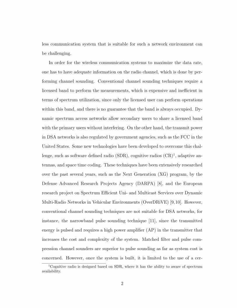
less communication system that is suitable for such a network environment can
be challenging.
In order for the wireless communication systems to maximize the data rate,
one has to have adequate information on the radio channel, which is done by per-
forming channel sounding. Conventional channel sounding techniques require a
licensed band to perform the measurements, which is expensive and inefficient in
terms of spectrum utilization, since only the licensed user can perform operations
within this band, and there is no guarantee that the band is always occupied. Dy-
namic spectrum access networks allow secondary users to share a licensed band
with the primary users without interfering. On the other hand, the transmit power
in DSA networks is also regulated by government agencies, such as the FCC in the
United States. Some new technologies have been developed to overcome this chal-
lenge, such as software defined radio (SDR), cognitive radios (CR)1, adaptive an-
tennas, and space time coding. These techniques have been extensively researched
over the past several years, such as the Next Generation (XG) program, by the
Defense Advanced Research Projects Agency (DARPA) [8], and the European
research project on Spectrum Efficient Uni- and Multicast Services over Dynamic
Multi-Radio Networks in Vehicular Environments (OverDRiVE) [9,10]. However,
conventional channel sounding techniques are not suitable for DSA networks, for
instance, the narrowband pulse sounding technique [11], since the transmitted
energy is pulsed and requires a high power amplifier (AP) in the transmitter that
increases the cost and complexity of the system. Matched filter and pulse com-
pression channel sounders are superior to pulse sounding as far as system cost is
concerned. However, once the system is built, it is limited to the use of a cer-
1Cognitive radio is designed based on SDR, where it has the ability to aware of spectrumavailability.
2

tain frequency. Hence, to design a channel sounder for DSA networks based on
cognitive radios is demanded.
Sliding correlator -based channel sounding techniques are frequency efficient in
terms of spectrum utilization since bandwidth compression allows us to perform a
wideband measurement with a relatively small bandwidth (slow A/D sample rate)
compared to pulse sounding. However, sliding correlator -based techniques still
require a licensed band and high transmit power to perform measurements. Thus,
operating a sliding correlator channel sounder in the DSA network is impractical.
Moreover, most of the conventional channel sounders are not SDR-based, which
means that once the system is built, the parameters can be changed, but with
difficulty. To operate in DSA networks, where frequent changes of transmission
and reception parameters are required, conventional channel sounders have to be
designed and implemented based on cognitive radios.
The existing problems motivate us to design an adaptive channel sounder for
DSA networks, in which the channel sounder can be operated at different center
frequencies depending on spectrum availability (either policy-based or measurement-
based) with extremely small transmit power relative to the conventional tech-
niques or adaptively varying transmit power without interfering with other users.
The swept time-delay cross correlation (STDCC) sounding technique is relatively
simple to implement, since it does not require a high sampling rate due to the
pulse compression technique, and only requires an m-sequence generator at the
transmitter and a cross-correlator at the receiver. Moreover, advanced signal
processing algorithms also enable us to eliminate the intermediate frequency op-
eration from the hardware domain to the software domain, which means that
the correlation and other signal processing can either be done by an end termi-
3

nal computer or by the on-board FPGA, depending on the requirements. By
combining the STDCC technique with the MC-DS-CDMA technique, called the
MC-DS-STDCC channel sounder, the transmit power is reduced by a factor of
the spreading sequence length. Moreover, the measurements can be employed at
different center frequencies with varying transmit power.
An alternative solution to the combination of spread spectrum and multicar-
rier techniques is to use the orthogonal frequency division multiplexing (OFDM)
technique as the channel sounding platform and utilize the user data to perform
channel sounding without introducing a dedicated sounding signal, such that in-
terference is minimized. The other advantage of this approach is that the sampling
rate requirement is not as high as that of the MC-DS-CDMA technique, since the
bandwidth is not traded for performance.
1.2 Implementation: A Whole New Story
Designing an algorithm may bring to light theoretical problems. One can
tackle those problems by making reasonable assumptions. However, implementing
a design will force us to face those problems and issues. For example, the sampling
rate of the device is restricted by the DAC and the ADC, while when designing
the algorithm we can assume that the DAC sampling rate is sufficient. Also,
the baseband bandwidth requirement of the design may be too ambitious for the
hardware device.
In this dissertation, the implementation issues will be assessed and studied
by observing the combination of the theoretical design and hardware capability.
The hardware platform for the implementation is the Universal Software Radio
Peripheral (USRP), which was developed by Ettus Research [12], and we use the
4

GNU Radio software to accomplish every single functionality of the system other
than the RF front end. This approach provides us many convenient features, such
as fast system reconfigurability, pure software implementation of algorithms, low
cost, etc. However, this approach is subject to the hardware capabilities when
considering the system design.
1.3 Current State-of-the-Art
Channel sounding techniques and devices have been used by researchers, wire-
less service providers, and spectrum regulation agencies for many years to capture
and study radio channel characteristics. In the early 1970s, a radio channel mea-
suring device based on sliding correlator was first developed by Cox [3–6]. This
was the first radio channel sounder that could measure both time and frequency
domain characteristics of a wireless channel, and it was also the first “wide-band”
channel sounder ever developed. The measurement was conducted at the 910
MHz band in an urban area of New York City, which later provided distributions
for multipath delay spread and average excess delay expected by wireless device
and systems. In 1991, Parsons named Cox’s channel sounder the swept time-delay
cross-correlator channel sounder [11]. He discovered the evolution of the slid-
ing correlation channel sounding techniques and also did a comparison between
different channel sounding techniques. In his paper, the channel sounders are
categorized into wide-band and narrow-band based on the width of the frequency
band of interest. The channel sounders are also divided into time and frequency
domain based on their functionality.
As wireless communication systems become more and more complicated, ac-
curate and comprehensive channel information becomes the key for the entire
5

system design. Depending on different applications, environment, and their op-
eration center frequencies, radio channel characteristics may vary from one to
another. Many researchers have conducted extensive measurements and analysis
for different radio channel environments and applications [13–28]. In addition to
radio channel measurement, statistical analysis on the data collected by the mea-
suring devices plays an important role in the entire system design. Not only does
statistical analysis help in understanding the radio channel, but it also provides a
way of predicting the channel [21,29–37].
Researchers have also shown that the performance in terms of delay resolution
and accuracy of the first proposed channel sounder by Cox can be improved by
designing a better sounding signal, applying signal processing on the collected
data, as well as by eliminating the unnecessary hardware (IF stage). With modern
communication technologies, the channel sounders can identify delay resolution
of sub second nano seconds for indoor environments [19, 33], as well as couple
hundreds of megahertz bandwidths [15]. G. Martin showed that the dynamic
range of a sliding correlator can be improved by a new algorithm [38]. It was also
shown in literature [23, 31, 39–44] that system performance can be improved by
designing a better sounding signal as well as by the use of signal processing.
1.4 Dissertation Contributions
This dissertation presents the following novel contributions:
• Characterized the user access randomness in both frequency and time do-
main. Addressed challenges in designing the channel sounding system for
the DSA network environment. Tasks needing to be solved were how to
6

perform channel sounding without interfering with other users, and how
to perform channel sounding efficiently when frequent frequency and time
switching is required.
• A multicarrier direct sequence spreading based channel sounding system
framework combined with the STDCC channel sounder, also termed as
MC-DS-STDCC, is presented. The MC-DS-STDCC utilizes direct sequence
spreading to minimize the interference to other users within the same fre-
quency band, and multicarrier modulation to achieve frequency agility. To
be more specific, each subcarrier is able to adjust the transmit power by
increasing or decreasing the spreading sequence length in order to satisfy
the power limit. Moreover, the use of spread spectrum also increases the
inherent processing gain of the system, and hence, the dynamic range of the
channel sounder is enlarged.
• In contrast to the MC-DS-STDCC channel sounding technique, the OFDM-
based channel sounding technique is focused on reducing the system com-
plexity, mainly sampling rate. The OFDM-based channel sounder has the
ability to use user data as the sounding signal, which eliminates the sounding
signal generator, and hence the system complexity is reduced. However, the
performance is directly related to the autocorrelation of the user transmit
data, that is, the optimal sounding signal is achieved when the data across
all subcarriers are equal to one. A tradeoff study is conducted by interpo-
lating performance loss versus randomness of the user data. On the other
hand, since the OFDM-based channel sounding technique uses user data as
the sounding signal, no extra interference will be introduced as long as the
7
user has permission to the frequency band. However, system performance
is traded off for system complexity.
• Channel sounder is a measurement device, and hence, it is only useful if im-
plemented. In this dissertation, implementation of the STDCC is presented
based on the USRP and GNU radio. Implementation of the MC-DS-STDCC
and OFDM-based channel sounder is outside the scope of this dissertation
because of hardware and software limitations; The USRP platform supports
a maximum bandwidth of 32 MHz by adopting a custom FPGA bitstream
file to bypass the bandpass filter built in on the daughter board. This band-
width limitation is the major obstacle to implementing the MC-DS-STDCC
channel sounder, which requires much higher bandwidth in order to perform
spread spectrum. Indoor experiments were conducted inside Nichols Hall in
Lawrence, KS. The experiment results were studied and analyzed.
1.5 Dissertation Organization
This dissertation is organized as follows: Chapter 2 discusses radio channel
environments including large-scale fading and small-scale fading. Mathematical
models of the radio channel are given, as well as the relationships between them.
The main focus of this chapter is radio channel characteristics in both time and fre-
quency domains. Several important channel parameters will be studied in detail,
such as channel impulse response, channel frequency response, doppler spread,
etc. The relationship and transform between time and frequency domain channel
characteristics are emphasized. In the last section, dynamic spectrum access net-
works is emphasized. The challenges and necessity in designing a channel sounding
8
system for such a network environment are addressed.
Chapter 3 consists of a literature survey of channel sounding techniques, each
of which is discussed in detail as to advantages and disadvantages, and the fun-
damentals of the sliding correlator theory and the STDCC technique. Problems
when utilizing conventional channel sounders in the DSA network environment
are addressed. The need for new channel sounding techniques for the dynamic
spectrum access networks is discovered, with emphasis on the challenges that
conventional channel sounding techniques encounter when being applied to such
network environments.
In Chapter 4, wideband channel sounding techniques are discussed. The pro-
posed technique is a combination of the multicarrier modulation technique and
the STDCC technique. Each technique is focused on solving a particular research
question. The MC-DS-STDCC technique is mainly designed for frequency-agile
and interference awareness as well as channel sounding performance. Drawbacks
of the MC-DS-STDCC technique are also presented, which become the motivation
for the OFDM-based channel sounding technique.
High sampling rate requirement and system complexity are the two major
drawbacks of the MC-DS-STDCC technique. In Chapter 5, an OFDM-based
channel sounding technique is presented in contrast to the previous technique.
The OFDM-based channel sounder does not require dedicated sounding signal
generation and signal processing, and hence, system complexity is reduced, and
the sampling rate required is relatively low, since time domain spreading is not
necessary. However, system performance is traded off for simplicity.
In Chapter 6, hardware and software implementation of the STDCC channel
sounder is presented. Implementation issues due to hardware and software limita-
9
tions are also discussed. Indoor channel measurements were conducted in Nichols
Hall, and measurement results were analyzed and studied.
The dissertation is concluded by future work and contributions in Chapter 7.
10

Chapter 2
Radio Propagation Channel
2.1 Fundamentals of Mobile Radio Channel
The mobile radio channel can be attributed to large-scale path loss channel
and small-scale fading (multipath fading channel). Large-scale path loss is used
to study electromagnetic wave propagation characteristics. As the name implies,
the propagation model is usually used to predict the mean signal strength for an
arbitrary transmitter-receiver separation. On the other hand, small-scale fading is
used to describe the rapid fluctuations of amplitudes, phases, or multipath delays
of a radio signal over a short period of time or travel distance, and hence the
large-scale path loss effects may be neglected when studying small-scale fading
channels. Unlike the deterministic feature of large-scale fading, small-scale fading
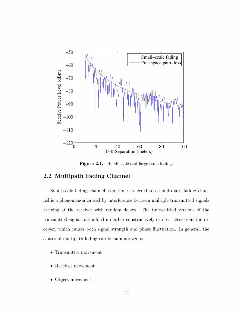
is a stochastic process that depends on many factors. Figure 2.1 illustrates a sim-
ulated small-scale fading and the more gradual large-scale average signal strength
variation versus transmitter-receiver separation. The average signal strength does
not change rapidly for a relatively short distance, hence, for studying small-scale
fading, the signal strength variations due to transmission distance is ignored.
11
0 20 40 60 80 100−120
−110
−100
−90
−80
−70
−60
−50
T−R Separation (meters)
Rec
eiv
e P
ow
er L
evel
(d
Bm
)
Small−scale fading
Free space path−loss
Figure 2.1. Small-scale and large-scale fading.
2.2 Multipath Fading Channel
Small-scale fading channel, sometimes referred to as multipath fading chan-
nel is a phenomenon caused by interference between multiple transmitted signals
arriving at the receiver with random delays. The time-shifted versions of the
transmitted signals are added up either constructively or destructively at the re-
ceiver, which causes both signal strength and phase fluctuation. In general, the
causes of multipath fading can be summarized as:
• Transmitter movement
• Receiver movement
• Object movement
12

• Signal reflected by objects.
Depending on the speed and direction of the movement, the multipath fading chan-
nel is defined as fast and slow fading channel, which is characterized by Doppler
shift [45]. Due to the random nature of the transmission channel, capturing and
modeling such a channel environment can be difficult. In the following sections,
the mobile radio channel is studied in three domains: temporal, frequency, and
space, with each having its own parameters.
2.3 Time and Frequency Domain Characteristics
2.3.1 Delay Spread, Power Delay Profile and rms Delay Spread
Delay spread, power delay profile, and rms delay spread are the most important
time domain characteristics of a wireless multipath fading channel. They are
indicators of the type of the channel, i.e., indoor channel, or outdoor channel,
and also frequency selective or nonselective. Let x (t) represent the transmitted
signal, y (t) the received signal, and h (t, τ) the impulse response of the time-
varying multipath fading channel. The variable t represents time variations due
to motion, whereas τ represents the channel multipath delay for a fixed value of
t. The received signal y (t) can be expressed as a convolution of the transmitted
signal x (t) with the channel impulse response:
y (t) =
∫ −∞∞
x (τ) · h (t, τ) · dτ = x (t)⊗ h (t, τ) . (2.1)
In order to model the channel impulse response, the multipath delay has to be
discrete, which means the delay axis τ is divided into equally spaced delay bins,
13

where each bin has a time delay width equal to τi+1 − τi = ∆τ . If we ignore
the propagation delay between the transmitter and the receiver, one can assume
that the first multipath component has delay of zero, τ0 = 0. Let N be the total
number of multipath components, so the maximum excess delay of the channel is
given by N∆τ . This channel is known as the tapped delay line model [46], which
is shown in Figure 2.2:
Z-1 Z-1 Z-1 Z-1. . .
. . .
x(t)
y(t)
h1(t) h
2(t) h
n-1(t) h
n(t)
Figure 2.2. Tapped delay line model.
In general, the time-varying nature of the channel can be modeled as a wide-
sense stationary (WSS) random process in the time variable t [47], and the at-
tenuation and the phase shift associated with different delays are assumed to be
uncorrelated, called the uncorrelated scattering (US) assumption [46, 47]. The
autocorrelation function of the time-varying channel is defined as [46]:
Rc (τ1, τ2,∆t) = E [c∗(τ1, t) · c (τ2, t+ ∆t)] , (2.2)
where Rc denotes the autocorrelation function of a WSS random process, E [·] rep-
resents the expectation operator, and c (τ, t) describes the time-varying, complex
lowpass-equivalent impulse response of the multipath fading channel. By applying
the US assumption, Equation (2.2) becomes:
Rc (τ1, τ2,∆t) = Rc (τ1,∆t) · δ (τ1 − τ2) . (2.3)
14

Equation (2.3) indicates that the autocorrelation function depends only on the
difference between τ1 and τ2. By replacing τ1 − τ2 with τ in the above equation,
Equation (2.2) can be written as:
Rc (τ,∆t) = E [c∗ (τ, t) · c (τ, t+ ∆t)] . (2.4)
Equation (2.4) is a time domain representation of the multipath fading channel. It
indicates that the autocorrelation function of the channel can be derived from the
expected value of the complex baseband impulse response. It would be helpful if
there existed a function that can simultaneously provide both time and frequency
domain description of the channel with respect to the delay variable τ and fre-
quency domain variable ω. It is obvious that such a function can be obtained by
applying the Fast Fourier Transform (FFT) on ∆t, which yields:
S (τ, ω) = F∆t [Rc(τ,∆t)] =
∫ ∞−∞
Rc (τ,∆t) · e−2πω∆t · d∆t, (2.5)
where F [·] denotes the Fourier transform with respect to ∆t. Function S(τ, ω) is
defined as the scattering function of the channel, which is the Fourier transform of
the channel autocorrelation function. Individually, the time and frequency domain
parameters can also be derived from the scattering function.
The power delay profile (PDP) is defined as the intensity of a signal received
through a multipath channel as a function of time delay. It can be calculated from
the complex impulse response c (τ, t) [45]:
p (τ) = E[| c (τ, t)2 |
]= Rc (τ, 0) , (2.6)
15

which is equal to the channel autocorrelation function evaluated at zero time
instance, Rc (τ,∆t) |∆t=0. Assuming the scattering function is known, the power
delay profile can be derived by averaging S (τ, ω) over the frequency domain:
∫ ∞−∞
∫ ∞−∞
S (τ, ω) =
∫ ∞−∞
∫ ∞−∞
Rc(τ,∆t) · e−j2πω∆t · d∆t · dτ
= Rc(τ, 0). (2.7)
Similarly, integrating the scattering function over the time domain yields the
frequency domain representation, Doppler spectrum:
S (ω) =
∫ ∞−∞
S (τ, ω) · dτ. (2.8)
−1
−0.5
0
0.5
1 00.5
11.5
2
0
0.005
0.01
0.015
0.02
Delay spreadNormalized Doppler shift
Am
pli
tud
e
Figure 2.3. Doppler shift vs. delay spread.
16

Figure 2.3 demonstrates the relationship between the delay spread, the Doppler
shift, and the amplitude of a multipath fading channel. The delay spread is
modeled by the exponential function e−τ , where the Doppler spectrum is based
on the Jakes model. The delay spread determines the bandwidth of the channel,
and the Doppler spectrum reflects the velocity of the mobile.
The relationship between the scattering function S (τ, ω) and the time and
frequency domain functions is summarized in Figure 2.4:
Figure 2.4. Relationship between scattering function, channel cor-relation functions, power delay profile, and Doppler power spectrum.
As shown in Figure 2.4, the time domain parameter power delay profile and the
frequency domain parameter frequency correlation function are a Fourier Trans-
form pair, so are the Doppler power spectrum and time correlation function. This
relationship provides us an additional path to obtaining the channel parameter
of one domain to another. Specifically, if one wants to get the frequency domain
17
channel parameter by using a time domain channel sounder, the FFT should be
applied. Given the development of efficient FFT algorithms and digital signal pro-
cessing (DSP) chips, implementing FFT on a hardware platform across all levels
becomes cheap and feasible. Moreover, this relationship also provides a funda-
mental support of the OFDM-based channel sounder, which will be discussed in
Chapter 5.
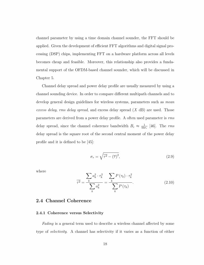
Channel delay spread and power delay profile are usually measured by using a
channel sounding device. In order to compare different multipath channels and to
develop general design guidelines for wireless systems, parameters such as mean
excess delay, rms delay spread, and excess delay spread (X dB) are used. Those
parameters are derived from a power delay profile. A often used parameter is rms
delay spread, since the channel coherence bandwidth Bc ≈ 150στ
[46]. The rms
delay spread is the square root of the second central moment of the power delay
profile and it is defined to be [45]:
στ =
√τ 2 − (τ)2, (2.9)
where
τ 2 =
∑k
a2k · τ 2
k∑k
a2k
=
∑k
P (τk) · τ 2k∑
k
P (τk). (2.10)
2.4 Channel Coherence
2.4.1 Coherence versus Selectivity
Fading is a general term used to describe a wireless channel affected by some
type of selectivity. A channel has selectivity if it varies as a function of either
18
time, frequency, or space. The opposite of selectivity is coherence. A channel has
coherence if it does not change as a function of time, frequency, or space over a
specified “window” of interest.
Indeed, wireless channels may be functions of time, frequency, and space. The
most fundamental concept in channel modeling is classifying the three possible
channel dependencies of time, frequency, and space as either coherent or selective
in order to keep track of these dependencies in the wireless channel. As described
in the previous sections, delay spread and channel coherence bandwidth are pa-
rameters which describe the time-dispersive nature of the channel. When the
time-varying nature of the channel is caused by either relative motion between
the mobile and base station, or by movement of objects in the channel. Doppler
spread and coherence time are the parameters which describe the channel.
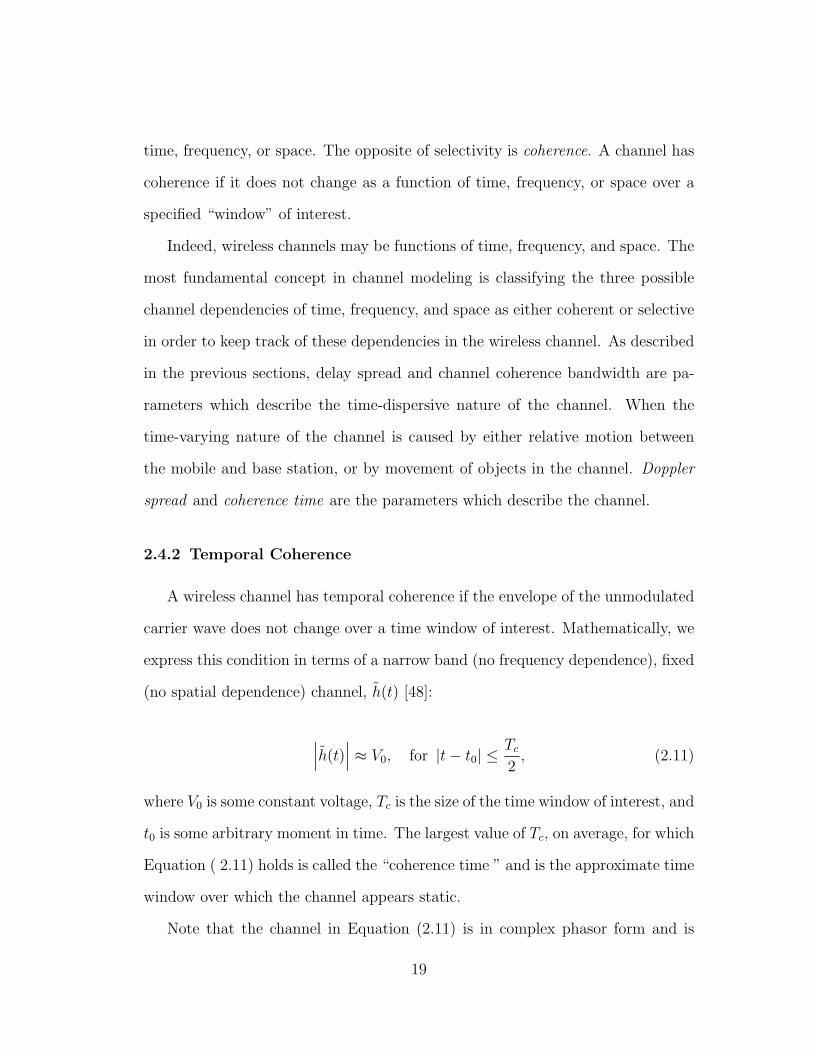
2.4.2 Temporal Coherence
A wireless channel has temporal coherence if the envelope of the unmodulated
carrier wave does not change over a time window of interest. Mathematically, we
express this condition in terms of a narrow band (no frequency dependence), fixed
(no spatial dependence) channel, h(t) [48]:
∣∣∣h(t)∣∣∣ ≈ V0, for |t− t0| ≤
Tc2, (2.11)
where V0 is some constant voltage, Tc is the size of the time window of interest, and
t0 is some arbitrary moment in time. The largest value of Tc, on average, for which
Equation ( 2.11) holds is called the “coherence time ” and is the approximate time
window over which the channel appears static.
Note that the channel in Equation (2.11) is in complex phasor form and is
19

independent of carrier frequency. Naturally, a transmitted wave will produce si-
nusoidal oscillations as a function of time, but the definition of temporal coherence
is concerned with the “envelope” of those oscillations. Temporal coherence is an
indication of how fast the channel response changes versus time, hence, the chan-
nel can be categorized into slow and fast fading. Slow and fast fading are relative
to the transmit symbol rate. If the channel impulse response does not vary during
one symbol period of the signal, the channel is considered as slow fading channel
to the signal, and vice versa.
To overcome the fast fading effect, one can transmit a signal with higher symbol
rate than the channel coherence time, that is, Tc ≤ Ts, where Tc represents the
channel coherence time, and Ts represents the symbol rate of the signal, so that
the channel impulse response is flat over one symbol period. In general, in order
to increase system throughput, we always transmit at high symbol rate. However,
this approach results in frequency domain fading, which will be discussed in the
next section.
2.4.3 Frequency Coherence
A wireless channel has frequency coherence if the magnitude of the carrier wave
does not change over a frequency window of interest. This window of interest is
the bandwidth of the transmitted signal. As we defined the time coherence of a
radio channel, the condition of frequency coherence in terms of the static, fixed
channel, h(f) [48] is:
∣∣∣h(f)∣∣∣ ≈ V0, for |fc − f | ≤
Bc
2, (2.12)
20

where V0 is again some constant amplitude, Bc is the size of the frequency window
of interest, and fc is the center carrier frequency.
The frequency coherence characteristic is described by the frequency correla-
tion function P (∆f), which represents the correlation between the channel re-
sponse to two narrowband signals with the frequencies f1 and f2. Channel coher-
ence bandwidth, Bc, is a statistical measure of the range of frequencies over which
the channel can pass all spectral components with approximately equal power and
linear phase. Channel coherence bandwidth reflects the correlation between two
frequency components across the frequency range of interest. Hence, the correla-
tion coefficient determines the coherence bandwidth. The greater the correlation
coefficient, the narrower the coherence bandwidth. Assuming that the correlation
between two frequency responses depends only on the frequency difference, that
is ∆f = f1 − f2, the normalized frequency correlation coefficient is then defined
as:
ρ∆f =E [H (f) ·H (f + ∆f)∗]
E[|H (f)|2
] . (2.13)
The frequency correlation function can be thought of as the transfer function of
the channel; hence, it is the inverse Fourier Transform of the channel impulse
response, and as a result, ∆f can be represented as: [46]:
∆f ≈ 1
τmax
, (2.14)
Equation (2.14) reveals the relationship between the power delay profile and the
frequency correlation function, that is, they are Fourier transform pairs. However,
a general relationship between the coherence bandwidth and rms delay spread
only exists for the specific channel models and must be derived from the actual
21
dispersion characteristics of the channels or statistical measurements and simula-
tion [45].
As mentioned in the previous section, transmitting a signal at high symbol
rate requires larger bandwidth, and hence if the channel coherence bandwidth
is smaller compared with the signal bandwidth, the received signal suffers from
frequency selectivity. Many techniques are available to compensate for the fad-
ing effects caused by frequency selectivity, one classic example being equalization.
Equalization is achieved by estimating the channel frequency response from the
distorted signal with various combining techniques [46]. Although equalization
can assist in improving signal quality and reducing bit error rate, it requires com-
plicated equalizer design at the receiver. When a communication system is to be
operated in a certain wireless environment, the channel characteristics need to be
acknowledged by performing channel sounding, which provides prior information
of the radio channel to the communication system designer.
2.5 Radio Channel Characteristics of the Dynamic
Spectrum Access Network Environment
As discussed in the previous sections, the characteristics of a radio channel
depend on many factors. Researchers have addressed factors that affect these
characteristics in both time and frequency domains. However, as the DSA network
comes into play, the radio channel can behave differently. For example, the channel
bandwidth can change from several megahertz to several hundred megahertz when
then channel type changes from outdoor to indoor. This phenomenon is caused
by the random access of the unlicensed users. In particular, the unlicensed users
22

can appear at a certain frequency band at any time as long as their activities
are legitimate. Figure 2.5 shows an example of the random access of unlicensed
user under licensed and unlicensed bands. The figure uses color scale to represent
2 4 6 8 10 12 14
2
4
6
8
10
12
14
Time Instance
Fre
qu
ecy
In
dex
0
2
4
6
8
10
12
PowerScale
Figure 2.5. Example of an unlicensed user appearing in a DSA net-work environment.
the transmit power level of a certain user in both time and frequency domains.
Zero on the power scale (in dark blue) shows that the slots are inaccessible by
the unlicensed user due to primary user reservation or power restriction. Different
color stands for different power level restrictions. In the time domain (x-axis in
the figure), the unlicensed user may occupy a certain band for a period of time
until the licensed users appear or other unlicensed users request to share the band.
That unlicensed user either has to wait until the band is available again, or hop
23

to another frequency band. This approach is suitable for applications that are
latency sensitive, such as file transfer, peer-to-peer, etc. Switching to a different
frequency band will guarantee continuity of connection at the cost of hardware
complexity, since the RF front end has to have the capability to switch between
center frequencies as well as be accommodative to different bandwidths.
The Unlicensed National Information Infrastructure (U-NII) radio bands and
the Industrial, Scientific and Medical (ISM) radio bands are two commonly used
unlicensed bands (IEEE 802.11), which cover a wide range of frequencies. Ta-
ble 2.1 lists the transmission parameters for each frequency range of the ISM and
U-NII bands.
Table 2.1. U-NII and ISM band specifications.
U-NIIa ISMb
Low Mid Worldwide Upper ISM
Band (GHz) 5.15-5.25 5.25-5.35 5.47-5.725 5.725-5.825 2.4-2.5
Power Limit 50 mW 250 mW 250 mW 1 W Varies
aU-NII is an FCC regulatory domain for 5 GHz wireless device, for complete reference pleasesee reference [49].
bISM bands listed here only indicate the most commonly used bands (WiFi band). Thecomplete ISM band definition can be found in [50].
For a cognitive radio device to operate in the frequency bands listed in Ta-
ble 2.1, not only must the device RF front end have the ability to tune accordingly,
but also the radio channel characteristics must vary as well. For example, the max-
imum Doppler shifts for a device operating at 5.15 and 5.85 GHz with velocity of
25 M/h are equal to 429.17 Hz and 487.5 Hz, respectively. In addition, the user
bandwidth may change according to the center frequency and maximum band-
width available. Hence, the user signal may suffer from different multipath fading
24

channels. For example, if the user signal bandwidth changes from 5 MHz to 500
KHz, and the channel coherence bandwidth remains 2 MHz, the multipath fading
channel for the user changes from frequency selective to frequency nonselective,
and it may change over time and frequency. This challenge requires cognitive
radios to have the ability to learn the radio channel and adjust their parameters
rapidly and adaptively before the radio channel changes.
In addition to the frequency and bandwidth restrictions, operating environ-
ment also plays a critical role in cognitive radio design. For an indoor environment,
the radio channel may be a frequency selective channel for the communication sys-
tem, while frequency nonselective when being operated outdoors. This is because
of the change in the maximum delay spread, which results in channel bandwidth
change. Moreover, the path loss factor varies from indoor to outdoor as well
as different channel models. Some devices may work for an indoor environment
but not for outdoors due to the change in channel type. In Chapter 6, channel
sounding experiments will be discussed in detail, the experiment results for both
indoors and outdoors will be shown. Briefly speaking, the USRP with 2.4 GHz
daughterboard works well for indoor applications. However, it fails to perform
channel sounding measurements for outdoor wireless channels.
2.6 Chapter Summary
In this chapter, conventional radio channel characteristics are presented with
focus on the time and frequency coherence of the multipath channel, since they are
the fundamentals of the signal processing portion of channel sounding techniques.
The relationship between time and frequency domain multipath channel charac-
teristics are presented in Figure 2.5. This relationship diagram reveals how the
25

parameters are interwoven together by the Fourier Transform. Key factors affect-
ing cognitive radio design are described, such as center frequency, user bandwidth,
velocity, and operating environment. Due to the network environment in which
cognitive radios are operated, channel sounding becomes especially critical, and
yet difficult to accomplish. Furthermore, the challenges to performing channel
sounding in a DSA network environment become the motivation of the research.
How to perform channel sounding efficiently, frequently, and quietly is to be an-
swered in the following chapters.
26
Chapter 3
Channel Sounding Techniques
Channel sounding is a technique that transmits a known signal to excite the
channel and observes the signal variations in amplitude and phase at the receiver.
It enables us to study and understand the radio channel characteristics. Early
channel sounding systems send a single tone (unmodulated CW carrier) to excite
the channel, and variations in power and phase are measured with a moving or a
stationary receiver. This is referred to as a narrow-band sounding technique [11].
When considering multipath fading channels, where two frequencies are correlated,
narrow-band sounding techniques become inefficient and impractical since a single
tone has to be transmitted at various frequencies of interest to be able to capture
the frequency and time coherence behavior of the channel [11].
In this section, a literature survey of existing channel sounding techniques is
provided, with the problems associated with each technique described. A widely
used technique, called STDCC, is emphasized.
27

3.1 Radio Channel Sounding
Radio channel sounding techniques, in general, can be categorized into narrow-
band and wideband sounding techniques, depending upon the transmit band-
width [11, 51]. Modern radio communication systems, such as WiFi and WiMax,
are normally operated in a wideband channel environment, where the desired sig-
nal is in the presence of several delayed versions of itself with random fading in
amplitude and phase offset. It can also be divided into time and frequency domain
channel sounding, where the time domain sounding is in the interest of capturing
the channel impulse response, and the frequency domain sounding aims to cap-
ture the frequency characteristics of the channel. Depending on the domain of
interest, the channel sounder design of the sounding signal and sounder structure
can be different. However, the time and frequency domain parameters are closely
related to each other, with several parameters being interderivable. For example,
the frequency correlation function can be obtained from a time domain channel
sounder by applying the Fast Fourier Transform (FFT) on the channel impulse
response. However, this operation requires additional processing. The frequency
domain measurement can also be obtained by using coherent measurement tech-
niques [52].
In order to capture the wideband channel parameters, such as the root mean
square (RMS) delay spread, the maximum delay spread, and the coherence band-
width, a sounding signal occupying wide bandwidth is required. Carrying out
narrowband measurements at a large range of frequencies of interest is expen-
sive in terms of hardware complexity, moreover the performance is limited by the
interference and hardware, since the hardware may be designed for a particular
28

center frequency, which may not be used for the others. Several wideband channel
sounding techniques have been devised, based on the periodic short duration pulse
approach, and the pulse compression technique [11]. Pulse compression-based
techniques, depending on different receiver structures, are realized by matched fil-
ter or cross correlation. Both methods will be discussed in details in the following
sections.
3.2 Periodic Pulse Channel Sounding
The principle behind the periodic pulse sounding technique is that a narrow
(short duration) pseudo-impulse is periodically transmitted to excite the chan-
nel (Figure 3.1), and the signal attenuation is measured by an envelop detector.
The impulse must be sufficiently narrow to ensure that the signal bandwidth is
larger than the channel coherence bandwidth to capture all the echoes. On the
other hand, two adjacent pulses have to be close enough observe the time-varying
behavior of each echo.
Tp
Tr
Figure 3.1. Periodic pulse sounding signal.
In Figure 3.1, Tp is the pulse duration, which represents the minimum identi-
fiable delay path resolution, and Tr is the pulse repetition period that is equal to
29

the maximum resolvable delay path. Each short pulse provides a ‘snapshot’ of the
multipath channel at a certain time instance. Combining a series of repetitions of
pulses together gives the channel behavior over the measurement duration.
The pulse sounding technique uses an envelope detection technique, which
means only the amplitude variations are recorded, and phase information is dis-
carded. Theoretically, the narrow pulse sounding technique is an ideal technique
if the pulse duration approaches zero, since the delay resolution is infinitely small.
However, the pulse sounding technique requires high unit transmit power to de-
tect weak signals, since all the energy is contained within the narrow pulse. High
peak-to-average power ratio (PAPR) is one of the major drawbacks of this tech-
nique, since it requires a large dynamic range of the transmit power amplifier in
order to guarantee accurate measurements. The cognitive radio and DSA enabled
devices are generally portable and compact, and large power consumption and
high sampling rate are avoided. The narrow pulse sounder is disqualified without
further modification.
3.3 Frequency Domain Channel Sounder: Chirp Sounder
As an alternative to the time domain channel sounder, we can estimate the
transfer function instead by using the chirp sounder. The main criterion for its
design is that is has a power spectrum |P (jω)|2, which is approximately constant
in the bandwidth of interest, and it allows interpretation of the measurement
result directly in the frequency domain. The time domain transmit waveform is
given as:
p(t) = exp
[2πj
(f0t+ ∆f
t2
2Tchirp
)]0 ≤ t ≤ Tchirp, (3.1)
30

consequently, the instantaneous frequency is:
f0 + ∆ft
Tchirp
, (3.2)
and thus has a linear relationship with time. The receiver filter requires a matched
filter to extract the transfer function. Intuitively, the chirp filter “sweeps” through
frequency range of interest, measuring different frequencies at different times. We
can improve the the sounding efficiency by performing measurement on different
frequencies at the same time. However, due to hardware costs, calibration issues,
etc., analog generation of p(t) using multiple oscillators to generate multiple fre-
quencies is not practical. Generating such signals digitally seems feasible, since
only a single oscillator is required, and the signal can be upconverted to the desired
passband.
3.4 Pulse Compression
The pulse compression is based on the theory of linear systems [11, 53]. It
provides a way to reduce the sampling rate by compressing the wideband signal
bandwidth. The measurement time is increased as a tradeoff due to the extra
processing time of pulse compression. If we consider the white noise n(t) as the
input to a linear system with impulse response of h(t), the output signal s(t) is
the convolution of n(t) and h(t):
s(t) =
∫h(τ) · n(t− τ)dτ. (3.3)
31
If the output signal s(t) is cross correlated with a delayed version of the input,
the resulting cross correlation coefficient is proportional to the impulse response
of the system h(τ):
E [s (t) · n∗ (t− τ)] = E
[∫h(ξ) · n(t− ξ) · n∗(t− τ)dξ
]=
∫h (ξ) ·Rn (τ − ξ) dξ, (3.4)
where Rn(τ) is the autocorrelation function of white noise n(τ), which is equal to
the single-sided noise power spectral density, N0. Hence, Equation (3.4) can be
expressed as:
E [s (t) · n∗ (t− τ)] = N0 · h (τ) . (3.5)
Equation (3.5) indicates that the impulse response of a linear system can be
obtained using white noise as the input, and correlation technique. Generating
white noise is unrealistic in practical applications. However, pseudo-random (PN)
sequences have been studied and researched due to its noise-like characteristic [54].
To be explicit, the autocorrelation and cross correlation functions of the maximum
length PN sequence (m-sequence) are periodic and binary valued, and the m-
sequence is easy to generate with the linear shift feedback registers (LSFR). The
m-sequence is also balanced, meaning that the number of ones is one greater than
the number of zeros in each period of the sequence, which can limit the degree of
carrier suppression [55]. Another advantage of using PN sequences is the inherent
processing gain achieved by the cross correlation process, which will be discussed
in detail in Section 3.5.2.2.
32
3.4.1 Convolution Matched Filter
The convolution matched filter technique falls into the pulse compression cate-
gory. It uses a filter that matches the sounding signal to achieve pulse compression.
A commonly used matched filter is the surface acoustic wave (SAW) filter. The
SAW filter on the receive side is matched to the transmit m-sequence, which re-
duces the hardware cost of the system, since it eliminates the generation of the
identical m-sequence at the receiver. The output of the matched filter is a series
of snapshots of channel impulse responses, which allows the system to operate
in real time [11]. However, the performance of the SAW filter is limited by the
devices. When the m-sequence length is long, it is difficult to generate spurious
acoustic signals. Imperfect surface acoustic waves degrade the sounder perfor-
mance in terms of delay resolution and dynamic range [53]. Some other effects
can also cause sensitivity degradation, such as temperature, filter materials, etc.
In general, SAW filters are designed for a particular center frequency with a cer-
tain bandwidth. The hardware cost constrains the application of SAW filters in
DSA networks, where operation frequency and bandwidth may change in random
manners.
3.5 The STDCC Technique
The STDCC channel sounding technique is the most widely used technique by
researchers and industry due to the outstanding features [4, 11, 53]. First, it can
perform channel sounding over a wide bandwidth, which is suitable for modern
wideband communications. Second, it reduces the sampling rate at the receiver
compared with the matched filter and chirp sounders. Matched filter and chirp
33

sounder require sampling at the Nyquist rate where the STDCC only uses a single
sample at the maximum of the autocorrelation function. Third, the STDCC does
not suffer from high PAPR, because of the use of the spread spectrum technique.
Last but not least, signal processing can either be done by the hardware or software
depending on the requirement. If realtime channel sounding is required, the signal
processing algorithms can be uploaded to the FPGA, so that realtime channel
impulse responses can be observed. Off-line signal processing saves expense on
board memory, and one can develop complicated signal processing algorithms to
obtain better channel sounding performance.
3.5.1 Overview
The STDCC is based on the sliding correlator theory [4]. It is simple to imple-
ment and does not require a high sampling rate compared with conventional cor-
relative channel sounders [11]. Conventional correlative channel sounders sample
at the Nyquist rate, while the STDCC takes one sample value for each m-sequence
at the maximum amplitude of the autocorrelation function. The position of the
maximum peak of the autocorrelation function changes for each transmission cycle
of the m-sequence. STDCC pulse compression is done by correlating the received
sequence with an identical sequence clocked at a slightly lower rate. The difference
in chip rate is called slip rate, which is defined as:
fslip = fTx − fRx. (3.6)
The difference in chip rate results in different time bases between the transmit-
ted and the received sequences. The slower sequence (received sequence) will be
34

aligned with the transmitted sequence again after a duration:
Tslip =1
fslip
. (3.7)
The time domain representation, Kscale gives us the number of samples for a single
impulse response h(τi), and it is defined as:
Kscale =fTx
fslip
>> 1, (3.8)
the larger the number of samples, the better the delay resolution. On the down
side, the measurement duration is also increased by a factor of Kscale. The trade-
off between measurement time and delay resolution needs to be considered for
different radio channel environments. However, the sliding correlator can be sub-
stituted by a stepping correlator [40,56,57] in order to use digital signal processing
techniques for improving the system performance. The STDCC transmitter and
receiver schematics are shown in Figure 3.2. The schematic shown in Figure 3.2 is
oversimplified, as it does not contain all the components, for example the interme-
diate frequency (IF) stage. The IF frequency at the transmitter employed by Cox
is 10 MHz [3]. Both the Kansas University agile radio (KUAR) [58] and universal
software radio peripheral (USRP) offer baseband bandwidth greater than 10 MHz.
For the implementation consideration, we do not have to have the IF block as long
as the sounding signal bandwidth is less than the maximum baseband bandwidth
that the hardware can offer. The transmitter consists of a Pseudo-random Binary
Sequence (PRBS) and a Radio Frequency (RF) end. An m-sequence generator is
driven by a local clock with varying clock rate depending on the requirement. The
m-sequence is then modulated and fed into the RF end and transmitted. At the
35

RF End
PRBS Generator
M-sequence
GeneratorBPSK Modulation
cf
amp
fTx
(a) STDCC Transmitter
PRBS Generator
M-sequence
GeneratorBPSK Modulation
fRx=fTx- f
RF Front End
90o Hybrid
Correlator
Correlator
90
0
I( )
Q( )
)()( 22 QIEnvelop
(b) STDCC Receiver
Figure 3.2. Schematic of the STDCC transceiver.
receiver end, the received signal is filtered and passed through a low noise ampli-
fier (LNA), the inphase (I) and the quadrature (Q) of the signal are individually
correlated with an identical PRBS signal except that the m-sequence generator
is clocked at a slightly lower rate. The schematic shown previously provides a
full hardware implementation of the STDCC. If a software and hardware hybrid
implementation is used, anything beyond the RF front end can be implemented
in the software to minimize the hardware scale.
3.5.2 System Parameters
In this section, several critical system parameters of the STDCC channel
sounder are presented. The relationship between the parameters and the system
36
performance is addressed.
3.5.2.1 Multipath Resolution
The multipath resolution capability of the channel sounder is summarized as:
the maximum delay resolution and the minimum identifiable multipath resolution.
The maximum delay resolution is defined as the capability to detect the max-
imum unambiguous multipath component by the sounder, which is a function of
the m-sequence length. The maximum path delay that can be measured by the
sounder is smaller than L/Rc, where Rc is the m-sequence clock rate, and L is the
sequence length (in chips). The sequence period L/Rc has to be greater than the
τmax to ensure that no echoes are neglected.
The minimum identifiable multipath resolution is the difference between two
adjacent multipath components, and it is a function of the m-sequence chip rate
as well as the slip rate fslip.
3.5.2.2 Dynamic Range
The dynamic range, in decibels, is defined as the ratio of the magnitude of the
correlation peak and the magnitude of the maximum spurious correlation value:
DR = 10 log10(L2), (3.9)
where L is the m-sequence length [53]. It represents the ability to detect weak
signals. The ideal dynamic range for m-sequence with L varying from 127 to
2047 is shown in Table 3.1. For an AWGN channel, the dynamic range can be
represented as the ratio of the peak power level and the noise power level, and as
37
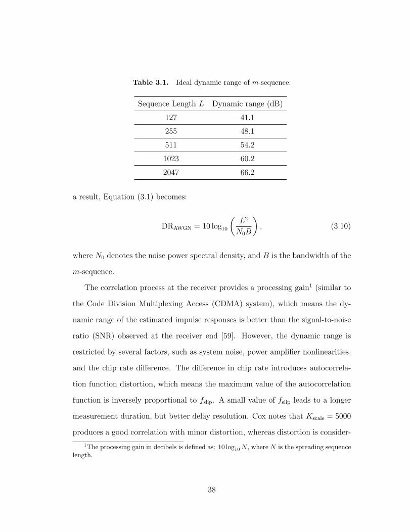
Table 3.1. Ideal dynamic range of m-sequence.
Sequence Length L Dynamic range (dB)
127 41.1
255 48.1
511 54.2
1023 60.2
2047 66.2
a result, Equation (3.1) becomes:
DRAWGN = 10 log10
(L2
N0B
), (3.10)
where N0 denotes the noise power spectral density, and B is the bandwidth of the
m-sequence.
The correlation process at the receiver provides a processing gain1 (similar to
the Code Division Multiplexing Access (CDMA) system), which means the dy-
namic range of the estimated impulse responses is better than the signal-to-noise
ratio (SNR) observed at the receiver end [59]. However, the dynamic range is
restricted by several factors, such as system noise, power amplifier nonlinearities,
and the chip rate difference. The difference in chip rate introduces autocorrela-
tion function distortion, which means the maximum value of the autocorrelation
function is inversely proportional to fslip. A small value of fslip leads to a longer
measurement duration, but better delay resolution. Cox notes that Kscale = 5000
produces a good correlation with minor distortion, whereas distortion is consider-
1The processing gain in decibels is defined as: 10 log10N , where N is the spreading sequencelength.
38
able when Kscale = 1000 [3]. Martin discusses the relationship between achievable
dynamic range and correlation noise by using a novel sliding correlation algorithm
in the correlation process, and quantifies dynamic range as a function of the ratio
of Kscale (time scaling factor) and L (the m-sequence length). This contribution
provides us a systematic method of designing sliding correlators [38].
3.5.2.3 Time Scaling Factor
As mentioned in the previous section, a large time scaling factor provides good
minimum identifiable delay performance and minimum distortion, but also results
in longer correlation time and larger memory sizes to store the data. The choice of
the time scaling factor is dependent only on the requirement and channel environ-
ment. For example, for outdoor channel sounding, the number of reflected paths
and maximum delay are substantially larger than those of indoor environments,
but the minimum delay is on the order of microseconds. Such an radio channel
would require a channel sounder with longer sounding sequences, and slower chip
rate and vice versa for an indoor channel. However, both outdoor and indoor
channel sounding always need a larger dynamic range, which is directly related to
the sequence length.
3.5.2.4 Doppler-shift Resolution
The Doppler-shift resolution is a function of the transmitter and receiver ve-
locity (v), carrier frequency (fc), m-sequence length (L), clock rate (τc), and time
scaling factor (Kscale). The relationship between these values can be summarized
as follows:
39

• Maximum Doppler shift experienced by a moving receiver with velocity v is:
fD =v · fc
c, (3.11)
where c = 3× 10⁸m/s is the free space velocity of electromagnetic waves.
• The maximum Doppler shift that can be measured by STDCC is given by:
fD =1
2Kscale · L · τc
. (3.12)
Inserting Equation (3.12) into Equation (3.11) yields:
v =c
2Kscale · L · τc · fc
. (3.13)
Equation (3.13) indicates that v is inversely proportional to the m-sequence
length for fixed Kscale, τc, and fc:
v ∝ 1
L. (3.14)
The derivation above leads to a new problem of finding the tradeoff between
delay resolution and Doppler-shift resolution. Longer m-sequence provides better
minimum identifiable delay resolution, but sacrifices the Doppler-shift resolution.
For situations in which both transmitter and receiver are stationary, the Doppler-
shift resolution can be ignored, such that better dynamic range performance can
be achieved.
40

3.6 Frequency Domain Characterization
The frequency correlation function is a measure of the correlation between two
spaced carrier frequencies. This function is generated from the values of P (τi)
through FFT techniques [60]. The coherence bandwidth, defined as the maximum
frequency difference for which two signals have a specified value of correlation,
is a frequency domain parameter that is used for assessing the performance of
various modulation or diversity techniques. No definitive value of correlation has
been established for the specification of coherence bandwidth. However, channel
coherence bandwidth values of 0.9 (B0.9) and 0.5 (B0.5) are the two most widely
used values [45]. The resolution in the frequency domain, however, is related
to the pulse repetition frequency (PRF) of the spread spectrum sounding signal,
which is defined as:
PRF =1
Lτ0
, (3.15)
e.g., for L = 127 and τ0 = 0.1 µs, the PRF is 78.74 kHz. If the frequency resolution
is not sufficient, detail may be lost in the estimation of the frequency correlation
function resulting in erroneous values for B0.9 and B0.5. In essence, this is the
same problem that afflicts the spaced-tone sounding techniques.
One obvious method of counteracting this problem is to increase the length
of the m-sequence, thereby maintaining the same time resolution. However, the
drawback for adopting this approach, as discussed previously, limits the maximum
practical value of m.
An alternative and more elegant solution has been proposed by Haese [20].
Since it is assumed that all distinguishable echoes in the power-delay profile occur
within a certain time delay window, if the length of the m-sequence is doubled,
41

the new power-delay profile will contain exactly the same information up to a
delay of 12.7 µs with only the system noise floor extending to 25.4 µs. However,
the frequency resolution capability will improve from 78.74 kHz to 39.37 kHz.
In practice, therefore, the frequency resolution capability can be improved by
increasing the length of the time delay window off-line, i.e., after completion of
the field trials, by taking the system noise floor and extending it in time, prior to
using the FFT.
As opposed to the case where m is increased, the only penalty of increasing
the length of the time delay window off-line is the increased time of computation.
3.7 Chapter Summary
In this chapter, an overview of the radio channel sounding techniques is pro-
vided. Both the advantages and disadvantages of each technique were outlined.
The reasons why the STDCC channel sounding technique is chosen as the pro-
totype technique for DSA networks are addressed. The swept time-delay cross
correlation technique was emphasized, system parameters were discussed from a
design point of view. The inherent processing gain makes STDCC the nearest to
optimum sounding technique for DSA networks. However, some necessary mod-
ifications to the STDCC systems are required before applying to DSA networks,
such as transmit power, sounding efficiency, which will be discussed more in detail
in later chapters.
42
Chapter 4
Multi-carrier Swept Time Delay
Cross Correlation Channel
Sounder
Multicarrier modulation (MCM) techniques are promising candidates for DSA
networks due to their spectrum utilization efficiency and robustness. Two ma-
jor types of MCM techniques are Orthogonal Frequency Division Multiplexing
(OFDM) and Multicarrier Code Division Multiple Access (MC-CDMA). For each
type, there are many different versions in terms of implementation, especially
for the MC-CDMA systems. Depending on how the spreading is achieved, MC-
CDMA systems can be divided into Multicarrier Direct Sequence Code Division
Multiple Access (MC-DS-CDMA) and MC-CDMA (in general). If the spreading
is performed in the time domain, the system is called MC-DS-CDMA, while in
contrast, the system is named MC-CDMA for frequency domain spreading.
Both systems have their own advantages and disadvantages, which have been
43

fully studied in [61]. The motivation of collaborating multicarrier system and
STDCC system is to improve the channel sounding efficiency, since with MCM
techniques, one can operate at different center frequencies simultaneously. In
addition, a Direct Sequence (DS) technique allows us to change the signal power
by varying the spreading sequence length. This property fits in the DSA network
perfectly, where secondary users can only have access to certain bands at certain
time with limited power based on FCC regulations.
In this chapter, a novel channel sounding technique, named MC-DS-STDCC,
is introduced, starting by a brief introduction to the MC-DS-CDMA system, and
followed by the MC-DS-STDCC system structure. A comparison study between
conventional STDCC and MC-DS-STDCC is conducted, including simulation re-
sults on channel sounding performance and mathematical analysis. Further issues
of the MC-DS-STDCC is addressed.
4.1 MC-DS-CDMA System
In this dissertation, the MC-DS-CDMA system is not only considered as a data
transmission system, but also as a platform for the STDCC technique. Figure 4.1
shows the MC-DS-CDMA transceiver block diagrams.
In Figure 4.1, x(t) and s(t) stand for the input and output signal of the trans-
mitter. Similarly, x′(t) and s′(t) are the input and the output of the receiver. N
represents the total number of subcarriers, which is also the FFT size. T0 is the
input signal x(t) symbol duration, Ci, i = 1 . . . N is the spreading code space, and
the codes do not have to be orthogonal in this case, since the time domain signal is
not summed up before transmit. The value Mi, i = 1 . . . N , represents the length
of each individual spreading sequence. Generally, they all have the same length,
44

S/P
C1
C2
CN
IFF
T
P/S
MP
SK
Mo
du
lato
r
)(tx )(ts
spreading
0T
N
T0
N
T0
N
T0
1
0M
N
T
2
0M
N
T
NM
N
T0
(a) MC-CDMA Transmitter
S/P)(' ts
FF
T
despreading
*1C
*2C
*N
C
P/S
MP
SK
Dem
od
ula
tor
)(' tx
(b) MC-CDMA Receiver
Figure 4.1. MC-CDMA transceiver.
but it is possible to use various length spreading sequences to achieve signal power
adjustment for each subcarrier.
On the transmitter side, a serial data sequence is first M-PSK modulated and
then converted into parallel before being fed into the spreading and the inverse
fast Fourier Transform (IFFT) blocks. After serial to parallel (S/P) conversion,
data on each subcarrier is multiplied with corresponding spreading sequence, Ci,
and then the signal on individual subcarrier is modulated onto different carrier
45

frequencies by the IFFT. The parallel signal is serialized and transmitted. The
receiver performs the reverse operation, except that the despreading process uses
the complex conjugate version of the spreading sequence. The schematic does not
include Cyclic Prefix (CP) block, which is used to eliminate the effects of Inter-
Symbol Interference (ISI). Since we are employing the MC-DS-CDMA system as
a channel sounding system, we are interested in capturing the entire channel be-
havior. Thus, we do not employ CP, since all the channel information is contained
in the distorted signal.
4.2 Combined STDCC MC-DS-CDMA Implementation
The proposed technique employs multicarrier direct sequence spread spectrum
modulation and STDCC channel sounding to tailor the channel sounding signal
transmit power level across frequency, thus minimizing the amount of interference
introduced per subband. Each subcarrier in an MC-DS-CDMA system is consid-
ered as a branch, on which a complete STDCC system is operating. The system is
similar to a conventional MC-DS-CDMA system, except some changes are made to
integrate the STDCC system. MC-CDMA systems have various implementations
depending on which domain the spreading is performed. Time domain spreading
can minimize the interference caused to other subcarriers and users at cost of high
sampling rate. Frequency domain spreading enhances the immunity to frequency
errors, which is critical to any type of multicarrier system. Since reducing interfer-
ence to the interference tolerance of other users is one of our main objectives, the
MC-DS-CDMA system is selected to be collaborated with the STDCC channel
sounding technique. The transmitter and receiver block diagrams are illustrated
in Figure 4.2.
46

PRBS
Generator
OFDM
Modulator
(IFFT)
.
.
.
P/S
Copie
r
Zer
o-p
addin
g.
.
.
C1
C2
CN
spreadingMi
to receiver
s(t)
(a) MC-DS-STDCC Transmitter
OFDM
Demodulator
(FFT)
.
.
.
Plo
t an
d o
ther
Est
imati
on
S/P
Zero
-rem
ov
al
.
.
.
cross-correlation
Mi
to receiver
(t)
PRBS
Generator
.
.
.
(b) MC-DS-STDCC Receiver
Figure 4.2. MC-DS-STDCC transceiver.
47

On the transmitter side, Figure 4.2(a), a pseudo-random binary sequence
(PRBS) of data rate Rb is copied N times, where N is the number of subcar-
riers corresponding to different frequency bands, and propagated in parallel such
that the data rate of each subcarrier signal is the same as the original signal.
The subcarrier signals are then spread in the time domain with an independent
spreading code. The selection of the spreading code depends on the system re-
quirement. The data rate for each subcarrier after spreading becomes the chip
rate MiRb, where Mi is the spreading sequence length of the ith subcarrier. Note
that Mi could be different for each subcarrier depending on the power level limit
of each frequency band or interference tolerance.
In this dissertation, the Orthogonal Variable Spreading Factor (OVSF) codes
and m-sequence are studied and compared as the spreading codes for the sounder.
OVSF codes are recommended for Wideband-CDMA (W-CDMA) systems [62].
One important property of OVSF codes is that the orthogonality between codes
is guaranteed regardless of spreading factors, which reduces the intercarrier inter-
ference. It was first designed to achieve various symbol rates for different users in
W-CDMA systems [29,63]. This property of the OVSF codes guarantees orthog-
onality between codes for the case where spreading codes with different lengths
are used.
Due to the chip rate difference after spreading, shorter output sequences are
zero-padded to compensate for the chip rate differences with respect to the largest
spreading sequence length Mm = maxMi, such that all the output sequences are
aligned in time before the IFFT operation. Hence, the chip rate is equal to MmRb
for each subcarrier signal. Extra information on the power level limit for each
frequency band also needs to be transmitted to the receiver. This information
48
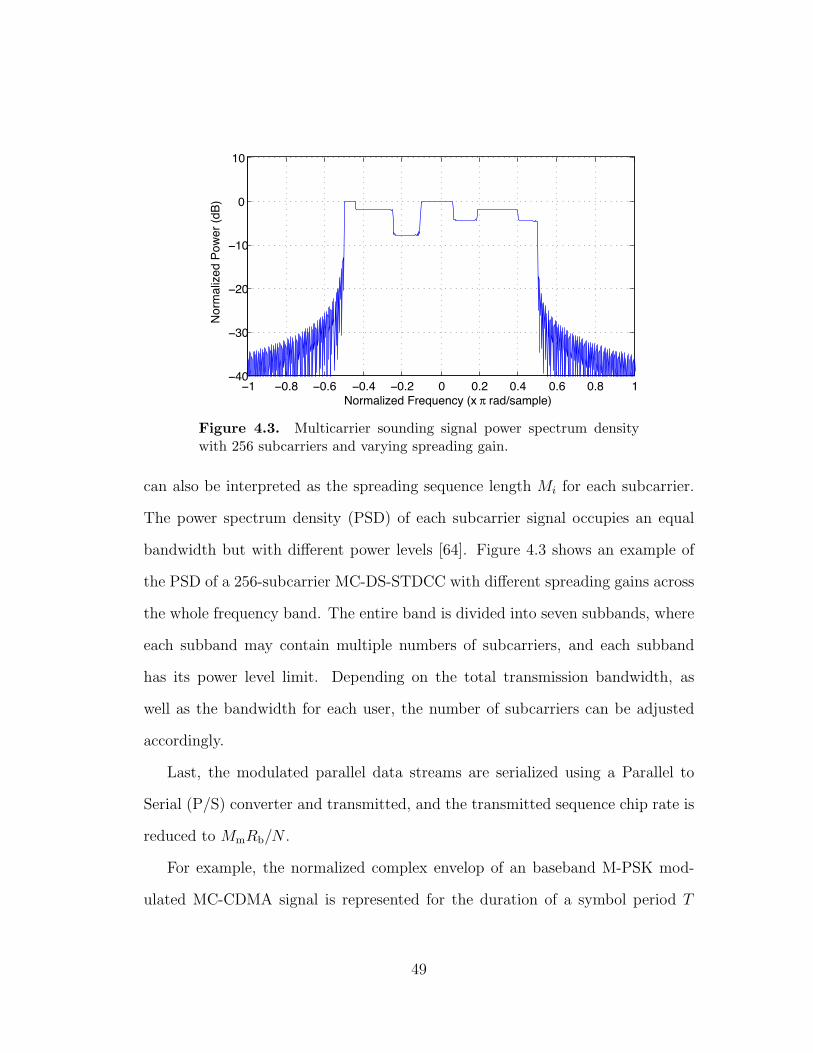
−1 −0.8 −0.6 −0.4 −0.2 0 0.2 0.4 0.6 0.8 1−40
−30
−20
−10
0
10
Normalized Frequency (x π rad/sample)
Norm
aliz
ed P
ow
er
(dB
)
Figure 4.3. Multicarrier sounding signal power spectrum densitywith 256 subcarriers and varying spreading gain.
can also be interpreted as the spreading sequence length Mi for each subcarrier.
The power spectrum density (PSD) of each subcarrier signal occupies an equal
bandwidth but with different power levels [64]. Figure 4.3 shows an example of
the PSD of a 256-subcarrier MC-DS-STDCC with different spreading gains across
the whole frequency band. The entire band is divided into seven subbands, where
each subband may contain multiple numbers of subcarriers, and each subband
has its power level limit. Depending on the total transmission bandwidth, as
well as the bandwidth for each user, the number of subcarriers can be adjusted
accordingly.
Last, the modulated parallel data streams are serialized using a Parallel to
Serial (P/S) converter and transmitted, and the transmitted sequence chip rate is
reduced to MmRb/N .
For example, the normalized complex envelop of an baseband M-PSK mod-
ulated MC-CDMA signal is represented for the duration of a symbol period T
49
as:
s(t) =1√N
N−1∑n=0
Mn−1∑m=0
bn · cn [m] · ej2πFnRnbmt,
where N is the number of subcarriers, Mn represents spreading sequence length
of each subcarrier, bn is the information bit of the nth subcarrier, and cn[m] is
the mth chip of the spreading sequence associated with the information bit on the
nth subcarrier. The square bracket [·] denotes the discrete index of the spreading
sequence, since Mn is a variable according to different subcarriers, and the length
of cn[m] is also different for each subcarrier. For calculating the envelope power
of the signal, we only consider nonzero values, which means we only consider
the elements satisfying |cn[m]| = 1. Fn is defined as the subcarrier separation
parameter, in other words, it is the ratio between the spreading sequence length
(spreading gain) and the number of subcarriers: Fn = Mn/N [65]. When F =
1, the subcarrier separation is the symbol rate Rb, the MC-DS-CDMA signal
spectrum has the same shape, as in an MC-CDMA system. When F is a variable,
the signal spectrum is no longer the same. To maintain the subcarrier separation
constant, but vary the signal power on each subcarrier, the symbol rate Rb is also
changed accordingly by zero-padding, and those two variables are represented as
Fn and Rnb.
The received signal is converted into N parallel data streams and fed into each
subcarrier. The extra zeros are removed based on information Mi before FFT
demodulation. The cross-correlation operation is done on a subcarrier basis, where
the demodulated signal is cross-correlated with an individual PRBS signal at chip
rate of MmRb. The PRBS signal used at the receiver is obtained by spreading
the output of an identical PRBS generator with respect to the spreading sequence
length for each subcarrier.
50

At the receiver, shown in Figure 4.2, the distorted signal is parallized into N
streams, and the time domain signal is then converted to the frequency domain
by FFT demodulation. The cross-correlation process is done on a subcarrier ba-
sis, since each branch carries a complete STDCC unit. After the cross-correlation,
each branch gives a series of channel impulse responses for the center frequency as-
sociated with it, and they are expressed as hi(τ), i = 1 . . . N . The cross-correlation
process produces a direct estimation of the time domain channel response. The
transfer function can be obtained by applying FFT on the power delay profile
(PDP) on each branch. Note that the receiver does not despread the received sig-
nal prior to cross-correlation in order to maintain a high sampling rate such that
the delay resolution is improved. Moreover, despreading the received signal will
discard the desired channel information. The disadvantage is that the autocorre-
lation property of the m-sequence is ruined. However, channel sounding accuracy
can still be guaranteed if the spreading sequence length is properly selected. The
locally generated m-sequence is correlated with the distorted spread spectrum sig-
nal to recover the channel impulse response. The impact on the performance will
be quantified in the later section.
4.2.1 Channel Impulse Response Estimation
Intuitively, it is possible to obtain the channel frequency response by taking
advantage of the FFT operation built in the MC-CDMA system. However, one
common assumption for multicarrier modulation systems, i.e., OFDM and MC-
CDMA, is that the carrier separation should be large enough to make sure the
signal on each subcarrier undergoes the independent fading. In contrast, for the
MC-DS-STDCC system, the frequency response might only be obtained under the
51
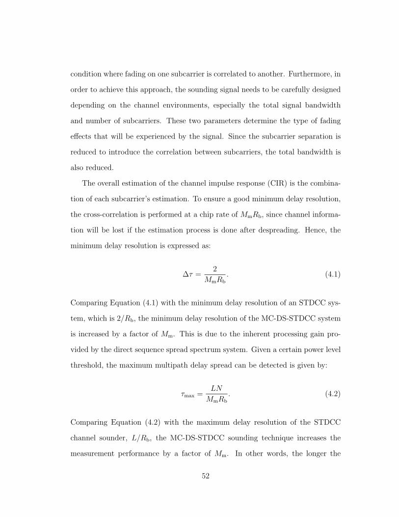
condition where fading on one subcarrier is correlated to another. Furthermore, in
order to achieve this approach, the sounding signal needs to be carefully designed
depending on the channel environments, especially the total signal bandwidth
and number of subcarriers. These two parameters determine the type of fading
effects that will be experienced by the signal. Since the subcarrier separation is
reduced to introduce the correlation between subcarriers, the total bandwidth is
also reduced.
The overall estimation of the channel impulse response (CIR) is the combina-
tion of each subcarrier’s estimation. To ensure a good minimum delay resolution,
the cross-correlation is performed at a chip rate of MmRb, since channel informa-
tion will be lost if the estimation process is done after despreading. Hence, the
minimum delay resolution is expressed as:
∆τ =2
MmRb
. (4.1)
Comparing Equation (4.1) with the minimum delay resolution of an STDCC sys-
tem, which is 2/Rb, the minimum delay resolution of the MC-DS-STDCC system
is increased by a factor of Mm. This is due to the inherent processing gain pro-
vided by the direct sequence spread spectrum system. Given a certain power level
threshold, the maximum multipath delay spread can be detected is given by:
τmax =LN
MmRb
. (4.2)
Comparing Equation (4.2) with the maximum delay resolution of the STDCC
channel sounder, L/Rb, the MC-DS-STDCC sounding technique increases the
measurement performance by a factor of Mm. In other words, the longer the
52

spreading sequence, the better the performance. However, this approach is at the
cost of high sampling rate and system complexity. As discussed in Chapter 3,
the PRBS used at the receiver is generated locally, which introduces the potential
issue of synchronization. If the received signal and locally generated signal are
not synchronized in time before they correlate with each other, the estimation will
result in a time-shifted version of the channel impulse response. However, this can
be compensated for by estimating the phase rotation of the out-of-phase signal.
4.2.2 Dynamic Range Performance
Ideally, the autocorrelation function (ACF) of an m-sequence is a near-optimal
approximation to a train of Kronecker delta function.1 Spreading the sounding
signal (m-sequence) at the transmitter increases delay resolution. However, the
autocorrelation function of the sequence after spreading is no longer Kronecker
delta like. This is because the insertion of the spreading sequence partially breaks
the property of the original m-sequence, which results in a “noisy” autocorrelation
function. However, the autocorrelation function of the resulting sequence can be
calculated by using the partial autocorrelation property of the m-sequence [66].
It is well known that the periodic autocorrelation function of an m-sequence b is
given by [67]:
θb(k) =
1, k = lN
− 1N, k 6= lN
, (4.3)
where θb(k) denotes the value of the autocorrelation function at the kth lag , and
N represents the sequence period and l is an integer. Note that Equation (4.3)
1Kronecker delta function δ is defined as: δi =
1, if i = 00, if i 6= 0 .
53
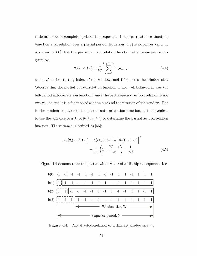
is defined over a complete cycle of the sequence. If the correlation estimate is
based on a correlation over a partial period, Equation (4.3) is no longer valid. It
is shown in [66] that the partial autocorrelation function of an m-sequence b is
given by:
θb(k, k′,W ) =
1
W
k′+W−1∑m=k′
amam+k, (4.4)
where k′ is the starting index of the window, and W denotes the window size.
Observe that the partial autocorrelation function is not well behaved as was the
full-period autocorrelation function, since the partial-period autocorrelation is not
two-valued and it is a function of window size and the position of the window. Due
to the random behavior of the partial autocorrelation function, it is convenient
to use the variance over k′ of θb(k, k′,W ) to determine the partial autocorrelation
function. The variance is defined as [66]:
var [θb(k, k′,W )] = θ2
b (k, k′,W )−
[θb(k, k′,W )
]2
=1
W
(1− W − 1
N
)− 1
N2. (4.5)
Figure 4.4 demonstrates the partial window size of a 15-chip m-sequence. Ide-
b(0) -1 -1 -1 -1 1 -1 1 -1 -1 1 1 -1 1 1 1
b(1) 1 -1 -1 -1 -1 1 -1 1 -1 -1 1 1 -1 1 1
b(2) 1 1 -1 -1 -1 -1 1 -1 1 -1 -1 1 1 -1 1
b(3) 1 1 1 -1 -1 -1 -1 1 -1 1 -1 -1 1 1 -1
Window size, W
Sequence period, N
Figure 4.4. Partial autocorrelation with different window size W .
54

ally, if the autocorrelation is estimated over the sequence period N , the partial
autocorrelation function is then equal to Equation (4.3), and Equation (4.4) is
equal to zero. Spreading the original m-sequence ai, 0 ≤ i ≤ N − 1 with the
spreading m-sequence bj, 0 ≤ j ≤ K − 1 can be considered as concatenating
the spreading m-sequence N times, and hence the resulting sequence is aibj.
Note that ai contains ±1s, which means that the partial autocorrelation function
θb(k, k′,W ) becomes aiθb(k, k
′,W ).
Figure 4.5 shows an example of the relationship between the variance and the
window size of a 15-chip m-sequence. Observe that the magnitude of variance is
equal to 0.01778 with window size of 12. The window size can also be interpolated
as the lag with respect to zero lag (window size of 15), and hence, the variance is
0 5 10 150
0.1
0.2
0.3
0.4
0.5
0.6
0.7
0.8
0.9
1
X: 12
Y: 0.01778
Window size, W
Mag
nit
ude
Figure 4.5. Variance of the partial autocorrelation function as afunction of window size; m-sequence length = 15.
55

−100 −80 −60 −40 −20 0 20 40 60 80 100
0.375
1
lags
AC
F
OVSF code
−100 −80 −60 −40 −20 0 20 40 60 80 100
0.13
1
lags
AC
F
m−sequence
(a) 15-chip m-sequence versus 16-chip OVSF code.
−100 −80 −60 −40 −20 0 20 40 60 80 100
0.08
1
lags
ACF
−100 −80 −60 −40 −20 0 20 40 60 80 100
0.4063
1
lags
ACF
OVSF
m−sequence
(b) 63-chip m-sequence versus 64-chip OVSF code.
Figure 4.6. Dynamic range performance with different spreadingsequences.
equal to 0.01778 at lag 3. Let θa be the maximum out-of-phase autocorrelation
peak level. The analysis indicates that if θa appears at lag 3, the peak magnitude
is equal to√
0.01778 ≈ 0.1333. However, the position of θa is not unique, and
it depends on the feedback polynomial of the linear feedback shift register. A
56

simulation is conducted to validate the previous analysis. Assuming that a 255-
chip m-sequence is spread by using a 15-chip m-sequence and a 16-chip OVSF
code, as well as an m-sequence of 63-chip and an OVSF code of 64-chip. The
partial autocorrelation function is shown in Figure 4.6. As we can see from the
top figure in Figure 4.6(a), θa is equal to 0.13 at lag 3, which matches the analytical
result. Although the position of the θa is not unique, Sarwate provided a general
lower bound and upper bound for any periodic and aperiodic binary sequences
in [67,68].
As shown in Table 3.1, the dynamic range is a function of sequence length L.
In reality, m-sequence can only be length of 2r− 1, where r is an integer. To eval-
uate the dynamic range performance degradation, we assume that the dynamic
range of the sequence after spreading is also a function of sequence length. In Fig-
ure 4.6, m-sequence spreading outperforms OVSF codes spreading. This is due to
the fact that the ACF of an m-sequence is an impulse. Moreover, Figure 4.6(b)
indicates that a longer spreading sequence results in a better performance when
m-sequence spreading is used. Although the OVSF codes do not have superior
autocorrelation property as m-sequence does, they are easy to generate. OVSF
codes are generated recursively, which means once the code tree is built, shorter
codes are also accessible from the deeper branches of the tree. This feature in-
creases the degree of freedom for code selection. If the power level limit changes
frequently across frequencies, an m-sequence has to be generated individually for
each subband to meet the transmit power limit. Figures 4.7 and 4.8 show the rela-
tionship between dynamic range performance and spreading sequence length. As
discussed previously, m-sequence spreading promises greater dynamic range than
OVSF code spreading especially with a longer spreading sequences; m-sequence
57
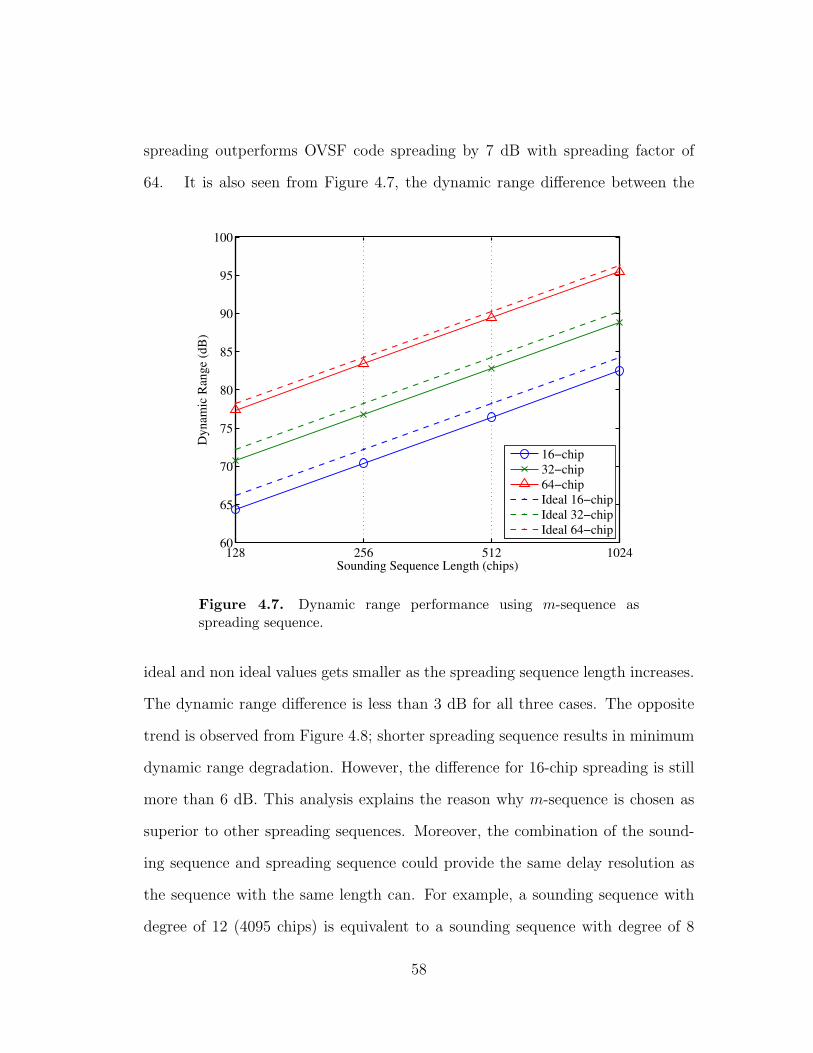
spreading outperforms OVSF code spreading by 7 dB with spreading factor of
64. It is also seen from Figure 4.7, the dynamic range difference between the
128 256 512 102460
65
70
75
80
85
90
95
100
Sounding Sequence Length (chips)
Dynam
ic R
ange
(dB
)
16−chip
32−chip
64−chip
Ideal 16−chip
Ideal 32−chip
Ideal 64−chip
Figure 4.7. Dynamic range performance using m-sequence asspreading sequence.
ideal and non ideal values gets smaller as the spreading sequence length increases.
The dynamic range difference is less than 3 dB for all three cases. The opposite
trend is observed from Figure 4.8; shorter spreading sequence results in minimum
dynamic range degradation. However, the difference for 16-chip spreading is still
more than 6 dB. This analysis explains the reason why m-sequence is chosen as
superior to other spreading sequences. Moreover, the combination of the sound-
ing sequence and spreading sequence could provide the same delay resolution as
the sequence with the same length can. For example, a sounding sequence with
degree of 12 (4095 chips) is equivalent to a sounding sequence with degree of 8
58

128 256 512 102460
65
70
75
80
85
90
95
100
Sounding Sequence Length
Dynam
ic R
ange
(dB
)
16−chip
32−chip
64−chip
Ideal 16−chip
Ideal 32−chip
Ideal 64−chip
Figure 4.8. Dynamic range performance using OVSF codes asspreading sequence.
(255 chips) spread by another sequence with degree of 4 (16 chips) in terms of
delay resolution.
There are other pseudo-random binary sequences other than the m-sequence,
such as Kasami sequences, gold sequences, Barker sequences and Williard se-
quences [69]. The choice of m-sequence is because it has the best autocorrelation
property among other PN sequences, which promises the largest dynamic range,
and periodicity. The m-sequence can be generated with a Linear Feedback Shift
Register (LFSR), which can be easily implemented on an FPGA or other pro-
grammable logic devices.
59
4.2.3 Assessing the Impact of the Proposed Channel Sounding
Technique
In addition to the performance, interference introduced by the sounding signal
to the primary and secondary users cannot be neglected. The total interference
caused by the sounding signal is evaluated by employing the primary user signal-
to-noise inteference ratio (SINR), which is defined by:
SINR (dB) = 10 log10
N∑i=1
PiIi +BN0
, (4.6)
where Pi is the transmit power for a certain primary user within the ith subcarrier
bandwidth, N0 is the noise power spectral density, and it is assumed to be the
same for all the subcarriers, Ii is the interference power introduced by the sound-
ing signal on the ith subcarrier, and N is the number of subcarriers. Since the
sounding signal is spread in the time domain, the resulting sounding signal power
becomes P(i)s − Gi, where Gi is the spreading gain for the ith subcarrier. Hence,
Equation (4.6) can be rewritten as:
SINR (dB) = 10 log10
N∑i=1
Pi
P(i)s −Gi +BiN0
, (4.7)
where Bi denotes the subcarrier bandwidth after spreading. For equal spreading
gain scenario, Gi becomes a constant, so does Bi. Equation (4.7) works for primary
users with interference tolerance greater than zero. For zero-interference tolerance,
the band is totally inaccessible when primary users are present in this band.
It is noticed that the SINR is inversely proportional to the spreading gainGi for
the ith subcarrier, increasing spreading gain will improve the SINR significantly.
60
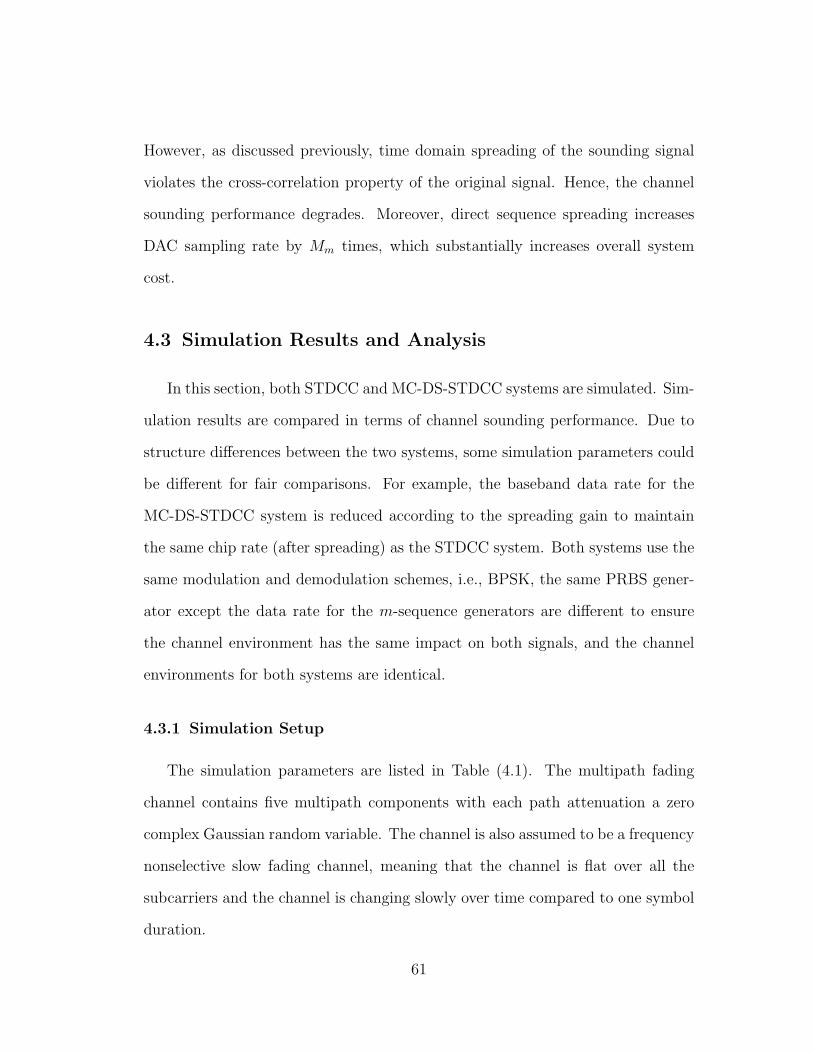
However, as discussed previously, time domain spreading of the sounding signal
violates the cross-correlation property of the original signal. Hence, the channel
sounding performance degrades. Moreover, direct sequence spreading increases
DAC sampling rate by Mm times, which substantially increases overall system
cost.
4.3 Simulation Results and Analysis
In this section, both STDCC and MC-DS-STDCC systems are simulated. Sim-
ulation results are compared in terms of channel sounding performance. Due to
structure differences between the two systems, some simulation parameters could
be different for fair comparisons. For example, the baseband data rate for the
MC-DS-STDCC system is reduced according to the spreading gain to maintain
the same chip rate (after spreading) as the STDCC system. Both systems use the
same modulation and demodulation schemes, i.e., BPSK, the same PRBS gener-
ator except the data rate for the m-sequence generators are different to ensure
the channel environment has the same impact on both signals, and the channel
environments for both systems are identical.
4.3.1 Simulation Setup
The simulation parameters are listed in Table (4.1). The multipath fading
channel contains five multipath components with each path attenuation a zero
complex Gaussian random variable. The channel is also assumed to be a frequency
nonselective slow fading channel, meaning that the channel is flat over all the
subcarriers and the channel is changing slowly over time compared to one symbol
duration.
61
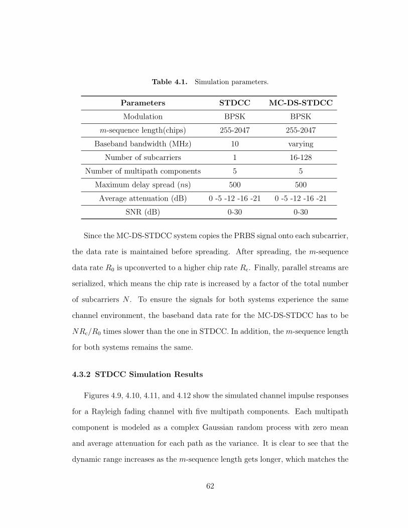
Table 4.1. Simulation parameters.
Parameters STDCC MC-DS-STDCC
Modulation BPSK BPSK
m-sequence length(chips) 255-2047 255-2047
Baseband bandwidth (MHz) 10 varying
Number of subcarriers 1 16-128
Number of multipath components 5 5
Maximum delay spread (ns) 500 500
Average attenuation (dB) 0 -5 -12 -16 -21 0 -5 -12 -16 -21
SNR (dB) 0-30 0-30
Since the MC-DS-STDCC system copies the PRBS signal onto each subcarrier,
the data rate is maintained before spreading. After spreading, the m-sequence
data rate R0 is upconverted to a higher chip rate Rc. Finally, parallel streams are
serialized, which means the chip rate is increased by a factor of the total number
of subcarriers N . To ensure the signals for both systems experience the same
channel environment, the baseband data rate for the MC-DS-STDCC has to be
NRc/R0 times slower than the one in STDCC. In addition, the m-sequence length
for both systems remains the same.
4.3.2 STDCC Simulation Results
Figures 4.9, 4.10, 4.11, and 4.12 show the simulated channel impulse responses
for a Rayleigh fading channel with five multipath components. Each multipath
component is modeled as a complex Gaussian random process with zero mean
and average attenuation for each path as the variance. It is clear to see that the
dynamic range increases as the m-sequence length gets longer, which matches the
62

0 0.2 0.4 0.6 0.8 1
x 10−6
−70
−60
−50
−40
−30
−20
−10
0
10
Delay (s)
Re
lative
Po
we
r (d
B)
Figure 4.9. Simulated channel impulse response. SNR=0 dB; pathdelay=100,190,320,430,500 ns; average attenuation=0,-5,-12,-16,-21 dB, respectively; m-sequence length = 255.
theoretical analysis. This feature is especially essential for DSA networks where
the transmit power is limited, because larger dynamic range allows weaker channel
impulse response to be detected.
It is also noticed that the dynamic range performance degrades dramatically
as the channel environment becomes complicated (e.g., multipath fading). The
ideal dynamic range can be referred to in Table 3.1. For instance, the ideal
dynamic range for an m-sequence length of 255 is 48.1 dB, but the simulation
results show that the weakest detectable signal is roughly 30 dB lower than the
strongest. In this set of simulations, the chip rate is set to 100 chips/s to ensure
that two adjacent delay paths are resolvable. As discussed in the previous chapter,
the maximum delay spread that can be measured by the system is: m/Rc, take
63

0 0.2 0.4 0.6 0.8 1
x 10−6
−70
−60
−50
−40
−30
−20
−10
0
10
Delay (s)
Re
lative
Po
we
r (d
B)
Figure 4.10. Simulated channel impulse response. SNR=0 dB; pathdelay=100,190,320,430,500 ns; average attenuation=0,-5,-12,-16,-21 dB, respectively; m-sequence length = 511.
0 0.2 0.4 0.6 0.8 1
x 10−6
−70
−60
−50
−40
−30
−20
−10
0
10
Delay (s)
Re
lative
Po
we
r (d
B)
Figure 4.11. Simulated channel impulse response. SNR=0 dB; pathdelay=100,190,320,430,500 ns; average attenuation=0,-5,-12,-16,-21 dB, respectively; m-sequence length = 1023.
64

0 0.2 0.4 0.6 0.8 1
x 10−6
−70
−60
−50
−40
−30
−20
−10
0
10
Delay (s)
Re
lative
Po
we
r (d
B)
Figure 4.12. Simulated channel impulse response. SNR=0 dB; pathdelay=100,190,320,430,500 ns; average attenuation=0,-5,-12,-16,-21 dB, respectively; m-sequence length = 2047.
m = 255 for example:
τmax =255
80 MHz= 3.1875 µs. (4.8)
In Equation (4.8), the original signal is upsampled to 80 MHz, i.e., there are eight
samples per chip instead of one sample per chip for a better resolution. The
maximum path delay set in the simulation is 0.5 µs, which means the system is
capable of measuring all the path delays.
To validate the simulation model and the causes of the dynamic range degra-
dation, the following simulations were conducted:
• AWGN channel: SNR = 0 dB, 10 dB, 30 dB, 100 dB (negligible amount of
white noise) .
65

0 0.2 0.4 0.6 0.8 1
x 10−6
−70
−60
−50
−40
−30
−20
−10
0
10
Delay (s)
Re
lative
Po
we
r (d
B)
Figure 4.13. Dynamic range degradation due to white noise withoutISI with 511-bit m-sequence. Path delay=100,190,320,430,500 ns;average attenuation=0,-5,-12,-16,-21 dB, respectively; SNR=0dB.
• Multipath channel environment: no ISI, with ISI.
In Figures 4.13, 4.14, 4.15 and 4.16, the dynamic range is directly related to
the noise power, which is represented as SNR in decibels. With a nearly perfect
channel (100 dB), the dynamic range is close to the ideal value for a 511-bit
m-sequence, which is 54.2 dB. As the SNR value decreases, the dynamic range
degrades. In this case, the channel is assumed to be no ISI, meaning that the
attenuation for each path is applied to the entire sequence for one transmission
cycle, and only the signal power is attenuated. Phase shift and frequency offset is
not considered.
Figures 4.17, 4.18, 4.19 and 4.20 demonstrate the dynamic range degradation
due to ISI. In this scenario, the dynamic range does not degrade as much as it does
for the AWGN channel since the intersymbol interference power level is dominating
66

0 0.2 0.4 0.6 0.8 1
x 10−6
−70
−60
−50
−40
−30
−20
−10
0
10
Delay (s)
Re
lative
Po
we
r (d
B)
Figure 4.14. Dynamic range degradation due to white noise withoutISI with 511-bit m-sequence. Path delay=100,190,320,430,500 ns;average attenuation=0,-5,-12,-16,-21 dB, respectively; SNR=10dB.
0 0.2 0.4 0.6 0.8 1
x 10−6
−70
−60
−50
−40
−30
−20
−10
0
10
Delay (s)
Re
lative
Po
we
r (d
B)
Figure 4.15. Dynamic range degradation due to white noise withoutISI with 511-bit m-sequence. Path delay=100,190,320,430,500 ns;average attenuation=0,-5,-12,-16,-21 dB, respectively; SNR=30dB.
67

0 0.2 0.4 0.6 0.8 1
x 10−6
−70
−60
−50
−40
−30
−20
−10
0
10
Delay (s)
Re
lative
Po
we
r (d
B)
Figure 4.16. Dynamic range degradation due to white noise withoutISI with 511-bit m-sequence. Path delay=100,190,320,430,500 ns;average attenuation=0,-5,-12,-16,-21 dB, respectively; SNR=100dB.
over the noise power. Comparing Figure 4.17 with 4.13, it is found that the ISI
introduces approximately 10 dB degradation in dynamic range. This analysis is
intuitive, although the intersymbol interference power could be quantified in terms
of frequency error [64], which will not be discussed in detail here.
68
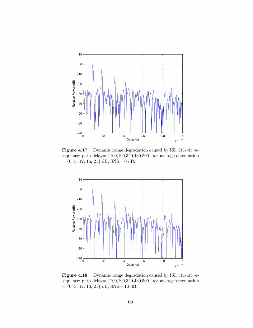
0 0.2 0.4 0.6 0.8 1
x 10−6
−70
−60
−50
−40
−30
−20
−10
0
10
Delay (s)
Re
lative
Po
we
r (d
B)
Figure 4.17. Dynamic range degradation caused by ISI. 511-bit m-sequence; path delay= 100,190,320,430,500 ns; average attenuation= 0,-5,-12,-16,-21 dB; SNR= 0 dB.
0 0.2 0.4 0.6 0.8 1
x 10−6
−70
−60
−50
−40
−30
−20
−10
0
10
Delay (s)
Re
lative
Po
we
r (d
B)
Figure 4.18. Dynamic range degradation caused by ISI. 511-bit m-sequence; path delay= 100,190,320,430,500 ns; average attenuation= 0,-5,-12,-16,-21 dB; SNR= 10 dB.
69

0 0.2 0.4 0.6 0.8 1
x 10−6
−70
−60
−50
−40
−30
−20
−10
0
10
Delay (s)
Re
lative
Po
we
r (d
B)
Figure 4.19. Dynamic range degradation caused by ISI. 511-bit m-sequence; path delay= 100,190,320,430,500 ns; average attenuation= 0,-5,-12,-16,-21 dB; SNR= 30 dB.
0 0.2 0.4 0.6 0.8 1
x 10−6
−70
−60
−50
−40
−30
−20
−10
0
10
Delay (s)
Re
lative
Po
we
r (d
B)
Figure 4.20. Dynamic range degradation caused by ISI. 511-bit m-sequence; path delay= 100,190,320,430,500 ns; average attenuation= 0,-5,-12,-16,-21 dB; SNR=100 dB.
70

−2 −1 0 1 2 3 4 5
x 107
0
0.2
0.4
0.6
0.8
1
1.2
Bandwidth (Hz).
No
rma
lize
d P
ow
er
Figure 4.21. Power spectral density of MC-DS-STDCC signal with16 subcarriers and total transmission bandwidth of 30 MHz.
4.3.3 MC-DS-STDCC Simulation Results
The simulation setup is basically the same as the STDCC system, except the
chip rate is different. It is also assumed that the channel is flat over subcarriers.
One of the advantages of MC-DS-STDCC systems, as discussed before, is the
ability to be operated at different center frequencies with various transmit powers.
An example can be seen from Figure 4.21, where the dashed line represents the
transmit power limits, and solid curves are the signal spectrum. Each curve is a
sinc(·) function. It is easy to notice that the bandwidth of each subcarrier is the
same but the power is different. In some of the Ultra-Wideband (UWB) appli-
cations, pulse shaping is used to ensure the ultra-wideband signal spectrum fits,
for instance the FCC mask [39]. The multicarrier modulation technique provides
a more adaptive way of spectrum control. In addition, digital signal processing
techniques, such as windowing and sidelobe cancellation can also be applied to
71
0 200 400 600 800 1000
−60
−40
−20
0
Delay (ns)
Re
lative
Po
we
r (d
B)
0 200 400 600 800 1000
−60
−40
−20
0
Delay (ns)
Re
lative
Po
wer
(dB
)
STDCC
SC−DS−STDCC
Figure 4.22. SC-DS-STDCC with 16-bit spreading sequence vs.STDCC. The delay of each path is 100,200,300,400,500 ns, and theaverage attenuation of each path is 0,-10,-15,-20,-25 dB, respectively.
the transmitted and received sounding signals to improve the performance as well
as to reduce the spectral efficiency [70–72].
To validate the MC-DS-STDCC simulation model, we started with a single-
carrier direct sequence STDCC (SC-DS-STDCC) system, comparing the simula-
tion result with the STDCC system. Since there is only one subcarrier in the
MC-DS-STDCC system, the copier, P/S, S/P, IFFT, and FFT can be treated
as redundant blocks, which do not change the data sequence, except spreading
and despreading. Figure 4.22 shows the estimated channel impulse response. The
performances of both SC-DS-STDCC and STDCC systems are identical, except
that the error floor of the SC-DS-STDCC is about 12 dB (10 log10(16), spreading
sequence length is 16) lower than the STDCC system. This is because of the
processing gain introduced by the time domain spreading process.
72

Figure 4.23. MC-DS-STDCC simulation results with 16 subcarriersand 511-bit m-sequence. The delay of each path is 100,190,320,430,500ns, and the average attenuation of each path is 0,-5,-12,-16,-21 dB,respectively.
Figure 4.23 shows an estimated channel impulse response of a 16-subcarrier
MC-DS-STDCC system in presence of a flat fading channel. The power is normal-
ized with respect to the first multipath component, and it is flat over subcarriers.
For the rest of the multipath components, the power level is varying over subcar-
riers, which is due to Gaussian white noise.
4.3.4 Mean Squared Error of the CIR Estimation
In this section, the MC-DS-STDCC channel sounder performance is evaluated
by introducing the mean squared error of the estimated CIRs for various cases.
73

The MSE of the estimated CIRs is defined as the following:
MSE(t) = E[(Pci (τ)− Pci (τ))2] , (4.9)
where Pci (τ) and Pci (τ) represent the the power levels associated with each chan-
nel impulse response at delay τ for the estimated CIR, and actual CIR, respec-
tively. The MSE is estimated by averaging the CIR over a time period of T . The
m-sequence length varies from 127 to 511 chips, number of subcarriers chosen are
16, 32 and 64, and the spreading sequence length for m-sequence spreading and
OVSF code spreading is 15, 16 and 31, 32, respectively. The MSE perfor-
mance is compared with different system parameter combinations.
−25 −20 −15 −10 −5 0 5 10 15 2010
−4
10−3
10−2
SNR (dB)
CIR
MS
E
L=127, N=16, Mm
=15
L=511, N=16, Mm
=15
L=127, N=32, Mm
=15
L=511, N=32, Mm
=15
L=127, N=64, Mm
=15
L=511, N=64, Mm
=15
Figure 4.24. MC-DS-STDCC MSE performance. L = 127, 511;N = 16, 32, 64; Mm=15.
Figure 4.24 compares the MSE performance between m-sequence and OVSF
code spreading with spreading sequence length of 15 and 16, respectively. The
74
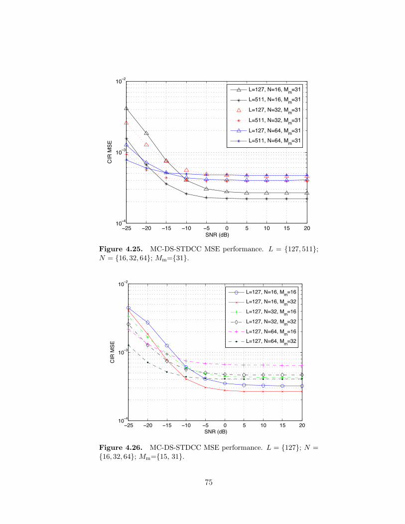
−25 −20 −15 −10 −5 0 5 10 15 2010
−4
10−3
10−2
SNR (dB)
CIR
MS
E
L=127, N=16, Mm
=31
L=511, N=16, Mm
=31
L=127, N=32, Mm
=31
L=511, N=32, Mm
=31
L=127, N=64, Mm
=31
L=511, N=64, Mm
=31
Figure 4.25. MC-DS-STDCC MSE performance. L = 127, 511;N = 16, 32, 64; Mm=31.
−25 −20 −15 −10 −5 0 5 10 15 2010
−4
10−3
10−2
SNR (dB)
CIR
MS
E
L=127, N=16, Mm
=16
L=127, N=16, Mm
=32
L=127, N=32, Mm
=16
L=127, N=32, Mm
=32
L=127, N=64, Mm
=16
L=127, N=64, Mm
=32
Figure 4.26. MC-DS-STDCC MSE performance. L = 127; N =16, 32, 64; Mm=15, 31.
75
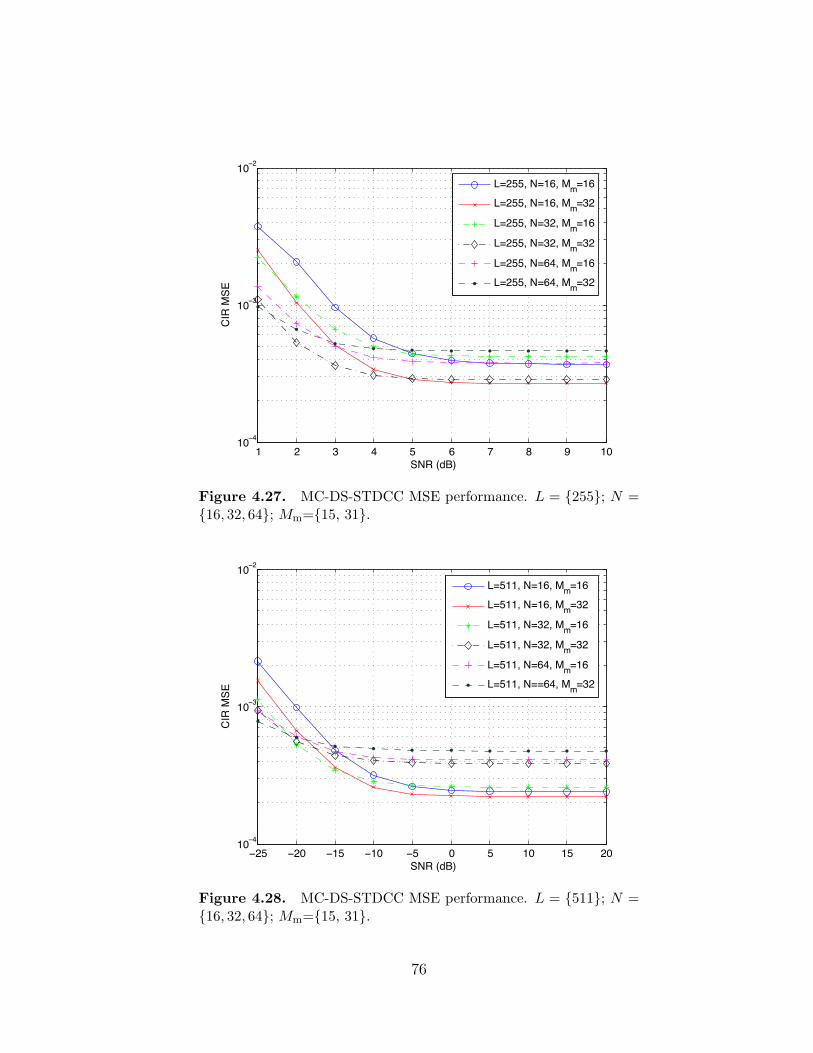
1 2 3 4 5 6 7 8 9 1010
−4
10−3
10−2
SNR (dB)
CIR
MS
E
L=255, N=16, Mm
=16
L=255, N=16, Mm
=32
L=255, N=32, Mm
=16
L=255, N=32, Mm
=32
L=255, N=64, Mm
=16
L=255, N=64, Mm
=32
Figure 4.27. MC-DS-STDCC MSE performance. L = 255; N =16, 32, 64; Mm=15, 31.
−25 −20 −15 −10 −5 0 5 10 15 2010
−4
10−3
10−2
SNR (dB)
CIR
MS
E
L=511, N=16, Mm
=16
L=511, N=16, Mm
=32
L=511, N=32, Mm
=16
L=511, N=32, Mm
=32
L=511, N=64, Mm
=16
L=511, N==64, Mm
=32
Figure 4.28. MC-DS-STDCC MSE performance. L = 511; N =16, 32, 64; Mm=15, 31.
76

sounding m-sequence length is L=127, 511, and the number of subcarriers are
16, 32 and 64. As the length of the sounding sequence increases, the MSE er-
ror floor decreases. This is because a longer m-sequence provides more inherent
processing gain. It is also noticed that 64-subcarrier case results in a worse MSE
performance than 32 and 16 subcarriers. Since increasing the number of subcar-
riers also broadens the noise bandwidth, hence the SNR decreases, which is what
causes the MSE error floor to rise.
Comparing Figure 4.25 with Figure 4.24, doubling the length of the spreading
sequence reduces the MSE error floor by approximately 6 dB for the combination
of L = 511, N = 64. In this case, 32- and 64-subcarrier systems almost perform
the same when the SNR is greater than -10 dB. 16-subcarrier system outperforms
the other two when the channel SNR value is greater than -10 dB. As discussed
previously, a larger number of subcarriers delivers a more frequency-agile channel
sounder, since the subcarrier power can be fine tuned to fit the transmit power
restriction. However, it does not perform as well as less subcarrier systems in
terms of CIR estimation accuracy due to the extra noise introduced.
Figures 4.26, 4.27 and 4.28 demonstrate the MSE performance with fixed
sounding sequence length L with various N and Mm combinations. They share
the same trend as analyzed before, that is, longer spreading sequence provides
more processing gain, and hence the MSE error floor decreases. Systems with a
larger number of subcarriers introduce wider noise bandwidth, which lower the
channel SNR, and hence the MSE performance degrades.
Observe that there appears an irreducible error floor in each figure, which is
caused by multi-carrier interference. Qinghua and Coulson have provided detailed
BER error floor analysis in [73,74] for MC-CDMA and OFDM systems. Although
77

the BER error floor analysis does not apply directly to the MSE floor, the cause
of the error floor is the same. Considering an MC-CDMA system, we define Pe as
the average error floor among all subcarriers, and it is given by [73]:
Pe =1
N
N∑i=1
Pe,i, (4.10)
where Pe,i is the unconditional error floor of the ith subcarrier, and K denotes
the total number of subcarriers. Equation (4.10) indicates that the larger the
number of subcarriers, the higher the irreducible error floor. The same conclusion
can be drawn from Figures 4.24 through 4.28. In addition to the MC-CDMA
system, direct-sequence spreading provides inherent processing gain for the MSE
performance. Assume that Gi is the spreading gain for the ith subcarrier, then
Equation (4.10) becomes:
Pe =1
N
N∑i=1
(Pe,i −Gi) . (4.11)
When N = 1, the system simplifies to a single carrier direct-sequence CDMA
system, and the error floor analysis can be found in [75].
Overall, one can change the MC-DS-STDCC channel sounder parameters de-
pending on the system requirements, channel sounding accuracy, interference level,
etc. When designing a channel sounding system for DSA networks, many factors
such as, hardware complexity, interference level, and channel sounding perfor-
mance, need to be considered. This leads to a multi-objective problem, and a
tradeoff has to be made before design.
78

4.4 Chapter Summary
In this chapter, the MC-DS-STDCC channel sounding technique was explained
in detail. System schematics and its mathematical expression of the signal were
presented. The system parameters were strengthened. In the end, the chapter
is concluded by simulation results and analysis. A sanity check of the proposed
technique was done by simulating a Single-Carrier DS-STDCC system and com-
pared with the STDCC simulation result in order to validate the simulation model.
A simple 16-subcarrier MC-DS-STDCC system was also simulated with flat fad-
ing channel. Further simulations on frequency selective and non equal subcarrier
power systems needs to be conducted. On the performance analysis, the mean
squared error metric is introduced in measuring the channel sounding performance
with various system parameter combinations. The MSE performance is evaluated
from different aspects. They are, MSE versus number of subcarriers, MSE versus
m-sequence length, and MSE versus spreading sequence length. Depending on the
channel sounding measurement requirements, the simulation results can be used
as a system design guideline.
The most important feature of the MC-DS-STDCC technique is interference
awareness. However, direct sequence spread spectrum requires large bandwidth,
which results in high sampling rate. In the next chapter, an alternative solution
that is based on the OFDM system will be discussed. This solution does not
require a high sampling rate compared to the MC-DS-STDCC technique, and
hence, the implementation is simple. Moreover, the OFDM-based sounder ex-
tracts channel information from the user transmit data such that no sounding
signal generation is required.
79

Chapter 5
OFDM-Based Channel Sounder
5.1 Ultra Wideband Channel Sounder
An ultra-wideband (UWB) channel sounder can perform channel sounding
across a very wide bandwidth of up to gigahertz. However, it has several poten-
tial problems when the FCC regulations are applied. A UWB channel sounder
generates an extremely narrow pulse (i.e., nanoseconds) in the time domain, such
as a Gaussian monocycle pulse [76], to record the reflected paths of the mo-
bile radio channel. Although a UWB sounder can achieve high multipath delay
resolution and spectrum utilization efficiency, narrow pulses suffer from the peak-
to-average power (PAPR) problem, which requires large power amplifier dynamic
range. Moreover, studies have shown that the UWB systems could cause interfer-
ence with other systems [77,78]. Hence, pulse shaping must be applied to the pulse
before being transmitted. However, to fit the transmitted signal spectrum under
the FCC mask, sophisticated pulse shaping algorithms are required. Furthermore,
when the UWB channel sounder is operated in the DSA network environment,
where primary and secondary users are sharing the spectrum resource, more re-
80

striction, such as frequency band availability, will be added in addition to the
FCC regulations, which could make pulse shaping infeasible or, at the cost of long
computation time.
5.2 OFDM Systems Overview
S/Ps[n]C
on
stel
lati
on
Map
pin
gIFFT P/S s(t)
Xk
X1
X2
X3
(a) OFDM transmitter.
S/Pr(t) FFT
Sy
mb
ol
Det
ecti
on
P/S s’[n]
Yk
Y1
Y2
Y3
(b) OFDM receiver.
Figure 5.1. OFDM transceiver architecture.
OFDM systems use the spectrum resource more efficiently by transmitting
data using orthogonal subcarriers. As shown in Figure 5.1, the serial data s [n]
stream is first converted to N parallel streams, where N is the number of sub-
carriers, each parallel data stream is modulated onto a different subcarrier. The
mathematical expression is defined as the following:
s(t) =N−1∑k=0
Xkej2πkt/T , 0 ≤ t < T, (5.1)
81

where Xk are the data symbols, T is the OFDM symbol time. The subcarrier
spacing is defined as 1/T , which makes them orthogonal over one symbol period.
The modulated parallel streams are transmitted after parallel to serial con-
version. The receiver performs the reverse operation to recover the signal. The
OFDM signal bandwidth is a function of the number of subcarriers as well as the
subcarrier bandwidth. For example, an OFDM system of 1024 subcarriers with
subcarrier bandwidth of 200 KHz will generate a total bandwidth of 200 MHz
spectrum. If a UWB system is used to generate a 200 MHz bandwidth signal, it
would require a 5 ns pulse in the time domain. The theoretical spectrum of an
OFDM system is shown in Figure 5.2(a).
OFDM is considered as one of the major candidates for the DSA technology
because of its spectrum efficiency and spectral robustness. In other words, the
OFDM system can achieve spectrum shaping by adjusting the power level of cer-
tain subcarriers. In Figure 5.2(b), the relative transmit power level of an OFDM
system is limited to 0, -20, -10, -5 dB across the restricted band respectively. To
achieve OFDM spectrum shaping, the most straightforward way is to attenuate
certain subcarrier power level. However, this approach requires prior informa-
tion of the radio channel, which is feasible for the policy-based1 DSA network.
In an environment where spectrum accessibility and transmit power are totally
determined by the user, a more agile approach is needed.
It can also be observed that the sidelobe power level exceeds the FCC limit.
However, this can reduced by applying a sidelobe cancellation algorithm [79],
which is beyond the scope of this work.
1The DSA networks are generally categorized into policy-based and nonpolicy-based, wherethe former requires full knowledge of the channel environment to function, and the latter doesnot.
82

−1 −0.5 0 0.5 1−45
−40
−35
−30
−25
−20
−15
−10
−5
0
5
10
No
rmal
ized
Po
wer
Sp
ectr
um
Den
sity
(d
B)
Normalized Frequency (×π rad/sample)
(a) Theoretical OFDM signal spectrum with 256 subcarriers.
−1 −0.5 0 0.5 1−45
−40
−35
−30
−25
−20
−15
−10
−5
0
5
10
No
rmal
ized
Po
wer
Sp
ectr
um
Den
sity
(d
B)
Normalized Frequency (×π rad/sample)
PSD of OFDM signal
FCC Mask
(b) OFDM signal spectrum with subcarrier power adjustment under the FCCmask
Figure 5.2. OFDM signal spectrum.
83
Considering the design perspective of a wideband channel sounder for the DSA
network, the spectral robustness and efficiency feature of the OFDM system can be
adapted. As mentioned in Chapter 4, the channel sounder operating in the DSA
network has to introduce minimum amount of interference to the other users while
maintaining sounding performance. Complexity in both hardware and software
design is also critical. In the following section, an OFDM-based channel sounder
will be discussed with focus on the aforementioned design considerations.
5.3 OFDM-Based Channel Sounder for Cognitive Radios
The motivation of designing an ideal channel sounder for the DSA network
environment falls back to the basic principle of channel sounding, which is theo-
retically simple and easy to achieve. Hence, the question becomes how to approach
the simple solution by not increasing the hardware complexity as well as software
processing. Given a cognitive radio transceiver, the ideal design of such a sounder
is to use the CR transceiver as a sounder, which is at no cost in terms of hardware
and software design. Generally, the CR transceiver is not designed for such a
purpose, which leads to the question of minimizing the modification of an existing
CR transceiver.
As shown previously in Figure 2.4, the radio channel characteristics are closely
related to each other. For example, the channel frequency correlation function and
the power delay profile are a Fourier Transform pair, so are the Doppler power
spectrum and the time correlation function. For the OFDM system, the baseband
signal is generally considered as a “frequency domain” signal before the IFFT and
after the FFT at the transmitter and receiver respectively. The signal is converted
back and forth between the time and frequency domains during the entire trans-
84

S/Ps[n]
Co
nst
ella
tio
n
Map
pin
g
IFFT P/S s(t)
Xk
X1
X2
X3
g1
g2
g3
gk
(a) OFDM sounder transmitter architecture.
S/Pr(t) FFT
Sy
mb
ol
Det
ecti
on
P/S s’[n]
Yk
Y1
Y2
Y3
IFFT Processing
(b) OFDM sounder receiver architecture.
Figure 5.3. OFDM-based sounder transceiver architecture.
mission and reception. This feature provides a way of obtaining the time domain
characteristic of the radio channel if the frequency domain characteristic can be
captured by the OFDM transceiver. Ideally, the channel sounding device trans-
mits an impulse to excite the radio channel, and the distorted signal is received
at the receiver so that the multipath components are resolved.
Figure 5.3 demonstrates the system architecture for the OFDM-based channel
sounder. For an OFDM transmitter, the serial data stream is converted into N
parallel substreams and passed to the OFDM modulator. OFDM modulation is
generally done by the IFFT [64], the signal before and after the IFFT is considered
as frequency domain and time domain signal, respectively. The IFFT converts a
frequency domain signal into time domain so that it can be used as the sounding
signal. Theoretically, the inverse Fourier Transform of a band unlimited constant
85
amplitude signal is a delta function (impulse), which is impossible to achieve
practically. However, a band limited signal with fairly large bandwidth in the
frequency domain will provide a narrow pulse in the time domain. For example,
a rectangular window with bandwidth of 100 MHz in the frequency domain is
equivalent to a 10 ns pulse in the time domain. If this narrow pulse is transmitted
over a multipath channel, it will provide a delay resolution of 10 ns. On each
subcarrier, the power level is controlled by a tunable gain gi before the signal is
serialized and transmitted. The advantage of using tunable gain to adjust the
power level of each subcarrier is simplicity compared to spreading for the MC-
DS-STDCC system. However, a small power level will result in a CIR estimation
degradation for the OFDM-based sounder.
At the receiver, the received signal is again converted into N substreams and
demodulated with FFT, which transforms the time domain signal into frequency
domain. The output of the FFT block is an estimation of the frequency correlation
function. The time domain characteristics of the radio channel can be obtained by
transforming the the output signal of the FFT block into the time domain using
inverse Fourier Transform and time shifting.
Comparing Figures 5.1 and 5.3, the only addition to the OFDM transmitter
is the tunable gain. On the receive side, the output of the FFT block is first
extracted and stored on the computer, both the IFFT and postprocessing can
be done off-line. Furthermore, the MC-DS-STDCC receiver also requires knowl-
edge of the spreading sequence length used on each subcarrier in order to perform
despreading, while the OFDM-based channel sounder does not perform such in-
formation exchange between the transmitter and the receiver.
86

5.3.1 System Parameters
In general, the OFDM-based channel sounding system parameters are mini-
mum delay resolution, maximum detectable delay, dynamic range and processing
time.
• Delay Resolution ∆τ .
Similar to the conventional channel sounding systems, the minimum delay
resolution is determined by the baseband sampling rate of the system. In
this case, since the sounding signal is one OFDM symbol, the minimum delay
resolution is equal to the inverse of the OFDM system baseband bandwidth,
that is:
∆τ =1
Bs
. (5.2)
• Maximum Detectable Delay τmax.
The maximum detectable delay is equivalent to one OFDM symbol period
Ts. In a time-variant channel, where channel condition changes frequently,
channel sounding has to be performed frequently in order to keep the channel
information up-to-date.
• Dynamic Range D.
Channel sounding performance is mainly affected by the dynamic range,
the larger the dynamic range, lower the threshold can be set. The dynamic
range of a sliding correlator based channel sounder is proportional to the
m-sequence length, where the dynamic range is determined by the DFT size
N for the OFDM-based channel sounder. The Discrete Fourier Transform
87
(DFT) is defined as:
Xk =N−1∑n=0
xne−2πiN
nk, k = 0, . . . , N − 1, (5.3)
where xn is the time domain discrete signal. If xn = 1, ∀n, the amplitude
of Xk = N . Hence, the dynamic range in decibels is calculated as:
DdB = 10 log10N. (5.4)
Note that the contribution to the dynamic range only comes from the non-
zero data points, if the sounding signal contains zeros, the dynamic range
will be degraded, and hence Equation (5.4) becomes:
D′dB = 10 log10N′. (5.5)
More details on sounding singal design will be discussed in the following
section.
• Processing Time.
The processing time defines how long it takes for the system to complete
the channel impulse response computation. Sliding correlator based channel
sounder’s processing time is a function of the m-sequence length M and the
chip rate Rc. For example, a 4095-chip (212 − 1) m-sequence at chip rate of
32 Mcps needs 4095× 4095/32e6 ≈ 0.5 (s) to compute the channel impulse
response across all phases of the entire m-sequence. Since the OFDM-based
channel sounder does not require cross-correlation process at the receiver,
the processing time is determined by the FFT algorithm. It is known that
88

the FFT reduces the number of operations from O (N2) for the DFT to
O (N logN). For example, the USRP uses Altera CycloneTMFPGA. If the
FPGA is running at 250 MHz, the processing time for a 4096-point DFT
is equal to 40962/250e6 ≈ 0.067 (s), which is significantly shorter than the
sliding correlator based channel sounder.
5.4 Sounding Signal and Performance
As discussed in the previous section, in order to design a suboptimal sounding
signal, one has to transmit a constant envelop signal across one OFDM symbol,
which is an ideal scenario for a unlicensed user. However, this approach is subject
to subband availability and signal power level restrictions. Furthermore, dedicat-
ing transmission slots to the sounding signal reduces the user overall throughput
and also increases the PAPR for the system. Our research shows that one can use
the user data as the sounding signal to minimize the system overhead. Given a
fixed bandwidth, the channel sounding accuracy, in terms of MSE, is a function
of the number of subcarriers as well as the correlation factor of the user transmit
data. In this section, the impact on the channel sounding accuracy caused by
impairment of the sounding signal and using user data as sounding signal will be
discussed, and a tradeoff study is conducted to identify the confidence of channel
sounding accuracy.
5.4.1 Guaranteed Spectrum Availability
The channel sounding accuracy is limited by the signal transmit power or
signal-to-noise (SNR) ratio when the spectrum availability is guaranteed. STDCC
and MC-DS-STDCC channel sounder are promised to work under a low SNR
89

condition because of the inherent processing gain provided by the cross correlation
and direct sequence spreading respectively. For the OFDM-based channel sounder,
the signal reception only depends on the radio channel SNR.2
Transmitting a highly correlated sequence (i.e., N “1” s) increases the OFDM
system peak-to-average power ratio [80]. This problem is more severe when fre-
quent channel sounding is required. However, this approach gives the best perfor-
mance in terms of sounding accuracy, and will be used as the baseline performance
for comparison purposes. This drawback leads to a demand for another channel
sounding signal design.
The properties of Fourier Transform as well as the resulting functions of certain
time domain signals provide the solution. As mentioned previously, the FT of an
infinite number of ones is an impulse in the frequency domain with zero width
and infinite amount of energy. In practice, the energy can also be stored within
a fairly short bandwidth if the time domain signal is long enough, which leads
to a optimal sounding signal. Given certain number of subcarriers, N , the more
number of ones transformed, the better the sounding signal and vice versa. On
the other hand, if a certain OFDM symbol contains zeros, the magnitude of the
resulting OFDM modulator output is a sinc-like function. Note that the definition
of DFT is [64]:
Xk =N−1∑n=0
xne−2πjN
kn, k = 0, . . . , N − 1. (5.6)
For a rectangular function xn with total number of sample M ≤ N , and assuming
2In general, the signal quality is also affected by the interference. For simplicity, it is assumethat the sounding signal is not interfered with by other signals.
90

that M is odd:
xn =
1, |n| ≤ M − 1
2
0, otherwise,
the Fourier Transform Xk is:
Xk =N−1∑n=0
xne−2πjN
kn
=sin (ωM/2)
M sin (ω/2)
≈ sin (πfM)
πf,
where ω = 2πk/N and f = k/N . From the equation above, the sinc(·) function
mainlobe width is 2 · 2π/M radian, which is inversely proportional to the time
domain number of samples M . We can define the sidelobe width ΩM , 2π/M , as
M gets larger, the mainlobe width narrows, which improves the frequency resolu-
tion. However, the window size M has no effect on sidelobe level, it only changes
the location of the zero-crossing points. The sidelobe height is instead a result of
the abruptness of the window’s transition from 1 to 0 in the time domain. This is
the same thing as the so-called Gibbs phenomenon [64] seen in truncated Fourier
series expansions of periodic waveforms. The mainlobe magnitude is always ap-
proximately 13 dB higher than the first sidelobe magnitude. The peak magnitude
difference between the mainlobe and the first side lobe determines the dynamic
range when channel sounding is performed with this signal. Hence the dynamic
range for such a signal is 13 dB. However, the dynamic range can be improved
by applying different window functions. The choice of window functions depends
91

on the system requirement such as channel SNR, channel sounding accuracy, etc.
Another method for improving the dynamic range is pulse shaping. Pulse shaping
is usually done by applying a raised-cosine filter on the input signal to reduce
spectral leakage of the signal. Figure 5.4 compares the impulse response of a
raised-cosine filter with different roll-off factors. The impulse response is a time
domain parameter, but we desire a frequency response that is sinc function like.
Since FFT and IFFT operations are reversible, the transforms themselves are
identical except one is the time-shifted version of another, so the characteristics
discussed here in one domain can also be projected to another. As can be seen,
the sidelobe peak level decreases with the increase of the roll-off factor.
Another system parameter is the delay resolution. As discussed previously,
the mainlobe width of the sinc function is equal to 2ΩM radian. For an N -point
0 5 10 15 20 25 30 35−0.4
−0.2
0
0.2
0.4
0.6
0.8
1
Sample Index
Am
pli
tud
e
r = 0
r = 0.4
r = 0.8
r = 1.0
Figure 5.4. Impulse responses of a raised-cosine filter with roll-offfactors of 0, 0.4, 0.8, 1.
92

FFT with input chip rate of Rc, the delay resolution ∆τ is defined as:
∆τ =2π
M· NRc
. (5.7)
For example, considering a time domain signal with a sampling rate of 32 Mcps,
FFT size of 1024, and windows size M = 512, the minimum delay resolution is
calculated as follows:
∆τ =2π
M· NRc
≈ 6.28× 1024
512× 32e6
≈ 39 µs.
Equation (5.7) contains a fraction N/M , and minNM = 1. This indicates that
the minimum delay resolution is only achieved when the fraction is equal to one.
When the window size is equal to N , the window function is sampled at exactly
all of it’s zero-crossings, which gives the impression of an infinitely long sinusoidal
sequence, hence the delay resolution is reduced to 2π/Rc.
5.4.2 Non-Contiguous Band
A non-contiguous band generally refers to the subbands that do not share
common borders. In other words, the target frequency band is divided into con-
tiguous subbands due to frequency availability, transmit power restrictions, and
spectrum owner restrictions. An illustration of a non-contiguous band is shown
in Figure 5.5. For example, the measurement show that there is a strong signal
appears between 400 MHz and 500 MHz band. If this band is to be used for chan-
93

nel sounding, the sounding signal has to avoid the frequency where the primary
user appears. Non-contiguous bands introduce a new challenge for the sounding
signal design, since the channel sounding needs to be done accurately as well as
“quietly.” As described previously, if the user data can be used as the sounding
signal, no additional interference will be introduced to other users. Moreover,
channel sounding can be performed more frequently (per OFDM signal period).
5.4.3 Sounding Signal Performance Analysis and Simulation Results
Based on Fourier Transform theory, if a given signal x(t) = x(t+T ) is periodic
(temporal period T ), its spectrum X[n] is discrete (Fourier series with interval
ω0 = 2π/T ). If a given signal x[m] is discrete (with temporal interval t0 between
0 0.1 0.2 0.3 0.4 0.5 0.6 0.7 0.8 0.9 1-100
-90
-80
-70
-60
-50
-40
-30
-20
-10
Frequency (GHz)
Pow
er (
dB
m)
White Space
Occupied
Figure 5.5. Spectrum occupancy measurements from 9 kHz to 1GHz (8/31/2005, Lawrence, KS, USA).
94
samples), its spectrum X(f) is periodic (frequency period Ω = 2π/t0). If a given
signal is both periodic and discrete, its spectrum is periodic and discrete. In this
case, the user data is used as the sounding signal, which is discrete but aperiodic,
and we define ρ to be the percentage of “0”s in one OFDM symbol period, that
is:
ρ =N ′
N. (5.8)
In order to investigate how channel sounding accuracy reacts when ρ changes, we
define the Mean Squared Error (MSE) of the estimated channel impulse response
as:
MSE(t) = E[(Pci (τ)− Pci (τ))2] , (5.9)
where Pci (τ) and Pci (τ) are the estimated and actual power of the channel impulse
responses respectively. In Equation (5.9), (Pci (τ)−Pci (τ)) is defined as residual,
or estimated error εi, which is the difference between the observed data and fitted
model. In an ideal case, where the estimated error is only caused by the channel
noise, the MSE is a function of the channel SNR and the dynamic range. Assuming
BPSK modulation, εi can be represented by the complementary error function:
εi =1
2erfc
(√EbN0
), (5.10)
and hence, Equation (5.9) can be rewritten as:
MSE = −(DR + SNR). (5.11)
For a multipath fading channel, both power attenuation and multipath delay
distribution will affect the accuracy of the CIR estimation. Furthermore, the
95
error estimation accuracy also depends on how the threshold is chosen. Higher
threshold will limit the amount of noise during the estimation process. However,
the multipath component with weak signal strength might be left out, which
degrades the accuracy. Assume that all the multipath components can be resolved
for a given threshold R, and the envelop of the channel impulse response has a
Rayleigh probability density function:
fR(r) =r
σ2e−r
2/(2σ2), (5.12)
where σ2 denotes the time-average power of the received signal. The probabil-
ity that the received signal does not exceed a specified value R is given by the
corresponding cumulative distribution function (CDF) [45]:
P (R) = Pr(r ≤ R) =
∫ R
0
p(r)dr = 1− e−R2/(2σ2). (5.13)
Let γ be the average Eb/N0 for a Rayleigh fading channel, and γ is defined as [81]:
γ =EbN0
[a2 + 2σ2
], (5.14)
where a2 + 2σ2 is the average power of the signal envelop. Based on Equa-
tion (5.14), the MSE for a Rayleigh fading channel is given by:
MSE = −(DR + γ). (5.15)
Figures 5.6 and 5.7 show a set of snapshots of the estimated channel impulse
responses versus the actual channel impulse responses generated by the simula-
96
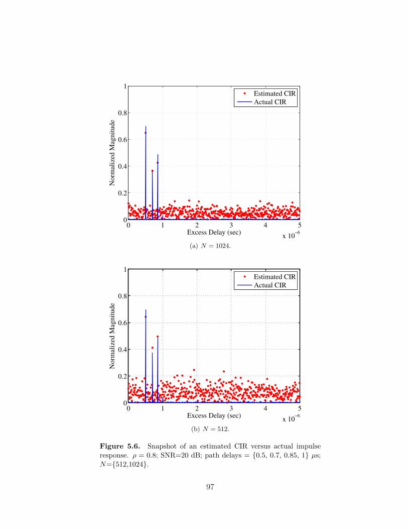
0 1 2 3 4 5
x 10−6
0
0.2
0.4
0.6
0.8
1
Excess Delay (sec)
No
rmal
ized
Mag
nit
ud
e
Estimated CIR
Actual CIR
(a) N = 1024.
0 1 2 3 4 5
x 10−6
0
0.2
0.4
0.6
0.8
1
Excess Delay (sec)
No
rmal
ized
Mag
nit
ud
e
Estimated CIR
Actual CIR
(b) N = 512.
Figure 5.6. Snapshot of an estimated CIR versus actual impulseresponse. ρ = 0.8; SNR=20 dB; path delays = 0.5, 0.7, 0.85, 1 µs;N=512,1024.
97

0 0.5 1 1.5 2 2.5 3
x 10−6
0
0.2
0.4
0.6
0.8
1
Excess Delay (sec)
No
rmai
lize
d M
agn
itu
de
Estimated CIR
Actual CIR
(a) N = 256.
0 0.2 0.4 0.6 0.8 1 1.2 1.4
x 10−6
0
0.2
0.4
0.6
0.8
1
Excess Delay (sec)
No
rmal
ized
Mag
nit
ud
e
Estimated CIR
Actual CIR
(b) N = 128.
Figure 5.7. Snapshot of an estimated CIR versus actual impulseresponse. ρ = 0.8; SNR=20 dB; path delays = 0.5, 0.7, 0.85, 1 µs;N=128,256.
98
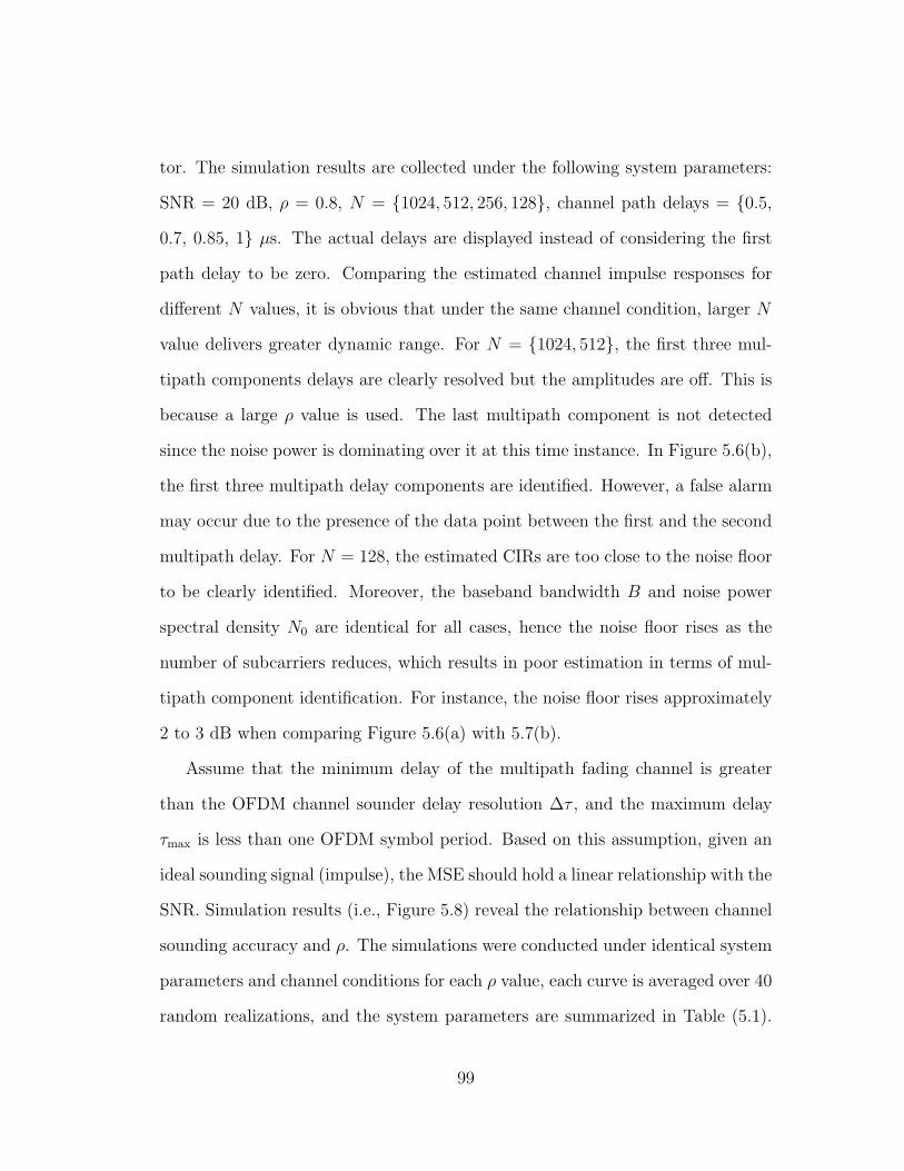
tor. The simulation results are collected under the following system parameters:
SNR = 20 dB, ρ = 0.8, N = 1024, 512, 256, 128, channel path delays = 0.5,
0.7, 0.85, 1 µs. The actual delays are displayed instead of considering the first
path delay to be zero. Comparing the estimated channel impulse responses for
different N values, it is obvious that under the same channel condition, larger N
value delivers greater dynamic range. For N = 1024, 512, the first three mul-
tipath components delays are clearly resolved but the amplitudes are off. This is
because a large ρ value is used. The last multipath component is not detected
since the noise power is dominating over it at this time instance. In Figure 5.6(b),
the first three multipath delay components are identified. However, a false alarm
may occur due to the presence of the data point between the first and the second
multipath delay. For N = 128, the estimated CIRs are too close to the noise floor
to be clearly identified. Moreover, the baseband bandwidth B and noise power
spectral density N0 are identical for all cases, hence the noise floor rises as the
number of subcarriers reduces, which results in poor estimation in terms of mul-
tipath component identification. For instance, the noise floor rises approximately
2 to 3 dB when comparing Figure 5.6(a) with 5.7(b).
Assume that the minimum delay of the multipath fading channel is greater
than the OFDM channel sounder delay resolution ∆τ , and the maximum delay
τmax is less than one OFDM symbol period. Based on this assumption, given an
ideal sounding signal (impulse), the MSE should hold a linear relationship with the
SNR. Simulation results (i.e., Figure 5.8) reveal the relationship between channel
sounding accuracy and ρ. The simulations were conducted under identical system
parameters and channel conditions for each ρ value, each curve is averaged over 40
random realizations, and the system parameters are summarized in Table (5.1).
99

Table 5.1. OFDM sounder simulation parameters.
Chip rate (Rc) 100 Mcps
Number of subcarriers (N) 1024
Channel type Rayleigh fading channel
Maximum Doppler shift 100 Hz
Multipath delays 0, 100, 200, 400 ns
Average attenuation (dB) 0, −3, −8, −12 dB
SNR (dB) −10 to 20 dB
ρ 0, 0.2, 0.4, 0.6, 0.8
As shown in the figure, the MSE performance decreases as ρ increases for almost
the entire SNR range. At small SNR values (−10 to −5 dB), the noise power
is dominating, the curves are close to each other. As SNR increases, the MSE
curves start to split. It is noticed that when ρ is equal to 0, the MSE performance
improves linearly as SNR(dB) increases, which matches the analysis.
The same trends can be observed from Figures 5.9, 5.10, and 5.11. The MSE
curves reach a certain error floor for all ρ values except for ρ = 0, and the error
floor increases as N decreases. This is because the dynamic range reduces as the
number of subcarriers gets smaller.
Figure 5.12 compares the theoretical MSE with the simulation results for dif-
ferent N values. It is clearly seen that all four curves are almost parallel to each
other, which proves the fact that the MSE performance degrades as the num-
ber of subcarriers decreases for a given SNR value (i.e., Figures 5.6 and 5.7).
For SNR equal to 10 dB, the MSEs for N = 128, 1024 are −28.93 dB and
−40.01 dB, respectively, and the difference is approximately 11 dB. Analytically,
the performance degradation caused by the dynamic range reduction is equal to
100

−10 −5 0 5 10 15 20−50
−40
−30
−20
−10
0
SNR (dB)
MS
E (
dB
)
ρ=0
ρ=0.2
ρ=0.4
ρ=0.6
ρ=0.8
Figure 5.8. OFDM sounder Mean Squared Error (MSE) perfor-mance. N = 1024, ρ = 0, 0.2, 0.4, 0.6, 0.8.
−10 −5 0 5 10 15 20−50
−40
−30
−20
−10
0
SNR (dB)
MS
E (
dB
)
ρ=0
ρ=0.2
ρ=0.4
ρ=0.6
ρ=0.8
Figure 5.9. OFDM sounder Mean Squared Error (MSE) perfor-mance. N = 512, ρ = 0, 0.2, 0.4, 0.6, 0.8.
101

−10 −5 0 5 10 15 20−50
−40
−30
−20
−10
0
SNR (dB)
MS
E (
dB
)
ρ=0
ρ=0.2
ρ=0.4
ρ=0.6
ρ=0.8
Figure 5.10. OFDM sounder Mean Squared Error (MSE) perfor-mance. N = 256, ρ = 0, 0.2, 0.4, 0.6, 0.8.
−10 −5 0 5 10 15 20−50
−40
−30
−20
−10
0
SNR (dB)
MS
E (
dB
)
ρ=0
ρ=0.2
ρ=0.4
ρ=0.6
ρ=0.8
Figure 5.11. OFDM sounder Mean Squared Error (MSE) perfor-mance. N = 128, ρ = 0, 0.2, 0.4, 0.6, 0.8.
102

−10 −5 0 5 10 15 20
−50
−40
−30
−20
−10
0
SNR (dB)
MS
E (
dB
)
N=128
N=256
N=512
N=1024
Ideal N=128
Ideal N=256
Ideal N=512
Ideal N=1024
Figure 5.12. OFDM sounder Mean Squared Error (MSE) perfor-mance. N = 128, 256, 512, 1024, ρ = 0.
10 log10(1024)− 10 log10(128) ≈ 9 dB. The 2 dB difference is caused by the noise
floor raise for different N values as discussed previously. Figure 5.12 is a better
demonstration of the linear relationship between the MSE of the estimated CIR
and the signal-to-noise ratio. The MSE for N = 1024 is observed to be −20 dB at
SNR of −10 dB, which decreases to roughly −50 dB when the SNR increases to
20 dB. Note that with larger N values, e.g., N = 1024, the simulation results are
almost identical to the theoretical results. This is because larger N value provides
better delay resolution than smaller N values, and hence, the error is primarily
caused by the noise.
103
5.5 Chapter Summary
In this chapter, a novel channel sounding technique based on OFDM transceiver
architecture is presented. The proposed OFDM channel sounder is specifically
designed for cognitive radios and dynamic spectrum access network environment.
The OFDM channel sounder achieves interference awareness by taking advantage
of the multicarrier modulation techniques. It utilizes user transmission data as
the sounding signal, hence, no extra interference is introduced to other users by
performing channel sounding. Furthermore, a signal processing algorithm that ex-
tracts the multipath channel characteristics is developed. This algorithm’s target
is minimizing system complexity as well as maintaining channel sounding per-
formance. Channel sounding performance is studied analytically, and simulation
results are provided in supporting the analysis. The proposed technique is also
evaluated for the future use in different channel environments. A tradeoff study be-
tween channel sounding performance and system complexity is conducted, which
can be used as system design guideline.
104
Chapter 6
Implementation of STDCC
Channel Sounder
In this section, several implementation issues will be discussed in detail. Both
the STDCC and the OFDM-based channel sounder implementations were exe-
cuted on the Universal Software Radio Peripheral (USRP) [12] hardware platform.
The signal processing and postprocessing functionality blocks are implemented in
the GNU Radio [82] software, an open source software radio.
6.1 USRP Hardware Prototyping Platform
The USRP, shown in Figure 6.1, is developed by Ettus Research LLC. It
allows us to create a software radio using any computer with USB 2.0 and Gigabit
ethernet ports. The operation center frequency can be changed by switching
different daughter boards, in our case, the RFX 2400 daughter board is used.
This daughter board offers a center frequency range from 2.3 GHz to 2.9 GHz
with maximum output power of 50 mW (17 dBm). The USRP mother board
105
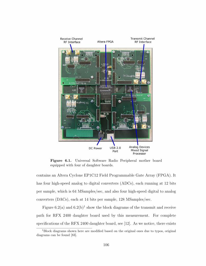
Figure 6.1. Universal Software Radio Peripheral mother boardequipped with four of daughter boards.
contains an Altera Cyclone EP1C12 Field Programmable Gate Array (FPGA). It
has four high-speed analog to digital converters (ADCs), each running at 12 bits
per sample, which is 64 MSamples/sec, and also four high-speed digital to analog
converters (DACs), each at 14 bits per sample, 128 MSamples/sec.
Figure 6.2(a) and 6.2(b)1 show the block diagrams of the transmit and receive
path for RFX 2400 daughter board used by this measurement. For complete
specifications of the RFX 2400 daughter board, see [12]. As we notice, there exists
1Block diagrams shown here are modified based on the original ones due to typos, originaldiagrams can be found [83].
106

SAWTEK855912.4 – 2.4835 GHz
FilterG6 = -2.75 dB
Tx VCOADF4360Tx PLL
AD8349-MIXQuad Mod
G2 = variable
AD9852DAC
G1 = variable
From FPGA
MGA825632LNA
G3 = 12.5 dB
RF3315LNA
G4 = 12 dB
HMC174MS8Switch
G5 = -0.6 dB
CableG7 = -L1
Antenna
To Rx SwitchDuring Receive
Transceiver Portion Common to Tx and Rx
(a) RFX2400 Transmit path.
CableG1 = -L1NF = L1
Antenna Tx/RxFrom Tx
Rx2
SAWTEK855912.4 – 2.4835 GHz
FilterG2 = -2.75 dBN2 = 2.75 dB
HMC174MS8Switch
G3 = -0.6 dBN3 = 0.6 dB
HMC174MS8Switch
G3 = -0.6 dBN4 = 0.6 dB
CableG1 = -L1NF = L1
MGA825632LNA
G5 = 12.5 dBN5 = 2.2 dB
AD8347-MIXQuad DemodG6 = 39 dB
N5 = 11.75 dB
Rx VCO
ADF4360Rx PLL
20 MHzFilter
G7 = -6 dBN7 = 6 dB
AD8347-OUTG8 = ?N8 = ?
AD9852ADC
G9 = ?N9 = ?
To FPGA
(b) RFX2400 Receive path.
Figure 6.2. RFX2400 daughter board transceiver signal flow dia-gram.
107
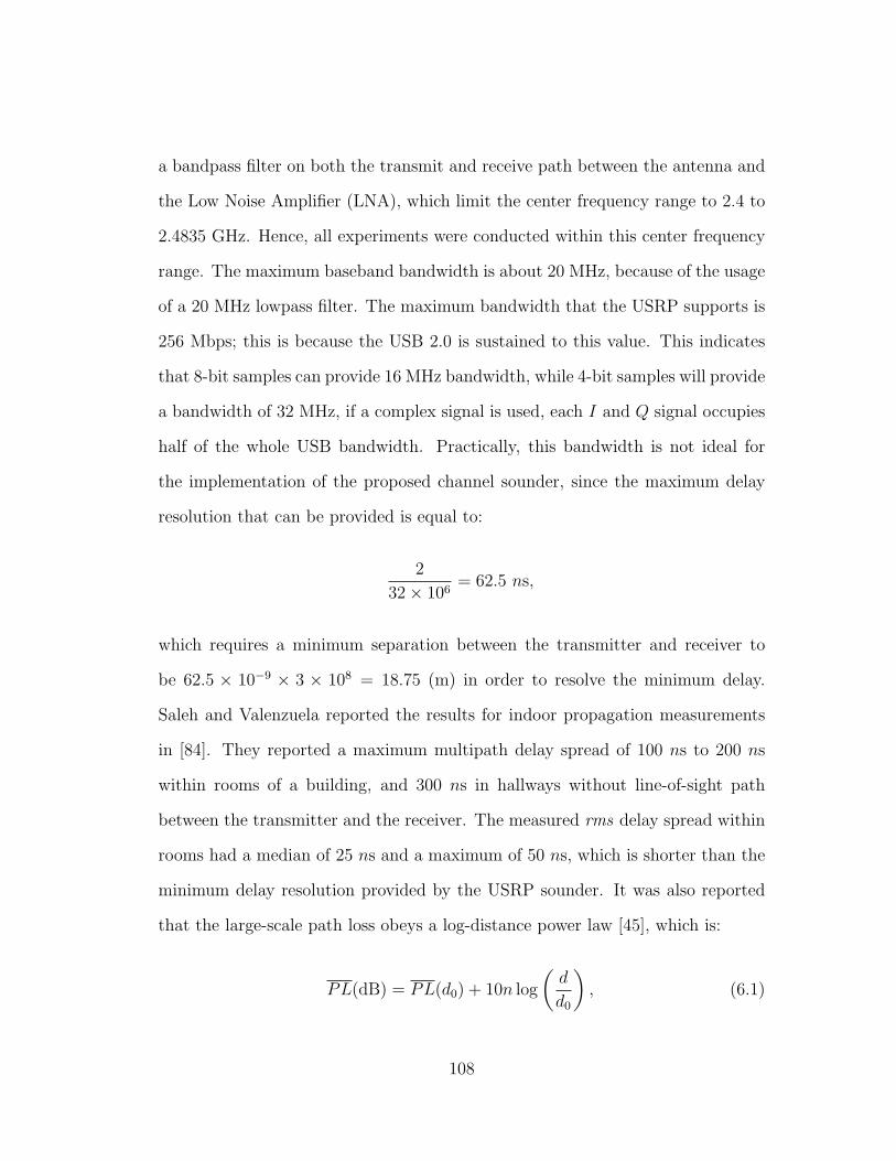
a bandpass filter on both the transmit and receive path between the antenna and
the Low Noise Amplifier (LNA), which limit the center frequency range to 2.4 to
2.4835 GHz. Hence, all experiments were conducted within this center frequency
range. The maximum baseband bandwidth is about 20 MHz, because of the usage
of a 20 MHz lowpass filter. The maximum bandwidth that the USRP supports is
256 Mbps; this is because the USB 2.0 is sustained to this value. This indicates
that 8-bit samples can provide 16 MHz bandwidth, while 4-bit samples will provide
a bandwidth of 32 MHz, if a complex signal is used, each I and Q signal occupies
half of the whole USB bandwidth. Practically, this bandwidth is not ideal for
the implementation of the proposed channel sounder, since the maximum delay
resolution that can be provided is equal to:
2
32× 106= 62.5 ns,
which requires a minimum separation between the transmitter and receiver to
be 62.5 × 10−9 × 3 × 108 = 18.75 (m) in order to resolve the minimum delay.
Saleh and Valenzuela reported the results for indoor propagation measurements
in [84]. They reported a maximum multipath delay spread of 100 ns to 200 ns
within rooms of a building, and 300 ns in hallways without line-of-sight path
between the transmitter and the receiver. The measured rms delay spread within
rooms had a median of 25 ns and a maximum of 50 ns, which is shorter than the
minimum delay resolution provided by the USRP sounder. It was also reported
that the large-scale path loss obeys a log-distance power law [45], which is:
PL(dB) = PL(d0) + 10n log
(d
d0
), (6.1)
108
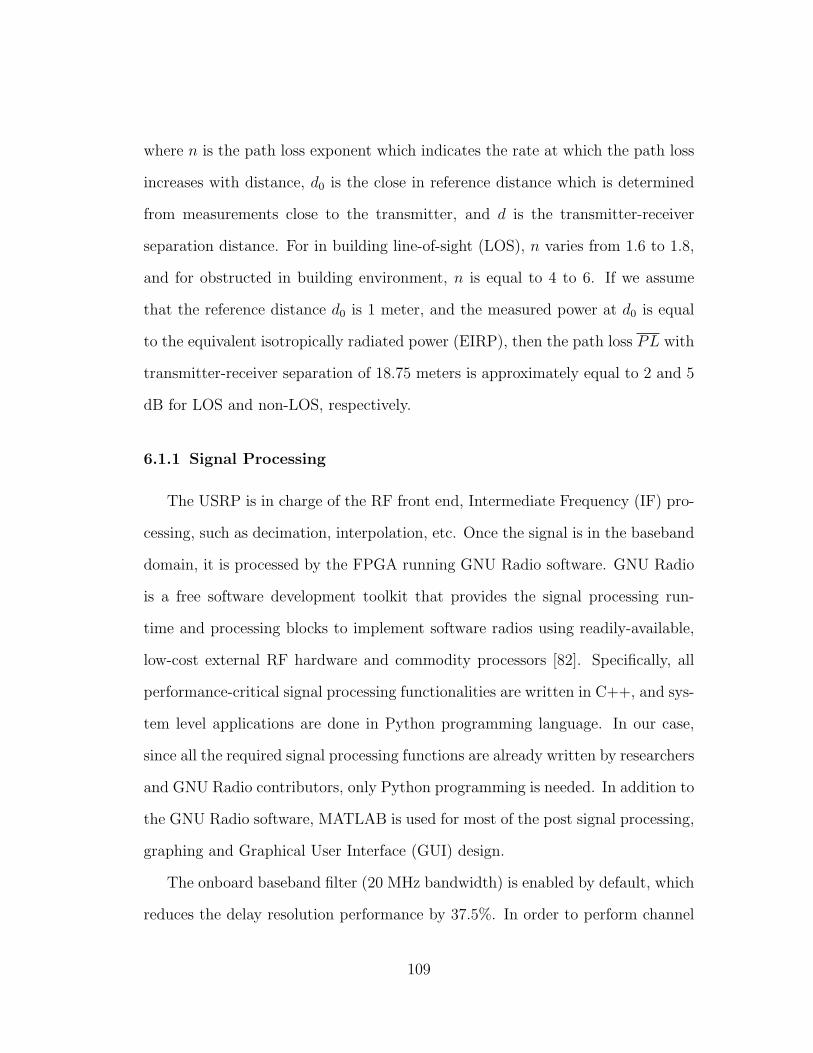
where n is the path loss exponent which indicates the rate at which the path loss
increases with distance, d0 is the close in reference distance which is determined
from measurements close to the transmitter, and d is the transmitter-receiver
separation distance. For in building line-of-sight (LOS), n varies from 1.6 to 1.8,
and for obstructed in building environment, n is equal to 4 to 6. If we assume
that the reference distance d0 is 1 meter, and the measured power at d0 is equal
to the equivalent isotropically radiated power (EIRP), then the path loss PL with
transmitter-receiver separation of 18.75 meters is approximately equal to 2 and 5
dB for LOS and non-LOS, respectively.
6.1.1 Signal Processing
The USRP is in charge of the RF front end, Intermediate Frequency (IF) pro-
cessing, such as decimation, interpolation, etc. Once the signal is in the baseband
domain, it is processed by the FPGA running GNU Radio software. GNU Radio
is a free software development toolkit that provides the signal processing run-
time and processing blocks to implement software radios using readily-available,
low-cost external RF hardware and commodity processors [82]. Specifically, all
performance-critical signal processing functionalities are written in C++, and sys-
tem level applications are done in Python programming language. In our case,
since all the required signal processing functions are already written by researchers
and GNU Radio contributors, only Python programming is needed. In addition to
the GNU Radio software, MATLAB is used for most of the post signal processing,
graphing and Graphical User Interface (GUI) design.
The onboard baseband filter (20 MHz bandwidth) is enabled by default, which
reduces the delay resolution performance by 37.5%. In order to perform channel
109

sounding measurement across the entire 32 MHz bandwidth, researchers have
developed a custom FPGA bitstream that is able to generate and receive a sounder
waveform across a full 32 MHz wide bandwidth. The waveform generation and
impulse response processing occur in logic in the USRP FPGA and not in the
host PC. This avoids the USB throughput bottleneck entirely as well as bypassing
the baseband filter. However, the OFDM-based channel sounder implementation
does not have the ability to bypass the USB throughput bottleneck. Hence, the
maximum bandwidth is limited to 20 MHz instead of 32 MHz.
6.2 Implementations of STDCC
In this section, the details of the implementations of the STDCC will be pre-
sented and experiment results will be analyzed. As discussed in Chapter 4, the
MC-DS-STDCC channel sounder requires a much higher sampling rate than what
the USRP can offer. Hence, the implementation becomes infeasible on the USRP
hardware platform. Moreover, the USRP transmitter and receiver clock synchro-
nization are not implemented by the designer of the USRP, which results in a ran-
dom time shift when the received m-sequence is cross-correlated with the locally
generated m-sequence. This issue causes inaccurate absolute multipath delays,
but relative delay estimations are still valid as far as the channel impulse response
is concerned. If we can assume that the first multipath component always con-
tains the most power, one can time shift the correlated sequence to reserve a zero
lag for the first multipath component.
Since we discovered that the clock synchronization may affect the sounding
results, we need to validate that the sounding sequences are transmitted contin-
uously without any unwanted bits between the sequences. To do this, we con-
110
0 0.2 0.4 0.6 0.8 1
x 10−3
0
2000
4000
6000
8000
10000
X: 0.0002799
Y: 8190
Delay (sec)
Mag
nit
ud
e
X: 0.0004079
Y: 8190
Figure 6.3. Channel impulse responses of a loopback test with 4095-chip m-sequence.
ducted two simple loopback tests. The first loopback test was conducted within
one USRP, an m-sequence is transmitted and routed back directly without going
through any other function blocks, then the loopback sequence is cross-correlated
with itself (autocorrelation). Intuitively, the resulting cross-correlation function
should contain a set of impulses with separation of 2m − 1 chips, where m is the
degree of the m-sequence. Figure 6.3 shows an output of the cross-correlator with
7 cycles. Each m-sequence occupies approximately 128 µs. As can be seen from
the data tips in the figure, the delay between the second and the third impulse is
exactly 128 µs. This test verifies that the same m-sequence is transmitted con-
tinuously over time. However, the appearance of the first impulse is random as
discussed previously. This test also validates that the buffer is long enough to
handle the entire process.
111

0 0.5 1 1.5 2
x 10−3
0
5
10
15
20
25
30
Delay (sec)
Mag
nit
ud
e
5.5 6 6.5
x 10−4
24
26
28
Delay (sec)
1023chips
Figure 6.4. Estimated channel impulse responses between two US-RPs with 1023-chip m-sequence.
The second test was conducted between two USRP boards, the daughter
boards used were BasicTX and RX for the purpose of simplicity and avoiding
unnecessary interference. For this test, two daughter board antennas are con-
nected directly using a SMA-SMA RF cable, and a 40 dB attenuator is inserted
to avoid the receive power from exceeding the maximum value. Detailed specifica-
tions of this operation can be found in [12]. The test result is shown in Figure 6.4.
From the close-up figure we can see that the impulse separation remains the same
as the sequence length. It is also noticed that, the magnitudes are fluctuating for
each cycle, where the magnitude is constant for each cycle in Figure 6.3. More-
over, noise is present in this case since a real channel is added. The magnitude
fluctuation is caused by summation of the background noise, insertion loss of the
device including daughter boards, RF cable, etc.
112

6.2.1 In Building Setup and Measurements
In this section, we will discuss the channel impulse response measurements by
using the STDCC. All measurements were conducted inside Nichols Hall at the
University of Kansas, Lawrence, KS, USA. We consider both LOS case and non-
LOS case in our study. As discussed previously, due to the synchronization issue,
the CIR measurements need to be time-shifted in order to recover the real CIR.
This is only feasible only for the LOS case, since we cal always assume that the
first path has the strongest power. For the non-LOS case, the strongest path may
arrive with longer delays, and the time-shifting technique does not work any more.
In this case, only the relative delay between multipath components will be studied.
The measurements were conducted on the second floor of Nichols Hall, both the
transmitter and receiver are stationary, and the transmitter is set up in room 240
on the east side of the building, and the receiver is located on the opposite side
in the hallway. The transmitter and receiver separation is approximately 164 feet
(50 meters) so that the minimum delay resolution is guaranteed. Both transmitter
and receiver use an RFX 2400 daughter board and 2400 to 2480 MHz ISM band
vertical omni-directional antenna with 7 dBi gain [12]. The center frequency is
tuned to 2.44 GHz in order to fit the antenna and the bandpass frequency range.
As mentioned before, the bandpass filter limits our operation center frequency
range to 2.4 to 2.483 GHz, to prove that the filter is affecting the measurement
results, Figures 6.5 and 6.6 show the sounding signal spectrum at 2.4 and 2.5 GHz
respectively, and the signal bandwidth is equal to 32 MHz. As we can see, the
spectrum within the filter range has a higher power level than the portion that is
outside the filter range. There exists a way to bypass the filter by modifying the
RFX 2400 daughter board. However, this approach is not considered due to the
113
!
Figure 6.5. Sounding signal spectrum at center frequency of 2.4GHz
risk of damaging the board.
114

!
Figure 6.6. Sounding signal spectrum at center frequency of 2.5GHz
115
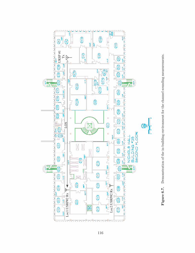
UR
SP
#1
Tx
Lo
c1
:US
RP
#2
Rx
LO
S
Lo
c2
:US
RP
#2
Rx
Fig
ure
6.7.
Dem
onst
rati
onof
the
in-b
uild
ing
envi
ronm
ent
for
the
chan
nels
ound
ing
mea
sure
men
ts.
116
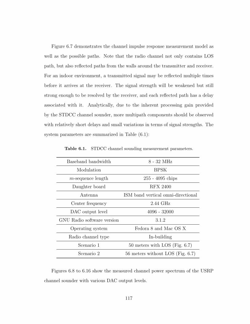
Figure 6.7 demonstrates the channel impulse response measurement model as
well as the possible paths. Note that the radio channel not only contains LOS
path, but also reflected paths from the walls around the transmitter and receiver.
For an indoor environment, a transmitted signal may be reflected multiple times
before it arrives at the receiver. The signal strength will be weakened but still
strong enough to be resolved by the receiver, and each reflected path has a delay
associated with it. Analytically, due to the inherent processing gain provided
by the STDCC channel sounder, more multipath components should be observed
with relatively short delays and small variations in terms of signal strengths. The
system parameters are summarized in Table (6.1):
Table 6.1. STDCC channel sounding measurement parameters.
Baseband bandwidth 8 - 32 MHz
Modulation BPSK
m-sequence length 255 - 4095 chips
Daughter board RFX 2400
Antenna ISM band vertical omni-directional
Center frequency 2.44 GHz
DAC output level 4096 - 32000
GNU Radio software version 3.1.2
Operating system Fedora 8 and Mac OS X
Radio channel type In-building
Scenario 1 50 meters with LOS (Fig. 6.7)
Scenario 2 56 meters without LOS (Fig. 6.7)
Figures 6.8 to 6.16 show the measured channel power spectrum of the USRP
channel sounder with various DAC output levels.
117
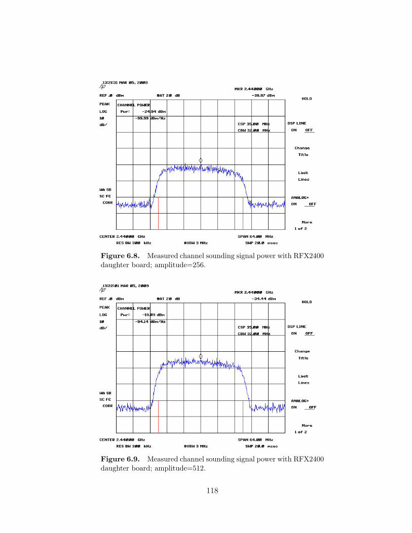
Figure 6.8. Measured channel sounding signal power with RFX2400daughter board; amplitude=256.
Figure 6.9. Measured channel sounding signal power with RFX2400daughter board; amplitude=512.
118

Figure 6.10. Measured channel sounding signal power withRFX2400 daughter board; amplitude=1024.
Figure 6.11. Measured channel sounding signal power withRFX2400 daughter board; amplitude=2048.
119
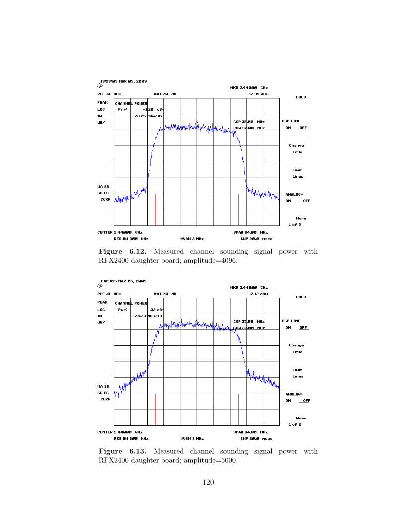
Figure 6.12. Measured channel sounding signal power withRFX2400 daughter board; amplitude=4096.
Figure 6.13. Measured channel sounding signal power withRFX2400 daughter board; amplitude=5000.
120

Figure 6.14. Measured channel sounding signal power withRFX2400 daughter board; amplitude=6000.
Figure 6.15. Measured channel sounding signal power withRFX2400 daughter board; amplitude=7000.
121

Figure 6.16. Measured channel sounding signal power withRFX2400 daughter board; amplitude=8000.
As we can see from the figures above, the signal sidelobe power level starts
to increase once the DAC output power level exceeds 4096, which is half of the
full DAC range. Performing channel sounding at such a power level will generate
unacceptable interference to the adjacent channel. Furthermore, the noise level
is also increased when boosting the signal power level. Besides interference, the
power amplifier nonlineararity also comes into play when the DAC is overdriven.
Figure 6.17 indicates that the channel power starts to saturate when the DAC
output level exceeds 4096. Overall, we chose a DAC output power level of 4096
to avoid unintended interference to the adjacent channel, as well as nonlineararity
distortion.
Figure 6.18 shows a comparison between the channel power and the DAC
output level for an m-sequence length varying from 512 to 4096. The measured
122

256 512 1,024 2,048 4096 6K 8K−40
−35
−30
−25
−20
−15
−10
−5
0
5
DAC Output level
Pow
er (
dB
m)
Channel PowerPower @ f
c
Figure 6.17. Relationship between the DAC output level and themeasured output power.
channel power for different sequence lengths is relatively close. The power at center
frequency behaves randomly comparing with the channel power consistency. This
is because the video averaging was turned off during measurement for accuracy. It
is also noticed that the actual output power for the channel sounding application
does not match the theoretical maximum output power for the RFX 2400 daughter
board. This can be caused by many factors, such as signal bandwidth, insertion
loss, other losses on the board, RF cable loss, measurement equipment loss, etc.
One example is the RF cable; the RG-58/U type cable has about 20 dB loss at
frequency higher than 1 GHz. The measured channel power is −32.86 and −1.2
dBm for DAC output level of 4096 respectively with RG-58/U and minibend W-8
cable.
In order to achieve the optimal SNR, the receiver gain needs to be tuned to
123

103
104
−50
−40
−30
−20
−10
0
DAC output level
Po
wer
(d
Bm
)
512
1024
2048
4096
power @ center frequency
Channel Power
Figure 6.18. Relationship between the DAC output level and chan-nel power; m-sequence length = 512, 1024, 2048, 4096.
the optimal value for a certain environment. Figures 6.19 to 6.23 illustrate the
maximum received channel impulse response power to noise power ratio versus
the receiver gain. The channel sounding sequence length is equal to 1023 chips,
and chip rate is 8 Mcps in this case. Each CIR takes approximately 0.13 second
to compute, and the total number of CIR set collected is equal to 100, hence, the
overall CIR calculation time is 13 seconds for each parameter set. The reason why
a 1023-chip m-sequence is chosen is because longer chip sequence requires much
longer calculation time. In addition, the multipath delay for indoor environment
is much shorter compared with the maximum delay that a long m-sequence can
offer. The rms delay spread for the indoor channel is on the order of nanoseconds,
while the maximum delay spread a 1023-chip m-sequence can detect is on the order
of microseconds for 8 Mcps.
124
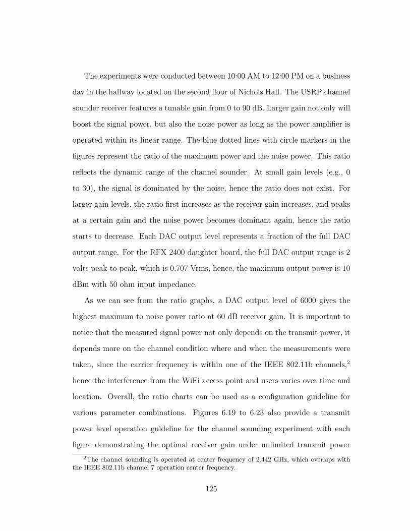
The experiments were conducted between 10:00 AM to 12:00 PM on a business
day in the hallway located on the second floor of Nichols Hall. The USRP channel
sounder receiver features a tunable gain from 0 to 90 dB. Larger gain not only will
boost the signal power, but also the noise power as long as the power amplifier is
operated within its linear range. The blue dotted lines with circle markers in the
figures represent the ratio of the maximum power and the noise power. This ratio
reflects the dynamic range of the channel sounder. At small gain levels (e.g., 0
to 30), the signal is dominated by the noise, hence the ratio does not exist. For
larger gain levels, the ratio first increases as the receiver gain increases, and peaks
at a certain gain and the noise power becomes dominant again, hence the ratio
starts to decrease. Each DAC output level represents a fraction of the full DAC
output range. For the RFX 2400 daughter board, the full DAC output range is 2
volts peak-to-peak, which is 0.707 Vrms, hence, the maximum output power is 10
dBm with 50 ohm input impedance.
As we can see from the ratio graphs, a DAC output level of 6000 gives the
highest maximum to noise power ratio at 60 dB receiver gain. It is important to
notice that the measured signal power not only depends on the transmit power, it
depends more on the channel condition where and when the measurements were
taken, since the carrier frequency is within one of the IEEE 802.11b channels,2
hence the interference from the WiFi access point and users varies over time and
location. Overall, the ratio charts can be used as a configuration guideline for
various parameter combinations. Figures 6.19 to 6.23 also provide a transmit
power level operation guideline for the channel sounding experiment with each
figure demonstrating the optimal receiver gain under unlimited transmit power
2The channel sounding is operated at center frequency of 2.442 GHz, which overlaps withthe IEEE 802.11b channel 7 operation center frequency.
125

level.
0 10 20 30 40 50 60 70 800
5
10
15
20
25
Receiver Gain (dB)
Rat
io o
f m
axim
um
po
wer
an
d n
ois
e p
ow
er
100*Pmax
Pm
/N0
Figure 6.19. Ratio of maximum received channel impulse responsepower and noise power; DAC output level=6000.
6.2.2 CIR Measurement Results and Analysis
The channel impulse response measurement results discussed in this section
were collected using the optimal parameters for the indoor environment, for which
the output DAC level is equal to 6000, and the receiver gain is set to be 60 dB.
Both line-of-sight and nonline-of-sight cases were measured at location one shown
in Figure 6.7. The LOS measurements were taken at location 1 and the non-LOS
measurements were taken at location 2 (see Figure 6.7). The m-sequence length is
1023, 4095 chips, chip rate is 8, 32 Mcps for both cases; the minimum delay
resolution is equal to 125, 31.25 ns respectively, and the maximum detectable
delay is approximately 128 µs for both sets. The total number of CIR snapshots
126
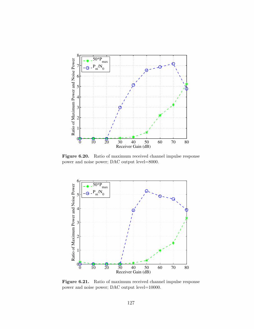
0 10 20 30 40 50 60 70 800
1
2
3
4
5
6
7
8
Receiver Gain (dB)
Rati
o o
f M
ax
imu
m P
ow
er
an
d N
ois
e P
ow
er
50*Pmax
Pm
/N0
Figure 6.20. Ratio of maximum received channel impulse responsepower and noise power; DAC output level=8000.
0 10 20 30 40 50 60 70 800
1
2
3
4
5
6
Receiver Gain (dB)
Rati
o o
f M
ax
imu
m P
ow
er
an
d N
ois
e P
ow
er
50*Pmax
Pm
/N0
Figure 6.21. Ratio of maximum received channel impulse responsepower and noise power; DAC output level=10000.
127

0 10 20 30 40 50 60 70 800
1
2
3
4
5
6
7
Receiver Gain (dB)
Rati
o o
f M
ax
imu
m P
ow
er
an
d N
ois
e P
ow
er
50*Pmax
Pm
/N0
Figure 6.22. Ratio of maximum received channel impulse responsepower and noise power; DAC output level=20000.
0 10 20 30 40 50 60 70 800
1
2
3
4
5
6
Receiver Gain (dB)
Rati
o o
f M
ax
imu
m P
ow
er
an
d N
ois
e P
ow
er
100*Pmax
Pm
/N0
Figure 6.23. Ratio of maximum received channel impulse responsepower and noise power; DAC output level=30000.
128

collected is 100, which allows us to generate an average power delay profile across
a time window width of 0.13 and 0.5 second for each sequence length. The mea-
surements will be conducted at two different chip rates; the slower chip rate is
essentially limited by the USB 2.0 throughput limitation (32 MB/s), as well as the
lowpass filter. The higher chip rate version uses a custom FPGA bitstream file to
bypass the USB 2.0 port when recording the channel impulse response measure-
ment data. In addition, the received data is not filtered by the 20 MHz baseband
filter, hence the maximum possible bandwidth is achieved.
6.2.2.1 Indoor Channel Measurement
Figures 6.24 and 6.25 display the measured channel impulse response for an
indoor environment at two different locations. Figure 6.24 clearly shows three
multipath channel components. The first path contains the most power. Notice
that the power of the second multipath component is not significantly smaller
than the first path. This is due to the fact that the measurement was conducted
in the hallway, where the reflected signal strength is not weakened dramatically.
However, if the signal is reflected multiple times before it reaches the receiver, the
signal strength can be undetectable. Although only three multipath components
were captured by the receiver, there might be more delay paths that fall in between
two delay paths, since the minimum delay resolution of the channel sounder is only
62.5 ns. As discussed previously, the delay for an indoor channel can be as small
as several nano seconds, which requires a channel sounder operating at 100 Mcps
or higher.
Figure 6.25 illustrates a channel impulse response measurement for a non-
LOS scenario. For this scenario, the first path that arrives at the reciever does
129

0 1 2 3 4 5 6 7
x 10−6
0
0.005
0.01
0.015
0.02
Relative Delay (s)
Mag
nit
ude
Figure 6.24. Measured channel impulse response with LOS; m-sequence length = 4095; chip rate = 32 Mcps.
not contain the strongest signal strength, because the signal is attenuated when
transmitting through obstacles, such as doors, walls, etc. The delay component
with the strongest signal strength usually takes a longer route where less obstacles
are in the path, hence the signal strength does not suffer from attenuation as much
as the first path. However, signal reflection can also cause signal strength reduc-
tion, which explains the reason why the magnitude is lower than in Figure 6.24.
Moreover, the signal magnitudes shown in those two figures are instantaneous,
which varies from one time instance to another. A better illustration will be the
power delay profile, which shows the average channel impulse response over a
period of measurement time.
Figures 6.26 and 6.27 demonstrate the power delay profile measurements for
the same indoor channel as Figures 6.24 and 6.25. The power delay profile is
obtained by averaging 100 CIR snapshots, which is approximately over a time
130
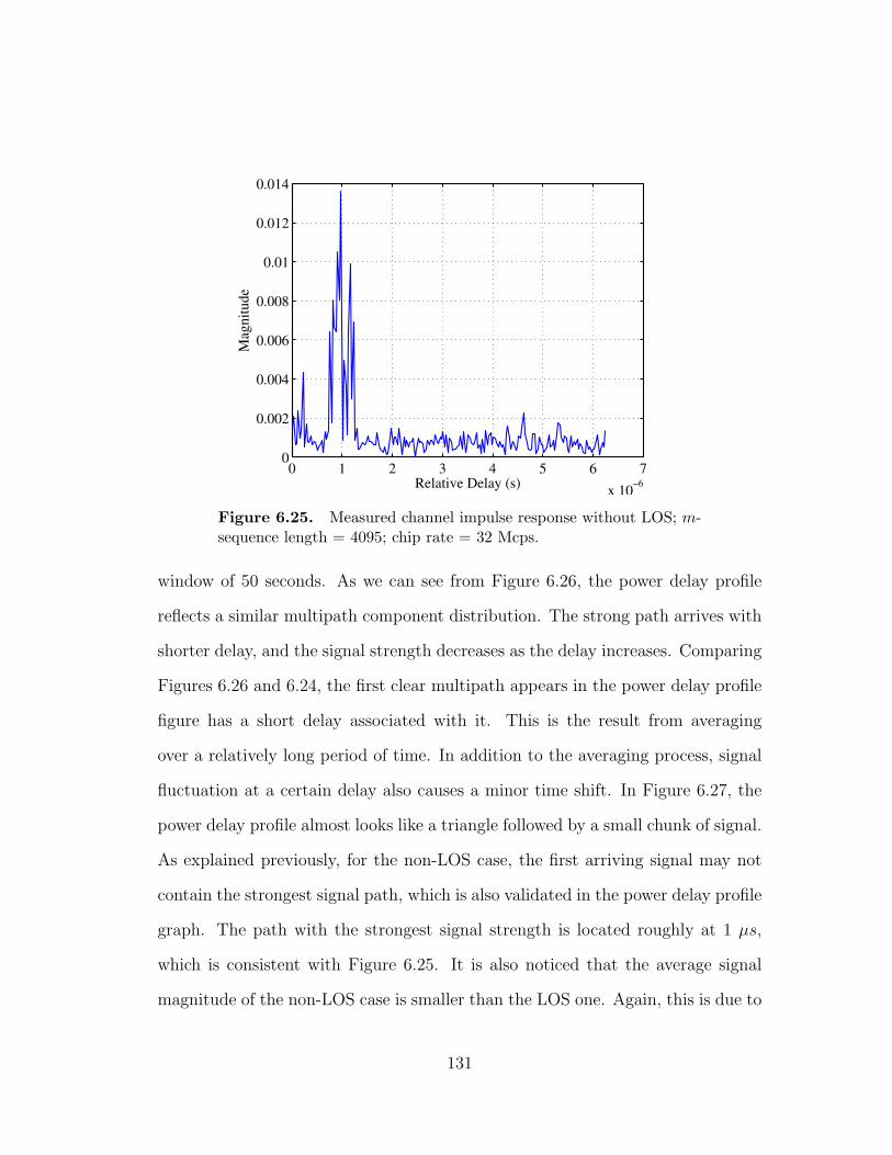
0 1 2 3 4 5 6 7
x 10−6
0
0.002
0.004
0.006
0.008
0.01
0.012
0.014
Relative Delay (s)
Mag
nit
ude
Figure 6.25. Measured channel impulse response without LOS; m-sequence length = 4095; chip rate = 32 Mcps.
window of 50 seconds. As we can see from Figure 6.26, the power delay profile
reflects a similar multipath component distribution. The strong path arrives with
shorter delay, and the signal strength decreases as the delay increases. Comparing
Figures 6.26 and 6.24, the first clear multipath appears in the power delay profile
figure has a short delay associated with it. This is the result from averaging
over a relatively long period of time. In addition to the averaging process, signal
fluctuation at a certain delay also causes a minor time shift. In Figure 6.27, the
power delay profile almost looks like a triangle followed by a small chunk of signal.
As explained previously, for the non-LOS case, the first arriving signal may not
contain the strongest signal path, which is also validated in the power delay profile
graph. The path with the strongest signal strength is located roughly at 1 µs,
which is consistent with Figure 6.25. It is also noticed that the average signal
magnitude of the non-LOS case is smaller than the LOS one. Again, this is due to
131

0 0.2 0.4 0.6 0.8 1
x 10−5
0
0.002
0.004
0.006
0.008
0.01
0.012
Relative Delay (sec)
Mag
nit
ude
Figure 6.26. Power delay profile of the indoor channel with LOS;Number of CIR snapshots = 100.
the fact that the non-LOS signal suffers more attenuation than the LOS signal.
The dynamic range for the LOS power delay profile is approximately 15 dB,
where it is 20 dB for the non-LOS case. Intuitively, the LOS signal strength
should be stronger than the non-LOS signal, and hence the dynamic range is
wider. However, this is true for the channel impulse response at a given time
instance, see Figure 6.24 and 6.25 for example, because the power delay profile is
the average of the CIRs over a period of measurement time so the dynamic range
varies from one measurement to another.
Moreover, during the measurement period, the USRP underrun may happen
randomly. USRP underrun happens if not enough samples are ready to send to
the USRP sink, while the USB is still reading in data, which causes undesired
data to be recorded. To overcome this issue, a mechanism that marks the channel
sounding cycle when USRP underrun happens is implemented, and hence, the
132

0 0.2 0.4 0.6 0.8 1
x 10−5
0
0.002
0.004
0.006
0.008
0.01
Relative Delay (sec)
Mag
nit
ude
Figure 6.27. Power delay profile of the indoor channel without LOS;Number of CIR snapshots = 100.
0 0.2 0.4 0.6 0.8 1 1.2
x 10−4
0
0.02
0.04
0.06
0.08
0.1
0.12
Relative Delay (sec)
Mag
nit
ude
Figure 6.28. Example of the output of the correlator when USRPunderrun happens.
133

recored data can be neglected during post processing. This issue is more notice-
able for the 8 Mcps sounder, since the cross-correlation is performed by the end
terminal (computer), not the FPGA. Figure 6.28 shows an example of the output
of the correlator when the USRP underrun happens. It is seen from the graph
that the output shows channel impulse response on the order of 10−4 second,
which is unlikely to happen for indoor environment. After an investigation of the
received signal, the output appears to be the correlation between the m-sequence
and random data, which contains out-of-order m-sequences.
6.2.2.2 Timing Offset Issue
The synchronization of TX and RX is a key problem for wireless channel
sounding. It is required to establish synchronization in frequency and time at
a TX and RX that can be separated by distances up to several kilometers. The
presence of multipath propagation makes this task even more difficult. For outdoor
environments, the Global Positioning System (GPS) offers a way of establishing
common time and frequency references [60]. However, this approach requires
a direct line of sight connection to GPS satellites which is rarely fullfilled in
microcellular scenarios. For the indoor channel sounding, distances up to about
10 meters, coaxial cable can be used to synchronize the TX and the RX. For larger
distances, fiber-optic cables are preferable.
As mentioned previously, time synchronization is not implemented for the
USRP, which will not only result in a time shift in the recorded channel impulse
response, but also a timing offset between the TX and RX local clock. Minor
timing offset will not affect the entire record of the CIR, however, high timing
offset will. The sounder works by transmitting a PN sequence, then correlating
134
the received sequence against the original at all possible offsets. However, to do
so, it collects an entire PN sequence and does the multiply and accumulate across
it for each lag in the impulse response. Thus, if the PN sequence period is N
chips, it takes N2 chips to calculate a single impulse response. For example, the
4095-chip sequence will take 16769025 chips to complete a single IR record. At 8
Mcps, this is approximately 2 seconds per record, and 0.5 second per record at 32
Mcps.
The crystal oscillator used by the USRP has an offset of ±50 ppm (parts per
million) between the transmitter and receiver. At 8 Mcps, during the course of 2
seconds, the receiver clock will differ from the transmit clock by:
2× 50× 10−6 × 86 = 800 chips, (6.2)
which is equivalent to 6400 clocks. At 32 Mcps, the timing offset between the TX
and RX is the same as 8 Mcps. Hence, the next peak in the correlation will arrive
800 chips earlier at 50 ppm, which results in a compressed correlation bin. To
prove the effect of timing offset between TX and RX, Fgure 6.29 shows a record
of the channel impulse resopnse with compressed correlation bin size.
Figure 6.29(a) is generated by using a 4095-chip PN sequence, the correlation
peak separation should be 4095 chips with perfect timing synchronization. How-
ever, due to timing offset, the correlation peak offset becomes 800 chips. Both
Figures 6.29(a) and 6.29(b) show a compressed correlation bin size of 800 chips.
For both cases, the correlation bin size is compressed to 800 chips, so the frequency
offset of the crystal oscillator is 50 ppm.
Based on the analysis, the sounder will not work for a PN sequence length
135

0 1000 2000 3000 4000 5000 60000
0.005
0.01
0.015
0.02
0.025
0.03
0.035
X: 2389
Y: 0.01938
X: 3189
Y: 0.02424
Chips
Mag
nit
ud
eX: 3994
Y: 0.03309
X: 4796
Y: 0.02011
(a) 32 Mcps timing offset.
0 1000 2000 3000 4000 5000 60000
0.02
0.04
0.06
0.08
0.1
0.12
X: 542
Y: 0.09337
X: 1347
Y: 0.06152
X: 2145
Y: 0.0667
Chips
Mag
nit
ud
e
X: 2950
Y: 0.1137
X: 3749
Y: 0.08217X: 4551
Y: 0.08119
X: 5352
Y: 0.1102
(b) 8 Mcps timing offset.,
Figure 6.29. Compressed correlation bin size for 8 and 32 Mcps; PNsequence length is 4095 and 1023 chips for 32 and 8 Mcps respectively.
136
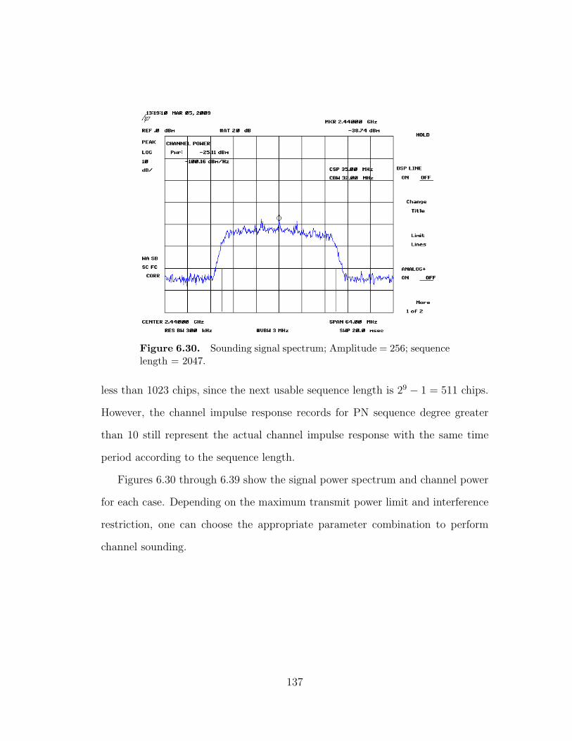
Figure 6.30. Sounding signal spectrum; Amplitude = 256; sequencelength = 2047.
less than 1023 chips, since the next usable sequence length is 29 − 1 = 511 chips.
However, the channel impulse response records for PN sequence degree greater
than 10 still represent the actual channel impulse response with the same time
period according to the sequence length.
Figures 6.30 through 6.39 show the signal power spectrum and channel power
for each case. Depending on the maximum transmit power limit and interference
restriction, one can choose the appropriate parameter combination to perform
channel sounding.
137

Figure 6.31. Sounding signal spectrum; Amplitude = 512; sequencelength = 2047.
Figure 6.32. Sounding signal spectrum; Amplitude = 1024; se-quence length = 2047.
138

Figure 6.33. Sounding signal spectrum; Amplitude = 2048; se-quence length = 2047.
Figure 6.34. Sounding signal spectrum; Amplitude = 4096; se-quence length = 2047.
139
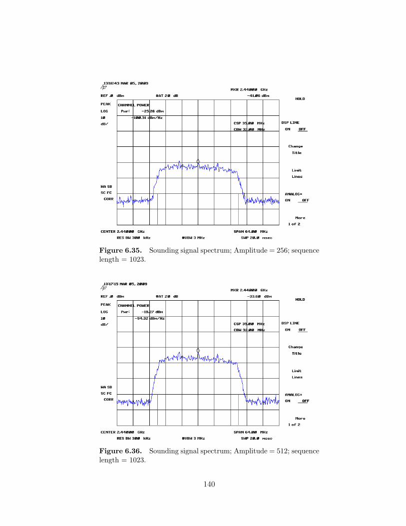
Figure 6.35. Sounding signal spectrum; Amplitude = 256; sequencelength = 1023.
Figure 6.36. Sounding signal spectrum; Amplitude = 512; sequencelength = 1023.
140

Figure 6.37. Sounding signal spectrum; Amplitude = 1024; se-quence length = 1023.
Figure 6.38. Sounding signal spectrum; Amplitude = 2048; se-quence length = 1023.
141
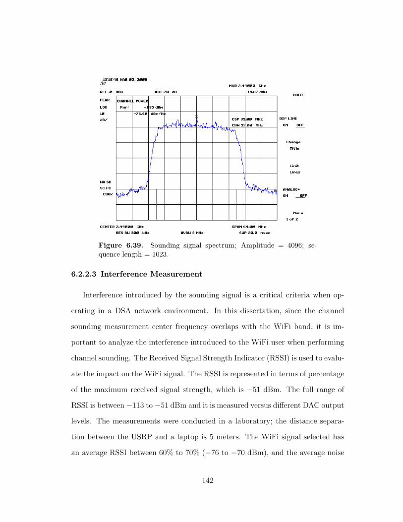
Figure 6.39. Sounding signal spectrum; Amplitude = 4096; se-quence length = 1023.
6.2.2.3 Interference Measurement
Interference introduced by the sounding signal is a critical criteria when op-
erating in a DSA network environment. In this dissertation, since the channel
sounding measurement center frequency overlaps with the WiFi band, it is im-
portant to analyze the interference introduced to the WiFi user when performing
channel sounding. The Received Signal Strength Indicator (RSSI) is used to evalu-
ate the impact on the WiFi signal. The RSSI is represented in terms of percentage
of the maximum received signal strength, which is −51 dBm. The full range of
RSSI is between −113 to −51 dBm and it is measured versus different DAC output
levels. The measurements were conducted in a laboratory; the distance separa-
tion between the USRP and a laptop is 5 meters. The WiFi signal selected has
an average RSSI between 60% to 70% (−76 to −70 dBm), and the average noise
142

0 20 40 60 80
30
40
50
60
70
80
Sample Index
RS
SI
Per
centa
ge
(%)
8000
512
1024
Figure 6.40. Impact on the RSSI of a WiFi signal during channelsounding measurement.
level for this location is −111.2 dBm, which is equivalent to 4% of the maximum
RSSI.
Figure 6.40 shows a comparison between the impact on the RSSI for a DAC
output level of 512, 1024, and 8000. The X-axis denotes the RSSI measurement
sample index, where, theY-axis is the RSSI in percentage. The RSSI is measured
during a period in which the channel sounder is turned on and off and turned on
again. As we can observe from the figure, when the channel sounder is transmitting
at the highest power (refer to Figure 6.16), the the RSSI increases about 40%
from interference to interference-free.3 For lower sounding signal power levels, the
RSSI drop is approximately 12% and 15% for DAC output levels of 512 and 1024,
respectively.
3We only consider interference from the sounding signal. Other interference sources are notdiscussed here.
143
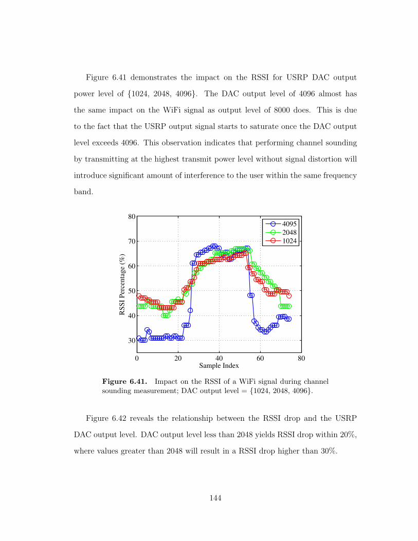
Figure 6.41 demonstrates the impact on the RSSI for USRP DAC output
power level of 1024, 2048, 4096. The DAC output level of 4096 almost has
the same impact on the WiFi signal as output level of 8000 does. This is due
to the fact that the USRP output signal starts to saturate once the DAC output
level exceeds 4096. This observation indicates that performing channel sounding
by transmitting at the highest transmit power level without signal distortion will
introduce significant amount of interference to the user within the same frequency
band.
0 20 40 60 80
30
40
50
60
70
80
Sample Index
RS
SI
Per
centa
ge
(%)
4095
2048
1024
Figure 6.41. Impact on the RSSI of a WiFi signal during channelsounding measurement; DAC output level = 1024, 2048, 4096.
Figure 6.42 reveals the relationship between the RSSI drop and the USRP
DAC output level. DAC output level less than 2048 yields RSSI drop within 20%,
where values greater than 2048 will result in a RSSI drop higher than 30%.
144
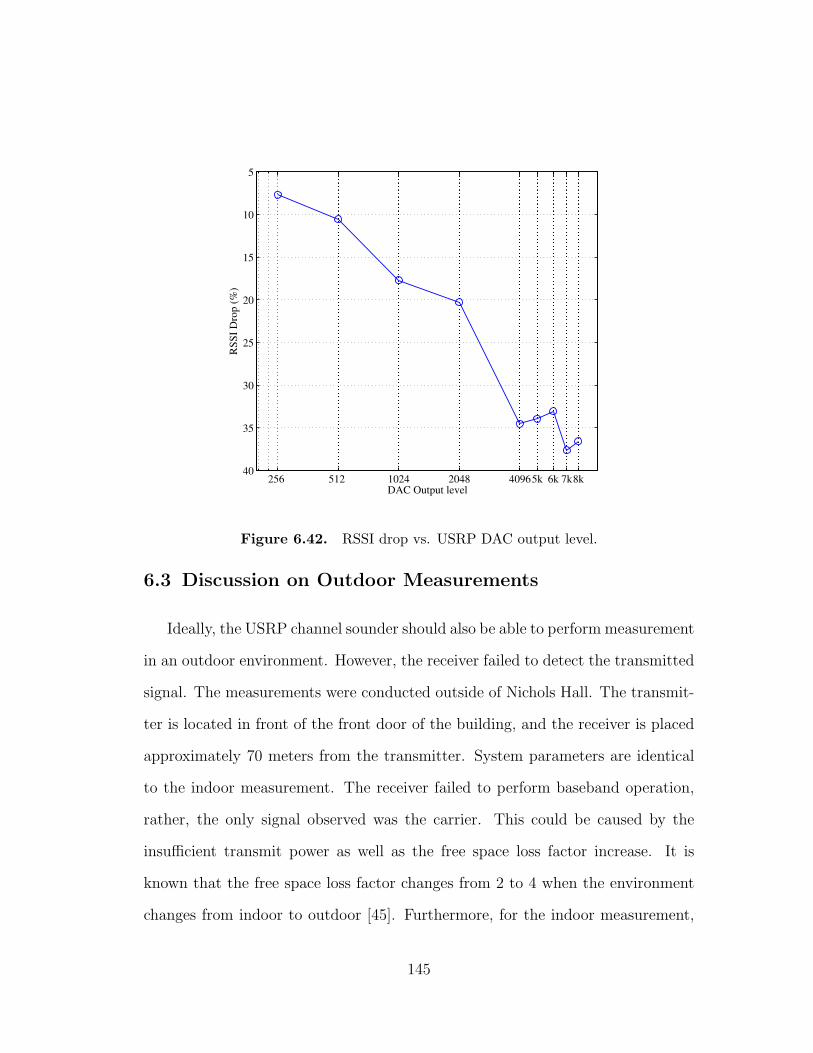
256 512 1024 2048 40965k 6k 7k8k40
35
30
25
20
15
10
5
DAC Output level
RS
SI
Dro
p (
%)
Figure 6.42. RSSI drop vs. USRP DAC output level.
6.3 Discussion on Outdoor Measurements
Ideally, the USRP channel sounder should also be able to perform measurement
in an outdoor environment. However, the receiver failed to detect the transmitted
signal. The measurements were conducted outside of Nichols Hall. The transmit-
ter is located in front of the front door of the building, and the receiver is placed
approximately 70 meters from the transmitter. System parameters are identical
to the indoor measurement. The receiver failed to perform baseband operation,
rather, the only signal observed was the carrier. This could be caused by the
insufficient transmit power as well as the free space loss factor increase. It is
known that the free space loss factor changes from 2 to 4 when the environment
changes from indoor to outdoor [45]. Furthermore, for the indoor measurement,
145

the propagation channel can be considered as a tunnel, where the reflected signals
are bounded within the tunnel. For outdoor environment, since onmi-directional
antenna is used, the signal is emitted in all directions, which can cause weak signal
strength at the receiver.
Based on the analysis, some suggestions can be made for ourdoor measure-
ments.
• Directional Antenna: Directional antennas can limit the radiation to a nar-
row angle so that the signal strength is enhanced. As mentioned previously,
for indoor channels, the signal is traversing through a relatively narrow space
comparing with outdoor channels. The signal might be reflected multiple
times before it is received by the receiver. The outcome is a channel impulse
response with a large number of multipath components compacted together.
• Carrier Synchronization: Carrier Synchronization plays a more important
role in outdoor channels because of greater Doppler shift. Large transmitter
and receiver carrier frequency offset can result in signal reception failure. It
is more severe for the sliding correlator based channel sounding, because the
receiver is very likely to correlate with an undesired signal.
• Gain: In general, for an outdoor radio channel, signal distortion is more
severe than for an indoor channel. This is because the objects in the channel
are more scattered, and hence the signal attenuation and phase rotation are
worse than for an indoor channel.
146

6.4 Chapter Summary
In this chapter, the implementation of the swept-time delay cross correlation
channel sounder is presented. The STDCC channel sounder is implemented based
on the USRP hardware platform with maximum bandwidth of 32 MHz, and an
m-sequence length of 4095 chips. To achieve the maximum available bandwidth,
a custom FPGA bitstream file is used in order to bypass the USB port band-
width limitation. The GNU radio software is used to build the transmitter and
receiver as well as the signal processing function blocks. Indoor channel sound-
ing measurements were conducted inside Nichols Hall. Both line-of-sight and
nonline-of-sight scenarios were studied, and measurement results were analyzed.
Interference measurements were also conducted by measuring the RSSI drop of a
nearby WiFi signal. The measurements show that the channel sounder will intro-
duce significant amount interference when transmitting at half of the maximum
power. However, this issue can be solved if the MC-DS-STDCC sounder is used.
The experiment is not intended to be used to study the indoor wireless channel
behavior because of it’s lack of bandwidth. It is rather a preliminary implemen-
tation and measurement for later research. Unlike most commercial products,
the GNU radio and USRP are still in the research stage, and many software and
hardware issues are to be discovered by researchers.
147

Chapter 7
Conclusion
7.1 Research Achievements
Channel sounding plays a critical role in wireless system design. It provides
the designer knowledge of the radio channel in assisting system design in many
degrees. It also provides a route to study the characteristics of the radio channel,
which can be used in simulation and channel modeling. In this dissertation, the
challenges of designing a channel sounding technique for the dynamic spectrum
access network are presented. Due to the randomness of spectral and temporal
access of the DSA network, performing channel sounding consistently without
interfering with other users becomes the major design concern.
The major contributions of this dissertations are summarized as following:
• Characterized the user access randomness in both frequency and time do-
main. Explicitly, unlicensed users access the channel, depending more on
the channel availability and interference tolerance level compared to the li-
censed users. The licensed users can access the channel without realizing
the existence of the unlicensed users. Addressed challenges in designing the
148

channel sounding system for the DSA network environment. Tasks need-
ing to be solved are how to perform channel sounding without interfering
with other users; how to perform channel sounding efficiently when frequent
frequency and time switching is required.
• A multicarrier direct sequence spreading based channel sounding system
framework combining with the STDCC channel sounder, also termed as
MC-DS-STDCC is presented. The MC-DS-STDCC utilizes direct sequence
spreading to minimize the interference to other users within the same fre-
quency band, and multicarrier modulation to achieve frequency agility. To
be more specific, each subcarrier is able to adjust the transmit power by
increasing or decreasing the spreading sequence length in order to satisfy
the power limit. Moreover, the use of spread spectrum also increases the
inherent processing gain of the system, and hence, the dynamic range of the
channel sounder is enlarged.
• In contrast to the MC-DS-STDCC channel sounding technique, the OFDM-
based channel sounding technique is focusing on reducing the system com-
plexity, mainly sampling rate. The OFDM-based channel sounder uses has
the ability to use the user data as the sounding signal, which eliminates
the sounding signal generator, and hence the system complexity is reduced.
However, the performance is directly related to the autocorrelation of the
user transmit data, that is, the optimal sounding signal is achieved when the
data across all subcarriers is equal to one. A tradeoff study is conducted in
interpolating the performance loss versus the randomness of the user data.
On the other hand, since the OFDM-based channel sounding technique uses
149

user data as the sounding signal, no extra interference will be introduced as
long as the user has permission to the frequency band. However, the system
performance is traded off for the system complexity.
• Channel sounder is a measurement device, and hence, it is only useful if
implemented. In this dissertation, the implementation of the STDCC is
presented based on the USRP and GNU radio. The implementation of the
MC-DS-STDCC and OFDM-based channel sounder is out of the scope of this
dissertation because of the hardware and software limitation. The USRP
platform supports maximum bandwidth of 32 MHz by adopting a custom
FPGA bitstream file to bypass the bandpass filter built-in on the daughter
board. This bandwidth limitation is the major obstacle of implementing the
MC-DS-STDCC channel sounder, which requires a much higher bandwidth
in order to perform spread spectrum. Indoor experiments were conducted
inside Nichols Hall in Lawrence, KS. The experiment results were studied
and analyzed.
7.2 Future Work
There exists a number of topics that have resulted from this research that are
worth continuing:
• Towards the end of this research, the second version of the USRP became
available, which supports much higher baseband bandwidth and eliminates
the USB bottleneck completely by replacing it with a gigabyte Ethernet
interface. This improvement makes the implementation of the MC-DS-
STDCC and OFDM-based channel sounder become feasible. It would be
150

interesting to implement both proposed systems on the USRP 2.
• The channel sounding measurements taken were for the static channel envi-
ronment, for most of the modern wireless communication system, the trans-
mitter and receiver are nonstatic, which means the study of the Doppler
shift is essential. Again, the USRP 2 allows us to upload the GNU radio
software onto the board, which makes the entire unit stand alone. This
makes the study of the Doppler shift doable.
• Due to the randomness of the DSA network, predicting the channel behavior
becomes difficult. A long term statistical analysis of the channel behavior
would be invaluable for both channel modeling and system design. This
work requires the development of a signal processing algorithm to process
the collected data.
151

References
[1] J. Mitola, “Software radio architecture: a mathematical perspective,” Se-
lected Areas in Communications, IEEE Journal on, vol. 17, no. 4, pp. 514–
538, 1999.
[2] J. Parsons, D. Demery, and A. Turkmani, “Sounding techniques for wideband
mobile radio channels: a review,” in Communications, Speech and Vision,
IEE Proceedings I, vol. 138, October 1991, pp. 437–446.
[3] D. Cox and R. Leck, “Correlation bandwidth and delay spread multipath
propagation statistics for 910-MHz urban mobile radio channels,” Communi-
cations, IEEE Transactions on, vol. 23, no. 11, pp. 1271 – 1280, Jan 1975.
[4] D. Cox, “Delay doppler characteristics of multipath propagation at 910 MHz
in a suburban mobile radio environment,” Antennas and Propagation, IEEE
Transactions on, vol. 20, no. 5, pp. 625 – 635, Jan 1972.
[5] D. Cox and R. Leck, “Distributions of multipath delay spread and average
excess delay for 910-MHz urban mobile radio paths,” Antennas and Propa-
gation, IEEE Transactions on, vol. 23, no. 2, pp. 206 – 213, Jan 1975.
152

[6] D. Cox, “A measured delay-doppler scattering function for multipath prop-
agation at 910 MHz in an urban mobile radio environment,” Proceedings of
the IEEE, vol. 61, no. 4, pp. 479– 480, 1973.
[7] “FCC statement of the chairman.” [Online]. Available: http://www.fcc.gov/
Daily Releases/Daily Business/2008/db1117/FCC-08-260A2.txt
[8] “DARPA XG Program web site.” [Online]. Available: http://www.darpa.
mil/ato/programs/XG/
[9] “OverDRiVE web site.” [Online]. Available: http://www.ist-drive.org/
index2.html
[10] D. Grandblaise, D. Bourse, K. Moessner, and P. Leaves, “Dynamic Spectrum
Allocation (DSA) and Reconfigurability,” in SDR Forum, November 2002.
[11] J. Parsons, D. Demery, and A. Turkmani, “Sounding techniques for wideband
mobile radio channels: a review,” Communications, Speech and Vision, IEE
Proceedings I, vol. 138, no. 5, pp. 437 – 446, Oct 1991.
[12] “Ettus Research web site.” [Online]. Available: http://www.ettus.com
[13] A. Healey, C. Bianchi, and K. Sivaprasad, “Wideband outdoor channel sound-
ing at 2.4 ghz,” Antennas and Propagation for Wireless Communications,
2000 IEEE-APS Conference on, pp. 95 – 98, Oct 2000.
[14] J. Kivinen, T. Korhonen, P. Aikio, R. Gruber, P. Vainikainen, and S. Hag-
gman, “Wideband radio channel measurement system at 2 ghz,” Instrumen-
tation and Measurement, IEEE Transactions on, vol. 48, no. 1, pp. 39 – 44,
Feb 1999.
153
[15] S. Salous and V. Hinostroza, “Wideband indoor frequency agile channel
sounder and measurements,” Microwaves, Antennas and Propagation, IEE
Proceedings -, pp. 573 – 580, Nov 2005.
[16] R. Thoma, M. Landmann, G. Sommerkorn, and A. Richter, “Multidimen-
sional high-resolution channel sounding in mobile radio,” Instrumentation
and Measurement Technology Conference, 2004. IMTC 04. Proceedings of
the 21st IEEE, vol. 1, pp. 257 – 262 Vol.1, Apr 2004.
[17] S. Charles, E. Ball, T. Whittaker, and J. Pollard, “Channel sounder for 5.5
ghz wireless channels,” Communications, IEE Proceedings-, vol. 150, no. 4,
pp. 253 – 258, Jul 2003.
[18] R. Thoma, D. Hampicke, A. Richter, and G. Sommerkorn, “Measurement
and identification of mobile radio propagation channels,” Instrumentation
and Measurement Technology Conference, 2001. IMTC 2001. Proceedings of
the 18th IEEE, vol. 2, pp. 1163 – 1170 vol.2, Apr 2001.
[19] T. Takeuchi and M. Tamura, “A ultra-wide band channel sounder for mobile
communication systems,” Personal, Indoor and Mobile Radio Communica-
tions, 2001 12th IEEE International Symposium on, vol. 2, pp. E–111 – E–115
vol.2, Jan 2001.
[20] S. Haese, C. Moullec, P. Coston, and K. Sayegrih, “Wideband measure-
ments of the outdoor propagation channel using a new time domain channel
sounder,” Vehicular Technology Conference, 1999. VTC 1999 - Fall. IEEE
VTS 50th, vol. 4, pp. 2248 – 2252 vol.4, Aug 1999.
154
[21] S. Guillouard, G. E. Zein, and J. Citerne, “Wideband propagation measure-
ments and doppler analysis for the 60 ghz indoor channel,” Microwave Sym-
posium Digest, 1999 IEEE MTT-S International, vol. 4, pp. 1751 – 1754
vol.4, May 1999.
[22] S. Haese, C. Moullec, P. Coston, and K. Sayegrih, “High-resolution spread
spectrum channel sounder for wireless communications systems,” Personal
Wireless Communication, 1999 IEEE International Conference on, pp. 170
– 173, Jan 1999.
[23] U. Karthaus and R. Noe, “Results of extensive 800 mb/s, 30 ghz chan-
nel sounding experiments,” Antennas and Propagation Society International
Symposium, 1998. IEEE, vol. 3, pp. 1688 – 1691 vol.3, May 1998.
[24] J. Kivinen and P. Vainikainen, “Wideband propagation measurements in cor-
ridors at 5.3 ghz,” Spread Spectrum Techniques and Applications, 1998. Pro-
ceedings., 1998 IEEE 5th International Symposium on, vol. 2, pp. 512–516
vol.2, 1998.
[25] P. Karlsson, C. Bergljung, E. Thomsen, and H. Borjeson, “Wideband mea-
surement and analysis of penetration loss in the 5 ghz band,” Vehicular Tech-
nology Conference, 1999. VTC 1999 - Fall. IEEE VTS 50th, vol. 4, pp. 2323–
2328 vol.4, 1999.
[26] J. Andersen, T. Rappaport, and S. Yoshida, “Propagation measurements and
models for wireless communications channels,” Communications Magazine,
IEEE, vol. 33, no. 1, pp. 42–49, 1995.
155

[27] J. Medbo, H. Hallenberg, and J.-E. Berg, “Propagation characteristics at 5
ghz in typical radio-lan scenarios,” Vehicular Technology Conference, 1999
IEEE 49th, vol. 1, pp. 185–189 vol.1, 1999.
[28] T. Rappaport, S. Seidel, and R. Singh, “900 mhz multipath propagation
measurements for us digital cellular radiotelephone,” Global Telecommunica-
tions Conference, 1989, and Exhibition. ’Communications Technology for the
1990s and Beyond’. GLOBECOM ’89., IEEE, pp. 84–89 vol.1, 1989.
[29] M. Madkour, S. Gupta, and Y. Wang, “Successive interference cancellation al-
gorithms for downlink w-cdma communications,” Wireless Communications,
IEEE Transactions on, vol. 1, no. 1, pp. 169 – 177, Jan 2002.
[30] T. Rondeau, C. Rieser, T. Gallagher, and C. Bostian, “Online modeling of
wireless channels with hidden markov models and channel impulse responses
for cognitive radios,” Microwave Symposium Digest, 2004 IEEE MTT-S In-
ternational, vol. 2, pp. 739 – 742 Vol.2, May 2004.
[31] A. Marousis, P. Karamalis, A. Kanatas, and P. Constantinou, “Design and
simulation of a vector channel sounder for umts,” Vehicular Technology Con-
ference, 2001. VTC 2001 Spring. IEEE VTS 53rd, vol. 1, pp. 382 – 386 vol.1,
Apr 2001.
[32] G. German, Q. Spencer, L. Swindlehurst, and R. Valenzuela, “Wireless in-
door channel modeling: statistical agreement of ray tracing simulations and
channel sounding measurements,” Acoustics, Speech, and Signal Processing,
2001. Proceedings. (ICASSP ’01). 2001 IEEE International Conference on,
vol. 4, pp. 2501 – 2504 vol.4, Apr 2001.
156
[33] R. Vaughan and N. Scott, “Super-resolution of pulsed multipath channels
for delay spread characterization,” Communications, IEEE Transactions on,
vol. 47, no. 3, pp. 343 – 347, Mar 1999.
[34] S. Mangold, M. Lott, D. Evans, and R. Fifield, “Indoor radio channel
modeling-bridging from propagation details to simulation,” Personal, Indoor
and Mobile Radio Communications, 1998. The Ninth IEEE International
Symposium on, vol. 2, pp. 625 – 629 vol.2, Aug 1998.
[35] L. Dossi, G. Tartara, and F. Tallone, “Statistical analysis of measured im-
pulse response functions of 2.0 ghz indoor radio channels,” Selected Areas in
Communications, IEEE Journal on, vol. 14, no. 3, pp. 405–410, 1996.
[36] W. Mohr, “Modeling of wideband mobile radio channels based on propagation
measurements,” Personal, Indoor and Mobile Radio Communications, 1995.
PIMRC’95. ’Wireless: Merging onto the Information Superhighway’., Sixth
IEEE International Symposium on, vol. 2, pp. 397–401 vol.2, 1995.
[37] P. Bello, “Characterization of randomly time-variant linear channels,” Com-
munications, IEEE Transactions on, vol. 11, no. 4, pp. 360– 393, 1963.
[38] G. Martin, “Wideband channel sounding dynamic range using a sliding cor-
relator,” Vehicular Technology Conference Proceedings, 2000. VTC 2000-
Spring Tokyo. 2000 IEEE 51st, vol. 3, pp. 2517 – 2521 vol.3, Apr 2000.
[39] A. Parr, B. Cho, and Z. Ding, “A new uwb pulse generator for fcc spectral
masks,” Vehicular Technology Conference, 2003. VTC 2003-Spring. The 57th
IEEE Semiannual, vol. 3, pp. 1664 – 1666 vol.3, Mar 2003.
157

[40] M. Hamalainen, A. Nykanen, V. Hovinen, and P. Leppanen, “Digital step-
ping correlator in a wideband radio channel measurement system,” Personal,
Indoor and Mobile Radio Communications, 1997. ’Waves of the Year 2000’.
PIMRC ’97., The 8th IEEE International Symposium on, vol. 3, pp. 1120 –
1124 vol.3, Aug 1997.
[41] R. J. Pirkl and G. D. Durgin, “How to build an optimal broadband channel
sounder,” Antennas and Propagation International Symposium, 2007 IEEE,
pp. 601 – 604, May 2007.
[42] A. Durantini, W. Ciccognani, and D. Cassioli, “Uwb propagation measure-
ments by pn-sequence channel sounding,” Communications, 2004 IEEE In-
ternational Conference on, vol. 6, pp. 3414 – 3418 Vol.6, May 2004.
[43] A. Levy, J. Rossi, J. Barbot, and J. Martin, “An improved channel sounding
technique applied to wideband mobile 900 MHz propagation measurements,”
Vehicular Technology Conference, 1990 IEEE 40th, pp. 513 – 519, Apr 1990.
[44] J. Austin, W. Ditmar, W. K. Lam, E. Vilar, and K. W. Wan;, “A spread
spectrum communications channel sounder,” Communications, IEEE Trans-
actions on, vol. 45, no. 7, pp. 840 – 847, Jul 1997.
[45] T. Rappaport, Wireless Communications: Principles and Practice. Prentice
Hall, 1996.
[46] M. Jeruchim, P. Balahan, and K. Shanmugan, Simulation of Communi-
cation Systems: Modeling, Methodoloty, and Techniques. Kluwer Aca-
demic/Plenum Publishers, 2000.
158
[47] P. Bello, “Characterization of Randomly Time-Variant Linear Channels,”
IEEE Transactions On Communication Systems, vol. 11, pp. 360–393, De-
cember 1963.
[48] G. Durgin, Space-Time Wireless Channels. Prentice Hall, 2003.
[49] “FCC part 15b regulations on U-NII band.” [Online]. Available:
http://www.atcb.com/publicdocs/fcc-03-287a1-UNII-Changes.pdf
[50] “ITU page on definitions of ISM bands.” [Online]. Available: http:
//www.itu.int/ITU-R/terrestrial/faq/index.html
[51] A. Hewitt and E. Vilar, “Selective fading on los microwave links: classi-
cal and spread-spectrum measurement techniques,” Communications, IEEE
Transactions on, vol. 36, no. 7, pp. 789–796, 1988.
[52] P. Smulders and A. Wagemans, “Frequency-domain measurement of the mil-
limeter wave indoor radio channel,” Instrumentation and Measurement, IEEE
Transactions on, vol. 44, no. 6, pp. 1017–1022, 1995.
[53] J. Parsons, The Mobile Radio Propagation Channel. John Wiley & Sons,
Inc.,, 2000.
[54] R. Dixon, Spread Spectrum Systems, 2nd ed. John Wiley & Sons, Inc., 1984.
[55] J. Meel, “Spread spectrum (SS),” De Nayer Instituut, Hogeschool Voor
Wetenschap & Kunst, December 1999.
[56] P. Karlsson and L. Olsson, “Time dispersion measurement system for radio
propagation at 1800 MHz and results from typical indoor environments,” Ve-
hicular Technology Conference, 1994 IEEE 44th, pp. 1793–1797 vol.3, 1994.
159

[57] Y. D. Jong and M. Herben, “High-resolution angle-of-arrival measurement
of the mobile radio channel,” Antennas and Propagation, IEEE Transactions
on, vol. 47, no. 11, pp. 1677–1687, 1999.
[58] G. J. Minden, J. B. Evans, L. Searl, D. DePardo, R. Rajbanshi, J. Guffey,
Q. Chen, T. Newman, V. R. Petty, F. Weidling, M. Lehnherr, B. Cordill,
D. Datla, B. Barker, and A. Agah, “An agile radio for wireless innovation,”
May 2007.
[59] A. Levy, J.-P. Rossi, J.-P. Barbot, and J. Martin, “An improved channel
sounding technique applied to wideband mobile 900 MHz propagation mea-
surements,” MAY 1990.
[60] A. F. Molisch, Wireless Communications. John Wiley & Sons, Inc., 2005.
[61] S. Hara and R. Prasad, “Overview of multicarrier CDMA,” Communications
Magazine, IEEE, vol. 35, no. 12, pp. 126–133, 1997.
[62] “3GPP Specifications Home Page.” [Online]. Available: http://www.3gpp.
org/specs/specs.htm
[63] T. Inoue, D. Garg, and F. Adachi, “Study of the OVSF Code Selection for
Downlink MC-CDMA,” IEICE Transactions on Communications, vol. E88-
B, pp. 499–508, Feburary 2005.
[64] L. Henzo, M. Munster, B. Choi, and T. Keller, OFDM and MC-CDMA for
Broadband Multi-User Communications, WLANs and Broadcasting. John
Wiley & Sons, Inc., 2003.
160

[65] N. Yee, J. Linnartz, and G. Fettweis, “Multicarrier CDMA in indoor wireless
radio netwokrs,” in PIMRC, September 1993, pp. 109–113.
[66] R. Peterson, R. Ziemer, and D. Borth, Introduction to Spread Spectrum Com-
munications. Prentice Hall, 1995.
[67] D. Sarwate and M. Pursley, “Crosscorrelation properties of pseudorandom
and related sequences,” Proceedings of the IEEE, vol. 68, no. 5, pp. 593–619,
May 1980.
[68] D. Sarwate, “Bounds on crosscorrelation and autocorrelation of sequences
(corresp.),” Information Theory, IEEE Transactions on, vol. 25, no. 6, pp.
720–724, Nov 1979.
[69] D. Sarwate and M. Pursley, “Crosscorrelation properties of pseudorandom
and related sequences,” Proceedings of the IEEE, vol. 68, no. 5, pp. 593–619,
May 1980.
[70] “Federal communications commission (FCC).” [Online]. Available: http:
//www.fcc.org
[71] A. Molina, P. Fannin, and J. Timoney, “Generation of optimum excitation
waveforms for mobile radio channel sounding,” Vehicular Technology, IEEE
Transactions on, vol. 44, no. 2, pp. 275–279, 1995.
[72] T. Felhauer, P. Baier, W. Konig, and W. Mohr, “Optimum spread spectrum
signals for wideband channel sounding,” Electronics Letters, vol. 29, no. 6,
pp. 563–564, 1993.
161

[73] Q. Shi and M. Latva-aho, “An exact error floor for downlink mc-cdma in
correlated rayleigh fading channels,” Communications Letters, IEEE, vol. 6,
no. 5, pp. 196–198, May 2002.
[74] A. Coulson, “Bit error rate performance of ofdm in narrowband interference
with excision filtering,” Wireless Communications, IEEE Transactions on,
vol. 5, no. 9, pp. 2484–2492, September 2006.
[75] U. Goni and A. Turkmani, “Ber performance of a direct-sequence cdma sys-
tem in multipath fading mobile radio channels with rake reception,” Jun
1994, pp. 747–751 vol.2.
[76] H. Xie, X. Wang, A. Wang, B. Qin, H. Chen, and B. Zhao, “An ultra low-
power low-cost gaussian impulse generator for uwb applications,” Solid-State
and Integrated Circuit Technology, 2006. ICSICT ’06. 8th International Con-
ference on, pp. 1817 – 1820, Sep 2006.
[77] W. Ye-Qiu, L. Ying-Hua, Z. Hong-Xin, and H. Peng-Fei;, “Evaluation of uwb
interference to the 3rd generation communication systems,” Environmental
Electromagnetics, The 2006 4th Asia-Pacific Conference on, pp. 161 – 164,
Jul 2006.
[78] B. T. Ahmed, M. C. Ramon, and L. H. Ariet, “On the impact of ultra
wide band (uwb) system on macrocell downlink of is-136 systems,” Wireless
Communication Systems, 2006. ISWCS ’06. 3rd International Symposium
on, pp. 645 – 649, Aug 2006.
[79] S. Brandes, I. Cosovic, and M. Schnell, “Sidelobe suppression in ofdm systems
by insertion of cancellation carriers,” in Vehicular Technology Conference,
162
2005. VTC-2005-Fall. 2005 IEEE 62nd, vol. 1, September 2005, pp. 152–
156.
[80] T. Jiang and Y. Wu, “An overview: Peak-to-average power ratio reduction
techniques for ofdm signals,” Broadcasting, IEEE Transactions on, vol. 54,
no. 2, pp. 257 – 268, Jun 2008.
[81] J. Proakis, Digital Communications, 4th ed. McGraw-Hill, 2000.
[82] “GNU Radio web site.” [Online]. Available: http://www.gnuradio.org/trac/
[83] “USRP Signal Flow Block Diagrams.” [Online]. Available: http://gnuradio.
org/trac/browser/gnuradio/trunk/usrp/doc/usrp rfx diagrams.odp
[84] A. Saleh and R. Valenzuela, “A Statistical Model for Indoor Multipath Prop-
agation,” Selected Areas in Communications, IEEE Journal on, vol. 5, no. 2,
pp. 128–137, Febuary 1987.
163