driving cycle using time series clustering technique for

Article

Development of a Realistic Driving Cycle Using Time Series Clustering Technique for Buses: Thailand Case Study Songwut Mongkonlerdmanee and Saiprasit Koetniyom*

The Sirindhorn International Thai-German Graduate School of Engineering, Automotive Safety and

Assessment Engineering Research Centre, King Mongkut’s University of Technology North Bangkok, 1518

Pracharat 1 Rd., Bangsue, Bangkok 10800, Thailand

*E-mail: [email protected] (Corresponding author) Abstract. Realistic driving cycles for Thailand’s road conditions were studied only for the pollution problems of passenger cars and light-duty trucks in urban areas of the metropolitan region. Such driving cycles did not cover rural areas and the in-use operation of buses. Furthermore, such created methods of the driving pattern were very irregular and complicated for chassis dynamometer operation. To propose a new method for a realistic driving cycle, the development of the route traffic for bus transportation in rural areas using a time series clustering technique is indicated. As a case study, this method was applied to collect the driving data on the 323 route in Kanchanaburi province using on-board measurement. The selection procedure of suitable speed and interval time for driving cycle construction was revealed. Similarity of driving characteristics was identified with clustering technique for each time duration to decide the best driving cycle. In conclusion, the frequency of speed ranges from entire trips is 30-40 km/h with the highest ratio of deceleration time to the entire trip. Furthermore, discrete average speeds at each time point with 40 seconds of interval time are the best choice related to the real driving condition in this case study. Keywords: Realistic driving cycle, time series clustering technique, rural area, bus.

ENGINEERING JOURNAL Volume 23 Issue 4 Received 15 January 2019 Accepted 15 May 2019 Published 8 August 2019 Online at http://www.engj.org/ DOI:10.4186/ej.2019.23.4.49

DOI:10.4186/ej.2019.23.4.49

50 ENGINEERING JOURNAL Volume 23 Issue 4, ISSN 0125-8281 (http://www.engj.org/)

1. Introduction 1.1. Overview of Bus Problems in Thailand Buses are widely used for mass transportation. However, many buses used in Thailand were modified and designed under technician’s guidance only. In other words, the development of a modified bus design was excluded from safety conditions. For instance, non-standard buses from the different designs and productions resulted in road accidents that caused great damage or loss of life. Based on accident reports from the Ministry of Transport between 2011 and 2016, there were approximately 4,100 persons, passengers and road users, who suffered fatal or serious injuries [1]. In 2016, traffic accidents with more than 1,500 double deck buses involved in the fatality rate. There were 47.8 deceased victims per 10,000 buses; moreover, 80 percent of 8,000 buses did not have the tilt testing certificate from the department of land transport [2]. Furthermore, road conditions in Thailand are important problems for accidents. They may be the result of road geometric design and growing population issue which led to expanding residences to the countryside.

Recently, 101 hazardous roads especially in northern Thailand have slopes of more than 7% gradient, and continuous curves over 3 kilometers. These are influences on bus transportation and heavy trucks [3]. In traffic accidents in the Kingdom of Thailand between 2006 and 2015, the Royal Thai Police [4] discovered that road conditions were ranked as the second factor, implicated in 21.4% of accidents. As a result of this, it correlated with Vinichai’s research [5] which studied traffic accidents resulting from road conditions i.e. lane width, pavement width, sight distance in the horizontal and vertical curve, radius of curves, road gradient, number of lanes, traffic signs and traffic lights. The global status report on road safety from World Health Organization (WHO) in 2015 referred to the worldwide road traffic fatalities reaching 1.25 million victims (drivers, passengers and other road users). In addition, “low and middle-income countries were the hardest hit with double the fatality rates of high-income countries” [6]. Therefore, driving poor quality buses under hazardous road conditions plays an important role in the accidents in Thailand. 1.2. Motivation: The Need to Develop a Bus Driving Cycle for Thailand Although global policy was being rigorously enforced for every country, the road design and the management of each country were different (e.g. road geometry, methodologies, protocols and assessments). Therefore, it was ultimately to be a subjective evaluation of the driver and related to the systematic driving safety [7]. To improve the driving safety, field tests under actual driving conditions are important to evaluate the quality of buses and other vehicles. Under the on-road testing, there are a large number of driving parameters, such as driver behavior and road environment which are very difficult to be controlled. Therefore, actual driving conditions are usually simulated by driving cycles on the chassis dynamometer. This method is simple and better to reduce errors with intricate data mining and the test uncontrollability [8].

Principally, a driving cycle is commonly applied to estimate the energy consumption and emission from vehicles and simulate the expanding transportation network [9]. This driving cycle is also very important to vehicle manufacturers for conducting the experimental tests that can identify the functional durability of vehicle powertrain designs, operating costs, tooling, and marketing. Besides, traffic engineers obtain these cycles to design and simulate traffic control systems, traffic flows and delays [10]. Regarding automotive safety, under the ECE Regulation No.13 and 13-H Type-I test condition (fade test), the driving cycles are used to experimentally assess the braking performances of passenger cars, buses and heavy-duty vehicles [11].

In Thailand, the existing driving cycles were studied for the assessment of atmospheric pollution problems of passenger cars and light-duty trucks. The test was only carried out in the Bangkok and metropolitan area [12]. However, there were no representatives of the driving conditions in rural areas from other category vehicles. These lead to the risk of accidents due to differences in driving habits and road conditions. The negligence of a representative rural driving cycle especially on hazardous routes was a perilous gap that is required for an exigent handling situation. Moreover, the previous methods to create the driving patterns that were referred to modal shapes were very irregular. For the modal shape of driving pattern, it was complicated for chassis dynamometer operation because of multi-dimensional phenomenon on modal configuration [13]. For this reason, the development of a realistic driving cycle with a new technique to indicate hazardous route traffic for bus transportation in rural areas is proposed in this research. The developed technique is easy to be utilized and followed in the chassis dynamometer testing protocol wherewith the shape line of driving pattern is regular (polygonal shape).

DOI:10.4186/ej.2019.23.4.49

ENGINEERING JOURNAL Volume 23 Issue 4, ISSN 0125-8281 (http://www.engj.org/) 51

2. Literature Review 2.1. Overview of Driving Cycles Basically, there were two major classifications of driving cycles based on legislation and non-legislation. For legislative driving cycles or standard driving cycle, exhaust emission specifications were used for the vehicle emission certification program and fuel economy testing. For instance, the New European Driving Cycle (NEDC) of 69 modes would be representative of the European traffic with many countries such as France, Great Britain and Germany. It was used to estimate the emission of light-duty vehicles, according to ECE Regulation No. 15 or ECE R15. This test procedure provides two driving cycles, the Urban Driving Cycle (UDC) and Extra-Urban Driving Cycle (EUDC) with total time duration 780 and 400 seconds respectively. In the 1970s, the Federal Test Procedure (FTP-75) driving cycle was also generated by the California government. The US Environmental Protection Agency (USEPA) and California Air Resources Board (CARB) developed the Urban Dynamometer Driving Schedule (UDDS). In 2008, several tests were updated by the FTP-75 for highway driving, aggressive driving and an optional air condition test. For Japanese driving cycles under urban driving conditions, the 15-mode cycle was updated from 10 mode cycles in 1991 with additional duration from 135 to 660 seconds. Then, the test cycle was gradually replaced and updated into the JC08 cycle. Finally, this cycle that is similar to the ECE R15 is normally applied to predict pollutant emissions of light-duty vehicles. However, there were also many researchers interested in understanding realistic driving conditions and investigation of their traffic problems [14]. These research studies are summarized as follows.

For ATHENS Driving Cycle in 2002 (ADC, 2002), driving data were collected from the whole area of the Attica basin seven days a week between 6 a.m. and 12 p.m. with three different engine capacities of passenger cars. The car chasing method was applied for data collection, equipped with Global Positioning System (GPS) and On-Board Diagnosis (OBD) information. The overall distance was 6.512 kilometers equal to the mean route length per cold start from vehicles in urban areas of Athens. The significant parameters and amount of time were conducted with a similar cycle to the New European Driving Cycle (NEDC) [15].

Formerly, the Hong Kong Driving Cycle was firstly developed in 1999 (HDC, 1999) with a single instrumented vehicle in the urban areas. On-road driving data were collected using on-board measurement and the car chasing method. Subsequently, the best cycle was selected through the sum average absolute percentage error between the route target and the produced cycle. The test was conducted in the morning peak with three different types of vehicle speed. In 2007, the improved Hong Kong Driving Cycle (HDC, 2007) was used to consolidate the variety of driving data. Two major aspects of methodology in this cycle were focused by (1) a more reasonable cycle length calculation based on the driving data collected; (2) a more rigorous criterion for the best cycle selected from the route candidate. The assessment parameters were set with similarity to the original cycle (HDC, 1999). In this Hong Kong Driving Cycle, various routes in urban and sub-urban areas and highways were used and tested only in the morning. However, the development of the Hong Kong Driving Cycle or the synthesized cycle requires the determination of Sum Square Difference (SSD) between Speed Acceleration Frequency Distribution (SAFD) and Speed Acceleration Probability Distributions (SAPD). Besides, the Performance Value (PV) of the synthesized cycle was compared between international cycles [16-17].

In Singapore, the New European Driving Cycle (NEDC) was used for a laboratory test. However, NEDC was not suitable for the driving pattern of a highly urbanized island-state like Singapore. The road network with small area of 790 square kilometers under full period characteristics was also different from the driving pattern from NEDC. Hence, Singapore Driving Cycle (SDC, 2014) was developed under the suitability of a realistic road network. To obtain such a driving cycle, on-board measurement technique was used with an instrumented vehicle. The data logger was attached via the On-Board Diagnostics II (OBD II) with second-by-second collection. The selected route areas were the Central Business District (CBD), outer ring road, inner ring road and CBD boundaries. The candidate cycle was comprised of constructed expressway peak, expressway lube, arterial peak and arterial lube. Assessment parameters selected for suitable analysis were averages and percentages from various conditions of running speed, all acceleration phases and all deceleration phases under the trip duration of 2,344 seconds and total distance of 21.5 kilometers [18].

DOI:10.4186/ej.2019.23.4.49


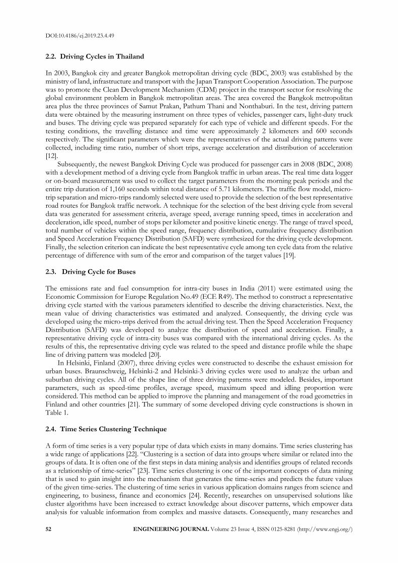
2.2. Driving Cycles in Thailand In 2003, Bangkok city and greater Bangkok metropolitan driving cycle (BDC, 2003) was established by the ministry of land, infrastructure and transport with the Japan Transport Cooperation Association. The purpose was to promote the Clean Development Mechanism (CDM) project in the transport sector for resolving the global environment problem in Bangkok metropolitan areas. The area covered the Bangkok metropolitan area plus the three provinces of Samut Prakan, Pathum Thani and Nonthaburi. In the test, driving pattern data were obtained by the measuring instrument on three types of vehicles, passenger cars, light-duty truck and buses. The driving cycle was prepared separately for each type of vehicle and different speeds. For the testing conditions, the travelling distance and time were approximately 2 kilometers and 600 seconds respectively. The significant parameters which were the representatives of the actual driving patterns were collected, including time ratio, number of short trips, average acceleration and distribution of acceleration [12].

Subsequently, the newest Bangkok Driving Cycle was produced for passenger cars in 2008 (BDC, 2008) with a development method of a driving cycle from Bangkok traffic in urban areas. The real time data logger or on-board measurement was used to collect the target parameters from the morning peak periods and the entire trip duration of 1,160 seconds within total distance of 5.71 kilometers. The traffic flow model, micro-trip separation and micro-trips randomly selected were used to provide the selection of the best representative road routes for Bangkok traffic network. A technique for the selection of the best driving cycle from several data was generated for assessment criteria, average speed, average running speed, times in acceleration and deceleration, idle speed, number of stops per kilometer and positive kinetic energy. The range of travel speed, total number of vehicles within the speed range, frequency distribution, cumulative frequency distribution and Speed Acceleration Frequency Distribution (SAFD) were synthesized for the driving cycle development. Finally, the selection criterion can indicate the best representative cycle among ten cycle data from the relative percentage of difference with sum of the error and comparison of the target values [19]. 2.3. Driving Cycle for Buses The emissions rate and fuel consumption for intra-city buses in India (2011) were estimated using the Economic Commission for Europe Regulation No.49 (ECE R49). The method to construct a representative driving cycle started with the various parameters identified to describe the driving characteristics. Next, the mean value of driving characteristics was estimated and analyzed. Consequently, the driving cycle was developed using the micro-trips derived from the actual driving test. Then the Speed Acceleration Frequency Distribution (SAFD) was developed to analyze the distribution of speed and acceleration. Finally, a representative driving cycle of intra-city buses was compared with the international driving cycles. As the results of this, the representative driving cycle was related to the speed and distance profile while the shape line of driving pattern was modeled [20].

In Helsinki, Finland (2007), three driving cycles were constructed to describe the exhaust emission for urban buses. Braunschweig, Helsinki-2 and Helsinki-3 driving cycles were used to analyze the urban and suburban driving cycles. All of the shape line of three driving patterns were modeled. Besides, important parameters, such as speed-time profiles, average speed, maximum speed and idling proportion were considered. This method can be applied to improve the planning and management of the road geometries in Finland and other countries [21]. The summary of some developed driving cycle constructions is shown in Table 1. 2.4. Time Series Clustering Technique A form of time series is a very popular type of data which exists in many domains. Time series clustering has a wide range of applications [22]. “Clustering is a section of data into groups where similar or related into the groups of data. It is often one of the first steps in data mining analysis and identifies groups of related records as a relationship of time-series” [23]. Time series clustering is one of the important concepts of data mining that is used to gain insight into the mechanism that generates the time-series and predicts the future values of the given time-series. The clustering of time series in various application domains ranges from science and engineering, to business, finance and economics [24]. Recently, researches on unsupervised solutions like cluster algorithms have been increased to extract knowledge about discover patterns, which empower data analysis for valuable information from complex and massive datasets. Consequently, many researches and

DOI:10.4186/ej.2019.23.4.49


projects have been performed with different objectives, such as subsequence matching, anomaly detection, motif discovery, indexing, clustering classification, visualization, segmentation, identify patterns, trend analysis and forecasting [25].

Previously, the development of a time series clustering algorithm was classified into three major categories raw-data-based, feature-based and model-based methods. The raw-data-based method concentrates, on raw data either in the time or frequency domain. Two-time series being compared are normally sampled at the same interval, but their lengths or number of the time points might or might not be the same. This category is able to apply several clustering algorithms including K-means and Fuzzy c-means. Clustering algorithm on raw-data based method is desirable to deal with high dimensional space especially in fast sampling rate. But it was also unsatisfactory to work directly on the raw and highly noisy data. Hence, several feature-based clustering methods have been concerned to replace the previous method. For the model-based clustering method, the determination of each time series is produced by a mixture of underlying probability distributions [26]. However, existing clustering algorithms were weak in extracting smooth subspaces for clustering time series data. A new k-means types with smooth subspaces named Time Series k- means (TSkmeans) was developed. Specifically, the smooth subspaces were presented by weighted time stamp which indicated the relation of these time stamps for clustering objects. This method was applied in terms of common performance metrics, such as accuracy, Fscore, RandIndex and normal mutual information [27]. Similarly, the pseudo-metrics use the large sample size with the nearest neighbor classification [28]. Therefore, most of time series clustering algorithm related to works can be categorized into three types, whole time series clustering, subsequence time series clustering and time point clustering. The characteristics of the three categories time series clustering are shown in Fig. 1. The whole time series clustering is considered as clustering of overall data. While the subsequence time series clustering is determined for some segments from a long time series or some parts of whole time. For the time point clustering, grouping the time point based on a combination of their temporal proximity of time points and the similarity of the corresponding values or trends is considered [25].

Fig. 1. Characteristics of time series clustering.

DOI:10.4186/ej.2019.23.4.49


Table 1. Summaries of some developed cycle construction.

Driving cycle Category/

Driving Pattern Data collection Significant parameters Assessment criteria

Total time duration (s)/ Total distance (m)

New European Driving Cycle (NEDC)

Standard Driving Cycle/ Polygonal

On-board measurement

Average speed

Average acceleration/deceleration

Average number of acceleration/deceleration changes

Mean length of micro-trip

Traffic Flow Index Method (TRAFIX)

Absolute value of the relative error of speeds

UDC 780/3,976 EUDC 400/6,956 Combined

1,180/10,932

Federal Test Procedure (FTP-75)

Standard Driving Cycle/ Modal


Average speed

Number of stop per distance

Maximum speed

Speed Acceleration Frequency Distribution

Speed codes

43% cold, 53% hot

Urban Dynamometer Driving Schedule 505/12,070

The City 1,369/5,780 Combined

1,874/17,770

Bangkok City and Greater Bangkok Metropolitan (BDC, 2003)

Realistic Driving Cycle/ Polygonal


4-mode time ratio

Number of short trip

Average acceleration

Distribution of acceleration

Vehicle speed distribution

Distribution of frequency

Ratio of idle time

600 or more/2,000

Bangkok Driving Cycle (BDC, 2008)

Realistic Driving Cycle/

Modal


Average speed

Average running speed

Times in acceleration and deceleration

Idle speed

Number of stops per kilometer

Positive kinetic energy

Range of travel speed

Total number of vehicle within the speed range

Frequency distribution

Cumulative frequency distribution


1,160/5,710

DOI:10.4186/ej.2019.23.4.49


Table 1. Summaries of some developed cycle construction [Cont.].

Driving cycle Category/ Driving Pattern

Data collection Significant parameters Assessment criteria Total time duration (s)/ Total distance (m)

Singapore Driving Cycle (SDC, 2014)

Realistic Driving Cycle/Modal


Average speed of the entire trip


Average micro-trip duration

Average acceleration of all acceleration/ deceleration phases

Average number of stops per kilometer

Average number of acceleration/ deceleration changes

Percentage of driving mode idling/ cruising/acceleration/deceleration/ creeping

Maximum speed/acceleration/ deceleration

Minimum acceleration/deceleration


Comparison with New European Driving Cycle

2,344/21,500

Hong Kong Driving Cycle (HDC, 2007)


On-board measurement and chase car method

Average speed of the entire trips


Average acceleration/deceleration

Average micro-trip duration

Time proportions of driving modes for idling/acceleration/deceleration

Positive kinetic energy

Sum Average Absolute Percentage Error

Sum Square Difference


Speed Acceleration Probability Distributions

Root mean square acceleration

1,500/6,900

ATHENS Driving Cycle (ADC, 2002)



Similar to the New European Driving Cycle (NEDC)

16 phases of various durations

Comparison with New European Driving Cycle

1,180/6,512

DOI:10.4186/ej.2019.23.4.49


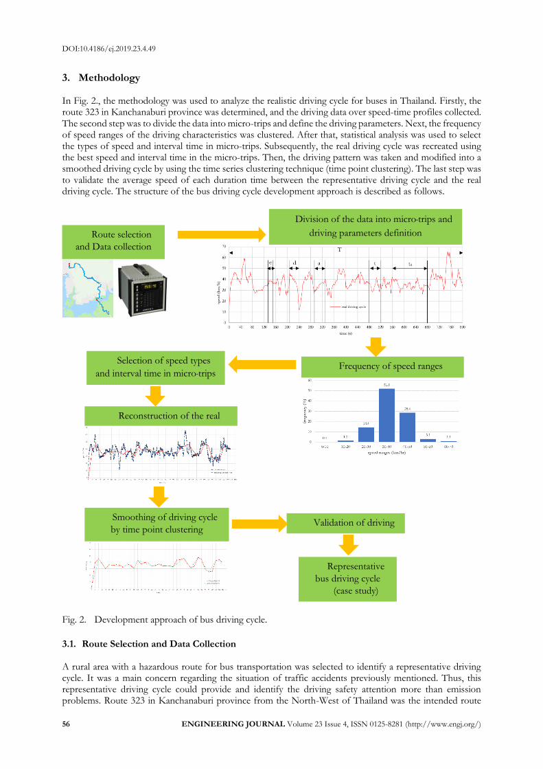
3. Methodology In Fig. 2., the methodology was used to analyze the realistic driving cycle for buses in Thailand. Firstly, the route 323 in Kanchanaburi province was determined, and the driving data over speed-time profiles collected. The second step was to divide the data into micro-trips and define the driving parameters. Next, the frequency of speed ranges of the driving characteristics was clustered. After that, statistical analysis was used to select the types of speed and interval time in micro-trips. Subsequently, the real driving cycle was recreated using the best speed and interval time in the micro-trips. Then, the driving pattern was taken and modified into a smoothed driving cycle by using the time series clustering technique (time point clustering). The last step was to validate the average speed of each duration time between the representative driving cycle and the real driving cycle. The structure of the bus driving cycle development approach is described as follows.

Fig. 2. Development approach of bus driving cycle.

3.1. Route Selection and Data Collection A rural area with a hazardous route for bus transportation was selected to identify a representative driving cycle. It was a main concern regarding the situation of traffic accidents previously mentioned. Thus, this representative driving cycle could provide and identify the driving safety attention more than emission problems. Route 323 in Kanchanaburi province from the North-West of Thailand was the intended route

Division of the data into micro-trips and

driving parameters definition Route selection

and Data collection

Frequency of speed ranges

clustering

Selection of speed types

and interval time in micro-trips

Reconstruction of the real

driving cycle

Smoothing of driving cycle

by time point clustering

technique

Representative

bus driving cycle

(case study)

Validation of driving

cycle

DOI:10.4186/ej.2019.23.4.49


target as shown in Fig. 3. On this route, there are various road factors related to traffic accidents such as slopes of more than 7% gradient, narrow curves and continuous curves with a distance of 3 kilometers. Therefore, this route was suitable for the time clustering technique as a case study. Moreover, it could be applied to improve the quality of buses and other road designs including the driving safety. To collect the driving data, the on-board measurement method using EDX-200A data acquisition was used along the selected route. The main part of instrumentation includes On-board data logger, pedal force, speed and acceleration sensors and Global Positioning System (GPS) that can be recorded every second. Driving data collection was performed under real traffic conditions during the morning peak time within the trip duration of 1,100 seconds and total distance of 11.481 kilometers. 3.2. Driving Data Division Using Time Series Clustering Technique and Driving Parameters

Definition The process of driving data partitioning is based on the definition of micro-trips. “Micro-trip” is a short travel between two continual time points until the vehicle is stopped [29]. Therefore, the related driving characteristics with similarity were identified into clusters as a relationship of time-series [23]. In this study, the time series in the part of motion consists of acceleration (a), deceleration (d), constant speed (c), interval time (t), duration time (td) and total time (T). An example of clustering of typical travelling data is shown in Fig. 4.

To utilize the driving cycle on chassis dynamometer, further work on the test procedure should be conducted. The representative driving cycle was developed using the time series clustering technique. The time series clustering technique especially with time point in raw-data-based method was a fundamental process to construct the representative driving cycle.

Fig. 3. Chosen route for collection of driving data (Route 323 in Kanchanaburi province, North-West

Thailand): (Adapted from Google Maps).

DOI:10.4186/ej.2019.23.4.49


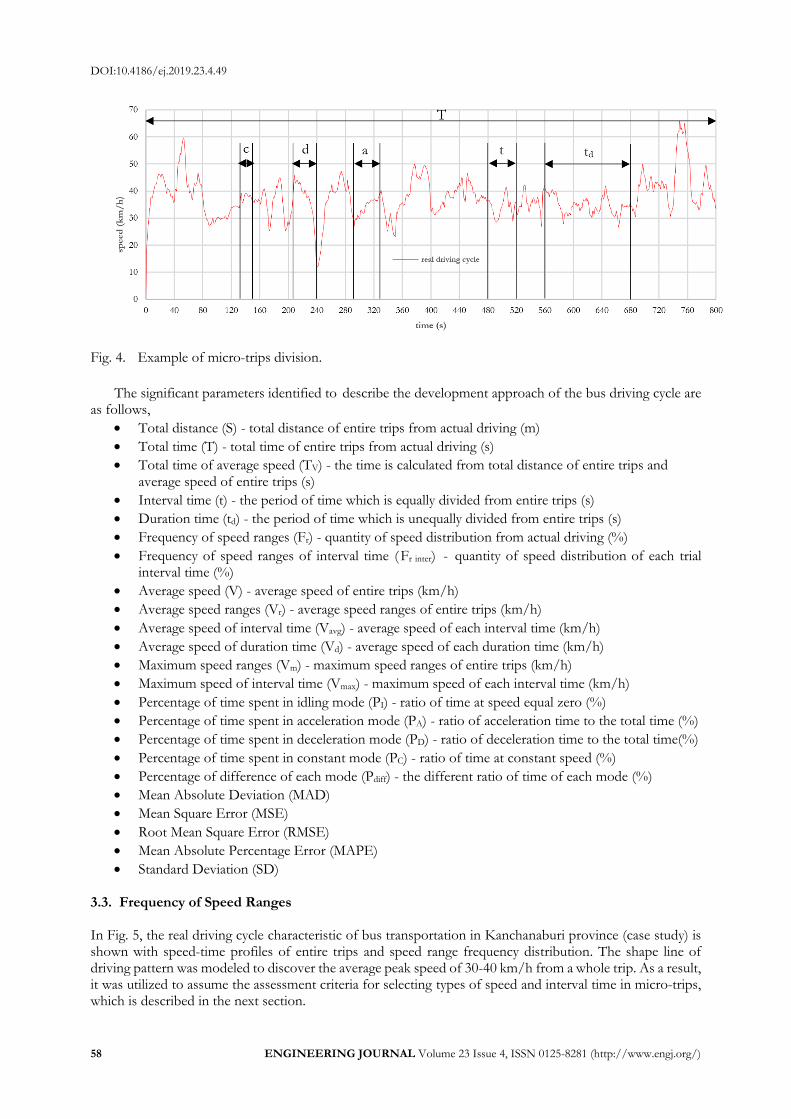
Fig. 4. Example of micro-trips division.

The significant parameters identified to describe the development approach of the bus driving cycle are as follows,

Total distance (S) - total distance of entire trips from actual driving (m)

Total time (T) - total time of entire trips from actual driving (s)

Total time of average speed (TV) - the time is calculated from total distance of entire trips and average speed of entire trips (s)

Interval time (t) - the period of time which is equally divided from entire trips (s)

Duration time (td) - the period of time which is unequally divided from entire trips (s)

Frequency of speed ranges (Fr) - quantity of speed distribution from actual driving (%)

Frequency of speed ranges of interval time (Fr inter) - quantity of speed distribution of each trial interval time (%)

Average speed (V) - average speed of entire trips (km/h)

Average speed ranges (Vr) - average speed ranges of entire trips (km/h)

Average speed of interval time (Vavg) - average speed of each interval time (km/h)

Average speed of duration time (Vd) - average speed of each duration time (km/h)

Maximum speed ranges (Vm) - maximum speed ranges of entire trips (km/h)

Maximum speed of interval time (Vmax) - maximum speed of each interval time (km/h)

Percentage of time spent in idling mode (PI) - ratio of time at speed equal zero (%)

Percentage of time spent in acceleration mode (PA) - ratio of acceleration time to the total time (%)

Percentage of time spent in deceleration mode (PD) - ratio of deceleration time to the total time(%)

Percentage of time spent in constant mode (PC) - ratio of time at constant speed (%)

Percentage of difference of each mode (Pdiff) - the different ratio of time of each mode (%)

Mean Absolute Deviation (MAD)

Mean Square Error (MSE)

Root Mean Square Error (RMSE)

Mean Absolute Percentage Error (MAPE)

Standard Deviation (SD) 3.3. Frequency of Speed Ranges In Fig. 5, the real driving cycle characteristic of bus transportation in Kanchanaburi province (case study) is shown with speed-time profiles of entire trips and speed range frequency distribution. The shape line of driving pattern was modeled to discover the average peak speed of 30-40 km/h from a whole trip. As a result, it was utilized to assume the assessment criteria for selecting types of speed and interval time in micro-trips, which is described in the next section.

DOI:10.4186/ej.2019.23.4.49


(a) speed-time profiles of entire trips

(b) speed range frequency distribution

Fig. 5. Real driving cycle characteristics of bus on target route.

3.4. Selection of Speed Types and Interval Time in Micro-Trips In this section, the results of speed range frequency distribution and statistical analysis were used to select the types of speed and interval time in micro-trips. The speed-time profile characteristics are the key point of driving cycle construction. It does not appropriately reveal the type of speed (maximum or average) and the interval time separations to closely reflect the actual driving. For this reason, it is necessary to investigate the driving cycle with different types of speed and different interval time separations. To aid understanding, the selection of speed types and interval time are described step-by-step below and the results shown in Table 2.

Step 1. Take the peak of frequency of speed ranges (Fr) from actual driving to the assumption. In this case, the peak appeared as 51.8% at speed range of 30-40 km/h.

Step 2. Calculate the average speed of entire trips (V) and total time of average speed (TV) using Eq. (1) and Eq. (2) respectively. This method is found in the New European Driving Cycle (NEDC).

Step 3. Use the difference between total time of average speed (TV) and total time of entire trips from actual driving time (T) to identify the interval time (t) using Eq. (3).

Step 4. Trial five interval times starting from an initial valve of calculation result in Eq. (3) as “trial 1, 2, 3, 4 and 5”. For instance, the interval time was equally calculated from the initial value of 20 s. Therefore, five trials of interval times are trial 1 (t = 20 s), trial 2 (t = 25 s)….trial 5 (t = 40 s) (see Table 2).

DOI:10.4186/ej.2019.23.4.49


Step 5. Count the quantity of speed distribution between maximum speed (Vmax) and average speed (Vavg) at speed ranges 30-40 km/h. of each trial interval time. (see Table 3).

Step 6. Select a suitable type of speed by the quantity of speed distribution of trial interval time that

can be more than or equal to actual driving (Fr inter Fr) due to the threshold in this study (see Table 3).

Step 7. Analyze all of trial interval times against the chosen type of speed using statistical analysis including Mean Absolute Deviation (MAD), Mean Square Error (MSE), Root Mean Square Error (RMSE), Mean Absolute Percentage Error (MAPE) and Standard Deviation (SD). Then, the lowest value from statistical analysis is chosen (see Table 4). In this study, the best trial interval time was prepared for driving cycle reconstruction and referred to as “candidate driving cycle”,

where,

Average speed of entire trips 𝑉 =S

𝑇 (1)

Total time of average speed 𝑇𝑉 =S

𝑉 (2)

Interval time 𝑡 = |𝑇𝑉 − 𝑇| (3)

Table 2. Actual driving information and interval time calculation.

Actual driving information Interval time calculation

Speed ranges (km/h)

Fr (%)

Vr (km/h)

T (s)

S (m)

V (km/h)

TV (s)

t (s)

0-10 0.1 0.0

1,100 11,481 36.9 1,120 20

10-20 1.2 15.8

20-30 14.4 27.0

30-40 51.8 35.1

40-50 28.4 43.8

50-60 3.1 53.7

60-70 1.1 62.6

Table 3. Type of speed versus frequency of speed ranges of each trial interval time.

Type of speed

Frequency of speed range @ 30-40 km/h of each trial interval time (Fr inter)

trial 1 (t= 20 s)

trial 2 (t= 25 s)

trial 3 (t= 30 s)

trial 4 (t= 35 s)

trial 5 (t= 40 s)

Vmax 32.1 % 26.7 % 18.9 % 12.1 % 17.2 %

Vavg 57.1 % 57.8 % 64.9 % 66.7 % 65.5 %

Table 4. Statistical analysis for selection of the best interval time.

Type of speed Interval time (s) Statistical analysis

MAD MSE RMSE MAPE SD

Vavg

trial 1 (t = 20 s) 0.370 7.531 2.774 1.010 6.725

trial 2 (t = 25 s) 0.667 19.567 4.424 1.769 7.223

trial 3 (t = 30 s) 0.430 6.832 2.614 1.146 7.092

trial 4 (t = 35 s) 0.892 25.45 5.045 2.464 6.750

trial 5 (t = 40 s) 0.111 0.344 0.587 0.030 6.567

As the result of the driving information in Table 2, the total time of average speed (TV) was recalculated

and changed from the existing total time (T) as 1,100 seconds to 1,120 seconds with interval time of 20 seconds. Besides, the speed range of 30-40 km/h was used to select the type of speed as shown in Table 3.

DOI:10.4186/ej.2019.23.4.49


Regarding the maximum speed (Vmax) in Table 3, the frequency of speed distribution of each interval time was less than the assessment criterion. Hence, the selected type of speed was average speed (Vavg), since Fr

inter 51.8%. Consequently, the best trial interval time was decided by using statistical analysis. From Table 4, it was found that the least value from statistical analysis was in trial 5 (t = 40 s). Therefore, average speed (Vavg) and interval time (t = 40 s) were chosen in this case study. In other words, it was an appropriate decision to reflect the actual driving. Thus, the driving cycle is reconstructed and described in the next section. 3.5. Reconstructed Driving Cycle In the previous section, a suitable type of speed and the best interval time were estimated to recreate the driving cycle. This driving cycle is called “candidate driving cycle”. In the beginning of the reconstructed candidate driving cycle, the interval time was separated equally by 40 seconds (t = 40 s) and the average grouped speeds of each interval time were identified through subsequence clustering segments. Then, the type of shape line was made by a scatter plot with straight line function to construct the candidate driving cycle. This method can be seen in reference [25]. In Fig. 6, there are different graphs between real driving cycle from each data point and the shape line from the candidate driving cycle. However, the characteristics of both driving cycles are the same because the selection criteria, type of speed and interval time are used with the consideration of subsequence clustering segments and statistical analysis. 3.6. Representative Driving Cycle To represent the driving cycle for chassis dynamometer testing protocol, similarity or related driving characteristics was firstly identified into clusters as a relationship of time-series [23]. Then, the candidate driving cycle was developed to be the representative driving cycle using time point clustering. This may constitute identifying common trends occurring at different times or similarity in shape. Based on research works from Zhang et al and Liao [22, 26], the duration time is identified from the same trend of the continuous time points in which the interval time might or might not be the same. Therefore, the length of the time points shall not be the same in this research approach. The individual length of the time between beginning point to end point was prescribed to “duration time” and defined in abbreviation as (td). This method is considered to integrate the same trend of speed at each time point with acceleration and deceleration modes. It was also satisfactory to work directly with time point clustering. Developed driving cycle using time series clustering technique (time point clustering) is shown in Fig. 7 and referred to as “representative driving cycle”. From the view point of assessment, the average speed of each duration time between real driving cycle and representative driving cycle was validated by statistical hypothesis test and indicated in Table 5.

Fig. 6. Reconstructed driving cycle.

DOI:10.4186/ej.2019.23.4.49


Fig. 7. Developed candidate driving cycle using time point clustering and referred to as representative

driving cycle.

Table 5 shows the cycle verification with a statistical test between representative driving cycle and real driving cycle. For developing driving cycle verification, the result of a statistical hypothesis test showed that the variation in a data set has low values that changed in the mean absolute error and deviation. This was correlated to the criterion in other driving cycle research. “The developed driving cycle was accepted if the range of differences within 5% to 10%” [16, 19]. “The change in absolute error across all candidate driving cycles and the mean absolute deviation when compared to the target or real cycle” [30]. Therefore, the verification of a representative driving cycle is an important process to assess the suitability of the developed driving cycle. Likewise, the ratio of time of each mode estimation for verification was shown in Table 6. The percentage difference changed by ± 9.19% in acceleration and deceleration modes. Hence, this representative driving cycle can be used as a case study for bus transportation in Thailand because of difference was within 10% based on the developed threshold. Finally, the representative driving cycle concerning bus transportation for Thailand in a case study is shown in Fig. 8.

Fig. 8. Representative driving cycle concerning bus transportation for Thailand in a case study.

DOI:10.4186/ej.2019.23.4.49


Table 5. Driving cycle verification with statistical hypothesis test.

Duration

time (td)

Average speed (km/h) Statistical hypothesis test

Real driving cycle

Representative driving cycle

MAD MSE RMSE MAPE SD

0-80 42.3 37.5

0.269 1.301 1.141 0.732 3.943

80-120 30.1 30.1

120-160 36.4 36.4

160-240 35.6 24.2

240-280 35.4 35.4

280-400 36.7 36.4

400-440 36.4 36.4

440-520 36.7 37.9

520-560 36.0 36.0

560-600 35.4 35.4

600-640 34.1 34.1

640-680 34.1 34.1

680-760 44.6 45.4

760-840 35.6 43.7

840-880 37.7 37.7

880-1000 34.7 39.6

1000-1080 39.2 35.2

1080-1100 40.5 41.2

1100-1120 40.5 41.2

Table 6. Comparison ratio of time of each mode in motion.

Typical driving cycles

Ratio of time of each mode in motion (%) Idling

(PI) Acceleration

(PA) Constant

(PC) Deceleration

(PD)

Real N/A 52.05 1.79 46.16

Representative N/A 42.86 1.79 55.35

Percentage of difference of each

mode (Pdiff) - ±9.19 0.00 ±9.19

4. Conclusions

This study attempted to develop a realistic driving cycle of bus transportation in a rural area using time series clustering technique. This was because the situation of traffic accident can be considered for the driving safety more than the emission control. A representative driving cycle for buses was developed using the second-by-second driving data collected within the trip duration of 1,100 seconds and total distance of 11.481 kilometers. Route 323 in Kanchanaburi province from West-North of Thailand was the intended route target.

The frequency of speed ranges appeared to peak at 30-40 km/h with 51.8%. The results showed that the best solution for the interval time of entire trips was equally 40 seconds with average speed type which is close to the actual driving data. Furthermore, results indicated the variation in a data set of developed driving cycle had low change values in the mean absolute error and deviation. In terms of the ratio of time of each mode estimation, the percentage difference changed by ± 9.19% in acceleration and deceleration modes with higher ratio of time spent in deceleration mode. This is acceptable because of 10% difference based on the developed threshold. Therefore, this technique can be used to construct a driving cycle for other countries

DOI:10.4186/ej.2019.23.4.49


and easily utilized in the chassis dynamometer operation. Hence, using bus transportation in Thailand as a case study, this representative driving cycle provides strong encouragement for driving safety testing protocol.

Acknowledgements

The authors acknowledge the funding for this work by the Department of Land Transport, Thailand, and the helpful support with data collection from the King Mongkut’s University of Technology North Bangkok and Department of Mechanical Engineering, Rajamangala University of Technology Phra Nakhon. We would also like to thank the valuable comments of the reviewers to fulfill this research work.

References

[1] Ministry of Transport, “Transportation Statistic Report,” Transp. Portal, Thailand, 2016.

[2] N. O-Charoen, “Pubilc bus service quality and safety evaluation,” Tha. Transp. and Logistics Policy,

Bangkok, Thailand, 2016.

[3] Bureau of Highway Safety, “101 danger routes 60,” Dept. of HWY, Thailand, 2017.

[4] Royal Thai Police, “The situation of traffic accident cause of the accident by a person and environment

causes of the equipment used in driving, Whole Kingdom: 2006-2015,” R. Tha. Police, Thailand, 2015.

[5] P. Vinichi, “Problem and obstacles of police officers in implementing traffic accident prevention policy

in Chiang Mai Province during the New Year Festival 2013,” M.S. thesis, Graduate School, Chiang Mai

University, Thailand, 2013.

[6] World Health Organization, “Global Status Report on Road Safety 2015,” WHO, Geneva, Switzerland,

2015.

[7] M. Abe, “Vehicle dynamics and control,” in Vehicle Handling Dynamics, 2nd ed. Japan: Elsevier, 2015, p.

48.

[8] I. Dukulis and V. Pirs, “Development of driving cycles for dynamometer control software coresponding

to peculilarities of Latvia,” in Proceedings of the 15th International Scientific Conference, Jelgava, Latvia, 2009,

pp. 95-102.

[9] D. Huang, H. Xie, H. Ma, and Q. Sun, “Driving cycle prediction model based on bus route features”

Transp. Res. Part D, Transp. and Environ., vol. 54, pp. 99-113, Jul. 2017.

[10] S. Tamasanya, S. Chungpaibulpatana, and S. Atthajariyakul, “Development of automobile Bangkok

Driving Cycle for emissions and fuel consumption assessment,” in the 2nd Joint International Conference on

Sustainable Energy and Environment (SEE 2006), Thailand, 2006, pp. 1-6.

[11] The United Nations Economic Commission for Europe (UNECE), Braking Tests and Performance of

Braking Systems Regulation 13. Sep. 2004.

[12] Ministry of Land, Infrastructure and Transport, “Study to promote CDM project in transport sector in

order to resolve global environment problem (Bangkok metropolitan area case),” Jpn. Transp. Coop.

Assoc., Thailand, Nov. 2004.

[13] B. Freij and E. Ericsson, “Influence of street characteristics, driver category and car performance on

urban driving patterns,” Transp. Res. Part D, Transp. and Environ., vol. 10, no. 3, pp. 213-229, May 2005.

[14] J. Kuhlwein, J. German, and B. Anup, “Development of test cycle conversion factors among worldwide light-duty vehicle CO2 Emission standard,” Council on Clean Trans, Washington DC, 2004

[15] E. Tzirakis, K. Pitsas, F. Zannikos, and S. Stournas, “Vehicle emissions and driving cycle: comparison

of the Athens Driving Cycle (ADC) with ECE-15 and European Driving Cycle (EDC),” Glob. NEST

J., vol. 8, no. 3, pp. 282-290, Nov. 2006.

[16] H. Y. Tong, W. T. Hung, and C. S. Cheung, “Development of a driving cycle for Hong Kong,” Atmos.

Environ. J., vol. 33, no. 15, pp. 2323-2335, Jan. 1999.

[17] W. T. Hung, H. Y. Tong, C. P. Lee, K. Ha, and L. Y. Pao, “Development of a practical driving cycle

construction methodology: A case study in Hong Kong,” Transp. Res. Part D, Transp. and Environ., vol.

12, no. 2, pp. 115-128, Mar. 2007.

[18] S. H. Ho, Y. D. Wong, and V. W. Chang, “Developing Singapore Driving Cycle for passenger cars to

estimate fuel consumption and vehicular emissions,” Atmos. Environ. J., vol. 97, pp. 353-362, Nov. 2014.

DOI:10.4186/ej.2019.23.4.49


[19] S. Tamasanya, S. Chungpaibulpatana, and B. Limmeechokchai, “Development of a driving cycle for the

measurement of fuel consumption and exhaust emission of automobiles in Bangkok during peak

periods,” Int. J. Aut. Technol., vol. 10, no. 2, pp. 251-264, 2009.

[20] K. S. Nesamani and K. P. Subramanian, “Development of a driving cycle for intra-city buses in Chennai,

India,” Atmos. Environ. J., vol. 31 no. 45, pp. 5469-5476, Oct. 2011.

[21] N. O. Nylund, K. Erkkilä, and T. Hartikka, “Fuel consumption and exhaust emissions of urban buses,”

VTT Tech. Res. Cent. of Finl., Finland, 2007.

[22] X. Zhang, J. Liu, Y. Du, and L. Ting, “A novel clustering method on time series data,” Expert. Syst. Appl.

J., vol. 38, no. 9, pp. 11891-11900, Sep. 2011.

[23] P. Rai and S. Singh, “A Survey of clustering techniques,” Int. J.Com. Appl., vol. 7, no. 12, pp. 975-8887,

Oct. 2010.

[24] S. Rani and G. Sikka, “Recent techniques of clustering of time series data,” Int. J.Com. Appl., vol. 52, no.

15, pp. 975-8887, Aug. 2012.

[25] S. Aghabozorgi, A. S. Shirkhorshidi, and T. Y. Wah, “Time-series clustering - A decade review,” Inf. Syst.

J., vol. 53, pp. 16-38, Oct.-Nov. 2015.

[26] T. W. Liao, “Clustering of time series data-a survey,” Pattern Recognit. J., vol. 38, no. 11, pp. 1857-1874,

Nov. 2005.

[27] X. Huang, Y. Ye, L. Xiong, Y. K. Lau, N. Jiang, and S. Wang, “Time series k -means: A new k -means

type smooth subspace clustering for time series data,” Inf. Sci. J., vol. 367-368, pp. 1-13, 2016.

[28] T. Korsrilabutr and B. Kijsirikul, “Pseudometrics for nearest neighbor classification of time series data,”

Engineering Journal, vol. 13, no. 2, pp. 19-42, 2009.

[29] A. Fotouhi and M. Montazeri-Gh, ‘‘Tehran driving cycle development using the k-means clustering

method,’’ Transp. A, Civil Eng., vol. 20, no. 2, pp. 286-293, Oct. 2012.

[30] D. J. Bishop, C. J. Axon, and M. D. Culloch, “A robust, data-driven methodology for real-world driving

cycle development,” Transp. Res. Part D, Transp. and Environ., vol. 17, no. 5, pp. 389-397, Jul. 2012.

driving cycle using time series clustering technique for

Documents