Drilling and Testing the DOI­04­1A Coalbed Methane Well, Fort Yukon, Alaska 

By Arthur Clark, Charles E. Barker, and Edwin P. Weeks 

 

       

Open-File Report 2009-1064 U.S. Department of the Interior U.S. Geological Survey 

U.S. Department of the Interior KEN SALAZAR, Secretary U.S. Geological Survey Suzette M. Kimball, Acting Director U.S. Geological Survey, Reston, Virginia: 2009 For product and ordering information: World Wide Web: http://www.usgs.gov/ Telephone: 1-888-ASK-USGS For more information on the USGS – the Federal source for science about the Earth, its natural and living resources, natural hazards, and the environment: World Wide Web: http://www.usgs.gov Telephone: 1-888-ASK-USGS Suggested citation: Clark, A., Barker, C.E., and Weeks, E.P. 2009, Drilling and testing the DOI-04-1A coalbed methane well, Fort Yukon, Alaska: U.S. Geological Survey Open-File Report 2009–1064, 69 p. Any use of trade, product, or firm names is for descriptive purposes only and does not imply endorsement by the U.S. Government. Although this report is in the public domain, permission must be secured from the individual copyright owners to reproduce any copyrighted material contained within this report.

ii

Contents Introduction…………………………………………………………………………………………...…1

Background…………………………………………………………………………………….…...2 Project Objectives………………………………………………………………………………….4 Acknowledgements………………………………………………………………………………...5 References…………………………………………………………………………………...…..…6

Section 1: Drilling and Testing Overview……………………………………………………………7 Introduction……………………………………………………………………………………….…7 Equipment…………………………………………………………………………………...…..….8 Equipment Transport……………………………………………………………………..….....…8 Drilling Operations…………………………………………………………………………..…..…9 Geophysical Logging…………………………………………………………………….........…14 Monitor Well Installation………………………………………………………………...…….…17 Well Development and Testing…………………………………………………………........…18 Spring 2005 Activities…………………………………………………………...………….……20 Results…………………………………………………………...…………………………..……22

Section 2: Canister Desorption Results………………………………………………………..…..25 Introduction………………………………………………………………...................................25 Desorption Technique………………………………………………………………..…………..28 Lost-Gas Estimate…………………………………………………………..………………...….28 Sampling Desorbed Gas…………………………………………………………..……….……29 Analysis of Desorption Data………………………………………………….………….………30 Coring Operations……………………………………………………………….…………..……30 Results………………………………………………………………….………………………….31 Desorption………………………………………………….………………………………...……31 Coal Quality………………………………………………………………..……………...………31 Desorbed Gas Analyses………………………………………………………….………...……32 Coalbed Saturation from Isotherms…………………………………………………………….33 References…………………………………………………………….………………………..…36

Section 3: Aquifer Test and Water Quality Analyses…………………………………..…………43 Introduction……………………………………………………….…………………….…………43 Hydrogeologic Setting……………………………………………………………….……...……47 Well Completion and Initial Development………………………………………………..…….48 Well Tests and Slug Test Theory…………………………………………………….…………49 Test 1……………………………………………………………………….………………...……51 Events Leading to Test 2……………………………………………………………………...…55 Test 2………………………………………………………………………………………....……56 Events Leading to Test 3…………………………………………………………………..…….56 Test 3………………………………………………………………………………….……...……57 Winter Data……………………………………………………………………………………..…58 Test 4………………………………………………………………………………………………61 Summary of Aquifer Test Analyses…………………………………………………..…………61 Water Chemistry Analyses………………………………………………………………………62 References…………………………………………………………………….…….…….………66

Summary of Results……………………………………………………………………..……………67 Fort Yukon Production Potential……………………………………………………...…………67 References………………………………………………………………………………...………69

iii

iv

Figures 1. Map of Alaska showing location of Yukon Flats Basin and Fort Yukon………………….…2 1-1. Photograph of drill rig at Fort Yukon CBM drill site DOI-04-1A………………………….…10 1-2. Generalized lithology of borehole DOI-04-1A………………………………………………..13 1-3. Photograph of geophysical logging winch and operating system………………………….14 1-4. Geophysical logs of drill hole DOI-04-1A……………………………………………..………16 1-5. Configuration of monitor well DOI-04-1A…………………………………………...……...…19 1-6. Photograph of Fort Yukon drill site………………………………………………….…………20 1-7. Temperature log for well DOI-04-1A………………………………………………………..…21 2-1. Geophysical logs of drill hole DOI-04-1A…………………………………………….……….27 2-2. Methane adsorption isotherm for canister 104-5…………………………………..……...…34 2-3. Methane adsorption isotherm for canister 104-33…………………………………..….……35 2-4. Temperature log for well DOI-04-1A……………………………………………………...…...36 3-1. Geologic profile and configuration of DOI-04-1A CBM well…………………………………48 3-2A. Data plots………………………………………………………………………………...………53 3-2B. Data plots…………………………………………………………………………………...……54 3-3. Graph of pressure head vs. time……………………………………………………....………60 3-4. Piper Diagram comparing water samples, drill hole DOI-04-1A……………………....……65

Tables 2-1A. Summary of canister desorption results, upper coal zone………………………….………39 2-1B. Summary of canister desorption results, lower coal zone……………………………..……40 2-2A. Summary of proximate and specific gravity analysis, upper coal zone……………………41 2-2B. Summary of proximate and specific gravity analysis, lower coal zone……………………42 3-1A. Summary of canister desorption results, upper coal zone……………………….…………45 3-1B. Summary of canister desorpton results, lower coal zone………………………………...…46 3-2. Water-level recovery following evacuation to 500-ft depth…………………………………52 3-3. Results of slug-test type curve analyses…………………………………………..…………52 3-4A. Concentrations of major ions in water samples, drill hole DOI-04-1A…………..…………64 3-4B. Concentrations of selected trace elements, drill hole DOI-04-1A………………………….64

Drilling and Testing the DOI-04-1A Coalbed Methane Well, Fort Yukon, Alaska By Arthur Clark1, Charles E. Barker2, and Edwin P. Weeks3

Introduction

The need for affordable energy sources is acute in rural communities of Alaska where

costly diesel fuel must be delivered by barge or plane for power generation. Additionally, the

transport, transfer, and storage of fuel pose great difficulty in these regions. Although small-

scale energy development in remote Arctic locations presents unique challenges, identifying

and developing economic, local sources of energy remains a high priority for state and local

government.

Many areas in rural Alaska contain widespread coal resources that may contain

significant amounts of coalbed methane (CBM) that, when extracted, could be used for power

generation. However, in many of these areas, little is known concerning the properties that

control CBM occurrence and production, including coal bed geometry, coalbed gas content and

saturation, reservoir permeability and pressure, and water chemistry. Therefore, drilling and

testing to collect these data are required to accurately assess the viability of CBM as a potential

energy source in most locations.

In 2004, the U.S. Geological Survey (USGS) and Bureau of Land Management (BLM), in

___________________________________________________________________________

1 U.S. Geological Survey, Denver, Colo. phone: (303) 236-5793 aclark@usgs.gov 2 Scientist Emeritus, U.S. Geological Survey, Denver, Colo. 3 U.S. Geological Survey, Denver, Colo. phone: (303) 236-4981

cooperation with the U.S. Department of Energy (DOE), the Alaska Department of Geological

and Geophysical Surveys (DGGS), the University of Alaska Fairbanks (UAF), the Doyon Native

Corporation, and the village of Fort Yukon, organized and funded the drilling of a well at Fort

Yukon, Alaska to test coal beds for CBM developmental potential. Fort Yukon is a town of about

600 people and is composed mostly of Gwich'in Athabascan Native Americans. It is located

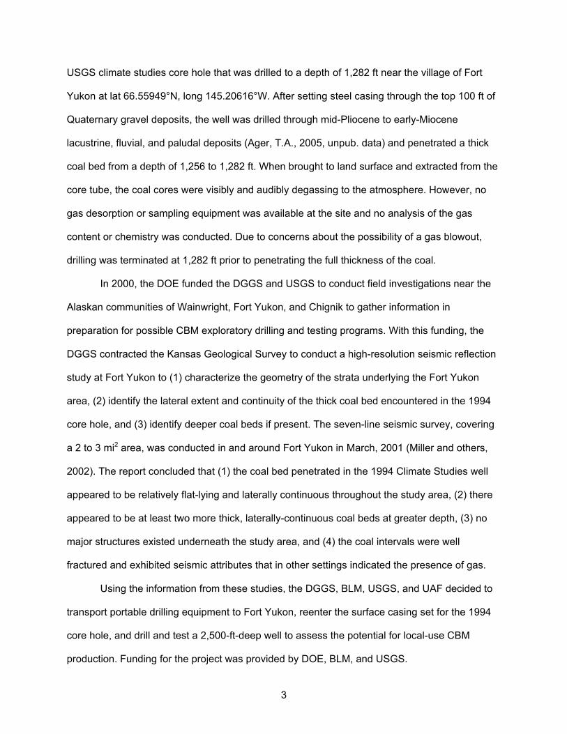
near the center of the Yukon Flats Basin, approximately 145 mi northeast of Fairbanks (fig.1).

Figure 1. Map of Alaska showing location of Yukon Flats basin and Fort Yukon.

Background

The Yukon Flats basin in east-central Alaska is a 8,500 mi2 basin containing up to

10,000 ft of Cenozoic fill including upper Miocene to upper Oligocene nonmarine coal-bearing

lacustrine strata (Kirschner, 1994). CBM potential in the basin was primarily based on a 1994

2

USGS climate studies core hole that was drilled to a depth of 1,282 ft near the village of Fort

Yukon at lat 66.55949°N, long 145.20616°W. After setting steel casing through the top 100 ft of

Quaternary gravel deposits, the well was drilled through mid-Pliocene to early-Miocene

lacustrine, fluvial, and paludal deposits (Ager, T.A., 2005, unpub. data) and penetrated a thick

coal bed from a depth of 1,256 to 1,282 ft. When brought to land surface and extracted from the

core tube, the coal cores were visibly and audibly degassing to the atmosphere. However, no

gas desorption or sampling equipment was available at the site and no analysis of the gas

content or chemistry was conducted. Due to concerns about the possibility of a gas blowout,

drilling was terminated at 1,282 ft prior to penetrating the full thickness of the coal.

In 2000, the DOE funded the DGGS and USGS to conduct field investigations near the

Alaskan communities of Wainwright, Fort Yukon, and Chignik to gather information in

preparation for possible CBM exploratory drilling and testing programs. With this funding, the

DGGS contracted the Kansas Geological Survey to conduct a high-resolution seismic reflection

study at Fort Yukon to (1) characterize the geometry of the strata underlying the Fort Yukon

area, (2) identify the lateral extent and continuity of the thick coal bed encountered in the 1994

core hole, and (3) identify deeper coal beds if present. The seven-line seismic survey, covering

a 2 to 3 mi2 area, was conducted in and around Fort Yukon in March, 2001 (Miller and others,

2002). The report concluded that (1) the coal bed penetrated in the 1994 Climate Studies well

appeared to be relatively flat-lying and laterally continuous throughout the study area, (2) there

appeared to be at least two more thick, laterally-continuous coal beds at greater depth, (3) no

major structures existed underneath the study area, and (4) the coal intervals were well

fractured and exhibited seismic attributes that in other settings indicated the presence of gas.

Using the information from these studies, the DGGS, BLM, USGS, and UAF decided to

transport portable drilling equipment to Fort Yukon, reenter the surface casing set for the 1994

core hole, and drill and test a 2,500-ft-deep well to assess the potential for local-use CBM

production. Funding for the project was provided by DOE, BLM, and USGS.

3

Project Objectives

Due to the remote nature of many of Alaska’s rural communities, with few exceptions,

there are little geologic, hydrologic, or chemical data available when evaluating an area’s

potential for local-use CBM production. Communities located in coal-bearing basins are often a

dozen or more miles away from the closest coal outcrop making it conjectural as to the depth to,

and thickness of, possible coal deposits. In addition, essential reservoir properties such as

hydraulic conductivity and water chemistry, which can only be determined through drilling and

testing programs, are generally not known. Given this dearth of information, the primary

objectives of the 2004 Fort Yukon drilling effort were to (1) determine if lightweight, portable

drilling equipment could be used to effectively and economically collect the data needed to

evaluate an area’s potential for local-use CBM production, (2) collect site-specific data that

would allow an assessment of the CBM potential at Fort Yukon to be made, and (3) gain

knowledge and experience that could be applied to future CBM drilling and testing programs

conducted throughout rural Alaska and in other remote locations.

This report presents the findings of the 2004 drilling program. Section 1 provides a

general overview of project activities including the equipment and procedures used, a project

timeline, and difficulties and problems encountered. Section 2 discusses sampling techniques

and presents canister desorption, reservoir saturation, coal chemistry, and desorbed gas data.

Section 3 provides results of hydraulic testing. Although substantial difficulties were

encountered during aquifer testing procedures, the results of each test are analyzed and

summarized to as great an extent as possible. In addition, this section provides a brief

discussion concerning the chemistry of water samples collected during project operations. The

Summary of Results section uses the collected data to draw preliminary conclusions as to the

potential of local-use CBM production at Fort Yukon.

4

Acknowledgments

Drilling, coring, geophysical logging, hydrologic testing, coal desorption, and other

operations at Fort Yukon were conducted by a consortium consisting of the USGS Central

Energy Resources Team (CERT), the USGS Central Region Research Drilling Project

(CRRDP), the USGS Water Resources Division National Research Program (NRP), the BLM,

the DGGS, and the UAF. The research team consisted of Arthur Clark, Charles Barker and

Steve Roberts of the CERT, Edwin Weeks and Barbara Corland of the NRP, Bob Fisk and Beth

Maclean of the BLM, Jim Clough and Karen Clautice of the DGGS, and David Ogbe and Amy

Rodman of the UAF. Thanks to Fred Grub and Peter Galanis of the USGS in Menlo Park, Calif.

for running the borehole temperature logs in May 2005. Special thanks go to the USGS drill

crew personnel consisting of Jeff Eman, Rob Hunley, Steve Grant, Mike Williams, Mike Schulz,

Thane Bird, and Andrew Ratliff for their hard work and effort, without which the project could not

have been accomplished.

Many thanks are owed to the community of Fort Yukon for the help and cooperation

provided during the project with particular appreciation extended to Fannie Carrol (Fort Yukon

City Manager), Vickie Thomas (Fort Yukon Mayor), James Kelley (Gwitchya Zhee Corporation),

Davey James (Gwitchya Gwich’in Tribal Government) and Bonnie Thomas (Council of

Athabascan Tribal Governments). Special thanks is extended to David Lee Thomas (Gwitchya

Zhee Utility Company) for the expert and enthusiastic assistance provided throughout the

project. Thanks also to Jim Merry and Norm Phillips of the Doyon Corporation for their

assistance and support. The U.S. Air Force 611 CER/CERR at Elmendorf AFB in Anchorage

helped facilitate permitting and logistical requirements and the members of the U.S. Air Force

Fort Yukon Long Range Radar Site provided support throughout. Their help was invaluable and

greatly appreciated.

5

6

References

Kirschner, C.E., 1994, Interior basins of Alaska, in Plafker, G., and Berg, H.C., eds., The

Geology of Alaska, The Geology of North America, v. G-1, Geological Society of America,

p. 469–493.

Miller, R.D., Davis, J.C., Olea, Ricardo, Tapie, Christian, Laflen, D.R., and Fiedler, Mitchell,

2002, Delineation of coalbed methane prospects using high-resolution seismic reflections

at Fort Yukon, Alaska: Kansas Geological Survey, Lawrence, Kansas, Open-File Report

2002-16, 47 p.

Section 1: Drilling and Testing Overview of the DOI-04-1A Coalbed Methane Well, Fort Yukon, Alaska

By Arthur Clark1

Introduction

In the spring of 2004, the Alaska Department of Geological and Geophysical Sciences

(DGGS), using funds from the U.S. Bureau of Land Management (BLM), and working with the

U.S. Geological Survey (USGS), purchased an Atlas Copco-Christensen CS-1000 P6LTM drilling

rig and accessories, 3,000 ft of Atlas Copco-Christensen lightweight HCTTM wireline core rods,

and a hydraulically-powered 35 gallon per minute (gpm) triplex mud-pump to conduct coalbed

methane (CBM) test drilling at selected rural Alaska villages as part of the cooperative Alaska

Rural Energy Project. The equipment, along with other drilling equipment owned and operated

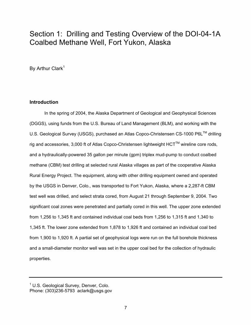
by the USGS in Denver, Colo., was transported to Fort Yukon, Alaska, where a 2,287-ft CBM

test well was drilled, and select strata cored, from August 21 through September 9, 2004. Two

significant coal zones were penetrated and partially cored in this well. The upper zone extended

from 1,256 to 1,345 ft and contained individual coal beds from 1,256 to 1,315 ft and 1,340 to

1,345 ft. The lower zone extended from 1,878 to 1,926 ft and contained an individual coal bed

from 1,900 to 1,920 ft. A partial set of geophysical logs were run on the full borehole thickness

and a small-diameter monitor well was set in the upper coal bed for the collection of hydraulic

properties.

1 U.S. Geological Survey, Denver, Colo. Phone: (303)236-5793 aclark@usgs.gov

7

Equipment

In addition to the drilling rig, the wireline core rods, and the coring mud-pump, several

transport and supply trailers were purchased specifically for this project. Other USGS-owned

equipment including a large-capacity water truck, a 150 gpm duplex mud-pump, and a 1,000

gallon capacity mud-handling system, was used for drilling operations. Primary equipment

included:

CS-1000 P6L drilling-core rig

HCT wireline core system including core rods, barrels, bits, and accessories

3,200-gallon Autocar water truck

Bean 35 gpm triplex core pump

Gardner-Denver 5 in. x 6 in. 150 gpm duplex mud-pump

1,000-gallon capacity mud recirculation and cleaning system

Pickup truck with welder, torches, fuel tank, and tool boxes

25-ft flatbed supply trailer for transport of core rods, barrels, and accessories

25-ft flatbed trailer for transport of the drill rig

16-ft cargo trailer for transport and storage of tools, equipment, and supplies

Light tower and 6 kW generator-trailer

Washington Rotating Control Heads Inc. non-rotating diverter system

Century Geophysical portable logging system and tools

Equipment Transport

On April 22, 2004, all equipment, with the exception of the drilling rig, was loaded onto

Union Pacific railcars in Denver, Colo. for transport to Seattle, Wash. The drilling rig was

delivered to the USGS on April 20 but needed to be assembled and tested prior to shipment.

After initial testing, the rig was loaded onto a 25-ft flatbed trailer and driven from Denver to the

8

Alaska Railroad Barge Terminal in Seattle, Wash., arriving on May 3, where it was stored with

the rest of the equipment awaiting barge transport to Alaska. All of the equipment was then

transferred to the Alaska Railroad Corporation and loaded on an ocean-going barge for

transport to Whittier, Alaska. At Whittier, the railcars were removed from the barge and

transported by rail to Nenana, Alaska where they were unloaded at the Yutana Barge Lines

facility. Yutana Barge Lines then loaded the equipment onto a river barge and transported it

down the Tanana River to its confluence with the Yukon River, then up the Yukon River to Fort

Yukon where it arrived on June 14. The equipment was unloaded from the barge and moved

approximately two miles to the U.S. Air Force Fort Yukon Long Range Radar Site where it was

stored until the drill crews arrived to commence drilling operations on August 19.

Drilling Operations

Drill-site planning, supervision, and operations were conducted by the USGS Central

Region Research Drilling Project (CRRDP) based in Denver, Colo. Two 3-person drill crews,

and one drill-site supervisor conducted 24-hour per day operations between August 19 and

September 13, 2004. The crews flew from Denver to Fort Yukon on August 19, equipment was

unpacked and prepared on August 20, drilling commenced on August 21, and a total depth of

2,287 ft was reached on September 3. Geophysical logging was conducted on September 4 and

5 and monitor well installation and hydraulic testing were conducted from September 5 through

September 9. September 10 through 12 were spent cleaning, packing, loading, and storing

equipment, and the crews returned to Denver on September 13.

The drill rig was set up over an abandoned USGS test hole that had been cored for a

USGS Climate Studies project in 1994 to a depth of 1,282 ft (fig.1-1).

9

Figure 1-1. Drill rig at Fort Yukon CBM drill site DOI-04-1A, August, 2004.

The hole had an 8 5/8 –in. outer-diameter steel conductor casing cemented from ground surface

to a depth of approximately 100 ft through unconsolidated Quaternary gravel deposits. By

reentering the same casing, the 2004 project avoided having to drill, case, and cement these

same deposits. Upon completion, the 1994 hole had been backfilled from the bottom of the well

to ground surface with bentonite-abandonment grout and cement and these materials needed to

be drilled and flushed from the hole before drilling could proceed to greater depths. After the

initial setup of equipment, the cement was drilled from the inside of the conductor casing and

the abandonment grout was flushed from the well by reaming to a depth of 1,282 ft using a 6 ¾-

in. full-hole polycrystalline diamond composite (PDC) bit. Due to the unconsolidated and

fluidized nature of the strata, it was anticipated that shortly after drilling through the conductor

casing, the drill bit would wander from the 1994 well bore and a new hole would be drilled

10

roughly parallel to the abandoned 1994 bore-hole. If this happened, coal core could be retrieved

from the top of the upper coal bed through its full thickness for gas desorption and analysis.

Although some abandonment grout was flushed from the well during the reaming process, fresh

silt and clay drill cuttings made it appear as though the drill bit had deflected from the 1994 hole

as anticipated and that a new hole was being drilled. Therefore, at a depth of 1,205 ft, the rotary

bit was pulled and the wireline coring system installed so that, in addition to the coal bed,

approximately 50 ft of overlying strata could be cored. However, while tripping the core system

into the hole, a hoist bail came unthreaded from the core rods, allowing them to fall to the

bottom of the mud-filled hole. During subsequent retrieval efforts, it was discovered that rather

than coming to rest at a depth of 1,205 ft as expected, the bottom of the core system had come

to rest at a depth of 1,282 ft. This meant that rather than drilling a fresh parallel hole as thought,

the drill string had reentered the original 1994 well bore which was full of abandonment grout

but still open to its total depth. Because of this, the upper coal bed interval from 1,256 to 1,282 ft

could not be cored and desorbed as desired. After pulling the retrieved core rods from the well

and cleaning and flushing the well to a depth of 1,283 ft with the 6 ¾-in. rotary bit, wireline coring

operations began using the HCT wireline core system (2.4-in. diameter core) with an oversized

4 ¼-in. outside-diameter PDC core bit. Continuous core was taken from 1,283 to 1,835 ft with

91 percent core recovery in coal, silt, and clay intervals and 38 percent recovery in

unconsolidated sand intervals. Little attempt was made to maximize core recovery in the sand

as there was little project-priority information to be gathered in these sections. Rather, an

emphasis was placed on maximizing borehole depth at the expense of core recovery in non-

coal bearing zones. At a depth of 1,835 ft, the wireline retrieval cable became stuck in the core

rods, requiring the rods to be pulled from the well. Rather than proceeding with continuous

coring operations, it was decided to ream the previously cored section of the hole to a 6 ¾-in.

diameter and to open-hole rotary drill until another significant coal bed was encountered. A

second significant coal bed was penetrated at a depth of 1,900 ft, and, after drilling to 1,910 ft to

11

confirm the presence of the coal and to collect coal cuttings for desorption analysis, the rotary

bit was removed and the wireline system reinstalled. Continuous core was taken from 1,910 to

1,965 ft through coal (1,910 to 1,920 ft) and interbedded clay, silt, and carbonaceous shale. In

an attempt to reach as great a depth as possible, a decision was made to resume rotary drilling

with the 6 ¾-in. bit at 1,965 ft and to resume coring only if another significant coal bed was

encountered. The rotary bit was reinserted, the previously cored portion of the hole was

reamed, and open-hole rotary drilling was resumed. At a depth of 2,165 ft a thick, indurated,

coarse-grained to conglomeratic sandstone was encountered causing a significant decrease in

drill-penetration rates. Drilling continued through interbedded sandstone, siltstone, and

claystone layers, but with no further significant coal beds encountered, and with penetration

rates greatly reduced, a decision was made to discontinue drilling at a depth of 2,287 ft. The drill

rods were pulled back to a depth of 1,600 ft and the hole reamed back to bottom. The well was

then flushed with thin, clean drill mud and prepared for geophysical logging operations. Finally,

the drill rods were removed from the well so that logging operations could begin.

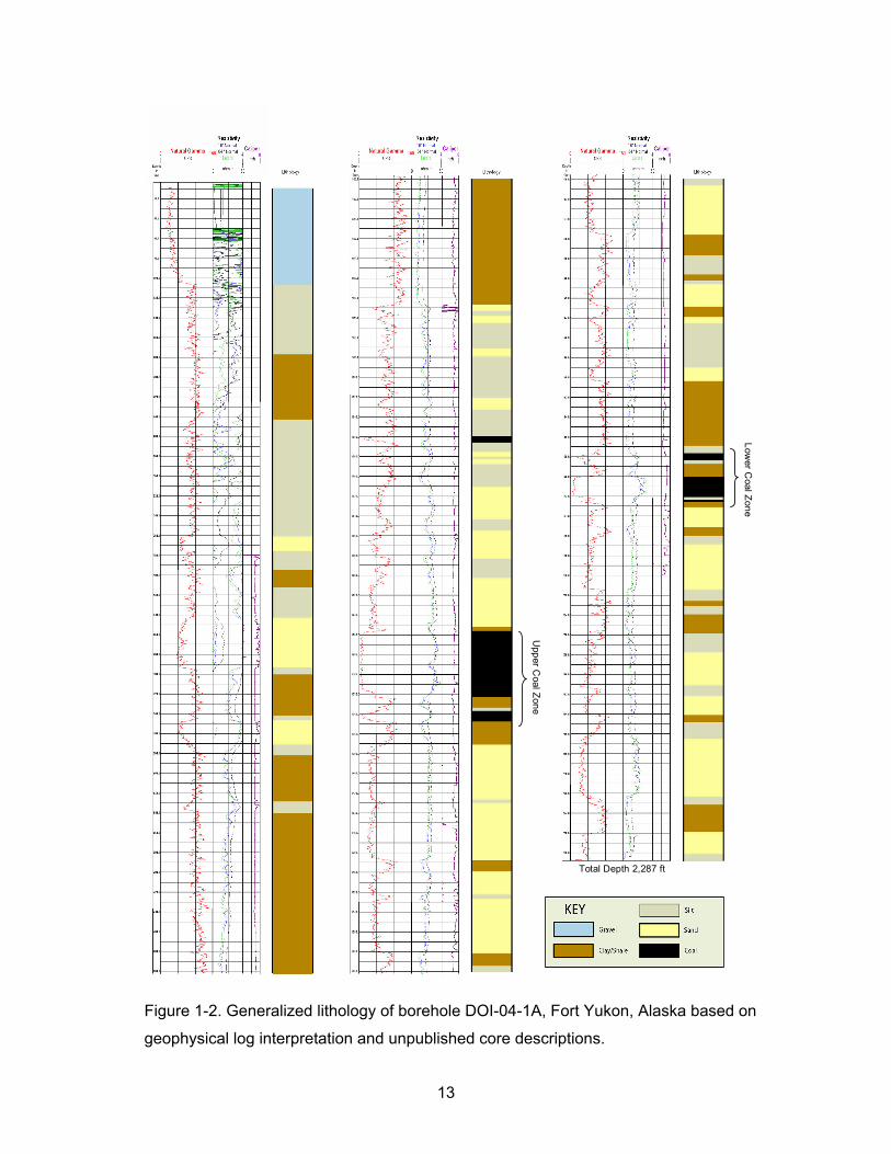
A generalized lithologic log of the penetrated strata, based on geophysical log

interpretation and unpublished core descriptions by the USGS (Ager, T.A., and Fouch, T.D.,

1995, unpub. data) and Alaska DGGS (White, J.G., and Clough, J.G., 2005, unpub. data) is

shown in figure 1-2.

12

Upp

er Coal Z

one

Low

er Coal Z

one

Total Depth 2,287 ft

Figure 1-2. Generalized lithology of borehole DOI-04-1A, Fort Yukon, Alaska based on

geophysical log interpretation and unpublished core descriptions.

13

Geophysical Logging

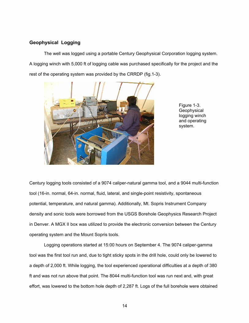
The well was logged using a portable Century Geophysical Corporation logging system.

A logging winch with 5,000 ft of logging cable was purchased specifically for the project and the

rest of the operating system was provided by the CRRDP (fig.1-3).

Figure 1-3. Geophysical logging winch and operating system.

Century logging tools consisted of a 9074 caliper-natural gamma tool, and a 9044 multi-function

tool (16-in. normal, 64-in. normal, fluid, lateral, and single-point resistivity, spontaneous

potential, temperature, and natural gamma). Additionally, Mt. Sopris Instrument Company

density and sonic tools were borrowed from the USGS Borehole Geophysics Research Project

in Denver. A MGX II box was utilized to provide the electronic conversion between the Century

operating system and the Mount Sopris tools.

Logging operations started at 15:00 hours on September 4. The 9074 caliper-gamma

tool was the first tool run and, due to tight sticky spots in the drill hole, could only be lowered to

a depth of 2,000 ft. While logging, the tool experienced operational difficulties at a depth of 380

ft and was not run above that point. The 8044 multi-function tool was run next and, with great

effort, was lowered to the bottom hole depth of 2,287 ft. Logs of the full borehole were obtained

14

using this tool (fig.1-4). However, numerous problems were encountered when attempting to

operate the Mt. Sopris tools with the Century system. Both the tool calibrations and the recorded

borehole footages were off by a considerable amount and, even with repeated attempts to

rectify the problem, could not be reconciled. Both tools were run from a depth of approximately

2,200 ft but, due to the various calibration and compatibility problems, the data gathered were of

marginal quality. Logging operations were completed at 03:00 hours on September 5.

15

Figure 1-4. Geophysical logs of drill hole DOI-04-1A, Fort Yukon, Alaska

16

Monitor Well Installation

After reviewing core, desorption, and geophysical data, a decision was made to set a

monitor well and collect hydraulic information from the upper coal bed. To seal the well below

1,315 ft, drill rods were lowered to a depth of 2,275 ft and abandonment grout was mixed and

pumped from the bottom up to a depth of 1,330 ft. Bentonite pellets and chip were then poured

through the rods, using tremie-suction methods, to a top depth of 1,313 ft. Several 5-gallon

buckets of cleaned and sorted river gravel were poured on top of the bentonite to a top depth of

1,307 ft. A 2 ½-in., schedule 80, threaded flush-joint, polyvinyl chloride (PVC) monitor well with a

5-ft section of stainless steel pipe attached to the bottom was installed in the well with the open

bottom of the pipe set at a depth of 1,272 ft and a set of rubber formation packers set at 1,265

ft. At ground surface, a coupler was attached to the top of the PVC pipe using glue and screws

and a carbide-impregnated sandwich clamp was secured to the PVC pipe immediately below

the coupler. The clamp was then set on the 8 5/8-in. steel surface casing so that the full weight of

the PVC pipe was suspended from the clamp. A 1 ½-in. stainless steel tremie pipe was inserted

into the annular area between the borehole wall and the PVC pipe and ten 5-gallon buckets of

¼-in. bentonite pellets poured through the pipe and placed on top of the rubber packers.

Abandonment grout was then mixed and pumped through the pipe from the top of the bentonite

pellets to within 20 ft of ground surface. Portland cement was mixed and poured in the top 20 ft.

This left the well with 42 ft of isolated open-hole monitor zone in the coal from 1,265 to 1,307 ft.,

with gravel extending to a depth of 1,313 ft (fig. 1-5A). The 1 ½ -in. tremie pipe was removed

from the annular area, cleaned, and lowered into the monitor well to a depth of 1,300 ft. Fresh

water was then slowly circulated through the well to remove drill mud and other material from

the coal and the well.

17

Well Development and Testing

After circulating the drill mud from the monitor well, a portable air compressor (350 psi,

185 cfm) borrowed from the Air Force facility was used to develop the well using air lift methods.

The tremie pipe was pulled to within 200 ft of land surface and compressed air was circulated

through the pipe from progressively greater depths. On September 7, well development was

conducted from depths of 200, 300, 400, and 500 ft with minimum water being produced from

the well. After monitoring water-level recovery at 500 ft with a hand-held water-level meter,

development was continued at a depth of 600 ft. However, as fluid inside the casing was

removed from progressively greater depths, the pressure differential between the outside and

the inside of the casing increased correspondingly. As a result, during air development at 600 ft,

the downward pressure exerted on the rubber formation packers exceeded the holding capacity

of the coupler secured to the top of the PVC pipe. As a result, the coupler sheared and the

casing slipped through the carbide sandwich clamp, falling approximately 35 ft into the well

before coming to rest on the gravel at 1,307 ft (fig. 1-5B). Due to the cold ground temperatures,

the Portland cement that had been pumped into the upper 20 ft of the annular area had not

properly cured and thus did not prevent the pipe from falling down the hole. Rather than latching

onto the casing and attempting to pull it back to land surface, which would likely have resulted in

the fracture of the casing and the total loss of the well, two 20-ft sections of 2 ½-in. PVC pipe,

with a coupler attached face down, were lowered down the well and slipped over the top of the

existing casing at 35 ft. This effectively extended the top of the well back to ground surface but

theoretically decreased the monitored area in the well to the open zone between 1,300 and

1,307 ft and the gravel-filled zone between 1,307 and 1,313 ft (fig. 1-5C). The air development

pipe was then pulled back to 300 ft and, using the air compressor, the well was cleared of fluid

in 100 ft intervals to a depth of 800 ft. With only a minimal amount of water being produced,

development was discontinued and a 1,000 psi pressure transducer placed in the well to a

depth of 780 ft to collect overnight water recovery data.

18

lignite: 1,257-1,315 ft

Lignite

Cement

Bentonite grout

Gravel pack

Bentonite pellets

Open hole - air

A B C

Open hole - water

KEY

Figure 1-5. A. Initial configuration of monitor well DOI-04-1A; B. Configuration of monitor well after casing had slipped; C. Configuration of monitor well after casing was extended back to land surface.

On the morning of September 8, after reviewing the water recovery data, air

development resumed at depths of 800, 900, and 1,000 ft with small water samples being

collected for water-quality analysis. After installing the pressure transducer to 1,020 ft and

collecting water-recovery data for two hours, a decision was made to again flush the well with

fresh water in an attempt to clean the gravel and improve water production. The development

pipe was ultimately lowered to a depth of 1,280 ft and fresh water circulated through the well

before pulling the pipe back and continuing air development from 200 and 300 ft. With the well

still producing minimal water, the development pipe was removed from the well and the

transducer installed to a depth of 400 ft to collect overnight recovery data.

19

On September 9, after reviewing the overnight data, it was apparent that the amount of

water being produced from the well was so small that further efforts at well development were

futile. A pressure transducer was placed in the well to a depth of 600 ft to collect over-winter

pressure data. Additionally, two lengths of heat trace were placed in the well to depths of 275 ft

and 350 ft so that the permafrost portion of the well (approximately 300 ft) could be thawed and

the transducer recovered in the spring of 2005. A 5-ft section of vented 14-in. diameter pipe was

placed and cemented over the well to serve as a protective cover during the winter months

(fig.1-6). The equipment was then cleaned, winterized, packed, and parked at the Air Force

facility.

Figure 1-6. Fort Yukon drill site at conclusion of 2004 drilling operations with protective cover placed over well.

Spring 2005 Activities

A two-man crew flew to Fort Yukon on May 7, 2005 to thaw the well, remove the

transducer, decommission the well, and prepare the equipment to be barged back to Nenana.

After installing batteries and getting the equipment running, the heat traces were plugged in

20

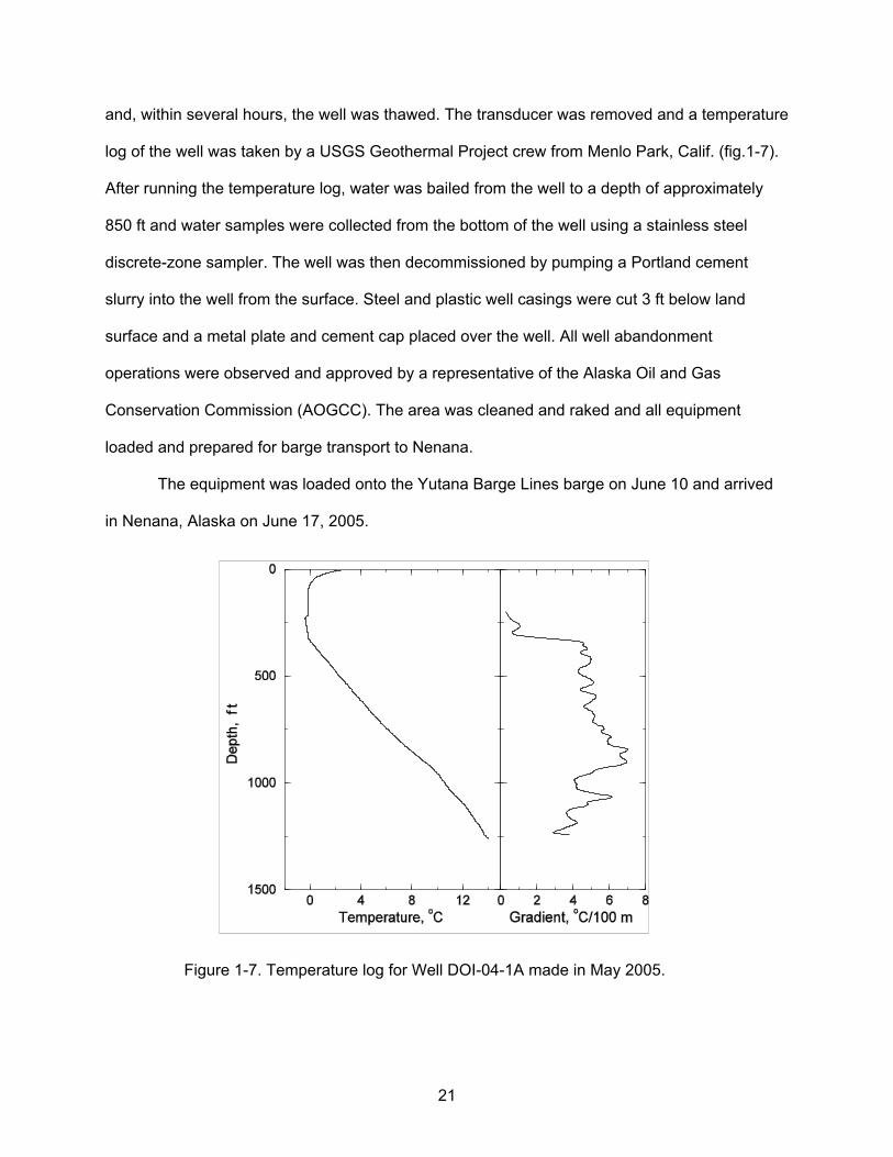
and, within several hours, the well was thawed. The transducer was removed and a temperature

log of the well was taken by a USGS Geothermal Project crew from Menlo Park, Calif. (fig.1-7).

After running the temperature log, water was bailed from the well to a depth of approximately

850 ft and water samples were collected from the bottom of the well using a stainless steel

discrete-zone sampler. The well was then decommissioned by pumping a Portland cement

slurry into the well from the surface. Steel and plastic well casings were cut 3 ft below land

surface and a metal plate and cement cap placed over the well. All well abandonment

operations were observed and approved by a representative of the Alaska Oil and Gas

Conservation Commission (AOGCC). The area was cleaned and raked and all equipment

loaded and prepared for barge transport to Nenana.

The equipment was loaded onto the Yutana Barge Lines barge on June 10 and arrived

in Nenana, Alaska on June 17, 2005.

Figure 1-7. Temperature log for Well DOI-04-1A made in May 2005.

21

Results

The drilling of the 2004 Fort Yukon CBM test well confirmed that portable drilling

equipment can effectively be used to conduct initial CBM assessment drilling in remote areas

where little-to-no subsurface information exists. Although numerous difficulties were

encountered during the project, the data required to make a preliminary determination

concerning the viability of local-use CBM production were collected in a timely and economic

fashion. However, as with any such project, there were lessons learned that can be applied to

similar future operations.

Given more time, it would have been preferable to collect continuous core through the

entire well bore rather than selectively coring in coal-bearing zones only. This is especially

important in areas such as Fort Yukon where virtually no subsurface data exists. Even with the

collection of drill cuttings, it is often difficult to quickly identify borehole lithology when

conducting rotary drilling operations. This allows for the possibility of drilling through relatively

thin coal beds or other strata before identifying them as zones of interest. Even though the coal

bed encountered at 1,900 ft during rotary drilling in DOI-04-1A was quickly identified so that

adequate core samples could be obtained, the upper ten ft of the bed were not cored and

therefore not available for desorption or analyses. In areas that contain relatively thin coal beds,

rather than the substantial coal beds encountered at Fort Yukon, this could prove problematic.

Although the selective core approach may continue to be necessary for future projects due to

time or budgetary constraints, the increased data gathered during continuous coring operations

is probably worth the increased effort and cost.

Due to the portable nature of the equipment used during the drilling operations, the

drill/core rods purchased and used for this project were thin-walled and light-weight in nature.

This does not pose a problem for continuous core drilling operations and allows for a maximum

well-bore depth to be obtained. However, when using these rods for open-hole rotary drilling,

the increased torque and stress transferred to the rods significantly increases the possibility of

22

rod and (or) rod thread fatigue and failure. Although no rods were fractured during the 2004

project, several hundred feet of rods suffered non-repairable thread damage due to excessive

torque and “snap” exerted on them during rotary drilling and could no longer safely be used.

Although the time and money involved in rotary drilling is significantly less than core drilling, if

fracture of the light-weight core rods does occur, the possibility exists of losing the entire

borehole. If this does happen, it will become necessary to utilize the core rods for coring

purposes only.

Due to time and budget constraints, a decision was made to drill the Fort Yukon

borehole, desorb the coal cores, and obtain geophysical logs, before choosing one coal bed

from which to collect hydraulic data. Based primarily on its greater thickness, it was decided to

collect hydraulic data from the upper coal bed at 1,256 ft rather than the lower bed at 1,900 ft.

Therefore, no hydraulic data was collected from the lower coal bed even though it ultimately

contained more methane on a standard cubic feet per ton (scf/ton) basis than did the upper bed

(see section 2, p. 31). In hindsight, the collection of hydraulic data is of such importance when

analyzing reservoir properties and production potential that priority efforts should be made to

collect such data from all significant gas-bearing coal beds. This can be accomplished in one of

two ways: (1) upon coring through the base of a significant gas-bearing coal bed, discontinue

the drilling process, isolate the zone using a single inflatable pneumatic packer system, and

collect discreet-zone hydraulic data; or (2) at the completion of all drilling, coring, and

geophysical logging operations, use an inflatable straddle-packer system to isolate individual

coal beds and collect the required data. Although leaving packers inflated in a fluid-filled

borehole during the data collection process increases the risk of sticking the rods and losing the

well, the importance of the data is such that, with proper precautionary measures, the benefits

probably outweigh the risks involved in the collection process.

23

24

All core and cuttings samples collected from borehole DOI-04-1A have been transferred

to the Alaska Geologic Materials Center in Eagle River, Alaska (contact Dr. John Reeder, 907-

696-0079) and released to the public.

Section 2: Canister Desorption Results from the DOI-04-1A Well, Fort Yukon, Alaska

By Charles Barker1, Arthur Clark2, Beth Maclean3, Karen Clautice4, and Amy Rodman5

Introduction

The Fort Yukon coalbed methane (CBM) assessment study was conducted by

reentering a 1994 USGS core hole to sample coal found in Tertiary strata in the Yukon Flats

Basin (Ager, T.A., 2005, unpub. data). The 1994 well encountered a coal bed at 1,256 ft and

cored 26 ft of coal before drilling was stopped at 1,282 ft, still in coal. In 1994, it was noted that

gas was bubbling from the coal core but desorption testing of the coal was not possible at that

time. Consequently, the reentry of the 1994 well, now officially named DOI-04-1A, was designed

to test the methane content of the coal.

DOI-04-1A well (API no. 50-091-20001) is located at lat 66.55949°N. and long

145.20616°W. The total depth of the well was 2,287 ft. The strata encountered consisted of

about 100 ft of gravel, followed primarily by sandstone, shale, siltstone, and coal associated with

Pliocene to Miocene lake beds deposited some 1.5 to 15 million years ago (Ager, T.A., 2005,

unpub. data). Permafrost was encountered in the well from just below the surface to a depth of

about 300 ft. The well penetrated two primary coal zones: the shallower coal zone extended

from 1,256 to1,345 ft and contained one major coal bed from 1,256 to 1,315 ft and a second

________________________________________________________________________________________________________________________

1 Corresponding author, Scientist Emeritus, U.S. Geological Survey, Denver, Colo., phone: (303) 236-5797 email: barker@usgs.gov

2 U.S. Geological Survey, Denver, Colo. 3 Alaska Division of Geological and Geophysical Surveys, Fairbanks, Alaska 4 Bureau of Land Management, Anchorage, Alaska 5 University of Alaska, Fairbanks

25

coal bed from 1,340 to 1,345 ft. The deeper coal zone extended from 1,878 to 1,926 ft with a

major coal bed from 1,900 to 1,920 ft. The net coal thickness for the primary coal beds in the

two coal zones was 84 ft. Thin or high-ash coals, as picked from geophysical logs (fig. 2-1) at

1,061 to 1,063 ft, 1,878 to 1,882 ft, and queried coal at 2,024 ft, 2,030 ft, 2,038 ft, and 2,056 ft

were not sampled for desorption.

26

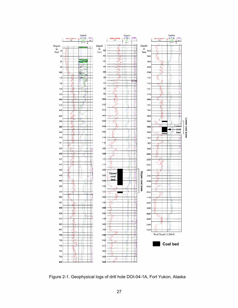
Figure 2-1. Geophysical logs of drill hole DOI-04-1A, Fort Yukon, Alaska

27

DesorptionTechnique

Coal desorption followed a modified U.S. Bureau of Mines (USBM) canister desorption

method as described by Diamond and Levine (1981), Close and Erwin (1989), Ryan and

Dawson (1993), McLennan and others (1994), Mavor and Nelson (1997), and Diamond and

Schatzel (1998) as adapted and modified by Barker and others (1991, 2002) for the use of PVC

canisters. Another major modification of the USBM technique in this study was the use of zero-

headspace canisters (Barker and Dallegge, 2005) in which the headspace is filled with distilled

water rather than with helium gas as described in Barker and others (2002). For this study, the

distilled water was chilled to the approximate drilling mud temperature of 45 to 50 °F prior to

adding it to the canister to minimize the time required to equilibrate the can and coal core to the

lost-gas temperature. Because it is not necessary to measure internal can temperature for a

headspace correction when using zero headspace canisters (Barker and Dallegge, 2005), a

desorption log form modified from Barker and others (2002) was used to allow for this

difference. All canisters were pressure tested for leaks at 6 PSI over a period of at least 24

hours prior to use.

Lost-Gas Estimate

Lost gas is the unmeasured gas desorbed from coal core from the time it is lifted from

the bottom of the well until it is sealed within the canister. Lost gas is controlled by the coal

diffusivity, cleat spacing, and the length of time required to retrieve a given sample and is

estimated by measuring the apparent early rate (first two to four hours) of gas desorption from

the sample sealed within the canister. Lost gas is estimated by plotting cumulative desorbed

gas volume versus the square root of time since the core was lifted off bottom (zero time), and

28

extrapolating the early data, which should form a straight line, back to zero time. The absolute

value of the cumulative volume at the zero-time intercept of this straight line indicates the

volume of lost gas.

In coalbed methane drilling conducted in the Maverick basin in Texas, the Nenana and

Cook Inlet basins in Alaska, and again at DOI-04-1A, the temperature measured at the center of

a freshly opened core face closely tracks the drill mud temperature used to cut the core (unpub.

USGS data), implying that as the core is being cut in the drill hole, it quickly equilibrates to the

drill mud temperature. As a result, once the core retrieval process starts and sample desorption

begins (assumed to be at time zero in the USBM method), the mud temperature to which the

core has equilibrated is the relevant temperature for estimating gas diffusion from the coal

matrix during the lost-gas period rather than the in-situ reservoir temperature. Therefore, during

the period used to determine lost gas, the canisters were desorbed at ambient mud temperature

as discussed in Barker and others (2002). Digital infrared thermometers were used to monitor

drilling mud, core-face, and tank temperature throughout the project. Towards the conclusion of

the project, tank temperatures were allowed to rise to room temperature (65 to 70 °F) in

preparation for canister transport from the drill site to the laboratory in Denver, Colo.

Sampling Desorbed Gas

After the lost gas period had ended, selected core canisters were not measured for

several hours allowing them to accumulate enough gas to collect for analysis. Gas samples

were collected in evacuated 75 ml stainless steel cylinders equipped with needle valves to

control gas flow and seal the cylinder after sampling, by attaching the cylinders directly to the

desorption canister via quick-connect fittings, opening the needle valve for a few seconds, and

then closing the valve and disconnecting the cylinder. This method of gas sampling provided a

sealed sample in a sturdy, transportable container and minimized atmospheric contamination.

29

Analysis of Desorption Data

Correction of the data to standard temperature and pressure (STP) and preparation of a

lost-gas estimate uses a spreadsheet described in Barker and others (2002).

Coring Operations

The 2004 reentry well, DOI-04-1A, was spudded on August 22, 2004 by reentering the

existing 100 ft steel casing set for the 1994 USGS well. After reaming to the bottom of the 1994

borehole (see Section 1, p.11) and collecting reamed cutting samples for desorption from the 27

ft of coal cored at the bottom of the 1994 borehole (1,256 to 1,283 ft; canister sample cuttings 1,

2, 3 in table 2-1A), core drilling began on August 26 at a depth of 1,283 ft.

Because the first 27 ft of the upper coal bed was not cored, and the full thickness of the

bed was not known, all coal recovered from the first two core runs were placed in canisters for

desorption to ensure that adequate data from this bed were collected. After eight canisters had

been filled, a decision was made to only desorb every other foot of coal. Although core recovery

in the coal zone was very good (91 percent), some coal core was lost during the coring and core

retrieval process. In some cases the lost coal cores were recovered on the next core run and

placed in canisters since they should have retained their gas by staying at the hydrostatic

pressure extant at the bottom of the well. Continuous core was drilled to a depth 1,835 ft with

coal encountered from 1,283 to 1,315 ft and 1,340 to 1,345 ft. Thus, the upper major Fort Yukon

coal zone lies at depths from 1,256 to 1,345 ft (fig. 2-1) and contains 64 ft of net coal. In an

attempt to maximize the final depth of the well, and because no coal had been encountered for

almost 500 ft, a decision was made to discontinue coring activities at 1,835 ft and to resume

open-hole drilling until another significant coal bed was reached.

A second significant coal bed was encountered at 1,900 ft and was penetrated for 5 ft

before drilling was stopped. All drill cuttings were circulated from the well and another 5 ft drilled

30

to confirm the presence of a significant coal bed. The resulting cuttings from 1,905 to 1,910 ft

confirmed the presence of a significant coal bed and were collected and placed into canisters

104-31 and 104-32 for desorption. Coring commenced at 1,910 ft and continued to 1,965 ft with

a total of 10 ft of additional coal core being taken from 1,910 to 1,920 ft. This core was placed in

canisters 104-33 to 104-42 (table 2-1B) for desorption. With the subsequent gamma log

indicating the presence of a thin high-ash coal or carbonaceous shale at a depth of 1,878 to

1,882 ft, and a thin carbonaceous shale at 1,925 ft, the lower coal zone extends from

approximately 1,878 to 1,926 ft (fig. 2-1) and contains 20 ft of net coal and 5 ft of high-ash coal

or carbonaceous shale.

Rotary drilling was resumed at 1,965 ft and the borehole reached a final depth of 2,287 ft

on September 3 with no further coal beds encountered or core samples collected.

Results

Desorption

The raw gas content of the upper coal bed core samples average 13.1 standard cubic

feet (scf)/ton with a standard deviation of 3.5 scf/ton for 21 samples (table 2-1A). The raw gas

content of the lower coal bed core samples average 19.1 scf/ton with a standard deviation of 4.0

scf/ton for 10 samples (table 2-1B).

Coal Quality

The upper coal bed, as determined from 21 coal core samples, has a moisture content

averaging 41.25 wt.-percent, consistent with its lignite rank (table 2-2A). This coal bed also

averages 4.10 wt.-percent ash and has an average specific gravity of 1.34, a typical value for

low-ash coal.

31

The lower coal bed, as determined from 10 coal core samples, has a lower moisture

content averaging 31.98 wt.-percent, an ash yield averaging 15.73 wt.-percent and a specific

gravity of 1.48 (table 2-2B).

Desorbed Gas Analyses

Four gas samples taken from canisters 104-1, 104-18, 104-37 and 104-40 were sent to

Isotech Laboratories, Champaign, Ill. for their NG-1 level compositional and isotopic analyses

plus CO2 carbon isotope analyses. All of the gas samples have a significant content of O2, N2,

and CO2 that might represent either release of these gases from in situ sorption sites, from

atmospheric contamination of the coal cores while exposed to air during sampling, or a

combination of the two sources. However, the proportion of in-situ O2, N2 and CO2 versus these

gases absorbed from exposure to air during sampling is difficult to separate. Consequently, the

CH4 and CO2 contents, which are key gases in determining the quality of the gas for sales, were

arbitrarily corrected to an O2- and N2-free basis to provide a qualitative assessment of gas

quality. This method presumes that all O2 and N2 are contaminants and that all CH4 and CO2

are natural coalbed gas components.

After correction to an O2- and N2-free basis, the CH4 content of the four gas samples

ranges from 90 to 96 mol-percent and averages 94 mol-percent. The CO2 content ranges from

3.7 to 9.5 mol-percent and averages 5.4 mol-percent. The CH4-rich character of the gas is

reflected in the calculated calorific content of the gas that ranges from 910 to 970 BTU/Mscf and

averages 950 BTU/Mscf on an O2- and N2-free basis. Pure methane has a calorific content of

1,015 BTU/Mscf.

The δ13CCH4 of the four samples ranges from -72 to -76 o/oo and averages -73 o/oo . The

δ2HCH4 for these samples ranges from -318 to -331 o/oo and averages -324 o/oo. Methane with

this isotopic signature suggests a biogenic source for the gas (Whiticar, 1999), with no apparent

thermogenic component.

32

Coalbed Saturation from Isotherms

Methane adsorption isotherms are measured by reintroducing methane to a coal sample

and measuring the equilibrium gas content at a given pressure and at a constant temperature,

generally the reservoir temperature. Sorption isotherms were developed for one sample each

from the upper and lower coal beds, both at a temperature of 15 ºC, since a temperature log for

the well after it had thermally re-equilibrated with the formation was not available at the time

isotherm analyses were conducted. The resulting curves (figs. 2-2, 2-3) can be used with the

measured gas content from canister desorption (tables 2-1A, 2-1B) to estimate degree of

saturation and the reduction in reservoir pressure needed to saturate the coal with methane,

important factors when evaluating coal bed production potential. The sorption isotherm for the

upper coal bed should be reliable as the May 2005 temperature log indicates a formation

temperature at a depth of 1,260 ft of about 14 ºC (fig. 2-4), nearly the same as the isotherm

temperature. The degree of saturation for the upper coal bed, as calculated in figure 2-2, is 31

percent and the reduction in reservoir pressure required to saturate the coal bed with methane

is 435 psi. The sorption isotherm for the lower coal bed (fig. 2-3) may overstate its in-situ

sorption capacity, as the May 2005 temperature log indicates a geothermal gradient for the

interval between the bottom of the permafrost zone and the depth of 1,260 ft of about 5 ºC/100

m or 2.7 ºF/100 ft. Assuming that gradient persists to the depth of the lower coal bed, its

temperature would be about 24 ºC. Sorption capacity decreases with increasing temperature,

and the degree of saturation for the lower coal bed of 37 percent, as calculated in figure 2-3,

may be somewhat low. The curve also indicates that the reduction in reservoir pressure

required to saturate the coal bed with methane is about 580 psi, a value that may be somewhat

high, due to the temperature effect on the isotherm. Regardless, these values indicate that the

coal beds are undersaturated and imply that reservoir pressure would have to be reduced by

several hundred PSI before methane would be desorbed from the coals.

33

Canister 104-5 , upper coal bed1,287–1,288 ft depth

Gas content on as-received basis = 11.6 scf/ton

Indicated methane storage capacity = 37 scf/ton

Percent saturation = (11.6 / 37) X 100% = 31%

Figure 2-2. Methane adsorption isotherm for canister 104-5 at 1,287–1,288 ft depth in the upper

coal bed, DOI-04-1A well, Fort Yukon, Alaska. Isotherm conditions were: 15 oC, coal at

equilibrium moisture. Absorbed methane values reported on an as-received basis. Coal bed

pressures calculated using a fresh water hydrostatic gradient of .433 psi per ft projected to the

sample depth.

34

Canister 104-33, lower coal bed1,919–1,920 ft depth

Gas content on as-received basis = 20.9 scf/ton

Indicated methane storage capacity = 57 scf/ton

Percent saturation = (20.9 / 57) X 100% = 37%

Figure 2-3. Methane adsorption isotherm for canister 104-33 at 1,910–1,911 ft depth in the

lower coal bed, DOI-04-1A well, Fort Yukon, Alaska. Isotherm conditions were: 15 oC, coal at

equilibrium moisture. Absorbed methane values reported on an as-received basis. Coal bed

pressures calculated using a fresh water hydrostatic gradient of .433 psi per ft projected to the

sample depth.

35

Figure 2-4. Temperature log for well DOI-04-1A made in May 2005.

REFERENCES

Barker, C.E., Johnson, R.C., Crysdale, B.L., and Clark, A.C.,1991, A field and laboratory

procedure for desorbing coal gases: U.S. Geological Survey Open-File Report OF 91–

0563, 14 p.

Barker, C.E., Dallegge, T.A., and Clark, A.C., 2002, USGS coal desorption equipment and a

spreadsheet for analysis of lost and total gas from canister desorption measurements:

U.S. Geological Survey Open-File Report OF 2002–496, 13 p. plus spreadsheet.

36

Barker, C.E., and Dallegge, T.A., 2005, Zero-headspace coal-core gas desorption canister,

revised desorption data analysis spreadsheets and a dry canister heating system: U.S.

Geological Survey Open-File Report OF 2005–1177, 9 p.

Close, J.C., and Erwin, T.M., 1989, Significance and determination of gas content data as

related to coalbed methane reservoir evaluation and production implications: Proceedings

of the 1989 Coalbed Methane Symposium, paper 8922, p. 37–55.

Diamond, W.P., and Levine, J.R., 1981, Direct method determination of the gas content of coal:

procedures and results: U.S. Bureau of Mines Report of Investigations 8515, 36 p.

Diamond, W.P., and Schatzel, S.J., 1998, Measuring the gas content of coal: a review, in

Flores, R.M., ed., Coalbed methane: from coal-mine outbursts to a gas resource:

International Journal of Coal Geology, v. 35, p. 311–331.

Mavor, M., and Nelson, C.R., 1997, Coalbed reservoir gas-in-place analysis: Gas Research

Institute Report no. GRI-97/0263, 134 p.

McLennan, J.D., Schafer P.S., and Pratt, T.J., 1994, A guide to determining coalbed gas

content: Gas Research Institute, variously paginated.

Ryan, B.D., and Dawson, F.M., 1993, Coalbed methane canister desorption techniques; in

Grant, B. and Newell, J.M. eds., Geological fieldwork 1993: B.C. Ministry of Energy,

Mines, and Petroleum Resources, Paper 1994-1, p. 245–256.

37

Whiticar, M.J. 1999, Carbon and hydrogen isotope systematics of bacterial formation and

oxidation of methane: Chemical Geology v. 161, p. 291–314.

38

Table 2-1A. Summary of canister desorption results, upper coal zone.

Canister number

Depth interval

Canister sample lithology

Raw coal mass

Lost gas

estimate

Total raw gas content

Upper coal zone

Top

Bottom

(as-received basis)

(feet) (feet) % coal (g) (cc) (scf/ton)

CORE

104-1 1,283 1,284 100 1,056 60 14.1 104-2 1,284 1,284.5 50 490 40 13.5 104-3 1,285 1,286 100 907 85 10.8 104-4 1,286 1,287 100 905 80 9.8 104-5 1,287 1,288 100 951 80 11.6 104-6 1,288 1,289 100 1,009 115 21.1 104-7 1,289 1,290 100 1,149 85 7.0 104-8 1,290 1,290.7 70 471 85 14.5 104-9 1,295 1,296 100 961 85 13.4

104-10 1,304.5 1,305.5 100 1,087 110 13.8 104-11 1,306.5 1,307.5 100 1,193 95 12.1 104-12 1,308.5 1,309.5 100 1,115 130 13.6 104-13 1,310.5 1,311.5 100 1,132 130 13.9 104-14 1,312.5 1,313.5 100 842 80 11.0 104-15 1,315 1,316 100 1,038 80 12.9 104-16 1,319 1,320 100 1,171 85 8.6 104-17 1,324 1,325 100 1,518 100 9.0 104-18 1,339.7 1,340.7 100 1,082 100 18.7 104-19 1,342

1,343

100 749 100 19.5

104-20 1,343

1,344

100 1,028 110 15.2

104-21 1,344

1,345

100 1,098 100 10.9

Statistics: Sample mean 13.1

Standard deviation 3.5 CUTTINGS Cuttings-1* 1,265 1,270 80 575 45 7.7 Cuttings-2* 1,270 1,275 80 609 20 4.6 Cuttings-3* 1,275

1,280 80 886 20 2.0

Statistics: Sample mean 4.8 Standard deviation 2.9

* Depth interval estimated from lag time. These cuttings were not screened and the coal fines lose their gas quickly, thought to lead to the spuriously low raw gas content.

Abbreviations: g, grams; cc, cubic centimeters; scf, standard cubic feet

39

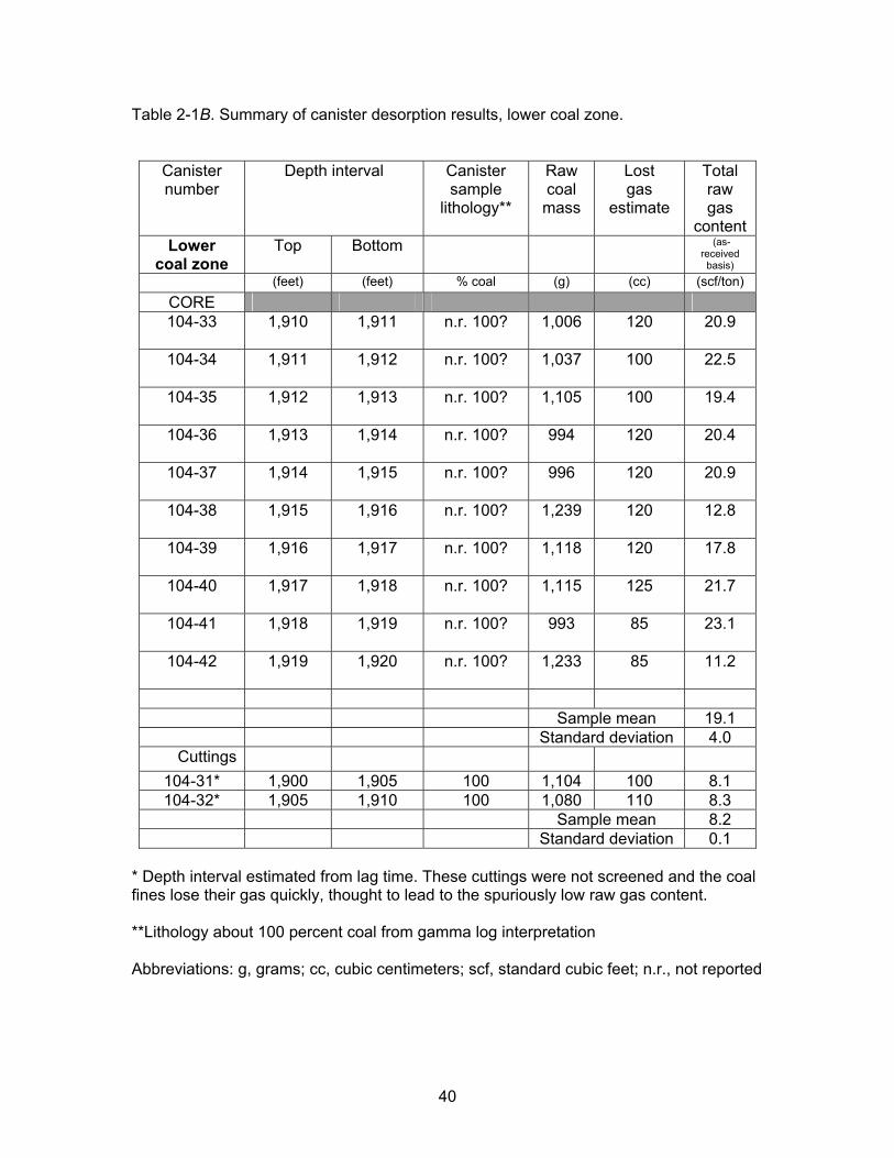
Table 2-1B. Summary of canister desorption results, lower coal zone.

Canister number

Depth interval

Canister sample

lithology**

Raw coal mass

Lost gas

estimate

Total raw gas

content Lower

coal zone Top

Bottom

(as-

received basis)

(feet) (feet) % coal (g) (cc) (scf/ton)

CORE 104-33 1,910 1,911

n.r. 100? 1,006 120 20.9

104-34 1,911

1,912

n.r. 100? 1,037 100 22.5

104-35 1,912

1,913

n.r. 100? 1,105 100 19.4

104-36 1,913

1,914

n.r. 100? 994 120 20.4

104-37 1,914

1,915

n.r. 100? 996 120 20.9

104-38 1,915

1,916

n.r. 100? 1,239 120 12.8

104-39 1,916

1,917

n.r. 100? 1,118 120 17.8

104-40 1,917

1,918

n.r. 100? 1,115 125 21.7

104-41 1,918

1,919

n.r. 100? 993 85 23.1

104-42 1,919

1,920

n.r. 100? 1,233 85 11.2

Sample mean 19.1 Standard deviation 4.0

Cuttings

104-31* 1,900 1,905 100 1,104 100 8.1 104-32* 1,905 1,910 100 1,080 110 8.3

Sample mean 8.2 Standard deviation 0.1

* Depth interval estimated from lag time. These cuttings were not screened and the coal fines lose their gas quickly, thought to lead to the spuriously low raw gas content.

**Lithology about 100 percent coal from gamma log interpretation

Abbreviations: g, grams; cc, cubic centimeters; scf, standard cubic feet; n.r., not reported

40

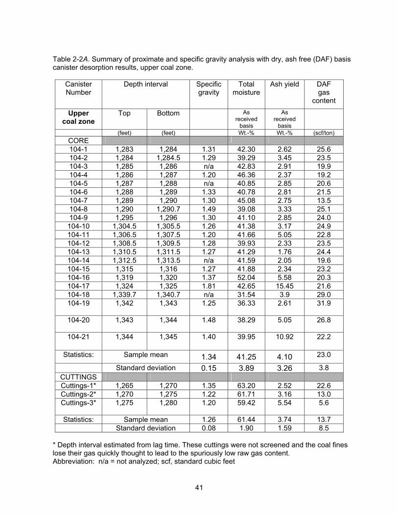
Table 2-2A. Summary of proximate and specific gravity analysis with dry, ash free (DAF) basis canister desorption results, upper coal zone.

Canister Number

Depth interval

Specific gravity

Total moisture

Ash yield DAF gas

content

Upper coal zone

Top

Bottom

As received

basis

As received

basis

(feet) (feet) Wt.-% Wt.-% (scf/ton)

CORE

104-1 1,283 1,284 1.31 42.30 2.62 25.6 104-2 1,284 1,284.5 1.29 39.29 3.45 23.5 104-3 1,285 1,286 n/a 42.83 2.91 19.9 104-4 1,286 1,287 1.20 46.36 2.37 19.2 104-5 1,287 1,288 n/a 40.85 2.85 20.6 104-6 1,288 1,289 1.33 40.78 2.81 21.5 104-7 1,289 1,290 1.30 45.08 2.75 13.5 104-8 1,290 1,290.7 1.49 39.08 3.33 25.1 104-9 1,295 1,296 1.30 41.10 2.85 24.0

104-10 1,304.5 1,305.5 1.26 41.38 3.17 24.9 104-11 1,306.5 1,307.5 1.20 41.66 5.05 22.8 104-12 1,308.5 1,309.5 1.28 39.93 2.33 23.5 104-13 1,310.5 1,311.5 1.27 41.29 1.76 24.4 104-14 1,312.5 1,313.5 n/a 41.59 2.05 19.6 104-15 1,315 1,316 1.27 41.88 2.34 23.2 104-16 1,319 1,320 1.37 52.04 5.58 20.3 104-17 1,324 1,325 1.81 42.65 15.45 21.6 104-18 1,339.7 1,340.7 n/a 31.54 3.9 29.0 104-19 1,342

1,343

1.25 36.33 2.61 31.9

104-20 1,343

1,344

1.48 38.29 5.05 26.8

104-21 1,344

1,345

1.40 39.95 10.92 22.2

Statistics: Sample mean 1.34 41.25 4.10 23.0

Standard deviation 0.15 3.89 3.26 3.8 CUTTINGS Cuttings-1* 1,265 1,270 1.35 63.20 2.52 22.6 Cuttings-2* 1,270 1,275 1.22 61.71 3.16 13.0 Cuttings-3* 1,275

1,280 1.20 59.42 5.54 5.6

Statistics: Sample mean 1.26 61.44 3.74 13.7 Standard deviation 0.08 1.90 1.59 8.5

* Depth interval estimated from lag time. These cuttings were not screened and the coal fines lose their gas quickly thought to lead to the spuriously low raw gas content. Abbreviation: n/a = not analyzed; scf, standard cubic feet

41

Table 2-2B. Summary of proximate and specific gravity analysis with dry, ash free (DAF) basis canister desorption results, lower coal zone.

Canister number

Depth interval

Specific gravity

Total moisture

Ash yield

DAF gas

content Lower

coal zone Top

Bottom

As

received basis

As received

basis

(feet) (feet) Wt.-% Wt.-% scf/ton

CORE 104-33 1,910

1,911

n/a 35.08 7.74 36.5

104-34 1,911

1,912

1.14 34.11 3.78 36.2

104-35 1,912

1,913

1.23 35.73 3.62 32.1

104-36 1,913

1,914

1.39 34.73 5.50 34.1

104-37 1,914

1,915

1.24 34.66 7.75 36.3

104-38 1,915

1,916

1.85 30.17 30.48 32.5

104-39 1,916

1,917

1.81 28.87 27.55 40.9

104-40 1,917

1,918

1.74 27.88 22.64 43.9

104-41 1,918

1,919

1.41 31.16 7.72 37.8

104-42 1,919

1,920

n/a 27.37 40.57 35.0

Sample mean 1.48 31.98 15.73 36.5 Standard deviation 0.28 3.24 13.37 3.6

CUTTINGS 104-31* 1,900 1,905 1.25 55.69 2.8 12.8 104-32* 1,905 1,910 n/a 51.75 3.0 13.1

Sample mean 53.72 2.9 13.0 Standard deviation 2.79 0.1 0.2

* Depth interval estimated from lag time. These cuttings were not screened and the coal fines lose their gas quickly thought to lead to the spuriously low raw gas content.

Abbreviations: n/a, not analyzed; scf, standard cubic feet

42

Section 3: Aquifer Test and Water-Quality Analyses, DOI-04-1A Well, Fort Yukon, Alaska

By Edwin P. Weeks1, Arthur Clark2, and Cindy A. Rice2

Introduction

Methane production from coal requires that the hydraulic pressure maintaining sorption

of the methane on the coal be reduced by co-producing water by pumping. Prediction of the

hydraulic pressure response to pumping within the coal bed and assessment of the potential for

methane production requires knowledge of the coal bed hydraulic properties, to be determined

using aquifer tests. Based on the drilling schedule, only one coal bed was tested. The thick coal

bed in the upper coal zone at a depth of 1,256 to 1,315 ft is substantially thicker than the

thickest coal bed in the lower coal zone, and was initially estimated to have a slightly higher

methane content (refuted after desorption experiments were completed; see tables 3-1A, 3-1B).

Hence, an attempt was made to finish the borehole as a production well in that coal bed,

followed by performance of a single-well aquifer test. Events described below precluded a true

aquifer test, but several sets of recovery data were collected during the development phase,

four of which were analyzed to provide estimates of the coal hydraulic properties.

Production of coalbed methane (CBM) is also contingent on management of coal bed

water co-produced with the methane, requiring knowledge of the quality as well as the quantity

of coalbed water. Consequently, water samples were collected for chemical analysis from the

upper coal bed during well-testing and upon retrieval of the pressure transducer in May 2005.

These samples are less than ideal, as water samples should be taken only after extensive well

________________________________________________________________________________________________________________________

1 Corresponding author, U.S. Geological Survey, Denver, Colo. phone: (303) 236-4981 epweeks@usgs.gov 2 U.S. Geological Survey, Denver, Colo.

43

development to ensure that no drilling fluids or suspended solids alter the formation water

characteristics. However, waiting was not possible during this test, due to the problems outlined

below. Nonetheless, the resulting chemical analyses, augmented by analyses of a squeeze

sample from a siltstone underlying the coal bed, and of water used in the drilling mud and in

flushing the well, appear to be reasonably representative of coal bed waters determined in other

areas, and presumably, then, reliable indicators of the upper coal bed water chemistry.

44

Table 3-1A. Summary of canister desorption results, upper coal zone.

Canister number

Depth interval

Canister sample lithology

Raw coal mass

Lost gas

estimate

Total raw gas content

Upper coal zone

Top

Bottom

(as-received basis)

(feet) (feet) % coal (g) (cc) (scf/ton)

CORE

104-1 1,283 1,284 100 1,056 60 14.1 104-2 1,284 1,284.5 50 490 40 13.5 104-3 1,285 1,286 100 907 85 10.8 104-4 1,286 1,287 100 905 80 9.8 104-5 1,287 1,288 100 951 80 11.6 104-6 1,288 1,289 100 1,009 115 21.1 104-7 1,289 1,290 100 1,149 85 7.0 104-8 1,290 1,290.7 70 471 85 14.5 104-9 1,295 1,296 100 961 85 13.4

104-10 1,304.5 1,305.5 100 1,087 110 13.8 104-11 1,306.5 1,307.5 100 1,193 95 12.1 104-12 1,308.5 1,309.5 100 1,115 130 13.6 104-13 1,310.5 1,311.5 100 1,132 130 13.9 104-14 1,312.5 1,313.5 100 842 80 11.0 104-15 1,315 1,316 100 1,038 80 12.9 104-16 1,319 1,320 100 1,171 85 8.6 104-17 1,324 1,325 100 1,518 100 9.0 104-18 1,339.7 1,340.7 100 1,082 100 18.7 104-19 1,342

1,343

100 749 100 19.5

104-20 1,343

1,344

100 1,028 110 15.2

104-21 1,344

1,345

100 1,098 100 10.9

Statistics: Sample mean 13.1

Standard deviation 3.5 CUTTINGS Cuttings-1* 1,265 1,270 80 575 45 7.7 Cuttings-2* 1,270 1,275 80 609 20 4.6 Cuttings-3* 1,275

1,280 80 886 20 2.0

Statistics: Sample mean 4.8 Standard deviation 2.9

* Depth interval estimated from lag time. These cuttings were not screened and the coal fines lose their gas quickly, thought to lead to the spuriously low raw gas content. Abbreviations: g, grams; cc, cubic centimeters; scf, standard cubic feet

45

 Table 3-1B. Summary of canister desorption results, lower coal zone.

Canister number

Depth interval

Canister sample

lithology**

Raw coal mass

Lost gas

estimate

Total raw gas

content Lower

coal zone Top

Bottom

(as-

received basis)

(feet) (feet) % coal (g) (cc) (scf/ton)

CORE 104-33 1,910 1,911

n.r. 100? 1,006 120 20.9

104-34 1,911

1,912

n.r. 100? 1,037 100 22.5

104-35 1,912

1,913

n.r. 100? 1,105 100 19.4

104-36 1,913

1,914

n.r. 100? 994 120 20.4

104-37 1,914

1,915

n.r. 100? 996 120 20.9

104-38 1,915

1,916

n.r. 100? 1,239 120 12.8

104-39 1,916

1,917

n.r. 100? 1,118 120 17.8

104-40 1,917

1,918

n.r. 100? 1,115 125 21.7

104-41 1,918

1,919

n.r. 100? 993 85 23.1

104-42 1,919

1,920

n.r. 100? 1,233 85 11.2

Sample mean 19.1 Standard deviation 4.0

Cuttings

104-31* 1,900 1,905 100 1,104 100 8.1 104-32* 1,905 1,910 100 1,080 110 8.3

Sample mean 8.2 Standard deviation 0.1

* Depth interval estimated from lag time. These cuttings were not screened and the coal fines lose their gas quickly, thought to lead to the spuriously low raw gas content.

**Lithology about 100 percent coal from gamma log interpretation.

Abbreviations: g, grams; cc, cubic centimeters; scf, standard cubic feet; n.r., not reported

46

Hydrogeologic Setting

The well penetrates about 100 ft of coarse surficial gravel deposited by the Yukon River,

and deeper deposits tapped by the well consist of lacustrine deposits of interbedded clay, silty

clay, silt, silty sand, and sand, with occasional coal beds. Permanent permafrost extends from

about 25 to 300 ft, providing a hydrologic confining layer for the underlying materials. The main

interest of this hydrologic investigation is of the tested upper coal bed and the beds immediately

above and below it, as shown in figure 3-1. The coal bed is immediately overlain by a thin clay

bed, separating it from a sand bed. A thicker clay bed separates the upper coal bed from an

underlying thinner coal that is, in turn, underlain by another thick clay bed. These overlying and

underlying clay beds should provide hydrologic confinement for the upper coal, allowing well

test theory developed for confined aquifers to be applied.

47

A B C

1,200

1,250

1,300

1,350

1,400

De

pth

(ft

)

Sand

Clay

Lignite

Bentonite grout

Gravel

Open hole (water)

casi

ng

casi

ng

Figure 3-1. A. Geologic profile for 1,200–1,400 ft depth interval in DOI-04-1A CBM well, Fort

Yukon, Alaska; B. Original well construction; C. Well configuration after the casing had slipped

downhole by 35 ft. Scale approximate.

Well Completion and Initial Development

Well completion is described in detail in Section 1, but details relevant to interpretation of

the hydraulic tests are briefly summarized here. To complete the well for testing, the borehole

below the base of the upper coal was backfilled with Volclay™ abandonment grout mixed with

thick bentonite, bentonite pellets, and bentonite chips to a depth of 1,313 ft, about 2 ft above the

bottom of the coal bed, providing the bottom depth that would yield water to the well. Gravel was

48

added to a depth of 1,307 ft to prevent bentonite from being pumped up into the planned open-

hole interval. The lead section of well casing (2.5-in. schedule 80 PVC pipe) was equipped with

five 6-in. shale baskets attached 7 ft above the bottom of a stainless steel tail section. The

casing was hung from a clamp at land surface so that the shale baskets (packer) bottomed at

1,265 ft, about 9 ft below the top of the coal. Including the open hole surrounding the tail pipe

and the 6-ft gravel-filled section, the well section open to the coal should have been 48 ft. Ten

buckets of bentonite pellets were placed by tremie pipe immediately above the shale baskets,

and the remainder of the annulus around the well casing was filled with abandonment grout.

Details of well completion through the 1,200–1,400 ft zone are illustrated in figure 3-1.

Following completion of the well, drilling mud remaining in the open portion of the hole

(1,265–1,307 ft) was flushed with fresh water using a tremie pipe installed to a depth of 1,302 ft.

The driller reported that 400 gallons of fresh water were pumped down the casing before mud

began to flow at land surface. The loss of this fluid may have resulted in additional formation

damage and the apparent large skin effect described below.

Well Tests and Slug Test Theory

Following completion of the well, air-lift pumping was initiated to remove fines from the

invaded zone surrounding the well bore in anticipation of the performance of an aquifer test.

Several brief sets of recovery data were collected at various stages of development to provide

data for test planning, but various problems that occurred during development precluded

conducting the aquifer test. However, data for three of the recovery data sets, as well as head

recovery following the end of development were analyzed using slug test theory to obtain

estimates of the hydraulic properties of the upper coal bed.

The slug test theory used was that of Cooper and others (1967), as modified by Butler

(1997, p. 173) to account for the effects of well-bore clogging or the development of a well skin.

The analysis procedure was also modified to that of Earlougher (1977, p. 99) to better analyze

data that represent water level recovery of only a few percent of its initial drawdown.The

analysis relies on matching test data to a selected member of a family of theoretical log-log type

curves of 1-H/H0 vs. KDt/rc2 for various values of , defined as (Butler, 1997, p. 173):

)2exp(* 2

2

sr

Sr

c

w ,

49

where H is the remaining water level displacement, (length); H0 is the initial (instantaneous)

water level displacement, (length); K is aquifer hydraulic conductivity, (length/time); D is screen

or open hole length; t is elapsed time since the instantaneous displacement; rc is casing radius,

(length); rw is the open hole radius, (length); S is the aquifer storage coefficient; and s is

dimensionless skin. Dimensionless skin is defined (Matthews and Russell, 1967, p. 19–21) as: 

w

skin

s r

r

K

Ks ln1  

where Ks is hydraulic conductivity of the clogged annular layer surrounding the borehole,

(length/time); and rskin the outside radius of the clogged layer, (length). In theory, transmissivity,

T, equal to Kb, where b is aquifer thickness, should be the parameter determined by slug test

analysis. However, practice indicates that the T determined from slug tests represents the KD

product, indicating that, at the scale of the slug test, flow to the well bore is governed by the

screen or open-hole length, rather than by the full aquifer thickness (Butler, 1997, p. 52–53).

For analysis, a data plot of 1-H/H0 vs. t, as determined from measurements, is prepared

to the same scale as the type-curve plot. To match the curves, values of 1-H/H0 for the data plot

must coincide with those for the type-curve family, but the logarithmic data time axis is shifted,

by use of a multiplier M, to provide a match of the data to a selected member of the type-curve

family. M is equal to  tr

KDt

c

/2

, where 

2cr

KDt  is the type-curve match line value as read from

the x axis, and t is the time at which the match data point was read. M has the unit of time-1. KD

is then found as . Selection of the type-curve to be matched can be quite subjective,

as the type-curves are of nearly constant shape over a significant range of values.

2cMrKD

Hydraulic conductivity, K, is widely used by hydrogeologists as the hydraulic property

governing the movement of water through porous media. However, because of the need to

consider the flow of various fluids through porous media, petroleum engineers generally use

permeability, k, in units of Darcies, as the parameter-governing porous-media fluid flow. As this

practice has been followed in most of the literature on coal-bed methane development, k values

will also be presented. A permeability of one ft/d is equivalent to 0.43 Darcy at the temperature

of 14 ºC prevailing at the depth of the upper coal bed, as determined from the temperature log

(fig. 1-2) obtained in 2005.

50

Recovery data were either collected by use of an electric tape, by which depth to water

(DTW) was measured directly, or by use of two absolute pressure transducers, one (an In-Situ

Minitroll™ transducer) emplaced at some depth below the water surface in the well and the

other (an In-Situ Barotroll™ transducer) at land surface to record barometric pressure. For the

transducer data, DTW was computed as (DT-[TR-BP]) where DT is depth of emplacement of

transducer below land surface, TR is the transducer pressure reading in ft of water, and BP is

barometric pressure in ft of water as read from the Barotroll transducer. For all tests, the static

water level (SWL) was assumed to be 6 ft below land surface, based on the approximate depth

to water after the well was thawed in May 2005. Starting times for each test were assumed to

coincide with the time at which air-lift pumping was stopped to allow for the test. This represents

an approximation, as slug test theory assumes instantaneous displacement of the initial water

level, whereas air-lift pumping for development was occurring for several hours prior to each

water-level measurement period. However, in each case, the period of air-lift pumping was

small relative to the time required for full water level recovery, and the assumption of

instantaneous displacement was assumed to be adequately met. The initial head displacement

was assumed to be the DTW when pumping was stopped minus the SWL. However, heads

were not monitored during air lift, so the initial DTW was estimated by linearly extrapolating the

average rate of head increase during the test back to the start time. For each of the short

recovery tests, the rate of head recovery was quite uniform with time, so this extrapolation

should create little error.

Test 1

This data set is the first reliable one available and was collected after the casing had

been evacuated of water by air-lift pumping to a depth of 500 ft. Evacuation was accomplished

in stages, beginning with a 200-ft evacuation starting at 08:18 hours on September 7.

Measurements of recovery of the water level for this evacuation were made with an electric

tape, but the readings were later recognized to have been affected by water draining down the

inside wall of the casing, and hence were not reliable. The casing was evacuated in two

additional stages to a depth of 500 ft, and recovery was again measured, after pumping halted

at 11:30 hours. This time, the problem of false readings was noted after a false start, and a

series of six good measurements was obtained, beginning at 11:43:15 hours, and lasting about

51

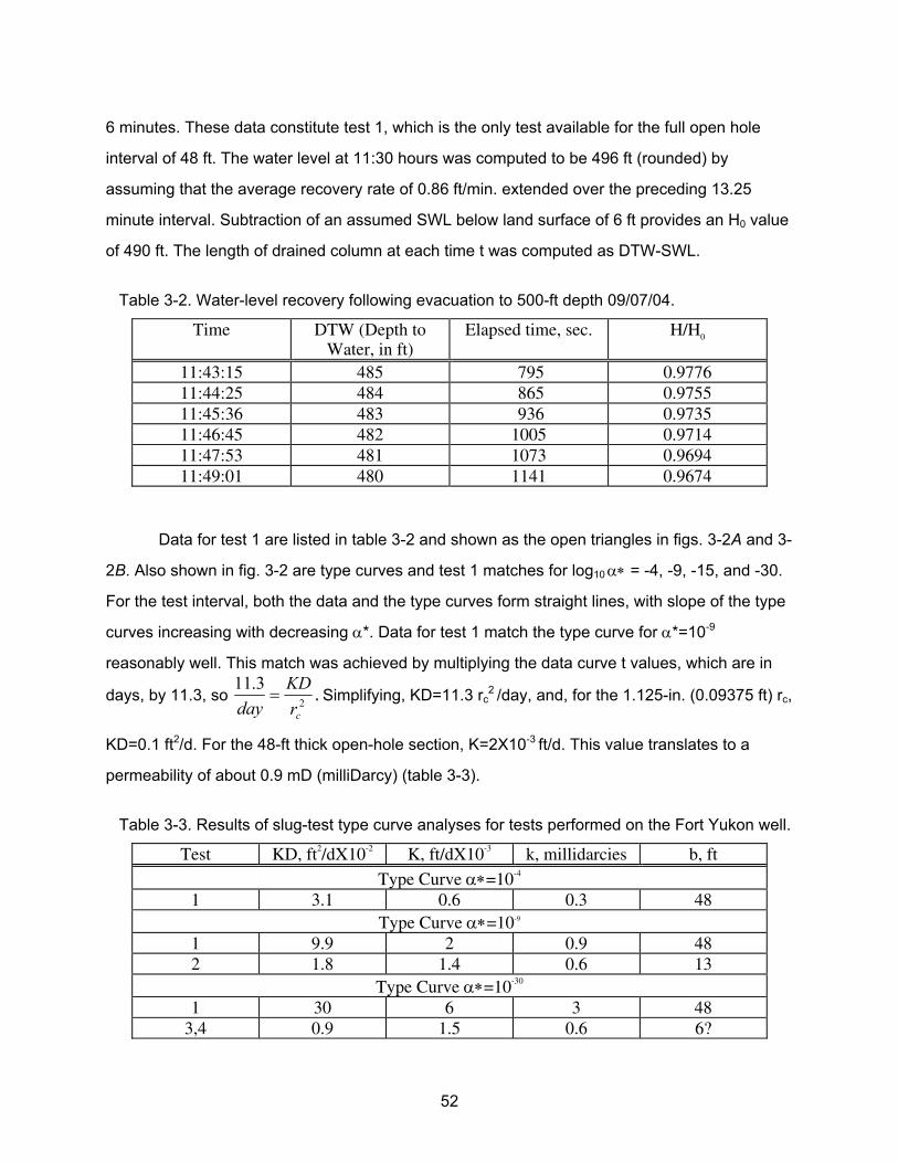
6 minutes. These data constitute test 1, which is the only test available for the full open hole

interval of 48 ft. The water level at 11:30 hours was computed to be 496 ft (rounded) by

assuming that the average recovery rate of 0.86 ft/min. extended over the preceding 13.25

minute interval. Subtraction of an assumed SWL below land surface of 6 ft provides an H0 value

of 490 ft. The length of drained column at each time t was computed as DTW-SWL.

Table 3-2. Water-level recovery following evacuation to 500-ft depth 09/07/04.

Time DTW (Depth to Water, in ft)

Elapsed time, sec. H/H0

11:43:15 485 795 0.9776 11:44:25 484 865 0.9755 11:45:36 483 936 0.9735 11:46:45 482 1005 0.9714 11:47:53 481 1073 0.9694 11:49:01 480 1141 0.9674

Data for test 1 are listed in table 3-2 and shown as the open triangles in figs. 3-2A and 3-

2B. Also shown in fig. 3-2 are type curves and test 1 matches for log10  = -4, -9, -15, and -30.

For the test interval, both the data and the type curves form straight lines, with slope of the type

curves increasing with decreasing *. Data for test 1 match the type curve for *=10-9

reasonably well. This match was achieved by multiplying the data curve t values, which are in

days, by 11.3, so 2

3.11

cr

KD

day . Simplifying, KD=11.3 rc

2 /day, and, for the 1.125-in. (0.09375 ft) rc,

KD=0.1 ft2/d. For the 48-ft thick open-hole section, K=2X10-3 ft/d. This value translates to a

permeability of about 0.9 mD (milliDarcy) (table 3-3). 

Table 3-3. Results of slug-test type curve analyses for tests performed on the Fort Yukon well.

Test KD, ft2/dX10-2 K, ft/dX10-3 k, millidarcies b, ft

Type Curve =10-4 1 3.1 0.6 0.3 48

Type Curve=10-9

1 9.9 2 0.9 48 2 1.8 1.4 0.6 13

Type Curve =10-30 1 30 6 3 48

3,4 0.9 1.5 0.6 6?

52

 

 

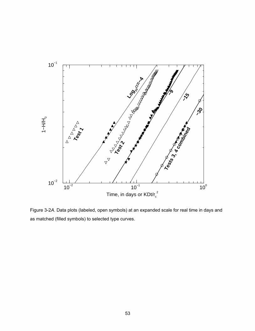
10−2

10−1 100

Time, in days or KDt/rc

2

10−2

10−1

1−H

/H0

Log 10

α=−4

−9

−15

−30

Test

1

Test

2

Test

s 3,

4 c

ombi

ned

 

Figure 3-2A. Data plots (labeled, open symbols) at an expanded scale for real time in days and

as matched (filled symbols) to selected type curves.

53

 

10−2

10−1 100 101 102

Time, in days or KDt/rc

2

10−2

10−1

1001−

H/H

0

Log 10

α=−4

−9 −15

−30

Test

1 Test

2

Test

s 3,

4 c

ombi

ned

 

Figure 3-2B. Same as figure 3-2A, but showing the type curves to include complete recovery.

Type curves generated using Fortran program of Greene and Shapiro (1995).

 The * value of 10-9 was chosen as the maximum value that matched the steepness of

the data curve. The * value that should be matched in the absence of well-bore clogging (s=0),

2

2

c

w

r

Sr , may be determined from well construction data and an estimate of S. Three well-

controlled aquifer tests conducted on sub-bituminous coal beds in the Powder River Basin

provide a specific storage (Ss) for coals of about 6X10-6/ft (Weeks, 2005, p. 254). Although the

48-ft thick (b) coal bed at this site is of lower rank, we assume, due to a lack of other data, a

similar Ss, so we compute S=Ss b=3X10-4. For this well, rw= 3.5 in., and rc=1.125 in. Thus,

=3X10-3, and a match to the *=10-9 type curve indicates substantial clogging. As a plausibility

check, the exp(-2s) value needed to reduce * to 10-9 from 3X10-3 is 3.3X10-7, results in s = 7.5.

54

Assuming a 1-in. thick clogged zone, ln (rskin/rw) is 0.25, so, based on the equation

w

skin

s r

r

K

Ks ln1 , Ks is about 0.03 times that of the formation.

The fact that the log-log plot of head recovery for test 1 is steeper than the type curve

plots for larger *values could be due to ongoing well development as water entering the well

removes fine materials from the well bore wall. In that case, use of the *=10-9 type curve to

analyze the test may over-estimate clogging, and the computed KD value may thus be too

large. To obtain a probable minimum estimate for KD and K, the earliest data were also

matched to the curve, as that may be about the maximum * that would still allow well

development to occur. For this match, KD=3.5rc2, or about 0.03 ft2/d, providing a minimum K

value of 0.6X10-3 ft/d or about 0.3 mD. A maximum estimate of KD and K for this test is more

difficult to estimate. A match of the data to the *=10-30 curve provides a K of 6X10-3 ft/d or 3

mD. A 1-in. clogged layer would have to be about 100 times less permeable than the formation,

within the realm of possibility, but perhaps unlikely at this stage of well completion and

development.

Events Leading to Test 2

Following the end of electric tape recovery measurements at 11:50 hours, tremie pipe

was added and the well was air-lift pumped from a depth of 600 ft until about 13:00 hours, when

the casing slipped through the clamp and fell about 35 ft down the hole, the bentonite grout

presumably slipping with it. Based on the various initial depths of packer, tail section bottom,

and gravel top, the bottom of the well casing was now resting on the gravel surface, with 7 ft of

open hole above the casing bottom. The resulting well configuration is shown in figure 3-1C.

Two new sections of casing were installed over the tremie pipe to salvage the well. Following

the well collapse, a water level depth of about 48 ft was measured in the casing.

Air-lift pumping in the salvaged well was resumed at 15:30 hours, and water levels were

lowered to 500 ft by 16:30 hours. Water level recovery was monitored for several minutes

beginning at 16:45 hours, but recovery was quite slow (about 0.2 ft/min.), with somewhat erratic

behavior, possibly due to water running down the casing. Consequently, no attempt was made

to analyze these data. Pumping resumed about 17:00 hours, and the well was evacuated to a

depth of 780 ft by 18:30. Pumping from that depth continued until 20:10 hours. At that time, 3

55

sections of tremie pipe were added, and the pressure transducer was emplaced at the 780-ft

depth to record recovery overnight, beginning at 21:00 hours.

Test 2

The record of overnight water level recovery constitutes test 2. Water levels were

recorded every five minutes, and were found to be rising, based on a regression analysis, at a

fairly uniform rate of about 0.23 ft/min. until 01:05 hours on September 8. After that time, the

pressure head demonstrated major oscillations, presumably due to a well cave-in. After these

oscillations, the rate of water level rise dampened, and by 03:00 hours, had stopped completely,

with an indicated DTW of about 667 ft.

Data for the period 21:00 to 01:00 hours were chosen for slug test analysis. The initial

water level, at 20:10 hours, was computed to be 758.4 ft, rounded to 758 ft. For the assumed

static water level of 6 ft, H0 becomes 752 ft. Transducer data were converted to DTW as

described above, and SWL subtracted to provide H/H0 at 5-minute intervals. Times were

converted to days elapsed since 20:10 hours.

Data for test 2 are shown as the open inverted triangles in figure 3-2. The early data

(solid inverted triangles) match the type curve for *=10-9 reasonably well, resulting in KD=2.0

rc2/d, or 1.8X10-2 ft2/d. Assuming that the aquifer thickness had been diminished by an amount

equal to the 35-ft drop of casing in the well, the aquifer thickness is now 13 ft (7 ft open hole

plus 6 ft gravel zone), resulting in K=1.4X10-3 ft/d or 0.6 mD. This value is, considering

uncertainties in the analysis, basically the same as that of 2X10-3 ft/d determined from the short

recovery test of the full open-hole section. This result indicates that the main factor affecting the

results of test 2 relative to test 1 was a diminution in the section of hole providing water to the

well. Later data for this plot show a somewhat steeper slope than any of the type curves. This

may occur because of minor spalling that resulted in some well development prior to the

hypothesized major spalling and cave-in occurring at about 01:05 hours on September 8.

Events Leading to Test 3

Prior to the resumption of air-lift pumping on September 8, it was noted that the well

casing had risen about 1 ft overnight, probably at the time of the hypothesized well cave-in.

Presumably, fine materials surged into the 7-ft open hole section surrounding the steel tail pipe

56

at that time, creating substantial pressure on the bottom of the packer that lifted the well. The

caved materials likely later settled on the gravel, effectively sealing the previous open-hole

section from the bottom of the tail pipe, thus reducing the well section supplying water from the

coal to no more than the gravel-filled section of 6 ft.

Air-lift pumping was conducted from 09:30 to 11:00 hours, lowering the water level from

667 ft to about 1,000 ft. The transducer was installed at the 1,020-ft depth from 11:16 until 13:00

hours to measure recovery. The water level recovered about 1.5 ft during this interval, indicating

that severe clogging, probably associated with the well cave-in, had occurred. No attempt was

made to analyze these data, but it was decided to circulate fresh water in an attempt to reduce

clogging. While lowering tremie pipe through the casing to circulate, a plug was encountered at

a depth of about 1,077 ft, or about 190 ft above the bottom of the casing. The plug was washed

out, with particles of coal and of fine gravel being suspended in the return flow. Flushing was

continued until the tremie pipe had reached the gravel installed during well completion.

Circulation was continued at that depth for about an hour to clean out the remaining open hole.

However, fine materials may have sifted into the gravel, clogging the surficial gravel now

surrounding the bottom of the casing.

Test 3

Following flushing of the well, air-lift development, taking the water level down to 300 ft

in two stages, starting about 19:00 hours on September 8. Air lift was halted at 20:15 hours, and

the pressure transducer installed to monitor water levels overnight. The transducer was

programed to read pressure head at 5-minute intervals starting at 21:00 hours, and was

retrieved at 08:00 hours on September 9. These overnight readings were used to develop test

3. DTW, as measured with the electric tape, was 302.75 ft at 20:19:45 hours. Assuming a DTW

at 20:15 hours of 303 ft, and subtracting the 6-ft assumed SWL, H0 = 297 ft. The initial

transducer reading at 21:00 hours translated to a depth to water of 302.2 ft, for a column length

of 295.2 ft. Times were converted to days elapsed since 20:15 hours, and H/H0 computed for

hourly readings extracted from the record.

Results for test 3 are shown as the open circles in figure 3-2A, which fall on the =10-30

type curve, providing KD (=rc2

/d) of 9X10-3 ft2/d. For this match, the thickness to provide a K of

0.0015 ft/d d or 0.6 mD is 6 ft. This is equal to the thickness of the gravel layer, which would be

57

consistent with the isolation of the well in the gravel by creation of a low-permeability layer at the

gravel surface. Plausibility of the indicated well skin is difficult to assess, as the geometry of the

bottom of the well casing resting in possibly clogged gravel does not fit the model of a radial

annular clogged layer assumed in the development of slug test theory. Nonetheless, it seems

reasonable that the effect of the low-permeability layer extending into the top of the gravel might

mimic that of a clogged annular layer. Although the results of test 3 and 4 are not inconsistent

with those for tests 1 and 2, the agreement may be fortuitous, and should be considered

inconclusive.

Winter Data

Following removal of the transducer to obtain data for test 3, preparations were made to

collect pressure head data from the well during the winter months of 2004–2005. The remaining

annular space around the well casing, voided when the casing sank down the borehole, was

back-filled with bentonite grout and with drill cuttings. Two 10-W/m heat tapes, one 270 ft and

the other 350 ft in length, were installed to allow ice that would freeze in the well above the

permafrost depth to be melted. Recovery data were recorded hourly over the winter, starting

with installation of the transducer at 17:00 hours on September 9, 2004 and ending with its

retrieval at 16:55 hours on May 7, 2005. The transducer was installed at a depth of 610 ft, and

had been recording a barometric pressure of about 33.4 ft before it was installed.

Pressure head above land surface was determined from the transducer readings by

subtracting 643 ft, the depth (rounded) of the transducer plus the barometric pressure, from the

initial pressure transducer reading (in ft). The resulting hydrograph (fig. 3-3) shows very strange

behavior. For about the first 50 days, pressure head follows the trend that would be expected for

its recovery from the air-lift pumping that occurred on September 8. Beginning at 01:00 hours on

October 30, the pressure head spiked up, rising more than 22 ft in seven hours, followed by a

decline of about 17 ft in 3 hours. Pressure head rose slowly, with one minor excursion, until

November 1, when another sharp rise occurred, raising the pressure head from about at land

surface to a height of about 65 ft above land surface by November 11. Pressure head remained

quite stable at that magnitude until 01:00 hours on February 28, when it began to rise rapidly,

reaching a peak of about 360 ft above land surface on March 18. After that time pressure head

fluctuated and declined slowly until April 27, when it began to decline rapidly. Pressure head

58

had declined to a reading putting it about 35 ft above land surface on May 7, the date the

transducer was retrieved. Retrieval involved powering the heat tapes, the longer one at 10:30

hours, and the shorter one at 11:45 hours. The pressure head declined rapidly once the ice

column in the well partially thawed between 13:00 and 14:00 hours. The transducer was pulled

up after 14:00 hours, but became stuck at a level at which the pressure read about 250 ft for two

hours, after which time it was retrieved. Upon retrieval, the transducer was reading a barometric

pressure of about 23 ft of water, rather than the 33+ ft that it had read on installation. The

transducer had been significantly over-ranged during the period of high pressure head, and may

be significantly out of calibration. An electric tape reading following retrieval of the transducer at

17:00 hours indicated a depth to water of 6 ft below land surface.

59

 

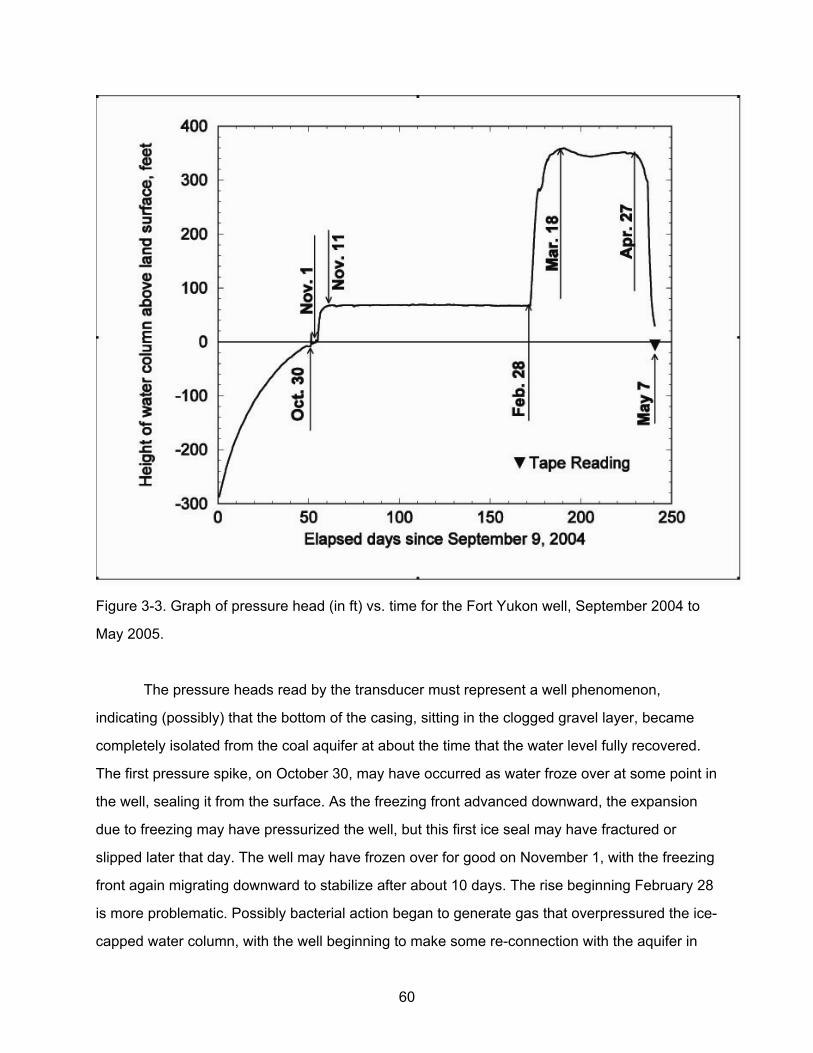
Figure 3-3. Graph of pressure head (in ft) vs. time for the Fort Yukon well, September 2004 to

May 2005.

 

The pressure heads read by the transducer must represent a well phenomenon,

indicating (possibly) that the bottom of the casing, sitting in the clogged gravel layer, became

completely isolated from the coal aquifer at about the time that the water level fully recovered.

The first pressure spike, on October 30, may have occurred as water froze over at some point in

the well, sealing it from the surface. As the freezing front advanced downward, the expansion

due to freezing may have pressurized the well, but this first ice seal may have fractured or

slipped later that day. The well may have frozen over for good on November 1, with the freezing

front again migrating downward to stabilize after about 10 days. The rise beginning February 28

is more problematic. Possibly bacterial action began to generate gas that overpressured the ice-

capped water column, with the well beginning to make some re-connection with the aquifer in

60

early May. The pressure clearly was released completely when the ice in the well was thawed.

The above are merely conjectures, and the true cause of the strange well behavior may never

be known. Nonetheless, it is extremely unlikely that the recorded pressure heads represent

those in the formation.

Test 4

Despite these problems, the early data, extending to October 30, appear to represent

recovery from the air-lift pumping on September 8, and will be analyzed as such. Pressure head

was computed as 638 ft (depth of 610 ft+ barometric pressure of 34 ft-6 ft SWL), minus the

transducer reading. H0 of 297 ft, the same as for test 3, is assumed. The resulting plot of 1-H/H0

versus time is a continuation of the data plot for test 3, as it should be. The match points and

determined KD and K values are the same for the two tests. After about 30 days and 80 percent

recovery, the pressure head recovery is more rapid than predicted by slug test theory. The

cause of this is unknown, but has been observed by the authors for a few other slug tests on

coal beds in the Powder River Basin of Montana and in central Alaska.  

Summary of Aquifer Test Analyses

In summary, the testing regime for this well was fraught with difficulties and

uncertainties. Development of the well was in progress when the casing slipped 35 ft, precluding

an extensive test on the fully developed well open to 48 ft of coal. Depressuring for the second

test led to a cave-in of the well, further reducing its production capacity and effective KD.

Despite these problems, the resultant slug tests provide a range of values that may bracket the

true hydraulic conductivity or permeability of the coal. The results of matching the data for test 1

to a maximum probable value indicate a minimum K (k) of 6X10-4 ft/d (0.3 mD). The maximum

hydraulic conductivity is less easily obtained. A 1-in. thick clogged layer that is 100 times less

permeable than the coal would result in a computed K (k) of about 6X10-3 ft/d (3 mD). Such a

permeability reduction is within the realm of possibility, but may overstate conditions for test 1. A

good estimate of the permeability of the coal at this site, based on reasonable agreement of k

values for tests 1 and 2, may be about 0.6 mD. This permeability is lower than that determined

from aquifer tests and slug tests conducted on several coal beds by the authors in the Powder

River Basin in Montana, but is not anomalously low compared to k values for coal beds in the

61

San Juan and Black Warrior Basins (McKee and others, 1988). Coal bed methane development

in those basins is accomplished by extensive hydraulic fracturing of the coal beds (Zuber, 1996,

p. 3.18–3.19), a practice that almost certainly will be required for the development of coal bed

methane at Fort Yukon.

The relatively low methane content and low permeabiliity of the coal indicate that the

potential for methane development at Fort Yukon is limited, and plans for a multiple well aquifer

test were abandoned. The well was plugged and abandoned following retrieval of the

transducers, temperature logging, and water sampling in May 2005.

Water Chemistry Analyses 

The water-chemistry analyses related to the upper coal bed are based on 3 water

samples, two from the well and one from a core sample. Sample Well_1 was captured during

air-lift development of the coal from a depth of about 1,300 ft and sample Well_2 was bailed

from this same depth after the well was thawed in May 2005. The siltstone sample was

obtained by squeezing a core sample collected from a depth of 1,400 ft, 55 ft below the bottom

of the upper coal zone. For comparison, two samples of surface water used in the drilling

operation (Truck A and Truck B) were also analyzed to ensure that the water samples from the

well were not affected by the drilling fluids.

Unfiltered samples were refrigerated after collection prior to returning them to the USGS

laboratory in Lakewood, Colo. At the laboratory, the samples were filtered through a 0.45 mm

filter and the sample for cations was acidified to a pH of less than 2. Cations were analyzed by

standard inductively-coupled plasma emission spectroscopy (ICP_AES) and anions were

determined by standard ion chromatography. Tables 3-4A and 3-4B give the composition of

major ions and selected trace elements respectively. The data on water quality presented here

should be viewed as qualitative only because of the lack of stringent sampling and collection

protocols.

The 3 samples from the coal and siltstone are Na-HCO3 type waters with total dissolved

solids (TDS) ranging from 880 to 1,480 mg/L, and display the dominant characteristics of typical

CBM waters: sodium and bicarbonate as dominant cation and anion, low sulfate values, implied

62

low redox potential, and high sodium adsorption ratio1 (SAR) (Table 3-4A). This similarity is

demonstrated in fig. 3-4, which compares the analyses with those for a large suite of water

samples collected from methane-bearing coal beds in the Powder River Basin, Wyoming and

Montana (Rice and others, 2002). Surprisingly, the siltstone sample most closely resembles

CBM water typified from the Powder River Basin (fig. 3-4). The sulfate value is very low (<10

mg/L), and, because of the low sulfate value, the Ba++ value is high (4.7 mg/L). The high Fe

concentration suggests that the water was reducing, also consistent with typical CBM produced

waters. The biogeochemical processes that produce water typical of CBM developments are

discussed by Rice and others (2002) and by Van Voast (2003).

The samples collected from the coal and siltstone are distinctly different in both

composition and TDS compared to the truck samples, which are representative of water used to

drill the well (fig. 3-4, table 3-4A). The truck samples represent a low TDS (<400 mg/L) Ca-Mg-

SO4-HCO3 type water with low concentrations of Na (<20 mg/L), small SAR values (<1), and

major anions comprising both sulfate and bicarbonate. Lack of a discernible mixing trend

between the well samples and the truck samples (fig. 3-4) indicates that contamination of the

formation water samples by drilling fluid is minimal.

The water chemistry data suggest that problems associated with the disposal of water

co-produced with methane from the upper coal bed would be minimal. Total dissolved solids for

the formation waters are somewhat, but not drastically higher, than the primary drinking water

standard of 500 mg/L, and the SAR is high enough that the water might not be suitable for

irrigation applications, an unlikely use of the water. Trace elements for the well samples are

below drinking water standard criteria, but those squeezed from the siltstone for Fe, Ba, and Al

are above them. A final determination of needed disposal practices, assuming methane

development was implemented, would require additional water quality sampling and analysis.

63

1 2/][ MgCaNaSAR , where concentrations are in milliequivalents.

Table 3‐4A. Concentrations of major ions in water samples from drill hole DOI‐04‐1A, Fort Yukon, Alaska.  The concentration of HCO3 is estimated from charge balance and represents total alkalinity. 

  CO   O   PO Sample  TDS  Na  Ca  Mg  SAR  K  Cl  SO4 H 3 N 3 4 

mg/L  mg/L  mg/L  mg/L    mg/L  mg/L  mg/L  mg/L  mg/L  mg/L Well_1   978  310  37  27   9.45  20.0  12  130   900  bdl  bdl Well_2   881  280  24  11  11.87  17.0  14  210   660  4  1.9 Siltstone  1478  430  55  75   8.85  45.0  25    8  1710  bdl  bdl Truck_A   390   15  45  55   0.35   4.1  14  120   280  bdl  bdl Truck_B   323   12  23  52   0.32   4.3  13  120   200  bdl  bdl 

Abbreviations: mg/L, milligrams per liter; bdl, below detection limit 

 Table 3‐4 . Concentrations of selected trace elements in water samples from drill hole DOI‐04‐1A, Fort Yukon, Alaska. B

Sample 

Si  Al  Fe  Mn  Ba  Sr  Zn  mg/L  g/L  g/L  g/L  g/L  g/L  g/L Well_1  4.4  110   58  110  430  290  120 Well_2  na  na   90  na  110  390  Na Siltstone     25  7100    1580  <60    4700  820  480 Truck _A  9.4  1150    <250    87  100  210  290 Truck_ B  3.4  <625    <250  <60   92  190  270 

Abbreviations: mg/L, milligrams per liter; g/L, micrograms per liter 

 

64

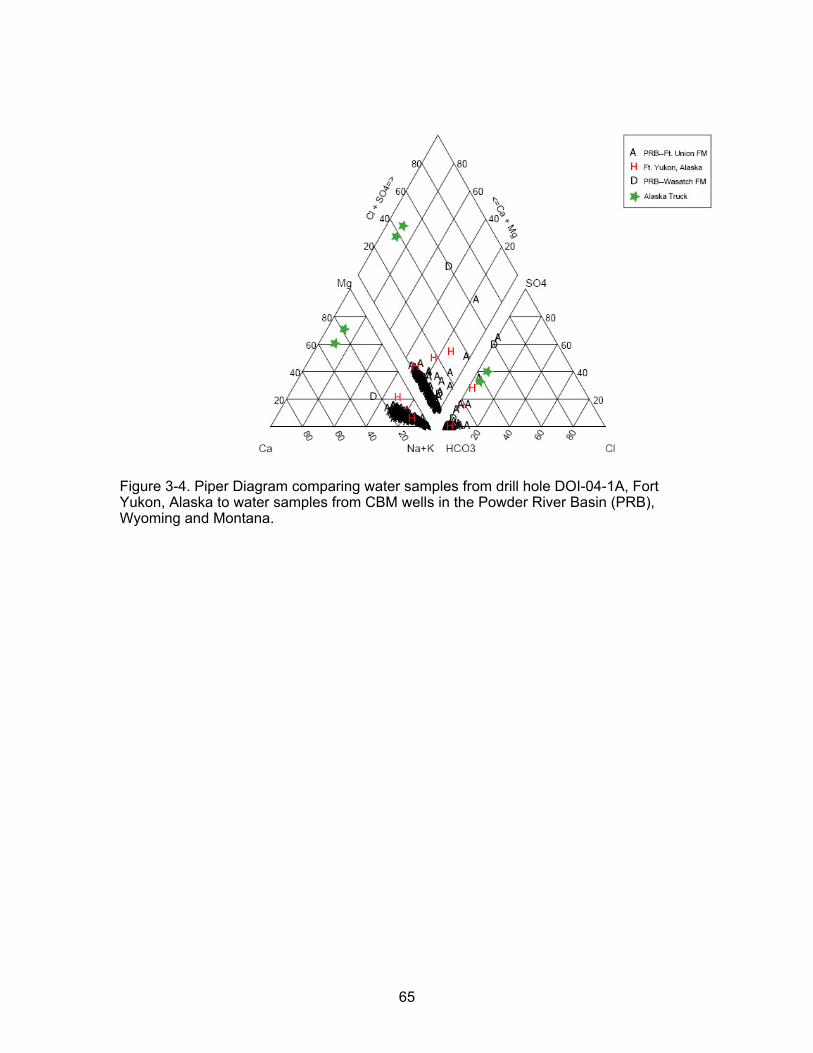
 Figure 3-4. Piper Diagram comparing water samples from drill hole DOI-04-1A, Fort Yukon, Alaska to water samples from CBM wells in the Powder River Basin (PRB), Wyoming and Montana.

65

References Butler, J.J., 1997, The design, performance, and analysis of slug tests: Lewis, Boca

Raton, Florida, 252 p.

Cooper, H.H., Bredehoeft, J.D., and Papadopulos, I.S., 1967, Response of a finite-

diameter well to an instantaneous charge of water: Water Resources Research, v. 3 no. 1, p. 263–269.

Earlougher, R.C. Jr., 1977, Advances in well test analysis: Society of Petroleum

Engineers Monograph, v. 5, 264 p.

Greene, E.A., and Shapiro, A.M., 1995, Methods of conducting air-pressurized slug tests

and computation of type curves for estimating transmissivity and storativity: U.S. Geological Survey Open-File Report 95–424, 43 p.

Matthews, C.S., and Russell, D.G., 1967, Pressure buildup and flow tests in wells:

Society of Petroleum Engineers Monograph, v. 1, 167 p. McKee, C.R., Bumb, A.C., and Koenig, R.A., 1988, Stress-dependent permeability and

porosity of coal and other geologic formations: SPE Formation Evaluation, v. 3, no. 1, p. 81–91.

Rice, C.A., Bartos, T.T., and Ellis, M.S., 2002, Chemical and isotopic composition of

water in the Fort Union and Wasatch Formations of the Powder River Basin, Wyoming and Montana: Implications for coalbed methane development, in Schwochow, S.D., and Nuccio, V. F., eds., Coalbed Methane of North America, II: Rocky Mountain Association of Geologists, p. 53–70.

Van Voast, W.A., 2003, Geochemical signature of formation waters associated with

coalbed methane: American Association of Petroleum Geologists Bulletin, v. 87, p. 667–676.

Weeks, E.P., 2005, Hydrologic properties of coal beds in the Powder River Basin,

Montana II. Aquifer test analysis: Journal of Hydrology, v. 308, p. 242–257.

Zuber, M.D., 1996, Basic reservoir engineering for coal, in Saulsberry, J.L., Schafer,

P.S., and Shraufnagel, R.A., eds., A Guide to Coalbed Methane Reservoir Engineering: Gas Research Institute, Chicago. Ill., variously paginated.

66

Summary of Results:

Coalbed Methane Production Potential in Fort Yukon, Alaska as Derived from the DOI-04-1A Well

By Edwin P. Weeks1, Arthur Clark2, and Charles E. Barker3

Fort Yukon Production Potential

The permeability estimates provided for the upper coal bed in table 3-3, assumed

to also apply to the lower coal, may be used in conjunction with the methane desorption

data (tables 2-1A, 2-1B) and adsorption isotherms (figs. 2-1, 2-2), to roughly evaluate

the potential for methane production at Fort Yukon. In particular, the results can be used

to estimate the number of wells and well spacing required to produce 225,000 standard

cubic feet of pure methane per day (scf/d), the estimated requirement for power

generation and home heating at Fort Yukon (Ferguson and Ogbe, 2003, p. 14).

An absolute control on coalbed methane availability is imposed by the volume of

gas initially in place per unit area. Volumetric gas in place can be determined from the

equation: , where IGIP is initial gas in place, Mscf/acre; 1.359 is a

conversion factor, [(Mscf)(ton)(cm3)]/[(ac-ft)(scf)(gm)]; C is average as-received gas

content of the coal, scf/ton; c is mean raw coal density, g/cm3; h is coal bed thickness,

ft; and is the mole fraction of methane in the desorbed gas. For the upper coal, C=13.1

hCIGIP c359.1

scf/ton (table 2-1A), c=1.34 g/cm3 (table 2-2A), h= 59 feet, and =0.94, resulting in

IGIP=1.3 MMscf methane/acre. For the lower coal, the average gas content of 19.1

scf/ton (table 2-1B), coal density of 1.48 g/cm3 (table 2-2B), combined with a coal

______________________________________________________________________________________________________________

1 Corresponding author, U.S. Geological Survey, Denver, Colo. phone: (303) 236-4981 epweeks@usgs.gov 2 U.S. Geological Survey, Denver, Colo. 3 Scientist Emeritus, U.S. Geological Survey, Denver, Colo.

67

thickness of 20 ft, results in IGIP of about 700 Mscf/acre.

For a pure methane fuel requirement for the village of 225 Mscf/d or 80 MMscf/yr,

the village would require 1.6 billion scf over a 20-year period. Assuming a 100 percent

recovery efficiency, all of the gas, if derived from the upper coal, would have to be

removed from an area of about 1,200 acres, or, if dual completion of wells tapping the

two zones is feasibile, could be obtained from a 800-acre area. However, complete gas

recovery is not possible, and a rigorous evaluation of the 20-year recovery efficiency

would require reservoir simulation, which is beyond the scope of this study. Nonetheless,

a rough estimate of the number of wells needed to supply the village energy

requirements may be obtained by analogy with results of simulations performed to

evaluate recovery efficencies based on San Juan Basin coal properties. Zuber (1996, p.

3.18–3.19) provides illustrations for well spacings of 80, 160, and 320 acres, showing

simulated 20-year recovery efficiencies vs. permeability and hydraulic fracture length for

San Juan Basin coals. Zuber’s curves indicate that computed recovery efficiency is

nearly zero without hydrofracing for permeabilities less than 1 millidarcy, but increases

sharply with diminishing well spacing and with stimulated fracture length.

Simulated efficiencies undoubtedly would be smaller for the low level of methane

saturation for the Fort Yukon coals than those derived for methane-rich San Juan Basin

coals. Nonetheless, estimates of the minimum number of hydrofraced vertical wells

needed to meet the requirements can be made from recovery efficiencies illustrated in

these figures, test-based permeability estimates, and the IGIP estimates. For the

preferred estimate of coal permeability of 0.6 mD (table 3-3), the simulated curves for a

spacing of 80 acres and an arbitrarily chosen stimulated fracture length of 200 ft

(Zuber,1996, p. 3.18) indicate a 20-year recovery efficiency of about 30 percent. Based

on this efficiency, about 50 wells tapping the upper coal, covering an area of 4,000

acres, would be required to meet village needs. For dual completion in the upper and

lower coals, but the same recovery efficiency, about 30 wells in an area of 2,700 acres

would be required. Zuber’s curves also indicate that, for a given fracture length, recovery

efficiency increases, at low K values, by about 12 percent for each halving of well

spacing. Thus, 20-year recovery efficiency might be about 42 percent for a 40-acre

68

69

spacing, indicating that about 50 dual-completion wells covering about 2,000 acres might

be able to meet the village requirements.

Recent developments involving the use of horizontal wells indicates that the

number of wells required might be decreased by a factor of three to five or more,

reducing the number of wells required to as few as 5 to 10. However, the actual

feasibility of developing the Fort Yukon coals using dual-completion hydrofraced

horizontal wells would require thorough evaluation using a reservoir model. The above

analyses only provide a basis for indicating whether such a study might be useful.

References:

Ferguson, J.C., and Ogbe, D.O., 2003, Fuel gas utilization and economic study:

Application to Fort Yukon, Alaska: Petroleum Development Laboratory, University of

Alaska, Fairbanks, 17 p.

Zuber, M.D., 1996, Basic reservoir engineering for coal in Saulsberry, J.L., Schafer,

P.S., and Shraufnagel, R.A., eds., A Guide to Coalbed Methane Reservoir

Engineering: Gas Research Institute, Chicago Ill., variously paginated.