DRAFT WORKING PAPER

1

Explaining nationalist political views: The case of Donald Trump

Jonathan Rothwell

Senior Economist, Gallup

Last revised August 1, 2016

Abstract

The 2016 US presidential nominee Donald Trump has broken with the policies of previous

Republican Party presidents on trade, immigration, and war, in favor of a more nationalist and

populist platform. Using detailed Gallup survey data for a large number of American adults, I

analyze the individual and geographic factors that predict a higher probability of viewing Trump

favorably and contrast the results with those found for other candidates. The results show mixed

evidence that economic distress has motivated Trump support. His supporters are less

educated and more likely to work in blue collar occupations, but they earn relative high

household incomes, and living in areas more exposed to trade or immigration does not increase

Trump support. There is stronger evidence that racial isolation and less strictly economic

measures of social status, namely health and intergenerational mobility, are robustly predictive

of more favorable views toward Trump, and these factors predict support for him but not other

Republican presidential candidates.

DRAFT WORKING PAPER

2

Introduction

The 2016 Republican Party presidential nominee in the United States is Donald Trump, a man

who has based his campaign largely on restricting immigration, in part by building a large wall

along the border with Mexico and barring Muslims from entering the country, and restricting

trade, by re-negotiating trade agreements and imposing tariffs on China and possibly other

countries.1 His first foray into national polictics created headlines by accusing President Barak

Obama of having conspired to forge his US-based birth certificate, despite the insistence of

state officials from Hawaii that he was born there and they still have his birth certificate on

record.2 With these positions and others, including his criticism of former president George W.

Bush and the Iraq War, Trump’s candidacy has attracted the support of right-wing nationalists,

and provoked criticism from Republican party media and political leaders.3

This article examines the characterisics of Trump’s supporters with a view to establishing

broader insight into what factors motivate nationalist political identification. Trump’s nationalist

appeals were evident in his acceptance speech of the Republican Party’s nomination:

“The most important difference between our plan and that of our opponents, is that our plan will put America First. Americanism, not globalism, will be our credo. As long as we are led by politicians who will not put America First, then we can be assured that other nations will not treat America with respect. This will all change in 2017. The American People will come first once again.”4

There is a large literature on historic and contemporary nationalist or nativist parities in Europe

(Muddle 2007). In a study of perhaps the most infamous party, the geogrpahy of voting patters

reveal that the political supporters of Hitler’s National Socialist party were largely comprised of

rural Protestants and of the non-farm population those in lower-middle class administrtive

occupations or working class occupations, likely with much education than their counterparts

(Hamilton 2014).

In work closely related to this project, Mansfield and Mutz (2009) find that ethnocentrist and

islationist world-views predict opposition to free trade, and after accounting for these factors,

invididual economic characteristics such as education are not signfiicant. In a similar analysis,

but of support for outsourcing, Mansfield and Mutz (2013) find that nationalism, ethnocentristm,

and isolationism predict opposition to outsourcing, but objective econmic threat—in terms of

occupational or industrial employment—does not. The implication of these studies that is that

rational self-interest is less relevant to political preferences than nationalist and related attitudes.

Quite recently, the 2016 “Brexit” referendum, in which a majority of UK voters decided to leave

the European Union, revealed stark divisions at small geographic units. Local authority areas

1 See campaign website, https://www.donaldjtrump.com/positions; Reinhard, B and Paletta, D. “Donald

Trump Back-Pedals on Banning Muslims From U.S.” Wall Street Journal June 28, 2016. 2 Garret Epps, Trump’s Birther Libel, The Atlantic, February 26, 2016. 3 Taub, A. The rise of American authoritarianism, Vox March 1, 2016, available at

http://www.vox.com/2016/3/1/11127424/trump-authoritarianism#fear 4 Donald J Trump, Republican National Convention speech, Jul 21, 2016, available at, http://www.politico.com/story/2016/07/full-transcript-donald-trump-nomination-acceptance-speech-at-rnc-225974#ixzz4FiNnOL3l

DRAFT WORKING PAPER

3

with the following characteristics tended to vote to leave: less post-secondary educational

attainment, lower test scores, older residents, with fewer immigrants and lower incomes.5

Yet, there is scant empirical literature explaining why people support extreme political views

generally and right-wing nationalism in particular. A small body of research likens the rise of

more extreme politics in the United States “(political polarization”) to shocks from import

competition (Autor, Dorn, Hanson, and Majlesi 2016) or income inequality (McCarth, Rosenthal,

and Poole 2006), though neither study considers nationalist political views akin to Trump’s

“America first” rhetoric and proposals.

Even if income or other standard economic measures are not especially helpful in explaining

nationalism, ill-health and cultural behaviors and attitudes may be more revealing. Beyond

standard economic measures, there is evidence that whites are unusually pessimistic about

their well-being, after adjusting for other factors (Graham forthcoming). Specifically, lower-

income whites and older whites exhibit this pessimism compared to other groups (ibid).6 Along

these lines, middle-aged whites have experienced a rise in mortality rates in the last decade and

a half (Case and Deaton 2015).

Additionally, there is a large body of theoretical and empirical literature explaining the conditions

of inter-group conflict. In the early 20th century, research on the military, policing, and public

housing found that inter-group conflict reduced prejudice toward African-Americans (Pettigrew

and Tropp 2006; 2011). The American pyshcologist Gordon Allport (1954) is credited with

establishing this theory in the social science literature, and he further stipulated that contact

reduces prejudice when certain conditions are met: equal status between groups; cooperatively

working toward common goals, and under the support of an external authority (Pettigrew and

Tropp 2006; 2011).

Since, then a large literature has confirmed Allport’s theory, and even found that the conditions

do not necessarily need to be present, at least in modern settings, in which formal civil right

laws have already been established (Pettigrew and Tropp 2006). At the personal level, one

recent study finds that friendly contact with other groups reduces anxiety around the threat of

rejection and eases comfort with physical and conversational engagement (Barlow et al 2009).

At the scale of metropolitan areas, Rothwell (2012) finds that racial segregation but not diversity

predicts lower levels of social capital, measured by trust and volunteering, in the United States.

In so far as nationalist political attitudes are characterized by suspicion of ethnic outsiders,

contact theory would predict less support for nationalist poltical parties. In a direct test of that

hypothesis, Biggs and Knauss (2012) find that neighborhood level exposure to minorities

predicts lower membership rates in British nationalist parities. These neighborhood level

correlations would be biased if people sort into neighborhoods based on political preferences,

but Kaufmann and Harris (2015) finds no evidence of geographic sorting based on nationalist

political views. In related work, Jorgen Soreson (2014) finds that an initial wave of immigration

5 The Guardian, “EU Referendum Results and Full Analysis,” accessed July 29, 2016, available at http://www.theguardian.com/politics/ng-interactive/2016/jun/23/eu-referendum-live-results-and-analysis 6 See Chapter 4 of Graham (forthcoming), which shows regressions of anticipated life satisfaction in five-years on dummy variables for race interacted with income (Table 4.2a) and age (Table 4.2b). The black and Hispanic coefficients are significant and positive by themselves (relative to whites) and significant and positive when interacted with low income status or age for blacks and Asians.

DRAFT WORKING PAPER

4

at the local level increased support for a right-wing party in Norway, but the effect quickly faded

out, which the author suggests is the result of direct contact with immigrants.

This analysis attempts to explain the characteristics of Trump supporters and test two

hypotheses:

1. Social hardship increases the likelihood of Trump support

2. Contact with immigrants or racial minorities reduces the likelihood of Trump support

3. Exposure to trade competition increases support for Trump

For the first, I distinguish between traditional measures of economic hardship like income and

employment status in favor of measures of health and intergenerational mobility. The former is a

core component of well-being, and the latter may be related to one’s hope for the furture well-

being of offspring, which may, in turn, directly affect personal well-being and level of satisfaction

with the political status quo.

To test the second hypothesis, I analyze the degree of neighborhood segregation and distance

to the Mexican border, and for the third, I predict how support for Trump varies by the share of

employment in the manufacturing sector, as well as various other measures as robustness

checks.

The paper proceeds with a description of the data and methods, a summary of the ideological

differences between Trump supporters and other groups, particularly other Republicans, and a

broader summary of the microdata used. The empircal section highlights the individual and

geogrpahic correlaries of Trump support, in light of the hypothesis desribed above. The

discussion concludes with an effort to situate these findings in a larger theoretical context.

Data and analysis

The main data are Gallup Daily Tracking survey microdata, collected from July 8, 2015 through

July 25, 2016. 93,207 American adults were asked if they hold a favorable view of Donald

Trump over this period. Of these, 87,428 responsed either yes or no (with 65% reporting an

unfavorable view). 4% reported no opinion, 1% percent said they hadn’t heard of him, and less

than one percent refused to answer. The analysis discards observations from those who did not

answer yes or no. Survey weights developed by Gallup methodologists were applied to make

the sample size nationally representative. This is a very large sample size relative to the two

thousand or less used in comparable studies (eg Mansield and Matz 2009, 2013).

The principal method used is multi-variable probit regression, designed to estimate how various

factors are associated with the binary probability of holding a favorable view of Trump in

Gallup’s Daily Tracking surveys. The data were collected from July 8, 2015 to July 25, 2016 and

Trump favorability could be analyzed for 87,428 observations, in which a respondent answered

either favorable or unfavorable. Those who did not know or refused were excluded from this

analysis.

A county level indicator from the Gallup surveys was linked to CZs using a county-CZ crosswalk

developed by David Dorn and made available on his personal website. Zip-code level data from

the US Census was linked to Gallup survey data, which contains zip codes, by converting zip

DRAFT WORKING PAPER

5

code tabulation areas (ZCTAs) to traditional zip codes using a crosswalk funded by the US

Health Resources and Service Administration.7

Equation one shows the basic model.

1. 𝑃 [𝑇𝑖,𝑐] = 𝐼𝑖,𝑐 + 𝐶𝑐 + 𝜀𝑖,𝑐

The probability of individial i residing in commuting zone c of holding a favorable view of Trump

is modelled as a funciton of a vector of individual characteristics (I) and commuting zone

characteristics (C). The residual is assumed to have both an individual and commuting zone

component, and errors are clustered at the commuting zone level to account for within CZ

correlations. Sample weights are also applied to make the analysis representative at the

national level. The analysis also includes the date of the interview to account for the fact that

voters may have changed their views based on the candidates performance during the primary

elections and campaign. This basic set up will also be repeated to mesaure favorability toward

other candidates to compare the results against Trump.

The I term contains various demogrpahic measures, shown below, and the C term examines:

distance to the Mexican border;

the manufacturing share of employment;

intergeneratinal mobility

racial segregation;

mortality rates

educational attainment

population

Distance to Mexico was calculated by first allocating the centroid longitude and latitude

coordinates for the largest county by 2010 population to each commuting zone, using data from

American Fact Finder and the 2010 Decennial Census. Second, distance between these CZs

and the Mexican border was approximated by grouping CZs into longitudinal regions and

calculating their distance to one of five border MSAs using the “vincenty” command in STATA,

based on their longitude: San Diego, for the westernmost CZs with longitudinal coordinates less

than -115.345; Yuma (-115.3 to -112.8); Tucson (-112.8 to -109.0); El Paso (-109.0 to -102.2);

McAllen (>-102.2).

The manufacturing share of employment is calculated using data from the QCEW. Since data

suppressions are present in even the high level data file, the analysis is supplemented using

manufacturing and other employment level estimates from Acemoglu et al (2016). They

developed a method to impute over County Business Patterns data suppressions and have

made their data available. The analysis also uses an index of Chinese import exposure from

Autor, Dorn, and Hanson (2013).

To measure potential political preferences stemming from a lack of inter-generatioanl mobility,

the analysis uses a measure of intergenerational mobility at the CZ level from Chetty et al

(2014), which they constructed using an Internal Revenue Service database of all federal tax

records for individuals born between 1980 and 1982, which they linked to the tax records of their

parents. Intergenerational mobility is caluclated as the average CZ national income rank at age

7 UDS Mapper, Zip Code to ZCTA Crosswalk, available at http://udsmapper.org/zcta-crosswalk.cfm

DRAFT WORKING PAPER

6

30, for individuals raised at the 25th percentile of the national income distribution, using family

income between ages 15 and 20. Chetty and Hendren (2015) subsequently developed a

method to estimate the causal effect of a commuting zone on intergenerational mobility, to

eliminate effects from migration. This causal effect on intergenerational mobiltiy is the preferrred

variable for this analysis, because it filters out local migratory effects.

Racial segregation in this anlaysis is measured by matching survey respondent zip codes to

census population data (originally from ZCTAs) from the 2010-2014 5-year Ameican Community

Survey. Segregation is measured in two ways.The first uses the difference in the white share of

population at the zip code and CZ levels. The second uses the ratio of CZ diversity to zip code

diversity, using standard diversity index measures.

1. Racial isoaltion of whites = zip code share white – CZ share white

2. 𝑅𝑎𝑐𝑖𝑎𝑙 𝑖𝑠𝑜𝑙𝑎𝑡𝑖𝑜𝑛 =Diversity index CZ

Diversity index zip

𝑤ℎ𝑒𝑟𝑒𝑏𝑦 𝐷𝑖𝑣𝑒𝑟𝑠𝑖𝑡𝑦 𝑖𝑛𝑑𝑒𝑥 = 1 − ∑(𝑝𝑔2)

For both, higher values indicate greater segregation. The overall white share of the CZ

population is included as a control variable in the first and overal CZ diversity is included as a

control in the second.

Health status for likely Trump supporters is mesaured using the 2014 mortality rate for white

non-hispanics aged 45 to 54. These data are from the US Centers for Disease Control (CDC

Wonder). County level total deaths and population were aggregated to the CZ level. All causes

of death were included. To supplement the analysis, data from Chetty et al (2016) are included

to mesaure life expectancy at birth at various income levels for the entire CZ population.

CZ level population and educational attianment data are calcualted from county data available

from the 2010-2014 American Community Survey.

Any analysis looking at support for a particular politician raises the issue of whether the results

are attributable to the party or the specific characteristics of the politician and his or her

positions. There are also possible interaction effects between the various independent variables

and race and party affiliation. To account for this, the regression models are estimated against

three samples: the entire sample, a sample of all white non-Hispanics, and a sample of white

non-Hispanic Republican party members. To identify the latter, a Gallup survey question (“As of

today, do you lean more . . .”) is used, whereby those who lean Republican or simply choose

Republican are coded as Republican-party affiliated.

Evidence that Trump supporters differ from other Republicans

To start, it is worth noting where Donald Trump’s supporters identify themselves on the

ideological spectrum. The evidence suggest Trump’s supporters are significantly further to the

right than even other Republicans. The Gallup Daily Tracker asks respondents to “desribe your

political views” and provides options of very conservative, conservative, moderate, liberal, or

very liberal. As shown in Table 1, those who view Trump favorbably are significantly more likely

to identify as conversative or very conservative compared to those who do not. Of greater

DRAFT WORKING PAPER

7

interest, is the comparison between columns 3 and 4, which compare those who view Trump

favorably to those who do not among only Republicans. The differences on very conservative (4

percentage points) are highly significant, with Trump supporters being further right. The total

conservate share difference (12 percentage points) is also highly significant.

In addition to broad ideological orientation, Republicans who favor Trump are also significantly

more likely than other Republicans to oppose trade and immigration. The Gallup Daily Tracker

reserves some space for topical questions asked for bried periods of time. One question asks

whether or not the respondent agrees or disagrees with the statement “End U.S. participation in

free trade deals, such as NAFTA” and another states “Reform immigration laws to provide

automatic green cards for high skilled workers” Among Republicans who favor, 58 percent

oppose trade deals and 57 percent oppose reforming immigration. By contrast, among

Republicans who do not support Trump, 42 percent oppose trade deals and 28 percent oppose

reforming immigration laws.

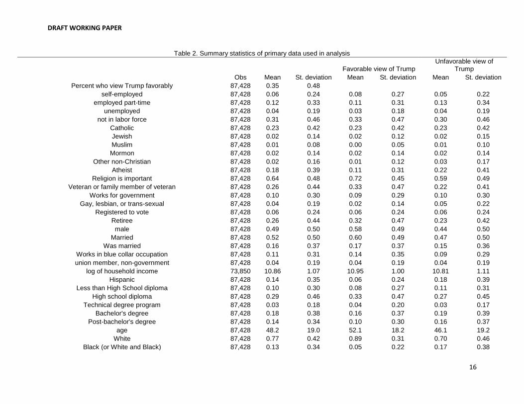
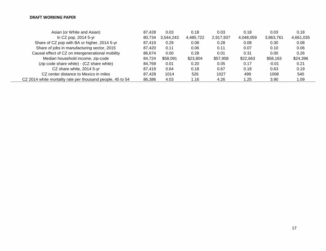
Summary data

The means and standard deviations of the full database used here, including the CZ level

variables, is provided in Table 2. Trump’s supporters are older, with higher household incomes,

are more likely to be male, white non-Hispanic, less likely to identify as LGBTQ, less likely to

hold a bachelor’s degree or higher education, more liekly to be a verteran or family member of a

veteran, more likely to work in a blue-collar occupation, and are more likely to be Christian and

report that religion is important to them. Those who view Trump favorbaly are slightly less likely

to be unemployed and more likely to be self-employed. Labor force participation is lower among

Trump supporters, but not after adjusting for age. Trump supporters are much more likely to be

retired. Trump supporters live in smaller commuting zones with lower college attainment rates, a

somewhat higher share of jobs in manufacturing, higher mortality rates for middle-aged whites,

and a higher segregation. There is no statistically significant difference between Trump

supporters and non-supporters with respect to the median household income of their zip-code, a

proxy for neighborhood conditions.

The next section will examine the marginal contributions of individual level variables in

predicting Trump support, while holding other factors constant, and then turn to variables

measured at higher levels of geograph to observe how zip code and CZ level variables affect

the probability of supporting Trump, conditional on those individual factors.

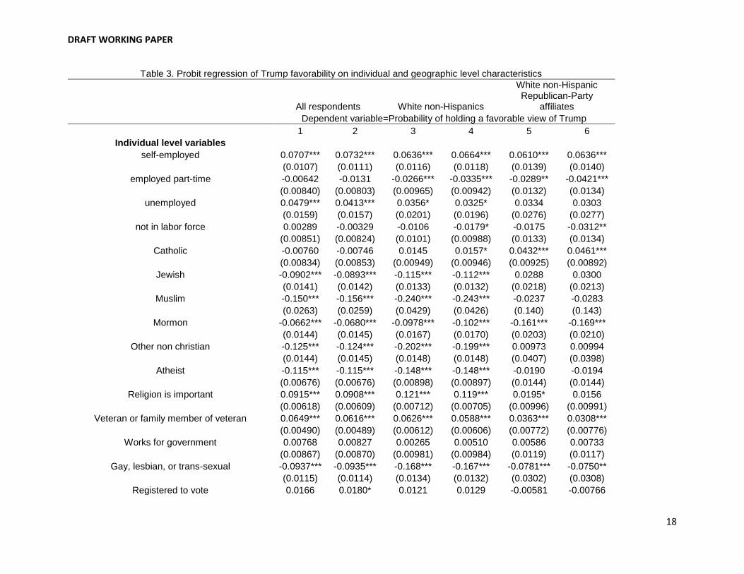
Results for individual correlates

The main results from the probit regressions are reported below in Table 1. Columns one and

two use the entire survey sample but differ in their measures of segregation. Column one uses

the difference in the white share of population at the zip code and CZ levels, whereas column

two uses CZ diversity relative to zip code diversity. Columns three and four limit the sample to

non-Hispanic whites, wheres columns 5-6 limit the respondents to Republican-Party affiliated

non-Hispanic whites. This is done to distinguish between Trump support and Republican

support more generally.

The individual data do not suggest that those who view Trump favorable are confronting

abnormally high economic distress, by conventional measures of employment and income.

DRAFT WORKING PAPER

8

Controlling for a variety of demographic and geographic characteristics, Trump supporters are

more likely to be self-employed, overall and among other whites, and other white Republicans,

somewhat more likely to be unemployed overall but not among other whites or white

Republicans, and no more likely to be out of the labor force compared to any group.

Higher household income predicts a greater likelihood of Trump support overall and among

whites, though not among white non-Hispanic Republicans. In other words, compared to all non-

supporters or even other whites, Trump supporters earn more than non-suppporters, conditional

on these factors, but this is partly because Republicans, in general, earn higher incomes, and

the difference is no-longer significant when restricted to this group. The measure of household

income reported imputes the mid-point of income brackets that respondents identifed

themselves as being in.

Using an alternative mesaure of income, suggests Trump supporters earn more than even other

white non-Hispanic Republicans, conditional on education and other factors. The alternative

income measures imputes within self-reported brackets using the median incomes of people in

the same state, income bracket, and age group, based on data from the IPUMS-CPS 2015

Annual Social and Economic Supplement. Trump supporters earn significantly higher household

incomes in all segments using the CPS-imputed data.

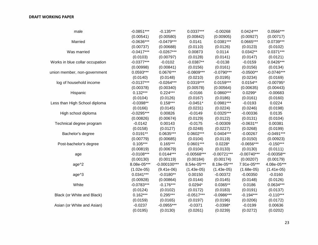
On the other hand, workers in blue collar occupations (defined as production, construction,

installation, maintenance, and repair, or transporation) are far more likely to support Trump, as

are those with less education. People with graduate degrees are particularly unlikely to view

Trump favorably. Since blue collar and less educated workers have faced greater economic

distress in recent years, this provides some evidence that economic hardship and lower-socio-

economic status boost Trump’s popularity.

Still, Hispanics and blacks are roughly 20 percentage points less likely to view Trump favorably

than non-Hispanic, even controlling for income, education, and many other variables. This is

strong evidence that economic factors alone cannot account for his support. 14 percent of

blacks and Hispanic adults view Trump favorably, and this rises to just 16 percent among black

and Hispanics working in blue collar occupations, a statisically significant but very small

difference.

Results for higher geographic correlates

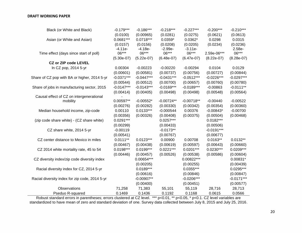
Segregation, mortality, distance to Mexico, and lower college education shares are all robustly

predictive of Trump support across these samples. Exposure to manufacturing tends to predict

significantly lower Trump support. (All CZ level variables are standardized to faciliate

comparisions of effect sizes, and the results are reported at the bottom of Table 1).

People living in zip codes with disproportionately high shares of white residents are significantly

and robustly more likely to view Trump favorably. A one standard deviation in the racial isoaltion

index predicts a 2.9 percentage point increase in Trump’s popularity. This holds among white

non-Hispanics and white-non Hispanic Republicans, though the strength of the relationship falls

to 1.8 percentage points.

Those living in zip codes with overall diversity that is low relative to their commuting zone are

also far more likely to view Trump favorably. This holds acorss samples, though unlike white

racial isoaltion, it is not significant among white non-Hispanic republicans. However, a simple

DRAFT WORKING PAPER

9

mesaure of racial diversity at the zip code level predicts lower support for Trump even among

this group and in the larger samples as well.

These results provide strong support for contact theory, and they are bolstered further by the

strong relationship between distance to Mexico and support for Trump. A standard deviation in

distance to the Mexican border predicts a significant 1.1 percent percentage point increase in

the likelihood of viewing Trump favorably in the full sample. This relationship is not significant

among only white non-Hispanics, but interestingly, it becomes significant again for white non-

Hispanic Republicans.

Using distance to Mexico rather than the Hispanic population share has the advantage of removing any endogenous component associated with the economic attraction of Hispanics to a commuting zone. Still, the results are similar using either measure. Replacing the distance measure with the share Hispanic in column one, also predicts significantly lower support for Trump, though not among white non-Hispanic Republicans. The two measures (distance to Mexico and the Hispanic share of the CZ population) are highly correlated ( -0.59), and the correlation is even stronger between the Mexican-born population share and distance to Mexico (-.73). Using distance to Mexico as an instrumental variable for the Hispanic population share also yields significant effects for the entire sample and the white non-Hispanic Republican sample.8

At the individual level, there was little clear evidence that economic hardship predicts support for

Trump, in that higher household incomes tend to predict higher Trump support. Yet, at the CZ

level, two alternative measures of living standards—health and intergenerational mobility—

provide support for the idea that Trump supporters are less prosperous than others.

People living in commuting zones with higher white middle-aged mortality rates are much more

likely to view Trump favorably. A one standard deviation in mortality predicts a roughly 2

percentage point increase in favorable views toward Trump. Other mesures of health were

considered, including overall race-adjusted life expectancy, overall mortality rates, and white

age-adjusted mortality rates. Race-adjusted life expectacncy was not significant, but the overall

2014 mortality rate was significantly positive in favor of Trump. White mortality was far more

predictive, however, and middle-aged white mortality had the strongest relationship to Trump

support.

In results not shown, I find that people living in CZs with higher obesity rates and higher shares

of people reporting poor or fair overall health status are significantly more likely to favor Trump,

when they replace the mortality rate. These variables become insignificant when the white

middle-aged mortality rate is included in the model, suggesting the latter is a stronger overall

indicator of poor health.9 The fact that the obesity rate and self-reported health status were not

available for whites only may also explain why they have less explanatory power.

Somewhat related to health and general social well-being, a one standard deviation in the

causal effect of a cz on intergenerational mobility predicts a 0.6 to 0.7 percentage point increase

in favorable views toward Trump. This is a small effect relative to the others, but it is robust

8 These results were not published in tables to conserve space but are available upon request. 9 These data are from the Robert Wood Johnson county health rankings database, available at

http://www.countyhealthrankings.org/

DRAFT WORKING PAPER

10

overall and among non-Hispanic whites. To be clear, this is not meant to suggest that with

undue certaintly that growing up in a place that causes lower social mobilty causes Trump

support. This analysis only identifies the correlation. In any case, it does not provide any

explanatory power among non-Hispanic white Republicans.

The size of the CZ has no significant correlation with Trump views, but the bachelor’s degree

share of the population had a very large and robust correlation. A one standard deviation

increase in the share of people above age 25 with a bachelor’s degree, predicts a 3 to 5

percentage point decrease in support for Trump, depending on which sample is considered.

This suggests that cultural islotion from the college educated may increase sympathy for

nationalist politics.

Turning to trade competition, the 2015 share of CZ employment in manufacturing is negative

and significant across the three samples (ie the full sample, white non-Hispanics, and white

non-Hispanic Republicans) and in five of the six models reported below. This is a suprising

result given the relationship between blue collar employment and Trump support and Trump’s

protectionist campaign platform.

To test the robustness of this relationship to various measures of trade exposure, the analysis

varies the date the manufacturing employment shares are measured, to account for the fact that

many places saw large losses in recent years. Other adjustments to the model include using

changes in the share of jobs in manufacutring, reflecting replacement of manufacturing jobs with

those in other sectors, growth (or loss) rates in the number of manufacturing jobs, and total

employment growth. The results are summarized in Table 2, which re-estimates the main full-

sample models using these alterations.

The main model used 2015 employment shares, but 2000 manufacturing employment shares

also predict significantly lower support for Trump, whether measured by the QCEW or

Acemoglu et al (2015)’s imputation of suppressions in County Business Patterns data. Likewise,

an increase in the share of manufacturing employment from 2000 to 2007 (using data from

Autor, Dorn and Hanson 2013) predicts higher levels of Trump support, which is the opposite of

the hypothesized relationship. Overall manufacturing employment growth from 2000 to 2015

has no effect, controlling for 2015 shares, nor does the change from 1990 to 2007. Total

employment growth predicts greater Trump support, suggesting that people in more

economically properous metropolitan areas are marginally more likely to view him favorably.

Finally, a measure of Chinese import exposure predicts less Trump support, but the

relatsionship is not statistically significant.

To summarize, the evidence is mixed as to how economic hardship affects Trump’s popularity.

It seems that lower social status and material hardship play a role in support for Trump, but not

through the most obvious economic channles of income and employment. The evidence is in

favor of contact theory is quite clear. Racial isoaltion and lack of exposure to Hispanic

immigrants raise the likelihood of Trump support. Meanwhile, Trump support falls as exposure

to trade and immigration incresaes, which is the opposite of the predicted relationship.

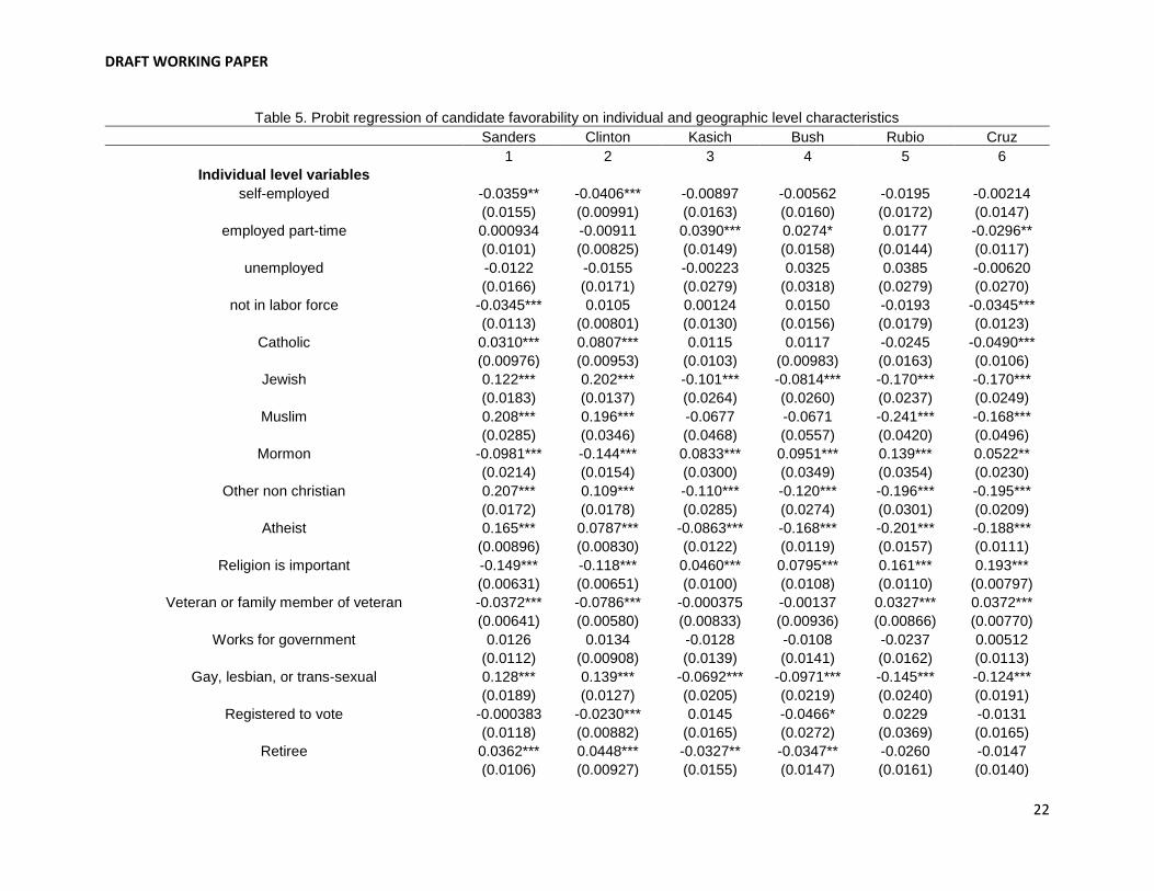
Comparing results across politicians

The analysis shows that Trump supporters standout statistically on a number of dimentions,

even when compared to non-Hispanic white Republicans. In these regresions, the comparison

group consist of white Republicans who do not support Trump, but this does not necessarily

DRAFT WORKING PAPER

11

imply they support other more moderate Republican candidates or Democrats. This section

compares the results from Table 3 column one to other politicians running for the 2016

presidential nomintion in both parties using an otherwise identical model.

Going through the CZ-level resutls, population size had no predictive power for Trump support,

but does predict greater support for Hillary Cliton, John Kasich, and Jeb Bush, who are among

the more moderate candidates. The college attainment rate predicted lower support for Trump,

and this applies more broadly to the other Republican candidates, with the exception of Bush,

where there is no significant correlation. By contrast, more educated areas predict greater

support for Bernie Sanders and Clinton.

Those living in areas with a greater share of jobs in manufacturing were more likely to support

Clinton (the only candidate to hold a positive and significant relationship with this variable).

Aside from Trump, manufacturing orientation was negative and significant only for Bush and

Cruz.

People living in places that cause greater intergenerational mobility are more likely to support

Sanders and Clinton, but there is no effect on other candidates, in contrast to the negative and

significant relationship between mobility and Trump support.

As noted above, those living in aresa with higher white mortality rates are more likely to support

Trump, but are significantly less likely to support Sanders. Interestingly, white mortality had no

relation to support for Clinton or the other Repulican candidates.

As for segregation, Trump once again stands out. Segregation decreases support for Sanders

and, especially, for Clinton, but has no significant predictive power for the other Republican

candidates, though Jeb Bush received significantly lower support in less racially diverse CZs, as

did Hillary Clinton. Distance to Mexico predicts greater support for Sanders, Clinton, and Kasich,

but less support for Cruz, probably because of high support in his home state of Texas. It has

no relation to support for Rubio or Bush.

Some caution is needed in interpreting these results, in that the sample sizes vary across

candidates and are smaller for less popular candidates, particualrly if they dropped out of the

race early, and this will tend to make it less likely to find significant relationships. These patterns

of significance, however, cannot be attrbuted solely to sample size. Some of the other CZ

variables—like population and education—are significant predictors of support for even

candidates with the smallest sample sizes.

In summary, these results confirm that Trump’s supporters differ in important ways from other

Republican candidates. He is the only candidate who recieves significantly more favorable

rating in racially isolated neighborhood and in areas with high middle-aged white mortality rates,

conditional on individual factors. He is also the only candidate for which lower rates of

intergenerational mobility predict greater support.

Discussion

These results do not present a clear picture between social and eocnomic hardship and support

for Trump. The standard economic measures of income and employment status show that, if

anything, more affluent Americans favor Trump, even among white non-Hispanics. Surprisingly,

there appears to be no link whatsoever between exposure to trade competition and support for

nationalist policies in America, as embodied by the Trump campaign.

DRAFT WORKING PAPER

12

Yet, more subtle measures at the commuting zone level provide evidence that social well-being,

measured by longevity and intergenerational mobility, is significantly lower among in the

communities of Trump supporters. The causal mechanisms linking health and intergeneratinal

well-being to political views are not well-understood in the social science literature. It may be the

case that material circumstances caused by economic shocks manifest themselves in

depression, dissapointment, and ill-health, and those are the true underlying causes. Or, it may

be that material well-being and health are undermined by a cutlural or pyschological failure to

adjust and adapt to a changing world. With intergenerational mobility, it may be that parents see

their children failing to reach milestones predictive of success and blame the political staus quo.

In any case, this analysis provides clear evidence that those who view Trump favorably are

disproportionately living in racially and culturally isolated zip codes and commuting zones.

Holding other factors, constant support for Trump is highly elevated in areas with few college

graduates, far from the Mexican border, and in neighborhoods that standout within the

communting zone for being white, segregated enclaves, with little exposure to blacks, asians,

and Hispanics.

This is consistent with contact theory, which has already received considerable empircal support

in the literature in a variety of analogous contexts. Limited interactions with racial and ethnic

minorities, immigrants, and college graduates may contribute to prejudical stereotypes, politcal

and cultural misunderstandings, and a general fear of rejection and not-belonging.

To situate these diverse results more theoretically, I find only limited support that the political

views of US nationalists—as manifest in a favorable view towards Donal Trump—are related to

economic self-interest. If so, the self-interest calculation must go beyond conventional economic

measures to include one’s physical health and inter-generational concerns. Standard economic

data are likely inadequate to understanding important aspects of well-being that shape political

behavior. Second, I find evidence that contact with racial minorities reduces support for

nationalist politics.

These findings suggest a need to better understand how even seemingly affluent voters may

take extreme political views when their health status and the well-being of their children fail to

meet their expectations. The results also suggest that housing and social integration can

moderate extreme political beliefs, consistent with contact theory.

DRAFT WORKING PAPER

13

References

Acemoglu, Daron, David Autor, David Dorn, Gordon H. Hanson, and Brendan Price, “Import Competition

and the Great US Employment Sag of the 2000s,” Journal of Labor Economics 34:S1 (2016): S141-S198

Allport, Gordon. 1954. The Nature of Prejudice (Addison-Wesley).

Autor, D., Dorn, D., Hanson, G., & Majlesi, K. (2016). Importing Political Polarization?, available at

http://www.kavehmajlesi.com/uploads/7/2/8/9/7289299/adhm-politicalpolarization.pdf ;

Autor, David David Dorn, Gordon Hanson, “The China Syndrome: Local Labor Market Effects of Import

Competition in the United States,” American Economic Review, 103(6) (2013), 2121-2168.

Barlow F. K., Louis W. R., Hewstone M. (2009). Rejected! Cognitions of rejection and intergroup anxiety

as mediators of the impact of cross-group friendships on prejudice, British Journal of Social

Psychology, 48, 389-405.

Biggs, Michael and Knauss, Steven. 2012. Explaining Membership in the British National Party: A

Multilevel Analysis of Contact and Threat, European Sociological Review 28 (5): 633-646

Burke, B.L; Kosloff, S; Landau, M. 2013. Death Goes to the Polls: A Meta-Analysis of Mortality Salience

Effects on Political Attitudes 34 (2): 183-200.

Case, Ann and Deaton, Angus. 2015. Rising morbidity and mortality in midlife among white non-Hispanic

Americans in the 21st century, PNAS 112 (49) 15078-15083.

Chetty, R. and Hendren, N. 2015. The impacts of neighborhoods on intergenerational mobility: Childhood

exposure effects and county-level estimates. Harvard University and NBER.

Chetty, R., Stepner, M., Abraham, S., Lin, S., Scuderi, B., Turner, N., & Cutler, D. 2016. The association

between income and life expectancy in the United States, 2001-2014. JAMA, 315(16), 1750-1766.

Chetty, Raj, Nathaniel Hendren, Patrick Kline, and Emmanuel Saez, 2014. Where is the Land of

Opportunity? The Geography of Intergenerational Mobility in the United States, Quarterly Journal of

Economics 129(4): 1553-1623

Graham, C. forthcoming. The Unequal Pursuit of Happiness? Inequality in Agency, Optimism, and Access

to the American Dream.

Hamilton, Richard F. 2014. Who Voted for Hitler? (Princeton NJ: Princeton University Press).

Jorgen Soreson, Rune. 2014. “After the immigration shock: The causal effect of immigration on electoral

preferences,” Electoral Studies 44 (1-14).

Kaufmann, Eric and Harris Gareth. 2015, “White Flight” or Positive Contact? Local Diversity and Attitudes

to Immigration in Britain, Comparative Political Studies October 2015 48: 1563-1590

Mansfield, Edward D. and Mutz, Diana C. Mutz 2013. “US versus Them: Mass Attitudes toward Offshore

Outsourcing,” World Politics 65 (571-608).

Mansfield, Edward D. and Mutz, Diana C. Mutz 2009. “Support for Free Trade: Self-Interest, Sociotropic

Politics, and Out-Group Anxiety,” International Organization 63 (425-457).

McCarty, Nolan, Howard Rosenthal, and Keith T. Poole. 2006. Polarized America: The Dance of Ideology

and Unequal Riches. MIT Press.

Muddle, Cas. 2007. Populist Radical Right Parties in Europe (Cambridge University Press).

DRAFT WORKING PAPER

14

Pettigrew T. F., Tropp L. R. 2006. A meta-analytic test of intergroup contact theory, Journal of Personality

and Social Psychology, 90, 751-783.

Pettigrew T and Tropp, L. 2011. When Groups Meet: the Dynamics of Intergroup Contact (Psychology

Press, 2011)

Rothwell, J. T. (2012). The effects of racial segregation on trust and volunteering in US cities. Urban

Studies, 49 (10): 2109-2136.

DRAFT WORKING PAPER

15

Table 1. Political ideology by Trump support and party affiliation

Favorable view of

Trump Unfavorable view

of Trump Favorable view of

Trump Unfavorable view

of Trump Unfavorable view

of Trump Unfavorable view

of Trump

Any party affiliation

Any party affiliation

Republican or lean Republican

Republican or lean Republican Independent

Democrat or lean Democrat

Very conservative 15.0 5.4 18.1 13.9 5.0 2.5

Conservative 42.5 19.1 49.5 40.7 19.2 11.8

Moderate 27.7 36.2 24.6 34.8 39.0 37.6

Liberal 7.5 23.9 4.7 6.7 15.7 32.8

Very liberal 1.7 8.6 0.9 1.5 4.6 12.4

Don't know 2.1 2.6 1.3 1.2 9.7 1.8

Refused to answer 3.6 4.2 0.9 1.1 6.8 1.1

Source: Gallup Daily Tracking data for 87,428 respondents who reported favorable or unfavorable view of Trump.

DRAFT WORKING PAPER

16

Table 2. Summary statistics of primary data used in analysis

Favorable view of Trump Unfavorable view of

Trump

Obs Mean St. deviation Mean St. deviation Mean St. deviation

Percent who view Trump favorably 87,428 0.35 0.48

self-employed 87,428 0.06 0.24 0.08 0.27 0.05 0.22

employed part-time 87,428 0.12 0.33 0.11 0.31 0.13 0.34

unemployed 87,428 0.04 0.19 0.03 0.18 0.04 0.19

not in labor force 87,428 0.31 0.46 0.33 0.47 0.30 0.46

Catholic 87,428 0.23 0.42 0.23 0.42 0.23 0.42

Jewish 87,428 0.02 0.14 0.02 0.12 0.02 0.15

Muslim 87,428 0.01 0.08 0.00 0.05 0.01 0.10

Mormon 87,428 0.02 0.14 0.02 0.14 0.02 0.14

Other non-Christian 87,428 0.02 0.16 0.01 0.12 0.03 0.17

Atheist 87,428 0.18 0.39 0.11 0.31 0.22 0.41

Religion is important 87,428 0.64 0.48 0.72 0.45 0.59 0.49

Veteran or family member of veteran 87,428 0.26 0.44 0.33 0.47 0.22 0.41

Works for government 87,428 0.10 0.30 0.09 0.29 0.10 0.30

Gay, lesbian, or trans-sexual 87,428 0.04 0.19 0.02 0.14 0.05 0.22

Registered to vote 87,428 0.06 0.24 0.06 0.24 0.06 0.24

Retiree 87,428 0.26 0.44 0.32 0.47 0.23 0.42

male 87,428 0.49 0.50 0.58 0.49 0.44 0.50

Married 87,428 0.52 0.50 0.60 0.49 0.47 0.50

Was married 87,428 0.16 0.37 0.17 0.37 0.15 0.36

Works in blue collar occupation 87,428 0.11 0.31 0.14 0.35 0.09 0.29

union member, non-government 87,428 0.04 0.19 0.04 0.19 0.04 0.19

log of household income 73,850 10.86 1.07 10.95 1.00 10.81 1.11

Hispanic 87,428 0.14 0.35 0.06 0.24 0.18 0.39

Less than High School diploma 87,428 0.10 0.30 0.08 0.27 0.11 0.31

High school diploma 87,428 0.29 0.46 0.33 0.47 0.27 0.45

Technical degree program 87,428 0.03 0.18 0.04 0.20 0.03 0.17

Bachelor's degree 87,428 0.18 0.38 0.16 0.37 0.19 0.39

Post-bachelor's degree 87,428 0.14 0.34 0.10 0.30 0.16 0.37

age 87,428 48.2 19.0 52.1 18.2 46.1 19.2

White 87,428 0.77 0.42 0.89 0.31 0.70 0.46

Black (or White and Black) 87,428 0.13 0.34 0.05 0.22 0.17 0.38

DRAFT WORKING PAPER

17

Asian (or White and Asian) 87,428 0.03 0.18 0.03 0.18 0.03 0.18

ln CZ pop, 2014 5-yr 80,734 3,544,243 4,485,722 2,917,937 4,048,059 3,863,761 4,661,035

Share of CZ pop with BA or higher, 2014 5-yr 87,419 0.29 0.08 0.28 0.08 0.30 0.08

Share of jobs in manufacturing sector, 2015 87,420 0.11 0.06 0.11 0.07 0.10 0.06

Causal effect of CZ on intergenerational mobility 86,674 0.00 0.28 0.01 0.31 0.00 0.26

Median household income, zip-code 84,724 $58,091 $23,804 $57,958 $22,663 $58,163 $24,396

(zip code share white) - (CZ share white) 84,769 0.01 0.20 0.05 0.17 -0.01 0.21

CZ share white, 2014 5-yr 87,419 0.64 0.18 0.67 0.18 0.63 0.19

CZ center distance to Mexico in miles 87,428 1014 526 1027 499 1008 540

CZ 2014 white mortality rate per thousand people, 45 to 54 86,386 4.03 1.16 4.26 1.25 3.90 1.09

DRAFT WORKING PAPER

18

Table 3. Probit regression of Trump favorability on individual and geographic level characteristics

All respondents White non-Hispanics

White non-Hispanic Republican-Party

affiliates

Dependent variable=Probability of holding a favorable view of Trump

1 2 3 4 5 6

Individual level variables

self-employed 0.0707*** 0.0732*** 0.0636*** 0.0664*** 0.0610*** 0.0636***

(0.0107) (0.0111) (0.0116) (0.0118) (0.0139) (0.0140)

employed part-time -0.00642 -0.0131 -0.0266*** -0.0335*** -0.0289** -0.0421***

(0.00840) (0.00803) (0.00965) (0.00942) (0.0132) (0.0134)

unemployed 0.0479*** 0.0413*** 0.0356* 0.0325* 0.0334 0.0303

(0.0159) (0.0157) (0.0201) (0.0196) (0.0276) (0.0277)

not in labor force 0.00289 -0.00329 -0.0106 -0.0179* -0.0175 -0.0312**

(0.00851) (0.00824) (0.0101) (0.00988) (0.0133) (0.0134)

Catholic -0.00760 -0.00746 0.0145 0.0157* 0.0432*** 0.0461***

(0.00834) (0.00853) (0.00949) (0.00946) (0.00925) (0.00892)

Jewish -0.0902*** -0.0893*** -0.115*** -0.112*** 0.0288 0.0300

(0.0141) (0.0142) (0.0133) (0.0132) (0.0218) (0.0213)

Muslim -0.150*** -0.156*** -0.240*** -0.243*** -0.0237 -0.0283

(0.0263) (0.0259) (0.0429) (0.0426) (0.140) (0.143)

Mormon -0.0662*** -0.0680*** -0.0978*** -0.102*** -0.161*** -0.169***

(0.0144) (0.0145) (0.0167) (0.0170) (0.0203) (0.0210)

Other non christian -0.125*** -0.124*** -0.202*** -0.199*** 0.00973 0.00994

(0.0144) (0.0145) (0.0148) (0.0148) (0.0407) (0.0398)

Atheist -0.115*** -0.115*** -0.148*** -0.148*** -0.0190 -0.0194

(0.00676) (0.00676) (0.00898) (0.00897) (0.0144) (0.0144)

Religion is important 0.0915*** 0.0908*** 0.121*** 0.119*** 0.0195* 0.0156

(0.00618) (0.00609) (0.00712) (0.00705) (0.00996) (0.00991)

Veteran or family member of veteran 0.0649*** 0.0616*** 0.0626*** 0.0588*** 0.0363*** 0.0308***

(0.00490) (0.00489) (0.00612) (0.00606) (0.00772) (0.00776)

Works for government 0.00768 0.00827 0.00265 0.00510 0.00586 0.00733

(0.00867) (0.00870) (0.00981) (0.00984) (0.0119) (0.0117)

Gay, lesbian, or trans-sexual -0.0937*** -0.0935*** -0.168*** -0.167*** -0.0781*** -0.0750**

(0.0115) (0.0114) (0.0134) (0.0132) (0.0302) (0.0308)

Registered to vote 0.0166 0.0180* 0.0121 0.0129 -0.00581 -0.00766

DRAFT WORKING PAPER

19

(0.0103) (0.0103) (0.0120) (0.0120) (0.0141) (0.0141)

Retiree -0.00161 -0.0206** -0.00342 -0.0254** 0.0485*** 0.0205*

(0.00861) (0.00857) (0.0104) (0.0102) (0.0127) (0.0124)

male 0.142*** 0.141*** 0.152*** 0.150*** 0.0958*** 0.0924***

(0.00467) (0.00463) (0.00571) (0.00564) (0.00781) (0.00781)

Married 0.0311*** 0.0518*** 0.0443*** 0.0668*** -0.000973 0.0344***

(0.00625) (0.00651) (0.00770) (0.00792) (0.0101) (0.0103)

Was married 0.0242*** 0.0382*** 0.0250*** 0.0399*** -0.0111 0.0125

(0.00770) (0.00783) (0.00896) (0.00922) (0.0127) (0.0128)

Works in blue collar occupation 0.0587*** 0.0620*** 0.0932*** 0.0972*** 0.0521*** 0.0559***

(0.00873) (0.00885) (0.0105) (0.0107) (0.0111) (0.0111)

union member, non-government -0.0324*** -0.0304** -0.0555*** -0.0509*** 0.0139 0.0171

(0.0119) (0.0119) (0.0152) (0.0154) (0.0201) (0.0201)

log of household income 0.0147*** 0.0151*** 0.0126*** 0.0129*** 0.00623 0.00775*

(0.00316) (0.00323) (0.00344) (0.00348) (0.00467) (0.00465)

Hispanic -0.195*** -0.204***

(0.00803) (0.00773)

Less than High School diploma -0.0160 -0.0216 0.0313* 0.0250 0.0538** 0.0415*

(0.0142) (0.0140) (0.0168) (0.0166) (0.0212) (0.0218)

High school diploma 0.0352*** 0.0323*** 0.0416*** 0.0381*** 0.0391*** 0.0325***

(0.00632) (0.00619) (0.00761) (0.00760) (0.00902) (0.00897)

Technical degree program 0.0282** 0.0312*** 0.0448*** 0.0481*** 0.0505*** 0.0543***

(0.0112) (0.0109) (0.0139) (0.0134) (0.0173) (0.0163)

Bachelor's degree -0.0823*** -0.0800*** -0.109*** -0.105*** -0.0975*** -0.0953***

(0.00567) (0.00567) (0.00732) (0.00744) (0.00923) (0.00932)

Post-bachelor's degree -0.156*** -0.154*** -0.202*** -0.199*** -0.174*** -0.172***

(0.00562) (0.00555) (0.00792) (0.00786) (0.0122) (0.0121)

age 0.0119*** 0.00154*** 0.0132*** 0.00156*** 0.0174*** 0.00276***

(0.00106) (0.000189) (0.00140) (0.000230) (0.00177) (0.000301)

age^2 -9.60e-05***

-0.000107***

-0.000141***

(8.40e-06) (1.08e-05) (1.37e-05)

age^3 -0.0254*** -0.0289*** -0.0172

(0.00702) (0.00946) (0.0128)

White 0.0926*** 0.102***

(0.00862) (0.00819)

DRAFT WORKING PAPER

20

Black (or White and Black) -0.179*** -0.186*** -0.218*** -0.227*** -0.200*** -0.210***

(0.0100) (0.00965) (0.0281) (0.0275) (0.0621) (0.0613)

Asian (or White and Asian) 0.0681*** 0.0718*** 0.0359* 0.0362* 0.0298 0.0315

(0.0157) (0.0156) (0.0208) (0.0205) (0.0234) (0.0236)

Time effect (days since start of poll) -4.11e-06***

-4.18e-06***

-2.99e-06***

-3.11e-06*** 2.59e-06***

2.58e-06***

(5.30e-07) (5.22e-07) (6.48e-07) (6.47e-07) (8.22e-07) (8.28e-07)

CZ or ZIP code LEVEL

ln CZ pop, 2014 5-yr 0.00304 -0.00223 -0.00220 -0.00294 0.0104 0.0129

(0.00601) (0.00581) (0.00737) (0.00756) (0.00727) (0.00844)

Share of CZ pop with BA or higher, 2014 5-yr -0.0371*** -0.0447*** -0.0431*** -0.0512*** -0.0226*** -0.0297***

(0.00544) (0.00512) (0.00700) (0.00657) (0.00760) (0.00780)

Share of jobs in manufacturing sector, 2015 -0.0147*** -0.0143*** -0.0169*** -0.0189*** -0.00863 -0.0111**

(0.00414) (0.00405) (0.00498) (0.00498) (0.00548) (0.00564) Causal effect of CZ on intergenerational

mobility -

0.00597** -0.00552* -0.00724** -0.00718** -0.00440 -0.00522

(0.00276) (0.00282) (0.00330) (0.00342) (0.00354) (0.00360)

Median household income, zip-code 0.00110 0.0133*** -0.000544 0.00376 -0.00843* -0.00700

(0.00356) (0.00326) (0.00408) (0.00375) (0.00504) (0.00468)

(zip code share white) - (CZ share white) 0.0291*** 0.0257*** 0.0182***

(0.00299) (0.00433) (0.00506)

CZ share white, 2014 5-yr -0.00119 -0.0173** -0.0191***

(0.00541) (0.00767) (0.00677)

CZ center distance to Mexico in miles 0.0111** 0.0123*** 0.00900 0.00708 0.0163** 0.0132**

(0.00467) (0.00438) (0.00619) (0.00597) (0.00643) (0.00660)

CZ 2014 white mortality rate, 45 to 54 0.0198*** 0.0199*** 0.0221*** 0.0201*** 0.0230*** 0.0209***

(0.00446) (0.00457) (0.00526) (0.00538) (0.00586) (0.00604)

CZ diversity index/zip code diversity index 0.00654*** 0.00822*** 0.00831*

(0.00205) (0.00255) (0.00439)

Racial diversity index for CZ, 2014 5-yr 0.0189*** 0.0355*** 0.0295***

(0.00616) (0.00846) (0.00847)

Racial diversity index for zip code, 2014 5-yr -0.00907** -0.0206*** -0.0171***

(0.00400) (0.00451) (0.00577)

Observations 71,258 71,383 55,101 55,119 28,716 28,713

Pseduo R-squared 0.1469 0.1436 0.1192 0.1168 0.0615 0.0566

Robust standard errors in parentheses; errors clustered at CZ level. *** p<0.01, ** p<0.05, * p<0.1. CZ level variables are standardized to have mean of zero and standard deviation of one. Survey data collected between July 8, 2015 and July 25, 2016.

DRAFT WORKING PAPER

21

Table 4. Testing the robustness of trade exposure to favorable rating for Trump

Mfg share of employment, 2000 -0.0134***

(0.00399)

Mfg share of employment, 2000 (Agemoglu et al) -0.0174***

(0.00387)

Mfg share of employment 2007 - Mfg share 2000 (Autor, Dorn, Hanson) 0.00845**

(0.00341)

Mfg employment 2015/Mfg employment 2000 (1) 0.0232

(0.0172)

Mfg share of employment 2007 - Mfg share 1990 (Autor, Dorn, Hanson) (1) -0.00208

(0.00311)

Total employment 2015/Total employment 2000 (1) 15.79***

(4.968)

Chinese exposure index 1999-2011 (Acemoglu et al) -0.00434

(0.00413)

Notes. Observations equal to 70,839 in smallest case. Each row represents a model identical to that shown in Table 3 column 1, except the manufacturing share variable is replaced or complemented as indicated. Coefficients on additional manufacturing/trade exposure variable are shown with standard errors in parentheses. (1) indicates that control for 2015 manufacturing share was included in the model. It was significant and negative in all three cases. All variables are standardized to mean zero. Data are from QCEW unless other indicated. *** p<0.01, ** p<0.05, * p<0.1.

DRAFT WORKING PAPER

22

Table 5. Probit regression of candidate favorability on individual and geographic level characteristics

Sanders Clinton Kasich Bush Rubio Cruz

1 2 3 4 5 6

Individual level variables

self-employed -0.0359** -0.0406*** -0.00897 -0.00562 -0.0195 -0.00214

(0.0155) (0.00991) (0.0163) (0.0160) (0.0172) (0.0147)

employed part-time 0.000934 -0.00911 0.0390*** 0.0274* 0.0177 -0.0296**

(0.0101) (0.00825) (0.0149) (0.0158) (0.0144) (0.0117)

unemployed -0.0122 -0.0155 -0.00223 0.0325 0.0385 -0.00620

(0.0166) (0.0171) (0.0279) (0.0318) (0.0279) (0.0270)

not in labor force -0.0345*** 0.0105 0.00124 0.0150 -0.0193 -0.0345***

(0.0113) (0.00801) (0.0130) (0.0156) (0.0179) (0.0123)

Catholic 0.0310*** 0.0807*** 0.0115 0.0117 -0.0245 -0.0490***

(0.00976) (0.00953) (0.0103) (0.00983) (0.0163) (0.0106)

Jewish 0.122*** 0.202*** -0.101*** -0.0814*** -0.170*** -0.170***

(0.0183) (0.0137) (0.0264) (0.0260) (0.0237) (0.0249)

Muslim 0.208*** 0.196*** -0.0677 -0.0671 -0.241*** -0.168***

(0.0285) (0.0346) (0.0468) (0.0557) (0.0420) (0.0496)

Mormon -0.0981*** -0.144*** 0.0833*** 0.0951*** 0.139*** 0.0522**

(0.0214) (0.0154) (0.0300) (0.0349) (0.0354) (0.0230)

Other non christian 0.207*** 0.109*** -0.110*** -0.120*** -0.196*** -0.195***

(0.0172) (0.0178) (0.0285) (0.0274) (0.0301) (0.0209)

Atheist 0.165*** 0.0787*** -0.0863*** -0.168*** -0.201*** -0.188***

(0.00896) (0.00830) (0.0122) (0.0119) (0.0157) (0.0111)

Religion is important -0.149*** -0.118*** 0.0460*** 0.0795*** 0.161*** 0.193***

(0.00631) (0.00651) (0.0100) (0.0108) (0.0110) (0.00797)

Veteran or family member of veteran -0.0372*** -0.0786*** -0.000375 -0.00137 0.0327*** 0.0372***

(0.00641) (0.00580) (0.00833) (0.00936) (0.00866) (0.00770)

Works for government 0.0126 0.0134 -0.0128 -0.0108 -0.0237 0.00512

(0.0112) (0.00908) (0.0139) (0.0141) (0.0162) (0.0113)

Gay, lesbian, or trans-sexual 0.128*** 0.139*** -0.0692*** -0.0971*** -0.145*** -0.124***

(0.0189) (0.0127) (0.0205) (0.0219) (0.0240) (0.0191)

Registered to vote -0.000383 -0.0230*** 0.0145 -0.0466* 0.0229 -0.0131

(0.0118) (0.00882) (0.0165) (0.0272) (0.0369) (0.0165)

Retiree 0.0362*** 0.0448*** -0.0327** -0.0347** -0.0260 -0.0147

(0.0106) (0.00927) (0.0155) (0.0147) (0.0161) (0.0140)

DRAFT WORKING PAPER

23

male -0.0851*** -0.135*** 0.0337*** -0.00268 0.0424*** 0.0566***

(0.00541) (0.00580) (0.00842) (0.00905) (0.00927) (0.00717)

Married -0.0636*** -0.0479*** 0.0141 0.0381*** 0.0665*** 0.0739***

(0.00737) (0.00688) (0.0110) (0.0126) (0.0123) (0.0102)

Was married -0.0417*** -0.0267*** 0.00873 0.0114 0.0342** 0.0371***

(0.0103) (0.00797) (0.0128) (0.0141) (0.0147) (0.0121)

Works in blue collar occupation -0.0377*** -0.0102 -0.0387** -0.0138 -0.0159 0.0426***

(0.00998) (0.00841) (0.0156) (0.0161) (0.0156) (0.0134)

union member, non-government 0.0593*** 0.0676*** -0.0809*** -0.0790*** -0.0500** -0.0746***

(0.0140) (0.0148) (0.0210) (0.0195) (0.0234) (0.0169)

log of household income -0.0137*** -0.0264*** 0.0319*** 0.0159*** 0.0154** -0.00795*

(0.00378) (0.00340) (0.00578) (0.00564) (0.00635) (0.00443)

Hispanic 0.132*** 0.224*** -0.0166 0.0860*** 0.0299* -0.00683

(0.0104) (0.0126) (0.0167) (0.0186) (0.0161) (0.0160)

Less than High School diploma -0.0398** 0.158*** -0.0451* 0.0981*** -0.0193 0.0224

(0.0166) (0.0145) (0.0231) (0.0224) (0.0246) (0.0198)

High school diploma -0.0295*** 0.00826 -0.0149 0.0325*** -0.00336 0.0135

(0.00826) (0.00674) (0.0129) (0.0122) (0.0131) (0.0104)

Technical degree program -0.0142 0.00143 -0.0175 -0.00309 -0.0631** 0.00381

(0.0158) (0.0127) (0.0248) (0.0227) (0.0268) (0.0199)

Bachelor's degree 0.0191** 0.0635*** 0.0602*** 0.0404*** -0.00267 -0.0491***

(0.00779) (0.00685) (0.0104) (0.0119) (0.0150) (0.00923)

Post-bachelor's degree 0.105*** 0.165*** 0.0601*** 0.0228* -0.0656*** -0.150***

(0.00819) (0.00679) (0.0104) (0.0133) (0.0130) (0.0111)

age -0.0108*** 0.0144*** -0.00568*** -0.00721*** -0.00740*** -0.00358**

(0.00130) (0.00119) (0.00184) (0.00174) (0.00207) (0.00179)

age^2 8.08e-05*** -0.000100*** 8.54e-05*** 8.19e-05*** 7.91e-05*** 4.08e-05***

(1.02e-05) (9.41e-06) (1.43e-05) (1.43e-05) (1.68e-05) (1.41e-05)

age^3 0.0341*** -0.0180** 0.00150 -0.00372 -0.00350 -0.0160

(0.00928) (0.00864) (0.0144) (0.0145) (0.0148) (0.0126)

White -0.0783*** -0.176*** 0.0294* 0.0365** 0.0186 0.0634***

(0.0124) (0.0102) (0.0172) (0.0183) (0.0191) (0.0137)

Black (or White and Black) 0.162*** 0.295*** -0.0517*** -0.0986*** -0.194*** -0.110***

(0.0159) (0.0165) (0.0197) (0.0196) (0.0206) (0.0172)

Asian (or White and Asian) -0.0237 -0.0955*** -0.0371 -0.0398* -0.0199 0.00636

(0.0195) (0.0130) (0.0261) (0.0239) (0.0272) (0.0202)

DRAFT WORKING PAPER

24

Time effect (days since start of poll) 1.70e-06** -6.11e-06*** 9.15e-06*** -7.53e-07 -6.08e-06*** -7.85e-06***

(6.67e-07) (6.13e-07) (8.80e-07) (1.12e-06) (1.02e-06) (7.73e-07)

CZ or ZIP code LEVEL

ln CZ pop, 2014 5-yr 0.0117 0.0206*** 0.0254*** -0.0293*** -0.00349 -0.00808

(0.00842) (0.00525) (0.00880) (0.00939) (0.0108) (0.00795)

Share of CZ pop with BA or higher, 2014 5-yr 0.0277*** 0.0328*** -0.0264*** -0.0107 -0.0214** -0.0309***

(0.00866) (0.00581) (0.00949) (0.00996) (0.00973) (0.00800)

Share of jobs in manufacturing sector, 2015 0.00729 0.0140*** -0.00608 -0.0131** -0.0117* -0.0136***

(0.00488) (0.00478) (0.00611) (0.00656) (0.00628) (0.00516)

Causal effect of CZ on intergenerational mobility 0.00807** 0.00759** -0.00303 -0.00287 -0.00484 0.000913

(0.00412) (0.00307) (0.00486) (0.00462) (0.00487) (0.00416)

Median household income, zip-code -0.0154*** -0.00356 0.0270*** 0.00702 0.0124* -0.000353

(0.00447) (0.00450) (0.00555) (0.00538) (0.00640) (0.00442)

(zip code share white) - (CZ share white) -0.0153*** -0.0458*** -0.00733 0.000863 0.00334 0.00877

(0.00417) (0.00374) (0.00492) (0.00538) (0.00632) (0.00537)

CZ share white, 2014 5-yr 0.00678 -0.0120** 0.0107 -0.0310*** 0.00307 -0.00755

(0.00689) (0.00588) (0.00787) (0.00758) (0.00724) (0.00643)

CZ center distance to Mexico in miles 0.0125** 0.00935*** 0.0172*** 0.0123* -0.00821 -0.0138***

(0.00553) (0.00362) (0.00592) (0.00678) (0.00646) (0.00519)

CZ 2014 white mortality rate, 45 to 54 -0.0175*** -0.00511 0.00338 0.00695 0.00238 -0.000100

(0.00643) (0.00515) (0.00726) (0.00761) (0.00770) (0.00675)

Observations 47,924 71,970 23,906 22,722 22,760 32,825

Pseudo R-squared 0.1158 0.1703 0.0434 0.0475 0.087 0.1082

Robust standard errors in parentheses; errors clustered at CZ level. *** p<0.01, ** p<0.05, * p<0.1. CZ level variables are standardized to have mean of zero and standard deviation of one.