draft - optimization · pdf filedraft a cvar scenario ... portfolio construction is...

DRAFT

Axioma Research Paper

No. 66

May 25, 2016

A CVaR Scenario-based Framework: Minimizing

Downside Risk of Multi-asset Class Portfolios

Multi-asset class (MAC) portfolios can be comprised of investmentsin equities, fixed-income, commodities, foreign-exchange, credit,derivatives, and alternatives such as real-estate and private equity.The return for such non-linear portfolios is asymmetric with signifi-cant tail risk. The traditional Markowitz Mean-Variance Optimiza-tion (MVO) framework, that linearizes all the assets in the portfo-lio and uses the standard deviation of return as a measure of risk,does not accurately measure risk for such portfolios. We considera scenario-based “Conditional Value-At-Risk” (CVaR) approach forminimizing the downside risk of an existing portfolio with MACoverlays. The approach uses (a) Monte Carlo simulations to gen-erate the asset return scenarios, and (b) incorporates these returnscenarios in a scenario-based convex optimization model to gener-ate the overlay holdings. We illustrate the methodology on threeexamples in the paper: (1) hedging an equity portfolio with indexputs; (2) hedging a callable bond portfolio with interest rate caps;(3) hedging the credit spread risk of a convertible bond portfolio.We compare the CVaR approach with parametric MVO approachesthat linearize all the instruments in the MAC portfolio, and showthat (a) CVaR approach generates portfolios with better downsiderisk statistics, (b) CVaR hedges return more attractive risk decom-positions and stress test numbers—tools commonly used by riskmanagers to evaluate the quality of hedges.

DRAFT

A CVaR Scenario-based Framework

A CVaR Scenario-based Framework: MinimizingDownside Risk of Multi-asset Class Portfolios

Kartik Sivaramakrishnan and Robert Stamicar

May 2016

1 Introduction

Multi-asset class (MAC) portfolios are an integral component of asset manager, asset ownerand hedge fund investments and consist of a broad set of assets that include equities, fixed-income, commodities, foreign exchange, credit, and alternatives such as real estate andprivate equity. MAC instruments provide a more diversified set of asset allocation opportu-nities that are based on a wide spectrum of risk and return profiles. For example, addinginvestment grade bonds to an equity portfolio can improve its risk profile, while adding highyield corporates will provide greater returns at the cost of elevated risk; or securities tied toLIBOR can help dampen interest rate risk in a fixed-income portfolio.

With a broad set of assets, portfolio construction is challenging under a MAC setting. First,the characteristics of a portfolio should align with the investment process. Whether a top-down or bottom-up allocation process is utilized, or whether return over yield is chosen,these characteristics need to be translated to security selection. In addition, constraints in-cluding manager’s preferences and institutional mandates need to be enforced in the model.For example, liquidity constraints can limit investment in alternatives or emerging markets.Moreover, portfolio construction is often a combination of subjective and quantitative anal-ysis. For instance, risk decompositions and exposures at the factor and asset levels shouldintuitively align with a given strategy. In Figure 1, we schematically, on the left handside, represent the investment process. This figure is by no means exhaustive but serves toillustrate the complexity of portfolio construction for MAC portfolios.

We do not consider portfolio construction in the traditional sense where we adjust all portfolioholdings so as to optimize an objective function in this paper. Instead, we consider the riskmanagement problem of mitigating tail risk from a hedging perspective. There has been a lotof interest in downside risk protection especially in the wake of the 2008 financial crisis. Ourstarting point is a base portfolio that has been constructed, say, from an investment processthat may even involve the use of sophisticated tools such as an optimization algorithm. The

Axioma 2

DRAFT


downside risk of the existing portfolio is then minimized with the addition of hedging overlaysover a specified time horizon.

Figure 1: Moving parts in MAC portfolio construction

The Markowitz mean-variance optimization (MVO) (see Markowitz [10]) framework that iswidely used in equity portfolio management is not suitable for MAC portfolios. In particular,positions with nonlinear payoffs introduce asymmetry between positive and negative returnsand as a result can lead to significant skewness and kurtosis for the overall portfolio returndistribution. The traditional MVO approach uses the standard deviation of returns as a riskmeasure. To illustrate how standard deviation understates the tail risk in a MAC portfolio,consider the upper and lower exhibits in Figure 2 that show the return distributions for acovered call portfolio (long 100 shares of S&P 500 and short one call contract on the S&P500). The nonlinear payoff of the call introduces an asymmetry between positive and negativereturns of the underlying S&P 500 index. A large negative return of the underlying may havelittle effect on a short call, but a large positive return will significantly decrease its value.The upside of the covered call portfolio is capped by the strike since the call will get exercisedif the S&P 500 price exceeds the strike. The MVO model will not capture these nonlineareffects. In addition, parametric optimization approaches (see Jondeau & Rockinger [6]) thatincorporate higher moments, such as skewness and kurtosis in the MVO framework, are alsofairly limited in the size of MAC portfolios that they can handle. More accurate portfolioconstruction with MAC portfolios, therefore, requires that one look beyond the parametricMVO framework.

Axioma 3

DRAFT


We present a scenario-based hedging framework to mitigate the tail risk for multi-assetclass portfolios. The framework consists of two phases: In the first phase, we generateMonte Carlo simulations for asset and hedging position returns. In the second phase, thesimulations from the first step are fed into a scenario-based convex optimization problemwhere tail risk is minimized by selecting overlay hedges, which are constrained by a budget.Although these techniques are well known in the literature (see for example Glasserman [3]for Monte Carlo portfolio simulations and Rockafellar & Uryasev [12, 13] for scenario-basedCVaR optimization) it is important to highlight two key points. First, the simulation-basedapproach is only as good as the pricing and risk models that are used to generate assetreturns. We will illustrate, later in one of our test cases, the pitfalls when an inappropriatepricing model is used under our framework. Second, it is important to acknowledge thatthe scenario-based approach, however useful, should not be a standalone analysis. It is acomplement to existing risk management tools such as risk factor decomposition and what-ifanalysis. The base and hedged portfolios should be compared under these traditional riskmanagement tools and we will provide examples throughout this paper.

The contribution of this paper is two-fold:

• We use a novel approach to regularize the CVaR optimization problem and a uniquemethodology to ensure that we have enough scenarios in this model. The model issolved with the interior point optimizer.

• We highlight the CVaR hedging approach on three diverse MAC portfolios. For eachexample, we compare the CVaR approach with a parametric MVO approach thatlinearizes all the instruments in the portfolio.

The paper is organized as follows: Section 2 introduces downside risk measures and describesVaR and CVaR in detail. Section 3 describes the two phases of the scenario-based CVaRapproach. Sections 4, 5, 6 apply the CVaR hedging approach to minimize the downside riskof three diverse MAC portfolios. Section 7 presents our conclusions.

Axioma 4

DRAFT


Figure 2: Covered Call portfolio

2 Downside risk measures

There has been a lot of interest in downside risk measures that reflect the financial risk as-sociated with losses in a MAC portfolio. The most popular downside risk measures includeValue at Risk (VaR) and Conditional Value at Risk (CVaR), also known as Expected Short-fall. VaR played a prominent role in the Basel regulatory framework (see McNeil et al. [11])and is widely used as a risk measure for MAC portfolios. However, it should be noted thatCVaR will replace VaR for all risk and capital calculations under the Basel Commmittee’sFRTB (fundamental review of the the trading book) and is expected to be implemented by2018. This change in regulatory framework is due to CVaR overcoming several shortcomingsof VaR.

VaR at confidence level ε is the (1−ε) percentile of the portfolio return distribution. VaR hasa simple interpretation: A portfolio VaR at the 95% confidence level over a 10 day period of$10 million implies that we are 95% confident that the portfolio will not suffer losses greaterthan $10 million over a 10 day period. CVaR at confidence level ε is the expected value of theloss exceeding VaR, and it was introduced to overcome some of the following shortcomingsof VaR:

• VaR has poor mathematical properties. It is not coherent, i.e., not sub-additive in the

Axioma 5

DRAFT


framework of Artzner et al. [2]. If VaR is used to set risk limits, it can lead to con-centrated portfolios. CVaR, on the other hand, is a coherent risk measure encouragingdiversification.

• VaR does not measure the left tail of the portfolio return distribution. The worst caseloss can be much larger than VaR. CVaR, on the other hand, is a tail statistic thatmeasures the losses that occur in the left tail of the return distribution.

• VaR for a non-linear portfolio is difficult to optimize in practice as it requires thesolution to a non-convex optimization problem. CVaR, on the other hand, can beoptimized via a scenario-based linear program—this follows from the seminal work ofRockafellar and Uryasev (see [12, 13]).

3 CVaR scenario-based framework

We describe the scenario-based CVaR framework in this section. There are two main partsto this framework: (a) Section 3.1 presents the Monte Carlo framework that generates thereturn scenarios for the different MAC instruments in the portfolio, (b) Section 3.2 presents ascenario-based convex optimization problem that takes the Monte Carlo scenarios as inputsand then generates the overlay hedges. More precisely, we keep the holdings of the original orbase portfolio fixed and adjust the weights of hedging/overlay positions to minimize CVaR.Section 3.3 presents our methodology to ensure that we have enough scenarios in the CVaRoptimization problem.

3.1 Phase 1: Monte Carlo framework to generate asset scenarios

We first describe the Monte Carlo framework that is used to generate the instrument sce-narios. The asset returns are driven by a set of market factors. We will assume that thereturns of the n assets are driven by k market factors. Let f denote the vector of factorreturns representing either the relative or the absolute changes in the factor level values f .For factors such as equity prices and volatility, we define the factor return to be the relativeor log change in the factor values. For fixed-income factors such as interest rates and creditspreads, we define the factor return to be the absolute change in the factor value.

The Monte Carlo framework that we outline below is fairly general and is based on thesimulation of copulas. A given multivariate distribution of risk factor returns can be de-composed into marginal distributions, which describes the individual risk factors, and thecopulas, which describe the dependence structure. A copula, C, is a distribution functionwith standard uniform marginal distributions ui:

C(u) = C(u1, . . . , uk) (1)

Axioma 6

DRAFT


We can combine the copula with marginal distributions, Fi, of risk factor returns to generatea multivariate distribution:

C(F1(x1), . . . , Fn(xn)) = Pr[U1 ≤ F1(x1), . . . , Un ≤ Fn(xn)] (2)

= Pr[F−11 (U1) ≤ x1, . . . , F

−1n (Un) ≤ xn]

= Pr[X1 ≤ x1, . . . , Xn ≤ xn]

= F (x1, . . . , xn)

The simulation of the copula is performed on the uniform random variables Ui in (2) (seefor example, McNeil et al. [11]). After we simulate the uniform random variables, we obtainthe joint distribution of risk factor returns, f = X = (X1, . . . , Xn), by linking the marginaldistribution to the copula via Xi = F−1

i (Ui). More precisely, we use a parametric k-variatejoint distribution Cθ, such as a Gaussian or Student multivariate distribution, to modelthe dependence structure. The simulation of the copula and asset values is generated asfollows:

Simulate parametric copula:

• Simulate (Z1, . . . , Zk) from Cθ

• Simulate parametric copula: Ui = Cθi (Zi), where Cθ

i are the marginal distributionscorresponding to Cθ

Simulate risk factors and asset values:

• Extract risk factors returns via marginals: fi = Xi = F−1i (Ui)

• Compute simulated factor levels from returns: fi 7→ fi

• Apply pricing models to compute simulated values for asset p: MVp = MVp(f1, . . . , fk)

As an illustration consider Figure 3 which shows the Monte Carlo framework at work. Thereturns of stocks A and B have a correlation of 0.6 and follow a normal and student t-distribution, respectively. We use a Gaussian copula to generate the joint distribution ofstock A and B returns in the top two exhibits of Figure 3. The bottom left exhibit providesa scatter plot of stock returns by applying the inverse marginal mapping to the simulateduniform random variables. The histogram plot along the y-axis shows that the marginaldistribution of the stock B return is a student-t distribution with longer tails. The bottomright exhibit of Figure 3 shows a scatter plot of the price of stock A and the price of a longput on stock B. The histogram plot on the y-axis shows the distribution of the put prices.Notice how this histogram is asymmetric with a long right tail indicating that the long puthas limited downside but significant upside.

Axioma 7

DRAFT


Figure 3: Monte Carlo framework at work

Axioma 8

DRAFT


For completeness, we summarize the Monte Carlo algorithm for Gaussian and Student cop-ulas below.

Algorithm 1 (Monte Carlo framework for generating asset scenarios)

1. Simulate s joint factor return scenarios from Gaussian or a Student-t copula (seeMcNeil et al. [11]) with marginal normal and student-t distributions of the form

C(u1, . . . , uk) = ΦΣ(Φ−1

1 (u1), . . . ,Φ−1k (uK)

)where ΦΣ() denotes the cumulative distribution function of a multivariate normal ora student-t distribution with covariance matrix Σ, each Φ−1

i , i = 1, . . . , k denotes theinverse cumulative distribution function of an univariate standard normal or student-tdistribution, and each ui, i = 1, . . . , k denotes a uniform random number between 0and 1.

2. Compute the profit/loss (P/L) for asset p in scenario j as

PLjp = MVp(fj)−MVp(f0) (3)

where

(a) MVp is an appropriate pricing function for asset p,

(b) f0 is the current vector of factor values that drive the return of asset p, and

(c)

f ji = f0,i + f ji or f ji = f0,i(1 + f ji )

depending on whether the return fi for factor fi is defined in terms of a relativeor absolute change. f j denotes the vector of factor values in scenario j at the endof the hedging time horizon.

Let PL denote the n× s (asset by scenario) P/L matrix.

3. Scale each row of PL by the holding size (number of positions) of the asset to generatean n× s matrix of asset returns R.

A few comments are now in order for risk factors and pricing models:

Risk Factors: The mapping of risk to pricing factors is important since this willaffect asset scenario generation. The framework presented above is flexible enough toincorporate various degrees of granularity. For example, consider an equity portfoliocontaining all the assets in the S&P 500. One can choose the 500 equity prices as aset of 500 (granular) risk factors. Alternatively, one can choose the factors in a linearfactor model as risk factors and map these factors to the equity prices via the exposuresin the model. For example, in the Axioma US fundamental model, there are only 78fundamental factors that represent a parsimonious set of risk factors. We will use aparsimonious set of risk factors for all equity positions we consider in this paper.

Axioma 9

DRAFT


Pricing Models: The choice of pricing models in Step 2 of Algorithm 1 is importantand should reflect the inherent risk of a given strategy. We will provide an examplein Section 6 that highlights that the scenario-based hedging optimization framework isonly as good as the pricing models.

3.2 Phase 2: CVaR-based optimization

The asset scenarios are fed to a scenario-based convex optimization that generates the assetholdings in the second part of the CVaR framework. We briefly describe this formulationbelow.

Let w = (w1, w2, . . . , wn) denote the market value dollar holdings in the different assets inthe portfolio. Consider the following problem:

minw∈C

CVaR(w, ε) (4)

where ε is the desired confidence level and C contains all the constraints representing themanagers’ preferences and institutional mandates. Instead of minimizing the CVaR of theportfolio, one can impose a risk limit on the CVaR of the portfolio that is of the form

CVaR(w, ε) ≤ θ (5)

where θ represents an appropriate upper bound. Rockafellar-Uryasev [12] show that themodel (4) can be formulated as a scenario-based linear program (LP). The solution to thisLP is sensitive to small variations in the scenarios (see Gotoh et al. [4] and Lim et al. [9]).In our implementation, we assume that the scenarios are not point estimates but rather thatthe ith scenario lies in the following ellipsoidal uncertainty set:

Z i = {ri : (ri − ri)TQ−1(ri − ri) ≤ κ2}, (6)

where Q is an appropriate risk model possibly in linear factor form. We use the covariancematrix obtained by linearizing all the instruments in the portfolio (see Section 4.2 for anillustration on an equity and options portfolio). To immunize the solution to the CVaRoptimization problem, i.e., make it relatively insensitive to small changes in the scenarios,we solve the following robust CVaR problem:

minw∈C

maxri∈Zi,i=1,...,s

CVaR(w, ε). (7)

We show in the Technical Appendix at the end of the paper that the robust CVaR can beformulated as the following scenario-based, second-order cone program:

minw,α,u

α +1

s(1− ε)

s∑i=1

ui + κ√wTQw

s.t. (ri)Tw + α + ui ≥ 0,ui ≥ 0, i = 1, . . . , s,w ∈ C

(8)

Axioma 10

DRAFT


where ri denotes the nominal scenario value in the i column of the asset-scenario matrix R,and C contains linear constraints on the asset holdings. This formulation is solved with aninterior point optimizer. Note that:

• The only difference between (8) and the Rockafellar-Uryasev LP formulation is the

presence of the risk term√wTQw in the objective function.

• More scenarios are needed when the confidence level ε increases and techniques suchas importance sampling (see Glasserman [3]) can be used to selectively generate morescenarios in the tail of the distribution.

• The number of auxiliary variables u is equal to the number of scenarios. These vari-ables also appear in the constraints of the model. The auxiliary variable ui measuresthe excess loss in the ith scenario over VaR. This variable is zero if the loss in theith scenario is less than VaR implying that only scenarios with positive ui actuallycontribute to the CVaR of the portfolio.

• The α variable provides an estimate for the VaR of the portfolio.

• Specialized first-order and decomposition approaches (see Kunzi-Bay & Meyer [8] andIyengar & Ma [7]) are available to solve (8) approximately and quickly when the numberof samples is large.

3.3 Sensitivity of CVaR optimization to number of samples

The CVaR optimization uses scenarios and one has to test the stability of the solution withrespect to the number of scenarios. We want to ensure that we have enough scenarios inthe optimization so the optimal CVaR values exhibit two different types of stability: (a) in-sample stability where the optimal CVaR values exhibit small variation across scenarios ofthe same size, (b) out-of-sample stability where the optimized portfolios constructed acrossscenarios of the same size exhibit small variation when their CVaR values are computed on amaster set of scenarios. The master set contains a large number of scenarios and is assumedto represent the return distribution of the assets in the portfolio. We perform the followinganalysis:

1. Start with a master set of 50,000 scenarios.

2. Choose 1,000 subsamples of a given size (1,000; 5,000; and 10,000 say) from the masterset.

3. For each of the 1,000 samples, compute the CVaR optimized portfolio.

4. Plot a histogram of the optimal objective values for these 1,000 optimizations whentesting for in-sample stability.

5. Use the master set of 50,000 scenarios to compute a histogram of CVaR objectivevalues for these optimized portfolios when testing for out-of-sample stability.

Axioma 11

DRAFT


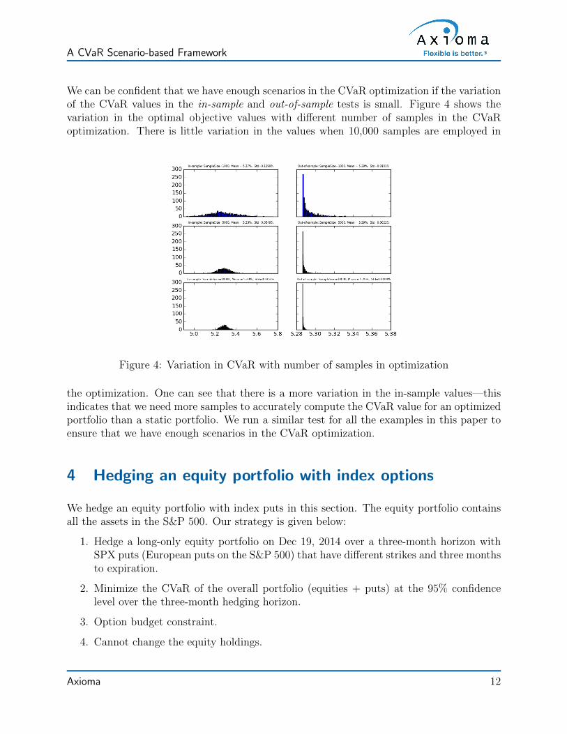
We can be confident that we have enough scenarios in the CVaR optimization if the variationof the CVaR values in the in-sample and out-of-sample tests is small. Figure 4 shows thevariation in the optimal objective values with different number of samples in the CVaRoptimization. There is little variation in the values when 10,000 samples are employed in

Figure 4: Variation in CVaR with number of samples in optimization

the optimization. One can see that there is a more variation in the in-sample values—thisindicates that we need more samples to accurately compute the CVaR value for an optimizedportfolio than a static portfolio. We run a similar test for all the examples in this paper toensure that we have enough scenarios in the CVaR optimization.

4 Hedging an equity portfolio with index options

We hedge an equity portfolio with index puts in this section. The equity portfolio containsall the assets in the S&P 500. Our strategy is given below:

1. Hedge a long-only equity portfolio on Dec 19, 2014 over a three-month horizon withSPX puts (European puts on the S&P 500) that have different strikes and three monthsto expiration.

2. Minimize the CVaR of the overall portfolio (equities + puts) at the 95% confidencelevel over the three-month hedging horizon.

3. Option budget constraint.

4. Cannot change the equity holdings.

Axioma 12

DRAFT


5. Only purchase puts.

It is worth emphasizing that one can also give the CVaR approach the flexibility to write puts.This can be done to collect the premium from suitable out-of-money puts and presumablysupplement the available budget, but we do not pursue put writing in this section. Thissection is organized as follows: We describe the CVaR approach for this example in Section4.1. Two parametric MVO approaches that use a linear model for the options are describedin Sections 4.2 and 4.3. We compare the CVaR approach with the MVO approaches inSection 4.4.

4.1 CVaR hedging

We first describe how we generate asset returns from the Monte Carlo simulation of riskfactors.

1. Step 1 of Algorithm 1 first generates the joint distribution(fE, f r, fσ

)∈ N (0,Σ) (9)

of the fundamental equity factor, risk-free rate, and implied volatility returns thatis assumed to follow a multivariate normal distribution N(0,Σ) with mean zero andcovariance Σ.

(a) Risk-free rate (LIBOR) returns f r include the one- and six-month factors. Weuse these factors to interpolate the three-month risk-free rate return that is usedto price the puts.

(b) Implied volatility returns fσ from the SPX volatility surface include the six-monthout-of-the-money, at-the-money, and in-the-money factors. We use the at-the-money factor to price the at-the-money puts, the out-of-the-money factor to pricethe out-of-the-money puts, and the in-the-money factor to price the in-the-moneyputs.

The asset-specific risk returns are then simulated from a multivariate normal distribu-tion with a diagonal covariance matrix Θ2. The fundamental equity factor, risk-freerate, implied volatility, and the asset-specific returns represent our choice of risk factorsfor the Monte Carlo framework. Note that the asset-specific returns are uncorrelatedwith the other risk factors and also with each other.

2. Equity returns come from the Axioma equity fundamental factor model as

rE = BfE + ε (10)

where B contains the equity exposures to the fundamental factors, fE contains thefundamental factor returns, and ε ∈ N (0,Θ2) contains the asset-specific returns whereΘ2 is a diagonal matrix containing the specific variances.

Axioma 13

DRAFT


3. The SPX put returns are generated from the Black-Scholes pricing model:

rO = BS (ru, f r, fσ) (11)

where ru = cT rE denotes the S&P 500 returns with c containing the S&P 500 weightson the rebalancing date. We illustrate the return computation for the ith SPX put inthe jth scenario below. Let S and r denote the current level of the S&P 500 and therisk-free rate, respectively.

(a) Let pi, Ki, σi, and Ti denote the current price, strike, implied volatility, and thetime to expiration of the ith option, respectively.

(b) Let ∆T denote the length of the hedging time horizon.

(c) Let Sj = S (1 + ruj), rj = (r + f r,j), and σji = σi (1 + fσ,j) denote the level of theS&P 500, risk-free rate, and the implied volatility in scenario j at the end of therebalancing time horizon.

(d) The Black-Scholes formula gives the price of ith SPX put in the jth scenario atthe end of the rebalancing time horizon as

pji = e−rj(Ti−∆T ) (KiΦ (−d2)− SjΦ (−d1)) (12)

where

d1 =log(Sj

Ki

)+(rj + 1

2

(σji)2)

(Ti −∆T )

σji√Ti −∆T

d2 = d1 − σji√Ti −∆T

and Φ() is the cumulative normal distribution function. The return of the ith putin the jth scenario is then given by

rO,ji =

(pji − pipi

).

4.2 MVO delta-rho-vega hedging

Consider the following delta-rho-vega linear model (see Hull [5]):

rOi = ∆i

(Supi

)ru +

(ρipi

)f r + νi

(σipi

)fσ (13)

for the ith option return, where pi, ∆i, ρi, σi, and νi represent the option share price, delta,rho, implied volatility, and vega, respectively; and Su represents the current level of the S&P500.

Axioma 14

DRAFT


Assuming that the equity returns rE are given by the linear factor model in equation (10),one can construct a linear model

rp = Gfp +Hε (14)

where rp =

(rE

rO

)denotes the asset returns; fp =

fE

f r

fσ

denotes the set of fundamental,

risk-free rate, and volatility surface factors; ε denotes the asset-specific risk factors; andG andH are matrices of appropriate dimensions. We assume that fp ∈ N (0,Σ), and ε ∈ N (0,∆2).It follows from equation (14) that the asset returns follow a multivariate normal distributionwhose covariance matrix is given by

Q =(GΣGT +HΘ2HT

).

Given portfolio holdings wp =

(wE

wO

), the risk of the portfolio is given by

Portfolio risk = (wp)T Qwp

= (wp)T(GΣGT +HΘ2HT

)wp.

(15)

The MVO delta-rho-vega approach minimizes the total risk of the portfolio subject to allthe constraints in the hedging strategy. A few comments are in order:

• The MVO delta-rho-vega approach is linearizing the options in the portfolio. Over theshort hedging horizon of three months, the option delta dominates the rho and thevega. In this setting, the MVO approach mimics the delta hedging approach commonlyused by traders.

• The MVO delta-rho-vega approach disregards the higher option moments, such as thegamma, that are important for longer hedging horizons.

• Since we are hedging the long-only equity portfolio with several index puts, the MVOdelta-rho-vega approach has multiple solutions since there are several ways to choosethe holdings in the SPX puts to effectively make the portfolio delta-neutral. In Section4.3, we show how one can incorporate some of the higher options moments in the hedgeby choosing an optimal portfolio that minimizes the portfolio gamma.

4.3 Enhanced MVO delta-gamma hedging

The MVO delta-gamma approach tries to incorporate option gamma in the MVO delta-rho-vega based hedging approach. Given that the MVO delta-rho-vega model has multiplesolutions, the MVO delta-gamma hedging chooses an MVO delta-rho-vega solution thatminimizes the portfolio gamma.

Axioma 15

DRAFT


The portfolio gamma is given by

Portfolio gamma =∑i∈O

(Γipi

)wi (16)

where O is the set of options in the portfolio, and Γi, pi, and wi denote the gamma, shareprice, and the dollar holding in the ith option, respectively. Note that only the options inthe portfolio contribute to the portfolio gamma.

The MVO delta-gamma follows a two level hierarchical process to generate the option hold-ings:

1. In level 1, we follow the MVO delta-rho-vega approach, where we minimize the portfoliorisk given by equation (15) subject to all the constraints in the hedging strategy.

2. In level 2, we minimize the portfolio gamma given by equation (16) subject to all theconstraints in Level 1 and an additional constraint prescribing that

Portfolio risk = (wp)T(GΣGT +HΘ2HT

)wp

≤ optimal objective value from Level 1 plus tolerance.

The solution to the Level 2 problem gives the option hedges.

4.4 Comparing the CVaR and MVO hedges

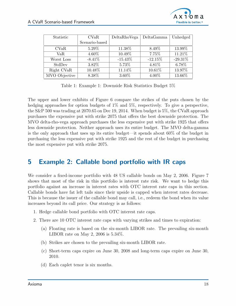
We compare the CVaR, MVO delta-rho-vega, and MVO delta-gamma optimized portfoliosfor different option budgets. The upper and lower exhibits in Figure 5 plot the histogram of50,000 realizations of the CVaR, delta-rho-vega, delta-gamma, and the unhedged portfolioreturns (in that order) at the end of the three-month rebalancing horizon, when the optionbudget is 1% and 5% of the reference size of the equity portfolio, respectively. The downsiderisk statistics for the different portfolios for a 5% budget are summarized in Table 1. Whenthe budget is small, the three hedges give similar results. However, when the budget is large,Table 1 shows that the CVaR portfolio return has the best downside risk statistics: The worstloss, CVaR, VaR, and standard deviation are much smaller than those of the MVO delta-rho-vega and MVO delta-gamma portfolios, respectively. Moreover, the right CVaR for theCVaR portfolio is only slightly smaller than that of the two MVO portfolios and the unhedgedportfolio showing that the CVaR portfolio has the best skew among these portfolios, i.e.,better downside without taking much away from the upside. Although the MVO delta-rho-vega objective values for the MVO delta-rho-vega and MVO delta-gamma portfolios aresmaller than the corresponding value for the CVaR hedged portfolio (not surprisingly, sincethese portfolios minimize this objective function), the downside risk statistics are worse. Thepoor performance of the MVO approaches can be attributed to the linear model for the putsthat does not capture the asymmetric payoffs of these instruments.

Axioma 16

DRAFT


(a) Budget 1%

(b) Budget 5%

Figure 5: Example 1: Histogram of future portfolio returns

Axioma 17

DRAFT


Statistic CVaR DeltaRhoVega DeltaGamma UnhedgedScenario-based

CVaR 5.29% 11.38% 8.49% 13.99%

VaR 4.60% 10.49% 7.75% 11.21%

Worst Loss -8.41% -15.43% -12.15% -29.31%

StdDev 3.82% 5.73% 4.81% 6.78%

Right CVaR 10.48% 11.14% 10.61% 13.97%

MVO Objective 8.38% 3.60% 4.00% 13.66%

Table 1: Example 1: Downside Risk Statistics Budget 5%

The upper and lower exhibits of Figure 6 compare the strikes of the puts chosen by thehedging approaches for option budgets of 1% and 5%, respectively. To give a perspective,the S&P 500 was trading at 2070.65 on Dec 19, 2014. When budget is 5%, the CVaR approachpurchases the expensive put with strike 2075 that offers the best downside protection. TheMVO delta-rho-vega approach purchases the less expensive put with strike 1925 that offersless downside protection. Neither approach uses its entire budget. The MVO delta-gammais the only approach that uses up its entire budget—it spends about 60% of the budget inpurchasing the less expensive put with strike 1925 and the rest of the budget in purchasingthe most expensive put with strike 2075.

5 Example 2: Callable bond portfolio with IR caps

We consider a fixed-income portfolio with 48 US callable bonds on May 2, 2006. Figure 7shows that most of the risk in this portfolio is interest rate risk. We want to hedge thisportfolio against an increase in interest rates with OTC interest rate caps in this section.Callable bonds have fat left tails since their upside is capped when interest rates decrease.This is because the issuer of the callable bond may call, i.e., redeem the bond when its valueincreases beyond its call price. Our strategy is as follows:

1. Hedge callable bond portfolio with OTC interest rate caps.

2. There are 10 OTC interest rate caps with varying strikes and times to expiration:

(a) Floating rate is based on the six-month LIBOR rate. The prevailing six-monthLIBOR rate on May 2, 2006 is 5.34%.

(b) Strikes are chosen to the prevailing six-month LIBOR rate.

(c) Short-term caps expire on June 30, 2008 and long-term caps expire on June 30,2010.

(d) Each caplet tenor is six months.

Axioma 18

DRAFT


(a) Budget 1%

(b) Budget 5%

Figure 6: Example 1: Overlays purchased by portfolios

Axioma 19

DRAFT


Figure 7: Sources of risk in callable bonds portfolio

3. Cannot change the callable bond holdings.

4. Experiment with budgets of 1% and 5% of the total market value of the callable bondportfolio.

5. Compare the CVaR and MVO hedges over a six-month hedging horizon.

We briefly describe the Monte Carlo pricer used to generate the asset scenarios below:

1. The Hull-White pricer (see Hull [5]) is used to price the callable bonds where thepricing factors include the US sovereign, swap, issuer credit, and swaption volatilityfactors.

2. Black’s formula (see Hull [5]) is used to price the caps as a sequence of caplets wherethe pricing factors include the US sovereign, swap, issuer credit, and the cap volatilitysurface factors.

The MVO approach linearizes both the callable bonds (the underlying instruments) and theIR caps (hedging overlays) to arrive at a covariance matrix for the portfolio.

The upper and lower exhibits in Figure 8 plot the histogram of 20,000 realizations of theCVaR and the MVO hedged portfolio returns at the end of the six-month hedging horizon,when the option budget is 1% and 5% of the reference size of the callable bond portfolio,respectively. The histogram of the unhedged callable bond portfolio returns for these realiza-tions is shown at the bottom of these two exhibits for comparison. Notice that the unhedgedcallable bond portfolio has a fat left tail since the upside of this portfolio is capped whenthe bonds are redeemed by the issuer. Table 2 presents the downside risk statistics for thedifferent portfolios. Notice that the CVaR portfolio has superior downside risk statistics

Axioma 20

DRAFT


(a) Budget 1%

(b) Budget 5%

Figure 8: Example 2: Histogram of future portfolio returns

Axioma 21

DRAFT


even for the small 1% budget: The worst-case return, left CVaR, left VaR, and standarddeviation are much smaller than that of the MVO portfolio. The MVO approach also doesnot use up its entire 1% budget and so the results are unchanged when one increases thebudget to 5%. On the other hand, the downside risk statistics for the CVaR portfolio onlyget better with the increased 5% budget.

Statistic CVaR 1% CVaR 5% MVO UnhedgedScenario-based Scenario-based

CVaR 3.58% 2.45% 4.41% 5.08%

VaR 2.86% 1.93% 3.49% 3.85%

Worst Loss -7.30% -4.92% -8.10% -9.13%

StdDev 1.71% 1.18% 1.99% 2.25%

Right CVaR 3.48% 2.40% 3.85% 4.27%

Table 2: Example 2: Downside risk statistics

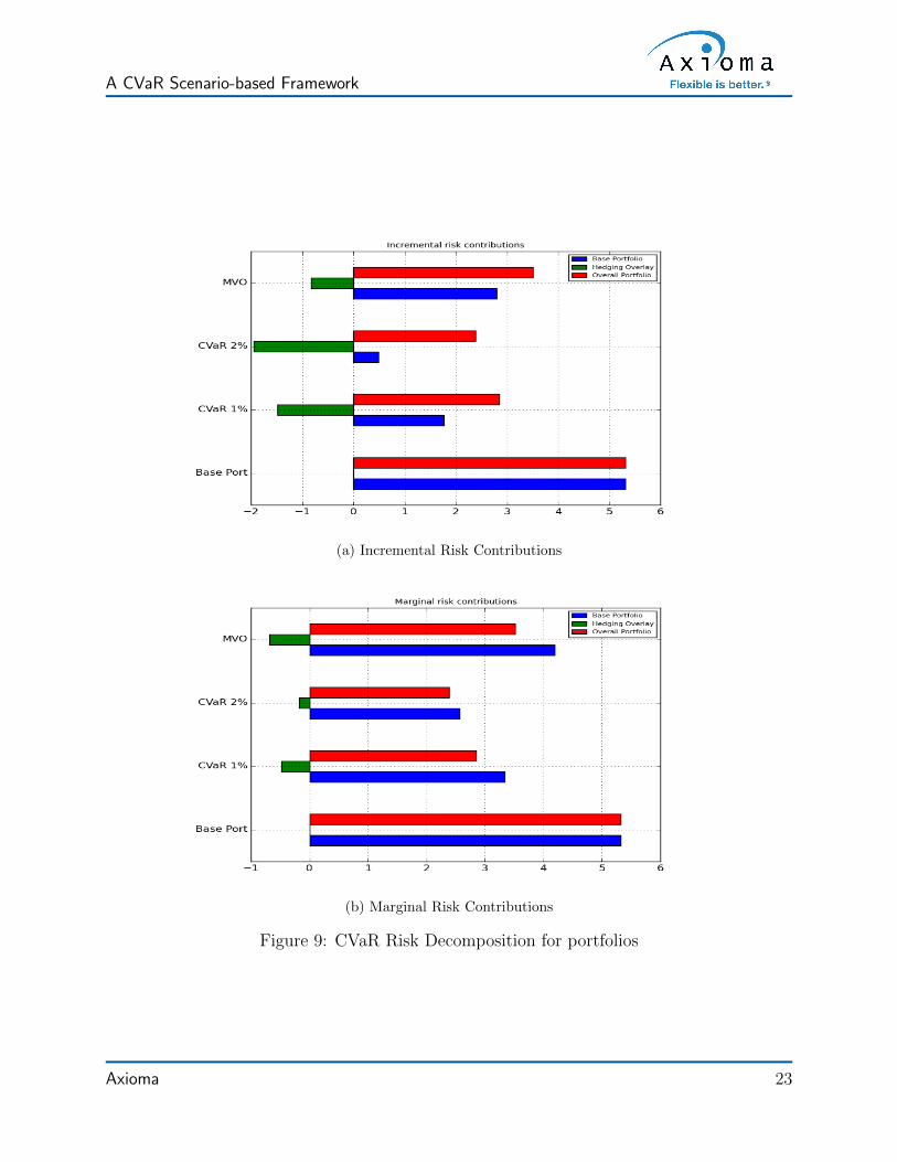
The upper exhibit of Figure 9 plots the incremental CVaR decompositions for the differentcomponents of the CVaR portfolios with 1% and 2% budgets and the MVO portfolio. Theincremental contribution for the overlays is the difference between the portfolio CVaR andthe CVaR of the base portfolio, i.e., the portfolio with the overlays removed. The incrementalcontributions for the overlays are negative for the three portfolios indicating that the overlaysare reducing the CVaR of the overall portfolio. Note that the greatest reduction in risk is forthe CVaR hedge with 2% budget. We used 10,000 scenarios to compute these contributions.The lower exhibit in Figure 9 plots the marginal CVaR decompositions for the differentcomponents of the three portfolios. The marginal CVaR of the overlay is the change inthe portfolio CVaR resulting from marginal changes in the overlay positions. Note that themarginal contribution for the overlay for the CVaR hedge with 2% budget is the smallestindicating that the portfolio CVaR is relatively insensitive, i.e., changes only slightly forsmall changes in the overlay positions. This is not surprising since this portfolio has thesmallest CVaR among the three portfolios.

The upper exhibit of Figure 10 plots the P/Ls for the CVaR, MVO, and unhedged portfolioswhen the portfolios are subject to instantaneous interest rate shocks ranging from -1% to 1%.An interest rate shock of 1% implies that we move the entire yield curve up by 1%. When ashock of 1% is applied, the base portfolio loses 6%, the MVO portfolio loses 4%, the CVaRportfolio with 1% budget loses 2%, and the CVaR portfolio with 5% budget loses nothing.On the other hand, when the entire yield curve moves down by 1%, the base portfolio gains5%, the MVO and the CVaR portfolios with 1% budget gain 4%, and the CVaR portfoliowith 5% budget gains 2%. Notice that the CVaR portfolio with 1% budget has a smallerdownside than the MVO portfolio while these portfolios have the same upside.

Axioma 22

DRAFT


(a) Incremental Risk Contributions

(b) Marginal Risk Contributions

Figure 9: CVaR Risk Decomposition for portfolios

Axioma 23

DRAFT


(a) Interest Rate Stress Tests

(b) Vega Stress Tests

Figure 10: Instantaneous Stress Tests

Axioma 24

DRAFT


6 Example 3: Convertible bond portfolio

In this example, we highlight the importance of utilizing appropriate pricing models thatcapture the key risks for a given strategy. We consider a portfolio which is comprised ofstocks and convertible bonds. For this portfolio, we compare two different pricing modelsfor convertible bonds where one model captures credit spread risk, whereas the other doesnot.

Before specifying the details of the portfolio (and overlays), we briefly comment about themodeling of convertible bonds. A convertible bond is a hybrid instrument that containsboth bond and equity-like features. An investor has the option to convert the bond into anumber of predefined shares, specified by the conversion ratio. The conversion feature givesconvertible bonds an embedded call option that increases when the underlying equity grows.For example, consider a convertible bond with a notional of e 1000 and a conversion ratio of25. If the underlying equity price rises to e 50, then the likelihood of conversion is high sinceits intrinsic call value is significantly greater than its notional (25×50 = 1,250 > 1,000).

In addition to the embedded call option, converts can contain other sources of optionalitysuch as call/put schedules, contingent conversion thresholds and soft call provisions.1 Figure11 presents two different equity profiles for a convertible bond. The dotted line represents theparity price of the convertible; for large stock prices, we expect the investor to convert intounderlying shares. The red line represents the typical payoff, which shows the asymmetricreturns from the embedded call option, namely, a large positive stock return will increase thevalue of a convert significantly, whereas a large negative stock return will have little impacton its return. Here, the investor still enjoys the bond component even though the upside fromthe equity component has been dampened. However, this scenario of floored protection fromnegative stock returns is unrealistic. As the stock value decreases significantly, we expectthe creditworthiness of the issuer to deteriorate. The solid blue line in Figure 11 depicts thiscase.

From a modeling perspective, there are various ways of collapsing the bond floor as the issuingfirm’s credit deteriorates. For example, Andersen and Buffum [1] introduce a jump-diffusionmodel and list common parameterizations of the intensity process that are monotonicallydecreasing functions of the stock price. Thus, as the stock price drops, the default intensityincreases, which in turn results in the collapse of the bond floor. In addition to defaultintensity or hazard rate models, structural (risk-neutral) models will also provide a linkfrom equity to credit. As the equity value deteriorates, the (risk-neutral) probability ofdefault increase since the value of the firm’s assets have decreased. In either modelingchoice listed above, a more realistic equity profile is the solid blue line in Figure 11. Forthis section, we will model the credit risk of the convertible bonds utilizing a risk-neutral

1Soft calls allow the issuer to redeem the bond at par only when the stock price is above a certainthreshold (this feature benefits the investor). Under contingent conversion conditions, investors can convertto underlying shares only when the stock price is above a specified threshold (this feature benefits the issuer).

Axioma 25

DRAFT


structural model.2

Now we turn to the composition of the base portfolio and the hedging overlays:

• The base portfolio under consideration is comprised of stocks and convertible bonds.The stocks are constituents of the Euro Stoxx 50, Stoxx Oil & Gas, PSI. The portfoliois long convertible bonds with short positions in the underlying stock; the convertiblebonds are in the energy sector.

• The overlay consists of an iTraxx Euro credit default index and a single name put thatreferences a convert for a Portuguese issuer.

The credit index is used to mitigate risk in the equity portfolio. Our intuition is that thecredit index is negatively correlated to the long equity positions, and, as a result, shouldhave a negative risk contribution when added to the base portfolio. However, there are alsoshort equity positions in the portfolio (from delta-hedging the convertible bonds), so it isunclear how much of the credit index might be selected. On the other hand, it is fairly clearthat the single name put should be selected. Intuitively, as we minimize CVaR, we expectthat the optimizer will select the put option since losses in the convertible bond will be offsetby gains in the put position.

Figure 11: Convertible bond payoff

We will compare the overlays chosen by the CVaR approach when we use: (a) Merton model

2In fact, we combine the structural model with a traditional equity lattice pricer.

Axioma 26

DRAFT


(blue line in Figure 11), and (b) simple pricing model (red line in Figure 11) that simplyprices the convertible bond as a bond with an embedded equity option without any creditspread risk. The left exhibit of Figure 12 shows the histogram of the different portfoliosat the end of the one-month hedging horizon. The right exhibit of Figure 12 shows theoverlays purchased by the CVaR portfolios with the simple and Merton convertible pricersfor a hedging budget of 1%. Note that the CVaR portfolio with the simple pricing modeldoes not purchase any overlays while the CVaR portfolio with the Merton pricing model usesabout 70% of its budget to purchase put protection. This is not surprising since only theMerton pricing model captures the credit spread risk of the convertible bond. The CVaRoptimization engine in Phase 2 of the hedging approach is only as good as the input scenariosand care should be taken to choose appropriate pricing models that capture the length ofhedging horizons, instruments characteristics, and the prevailing market conditions.

(a) Example 3: Histogram of future portfolio re-turns

(b) Example 3: Overlays purchased

Figure 12: Example 3: Compare portfolios

7 Conclusions

We presented a two-phase scenario-based CVaR hedging approach for minimizing the down-side risk in MAC portfolios. The base portfolio is fixed and the hedging approach determinesthe overlay holdings by minimizing the CVaR of the overall portfolio. The first phase of thehedging approach uses a Monte Carlo framework for generating the scenarios for the dif-ferent instruments in the portfolio. The second phase incorporates these scenarios in a

Axioma 27

DRAFT


scenario-based convex optimization problem to generate the overlay holdings. We comparethe CVaR approach with MVO-based approaches that linearize all the instruments in theportfolio on three examples and show that (a) the CVaR portfolio has better downside riskstatistics, and (b) the CVaR portfolio returns more attractive risk decompositions and stresstest numbers—tools that are commonly used by risk managers to evaluate the quality ofhedges.

We must emphasize that the CVaR hedging approach is flexible; this includes (a) choice ofthe risk factors and the pricing models in the Monte Carlo framework, and (b) the setupof the scenario-based convex optimization, including how it is regularized to return stableoptimal solutions. Ultimately, the CVaR hedging approach is not a standalone analysis andthe flexibility should be used wisely and in conjunction with other tools (risk decomposition,delta-hedging, stress testing) in the arsenal of the risk manager.

Axioma 28

DRAFT


References

[1] L. Andersen and D.B. Buffum (2003). Calibration and Implementation of Convert-ible Bond Models, Journal of Computational Finance, 7, 1–34.

[2] P. Artzner, F. Delbaen, J.M. Eber, and D. Heath (1999). Coherent Measuresof Risk, Mathematical Finance, 9(3), 203–228.

[3] P. Glasserman (2003). Monte Carlo Methods in Financial Engineering, Springer.

[4] J. Gotoh, K. Shinozaki, and A. Takeda (2013). Robust Portfolio Techniques forMitigating the Fragility of CVaR Minimization and Generalization to Coherent RiskMeasures, Quantitative Finance, 13, 1621–1635.

[5] J.C. Hull (2008). Options, Futures, and Other Derivatives, 7th edition, Prentice Hall.

[6] E. Jondeau and M. Rockinger (2006). Optimal Portfolio Allocation under HigherMoments, European Financial Management, 12(1), 29–55.

[7] G. Iyengar and A.K.C. Ma (2013). Fast Gradient Descent Rule for Mean-CVaROptimization, Annals of Operations Research, 205, 203–212.

[8] A. Kunzi-Bay and J. Mayer (2006). Computational Aspects of Minimizing Condi-tional Value-at-Risk, Computational Management Science, 3, 3–27.

[9] A. Lim, J.G. Shanthikumar, and G.Y. Yan (2011). Conditional Value-at-Risk inPortfolio Optimization: Coherent but Fragile, Operations Research Letters, 39, 163–171.

[10] H. Markowitz (1959). Portfolio Selection: Efficient Diversification of Instruments,Wiley.

[11] A.J. McNeil, R. Frey, and P. Embrechts (2015). Quantitative Risk Management:Concepts, Techniques, and Tools, Revised Edition, Princeton University Press.

[12] R.T. Rockafellar and S. Uryasev (2000). Optimization of Conditional Value-at-Risk, Journal of Risk, 2, 493–517.

[13] R.T. Rockafellar and S. Uryasev (2002). Conditional Value-at-Risk for GeneralLoss Distributions, Journal of Banking & Finance, 26, 1443–1471.

Axioma 29

DRAFT


A Robust CVaR formulation

Consider the robust CVaR problem

minw∈C

maxri∈Zi,i=1,...,s

CVaR(w, ε) (17)

where

Z i = {ri : ||Q−1/2(ri − ri)|| ≤ κ}. (18)

Let α be the VaR estimate variable. Define the auxiliary scenario variables

ui ≥ maxri∈Zi

max{(−ri)Tw − α, 0}, i = 1, . . . , s. (19)

The constraints that define these scenario variables can also be written as

minri∈Zi

(ri)Tw + α + ui ≥ 0,

ui ≥ 0, i = 1, . . . , s.

Using the alternative definition of the auxiliary scenario variables, we rewrite (17) as

minw,α,u

α +1

s(1− ε)

s∑i=1

ui

s.t. minri∈Zi

(ri)Tw + α + ui ≥ 0,

ui ≥ 0, i = 1, . . . , s,w ∈ C.

(20)

Minimizing a linear function over the ellipsoidal uncertainty set (18) can be done in closedform. We have

minri∈Zi

(ri)Tw = (ri)Tw − κ√wTQw, i = 1, . . . , s. (21)

Plugging in the scenario equations (21) into the model (20) and introducing a new vari-able

α =(α− κ

√wTQw

)helps us write the model (20) as

minw,α,u

α +1

s(1− ε)

s∑i=1

ui + κ√wTQw

s.t. (ri)Tw + α + ui ≥ 0,ui ≥ 0, i = 1, . . . , s,w ∈ C.

(22)

This shows that the robust CVaR problem has an additional risk term in the objectivefunction and is a scenario-based, second-order cone program.

Axioma 30

United States and Canada: 212-991-4500

Europe: +44 20 7856 2451

Asia: +852-8203-2790

New York OfficeAxioma, Inc.17 State StreetSuite 2700New York, NY 10004

Phone: 212-991-4500Fax: 212-991-4539

London OfficeAxioma, (UK) Ltd.30 Crown PlaceLondon, EC2A 4E8

Phone: +44 (0) 20 7856 2451Fax: +44 (0) 20 3006 8747

Geneva OfficeAxioma CHRue du Rhone 69, 2nd Floor1207 Geneva, Switzerland

Phone: +41 22 700 83 00

Atlanta OfficeAxioma, Inc.400 Northridge RoadSuite 850Atlanta, GA 30350

Phone: 678-672-5400Fax: 678-672-5401

Hong Kong OfficeAxioma, (HK) Ltd.Unit B, 17/F30 Queen’s Road CentralHong Kong

Phone: +852-8203-2790Fax: +852-8203-2774

San Francisco OfficeAxioma, Inc.201 Mission StreetSuite #2150San Francisco, CA 94105

Phone: 415-614-4170Fax: 415-614-4169

Singapore OfficeAxioma, (Asia) Pte Ltd.30 Raffles Place#23-00 Chevron HouseSingapore 048622

Phone: +65 6233 6835Fax: +65 6233 6891

Sales: [email protected]

Client Support: [email protected]

Careers: [email protected]

DRAFT

draft - optimization · pdf filedraft a cvar scenario ... portfolio construction is...

Documents