draft drecp and eir/eis – appendix f1, methods for megawatt · pdf file ·...
TRANSCRIPT

Appendix F
Megawatt Distribution

Appendix F1
Methods for Megawatt Distribution

Draft DRECP and EIR/EIS APPENDIX F1. METHODS FOR MEGAWATT DISTRIBUTION
Appendix F1 F1-1 August 2014
F1 METHODS FOR MEGAWATT DISTRIBUTION
F1.1 Introduction
This appendix describes the method used to estimate the distribution of generation from
which impacts to Covered Activities were derived. This appendix is divided into five sections:
The overview describes the overarching approach used to estimate the distribution
of impacts and the strategy used to overcome uncertainty in the future distribution
of generation.
The Development Focus Area (DFA) distribution section primarily discusses the
effects of policies enacted by regional stakeholders, focusing primarily on polices
that may lead to exclusion of generation development.
The distribution of impacts within DFAs section discusses, in detail, the method
used to capture factors that influence the distribution of generation between
different subareas and different jurisdictions within DFAs.
The summary of distribution input scenarios provides a narrative description of each
scenario that was used to construct the generation distribution for each alternative.
The method for distribution section provides a description of the mechanics by
which different factors were combined for each scenario, and a description of the
input scenarios were combined into a single aggregated scenario.
F1.2 Overview
Estimating the likely distribution of renewable energy development within the Desert
Renewable Energy Conservation Plan (DRECP) has the overarching objective of ensuring
that the plan evaluates a plausible magnitude of effects for each covered biological
resource such that the plan offers adequate coverage for activities related to renewable
energy development.
There is inherent uncertainty in estimating the future distribution of generation impacts.
Many factors may ultimately affect what and where technology may be developed; and the
interplay of these factors is unknown. Further, it is likely that generation development
could aggregate in specific regions, and as a consequence impacts may be higher in some
areas with corresponding lower impacts in other areas. Accurately predicting this
aggregation is not possible and cannot be identified with any precision.
Any method developed to estimate the likely impacts needs to account for uncertainty in
both the underlying factors influencing development and the possibility of aggregation of
development. No single scenario can feasibly represent the variability that arises from such
uncertainty because different equally plausible scenarios may be contradictory in their

Draft DRECP and EIR/EIS APPENDIX F1. METHODS FOR MEGAWATT DISTRIBUTION
Appendix F1 F1-2 August 2014
outcomes. For example, a scenario that expresses aggregation of development on private
lands would result in low impacts to public lands and vice versa. Each scenario would
inadequately describe an alternative, equally plausible outcome.
To overcome the limitations of a single scenario, the following method describes a process
by which several scenarios that each represent different development trajectories were
combined. This method builds in the flexibility necessary for the DRECP to operate
successfully under many possible futures.
Each scenario represented a plausible narrative based on different combinations of
factors developed from agency and stakeholder input. It should be noted that this form
of scenario planning is not intended to be probabilistic or representative of the most
likely future conditions. It is rather meant to account for a set of alternative futures
(Mohamoud et al. 2009).
Several factors were identified that affect the ultimate distribution of generation. Factors
may be associated with the technology (e.g., acreage per megawatt [MW]), or they may be
technology independent and associated with a particular region of the Plan Area. Each
scenario was built up from a unique combination of factors, and the scenarios were in turn
combined into a final distribution of generation. Exhibit F1-1 illustrates the relationship
between the different factors, the scenarios, and the ultimate distribution of Covered
Activities analyzed in each alternative. All scenarios were developed with a defined
development goal of achieving 20,323 MWs of generation within the DFAs in the Plan Area
over the lifetime of the DRECP.
The ultimate distribution of Covered Activities used for the alternatives impacts
analysis was built from elements within all scenarios. The following method used a
bottom-up approach and combined the maximum likely generation values for any given
set of DFAs from a variety of elements across all scenarios. For example, the subarea
maximum for wind generation may be in scenario 1, whereas the maximum for solar
may occur in scenario 3. By combining elements in this way, it was possible to develop
an impact scenario that represented locally high impacts but was set within a plausible
framework of assumptions.
As a consequence of this approach, the combined output scenario for each alternative
summed to greater than 20,323 MWs of generation. This was purely an artifact of
providing planning flexibility, and 20,323 MW would still be considered as a cap on
future development coverage.

Draft DRECP and EIR/EIS APPENDIX F1. METHODS FOR MEGAWATT DISTRIBUTION
Appendix F1 F1-3 August 2014
Exhibit F1-1 The Relationship between Factors Affecting Generation
Distribution, Scenarios, and the Aggregated Final Scenario used to Analyze the
Distribution of Covered Activities for Each Alternative
F1.3 DFA Distribution
The following section briefly discusses factors that affect the distribution of DFAs. The main
factor that affected the distribution of DFAs was the reserve design and existing legally and
legislatively protected areas. Since these aspects of the distribution of DFAs are extensively
covered in the main body of the document, the following discussion focuses on federal,
state, and local polices that may act to preclude generation from areas within the Plan Area.
F1.3.1 Reserve Design
The reserve design was the single most important factor affecting the likely distribution of
DFAs. An extensive description of the reserve design and factors affecting the reserve
design is provided in Section I.3.4.4 of the DRECP and not covered here.
F1.3.2 Development Restriction Factors
Regulatory policy and jurisdictional constraints may act to preclude generation from siting
in some areas of the DRECP. In particular, the restrictions placed on wind development by
Los Angeles County and Department of Defense (DOD), and the restrictions placed on some
types of solar technology by DOD, were considered important in influencing the future
distribution of generation.
DOD development restrictions on tall structures to the north and east of Edwards Air Force
Base preclude the development of wind turbines and certain solar technologies. Similarly,

Draft DRECP and EIR/EIS APPENDIX F1. METHODS FOR MEGAWATT DISTRIBUTION
Appendix F1 F1-4 August 2014
Los Angeles County actions have generally been to deny wind development within the Plan
Area. The effect of applying these restrictions for the life of the DRECP would considerably
reduce the area available for wind development. As a consequence, any future generation
profile would be more heavily weighted toward solar development. Analysis indicates that
in the absence of the described restrictions wind could make up 16% to 35% of the
possible generation profile; whereas with such restrictions in place, wind could make up
between 8.5% to 14% of a possible generation profile (see Box 1, which describes
estimated impacts on wind generation).
In assessing the likelihood of policy changes on the part of DOD, the Renewable Energy
Action Team (REAT) agencies concluded that the DOD policy would not be lifted for the
foreseeable future. Consequently it was assumed that, for the life of the DRECP, wind
development would be excluded from the areas described above. The effect of DOD height
restrictions on the distribution of solar generation was considered to be less critical, since
it only affects technologies that require tall structures, such as solar power towers. It was
the consensus of the REAT agencies that DOD restrictions would not affect the overall
potential for development of other solar generation because the areas would still be
available to solar photovoltaic (PV) and other solar technologies.
In assessing the likelihood of policy changes on the part of Los Angeles County, the REAT
agencies considered the permitting of wind development as a possibility over the lifetime
of the DRECP. Therefore, in certain alternatives, wind DFAs were identified in Los Angeles
County and generation distributed accordingly.

Draft DRECP and EIR/EIS APPENDIX F1. METHODS FOR MEGAWATT DISTRIBUTION
Appendix F1 F1-5 August 2014
Box 1
Estimated Impacts of Department of Defense and Los Angeles County
Restrictions on Potential Wind Generation Development
Analysis of generation distribution in the presence and absence of Los Angeles County and
DOD restrictions were undertaken on earlier, but similar, versions of the Preferred
Alternative. Exhibit B-1 describes the consequence of exclusionary policies on the likely
quantity of wind in the overall generation profile. Typical values for siting discount factors
range from 3 to 5 (see Section F1.4.3 for details), giving contrasting range of wind values of
between 7,193 and 2,375 MWs between no restrictions with low discount factors and all
restrictions with high discount factors. The result is a potential difference of 4,818 MW.
Exhibit B-1
Potential Range of Generation Capacity (MW) for Wind under Different
Restriction Criteria
-
2,000
4,000
6,000
8,000
10,000
12,000
2 4 6 8
MW
Siting Discount Factor
Wind Base Case
Wind No DODrestrictions
Wind No DODrestrictions,No LA Countyrestrictions

Draft DRECP and EIR/EIS APPENDIX F1. METHODS FOR MEGAWATT DISTRIBUTION
Appendix F1 F1-6 August 2014
F1.4 Distribution of Impacts within DFAs
The following section discusses the parameters affecting the generation distribution
between DFAs in different subareas and different jurisdictions. The following information
was common to all scenarios and sought to simultaneously account for the area available to
each technology, potential interactions between technologies, and variation in the relative
development potential of different DFAs.
For the purpose of estimating generation distribution across the DFAs, a simple conditional
model was developed. The DFAs were grouped by ecoregional subarea (e.g., West Mojave
and Eastern Riverside – 6), jurisdiction (e.g., Bureau of Land Management [BLM], California
State Lands Commission [CSLC], private, county), and compatible technologies (e.g., areas
that allowed both wind and solar were grouped, areas that were exclusively solar only
were grouped, etc.).
Generation was assumed to be distributed in direct proportion to the area available within
a given set of DFAs. However, on its own, this assumption is overly simplistic and takes
account of neither the requirements of different technologies nor the heterogeneity of
factors affecting development across the Plan Area. Therefore, the assumption was
modified by two factors: The first is the acreage yield factor, a quantity directly related to
the footprint of the technology (Table F1-1). The second factor is the siting discount factor,
which is related to the positive and negative influences acting upon development in a
particular group of DFAs. The relationship between these factors is summarized in
Equation 1 and discussed in more detail below.
Equation 1
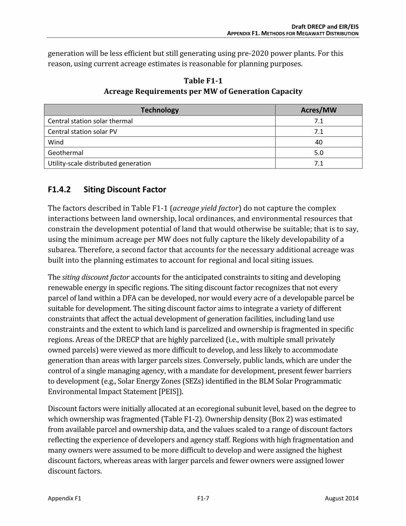
F1.4.1 Acreage Yield Factor
The acreage yield factor represents the minimum acreage requirement necessary to
generate 1 MW of energy. As is evident from Table F1-1, this requirement is different for
each technology. The estimates for each technology were derived from actual projects in
California, and they were based on the same information and analysis used to develop the
California Energy Commission (CEC) calculator.
It should be noted that for all scenarios, the acreage requirements associated with each
technology were held constant. Although technological changes may impact future yields per
acre, estimating these changes with any accuracy is not possible. Further, the incremental
introduction of technological improvements would lead to only a gradual reduction in the
average acreage requirements across the entire Plan Area. For example, the availability of a
much more efficient solar PV technology in 2040 could be expected to only have a small
effect on the plan-wide average yield because a significant component of the DRECP’s PV
Draft DRECP and EIR/EIS APPENDIX F1. METHODS FOR MEGAWATT DISTRIBUTION
Appendix F1 F1-7 August 2014
generation will be less efficient but still generating using pre-2020 power plants. For this
reason, using current acreage estimates is reasonable for planning purposes.
Table F1-1
Acreage Requirements per MW of Generation Capacity
Technology Acres/MW
Central station solar thermal 7.1
Central station solar PV 7.1
Wind 40
Geothermal 5.0
Utility-scale distributed generation 7.1
F1.4.2 Siting Discount Factor
The factors described in Table F1-1 (acreage yield factor) do not capture the complex
interactions between land ownership, local ordinances, and environmental resources that
constrain the development potential of land that would otherwise be suitable; that is to say,
using the minimum acreage per MW does not fully capture the likely developability of a
subarea. Therefore, a second factor that accounts for the necessary additional acreage was
built into the planning estimates to account for regional and local siting issues.
The siting discount factor accounts for the anticipated constraints to siting and developing
renewable energy in specific regions. The siting discount factor recognizes that not every
parcel of land within a DFA can be developed, nor would every acre of a developable parcel be
suitable for development. The siting discount factor aims to integrate a variety of different
constraints that affect the actual development of generation facilities, including land use
constraints and the extent to which land is parcelized and ownership is fragmented in specific
regions. Areas of the DRECP that are highly parcelized (i.e., with multiple small privately
owned parcels) were viewed as more difficult to develop, and less likely to accommodate
generation than areas with larger parcels sizes. Conversely, public lands, which are under the
control of a single managing agency, with a mandate for development, present fewer barriers
to development (e.g., Solar Energy Zones (SEZs) identified in the BLM Solar Programmatic
Environmental Impact Statement [PEIS]).
Discount factors were initially allocated at an ecoregional subunit level, based on the degree to
which ownership was fragmented (Table F1-2). Ownership density (Box 2) was estimated
from available parcel and ownership data, and the values scaled to a range of discount factors
reflecting the experience of developers and agency staff. Regions with high fragmentation and
many owners were assumed to be more difficult to develop and were assigned the highest
discount factors, whereas areas with larger parcels and fewer owners were assigned lower
discount factors.

Draft DRECP and EIR/EIS APPENDIX F1. METHODS FOR MEGAWATT DISTRIBUTION
Appendix F1 F1-8 August 2014
Table F1-2
Siting Discount Factors Used for Each Scenario
DRECP Subarea 3–5 Factor Range1 3–10 Factor Range2
Cadiz Valley and Chocolate Mountains (East Riverside) 3 3
Imperial Borrego Valley (Imperial Valley) 3 3 to 4
Kingston and Funeral Mountains 4 5
Mojave and Silurian Valley 4 3 to 5
Owens River Valley 3 3
Panamint Death Valley 3 3
Pinto Lucerne Valley and Eastern Slopes 3 to 4 3 to 6
Piute Valley and Sacramento Mountains 3 3
Providence and Bullion Mountains 3 3 to 5
West Mojave and Eastern Slopes (West Mojave) 3 to 5 3 to 10 1 Used in scenario 1. 2 Used in scenarios 2–5.
Box 2
Ownership Density Explanation
The average number of parcels and number of owners for each subarea were estimated
from existing mapped parcel and ownership data by California Department of Fish and
Wildlife (CDFW) biogeographical unit for both areas within DFAs and for the wider
subareas. The number of unique owners and parcels within each subarea was counted,
and the average was determined by dividing the count by the total acreage of the DFA or
subarea. Results were then scaled to owners per 1,000 acres to provide a meaningful
approximation of average density. As is evident from Table B-2 the average densities
within DFAs were generally higher than the average densities for the wider subarea.
Because density estimates could not be used in their raw form, they were ranked, binned,
and rescaled to provide the basis for the distribution of discount factors, with the highest
density equating to the highest discount factors.
Table B-2
Average Parcel and Ownership Density for Different Subareas within the DRECP
DRECP Subarea
Within DFA
All Subarea
Within DFA
Within Subarea
Parcels/1,000 acres Owner/1,000acres
Cadiz Valley and Chocolate Mountains – 1 No DFAs 10 No DFAs 2
Cadiz Valley and Chocolate Mountains – 2 25 13 7 4
Cadiz Valley and Chocolate Mountains – 3 No DFAs 8 No DFAs 3
Imperial Borrego Valley – 1 37 75 12 23

Draft DRECP and EIR/EIS APPENDIX F1. METHODS FOR MEGAWATT DISTRIBUTION
Appendix F1 F1-9 August 2014
Table B-2
Average Parcel and Ownership Density for Different Subareas within the DRECP
DRECP Subarea
Within DFA
All Subarea
Within DFA
Within Subarea
Parcels/1,000 acres Owner/1,000acres
Imperial Borrego Valley – 2 20 38 8 8
Imperial Borrego Valley – 3 6 5 Missing 1
Kingston and Funeral Mountains – 1 65 2 53 Missing
Mojave and Silurian Valley – 1 90 22 56 10
Mojave and Silurian Valley – 2 No DFAs 4 No DFAs 1
Owens River Valley – 1 47 12 3 3
Panamint Death Valley – 1 No DFAs 3 No DFAs Missing
Pinto Lucerne Valley and Eastern Slopes – 1 139 62 78 42
Pinto Lucerne Valley and Eastern Slopes – 2 204 47 0 33
Piute Valley and Sacramento Mountains – 1 No DFAs 8 No DFAs 2
Providence and Bullion Mountains – 1 65 6 35 2
Providence and Bullion Mountains – 2 15 8 Missing 2
West Mojave and Eastern Slopes – 1 208 43 89 14
West Mojave and Eastern Slopes – 2 126 119 81 60
West Mojave and Eastern Slopes – 3 No DFAs 38 No DFAs 26
West Mojave and Eastern Slopes – 4 244 257 158 102
West Mojave and Eastern Slopes – 5 247 293 114 155
West Mojave and Eastern Slopes – 6 110 70 56 30
F1.4.3 Discount Factor Ranges
The range of discount factors used was critically important to the final distribution of
generation. A low range of discount factors effectively means there is little differential
selection between different DFAs, and that impacts are relatively evenly distributed across
the different DFAs. Conversely, a high range of discount factors means that DFAs are highly
differentiated (i.e., there is a high contrast between developability of different DFAs). This
results in low levels of development in areas with high discount factors, and the reverse in
areas with low discount factors. To assess the impact of different ranges, scenario 1 used a
smaller range of potential discount factors ranging from 3 to 5; whereas scenarios 2–5 used
discount factors ranging from 2 to 10.

Draft DRECP and EIR/EIS APPENDIX F1. METHODS FOR MEGAWATT DISTRIBUTION
Appendix F1 F1-10 August 2014
F1.4.4 Public vs. Private land
It is unknown the extent to which having a single owner/manager and implementing
policies such as the Solar PEIS on public land would reduce barriers to development. It was
possible to explore the likely impacts of such factors aimed at encouraging generation by
modifying the discount factors for areas managed by these lands managers. Conceptually, if
policies are successful, then CSLC- and BLM-managed land would be expected to draw a
disproportionately large portion of the eventual development. In contrast, if the polices
have no effect on developer preference, then public land would draw a proportionately
similar quantity of development to private land. The effect of implementing successful
polices were simulated in scenarios 3–5 (Exhibit F1-2). In these scenarios, the discount
factors for BLM and CSLC DFAs were reduced to two.
F1.4.5 Imperial Borrego Valley Considerations
As stated previously, the degree of ownership fragmentation was a starting point. Discount
factors were further modified based on stakeholder input. In particular, Imperial County
was identified as exhibiting a limited tolerance to development; both Imperial County and
Imperial Irrigation District (IID) expressed concerns over the likely extent of generation
that may be sited in the region. While not precluding generation, pressure from other land
uses such as agriculture may act to reduce the likelihood of development.
Further, the feasibility of constructing sufficient transmission to export energy may
limit development in Imperial DFAs. Evidence developed by DRECP and the
Transmission Technical Group (TTG) suggests that Imperial DFAs could be limited by
transmission constraints (Table F1-3). TTG report #1 (TTG et al. 2012) identified
transmission sufficient to deliver 11,109 MWs from Imperial (for the high 2050
scenario), while IID identified the July 2012 Briefing Book scenario with 15,702 MW of
generation in Imperial as infeasible due to transmission constraints (Dudek 2012). Both
scenarios identified considerably less generation than the 25,473 MWs theoretical ly
possible based on available acreage (Table F1-1). Even an 11,000 MW estimate may be
excessive if counties are unwilling to develop prime agricultural land. Known limits for
transmission (where available), in conjunction with a range of assumed agricultural
land impacts, provided a credible boundary for the maximum generation in Imperial.
These analyses are presented as a sequence of constraints in comparison to a
theoretical maximum based on acreage, similar to Table F1-3 and Exhibit F1-2.
In conclusion, such limited tolerance did not exclude development but simply reduced the
likelihood of development occurring in a particular area. The limitations to development
for Imperial were expressed by increasing the discount factors to 6 associated with this
region in scenario 5.

Draft DRECP and EIR/EIS APPENDIX F1. METHODS FOR MEGAWATT DISTRIBUTION
Appendix F1 F1-11 August 2014
-
5,000
10,000
15,000
20,000
25,000
30,000
Northern Mojave E Riverside Imperial
MW
Sub-regions within the DRECP Plan area
Theoretical maximumpossible based acreageavailable within DFA
Maximum exportcapacity based on TTGanalyzed scenarios
DFA acreage
Transmission Driven limits
Table F1-3
Comparison between the Maximum Theoretical Solar Generation Based on Acreage
and the Maximum Analyzed Export Capacity for Major Regions within the DRECP
Theoretical Maximum MW Possible Based on
Acreage Available within DFA1
Maximum Export MW Capacity Based
on TTG Analyzed Scenarios
Acreage and Transmission
Constrained Limit for Solar
Northern Mojave 20,109 27,2232 20,109
East Riverside 11,343 >2,7173 but < 4,1384 2,717–4,138
Imperial 25,473 >11,1092 but < 15,7024 11,109–15,702
Total Capacity 56,924 41,049 33,935–39,949 1 April 16, 2013, Preferred Alternative DFA configuration. 2 April 2012 TTG report (TTG et al. 2012) 2050 scenario analyzed limit. 3 December 2012 TTG report (TTG 2012) Alternative 5 analyzed limit. 4 July 10, 2012, Briefing Book (Dudek 2012), and assessed by TTG December 2012 (TTG 2012). Note: For this analysis, the northern Mojave includes west Mojave, Barstow, Interstate 15 corridor, and Owens Valley.
Exhibit F1-2 Factors Limiting Maximum Development within the Plan Area
Note: For this analysis, the northern Mojave includes west Mojave, Barstow, Interstate 15 corridor, and Owens Valley.

Draft DRECP and EIR/EIS APPENDIX F1. METHODS FOR MEGAWATT DISTRIBUTION
Appendix F1 F1-12 August 2014
F1.5 Summary of Input Scenarios
Five scenarios were developed that represented different combinations of factors and
assumed different strengths of interactions between different jurisdictions, ecoregional
subareas, and counties. In developing the set of scenarios, the degree to which ownership
was fragmented was used as the basis for assessing the likelihood of energy development
in each subarea. The effects of ownership fragmentation were then modified by modeling
weak or strong selective forces between area differences (scenario 1 vs. scenarios 2–5), by
modeling alternative outcomes of policies undertaken by BLM and CSLC (scenarios 1–2 vs.
scenarios 3–5), and in response to issues raised by stakeholders (scenario 5). Exhibit F1-3
illustrates the relationships and differences between the input scenarios.
The following section provides a narrative summary of each scenario, so as to better
conceptualize what it represents and how it fits with other scenarios. Scenarios 1 and 2
represent development trajectories within which impacts to private and public land were
neutral (i.e., there were no preferences made by developers in response to policies
implemented on public lands). Scenarios 3–5 represent development trajectories within
which publicly administered land was favored by developers. Finally, scenario 5 accounts
for potential restrictions to development associated with the Imperial Borrego Valley
subarea. A more detailed description of each scenario is presented below.
F1.5.1 Scenario 1
Scenario 1 assumed that there was relatively little difference in the positive and negative
influences acting on generation across the Plan Area, and that the policies of BLM and CSLC
had no effect on the distribution of renewable energy development. Consequently, this
scenario assumed no difference in selection of public vs. private lands. Discount factors
range from 3 (i.e., maximum of 33% of DFAs developed) to 5 (i.e., maximum of 20% of
DFAs developed). Distribution was based on the degree of ownership fragmentation, with
no modification for BLM- and CSLC-administered lands.
F1.5.2 Scenario 2
Scenario 2 assumes much greater differentiation as a consequence of ownership
fragmentation within the Plan Area. Regions such as the West Mojave exhibit high degrees
of ownership fragmentation and were assigned the highest discount factors based on
ownership density, measured as number of owners per 1,000 acres. Discount factors range
from 3 to 10 based on the degree of ownership fragmentation, with no modification for
BLM- and CSLC-administered lands.

Draft DRECP and EIR/EIS APPENDIX F1. METHODS FOR MEGAWATT DISTRIBUTION
Appendix F1 F1-13 August 2014
Exhibit F1-3 Illustrates the Relationship between Ownership Density,
Discount Factors, and Each Scenario Used to Construct Final Combined Scenario
Used for Impacts Analysis
F1.5.3 Scenario 3
Scenario 3 builds on the ownership fragmentation described in scenario 2 but further
assumes that policies undertaken by CSLC and BLM act as incentives to development and
ultimately result in more renewable energy development on lands administered by these
agencies. However, it also assumes that these outcomes would primarily influence
development in the West Mojave portion of the Plan Area. Discount factors range from 3 to
10 based on the degree of ownership fragmentation, with DFAs administered by BLM and
CSLC in the West Mojave assumed to have an adjusted discount factor as low as 2.
F1.5.4 Scenario 4
Scenario 4 builds on the ownership fragmentation described in scenario 2 but further
assumes that policies undertaken by CSLC and BLM act as incentives to development and
ultimately result in more renewable energy development on lands administered by these
agencies. Discount factors range from 3 to 10 based on the degree of ownership
fragmentation, with DFAs administered by BLM and CSLC across the Plan Area assumed to
have an adjusted discount factor as low as 2.

Draft DRECP and EIR/EIS APPENDIX F1. METHODS FOR MEGAWATT DISTRIBUTION
Appendix F1 F1-14 August 2014
F1.5.5 Scenario 5
Scenario 5 is identical to scenario 4 but assumes that the presence of high-quality farmland
in the Imperial Valley acts as a negative influence to development. Discount factors range
from 3 to 10 based on the degree of ownership fragmentation, with DFAs administered by
BLM and CSLC across the Plan Area assumed to have an adjusted discount factor as low as
2. Further, private land DFAs within the Imperial Borrego Valley subarea are assumed to
have a high discount factor of 6.
F1.6 Method for Distributing Generation between DFAs
The above section described the various parameters that were developed to model the
influence of different factors on the distribution of generation. The following section
describes the rules and mechanism by which generation capacity (MWs) was distributed
across the DFAs to enable the estimation of impacts from Covered Activities.
For the purpose of estimating generation distribution across the DFAs, a simple conditional
model was developed. The DFAs were grouped by ecoregional subarea, jurisdiction, and
compatible technologies.
The following four criteria were identified by the REAT and defined as the basis for
any distribution:
1. No more generation would be developed than is required to meet the target
generation requirements. The Plan Area would be expected to permit no more than
20,323 MWs of renewable energy generation (i.e., no more than that would be
evaluated for permitting within the framework of the DRECP).
2. Geothermal and ground-mounted distributed generation (i.e., generation of 20
MWs) were fully developed in all scenarios. Geothermal was maximized because it
can provide benefits similar to baseload generation. Distributed generation was
maximized to assist with meeting state energy policy goals for this technology.
Consequently, the only variability was between solar and wind generation.
3. DFAs were not exclusive to a single technology. That is to say there is overlap
between technologies, and thus areas of the DRECP within which technologies may
compete for space. Where there was competition between technologies, it was
assumed to be symmetrical (i.e., no judgment, bias in success, or preference was
given to competing wind and solar technologies).
4. Generation was distributed proportionately across the DFAs. The distribution is
directly proportional to the acreage available within a DFA. However, this may be
modified by factors that affect the overall developability as discussed above.

Draft DRECP and EIR/EIS APPENDIX F1. METHODS FOR MEGAWATT DISTRIBUTION
Appendix F1 F1-15 August 2014
In order to apply the above criteria, a series of more-detailed assumptions were necessary,
which are described in Table F1-4.
Table F1-4
Describing the Assumptions and Rules for Distributing
Generation across Development Focus Areas
Rule Explanation
All acreage within the DFAs or a particular DFA subarea was considered to be of equal value.
If a DFA was suitable for a particular technology, then the whole of that subarea was of equal value for that technology.
Each DFA accommodates the generation capacity that was proportional to the energy resource that it contains. The area (acreage) of a DFA was a direct measure of the amount of resources available.
All insolation and wind speed values within a DFA are assumed equal, and as a consequence area was a good proxy for the energy potential. The DRECP was effectively split into a binary state: areas suitable for development (DFAs) and unsuitable for development (not DFAs).
No two technologies can have overlapping acreage (i.e., technologies are fully mutually exclusive).
Although some hybrid generations systems may be developed, for simplicity, development was considered non-overlapping.
For the purposes of estimating the distribution of generation capacity (MWs) across the DFAs, each technology has a constant set of characteristics.
Energy yield per acre was technology dependent; consequently, the minimum acreage requirements to accommodate the expected generation was dependent upon the assumptions made about technology mix. The yield represents the minimum acreage required to generate a MW of energy. The specific assumptions made concerning the average acres per MW of generation capacity for each technology are as follows: 7.1 acres/MW solar, 40 acres/MW wind, 5 acres/MW geothermal.
Utility-scale distributed generation was considered technology neutral but defined as requiring 7.1 acres per MW. However, to account for small (1–5 MW) urban/suburban and infill projects, only 80% of all utility-scale distributed generation MWs are assumed to require development acreage.
For the purposes of estimating the distribution of generation capacity (MWs) across the DFAs, the DFA development barriers/complexity was represented by the discount factor that was a property of the DFA (i.e., not the technology).
The process of siting, permitting, and constructing a facility requires more land than the minimum acreage assumed necessary for energy generation. To account for the many factors that may affect the location and configuration of a project, a discount factor was developed. The discount factor was discussed in detail in the main body of this document.
Geothermal and utility-scale distributed generation are developed to their full capacity as assumed by CEC.
As a consequence, these technologies are assumed to be fully developed and are effectively a constant in all scenarios. They are not subject to the competitive effects of wind or solar.

Draft DRECP and EIR/EIS APPENDIX F1. METHODS FOR MEGAWATT DISTRIBUTION
Appendix F1 F1-16 August 2014
F1.6.1 Working Example of Fitting Method
Given the set of rules defined in Table F1-4, the easiest way to describe the fitting process is
through an example. In this working example, the discount factor is omitted to simplify the
calculations. The model is described formally in Box 3. The following example is purely
designed to illustrate the method by which MWs are distributed in relation to the acreage
available to each technology. As such it is simplified and does not represent any a particular
part of the plan.
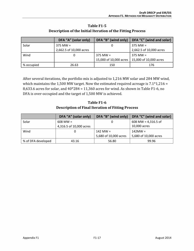
Assume a target generation capacity of 1,500 MW is required from three different but
equally sized DFAs, each of 10,000 acres. In this theoretical example DFA “A” can support
solar only; DFA “B” can support wind only; and DFA “C” can support both wind and solar.
The potential area available for solar is 20,000 acres (DFA “A” + DFA “C”); and the potential
area available for wind is 20,000 acres (DFA “B” + DFA “C”).
With no assumptions as to technology mix, the initial technology ratio is 1:1 (i.e., 750 MW
solar and 750 MWs wind). Consequently, the initial estimated acreage required to achieve a
1:1 mix would be 7.1*750 = 5,325 acres for solar, plus 40*750 = 30,000 acres for wind. As
is evident, this would require 35,325 acres, or 5,325 acres more than is available. However,
we continue with this example to illustrate the process.
If on average any acre in DFA “A” or DFA “C” is equally likely to be developed for solar (as a
consequence of rule 2 in Table F1-4), then the MWs developed will be directly proportional
to the size of the DFA. For example, for DFA “A” the proportion of MWs developed would be
0.5 (10,000 acres/20,000 acres = 0.5). Therefore, on average 0.5*750 = 375 MW of solar
development will occur in DFA “A”, and on average 0.5*750 = 375 MW of solar
development will occur in DFA “C”; the same assumptions hold true for wind.
If the required acreage is evaluated relative to the available acreage, the outcome is as
described in Table F1-5. Namely, 150% of the acres available in DFA “B” would be required
and 176% of the acres available in DFA “C” would be required. The distribution fails as it is
clearly impossible to use more land than is available in the DFA given the assumption that a
particular acre can only be occupied by a single resource type (Table F1-4, rule 3).
In order to satisfy the mutual exclusivity rule described in Table F1-4, rule 3, achieve the
target MWs, and maintain unbiased competition, the wind MWs are reduced.
Draft DRECP and EIR/EIS APPENDIX F1. METHODS FOR MEGAWATT DISTRIBUTION
Appendix F1 F1-17 August 2014
Table F1-5
Description of the Initial Iteration of the Fitting Process
DFA “A” (solar only) DFA “B” (wind only) DFA “C” (wind and solar)
Solar 375 MW =
2,662.5 of 10,000 acres
0 375 MW =
2,662.5 of 10,000 acres
Wind 0 375 MW =
15,000 of 10,000 acres
375 MW =
15,000 of 10,000 acres
% occupied 26.63 150 176
After several iterations, the portfolio mix is adjusted to 1,216 MW solar and 284 MW wind,
which maintains the 1,500 MW target. Now the estimated required acreage is 7.1*1,216 =
8,633.6 acres for solar, and 40*284 = 11,360 acres for wind. As shown in Table F1-6, no
DFA is over-occupied and the target of 1,500 MW is achieved.
Table F1-6
Description of Final Iteration of Fitting Process
DFA “A” (solar only) DFA “B” (wind only) DFA “C” (wind and solar)
Solar 608 MW =
4,316.5 of 10,000 acres
0 608 MW = 4,316.5 of 10,000 acres
Wind 0 142 MW =
5,680 of 10,000 acres
142MW =
5,680 of 10,000 acres
% of DFA developed 43.16 56.80 99.96

Draft DRECP and EIR/EIS APPENDIX F1. METHODS FOR MEGAWATT DISTRIBUTION
Appendix F1 F1-18 August 2014
Box 3
Formal Description of Method
The process optimizes the generation portfolio and its distribution by varying the
values of factor x such that the final technology portfolio and distribution between DFAs
satisfies the following:
∑ ∑ ( ( ))
Such that for all cases of p ∑
(4)
Where (3)
And
∑
(5)
And Technology specific area per MW
(i.e., solar and DG = 7.1; wind =40; geothermal = 5) (6)
And Siting discount factor for polygon p
(i.e., the siting discount factor ranging between 2 and 10 related to DFA sub-
areas). (7)
i = the ith iteration of the fitting process
n = final iteration of fitting process
p = indices of polygon p, being a defined sub-set of all available Development Focus Areas
m= maximum indices of p
x = a unitless factor iteratively fitted to satisfy the target
t = indices of technology type (i.e., solar, wind, geothermal)
Ap = Total Area of polygon p
Apt = Area of polygon p utilized by technology t
Apsolar = Area of polygon p utilized by solar
Apwind = Area of polygon p utilized by wind
Apgeo = Area of polygon p utilized by geothermal
MWpt = MWs of the tth technology assigned to polygon p
MWt = Total MWs of technology t

Draft DRECP and EIR/EIS APPENDIX F1. METHODS FOR MEGAWATT DISTRIBUTION
Appendix F1 F1-19 August 2014
F1.7 Combining the Scenarios
The main aim of combining scenarios was to provide maximum flexibility, and create
plausible aggregated scenarios that had the flexibility to deal with potential development
aggregation in different DRECP subareas. The combined scenario drew together the
maximum values for each technology in each of the DFA subsets. The method used a
bottom-up approach that took the maximum values for private, BLM, CSLC, and other
public lands identified for each technology in each ecoregional subareas and combined
them up into values for specific subareas and then up into the whole Plan Area. Table F1-7
illustrates this bottom-up approach using selected subregions of the DRECP; the values in
the input scenarios that feed into the final the aggregated scenario are highlighted. As is
evident in Table F1-7, the final scenario draws from different scenarios for different
regions and different jurisdictions to make up the final scenario. In particular, it is evident
that the maxima for public (BLM and CSLC) draw from different scenarios when compared
to the maxima for private (county and city jurisdiction) lands. Upon further review,
additional post hoc reduction of 20% to Imperial Borrego Valley subarea values was
considered necessary to ameliorate concerns about transmission constraints and reduce
likely impacts to prime agricultural land.
F1.8 Literature Cited
Dudek. 2012. Overview of DRECP Alternatives: Briefing Book 2. Prepared for the Renewable
Energy Policy Group. July 10, 2012.
Mahmoud, M., Liu Y., Hartmann, H., Stewart, S., Wagner, T., Semmens, D., Stewart, R., Gupta,
H., Dominguez, D., Dominguez, F., Hulse, D., Letcher, R., Rashleigh, B., Smith, C.,
Street, R., Ticehurst. J., Twery, M., van Delden, H., Waldick, R., White, D., Winter, L.
2009. “A Formal Framework for Scenario Development in Support of Environmental
Decision-Making.” Environmental Modeling and Software 24:798–808.
TTG (Transmission Technical Group), Dudek, and California Energy Commission. 2012.
Transmission Impacts in the DRECP. April 2012.
TTG. 2012. DRECP Transmission Technical Group Report: Conceptual Transmission Plan for
DRECP Alternatives. December 11, 2012.

Draft DRECP and EIR/EIS APPENDIX F1. METHODS FOR MEGAWATT DISTRIBUTION
Appendix F1 F1-20 August 2014
INTENTIONALLY LEFT BLANK

Draft DRECP and EIR/EIS APPENDIX F1. METHODS FOR MEGAWATT DISTRIBUTION
Appendix F1 F1-21 August 2014
Table F1-7
Sample of Information Flow from Input Scenarios to Aggregated Scenario Used for Estimating Generation Impacts

Draft DRECP and EIR/EIS APPENDIX F1. METHODS FOR MEGAWATT DISTRIBUTION
Appendix F1 F1-22 August 2014
INTENTIONALLY LEFT BLANK