Our Joint Future: Rural-Urban Interdependence in 21st Century Ohio

By

Mark D. Partridge

C. William Swank Chair in Rural-Urban Policy Professor, Agricultural, Environment, and Development Economics

Ohio State University

Jill Clark Agricultural, Environment, and Development Economics

Ohio State University

July 15, 2008

White Paper Prepared for the Brookings Institution

DDRRAAFFTT

  1

Executive Summary As we move into the 21st century, Ohio continues to struggle with economic restructuring and global competition. These struggles make it imperative to recognize that our economic engines link urban and rural Ohio—and all the suburban and exurban communities in between. This discussion paper examines the state’s geography of urban and rural interdependencies. We demonstrate that all Ohioans share a joint future that needs to be properly managed to ensure a prosperous tomorrow. The following are highlights from this discussion paper: 1.0 Introduction—Why Do All Ohioans have a Shared Fate?

• Ohio’s economy is lagging the nation and has done so since the late 1960s. • Ohio’s population growth is also lagging the nation and its peers, other Great Lake States.

At the same time, Ohioans are moving across the landscape, exurbanizing once rural areas.

• In a state with sixteen major metropolitan areas, Ohio’s underperformance is not just a problem for urbanites, but also for the suburban, exurban and rural residents that depend on these urban areas for economic growth and quality of life.

• If Ohio cannot compete on the national or international stage, communities both urban and rural (and suburban and exurban) will suffer together.

• Several factors illustrate the linkages between communities on the urban to rural spectrum, with the most obvious being the rural to urban (and urban to rural) movements of workers seeking out livelihoods across Ohio—in other words, commuting. But there are other linkages, such as use of retail, specialized services, educational instruction, and recreation opportunities that tie Ohio’s communities, functionally together.

2.0 Progress Report on Ohio’s Performance

• Ohio has even consistently lagged the nation and the other Great Lakes states in terms of job growth. We compare Ohio to its Great Lakes neighbors because they also facing many of the same impediments.

• A common explanation for Ohio’s underperformance is its manufacturing intensiveness. Ohio’s manufacturing is not the massive giant it once was and it is less likely to dramatically impact the state’s economy. Further, all Great Lakes states suffered from the restructuring of American manufacturing, but these states have generally outperformed Ohio.

• Global competition is also insufficient to explain Ohio’s difficulties. • Dismal income growth has been hand-in-hand with anemic job growth. In the mid-1950s

Ohio was ahead of the national average for income. In 2006, Ohio was 8 percent below the national average income.

3.0 The Geography of Ohio’s Populated Landscape

• Visually, the Ohio landscape takes on many forms along the urban to rural spectrum, but looks can be deceiving. The use and function of the landscape better explain the interdependencies between Ohio’s urbanites, suburbanites, exurbanites, and rural

  2

dwellers. • The U.S. Census Bureau has divided regions into metropolitan—nonmetropolitan to

reflect economic connections and urban-rural to reflect population densities. • Defining exurbia combines proximity to urban areas and lower population density. • The clear pattern of Ohio settlement is that virtually the entire state’s population lives

within a one hour’s drive of an urbanized area and are reliant on the associated jobs, services, and recreational venues—as well as the associated economic spillovers from these cities.

• Over half of Ohioans live within 10 miles of an urbanized area center. However, while Ohioans are close to urbanized areas, but tend not to live in them.

• 85 percent of Ohioans that reside in what the Census Bureau refers to as “rural” actually live in metropolitan or micropolitan areas.

• Nearly 30 percent of Ohioans, or 3.7 million, live in exurban areas. • While Ohio’s population has only slightly increased since 1970, the population has

become more dispersed across the landscape. This sprawling pattern also illustrates the geographically large “city-centered” regions that underlie the development of Ohio and most of the developed world.

4.0 Interdependencies Across Ohio’s Landscape

• Past research has demonstrated economic prosperity (or economic decline) is experienced across an entire region because of the interdependences between a city and its suburbs and exurbs. And these interdependencies are dynamic (Leichenko, 2001).

• Employment is probably the most noticeable way that relative economic prosperity is shared across a city and its suburbs (and exurbs) (Holzer and Stoll, 2007).

• Central city decline can reach a tipping point where further decline becomes impossible to stem, with large negative implications for neighboring suburbs/exurbs (Bradbury et al., 1980; Voith, 1993 and 1998).

• Rappaport (2005) considers central city and suburban growth dating back to the early 20th century. Though Rappaport’s research suggests that central city prosperity is third in importance, the fact that overall metropolitan forces are the strongest determinant of suburban growth illustrates that central cities and suburbs share a joint fate

• Urban linkages do not stop at the metropolitan area boarder, but extend through Ohio’s rural areas.

• Far outside the cities, incomes earned from commuting to urban jobs help support other jobs in rural and exurban communities, such as for local retail establishments or rural businesses.

• To understand why many amenities and services, such as specialized retail, healthcare, and entertainment, locate in urban areas, two concepts are useful, agglomeration economies and demand thresholds. It is the density of Ohio’s major cities that translates into our diverse and specialized economies not found in rural areas.

• The overwhelming majority of Ohioans derive their livelihood from urban areas. • Case examples from the Lima, Zanesville, and Cincinnati metro regions illustrate these

linkages. For example, 35 percent of workers in Hamilton County (Cincinnati) travel in from other counties both within and outside of the Cincinnati metropolitan area.

• Urban areas rely on rural areas for recreation, and other rural services.

  3

5.0 Drivers of Interdependence

• People, goods, and resources move along the urban to rural spectrum. Likewise the problems and challenges that communities face are structural and systematic as well, meaning that one community’s problem in a region spills over into the broader region. Peer effect and spillovers inextricably link our urban across to the rest of its region.

• In addressing regional spillovers, one solution is getting communities to more closely collaborate in their broader regions.

• Racial and social inequities across a region cause wasted creative capacity (Blackwell et al. 2007).

• Another shared fate is the results of sprawl and the reduction of quality of life across the region.

• Ohio’s regions are filled with “fragmented economic voices” too often pit one small box against another small box for a zero-sum game of economic development.

• Quantifying spillovers across Ohio, evidence demonstrates that poverty rates and median housing values in one county are related to nearby counties.

• In addition, median home values and per capita income in one neighborhood are related to nearby neighborhoods.

6.0 Recommendations 1. Local governments should more effectively share revenue so that entire regions receive the benefits and pay the costs of development. The Metropolitan Council from Minnesota is one model to follow. 2. Streamline local governments and create more effective regional planning and economic development authorities. Indiana’s model for a study commission would be one way to begin a critical assessment. 3. As a way to grease the wheels of regional reforms, consider more effective state revenue sharing with Ohio’s regions after they have undergone needed reforms for more effective regional governance. 4. Provide state infrastructure funding on a regional basis. Infrastructure funds should be prioritized to projects that make entire regions more competitive rather than scattering money among individual communities.

  4

1.0 Introduction—Why Do All Ohioans have a Shared Fate? Ohio’s economy has sharply lagged the national average since the 1960s. Though there are exceptions, Ohio’s lagging performance is primarily concentrated in its metropolitan areas (Partridge et al., 2007b). The underperformance of the state’s urban regions is not just felt by residents of central cities or inner-suburbs, it also directly relates to the prosperity of the residents in the outer suburbs, exurbs, and rural Ohio. It is hard to argue that turning around Ohio’s economic prospects doesn’t begin with turning around its cities and that virtually all Ohioans would benefit. With the sluggish economic conditions, the state’s population growth has been modest at best. Yet, Ohioans are still spreading out across the landscape. This sprawling low-density development emanates from urban areas and ties new exurban areas to urban cores. Since 1970, population growth has been pushing into traditional rural regions creating new exurban areas. In areas within commuting range of Ohio’s urban centers of 50,000 or more people, low-population density exurban rural areas are estimated to have increased from 58 percent of the state’s land area to 72 percent in this thirty-year time period.1 These exurban rural areas also witnessed rapid population growth, increasing by 27 percent in total population between 1970 and 2000 (an increase of approximately 392,000 people), versus only 6.6 percent statewide. It is far from clear if this low density development is optimal from either an economic growth perspective or a quality of life perspective. In almost nowhere is the transformation away from a sharp rural versus urban divide to a finer continuum of urban/suburban/exurban rural more complete than Ohio. In a state of barely 40,000 square miles, it contains parts of 16 metropolitan areas and 28 micropolitan areas with few rural communities far from an urban area. In between are relatively remote rural and exurban communities that rely on their urban neighbors for a host of functions including employment, retail, healthcare, entertainment and cultural venues, and business services. To illustrate this interdependence, we will focus on commuting and employment linkages because a person’s livelihood is arguably the most important feature of this interdependence. Moreover, commuting behavior is closely associated to accessing other urban services such as retail or healthcare. We will also consider other linkages including poverty and housing values. All Ohioans are interlinked to the prosperity of our cities. Many suburban, exurban, and rural Ohioans still ask why they should care about the prospects of the core principal cities (or the central city) and inner-tier suburbs. These non-central-city residents often believe that problems in the central cities are not really their concern. Though it is more accepted that more proximate suburbs and central cities are closely linked, economic transformation and technological change has produced the situation where almost all of Ohio’s exurban and rural communities are also part of far-reaching city-centered regions that compete on the national and international stage. This global competition of city-centered regions means that it is no longer the case (if it ever was) that (say) the Columbus region only competes with other Ohio cities such as Cincinnati, and that being more prosperous than other cities in the state is “good enough.” If the state’s city-regions are not competitive on a national or international basis, Ohioans—rural and urban alike—would be brought down together.

  5

It is well accepted that suburban residents have some linkage to their central city neighbor, but why do urban and nearby rural residents share the same fate? Specifically, up until the 1950s, rural communities were economically isolated from their city and suburban neighbors. Their residents were mostly employed in natural-resource dependent industries such as mining and agriculture or in industries with close ties to that sector. Yet, natural resource industries have undergone remarkable technological transformations in which they employ considerably fewer workers who are more productive and are usually better off than ever before. Today, many rural and exurban residents now commute and shop in other locations, most prominently to urban areas. For other reasons including environmental protection and recreation, urban residents are also interlinked with their rural and exurban neighbors. The upshot is the rise of interconnected regions that are centered on America’s urban metropolitan areas. These far-reaching regions can extend well outside the official metropolitan area boundaries in terms of these interdependencies. These interdependencies also illustrate why Ohio needs to think more regionally about its problems rather than locally. Much of our discussion will focus on the dependence of remote rural, exurban, and suburban communities on urban areas, including the core principal cities. Yet, our description would be incomplete without recognizing that the interdependence also goes the other way. Urban communities depend upon exurban and rural areas for a host of needs including a rural labor force, food, natural resources, environmental quality, recreation, tourism, markets for their products, and, in some cases, urban residents’ employment in rural and exurban communities. Indeed, the point of our assessment is that separating urban from rural is often pointless as healthy and prosperous rural and urban communities rely on the strength of their neighbors to succeed. In the ensuing discussion of how rural and urban communities are mutually interdependent, we will discuss the following: 1) Provide an overview of Ohio’s struggling economic performance. Then illustrate why some popular explanations are insufficient in explaining this subpar performance. Our point will be that systemic change is necessary if we hope for Ohio’s city-regions to become more internationally competitive. 2) Describe the geography of Ohio’s population settlement. 3) Provide a brief review of past research that illustrates how urban economic growth spills out and raises rural/suburban growth for about 100 miles from the urban center. 4) We then illustrate the rural-urban dependence in Ohio—primarily showing how commuting into urban centers is an important engine of growth for these outer communities. Then we describe other forms of rural-urban interdependencies such as recreation, infrastructure, business services, etc. and how they affect local governments. 5) We discuss how interdependence is driven by close proximity and spillovers across the landscape. These interdependencies indicate that Ohio’s current fragmented governance is inadequate in addressing 21st century realities. 6) Provide some policy suggestions aimed at improving the state’s economic conditions and describe a need for a new rural-urban compact toward a better shared governance across Ohio’s regions. 2.0 Progress Report on Ohio’s Performance

  6

Figure 1. Percentage Change in Total Employment in the United States, Ohio and the Great Lakes (less OH)

Since colonial settlement, America’s states and communities have faced periodic booms and busts as trading patterns changed or emerging technologies made an existing industry obsolete. Examples of economic downturns and creative destruction are well known including the decline of “King Cotton” in the 19th century American South, the closing of textile mills in New England, or the complete restructuring of America’s Cold War industrial economy in the 1990s, which primarily affected the coasts. The common story of American economic geography is that most places bounce back from these economic shocks. For instance, even smaller communities that faced significant military base closures in the late 1980s and early 1990s have tended to be no worse off today than when their base was open (Poppert and Herzog, 2003). Like most states, Ohio has also faced periodic economic distress. So we ask how has Ohio fared in the face of its own version of economic restructuring? We conclude, not very well. Ohio’s job growth has consistently lagged the nation and even other Great Lakes states. Along with the U.S., we compare Ohio to its Great Lakes state neighbors: Michigan, Indiana, Illinois, and Wisconsin because they share a common history and culture including a long-term dependence on manufacturing.2 These neighbors also share similar weather, which would lead to relative economic difficulties with respect to Sun Belt states that attract northern migrants. For these reasons, Ohio’s neighbors are also facing many of the same impediments and lagging these states would further suggest more systemic problems.

  7

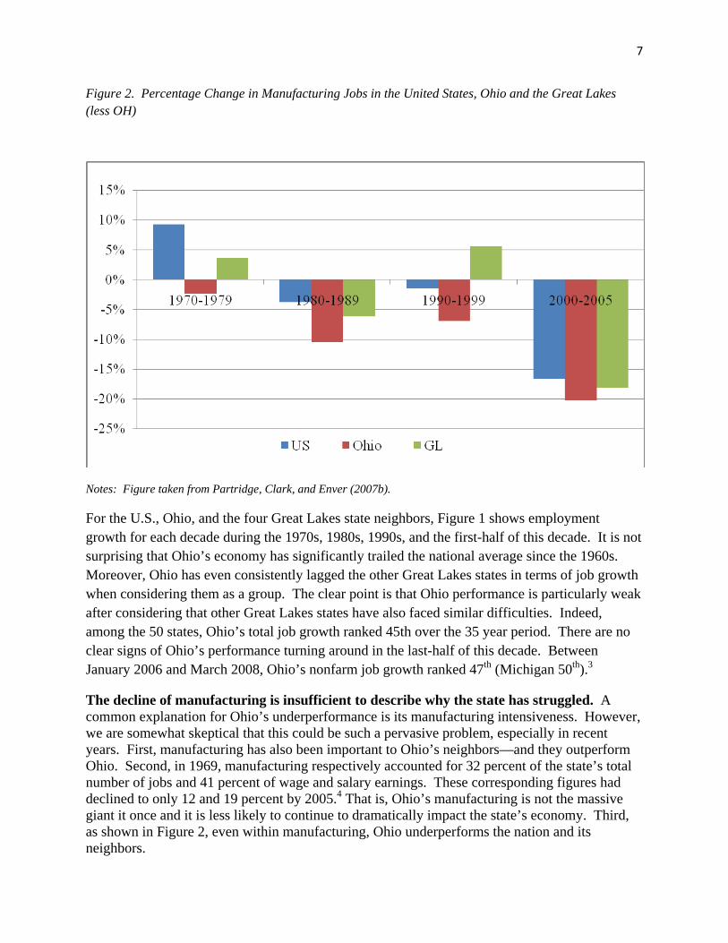
Figure 2. Percentage Change in Manufacturing Jobs in the United States, Ohio and the Great Lakes (less OH)

Notes: Figure taken from Partridge, Clark, and Enver (2007b).

For the U.S., Ohio, and the four Great Lakes state neighbors, Figure 1 shows employment growth for each decade during the 1970s, 1980s, 1990s, and the first-half of this decade. It is not surprising that Ohio’s economy has significantly trailed the national average since the 1960s. Moreover, Ohio has even consistently lagged the other Great Lakes states in terms of job growth when considering them as a group. The clear point is that Ohio performance is particularly weak after considering that other Great Lakes states have also faced similar difficulties. Indeed, among the 50 states, Ohio’s total job growth ranked 45th over the 35 year period. There are no clear signs of Ohio’s performance turning around in the last-half of this decade. Between January 2006 and March 2008, Ohio’s nonfarm job growth ranked 47th (Michigan 50th).3

The decline of manufacturing is insufficient to describe why the state has struggled. A common explanation for Ohio’s underperformance is its manufacturing intensiveness. However, we are somewhat skeptical that this could be such a pervasive problem, especially in recent years. First, manufacturing has also been important to Ohio’s neighbors—and they outperform Ohio. Second, in 1969, manufacturing respectively accounted for 32 percent of the state’s total number of jobs and 41 percent of wage and salary earnings. These corresponding figures had declined to only 12 and 19 percent by 2005.4 That is, Ohio’s manufacturing is not the massive giant it once and it is less likely to continue to dramatically impact the state’s economy. Third, as shown in Figure 2, even within manufacturing, Ohio underperforms the nation and its neighbors.

  8

It should also be noted that related explanations that revolve around manufacturing are insufficient to explain Ohio’s lagging performance. Many argue that the crisis in the domestic auto industry underlies Ohio’s problems. However, as Partridge et al (2007b) describe, the automobile manufacturing employment share only declined by about 0.5 percentage points in Ohio between 1999 and 2005.5 This is clearly insufficient to explain the sharp underperformance in the state, let alone answer the question as to why Ohio has not rebounded when other states have rebounded from past economic restructuring. Many Ohioans have surely suffered with the decline of the state’s manufacturers, but focusing solely on manufacturing draws attention away from other pressing causes for the state’s underperformance. While virtually all states have faced episodic declines in base economic sectors, what stands out for Ohio is its inability to redefine itself from a mid 20th century manufacturing juggernaut to a 21st century knowledge-economy leader. Successful regions throughout the world are able to adjust with the ebbs and flows of shifting competitive advantage. Restoring Ohio’s prosperity will require similar adjustments. Global competition is also insufficient to explain Ohio’s difficulties. There are others that argue that Ohio has taken a fierce beating from ever increasing global competition. Such an argument would be more convincing if the timing was right. For example, the U.S. did not start experiencing current account deficits until the early 1980s, well after Ohio’s relative decline began in the late 1960s. Similarly, NAFTA was not even ratified until 1993. Likewise, the rise and importance of Chinese imports is a 21st century phenomenon, again decades after Ohio’s difficulties began. The moral is that successful regions find ways to leverage globalization for its own prosperity rather than trying to cling to the past.6 Ohio also struggles in terms of income growth. In the mid 1950s, Ohio’s per capita income was almost 10 percent above the national average, falling to 8 percent below the national average by 2006 (Partridge et al. 2007b). If Ohio would just return to the national average, that would be consistent with about $12,000 more income for a family of four. The additional income could support extra government services such as healthcare, education, or improved infrastructure, with money to spare for other private and social needs. Ohio’s job growth especially lags in its metropolitan areas. Partridge et al. (2007b) find that Ohio’s metropolitan job growth is considerably weaker compared to metro job growth in the U.S. and in the other Great Lakes states. Conversely, nonmetropolitan Ohio’s job growth fares relatively better, and it even exceeded the growth rate of the U.S. and other Great Lakes states in the 1990s. Ohio’s urban job woes translate into much slower population growth. Partridge et al. (2007a) divided the nation’s metropolitan areas into three population-size groups and examined population growth over the 2000 to 2005 period. With the exception of Columbus, which is near the middle of its large metropolitan area grouping, all of the state’s metropolitan areas are near the bottom of their respective grouping.7 It is hard to fathom a scenario where Ohio dramatically improves its relative dismal performance without a dramatic improvement in its core cities and broader metropolitan areas. Yet, without that improved performance, Ohio will continue to be

  9

viewed as a less promising place for new investment and for entrepreneurs—further feeding a vicious cycle. In a global economy, financial capital, knowledge workers and entrepreneurs are attracted to places that are strongly performing because such places present fewer downside risks. Thus, changing these urban dynamics will create new opportunities for all of the state’s citizens. After describing the state’s populated landscape, the following sections illustrate why all Ohioans—rural and urban alike—would benefit from reinventing Ohio’s urban areas. Of course, city dwellers can immediately see the benefits, but the gains of shared prosperity will spread to the suburbs and countryside through greater jobs, which in turn support a healthier economy and higher quality of life. The renewed prosperity will allow state and local governments room to target more resources and investments to benefit all Ohioans. 3.0 The Geography of Ohio’s Populated Landscapes One of the key reasons for some observers to fail to recognize the degree of integration in Ohio’s regional economies is that the landscape may give a misleading impression of what the people are actually doing. For example, the suburban landscape may hide the interconnectedness with the core principal city. Likewise, the countryside may look very rural and bucolic, but the people who reside in these rural areas shop, recreate, and very often work in the nearby urbanized area. Understanding what the people are doing rather focusing on landscape or land use patterns underlies the broad interdependencies that we are considering. What follows in this section, is in two parts. The first part outlines the different ways to define rural and exurban Ohio. Foremost, this section reinforces how trying to draw a line between urban and rural is a challenging undertaking (if not impossible). But we do this so that we can precisely describe the state’s settlement pattern in the second subsection. 3.1 Defining Rural and Exurban Ohio When trying to grapple with describing the “urban-ness” or “rural-ness” of a place, some of the more commonly used terms from the US Census Bureau8 are metropolitan and nonmetropolitan (focusing on economic connections), and urban and rural (focusing on population density). We first describe these terms because of the frequency of which they are used. However, not only researchers, but those in the popular media, have recognized that the economic and social landscape is no longer a dichotomous (or either/or) urban versus rural. As a result, notions of varying community types along a spectrum have been introduced. Therefore, we next discuss geographies along a rural-urban continuum, using both economic connectedness and population density. Metropolitan vs. Nonmetropolitan. This dichotomous approach of metropolitan vs. nonmetropolitan has recently been expanded to include micropolitan, a subset of nonmetropolitan, to attempt to better demonstrate differing types of urban agglomerations. This approach relies on counties as the boundaries. Figure 3 illustrates how this categorization is used on the Ohio landscape.

  10

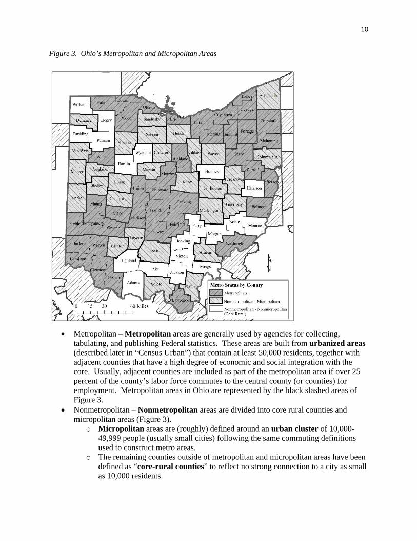
Figure 3. Ohio’s Metropolitan and Micropolitan Areas

• Metropolitan – Metropolitan areas are generally used by agencies for collecting,

tabulating, and publishing Federal statistics. These areas are built from urbanized areas (described later in “Census Urban”) that contain at least 50,000 residents, together with adjacent counties that have a high degree of economic and social integration with the core. Usually, adjacent counties are included as part of the metropolitan area if over 25 percent of the county’s labor force commutes to the central county (or counties) for employment. Metropolitan areas in Ohio are represented by the black slashed areas of Figure 3.

• Nonmetropolitan – Nonmetropolitan areas are divided into core rural counties and micropolitan areas (Figure 3).

o Micropolitan areas are (roughly) defined around an urban cluster of 10,000-49,999 people (usually small cities) following the same commuting definitions used to construct metro areas.

o The remaining counties outside of metropolitan and micropolitan areas have been defined as “core-rural counties” to reflect no strong connection to a city as small as 10,000 residents.

  11

Figure 4. Example of Ohio’s Metro/Micro and Urban/Rural Geography

census rural

census urban

Note that metro areas are officially defined on the basis of what the people are doing and not necessarily by the nature of the landscape. The landscape may be (say) farming, but the county would still be part of a metropolitan area if its residents are significantly linked to the central core through economic and social interactions. Thus, in terms of measuring interdependence, the definition of metropolitan areas best fits our needs. However, metropolitan areas present an either/or choice and does not allow for the idea that development and use occurs on a continuum. We attempt to address this issue later in this section. Urban vs. Rural. Another categorization is the U.S. Census Bureau’s official definition of “Census Urban” and “Census Rural.” These geographies are built from census blocks. Figure 4 provides an example of these definitions for metropolitan Columbus—e.g., it shows urbanized areas around Columbus and Newark as well as urbanized clusters around Lancaster, Circleville, etc. combining both metro/nonmetro and urban/rural.

• Census Urban – Census Urban refers to high population densities consisting of a large central place and adjacent densely settled census blocks. When urban census blocks are considered together as a collective, they are either urbanized areas or urban clusters.

o Urbanized areas – Generally, we will refer to “urbanized areas” as entire urban

  12

concentrations that include a ‘core principal’ or ‘central’ city (cities). So for Cleveland’s urbanized area, the urbanized area would refer to the core principal city of Cleveland and the surrounding suburbs with high population densities.

o Urban cluster – Urban clusters that together have a total population of at least 2,500 for urban clusters, or at least 50,000 for urbanized areas. The urban definition essentially includes areas of at least 1,000 people per square mile along with any adjacent areas with at least 500 people per square mile. Urban is divided into urbanized clusters (usually towns and cities) with between 2,500 and 50,000 residents and urban areas (usually cities) greater than 50,000. Urban classification cuts across other hierarchies and can be in metropolitan or non-metropolitan areas.

• Census Rural – Census Rural includes territory, population and housing units not classified as urban. Rural classification cuts across other hierarchies and can be in metropolitan or non-metropolitan areas.

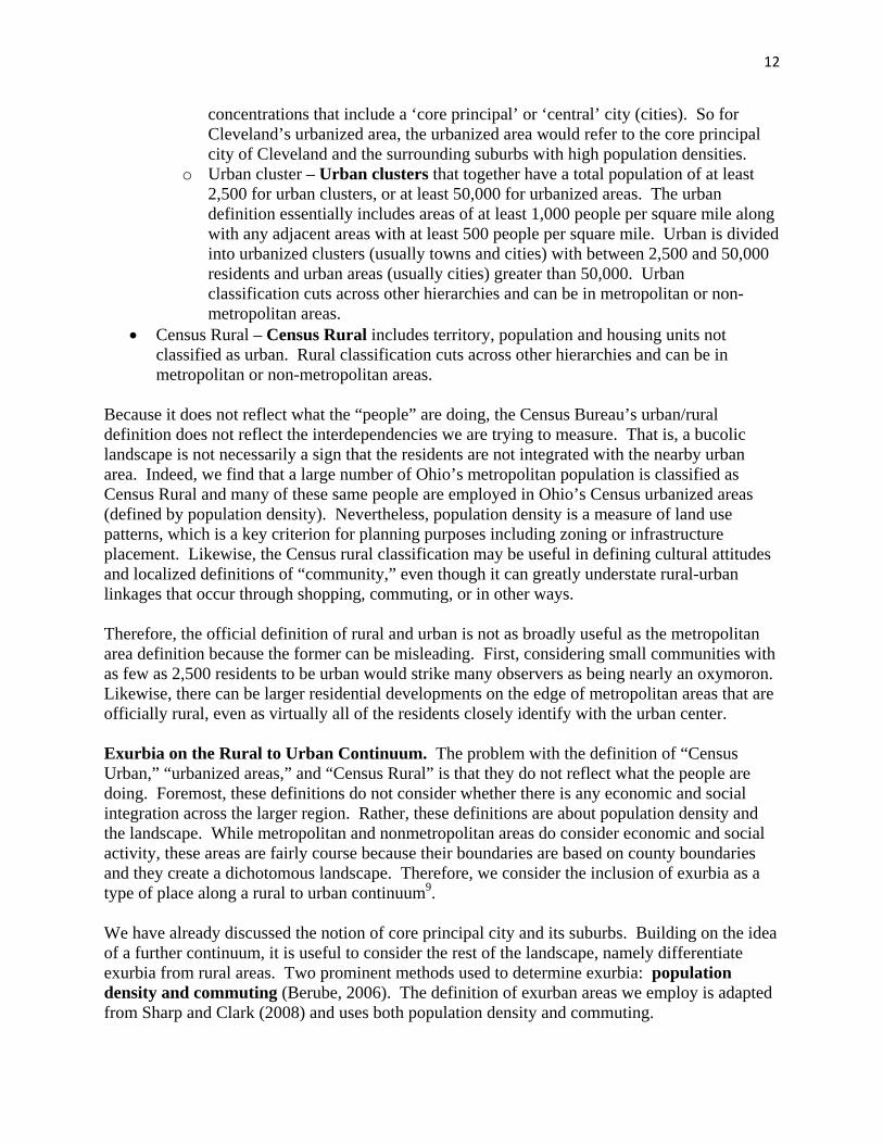
Because it does not reflect what the “people” are doing, the Census Bureau’s urban/rural definition does not reflect the interdependencies we are trying to measure. That is, a bucolic landscape is not necessarily a sign that the residents are not integrated with the nearby urban area. Indeed, we find that a large number of Ohio’s metropolitan population is classified as Census Rural and many of these same people are employed in Ohio’s Census urbanized areas (defined by population density). Nevertheless, population density is a measure of land use patterns, which is a key criterion for planning purposes including zoning or infrastructure placement. Likewise, the Census rural classification may be useful in defining cultural attitudes and localized definitions of “community,” even though it can greatly understate rural-urban linkages that occur through shopping, commuting, or in other ways. Therefore, the official definition of rural and urban is not as broadly useful as the metropolitan area definition because the former can be misleading. First, considering small communities with as few as 2,500 residents to be urban would strike many observers as being nearly an oxymoron. Likewise, there can be larger residential developments on the edge of metropolitan areas that are officially rural, even as virtually all of the residents closely identify with the urban center. Exurbia on the Rural to Urban Continuum. The problem with the definition of “Census Urban,” “urbanized areas,” and “Census Rural” is that they do not reflect what the people are doing. Foremost, these definitions do not consider whether there is any economic and social integration across the larger region. Rather, these definitions are about population density and the landscape. While metropolitan and nonmetropolitan areas do consider economic and social activity, these areas are fairly course because their boundaries are based on county boundaries and they create a dichotomous landscape. Therefore, we consider the inclusion of exurbia as a type of place along a rural to urban continuum9. We have already discussed the notion of core principal city and its suburbs. Building on the idea of a further continuum, it is useful to consider the rest of the landscape, namely differentiate exurbia from rural areas. Two prominent methods used to determine exurbia: population density and commuting (Berube, 2006). The definition of exurban areas we employ is adapted from Sharp and Clark (2008) and uses both population density and commuting.

  13

Figure 5. Ohio’s Exurban Geography

Given the great range in sizes of the state's urbanized areas, commuting times were anticipated to vary according to the population of the urbanized area. Analysis of commuting data verified this expectation, with average commutes longer around the largest urbanized areas and shorter around the smallest. To account for this variation, the commuting field was defined as 35 miles from the edge of the largest urbanized areas (one million or more residents); 25 miles from the edge of urbanized areas with a population between 500,000 and one million people; and 15 miles from the edge of urbanized areas of less than 500,000 residents. Results are shown in Figure 5. Then in these easily commutable areas shown in Figure 5, we define exurban densities as Census Rural areas with population densities greater than 40 people per square mile. In

  14

Figure 6. Population Density Change in Ohio’s Landscape

1970 1990

Projected2010

Notes: Figure adapted from Irwin and Reece (2002).

Acres perHousing UnitSettlement Pattern People/sq. mi.

Urban High Density greater than 5,000 <1/3Urban Low Density 1000-5000 1/3 - 1.5

Exurban High Density 325-1000 1.5 - 5Exurban Low Density 40-325 5 - 40

Rural 0-40 greater than 40

  15

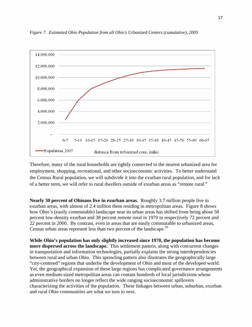
Figure 6 we further delineate exurban into high and low exurban densities by defining high-density exurban has having between 325 to 1,000 people per square mile and low-density exurban as having between 40 and 325 people per square mile. Therefore, the exurban landscape is differentiated between exurban and rural population densities, using the approach following Irwin and Reece (2002). This exercise allows us to examine a larger range of community types (other than urban versus rural) at the same time recognizing the economic ties between types. 3.2 Where do the roughly 11.5 million Ohioans live? This section focuses on examining the Ohio population in light of the ways of examining not just the urban-ness and rural-ness of the Ohio landscape, but also the ways these different populations are linked together across multiple functions and shared fates. Over 80 percent of Ohio’s population live in areas classified as “metropolitan” by the U.S. Census Bureau. Table 1 shows that as of 2000, over 81 percent of Ohio’s population resides in metropolitan areas, 15 percent in micropolitan areas and only 4 percent reside in core rural areas. Yet, 7.3 million or only 64 percent of Ohioans live in densely populated urbanized areas (principal cities and their suburbs). The remaining 36 percent live in smaller urbanized clusters and Census Rural areas including the 1.3 percent of Ohioans that reside on farms. Thus, over one-third of the state’s residents live in less populated communities. Over half of Ohioans live within 10 miles of an urbanized area center. Figure 5 shows the number of Ohioans that live within a given distance of the geographical center of one of one Ohio’s urbanized areas (roughly cities of at least 50,000 people). The figure shows that 5.9 million live within 10 miles of a geographical center, while 11.4 million (or 99 percent of Ohioans) live within 50 miles. The clear pattern is that virtually the entire state’s population lives within a one hour’s drive of an urbanized area and are reliant on the associated jobs, services, and recreational venues—as well as the associated economic spillovers from these cities. Ohioans are close to urbanized areas, but tend not to live in them. Even when Ohio’s metropolitan areas are examined in isolation, a surprisingly large share live outside of the core urbanized areas that form the center of the metropolitan areas. Specifically, among the 9.1 million Ohioans that reside within its metropolitan areas, about 80 percent (7.3 million) are in the densely population urbanized areas (Table 1). Another 482,000 residents live in smaller urbanized clusters of less than 50,000 (e.g., Medina near Cleveland or Delaware near Columbus). Moreover, nearly 1.4 million metropolitan Ohioans reside in Census rural areas. These include over 60,000 who live on farms, or over 40 percent of the state’s farm population resides in metropolitan areas. That is, a large share of Ohio’s farmers live in regions tightly integrated to larger principal cities and they have a clear stake in the quality of governance and quality/cost of associated public services. Urban and rural areas are distributed more evenly in Micropolitan counties. Again, an estimated 15 percent of Ohioans live in micropolitan counties (Table 1). An estimated 40 percent of the state’s farm population resides in micropolitan areas. In core rural areas, about 75

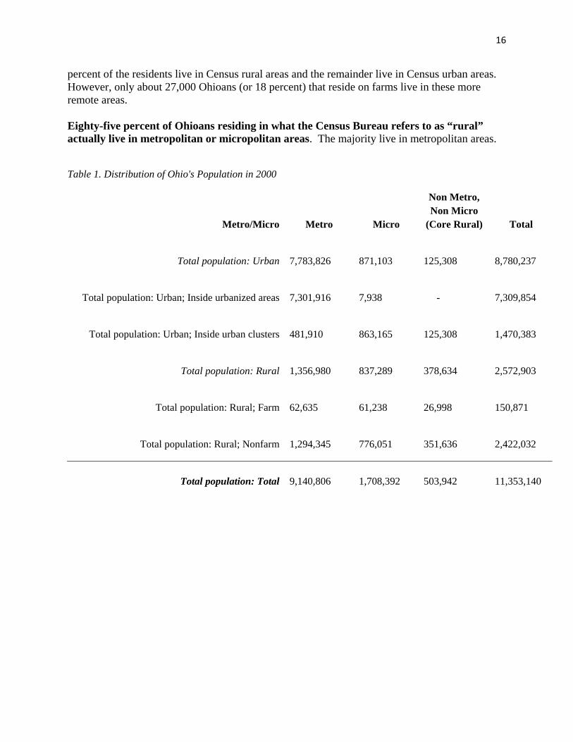
  16

percent of the residents live in Census rural areas and the remainder live in Census urban areas. However, only about 27,000 Ohioans (or 18 percent) that reside on farms live in these more remote areas. Eighty-five percent of Ohioans residing in what the Census Bureau refers to as “rural” actually live in metropolitan or micropolitan areas. The majority live in metropolitan areas.

Table 1. Distribution of Ohio's Population in 2000

Metro/Micro Metro Micro

Non Metro, Non Micro

(Core Rural) Total

Total population: Urban 7,783,826

871,103

125,308

8,780,237

Total population: Urban; Inside urbanized areas 7,301,916

7,938 -

7,309,854

Total population: Urban; Inside urban clusters 481,910

863,165

125,308

1,470,383

Total population: Rural 1,356,980

837,289

378,634

2,572,903

Total population: Rural; Farm 62,635

61,238

26,998

150,871

Total population: Rural; Nonfarm 1,294,345

776,051

351,636

2,422,032

Total population: Total 9,140,806

1,708,392

503,942

11,353,140

  17

Figure 7. Estimated Ohio Population from all Ohio's Urbanized Centers (cumulative), 2005

Therefore, many of the rural households are tightly connected to the nearest urbanized area for employment, shopping, recreational, and other socioeconomic activities. To better understand the Census Rural population, we will subdivide it into the exurban rural population, and for lack of a better term, we will refer to rural dwellers outside of exurban areas as “remote rural.”

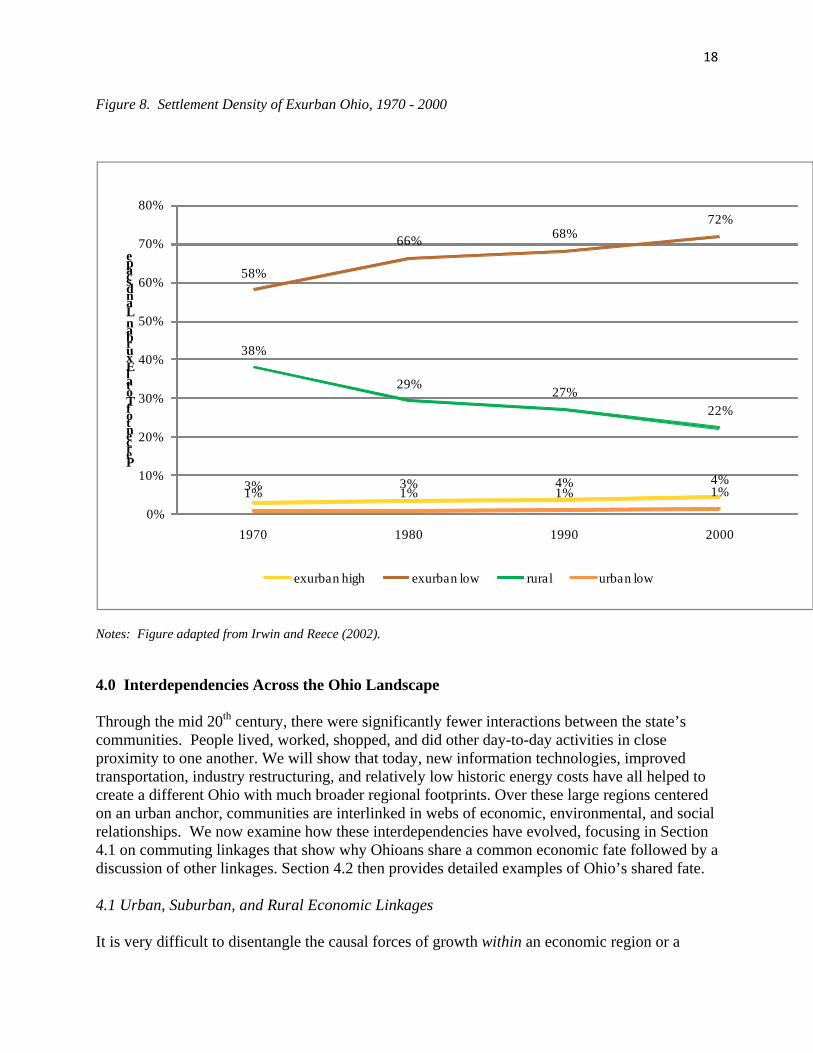
Nearly 30 percent of Ohioans live in exurban areas. Roughly 3.7 million people live in exurban areas, with almost of 2.4 million them residing in metropolitan areas. Figure 8 shows how Ohio’s (easily commutable) landscape near its urban areas has shifted from being about 58 percent low-density exurban and 38 percent remote rural in 1970 to respectively 72 percent and 22 percent in 2000. By contrast, even in areas that are easily commutable to urbanized areas, Census urban areas represent less than two percent of the landscape.10 While Ohio’s population has only slightly increased since 1970, the population has become more dispersed across the landscape. This settlement pattern, along with concurrent changes in transportation and information technologies, partially explains the strong interdependencies between rural and urban Ohio. This sprawling pattern also illustrates the geographically large “city-centered” regions that underlie the development of Ohio and most of the developed world. Yet, the geographical expansion of these large regions has complicated governance arrangements as even medium-sized metropolitan areas can contain hundreds of local jurisdictions whose administrative borders no longer reflect the wide ranging socioeconomic spillovers characterizing the activities of the population. These linkages between urban, suburban, exurban and rural Ohio communities are what we turn to next.

  18

Figure 8. Settlement Density of Exurban Ohio, 1970 - 2000

3% 3% 4% 4%

58%

66% 68%72%

38%

29% 27%22%

1% 1% 1% 1%

0%

10%

20%

30%

40%

50%

60%

70%

80%

1970 1980 1990 2000

Percent of Total Exurban Landscape

exurban high exurban low rural urban low

Notes: Figure adapted from Irwin and Reece (2002).

4.0 Interdependencies Across the Ohio Landscape Through the mid 20th century, there were significantly fewer interactions between the state’s communities. People lived, worked, shopped, and did other day-to-day activities in close proximity to one another. We will show that today, new information technologies, improved transportation, industry restructuring, and relatively low historic energy costs have all helped to create a different Ohio with much broader regional footprints. Over these large regions centered on an urban anchor, communities are interlinked in webs of economic, environmental, and social relationships. We now examine how these interdependencies have evolved, focusing in Section 4.1 on commuting linkages that show why Ohioans share a common economic fate followed by a discussion of other linkages. Section 4.2 then provides detailed examples of Ohio’s shared fate. 4.1 Urban, Suburban, and Rural Economic Linkages It is very difficult to disentangle the causal forces of growth within an economic region or a

  19

metropolitan area. The economic forces that affect a metropolitan area could originate across the entire metropolitan region, or from the principal city, or from the surrounding suburbs (or some combination of the three). For example, is the economic experience of a given metropolitan area— suburbs and central city—due to metro-wide forces that jointly shape both suburb and central city alike, or do the driving forces originate in either the central core or the suburbs?11 Of course, to some extent, all three forces likely play a role. Because they are all happening at once within very interconnected metropolitan areas, it becomes particularly difficult to identify the economic driver—and indeed—it may not matter as long as the entire metro area is prosperous. Employment is probably the most noticeable way that relative economic prosperity is shared across a city and its neighboring suburbs. Holzer and Stoll (2007), for example, find that there are significant commuting flows between the central city, low-income suburbs, and high-income suburbs. They find that about 30 percent of the central-city workforce commutes to the suburbs for employment. Indeed, during the 1990s, job growth was particularly brisk in high-income suburbs, while population grew the fastest in low-income suburbs (with high out-commuting from low- to high-income suburbs). Even when focusing on just the first-tier or inner suburbs, Puentes and Warren (2006) find tremendous diversity. Some inner suburbs are prosperous in terms of rising incomes and home values. Other inner suburbs are increasingly taking on the characteristics of their neighboring inner cities with increasing racial diversity, aging infrastructure, and more concentrated poverty. In some cases, without road signs, it is increasingly difficult when traveling along the streets to know when one crosses the boundary between a first-tier suburb and a principal city. In their examination of suburban-central city interdependence, Bradbury et al. (1980) note that central city decline can reach a tipping point where further decline becomes impossible to stem, with large negative consequences for neighboring suburbs. Avoiding such negative thresholds would be something that should unify all metropolitan residents. This pattern is consistent with Voith’s (1993; 1998) findings that a strong central city economy induces better suburban economic outcomes such as greater income growth and stronger housing prices. In particular, the linkage for housing prices is telling because property values are a forward-looking indicator, suggesting that market participants link the prosperity of the principal city with prosperity in the nearby suburbs. Yet, Leichenko (2001) finds that the interdependence between suburban and central city growth changes over time. While suburban growth was more likely to spur central city growth in the 1970s and 1980s, there was stronger joint determination in the 1990s. One of the most complete recent efforts in examining central city and suburban interdependence is Rappaport (2005). His study considers central city and suburban growth dating back to the early 20th century. Rappaport finds that the underlying causes of a given metropolitan area’s suburban growth can be attributed to the following three factors in declining importance: (1) the underlying metropolitan area’s growth dynamics, (2) the underlying trend for all American suburbs to grow at a relatively faster rate, and (3) growth spreading from a vibrant central city out to the suburbs. Though Rappaport’s research suggests that central city prosperity is third in importance, the fact that overall metropolitan forces are the strongest determinant of suburban growth illustrates that central cities and suburbs share a joint fate. They cannot decouple themselves from one another. If the metropolitan area is uncompetitive for business and/or lacks

  20

a sufficient quality of life to attract and retain population, both the suburbs and the central city will suffer (see Hill and Brennan, 2005 for a similar overview). Alternatively, steps that improve the competitiveness of the metropolitan area—whether concentrated in the suburbs or the central city—will benefit all of the metropolitan area’s residents. Extending far into the neighboring rural fringe, the influence of a given metropolitan area’s growth does not end at its border. As Partridge et al. (2007b) generally describe, almost all reaches of Ohio are affected by metropolitan and urbanized area job opportunities with significant shares of the rural and exurban workforce commuting and working in one of Ohio’s urbanized areas. This pattern is not unique to Ohio. There is a long-established rural development literature that examines whether urban growth “spreads” into the countryside or whether rural and urban growth are complementary (Kahn et al., 2001). For example, Henry et al. (1997) find that urban growth tends to spread to the nearby rural and exurban areas, though they note that there are differences depending on whether the urban-led growth originates in the core principal city or in the suburbs. Using Canadian data, Partridge et al. (2007a) find that urban income and population growth spreads into nearby rural areas for about 100 miles. Further supporting the view that rural areas are highly dependent on urban areas for economic growth, Partridge et al. (2008b) find that U.S. rural employment growth is strongly affected by proximity to the nearest urban center, which is also the case when examining rural wages and housing values (Partridge et al., 2008a). The latter two studies found that urban proximity is one of the strongest factors affecting rural economic outcomes. As we will show for Ohio below, the key way that growth in urbanized areas creates rural, exurban, and suburban opportunities is through commuting. Urban growth also helps stimulate demand for goods and services produced in nearby rural and exurban communities, such as for food and recreation (Henry et al., 1997). Likewise, ease in accessing other urban businesses services greatly enhances the competitiveness of rural and exurban businesses, while access to urban amenities has corresponding effects in enriching the lives of rural residents. In sum, far outside the cities, incomes earned from commuting to urban jobs help support other jobs in rural and exurban communities, such as for local retail establishments or rural businesses. Urban-based jobs help maintain a viable rural and exurban population base that facilitates community vitality (e.g., having enough students for schools, property & sales taxes, strong local businesses, etc). A sufficient critical mass is essential in maintaining vital rural communities and it does not matter if a significant share of the residential base is commuting elsewhere for employment. We should clarify the difference between healthy rural development and the more costly sprawling exurban development described elsewhere in this report. Specifically, when we are describing rural development in this section, we are talking about sensible development in established towns and villages—we are not advocating new sprawling developments into exurbia. In terms of lost green space, increased cost of public service delivery, greater gasoline usage, there are related reasons why Americans should be worried about expanding sprawl into exurban areas. Though urbanized areas are a key economic driver of these exurban areas, the prosperity of the principal city and inner suburbs can curb some of the expansion of the footprint of these exurban areas by promoting a reasonable share of residential development in the

  21

principal city (Kurban and Persky, 2007). A good mixture of both rural and urban is reliant on strong urban areas. Commuting, when livelihoods are sought in other places, is one clear example of linkages of use across communities, particularly when income is generated in one community and spent in another (perhaps the home community). But there are many other uses that cause movement of people across the rural-urban continuum to utilize amenities and services located outside of their community, such as urban amenities, rural recreation, and higher-ordered urban services. Why are cities centers of economic activity? To understand why many amenities and services locate in urban areas, two concepts are useful, agglomeration economies and demand thresholds. It is the location of these amenities and services in urban areas that are utilized by urbanites, suburbanites, exurbanites, and rural Ohioans alike. Businesses cluster in cities because of agglomeration economies. Agglomeration economies occur when firms locate near one another. Theoretically, the more that related firms are clustered together, the lower the costs of the production and the greater their market. Advantages of agglomerating include easier access to information and new and innovative ideas, and fixed costs might be lower, making production cheaper. The benefits of agglomeration are the facilitation of economic activity through factors such as access to specialized services; broader labor supply pools; lower transportation costs with suppliers, and with final customers; and ease in imitating successful rivals through knowledge spillovers. Ohio’s urban economies are a result of exploiting these agglomeration benefits – i.e., this is one reason why cities grow and have concentrations of economic activity. Examples of agglomeration economies in Ohio include Honda and its suppliers in near Marysville and Cleveland’s cluster of museums located in University Circle. Cities host the entire range of retail and services because large populations meet demand thresholds. Another factor in making locational decisions is the concept of demand threshold. Demand thresholds are simply the minimum level of population (and their income) required to support a service. Demand thresholds fall from the classic notion of Central Place Theory (Christaller, 1933) in which there is an urban system that begins with rural areas, rising all the way to largest cities. Consider the difference between trying to locate an appropriate community for a gas station (convenience goods), or a high-end shoe store (specialty good), or a national sports team (specialized event)? What drives these decisions regarding retail, healthcare, and others services such as hotels? Demand. And what drives demand? Population and income. So it is the density of Ohio’s major cities that translates into our diverse and specialized economies not found in rural and exurban areas. It also means that much of the urban infrastructure, such as communications and transportation, are located in urban areas to serve these economies. And it is the density of Ohio’s urban areas that enable agglomerations of higher-ordered services to occur. 4.2 Growth and Change in Ohio: Commuting Links Across the Ohio Landscape This section directly illustrates the interdependencies across Ohio’s landscape. Though these

  22

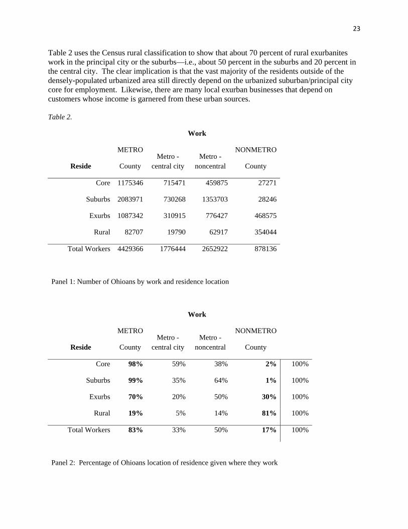
interdependencies are manifested in many dimensions, we will focus on place-of-resident and place-of-work data as best showing this interdependence. Some of the reasons for this decision include: (1) commuting clearly shows how a resident of one location engages in activities in multiple different locations; (2) though there are other activities such as air pollution or retail shopping that could also illustrate such spillovers, the key advantage of commuting data is it is widely available; and (3) because it involves the direct or indirect livelihood of much of the population, commuting significantly affects the well-being of the population. Indeed, using the commuting data described in Side Box 1, about 27 percent of Ohioans worked outside of their county of residence in 2000. A key trend is that there are about as many workers who reside in (Census Rural) exurban Ohio as there are workers who reside in the state’s core principal cities. Table 2 illustrates commuting patterns in 2000 for workers living in the core or principal city of Ohio’s 16 metropolitan areas, those who live in the suburbs (i.e., in the urbanized area outside of the principal city), in the rural exurbs, and in remote rural areas. The table also shows that 1.78 million Ohioans work in the principal core cities (summing down the first column), but only 1.2 million workers actually reside in the principal city (summing across the first row). This illustrates that Ohio’s principal cities are, on balance, major net jobs creators. Indeed, as the lower panel of Table 2 shows, only 40 percent of the principal-city workforce actually resides in the central (principal) city, while 41 percent originate from the suburbs, 18 percent is from the exurbs, and another 2 percent commute from nonmetro areas. Indeed, more suburbanites work in the principal/central city than principal cities residents. Seventy percent of rural exurbanites work in the principal city or the suburbs Panel 2 of

Side Box 1. Discussion of the Data Used in this report

Employment. The primary data source that we use for total employment—including the number self employed—is the U.S. Bureau of Economic Analysis, Regional Economic Information System. Data was available for the 1969-2005 period at the time of this writing (available at www.bea.gov). BEA data counts the number of jobs in a particular county (place of work). It does not count the number of employed residents. For example, if an individual has three part-time jobs located in a particular county, it is counted as three different jobs in that county regardless of the residence of the worker. The strength of BEA data is that it is very accurate because it is benchmarked to IRS tax returns, unemployment insurance data, and other sources. Another advantage is that it is annually available at the county level, which is not the case for most other employment sources.

Generally, regional economists prefer place-of-work data because it shows the economic conditions for a particular location. However, counting the number of jobs does come at the disadvantage of not capturing whether a significant share of these jobs are ‘casual,’ or for only a minimal number of hours. Place-of-resident data may reflect job patterns elsewhere due to in- and out-commuting. However, when we are trying to show interdependence, place of residence data does capture the intended commuting flows.   

Commuting. The commuting data we use is derived from two sources, the Census 2000 STF 3 data that can be downloaded from U.S. Census Bureau website using the American Fact Finder tool (www.census.gov) and USDA Economic Research Service Rural-Urban Commuting Area Codes (http://www.ers.usda.gov/briefing/Rurality/RuralUrbanCommutingAreas/). Likewise, the population data we utilize is also from the U.S. Census Bureau website under population estimates.

Business Locations. The locational data use for locations of malls, hospitals, and other venues in Figures 14 and 15 is from ESRI’s Business Analyst package (www.esri.com).

  23

Table 2 uses the Census rural classification to show that about 70 percent of rural exurbanites work in the principal city or the suburbs—i.e., about 50 percent in the suburbs and 20 percent in the central city. The clear implication is that the vast majority of the residents outside of the densely-populated urbanized area still directly depend on the urbanized suburban/principal city core for employment. Likewise, there are many local exurban businesses that depend on customers whose income is garnered from these urban sources. Table 2.

Work

Reside

METRO

County Metro -

central city Metro -

noncentral

NONMETRO

County

Core 1175346 715471 459875 27271

Suburbs 2083971 730268 1353703 28246

Exurbs 1087342 310915 776427 468575

Rural 82707 19790 62917 354044

Total Workers 4429366 1776444 2652922 878136

Panel 1: Number of Ohioans by work and residence location

Work

Reside

METRO

County Metro -

central city Metro -

noncentral

NONMETRO

County

Core 98% 59% 38% 2% 100%

Suburbs 99% 35% 64% 1% 100%

Exurbs 70% 20% 50% 30% 100%

Rural 19% 5% 14% 81% 100%

Total Workers 83% 33% 50% 17% 100%

Panel 2: Percentage of Ohioans location of residence given where they work

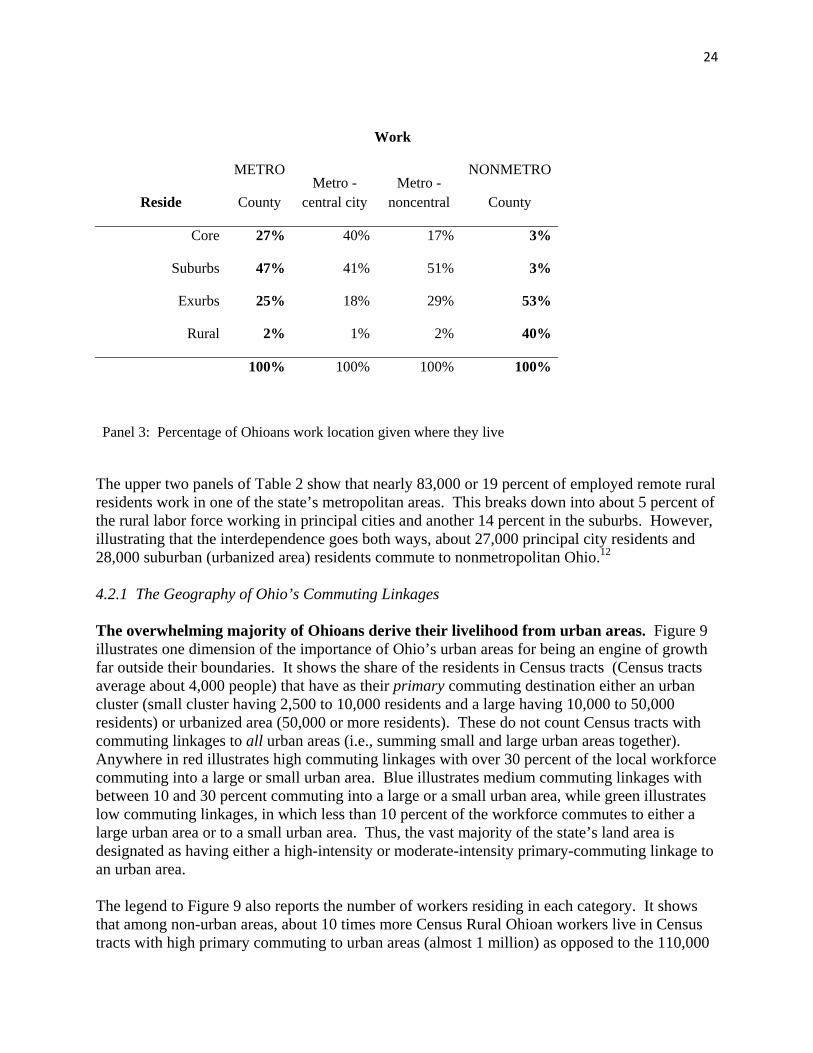
  24

Work

Reside

METRO

County Metro -

central city Metro -

noncentral

NONMETRO

County

Core 27% 40% 17% 3%

Suburbs 47% 41% 51% 3%

Exurbs 25% 18% 29% 53%

Rural 2% 1% 2% 40%

100% 100% 100% 100%

Panel 3: Percentage of Ohioans work location given where they live

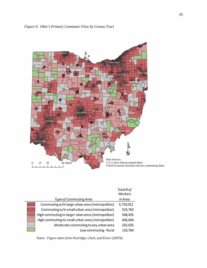
The upper two panels of Table 2 show that nearly 83,000 or 19 percent of employed remote rural residents work in one of the state’s metropolitan areas. This breaks down into about 5 percent of the rural labor force working in principal cities and another 14 percent in the suburbs. However, illustrating that the interdependence goes both ways, about 27,000 principal city residents and 28,000 suburban (urbanized area) residents commute to nonmetropolitan Ohio.12 4.2.1 The Geography of Ohio’s Commuting Linkages The overwhelming majority of Ohioans derive their livelihood from urban areas. Figure 9 illustrates one dimension of the importance of Ohio’s urban areas for being an engine of growth far outside their boundaries. It shows the share of the residents in Census tracts (Census tracts average about 4,000 people) that have as their primary commuting destination either an urban cluster (small cluster having 2,500 to 10,000 residents and a large having 10,000 to 50,000 residents) or urbanized area (50,000 or more residents). These do not count Census tracts with commuting linkages to all urban areas (i.e., summing small and large urban areas together). Anywhere in red illustrates high commuting linkages with over 30 percent of the local workforce commuting into a large or small urban area. Blue illustrates medium commuting linkages with between 10 and 30 percent commuting into a large or a small urban area, while green illustrates low commuting linkages, in which less than 10 percent of the workforce commutes to either a large urban area or to a small urban area. Thus, the vast majority of the state’s land area is designated as having either a high-intensity or moderate-intensity primary-commuting linkage to an urban area. The legend to Figure 9 also reports the number of workers residing in each category. It shows that among non-urban areas, about 10 times more Census Rural Ohioan workers live in Census tracts with high primary commuting to urban areas (almost 1 million) as opposed to the 110,000

  25

Figure 9. Ohio’s Primary Commuter Flow by Census Tract

 

Columbus

Cleveland

Cincinnati

Dayton

Lima

Toledo

Marietta

Akron

Newark

Athens

Canton

Youngstown

 

 

Total # of Workers

Type of Commuting Area in AreaCommuting w/in large urban area (metropolitan) 3,719,012 Commuting w/in small urban area (micropolitan) 523,763 

High commuting to larger ubanarea (metropolitan) 548,435 High commuting to small urban area (micropolitan) 436,644 

Moderate commuting to any urban area 235,635 Low commuting ‐ Rural 110,764 

       Notes: Figure taken from Partridge, Clark, and Enver (2007b).

  26

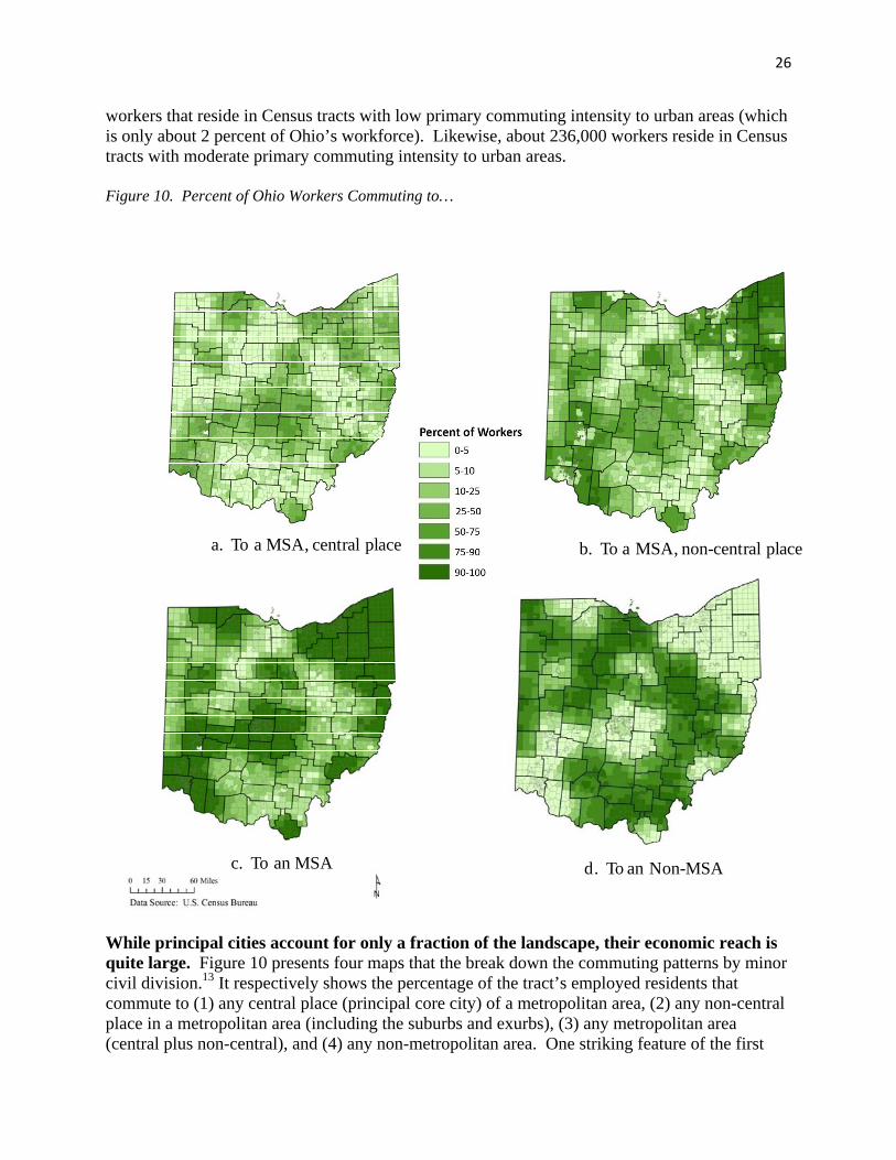
workers that reside in Census tracts with low primary commuting intensity to urban areas (which is only about 2 percent of Ohio’s workforce). Likewise, about 236,000 workers reside in Census tracts with moderate primary commuting intensity to urban areas. Figure 10. Percent of Ohio Workers Commuting to…

a. To a MSA, central place b. To a MSA, non-central place

c. To an MSA d. To an Non-MSA

While principal cities account for only a fraction of the landscape, their economic reach is quite large. Figure 10 presents four maps that the break down the commuting patterns by minor civil division.13 It respectively shows the percentage of the tract’s employed residents that commute to (1) any central place (principal core city) of a metropolitan area, (2) any non-central place in a metropolitan area (including the suburbs and exurbs), (3) any metropolitan area (central plus non-central), and (4) any non-metropolitan area. One striking feature of the first

  27

map in Figure 10a is that despite the fact that principal cities only account for a tiny share of the land mass of Ohio, their reach in terms of providing jobs to suburbanites and rural areas is far sweeping. Likewise, Figure 10b shows that the geographical reach of commuting to metropolitan jobs located outside the principal city is even larger. Reinforcing the first two maps, Figure 10c illustrates that virtually every census tract in the state has commuters working in one of the state’s 16 metropolitan areas.14 Figure 10d shows that the interdependence extends both ways with many metropolitan residents commuting to nonmetropolitan workplaces—though not as many as those who commute the other way (see footnote 12 for exact figures). 4.2.2 Case Studies of the Geographic Reach Ohio’s urban job engines. We now present three diverse commuting ‘case studies’ to illustrate why all Ohioans have a stake in the economic health of their cities. Using 2000 data, we consider Hamilton County that contains the city of Cincinnati; Allen County that contains the city of Lima; and Muskingum County contains the city of Zanesville. By describing commuting patterns surrounding Allen and Muskingum counties, we demonstrate that even small Ohio urban centers are important sources of jobs outside of their county. 4.2.2.1 Hamilton County Thirty-five percent of Hamilton County workers commute in from the countryside. Figure 11 shows the number of commuters from neighboring counties that travel into Hamilton County. There are approximately 520,000 employed workers in Hamilton County, of which, about 184,000 reside outside the county, accounting for over 35 percent of employment in Hamilton County. It is not surprising that establishments in Hamilton County employ so many workers from immediately adjacent metropolitan neighbors. For example, more than 40,000 workers employed in Hamilton County reside in both Butler and Clermont Counties. Another 15,000 of its workers reside in Campbell County (Kentucky) and another 20,000 reside in Kenton County (Kentucky). Large numbers of commuters also originate from nearby Indiana counties. Even outside of the official Cincinnati metropolitan area, there are large numbers commuting to Hamilton County. For example, nearly one thousand commuters originate in Adams County far to the southeast. Another 1,500 reside in Clinton County to the Northwest, even though Clinton County is the home of a small urban center (Wilmington). Nearly 400 Hamilton County commuters originate in Preble County even as it officially falls in the Dayton metropolitan area. In sum, an economically viable Hamilton county supports the livelihood of residents who live far away. 4.2.2.2 Allen County Even smaller Ohio metro areas draw a considerable amount if workers. Figure 12 shows the corresponding commuting flows into Allen County, home of Lima Ohio. Allen County is located in relatively less populated Northwest Ohio and is a traditional manufacturing region. Smaller commuting flows still represent a significant share of the surrounding counties workforce. For example, neighboring Van Wert, Paulding, and Putnam counties respectively

  28

Figure 11. Hamilton County In-Commute Pattern, 2000

519,981 working in the core county 183,736 or 35.3% traveling from the metro outskirtsData Source: U.S. Census Bureau

Figure 12. Allen County In-Commute Pattern, 2000

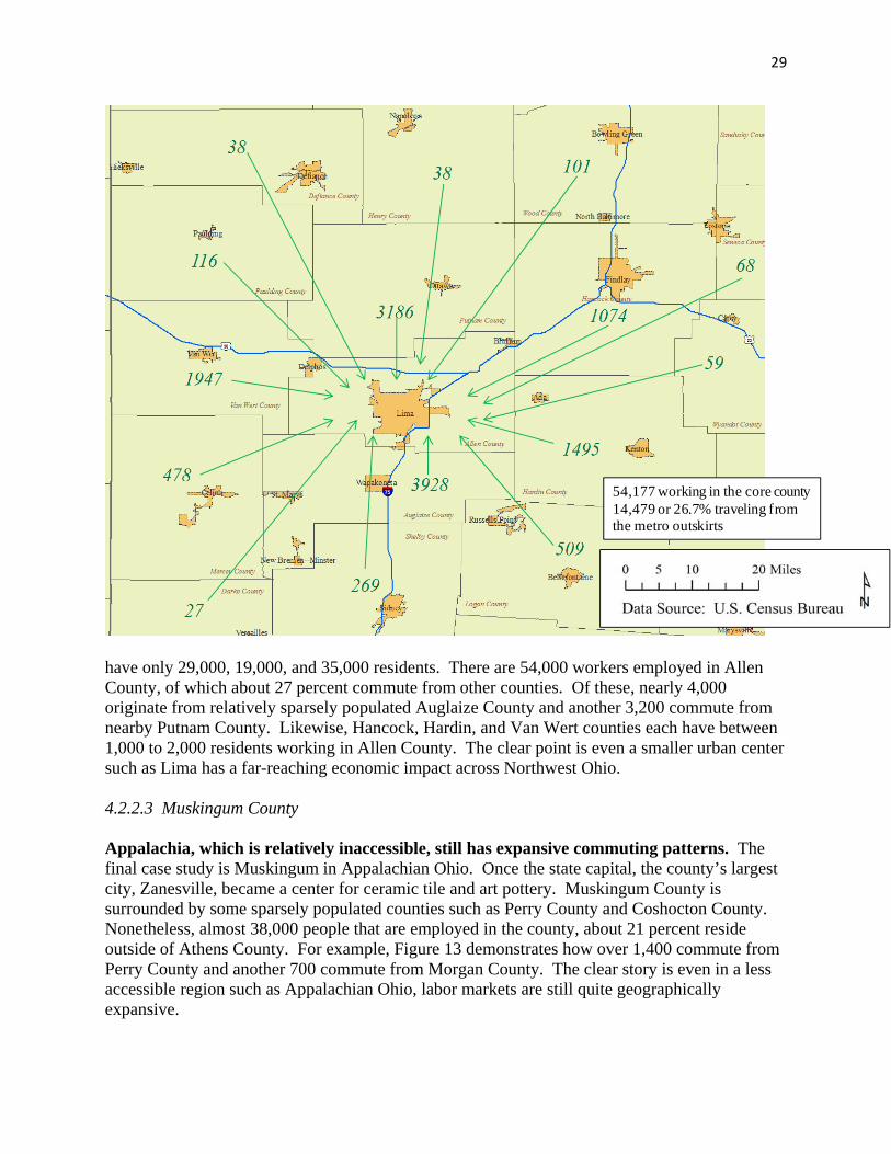
  29

54,177 working in the core county 14,479 or 26.7% traveling from the metro outskirts

have only 29,000, 19,000, and 35,000 residents. There are 54,000 workers employed in Allen County, of which about 27 percent commute from other counties. Of these, nearly 4,000 originate from relatively sparsely populated Auglaize County and another 3,200 commute from nearby Putnam County. Likewise, Hancock, Hardin, and Van Wert counties each have between 1,000 to 2,000 residents working in Allen County. The clear point is even a smaller urban center such as Lima has a far-reaching economic impact across Northwest Ohio. 4.2.2.3 Muskingum County Appalachia, which is relatively inaccessible, still has expansive commuting patterns. The final case study is Muskingum in Appalachian Ohio. Once the state capital, the county’s largest city, Zanesville, became a center for ceramic tile and art pottery. Muskingum County is surrounded by some sparsely populated counties such as Perry County and Coshocton County. Nonetheless, almost 38,000 people that are employed in the county, about 21 percent reside outside of Athens County. For example, Figure 13 demonstrates how over 1,400 commute from Perry County and another 700 commute from Morgan County. The clear story is even in a less accessible region such as Appalachian Ohio, labor markets are still quite geographically expansive.

  30

Figure 13. Muskingum County In-Commute Pattern, 2000

37,875 working in the core county 8,000 or 21.1% traveling from the metro outskirts

4.3 Linkages of Use While Ohio’s urban areas clearly draw workers into principal cities, they are also a hub for other activities such as retail and services. The retail hierarchy follows the concept of demand thresholds (Shaffer et al, 2004). Communities can be categorized by their threshold, or their population and per capita income, which then translate into demand. These community types range from those that can support minimum convenience goods and services (every day goods and services like hardware stores, drug stores, Groceries and gasoline stations) to full convenience (including such restaurants and general merchandize) to partial shopping to complete shopping and service centers that can support good and services that are not utilized on an everyday basis (highly specialized goods and services). Ohio’s major urban areas therefore are able to have the number, the diversity, and the specialization that rural areas simply cannot

  31

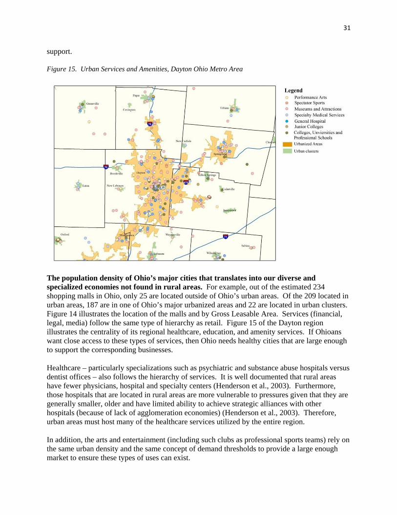
support. Figure 15. Urban Services and Amenities, Dayton Ohio Metro Area

The population density of Ohio’s major cities that translates into our diverse and specialized economies not found in rural areas. For example, out of the estimated 234 shopping malls in Ohio, only 25 are located outside of Ohio’s urban areas. Of the 209 located in urban areas, 187 are in one of Ohio’s major urbanized areas and 22 are located in urban clusters. Figure 14 illustrates the location of the malls and by Gross Leasable Area. Services (financial, legal, media) follow the same type of hierarchy as retail. Figure 15 of the Dayton region illustrates the centrality of its regional healthcare, education, and amenity services. If Ohioans want close access to these types of services, then Ohio needs healthy cities that are large enough to support the corresponding businesses.

Healthcare – particularly specializations such as psychiatric and substance abuse hospitals versus dentist offices – also follows the hierarchy of services. It is well documented that rural areas have fewer physicians, hospital and specialty centers (Henderson et al., 2003). Furthermore, those hospitals that are located in rural areas are more vulnerable to pressures given that they are generally smaller, older and have limited ability to achieve strategic alliances with other hospitals (because of lack of agglomeration economies) (Henderson et al., 2003). Therefore, urban areas must host many of the healthcare services utilized by the entire region.

In addition, the arts and entertainment (including such clubs as professional sports teams) rely on the same urban density and the same concept of demand thresholds to provide a large enough market to ensure these types of uses can exist.

  32

For reasons already discussed, the central engines of the Ohio economy are its cities. And the “brains” of the knowledge economy are the educational institutions. Ohio’s major research universities are located in urban areas and the community colleges tend to be located in urban areas as well. Many of these universities and colleges have a substantial commuter population that pulls across the region. For example, at Cleveland State University only an estimated 27.5 percent of its over 15,000 students (Cleveland State University, Institutional Research, 2007) are from the core city. The overwhelming majority are commuting from suburbs, exurban, and Ohio’s rural areas. Conversely, in addition to customer and workforce base, urban areas rely on rural for recreation, and other services. Though the focus of our discussion has been more on the dependencies of rural Ohio on urban Ohio for jobs and services, we do not want to lose sight of the urban dependencies on strong rural and exurban communities.15 In terms of economic connectedness, we have noted that many residents of the state’s principal cities and suburban areas commute to nonmetropolitan locations for employment (i.e., this commuting flow is about one-half the size of the reverse flow). Moreover, given the higher-ordered retail services in urban communities, rural shoppers form an important element of the customer market for urban businesses (not just the labor force). Rural areas have always played an important role as the primary source for food, energy and natural resources. As a reflection, there is a growing interest in exploring local food systems for economic development and community wellness. Indeed, the state of Ohio has recently formed a Figure 14. Ohio Mall Locations by Gross Leasable Area

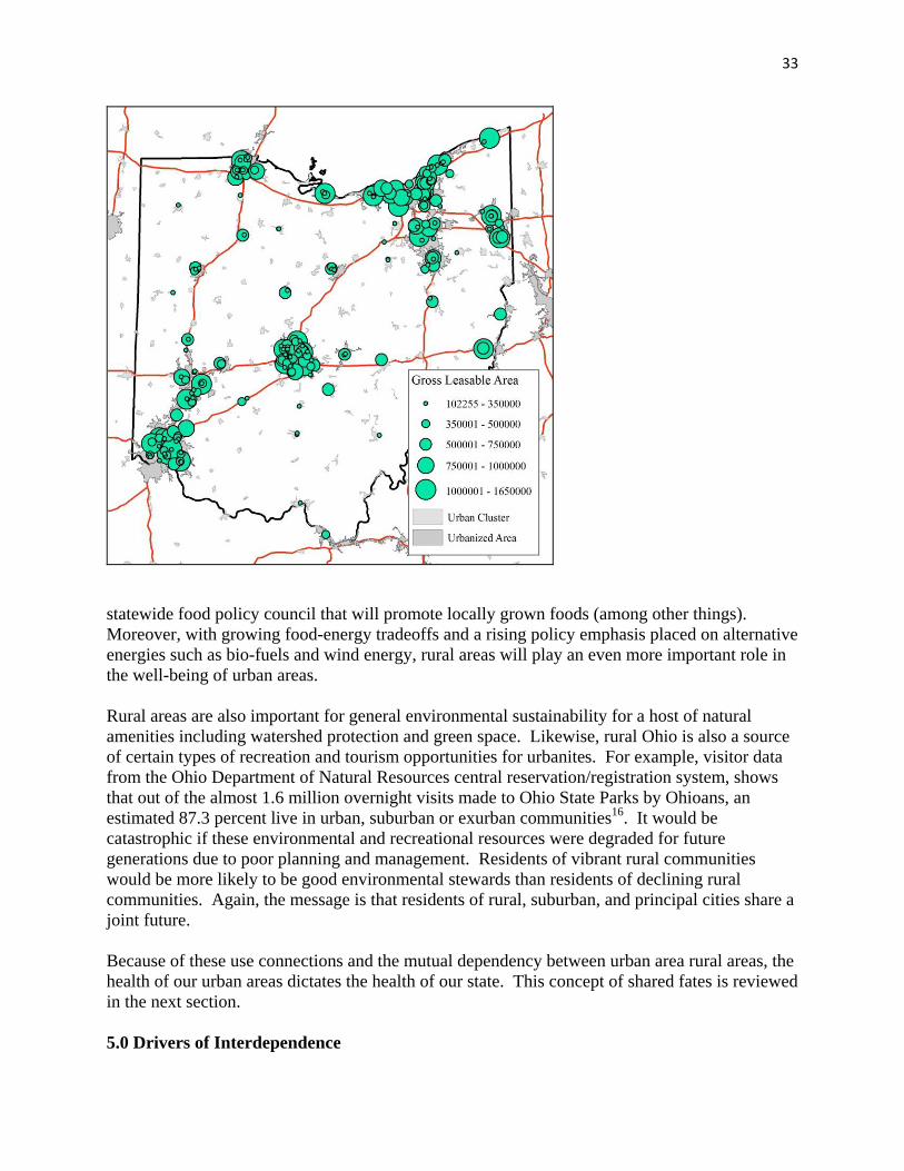
  33

statewide food policy council that will promote locally grown foods (among other things). Moreover, with growing food-energy tradeoffs and a rising policy emphasis placed on alternative energies such as bio-fuels and wind energy, rural areas will play an even more important role in the well-being of urban areas. Rural areas are also important for general environmental sustainability for a host of natural amenities including watershed protection and green space. Likewise, rural Ohio is also a source of certain types of recreation and tourism opportunities for urbanites. For example, visitor data from the Ohio Department of Natural Resources central reservation/registration system, shows that out of the almost 1.6 million overnight visits made to Ohio State Parks by Ohioans, an estimated 87.3 percent live in urban, suburban or exurban communities16. It would be catastrophic if these environmental and recreational resources were degraded for future generations due to poor planning and management. Residents of vibrant rural communities would be more likely to be good environmental stewards than residents of declining rural communities. Again, the message is that residents of rural, suburban, and principal cities share a joint future. Because of these use connections and the mutual dependency between urban area rural areas, the health of our urban areas dictates the health of our state. This concept of shared fates is reviewed in the next section. 5.0 Drivers of Interdependence

  34

People, goods, and resources move along the urban to rural spectrum. Likewise the problems and challenges that communities face are structural and systematic as well, meaning that one community’s problem in a region spills over to other communities. We now describe how spillovers and peer effects inextricably link our urban neighborhoods to the rest of their region—as well as the reverse. 5.1 Some Origins of Economic Interdependence—Peer Effects. A key factor driving the strength of the interdependence is close proximity, in particular neighborhood or peer effects (Aaronson, 2001; Partridge and Rickman, 2006; Weinberg, 2004; Weinberg et al., 2004).17 Neighborhood effects capture the simple notion that individuals look to their nearby peers as potential role models across many dimensions. Some examples include labor market attachment; engaging in non-social behavior (e.g., crime); marriage and childbearing behavior; welfare participation; and educational performance for youth. It is often argued that neighborhood and peer effects are one reason why poverty is concentrated in particular neighborhoods (including spillover effects such as low housing values or crime). Neighborhood characteristics are then transferred to the individual. Neighborhood effects could create a whole chain of causation or contagion (influence of one neighbor to another) effects where attributes from one neighborhood spillover to influence behavior and outcomes in nearby neighborhoods. This process would partially explain why inner or first-tier suburbs are increasingly taking on the attributes of the principal cities. Self interest should be enough to motivate suburban residents to want to mitigate any negative effects of concentrated poverty. For example, Partridge and Rickman (2006) find that local employment growth reduces urban poverty rates at the county level, but especially when the job growth is concentrated in central-core counties of their respective metropolitan areas. 5.2 Some Consequences of Economic Interdependence—Spillovers and Fragmented Governance Problems and challenges in one community spill over into others, even if neighborhoods or communities do not intend to mimic their neighbors. One of the key concepts in economics is the notion of externalities and spillovers. Specifically, parties outside a given economic transaction either benefit or incur costs from the transaction. The classic negative example from economics is pollution where residents near (say) a smelly factory incur costs even though they are not a buyer or seller of the product produced at the factory. Spillovers are a key underlying cause of the interdependence of rural, exurban, and suburban communities with the principal or core city. One spillover is the simple fact that since 1950, a worker’s place of residence and place of work has greatly decoupled with improvements in transportation—primarily via the automobile and highway infrastructure. The interdependencies are further deepened by the shared use and interconnectedness of the infrastructure including roadways, water and sewerage, airports, and recreation venues. The quality of the infrastructure in one part of the metropolitan area spills over and affects the quality of life and competitiveness throughout the metropolitan area.

  35

These urban, suburban, exurban and rural spillovers further deepen their “linked fates,” as outlined in a recent report by Ohio State University’s Kirwin Institute for the Study of Race and Ethnicity along with the Environmental Justice Resource Center at Clark Atlanta University for The President’s Council of Cleveland (Blackwell et al., 2007). The concept of linked fates and how inequities impair the competitive strength of an entire region can be applied across all of Ohio’s urban areas, big and small. Blackwell et al. (2007) describe how racial and social inequities across the Cleveland region has caused wasted creative capacity. Widespread educational disparities create areas that are unprepared for a knowledge-based economy. The region then lacks a large pool of highly-skilled and educated workers and this becomes a barrier for the region to attract businesses. A shared fate from negative spillovers is the result of sprawl and deconcentration. As demonstrated earlier, Ohio has not grown so much in absolute population, but population has deconcentrated across the state. This deconcentration is followed by retail and service providers who often employ more unskilled workers. This results in a spatial mismatch, when lower income residents suffer since they live in areas of concentrated poverty far from jobs. Public transportation networks are not designed for this type of settlement pattern, which would often require transporting less-skilled workers from the central core to the expanding outer suburbs. Therefore, it is more difficult for workers who rely on public transportation to get these types of jobs. This negatively affects the entire economy of the region, further illustrating why regions need more collaborative engagement (Moore, 2008). Ohio’s regions filled with “fragmented economic voices” too often pit one small box jurisdiction against another small box jurisdiction in a zero (or negative)-sum game of economic development or related competition.

Side Box 2. Case examples of Linkages of Fate As we described in Sections 4 and 5, whether the economic history or outlook of an urban seems promising or hopeless, it translates into the entire region’s history and outlook. For example, the stories of Cleveland, Minneapolis and Seattle could not be more different, yet they all demonstrate the interconnectedness of the urban core to the rest of the region. Research has shown that regional disparities depress the productivity, earnings, and overall quality of life for everyone across the metropolitan area (Blackwell et al., 2007). Cleveland’s economic story is well known and fits with other tales of Rust Best cities. With its reliance on heavy manufacturing, and the lagging growth of 21st century sectors, the city has hit hard times. In the 1930s, Cleveland was the 3rd largest city in the US. But since the 1950s, the population of the city declined. While regional population barely grew, the population decentralized throughout the region. Cleveland suffers from one of the largest vacant property problems in the country. Industry and jobs decentralized as well. Less than one-third of the region’s workers are employed in the city (The Brookings Institution, 2003). Cleveland’s population is older with relatively fewer young people, and its workforce tends to be less educated. The city’s poverty rate is among the highest for any big city in the nation. Like the rest of Ohio, Cleveland suffers from fragmented governments, spurring recent efforts to build collaboration in Northeast Ohio. For the Midwest, Minneapolis-St. Paul is a bright light in the Midwest region. While decentralizing like Cleveland, Minneapolis-St. Paul is balancing its growth with vibrant development in the downtown. Minneapolis-St. Paul’s gross metropolitan product is 14th in the nation, right after Seattle (Global Insight, 2006), while per capita income ranked 7th (U.S. Bureau of Economic Analysis, www.bea.gov). Conversely, despite its storied history, Cleveland ranks 25th in

gross metropolitan product. Minneapolis-St. Paul is also buoyed by its vibrant educational sector that includes the University of Minnesota’s main campus and a long history of technology-related firms. Like Seattle, Minneapolis-St. Paul has been able to reinvent itself over time as the economy evolves: from agriculture center and food processing capital to latter 20th Century high-technology leader such as in mainframe computers to 21st Century leader in emerging technologies such as in medical sciences. But what makes the Minneapolis-St. Paul metro region really stand out is its 40-plus years of regional policy and planning to help coordinate its over 240 local jurisdictions (Metropolitan Council, 2008). In particular, the region’s revenue sharing policy is still viewed as one of the most innovative in the country. The seven core metropolitan counties place 40% of the growth in the commercial and industrial tax base into a region-wide pool. The funds in this pool are then redistributed to communities based on their population and fiscal capacity. The intention is to address the fiscal disparities between the core city and its suburbs and exurbs. Thus, the entire region shares in the benefits of growth, creating a better cooperative environment. In 2007, these funds reached $303 million (Metropolitan Council, 2008). Seattle is considered to be a healthy metropolitan region. A diverse economy that relies on aerospace and software, as well as emerging strengths in biotech and electronic commerce have created a strong metro economy. Research has shown that these high tech jobs have clustered in Seattle’s urban core, which in turn supports a healthy downtown retail sector in conjunction with traditional office functions (Sommers et al., 2000). Unlike Cleveland, the city is able to hang on to half the jobs in the region. Further supporting its economic health, the Seattle metro area is marked by high levels of education, income, and population growth. Figures 16-19 demonstrate indicators of overall metro health: population growth,

  36

In fact, the state is at particular risk for fragmented governance. With barely 40,000 square miles, it has nearly 3,800 local governmental jurisdictions of various types including 939 municipalities (cities and villages) and 1,308 townships (Vitale, 2007). The resulting negative spillovers across these small boxes can result in inefficient provision of government services and sub-optimal provision of infrastructure that lacks a broader regional focus. Transportation issues often have implications that extend from outside the boundaries of a suburban municipality or a township. Planning and zoning likewise has related regional spillovers. For example, the loss of green space on the urban fringe affects an entire region’s quality of life. Similarly, environmental issues such as the watershed protection or air pollution are not limited to single municipalities. Fragmented governance is linked to bad outcomes. Fragmented local governance produces a negative externality because each individual jurisdiction does not fully consider how their actions affect other jurisdictions. The most egregious example is tax poaching where one jurisdiction lures a business from a nearby jurisdiction through offering tax breaks. No new wealth is created by tax poaching, but both communities have directly or indirectly lost some of their tax base. Another example is when a community chooses not to build a widely desired piece of infrastructure (say a road or a cultural venue) because many of the people who would benefit from the project live outside the jurisdiction and would not be required help pay for the project. Another example of a common spillover or externality is when one jurisdiction captures an economic development that provides it significant tax revenues (say a new factory), but neighboring jurisdictions are forced to pay significant costs without sufficient new revenues—e.g., new residents move into these other jurisdictions forcing the construction of new infrastructure. Besides not considering the spillovers of their decisions, such fragmented governments can lack accountability. Clearly, when there is a situation where “everyone is in charge,” then the reality is “no one is in charge” and local constituents won’t know who to blame when things inevitably go wrong. Moreover, the local region speaks with a fractured voice and is less able to lobby the business community or the federal and state governments. Besides increasing negative spillovers, fragmented governments are usually not at the efficient scale or size to provide government services. First, each government jurisdiction needs an administrative structure to provide services. The size of this administrative structure usually does not need to grow at the same rate as the population being served. Second, many services such as fire protection, emergency management, and police services have a range in which average costs per-capita decline as serviced population increases. Joint purchasing arrangements can achieve quantity discounts. Throughout Ohio, there are pushes for local governments to achieve many of these cost savings and any reductions in the costs of providing services will help enhance the competitiveness of the state’s businesses. A recent example includes Hamilton County’s Government Cooperation and Efficiency Project to help its over 50 local governments collaborate and share services to increase efficiencies, improve service delivery, and minimize costs (http://www.hamiltoncountyohio.gov/hcrpc/partner/gcep/).

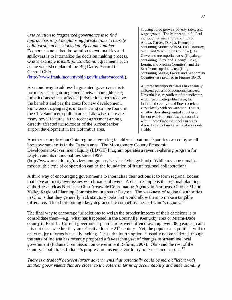
  37

One solution to fragmented governance is to find approaches to get neighboring jurisdictions to closely collaborate on decisions that affect one another. Economists note that the solution to externalities and spillovers is to internalize the decision making process. One is example is multi-jurisdictional agreements such as the watershed plan of the Big Darby Accord in Central Ohio (http://www.franklincountyohio.gov/bigdarbyaccord/). A second way to address fragmented governance is to form tax-sharing arrangements between neighboring jurisdictions so that affected jurisdictions both receive the benefits and pay the costs for new development. Some encouraging signs of tax sharing can be found in the Cleveland metropolitan area. Likewise, there are many novel features in the recent agreement among directly affected jurisdictions of the Rickenbacker airport development in the Columbus area. Another example of an Ohio region attempting to address taxation disparities caused by small box governments is in the Dayton area. The Montgomery County Economic Development/Government Equity (ED/GE) Program operates a revenue-sharing program for Dayton and its municipalities since 1989 (http://www.mcohio.org/revize/montgomery/services/ed/edge.html). While revenue remains modest, this type of cooperation can be the foundation of future regional collaborations. A third way of encouraging governments to internalize their actions is to form regional bodies that have authority over issues with broad spillovers. A clear example is the regional planning authorities such as Northeast Ohio Areawide Coordinating Agency in Northeast Ohio or Miami Valley Regional Planning Commission in greater Dayton. The weakness of regional authorities in Ohio is that they generally lack statutory tools that would allow them to make a tangible difference. This shortcoming likely degrades the competitiveness of Ohio’s regions.18 The final way to encourage jurisdictions to weigh the broader impacts of their decisions is to consolidate them—e.g., what has happened in the Louisville, Kentucky area or Miami-Dade county in Florida. Current government jurisdictions were often drawn up over 100 years ago and it is not clear whether they are effective for the 21st century. Yet, the popular and political will to enact major reforms is usually lacking. Thus, the fourth option is usually not considered, though the state of Indiana has recently proposed a far-reaching set of changes to streamline local government (Indiana Commission on Government Reform, 2007). Ohio and the rest of the country should track Indiana’s progress in this endeavor to try to learn some lessons.19 There is a tradeoff between larger governments that potentially could be more efficient with smaller governments that are closer to the voters in terms of accountability and understanding

housing value growth, poverty rates, and wage growth. The Minneapolis-St. Paul metropolitan area (core counties of Anoka, Carver, Dakota, Hennepin-containing Minneapolis-St. Paul, Ramsey, Scott, and Washington Counties), the Cleveland metropolitan area (Cuyahoga-containing Cleveland, Geauga, Lake, Lorain, and Medina Counties), and the Seattle metropolitan area (King-containing Seattle, Pierce, and Snohomish Counties) are profiled in Figures 16-19. All three metropolitan areas have widely different patterns of economic success. Nevertheless, regardless of the indicator, within each metropolitan area, the individual county trend lines correlate very closely with one another. That is, whether describing central counties or far-out exurban counties, the counties within these three metropolitan areas share the same fate in terms of economic health.

  38

the voters’ wishes. It is easy to argue that fragmented governments are draining the fiscal resources of Ohio without providing corresponding levels of services. Yet, we do caution that this does not mean that having a healthy variety of local jurisdictions is always harmful. Specific, one positive feature of diverse local governments is that people can “vote with their feet” and choose to reside in the jurisdiction with the level of taxes and services that fit their preferences (Tiebout, 1956). For example, a voter may want to live in a jurisdiction with high taxes, with good public schools, and high-quality services. Yet, another voter may want to live in a jurisdiction with low taxes and fewer public services. Finally, smaller governments may be closer to the people, assuming voters understand the array of jurisdictions and their responsibilities. In sum, competitive regions avoid fragmented governance, while still providing adequate choice for their residents. Ohioans criss-cross the landscape whether it is to generate income, utilize educational services, healthcare, airports, or recreation. For reasons such as agglomeration economies and demand thresholds, Ohio’s urban areas host many services and amenities. Likewise, because of the landscape rural areas contain features that generate a rural economy and rural amenities as well. As demonstrated, the rural/exurban/suburban/core interdependencies exist, but they are complex. These linkages exist and are complex not only for the Cleveland, Columbus and Cincinnati regions, but for our smaller regions like Athens, Canton and Marietta. Because of reasons such as peer effects and spillovers, these linkages link livelihoods, use, and in the end, the fate of Ohio. To bring in lessons from other states, Side Box 2 compares how Cleveland is faring compared to what are thought to be healthy regions—Seattle and Minneapolis-St. Paul. 5.3 Quantifying Spillovers and Peer Effects

We now provide evidence of the interdependence of communities. Specifically, we use the Moran I statistic that allows us to test the strength of relationships between nearby places and the overall statistical significance of these relationships (Anselin et al., 2006).20 When examining the results (which range between 0 and 1), a greater positive value suggests that county poverty rates are clustered, which is consistent with spillovers across places.

Across Ohio, poverty rates and median housing values in one county are related to nearby counties. We first considered these types of interdependencies across all Ohio counties for two key indicators: median housing values and poverty rates.21 The Moran I scores for the poverty rate equaled 0.5522, implying that neighboring counties had similar poverty rates—i.e., counties with high poverty rates tended to be located near counties with high poverty rates—and vice versa. These clusters of high and low poverty are suggestive of common underlying factors that affect poverty rates in multiple counties. Some potential reasons could include peer effects that spread across broader regions (see section 5.1) or labor market factors that are spread due to commuting patterns (see section 4.2). For example, a weak labor market in one part of a metropolitan area affects workers throughout the metro area due to commuting.

We also find a relative high Moran I statistic for median housing values (Moran I= 0.79). This implies that counties with high median housing values are located near counties with high median housing values (and vice versa). Again, such a spatial pattern of housing values illustrates how problems in one county can spread into neighboring counties. That is, residents of a county cannot simply wall themselves off from poorly performing neighbors. They too

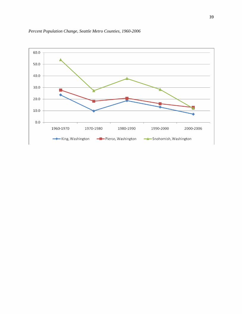
  39

Percent Population Change, Seattle Metro Counties, 1960-2006

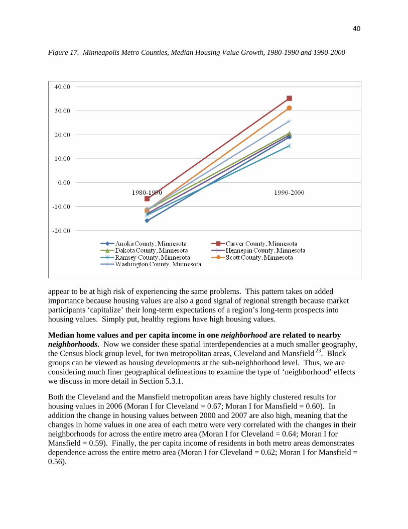
  40

Figure 17. Minneapolis Metro Counties, Median Housing Value Growth, 1980-1990 and 1990-2000

appear to be at high risk of experiencing the same problems. This pattern takes on added importance because housing values are also a good signal of regional strength because market participants ‘capitalize’ their long-term expectations of a region’s long-term prospects into housing values. Simply put, healthy regions have high housing values.

Median home values and per capita income in one neighborhood are related to nearby neighborhoods. Now we consider these spatial interdependencies at a much smaller geography, the Census block group level, for two metropolitan areas, Cleveland and Mansfield 23. Block groups can be viewed as housing developments at the sub-neighborhood level. Thus, we are considering much finer geographical delineations to examine the type of ‘neighborhood’ effects we discuss in more detail in Section 5.3.1.

Both the Cleveland and the Mansfield metropolitan areas have highly clustered results for housing values in 2006 (Moran I for Cleveland = 0.67; Moran I for Mansfield = 0.60). In addition the change in housing values between 2000 and 2007 are also high, meaning that the changes in home values in one area of each metro were very correlated with the changes in their neighborhoods for across the entire metro area (Moran I for Cleveland = 0.64; Moran I for Mansfield = 0.59). Finally, the per capita income of residents in both metro areas demonstrates dependence across the entire metro area (Moran I for Cleveland = 0.62; Moran I for Mansfield = 0.56).

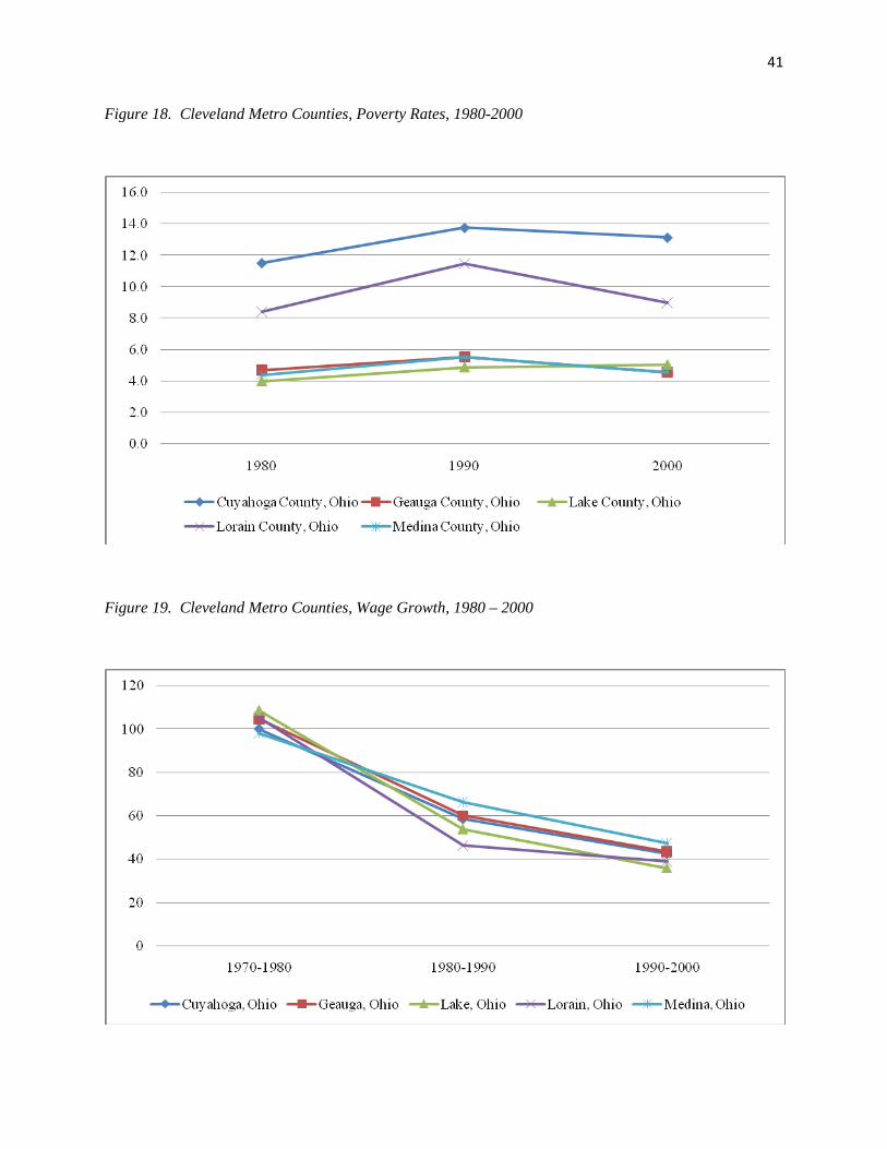
  41

Figure 18. Cleveland Metro Counties, Poverty Rates, 1980-2000

Figure 19. Cleveland Metro Counties, Wage Growth, 1980 – 2000

  42

What is most telling is that despite the fact that Mansfield and Cleveland are seemingly different types of metropolitan areas, by size, by population, by social and economic structures, the results tell a very strong story of neighborhood interdependence across the urban/suburban/exurban/rural landscape.

6.0 Summary and Recommendations. Ohio’s economy has been one of the weakest performing since the late 1960s, even lagging its Great Lakes state neighbors. This weak performance continues in recent years. The long-term nature of Ohio’s economic woes illustrates that popular explanations for these problems such as international trade and declining manufacturing are inadequate in explaining Ohio’s performance. Instead, the problems point to systemic problems that will not be solved by minor tweaks in existing programs or reliance on the latest fads in economic development. In assessing Ohio’s economy, this report described the strong interdependencies that link our central cities, suburbs, exurbs, and rural communities together. These interdependencies go both ways, though we primarily focused on how all Ohioans rely on the health of our cities and metropolitan areas for economic prosperity and quality of life. What we showed is that the state’s citizens rely on urban centers as a source of jobs, higher-ordered retail establishments, and a source of important shared goods such as for healthcare and venues for culture/entertainment. Of course, this does not belittle the urban interdependencies on rural Ohio for a clean environment, food, natural resources, recreation, and workforce, but this was not the topic of this report. This report also showed that it is almost impossible for communities or wealthy enclaves to wall themselves from the broader trends experienced in Ohio’s small and large metropolitan centers. Whether considering home values, poverty rates, population change, or commuting patterns, there is simply too many spillovers for one community to ignore the economic and social trends in its neighboring communities. Moreover, we illustrated how economic linkages from urban areas extend far out into exurbia and into more distant rural communities as well. These interdependencies illustrate that shared linkages that exist across the entire state. Ohio’s city-centered regions don’t just compete with each other, but they compete with metropolitan regions throughout the world. If Ohio’s regions are slightly less competitive than their global rivals, workers, entrepreneurs, and financial capital will flow elsewhere. The goal is then for Ohio’s regions to be more competitive for both workers and investors alike. This report also discussed the need to make Ohio’s city-centered regions perform more effectively. Foremost, the large geographical interdependence indicates the gains from regionalization of economic development, planning, and service provision. The timing may be right as the Ohio legislature is considering a study commission to examine how to make the state’s local governments more efficient to compete in the 21st century (HB521). Though change may be years away, there is much to gain if such a process was successful in streamlining local government to help make the state more globally competitive. In particular, policymakers and potential study commissions should consider ways to: 1. Have local governments more effectively share revenue so that entire regions receive the

  43

benefits and pay the costs of development. Too often, one municipality is able to take the benefits of development, while pushing the costs onto its neighbors. Revenue sharing would also mitigate the incentives for destructive tax poaching as the tax revenues would then be dispersed across the broader region. To be truly effective, tax sharing cannot just be limited to a handful of interested municipalities, but should include all jurisdictions in multiple-county regions. The Metropolitan Council surrounding Minneapolis-St. Paul would be one model. 2. Streamline local governments and create more effective regional planning & economic development authorities. Currently, there are so many layers of government that lines of accountability and transparency are blurred. Likewise, economic development initiatives often include an inordinate numbers of local governments that delay and complicate decision making. State statutes should be changed to provide regional organizations more effective taxation and planning and implementation tools to become truly effective. Regional organizations can then weigh economic development for urban and rural residents with coherent planning at the rural-urban interface. Similarly, the state should explore ways to eliminate unnecessary local governments that no longer make sense in the 21st century, though we acknowledge that considerable study and public education would be necessary to produce solutions acceptable to most Ohioans. Section 5.2 also provided other common-sense ways to increase regional collaboration including strategic use of multi-jurisdictional agreements in planning and purchasing. 3. More effective state revenue sharing with Ohio’s regions after they have undergone needed reforms. A key goal of state revenue sharing would be to help reduce local taxes, especially earnings taxes that help make the state’s regions less competitive in attracting entrepreneurs and knowledge workers. In other words, state funding could be the “grease” that smoothes the formation of true regions. Yet, despite the gains from regional approaches and tax sharing, local governments too often continue with the status quo. Thus, to further incentivize local governments, state economic development funding should be directed to areas that have adopted coherent regional plans. 4. Provide state infrastructure funding on a regional basis. Infrastructure funds should be prioritized to projects that make the entire region more competitive, not just isolated communities. Again, regional plans should be a requirement for state infrastructure funding. What we are proposing is linking urbanites, suburbanites, with their rural cousins in a new rural-urban compact for a shared prosperity. Needless to say, many of these proposals would be controversial. However, it is virtually impossible to imagine a scenario in which Ohio is able to reverse its economic woes without making changes that would be viewed as controversial, or even painful in the short-term. Yet, we believe that successful change will require recognition that all Ohioans share a common future and recognizing that managing these interdependencies will promote a better future.

  44

About the Authors Mark Partridge is the C. William Swank Chair of Rural-Urban Policy at The Ohio State University and a professor in the Agricultural, Environment, and Development Economics Department. Prior to that, he was the Canada Research Chair in the New Rural Economy at the University of Saskatchewan, where he is an adjunct professor. Professor Partridge has published over 75 academic and scholarly papers and his work has been ranked among the top-1000 economists in the world. He co-authored a book entitled The Geography of American Poverty: Is there a Role for Place-Based Policy? published by the W.E. Upjohn Institute. He is currently the lead investigator on an Infrastructure Canada grant to examine rural-urban interactions and for an Appalachian Regional Commission project evaluating measures of community distress. Partridge’s current research interests include investigating rural-urban interdependence, why some communities grow faster than others, and innovations in regional policy and governance. Professor Partridge served as President of the Southern Regional Science Association. He is currently the co-editor of the Journal of Regional Science and is on the executive council of the Regional Science Association International. Partridge has consulted with various governments in the U.S. and Canada and has testified to the U.S. Congress and the Canadian Parliament on regional issues. Partridge received his Ph.D. in economics from the University of Illinois. Jill Clark is the director for The Center for Farmland Policy Innovation, housed in the Department of Agricultural, Environmental and Development Economics at the Ohio State University. The center is designed to match local farmland protection goals with needed resources. Through these local-state partnerships, the center provides model farmland protection strategies for Ohio communities and other interested partners. Jill Clark also manages the Exurban Change Project. The goal of the Exurban Change Project is to analyze patterns and trends in Ohio's rural-urban interface areas. Prior to joining the Department in November 2002, Clark managed American Farmland Trust's Ohio Field Office for three years. American Farmland Trust is a national nonprofit organization dedicated to farmland protection. She also spent three years conducting research at the University of Wisconsin's Program on Agricultural Technology Studies and the Wisconsin Land Use Research Program. Jill has a M.S. in land resources from the University of Wisconsin and is a Ph.D. candidate in Ohio State University’s Department of Geography.  

  45

                                                            

1Low density development is defined as areas with development densities of 5 to 40 acres per household. Irwin and Reece (2002) provide a nice background for defining exurban Ohio. 2Ohio and these four states form the Great Lakes region (or East North Central Region) in U.S. Census Bureau and U.S. Bureau of Economic Analysis reporting. 3Source for the 1970-2005 total employment, U.S. Bureau of Economic Analysis, REIS data available at www.bea.gov (downloaded April 20, 2008). Source for the nonfarm employment growth since 2006, U.S. Bureau of Economic Statistics, Current Employment Statistics available at: http://www.bls.gov/sae/home.htm (downloaded on April 20, 2008). 4The employment data by sector is drawn from the U.S. Bureau of Economic Analysis REIS data, which counts the number of jobs. For example, if a person works part-time in two jobs, REIS counts this as two jobs (not one worker). The advantage of this measure is that it captures all forms of employment, but it does not weight for full versus part-time employment. 5Source, U.S. Bureau of Economic Analysis, REIS data available at www.bea.gov (downloaded April 20, 2008). The auto industry is defined as NAICS code 518—i.e., motor vehicles, bodies and trailers, and parts manufacturing. 6The reasons for Ohio’s relative decline are many including the following. First, amenity driven migration greatly favored the Sunbelt and the west at the expense of Northern States. Second, Ohio’s manufacturers began to lose a great competitive edge in the 1950s as larger shares of Americans moved west and to the Sunbelt. Ohio was no longer proximate to such a large share of North American population. This was confounded by rapid productivity growth in manufacturing—though good for the viability of the firms—it increasingly met fewer workers were producing more output. That is, Ohio’s manufacturers are productive, but as a result, they employ fewer people than in the state’s heyday. While globalization has increased competitive pressures, the real problem with the decline of manufacturing is that the state has been slow to adopt alternative base sectors. Third, Ohio’s relatively low educational attainment has placed the state at a competitive disadvantage in the emerging knowledge economy. Fourth, many have argued that Ohio’s struggles have been exacerbated by a rising relative tax burden. In 1977, Ohio’s state and local tax burden ranked 48th among U.S. states, remarkably rising to 5th highest by 2007 (Tax Foundation, 2007). Fifth, as described in Section 5, Ohio has many local governments that may not be collaborating to achieve regional prosperity. 7For example, Cleveland ranked 47th out of 49 in terms of 2000-2005 population growth for U.S. metropolitan areas with more than 1 million population in 2000. Among the nation’s 64 metropolitan areas with between 400,000 and 1 million population in 2000, Ohio’s five medium-sized metropolitan areas ranked between 57th and 63rd in terms of population growth. Finally, among the 249 U.S. metropolitan areas with less than 400,000 population in 2000, Ohio’s eight representatives ranked between 216 and 248. 8 Source: U.S. Census Bureau, www.census.gov; U.S. Census Bureau, Technical Documentation for SF1, issued July 2007, available at: www.census.gov/prod/cen2000/doc/sf1.pdf.   

9 More discussion of other measures of urban-rural continuums can be found in Isserman (2005), though his proposed measures are generally based on land-use.  

10Berube et al. (2006) describe the rapid growth of exurbia across the nation. One of their main conclusions about exurbia across the U.S. also applies to Ohio: exurbia is very diverse and hard to characterize. 11For purposes of discussion, we combine exurbs and suburbs together in section 4.1 as “suburbs.” 12 Classifying exurban residents in metropolitan or nonmetropolitan areas, about 91,000 metropolitan Ohio residents work in nonmetropolitan Ohio while about 183,000 nonmetropolitan Ohioans work in metropolitan Ohio (not shown in this data). 13A minor civil division is a county subdivision type of governmental unit that is the primary governmental or administrative division of a county or statistically equivalent entity (Census). 14The values in reported Figure 10c is derived by summing the commuting shares shown Figures 10a and 10b. 

  46

                                                                                                                                                                                                

15See Dabson (2007) for more discussion of this topic. 16 The visitor data was provided by Patti Barnett, Marketing Section Manager, Ohio Department of Natural Resources, Division of Parks & Recreation. The data, aggregated by zip code, provides the number of visitors from the central reservation/registration system and represents visitors for all state-operated overnight facilities. The data is generated from both the park locations and reservations made through the call center and the internet. 17The validity of neighborhood effects is not universally accepted. For example, Page and Solon (2003) contend that neighborhood effects relate more to family effects and effects related to growing up in broader urban areas than what is happening in more proximate neighborhoods. 18Vey (2007) also describes other ways to enhance regional coordination and collaboration. 19Illustrating the growing pressures to rationalize Ohio’s local governments, HB 521 was introduced in the Ohio House in Spring 2008 to create a study commission similar to Indiana’s. The purpose would be for this commission to recommend changes (if any) to Ohio’s local governance structure (Siegal, 2008). 20 The Moran I is based on the correlation of a particular area’s outcome with the average outcome of surrounding areas. For example, if the Moran I statistic for an area’s poverty rate equals 1.0, this would imply that all counties are perfectly related to their neighboring county poverty rates (clustered pattern). Conversely, a Moran I statistic equal to -1.0 would imply that all county’s poverty rates are exactly inversely related to neighboring county poverty rates (a checkered pattern). Finally, a value of 0 would imply no spatial relationship between the county’s poverty rate and its neighboring county poverty rates (random pattern).  21 The neighboring county averages were based on the weighted average across all the other 87 counties in the state, where the weights are the inverse distance (1/d) between the counties. Thus, closer counties are weighted much more than more distant counties in this calculation. 22 To test the significance of the results, randomization was used which compares the actual distribution of values to a random simulated distribution of values. This is the recommended approach (Anselin, 1995). The number of permutations the actual data was compared to was 999 permutations. For each Moran I result reported, the significance level is p = 0.001. 23 Defined by the U.S. Census Bureau, block groups are a statistical subdivision of a census tract and are composed of contiguous census blocks, which are the smallest level of geography in the census and are used for 100% data tabulations. For the block groups, nearest neighbors were considered in determining the Moran I. References Aaronson, Daniel. 2001. “Neighborhood Dynamics,” Journal of Urban Economics 49: 1-31.

Anselin, Luc. 1995. “Local indicators of spatial association-LISA.” Geographical Analysis 27(2): 9-115. Anselin, Luc, Ibnu Syabri, and Youngihn Kho. 2006 “GeoDa: An Introduction to Spatial Data Analysis” Geographical Analysis 38 (1): 5–22.

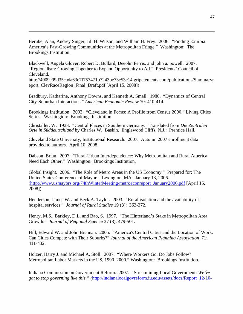
  47

                                                                                                                                                                                                

Berube, Alan, Audrey Singer, Jill H. Wilson, and William H. Frey. 2006. “Finding Exurbia: America’s Fast-Growing Communities at the Metropolitan Fringe.” Washington: The Brookings Institution. Blackwell, Angela Glover, Robert D. Bullard, Deeohn Ferris, and john a. powell. 2007. “Regionalism: Growing Together to Expand Opportunity to All.” Presidents’ Council of Cleveland. http://4909e99d35cada63e7f757471b7243be73e53e14.gripelements.com/publications/Summaryreport_ClevRaceRegion_Final_Draft.pdf [April 15, 2008]) Bradbury, Katharine, Anthony Downs, and Kenneth A. Small. 1980. “Dynamics of Central City-Suburban Interactions.” American Economic Review 70: 410-414. Brookings Institution. 2003. “Cleveland in Focus: A Profile from Census 2000.” Living Cities Series. Washington: Brookings Institution.

Christaller, W. 1933. “Central Places in Southern Germany.” Translated from Die Zentralen Orte in Süddeutschland by Charles W. Baskin. Englewood Cliffs, N.J.: Prentice Hall.

Cleveland State University, Institutional Research. 2007. Autumn 2007 enrollment data provided to authors. April 10, 2008. Dabson, Brian. 2007. “Rural-Urban Interdependence: Why Metropolitan and Rural America Need Each Other.” Washington: Brookings Institution. Global Insight. 2006. “The Role of Metro Areas in the US Economy.” Prepared for: The United States Conference of Mayors. Lexington, MA. January 13, 2006. (http://www.usmayors.org/74thWinterMeeting/metroeconreport_January2006.pdf [April 15, 2008]). Henderson, James W. and Beck A. Taylor. 2003. “Rural isolation and the availability of hospital services.” Journal of Rural Studies 19 (3): 363-372. Henry, M.S., Barkley, D.L. and Bao, S. 1997. “The Hinterland’s Stake in Metropolitan Area Growth.” Journal of Regional Science 37 (3): 479-501. Hill, Edward W. and John Brennan. 2005. “America's Central Cities and the Location of Work: Can Cities Compete with Their Suburbs?” Journal of the American Planning Association 71: 411-432. Holzer, Harry J. and Michael A. Stoll. 2007. “Where Workers Go, Do Jobs Follow? Metropolitan Labor Markets in the US, 1990–2000.” Washington: Brookings Institution. Indiana Commission on Government Reform. 2007. “Streamlining Local Government: We’ve got to stop governing like this.” (http://indianalocalgovreform.iu.edu/assets/docs/Report_12-10-

  48

                                                                                                                                                                                                

07.pdf [April 1, 2008]). Irwin, Elena G. and Jason Reece. 2002. “Urbanization trends in Ohio: Tracking Ohio's urban growth and land use change.” The Exurban Change Project Report Number EX-4. Columbus, Ohio: Ohio State University’s Exurban Change Project (http://exurban.osu.edu/EX4.htm [April 25, 2008]). Isserman, Andy M. 2005. “In the National Interest: Defining Rural and Urban Correctly in Research and Public Policy.” International Regional Science Review. 28: 465-499. Kahn, R., P.F. Orazem, and D.M. Otto. 2001. “Deriving Empirical Definitions of Spatial Labor Markets: The Roles of Competing versus Complementary Growth.” Journal of Regional Science 41 (4): 735-56. Kurban, Hydar and Joseph Persky. 2007. “Do Metropolitan Areas With Rich Central Cities Experience Less Sprawl?” Economic Development Quarterly 21: 179-184. Leichenko, Robin M. 2001. “Growth and Change in U.S. Cities and Suburbs.” Growth and Change 32: 326-354. Metropolitan Council. 2008. “A bold experiment: the Metropolitan Council at 40.” (http://www.metrocouncil.org/about/metcouncilhistory.pdf [May 9, 2008]). Moore, Charles. 2008. “Combat Poverty with a Regional Approach.” Albany Times Union. (March 9). (www.timesunion.com [March 25, 2008]). Page, Marianne E., and Gary Solon. 2003. “Correlations between Brothers and Neighboring Boys in Their Adult Earnings: The Importance of Being Urban.” Journal of Labor Economics 21(4): 831-855. Partridge, Mark. D. and Dan S. Rickman. 2006. The Geography of American Poverty: Is There a Role for Place Based Policy? Kalamazoo, MI: W.E. Upjohn Employment Institute.

Partridge, Mark D., Ray Bollman, M. Rose Olfert and Alessandro Alasia. 2007a. “Riding the Wave of Urban Growth in the Countryside: Spread, Backwash, or Stagnation.” Land Economics 83(2): 128-152. Partridge, Mark, Jill Clark, and Ayesha Enver. 2007b. “Growth and Change: Employment Growth, Future Prospects, and Change at the Ohio Rural-Urban Interface.” The Exurban Change Project and Swank Program in Rural-Urban Policy Summary Report. (www.aede.osu.edu/programs/Swank [April 23, 2008]). Partridge, Mark D., Dan S. Rickman, Kamar Ali and M. Rose Olfert. 2008a. “Agglomeration Spillovers and Wage and Housing Cost Gradients across the Urban Hierarchy.” Swank Program in Rural-Urban Policy (www.aede.osu.edu/programs/Swank [March 13, 2008]).

  49

                                                                                                                                                                                                

_____. 2008b. “Employment Growth in the American Urban Hierarchy: Long Live Distance.” Berkeley Journal of Macroeconomics—Contributions. 8 (1) (http://www.bepress.com/bejm/vol8/iss1/art10 [March 13, 2008]).

Poppert, Patrick E. and Henry W. Herzog Jr. 2003. “Force Reduction, Base Closure, and the Indirect Effects of Military Installations on Local Employment Growth.” Journal of Regional Science (43): 459-481. Puentes, Robert and David Warren. 2006. “One-Fifth of America: A Comprehensive Guide to America’s First Suburbs.” Washington: Brookings Institution. Rappaport, Jordan. 2005. “The Shared Fortunes of Cities and Suburbs.” Economic Review Federal Reserve Bank of Kansas City, Third Quarter, 33-60. Shaffer, Ron, Steve Deller and Dave Marcouiller. 2004. Community Economics: Linking Theory and Practice. Ames, Iowa: Blackwell Publishing Sharp, J. S., and Jill K. Clark. 2008. "Communities between the Country and the Concrete: Rediscovering the Rural-Urban Fringe." City & Community 7 (1): March: 61-79. Siegal, Jim. 2008. “Government May Go on a Diet.” Columbus Dispatch. April 7, p. B1. Sommers, Paul, Daniel Carlson, Michael Stranger, Saiju Xue and Mika Miyasato. 2000. “The New Economy in Metropolitan Seattle.” Washington: Brookings Institution. Tax Foundation. 2007. “State and Local Tax Burdens by State, 1970-2007.” Available at: http://www.taxfoundation.org/research/show/336.html (accessed on June 19, 2008). Tiebout, C. M. 1956. “A Pure Theory of Local Expenditures.” Journal of Political Economy 64: 416-24. Vey, Jennifer S. 2007. “Restoring Prosperity: The State Role in Revitalizing America’s Older Industrial Cities.” Washington: Brookings Institution. Vitale, Robert. 2007. “Shrinking local government unlikely here, officials say.” Columbus Dispatch. December 17, p. B3. Voith, Richard. 1992. “City and Suburban Growth: Substitutes or Complements?” Business Review, Federal Reserve Bank of Philadelphia, September/October. ______. 1998. “Do Suburbs Need Cities?” Journal of Regional Science 38: 445-464. Weinberg, Bruce A., 2004. “Testing the Spatial Mismatch Hypothesis Using Inter-City Variations in Industrial Composition.” Journal of Urban Economics 34: 505-532.

  50

                                                                                                                                                                                                

Weinberg, Bruce A., Patricia B. Reagan, and Jeffrey J. Yankow, 2004. “Do Neighborhoods Affect Hours Worked? Evidence from Longitudinal Data.” Journal of Labor Economics 22: 891-924.