MODELLING FORMAL AND INFORMAL DOMESTIC WATER CONSUMPTION IN NAIROBI

A PROJECT OF THE UNIVERSITY OF LEEDS ON BEHALF OF

WATER AND SANITATION FOR THE URBAN POOR

Heather Purshouse, Nicholas Roxburgh, Matthias

Javorszky, Andrew Sleigh, Barbara Evans

DRAFT

22-10-15

i

ACKNOWLEDGMENTS This research project and fieldwork for this report was funded by WSUP, Water and Sanitation for the Urban Poor.

The authors would like to thank all interviewed officials, the participants in focus group discussions and all surveyed households for their time and co-operation in conducting this research.

ii

EXECUTIVE SUMMARY The Millennium Development Goal relating to access to water was reached in 2010, five years ahead of schedule. The world is now defining new targets for water in the Sustainable Development Goals, which include levels of service such as accessibility and reliability. There is also increasing pressure on utilities world-wide to increase their levels of service to customers, especially for the rapidly growing numbers of people with lower incomes who reside in urban informal settlements.

However, water resources in many regions are simultaneously coming under increasing pressure from factors such as pollution and climate change. It is therefore important to assess the impacts that improving water services may have on city-wide water resources. This study examines consumption data from the East African city of Nairobi collected from households of a variety of residential neighbourhoods. It is suggested that average per capita water consumption is most closely related to water source choice (i.e. household tap, yard tap or water kiosks), which is in turn related closely to household wealth and neighbourhood formality.

Within categories of water source, variables such as household wealth, cost of water or education appear to have little effect on per capita consumption. It was found that increased accessibility of water causes the upper bound of consumption to rise, but not the lower. Thus, 25.9% of people with household taps consume no more water than the average of those who carry water to their property, and 40.7% consume no more than the average of those with a yard tap. It may therefore be theorised that having a household tap is necessary but not sufficient to increase per capita consumption. There is no statistically significant difference in per capita consumption between water sources other than a household tap, and it is therefore suggested that providing a yard tap to those currently without any form of water connection may in fact have a negligible impact on city-wide water consumption, whilst still significantly improving the service for these consumers.

Using a modelling tool, the effects on city-wide water resources of five scenarios in which water service levels to residents in the eastern parts of Nairobi are improved were assessed. It was found that providing all residents in the eastern parts of Nairobi who currently do not have any form of connection with yard taps supplying water for up to four days a week only increases the total water demand by 1%, which can be seen as a small increase in city-wide consumption compared to the level of improvement this would mean to users. Providing currently unconnected residents, as well as those using yard taps, in eastern Nairobi with household connections would increase city-wide water demand by 15%. This is a significant increase and would need to be balanced with the available water. However, this scenario means that more than 1.5 million residents gain access to piped water in their homes, which would be a significant improvement in city-wide service levels and a step towards achieving the forthcoming Sustainable Development Goals. The 1.5 million residents getting a new household connection would also become paying customers, which could improve cost recovery by the utility company.

iii

CONTENTS Executive summary ................................................................................................................................................. ii

Table of figures ...................................................................................................................................................... iv

List of tables ............................................................................................................................................................ v

Abbreviations ......................................................................................................................................................... vi

1 Introduction .................................................................................................................................................... 1

2 Household water consumption in Nairobi ...................................................................................................... 3

2.1 Measuring and predicting household water consumption ................................................................... 3

2.2 City of Nairobi ....................................................................................................................................... 3

2.2.1 Overview ........................................................................................................................................... 3

2.2.2 Institutional framework .................................................................................................................... 4

2.2.3 Water resources & system capacity ................................................................................................. 4

2.2.4 Distribution sources .......................................................................................................................... 5

2.2.5 Water consumption .......................................................................................................................... 5

2.2.6 Core issues ........................................................................................................................................ 6

2.2.7 Future ............................................................................................................................................... 7

3 Methodology .................................................................................................................................................. 8

3.1 Secondary data review .......................................................................................................................... 8

3.2 Fieldwork ............................................................................................................................................... 8

3.2.1 Household questionnaires ................................................................................................................ 9

3.2.2 Household wealth assessment ....................................................................................................... 12

3.2.3 Water point observations ............................................................................................................... 13

3.2.4 Focus groups ................................................................................................................................... 13

3.2.5 Expert interviews ............................................................................................................................ 14

3.3 Data analysis ....................................................................................................................................... 14

3.4 Scenario testing ................................................................................................................................... 15

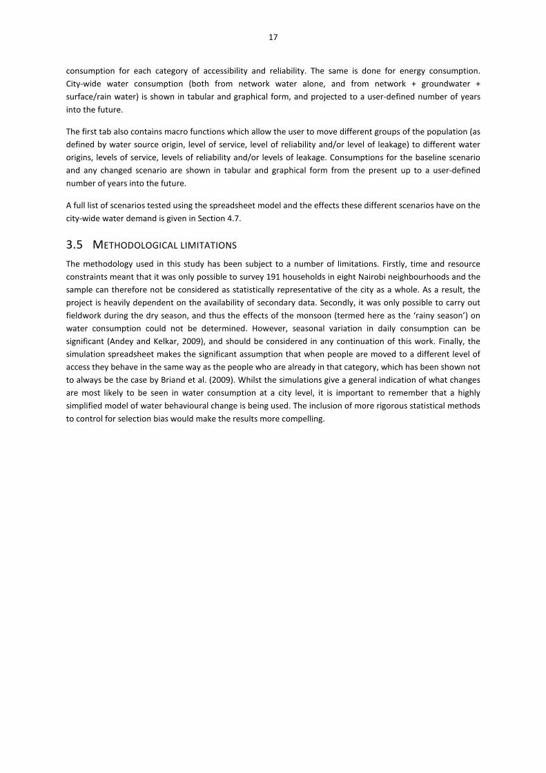
3.5 Methodological limitations ................................................................................................................. 17

4 Fieldwork Results .......................................................................................................................................... 18

4.1 Data cleaning and characterisation ..................................................................................................... 18

4.2 Patterns within the data ..................................................................................................................... 21

4.3 Statistical differences between groups ............................................................................................... 23

4.4 Regression models .............................................................................................................................. 24

4.5 Principal component analysis .............................................................................................................. 26

5 Water use model results ............................................................................................................................... 28

5.1 Characteristic consumption values ..................................................................................................... 28

5.2 Scenario testing results ....................................................................................................................... 29

iv

6 Discussion ..................................................................................................................................................... 31

6.1 Limitations ........................................................................................................................................... 31

6.2 Other options for improving service levels ......................................................................................... 32

7 Conclusions and suggestions for further work ............................................................................................. 33

References ............................................................................................................................................................ 35

Appendix 1: Fieldwork materials .......................................................................................................................... 38

Appendix 2: Variables collected ........................................................................................................................... 48

Appendix 3: Factor Analysis - supporting data ..................................................................................................... 55

TABLE OF FIGURES Figure 1: Price of Water by water source (Bannerjee & Morella, 2011) ................................................................ 6

Figure 2: Mukuru .................................................................................................................................................... 9

Figure 3: Mathare ................................................................................................................................................... 9

Figure 4: Tassia ..................................................................................................................................................... 10

Figure 5: Mowlem ................................................................................................................................................. 10

Figure 6: Kaloleni .................................................................................................................................................. 10

Figure 7: Kayole .................................................................................................................................................... 10

Figure 8: Eastleigh ................................................................................................................................................. 10

Figure 9: Buru Buru Phase 3 ................................................................................................................................. 10

Figure 10: Nairobi ................................................................................................................................................. 11

Figure 11: Fieldwork Site Locations ...................................................................................................................... 11

Figure 12: Simulation spreadsheet, results tab .................................................................................................... 15

Figure 13: Simulation spreadsheet, population and service levels tab ................................................................ 15

Figure 14: Simulation spreadsheet, consumption and energy tab ....................................................................... 16

Figure 15: Histogram of average water consumption in litres per capita per day ............................................... 19

Figure 16: Histogram of log-transformed average water consumption in litres per capita per day .................... 19

Figure 17: Histograms of average water consumption disaggregated by access method ................................... 19

Figure 18: Scatterplot of average water consumption and household wealth score ........................................... 20

Figure 19: Theoretical relationships determining water consumption ................................................................ 23

Figure 20: Scenario results ................................................................................................................................... 30

v

LIST OF TABLES Table 1: Accessibility and reliability of water supplies ........................................................................................... 1

Table 2: Residential characteristics of study sites .................................................................................................. 9

Table 3: Access method for primary source of water ........................................................................................... 18

Table 4: Correlation matrix ................................................................................................................................... 22

Table 5: Difference in means between water source categories, with significant differences highlighted ......... 24

Table 6: Model 1 characteristics ........................................................................................................................... 25

Table 7: Model 2 characteristics ........................................................................................................................... 25

Table 8: Rotated coefficients pattern ................................................................................................................... 26

Table 9: Average consumption values and city-wide population distribution by source used for model ........... 28

vi

ABBREVIATIONS

ABM – Agent-Based Modelling

CAS – Complex Adaptive Systems

CBO – Community Based Organisation

CWS – Continuous Water Supply

DHS – Demographic Health Survey

GIS – Geographic Information Systems

GWOPA – Global Water Operators’ Partnerships Alliance

IFRA – The French Institute for Research in Africa

IWS – Intermittent Water Supply

JMP – Joint Monitoring Programme

Ksh – Kenyan Shillings

KMO – Kaiser-Meyer-Olkin

KNBS – Kenyan National Bureau of Statistics

lpcd – litres per capita per day

NCWSC – Nairobi City Water and Sewerage Company

NRW – Non Revenue Water

OLS – Ordinary Least Squares

PCA – Principal Component Analysis

VBA – Visual Basic for Applications

WAG – Water Action Group

WHS – World Health Survey

WSUP – Water and Sanitation for the Urban Poor

1

1 INTRODUCTION Despite access to adequate amounts of clean water being crucial to health and development, there are still 748 million people worldwide without access to improved sources of drinking water (WHO and UNICEF, 2014). The post-2015 development goals indicate that improving access for these remaining people is a global development priority. However, fresh water resources in many regions are simultaneously coming under increasing pressure from factors such as pollution, population growth and climate change (Khatri et al., 2009). Cities in the developing world in particular are growing rapidly whilst their infrastructure struggles to keep pace with the numbers of people it is required to serve. Furthermore, as economies grow and standards of living rise, increasing numbers of people are looking to improve their level of water access and obtain connections to piped water networks (Nauges and Whittington, 2010). According to the Joint Monitoring Programme (JMP), ‘approximately 70% of the 2.3 billion people who gained access to an improved drinking water source between 1990 and 2012 gained access to piped water on the premises’ (WHO and UNICEF, 2014). There is also increasing pressure worldwide on city utility companies to improve their coverage and quality of service (Banerjee and Morella, 2011). As yet it is unclear what effect these changes will have on city water resources, however it is important that projections are made to anticipate and prepare for their results.

This research project aims to quantify the relative impact of improved water service provision in slum areas within the context of a water basin serving a city. Impacts for consideration include the overall volume of water, energy use in water production and overall costs of production. For the purposes of this analysis we are interested in the implications of supply changes in housing areas where regular utility water supplies piped to the home are not available – hence the scope lies beyond slums and may incorporate low-cost public and private housing with legal land tenure in addition to informal and unplanned settlements and temporary shacks. The research question is therefore the following:

If a city improves water services in slum districts city-wide, what will be the increased water requirement, and what is the magnitude of this increase relative to other competing demands? How will the net increase in water

requirement be affected by different implementation scenarios?

Improvements of water supply services can be broken down into two main dimensions: accessibility (e.g. whether the water source is located inside the home, in the yard, or elsewhere) and reliability (e.g. whether water is available for more or less than a certain number of days per week or hours per day, and whether or not these can be predicted in advance). This can be visualised in the table below, which was developed by water@leeds (2013) in order to portray different levels of water supply service and the steps that can be taken to improve them.

TABLE 1: ACCESSIBILITY AND RELIABILITY OF WATER SUPPLIES

Water supply is… Predictable Unpredictable

Available > x days per week

Available < x days per week

Available > x days per week

Available < x days per week

At home Highest level of service

In the yard Increasing accessibility

Delivered to home

Carried to home Increasing reliability Lowest level of service

SOURCE: (WATER@LEEDS, 2013)

2

In most low-income rapidly growing cities in the global south the impact of such improvements is likely to be high, given that a significant proportion of the population reside in slums and informal and low-cost housing areas with very low levels of service. In Dhaka for example it is estimated that as much as 65% of the population within the utility service area do not receive piped water at home from the water utility. A recent review of water infrastructure in Africa estimated that typically utilities provide service in only about 70% of their service area and that demand-side constraints result in fewer than 45% of the population actually connecting ( Bannerjee and Morella, 2011).

Within this context, the main objectives of this project are: firstly, to understand the resultant changes in consumption when populations move between cells in Table 1; and secondly, to find how the population of a city is distributed within Table 1 at the moment. The effects of moving the population of the city around on Table 1 can then be simulated, and the results shown in the context of the city’s water balance. For this study, the city of Nairobi has been selected for use as a case study to examine these objectives.

3

2 HOUSEHOLD WATER CONSUMPTION IN NAIROBI This chapter discusses the challenges of measuring and predicting household water consumption and explores the historic, demographic and geographic background to Nairobi. Discussions of technical, social and institutional aspects of water supply in Nairobi are also presented. This section therefore serves to situate the current study in the context of previous work, in addition to providing background information on the location of interest.

2.1 MEASURING AND PREDICTING HOUSEHOLD WATER CONSUMPTION It has been demonstrated that the quantity of water available to a person has a greater impact on their health than the quality of that water (Howard and Bartram, 2003), and it is therefore commonly accepted that providing adequate quantities of water should be prioritized over water quality. Whilst utility companies often use broad figures to allocate water to various segments of a population (usually depending on housing size or neighbourhood type), corresponding real-world consumption in these areas can be very different. Some groups may consume more, and others less, than their allocated amounts. In Nairobi, for instance, 40% of the total water is used by 7% of the population, whilst 45% of the population consume only 15% of the city’s water (Ledant, 2011a). Although the determinants of water consumption are not fully understood, they can be theorised to result from levels of accessibility and reliability of a water service. Understanding the water demand implications of changing levels of accessibility and reliability is therefore fundamental to carrying out good planning and equitable allocation of water resources (Briand et al., 2009; Nauges and Whittington, 2010). This becomes even more important in water-stressed areas such as Kenya.

Although many studies have been produced concerning household water demand in high-income countries the corresponding body of work for low to middle-income countries is significantly smaller (ibid). One of the factors that make this work particularly challenging is the complex way in which many households in low to middle-income countries access water. Unreliable municipal supplies may lead households to utilise a combination of different sources, service providers, and technologies (ibid). For example, a household that receives water unreliably from the network may also opt to purchase groundwater from kiosks or neighbours at times when mains piped water is not accessible, or if the quality is perceived to be unsuitable for drinking. This makes analysing household water demand in these circumstances a far more challenging task than for users who generally access water from the network of one sole provider (Mu et al., 1990).

Another complication is the mismatch between demand and consumption when water supply falls short of requirements. In high-income countries, for the most part, demand equals consumption. However, a large number of cities in low to middle-income countries lack the water resources and/or infrastructural requirements to transfer an adequate amount of water to their population in order to meet total demand (Khatri et al., 2009). Water might therefore be rationed, and distributed to various different parts of the city on a daily or weekly basis. Consumption may consequently be different to demand if households lack the ability to store enough water for periods when the networked supply is not available. For unconnected households, other factors such as distance to source, queueing time, and inflated kiosk prices may result in a household's water consumption being less than their ideal water demand (Olajuyigbe, 2010). If these factors are altered so as to improve the accessibility of a water supply, we might expect consumption to then rise to meet demand.

2.2 CITY OF NAIROBI 2.2.1 OVERVIEW Nairobi is the capital city of Kenya and the commercial, financial and diplomatic hub of East Africa (UN Habitat, 2006). The city began as supply depot in 1899 during the construction of a railway stretching from the coast to Uganda (NCC, no date (a)). Since then, the population has swelled to over 3.5 million people (NCC, no date (b)) and continues to grow at a rate of 2.8% per year (UN Habitat, 2006). The city employs around a quarter of the

4

Kenyan work force and generates over 45% of the country’s GDP, but it is also characterised by high rates of poverty, extreme inequality, poor health outcomes, significant levels of crime and inadequate provision of basic services (UN-Habitat 2006 p.4). Whilst many of these problems have had a long history, rapid population growth in recent years has been an important exacerbating factor. It is estimated that up to 60% of the population reside in informal settlements, which cover just 5% of the city’s land area (ibid). Nairobi employs 43% of all urban workers in Kenya, however the majority of employment is found within the informal sector (ibid).

Much of the population growth has been concentrated in large informal settlements. Indeed, approximately 60% of Nairobi’s population now live in such locations (Crow & Odaba 2010). The informal settlements can have a population density 100 times as high as those of some of the wealthier neighbourhoods and many of their residents live below the poverty line (Graf et al., 2008; UN-Habitat 2006). The high rates of poverty are matched by poor provision of basic services including water, sanitation, electricity, waste disposal and health care, partly due to stretched capacity, partly due to poor urban planning, and partly due to the illegal status of many of the houses.

Whilst the inadequacies of such provisions are especially stark in informal settlements, they are not exclusive to them. Water provision in particular has long been considered poor even in the more affluent areas of the city. A 2005 survey of 674 households from a cross section of residential settlements and socioeconomic groups found that – by a substantial distance – improving Nairobi’s water supply was seen as the most pressing need the city has (Gulyani et al. 2005b).

2.2.2 INSTITUTIONAL FRAMEWORK The institution with responsibility for water supply in Nairobi is the Nairobi City Water and Sewerage Company (NCWSC) which was created after the Kenyan Water Sector underwent significant reforms in 2002 (NCWSC, 2011a). Major features of these reforms were corporatisation of water supply and the separation of policy-making, service delivery and regulation. Assets are owned by the Athi Water Services Board, whilst service delivery is carried out by NCWSC, which is a subsidiary of Nairobi City Council (ibid). The Water Services Regulatory Board (WASREB) was also set up as part of the 2002 reforms as an industry watchdog, and runs community-level Water Action Groups (WAGs) to assist customers in following up on unresolved water complaints (WSP, 2011).

This institutional framework was established in 2004, with Nairobi City Council having previously managed provision of water services in the city. The creation of the AWSB and NCWSC were part of an attempt by the government of the time to create a more commercially focused and financially sustainable water sector, free from political interference (Gulyani et al. 2005a). Prior to 2004, the financial and commercial management of water services had been criticised for being poor, and maintenance and capital expenditure had been on the decline (Gulyani et al. 2005a; Werna 1997). By creating a water company autonomous from the council, it was felt that there would be a greater commercial incentive to improve efficiency, develop infrastructure and drive up service quality (Crow & Odaba 2010).

2.2.3 WATER RESOURCES & SYSTEM CAPACITY Nairobi sources the vast majority of water from dams located up to 50km to the north of the city in other counties (NCWSC, 2011b). A small amount is also drawn from groundwater sources both within and outside the city boundaries (ibid). Since it was completed in 1994, the Thika Dam has been the city’s main source, supplemented by water from the Sasumua and Ruiru Dams, the Kikuyu springs and several hundred of boreholes dotted around the city itself (NCWSC 2013). Supply is estimated at 580,000 m3 per day (Athi Water Services Board, 2006) however NCWSC only receives revenue for around 60% of this amount (Ledant, 2011a). Around half of all water losses are estimated to be commercial losses whilst the other half are physical losses (ibid). Due to inadequacies in current monitoring methods, data on flows and usages is considered unreliable, making it difficult to precisely assess the losses or to trace them back to their origin (Gulyani et al., 2005a).

5

Supply does not meet demand, which is projected to increase over the coming years (Athi Water Services Board, 2006). Nairobi therefore employs a rationing programme, whereby water is rotated to different areas of the city on a weekly basis. A project of large-scale infrastructural investments to improve water supply is underway, with short-term demand expected to be met by around 2017 (ibid). However, this requires sourcing water from ever-further catchments.

The future of Nairobi’s water supply from the stand point of resource availability is uncertain. Siltation of the reservoirs which currently act as the city’s main source will gradually reduce existing capacity, whilst political factors and conflict are potential threats in the future.

2.2.4 DISTRIBUTION SOURCES Basic services have struggled to keep up with the rapid population growth that has taken place in Nairobi. Nilsson and Nyangeri Nyanchaga (2008) indicate that this is probably one of the main reasons for the significant decline in service standards since the 1970s. Whilst an estimated 64% of Nairobi’s residents have direct access to piped water either through a yard tap or household tap, it is estimated that 80% of residents in informal settlements do not have any form of connection and must therefore transport water to their properties (Ledant, 2011a; UN Habitat, 2006). They source water from standpipes, kiosks, vendors using handcarts or tankers.

In Nairobi, households make use of an array of different water sources. A survey by Gulyani et al. (2005a p.1252) of households from three Kenyan cities, including Nairobi, reported that 46% of households use private in-house piped connections as their primary source of water, whilst 15% use yard taps. As the reliability and quality of the piped network tends to be poor and because large areas of the informal settlements are not served by the NCWSC’s network, a number of alternative water sources are also widely used (Werna 1997).

In high and middle-income neighbourhoods, water trucks commonly supply households with water to supplement their piped service and a few thousand boreholes are operated by households, farms and businesses (Banerjee & Morella 2011; Gulyani et al. 2005a). In the informal settlements on the other hand, the primary source of water are standpipes and water kiosks. Although a number of community-based organisations also operate them, these kiosks and standpipes are mostly run by private vendors. They are often illegally connected to the NCWSC network and make a profit by reselling the water from the piped system for a higher price. It is believed that around 64% of slum residents rely on buying water from these sources, often using buckets or jerry cans to transport the water between the kiosks and their homes (Gulyani & Talukdar 2008 p.1922). Across all socioeconomic groups, there is a tendency to store large quantities of water in homes to safeguard against shortages and the irregularity of the supply (Crow & Odaba 2010).

The handling of water supply to informal settlements has long been an issue of debate. There has been reluctance within government agencies to allow investment in the slum areas for fear that it will signal tacit approval of the settlements which have often been built illegally (Werna 1997). Furthermore, the continuing threat of removal that many residents face from both the authorities and their landlords (only 8% of residents are owner-occupiers) with whom they often only have informal agreements, means they have little incentive to invest in their own units (Gulyani & Talukdar 2008 p.1920). There is also a belief that improving service provision will lead to gentrification in those areas affected, benefiting landlords but not the current tenants (Gulyani & Talukdar 2008).

2.2.5 WATER CONSUMPTION Per capita water consumption in Kenya is notably low. A survey by Gulyani et al. (2005a p.1252) found that water use averaged about 40 litres per capita per day (lpcd) with a median value of 30 lcd for the three cities in their study. In Nairobi, the mean consumption was found to be 37 lpcd whilst the median was 30 lpcd. These figures are low not just compared to other countries, but also compared with previous consumption in Kenya.

6

Gulyani et al. (2005a p.1252) report that in 1967 consumption was at 105 lpcd, which means a significant decline has taken place.

Perhaps unsurprisingly, there is inequality in water use between socioeconomic groups, though it is not as great as might be expected. The survey by Gulyani et al. (2005 p.1254) found that individuals from poor households use an average of 33 lpcd compared with 44 lpcd for the non-poor. Consumption amongst the wealthiest 11-12% of households is around 30% of the total domestic water supply, showing the disparity in regards to water consumption (UN-Habitat 2006 p.4). It should be recognised that all of these figures are now several years old so changes to consumption patterns might have taken place in the intervening years.

2.2.6 CORE ISSUES Poor reliability, high prices and time spent on collecting water are three of the main problems affecting Nairobi’s residents above and beyond issues relating to access to the piped network (Gulyani et al. 2005a). Poor reliability and occasional shortages characterise the piped water supply. Gulyani et al. (2005a p.1262) report that ‘36% of the households with private connections, 36% of those relying on kiosks and 47% of those with yard taps report that water is available for less than 8 hours per day’. Indeed, only a minority of households with private connections receive water for more than 16 hours a day. In informal settlements like Kibera, water is often completely unavailable on certain days making storage essential (Crow & Odaba 2010). Reservoir shortages can lead to even more reduced service.

The second issue is cost. Although it should be recognised that these figures can fluctuate seasonally and according to supply, Banerjee and Morella (2011, p.166) report that households buying water from water vendors or tankers pay about 20 more for water than those with private connections, as shown in Figure 1. The poor service provision by the utility is therefore forcing households from all socio-economic groups to purchase water at significantly higher prices than they could have if the quality, reliability and accessibility of the piped network was improved.

FIGURE 1: PRICE OF WATER BY WATER SOURCE (BANNERJEE & MORELLA, 2011)

Theoretically, the poor are eligible for a subsidised tariff from the piped network, but because so few have a private connection, they in fact end up paying some of the highest rates of all by having to buy from kiosks. Gulyani et al. (2005a p.1247) found that kiosk operators commonly charge 18 times the price they pay for water. Whilst Crow and Odaba (2010) attribute some of this mark up to the high capital costs traders can incur by laying pipes, buying storage tanks and, often, paying bribes to plumbers and officials for connections to the piped network, substantial profits are still thought to be made. The opening of NGO-run kiosks has apparently put downward pressure on water prices in the areas where they operate (Gulyani et al. 2005a p.1267). However, there remain significant barriers to entry for those looking to set up competing kiosks and other water retail operations in the informal settlements as a substantial proportion of the vendors currently act as a cartel and have sought to protect the exclusivity of their trade (Crow & Odaba 2010 p.741).

$0.0$0.5$1.0$1.5$2.0$2.5$3.0$3.5$4.0

Piped connection Standpipes Water tankers Water vendors

Price of water (US$/m³)

7

The final major issue is the time water collection can take. Again according to the survey by Gulyani et al. (2005a p.1259), households spend an average of 30 minutes a day collecting water. The time spent was found to be 15 minutes for the non-poor and 42 minutes for the poor. Women or children are primarily responsible for the task of collecting water. They can spend an hour or more walking to the vendor, queuing, collecting the water and returning home, often with very heavy loads (Crow & Odaba 2010). Collecting water can consume even more time when additional water is needed for laundry or other uses, and this often limits what else these people can do during the day.

These issues have substantial repercussions for Nairobi’s residents. For many people paying for water accounts for a significant portion of their wages, whilst washing clothes, showering and the number of meals cooked can be curtailed when water is not available or too costly, and disease can spread much more easily when access to water is difficult (Crow & Odaba 2010). For example, diarrhoea amongst children younger than three is around three times more prevalent in Kibera than in Nairobi as a whole (Graf et al. 2008 p.337)

2.2.7 FUTURE It can be seen that there is significant scope for improving water supply for many of the residents of Nairobi. This need however takes place against a background of rapid population growth, poor revenue recovery due to high water losses, and water scarcity. The organisations involved in delivering water to the people of Nairobi face a significant challenge in their attempts to improve access to, and quality of, the service. There also appear to be clear lessons for the providers to learn and important debates to be had, especially when it comes to how water provision should be handled in the informal settlements where a major part of the city’s population lives.

8

3 METHODOLOGY

3.1 SECONDARY DATA REVIEW Secondary data was reviewed to identify spatial patterns of water access across Nairobi and to obtain general background information about the city. The review covered both academic and grey literature, and gathered a number of micro-datasets which are described below:

Kenyan Census

The Kenyan National Census was most recently produced in 2009 by the Kenya National Bureau of Statistics (KNBS) and the Ministry of Planning (KNBS, 2014). The census covered a total of 909,589 households across Kenya, is available to download and can be disaggregated to sub-location level. As part of the census, households are asked to identify their main source of water from a number of options. This data was used to populate the simulation spreadsheet (described in Section 3.4) with the numbers of people using certain water access categories at a district level.

Access to Water in Nairobi – GWOPA and IFRA

The Global Water Operators’ Partnerships Alliance (GWOPA) and the French Institute for Research in Africa (IFRA) Nairobi carried out a study in 2011 with the goal of mapping inequality in water and sanitation access at a sub-city level (Ledant, 2011a). This involved splitting Nairobi’s neighbourhoods into a number of residential categories, which were then representatively sampled by household questionnaire (Ledant, 2011b). Residential categorisation was done using high-resolution satellite imagery and computer algorithms which grouped similar areas based on characteristics such as: plot size, ratio of public to private space, population density, and tree cover (ibid). Household questionnaires covered information on: household water source and consumption, cost per litre of water, percentage of household income spent on water, and sanitation type. Over 800 households were interviewed and the raw data was very kindly made available for use in this project. This data was used to select fieldwork sites so as to cover a wide range of water access patterns.

Demographic Health Survey - Kenya

The Demographic Health Survey (DHS) is designed to monitor health and population issues, and was most recently carried out in Kenya in 2008-09 (KNBS and ICF Macro, 2010). A total of 1108 households were surveyed within the urban areas of Nairobi region. As part of the survey, respondents were asked to specify their drinking water source, household-use water source, and the time taken to collect water (ibid). Micro-data can be disaggregated to household level and sorted by region. This data was used to triangulate water access patterns from census data and gain further information on access categories which were not covered in the census, such as water delivered by handcarts.

3.2 FIELDWORK Fieldwork was carried out in Nairobi for 3 weeks in April 2014 by researchers from the University of Leeds, and a number of Kenyan partners with local expertise and data collection experience. The purpose of the fieldwork was to ground-truth secondary data on spatial access patterns, and gather average consumption information and demographics for different water access categories. Fieldwork techniques included: household questionnaires, water point observations, focus groups and expert interviews. Sample sizes were not large enough to be statistically representative of the entire city due to time and resource constraints. However, the results are still of indicative value and can be used to show trends as well as patterns in the data.

9

3.2.1 HOUSEHOLD QUESTIONNAIRES Secondary data was used to obtain a preliminary picture of water access patterns in different neighbourhoods, and eight were then selected for surveying. Neighbourhoods studied are described in Table 2, and shown in Figures 2 to 9.

TABLE 2: RESIDENTIAL CHARACTERISTICS OF STUDY SITES

Neighbourhood Name Residential Typology Characteristics Mukuru Mathare Tassia

Areas characterised by high-density, unplanned, low-quality housing

Roof cover >85% corrugated iron sheets Tree cover <3% Built up space >37% Public space <20%

Mowlem Area characterised by low density, low quality housing

Roof cover >85% corrugated iron sheets Tree cover <3% Built up space >37%

Kaloleni Area characterised by collective housing with open access

Tree cover >3% and <13.5%

Kayole Area characterised by high density, low quality, planned housing

Roof cover >85% corrugated iron sheets Tree cover <3% Built up space >37% Public space >20%

Eastleigh Area characterised by high density multi-storey buildings

Tree cover <3%

Buru Buru Phase 3 Area characterised by dense, individual housing

Tree cover >3% and <13.5% Plot size >190m2

SOURCE: (LEDANT, 2011B), MODIFIED BY AUTHOR.

These neighbourhoods were selected using data gathered by the GWOPA and IFRA study, and aimed to represent maximum diversity in terms of access to water. A variety of other residential characteristics were also displayed, such as: population density, piped water and sewer access, average income, plot size, average water consumption and average water cost. All eight neighbourhoods were chosen from the eastern part of Nairobi, as shown in Figures 10 and 11, as this was identified to be the part of the city showing the greatest diversity in terms of these characteristics.

FIGURE 2: MUKURU

FIGURE 3: MATHARE

SOURCE: AUTHOR’S OWN.

SOURCE: AUTHOR’S OWN.

10

FIGURE 4: TASSIA

FIGURE 5: MOWLEM

SOURCE: AUTHOR’S OWN.

SOURCE: AUTHOR’S OWN.

FIGURE 6: KALOLENI

FIGURE 7: KAYOLE

SOURCE: AUTHOR’S OWN.

SOURCE: AUTHOR’S OWN.

FIGURE 8: EASTLEIGH

FIGURE 9: BURU BURU PHASE 3

SOURCE: AUTHOR’S OWN.

SOURCE: AUTHOR’S OWN.

11

FIGURE 10: NAIROBI SOURCE: (OPENSTREETMAP, 2014). ©OPENSTREETMAP CONTRIBUTORS.

FIGURE 11: FIELDWORK SITE LOCATIONS SOURCE: (OPENSTREETMAP, 2014). ©OPENSTREETMAP CONTRIBUTORS. MODIFIED BY AUTHOR.

Tassia

Mathare

Mowlem

Mukuru

Kaloleni

See Figure 10

12

A total of 191 household questionnaires were carried out in the eight neighbourhoods described above to gather information on water accessibility, reliability and consumption patterns. Copies of the questionnaires used, interviewer guidelines and information sheet are given in Appendix 1. Questionnaires were written in English, but administered by persons fluent in both Swahili and English (which are both official languages of Kenya).

Key variables gathered include:

Demographics; Household characteristics; Primary, secondary and tertiary sources of water for drinking and household uses; Average daily consumption of water; Time taken and distance travelled to collect water; Cost of water; and Water storage available within the household.

A full list of variables is provided in Appendix 2. Household wealth was approximated by completing a separate questionnaire based on the approach used in the most recent DHS survey of Kenya, which gathered information on household income indicators. The advantages and disadvantages of this method are discussed further in Section 3.2.2.

As asking respondents about their water use in litres per day would likely not lead to accurate data, consumption for users collecting water was estimated by the interviewers by establishing the size of containers and the number of times they are filled per day. This was cross-checked and triangulated with the expenditure on water and daily or weekly water usage by activity. For those with household connections and yard taps, the consumption was calculated by estimating the size of storage containers and the number of times they are filled per day or week. However, had been observed that many respondents with piped connections seemed unsure of their water consumption and found it difficult to make an estimation of average consumption off-hand. Therefore, consumption values for these groups were back-calculated using their average monthly water bills and the NCWSC tariff, and checked against stated consumption values, as well as water usage by activity. The interviewer guidelines on how to estimate quantities are given in Appendix 1.

3.2.2 HOUSEHOLD WEALTH ASSESSMENT Household wealth – as assessed using proxy variables of asset ownership – has been proven to be a more robust indicator of the financial stability of a household than income (Rutstein and Johnson, 2004), and was therefore the method chosen to estimate the finances of households for this study. The method involves asking households to identify from a list which assets they own, recording the number of people per sleeping room, and observing housing materials. The list of assets used as income indicators is termed the ‘wealth index’, and ranges from basics such as a bed, tables, and chairs to more expensive items such as washing machines and refrigerators. A wealth score for each household is derived from the wealth index by assigning weightings to each item through Principal Component Analysis (PCA), which is a statistical technique designed to identify underlying patterns in a large number of variables. These weightings are then multiplied with the value of the variable (which could be a binary value of ‘1’ for ‘owned’ and ‘0’ for ‘not owned’, or a numerical value such as ‘3 people per sleeping room’) and the results are summed to produce the wealth score for each household.

It is also important to acknowledge that the way in which an asset represents wealth can be very country-specific; for example, a bicycle may not have the same value in a mountainous country as in a flatter country (Rutstein and Johnson, 2004). For this study, the asset list for the income indicators questionnaire was taken from the most recent DHS survey in Kenya, to ensure that the list was appropriate for the country.

13

The wealth index method avoids a number of disadvantages to measuring a household’s financial stability by asking the respondent to state their average income. Firstly, income might fluctuate significantly if the main earner is unemployed or employed in the informal sector. Households might also feel an incentive to overestimate or underestimate their average earnings, or simply not know them. In some cases, members of the household may have incentive to not divulge extra earnings to each other and thus the total household income may not be revealed by the respondent. However, whilst having a number of advantages, the wealth index method was difficult to implement in the field for a number of reasons. Firstly, it was strongly felt by the translators that asking people in informal settlements whether they owned certain items (such as a washing machine) was insensitive. They also commented that it was disheartening for a household to have to admit to not owning a large number of items on the list. Eventually, translators only asked households whether they owned items that were considered likely to be present within that neighbourhood (so nobody in the informal settlements was asked whether they owned a refrigerator, freezer or washing machine) as not to cause embarrassment or discomfort. Whilst considered unlikely, this may have had the effect of distorting the scores as households owning unusual assets within a neighbourhood would not have been identified. Secondly, some households were reluctant to complete the wealth index questionnaire as they felt that the information was unnecessary and unrelated to the purpose of the interview. They may also have felt that revealing this information could make their property vulnerable to theft. This problem could have been avoided by the fieldworkers providing a more detailed explanation of why the questions were necessary.

Analysis and interpretation of the income indicators was performed using a similar method to that used by the DHS (Rutstein and Johnson, 2004). Income Indicator data was entered into a Microsoft Excel spreadsheet using binary form for all dichotomous variables. Those variables for which all households had a positive/negative score were excluded, as these would not contribute any information on the relative differences between households in the sample. Factor analysis was then run on all variables using the principal components method available in the statistical software package SPSS, version 22. Only one factor was extracted. The resulting wealth scores were then divided into wealth categories using the k-means clustering tool available in SPSS. Wealth categorization by clustering is viewed as superior to the traditional method of categorization by quintiles (as used by the DHS), because it allows the formation of natural groups rather than artificially separating households who might otherwise be very similar (Hoque, 2014). A total of 5 wealth categories were created, and both the raw wealth scores and wealth categories were examined as household-specific variables when analysing water consumption patterns.

3.2.3 WATER POINT OBSERVATIONS 15 water point observations were carried out in the informal settlements of Mukuru, Mathare and Tassia, between the hours of 9 a.m. and 4 p.m. Data gathered in the water point observations was used to triangulate answers from household questionnaires concerning the amount of time devoted to collecting water (which was generally underestimated). The water vendors for each water point were also interviewed using the same household questionnaire as administered to the rest of the sample. The following was observed for a period of 15-20 minutes:

The number of people coming to collect water; The average number and size of containers carried by each person; The average length of time taken to fill containers (hence estimating the flow rate); and The gender and age of people collecting water.

3.2.4 FOCUS GROUPS Focus groups were carried out in Mukuru and Mathare, each with 6 participants from community-based organisations (CBOs) who are involved in water, sanitation and hygiene service delivery. Information gathered in the focus group was subsequently used to refine the household questionnaires by adding a specific question to enquire about water consumption resulting from laundry, which was highlighted as one of the main water

14

uses in the household. This had the effect of highlighting large amounts of additional water that were being used on a weekly basis, and hence increasing average consumption values recorded per capita.

During the focus groups, participants were asked to discuss the following:

Main uses of water in their households; Average amount of water used per day; Effects of young children on water consumption; Who in the household is responsible for collecting water; Differences in cost and accessibility of water in the dry and wet seasons; How water shortages are dealt with; and The impact of hypothetical increases/decreases in cost, accessibility and reliability.

Questions were asked in both English and Swahili, whilst two note takers recorded both English and Swahili responses.

3.2.5 EXPERT INTERVIEWS Expert interviews were conducted in order to ascertain information about the NCWSC network and planned improvements to it. The following people were interviewed:

Ms. Eden Mati and Mr. Gerald Maina – WSUP Kenya; Mr. John Chege – NCWSC, Informal Settlements Department; Mr. Kagiri Gicheha – NCWSC, Distribution Department; Mr. Mburu Kiemo – NCWSC, Non-Revenue Water Department; Mr. Martin Kareithi – NCWSC, Geographic Information Systems (GIS) Department; and Mr. Boniface Kagwe – Nairobi Water Action Group, Chair.

During these interviews, the following documents and files were also made available to the project team (N.B. unless stated otherwise, these files are not generally publically available):

Reports discussing the implementation of a pre-paid meter pilot project carried out in Nairobi by WSUP Kenya;

GIS layers for the Nairobi water and sewerage network and administrative boundaries; Maps of the Nairobi water and sewerage network and administrative boundaries; A spreadsheet showing the Nairobi water balance, including a breakdown of NRW; The rationing schedule for the Nairobi water network (publically available); and The current tariffs charged by NCWSC (publically available).

3.3 DATA ANALYSIS Once data had been collected, the ranges and averages of variables (categorical and continuous) were checked and outliers flagged and/or removed. Consumption data was aggregated for each household and converted to units of litres per capita per day (lpcd).

Data analysis involved the following:

Data cleaning and characterisation; Identifying correlations within consumption-related variables; Checking for statistical differences in consumption between access categories; Constructing regression models with consumption as the dependent variable; Calculating average consumption values for each level of access; Carrying out factor analysis on consumption-related variables to identify patterns; and

15

Triangulating findings with previous work.

3.4 SCENARIO TESTING A spatial picture of Nairobi’s domestic water consumption can be constructed at a sub-city level using data on the percentages of Nairobi’s population falling into different access categories, and the average consumption values of people within these access categories. Water supply improvement scenarios were then simulated by moving groups of the population from one access category to another. Scenario testing was carried out using a purpose-built spreadsheet created by the project team in Microsoft Excel 2013, containing macros written in Visual Basic for Applications (VBA). Screenshots of the spreadsheet are shown in Figures 12, 13 and 14.

FIGURE 12: SIMULATION SPREADSHEET, RESULTS TAB

FIGURE 13: SIMULATION SPREADSHEET, POPULATION AND SERVICE LEVELS TAB

16

FIGURE 14: SIMULATION SPREADSHEET, CONSUMPTION AND ENERGY TAB The spreadsheet contains three tabs:

1. Results; 2. Population and service level information; and 3. Consumption and energy information.

The tabs are described in the order in which the user inputs information.

The third tab (Figure 13) contains set-up information concerning characteristic values of consumption, energy usage, population growth and leakage. All of these parameters can be modified, allowing the spreadsheet to be tailored to the characteristics of a particular area. Firstly, details of the average water consumption in lpcd for different levels of service and reliability are entered into a table. Information concerning the average energy cost in kilowatt hours per litre (kWh/l) for mechanised and un-mechanised methods of delivering water from three types of origin (water company network water, ground water and surface/rain water) is entered into a second table. Finally, values for three categorized rates of population growth and leakage (high, medium and low) can be defined.

The second tab (Figure 12) sets up a model of the population of the city with population groups assigned to different service levels, population growths, water leakage rates and water source origins. There is no limit to how much detail it is possible to include in this tab; the only constraint is the availability of data for accurate input. The model can be constructed at a city-level, district-level, or at smaller units of location. For each unit, a row is created to describe each unique mode of water access within that location. If the population of a location displays homogenous characteristics of water access (for example, everyone accesses water from the utility network at the same level of reliability and leakage, and the area has a relatively uniform population growth) then only one row is needed. However, if the population utilises a multitude of water access methods, with different levels of reliability, leakage and population growth then several rows are needed to describe all groups.

The first tab (Figure 11) displays the results of the simulation. Firstly, an overall view of which proportion of the city’s population lies in each access category is shown. The model then takes each row of the second tab and multiplies the population present in that row by the characteristic water consumption and energy use for that row, as defined by the values in the third tab. The results are then aggregated to show the total water

17

consumption for each category of accessibility and reliability. The same is done for energy consumption. City-wide water consumption (both from network water alone, and from network + groundwater + surface/rain water) is shown in tabular and graphical form, and projected to a user-defined number of years into the future.

The first tab also contains macro functions which allow the user to move different groups of the population (as defined by water source origin, level of service, level of reliability and/or level of leakage) to different water origins, levels of service, levels of reliability and/or levels of leakage. Consumptions for the baseline scenario and any changed scenario are shown in tabular and graphical form from the present up to a user-defined number of years into the future.

A full list of scenarios tested using the spreadsheet model and the effects these different scenarios have on the city-wide water demand is given in Section 4.7.

3.5 METHODOLOGICAL LIMITATIONS The methodology used in this study has been subject to a number of limitations. Firstly, time and resource constraints meant that it was only possible to survey 191 households in eight Nairobi neighbourhoods and the sample can therefore not be considered as statistically representative of the city as a whole. As a result, the project is heavily dependent on the availability of secondary data. Secondly, it was only possible to carry out fieldwork during the dry season, and thus the effects of the monsoon (termed here as the ‘rainy season’) on water consumption could not be determined. However, seasonal variation in daily consumption can be significant (Andey and Kelkar, 2009), and should be considered in any continuation of this work. Finally, the simulation spreadsheet makes the significant assumption that when people are moved to a different level of access they behave in the same way as the people who are already in that category, which has been shown not to always be the case by Briand et al. (2009). Whilst the simulations give a general indication of what changes are most likely to be seen in water consumption at a city level, it is important to remember that a highly simplified model of water behavioural change is being used. The inclusion of more rigorous statistical methods to control for selection bias would make the results more compelling.

18

4 FIELDWORK RESULTS This chapter begins by noting preliminary observations from the data and subsequent decisions on data processing, before presenting the results of data analysis and discussing their significance.

Out of the households surveyed, 98% used the same water source to obtain both drinking water and water for household uses. Furthermore, 92% of households specified primary water sources only, and no households specified tertiary water sources. It was therefore decided that for analytical purposes it would be sufficient to treat each household as obtaining all their water from a single source. In the service level table given in section 1, a distinction is made between water availability being predictable or not. In our surveyed sample, 86% of respondents stated that their water supply is predictable. For the remaining 14%, the fieldwork team also had some doubts on whether or not the question was understood as intended. It was therefore decided to collapse the categories of predictability, due to these reasons and also to avoid splitting the already small sample size into more categories.

Fieldwork was carried out in the dry season and it was considered that asking people to retrospectively gauge their water consumption during a different season was not a reliable way of measuring water consumption. Therefore, only data for the dry season has been used further.

4.1 DATA CLEANING AND CHARACTERISATION After data cleaning, a total of 124 interviews were used in the final analysis. Outliers were removed by visually inspecting box plots and histograms of consumption data.

Out of the 124 interviews considered for further analysis, 101 were conducted with female respondents and 23 with male respondents. The ages of respondents ranged between 18 and 60, with 44% of respondents falling into the first age bracket of 18-30. Out of all respondents, 90% rented their properties, and 10% were owners. The number of respondents in each access category is shown in Table 3 below.

TABLE 3: ACCESS METHOD FOR PRIMARY SOURCE OF WATER

Access Method Frequency Percent Cumulative Percent Carried to property 55 44.4 44.4 Delivered to property 11 8.9 53.2 In yard 31 25.0 78.2 In dwelling 27 21.8 100.0 Total 124 100.0

Average consumption data for all households has a mean value of 40.9 lpcd, a median value of 31.4 lpcd, and ranges from 4.8 lpcd to 208.0 lpcd. This is comparable to the average water consumption for urban Kenyan households stated in another study examining domestic water use in East Africa - Drawers of Water II – which found a mean value of 45.2 lpcd (Thompson et al., 2001).

A histogram of average consumption (Figure 15) shows that the distribution is strongly skewed to the left, with a skewness value of 2.467 and a kurtosis value of 8.268. A log-10 transformation of average consumption gives a normal distribution, as shown in Figure 16. Figure 17 shows water consumption histograms disaggregated by water source category.

19

FIGURE 15: HISTOGRAM OF AVERAGE WATER CONSUMPTION IN LITRES PER CAPITA PER DAY

FIGURE 16: HISTOGRAM OF LOG-TRANSFORMED AVERAGE WATER CONSUMPTION IN LITRES PER CAPITA PER DAY

FIGURE 17: HISTOGRAMS OF AVERAGE WATER CONSUMPTION DISAGGREGATED BY ACCESS METHOD

20

Water consumption for the whole sample can be seen to follow a reasonably smooth distribution, without clumping around particular values. However, histograms of consumption disaggregated by water source show that lower levels of access (i.e. water is carried to the property, delivered to the property, or in the yard) tend to be concentrated around a certain range, whilst piped water at home displays the largest range of all access modes.

The relationship between average consumption and household wealth score is shown in Figure 18. Markers are coloured by household water source.

FIGURE 18: SCATTERPLOT OF AVERAGE WATER CONSUMPTION AND HOUSEHOLD WEALTH SCORE

Several observations can be made from Figure 18. Firstly, there is some indication of a linear relationship between average consumption and wealth. A regression analysis suggests a positive relationship (as is intuitively sensible), with r=.362 and p=.000. This relationship is therefore significant (i.e. highly unlikely to have occurred by chance); however only 12.4% of variation in the consumption data can be explained by wealth (i.e. the adjusted R square value is .124). This suggests that other variables are also important in determining the water consumption.

A second observation is that water-carrying is the predominant mode of access for those with lower wealth scores, whilst household taps are the predominant mode of access for those with higher wealth scores. Yard taps and delivered water appear as a mode of access towards the middle of the wealth scores.

A third observation (which is corroborated by the histograms in Figure 17) is that consumption values for those who carry water tend to be strongly clustered, with a mean value of 27.8 lpcd and a standard deviation of 12.2. The standard deviation for those who carry water is considerably lower than the corresponding figure for those with a water source in the dwelling (52.2) and also lower than the corresponding figures for those with a

21

water source in the yard and those who have water delivered (21.6 and 22.4, respectively). It seems intuitively sensible that greater variation in consumption should be seen with increased ease of access (and also with increased wealth), as those with more resources might be freer to choose from a greater variety of lifestyles. It also seems intuitive that the time limitations and the physical strain involved in carrying water to a dwelling would place an upper bound on the level of water consumption to be achieved.

A fourth observation is that whilst average consumption values tend to rise with increased ease of access, it is the upper bound of consumption that rises and not the lower. It might therefore be suggested that ownership of a tap is necessary, but not sufficient, to indicate increased water consumption.

4.2 PATTERNS WITHIN THE DATA A correlation matrix was produced to show the relationships between all variables that were considered important, and is shown below in Table 4. Variable relationships which are significant at the p<0.01 level are coloured in pink, whilst variables relationships which are significant at the p<0.05 level are coloured in yellow.

It can be seen that there are a number of strong correlations within the data, but none with a Pearson Correlation value (r) of greater than .8 which suggests that multi-collinearity is not likely to be a problem within the dataset (Pallant, 2005).

The strongest correlations observed, which all had an r value =>.550, were found to be positive relationships between: wealth score and neighbourhood category (r=.673); wealth score and water source category (r=.655); and water source category and neighbourhood category (r=.583). The strongest significant relationship for the average consumption variable was found to be with water source category (r=.443). Significant (but not so strong) relationships were also found to exist with wealth score (r=.362) and neighbourhood category (r=.366). It is notable that variables for number of children, number of infants, education category, ownership of property, and length of time resident in property did not appear to have any significant effect on water source or consumption.

A partial correlation was carried out to assess the strength of the relationship between water consumption and wealth score whilst controlling for water source category. Before controlling for water source category, the correlation between water consumption and wealth score is positive, moderately strong and significant (r=.362, p=.000), however after controlling for water source, this correlation becomes insignificant and weak (r=.107, p=.239). On the other hand, a partial correlation to assess the strength and direction of the relationship between water consumption and water source category was relatively unchanged by controlling for wealth score (relationship prior to controlling: r=.443, p=.000; relationship after controlling: r=.292, p=.001). This suggests that higher wealth leads to better accessibility which in turn leads to higher consumptions, but higher wealth itself is not associated with higher water consumption if the water source is unchanged. Water sources with higher accessibility however seem to lead to a higher average consumption, even if wealth is unchanged.

23

TABLE 4: CORRELATION MATRIX

Wealth Score

Water Source

Category

Property has a

flush toilet

Distance to source (metres)

Water is included in rent

Cost of 20 litres of water

(Ksh)

Average consumption

of water (lpcd)

Neighbour-hood

Category

Reliability in days

per week

Age Category

Number of people in

the household

Length of time

resident in property

Household owns

property

Time to collect

(minutes)

Available volume of storage on property (litres)

Number of children in

the household

Education Category

Number of infants in the household

Wealth Score Pearson Correlation 1 .655 .412 -.381 .325 -.213 .362 .673 -.137 .007 .309** .210* .086 -.206* .289** .139 .195* .032 Sig. (2-tailed) .000 .000 .000 .000 .018 .000 .000 .132 .935 .000 .021 .341 .028 .001 .123 .030 .724

Water Source Category

Pearson Correlation .655 1 .371 -.361 .417 -.456 .443 .583 -.295 -.075 .159 -.105 -.110 -.105 .199* .115 .085 .097 Sig. (2-tailed) .000 .000 .000 .000 .000 .000 .000 .001 .410 .077 .253 .222 .263 .027 .202 .347 .282

Household has a flush toilet

Pearson Correlation .412 .371 1 -.245 .199 -.132 .252 .333 -.047 -.067 .128 -.083 -.084 -.047 .200* -.010 .076 .062 Sig. (2-tailed) .000 .000 .016 .030 .152 .006 .000 .615 .466 .164 .375 .363 .627 .029 .915 .413 .504

Distance to source (metres)

Pearson Correlation -.381 -.361 -.245 1 -.232 .256 -.181 -.115 .006 .113 -.053 -.031 .018 .400** -.151 -.083 -.097 .007 Sig. (2-tailed) .000 .000 .016 .020 .010 .070 .257 .949 .259 .595 .763 .862 .000 .132 .410 .337 .948

Water is included in rent

Pearson Correlation .325 .417 .199 -.232 1 -.527 -.116 .172 -.507 -.149 -.061 -.107 -.156 .079 .001 -.036 .004 .169 Sig. (2-tailed) .000 .000 .030 .020 .000 .201 .058 .000 .098 .502 .247 .083 .399 .994 .689 .969 .060

Cost of 20 litres of water (Ksh)

Pearson Correlation -.213 -.456 -.132 .256 -.527 1 -.121 -.152 .262 .014 -.035 -.042 .078 .119 -.016 -.046 .164 -.081 Sig. (2-tailed) .018 .000 .152 .010 .000 .180 .094 .003 .881 .702 .650 .390 .206 .863 .608 .069 .369

Average consumption of

water (lpcd)

Pearson Correlation .362 .443 .252 -.181 -.116 -.121 1 .366 .108 -.029 .020 -.005 .036 -.033 .125 .042 .094 -.089 Sig. (2-tailed) .000 .000 .006 .070 .201 .180 .000 .237 .745 .826 .956 .688 .723 .166 .647 .300 .325

Neighbour-hood Category

Pearson Correlation .673 .583 .333 -.115 .172 -.152 .366 1 -.157 -.010 .085 .114 .013 -.165 .075 .003 .171 -.026 Sig. (2-tailed) .000 .000 .000 .257 .058 .094 .000 .085 .912 .352 .218 .891 .079 .411 .971 .058 .778

Reliability in days per week

Pearson Correlation -.137 -.295 -.047 .006 -.507 .262 .108 -.157 1 .086 .015 .126 .050 -.243** .065 -.065 -.174 -.168 Sig. (2-tailed) .132 .001 .615 .949 .000 .003 .237 .085 .346 .867 .173 .584 .009 .478 .475 .054 .063

Age Category Pearson Correlation .007 -.075 -.067 .113 -.149 .014 -.029 -.010 .086 1 .208* .433** .278** .138 .043 .219* -.272** -.147 Sig. (2-tailed) .935 .410 .466 .259 .098 .881 .745 .912 .346 .020 .000 .002 .141 .636 .015 .002 .102

Number of people in the household

Pearson Correlation .309 .159 .128 -.053 -.061 -.035 .020 .085 .015 .208* 1 .155 .097 .040 .220* .628** -.168 .214* Sig. (2-tailed) .000 .077 .164 .595 .502 .702 .826 .352 .867 .020 .091 .285 .671 .014 .000 .062 .017

Length of time resident in property

Pearson Correlation .210* -.105 -.083 -.031 -.107 -.042 -.005 .114 .126 .433** .155 1 .345** -.086 .180* .105 -.032 -.160 Sig. (2-tailed) .021 .253 .375 .763 .247 .650 .956 .218 .173 .000 .091 .000 .371 .050 .255 .730 .082

Household owns property

Pearson Correlation .086 -.110 -.084 .018 -.156 .078 .036 .013 .050 .278** .097 .345** 1 -.084 .122 .128 -.001 -.190* Sig. (2-tailed) .341 .222 .363 .862 .083 .390 .688 .891 .584 .002 .285 .000 .372 .177 .156 .987 .035

Time to collect (minutes)

Pearson Correlation -.206* -.105 -.047 .400** .079 .119 -.033 -.165 -.243** .138 .040 -.086 -.084 1 -.085 .079 -.078 .064 Sig. (2-tailed) .028 .263 .627 .000 .399 .206 .723 .079 .009 .141 .671 .371 .372 .367 .404 .406 .495

Available volume of storage on

property (litres)

Pearson Correlation .289** .199* .200* -.151 .001 -.016 .125 .075 .065 .043 .220* .180* .122 -.085 1 -.111 .015 .213* Sig. (2-tailed) .001 .027 .029 .132 .994 .863 .166 .411 .478 .636 .014 .050 .177 .367 .219 .867 .018

Number of children in the

household

Pearson Correlation .139 .115 -.010 -.083 -.036 -.046 .042 .003 -.065 .219* .628** .105 .128 .079 -.111 1 -.182* -.042 Sig. (2-tailed) .123 .202 .915 .410 .689 .608 .647 .971 .475 .015 .000 .255 .156 .404 .219 .043 .644

Education Category

Pearson Correlation .195* .085 .076 -.097 .004 .164 .094 .171 -.174 -.272** -.168 -.032 -.001 -.078 .015 -.182* 1 -.046 Sig. (2-tailed) .030 .347 .413 .337 .969 .069 .300 .058 .054 .002 .062 .730 .987 .406 .867 .043 .612

Number of infants in the household

Pearson Correlation .032 .097 .062 .007 .169 -.081 -.089 -.026 -.168 -.147 .214* -.160 -.190* .064 .213* -.042 -.046 1 Sig. (2-tailed) .724 .282 .504 .948 .060 .369 .325 .778 .063 .102 .017 .082 .035 .495 .018 .644 .612

**. Correlation is significant at the 0.01 level (2-tailed).

*. Correlation is significant at the 0.05 level (2-tailed).

23

To conclude, it could be theorised that the strongest factors in determining a household’s water source are their residential neighbourhood and wealth, and once a source has been established this then becomes the most important variable in determining the amount of water that the household consumes. The relationship between consumption and wealth or consumption and neighbourhood could then be interpreted as secondary, being linked mainly by the choice of water source. This theory is shown visually in Figure 18.

FIGURE 19: THEORETICAL RELATIONSHIPS DETERMINING WATER CONSUMPTION

4.3 STATISTICAL DIFFERENCES BETWEEN GROUPS To see whether differences in the means of water consumption between water source category groups are greater than those occurring within groups and whether they are likely to have occurred by chance, a one-way analysis of variance (ANOVA) test was conducted. The differences were found to be statistically significant (p=0.000), however post-hoc comparisons using the Tukey HSD test showed that significant differences at the p<0.05 level only exist between consumption from taps in dwelling and carried water, and consumption from taps in dwelling and taps in the yard (see Table 5). The difference between consumption from taps in dwelling and delivered water is close to being statistically significant, with p=.066, which can be called a suggestive difference. The Eta squared value for the difference between groups is 0.24, which is classed as a ‘large effect’ by Cohen’s terms (Pallant, 2005).

A two-way between-groups ANOVA was also conducted to check the impact of wealth category and water source category on average water consumption. There was no significant interaction effect between wealth category and water source category (p=0.801), thus indicating that variation of consumption within water source categories is not significantly influenced by wealth category.

24

TABLE 5: DIFFERENCE IN MEANS BETWEEN WATER SOURCE CATEGORIES, WITH SIGNIFICANT DIFFERENCES HIGHLIGHTED

In dwelling (x̅=69.0 lpcd)

In yard (x̅=38.9 lpcd)

Delivered to home (x̅=43.5 lpcd)

Carried to home (x̅=27.8 lpcd)

At home Difference in mean 30.1 lpcd 25.5 lpcd 41.2 lpcd Significance level 0.001 0.066 0.000

In the yard Difference in mean 30.1 lpcd 4.6 lpcd 11.08 lpcd Significance level 0.001 0.968 0.315

Delivered to home

Difference in mean 25.5 lpcd 4.6 lpcd 15.7 lpcd Significance level 0.066 0.968 0.350

Carried to home

Difference in mean 41.2 lpcd 11.08 lpcd 15.7 lpcd Significance level 0.000 0.315 0.350

To determine whether or not reliability (defined as days per week in which water is available) has a statistically significant impact on water consumption, the mean water consumption for two levels of reliability was compared using a t-test. The dataset was split in two groups of users receiving water for more than four days a week and those who get water for four or less days a week. Although there is a difference in the means, it was found to be not statistically significant (p=0.248). This suggests that increased reliability does not necessarily lead to higher water consumptions in the overall sample. Analysing each water source individually shows that for three of the sources, the means for both groups of reliability do not show a statistically significant difference: carried water (p=0.161), delivered water (p=0.923) and household connections (p=0.092). For the yard tap group however, a statistically significant difference could be found (p=0.042). Users of yard taps that are reliable for more than four days per week consume significantly more water than users who receive water for four days or less. However, it needs to be added that the sample size in this category is rather small (n=31), therefore this result should be seen as indicative and would benefit from further investigation in a more rigorous manner using larger sample sizes.

4.4 REGRESSION MODELS Multiple regression models were constructed to produce equations with average per capita water consumption as the dependent variable. The aim was to produce models capable of predicting average per capita water consumption from a set of easily observable household characteristics.

All regression models constructed were statistically significant (p<.001) and did not display any degree of collinearity, however none were able to produce an adjusted R squared value of greater than 0.3 indicating that the models still struggled to explain the majority of variation in the data. The first model was initially produced using 13 variables, and then subsequently refined to remove variables without significance (i.e. p>.005). The models were then tested on the data with two outliers1 removed, to see if this greatly changed the percentage of variation explained.

The initial variables included were: wealth score, age category, time to collect water in minutes, cost of 20 litres of water, household owns property (dummy), volume of storage available on property, number of people in the household, reliability in days per week, distance to source in metres, neighbourhood category, inclusion of water in rent (dummy), and water source category. A model containing all these variables had an adjusted R squared value of .301, however many of the variables contained in the model were insignificant. Refinement of the model to contain significant variables only produced a model with an adjusted R squared value of .289, which contained the variables: wealth score, water source category, and inclusion of water in rent (dummy).

1 Two unusually large values for consumption can be seen at the lower end of the wealth score in Figure 17; these values were not identified as outliers when examining the spread of consumption values alone, but appear to be outliers when consumption is plotted against wealth score.

25

Upon removing outliers, the regression model (using the same variables) produced a lower adjusted R squared value of .254 however the residuals plot produced for this model showed more homogenously distributed residuals, indicating a more valid model. This has been termed ‘Model 1’, and is described below in Table 6. A model using wealth score alone had an adjusted R squared value of .126; this has been termed ‘Model 2’ and is described below in Table 7.

TABLE 6: MODEL 1 CHARACTERISTICS

Coefficient Standard Error p Constant 23.561 4.663 0.000 Wealth score 5.375 2.738 0.052 Water source category 8.328 2.143 0.000 Water included in rent -17.389 4.630 0.000 Number of observations 121 Adjusted R squared value 0.254 Model significance 0.000 Number of case-wise diagnostics 0

TABLE 7: MODEL 2 CHARACTERISTICS

Coefficient Standard Error p Constant 36.338 2.035 0.000 Wealth score 9.558 2.230 0.000 Number of observations 121 Adjusted R squared value 0.126 Model significance 0.000 Number of case-wise diagnostics 1

Regression models are data driven; i.e. the model is derived purely from patterns in the data without any reference to the real-world meaning of the values involved. For this reason, regression models must be constructed with care and the results interpreted with caution. It is also important to remember that the models cannot distinguish between correlation and cause. For instance, it might be surprising to note that having ‘water included within rent’ (as in Model 1) appears to have a negative effect on water consumption, however in practice this may in fact be due to the strong and significant correlation between having yard taps as a water source and having water included in rent (r=.628. p=.000), and the relatively low average consumption of water of yard tap users. Thus, within this particular data set the inclusion of water in rent is correlated with lower average consumption values but does not necessarily cause them. With these limitations, care must be taken not to extrapolate from results without due thought.

It should also be noted that categorical and ordinal variables such as water source and neighbourhood have been allocated quasi-arbitrary values with which to indicate the degree of ease of accessibility, or neighbourhood formality. However, this does not necessarily form a continuous or accurate scale. For example, water access modes are allocated values of 1 – 4, with 1 indicating the least ease of access (carrying water to the dwelling) and 4 indicating the greatest ease of access (having water available in the dwelling). Spacing between these 4 modes of access is not necessarily equidistant and the scale does not take into account the subtleties existing between access modes. For instance, having water delivered to the property is rated as a lower access mode than having a yard tap, but this is down to personal judgement. These issues make these variables not entirely suitable for conducting any kind of correlation or regression analysis, despite them containing highly relevant information. The wealth score, on the other hand, has been produced so as to form a

26

continuous variable. This characteristic makes it more useful in regression analysis than the subsequent categorization into wealth clusters, or other categorized variables. Given the close correlation between wealth score and water source (r=.655, p=.000), wealth score is here considered suitable as a proxy for water source, hence making Model 2 the potentially more useful and robust model. However, for the reasons described, the regression models have not been considered further as they fail to explain the majority of variation in the data and are not considered suitable techniques for this purpose at present.

4.5 PRINCIPAL COMPONENT ANALYSIS Factor analysis techniques such as PCA (as described in Section 3.2.2) are commonly used within the social sciences to develop and evaluate scales of measurement for abstract qualities (Pallant, 2005). PCA was applied to 13 variables considered to be important to water consumption in order to identify important patterns within the dataset and draw out a small number of underlying factors. Prior to performing PCA, the factorability of the data was assessed through Bartlett’s test of sphericity, the Kaiser-Meyer-Olkin (KMO) test, and visual inspection of the correlation matrix, all of which indicated that the data was suitable for this technique (Bartlett’s test: p<0.005 and KMO >0.6) (Pallant, 2005, pp.191). Inspection of the scree plot and the use of parallel analysis (using the free software Monte Carlo PCA for Parallel Analysis (Watkins, 2000)) supported the extraction of 4 independent factors for further investigation. Each factor can be interpreted as a ‘super-variable’ being composed of a number of related variables, with a defined character. The 4 factors explain 61.5% of the variance, with factors 1, 2, 3 and 4 explaining 25.7%, 15.0%, 11.4% and 9.5%% of the variance respectively.

Varimax rotation was performed on the factors to assist with interpretation. This technique rotates the dataset so as to present the pattern of loadings in a way that brings out the underlying nature of the factors more clearly. The rotated solution is shown in Table 8, with significant factor loadings (greater than .3) displayed only, for clarity. A full solution with all loadings displayed, along with the scree plot and other supporting information, is given in Appendix 3.

TABLE 8: ROTATED COEFFICIENTS PATTERN

Component 1 2 3 4

Neighbourhood Category 0.810 Wealth Score 0.758 Water Source Category 0.705 -0.448 Household vends water (dummy) -0.687 0.318 Water is included in rent (dummy) -0.821 Cost of 20 litres of water (Ksh) 0.756 Reliability (days per week water is available) 0.707 -0.303 Age category of respondent 0.730 Household owns property (dummy) 0.696 Available volume of storage on property (litres) 0.566 Number of people in the household 0.417 Time to collect water per day (minutes) 0.824 Distance to water source (metres) 0.737

The four factors can be loosely defined as the following:

1. Degree of asset possession (as determined by source category, wealth score and neighbourhood). 2. Financial elements (such as the cost and payment arrangements for water). 3. Demographics and household characteristics (such as number of people, ownership, size of storage,

and age). 4. Accessibility factors (such as time taken and distance travelled to collect water).

27

There are a few anomalies and unclear relationships within these factors. The presence of ‘household vends water’ and ‘reliability’ within factors 1 and 2 seem out of place, whilst ‘household vends water’ also seems to fit poorly within factor 3. For the most part, however, it would appear that four independent dimensions of water supply have emerged suggesting that further investigation might be worthwhile. The definition of four independent factors covering different aspects relating to water consumption could facilitate the construction of a scale measuring ease of access to water. Such a scale would include a balanced number of questions concerning each of the four identified dimensions - degree of asset possession, financial elements, demographics and household characteristics, and accessibility - which would then be combined into a single continuous scale. A continuous variable of this type might make subsequent analysis of consumption and ease of accessibility more feasible with techniques such as multiple regression.

28

5 WATER USE MODEL RESULTS This section deals with the impacts of changing service levels, which are assessed using the water use model described in section 3.4. As the model requires average consumption values for each level of accessibility and reliability, these are given below before moving on to a discussion of the modelling results.

5.1 CHARACTERISTIC CONSUMPTION VALUES Average consumption values calculated from primary data for different categories of accessibility are presented in Table 9. The distribution of Nairobi’s population within these categories (as determined by the most recent Kenyan census and DHS) is also shown. As these secondary sources do not include any information on reliability, the city-wide users of yard taps were split evenly between the two groups of reliability. This assumption was made to minimise the maximal error and is considered an appropriate level of precision in the context of this study. Surveying statistically representative samples for the groups would enable a more precise estimation of the baseline scenario and are recommended for any further study. As discussed in Section 4.3, a t-test showed a statistically significant difference in mean consumption between different degrees of reliability (expressed in terms of days per week on which water is available) only for yard taps. Therefore the reliability categories have been collapsed into one category for the other water sources. The full range of access categories has been preserved, however it should be noted that one-way ANOVA was unable to detect a statistically significant difference between some of the access categories – the only significant differences were found to be between: carried water and water in dwelling, and yard-tap water and water in dwelling, whilst there was a suggestive difference between delivered water and water in dwelling.

TABLE 9: AVERAGE CONSUMPTION VALUES AND CITY-WIDE POPULATION DISTRIBUTION BY SOURCE USED FOR MODEL

Water Access Source Mean (lpcd)

Median (lpcd) Standard Deviation N in sample N in Nairobi

Carried to property 27.8 25.0 12.2 55 527,426 Delivered to property 43.5 45.7 22.4 11 20,869

In yard <= 4 days per week 33.2 28.6 19.7 21 826,608 > 4 days per week 50.9 58.6 21.5 10 826,608

In dwelling 69.0 60.0 52.3 27 937,854

Average consumption values for unconnected households are similar to those reported by Gulyani et al. (2005), who observed that the average consumption of an unconnected household (i.e. water is carried or delivered) has a mean of 36 lpcd, and a median of 27 lpcd. When weighted to account for the relative prevalence of carried and delivered water throughout Nairobi, consumption data gathered in this study for unconnected households has a mean of 28.4 lpcd and a median of 25.8 lpcd. However, consumption data for connected households (i.e. yard tap or household tap) gathered by Gulyani et al. appears to be lower, with a mean of 37 lpcd and a median of 30 lpcd. The corresponding values for this study are 49.8 lpcd and 40.5 lpcd. The study by Gulyani et al. covered 8 residential sites within Nairobi, interviewing a total of 300 households. It is not known which sites were chosen, except that they were selected so as to ‘ensure inclusion of a wide range of settlement and housing types’. Given that consumption is highly variable, the figures were self-reported by households and only 8 residential sites were examined within Nairobi, it does not seem surprising that there is some discrepancy. Another study examining domestic water use in East Africa (Drawers of Water II) found consumption values for urban Kenya that were much more similar to our own with an average of 47.4 lpcd and 27.7 lpcd for connected and unconnected households, respectively (Thompson et al., 2001).

29

5.2 SCENARIO TESTING RESULTS The impact of various scenarios in which users are moved to higher levels of service were assessed using spreadsheet version 9A (Mac) produced by Dr Andrew Sleigh, which is described in Section 3.4. In total, five scenarios were examined and are described below. All scenarios were extrapolated to 20 years into the future using characteristic population growth rates for each sub-district. Changes to service levels are assumed to take place instantly, meaning that the time of implementation and the gradually increasing water demand is neglected. As the goal of this scenarios testing is to assess the resulting changes in water demand and the final volume of water needed, neglecting the incremental increase in demand during implementation is considered acceptable.

In the scenarios it is assumed that for everyone currently obtaining water from the NCWSC network:

1. Reliability of yard taps was increased to more than four days per week for all current yard tap users; 2. All households with yard tap connections were changed to have household connections; 3. All households with no connections (i.e. water is carried or delivered) were changed to have yard tap

connections with a reliability of up to four days per week; 4. All households with no connections (i.e. water is carried or delivered) were changed to have yard tap

connections with a reliability of more than four days per week and reliability for all current users with yard taps was increased to more than four days per week; and

5. All households with no connections and yard tap connections were changed to have household connections.

In the first run, our model estimated a baseline domestic consumption including physical losses of around 57,500 Ml per year. This was compared with the total amount of water produced according to NWCSC. A water balance for the year 2013 was shared with the research team and showed a total system input volume of 199,432 Ml per year. Commercial and industrial users account for 32% of the overall water demand (IBNet, 2015), which leaves about 135,550 Ml per year for domestic consumption. Therefore, a large gap remained between the initial result and the actual water production. An investigation into average consumption patterns on the sub-city scale showed that consumers in western Nairobi tend to use significantly higher volumes of water than residents in the eastern part of the city. Ledant et al. (2011a) found consumption values of 129 to 288 lpcd in western Nairobi, whilst values in the east tend to be around 30 lpcd. The fieldwork locations used in this study were all located in the east of the city, because of the higher variability of water sources and socio-economics found there, and because this study is focused on improving service levels in poorer, more informal neighbourhoods. To retain the focus on these informal areas, the model was adapted to only include improvements in the eastern neighbourhoods, where consumption values from this study agree with the values found by Ledant et al. (2011a), whilst average water consumption by the population in the west that had been removed from the model was assumed to be 180 lpcd and added to the baseline water use.

This adapted model estimated a baseline water demand of around 120,000 Ml per year, a value within around 15% of the actual production, which can be considered acceptable accuracy. Figure 19 shows the results of the five scenarios described above for the eastern part of the city.

30

FIGURE 20: SCENARIO RESULTS

It can be seen that moving all users with yard taps to a higher level of service by improving their reliability leads to an 11% higher water consumption in eastern Nairobi, which is a 4% increase in city-wide water demand. This is a relatively minor impact on the total demand, but however results in significantly improved services for this group of users.

Providing people currently using yard taps with household taps has a relatively large impact on water consumption, causing water use in the eastern part of Nairobi to rise by 40%, which corresponds to a 12% increase in total water demand. This is caused by the large number of people currently using yard taps, but also means that all of them receive significantly better services after the intervention.

Conversely, the action of moving all users without a network connection onto the lowest form of connection (i.e. a yard tap with low reliability) causes only a very small increase in water consumption, just 2% more than the baseline scenario in the eastern part of town, which is an increase of less than 1% city-wide. If the new users are provided with yard taps with high reliability, the increase is 9% in the eastern part of the city and 3% overall. Thus, providing a yard tap to people who currently access water from the network in any form can be expected to have minimal effects on city-wide water demand, if any at all. It does however significantly increase the level of service to users by reducing the amount of time spent on collecting water every day.

Moving all users without a connection to yard taps with high reliability and improving the reliability for current users of yard taps was found to increase the water demand in eastern Nairobi by 21% and represents an increase of 6% in overall water use. This is a bigger impact, but also provides a higher level of service to users.

Increasing the level of service to a household tap for all people currently accessing water from the network has the highest impact, it increases water consumption in eastern Nairobi by 50%, which is a 15% increase in city-wide water demand. Although this is a relatively large increase, it also means providing household connections to about 1.5 million residents, which improves living conditions for a significant part of Nairobi’s residents. It also means that by having a private connection, these 1.5 million residents become paying customers, thereby helping in increasing cost recovery for the utility.

0

10,000

20,000

30,000

40,000

50,000

60,000

70,000

80,000

90,000

0 5 10 15 20

Net

wor

k w

ater

use

(M li

tres

/yr)

Years into the future

Modelling water consumption in Eastern Nairobi

Baseline

Scenario 1

Scenario 2

Scenario 3

Scenario 4

Scenario 5

31

6 DISCUSSION

6.1 LIMITATIONS A number of further variables would retrospectively have been useful to obtain during fieldwork, and it is recommended that any continuation of this work should consider their inclusion in a questionnaire. These are as follows:

Ownership of water-using assets (such as type of shower, washing machine, etc.); The average household income per month; and Whether the occupants are generally at home during the day, or absent due to school/employment.

Before commencing fieldwork, it was anticipated that a structured random sampling method would be applied to select households within a neighbourhood. However, structured methods proved very difficult to employ in the field. Methods such as ’interviewing the third household on the left side of each defined street in a grid pattern’ were found to be challenging because streets were poorly defined, twisting, and not shown on maps. Even just defining where one informal settlement village section ended and another began was not straightforward, and required consultation with local residents (who did not always reach a consensus). This made it hard to ensure even coverage across villages. In the end, to compromise between time constraints and the representativeness of the sample, the fieldwork team moved through the slum conducting arbitrary interviews, whilst trying to give a reasonably even geographical coverage of households across villages. The lack of a structured sampling method may have given a bias to the sample; however this is not believed to be significant enough to interfere with the conclusions.

Other induced biases include the fieldwork being carried out between the hours of 9am and 4pm. This means that, for the most part, households were only sampled when a member was at home during that time, which may potentially give a bias towards those who are unemployed or who have young children. Young children tend to consume more water (as a result of washing diapers and regular feeding) so this could have the effect of increasing average water consumption. However the presence of infants or young children in the household was recorded and it is therefore possible to disaggregate them from the sample to examine the significance of this effect. Some people were also interviewed in their place of work, which had the advantage of being able to definitively include some members of the working population.

It should be noted that water rationing in Nairobi takes place on a weekly basis, whereby water pressure is rotated to various neighbourhoods over the period of a week. Water point observations at each site were carried out within a single day, and hence flow rates might not be fully representative. If this work was to be extended, it is recommended that water point observations should be repeated for each site over the course of a week so as to gain a fully representative picture.

No payment was made to the focus groups; however we were subsequently advised that payment is the norm in Nairobi, as participants make significant sacrifices of their time to take part and thus expect compensation of around 100Ksh per person. It is recommended that this is considered for future fieldwork.

For the results of the water use model, it should be remembered that a great deal of variability was shown within the household tap consumption category. Indeed, 25.9% of the household tap user group consume no more than the average user in the water carried group, and 40.7% no more than the average user in the yard tap user group. Thus, it can be seen that a great many household tap users do not significantly increase their consumption as a result of having a household tap alone. Therefore having a household tap may be necessary but not sufficient to increase consumption. In order to account for this, it is recommended that a more accurate picture of water consumption change scenarios might be produced by:

32

Correcting water access average values for self-selection using the two-step Heckman technique, as described by Briand et al. (2009);

Using Monte-Carlo simulations within the spreadsheet to account for the distribution of water consumption values within the household tap category; and

Investigating the use of complexity techniques as a consumption predictor tool (discussed further in Section 5).

Overall, due to the methodological constraints in this study, especially the limited sample size, the outcomes of this modelling exercise should be seen as indicative results. They show, however, how relatively straightforward it is to simulate the impacts of changing service levels for large groups of users once the necessary primary consumption data has been collected. Running the simulation using data from more representative samples, obtained in a more rigorous study, would enable policy-makers to run a number of scenarios in a simple manner and make informed planning decisions for improvements to the city-wide water supply system.

6.2 OTHER OPTIONS FOR IMPROVING SERVICE LEVELS Reported rates of leakage seem low; most sources suggest that physical losses from the network are not excessive but that commercial losses are high. This suggests that formalising current informal service provision and giving consumers both the rights and responsibilities that go with that could contribute to improved water management (see for example the work of Liemberger and partners on leakage in Nairobi).

WSUP-Kenya are in the process of engaging with NCWSC about installing pre-paid water meter kiosks in a few informal settlements Nairobi. This approach would involve households topping up a card with credit and using it to purchase water at the tap stand, which would automatically dispense a fixed amount once the card is held up next to it. The largest effect of this is on currently unconnected households could be to bring the cost of water down from a fluctuating 2-10 Ksh per jerrycan to a predictable set rate of 0.5 Ksh per jerrycan, which would help in reducing the currently very high prices paid for water by those without piped connections and would thereby be a step towards greater equity. Other impacts might include: more confidence in the water (as coming from an official source so maybe less likely to be contaminated), shorter distance and time to collect (if NCWSC are able to extend the network to bring these systems into the slums which would bring the water closer to households; queueing time might also be reduced due to the automatic payment) and more reliable supply (water can no longer be cut off at the whims of middlemen to push the price up). Unfortunately it was hard to gauge any relationship between consumption and price from the data, so it is difficult to model the impacts of this intervention with confidence. More detailed data collection and modelling of on-plot and community level consumption in selected informal settlements might be timely and useful.

33

7 CONCLUSIONS AND SUGGESTIONS FOR FURTHER WORK This section reviews and summarises the main points of the discussion and results, before providing some recommendations for further work.

Average per capita water consumption did not correlate particularly strongly with any of the variables gathered. The strongest correlation was with water source category, which was numbered from 1 – 4 in order of ease of access. Within water source categories, variables such as education, wealth and cost of water appeared to have little impact on consumption. Conversely, water source category was correlated with a number of other variables with the strongest relationships being with wealth score and neighbourhood category (which are themselves closely related). It can thus be theorised that water source category choice is determined by factors such as household wealth and neighbourhood, which are themselves closely related and determine both the number of water-consuming assets owned by the household and the water sources available. Once a water source is determined, this then becomes the primary factor in determining average per capita consumption. Figure 18 in Section 4.2 shows a visual representation of this theory.

Whilst the values of average per capita consumption for the whole sample follow a relatively smooth distribution, disaggregating the sample into different water source categories reveals different distribution characteristics. Consumption values for those who carry water to their property are clustered around the lower end of the scale. Consumption values become increasingly spread out for those with yard taps and who have water delivered to their properties, and displays the greatest range of all for those with piped water inside the home. Both average consumption values and variance in consumption values tend to rise with increased ease of access. Notably, it is the upper bound of consumption that rises, and not the lower. Thus, 25.9% of those with piped water in dwelling consume no more water than the average of users who carry water, and 40.7% consume no more than the average of those who have a yard tap. Thus, it may be theorised that having piped water at home is necessary but not sufficient to increase per capita water consumption.

Multiple regression appears to be a poor tool with which to explain average water consumption. Whilst all models were statistically significant, they failed to explain more than 30% of the variation within the data. This limitation is exacerbated by the crude scale used for measuring ease of access to water source, which does not work well with techniques such as correlation and regression. For future work, it is recommended that a more reliable scale is constructed to measure the ease of access of a water source, given that it appears to be the most important factor in determining average consumption. This scale should have a good internal consistency, enabling it to accurately measure the underlying construct of accessibility for a wide nature of water sources (which may have different modes of ownership, financial arrangements, times of access, etc.). In the social sciences, a great deal of attention is paid to constructing reliable scales to enable researchers to consistently measure abstract constructs, such as ‘satisfaction with life’, whilst statistical tests such as Cronbach’s alpha coefficient are used as an objective indicator of the scale’s robustness (Pallant, 2005). For detailed analysis and prediction of water consumption, it is suggested that learning could be borrowed from this well-developed discipline to construct such a scale to measure ease of access to water.

Whilst there is a different mean consumption value associated with each water access category, the differences between these mean values are not necessarily statistically significant. A one-way ANOVA test identified that statistically significant differences are only present between consumption from water sources outside of the dwelling and consumption from taps within the dwelling. Different levels of reliability were found to lead to statistically significant changes in mean consumption values only for yard taps, where having water for more than four days per week leads to higher average consumptions. It might be suggested that providing a yard tap to those currently without any form of water connection may not result in a high change in city-wide water consumption. Indeed, a simulation of water consumption in eastern Nairobi performed using a purpose-built Microsoft Excel spreadsheet showed that the effects of moving unconnected households obtaining water from the network to a yard tap supplying water for up to four days per week only resulted in a city-wide network

34

consumption increase of less than 1%. This is a small increase in water demand compared to the physical and mental health benefits that may be realised from having a water source significantly closer to home. Thus, from a water resources perspective, it may be possible to realise large health benefits with only minimal increases in city-wide water consumption.

It should be remembered that performing simulation scenarios using average consumption values alone might produce misleading results. Average consumption values range widely, especially for higher levels of access, and possessing a household connection would not appear to be sufficient to increase consumption on its own. In order to increase the reliability and robustness of model predictions, it is recommended that a Monte Carlo simulation be integrated to the model in order to cope with the uncertainty and probability distributions surrounding water consumption from various sources. As it is still unclear what variable or combination of variables does correlate with increases in per capita consumption when a household possesses a tap in dwelling, it is suggested that complexity techniques such as Agent-Based Modelling (ABM) may be a better method of analysing this highly intersected attribute further. ABM is capable of simulating dynamic systems from the bottom up, and is therefore used extensively in ecology studies where subjects have a high degree of interconnectedness and uncertainty. This technique was applied by Linkola et al. (2013) to produce a model of household water use integrating social, psychological and technological aspects. Furthermore, Complex Adaptive Systems (CAS) theory was used by Neely (2013) in order to explore the outcomes of community water supply interventions in unpredictable settings in East Timor. It can be seen therefore that complexity techniques are gaining increasing prominence within the water, sanitation and hygiene community, and may be worth considering for more detailed micro-analysis of the dynamic response of average consumption to water source changes.

Inequitable water distribution within a population is not desirable, and the ultimate goal of any water utility should be for the entire population within their service area to receive a sufficient amount of safe water that is adequate for their daily needs. An average daily per capita consumption of 40 litres does not necessarily meet that goal; indeed, this level of consumption does not even reach the allocated amount for low-income members of the city, which is stated as 80 lpcd (Purshouse, 2014). However, for the sake of making swift and practical improvements to water supply in low-income areas, connecting more households at least to yard taps leads to an improved level of service for these residents, even if they do not consume the stated 80 lpcd. Based on the results of this study, water utility companies do not necessarily need to be fearful that improving services in this way would result in large increases in the total water demand that the city’s water resources will not be able to meet.

35

REFERENCES Andey, P. and Kelkar, P. S. 2009. Influence of intermittent and continuous modes of water supply on domestic

water consumption. Water Resources Management. 23(12), pp.2555-2566. Athi Water Services Board. 2006. The Master Plan for Developing New Water Sources for Nairobi City and 13

Satellite Towns. Africa Water, Sanitation and Hygiene [Online]. [Accessed 22 October 2015]. Available from: http://www.afriwater.org/articles/242-athi-water-services-board-the-master-plan-for-developing-new-water-sources-for-nairobi-city-and-13-satellite-towns

Banerjee, S. G. and Morella, E. ed. 2011. Africa’s water and sanitation infrastructure: access, affordability and alternatives. Washington DC: The World Bank.

Basani, M., Isham, J. and Reilly, B. 2008. The determinants of water connection and water consumption: empirical evidence from a Cambodian household survey. World Development. 36(5), pp.953-968.

Batish, R. 2003. A new approach to the design of intermittent water supply networks. In: World Water and Environmental Resources Congress, 23- 26 June 2003, Philadelphia, PA, United States. American Society of Civil Engineers, pp.405-415.

Briand, A., Nauges, C., Strand, J. and Travers, M. 2009. The impact of tap connection on water use: the case of household water consumption in Dakar, Senegal. Environment and Development Economics. 15, pp.107-126.

Cairncross, S. and Feachem, R. 1993. Environmental Health Engineering in the Tropics, an Introductory Text. 2nd ed. Chichester: John Wiley & Sons.

Cheesman, J., Bennett, J. and Hung Son, T.V. 2008. Estimating household water demand using revealed and contingent behaviours: evidence from Viet Nam. Water Resources Research. 44(11), pp.1-11.

Christodoulou, S. and Agathokleous, A. 2012. A study on the effects of intermittent water supply on the vulnerability of urban water distribution networks. Water Science and Technology: Water Supply. 12(4), pp.523-530.

Crane, R. 1994. Water markets, market reform and the urban poor: results from Jakarta, Indonesia. World Development. 22(1), pp.71-83.

David, C. C. and Inocencio, A. B. 1998. Understanding household demand for water: the Metro Manila case. [Online]. Economy and Environment Program for Southeast Asia. [Accessed 1 February 2014]. Available from: idl-bnc.idrc.ca/

De Marchis, M., Fontanazza, C. M., Freni, G, Loggia, G., Napoli, E. and Notaro, V. 2011. Analysis of the impact of intermittent distribution by modelling the network-filling process, Journal of Hydroinformatics. 13(3), pp.358-373.

Devoto, F., Duflo, E., Dupas, P., Pariente, W. and Pons V. 2012. Happiness on tap: piped water adoption in urban Morocco. American Economic Journal: Economic Policy. 4(4), pp.68-99.

Dharmaratna, D. and Harris, E. 2012. Estimating residential water demand using the Stone-Geary functional form: the case of Sri Lanka. Water Resources Management. 26, pp.2283-2299.

Gulyani, S., Talukdar D. and Kariuki R.M. 2005. Universal (non)service? Water markets, household demand and the poor in urban Kenya. Urban Studies. 42(8), pp.1247-1274.

Gulyani, S. and Talukdar, D., 2008. Slum Real Estate: The Low-Quality High-Price Puzzle in Nairobi’s Slum Rental Market and its Implications for Theory and Practice, World Development, 36(10), pp.1916-37.

Hoque, S. F. 2014. Asset-based poverty analysis in rural Bangladesh: a comparison of principal component analysis and fuzzy set theory. [Online]. University of Leeds. [Accessed 15 July 2014]. Available from: www.see.leeds.ac.uk/

Howard, G. and Bartram, J. 2003. Domestic water quality, service level and health. Geneva: WHO press. IBNet, 2015. Utility Profile Nairobi City Water And Sewerage Co. Ltd. Available at: http://database.ib-

net.org/utility_profile?uid=28080 [Accessed October 28, 2015]. Kenya National Bureau of Statistics (KNBS). 2014. Population and Housing Census 2009. [Online]. [Accessed 1

November 2013]. Available from: www.knbs.or.ke/ Kenya National Bureau of Statistics (KNBS) and ICF Macro. 2010. Kenya Demographic and Health Survey 2008-

09. Calverton, Maryland: KBNS and ICF Macro.

36

Khatri, K. and Vairavamoorthy, K. 2009. Challenges for urban water supply and sanitation in developing countries. In: Alaerts, G. and Dickinson, N. eds. Water for a Changing World: Developing Local Knowledge and Capacity. London: Taylor & Francis Group, pp.81-99.

Klingel, P. 2012. Technical causes and impacts of intermittent water distribution. Water Science & Technology: Water Supply. 12(4), pp.504-512.

Kumpel, E. and Nelson, K. L. 2013. Comparing microbial water quality in an intermittent and continuous piped water supply. Water Research. 47(14), pp.5176-5188.

Larson, B., Minten, B. and Razafindralambo, R. 2006. Unravelling the linkages between the Millennium Development Goals for poverty, education, access to water and household water use in developing countries: evidence from Madagascar. Journal of Development Studies. 42(1), pp.22-40.

Ledant, M. 2011a. Access to water in Nairobi: mapping the inequities beyond the statistics. [Online]. Nairobi: IFRA and GWOPA. [Accessed 1 February 2014]. Available from: www.grubs-nbi.appspot.com/

Ledant, M. 2011b. Socio-economical and infrastructural mapping and analysis of Nairobi. [Online]. Nairobi: IFRA and GWOPA. [Accessed 1 February 2014]. Available from: www.grubs-nbi.appspot.com/

Lee, E. J. and Schwab, K. J. 2005. Deficiencies in drinking water distribution systems in developing countries. Journal of Water and Health. 3(2), pp.109-127.

Linkola, L., Andrews, C. J. and Schuetze, T. 2013. An agent based model of household water use. Water. 5, pp.1082-1100.

Moriarty, P., Batchelor, C., Fonseca, C., Klutse, A., Naafs, A., Nyarko, K., Pezon, C., Potter, A., Reddy, V.R. and Snehalatha, M. 2011. Ladders for assessing and costing water service delivery. [Online]. IRC International Water and Sanitation Centre. [Accessed 1 August 2014]. Available from: www.ircwash.org/

Mu, X., Whittington, D. and Briscoe, J. 1990. Modelling village water demand behaviour: a discrete choice approach. Water Resources Research. 26(4), pp.521-529.

Nairobi City County (NCC). [No date (a)]. History. [Online]. [Accessed 1 August 2014]. Available from: www.nairobi.go.ke/

Nairobi City County (NCC). [No date (b)]. Explore Nairobi. [Online]. [Accessed 1 August 2014]. Available from: www.nairobi.go.ke/

Nairobi City Water and Sewerage Company (NCWSC). 2011a. Nairobi Water Company Profile. [Online]. [Accessed 1 November 2013]. Available from: www.nairobiwater.co.ke/

Nairobi City Water and Sewerage Company (NCWSC). 2011b. Water Sources. [Online]. [Accessed 1 November 2013]. Available from: www.nairobiwater.co.ke/

Nauges, C. and Strand, J. 2007. Estimation of non-tap water demand in Central American cities. Resource and Energy Economics. 29, pp.165-182.

Nauges, C. and van den Berg, C. 2009. Demand for piped and non-piped water supply services: evidence from Southwest Sri Lanka. Environmental Resource Economics. 42(4), pp.535-549.

Nauges, C. and Whittington, D. 2010. Estimation of water demand in developing countries: an overview. The World Bank Research Observer. 25(2), pp.264-294.

Neely, K. 2013. Understanding WASH through complex adaptive systems theory. 36th WEDC Incternational Conference, 1-5 July 2013, Nakuru, Kenya.

Nilsson, D. and Nyangeri Nyanchaga, E. 2008. Pipes and politics: a centuary of change and continuity in Kenyan urban water supply. The Journal of Modern African Studies. 46(1), pp.133-158.

Olajuyigbe, A. E. 2010. Some factors impacting on quantity of water used by households in a rapidly urbanizing state capital in south western Nigeria. Journal of Sustainable Development in Africa. 12(2), pp.321-337.

OpenStreetMap. 2014. Nairobi. [Online]. [Accessed 1 August 2014]. Available from: www.openstreetmap.org/ Pallant, J. 2005. SPSS Survival Manual. 2nd ed. Chicago: Open University Press. Purshouse, H. 2014. Conversation with Mr Kagiri Gicheha, Nairobi City Water and Sewerage Company. 25 April

2014. Rietveld, P., Rouwendal J. and Zwart, B. 2000. Block rate pricing of water in Indonesia: an analysis of welfare

effects. Bulletin of Indonesian Economic Studies. 36(3), pp.73-92.

37

Rizaiza, O. 1991. Residential water usage: a case study of the major cities of the western region of Saudi Arabia. Water Resources Research. 27(5), pp.667-671.

Rutstein, S. O. and Johnson, K. 2004. DHS Comparative Reports No. 6 – The DHS Wealth Index. [Online]. The DHS Program. [Accessed 1 November 2014]. Available from: www.dhsprogram.com/

Strand, J. and Walker, I. 2005. Water markets and demand in Central American cities. Environment and Development Economics. 10(3), pp.313-335.

Thompson, J., Mujwahuzi, Mr. R., Munguti, K.-K., Wood, L., Johnstone, N., Tumwine, J. K. and Porras, I. T. 2001. Drawers of Water II: 30 years of change in domestic water use & environmental health in East Africa. [Online]. International Institute for Environment and Development. [Accessed 1 August 2014]. Available from: pubs.iied.org/

Totsuka, N., Trifunovic, N. and Vairavamoorthy, K. 2004. Intermittent urban water supply under water starving situations. In: 30th WEDC International Conference: People-Centred Approaches to Water and Environmental Sanitation, 1 October 2005, Vientiane, Laos. WEDC, pp.505-512.

UN Habitat. 2006. Nairobi: Urban Sector Profile. [Online]. [Accessed 5 June 2014]. Available from: www.unhabitat.org/

water@leeds. 2013. Impacts of slum water supply improvements on city-level water and energy consumption: research proposal. Unpublished.

Water and Sanitation Program (WSP). 2011. Water Supply and Sanitation in Kenya: Turning Finances into Services for 2015 and Beyond. [Online]. [Accessed 15 July 2014]. Available from: www.wsp.org/

Watkins, M. W. 2000. Monte Carlo PCA for Parallel Analysis. [Online]. [Accessed 15 July 2014]. Available from: www.edpsychassociates.com/wadkins3.html

World Health Organisation (WHO) and UNICEF. 2014. Progress on drinking water and sanitation - 2014 update. Geneva: WHO press.

World Health Organisation (WHO) and UNICEF. 2012. Proposal for consolidated drinking water, sanitation and hygiene targets, indicators and definitions. [Online]. [Accessed 15 June 2014]. Available from: http://www.wssinfo.org/post-2015-monitoring/

World Health Organisation (WHO) et al. 2000. Global water supply and sanitation assessment – 2000 report. Geneva: WHO press.

38

APPENDIX 1: FIELDWORK MATERIALS

WSUP Slum Water Supply Improvements Project

HOUSEHOLD QUESTIONNAIRE

NOTE TO INTERVIEWERS

Text in bold is a question or statement which should be read to the respondent exactly as it is written (as far as possible). Text in italics is an instruction or clarification for the interviewer. For the sections concerning WATER QUANTITY AND RELIABILITY values should be determined from discussion with the respondent using the accompanying guideline sheet and then filled in. Please ask about the season which is occurring at the time of the field trip (dry or rainy) first, and then the other.

Request to speak to the person responsible for the household water supply.

Hello, our names are _________ and we are working for <name of in-country partner institution> in partnership with the University of Leeds. We are doing a survey to learn more about households and water in this area. Your household has been randomly chosen to participate. This study is completely confidential and your name will not be disclosed at any time. You can withdraw at any point and decline to answer any particular questions if you wish. Would you be willing to participate and discuss your water supply with us?

Date of interview City Interviewer Location Household ID number Sub-location Check:

• Consent to participate given? Y/N • Respondent over 18? Y/N

I. GENERAL HOUSEHOLD INFORMATION

Firstly, I would like to ask some general questions about you and this household. We are defining a household as a group of people who live together and make decisions together, sharing things like money and food.

Gender of respondent: F/M Age band of respondent: (18-30) (31-40) (41-50) (51-60) (61-70) (71-80) (80+) Is the respondent the household head? Y/N How many people live in this household, including infants and children?

39

How many infants under 2 years old live in this household?

How many children who are 2-15 years old live in this household?

Do you carry out any commercial activity from this property? If yes, please describe.

What is the highest level of education achieved by anyone in this household? Read the list aloud: 1. No formal education 2. Completed primary education 3. Completed secondary education (note ‘junior or ‘senior’ for Ghana) 4. Completed post-secondary training 5. Completed university 6. Other - specify

Ownership of property:

Do you own this house? Y/N If (N), do you rent this house? Y/N If (N), do you rent this room? Y/N

How long has your family been resident in this property? (Years) Refer to country timeline if needed.

II. WATER SUPPLY DURING THE RAINY SEASON

Now I would like to ask you some questions about where you get water from during the RAINY SEASON (please check the months of the most recent rainy season for the city).

What are your main sources of drinking water during the rainy season? Number the sources in the order of importance to the respondent, i.e. the source where they get the most water will be marked (1) and so on. There is no need to number every single source – only complete as many as mentioned by the respondent. Please mark the first blank column in the table below.

What are your main sources of water for other household uses during the rainy season? Same as previous. Please mark the second blank column.

What are your main sources of water for irrigation or commercial activities during the rainy season? Only ask if commercial activity is carried out from the property. Same as previous. Please mark the third blank column.

Water source 1 2 3 Source description On property – piped Piped water with a tap located on the property and used by the

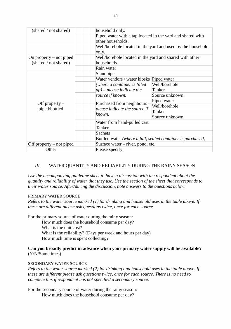
40

(shared / not shared) household only. Piped water with a tap located in the yard and shared with

other households.

On property – not piped

(shared / not shared)

Well/borehole located in the yard and used by the household only.

Well/borehole located in the yard and shared with other households.

Rain water

Off property – piped/bottled

Standpipe Water vendors / water kiosks

(where a container is filled up) – please indicate the source if known.

Piped water Well/borehole Tanker Source unknown Purchased from neighbours –

please indicate the source if known.

Piped water Well/borehole Tanker Source unknown Water from hand-pulled cart Tanker Sachets Bottled water (where a full, sealed container is purchased)

Off property – not piped Surface water – river, pond, etc. Other Please specify:

III. WATER QUANTITY AND RELIABILITY DURING THE RAINY SEASON

Use the accompanying guideline sheet to have a discussion with the respondent about the quantity and reliability of water that they use. Use the section of the sheet that corresponds to their water source. After/during the discussion, note answers to the questions below:

PRIMARY WATER SOURCE Refers to the water source marked (1) for drinking and household uses in the table above. If these are different please ask questions twice, once for each source.

For the primary source of water during the rainy season: How much does the household consume per day? What is the unit cost? What is the reliability? (Days per week and hours per day) How much time is spent collecting?

Can you broadly predict in advance when your primary water supply will be available? (Y/N/Sometimes)

SECONDARY WATER SOURCE Refers to the water source marked (2) for drinking and household uses in the table above. If these are different please ask questions twice, once for each source. There is no need to complete this if respondent has not specified a secondary source.

For the secondary source of water during the rainy season: How much does the household consume per day?

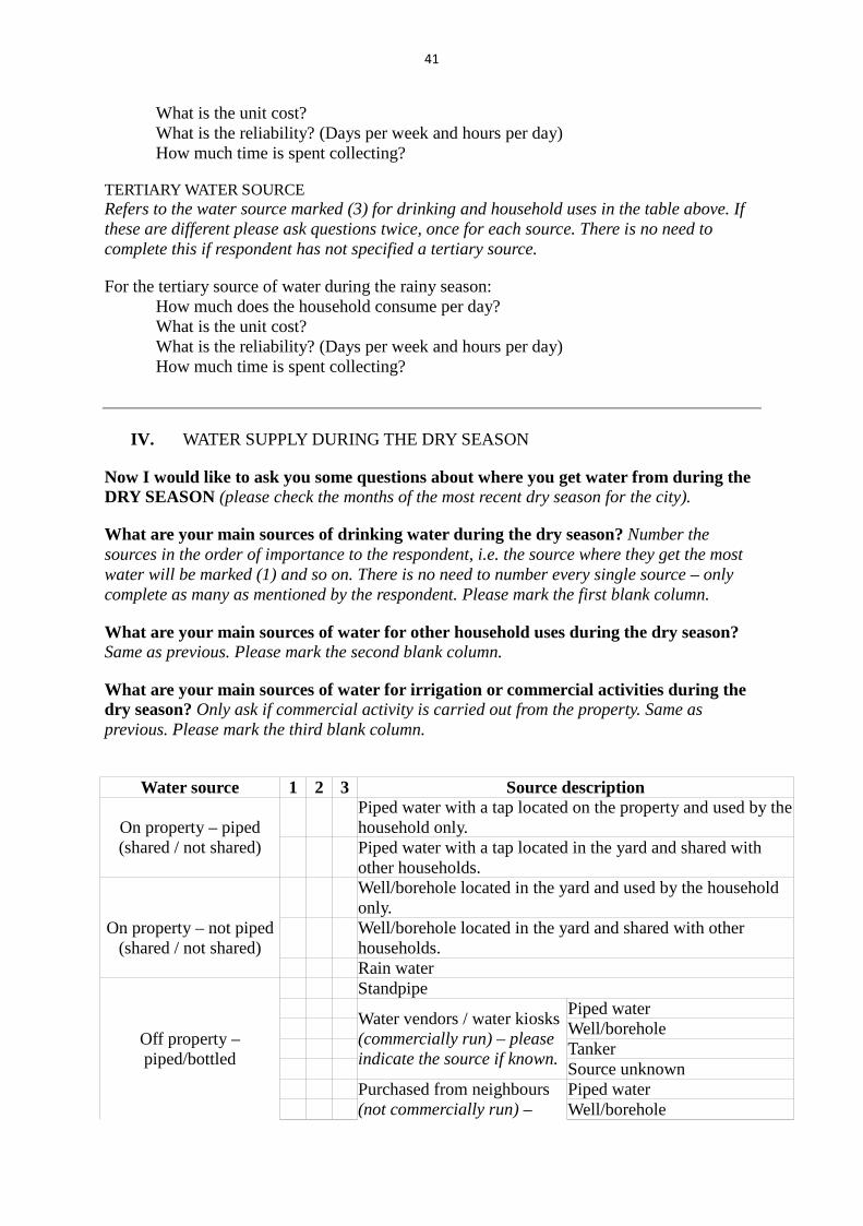
41

What is the unit cost? What is the reliability? (Days per week and hours per day) How much time is spent collecting?

TERTIARY WATER SOURCE Refers to the water source marked (3) for drinking and household uses in the table above. If these are different please ask questions twice, once for each source. There is no need to complete this if respondent has not specified a tertiary source.

For the tertiary source of water during the rainy season: How much does the household consume per day? What is the unit cost? What is the reliability? (Days per week and hours per day) How much time is spent collecting?

IV. WATER SUPPLY DURING THE DRY SEASON

Now I would like to ask you some questions about where you get water from during the DRY SEASON (please check the months of the most recent dry season for the city).

What are your main sources of drinking water during the dry season? Number the sources in the order of importance to the respondent, i.e. the source where they get the most water will be marked (1) and so on. There is no need to number every single source – only complete as many as mentioned by the respondent. Please mark the first blank column.

What are your main sources of water for other household uses during the dry season? Same as previous. Please mark the second blank column.

What are your main sources of water for irrigation or commercial activities during the dry season? Only ask if commercial activity is carried out from the property. Same as previous. Please mark the third blank column.

Water source 1 2 3 Source description

On property – piped (shared / not shared)

Piped water with a tap located on the property and used by the household only.

Piped water with a tap located in the yard and shared with other households.

On property – not piped

(shared / not shared)

Well/borehole located in the yard and used by the household only.

Well/borehole located in the yard and shared with other households.

Rain water

Off property – piped/bottled

Standpipe Water vendors / water kiosks

(commercially run) – please indicate the source if known.

Piped water Well/borehole Tanker Source unknown Purchased from neighbours

(not commercially run) – Piped water

Well/borehole

42

please indicate the source if known.

Tanker Source unknown Water from hand-pulled cart Tanker Sachets Bottled water (where a full, sealed container is purchased)

Off property – not piped Surface water – river, pond, etc. Other Please specify:

V. WATER QUANTITY AND RELIABILITY DURING THE DRY SEASON

Use the accompanying guideline sheet to have a discussion with the respondent about the quantity and reliability of water that they use. Use the section of the sheet that corresponds to their water source. After/during the discussion, note answers to the questions below:

PRIMARY WATER SOURCE Refers to the water source marked (1) for drinking and household uses in the table above. If these are different please ask questions twice, once for each source.

For the primary source of water during the dry season: How much does the household consume per day? What is the unit cost? What is the reliability? (Days per week and hours per day) How much time is spent collecting?

Could you broadly predict in advance when your primary water supply will be available? (Y/N/Sometimes)

SECONDARY WATER SOURCE Refers to the water source marked (2) for drinking and household uses in the table above. If these are different please ask questions twice, once for each source. There is no need to complete this if respondent has not specified a secondary source.

For the secondary source of water during the dry season: How much does the household consume per day? What is the unit cost? What is the reliability? (Days per week and hours per day) How much time is spent collecting?

TERTIARY WATER SOURCE Refers to the water source marked (3) for drinking and household uses in the table above. If these are different please ask questions twice, once for each source. There is no need to complete this if respondent has not specified a tertiary source.

For the tertiary source of water during the dry season: How much does the household consume per day? What is the unit cost? What is the reliability? (Days per week and hours per day) How much time is spent collecting?

43

VI. WATER STORAGE, HOUSING AND DISTANCE TO SOURCE

What is the total volume of water storage available within the property? Ask to be shown the available storage and make an estimate. Please specify units.

What is the total volume of water currently stored within the property? Ask to be shown the water stored and make an estimate. If this is not possible (e.g. if they are stored in the bedroom), ask the respondent to estimate the number of containers, indicate how big they are, and how full they are. Please specify units.

Who collects the water for the household? Note gender and age.

Observational notes on housing material: (Type of housing material to be used as proxy for income.) Add some observational notes about the number of rooms in the property and building materials for the walls, roof and floor. Note if the property has a toilet.

What is the distance to the primary source of water? Ask to be shown the primary source of water; this may be off the property and involve a short walk. Observe the distance to the source, functionality of the source, and price currently charged to check statements made by the respondent.

Thank the respondent for their time and reassure the confidentiality of their responses.

44

WATER QUANTITY AND RELIABILITY

Interviewer Guidelines These guidelines are to help interviewers establish the quantity of water that is used by each household. The methods for estimating quantity depend on the supply that the household uses, and therefore a discussion with the respondent should be conducted to extract all relevant information. The discussion will be very context-specific and relies on the discretion of the interviewer.

SACHETS/BOTTLED

Try to establish the volume of water contained in each bottle/sachet usually purchased. Try to establish how many bottles/sachets are purchased every day and every week. Try to establish the cost per bottle/sachet. Cross-check with approximate expenditure on water per week. (Cross-check with water usage within the household.)

CARRIED TO HOME FROM OUTSIDE COMPOUND (e.g. surface water, water vendors, kiosks.)

Try to establish the containers that are used to carry the water and estimate their size. Try to establish how many containers are filled/carried every day and every week. Try to establish the cost per filled container (or whatever volume is the common unit used – Nairobi usually uses 20 litres). Cross-check with approximate expenditure on water per week. (Cross-check with water usage within the household.) Try to establish how often water is available from their preferred source. Can they be sure of being able to fill a container every day? Does water only come every other day? Try to establish how many hours per day / days per week water is available (whichever is more appropriate).

CARRIED TO HOME FROM WITHIN COMPOUND (e.g. well, borehole or tap located within compound.)

Try to establish the containers that are used to carry the water and estimate their size. Try to establish how many containers are filled every day and every week. Household unlikely to be accurate on this. Check how they pay for this facility, and how much they pay. Is it included in rent? Cross-check with water usage within the household. Do this thoroughly as it is likely to be the best indicator. How much is usually used for cleaning/laundry/cooking? How often are these activities performed? Try to establish how often water is available from their preferred source. Can they be sure of being able to fill a container every day? Does water only come every other day? Try to establish how many hours per day / days per week water is available (whichever is more appropriate).

TAPS WITHIN THE HOME

Try to establish how much water the household stores and how they behave when they receive running water. Do they turn the taps on and fill up all their containers once a week? Once every couple of days? It couldn't hurt to examine water bills if there are any available, bearing in mind they may be inaccurate. Try to establish how often water is available from their tap. Can they be sure of being able to receive running water every day? Does water only come every other day? Try to establish how many hours per day / days per week water is available (whichever is more appropriate).

Check whether the household has a flush toilet in their house/compound. Where do they get water for flushing from?

45

Does the household own any of the following: (Please tick) Electricity Clock or watch Radio Television (black & white) Television (colour) Refrigerator Freezer Electric generator Solar panel Telephone (mobile Telephone (landline) Washing machine Camera (digital) Camera (non-digital) Personal Computer DVD/VCD player Sewing machine Bed Table Cupboard or cabinet What type of fuel does the household mainly use for cooking? (Please tick) Electricity LPG / natural gas Biogas Kerosene Coal/lignite Charcoal Wood Straw/shrubs/grass Agricultural crop Animal dung No food cooked in household Solar power Other (please describe)

Is cooking usually done in the house, a separate building, or outdoors?

Does the house have a separate room which is used as a kitchen? In the household, is food cooked on an open fire, an open stove or a closed stove? Please observe and record the main material of the floor: (Please tick) Earth/sand Dung Wood planks Palm/bamboo Parquet or polished wood Vinyl (PVC) or asphalt strips Ceramic tiles Cement Woollen or synthetic carpet Rubber carpet or linoleum Ceramic tiles Other (please describe)

Please observe and record the main material of the roof: (Please tick) Thatch or palm leaf Rustic mat Bamboo Wood planks Cardboard Metal/iron sheets Tin cans Calamine/cement fiber (asbestors) Ceramic tiles / brick tiles Cement Roofing shingles Asbestos / sheet roofing tiles Mud tiles Other (please describe)

WSUP Slum Water Supply Improvements Project INCOME INDICATORS

Taken from 2007 – 2008 DHS survey questionnaires for Kenya, Ghana and Zambia

46

Please observe and record the main material of the walls: (Please tick) Cane/palm/trunks Mud Bamboo with mud Stone with mud Plywood Cardboard Reused wood Cement Stone with lime/cement Bricks Cement blocks Covered adobe Wood planks / shingles How many rooms in this household are used for sleeping? Does the household own any of the following: (Please tick) Bicycle Motorcycle or motor scooter Animal-drawn cart Car or truck Boat with a motor Banana boat Does any member of this household own any agricultural land? If yes, how many acres / hectares / lima (Zambia only) / poles (Ghana only). Please specify units. Does any member of this household own any herds, livestock, other farm animals or poultry? Y/N

Please indicate the numbers of herds, livestock, farm animals or poultry owned by the household: (Please tick) Traditional/indigenous cattle Dairy cattle Beef cattle Horses, donkeys or mules Goats Sheep Pigs Rabbits Grasscutter (Greater Cane Rat) Chickens Other poultry (please specify)

Other (please specify

Does any member of this household have a bank account? Y/N

47

WSUP Slum Water Supply Improvements Project

PARTICIPANT INFORMATION SHEET

What is the purpose of the project?

This project is investigating how people access and use water in Nairobi. The end goal is to understand how demand for water would change if more people are connected to the network.

What are the possible benefits of taking part?

Whilst there is no immediate benefit from participation, it is hoped that your answers will contribute to improving water supply for everyone in Nairobi.

Can I withdraw my answers at a later date?

You can withdraw at any time during the interview or at a later date by contacting the lead researcher at the email address below. You do not need to give a reason to withdraw. Your responses will be anonymous and you will never be identifiable in any data sets, reports or publications.

Who is funding and carrying out the research?

This research is funded by Water and Sanitation for Urban Poor – a non-profit partnership aimed at improving water and sanitation in urban areas. The research is being carried out by the University of Leeds.

Contact for further information:

Dr Dabo Guan Senior Lecturer: Environmental Economics & Governance School of Earth and Environment University of Leeds, LS2 9JT, Leeds, UK Phone: +44(0) 113 34 37432 Email: d.guan@leeds.ac.uk

48

APPENDIX 2: VARIABLES COLLECTED

Variable Full Name Description Units / Input Format

Q_ID Questionnaire ID Questionnaire ID number. first 3 letters of city name followed by a number.

Interview_date Interview date Date on which the interview took place.

day/month/year

City City City in which the interview took place.

text

Location Location Location in which the interview took place. NB - whilst not all cities may use locations/sub-locations, it would be useful for the purpose of this project to assign two levels of neighbourhood identification within the city, regardless of whatever administrative boundaries are used in reality.

text

Sub-location Sub-location Sub-location in which the interview took place.

text

Interviewer Interviewer name Name of the person who conducted the interview.

text

Gender Gender Gender of respondent. m or f Age_cat Age category Age band category which the

respondent falls into. 1 = (18-30), 2 = (31-40), 3 = (41-50), 4 = (51-60), 5 = (61-70), 6 = (71-80), 7 = (80+).

category number

HH_head Household head? Binary variable indicating whether the respondent is the household head. 0 = NO, 1 = YES.

0 or 1

No_ppl Number of people The number of people living within the household.

number of people

No_infants Number of infants The number of infants living within the household.

number of infants

No_children Number of children The number of children living within the household.

number of children

Commercial Commercial? Binary variable indicating whether any commercial activity is carried out from the property. 0 = NO, 1 = YES.

0 or 1

Educ_cat Education category Highest education category achieved by any member of the household.

category number

Tenure_status Tenure status Tenure status category for the household.

category number

Length_resid Length of residence Length of time that the household has been resident in the property.

years

Rainy_drinking_1 Rainy season, primary drinking source category

Category of primary drinking water source used in the rainy season.

category number

Rainy_drinking_2 Rainy season, secondary drinking source category

Category of secondary drinking water source used in the rainy

category number

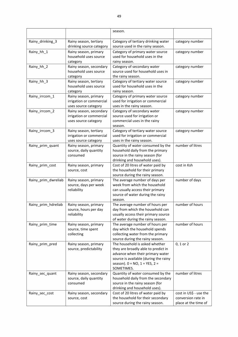
49

season.

Rainy_drinking_3 Rainy season, tertiary drinking source category

Category of tertiary drinking water source used in the rainy season.

category number

Rainy_hh_1 Rainy season, primary household uses source category

Category of primary water source used for household uses in the rainy season.

category number

Rainy_hh_2 Rainy season, secondary household uses source category

Category of secondary water source used for household uses in the rainy season.

category number

Rainy_hh_3 Rainy season, tertiary household uses source category

Category of tertiary water source used for household uses in the rainy season.

category number

Rainy_irrcom_1 Rainy season, primary irrigation or commercial uses source category

Category of primary water source used for irrigation or commercial uses in the rainy season.

category number

Rainy_irrcom_2 Rainy season, secondary irrigation or commercial uses source category

Category of secondary water source used for irrigation or commercial uses in the rainy season.

category number

Rainy_irrcom_3 Rainy season, tertiary irrigation or commercial uses source category

Category of tertiary water source used for irrigation or commercial uses in the rainy season.

category number

Rainy_prim_quant Rainy season, primary source, daily quantity consumed

Quantity of water consumed by the household daily from the primary source in the rainy season (for drinking and household uses).

number of litres

Rainy_prim_cost Rainy season, primary source, cost

Cost of 20 litres of water paid by the household for their primary source during the rainy season.

cost in Ksh

Rainy_prim_dwreliab Rainy season, primary source, days per week reliability

The average number of days per week from which the household can usually access their primary source of water during the rainy season.

number of days

Rainy_prim_hdreliab Rainy season, primary source, hours per day reliability

The average number of hours per day from which the household can usually access their primary source of water during the rainy season.

number of hours

Rainy_prim_time Rainy season, primary source, time spent collecting

The average number of hours per day which the household spends collecting water from the primary source during the rainy season.

number of hours

Rainy_prim_pred Rainy season, primary source, predictability

The household is asked whether they are broadly able to predict in advance when their primary water source is available (during the rainy season). 0 = NO, 1 = YES, 2 = SOMETIMES.

0, 1 or 2

Rainy_sec_quant Rainy season, secondary source, daily quantity consumed

Quantity of water consumed by the household daily from the secondary source in the rainy season (for drinking and household uses).

number of litres

Rainy_sec_cost Rainy season, secondary source, cost

Cost of 20 litres of water paid by the household for their secondary source during the rainy season.

cost in US$ - use the conversion rate in place at the time of

50

the survey.

Rainy_sec_dwreliab Rainy season, secondary source, days per week reliability

The average number of days per week from which the household can usually access their secondary source of water during the rainy season.

number of days

Rainy_sec_hdreliab Rainy season, secondary source, hours per day reliability

The average number of hours per day from which the household can usually access their secondary source of water during the rainy season.

number of hours

Rainy_sec_time Rainy season, secondary source, time spent collecting

The average number of hours per day which the household spends collecting water from the secondary source during the rainy season.

number of hours

Rainy_sec_pred Rainy season, secondary source, predictability

The household is asked whether they are broadly able to predict in advance when their secondary water source is available (during the rainy season). 0 = NO, 1 = YES, 2 = SOMETIMES.

0, 1 or 2

Rainy_tert_quant Rainy season, tertiary source, daily quantity consumed

Quantity of water consumed by the household daily from the tertiary source in the rainy season (for drinking and household uses).

number of litres

Rainy_tert_cost Rainy season, tertiary source, cost

Cost of 20 litres of water paid by the household for their tertiary source during the rainy season.

cost in US$ - use the conversion rate in place at the time of the survey.

Rainy_tert_dwreliab Rainy season, tertiary source, days per week reliability

The average number of days per week from which the household can usually access their tertiary source of water during the rainy season.

number of days

Rainy_tert_hdreliab Rainy season, tertiary source, hours per day reliability

The average number of hours per day from which the household can usually access their tertiary source of water during the rainy season.

number of hours

Rainy_tert_time Rainy season, tertiary source, time spent collecting

The average number of hours per day which the household spends collecting water from the tertiary source during the rainy season.

number of hours

Rainy_tert_pred Rainy season, tertiary source, predictability

The household is asked whether they are broadly able to predict in advance when their tertiary water source is available (during the rainy season). 0 = NO, 1 = YES, 2 = SOMETIMES.

0, 1 or 2

Dry_drinking_1 Dry season, primary drinking source category

Category of primary drinking water source used in the dry season.

category number

Dry_drinking_2 Dry season, secondary drinking source category

Category of secondary drinking water source used in the dry season.

category number

51

Dry_drinking_3 Dry season, tertiary drinking source category

Category of tertiary drinking water source used in the dry season.

category number

Dry_hh_1 Dry season, primary household uses source category

Category of primary water source used for household uses in the dry season.

category number

Dry_hh_2 Dry season, secondary household uses source category

Category of secondary water source used for household uses in the dry season.

category number

Dry_hh_3 Dry season, tertiary household uses source category

Category of tertiary water source used for household uses in the dry season.

category number

Dry_irrcom_1 Dry season, primary irrigation or commercial uses source category

Category of primary water source used for irrigation or commercial uses in the dry season.

category number

Dry_irrcom_2 Dry season, secondary irrigation or commercial uses source category

Category of secondary water source used for irrigation or commercial uses in the dry season.

category number

Dry_irrcom_3 Dry season, tertiary irrigation or commercial uses source category

Category of tertiary water source used for irrigation or commercial uses in the dry season.

category number

Dry_prim_quant Dry season, primary source, daily quantity consumed

Quantity of water consumed by the household daily from the primary source in the dry season (for drinking and household uses).

number of litres

Dry_prim_cost Dry season, primary source, cost

Cost of 20 litres of water paid by the household for their primary source during the dry season.

cost in Ksh

Dry_prim_dwreliab Dry season, primary source, days per week reliability

The average number of days per week from which the household can usually access their primary source of water during the dry season.

number of days

Dry_prim_hdreliab Dry season, primary source, hours per day reliability

The average number of hours per day from which the household can usually access their primary source of water during the dry season.

number of hours

Dry_prim_time Dry season, primary source, time spent collecting

The average number of hours per day which the household spends collecting water from the primary source during the dry season.

number of hours

Dry_prim_pred Dry season, primary source, predictability

The household is asked whether they are broadly able to predict in advance when their primary water source is available (during the dry season). 0 = NO, 1 = YES, 2 = SOMETIMES.

0, 1 or 2

Dry_sec_quant Dry season, secondary source, daily quantity consumed

Quantity of water consumed by the household daily from the secondary source in the dry season (for drinking and household uses).

number of litres

Dry_sec_cost Dry season, secondary source, cost

Cost of 20 litres of water paid by the household for their secondary source during the dry season.

cost in Ksh

Dry_sec_dwreliab Dry season, secondary source, days per week reliability

The average number of days per week from which the household can usually access their secondary

number of days

52

source of water during the dry season.

Dry_sec_hdreliab Dry season, secondary source, hours per day reliability

The average number of hours per day from which the household can usually access their secondary source of water during the dry season.

number of hours

Dry_sec_time Dry season, secondary source, time spent collecting

The average number of hours per day which the household spends collecting water from the secondary source during the dry season.

number of hours

Dry_sec_pred Dry season, secondary source, predictability

The household is asked whether they are broadly able to predict in advance when their secondary water source is available (during the dry season). 0 = NO, 1 = YES, 2 = SOMETIMES.

0, 1 or 2

Dry_tert_quant Dry season, tertiary source, daily quantity consumed

Quantity of water consumed by the household daily from the tertiary source in the dry season (for drinking and household uses).

number of litres

Dry_tert_cost Dry season, tertiary source, cost

Cost of 20 litres of water paid by the household for their tertiary source during the dry season.

cost in Ksh

Dry_tert_dwreliab Dry season, tertiary source, days per week reliability

The average number of days per week from which the household can usually access their tertiary source of water during the dry season.

number of days

Dry_tert_hdreliab Dry season, tertiary source, hours per day reliability

The average number of hours per day from which the household can usually access their tertiary source of water during the dry season.

number of hours

Dry_tert_time Dry season, tertiary source, time spent collecting

The average number of hours per day which the household spends collecting water from the tertiary source during the dry season.

number of hours

Dry_tert_pred Dry season, tertiary source, predictability

The household is asked whether they are broadly able to predict in advance when their tertiary water source is available (during the dry season). 0 = NO, 1 = YES, 2 = SOMETIMES.

0, 1 or 2

Vol_stored_avail Volume of storage available

The number of litres of storage capacity available within containers owned by the household.

number of litres

Vol_stored_curr Volume of storage currently used

The number of litres of water which were being stored by the household at the time of the interview.

number of litres

Collects_gender Collection gender The gender of the person who most commonly collects water in the household.

m or f

53

Collects_agecat Collection age category The age category of the person who most commonly collects water in the household.

category number

Toilet Toilet? Binary variable indicating whether the household has a toilet. 0 = NO, 1 = YES.

0 or 1

Dist Distance from source Distance between the household and the primary source, in metres.

number of metres

Flag Flag? Binary variable indicating whether there is anything about the household that might cause the researcher to suspect it might be an outlier in any way, or if very large estimates were made. Put a 1 here if, for instance, it was impossible to estimate the total storage volume, or if the household conducts commercial activity from the property that consumes an extremely large amount of water. Otherwise, put 0.

0 or 1

Variable Full name Category Number

Value

Age_cat

Age category

1 18-30

2 31-40 3 41-50 4 51-60 5 61-70 6 71-80 7 80+

Educ_cat

Education category

1 No formal education

2 Competed primary education 3 Completed secondary education 4 Competed post-secondary training 5 Completed university 6 Other

Tenure_status

Tenure status

1 Household owns the property.

2 Household rents the property. 3 Household rents a room in the property.

Water category related variables

Water source category

1 Piped water with a tap located on the property and used by the household only.

2 Piped water with a tap located in the yard and shared with other households.

3 Well/borehole located in the yard and used by the household only.

4 Well/borehole located in the yard and shared with other households.

5 Rain water 6 Standpipe

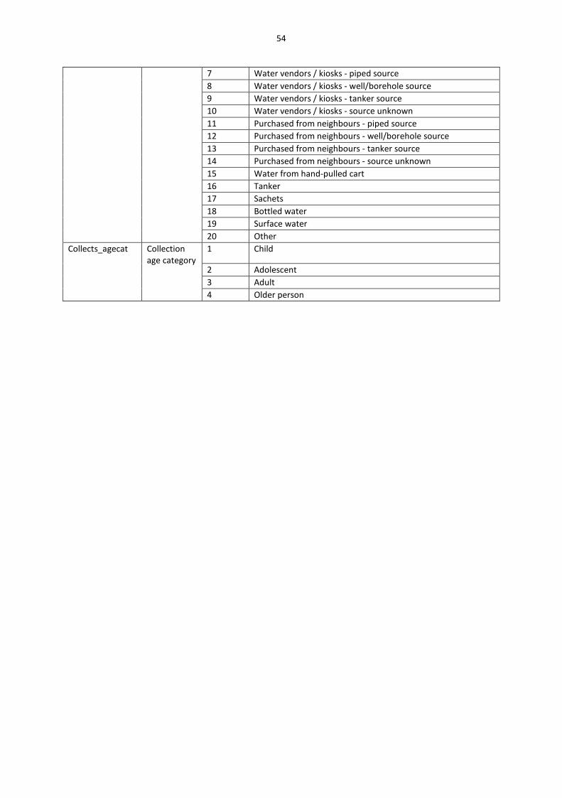
54

7 Water vendors / kiosks - piped source 8 Water vendors / kiosks - well/borehole source 9 Water vendors / kiosks - tanker source 10 Water vendors / kiosks - source unknown 11 Purchased from neighbours - piped source 12 Purchased from neighbours - well/borehole source 13 Purchased from neighbours - tanker source 14 Purchased from neighbours - source unknown 15 Water from hand-pulled cart 16 Tanker 17 Sachets 18 Bottled water 19 Surface water 20 Other

Collects_agecat

Collection age category

1 Child

2 Adolescent 3 Adult 4 Older person

55

APPENDIX 3: FACTOR ANALYSIS - SUPPORTING DATA Supporting information for the PCA carried out in Section 4.5 is given below.

Rotated Component Matrixa

Component

1 2 3 4

Neighbourhood Category .810 -.065 .152 -.130

Wealth Category - ordered .758 -.234 .286 -.283

Water Source New Category .705 -.448 .092 -.249

Household vends water -.687 .037 .318 -.261

Water is included in rent .182 -.821 -.207 -.017

Cost of 20 litres of water -.038 .756 -.039 .288

Reliability in days per week -.161 .707 -.005 -.303

Age Category -.059 .012 .730 .192

Household owns property -.069 .067 .696 -.060

Available volume of storage on property

.178 -.023 .566 -.261

Number of people in the household

.246 .052 .417 .067

Time to collect in minutes -.051 -.170 .024 .824

Distance to source in metres -.148 .249 .000 .737

Extraction Method: Principal Component Analysis.

Rotation Method: Varimax with Kaiser Normalization.a

a. Rotation converged in 5 iterations.

KMO and Bartlett's Test

Kaiser-Meyer-Olkin Measure of Sampling Adequacy. .679

Bartlett's Test of Sphericity Approx. Chi-Square 349.037

df 78

Sig. .000

56