HAL Id: ird-00543818http://hal.ird.fr/ird-00543818

Submitted on 6 Dec 2010

HAL is a multi-disciplinary open accessarchive for the deposit and dissemination of sci-entific research documents, whether they are pub-lished or not. The documents may come fromteaching and research institutions in France orabroad, or from public or private research centers.

L’archive ouverte pluridisciplinaire HAL, estdestinée au dépôt et à la diffusion de documentsscientifiques de niveau recherche, publiés ou non,émanant des établissements d’enseignement et derecherche français ou étrangers, des laboratoirespublics ou privés.

Downscaling MODIS-derived maps using GIS boostedregression trees : the case of frost occurrence over the

arid Andean highlands of BoliviaRobin Pouteau, Serge Rambal, Jean-Pierre Ratte, Fabien Gogé, Richard

Joffre, Thierry Winkel

To cite this version:Robin Pouteau, Serge Rambal, Jean-Pierre Ratte, Fabien Gogé, Richard Joffre, et al.. DownscalingMODIS-derived maps using GIS boosted regression trees : the case of frost occurrence over the aridAndean highlands of Bolivia. Remote Sensing of Environment, Elsevier, 2011, 115 (1), pp.117-129.<10.1016/j.rse.2010.08.011>. <ird-00543818>

1

Downscaling MODIS-derived maps using GIS and boosted regression trees: 1

the case of frost occurrence over the arid Andean highlands of Bolivia 2

3

Pouteau R., Rambal S., Ratte J.P., Gogé F., Joffre R., Winkel T. 4

5

6

Authors' addresses and affiliations 7

Robin Pouteau (a, b), Serge Rambal (b), Jean-Pierre Ratte (b), Fabien Gogé (b), Richard Joffre (a, b), 8

Thierry Winkel (a) 9

(a) IRD, CEFE-CNRS, F-34293 Montpellier cedex 5, France 10

(b) UMR 5175, CEFE-CNRS, F-34293 Montpellier cedex 5, France 11

12

Corresponding author 13

Thierry Winkel 14

IRD, CEFE-CNRS, F-34293 Montpellier cedex 5, France 15

E-mail: thierry.winkel@ird.fr 16

17

Citation 18

Pouteau R., Rambal S., Ratte J.P., Gogé F., Joffre R., Winkel T. 2011. Downscaling MODIS-derived 19

maps using GIS and boosted regression trees: the case of frost occurrence over the arid Andean 20

highlands of Bolivia. Remote Sensing of Environment, 115 (1): 117-129. 21

DOI: 0.1016/j.rse.2010.08.011 22

23

2

Abstract 24

Frost risk assessment is of critical importance in tropical highlands like the Andes where human 25

activities thrives at altitudes up to 4200 m, and night frost may occur all the year round. In these semi-26

arid and cold regions with sparse meteorological networks, remote sensing and topographic modeling 27

are of potential interest for understanding how physiography influences the local climate regime. After 28

integrating night land surface temperature from the MODIS satellite, and physiographic descriptors 29

derived from a digital elevation model, we explored how regional and landscape-scale features 30

influence frost occurrence in the southern altiplano of Bolivia. Based on the high correlation between 31

night land surface temperature and minimum air temperature, frost occurrence in early-, middle- and 32

late-summer periods were calculated from satellite observations and mapped at a 1-km resolution over 33

a 45000 km² area. Physiographic modeling of frost occurrence was then conducted comparing multiple 34

regression (MR) and boosted regression trees (BRT). Physiographic predictors were latitude, elevation, 35

distance from salt lakes, slope steepness, potential insolation, and topographic convergence. Insolation 36

influence on night frost was tested assuming that ground surface warming in the daytime reduces frost 37

occurrence in the next night. Depending on the time period and the calibration domain, BRT models 38

explained 74% to 90% of frost occurrence variation, outperforming the MR method. Inverted BRT 39

models allowed the downscaling of frost occurrence maps at 100-m resolution, illustrating local 40

processes like cold air drainage. Minimum temperature lapse rates showed seasonal variation and 41

mean values higher than those reported for temperate mountains. When applied at regional and 42

subregional scales successively, BRT models revealed prominent effects of elevation, latitude and 43

distance to salt lakes at large scales, whereas slope, topographic convergence and insolation gained 44

influence at local scales. Our results highlight the role of daytime insolation on night frost occurrence at 45

local scale, particularly in the early- and mid-summer periods when solar astronomic forcing is 46

maximum. Seasonal variations and interactions in physiographic effects are also shown. Nested effects 47

of physiographic factors across scales are discussed, as well as potential applications of physiographic 48

modeling to downscale ecological processes in complex terrains. 49

50

Key words 51

altiplano; Andes; Bolivia; boosted regression trees; DEM; downscaling; frost risk mapping; MODIS; 52

physiography; temperature lapse rate; topoclimate model; satellite land surface temperature; seasonal 53

variation; spatial variation 54

55

56

3

1. Introduction 57

Low air temperature is one of the most important factors controlling vegetation zonation and key 58

processes such as evapotranspiration, carbon fixation and decomposition, plant productivity and 59

mortality in natural and cultivated mountain ecosystems (Chen et al., 1999; Nagy et al., 2003). 60

Depending on vegetation structure, landscape position or soil properties, frost can damage plant tissues 61

thus affecting forest, pasture and crop productivity (Blennow & Lindkvist, 2000). These damages have 62

consequences for human populations, particularly in the tropics where highlands often remain densely 63

populated (Grötzbach & Stadel, 1997). In the Andes of Argentina, Bolivia, Chile, Ecuador and Peru 64

agriculture thrives at altitudes up to 4200 m (Del Castillo et al., 2008) and treeline reaches its world's 65

highest elevation up to 5100 m (Hoch & Körner, 2005) in spite of night frost occurring on more than 300 66

days practically spread all over the year (Garcia et al., 2007; Gonzalez et al., 2007; Rada et al., 2009; 67

Troll, 1968). In the southern Andes, sparsely vegetated areas juxtaposing extended flat plains around 68

salt lakes and steep slopes on the cordilleras and volcanos, display semi-arid and desert landscapes 69

largely dominated by terrain structure. Subjected to the night/day and sunlit/shaded slope contrasts 70

characteristic of the mountain climate, this environment is well suited for examining the influence of 71

regional and landscape-scale physiography on the local climate regime, and particularly frost 72

occurrence. 73

Several studies on topoclimate in highlands showed that elevation and slope are the main 74

explanatory variables in modeling local climate spatial variability (Chuanyan et al., 2005). By means of 75

digital elevation models and astronomical equations, the potential insolation (incoming solar radiation) 76

has been included as an additional independant variable in some of these models, substantially 77

improving their capacity to predict free-air as well as soil-surface temperature distributions (Benavides 78

et al., 2007; Blennow & Lindkvist ,2000; Fridley 2009; Fu & Rich, 2002). Among the physiographic 79

variables, elevation and slope steepness are known to influence cold air drainage at night and, hence, 80

the distribution of frost risks at landscape scale (Lundquist et al., 2008; Pypker et al., 2007a). In the 81

daytime, slope aspect and physiographic shading effects control the effective radiation load per unit of 82

soil areas, resulting in very contrasted values of daily maximum soil temperature (Fu & Rich, 2002). 83

Minimum night temperature might be sensitive to insolation during the previous day, since soil surface 84

warming during that day could dampen soil radiative cooling in the next night. Though challenged by 85

studies on minimum air temperature variations in moderately high mountains under temperate climate 86

(Blennow 1998; Dobrowski et al., 2009), this hypothesis should be tested in the central part of the 87

Andes, where low latitude, high elevation (typically ranging between 3600 and 4200 m) and sparse 88

vegetation result in much greater radiation load and thermal contrasts across shaded and sunlit areas. 89

Besides, using a downscaling approach, Fridley (2009) noticed that the lack of relationship between 90

daytime radiation and nighttime temperature is true at local scale lower than 1000 m but not at regional 91

scale (Great Smoky Mountains, USA), where variations in radiation balance across locations do 92

influence nighttime temperature distribution particularly in cooler situations. Considering the Andes, 93

recent work by Bader & Ruijten (2008) and Bader et al. (2008) used topographic modeling and remote 94

sensing data to examine the response of vegetation distribution to climate warming, but we should go 95

back to Santibañez et al. (1997) and François et al. (1999) to find studies on the links between frost 96

4

climatology and physiography over this region. These early works were not continued, and the case of 97

the Andean highlands remained poorly documented in spite of the potential interest of that region, 98

densely populated and representative of the tropical mountains vulnerable to global warming (Vuille et 99

al., 2008). 100

Analyzing topographic effects on free-air or land surface temperature also led to reevaluate the 101

simplifying assumption of a generic environmental lapse rate (the decrease in free-air temperature as 102

elevation rises, typically assumed to be -0.6 °C per 100 m), commonly applied in hydrological and 103

ecological studies to extrapolate air temperature in mountain areas. In fact, several studies show 104

temperature lapse rate variations due to seasonality, height above the ground, or ground surface 105

characteristics (Blandford et al., 2008; Dobrowski et al., 2009; Fridley 2009; Lookingbill & Urban, 2003; 106

Marshall et al., 2007), though no detailed reports were published for the Central Andes. 107

Most of the above mentionned studies used multiple linear regression for modeling the influence of 108

physiography on free-air or soil-surface temperatures. The present study resorts to an advanced form of 109

regression, the boosted regression trees (BRT). BRT use the boosting technique to combine large 110

numbers of relatively simple tree models to optimize predictive performance. BRT have been used 111

successfully in human biology (Friedman and Meulman 2003), land cover mapping (Lawrence et al., 112

2004), biogeography (Parisien & Moritz, 2009), species distribution (Elith et al., 2008), and soil science 113

(Martin et al., 2009). They offer substantial advantages over classical regression models since they 114

handle both qualitative and quantitative variables, can accomodate missing data and correlated 115

predictive variables, are relatively insensitive to outliers and to the inclusion of irrelevant predictor 116

variables, and are able to model complex interactions between predictors (Elith et al., 2008; Martin et 117

al., 2009). Though direct graphic representation of the complete tree model is impossible with BRT, the 118

model interpretation is made easy by identifying the variables most relevant for prediction, and then 119

visualizing the partial effect of each predictor variable after accounting for the average effect of the 120

other variables (Friedman & Meulman, 2003). 121

The aims of the present work were: i) to explore how regional and landscape-scale physiography 122

influence frost occurrence in Andean highlands through integration of field and remote sensing data, 123

digital terrain analysis, and GIS, ii) to downscale regional frost occurrence maps at a level relevant for 124

farming and land management decisions using BRT models. This study was focused on the austral 125

summer period, from November to April, when frost holds the greatest potential impact for local farming 126

activities. 127

2. Material and methods 128

2.1. Study area and regional climate 129

The study area was located at the southwest of the Bolivian highlands, near the borders of 130

Argentina and Chile, between 19°15’ and 22°00’ South and between 66°26’ and 68°15’ West. This 131

region, boarded by the western Andes cordillera, is characterized by the presence in its centre of a 132

ca.100 x 100 km dry salt expanse, the Salar of Uyuni, while another salt lake, the Salar of Coipasa, lies 133

at the north of the study area. The landscapes show a mosaic of three types of land units: more or less 134

extended flat shores surrounding the salt lakes (elevation ca. 3650 m) and an alternation of valleys and 135

5

volcanic relieves (culminating at 6051 m) in the hinterland. The native vegetation of this tropical Andean 136

ecosystem, also known as puna, consists of a mountain steppe of herbaceous and shrub species (e.g. 137

Baccharis incarum, Parastrephia lepidophylla, and Stipa spp.) (Navarro & Ferreira, 2007) traditionally 138

used as pastures but progressively encroached by the recent and rapid expansion of quinoa crop 139

(Chenopodium quinoa Willd.) (Vassas et al., 2008). 140

Due to its low latitude and high elevation, the study area is characterized by a cold and arid tropical 141

climate. Average precipitations vary between 100 and 350 mm year-1 from the South to the North of the 142

region (Geerts et al., 2006), presenting an unimodal distribution with a dry season from April to October. 143

The annual average temperature (close to 9 °C) hides daily thermal amplitudes higher than seasonal 144

amplitudes, of up to 25 °C (Frère et al., 1978). These particular thermal conditions lead to high frost 145

risks throughout the year. Advections of air masses from the South Pole represent only 20% of the 146

observed frosty nights (Frère et al., 1978) and are four times less frequent in the summer than during 147

the winter, when the intertropical convergence zone goes northward (Ronchail, 1989). Therefore, the 148

main climatic threat lies in radiative frost, occurring during clear and calm nights. As reported by local 149

peasants, frost occurence shows a strong topographical and orographical dependence, as well as a 150

marked seasonality. This seasonality lead us to split the active vegetation period into three time periods 151

characterizing the mean regional climate dynamics in the summer rainy season: November-December 152

when precipitation and minimum temperature rise progressively, January-February when precipitation 153

and temperature are at their maximum, and March-April when both begin to decrease. 154

2.2. Data 155

2.2.1. Meteorological ground data 156

In the study area, daily air temperature records were available in three meteorological stations: one 157

at Salinas de Garci Mendoza (19°38’S, 67°40’W) managed by the SENAMHI (Meteorology and 158

Hydrology National Service, Bolivia) where daily minimum air temperature (Tn) was recorded in 1989 159

and from 1998 to 2006, and two others at Irpani (19°45’S, 67°41’W) and Jirira (19°51’S, 67°34’W) 160

where meteorological stations set up by the IRD (Research Institute for Development, France) recorded 161

semi-hourly air temperature from 23 November 2005 to 18 February 2006 in Irpani, and from 6 162

November 2006 to 31 December 2007 in Jirira. This dataset was temporally and spatially insufficient to 163

interpolate frost risks at a regional scale, but it allowed to establish the relationship between air 164

temperature and remotely sensed land surface temperature. 165

2.2.2. Remotely sensed data 166

The two sensors, Terra and Aqua, of the satellite system MODIS give daily images of the Earth 167

radiative land surface temperature. Images from the fifth version of the MYD11A1 MODIS product were 168

concatenated and projected in the UTM-19S (Universal Transverse Mercator 19 South) coordinate 169

system using the MODIS projection tool. In this way, daily 1-km resolution images of the radiative land 170

surface temperature (Ts) over the study area were obtained. Ts images recorded by the Aqua sensor 171

around 2 a.m. were used as they were closer to the Tn data recorded at ground level and closer to the 172

true physiological conditions experienced by the vegetation (François et al., 1999). Time series of 173

nominal 1-km spatial resolution MODIS data were downloaded from NASA's EOS data gateway 174

6

(https://wist.echo.nasa.gov/) from 20 July 2001 to 25 April 2006 and from 01 January 2007 to 31 175

December 2007. Due to the particular surface properties of the salt lakes of Coipasa and Uyuni in terms 176

of surface moisture and radiative emissivity, parameter estimations were considered dubious there and 177

Ts data for the salt lakes were discarded from the analysis. This database was managed and analyzed 178

using the ENVI 4.2. software (ITT Visual Information Solutions, www.ittvis.com). The statistical 179

correspondence between Tn data recorded in the meteorological stations of Salinas, Irpani and Jirira 180

and Ts data of the pixels including these three localities was examined by linear regression and 181

Pearson correlation. 182

Apart from Ts measurements during clear nights, MODIS images also bring information about the 183

possible presence of clouds between the Earth surface and the satellite at the time of the record. The 184

information of these “flagged” images is valuable for our purpose since radiative frost would not occur 185

during cloudy nights. The frequency of cloudy pixels in the daily MODIS images was thus calculated 186

and used in the frost occurrence calculation (see below). 187

2.2.3. Digital elevation model and physiographic predictors 188

The SRTM digital elevation model (Farr et al., 2007) with a 90 m horizontal resolution and a 189

vertical accuracy better than 9 m was used after resampling to 100 m to make easier the 190

correspondence between the digital elevation model and the MODIS images at 1-km scale. In a GIS 191

environment using Idrisi Kilimanjaro, Envi 4.2. and ArcMap 9.2. softwares, eight physiographic variables 192

were calculated at a 100-m resolution for each location to examine their potential role in the spatial 193

determinism of frost and to downscale frost maps to levels closer to those of frost impacts on anthropic 194

activities (Table 1). The compound topographic index (CTI) was used as an index of cold air drainage 195

(Gessler et al., 2000), with low CTI values representing convex positions like moutain crests and with 196

high CTI values representing concave positions like coves or hillslope bases. Three insolation variables 197

(DPI, MPI and API) were calculated by the ArcMap 9.2. solar analysis tool. They express the amount of 198

radiative energy received across all wavelengths over the course of a typical seasonal day (DPI), or 199

from sunrise to 12:00 (MPI), or from 12:00 to sunset (API) of such a day. 200

These insolation variables account for site latitude and elevation, slope steepness and aspect, 201

daily and seasonal sun angle, and shadows cast by surrounding heights. API was calculated to 202

examine the specific influence of insolation in the afternoon just before the considered night, with the 203

hypothesis that high soil surface insolation and warming would affect the soil energy balance, and thus 204

reduce the risk of radiative frost in the following night (without regards to other potential factors such as 205

soil albedo, soil water content, air humidity, etc. see Garcia et al. (2004)). Similarly, MPI was calculated 206

as a surrogate to the early morning insolation, with the hypothesis that areas in the shade of 207

surrounding heights in the early morning would experience cooler conditions for a longer time, thus 208

being more vulnerable to frost than sunlit areas. In the calibration procedure, these 100-m resolution 209

variables were upscaled at 1-km resolution by averaging 10 x 10 pixel clusters in the DEM 100-m 210

images, thus fitting the 1-km resolution of the remotely sensed frost occurrence maps. 211

212

213

7

Table 1. Ranges of physiographic variables observed over the study area. 214

Variable Minimum Maximum Unit

LAT latitude in UTM 19 South -22.00 -19.24 decimal degree

ELE elevation 3540 6051 m

SLO slope steepness 0 35 degree

DPI daily potential insolation

Nov-Dec 6900 9075 W m-²

Jan-Feb 7040 8935 W m-²

Mar-Apr 4604 7897 W m-²

MPI morning potential insolation

Nov-Dec 510 1861 W m-²

Jan-Feb 466 1772 W m-²

Mar-Apr 264 1240 W m-²

API afternoon potential insolation

Nov-Dec 2819 5075 W m-²

Jan-Feb 2816 5000 W m-²

Mar-Apr 2079 4308 W m-²

LDS distance from salt lakes 0 5.04 Ln (km + 1)

CTI compound topographic index 5.7 14.1 -

215

2.3. Physiographic modeling of frost occurrence over regional and subregional domains 216

2.3.1. MODIS-derived frost occurrence 217

Frost is detected by remote sensing when surface temperature appears negative on cloudfree 218

images. Based on the standard meteorological threshold of 0 °C, frost occurrence (R) for a specific time 219

period was therefore defined as follows: 220

221

R = Prob (Ts < 0 °C) * F (1) 222

223

where: R = frost occurrence at the 0 °C threshold (relative probability ranging from 0 to 1), Prob (Ts < 0 224

°C) = probability of the surface radiative temperature being lower than 0°C, F = frequency of cloudless 225

days in the considered period. Note that “frost occurrence” is used here instead of frost risk to 226

differentiate our estimates based on 6-year daily Ts values from climatological estimates based on 227

longer data series. 228

In order to calculate the probability Prob (Ts < 0 °C) , the distribution of the random variable Ts 229

during successive time periods (namely: November-December, January-February, March-April) was 230

studied, checking its normality through the Kolmogorov-Smirnov test. For each 1-km pixel and each 231

time period, Ts mean and standard deviation, cloudless day frequency (F) and, finally, frost occurrence 232

8

(R) were calculated from the available nighttime remotely sensed data series (n = 366 , 355, and 361 in 233

the ND, JF and MA periods respectively). Maps of observed (remotely sensed) frost occurrence at 1-km 234

resolution were then generated by applying Eq. (1) for each time period. 235

2.3.2. Frost occurrence models over regional and subregional domains 236

A subsample of 1-km pixels (n = 7500) was randomly selected for the calibration of the 237

physiography-frost occurrence relationships over the entire study area (hereafter called "regional 238

models"). Regional BRT were built for each seasonal period (November-December, January-February, 239

March-April) using the gbm package version 1.6-3 developped under R software (R Development Core 240

Team 2006). A bag fraction of 0.5 was used which means that, at each step of the boosting procedure, 241

50% of the data in the training set were drawn at random without replacement. The loss function (LF), 242

defining the lack-of-fit, used a squared-error criterion. The learning rate or shrinkage parameter (LR), 243

the tree size or tree complexity (TS), the number of trees (NT) and the minimal number of observations 244

per terminal node (MO) were the main parameters for these fittings, and were set through a tuning 245

procedure (Martin et al., 2009). LR, determining the contribution of each tree to the model, was thus 246

taken equal to 0.05. NT, the maximal number of trees for optimal prediction was set to 2000. For 247

optimal prediction, TS, the maximal number of nodes in the individual trees, was set to a value of 9, and 248

MO was set to 10 observations per terminal node. For sake of comparison, multiple linear regression 249

models were calculated at the regional scale using the same predictors and the same calibration 250

datasets as for the regional BRT. These " regional MR" were built using the Statistica package (StatSoft 251

France 2005). 252

The regional BRT and MR models were validated comparing observed (remotely sensed) and 253

predicted frost occurrence over the entire study area in the three time periods. This was made 254

excluding the pixels used for calibration, which resulted in a 49353 pixels validation set. The predictive 255

capacity of the models was analysed examining the observed versus predicted values plots, the bias 256

(B), the root mean square error of prediction (RMSE), and the coefficient of determination of the 257

regression between estimated and observed values (R2). Once validated, the BRT were interpreted, 258

looking first at the relative contribution of the physiographic variables to the predictive models, and then 259

considering the partial dependence of the predictions on each variable after accounting for the average 260

effect of the other variables. 261

In order to test the scale-dependence of the predictors, a similar BRT procedure was applied over a 262

smaller spatial domain defined by a selected range of regionally varying factors, namely: latitude 263

between 19°5 and 20° South and elevation lower than 4200 meters (total area = 7775 km²). This spatial 264

domain corresponds to the Intersalar, the area of major agricultural activities in the region, where local 265

populations cultivate quinoa and rear camelids up to an altitude of ca. 4200 meters. A new set of 7500 266

training pixels was randomly selected from this smaller domain to calibrate these "subregional BRT", 267

using the same values of fitting parameters and a similar validation procedure as in the previous 268

analysis. Excluding the training pixels, this validation was conducted on the remaining 275 pixels of this 269

smaller domain. The relative contribution of the physiographic predictors to the subregional models was 270

9

also examined. The interactions between predictive variables were considered by joint plots of their 271

partial dependence in the subregional models. 272

2.3.3. Downscaling frost occurrence prediction at 100-m resolution 273

Once validated, the regional BRT were applied on each pixel of the DEM 100-m image in order to 274

downscale frost occurrence from 1-km to 100-m resolution in the three considered time periods. An 275

indirect validation of these 100-m frost occurrence maps was then conducted by aggregating 10 x 10 276

pixel clusters of 100-m frost predictions and comparing the resulting 1-km predictions to the observed 277

(remotely sensed) frost occurrence at 1-km resolution. A qualitative validation was also conducted by 278

examining the capacity of these 100-m maps to display well-known local patterns of frost and cold air 279

distribution over complex terrains. 280

2.3.4. Estimation of the land surface temperature lapse rate 281

The regression of Ts recorded over sloping areas versus elevation of the corresponding pixels 282

allowed to calculate average values of the land surface temperature lapse rate at night for successive 283

dates in each considered time periods. Sloping areas were defined as terrains with slope steepness 284

greater than 3° and elevation lower than 5000 meters. This elevation limit was chosen to discard high-285

altitude sites possibly covered with snow or ice which superficial thermal properties modify lapse rate 286

estimations (Marshall et al., 2007). The resulting sampling area represented 22529 km², covering an 287

elevation range of 1341 m (from 3659 to 5000 m). 288

3. Results 289

3.1. Climate information and remotely sensed frost occurrence evaluation 290

The frequency analysis of daily minimum air temperature (Tn) recorded at Salinas over 10 291

discontinuous years (1989, and the 1998-2006 period) was made using the standard climatological 292

threshold of 0 °C (Fig. 1). 293

294

Fig. 1. Frequency analysis of daily minimum air temperatures lower than 0 °C registered at Salinas in 295

1989 and from 1998 to 2006. 296

10

297

Fig. 2. One-kilometer resolution maps of MODIS-derived frost occurrence in southern Bolivia in three 298

successive time periods (the color scale at the right shows the frost probability) 299

During the austral summer (November-April), two periods of frequent below zero temperatures 300

surround a ca. 80-day time interval of low frost occurrence, from the beginning of January to the end of 301

March. 302

Daily Tn values recorded at screen height by the meteorological stations of Salinas, Irpani and Jirira 303

were highly correlated to Ts data remotely sensed over these three localities at night by the MODIS 304

satellite (Tn = 0.97*Ts + 0.93, R2 = 0.81, n = 750). The percentage of cloudy pixels on the MODIS 305

images gives a general information about the seasonal pattern of cloud cover in the study area: the 306

January-February period was the most overcast with on average 46 ± 8.2% of the study area masked 307

by clouds in each daily satellite image, while this percentage fell to 30 ± 7.4% and 29 ± 6.6% in the 308

November-December and March-April periods respectively. The test of Kolmogorov-Smirnov applied to 309

11

the Ts data series was statistically significant in all the cases (P < 0.05). This allowed to apply a normal 310

probability density function in equation (1) in order to generate the 1-km resolution maps in Fig. 2 311

showing the regional patterns of frost occurrence variations in three successive time periods as derived 312

from satellite observations. 313

3.2. Physiographic modeling of frost occurrence 314

3.2.1. Model validation of regional and subregional BRT models 315

The results of the statistical comparison between observed and predicted frost occurrence at 1-km 316

resolution in three time periods are presented in Fig. 3 and Table 2. The regional BRT clearly 317

outperformed the MR models, the latter being affected by strong non linearities in the high frost 318

occurrence range, showing its poor predictive capacities in the early and late summer periods. On the 319

other hand, the regional BRT negligibly overestimated the satellite observations with practically no bias 320

whatever the time period. The RMSE and R² values showed that BRT predictions were fairly good in 321

January-February (RMSE = 0.057, R² = 0.90), and only slightly more dispersed by the beginning or the 322

end of the summer season (RMSE between 0.07 and 0.08, R² between 0.78 and 0.83). With an error 323

generally less than 8% on predicted frost occurrence values, the regional BRT thus appear suitable for 324

predicting frost occurrence from physiographic variables alone. Table 2 shows similar performances of 325

the regional and subregional BRT, with only higher bias for the subregional model. 326

3.2.2. Hierarchy of physiographic variables in regional and subregional BRT 327

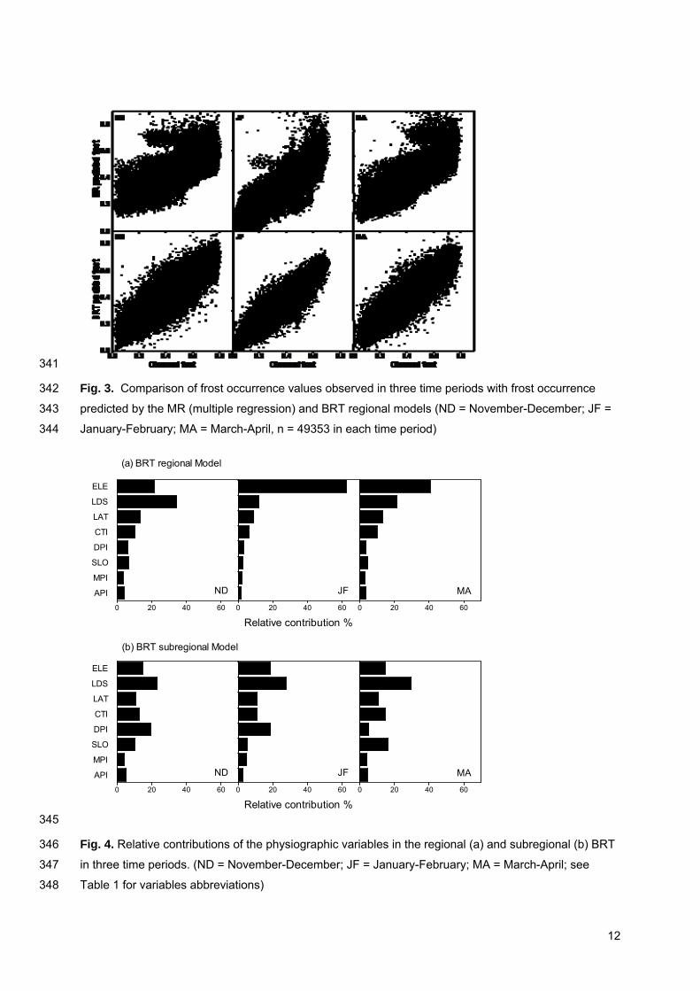
Regional BRT showed large effects of elevation, distance from the salt lakes, latitude and CTI on 328

frost occurrence, while slope and insolation variables had only marginal influence (Fig. 4a). Comparing 329

the three time periods, the relative contributions of the predictive variables showed some variations, 330

with the distance from the salt lakes dominating in the initial period (November-December), while 331

elevation became more important from January to April, and particularly in the mid-summer period. In 332

contrast, latitude, CTI and insolation variables kept a fairly constant effect with similar contributions at 333

the beginning and at the end of the season. Calibrating BRT models over a limited spatial domain 334

reveals slightly different patterns in the contributions of the predictors (Fig. 4b): distance from the salt 335

lakes gained importance on elevation in the three time periods, and daily potential insolation showed 336

noticeable contribution until mid-summer (though the influence of its morning and afternoon 337

components remained marginal). The weights of CTI and latitude were intermediate whatever the time 338

period, while the contribution of slope became important by the end of the season. 339

340

12

341

Fig. 3. Comparison of frost occurrence values observed in three time periods with frost occurrence 342

predicted by the MR (multiple regression) and BRT regional models (ND = November-December; JF = 343

January-February; MA = March-April, n = 49353 in each time period) 344

 

0 20 40 60

API

MPI

SLO

DPI

CTI

LAT

LDS

ELE

ND

0 20 40 60

JF

Relative contribution %

0 20 40 60

MA

0 20 40 60

API

MPI

SLO

DPI

CTI

LAT

LDS

ELE

ND

0 20 40 60

JF

Relative contribution %

0 20 40 60

MA

(a) BRT regional Model

(b) BRT subregional Model

345

Fig. 4. Relative contributions of the physiographic variables in the regional (a) and subregional (b) BRT 346

in three time periods. (ND = November-December; JF = January-February; MA = March-April; see 347

Table 1 for variables abbreviations) 348

13

3.2.3. Partial dependence in regional and subregional BRT 349

The plots of partial dependence for frost occurrence in the regional BRT (Fig. 5) indicate that frost 350

events in the study area occur mostly at high and medium latitude, increase continuously up to 4500 m 351

elevation, and are more frequent far away from the salt lakes. Concave positions (high CTI values) are 352

more prone to frost, and low daily potential insolation in those shaded areas also increases frost 353

occurrence at night, though separating the morning and afternoon components of the daily insolation 354

gives opposite results (data not shown). The dependence of frost occurrence on slope steepness 355

remained fairly constant. These partial responses of frost occurrence to the most active physiographic 356

variables show only limited seasonal changes. 357

 

3500 4000 4500 5000 5500

-0.2

0.0

0.2

Elevation (m)

Par

tial d

epen

denc

e

3.0 3.5 4.0 4.5 5.0 5.5LDS

-22 -21 -20 -19

-0.2

0.0

0.2

Latitude (decimal degree)

Par

tial d

epen

denc

e

6 8 10 12 14

CTI

5400 6400 7400 8400

-0.1

0.0

0.1

DPI (W m-2)

Par

tial d

epen

denc

e

0 10 20 30

Slope (degree)

358

Fig. 5. Partial dependence plots of the six most influential physiographic variables in the regional BRT 359

in three time periods (continuous line: November-December, dashed line: January-February, dotted 360

line: March-April; ticks at the inside top of the plots show deciles of site distribution across the variable; 361

see Table 1 for variables abbreviations). 362

More details emerge from the partial dependence plots of interactions in subregional BRT (Fig. 6 363

illustrating the January-February period, with similar results in the other two periods). For instance, up 364

to a distance of 10 km from the salt lakes (LDS ≈ 4.0) the effect of elevation on frost occurrence is low 365

and nearly constant below 3900 m, and then rises gradually above that level. But farther than 10 km 366

14

away from the salt lake borders, frost occurrence first decreases as elevation rises up to 3900 m and 367

then increases sharply above. This suggests that thermal inversions at night are more frequent at 368

distance from the salt lakes. Considering the interaction of elevation with CTI, while frost occurrence at 369

low elevation increases gradually up to CTI values of 9 and more sharply thereafter (concave 370

situations), at high elevation the effect of CTI is already important at values below 8 and then rose only 371

marginally. The effect of landscape concavity thus appears prominent at low elevation, where cold air 372

can accumulate in local depressions, while it becomes negligeable at high elevation where crests and 373

peaks dominate. 374

LDS

3.0

3.5

4.0

4.5

ELE3700

38003900

40004100

pred

icted fro

sk risk

0.0

0.1

0.2

0.3

0.4

375

 

CTI

7

8

9

10

ELE3700

38003900

40004100

pre

dicte

d fro

sk risk

0.00

0.05

0.10

0.15

0.20

0.25

376

Fig. 6. Joint partial dependence plots of some interactions between topographic variables in the 377

subregional BRT of the January-February period (see Table 1 for variables abbreviations). 378

379

15

Table 2. Validation statistics of frost occurrence multiple regression (MR) and boosted regression trees 380

(BRT) models calibrated over the entire study area (regional models) or the Intersalar area (subregional 381

models). B: bias; RMSE: root mean square error of prediction; R2: determination coefficient of the 382

regression line between observed and predicted values. ND = November-December; JF = January-383

February; MA = March-April. 384

385

Calibration procedure Period B RMSE R2

Regional MR (n = 49353) ND 2.7 10-5 0.129 0.45

JF 2.1 10-4 0.093 0.72

MA 8.5 10-4 0.110 0.59

Regional BRT (n = 49353) ND 1.7 10-5 0.082 0.78

JF 0.5 10-5 0.057 0.90

MA 0.6 10-5 0.071 0.83

Subregional BRT (n = 275) ND 2.9 10-5 0.062 0.80

JF 1.4 10-3 0.031 0.82

MA 2.9 10-3 0.049 0.82

386

3.3. Fine resolution frost occurrence maps 387

Regional BRT were used in prediction to downscale frost occurrence maps from the 1-km to the 388

100-m scale. The statistical validation conducted on reaggregated 1-km pixel clusters shows good fit 389

between predicted and observed (remotely sensed) frost occurrence values (Table 3), with RMSE of 390

predicted values of the same order than in the BRT regional model directly applied at the 1-km 391

resolution (Table 2). The 100-m scale maps display topoclimatic variations resulting in a detailed 392

zonation of frost occurrence. As an example, Fig. 7c-d shows that flat areas surrounding Mount Tunupa 393

are more prone to frost occurrence than the slopes of the volcano up to an elevation of approximately 394

4000 m, while sites located at higher altitudes are naturally colder. All over this area, east-facing slopes 395

appear less exposed to frost than west-facing slopes. In some particular places at the west, cold air 396

stagnation is also identifiable in the lower parts of local depressions. Such details were not visible on 397

the 1-km resolution map (Fig. 7b). 398

Table 3. Statistical comparison of 100-m frost occurrence predictions reaggregated at 1-km with 399

observed 1-km frost occurrence values (n = 49353). B: bias; RMSE: root mean square error of 400

prediction; R2: determination coefficient of the regression line between observed and predicted values. 401

ND = November-December; JF = January-February; MA = March-April. 402

Period B RMSE R2

ND 0.0252 0.0925 0.74

JF 0.0008 0.0644 0.87

MA 0.0543 0.0945 0.80

403

16

404

Fig. 7. Elevation map of the Mount Tunupa area (a), and frost occurrence in the March-April period 405

mapped at 1-km resolution from MODIS observations (b), at 100-m resolution (c) and in 3-D view using 406

regional BRT (d). Frost occurrence is scaled between 0 and 1 as the probability of daily occurrence of 407

negative Ts values in the March-April period. 408

409

3.4. Lapse rate estimation 410

Table 4 shows significant seasonal variations in the average lapse rate in land surface night 411

temperature calculated over the study area, with statistically stronger values in the mid-summer period 412

(-0.64 °C/100 m) in comparison with the beginning or the end of the season (ca. -0.60 °C/100 m). The 413

17

linear relationship between elevation and temperature was also greater in mid-summer compared to the 414

other two periods. The spatio-temporal variability in lapse rates was high since the coefficients of 415

variation were between 24 and 35% in the successive time periods, with lower variation in the mid-416

summer. 417

Table 4. Descriptive statistics of lapse rates of land surface temperature at night in three successive 418

time periods. 419

Period Mean (°C/100 m)

Coefficient of variation (%)

Coefficient of determination

Sample size

November - December -0.609 35.5 0.50 366

January - February -0.642 24.3 0.68 355

March - April -0.598 29.8 0.56 361

420

4. Discussion 421

The present study provides the first application of MODIS products to characterize frost occurrence 422

over a 45000 km² area in the Andean highlands. Frost occurrence over the summer period was either 423

calculated directly from land surface temperature remotely sensed at a 1-km scale, or estimated and 424

downscaled at 100-m by means of physiographic modeling. To our knowledge this is also the first 425

application of BRT in physiographic modeling. Both techniques are complementary in characterizing 426

frost occurrence: remote sensing brings spatialized and repetitive information on land surface 427

temperature and physiographic features, while BRT allow to explore the relative contribution of 428

physiographic factors at various scales and, hence, to downscale satellite information to a level 429

appropriate to farming and land management applications. 430

4.1. Application of remote sensing data for frost occurrence characterization 431

As pointed by François et al. (1999) at least three factors may potentially affect the relation between 432

Ts and Tn records: a difference in time (ca. 6 a.m. for minimum night air temperature versus 2 a.m. for 433

satellite radiative temperature), a difference in height (1.5 m above the soil surface for meteorological 434

data versus land surface temperature for satellite data), and a difference in spatial resolution (ca. 100 435

m2 footprint for local meteorological data versus 1 km2 for satellite data). In spite of this, these authors 436

observed only a stable shift of some degrees between Tn records in the Bolivian altiplano and Ts 437

registered at 2 a.m. with a 1-km spatial resolution by the NOAA/AVHRR satellite. A similar result was 438

found in the present study showing a linear and highly significant correlation of MODIS land surface 439

temperature at night with minimum air temperature recorded in meteorological stations (R2 = 0.81). 440

However, this validation may be biased since, as in most mountain areas in the world, the available 441

meteorological records are likely not representative of the most elevated and isolated parts of the study 442

area. Regarding the MODIS satellite, recent studies have improved and validated its calibration 443

algorithm for land surface temperature in various situations encompassing Bolivian highlands, semiarid 444

and arid regions, or nighttime/daytime overpasses (Wan, 2008; Wang et al., 2008). This ensures the 445

reliability of MODIS temperature data in the study area in spite of its specific location in cold and arid 446

tropical highlands. After verifying for the normality of the distribution of Ts data, the probability of frost 447

18

occurence can be easily calculated from the available satellite data series (eq. (1)). It should be noted 448

that the available series of 6-year daily records was long enough to statistically characterize frost 449

occurrence at the standard meteorological threshold of 0 °C, but not at lower temperature levels due 450

the scarcity of observations of severe frost events over the considered period. Frosts at -4 or -7 °C 451

would, however, be more relevant for agroclimatic purposes since they correspond to the frost tolerance 452

levels of major Andean crops such as potato and quinoa (Bois et al., 2006; Garcia et al., 2007; Geerts 453

et al., 2006; Jacobsen et al., 2005). This limitation should progressively disappear as the MODIS 454

archives grow and allow for the statistical evaluation of less frequent (and more severe) frost events. 455

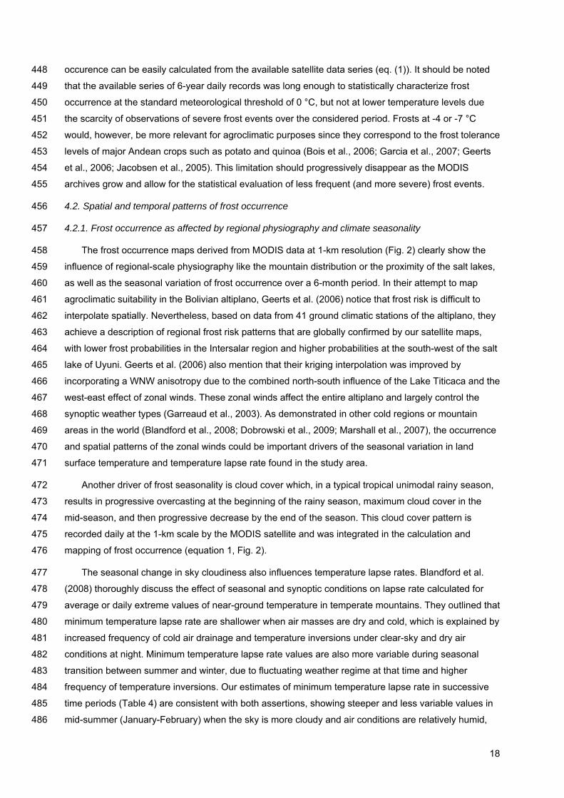
4.2. Spatial and temporal patterns of frost occurrence 456

4.2.1. Frost occurrence as affected by regional physiography and climate seasonality 457

The frost occurrence maps derived from MODIS data at 1-km resolution (Fig. 2) clearly show the 458

influence of regional-scale physiography like the mountain distribution or the proximity of the salt lakes, 459

as well as the seasonal variation of frost occurrence over a 6-month period. In their attempt to map 460

agroclimatic suitability in the Bolivian altiplano, Geerts et al. (2006) notice that frost risk is difficult to 461

interpolate spatially. Nevertheless, based on data from 41 ground climatic stations of the altiplano, they 462

achieve a description of regional frost risk patterns that are globally confirmed by our satellite maps, 463

with lower frost probabilities in the Intersalar region and higher probabilities at the south-west of the salt 464

lake of Uyuni. Geerts et al. (2006) also mention that their kriging interpolation was improved by 465

incorporating a WNW anisotropy due to the combined north-south influence of the Lake Titicaca and the 466

west-east effect of zonal winds. These zonal winds affect the entire altiplano and largely control the 467

synoptic weather types (Garreaud et al., 2003). As demonstrated in other cold regions or mountain 468

areas in the world (Blandford et al., 2008; Dobrowski et al., 2009; Marshall et al., 2007), the occurrence 469

and spatial patterns of the zonal winds could be important drivers of the seasonal variation in land 470

surface temperature and temperature lapse rate found in the study area. 471

Another driver of frost seasonality is cloud cover which, in a typical tropical unimodal rainy season, 472

results in progressive overcasting at the beginning of the rainy season, maximum cloud cover in the 473

mid-season, and then progressive decrease by the end of the season. This cloud cover pattern is 474

recorded daily at the 1-km scale by the MODIS satellite and was integrated in the calculation and 475

mapping of frost occurrence (equation 1, Fig. 2). 476

The seasonal change in sky cloudiness also influences temperature lapse rates. Blandford et al. 477

(2008) thoroughly discuss the effect of seasonal and synoptic conditions on lapse rate calculated for 478

average or daily extreme values of near-ground temperature in temperate mountains. They outlined that 479

minimum temperature lapse rate are shallower when air masses are dry and cold, which is explained by 480

increased frequency of cold air drainage and temperature inversions under clear-sky and dry air 481

conditions at night. Minimum temperature lapse rate values are also more variable during seasonal 482

transition between summer and winter, due to fluctuating weather regime at that time and higher 483

frequency of temperature inversions. Our estimates of minimum temperature lapse rate in successive 484

time periods (Table 4) are consistent with both assertions, showing steeper and less variable values in 485

mid-summer (January-February) when the sky is more cloudy and air conditions are relatively humid, 486

19

temperate, and stable. These estimates approximating –0.6 °C/100 m appear fairly high compared to 487

minimum temperature lapse rate values, typically ranging from –0.15 to –0.35 °C/100 m, in mountains 488

of mid-latitude regions (Blandford et al., 2008; Dobrowski et al., 2009; Harlow et al., 2004). In 489

subtropical mountains however, De Scally (1997 ) states that, due to their high thermal regime, the 490

temperature lapse rate is generally higher than in mid-latitude mountains. The high lapse rate values 491

thus quoted for the Himalaya (De Scally, 1997 ) or the Andes (Frère et al., 1978; Snow, 1975 cited by 492

Pielke & Mehring, 1977; Trombotto et al., 1997) refer unfortunately to mean daily or mean annual 493

temperatures which cannot be compared directly to our estimates of minimum temperature lapse rates 494

in specific time periods. 495

Astronomic forcing is another cause of seasonality in the topography-frost relationship, explaining 496

why topographic controls, usually treated as stationary, show actually pronounced seasonal variations, 497

as pointed by Deng et al. (2007) in the case of topography-vegetation relationships. In our study, 498

seasonal changes in the effects of slope steepness and aspect on frost occurrence are illustrated by 499

varying SLO and DPI contributions (Fig. 4b). They are explained by astronomical forcing resulting in 500

insolation values in the early and mid-summer higher by 25% in average than in the late-summer period 501

(see Table 1), thus giving higher influence of DPI over SLO in the former two periods. 502

Fig. 2 shows that the shores of the salt lakes are less prone to frost, while highlands at the west 503

and south of the region are continuously exposed, even in mid-summer (January-February) when frost 504

occurrence is generally low. This latter situation is obviously due to extreme elevation, while the 505

"milding" effect of the salt lakes could be due to the specific thermal properties of these vast salted 506

extenses. François et al. (1999) observed warmer night temperatures over the Coipasa and Uyuni salt 507

lakes and suggest that water covering these lakes part of the summer, as well as the higher thermal 508

conductivity and thermal capacity of the salted substratum, could explain that their borders remain 509

warmer than the surrounding areas. 510

4.2.2. From regional to subregional physiographic influences on frost occurrence 511

Multiple regression methods were used in previous studies to evaluate the relative contribution of 512

topographic factors to near-ground temperature and frost occurrence. These studies were generally 513

conducted in mid- or high-latitude mountains (Bennie et al., 2009; Chuanyan et al., 2005; Dobrowski et 514

al., 2009), and often in densely forested areas at mid-altitude (Blennow, 1998; Lindkvist et al., 2000; 515

Pypker et al., 2007b). Our study explored an extended agricultural region at its extreme elevation limit in 516

cold and arid tropical highlands. In this context, BRT models clearly outperformed multiple regression 517

models, probably due to their capacity to include nonlinear effects and interactions between predictors 518

(Martin et al., 2009). At the regional scale, BRT analyses show that elevation, distance to the salt lakes 519

and latitude were the physiographic features most contributing to frost occurrence variations, while 520

features directly or indirectly related to slope or topographic convergence (SLO, CTI, DPI, API, and 521

MPI) were less important. These regional BRT models based on physiographic features alone explain 522

between 78% and 90% of the variation in frost occurrence observed in different time periods (Table 2). 523

In their study of the influence of physiography on the distribution of climate variables across the United 524

States, Daly et al. (2008) outline that the effects of elevation and proximity to large water bodies exceed 525

20

those of other topographic factors at large scales, whereas the effects of slope and landcover features 526

become prominent at relatively smaller scales. In complex terrains, local variations in slope aspect and 527

steepness create a mosaic of hillslopes experiencing contrasting climatic regimes (Daly et al., 2008), 528

while topographic depressions are another landscape feature commonly associated with cold air 529

drainage and frost occurrence (Lundquist et al., 2008; Pypker et al., 2007b). These local landform 530

features emerge as forcing factors of frost occurence at the local scale, where the range of variation in 531

elevation and latitude became limited while that in local landscape features remained large. When 532

applied to the reduced spatial domain of the Intersalar, our BRT analyses indeed showed that elevation 533

lost some importance at the benefit of daily potential insolation (DPI), slope steepness (SLO), or 534

topographic convergence (CTI) (Fig. 4b). As a major characteristic of the physiography of south-535

western Bolivia, the vast salt lakes of Coipasa and Uyuni remained influential at that local scale, as 536

shown by the high contribution of the distance to the salt lakes (LDS) in these BRT subregional models. 537

The good fit of frost occurrence values predicted by BRT models applied either at the 100-m or the 1-538

km resolution (Tables 2 and 3) validates the use of BRT regional models for local frost occurrence 539

estimations since these models were able to seize both the influences of large-scale factors like latitude 540

and elevation, and of local factors like slope steepness, insolation, and landscape position. The 541

resulting local mosaic of cold depressions and warmer slopes at particular elevations and exposures is 542

illustrated by the map in Fig. 7c. We hypothesized that small-scale variations in soil warming due to 543

differential insolation in the day before (or the morning after) a given night could influence soil cooling 544

and thus radiative frost at night in particular places. In fact, the contribution of DPI appeared significant 545

in the BRT subregional model, at least from November to February when potential insolation is at its 546

seasonal maximum (Table 1), thus leading to highest contrasts in soil energy balance between sunlit 547

and shaded locations. However, the small contributions of the afternoon or morning components of 548

insolation (API and MPI) (Fig. 4b) seem to belie the idea that potential insolation is directly involved in 549

frost vulnerability at particular places. Actually, Blennow (1998) states that the larger amount of heat 550

stored into the ground in sunlit places cannot compensate for soil cooling at night since this cooling 551

occurs within a few hours after sunset. Nocturnal soil cooling should be still faster under clear-sky 552

conditions at high altitude. This is, however, in contradiction with the common perception of lower frost 553

occurrence in sunlit slopes, particularly in stony terrains and shallow soils supposed to benefit from the 554

thermal stability provided by the rocks. Microclimate stability associated to rock outcrops has been 555

documented by Rada et al. (2009) in the paramo ecosystem of Venezuelian Andes at lower elevation 556

(3800 m) and under wetter conditions (969 mm of annual precipitation). It is likely that the much drier 557

conditions of the puna ecosystem in southern Bolivia reduce the thermal inertia of the soils, thus leading 558

to a very fast soil cooling at night. Apart from astronomical forcing discussed previously, the varying 559

importance of CTI, DPI and SLO in the BRT models, as well as the interactions between them (Fig. 6) 560

reflect complex spatio-temporal relations between insolation and landform factors producing 561

multiplicative or mitigating effects on near-ground temperature. At the microscale level, unobserved soil 562

and vegetation properties might also interfere with landform features. Soil moisture and vegetation 563

cover, for example, are known to influence the radiative balance at the soil surface, and might 564

contribute to buffer the near-ground temperature from cold extremes in particular places (Fridley, 2009; 565

Geiger, 1971). 566

21

4.3. Ecological implications 567

The relationships between ecological patterns and processes change across spatial and temporal 568

scales, with singular complexity in mountain areas (e.g., Deng et al., 2007; Saunders et al., 1998). 569

Regarding air or soil surface temperature in mountains, nested factors are interacting, from regional 570

synoptic weather forcing to local topoclimatic situations and microscale variations in vegetation cover 571

and soil moisture. All these factors in turn may dominate the distribution of temperatures, depending not 572

only on the dynamics of the situation (turbulent or stable, nighttime or daytime conditions…) but also on 573

the spatial and temporal scale of interest (from macroscale to microscale, from seasonal to 574

instantaneous). In this way, macroscale conditions of clear sky and calm nights are required for 575

radiative frost to occur, but the frequency and severity of these frost events are further increased by low 576

site position (or conversely, extremely high location) and, at still smaller scales, by vegetation 577

sparseness and soil surface dryness or roughness (De Chantal et al., 2007; Fridley 2009; Langvall & 578

Ottonson Löfvenius, 2002; Oke, 1970). In the Andean highlands, instantaneous near-ground minimum 579

temperature may be 4°C lower in a sparsely vegetated area compared to a neighboring forest 580

understory (Rada et al., 2009). Similar fine scale variations in minimum air temperature occur within 581

cultivated canopies despite the low plant cover of most Andean crop species (see Winkel et al., 2009, 582

for the quinoa crop). These local variations in minimum near-ground temperatures may be sufficient for 583

some part of the vegetation to escape lethal freezing. Potential frost impacts on vegetation operating at 584

regional and subregional scales may thus be over-shadowed by microscale variability in minimum 585

temperature. Yet, contrary to what occurs in dense forests where plant interactions within canopies are 586

significant (Bader et al., 2008; Turnipseed et al., 2003), the sparse and low vegetation typical of the 587

Andean highlands is likely to exert an influence limited to small spatial scales, with topography and 588

coarse scale factors controlling most of the variation in minimum air temperature. In fact, Blennow 589

(1998) outlines that topographic influences on minimum air temperature increase in parallel with 590

decreasing vegetation cover. 591

4.4. Practical implications 592

The latter consideration implies that agroclimatic applications, such as crop zonation or suitability 593

assessments, require a multi-scale approach, ideally complementing frost risk characterization at the 594

topoclimatic scale by an evaluation of the local effects of crop practices on canopy structure and soil 595

surface moisture and roughness. Though limited to topography-frost relationships, our attempt of 596

downscaling frost occurrence at a 100-m scale usefully expands previous works on regional 597

agroclimatic zoning in the Bolivian altiplano (François et al., 1999; Geerts et al., 2006). To our 598

knowledge, this is the first time that such a detailed zonation of topoclimate is reported for this region, 599

providing fine-scale information helpful for land management and rural planning (Theobald et al., 2005). 600

Considering the scarcely available meteorological records in the study area, these 100-m scale maps 601

bring new information about the spatio-temporal variation of frost occurrence, allowing now to localize 602

exactly the seasonal pattern of frost typical of the Andean summer period (Frère et al., 1978; Troll, 603

1968). For instance, the virtual zero value of frost frequency in January and February derived from 604

meteorological records at Salinas (Fig. 1), covers in reality a wide range of situations with still significant 605

frost occurrence in mid-summer, as on the nearby border of the salar of Coipasa or the western and 606

22

southern part of the study area (Fig. 2). In fact, the recent expansion of quinoa crop in the region was 607

firstly and mostly located in flat areas near the Coipasa and Uyuni salt lakes (Vassas et al., 2008), 608

which exemplifies the complex trade-offs between agroclimatic risks and economic expectancies 609

operating in farmers' decision making (Luers 2005; Sadras et al., 2003). 610

4.5. Perspectives 611

Through remote sensing of land surface temperature and modeling of topographic features 612

implemented within a boosted regression procedure, we were able to explicitly downscale frost 613

occurrence at the landscape scale. The method developed here may be adapted to climatic or 614

ecological processes other than frost. Rainfall distribution could be a candidate since its spatio-temporal 615

patterns clearly depends on landscape characteristics over complex terrains. Current litterature outlines 616

the importance of landform as a factor of rainfall variability in the Andes (Giovannettone & Barros, 617

2009), though most studies were conducted at the coarse spatial resolution appropriate to continental 618

scale climatology (Garreaud & Aceituno, 2001; Misra et al., 2003; Vuille et al., 2003). Canopy energy 619

budget, soil water balance, or ecosystem productivity are other ecological processes tractable for 620

topographic modeling (Bradford et al., 2005; Rana et al., 2007; Urban et al., 2000). Such applications 621

depend firstly on the availability of remotely sensed proxies for the considered process. For example, 622

the remotely sensed daily amplitude in surface temperature and vegetation indices can be used to 623

derive daily evapotranspiration (Wang et al., 2006). Similarly, satellite estimates of absorbed 624

photosynthetically active radiation may serve to evaluate net primary productivity (Bradford et al., 2005; 625

Turner et al., 2009). An additional requisite for the calibration of these applications consists in local 626

ground measurements for the variable of interest. This is a major issue in the case of the tropical 627

highlands where, similarly to what occurs for meteorological data, reliable datasets on matter and 628

energy fluxes at ground level are and will remain scarce (Vergara et al., 2007). The methods and 629

results presented here can contribute to a better understanding of the potential risks associated with 630

climate and land use changes in complex terrains, so that decision-makers can develop efficient 631

strategies to improve the ecological sustainability of natural and agricultural ecosystems in vulnerable 632

mountain areas. 633

Acknowledgements 634

The authors are most grateful to Danny Lo Seen (Cirad, France) for discussions on BRT methods. 635

They also aknowledge the comments made by the anonymous reviewers of the paper. This work was 636

carried out with the financial support of the ANR (Agence Nationale de la Recherche - The French 637

National Research Agency) under the Programme "Agriculture et Développement Durable", project 638

"ANR-06-PADD-011-EQUECO". 639

References 640

Bader, M.Y., Rietkerk, M., & Bregt, A.K. (2008). A simple spatial model exploring positive feedbacks at 641

tropical alpine treelines. Arctic, Antarctic, and Alpine Research, 40, 269-278. 642

Bader, M.Y., & Ruijten, J.J.A. (2008). A topography-based model of forest cover at the alpine tree line in 643

the tropical Andes. Journal of Biogeography, 35, 711-723. 644

23

Benavides, R., Montes, F., Rubio, A., & Osoro, K. (2007). Geostatistical modelling of air temperature in 645

a mountainous region of Northern Spain. Agricultural and Forest Meteorology, 146, 173-188. 646

Bennie, J.J., Wiltshire, A.J., Joyce, A.N., Clark, D., Lloyd, A.R., Adamson, J., Parr, T., Baxter, R., & 647

Huntley, B. (2009). Characterising inter-annual variation in the spatial pattern of thermal microclimate in 648

a UK upland using a combined empirical-physical model. Agricultural and Forest Meteorology, 150, 12-649

19. 650

Blandford, T.R., Humes, K.S., Harshburger, B.J., Moore, B.C., Walden, V.P., & Ye, H. (2008). Seasonal 651

and synoptic variations in near-surface air temperature lapse rates in a mountainous basin. Journal of 652

Applied Meteorology and Climatology, 47, 249-261. 653

Blennow, K. (1998). Modelling minimum air temperature in partially and clear felled forests. Agricultural 654

and Forest Meteorology, 91, 223-235. 655

Blennow, K., & Lindkvist, L. (2000). Models of low temperature and high irradiance and their application 656

to explaining the risk of seedling mortality. Forest Ecology and Management, 135, 289-301. 657

Bois, J.F., Winkel, T., Lhomme, J.P., Raffaillac, J.P., & Rocheteau, A. (2006). Response of some 658

Andean cultivars of quinoa (Chenopodium quinoa Willd.) to temperature: effects on germination, 659

phenology, growth and freezing. European Journal of Agronomy, 25, 299-308. 660

Bradford, J.B., Hicke, J.A., & Lauenroth, W.K. (2005). The relative importance of light-use efficiency 661

modifications from environmental conditions and cultivation for estimation of large-scale net primary 662

productivity. Remote Sensing of Environment, 96, 246-255. 663

Chen, J., Saunders, S.C., Crow, T.R., Naiman, R.J., Brosofske, K.D., Mroz, G.D., Brookshire, B.L., & 664

Franklin, J.F. (1999). Microclimate in forest ecosystem and landscape ecology. Bioscience, 49, 288-665

297. 666

Chuanyan, Z., Zhongren, N., & Guodong, C. (2005). Methods for modelling of temporal and spatial 667

distribution of air temperature at landscape scale in the southern Qilian mountains, China. Ecological 668

Modelling, 189, 209-220. 669

Daly, C., Halbleib, M., Smith, J.I., Gibson, W.P., Doggett, M.K., Taylor, G.H., Curtis, J., & Pasteris, P.P. 670

(2008). Physiographically sensitive mapping of climatological temperature and precipitation across the 671

conterminous United States. International Journal of Climatology, 28, 2031-2064. 672

De Chantal, M., Hanssen, K.H., Granhus, A., Bergsten, U., Lofvenius, M.O., & Grip, H. (2007). Frost-673

heaving damage to one-year-old Picea abies seedlings increases with soil horizon depth and canopy 674

gap size. Canadian Journal of Forest Research, 37, 1236-1243. 675

De Scally, F.A. (1997 ). Deriving lapse rates of slope air temperature for meltwater runoff modeling in 676

subtropical mountains: an exemple from the Punjab Himalaya. Moutain Research and Development, 677

17, 353-362. 678

Del Castillo, C., Mahy, G., & Winkel, T. (2008). Quinoa in Bollivia: an ancestral crop changed to a cash 679

crop with "organic fair-trade" labeling. Biotechnologie, Agronomie, Société et Environnement (BASE), 680

12, 421-435. 681

24

Deng, Y., Chen, X., Chuvieco, E., Warner, T., & Wilson, J.P. (2007). Multi-scale linkages between 682

topographic attributes and vegetation indices in a mountainous landscape. Remote Sensing of 683

Environment, 111, 122-134. 684

Dobrowski, S.Z., Abatzoglou, J.T., Greenberg, J.A., & Schladow, S.G. (2009). How much influence 685

does landscape-scale physiography have on air temperature in a mountain environment? Agricultural 686

and Forest Meteorology, 149, 1751-1758. 687

Elith, J., Leathwick, J.R., & Hastie, T. (2008). A working guide to boosted regression trees. Journal of 688

Animal Ecology, 77, 802-813. 689

Farr, T.G., Rosen, P.A., Caro, E., Crippen, R., Duren, R., Hensley, S., Kobrick, M., Paller, M., 690

Rodriguez, E., Roth, L., Seal, D., Shaffer, S., Shimada, J., Umland, J., Werner, M., Oskin, M., Burbank, 691

D., & Alsdorf, D. (2007). The shuttle radar topography mission. Reviews of Geophysics, 45, RG2004, 692

doi: 2010.1029/2005RG000183. 693

François, C., Bosseno, R., Vacher, J.J., & Seguin, B. (1999). Frost risk mapping derived from satellite 694

and surface data over the Bolivian Altiplano. Agricultural and Forest Meteorology, 95, 113-137. 695

Frère, M., Rijks, J.Q., & Rea, J. (1978). Estudio agroclimatológico de la zona andina. Nota Técnica n° 696

161. (373 p.). Ginebra, Suiza: Proyecto interinstitucional FAO/UNESCO/OMM. Organización 697

Meteorológica Mundial. 698

Fridley, J.D. (2009). Downscaling climate over complex terrain: high finescale (<1000 m) spatial 699

variation of near-ground temperatures in a montane forested landscape (Great Smoky Mountains). 700

Journal of Applied Meteorology and Climatology, 48, 1033-1049. 701

Friedman, J.H., & Meulman, J.J. (2003). Multiple additive regression trees with application in 702

epidemiology. Statistics in Medicine, 22, 1365-1381. 703

Fu, P., & Rich, P.M. (2002). A geometric solar radiation model with applications in agriculture and 704

forestry. Computers and Electronics in Agriculture, 37, 25-35. 705

Garcia, M., Raes, D., Allen, R., & Herbas, C. (2004). Dynamics of reference evapotranspiration in the 706

Bolivian highlands (Altiplano). Agricultural and Forest Meteorology, 125, 67-82. 707

Garcia, M., Raes, D., Jacobsen, S.E., & Michel, T. (2007). Agroclimatic constraints for rainfed 708

agriculture in the Bolivian Altiplano. Journal of Arid Environments, 71, 109-121. 709

Garreaud, R., Vuille, M., & Clement, A.C. (2003). The climate of the Altiplano: observed current 710

conditions and mechanisms of past changes. Palaeogeography, Palaeoclimatology, Palaeoecology, 711

194 5-22. 712

Garreaud, R.D., & Aceituno, P. (2001). Interannual rainfall variability over the South American altiplano. 713

Journal of Climate, 14, 2779-2789. 714

Geerts, S., Raes, D., Garcia, M., Del Castillo, C., & Buytaert, W. (2006). Agro-climatic suitability 715

mapping for crop production in the Bolivian Altiplano: a case study for quinoa. Agricultural and Forest 716

Meteorology, 139, 399-412. 717

25

Geiger, R. (1971). The climate near the ground. Cambridge, MA, USA: Harvard University Press. 718

Gessler, P.E., Chadwick, O.A., Chamran, F., Althouse, L., & Holmes, K. (2000). Modeling soil-719

landscape and ecosystem properties using terrain attributes. Soil Science Society of America Journal, 720

64, 2046-2056. 721

Giovannettone, J.P., & Barros, A.P. (2009). Probing regional orographic controls of precipitation and 722

cloudiness in the central Andes using satellite data. Journal of Hydrometeorology, 10, 167-182. 723

Gonzalez, J.A., Gallardo, M.G., Boero, C., Liberman Cruz, M., & Prado, F.E. (2007). Altitudinal and 724

seasonal variation of protective and photosynthetic pigments in leaves of the world's highest elevation 725

trees Polylepis tarapacana (Rosaceae). Acta Oecologica, 32, 36-41. 726

Grötzbach, E., & Stadel, C. (1997). Mountain peoples and cultures. In B. Messerli & J.D. Ives (Eds.), 727

Mountains of the world: a global priority (pp. 17-38). New York, USA: The Partenon Publishing Group. 728

Harlow, R.C., Burke, E.J., Scott, R.L., Shuttleworth, W.J., Brown, C.M., & Petti, J.R. (2004). Derivation 729

of temperature lapse rates in semi-arid south-eastern Arizona. Hydrology and Earth System Sciences, 730

8, 1179-1185. 731

Hoch, G., & Körner, C. (2005). Growth, demography and carbon relations of Polylepis trees at the 732

world's highest treeline. Functional Ecology, 19, 941-951. 733

Jacobsen, S.E., Monteros, C., Christiansen, J.L., Bravo, L.A., Corcuera, L.J., & Mujica, A. (2005). Plant 734

responses of quinoa (Chenopodium quinoa Willd.) to frost at various phenological stages. European 735

Journal of Agronomy, 22, 131-139. 736

Langvall, O., & Ottonson Löfvenius, M. (2002). Effect of shelterwood density on nocturnal near-ground 737

temperature, frost injury risk and budburst date of Norway spruce. Forest Ecology and Management, 738

168, 149-161. 739

Lawrence, R., Bunn, A., Powell, S., & Zambon, M. (2004). Classification of remotely sensed imagery 740

using stochastic gradient boosting as a refinement of classification tree analysis. Remote Sensing of 741

Environment, 90, 331-336. 742

Lindkvist, L., Gustavsson, T., & Bogren, J. (2000). A frost assessment method for mountainous areas. 743

Agricultural and Forest Meteorology, 102, 51-67. 744

Lookingbill, T.R., & Urban, D.L. (2003). Spatial estimation of air temperature differences for landscape-745

scale studies in montane environments. Agricultural and Forest Meteorology, 114, 141-151. 746

Luers, A.L. (2005). The surface of vulnerability: an analytical framework for examining environmental 747

change. Global Environmental Change Part A, 15, 214-223. 748

Lundquist, J.D., Pepin, N., & Rochford, C. (2008). Automated algorithm for mapping regions of cold-air 749

pooling in complex terrain. Journal of Geophysical Research, 113, D22107 doi: 750

22110.21029/22008JD009879. 751

26

Marshall, S.J., Sharp, M.J., Burgess, D.O., & Anslow, F.S. (2007). Near-surface-temperature lapse 752

rates on the Prince of Wales Icefield, Ellesmere Island, Canada: implications for regional downscaling 753

of temperature. International Journal of Climatology, 27, 385-398. 754

Martin, M.P., Lo Seen, D., Boulonne, L., Jolivet, C., Nair, K.M., Bourgeon, G., & Arrouays, D. (2009). 755

Optimizing pedotransfer functions for estimating soil bulk density using boosted regression trees. Soil 756

Science Society of America Journal, 73, 485-493. 757

Misra, V., Dirmeyer, P.A., & Kirtman, B.P. (2003). Dynamic downscaling of seasonal simulations over 758

South America. Journal of Climate, 16, 103-117. 759

Nagy, L., Grabherr, G., Körner, C., & Thompson, D.B.A. (Eds.) (2003). Alpine biodiversity in Europe. 760

Berlin, Germany: Springer Verlag. 761

Navarro, G., & Ferreira, W. (2007). Mapa de vegetación de Bolivie a escala 1:250.000. Santa Cruz de 762

la Sierra, Bolivia: The Nature Conservancy (TNC) 763

Oke, T.R. (1970). The temperature profile near the ground on calm clear nights. Quarterly Journal of the 764

Royal Meteorological Society, 96, 14-23. 765

Parisien, M.-A., & Moritz, M.A. (2009). Environmental controls on the distribution of wildfire at multiple 766

spatial scales. Ecological Monographs, 79, 127-154. 767

Pielke, R.A., & Mehring, P. (1977). Use of mesoscale climatology in mountainous terrain to improve 768

spatial representation of mean monthly temperatures. Monthly Weather Review, 105, 108-112. 769

Pypker, T.G., Unsworth, M.H., Lamb, B., Allwine, E., Edburg, S., Sulzman, E., Mix, A.C., & Bond, B.J. 770

(2007a). Cold air drainage in a forested valley: investigating the feasibility of monitoring ecosystem 771

metabolism. Agricultural and Forest Meteorology, 145, 149-166. 772

Pypker, T.G., Unsworth, M.H., Mix, A.C., Rugh, W., Ocheltree, T., Alstad, K., & Bond, B.J. (2007b). 773

Using nocturnal cold air drainage flow to monitor ecosystem processes in complex terrain. Ecological 774

Applications, 17, 702-714. 775

R Development Core Team (2006). R: a language and environment for statistical computing. Vienna, 776

Austria: R Foundation for Statistical Computing. 777

Rada, F., García-Núñez, C., & Rangel, S. (2009). Low temperature resistance in saplings and ramets of 778

Polylepis sericea in the Venezuelan Andes. Acta Oecologica, 35, 610-613. 779

Rana, G., Ferrara, R.M., Martinelli, N., Personnic, P., & Cellier, P. (2007). Estimating energy fluxes from 780

sloping crops using standard agrometeorological measurements and topography. Agricultural and 781

Forest Meteorology, 146, 116-133. 782

Ronchail, J. (1989). Advections polaires en Bolivie : mise en évidence et caractérisation des effets 783

climatiques. Hydrologie Continentale, 4, 49-56. 784

Sadras, V., Roget, D., & Krause, M. (2003). Dynamic cropping strategies for risk management in dry-785

land farming systems. Agricultural Systems, 76, 929-948. 786

27

Santibañez, F., Morales, L., de la Fuente, J., Cellier, P., & Huete, A. (1997). Topoclimatic modeling for 787

minimum temperature prediction at a regional scale in the Central Valley of Chile. Agronomie, 17, 307-788

314. 789

Saunders, S.C., Chen, J.Q., Crow, T.R., & Brosofske, K.D. (1998). Hierarchical relationships between 790

landscape structure and temperature in a managed forest landscape. Landscape Ecology, 13, 381-395. 791

StatSoft France (2005). STATISTICA (logiciel d'analyse de données), version 7.1: www.statsoft.fr 792

Snow, J. W. (1975). The climates of northern South America. M.Sc. Thesis, University of Wisconsin, 793

Madison. 238 pp. 794

Theobald, D.M., Spies, T., Kline, J., Maxwell, B., Hobbs, N.T., & Dale, V.H. (2005). Ecological support 795

for rural land-use planning. Ecological Applications, 15, 1906-1914. 796

Troll, C. (1968). The Cordilleras of the tropical Americas: aspects of climatic, phytogeographical and 797

agrarian ecology. In C. Troll (Ed.), Proceedings of the UNESCO Mexico Symposium, August 1-3 1966. 798

Colloquium Geographicum, vol.9 (pp. 15-56). Bonn, Germany: Ferd. Dümmlers Verlag. 799

Trombotto, D., Buk, E., & Hernández, J. (1997). Monitoring of mountain permafrost in the Central 800

Andes, Cordon del Plata, Mendoza, Argentina. Permafrost and Periglacial Processes, 8, 123-129. 801

Turner, D.P., Ritts, W.D., Wharton, S., Thomas, C., Monson, R., Black, T.A., & Falk, M. (2009). 802

Assessing FPAR source and parameter optimization scheme in application of a diagnostic carbon flux 803

model. Remote Sensing of Environment, 113, 1529-1539. 804

Turnipseed, A.A., Anderson, D.E., Blanken, P.D., Baugh, W.M., & Monson, R.K. (2003). Airflows and 805

turbulent flux measurements in mountainous terrain: Part 1. Canopy and local effects. Agricultural and 806

Forest Meteorology, 119, 1-21. 807

Urban, D., Miller, C., Halpin, P., & Stephenson, N. (2000). Forest gradient response in Sierran 808

landscapes: the physical template. Landscape Ecology, 15, 603-620. 809

Vassas, A., Vieira Pak, M., & Duprat, J.R. (2008). El auge de la quinua: cambios y perspectivas desde 810

una visión social. Habitat, 75: 31-35. 811

Vergara, W., Kondo, H., Pérez Pérez, E., Méndez Pérez, J.M., Magaña Rueda, V., Martínez Arango, 812

M.C., Ruíz Murcia, J.F., Avalos Roldán, G.J., & Palacios, E. (2007). Visualizing Future Climate in Latin 813

America: results from the application of the Earth Simulator. In (p. 82 p.): The World Bank, Latin 814

America and the Caribbean Region 815

Vuille, M., Bradley, R.S., Werner, M., & Keimig, F. (2003). 20th century climate change in the tropical 816

Andes: observations and model results. Climatic Change, 59, 75-99. 817

Vuille, M., Francou, B., Wagnon, P., Juen, I., Kaser, G., Mark, B.G., & Bradley, R.S. (2008). Climate 818

Change and tropical Andean glaciers: past, present and future. Earth-Science Reviews, 89, 79-96. 819

Wan, Z. (2008). New refinements and validation of the MODIS Land-Surface Temperature/Emissivity 820

products. Remote Sensing of Environment, 112, 59-74. 821

28

Wang, K., Li, Z., & Cribb, M. (2006). Estimation of evaporative fraction from a combination of day and 822

night land surface temperatures and NDVI: a new method to determine the Priestley-Taylor parameter. 823

Remote Sensing of Environment, 102, 293-305. 824

Wang, W., Liang, S., & Meyers, T. (2008). Validating MODIS land surface temperature products using 825

long-term nighttime ground measurements. Remote Sensing of Environment, 112, 623-635. 826

Winkel, T., Lhomme, J.P., Nina Laura, J.P., Mamani Alcón, C., Del Castillo, C., & Rocheteau, A. (2009). 827

Assessing the protective effect of vertically heterogeneous canopies against radiative frost: the case of 828

quinoa on the Andean Altiplano. Agricultural and Forest Meteorology, 149, 1759-1768. 829