
LAPPEENRANTA-LAHTI UNIVERSITY OF TECHNOLOGY (LUT)
LUT School of Energy Systems
Degree Programme in Energy Technology
Aapo Vuorinen
UTILIZING FEEDBACK CALCULATIONS IN DEVELOPMENT OF BUBBLING
FLUIDIZED BED BOILER DESIGN
Examiners: Professor, D.Sc. (Tech.) Esa Vakkilainen
Research Director, D.Sc. (Tech.) Juha Kaikko
Instructors: M.Sc. (Tech.) Jukka Hautamaa, Andritz Oy
M.Sc. (Tech.) Timo Itävuo, Andritz Oy
M.Sc. (Tech.) Janne Tiihonen, Prasinos Oy

ABSTRACT
Lappeenranta-Lahti University of Technology (LUT)
LUT School of Energy Systems
Degree Programme in Energy Technology
Aapo Vuorinen
Utilizing feedback calculations in development of bubbling fluidized bed boiler design
Master’s thesis
2020
103 pages, 25 figures, and 16 tables
Examiners: Professor, D.Sc. (Tech.) Esa Vakkilainen
Research Director, D.Sc. (Tech.) Juha Kaikko
Keywords: bubbling fluidized bed boiler, BFB, feedback, thermal design, dimensioning
The main objective of this thesis was to study and specify process design parameters utilized
in bubbling fluidized bed boiler design and dimensioning in Andritz Oy. More accurate
parameters could allow dimensioning heat transfer surfaces more precisely, reduce material
costs, and help achieve and improve performance guarantees. Aim of the thesis was also to
implement feedback calculations to be a part of the process design software and follow-up
routine.
Parameters were studied with a feedback (FB) model made for Solvo heat balance simulator
software. FB model is based on pre-existing design templates, and can be used for both
design- and feedback calculations in the future. Averaged measurement data from five
boilers and altogether 16 cases was used to iterate the real values for parameters. Calculation
procedure is based on an iteration routine that adjusts the parameter values until the
difference between simulated process values and averaged measurement results are within
tolerance.
Calculated parameters were found to be different from previous recommended parameter
values. Studied furnace parameters were higher than recommended, and increased
significantly when steam load decreased. Comparing to recommended parameter values,
calculated superheater 2 parameters were slightly lower, but other superheater and
economizer parameters were noticeably higher. Air preheater parameters were close to
recommended values. Results were quite reliable and validated with e.g. a semi-empirical
furnace model, but further studies and adjustments were recommended to improve the model
accuracy and reliability.
Based on the calculated design parameter values, the recommended values have not always
been accurate. Changes to recommended values were suggested, but the adjustments should
be conservative until more cases have been calculated and the accuracy of FB model results
more carefully studied and analyzed.

TIIVISTELMÄ
Lappeenrannan-Lahden teknillinen yliopisto (LUT)
LUT School of Energy Systems
Energiatekniikan koulutusohjelma
Aapo Vuorinen
Takaisinlaskennan hyödyntäminen kuplapetikattilan mitoituksen kehittämisessä
Diplomityö
2020
103 sivua, 25 kuvaa ja 16 taulukkoa
Tarkastajat: Professori, TkT Esa Vakkilainen
Dosentti, TkT Juha Kaikko
Hakusanat: kuplapetikattila, BFB, takaisinlaskenta, lämpötekninen suunnittelu, mitoitus
Tämän diplomityön tärkeimpänä tavoitteena oli tutkia ja tarkentaa Andritz Oy:n
kuplapetikattilan suunnittelussa ja mitoituksessa käytettyjä suunnitteluparametreja.
Tarkemmat parametrit voisivat mahdollistaa lämmönsiirtopintojen tarkemman mitoituksen,
vähentää materiaalikustannuksia ja auttaa saavuttamaan ja parantamaan suorituskykytakuita.
Työn tavoitteena oli myös implementoida takaisinlaskenta osaksi prosessisuunnittelu-
ohjelmistoa ja seurantarutiineja.
Parametreja tutkittiin takaisinlaskentamallilla, joka kehitettiin Solvo lämpötasesimulaatio-
ohjelmistolle. Takaisinlaskentamalli perustuu olemassa olleisiin suunnittelumallipohjiin, ja
sitä voidaan jatkossa käyttää sekä suunnitteluun että takaisinlaskentaan. Keskiarvoistettua
mittausdataa viidestä kattilasta ja yhteensä 16 tapauksesta käytettiin parametrien todellisten
arvojen iteroimiseen. Laskentamenetelmä perustuu iteraatiorutiiniin, joka säätää
parametrien arvoja, kunnes ero simuloitujen prosessiarvojen ja keskiarvoistettujen
mittaustulosten välillä on sallituissa rajoissa.
Laskettujen parametrien havaittiin poikkeavan edellisistä parametrien suositusarvoista.
Tutkitut tulipesäparametrit olivat korkeampia kuin suositeltu, ja ne kasvoivat merkittävästi
kun höyrykuorma laski. Parametrien suositusarvoihin verrattuna lasketut tulistin 2:n
parametrit olivat hieman matalampia, mutta muiden tulistimien ja ekonomaiserin parametrit
olivat selvästi korkeampia. Ilman esilämmittimien parametrit olivat lähellä suositusarvoja.
Tulokset olivat melko luotettavia ja validoitiin esimerkiksi semi-empiirisellä
tulipesämallilla, mutta jatkotutkimuksia ja –säätöjä suositeltiin mallin tarkkuuden ja
luotettavuuden parantamiseksi.
Laskettujen suunnitteluparametrien arvojen perusteella suositusarvot eivät ole aina olleet
tarkkoja. Muutoksia suositusarvoihin ehdotettiin, mutta muutokset tulisivat olla maltillisia
kunnes lisää tapauksia on laskettu ja takaisinlaskentamallin tuloksien tarkkuutta on
tarkemmin tutkittu ja analysoitu.

ACKNOWLEDGEMENTS
This Master’s thesis was done for Andritz Oy in Varkaus during the first half of the notorious
year of 2020. The time of COVID-19, winter that felt like fall, and endless hours between
the walls of my apartment. But now, in June, the weather seems out of this world (or rather:
out of this country), constrictions are starting to get lifted, and my graduation finally seems
inevitable.
I would like to thank my instructors Timo Itävuo and Janne Tiihonen for insightful
comments and different perspectives, as well as great ideas that helped me make the
feedback model functional and usable in the first place. I’m especially grateful to Jukka
Hautamaa for his continuous support, guidance, and challenging tasks even long before my
thesis.
I would also like to thank the personnel of my university for a great education and foundation
for my working career in the energy field. Special thanks to Professor Esa Vakkilainen for
guidance and comments on my thesis, as well as all the interesting lectures during my years
in Lappeenranta.
Last but not least, thank you Armatuuri Ry, friends and family for all the support,
experiences, and diversions from studies during all these years.
Varkaus, 26.6.2020
Aapo Vuorinen

TABLE OF CONTENTS
LIST OF SYMBOLS AND ABBREVIATIONS 8
1 INTRODUCTION 11
1.1 Objectives ................................................................................................ 11
1.2 Thesis structure ........................................................................................ 12
2 STEAM GENERATION AND BFB BOILER FUNDAMENTALS 13
2.1 Steam power plants and steam generation ............................................... 13
2.2 BFB boiler working principle .................................................................. 14
2.3 Bed fluidization theory ............................................................................ 15
2.4 Auxiliary systems .................................................................................... 17
2.5 Typical operating values, construction and components ......................... 20
2.6 Instrumentation, measurements and uncertainty ..................................... 25
2.6.1 Measurement methods ................................................................. 25
2.6.2 Measurement uncertainty ............................................................ 28
2.7 Heat transfer in BFB boilers .................................................................... 30
3 STUDIED BOILERS AND MEASUREMENTS 33
3.1 Boiler 1 .................................................................................................... 33
3.2 Boiler 2 .................................................................................................... 35
3.3 Boiler 3 .................................................................................................... 36
3.4 Boiler 4 .................................................................................................... 37
3.5 Boiler 5 .................................................................................................... 38
3.6 Measurement data .................................................................................... 39
4 DESIGN PROCESS AND PARAMETERS 41
4.1 Design software ....................................................................................... 41
4.2 Boiler models ........................................................................................... 41
4.3 Design parameters ................................................................................... 43
4.4 Inaccuracies and needs for development ................................................. 44
5 FEEDBACK CALCULATION MODELS 47
5.1 Target values ............................................................................................ 47

5.2 Iteration parameters ................................................................................. 48
5.3 Feedback calculation approaches ............................................................ 51
5.3.1 Base model with added controllers ............................................. 51
5.3.2 Block-model approach ................................................................ 53
5.3.3 Base model with macro controllers and external furnace iteration55
5.4 Feedback model ....................................................................................... 56
5.4.1 Model construction ...................................................................... 57
5.4.2 Feedback initialization ................................................................ 59
5.4.3 Iteration process .......................................................................... 59
5.4.4 Component iteration routine ........................................................ 62
5.4.5 HSS iteration routine ................................................................... 64
5.4.6 Furnace iteration process ............................................................. 66
5.5 Feedback model limitations and simplifications ..................................... 68
6 RESULTS 70
6.1 Initial conditions and basis for calculations............................................. 70
6.2 Process values .......................................................................................... 72
6.2.1 Mass flows ................................................................................... 72
6.2.2 Temperatures ............................................................................... 74
6.3 Design parameters ................................................................................... 78
6.3.1 Relative burner height ................................................................. 78
6.3.2 Superheaters ................................................................................ 79
6.3.3 3rd pass ........................................................................................ 82
6.3.4 Fuel moisture ............................................................................... 84
6.4 Result validation ...................................................................................... 85
6.4.1 Solvo design template ................................................................. 85
6.4.2 Furnace exit flue gas temperature ............................................... 86
6.5 Result reliability....................................................................................... 88
6.5.1 Boiler 1 ........................................................................................ 89
6.5.2 Boiler 2 ........................................................................................ 91
6.5.3 Boiler 3 ........................................................................................ 92
6.5.4 Boiler 4 ........................................................................................ 93
6.5.5 Boiler 5 ........................................................................................ 94

7 DISCUSSION AND CONCLUSIONS 95
7.1 Design parameters ................................................................................... 95
7.2 Recommended values for parameters ...................................................... 97
7.3 Future development ................................................................................. 99
7.4 Further studies ....................................................................................... 100
8 SUMMARY 102
REFERENCES 104

LIST OF SYMBOLS AND ABBREVIATIONS
Roman alphabet
A area m2
C coefficient -
d diameter m
Eb total emissive power of a blackbody W/m2
g gravitational acceleration m/s2
h convection heat transfer coefficient W/(m2K)
H height m
k thermal conductivity W/(mK)
Kf correction factor -
l flow approach length m
p pressure Pa
q heat rate W
T temperature K, °C
U overall heat transfer coefficient W/(m2K)
v velocity m/s
wρ density of mass flow rate kg/(m2s)
x position m
Greek alphabet
α absorptivity -
α the coefficient of heat transfer W/(m2K)
Δ difference -
ε emissivity -
ε share of empty volume in bed -
µ dynamic viscosity Ns/m2
ρ density m3/kg
σ Stefan-Boltzmann constant (5.67 ∙ 10-8) W/(m2K4)
Subscripts
∞ fluid
cond conduction

conv convection
d drag
g gas
mf minimum fluidizing
p particle
rad radiation
s sensor
s surface
t terminal
th thermal
w wall
Abbreviations
BB boiler bank (convective evaporator)
BFB bubbling fluidized bed
CBD continuous blow-down
CFB circulating fluidized bed
CHP combined heat and power
DCS digital control system
DPT differential pressure transmitter
ECO economizer
ESP electrostatic precipitator
FB feedback
FEGT furnace exit flue gas temperature
H2SO4 sulfuric acid
HCl hydrochloric acid
HSS heat shift system
ID induced draft
IR infrared
LUVO Luftvorwärmer (flue gas air preheater)
NOx nitrogen oxides
PFC pulverized fuel combustion
RBH relative burner height

RDF refuse-derived fuel
SCAH steam coil air preheater
SCR selective catalytic reduction
SH superheater
SNCR selective non-catalytic reduction
SO2 sulfur oxide
SRF solid recovered fuel

11
1 INTRODUCTION
Bubbling fluidized bed (BFB) boilers are commonly used for energy production by burning
a wide variety of fuels, especially volatile, solid biomass. In the effort of fighting climate
change, reducing the use of fossil fuels, and increasing biomass usage, advanced combustion
methods such as BFB become more and more prominent and advantageous.
Most BFB boilers are designed individually based on the specific customer requirements
and fuel range, which makes accurate dimensioning and design essential. If heat exchangers
are designed to be larger than needed, material costs would increase and the boiler could
operate inefficiently. On the other hand, if heat exchangers are designed to be too small, e.g.
steam requirements might not be met. Inaccuracies in both directions could lead to issues
with materials and temperatures around the boiler. Therefore, being able to design the boiler
process and heat transfer surfaces accurately is beneficial both in financial and operational
standpoint.
Feedback calculations can be conducted to determine how accurate the dimensioning of the
boilers originally were. In BFB boiler design, some parameters are hard or impossible to
calculate or know beforehand; therefore, typical values based on previous experience are
chosen. In feedback calculations these parameters are calculated based on known values,
such as heat transfer area, and measured values, such as temperatures and pressures.
Feedback results allow choosing the parameters more accurately in the future. Feedback
calculations are done with feedback models that are developed based on pre-existing design
models of boilers, and by using the same software that is used for dimensioning and design
of boiler process.
1.1 Objectives
One of the main objectives of this thesis is to allow implementing feedback calculations as
a fundamental part of new boiler design process at Andritz Oy. Feedback calculation routines
should be added to design- and dimensioning tools to continuously improve design process
and transparency. Results from feedback will indicate the accuracy of the design process and
provide valuable reference values for the future designs.

12
Another objective is to improve boiler dimensioning accuracy, reduce the margin of error,
and ultimately enable tighter performance guarantees. This can be achieved by using
measurement data from online measurements, guarantee tests or other sources to calculate
real values for design parameters. Calculated parameters can be compared to current
parameter recommendations, and help adjust the recommendations accordingly. In addition
to heat transfer theory or previous correlations, using design parameters that are validated
with feedback calculations will improve the reliability and accuracy of designed process
values in the future.
Final objective of this thesis is to provide potential to achieve financial benefits from more
accurate boiler design. If design values can be designed more accurately, safety factors could
be lowered and margin of error would reduce, which could potentially lead to lower material
costs and decreased need for rework. Having better guarantees, more accurate designs, and
potentially lower material costs could also help competitiveness of Andritz boilers.
1.2 Thesis structure
Chapter 2 consists of steam generation and BFB boilers basics. Theory about fluidization,
measurements, and heat transfer are discussed briefly. Overview of each studied boiler and
descriptions of their respective measurement periods used for calculations are presented in
chapter 3. Design software, design models, and motivation for development are discussed in
chapter 4.
The feedback calculation model is described in chapter 5. Different utilization of
measurement results, iteration parameters, and multiple approaches to calculations are
covered. The final version of the model, its principles, and its limitations are described and
discussed. Chapter 6 includes results from calculations, as well as further consideration of
result validation and reliability. Both calculated parameters and process value comparison
between measured and calculated values are discussed. Finally, new recommendations for
design parameters and ideas for future development and studies are presented in chapter 7,
following with a summary in chapter 8.

13
2 STEAM GENERATION AND BFB BOILER FUNDAMENTALS
The working principle and fundamentals of BFB boilers are discussed in this chapter. In
addition, typical construction and components are described. Measurement methods,
uncertainties, and heat transfer phenomena in BFB boilers are discussed as well, because
measurements and heat transfer calculations are crucial in this thesis.
2.1 Steam power plants and steam generation
Steam power plants are used to produce steam for electricity or heat generation. Steam is
generated in a boiler, where the released heat from fuel is transferred to water and steam.
The steam is transported to turbines, where the steam’s pressure and temperature decreases,
while rotating the turbine by expanding. Rotational energy of the turbine is converted to
electricity with a generator. Low-pressure steam is led to a condenser, where it condenses
back to water. Water is pumped and preheated again before it is transported back to the
boiler. The steam power plant process is based on Rankine cycle. (Huhtinen et al. 2004, 8-
15)
In a combined heat and power (CHP) plant steam isn’t expanded to as low a pressure as in a
pure electric power plant, and more steam power is extracted as heat. Electricity generation
is therefore lower, but the heat generation and overall efficiency is higher than with an
electric power plant with the same fuel input power. Steam can also be used on different
industrial processes, such as oil refinement. (Huhtinen et al. 2004, 8-15)
Steam generation in a steam power plant is traditionally based on combustion of fuels such
as coal or biomass. Alternative methods include nuclear, solar, and geothermal power, but
they will not be discussed in this thesis. Different combustion methods include burner
combustion, pulverized fuel combustion (PFC), grate (direct) firing, recovery boiler
combustion, and fluidized bed boiler combustion. Different methods are suitable for
different kinds of fuels and boiler sizes. Grate firing is mainly used in small plants, PFC with
coal, burners with liquid or gas fuels, recovery boiler with black liquor, and fluidized bed
with practically all solid fuels and even with liquid fuels when mixed with solid fuels.
(Huhtinen et al. 2004, 126-168)

14
Combustion in a boiler occurs in a furnace, and the resulting hot flue gas travels through the
boiler transferring most of its heat energy to steam, water, or air. Energy needed for boiling
is mostly transferred through water-cooled furnace walls to evaporator, but part of the energy
can also be transferred to water in a convective evaporator i.e. boiler bank (BB). In natural
circulation boilers steam is separated from water traditionally in a steam drum. Live steam
is usually superheated, so the steam from the steam drum is led to superheater (SH) banks,
where the hot flue gas exiting furnace heats the steam significantly above its boiling
temperature. Before the water enters the steam drum and evaporator, it’s usually preheated
in economizer (ECO) with flue gas. Before injecting combustion air to the furnace, it is often
preheated in flue gas air preheaters (LUVO), which are usually the last heat transfer surfaces
before the flue gas exits the boiler. (Vakkilainen 2017, 62-66)
Evaporator and usually superheaters are imperative to produce steam with desired properties,
whereas economizers and air preheaters are used to improve boiler efficiency and to extract
as much heat from the flue gas as possible. Different heat exchangers, flue gas cleaning
methods or other operations, such as flue gas condensing, may be used in boiler to improve
efficiency, reduce emissions or achieve other qualities. (Vakkilainen 2017, 62-74)
2.2 BFB boiler working principle
BFB combustion is based on air being blown through a bed of fine sand that is fluidized.
The fluidized bed helps maintain combustion conditions stable due to its high mass and heat
capacity compared to the fuel. Fluidization and stable conditions improve bed mixing and
combustion rate, while keeping the furnace temperature and emissions low. (Vakkilainen
2017, 13-15)
Air is fed to the boiler usually in two or three stages: primary air, secondary air, and tertiary
air if needed. Primary air is blown through the grid and the bed, and it causes the bed to be
fluidized. Part of primary air can be replaced with flue gas recirculation to help adjust furnace
temperature and oxygen level, increase efficiency, and reduce emissions. (Vakkilainen 2017,
152-154) Overfire or combustion air, consisting of secondary and tertiary air, is fed to the
boiler above the bed, and it provides rest of the oxygen needed for combustion and helps to
keep nitrogen oxide (NOx) emissions low. (Vakkilainen 2017, 211-220) Overfire air might

15
also have additional uses such as propelling fuel in fuel chutes, cooling different
components, or operating as combustion air in start- or load burners. (Huhtinen et al. 2014,
241)
Temperature in BFB furnace is very stable and relatively low, usually about 700 – 1000 °C.
Lower temperature is limited by stable burning, and upper temperature is limited by bed
agglomeration. Temperature range depends on fuel composition, and the bed temperature is
controlled with recirculation gas and high bed heat capacity. This results in stable burning,
high combustion efficiency, low emissions, and excellent fuel flexibility. (Huhtinen et al.
2004, 157-159) The weight of fuel is usually only 1-5 % of the total weight of the bed, and
therefore changes in fuel properties do not require rapid adjustments to boiler operation, and
the burning conditions remain stable. Low temperature in furnace results in low NOx
emissions as well. (Vakkilainen 2017, 213-220)
BFB boilers are highly flexible in regards to fuel properties, because the heat capacity of the
bed allows high fuel moisture as well as large variations in properties such as fuel moisture,
heating value, particle size, and composition while maintaining high efficiency and stable
combustion. (Vakkilainen 2017, 19-21) Solid biofuels, e.g. forest residue, wood chips, or
saw dust are commonly used in BFB boilers. Additionally, peat, coal, and traditionally more
difficult fuels e.g. refuse-derived fuel (RDF) and sludge can be burned in BFB boilers. Fuels
with low volatile content, such as coal, can be problematic with BFB boilers since they
require long furnace residence times for complete combustion. High fuel alkali content can
cause bed sintering, and high chlorine and alkali content can lead to slagging, fouling, or
corrosion. (Huhtinen et al. 2004, 157-159)
2.3 Bed fluidization theory
When air is blown through a bed of fine sand and ash with enough velocity, the bed starts to
behave in different ways. With low air velocities the bed is still, and the air pressure loss in
bed is proportional to air velocity. When air velocity is high enough, the air pressure loss is
equal to the hydrostatic pressure of the bed and the bed material starts to float i.e. becomes
fluidized. The bed pressure loss Δp can be calculated with the following equation (Huhtinen
et al. 2004, 154)

16
∆𝑝 = (𝜌p − 𝜌g) ∙ (1 − 𝜀) ∙ 𝑔 ∙ 𝐻 (2.1)
where ρp particle density [m3/kg]
ρg gas density [m3/kg]
ε share of empty volume in bed [-]
g gravitational acceleration [m/s2]
H height of the bed [m]
In equation (2.1) ε is the share of empty space between particles compared to the total volume
of the bed. It describes the volume expansion of the bed by increasing when the fluidization
velocity and thereby the volume of the bed increases. In a still bed the ε value is about 0.4,
which is the same with the minimum fluidizing velocity Umf. The minimum fluidizing
velocity can be calculated with the following equation (Huhtinen et al. 2004, 154-55)
𝑈mf =𝜇g
𝑑p∙𝜌g(√33.72 + 0.0408 ∙
𝑑p3 ∙𝜌g∙(𝜌p−𝜌g)∙𝑔
𝜇g2 − 33.7) (2.2)
where µg gas dynamic viscosity [Ns/m2]
dp particle diameter [m]
According to equation (2.2) the particle diameter dp is important in determining the
minimum fluidizing velocity, because the smaller the particle size, the lower the minimum
velocity. Gas temperature is also influential in dynamic viscosity and density values, which
accordingly affect the minimum velocity. When the fluidizing velocity exceeds the
minimum fluidizing velocity, the pressure loss presented in equation (2.1) remains
approximately the same, and the excess air starts to form bubbles. Bubbling fluidized bed
boiler operates in this region, and gets its name from the clearly distinguishable bed that’s
bubbling because of the excess air. When fluidizing velocity increases enough and reaches
the terminal velocity Ut, the particles start to escape the furnace. The terminal velocity can
be calculated with the following equation (Huhtinen et al. 2004, 154-156)

17
𝑈t = √4
3∙𝑑p∙(𝜌p−𝜌g)∙𝑔
𝜌g∙𝐶d (2.3)
where Cd drag coefficient [-]
As in minimum fluidizing velocity, in equation (2.3) the particle diameter, as well as gas
density, have significant effects on the terminal velocity. Additionally, the drag coefficient
i.e. the shape of the particle is influential. When the fluidizing velocity exceeds the terminal
velocity, the boiler operates in circulating fluidized bed (CFB) region. In a CFB boiler, the
bed particles escape the furnace, after which the solids are separated and circulated back to
the furnace. BFB and CFB are the two main fluidized bed boiler types. (Vakkilainen 2017,
215-217)
2.4 Auxiliary systems
Solid fuel system typically consists of silos, transferring and feeding screws and conveyors,
balancing hoppers, rotary valves, and fuel feeding chutes. Long term storage of fuels is
usually done in large piles outdoors or in storage silos, and the fuel is conveyed to a short-
term day silo or silos to ensure uninterrupted fuel feed to boiler (Vakkilainen 2017, 147-
150). Typically a rotating reclaimer is used to discharge fuel from the short-term silo, and
conveyed to a balancing bin. The purpose of a balancing bin is to divide fuel equally to two
or more screw feeders that feed the fuel to fuel chutes. (Andritz 2017b)
Biomass is prone to causing fire hazards in fuel handling chain. Biomass might start
degrading or replace air with carbon monoxide in enclosed spaces during long-term storage,
and during fuel transport or conveying easily flammable fine dust could form. All of these
factors pose a fire hazard, so sufficient protection and equipment are essential. E.g. cameras,
water sprays, or alarms are needed in fuel storage and handling systems. (Vakkilainen 2017,
147-150) In fuel feeding system rotary feeders act also as backfire protection (Andritz
2017b).
Typically about 0.5 – 5 % of dry biomass fuel is ash, so ash handling equipment is required.
In a BFB boiler, ash is typically divided into two types: bottom ash and fly ash. Bottom ash
is the portion of ash that escapes the furnace through the grate, whereas fly ash escapes the

18
furnace and is collected either in dust collector or in the bottom of 2nd or 3rd pass. Ash
handling systems include conveyors, and containers or silos for storage. (Vakkilainen 2017,
22; 160-164) Bottom ash system often includes a sieve where fine particles are recycled back
to boiler as bed material. (Andritz 2017a)
BFB boilers are equipped with start-up burners to help the start-up and shutdown process.
Burners are directed towards the bed to heat it up before the start of solid fuel feeding, and
continued until a set value of usually about 600 °C. During shutdown burners are used in
controlling temperature gradients in boilers. (Huhtinen et al. 2008, 163-170) In some cases
BFB boilers also have load burners that are located higher up in the furnace. Load burners
are used to support operation in solid fuel feed disturbances or when solid fuel requires
burning support. Burner fuel is usually either natural gas or fuel oil, and burners can be
located either on single or multiple furnace walls. (Vakkilainen 2017, 151; 217-220)
Sootblowing system in a boiler is required to clean heat transfer surfaces in order to reduce
corrosion and maintain sufficient heat transfer efficiency. Sootblowers in a BFB boilers are
usually steam sootblowers that use pressure-reduced steam from first superheater or from
turbine tap at a pressure of around 18 – 25 bar (Vakkilainen 2017, 158-160). Depending on
flue gas temperature and heat transfer bank type the sootblower type is usually either
retractable at high flue gas temperatures, rotating non-retractable type with multiple nozzles
for convective surfaces with flue gas temperatures below 800 °C, or rake-type for finned
tubes (Huhtinen et al. 2004, 214-217). Sootblowing interval in a BFB boiler is usually about
1 – 3 times per day depending on the fuel and heat transfer surfaces (Andritz 2014).
Blow down system is used to maintain good water quality in boiler water-steam circuit. Due
to water and steam being in saturated conditions and steam separating from water in steam
drum, impurities build-up is highest there. Therefore, in continuous blow-down (CBD)
systems a small amount of water is led from steam drum to CBD tank to remove impurities.
Part of the water flashes in CBD tank and can be used in feedwater tank, and the remaining
condensate will be led to blow-down tank or drain. Typical CBD flow amount is 1 – 2 % of
steam flow. (Huhtinen et al. 2008, 40)

19
Air fans provide primary and overfire air to boiler, as discussed in chapter 2.2. Typical
primary air pressure requirement, about 10 – 15 kPa, is significantly higher than overfire air
pressure requirement, e.g. about 5 kPa, because the bed and grid increase pressure losses
greatly. Therefore, the two air systems have separate fans. (Vakkilainen 2017, 152-154)
Usually both primary and overfire air fans pressurize ambient air, but sometimes a main
combustion air fan and a primary booster fan for primary air are used in their place (Andritz
2018).
Besides air systems, BFB boilers also utilize flue gas i.e. induced draft (ID) fans, and
recirculation gas fans. Fans are usually centrifugal fans, and controlled with either inlet guide
vanes, frequency converters or both (Huhtinen et al. 2004, 241-247). ID fans are usually the
most powerful fans in the boiler because of the largest volume flow, primary air fans the
second most powerful due to high pressure rise requirement, and recirculation gas fan the
least powerful due to low volume flow (Andritz 2018).
Steam coil air preheater (SCAH) is an alternative or supplemental air preheating method to
conventional flue gas air preheaters. Condensing steam is used to heat air after fans, but
before flue gas air preheaters. SCAH is used especially with low steam loads to control flue
gas outlet temperature and LUVO surface temperatures to prevent flue gas from reaching
acid dew point temperature and the risk of corrosion. Excessive use of SCAH in preheating
air might decrease plant overall efficiency, because instead of using steam to produce either
heat or electricity, or to preheat feedwater, it’s fed back to boiler preheating process.
(Huhtinen et al. 2004, 201)
Emission reduction methods are used to reduce different emissions in flue gas, such as
particulate matter i.e. dust, NOx, or sulfur oxide (SO2), according to fuels and emission
limits. Dust reduction in a BFB boiler is usually done with either bag filter or electrostatic
precipitator (ESP). Even though fluidized bed combustion produces low NOx emissions, they
can be further reduced with selective non-catalytic reduction (SNCR) or selective catalytic
reduction (SCR). (Huhtinen et al. 2004, 250-261) Alternatively, different systems such as a
ChlorOut system can be used to simultaneously reduce corrosion and deposit build-ups,
while reducing NOx emissions through SNCR reaction (Vattenfall AB 2020). SO2 emission
reduction in fluidized bed combustion is conventionally done by injecting limestone to the

20
bed, which is relatively effective especially in CFB boilers. However, in BFB boilers
reduction rates are lower, and therefore e.g. dry sorbent injection is often used. Sorbent
injection also reduces acid gases, and is more effective especially with low flue gas
temperatures, high flue gas moistures, and fabric filters (Finnish Environment Institute 2001,
42-51).
2.5 Typical operating values, construction and components
BFB boilers are commonly used with thermal output powers of about 50 – 300 MWth. Grate
firing is competing with fluidized bed boilers in low power boilers, and is the most popular
boiler type in boilers with thermal powers below 10 MWth. CFB is more common the higher
the power, because it enables higher cross-area heat loads and better emissions. With given
power range above, BFB has lower own energy consumption and unit prices than CFB, but
with higher powers the lower cross-area heat load requires very large grates which increases
the size and cost of a BFB boiler. (Vakkilainen 2017, 203-224) Other typical operating
values are presented in table 2.1 below.
Table 2.1. Typical BFB boiler operating values. (Huhtinen et al. 2004, 157-159) (Vakkilainen
2017, 217-220)
Thermal output power 10 – 300 MWth
Minimum load 30 – 40 %
Primary air share of total air 30 – 70 %
Fluidizing velocity 0.7 – 2.0 m/s
Air factor 1.1 – 1.4 -
Cross-section heat load 0.7 – 3.0 MW/m2
Volume heat load 0.1 – 0.5 MW/m3
Bed temperature 700 – 1000 °C
Bed height 0.4 – 0.8 m
Density of bed 1000 – 1500 kg/m3

21
According to table 2.1, BFB boilers can operate on a relatively wide range of operating
conditions, load, and power. Boiler minimum load is mostly limited by decreasing bed
temperature and fluidizing velocity, and it’s highly dependent on fuel properties. Maximum
power is limited by bed temperature, bed material escaping furnace, and increasing share of
unburned fuel. Utilizing recirculation gas increases the load range by allowing better control
over bed temperatures. (Huhtinen et al. 2004, 157-159)
Steam pressure, temperature and flow are some of the most important design parameters in
boiler design (Vakkilainen 2017, 61). In a typical BFB boiler, upper steam pressure is limited
by natural circulation: in order for natural circulation to be sufficient in circulating water in
evaporator, the density difference between water and steam must be high enough. When
pressure increases, the density difference decreases, so the pressure must be low enough
(<170 bar). (Huhtinen et al. 2004, 113-117) Temperatures are mostly limited by the lack of
feasible, economically viable materials .The client might have a specific power or heat
requirements for the boiler or power plant, and the steam properties and flow are selected
based on that requirement, so that the plant costs and operation are as economical as possible.
(Vakkilainen 2017, 61-62) Typical BFB boiler flow chart and construction is presented in
figure 2.1 below.

22
Figure 2.1. Typical BFB boiler flow chart and construction. (Andritz 2015)
There are usually two vertical flue gas passes after the furnace, which are shown on the right
side of the combustion chamber in figure 2.1. In larger boilers there might only be one
vertical pass after the furnace, and with difficult fuels, such as RDF, there might be an empty
pass after the evaporator, before superheating surfaces, to ensure a longer residence time for
compounds in flue gas to react. Superheaters are the first heat transfer surfaces after furnace,
and they are located above the furnace, above the nose or in the second pass. The order of
superheaters is typically 2nd (SH2) – 3rd (SH3) – 1st (SH1) in flue gas path. If a boiler bank
is used, it’s placed after the superheaters in 2nd pass. Economizers and air preheaters are
located in 3rd pass, and air preheaters are usually the last heat transfer surfaces. Some of the
air preheater heat transfer surface can be placed before economizer, if the required air
temperature is high. Dust collector system, usually either ESP or bag filter, is placed before
ID fan and flue gas stack. (Andritz 2015)
Boiler walls are parts of evaporator, because boiling water requires a high share of heat in
steam generation process and the evaporator is the most efficient heat transfer surface in
cooling the flue gas, making relatively inexpensive materials viable. Therefore, evaporator

23
often has a large heat transfer area and the highest flue gas temperature difference out of all
heat transfer surfaces. Superheaters also require high flue gas temperatures to heat steam to
the required temperature level, so they are placed after the furnace. High flue gas and steam
temperatures require materials able to withstand high temperatures and pressures, and the
steam has to be able to provide efficient material cooling in superheaters. For that reason
SH2 is located before SH3: the steam is colder and able to cool the tube material more
efficiently. In SH2 and SH3 the flow type is typically parallel as well to maximize the
cooling especially on the leading edge of the bank, which encounters the highest flue gas
temperatures. By minimizing the temperatures on material surfaces with aforementioned
methods, more inexpensive materials may be used. SH1 on the other hand is usually a
counter-current heat exchanger to maximize the heat transfer power and minimize the
required heat transfer area. Counter-current flow type also ensures high enough flue gas
temperatures on the cold end for the required steam temperature. (Vakkilainen 2017, 61-70;
126-142; 167-178)
Boiler bank is placed after the superheaters to control flue gas temperatures; if furnace and
2nd pass walls evaporated all the steam, furnace exit temperatures would be lower, and
consequently superheaters would need to be larger. Having boiler bank evaporate part of the
steam at a lower flue gas temperature reduces the amount of expensive materials needed for
superheaters, and also helps reduce the flue gas temperature before 3rd pass and
economizers, which allows using more inexpensive materials in economizer and 3rd pass
walls as well. (Vakkilainen 2017, 130) Economizer is usually located before air preheaters,
because it requires higher flue gas temperatures. As in SH1, counter-current flow type
maximizes the heat transfer power with used surface area. (Vakkilainen 2017, 171-172)
Air preheaters require the lowest flue gas temperatures, so they are usually the last heat
exchangers. Heat flow type in terms of thermal performance is usually between parallel and
cross-flow in a two-pass heater, but comparable to counter-current in e.g. four-pass
arrangements (Vakkilainen 2017, 131). Heat shift system (HSS) can be used in addition or
instead of LUVOs to preheat air. In HSS a separate water circuit is used to extract heat from
flue gas to water, which is then used to heat air. HSS allows controlling the boiler outlet
temperature without SCAH system by either controlling water mass flow or partially
bypassing the water – air heat exchangers. (Andritz 2020a)

24
Flue gas exit temperature is often limited by acid dew point, which is why the exit
temperature is usually around 140 – 150 °C (Huhtinen et al. 2004, 99-100). If SCR is used,
the catalyst is placed in 3rd pass to temperature 300 – 450 °C (high dust catalyst) or after
dust removal system to temperature 100-220 °C (low dust catalyst) to ensure the right
operation conditions. (Finnish Environment Institute 2001, 56-61)
Fluidization is done using a specific type of grid consisting of numerous nozzles to ensure
balanced air flow to the bottom of the bed. Typical air nozzle construction is presented in
figure 2.2 below.
Figure 2.2. Typical air nozzle construction. (Vakkilainen 2017, 157)
As shown in figure 2.2, primary air flows below the nozzle caps to prevent bed material
entering the air system (Vakkilainen 2017, 157). Lower furnace is lined with a refractory

25
that helps increase the bed temperature with wet fuels and simultaneously protects the
furnace wall tubing from the bed material and high temperatures. Fuel feeding chutes and
start burners are located in the upper parts or above the refractory lining. (Huhtinen et al.
2004, 157-159)
2.6 Instrumentation, measurements and uncertainty
Instrumentation and automation are essential in examining, controlling, and optimizing the
boiler process. Different instruments and measuring methods have different applications,
applicable operating ranges, uncertainties and accuracies. From a process point of view, the
most important measured parameters in a boiler are temperatures, pressures, fluid flows, and
levels, such as drum level. In addition, measuring concentration of different substances in
air, flue gas, water and steam is important. For example, flue gas emissions are often
guaranteed and carefully measured, and oxygen content in flue gas is measured to control
air flow and emissions. Water and steam impurities are measured to ensure low wear and
high availability of boiler components. In this thesis, measurements are the basis of the
calculation models and all results, and they have to be considered carefully. (Vakkilainen
260-271)
2.6.1 Measurement methods
There are both local and remote measurements used in a modern boiler. Local measurements,
such as drum and live steam pressure measurements, are often mandatory, and used for safety
purposes. Remote measurements are done locally, but the results are converted and
transmitted to a digital control system (DCS). All process measurements used in this thesis
are remote measurements. (Vakkilainen 2017, 269-271)
Temperature measurements include most importantly water, steam, air, and flue gas
temperatures. In addition, material temperatures, temperature gradients and other properties
are monitored. In a boiler setting, remote temperature sensors are usually either
thermocouples, thermistors or resistance temperature detectors. In resistance temperature
detectors and thermistors the resistance of an electrically conducting material changes with
temperature; when the temperature increases, the resistance increases in resistance
temperature detectors and decreases in thermistors. In thermocouples a small electric current

26
is generated when there is a temperature difference in the hot end between two different
metals that are connected on the cold end and open on the hot end. Resistance or electric
current is converted to temperature value and transmitted to DCS. (Basu & Debnath 2014,
230-231)
Pressure measurements include pressure measurements for water and steam as well as
pressure differences over different components or areas for air and flue gas. Remote pressure
sensors utilize different sensing elements for transmitters, such as piezo resistive, silicon
resonance, capacitance, and dual inductance. Higher pressure side is compared to lower
pressure side that is either atmospheric in gauge measurements or vacuum in absolute
measurements. Change in pressure is observed either in a physical movement, deformation
of an object, or change in electrical characteristics. As in temperature measurements, the
information is converted and transmitted to DCS. (Basu & Debnath 2014, 229-230)
Flow measurements are conducted in multiple locations for most fluids, such as water,
steam, air, flue gas, and auxiliary fuels. Measuring solid flows, such as solid fuel, bed
material, or ash is more difficult, and often e.g. rotational speed is used to indicate the flow
(Vakkilainen 2017, 271). Most remote flow measurements are based on differential pressure
transmitters (DPT), where an object creates a pressure drop to the flow. DPTs are calibrated
so that the pressure differences are proportional to the square of flow velocities according to
Bernoulli’s theorem. (Basu & Debnath 2014, 231-232) Pressure difference in steady state
and in a rest frame can be calculated with the following Bernoulli’s equation (Hutter & Wang
2016, 92-116)
𝑝
𝜌+ 𝑔𝐻 +
𝑣2
2= constant (2.4)
where v fluid velocity [m/s]
According to equation (2.4) and flow continuity, if the height difference and flow cross-
sectional areas are known, and the density is known and can be assumed constant, velocity
and volume flow can be calculated if only pressure difference is measured. This usually
applies to e.g. Venturi tubes. (Hutter & Wang 2016, 101-102)

27
DPTs include e.g. flow nozzles, Venturi tubes, and orifice plates. Alternatively, electrical
conductor’s electromagnetic properties can be utilized to measure velocities with magnetic
flow meters. Measurement data can be converted and transmitted to DCS. Other flow meters,
such as vortex or coriolis mass flow meters, are commonly not used in power plant
environments. Level transmitters that are used for monitoring e.g. drum water level operate
with the same principles as pressure difference or DPT measurements. (Basu & Debnath
2014, 231-232)
Gas component analysis methods vary by component, and should be chosen according to
desired accuracy, costs, data handling, and other factors. The most common methods for
each measured gas component are presented in table 2.2 below. H2 measurement is done
from steam.
Table 2.2. Gas component analysis types. IR is infrared absorption, EC is electrochemical
cell, TC is thermal conductivity, UV is ultraviolet absorption, and CL is chemiluminescence.
(Basu & Debnath 2014, 330)
Types of measurement Remarks
CO2 IR / EC / TC IR preferred, TC also in use
CO IR / EC IR preferred
SO2 / SOx UV / IR
NOx CL / IR
NO2 / NO CL / IR / UV
O2 Para or thermo magnetic / zirconia Zirconia for control loop
NH3 Absorption spectroscopy CL also possible
H2 TC (katharometer) From steam
According to table 2.2, analysis methods for gases other than O2 are based on absorption
(IR, UV, absorption spectroscopy), chemiluminescence, or thermal conductivity. Absorption
methods are based on specific wavelengths of radiation being absorbed by specific
components in flue gas. For example, with high CO concentration in flue gas, higher share
of radiation with a CO-specific wavelength band is absorbed than with low CO
concentration. Chemiluminescence is based on illumination produced by chemical reactions,
and thermal conductivity is based on the thermal conductivity of gas, both proportional to

28
the concentration of studied gases. Magnetic methods of O2 concentration measurements are
based on the magnetic properties of O2, that differ greatly from most gases. Zirconia in the
form of zirconium oxide is selectively conductive to oxygen ions, allowing the measurement
of O2 concentration. (Basu & Debnath 2014, 330-335)
2.6.2 Measurement uncertainty
Error of each measurement is influenced by measuring instruments, sensors, and procedures,
as well as the measuring object. Conventional, continuous DCS measurements have been
observed to include some error (Weiss 1993, 29-32). Measuring methods described above
are still adequately accurate for boiler operation, but in some cases other factors may affect
measurement uncertainty (Motiva 2011). For example, in temperature measurements
radiation to and from walls has an effect on the measured temperature. Similarly, having
inadequate lengths of straight duct before and after air pressure difference measurement
point produces error in both pressure difference and volume flow measurements. Installation
errors such as these often exist in some cases, even though they should be avoided. On the
other hand, the error can be reduced by measuring the same measurand with multiple
measurements. For example, a single temperature measurement for flue gas is not as reliable
as the weighted average of multiple measurements. (EN 12952-15, 70-74)
The number of measurements per measurand and the severity of installation errors depend
on the boiler and the operation point. Installation error as a temperature difference between
gas Tg and sensor Ts can be approximated with the following equation (EN 12952-15, 74)
𝑇g − 𝑇s =𝛼rad
𝛼rad+𝛼conv(𝑇g − Tw) (2.5)
where αrad the coefficient of heat transfer by radiation [W/(m2K)]
αconv the coefficient of heat transfer by convection [W/(m2K)]
Tw wall temperature [°C]
According to equation (2.5), the temperature difference i.e. installation error is proportional
to the temperature difference between gas and wall, and the share of radiation heat transfer
of the total heat transfer. Therefore, as the flue gas temperature increases, the radiation heat

29
transfer coefficient and potentially the error increase as well. Similarly, the more efficiently
the wall is cooled, the higher the temperature difference and the error. The coefficient of
heat transfer by radiation with low temperature difference between gas and wall can be
approximated with the following equation (EN 12952-15, 74-75)
𝛼rad = 0.04 ∙ 5.67 ∙ (𝑇s
100)3 (2.6)
According to equation (2.6), the radiation heat transfer increases when temperature
increases, as mentioned above. Note that the unit must be Kelvin. The coefficient of heat
transfer by convection can be approximated with the following equation (EN 12952-15, 75)
𝛼conv = 𝑓(𝑡)√𝑤𝜌
𝑙 (2.7)
where f(t) weight function for coefficient [kg/(m2s)]
wρ density of mass flow rate [kg/(m2s)]
l flow approach length [m]
According to equation (2.7), coefficient increases when the mass flow increases compared
to the cross-area of the duct. Flow approach length depends on the measurement setup.
Weight function is determined by the graph presented in figure 2.3 below.

30
Figure 2.3. Weight function graph. a is the function value, b is the gas temperature, and xH2O is the
water content in gas. (EN12952)
According to figure 2.3, the function value increases when temperature and moisture content
increases. Based on equations (2.5) - (2.7), the measurement errors are high especially when
the walls are water-cooled and the flue gas temperatures are high. These conditions apply in
furnace, above nose, and in 2nd pass. In 3rd pass the walls are not water-cooled and the flue
gas temperatures are lower as well, making the temperature measurements significantly
more reliable and accurate. Due to installation errors, high flue gas temperature
measurements are usually used only as reference values.
2.7 Heat transfer in BFB boilers
Heat transfer in a BFB boiler includes all forms of heat transfer: radiation, convection and
conduction. Conduction is the only heat transfer form in solids, so all heat transfer between

31
two substances that occurs in the solid, such as tube wall, is conduction. Conductive heat
rate qcond can be calculated with the following equation, also known as Fourier’s law (VDI
Heat Atlas 2010, 18)
𝑞cond = −𝑘𝐴𝑑𝑇
𝑑𝑥 (2.8)
where k thermal conductivity [W/(mK)]
T temperature [°C]
x position [m]
According to equation (2.8), to maximize conduction heat rate thermal conductivity should
be as high as reasonable, which is a matter of material selection. Temperatures are dictated
by the heat bank position and purpose, but ultimately area is the variable that allows for the
highest influence in the heat rate.
Radiation is the most prominent heat transfer form in furnace and around some heat transfer
surfaces, e.g. evaporator (boiler walls) and 2nd superheater (SH2) (Vakkilainen 2017, 126-
129). Due to high dependence on temperatures, radiation effect diminishes rapidly when the
temperature decreases. This dependence can be seen in total emissive power of a blackbody
Eb in the following equation, also known as the Stefan-Boltzmann law (VDI Heat Atlas
2010, 20)
𝐸b = 𝜎𝑇4 (2.9)
where σ Stefan-Boltzmann constant [W/(m2K4)]
According to equation (2.9), emissive power is dependent of the fourth power of temperature
of the emissive surface or matter. Therefore, flue gas in e.g. 1000 °C or 1273 K radiates
significantly more than flue gas in 150 °C or 423 K (Incropera & DeWitt 2002, 714). Further
deducing, in a boiler setting, the net radiation power qrad between gas (g) and surface (s) can
be calculated with the following equation (Raiko et al. 2002, 114)

32
𝑞rad =𝐴s𝜎(𝜀g𝑇g
4−𝛼g𝑇s4)
1+𝛼g
𝜀w−𝛼g
(2.10)
where ε emissivity [-]
α absorptivity [-]
According to equation (2.10), the net radiation power is dependent on temperature and
radiative properties ε and α of the gas, but also the surface area and temperature. Convection
is the final heat transfer form that is present in all heat transfer surfaces in a boiler setting.
Convective heat rate qconv can be calculated with the following equation, also known as
Newton’s law of cooling (VDI Heat Atlas 2010, 18-20)
𝑞conv = ℎ𝐴(𝑇𝑠 − 𝑇∞) (2.11)
where h convection heat transfer coefficient [W/(m2K)]
According to equation (2.11), heat rate is proportional to convection heat transfer coefficient
h, area, and the temperature difference between the surface (s) and the fluid (∞), e.g. flue
gas. As in conduction, temperatures are mostly dictated by the heat bank position and
purpose, and the area is the main variable used to achieve wanted heat power. But unlike
thermal conductivity, h is not a material property, but instead highly dependent on operating
conditions and phenomena. For example, h inside the tubes in evaporative surfaces is
generally very high, and between a single-phase liquid and a surface fairly high, but between
a gas and a surface quite low. Therefore, in proportion to heat powers, evaporation surfaces
have low heat transfer areas, whereas e.g. LUVOs have high heat transfer areas. (Incropera
& DeWitt 2002, 6-9)
Convection and radiation are the main heat transfer methods between flue gas and heat
transfer surfaces, while conduction exists but is usually negligible. Radiation is more
important in high temperatures, whereas in low-temperature heat transfer convection is
dominant. Radiation accounts for the majority of heat transfer in superheaters, but in SH1
convection is often also significant. On colder flue gas temperature ranges more heat is
usually transferred via convection, and on the coldest heat transfer surfaces, e.g. LUVOs,
the share of radiation is very low. (Vakkilainen 2017, 126-129)

33
3 STUDIED BOILERS AND MEASUREMENTS
All studied boilers are BFB boilers located in Europe and supplied by Andritz Oy. Thermal
output powers of boilers are within 50 – 150 MW and they produce superheated steam with
temperatures 500 – 540 °C and pressures 60 – 140 bar.
All studied boilers are constructed in three passes: furnace, 2nd pass and 3rd pass. Air is
injected as primary, secondary and tertiary air, and recirculation gas systems are used.
Superheating is done in three stages, where SH2 and SH3 are located in furnace or above
furnace nose, and SH1 usually in the 2nd pass. All boilers also utilize a boiler bank located
in 2nd pass, economizer in 3rd pass and air preheater systems.
3.1 Boiler 1
Boiler 1 is a bottom-supported boiler with fuel power of about 88 MW. Main fuels are
biomass, peat, solid recovered fuel (SRF) and sludge. Air preheating is done using a
combination of SCAH and LUVO banks, and flue gas cleaning methods include SNCR,
sorbent injection, and bag filters. Layout of boiler 1 is presented in figure 3.1 below.

34
Figure 3.1. Boiler 1 layout. (Andritz 2020b)
As shown in figure 3.1, there is a space reservation for SCR catalyst between the 1st and 2nd
economizer banks. SH2 is located above furnace, SH3 above nose and SH1 in 2nd pass. Due
to multiple used fuels in boiler 1, fuel properties are highly dependent on the used fuel mix.
Therefore, a previously developed application is used to estimate fuel analysis and LHV
online based on silo levels and fuel feeding screw data. Fuel properties used in simulations
are then determined case-by-case based on the fuel shares. Boiler 1 is mostly used on partial
loads, and therefore 80 % load is the highest load case that is calculated.

35
3.2 Boiler 2
Boiler 2 is a top-supported boiler with fuel power of about 148 MW. Main fuels are virgin
fibre, recycled sawmill chips and other biomass. Air preheating is done using a combination
of SCAH and LUVO banks, and flue gas cleaning methods include ChlorOut and ESP.
Layout of boiler 2 is presented in figure 3.2 below.
Figure 3.2. Boiler 2 layout. (Andritz 2020b)
Unlike in other studied boilers, SH1 is partly located above furnace nose and partly in 2nd
pass as shown in figure 3.2. SH2 is located above furnace and SH3 above nose.

36
3.3 Boiler 3
Boiler 3 is a bottom-supported boiler with fuel power of about 70 MW. Main fuels are wood
chips and other biomass. Air preheating is done using a heat shift system, and flue gas
cleaning methods include SNCR, sorbent injection, and bag filters. Boiler 3 also utilizes a
flue gas condenser and an air humidifier. Layout of boiler 3 is presented in figure 3.3 below.
Figure 3.3. Boiler 3 layout. (Andritz 2020b)
As shown in figure 3.3, there is a space reservation for SCR catalyst between the 1st and 2nd
economizer banks. SH2 is located above furnace, SH3 above nose and SH1 in 2nd pass.

37
3.4 Boiler 4
Boiler 4 is a bottom-supported boiler with fuel power of about 88 MW. Main fuels are
biomass, peat, and solid recovered fuel (SRF). Air preheating is done using a combination
of SCAH and LUVO banks, and flue gas cleaning methods include SNCR, sorbent injection,
and bag filters. Layout of boiler 4 is presented in figure 3.4 below.
Figure 3.4. Boiler 4 layout. (Andritz 2020b)
As shown in figure 3.4, there is a space reservation for SCR catalyst between the 1st and 2nd
economizer banks. SH2 is located above furnace, SH3 above nose and SH1 in 2nd pass. Due
to multiple used fuels in boiler 4, fuel properties are highly dependent on the used fuel mix.

38
3.5 Boiler 5
Boiler 5 is a top-supported boiler with fuel power of about 114 MW. Main fuels are biomass
and forest residue. Air preheating is done using a combination of HSS and LUVO banks,
and flue gas cleaning methods include ChlorOut and ESP. Layout of boiler 5 is presented in
figure 3.5 below.
Figure 3.5. Boiler 5 layout. (Andritz 2020b)
As shown in figure 3.5, there is a space reservation for SCR catalyst between the 1st and 2nd
economizer banks. LUVOs are located below lower economizer banks, and HSS banks are
located below LUVOs as last heat transfer surfaces. Unlike in other boilers discussed in this
thesis, there’s an additional refractory located in the upper furnace of boiler 5 to provide
additional superheating power.

39
3.6 Measurement data
All cases in this thesis are calculated using real measurement data from operating boilers.
Measurements are either from performance tests or chosen from normal, continuous
operation with stable steam load. Averages of each measurement during the measurement
period are used to calculate each case. Start or load burners are not used during measurement
periods. Sootblowing is also disabled in all but very long measurement periods.
Boiler 1 includes measurement data from a 4-hour-long performance test at 80 % load, where
the operating conditions are stable and fuel composition is known from fuel analysis. 62 %
and 30 % load measurement data sets are from continuous, normal operation where the
conditions are stable. Fuel compositions are approximated based on a pre-existing
calculation service, as mentioned in chapter 3.1. Due to long measurement periods, 19 hours
and over 5 days respectively, sootblowing cycles are included in the measurement data.
Boiler 2 measurement data is from continuous, normal operation. Nominal fuel is used as
fuel composition for all cases. 104 % load measurement period is approximately 3 days long
including sootblowing cycles, and lower load measurement periods are 6 – 8 hours long with
sootblowing not in use.
Boiler 3 measurement data is divided into two sets: three points from continuous operation
and three points from performance tests. Fuel analysis results are used as fuel compositions
for performance test cases, but for continuous operation cases nominal fuel is used.
Continuous 101 % load measurement period is 24 hours long including sootblowing cycles,
and lower load measurement periods are 9 hours long each with sootblowing not in use.
Performance test measurement periods are 4 hours long each, with sootblowing not in use.
Boiler 4 measurement data is from continuous, normal operation. Nominal fuel is used as
fuel composition for all cases. 59 % load measurement period is 8 hours long, but other
measurements are very short, 1 – 2 hours, due to very limited amount of available
measurement data. Short measurement periods might have an effect on used process values’
accuracy, because the boiler is most likely not in equilibrium. Sootblowing is not used in
any measurement period.

40
Boiler 5 measurement period is from a performance test, where the fuel composition is
known, sootblowing not in use and the boiler in stable state. Due to unavailability of
measurement data, only 100 % load is calculated.

41
4 DESIGN PROCESS AND PARAMETERS
Boiler design process and parameters are introduced in this chapter. Design software, heat
balance simulator Solvo, and the typical Solvo model and design parameters are discussed.
Based on the design process and parameters, needs for development and possible sources of
inaccuracy are identified.
4.1 Design software
Solvo is a heat balance simulator developed by Fortum, and intended for designing,
modifying, and optimizing power plant processes. Solvo DesignPlus –version is tailored
especially for boiler design, and it includes additional tools and components needed for
defining boiler properties accurately. (Fortum 2020)
Solvo DesignPlus is used to solve boiler heat balances as a part of Excel-based design
software Beast. Case-specific Solvo boiler models are based on a template model that is
configured from Beast to represent each individual boiler. Solvo model simulation process
is then operated from Beast, and therefore editing Solvo model directly is often not necessary
at any point of the design process.
4.2 Boiler models
Most Solvo boiler models are based on the same Solvo template that is updated and
supplemented at times. The template includes all the boiler components in a typical boiler
envelope, such as furnace, evaporator surfaces, superheaters, economizers and air preheating
components. The template allows for different kinds of boiler constructions and
configurations, because the geometry of each component is configured with Beast.
Unnecessary components are bypassed. As an example, superheater train of the Solvo design
template is presented in figure 4.1 below.

42
Figure 4.1. Superheater train in Solvo template.
The template allows for superheating in four phases with desuperheater spray between each
phase as presented in figure 4.1. Each heat exchanger (blue) may consist of one or more heat
exchanger banks whose geometry is defined based on real tube counts and dimensions. In a
typical superheater construction with three phases, the first and the last two heat exchangers
might be used, as well as the last two desuperheater sprays. Similarly, economizers, LUVOs
and other heat exchangers can be configured or bypassed in the template. Furnace
component is presented in figure 4.2 below.

43
Figure 4.2. Furnace in Solvo template.
Furnace in the Solvo template is a single component, to which different flows are connected
to as presented in figure 4.2. Solvo solves the furnace heat transfer based on Blokh -method.
Fluidized bed combustion in furnace is complex, and therefore the parameters used for
furnace component are essential in adequately representing the furnace performance
(Vakkilainen 2017, 124-125). All feedback models described in chapter 5 are based on this
template.
4.3 Design parameters
When calculating boiler balances using Solvo during design process, most factors, e.g. boiler
geometry, tube counts, and fuel composition, are known, and the balance is solved according
to required steam flow and properties. However, some factors can’t be calculated accurately
beforehand, and empirically defined design parameters are used instead. Due to inaccuracies
in simulation software, radiation performance has been observed to differ from real
performance. Therefore, empirical values for emissivities are used in furnace, walls, and
tubes to estimate the real radiation properties.

44
In addition to emissivities, correction factors (Kf) are defined to correct the overall heat
transfer performance of each heat transfer component and equivalent wall components.
Again, values used as Kfs are empirically derived. Kfs might also be used to e.g. estimate
the effect of a refractory in upper furnace wall components.
Furnace component is based on Blokh –method, which relies on accurately defined
parameters to yield realistic performance. In addition to furnace wall emissivity, relative
burner height (RBH) is a key parameter that is defined case-by-case with a specific equation
which takes furnace geometry, openings, and other factors into account.
Fuel power is a process value that is used as a parameter to control steam flow. In the design
model, it’s one of the few and simultaneously the most important parameter that is iterated
to achieve required steam properties. Fuel power and other parameters are discussed in more
detail in chapter 5.2.
4.4 Inaccuracies and needs for development
Solvo models are configured using real number of heat exchanger banks, tube dimensions,
and other information to design boiler performance as accurately as possible. However,
design parameters have to be considered case-by-case and often lack accurate basis for
selection. In addition, the models are always simplifications of real processes, and some
calculation methods produce error as well.
Especially above furnace and in 2nd pass where the walls are water cooled, determining the
heat flows to each surface is problematic. Part of the flue gas heat is transferred to e.g.
superheaters, but some heat is transferred to walls as well. Usually heat power to
superheaters can be calculated from steam flow and properties, but due to lack of flow
measurements in walls, heat power to walls is not known. Flue gas measurements at such
high temperatures are generally not reliable and therefore the wall heat power can’t be
calculated accurately from flue gas flows either. Heat transfer properties of walls have to be
estimated, which might lead to inaccuracies both in evaporator surface and superheater
dimensioning. For example, if walls are estimated to be less efficient than they really are,
flue gas temperatures would be lower than expected and superheating might not be

45
sufficient. When there are more than one heat transfer surface in the same control volume,
the modeling of heat transfer becomes overall more complicated.
Boilers are primarily designed for 100 % load point. Other loads are calculated as well to
ensure e.g. sufficient superheating with partial loads, but even though proper process values
are defined, such as higher flue gas oxygen content, design parameters might not be adjusted
accordingly. Simulation software should be able to take lower load into account based on
heat transfer components’ geometries, but additional measures in Kf and emissivity values
might be needed.
Because there are a lot of simplifications and approximations, finished boilers do not always
operate as expected or calculated in terms of heat transfer. Inaccuracies might ultimately
lead to faster wear in components, inadequate operating values or other problems. For
example, if economizers and LUVOs are calculated to be more efficient than they actually
are, flue gas exit temperature would be higher than calculated as well which corresponds to
decreased boiler efficiency. Too inefficient superheaters might lead to insufficient
superheating especially with low loads, or inadequate cooling of superheater materials that
could lead to boiler shutdown due to too high material temperatures. So if heat transfer
efficiency is always overestimated in design phase, desired efficiency or operating values,
such as superheating at partial loads, might not be reached. Often these kinds of values are
guaranteed, which requires the supplier to pay liquidated damages or correct the issues in
the boiler with additional measures. For example, inadequate superheating might be
corrected by building an additional refractory in upper furnace to increase superheating
power.
On the other hand, underestimating heat transfer efficiency might also lead to problems. If
superheaters are more efficient than thought, superheating power would most likely be too
high as well. This means that more superheater materials are used than necessary, which
could increase costs significantly. Or if e.g. economizer is calculated to be less efficient than
it in reality is, feed water might start to evaporate, which could disturb boiler operation or
cause damage (Vakkilainen 2017, 65). Similarly, too efficient LUVOs might decrease flue
gas exit temperature so low that acid or water dew point is reached, resulting in cold
corrosion. LUVO power can be reduced by increasing steam consumption in SCAH

46
components when preheating air before LUVOs, but that lowers the overall plant efficiency.
In conclusion, estimating heat transfer efficiency too high might cause issues with
guarantees, boiler efficiency, or material temperatures, while estimating heat transfer too
low might cause tube failures, corrosion and similar problems. Compensating either issue
usually requires paying fines, using too expensive materials that can withstand corrosion
better, operating the boiler inefficiently e.g. with added steam consumption, or correcting
the issue with additional, corrective measures.
Usually small design inaccuracies can be compensated by adjusting boiler operation without
significant decrease in boiler efficiency or added operating costs. For example, if
superheaters are slightly too efficient, desuperheater sprays can account for the difference.
However, if the superheaters are too efficient, excessive amount of expensive superheater
heat transfer surface is supplied which corresponds to higher material and manufacturing
costs as well as lower margins and profits. Accurate correction factors and other parameters
are therefore crucial so that the boiler is operating efficiently while fulfilling guarantees and
having as low costs as possible.

47
5 FEEDBACK CALCULATION MODELS
Main principle of the feedback calculations is to determine design parameters introduced in
chapter 4.3 based on measurement data. As opposed to Solvo design model, process values,
such as temperatures and mass flows, are not the desired outputs from the feedback models:
in a converged simulation they should be close to measured values. Instead, the wanted
output is design parameters, e.g. Kfs, emissivities, and RBH, that would be needed to achieve
the measurements. These resulting parameters are used to improve accuracy and reliability
in future design processes.
5.1 Target values
Target values are measured values that are not fixed or boundary conditions in calculation
models, but instead used as targets in controllers or controller scripts by altering iteration
parameters. For example, steam temperature after SH3 is used as a target value in all models.
The temperature is not fixed, but by altering Kf and emissivity values in SH3 component the
target temperature should be achieved.
Target values should be values that can be measured as accurately as possible. Generally
water and steam mass flow, temperature and pressure measurements are accurate, because
installation errors are not as common or significant as in air or flue gas measurements (EN
12952-15, 70-74). Other accurate measurements needed for calculation models include
excess oxygen content in flue gas and some gas volume flows or temperatures.
Some of the accurate measurements are used as fixed values i.e. boundary conditions, e.g.
excess oxygen content, water inlet temperature and outlet pressure, and air inlet temperature
and pressure. Target values are steam mass flow, most outlet temperatures and depending
on the approach, usually one or two flue gas temperature measurements used to iterate air
and water side heat balance. Used target values for each used model are listed later.
Measured air and flue gas mass flows are not always very accurate, depending on the
measurement method and temperature inaccuracy effect on volume flow to mass flow
conversion (Basu & Debnath 2014, 231-232). Therefore, the measurements are usually not
used as targets but rather as values to compare the calculation results to. Air temperature and

48
3rd pass flue gas temperature measurements are reasonably accurate, and at least some of
them are often used as target values. The higher the flue gas temperature is, the higher the
measurement inaccuracy usually is due to installation error (EN 12952-15, 70-74). For
example, based on equations (2.5) - (2.7), flue gas temperature measurements in 2nd pass
using typical measurement configuration might yield measurement errors up to 50 °C too
low compared to real temperatures. Upper furnace temperatures near furnace nose might be
up to 100 – 150 °C too low compared to real values measured with more accurate methods
(Andritz 2010, 48-81). High flue gas temperature measurements are therefore used only as
informational and comparison values.
Depending on the calculation approach, different measurements or operating values are
either required or should be approximated as well as possible for complete feedback
calculations. Regardless of the approach, at least feedwater or live steam mass flow and
pressure measurements, flue gas oxygen content measurement, at least one air volume flow
measurement, and multiple temperature measurements are required. Temperature
measurements include inlet and outlet temperatures of water, steam, and air before and after
each component, and at least two flue gas temperature measurements preferably in the 3rd
pass. Additional temperature, mass flow, and pressure measurements are advantageous, but
not crucial. Fuel composition can be approximated, but analysis results would yield more
reliable results.
5.2 Iteration parameters
Iteration parameters or design parameters depend on the used feedback model approach, but
most of them are common for all models. Iteration parameters are usually attributes, values
or parameters required by Solvo that are not known or measured. For example, fuel mass
flow isn’t measured and different surface emissivities aren’t accurately known.
Fuel power is one of the main parameters in both design models and feedback (FB) models
that is controlled based on steam requirements. It controls the fuel mass flow directly, so fuel
power as a parameter is equivalent to fuel mass flow and heating value being the parameters.
Increasing fuel power increases fuel, air, and flue gas mass flows, and flue gas temperatures

49
everywhere in the boiler. Correspondingly, increasing fuel power increases evaporation
power and heat powers elsewhere in the boiler.
Relative burner height (RBH) is a percentage value that determines at which level
combustion occurs in the furnace component. RBH can be used to control the share of flue
gas heat that exits the furnace and the heat that evaporates water in furnace walls. If RBH
value increases, combustion occurs higher up in the furnace, furnace exit flue gas
temperature (FEGT) is higher, and evaporation power is lower. In addition to RBH,
evaporation power of furnace component and other evaporator components are dependent
on wall emissivities and correction factors. However, because evaporation power of each
component is not known or measured, correction factors and emissivities are kept constant,
and RBH is the only parameter that is used to balance evaporation power and FEGT. Having
only one iterable parameter also makes the iteration process simpler and easier to converge,
and is a more convenient way to configure models when designing new boilers. In some
feedback calculation approaches RBH is replaced with direct furnace evaporation power that
is similar to fuel power as a parameter. With this method RBH is calculated afterwards.
Fuel moisture is an important parameter that is sometimes known, but it is still used in most
FB models to balance air, water, and flue gas heat capacity flows. Increasing fuel moisture
increases the fuel mass flow needed to satisfy given fuel power, and consequently also air
and fuel gas mass flows increase, because the excess oxygen content is fixed. Fuel moisture
is usually used as a parameter to achieve measured flue gas temperature drop in 3rd pass;
e.g. increasing fuel moisture increases flue gas heat capacity flow, which decreases
temperature drop in 3rd pass needed to achieve the same heat power. Alternatively, fuel
moisture might be used to balance air and steam mass flows directly because of the same
phenomena, or the ratio of water and flue gas heat capacity flows. Ratio of heat capacity
flows could be studied so that e.g. 1 °C water temperature increase in economizer
corresponds to 2.5 °C flue gas temperature drop, and targeting this ratio by using this
approach sometimes leads to faster convergence than the other methods. In other balancing
methods than ratio balancing water temperature rise is disregarded, and just flue gas
temperature drop or air mass flows are targeted. In general, using fuel moisture as a
parameter might account for inaccuracies in fuel moisture as well as given air moisture
content, fuel ash content or other similar values that might not be accurately known.

50
Dry fuel LHV is used as a parameter only in the block-model that is introduced in chapter
5.3. If fuel power is kept constant, increasing LHV leads to lower fuel, air, and flue gas mass
flows. In the block-model LHV is used together with fuel moisture to balance air and steam
mass flows.
Kf is a fouling correction factor in Solvo (Solvo 2020). Kf is used as one of the main
parameters to correct heat exchanger performance to meet the real performance both in
design models and in FB models. All heat transfer surfaces are configured using real
dimensions, tube numbers, and other geometry, but Kf is still crucial in accurately designing
heat transfer performance of all surfaces. Increasing Kf corresponds to more efficient heat
transfer between flue gas and heat transfer surface. Clean surfaces should have higher Kf
values than fouled surfaces, which is why performance test Kfs might be higher than
continuous operation point Kfs.
Tube emissivity is another parameter that can be used to alter heat transfer performance.
Changing emissivity has similar effects as Kf, but emissivity’s effect is more dependent on
flue gas temperature due to radiation’s 4th power temperature-dependency (VDI Heat Atlas
2010, 20). Increasing emissivity corresponds to more efficient heat transfer, similar to Kf.
In some FB models emissivity is kept constant if possible, and only Kf is altered; then
configuring new models in the future is easier due to lower number of adjustable parameters.
Kf and emissivity are used as iterable parameters with all superheaters, economizers,
LUVOs, and HSS flue gas – water heat exchangers. As mentioned previously, Kfs and
emissivities are kept constant in evaporator surfaces due to lack of reliable temperature
measurements. If accurate enough measurements were utilized, at least boiler bank could be
iterated the same way as other heat transfer surfaces based on flue gas temperatures.
The block-model approach introduced later allows altering flue gas temperatures more freely
than other approaches, so even flue gas temperatures could be used as parameters. This is
especially useful if a single component is being calculated and flue gas temperatures are
accurately known; e.g. if all air and flue gas mass flows and temperatures before and after
LUVOs are known, the most accurate Kf and emissivity values can be achieved when flue
gas temperature can be freely manipulated in the model.

51
If HSS is used in addition or instead of LUVOs, additional parameters are needed to calculate
the water circuit accurately. Flue gas – water heat exchanger is essentially the same as an
economizer in terms of defining parameters, but water – air heat exchangers are solved
differently in the base model. Heat transfer efficiency between water and air are solved using
ε-NTU –method, and the iterable parameter that needs to be defined is either overall heat
transfer coefficient U or the product of coefficient and heat transfer area UA. Higher value
corresponds to more efficient heat transfer performance. Also bypass valve opening in water
circuit can be used as a parameter instead of or in addition to U or UA.
5.3 Feedback calculation approaches
Feedback calculation models are based on Solvo boiler model introduced in chapter 4,
because then integrating the FB model to the process design environment requires as little
changes as possible. The same model can then be used in design phase as well as in feedback
phase, because e.g. all component numbers, configurations and geometries between Beast
and Solvo are already mapped correctly. Multiple approaches to conduct FB calculations
were studied to find a method that was accurate, easy to use and relatively simple.
All approaches are based on similar factors that are adjusted during iteration. Overall fuel
power is iterated so that the extracted heat and losses are in balance with the heat input
through sensible heat of flows and fuel heating value, i.e. the energy balance is accurate.
When fuel power is correct, the extracted heat to each component and heat transfer surface
is controlled by iterating the parameters of each surface, so that the calculations match the
measurements i.e. the energy balance of each component is correct. Finally, mass balance of
the system should be correct for both water-steam and air-flue gas sides, which is either
iterated using e.g. fuel moisture or observed to determine accuracy of the results. (Moran &
Shapiro 2002, 48-50; 114-126)
5.3.1 Base model with added controllers
The simplest approach to convert a Solvo model from a design model to a FB model is to
add multiple controllers to achieve measured temperatures, mass flows and other values.
Decision tree for this method is presented in figure 5.1 below.

52
Figure 5.1. Iteration process decision tree for base model with added controllers.

53
Targeted values and used parameters i.e. altered values are presented on the left in figure
5.1. Iteration routine is repeated until total error is within given tolerance. Routine is based
on simply increasing or decreasing parameter values until targeted values are achieved by
using Solvo’s built-in controller components. Steam mass flow is controlled with fuel power,
flue gas outlet temperature is controlled with relative burner height (RBH), and components’
outlet temperatures are controlled with components’ correction factors (Kf) and tube
emissivities.
This model is very simple, easy to use, and requires only small alterations to the used base
model. However, it fails to balance water or steam mass flow with air or flue gas mass flows.
Fuel power and mass flow are controlled by steam mass flow, and air mass flow is calculated
based on given excess oxygen level. This usually leads to too high or low air mass flows,
depending on other parameters. If air flow is significantly too high, the heat capacity flow
of flue gas is also too high, resulting in too low flue gas temperatures near first heat transfer
surfaces and too high flue gas temperatures near the last heat transfer surfaces. Due to heat
capacity flows not being accurate, also calculated correction factors and emissivities would
be incorrect.
5.3.2 Block-model approach
The block-model is based on dividing the base model into two or more blocks that are solved
independently of each other. The idea is that smaller sets of components would be easier and
faster to solve, and possible inaccuracies would not be transferred to other blocks. All
temperatures, mass flows, pressures and other values between blocks can be altered if
needed. Decision tree for this method is presented in figure 5.2 below.

54
Figure 5.2. Iteration process decision tree for block-model.
Targeted values and used parameters are presented on the left in figure 5.2. On the left side
is the iteration routine for block 2 that consists of 3rd pass, and on the right side is the
iteration routine for block 1 that consists of furnace and 2nd pass. In both routines each block
is iterated independently until total error of the block is within given tolerance. In block 1
steam and air mass flows are controlled and balanced with fuel power, fuel moisture, and
fuel LHV. Superheater heat powers are balanced by controlling desuperheater flows with

55
RBH. Component flue gas outlet temperatures are controlled with Kfs and emissivities like
in the other models. Block 1 iteration routine is done using macro scripts that allow for more
control over iteration process than Solvo’s built-in controllers.
All values solved in block 1, e.g. mass flows and temperatures, are used as boundary
conditions in block 2. Flue gas outlet temperature in block 2 is controlled by changing 3rd
pass flue gas inlet temperature i.e. flue gas boundary temperature, because that allows using
accurate flue gas temperatures around 3rd pass heat exchangers and therefore should yield
as accurate Kf and emissivity values as possible. Component flue gas outlet temperatures
are controlled with Kfs and emissivities like in the other models.
Block-model achieves to balance water and steam mass flows with air and flue gas mass
flows much better than the base model with added controllers introduced previously. Solved
Kf and emissivity values are also more reliable, since heat capacity flows are reasonably
accurate. In 3rd pass flue gas temperatures are very accurate since the boundary temperature
can be manipulated. Due to flue gas temperature measurement inaccuracies in high
temperatures, block 1 flue gas temperature aren’t reliably known, so solved Kfs and
emissivities aren’t as reliable as in block 2. Overall values calculated with block-model are
reasonable, adequately reliable and accurate.
If flue gas boundary temperature needs to be changed, block 1 flue gas temperatures aren’t
most likely accurate. On the other hand, if boundary temperatures of block 1 and block 2 are
close to each other, results are probably accurate as well. Main disadvantage of block-model
is its complexity; block model utilizes block-components and several boundary components
between blocks. This makes the model relatively complicated to configure and iterate, and
sometimes it requires manual configuration in Solvo, which makes it very hard to use for
those unfamiliar with the iteration routine or model specifics.
5.3.3 Base model with macro controllers and external furnace iteration
Because block-model was found to be too complicated for practical use, a more simplified
approach was taken that utilizes methods from both previous models that were found to be
practical. All controllers and functions are defined in macro scripts, which allow greater
control over iteration process and easier configurability than Solvo’s built-in controllers.

56
Furnace iteration is done independently, but in a much simpler way than in the block-model.
This approach was found to be significantly easier to use than block-model but still very
accurate. Comparison of all approaches is presented in table 5.1 below.
Table 5.1. Feedback calculation approach comparison.
Weight
Added
controllers
Block-
model
Macro controllers,
ext. furnace model
Modifiability and adjustability 10 % 2 5 4
Ease of use 25 % 5 2 4
Rate of convergence 10 % 4 3 3
Balance of water- and flue gas flows 20 % 1 4 5
Accuracy of results 35 % 2 4 5
Weighted average 100 % 2.75 3.5 4.45
Evaluating all approaches based on different conditions presented in table 5.1, model with
macro controllers and external furnace model is overall the most prominent approach. It is
moderately easy to use, adequately fast to converge but also yields accurate and balanced
results. Base model with added controllers is easier to use and converges faster, but the result
accuracy, balance, and modifiability are inadequate. Block model allows for the best
modifiability and adjustability of all models, since the model can be iterated block-by-block.
In some cases this approach might also enable more accurate results in some parts of the
boiler. However, it can be very complicated to configure and use, and therefore it is not very
viable unless the user is very familiar with the model and the software.
Based on the evaluation matrix, base model with macro controllers and external furnace
model is chosen for further development and use. Later in this thesis all mentions of FB
models are based on this approach unless otherwise stated, and all displayed results and cases
are solved using this approach as well.
5.4 Feedback model
All calculation and results presented in this thesis are based on the feedback model discussed
in this chapter.

57
5.4.1 Model construction
Feedback model is based on design model template introduced in chapter 4. Because all
controllers and most functionalities are done using macro scripts, changes to the design
model template are small. The most influential change to the design model template is an
added heat exchanger that essentially replaces the furnace walls. This change is presented in
figure 5.3 below.
Figure 5.3. Furnace setup in Solvo for feedback calculations.
Changes to furnace setup compared to the setup in figure 4.2 are presented in figure 5.3. The
added, circulated heat exchanger replaces furnace walls as evaporation surfaces; furnace
itself is set to evaporate only an insignificant amount of water, and the heat exchanger before
the furnace serves as an evaporator surface instead. Heat exchanger on the top of the figure
extracts the heat used for evaporation from the flue gas. This way evaporation power and
FEGT are remarkably easier to calculate and balance.

58
Desuperheater sprays in the base model target the outlet temperature of the following heat
exchanger, e.g. desuperheater 2 is set to target the outlet temperature of SH3. Because all
steam temperatures are accurately known in FB cases, this method would unnecessarily
complicate the iteration process. Therefore, another set of desuperheaters is added as
presented in figure 5.4 below.
Figure 5.4. Added desuperheaters in Solvo for feedback calculations.
Changes to superheater train compared to the setup in figure 4.1 are presented in figure 5.4.
The added, circled desuperheaters target the inlet temperature of the following heat
exchanger instead of the outlet temperature, e.g. desuperheater 2 is set to target the inlet
temperature of SH3. The inlet temperature is not dependent on SH3 parameters Kf and
emissivity that are being iterated simultaneously, so targeting inlet temperature instead of
outlet temperature is much simpler. In design phase having desuperheaters target the outlet
temperature is usually required, but in feedback calculations that is not needed since the
temperatures are known. One of the two sets is bypassed, depending on the model usage.
A few heat exchanger components are added to enable greater control of some temperatures
that are known or need to be altered. E.g. HSS circuit includes two water – air heat
exchangers instead of one, which is needed if air is heated between these heat banks by e.g.
air fans to accurately calculate temperature differences and heat transfer between water and

59
air. Recirculation gas extraction line includes a heat exchanger that allows changing
recirculation gas temperature based on measurements, which is needed due to e.g.
recirculation gas fan heating effect.
5.4.2 Feedback initialization
A macro script is used to initialize the model between design and feedback modes. This is
essential to enable utilizing the same model for both applications. The initialization script is
mostly used to change the state of components, functions or controllers from “in use” –state
to “bypass” –state, which ignores the components. For example, in the base model steam
mass flow is iterated by using a controller that changes fuel power; in the FB model steam
mass flow iteration is done in macro scripts and with a variety of parameters, and therefore
the controller needs to be bypassed. Similarly, pressure losses between superheaters are
approximated using function components that need to be bypassed, because pressures are
known or calculated in macro scripts.
Because there are two desuperheater sets, the used set is decided based on the used
calculation mode. One of the sets is bypassed in feedback mode and the other is in use, and
in design mode desuperheater set modes are switched. Furnace emissivity in feedback mode
is set to a very low value because evaporation power is extracted in another heat exchanger
component as described in the previous chapter. In addition to these actions, initialization
assigns values to some variables that are used later in the iteration process and even
initializes some values to decrease the iteration time. All actions done in initialization macro
script are reversible by changing the model between design and feedback modes, depending
whether the model is used for designing or feedback.
5.4.3 Iteration process
Feedback simulation is done in two iteration processes: the main model iteration discussed
here, and furnace iteration process discussed later in chapter 5.4.6. The main iteration
process is done first, and its results are used in furnace iteration. Before starting the iteration,
all values should be assigned to the model from Excel or other source, and the model should
be initialized with the macro described in the previous chapter. Iteration process follows
decision tree presented in figure 5.5 below.

60
Figure 5.5. Iteration process decision tree for the FB model.
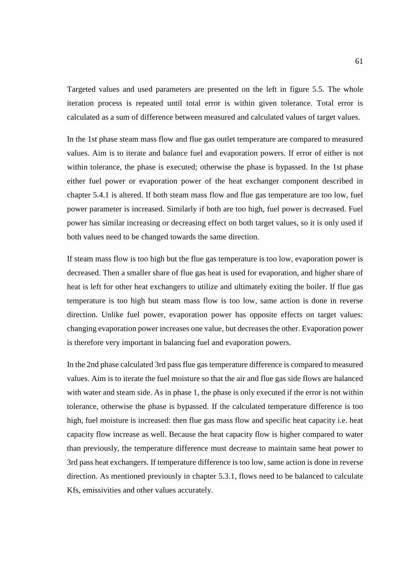
61
Targeted values and used parameters are presented on the left in figure 5.5. The whole
iteration process is repeated until total error is within given tolerance. Total error is
calculated as a sum of difference between measured and calculated values of target values.
In the 1st phase steam mass flow and flue gas outlet temperature are compared to measured
values. Aim is to iterate and balance fuel and evaporation powers. If error of either is not
within tolerance, the phase is executed; otherwise the phase is bypassed. In the 1st phase
either fuel power or evaporation power of the heat exchanger component described in
chapter 5.4.1 is altered. If both steam mass flow and flue gas temperature are too low, fuel
power parameter is increased. Similarly if both are too high, fuel power is decreased. Fuel
power has similar increasing or decreasing effect on both target values, so it is only used if
both values need to be changed towards the same direction.
If steam mass flow is too high but the flue gas temperature is too low, evaporation power is
decreased. Then a smaller share of flue gas heat is used for evaporation, and higher share of
heat is left for other heat exchangers to utilize and ultimately exiting the boiler. If flue gas
temperature is too high but steam mass flow is too low, same action is done in reverse
direction. Unlike fuel power, evaporation power has opposite effects on target values:
changing evaporation power increases one value, but decreases the other. Evaporation power
is therefore very important in balancing fuel and evaporation powers.
In the 2nd phase calculated 3rd pass flue gas temperature difference is compared to measured
values. Aim is to iterate the fuel moisture so that the air and flue gas side flows are balanced
with water and steam side. As in phase 1, the phase is only executed if the error is not within
tolerance, otherwise the phase is bypassed. If the calculated temperature difference is too
high, fuel moisture is increased: then flue gas mass flow and specific heat capacity i.e. heat
capacity flow increase as well. Because the heat capacity flow is higher compared to water
than previously, the temperature difference must decrease to maintain same heat power to
3rd pass heat exchangers. If temperature difference is too low, same action is done in reverse
direction. As mentioned previously in chapter 5.3.1, flows need to be balanced to calculate
Kfs, emissivities and other values accurately.

62
Alternatively to 3rd pass temperature difference method, ratio of water and flue gas heat
capacity flows could be used to iterate fuel moisture. Using temperature difference method
means that flue gas heat capacity flow is compared to both air and water flows. But if water
and flue gas heat capacity flows or their ratio are directly compared, air heat capacity flow
is ignored. In some cases taking air heat capacity flow into account yields more accurate
results, and in other cases it doesn’t. Used condition should be chosen case-by-case, but all
calculations in this thesis are based on the 3rd pass temperature difference method.
In the 3rd phase component outlet temperatures are compared to measured values. Aim is to
iterate heat transfer parameters of each component so that the calculated and measured
temperatures match. As in previous phases, routines are executed only if temperatures aren’t
already within tolerance. The same routine is applied to each heat exchanger individually.
Component iteration routine is described in the next chapter.
In addition to actions shown in the decision tree, smaller adjustments are made every
iteration round. For example, pressure losses are corrected based on measurements and some
mass flows are calculated or assigned.
5.4.4 Component iteration routine
Component iteration routine is done individually for each component. Same solved
parameters are assigned for all components of same type, e.g. all primary LUVO banks have
same Kf and emissivity, but e.g. primary and secondary LUVO banks are iterated separately.
Iteration routine follows decision tree presented in figure 5.6 below.

63
Figure 5.6. Iteration process decision tree for components.
All heat exchangers except for some HSS components follow the same routine presented in
figure 5.6. Routine is executed only if component outlet temperature is not within tolerance,
so based on temperature either Kf or emissivity is changed. As mentioned in chapter 5.2,
emissivity is kept constant if possible to minimize the number of parameters needed to be
configured for new plants. If component outlet temperature is higher than measured and

64
emissivity is higher than recommended initial value, emissivity is decreased. If emissivity is
already equal or lower than recommended value, Kf is decreased. If component outlet
temperature is lower than measured, same actions are done in reverse direction.
After new parameter value is assigned, it is compared to given upper or lower limits. If new
parameter value is higher or lower than the corresponding limit, value is overwritten with
limit value. In case Kf value is overwritten with limit value, emissivity value is increased or
decreased instead. Component iteration routine is applied to each component during the main
iteration process, and it is repeated as a part of the main iteration process until convergence.
5.4.5 HSS iteration routine
HSS iteration routine is done individually for each water – air heat exchangers instead of
component iteration routine introduced in the previous chapter. Unlike other heat
exchangers, water – air heat exchangers aren’t directly connected to other components in the
FB model. Therefore, to help achieve convergence, air outlet temperatures calculated from
HSS components are only used together with other components if they’re within tolerance.
E.g. if calculated air outlet temperature is lower than tolerance allows, the measured value
is used in other components instead. By disconnecting HSS components other than flue gas
– water heat exchanger from the main components convergence is significantly easier to
achieve. Iteration routine follows decision tree presented in figure 5.7 below.

65
Figure 5.7. Iteration process decision tree for HSS water – air heat exchangers.

66
If HSS includes more than one water – air heat exchanger, the same bordered routine
presented in figure 5.7 is executed. Routine is executed only if component outlet temperature
is not within tolerance. Similar to emissivity in component iteration routine, bypass valve
opening is kept constant if possible to minimize the number of parameters needed to be
changed. Bypass valve openings are measured as percentages, and therefore actual mass
flow shares aren’t accurately known. If component air outlet temperature is higher than
measured and opening is lower than recommended initial value, opening is increased. If
opening is already equal or higher than recommended value, UA is decreased. If component
air outlet temperature is lower than measured, same actions are done in reverse direction.
After new value is assigned, it is compared to given upper or lower limits. If new value is
higher or lower than equivalent limit, value is overwritten with limit value. In case UA value
is overwritten with limit value, valve opening value is increased or decreased instead.
If there is a heat exchanger before fans and the temperature rise in fans is not known,
temperature rises are used as parameters. If air outlet temperature is not within tolerance,
temperature rise in fans is either increased or decreased. If new values are outside limits,
they’re overwritten with limit values. Similarly to component iteration routine, HSS iteration
routine is applied to specific components as a part of main iteration process, and repeated
along the main iteration actions until convergence.
5.4.6 Furnace iteration process
Results from converged main iteration process are used to calculate relative burner height
(RBH) in a separate Solvo model. This furnace model is presented in figure 5.8 below.

67
Figure 5.8. Solvo furnace model.
Furnace model presented in figure 5.8 is very simplified and only used for solving RBH. All
fixed parameters are solved in the main iteration process, e.g. mass flows, temperatures and
pressures. On the left from furnace are fuel silo and air inlet components, on the right are
recirculation gas extraction and temperature correction components. Below furnace is water
inlet from steam drum, and above furnace is water and steam outlet to steam drum. On the
top right corner is a required boiler component and two controllers. First controller iterates
FEGT calculated in main iteration process by changing RBH. Second controller iterates air
mass flow calculated in main iteration process by changing air relative humidity.
As a result from this furnace model, RBH corresponding to previously calculated FEGT is
determined. This way the overall iteration of the model is easier, because the evaporation
power as a parameter allows better control over evaporation performance than RBH.
Separate furnace calculation also allows calculating RBH independently which might prove
beneficial, as discussed later in this thesis.

68
5.5 Feedback model limitations and simplifications
Feedback model is designed to iterate detailed information needed in boiler design and
dimensioning process. However, with available online measurements some important
parameters can not be accurately determined.
The performance of different evaporating surfaces is balanced and iterated with only a single
parameter, either RBH or evaporation power. 2nd pass wall correction factor Kf and
emissivity are kept constant, as well as boiler bank parameters. These constant values might
not be accurate, or could depend on the load or other factors. Furnace emissivity inaccuracies
can be compensated with RBH, because both parameters affect the heat transfer
performance. Furnace-component is configured by default to transfer all of its radiation heat
output to furnace walls, but in reality part of the radiation should most likely be allocated to
SH2. This would have an effect on SH2 parameters as well.
2nd pass wall parameters are usually evaporating surfaces and have an effect on heat transfer
surfaces located in 2nd pass. For example, if emissivity of walls in the model is increased, a
higher share of flue gas heat is used for evaporating instead of superheating. Therefore,
accurate wall parameters are important not only in predicting evaporator performance, but
in calculating superheater performance. Similarly, boiler bank parameters are constant,
which affects both evaporator performance and consequently other heat transfer surfaces, as
discussed in chapter 2.5. If boiler bank is estimated to be more efficient than it actually is,
fuel power has to be increased to account for missing evaporating power, which would result
in excessive superheating.
In order to estimate evaporating surface parameters more accurately, additional
measurements should be used. For example, measuring flue gas temperatures before and
after each component would allow determining both component and wall heat powers. This
would also require more accurate measuring methods than typical online measurements, e.g.
suction pyrometers, because the installation errors of online measurements at such
temperatures are generally very high (Andritz 2010, 48-81).
As described for components in chapter 5.4.4, emissivities are kept constant if possible for
all components. Similarly, furnace-component’s emissivity is set to constant. Kf (RBH in

69
furnace-component) is used to account for potentially inaccurate emissivity of each
component, which can yield accurate results for each specific case. However, in future
projects, parameters might not be accurate if e.g. radiative properties of flue gas are not
similar. Determining both correction factor Kf and emissivity experimentally in operating
conditions is most likely not economically feasible.
In addition to Kf and RBH accounting for potential emissivity inaccuracies, fuel moisture is
used to balance air and flue gas side flows with water and steam flows. Calculated fuel
moisture might not always be accurate, and most likely compensates for multiple
inaccuracies, including flue gas temperature and flue gas oxygen content measurement
errors.
Limiting the number of parameters being solved is done to simplify the calculation model
and improve its performance, but also required since with the available measurements some
parameters can’t be determined. Having a low number of parameters that need to be defined
individually also simplifies the design process. Inaccuracies caused by these simplifications
might be significant when designing boiler with untypical fuels or otherwise irregular
conditions.

70
6 RESULTS
Results are discussed in this chapter. Initial conditions are evaluated, calculated process
values compared to measurements, and new, calculated design parameter values introduced.
Results are validated with additional calculations, and results’ reliabilities are discussed.
6.1 Initial conditions and basis for calculations
The reliability and applicability of feedback model results are dependent on the initial
conditions for the calculations. If the measurement data used is not accurate or fuel
significantly differs from assumed, most likely the results will be inaccurate as well. All
calculations are done using feedback model and 3rd pass temperature difference method
described in chapter 5.4. Fuel compositions used are presented in table 6.1 below.
Table 6.1. Fuel compositions used for each case. Light green fuel compositions are based
on fuel analysis, light yellow compositions are based on calculation service approximation,
and the light red compositions are nominal fuel compositions.
Load C H N S O Ash LHV (dry) H2O
[%] [%] [%] [%] [%] [%] [%] [kJ/kg] [%]
Boiler 1
80 46.20 5.40 0.38 0.04 35.18 12.80 17018 49.58
62 50.48 5.90 0.85 0.09 36.31 6.36 19130 49.71
30 49.80 5.77 0.92 0.11 35.71 7.69 18669 38.56
Boiler 2
104 49.96 5.90 0.30 0.02 42.48 1.34 18807 46.86
66 49.96 5.90 0.30 0.02 42.48 1.34 18807 46.86
32 49.96 5.90 0.30 0.02 42.48 1.34 18807 46.86
Boiler 3
101 50.70 6.00 0.35 0.03 40.42 2.50 18961 40.00
61 50.70 6.00 0.35 0.03 40.42 2.50 18961 40.00
33 50.70 6.00 0.35 0.03 40.42 2.50 18961 40.00
Boiler 3 (perf
test)
100 49.80 6.00 0.19 0.02 43.20 0.80 18690 43.40
70 49.80 6.00 0.19 0.02 43.20 0.80 18690 43.40
30 50.10 5.90 0.21 0.02 42.57 1.20 18710 42.20
Boiler 4
100 51.10 5.81 0.61 0.07 39.41 3.00 19370 52.40
59 51.10 5.81 0.61 0.07 39.41 3.00 19370 52.40
34 51.10 5.81 0.61 0.07 39.41 3.00 19370 52.40
Boiler 5 100 50.80 5.90 0.36 0.03 40.91 2.00 18178 44.90

71
According to table 6.1, all fuels are roughly 50 % carbon, and contain about 40 – 50 % water.
The fuel composition is somewhat similar with all boilers except boiler 1, where fuel has
high ash shares and low oxygen shares, and boiler 4, where the fuel has a high heating value.
Initial calculation conditions including measurement period info described in chapter 3.6 are
presented in table 6.2 below.
Table 6.2. Summary of calculation conditions.
Load Measurement
period length Operation point Fuel composition
[%]
Boiler 1
80 4 hours Performance test Fuel analysis
62 19 hours Continuous Calculated approximation
30 >5 days Continuous Calculated approximation
Boiler 2
104 3 days Continuous Nominal fuel
66 6 hours Continuous Nominal fuel
32 8 hours Continuous Nominal fuel
Boiler 3
101 24 hours Continuous Nominal fuel
61 9 hours Continuous Nominal fuel
33 9 hours Continuous Nominal fuel
Boiler 3
(perf test)
100 4 hours Performance test Fuel analysis
70 4 hours Performance test Fuel analysis
30 4 hours Performance test Fuel analysis
Boiler 4
100 1 hour Continuous Nominal fuel
59 8 hours Continuous Nominal fuel
34 2 hours Continuous Nominal fuel
Boiler 5 100 12 hours Performance test Fuel analysis
According to table 6.2, initial conditions for calculations differ case-by-case. Performance
test points for boiler 1, boiler 3, and boiler 5 are the most reliable, because the fuel
composition is based on fuel analysis and the operation conditions have been stable. Fuel
compositions in boiler 1 continuous operation points are based on calculated
approximations, which is a better estimate than nominal fuel, making the points together
with long measurement periods moderately reliable. Fuel compositions in other points are
based on nominal fuels, but boiler 2 and 3 points are still somewhat reliable because of
adequately long measurement periods and quite conventional fuels. Boiler 4 points at high
and low loads are unreliable due to very short measurement periods.

72
6.2 Process values
Process values presented in this chapter are results from FB model that are target values, not
fixed values, in the model. Values are calculated and iterated by changing model parameters.
To estimate the reliability and accuracy of results, calculated process values are compared
to measurements. The most important process values that are not fixed or used as parameters
are presented here.
6.2.1 Mass flows
Steam mass flow is usually one of the main process values of a boiler, and therefore it is
used as one of the main conditions to determine if the model results are converged. Water
and steam mass flow measurements are generally accurate and reliable. Calculated and
measured steam and water mass flows and their differences are presented in table 6.3 below.
Table 6.3. Steam and water mass flows.
Steam mass flow Feed water mass flow
Load Calculated Measured Difference Calculated Measured Difference
[%] [kg/s] [kg/s] [%] [kg/s] [kg/s] [%]
Boiler 1
80 24.01 24.00 0.02 % 24.01 24.00 0.02 %
62 18.55 18.55 0.02 % 18.66 18.66 0.00 %
30 8.85 8.86 0.11 % 9.00 9.00 0.00 %
Boiler 2
104 56.51 56.47 0.07 % 57.20 57.19 0.01 %
66 36.01 36.00 0.04 % 36.01 35.80 0.59 %
32 17.09 17.09 0.03 % 17.79 17.79 0.01 %
Boiler 3
101 20.99 21.00 0.04 % 21.49 21.49 0.00 %
61 12.63 12.64 0.02 % 14.00 14.00 0.01 %
33 6.80 6.80 0.06 % 7.67 7.66 0.08 %
Boiler 3
(perf test)
100 20.70 20.70 0.01 % 20.71 20.71 0.00 %
70 14.60 14.60 0.03 % 15.07 15.07 0.02 %
30 6.48 6.50 0.34 % 7.03 7.03 0.02 %
Boiler 4
96 27.40 27.49 0.32 % 28.18 28.03 0.54 %
59 17.20 17.01 1.12 % 17.88 17.62 1.45 %
34 9.72 9.84 1.19 % 10.09 10.21 1.13 %
Boiler 5 100 42.67 42.68 0.02 % 42.97 42.97 0.00 %

73
According to table 6.3, steam mass flow differences between calculated and measured values
are very low. Feed water mass flows include desuperheater mass flows, and are usually close
to steam mass flows. If feed water mass flow is higher than steam mass flow, part of the
fluid is most likely used for continuous blowdown, sootblowing, or other purpose. The
measured feed water flow for boiler 2 in 66 % load is higher than steam mass flow, which
suggests that either there are inaccuracies in measurements or the boiler hasn’t been in
equilibrium state. For example, water level in steam drum might not have been constant
during the used measurement period. Overall the calculated steam and water mass flows are
close to the measured values, with boiler 4 having slightly higher errors.
Air flow measurements are not usually as accurate as steam or water mass flow
measurements. Measurements shown in this chapter are normal volume flow measurements,
but they are converted to mass flows based on air temperature and moisture. When
calculating a boiler based on measurements, water and gas side mass flows are usually not
completely in balance; therefore, the more reliable water and steam mass flow measurements
are used as target values, and gas side measurements are not. Air mass flows presented here
are used to evaluate the results. Calculated and measured air mass flows and their differences
are presented in table 6.4 below.

74
Table 6.4. Air mass flows.
Primary air mass flow Overfire air flow
Load Calculated Measured Difference Calculated Measured Difference
[%] [kg/s] [kg/s] [%] [kg/s] [kg/s] [%]
Boiler 1
80 15.84 16.80 5.70 % 17.30 18.35 5.70 %
62 11.32 11.11 1.86 % 13.84 13.59 1.86 %
30 9.95 8.94 11.28 % 7.12 6.40 11.29 %
Boiler 2
104 26.94 25.89 4.06 % 46.33 44.52 4.06 %
66 21.13 22.60 6.48 % 25.84 27.63 6.48 %
32 16.92 18.05 6.25 % 13.94 15.59 10.61 %
Boiler 3
101 13.78 13.50 2.05 % 21.14 20.72 2.05 %
61 8.04 7.37 9.20 % 13.67 12.52 9.20 %
33 6.39 6.27 1.91 % 9.97 9.78 1.92 %
Boiler 3
(perf test)
100 11.83 12.31 3.88 % 19.29 20.06 3.88 %
70 9.71 9.96 2.55 % 12.77 13.10 2.53 %
30 4.33 4.47 3.21 % 8.60 8.89 3.20 %
Boiler 4
96 18.28 18.57 1.52 % 22.75 23.10 1.51 %
59 15.78 16.29 3.14 % 10.66 10.98 2.95 %
34 14.13 14.42 1.99 % 3.94 4.02 1.99 %
Boiler 5 100 16.92 18.05 6.25 % 33.48 35.71 6.25 %
According to table 6.4, air mass flow differences are higher than steam and water mass flow
differences presented previously. The ratio of primary and overfire air flows is fixed in the
FB model, and therefore the errors are mostly similar between primary and overfire flows.
Calculated air flows are either higher or lower than measurements depending on the case,
and the errors are 5 – 6 % on average. Differences are relatively low considering the potential
measurement inaccuracies and allowing mass flows to be changed freely in the FB model.
6.2.2 Temperatures
Most target values in FB model are temperatures, and therefore lots of temperature results
are evaluated to determine if the results are converged. Air temperature measurements are
generally not as accurate as steam or water temperature measurements, but they are still used
as target values to calculate LUVO and HSS performance. Calculated and measured air
temperatures and their differences are presented in table 6.5 below.

75
Table 6.5. Air temperatures.
Primary air to boiler temperature Overfire air to boiler temperature
Load Calculated Measured Difference Calculated Measured Difference
[%] [°C] [°C] [%] [°C] [°C] [%]
Boiler 1
80 141.94 142.00 0.04 % 149.95 150.00 0.03 %
62 150.62 150.63 0.01 % 160.96 160.96 0.00 %
30 151.61 151.68 0.05 % 165.94 166.00 0.04 %
Boiler 2
104 230.18 230.20 0.01 % 225.76 225.80 0.02 %
66 206.35 206.45 0.05 % 201.02 201.11 0.04 %
32 163.09 163.16 0.04 % 161.85 161.92 0.04 %
Boiler 3
101 124.93 124.93 0.00 % 124.93 124.93 0.00 %
61 114.32 114.32 0.00 % 114.32 114.32 0.00 %
33 121.77 121.77 0.00 % 121.77 121.77 0.00 %
Boiler 3
(perf test)
100 120.22 120.40 0.15 % 120.22 120.40 0.15 %
70 113.89 113.70 0.17 % 113.89 113.70 0.17 %
30 116.80 116.80 0.00 % 116.80 116.80 0.00 %
Boiler 4
96 151.25 151.33 0.05 % 156.85 156.91 0.04 %
59 147.65 148.43 0.53 % 159.82 161.21 0.86 %
34 143.10 143.56 0.32 % 162.42 163.99 0.96 %
Boiler 5 100 201.23 201.30 0.03 % 240.43 240.50 0.03 %
According to table 6.5, air temperature differences are very low. Due to higher allowed
tolerance in boilers 3 and 4, some differences exist.
Flue gas temperature measurements are fairly accurate if the temperatures are not high. Flue
gas exit temperature together with steam mass flow are important target values in FB model,
used to balance fuel and evaporation powers. Flue gas to 3rd pass temperature is also highly
influential, because it is used to balance fuel moisture and indirectly the balance between
water and gas side flows. Calculated and measured flue gas temperatures and their
differences are presented in table 6.6 below.

76
Table 6.6. Flue gas temperatures.
Flue gas to 3rd pass temperature Flue gas exit temperature
Load Calculated Measured Difference Calculated Measured Difference
[%] [°C] [°C] [%] [°C] [°C] [%]
Boiler 1
80 401.30 401.50 0.05 % 140.90 141.00 0.07 %
62 382.23 382.00 0.06 % 147.75 147.77 0.01 %
30 353.63 353.34 0.08 % 149.15 149.16 0.01 %
Boiler 2
104 417.28 417.49 0.05 % 168.05 168.29 0.14 %
66 368.68 369.04 0.10 % 148.89 149.13 0.16 %
32 421.42 421.20 0.05 % 127.28 127.31 0.02 %
Boiler 3
101 443.57 440.25 0.75 % 152.64 152.14 0.33 %
61 392.17 393.19 0.26 % 139.47 139.27 0.14 %
33 359.31 354.24 1.43 % 135.23 135.02 0.16 %
Boiler 3
(perf test)
100 426.74 424.00 0.65 % 141.71 141.70 0.01 %
70 399.54 387.50 3.11 % 135.95 135.80 0.11 %
30 341.52 335.50 1.79 % 136.96 134.70 1.68 %
Boiler 4
96 423.70 424.56 0.20 % 143.58 144.42 0.58 %
59 390.46 390.31 0.04 % 142.19 143.50 0.91 %
34 358.89 359.42 0.15 % 143.37 143.70 0.23 %
Boiler 5 100 421.42 421.20 0.05 % 146.20 146.20 0.00 %
According to table 6.6, temperature differences are generally low. Again, boilers 3 and 4
have slightly higher differences due to higher allowed tolerance.
Economizer and SH1 outlet temperature measurements are generally accurate and reliable,
and important in determining the performance of said components. Calculated and measured
water and steam temperatures in economizer and SH1 and their differences are presented in
table 6.7 below.

77
Table 6.7. Water and steam temperatures in economizer and SH1.
Eco water outlet temperature SH1 steam outlet temperature
Load Calculated Measured Difference Calculated Measured Difference
[%] [°C] [°C] [%] [°C] [°C] [%]
Boiler 1
80 270.04 270.00 0.01 % 412.05 412.00 0.01 %
62 261.53 261.60 0.03 % 423.17 423.24 0.02 %
30 261.08 261.15 0.03 % 398.55 398.64 0.02 %
Boiler 2
104 310.80 310.77 0.01 % 449.56 449.46 0.02 %
66 278.54 278.62 0.03 % 410.68 410.71 0.01 %
32 267.22 267.27 0.02 % 422.93 422.99 0.01 %
Boiler 3
101 283.15 282.73 0.15 % 402.41 402.26 0.04 %
61 269.10 269.24 0.05 % 393.71 393.87 0.04 %
33 280.01 279.85 0.06 % 379.02 378.76 0.07 %
Boiler 3
(perf test)
100 272.42 272.40 0.01 % 403.37 403.40 0.01 %
70 263.86 262.10 0.67 % 395.09 394.50 0.15 %
30 262.11 266.30 1.57 % 375.83 379.00 0.84 %
Boiler 4
96 274.15 274.10 0.02 % 437.20 436.24 0.22 %
59 258.70 259.21 0.20 % 412.09 413.25 0.28 %
34 251.80 251.75 0.02 % 392.57 390.34 0.57 %
Boiler 5 100 294.01 294.10 0.03 % 405.71 405.80 0.02 %
According to table 6.7, temperature differences are very low. Boilers 3 and 4 have slightly
higher differences than the other boilers.
Similar to economizer and SH1, SH2 and SH3 outlet temperature measurements are accurate
and needed to calculate the components’ performance. Calculated and measured steam
temperatures in SH2 and SH3 and their differences are presented in table 6.8 below.

78
Table 6.8. Steam temperatures in SH2 and SH3.
SH2 steam outlet temperature SH3 steam outlet temperature
Load Calculated Measured Difference Calculated Measured Difference
[%] [°C] [°C] [%] [°C] [°C] [%]
Boiler 1
80 472.01 472.00 0.00 % 510.10 510.00 0.02 %
62 446.04 446.06 0.00 % 465.78 465.79 0.00 %
30 448.19 448.28 0.02 % 467.65 467.73 0.02 %
Boiler 2
104 486.03 485.97 0.01 % 540.14 540.09 0.01 %
66 483.74 483.72 0.01 % 537.44 537.47 0.01 %
32 489.92 490.00 0.02 % 516.36 516.44 0.01 %
Boiler 3
101 445.14 445.00 0.03 % 498.92 498.75 0.03 %
61 437.26 437.44 0.04 % 491.41 491.57 0.03 %
33 430.10 430.02 0.02 % 478.42 478.32 0.02 %
Boiler 3
(perf test)
100 445.32 445.40 0.02 % 499.90 500.00 0.02 %
70 439.51 439.20 0.07 % 500.67 500.00 0.13 %
30 427.94 430.00 0.48 % 479.22 482.50 0.68 %
Boiler 4
96 464.86 464.49 0.08 % 519.93 518.61 0.25 %
59 466.90 464.63 0.49 % 517.04 519.37 0.45 %
34 457.20 456.39 0.18 % 509.25 509.14 0.02 %
Boiler 5 100 489.92 490.00 0.02 % 539.91 540.00 0.02 %
According to table 6.8, temperature differences are very low. Boiler 3 and 4 differences are
slightly higher. Overall, the studied temperature differences are low in all components, and
the results have converged. Due to convergence issues, overall differences in boilers 3 and
4 are higher.
6.3 Design parameters
Design parameters introduced in this chapter are calculated values based on measurement
data and FB model. Calculated values are compared to recommended values. Design
parameter results and potential errors are discussed more carefully later in this thesis.
6.3.1 Relative burner height
Calculated relative burner heights and the average of recommended values are presented in
figure 6.1 below.

79
Figure 6.1. Calculated relative burner heights and average of recommended values.
As shown in figure 6.1, RBH usually increases when the load decreases. RBH in boiler 1
slightly decreases from the medium load to the lowest load, and RBH in boiler 2 is lowest
with the medium load and highest with the lowest load. All the calculated RBH values but
the 80 % load on boiler 1 are higher than recommended values.
6.3.2 Superheaters
Calculated correction factors Kf and recommended values for SH2 are presented in figure
6.2 below. Recommended values are divided to SM (small and medium) and L (large) based
on the size of the boiler.
0
0.1
0.2
0.3
0.4
0.5
0.6
0.7
0.8
20406080100
RB
H
Load %
RBH
Boiler 1
Boiler 2
Boiler 3
Boiler 3 (performancetest)Boiler 4
Boiler 5
Recommended(average)

80
Figure 6.2. Calculated correction factors Kf and recommended values for SH2.
As shown in figure 6.2, SH2 Kf behavior is case-dependent. Kf values are lower than
recommended in most cases. High Kf values in boiler 1 could be due to very high ash content
in the fuel or measurement inaccuracies used in fuel moisture iteration.
Calculated correction factors Kf and recommended value for SH3 are presented in figure 6.3
below.
Figure 6.3. Calculated correction factors Kf and recommended value for SH3.
0.3
0.35
0.4
0.45
0.5
0.55
0.6
0.65
0.7
0.75
0.8
20406080100
Kf
Load %
SH2 Kf
Boiler 1
Boiler 2
Boiler 3
Boiler 3 (performance test)
Boiler 4
Boiler 5
Recommended (SM)
Recommended (L)
0.4
0.5
0.6
0.7
0.8
0.9
1
1.1
20406080100
Kf
Load %
SH3 Kf
Boiler 1
Boiler 2
Boiler 3
Boiler 3 (performance test)
Boiler 4
Boiler 5
Recommended (SM & L)

81
As shown in figure 6.3, SH3 Kf behavior is case-dependent as in SH2. Kf values are
generally higher than the recommended value. High Kf value in boiler 1 at 80% load could
be due to high ash content in fuel. High Kf values at low loads for both boiler 1 and 4 could
be caused by e.g. measurement inaccuracies or inaccurate fuel compositions used.
Calculated correction factors Kf and recommended values for SH1 are presented in figure
6.4 below. Recommended values are divided to SM (small and medium) and L (large) based
on the size of the boiler.
Figure 6.4. Calculated correction factors Kf and recommended values for SH1.
As shown in figure 6.4, SH1 Kf values generally decrease slightly when the load decreases.
Kf values are mostly higher than the recommended value.
Having higher Kf values than recommended means that the surfaces are operating more
efficiently than expected. Since both SH3 and SH1 have significantly higher Kfs than
recommended, but SH2 slightly lower than recommended, the overall superheating should
be higher than expected for most boilers. By adjusting Kf values accordingly, overall
superheater area and material costs could most likely be reduced while still retaining
adequate superheating.
0.5
0.6
0.7
0.8
0.9
1
1.1
20406080100
Kf
Load %
SH1 Kf
Boiler 1
Boiler 2
Boiler 3
Boiler 3 (performance test)
Boiler 4
Boiler 5
Recommended (SM)
Recommended (L)

82
6.3.3 3rd pass
Calculated correction factors Kf and recommended values for economizer are presented in
figure 6.5 below. Recommended values are divided to plain economizer and finned
economizer based on the economizer construction.
Figure 6.5. Calculated correction factors Kf and recommended values for economizer.
As shown in figure 6.5, economizer Kf values generally decrease when the load decreases.
Kf values are mostly close to or higher than the recommended values. Very low Kf value in
boiler 1 at low load is most likely due to measurement inaccuracies or otherwise unreliable
results.
Calculated correction factors Kf and recommended value for LUVOs are presented in figure
6.6 below. Recommended values are divided to SM (small and medium) and L (large) based
on the size of the boiler.
0.4
0.5
0.6
0.7
0.8
0.9
1
20406080100
Kf
Load %
Economizer Kf
Boiler 1 (plain)
Boiler 2 (plain)
Boiler 3 (fin)
Boiler 3 performancetest (fin)Boiler 4 (plain)
Boiler 5 (fin)
Recommended (plain)
Recommended (fin)

83
Figure 6.6. Calculated correction factors Kf and recommended values for LUVOs.
As shown in figure 6.6, LUVO Kf usually increases when the load decreases. Calculated
value for boiler 5 is extremely high, which suggests that the heat transfer area used in
calculations is incorrect or there’s error in temperature measurements.
Calculated correction factors Kf and recommended value for HSS flue gas – water heat
exchanger are presented in figure 6.7 below.
Figure 6.7. Calculated correction factors Kf and recommended value for HSS flue gas – water heat
exchanger.
0.7
0.8
0.9
1
1.1
1.2
1.3
1.4
1.5
20406080100
Kf
Load %
Luvo average Kf
Boiler 1
Boiler 2
Boiler 4
Boiler 5
Recommended (SM)
Recommended (L)
0.5
0.55
0.6
0.65
0.7
0.75
0.8
0.85
0.9
20406080100
Kf
Load %
HSS flue gas - water Kf
Boiler 3
Boiler 3 (performance test)
Boiler 5
Recommended (SM & L)

84
As shown in figure 6.7, calculated HSS Kf values are close to recommended. Value
calculated for boiler 5 is very low, which suggests that the heat transfer area used in
calculations is incorrect or there’s error in HSS air outlet temperature. Air leakage in LUVO
could at least partially explain untypical values in both LUVO and HSS; if the air mass flow
is lower than thought in LUVO but higher in HSS, LUVO Kf would be lower and HSS Kf
would be higher than presented.
6.3.4 Fuel moisture
Initial and calculated fuel moistures, and their absolute differences are presented in table 6.9
below. Initial values are either from fuel analysis, calculated approximations, or nominal
fuel moistures.
Table 6.9. Initial and calculated fuel moistures, and their absolute differences.
Load Initial Difference Calculated
[%] [%] [-] [%]
Boiler 1
80 49.58 -1.09 48.49
62 49.71 -1.477 48.23
30 38.56 14.68 53.24
Boiler 2
104 46.86 12.52 59.38
66 46.86 9.86 56.72
32 46.86 7.71 54.57
Boiler 3
101 40 11.38 51.38
61 40 12.54 52.54
33 40 17.32 57.32
Boiler 3
(perf test)
100 43.4 3.96 47.36
70 43.4 3.92 47.32
30 42.2 3.4 45.6
Boiler 4
100 52.4 3.73 56.13
59 52.4 3.47 55.87
34 52.4 1.17 53.57
Boiler 5 100 44.9 -3.86 41.04
According to table 6.9, differences vary greatly and the moisture values are roughly 40 – 60
%. Initial fuel moistures, apart from performance test cases where moistures are known, are
only assumptions and most likely do not represent the real circumstances. Therefore, only

85
performance test cases should be compared to initial values when estimating result accuracy
or reliability. Calculated boiler 1, 3, and 5 performance test moistures are within 4 % of
analyzed, which is relatively low. Calculated fuel moistures are determined so that the air-
flue gas and water-steam flows are balanced, and therefore they take into account
measurement inaccuracies in e.g. flue gas oxygen content and flue gas temperature
measurements. Additionally, analyzed fuel moistures might not represent the whole
measurement period moisture accurately. Therefore, some error should be expected.
Because fuel moisture is a parameter that is very case specific and usually not known, it is
not as carefully considered when determining accuracy of the results. If fuel moisture from
analyses was directly used in performance test cases, other results would most likely be more
inaccurate.
6.4 Result validation
Results are validated with calculation models separate from the FB model to ensure that they
are reasonable and valid. Calculated parameters are applied to the design model template to
verify their applicability to design purposes, and the calculated furnace exit flue gas
temperatures are compared to a semi-empirical furnace model to estimate result accuracies.
6.4.1 Solvo design template
Calculated parameters, e.g. Kfs, emissivities, and RBH, are calculated with Solvo FB model
that differs from the design model template. To ensure results are valid in Solvo design
models as well, simulations are also conducted with the design template using previously
calculated parameters and only required boundary conditions.
As expected, calculated process values are very close to measurements when using Solvo
design models. There are no controllers or macros in use that would try to adjust parameters
to achieve these values, and therefore, the parameters calculated using FB model are valid
in design process.

86
6.4.2 Furnace exit flue gas temperature
Furnace exit flue gas temperature (FEGT) is not one of the target values, because
temperature measurements in furnace aren’t reliable or accurate. Flue gas temperatures
elsewhere in the boiler are determined by parameters such as fuel moisture, fuel power, and
evaporating power when the iteration is converged. To evaluate these parameters’ accuracy,
FEGT should be validated, since it indicates the overall accuracy of the results.
FEGT is validated with a separate Excel- and Visual Basic –powered furnace model. Furnace
model discussed here is not the same Solvo model that was discussed in chapter 5.4.6. Model
calculates radiative heat transfer and energy balances that are based on flue gas calculations.
Temperature measurements conducted using suction pyrometers on real, operating boilers
are used to both improve the accuracy of the model and validate its results. (Andritz 2010,
48-81)
FEGT is one of the properties that should be considered when choosing the fuel moisture
balancing method discussed in chapter 5.4.3. If the difference between FEGTs calculated
with FB model and furnace model described here is high, alternative method should be
considered or used. Calculated FEGT according to both FB model and furnace model, and
their difference are presented in table 6.10 below. Measured value and difference to FB
model are also presented for reference.

87
Table 6.10. FEGT according to FB model, furnace model, and measurements, and their
differences.
Flue gas exit temperature
Furnace model
(Andritz 2010) Difference FB model Difference Measured
Load
[%] [°C] [%] [°C] [%] [°C]
Boiler 1
80 842.28 0.23 % 844.23 17.20 % 699.00
62 841.97 4.05 % 877.48 22.62 % 679.04
30 634.36 5.51 % 671.36 16.93 % 557.73
Boiler 2
104 992.83 2.02 % 1013.30 19.42 % 816.50
66 895.56 2.21 % 915.81 27.30 % 665.80
32 731.97 0.60 % 736.40 26.68 % 539.90
Boiler 3
101 948.49 3.83 % 913.51 11.00 % 813.01
61 849.35 1.90 % 865.78 11.83 % 763.34
33 700.29 0.02 % 700.40 16.64 % 583.86
Boiler 3
(perf test)
100 948.42 0.98 % 939.22 10.62 % 839.50
70 880.59 4.64 % 923.42 15.04 % 784.50
30 688.63 5.40 % 727.98 25.62 % 541.50
Boiler 4
100 909.36 2.01 % 928.04 21.94 % 724.45
59 812.59 9.07 % 893.61 27.38 % 648.90
34 684.29 18.67 % 841.39 33.24 % 561.73
Boiler 5 100 956.87 1.39 % 970.40 16.46 % 810.70
According to table 6.10, FEGTs calculated with FB model are close to furnace model results.
The average difference is approximately 3.9 %, while the FB model FEGT to measured
FEGT difference is about 20 %. Small errors to furnace model results suggests that the FB
model results are adequately reliable, and furthermore indicates that the continuous
temperature measurements in upper furnace are inaccurate.
Calculated FEGT from FB model is high compared to furnace model in boiler 4 with loads
59 % and 34 %. However, calculated process values are close to measurements. This
suggests that some parameters, e.g. fuel moisture, or some measurements, e.g. flue gas
temperatures, are incorrect. The used measurement period for 34 % load is very short, and
therefore all values might not be in equilibrium state. Regardless of the reason for the
differences, the results should be taken with some reservation.

88
FB model FEGTs are generally slightly higher than furnace model FEGTs. Assuming
furnace model results are more accurate, this suggests that the calculated RBHs are slightly
too high. Higher RBH corresponds to higher FEGT but lower evaporation power in furnace,
so in reality evaporator surfaces after furnace should probably be more inefficient. Then the
furnace evaporation power would have to increase, resulting in lower RBH and FEGT.
Upper furnace water walls, 2nd pass water walls, and BB performance attributes are constant
in FB model, but based on this reasoning they might be lower than expected.
6.5 Result reliability
Summary of differences between calculated values and measurements are presented in table
6.11 below. Also differences between FEGTs from calculations and from the furnace model
introduced in the previous chapter are presented.
Table 6.11. Summary of differences between calculated values and measurements or furnace
model results.
Load Avg mass flow
difference
Avg air and flue
gas ΔT
Avg water
and steam ΔT
FEGT ΔT to
furnace model [%]
Boiler 1
80 2.86 % 0.05 % 0.01 % 0.23 %
62 0.93 % 0.02 % 0.01 % 4.05 %
30 5.67 % 0.04 % 0.02 % 5.51 %
Boiler 2
104 2.05 % 0.05 % 0.01 % 2.02 %
66 3.40 % 0.09 % 0.01 % 2.21 %
32 4.22 % 0.04 % 0.02 % 0.60 %
Boiler 3
101 1.03 % 0.27 % 0.06 % 3.83 %
61 4.61 % 0.10 % 0.04 % 1.90 %
33 0.99 % 0.40 % 0.04 % 0.02 %
Boiler 3
(perf test)
100 1.95 % 0.24 % 0.01 % 0.98 %
70 1.28 % 0.89 % 0.26 % 4.64 %
30 1.69 % 0.87 % 0.89 % 5.40 %
Boiler 4
100 0.97 % 0.22 % 0.14 % 2.01 %
59 2.16 % 0.58 % 0.35 % 9.07 %
34 1.58 % 0.41 % 0.20 % 18.67 %
Boiler 5 100 3.13 % 0.03 % 0.02 % 1.39 %

89
According to table 6.11, on average there are differences in mass flows on all cases.
However, water and steam mass flow differences are very low, and the difference is mostly
from air and flue gas flows. Since the flow measurements for air and flue gas are not as
accurate, they are iterated in the calculation models based on other factors. Therefore, some
difference is expected. Averages of temperature differences between measurements and
calculations are generally insignificant. These values are targeted in the iteration routine, so
in converged calculation results the differences should be low. FEGT values compared to
furnace model are expected to have some differences, because the calculated values are not
targeted to match the furnace model results.
6.5.1 Boiler 1
Boiler 1 cases include a performance test at 80 % load, and continuous operation points with
long measurement periods at 62 % and 30 % loads. Initially, the conditions for the
calculations are good, because the measurements are from stable operation, and the fuel
composition is known in performance test case, and approximated with a calculation service
in continuous operation cases.
Mass flow differences in table 6.11 are small especially for medium (62 %) load, and
adequately small for high and low (80 % and 30 %) load. Differences are mostly from air
and flue gas flows, which can be explained mainly with measurement inaccuracies in flow
measurements. In addition, other factors such as multiple temperature and flue gas oxygen
content measurements ultimately have an effect on the calculated flows. Therefore, in terms
of mass balance, results are reasonably reliable.
Air, flue gas, water, and steam temperature differences are all extremely small, making the
results reliable temperature-wise. FEGT differences to furnace model results are quite low
and similar to other cases and boilers. Based on the temperatures, total heat to water and
steam are calculated accurately and the calculated and measured flue gas exit temperatures
are the same, so the amount of heat extracted from flue gas should be correct. If the FEGTs
are different, the calculated and real heat capacities of flue gas are different as well. On the
other hand, furnace model might not be completely accurate and reliable either, because e.g.

90
the air flows that affect the FEGT are not modeled accurately. Since the differences are quite
small, flue gas heat capacities and the overall results should be reliable.
Boiler 1 design parameters discussed in chapter 6.3 are quite different from other cases,
especially with high and low loads. Superheater Kfs are very high, but economizer and
LUVO Kfs are relatively low. Fuel ash content at high (80 %) load case is very high, 12.8
%, which might explain the untypical parameters at that load. Flue gas with very high ash
content most likely radiates much more prominently than typical, which would increase heat
transfer efficiency especially at high flue gas temperatures, i.e. evaporator and superheaters
(Bahador & Sundén 2008, 2411-2417). Consequently, heat transfer surfaces at low flue gas
temperatures, economizer and LUVO might not be as efficient, hence the lower Kfs. Ash
composition is also influential in radiative properties of flue gas, and could have a significant
effect on the results (Cihan et al. 2018, 25-40).
Even though calculations at high load seem reliable based on the studied target values, some
values can’t be studied because of the lack of measurements. For example, parameters
regarding evaporation powers of 2nd pass walls and boiler bank are kept constant, which
might result in unrealistic values in said components and consequently, in other components
as well. Therefore, as the calculated design parameters are not typical, results are probably
not reliable, but could still be used as indicative values.
With medium (62%) load the design parameters are close to typical, but with low (30%) load
SH2 and SH3 Kfs are high, while LUVO and especially economizer Kfs are low. RBH and
consequently FEGT are quite low as well compared to typical RBH trend. Calculated FEGT
has some difference compared to furnace model, and especially air flows are high compared
to measured values. Calculated fuel moisture seems quite high as well. Flue gas temperature
measurements in boiler 1 are known to be close to walls, which might cause higher
installation error as discussed in chapter 2.6.2. In reality, flue gas temperatures might have
been higher, which in the FB model would decrease the calculated fuel moisture and air
flows. If FB model overestimates the fuel moisture, it tends to calculate hot end less efficient,
and cold end more efficient than they really are. As a result, Kfs at the hot end would have
to be high to compensate for the poor heat transfer efficiency to match the calculated values
to measurements. Similarly, cold end Kfs would be low for the same reasons. In other words,

91
if measurement error exists as suspected, RBH would really be higher, superheater Kfs
would be lower, and 3rd pass Kfs at economizer and LUVO would be higher than presented
at low load. All these changes would shift calculated parameters closer to typical values.
Overall boiler 1 results appear reliable based on mass flows and temperatures, but calculated
design parameters are not typical with high and low loads. High load parameters might be
affected by factors that were not considered during calculations, but they might also be
correct considering the effect of extremely high ash content in fuel. Medium load parameters
are typical and seem reliable, but low load parameters are untypical, which could be caused
by error in flue gas temperature measurements. Design parameters apart from medium load
point should be considered as indicative and not particularly reliable due to these issues.
6.5.2 Boiler 2
Boiler 2 cases include only continuous operation points with adequately long measurement
periods. Nominal fuel is used in all cases, which increases the amount of uncertainty in
calculations. However, the fuels used in boiler 2 are not as diverse as in e.g. boiler 1 and fuel
moisture is iterated, so knowing the fuel composition is not as crucial. Initially, the
conditions for calculations are moderately good, with fuel being the highest source of
uncertainty.
Boiler 2 mass flow differences are reasonable, with air and flue gas flows accounting for
most of the error. Measurement inaccuracies probably account for most of the error.
Temperature differences in air, flue gas, water, and steam are very low, and even calculated
FEGT values are close to furnace model values. Based on process values, results from boiler
2 are reliable.
Calculated design parameters are typical, although on average higher than in other boilers.
Boiler 2 is a large boiler and has higher recommended values to e.g. SH2 and SH1 Kfs than
most of the other boilers, so the higher calculated values are reasonable as well. LUVO Kf
being the lowest at high load is most likely due to LUVO banks that were replaced after the
high load measurement load, but before medium and low load measurement periods.

92
At high load RBH is quite high and SH2 Kf quite low. If RBH was lower in the FB model,
FEGT would be lower and evaporation power of the furnace would be higher.
Simultaneously, SH2 Kf would have to be higher to account for lower flue gas temperatures
near SH2. This could be achieved in the FB model by lowering the performance of
evaporation surfaces after furnace, because the evaporation power of furnace would have to
increase to account for the decreased evaporation power after furnace, thus lowering RBH.
However, since the actual evaporation performance is not measured, results represent the
situation as well as possible with the iterable parameters in use.
Overall boiler 2 results are reliable based on both process values that are close to
measurements, and design parameters that are typical. Most uncertainty comes from the
unknown fuel composition.
6.5.3 Boiler 3
Boiler 3 cases include high, medium, and low loads from both performance tests and
continuous operation points with adequately long measurement periods. Performance test
results are calculated using known fuel compositions, but in continuous operation points
nominal fuel is used, which increases the amount of uncertainty in calculations of said cases.
Initially, the conditions for calculations are good and reliable, with fuel composition being
the highest source of uncertainty in continuous operation points.
Mass flows are close to measured values, with only medium load at continuous operation
having relatively high air and flue gas flow differences. Due to convergence issues higher
tolerance has been allowed, and therefore air, flue gas, water, and steam temperature
differences are higher than normal especially with medium and low loads at performance
test. FEGT differences are relatively low, and typical compared to other boilers. Based on
the process values studied, results are moderately reliable.
Calculated design parameters are in line with other boilers. Calculated RBH values increase
when load decreases, as expected. SH3 and SH1 Kfs with low load at continuous operation
are lower than typical, but otherwise parameters are reasonable. Calculated fuel moisture for
this case is higher than for the other cases of the same boiler, which is usually consistent
with high superheater Kfs as mentioned regarding boiler 1. However, air humidifier together

93
with high fuel moisture and low flue gas temperatures caused by low load might increase
the flue gas moisture to such high levels at such low temperatures, that the heat transfer
properties of flue gas could be better than expected, and consequently the Kf worse.
Overall boiler 3 results and parameters are probably quite reliable based on both process
values that are adequately close to measurements, and the typical design parameters. Low
load case results at continuous operation should be taken with some reservation, and the
values overall with slightly higher uncertainty due to higher allowed tolerances.
6.5.4 Boiler 4
All boiler 4 cases are from continuous operation. Medium load (59 %) measurement period
length is sufficient, but high and low loads (100 % and 34 %) measurement periods are
extremely short. Nominal fuel is used for all cases, which increases the uncertainty in terms
of fuel composition, especially because a wide variety of fuels is used in boiler 4. Initially,
the conditions for calculations are poor and include lots of uncertainties, and the results
should be considered skeptically.
Mass flow differences are quite low, but unlike in most boilers, there are some differences
in water and steam mass flows as well. Similarly to boiler 3, a higher allowed tolerance was
used in iteration to account for high amount of uncertainties. There are some differences in
air, flue gas, water, and steam temperatures as well, but all the differences are within 1 – 2
°C. FEGT differences to furnace model are high with medium and low loads, which suggests
that there are errors in flue gas heat capacities even though the total heat flow to water and
steam is probably correct. Uncertainties in fuel compositions and measurements, such as flue
gas to 3rd pass temperature, could cause significant differences in FEGTs. Based on process
values and especially FEGTs, results at high load are somewhat reliable, at medium load
dubious, and at low load unreliable.
Calculated design parameters are mostly in line with other boilers. RBH increases when load
decreases, as expected, and Kfs are close to other boilers with high and medium loads. With
low load Kfs are relatively high, especially on SH3 and LUVO. Based on FEGT with low
load, these values are most likely not correct.

94
Overall boiler 4 results and calculated design parameters are not reliable. Initial conditions
for calculations include a lot of uncertainties, and with medium load and especially low load
the process value results show inaccuracies. However, calculated parameters are mostly
reasonable apart from few values with low load, and they can be used as indicative values.
6.5.5 Boiler 5
Only a single performance test point at 100 % load from boiler 5 is calculated. Fuel
composition is known and measurement data is steady. Initially, the conditions for
calculations are optimal and reliable.
Mass flow differences are quite low, and practically all the difference is from air flows,
where calculated values are lower than measured. Air, flue gas, water, and steam
temperatures are very close to measured. Calculated FEGT difference to furnace model is
also low. Based on process values, boiler 5 results appear reliable.
Calculated design parameters are not typical compared to other boilers. SH2 and economizer
Kfs as well as RBH are close to typical, but SH3, SH1, and HSS Kfs are low while LUVO
Kf is very high. There is an additional refractory located in the upper furnace that will
increase the superheater performance, which is probably why superheater Kfs are low.
LUVO and HSS Kfs on the other hand are unrealistic; most likely the air temperature
measurement between HSS and LUVO is incorrect, because if the temperature was higher,
both Kfs would be closer to typical.
Overall boiler 5 results are reliable based on process values. However, design parameters are
not typical, which could be caused by both incorrect measurements and the additional
refractory. Therefore, the values should only be used as indicative, because there are no other
results from boilers with upper furnace refractories or other measurement points from the
same boiler to compare the results to.

95
7 DISCUSSION AND CONCLUSIONS
Calculated design parameters are discussed, and new design parameter recommendations are
presented in this chapter. Recommendations for future development and further studies are
discussed as well.
One of the main objectives of this thesis is to improve design accuracy by determining design
parameters based on measurement data. This objective has been achieved if the results are
relied upon. There are uncertainties, but collectively some results show distinct need for
adjusting design parameters, and therefore the design accuracy is improved if the suggestions
in this chapter are applied. Consequently, from having improved design accuracy, the last
objective of creating potential for financial benefits is achieved as well: e.g. adjusting design
parameters on superheaters could reduce material costs. The first objective of implementing
feedback calculations as a part of design process has been achieved through the creation of
the FB model. The model allows feedback calculations relatively easily in the future,
providing valuable data from the delivered boilers.
7.1 Design parameters
Calculated design parameters are somewhat case-dependent and differ from old
recommendations, as discussed in chapter 6.3. Summary of differences between design
parameters compared to recommended values are presented in table 7.1 below. Values are
absolute differences to recommended values, not relative.

96
Table 7.1. Summary of differences between calculated parameters and recommended
values. If calculated parameters are higher than recommendations, differences are positive
and marked with red. If calculated parameters are lower, differences are negative and marked
with blue.
Load Difference to recommended value (Kf)
[%] RBH SH2 SH3 SH1
Plain
eco Fin eco LUVO HSS
Boiler 1
80 -0.041 0.214 0.340 0.290 0.120 - -0.080 -
62 0.207 -0.084 0.126 0.290 0.020 - -0.014 -
30 0.192 0.027 0.340 0.229 -0.306 - -0.101 -
Boiler 2
104 0.307 -0.178 0.151 0.202 0.214 - -0.024 -
66 0.156 -0.137 0.198 0.238 0.196 - 0.004 -
32 0.357 -0.051 0.161 0.219 0.147 - 0.079 -
Boiler 3
101 0.150 -0.060 0.117 0.090 - 0.001 - -0.029
61 0.395 -0.031 0.187 0.085 - 0.023 - -0.032
33 0.517 -0.091 -0.031 -0.043 - 0.018 - 0.055
Boiler 3
(perf
test)
100 0.152 -0.026 0.169 0.179 - 0.027 - -0.005
70 0.338 -0.087 0.121 0.112 - -0.001 - -0.007
30 0.505 -0.135 0.056 0.080 - 0.037 - 0.111
Boiler 4
100 0.055 0.015 0.168 0.290 0.157 - 0.025 -
59 0.218 -0.053 0.199 0.222 0.072 - 0.010 -
34 0.103 -0.121 0.340 0.239 0.042 - 0.193 -
Boiler 5 100 0.123 -0.108 -0.026 -0.054 - -0.041 0.377 -0.176
Average
High 0.124 -0.024 0.153 0.166 0.164 -0.004 0.074 -0.070
Medium 0.263 -0.078 0.166 0.189 0.096 0.011 0.000 -0.020
Low 0.335 -0.074 0.173 0.145 -0.039 0.028 0.057 0.083
All 0.233 -0.057 0.164 0.167 0.074 0.009 0.047 -0.012
Based on values in table 7.1 and the reliability of results discussed in chapter 6.5, general
observations and recommendations can be derived for the design parameters. Calculated
relative burner height (RBH) is higher than recommended in every case but boiler 1 load 80
%, and generally the difference increases when the load decreases.
SH2 correction factor Kf results are lower than recommended in nearly every case. Based
on averages, Kf is closer to recommended at high loads, and lower in medium and low loads.
Calculated SH3 and SH1 Kfs are higher than recommended in nearly every case. The effect

97
of boilers 1 and 4 should be noted in averages: both yield very high values, and their results
are not as reliable as others.
All 3rd pass Kfs are close to recommended values. Calculated plain eco values are slightly
higher than recommended especially at high loads. Fin eco values are very close to
recommended values. LUVO Kfs are higher than recommended at minimum loads, but
otherwise close to recommendations. HSS values are close to recommendations, but similar
to LUVO, calculated Kfs are a bit higher than recommended at minimum loads.
7.2 Recommended values for parameters
Proposed changes to recommended values are presented in table 7.2 below. Values are
absolute differences to old recommended values, but for RBH they represent the proposed
coefficient used with the old RBH equation.
Table 7.2. Summary of old recommended values and proposed changes.
RBH SH2 SH3 SH1 Plain eco Fin eco LUVO HSS
Recommended, S&M 1 0.550 0.650 0.700 0.725 0.675 0.950 0.750
Recommended, L 1 0.600 0.650 0.750 0.725 0.675 1.000 0.750
Change,
conservative
All 1.2 -0.05 0.1 0.1 0.05 0 0 0
High 1.2 -0.02 0.1 0.1 0.1 0 0 0
Medium 1.6 -0.05 0.1 0.1 0.05 0 0 0
Low 2 -0.05 0.02 0.02 0 0.01 0.02 0.05
Change,
aggressive
All 1.6 -0.07 0.12 0.13 0.12 0.01 0.02 -0.01
High 1.6 -0.05 0.14 0.15 0.15 0 0 -0.02
Medium 2.2 -0.07 0.16 0.14 0.09 0.01 0 -0.01
Low 2.5 -0.07 0.06 0.08 0.05 0.02 0.05 0.08
Old recommended values in table 7.2 are divided to S&M and L based on the size of the
boiler. Changes to recommended values are divided to conservative and aggressive, and to
single values, “All” and load-dependent values “High”, “Medium”, and “Low”.
Conservative changes are smaller and yield closer values to old recommended values than
aggressive changes that are closer to calculated values. Single values can be applied to all
loads, but load-dependent values apply based on the boiler steam load.

98
Recommended values for both RBH and correction factor Kf have been constant for all
loads. However, based on feedback calculation results, especially RBH is distinctly load-
dependent. In addition, to some extent all Kf values are load-dependent as well. Therefore,
adopting load-dependent values is recommended where applicable. Single, constant values
usually represent 100 % loads fairly well, and proposed changes to constant values are
chosen accordingly, if load-dependent values are not adopted.
Boilers 2 and 3 are the most influential in determining the new recommendations, while
boilers 1, 4, and 5 results are mostly indicative and used for reference. Conservative
recommendations are chosen so that the new values for RBH and Kfs would yield process
values that are closer to real, measured values, but at the same time the changes would be
reasonably safe and small to implement without encountering unexpected phenomena or
having the risk of making too large adjustments. Aggressive recommendations would yield
process values that are even closer to calculated values, but the changes could potentially be
too large, which could lead to unexpected issues. New recommended values would still be
between old recommended values and calculated values, so if the calculation results are
accurate, aggressive changes could enable much more accurate design and better results than
conservative changes.
Recommended changes for RBH are approximate coefficients to original RBH equation,
where the equation results should be multiplied with given coefficients based on the load in
question. Ultimately the equation should be revised so that the load is one of the variables.
Coefficient or the equation results should increase when load decreases.
Most recommended changes to Kfs are increases, which applies to SH3, SH1, economizer,
LUVO and with low loads to HSS. The magnitudes of recommended changes are highest
for SH3 and SH1, where Kfs should be increased by about 0.1 – 0.13 on average. Changes
should be higher for high and medium loads, and smaller for low loads. Plain eco Kf should
be increased quite significantly as well, 0.05 – 0.12 on average. Increases should be highest
at high loads. Calculated fin eco Kf values are very close to recommended values, so they
don’t necessarily need to be adjusted. Medium and low loads Kf could be increased slightly,
about 0.01 – 0.02. LUVO and HSS Kf values are close to recommended as well, but
especially with low loads the Kf values should be increased, about 0.02 – 0.05 and 0.05 –

99
0.08 respectively. Having conservatively low Kf values in 3rd pass might serve as error
margins in some guarantees, such as efficiency or flue gas exit temperature.
SH2 is the only surface where the Kfs should clearly be decreased. Changes should be about
-0.05 – -0.07 on average, where the magnitude should be slightly smaller with high loads,
and greater with low loads. HSS Kf at high and medium loads should also be decreased
slightly.
Due to limited amount of reliable calculation results, conservative changes are
recommended. When the number of calculated points increases in the future, more
aggressive changes could be carried out if needed. RBH changes should definitely be load-
specific, but for Kfs single values for all loads could be adequate until more calculation
points are available. Alternatively, single value recommendations could be used for high and
medium loads, but since low load recommendations are quite different from single values,
applying load-dependent values for low loads might be reasonable.
7.3 Future development
Current state of the feedback model is applicable and functional for most boiler
configurations, and therefore could be added to pre-existing design tools fulfilling one of the
main objectives of this thesis, implementing feedback calculations to design process.
However, further development is needed to improve the ease of use and the calculation
performance of the model.
Currently, measurement data is entered to a separate Excel-workbook, where selected values
are exported to Solvo. Solvo is used to iterate until convergence, and the results are imported
back to Excel. Some additional adjustments might need to be done in Solvo during
calculations. To simplify the calculation process, basic information could be fetched from
elsewhere in the design tools automatically. Similarly to design process, iteration should
preferably be done from Excel or the design tools, so that the user wouldn’t have to be
concerned about Solvo usage.
As mentioned previously, some convergence issues have occurred with boilers 3 and 4,
requiring higher allowed tolerances. Iteration routine should be adjusted and improved so

100
that convergence is easier to achieve, and divergence can be better avoided. This could be
achieved by identifying and altering components where amplitude of process values between
iteration rounds is high. Adjusting iteration coefficients and step sizes of the overall process
and individual components might help as well. For example, desuperheaters have been noted
to not always work as intended, and alternative setups should be studied. Improving
convergence and avoiding divergence would not only yield more accurate results, but ease
the use of the model.
Calculation performance, rate of convergence, and the overall speed of calculation process
could be improved by adjusting the iteration coefficients. At current state, the coefficients
i.e. magnitudes of change in parameters between iteration rounds is proportional to the
difference between the calculated value and the target value i.e. the measured value.
However, by considering additional factors, such as the gradients of the target value,
convergence might be achieved significantly faster (Kelley 1995). Considering the iteration
history of parameters and target values, or the effect of parameter on other process values
more carefully would also speed up the process. Overall, the iteration routine basics seem
functional and efficient, but the model requires more fine-tuning.
7.4 Further studies
Design parameters can already be adjusted based on the first feedback model calculation
results, but for more accurate, reliable, and additional results more calculations or studies
should be carried out. Most importantly, calculating more points with different loads and
boilers will improve the reliability and accuracy of the parameters.
As discussed in chapter 5.5, calculating evaporating powers of upper furnace, 2nd pass walls,
and boiler bank requires additional measurements. As in the furnace model used for
validation, e.g. suction pyrometers could be used to conduct measurement campaigns, where
the temperature measurements would be accurate and done preferably between each
component (Andritz 2010, 48-81). Alternatively, e.g. acoustic temperature measurements
even as continuous measurements might be viable if applicable references are available
(Tian et al. 2018, 1-6). Better measurements would enable calculating evaporator surface
parameters, and thus further improve the accuracy of the feedback model.

101
Based on the calculated design parameters and new recommendations discussed previously,
load-dependency has been observed not only in RBH, but in most of the Kfs. At the current
version of the feedback model emissivities are constant nearly always. However, adjusting
emissivities might decrease the load-dependency. Having lower constant furnace emissivity
would require lower RBH values to satisfy the needed evaporation powers. Additionally due
to temperatures, lowering emissivity would most likely affect lower load RBH values more,
because the temperatures and more prominently, radiative heat powers, would be lower as
well. For similar reasons, adjusting emissivities in different components might decrease the
load-dependency as well. Emissivities’ effect on the design parameters should be studied to
see if radiative heat transfer is the reason for Kf values’ load-dependency, and if by adjusting
emissivities constant Kf values could be used.
Separate Solvo furnace model discussed in chapter 5.4.6 can be used independently without
the main feedback model. Together with furnace model discussed in chapter 6.4.2, RBH
values could be determined as a function of fuel power with low amount of measurements.
This could be utilized to determine a large amount of RBH values from different boilers with
lower effort than by calculating the whole boilers with feedback model. Since RBH is the
most important parameter out of all individual parameters, more reliable RBH equations or
correlations could be formed using this approach.

102
8 SUMMARY
The motivation for this thesis and for developing the feedback model was to receive feedback
and improve accuracy in boiler process design. Based on the thesis subject, three main
objectives were formed: allowing implementation of feedback calculations to design process
and project follow-up, improving boiler dimensioning accuracy and thus reducing error
margins and enabling tighter guarantees, and finally, creating potential to achieve financial
benefits from more accurate boiler design process.
The first objective of this thesis is fulfilled, because a functional feedback model was
developed, and the model could already be implemented in design software. However,
further development on especially the ease of use and the convergence behavior is strongly
recommended before any extensive additional calculation campaigns are conducted. The
second objective of improving boiler dimensioning accuracy is most likely achieved if
suggested changes to recommended values are applied. Overall accuracy can be further
improved and be more relied upon with more calculated cases. The third objective is partly
dependent on the second objective being achieved, but also on having more information and
feedback about the delivered boilers. Based on this thesis second objective is achieved if the
results are correct, and therefore there is also potential for achieving financial benefits, which
conditionally fulfills the third objective.
At the start of this thesis steam generation and BFB boiler basics were discussed. The theory
basis for further discussion regarding measurements and heat transfer was described. Studied
boilers and pre-existing boiler models were introduced. The principles and methodology of
the developed feedback model including multiple iteration approaches were evaluated and
described. Initial conditions for boilers differed greatly due to available measurement data,
operation conditions, boiler properties, and multiple other factors.
Feedback calculation results indicated that the previous recommended design parameter
values were not always accurate. Process values close to measured were achieved using the
feedback model, but the parameters required to achieve those values were, for a lot of
components, different than the recommendations. Calculations were validated with e.g. a
separate, semi-empirical furnace model. The reliability of results varied case-by-case, but

103
based on the most reliable results and the most noticeable differences, new parameter values
were suggested.
The feedback model should be further developed to improve its convergence behavior and
ease of use. At current state operation of the model might require a lot of expertise in the
simulation software and the model itself. Further studies should be conducted to estimate the
effects of emissivities, to calculate higher volume of RBH values, and to first and foremost,
have more results and data to improve model results’ reliability. The recommended
parameter values should increasingly shift from the old values towards the calculated values
when the amount of data and reliability increases as well.

REFERENCES
Andritz. 2010. 1D Furnace Model. [Internal material]
Andritz. 2014. Sootblowing system. [Internal material]
Andritz. 2015. Introduction. [Internal material]
Andritz. 2017a. Ash handling. [Internal material]
Andritz. 2017b. Solid fuel and bed material feeding. [Internal material]
Andritz. 2018. Combustion air system. [Internal material]
Andritz. 2020a. Heat shift system (Cyclex). [Internal material]
Andritz. 2020b. Selected References – Biomass Boilers. [Internal material]
Bahador, M. & Sundén, B. 2008. Investigation on the effects of fly ash particles on the
thermal radiation in biomass fired boilers. International Journal of Heat and Mass Transfer,
vol. 51, pp. 2411-2417.
Basu, S. & Debnath, A. K. 2014. Power Plant Instrumentation and Control Handbook: A
Guide to Thermal Power Plants. London: Elsevier Science & Technology. ISBN 978-0-12-
800940-6.
Cihan, A., Nevin, S. & Gorkem, K. 2018. Influence of fly ash composition on non-gray
particle radiation in combusting systems. Journal of Quantitative Spectroscopy and
Radiative Transfer, vol. 215, pp. 25-40.
EN 12952-15. 2003. Water-tube boilers and auxiliary installations – Part 15: Acceptance
tests. European Committee for Standardization. Brussels.
Finnish Environment Institute. 2001. Finnish Expert Report on Best Available Techniques
in Large Combustion Plants. The Finnish Environment 458. Helsinki: Edita Oyj. ISBN 952-
11-0861-4.

Fortum. 2020. Solvo [web brochure]. [Accessed 10.6.2020]. Available:
https://www.fortum.com/sites/default/files/documents/solvo_en.pdf
Huhtinen, M., Kettunen, A., Nurminen, P. & Pakkanen, H. 2004. Höyrykattilatekniikka
(Steam boiler technology). 6th ed. Helsinki: Edita Prima Oy. ISBN 951-37-3360-2 (in
Finnish).
Huhtinen, M., Korhonen, R., Pimiä, T. & Urpalainen, S. 2008. Voimalaitostekniikka (Power
plant technology). Keuruu: Opetushallitus. ISBN 978-952-13-3476-4 (in Finnish).
Hutter, K. & Wang, Y. 2016. Fluid and Thermodynamics Volume 1: Basic Fluid Mechanics.
Advances in Geophysical and Environmental Mechanics and Mathematics. Switzerland:
Springer International Publishing. ISBN 978-3-319-33632-9.
Incropera, F. P. & DeWitt D. P. 2002. Fundamentals of Heat and Mass Transfer. 5th ed. NJ,
USA: John Wiley & Sons, Inc. ISBN 0-471-38650-2.
Kelley, C. T. 1995. Iterative Methods for Linear and Nonlinear Equations. Philadelphia:
Society for Industrial and Applied Mathematics. ISBN 9780898713527.
Moran M. J. & Shapiro H. N. 2002. Fundamentals of Engineering Thermodynamics. 3rd ed.
Chichester: John Wiley & Sons Ltd. ISBN 0-471-97960-0.
Motiva. 2011. Opas höyryn ja lauhteen siirtojärjestelmien energiatehokkuuden mittaamiseen
(Guide to measuring energy efficiency of steam and condensate transportation systems) [web
article]. [Accessed 12.6.2020] (in Finnish). Available:
https://www.motiva.fi/ajankohtaista/julkaisut/kaikki_julkaisut/opas_hoyryn_ja_lauhteen_si
irtojarjestelmien_energiatehokkuuden_mittaamiseen.9236.shtml
Raiko, R., Saastamoinen, J., Hupa, M. & Kurki-Suonio, I. 2002. Poltto ja palaminen (Firing
and combustion). Jyväskylä: International Flame Research Foundation. ISBN 951-666-604-
3 (in Finnish).
Solvo. 2020. Design components [user manual]. [Accessed 12.6.2020].

Tian, F., Zhang, H. & Tian, Y. 2018. Design and implementation of furnace temperature
measurement system for power plant coal-fired boiler in acoustic method. MATEC Web of
Conferences, vol. 232.
Vakkilainen, E. K. 2017. Steam generation from biomass: Construction and Design of Large
Boilers. Amsterdam: Butterworth-Heinemann. ISBN 978-0-12-804389-9.
Vattenfall AB. 2020. ChlorOut [website]. [Accessed 10.6.2020]. Available:
https://group.vattenfall.com/what-we-do/business_model/chlorout
VDI-Gesellschaft Verfahrenstechnik und Chemieingenieurwesen (ed.). 2010. VDI Heat
Atlas. 2nd ed. Berlin: Springer-Verlag. ISBN 978-3-540-77876-9.
Weiss, J. 1993. More accurate sensors needed to reduce uncertainty. Power Engineering,
vol. 96, pp. 29-32.


