Download - Use of Stable Carbon and Nitrogen Isotopes to Trace the Larval

Use of Stable Carbon and Nitrogen Isotopes to Trace the Larval Striped Bass Food Chain in the Sacramento-San Joaquin Estuary, California, April to September 1985

By Walter RastU.S. GEOLOGICAL SURVEYand

James E. SuttonCALIFORNIA STATE WATER RESOURCES CONTROL BOARD

U.S. GEOLOGICAL SURVEY Water-Resources Investigations Report 88-4164

Prepared in cooperation with theCALIFORNIA STATE WATER RESOURCES CONTROL BOARD

Sacramento, California 1989

DEPARTMENT OF THE INTERIOR

MANUEL LUJAN, JR., Secretary

U.S. GEOLOGICAL SURVEY

Dallas L. Peck, Director

For additional information write to:

District Chief U.S. Geological Survey Federal Building, Room W-2234 2800 Cottage Way Sacramento, CA 95825

Copies of this report may be purchased from:

U.S. Geological SurveyBooks and Open-File

Reports SectionBox 25425Building 810, Federal CenterDenver, CO 80225

CONTENTS

PageAbstract .................................................................. 1Introduction .............................................................. 2Analysis of aquatic food chains using stable isotopes ..................... 4

Stable isotopes and food chains ...................................... 4Calculation of stable isotope ratios ................................. 5

Study methods ............................................................. 6Field collection of samples .......................................... 6

Small particulate matter ........................................ 8Particulate organic matter <43 ym (phytoplankton) .......... 9Particulate organic matter >43 ym (small zooplankton) ...... 9

Large zooplankton ............................................... 9Detritus, Neomysis shrimp, and larval striped bass .............. 10Municipal wastewater-treatment plant effluents .................. 10

Laboratory analysis of samples ....................................... 10Detritus ........................................................ 10Particulate organic matter <43 ym (phytoplankton) ............... 11Particulate organic matter >43 jam (small zooplankton) ........... 11Large zooplankton ............................................... 11Neomysis shrimp ................................................. 12Larval striped bass ............................................. 13Municipal wastewater-treatment plant effluents .................. 13Measurement of stable isotope ratios ............................ 13

Stable carbon and nitrogen isotope ratios ................................. 14Detritus ............................................................. 16Particulate organic matter <43 ym (phytoplankton) .................... 17Particulate organic matter >43 ym (small zooplankton) ................ 19Large zooplankton .................................................... 19Neomysis shrimp ...................................................... 21Larval striped bass .................................................. 22Municipal wastewater-treatment plant effluents ....................... 24

Carbon and nitrogen flux between trophic levels ........................... 25Temporal and spatial variations ........................................... 32

Mean isotope ratios by sampling site ................................. 33Mean isotope ratios by sampling date ................................. 34Mean isotope ratios for specific study components .................... 36

Detritus ........................................................ 36Particulate organic matter <43 ym (phytoplankton) ............... 37Particulate organic matter >43 ym (small zooplankton) ........... 39Large zooplankton ............................................... 40Neomysis shrimp ................................................. 42

Mean isotope ratios at individual sampling sites ..................... 43Future research needs ..................................................... 44Summary and conclusions ................................................... 45References cited .......................................................... 48

Contents III

ILLUSTRATIONS

Page Figure 1. Map showing location of study area and data-collection

sites in the Sacramento-San Joaquin Estuary .................. 32-17. Graphs showing:

2. Grand mean stable carbon and nitrogen isotope ratios andstandard deviations for study components ................ 26

3. Mean stable carbon and nitrogen isotope ratios and standard deviations for detritus, POM <43 ym (phytoplankton) and POM >43 ym (small zooplankton) ...... 29

4. Mean stable carbon isotope ratios, by site ................ 335. Mean stable nitrogen isotope ratios, by site .............. 346. Mean stable carbon isotope ratios, by date ................ 357. Mean stable nitrogen isotope ratios, by date .............. 358. Mean stable carbon isotope ratios for detritus ............ 369. Mean stable nitrogen isotope ratios for detritus .......... 37

10. Mean stable carbon isotope ratios for POM <43 ym(phytoplankton) ......................................... 38

11. Mean stable nitrogen isotope ratios for POM <43 ym(phytoplankton) ......................................... 38

12. Mean stable carbon isotope ratios for POM >43 ym (smallzooplankton) ............................................ 39

13. Mean stable nitrogen isotope ratios for POM >43 ym (smallzooplankton) ............................................ 40

14. Mean stable carbon isotope ratios for large zooplankton ... 4115. Mean stable nitrogen isotope ratios for large zooplankton 4116. Mean stable carbon isotope ratios for Neomysis shrimp ..... 4217. Mean stable nitrogen isotope ratios for Neomysis shrimp ... 43

TABLES

Page Table 1. Sampling dates and sites for which data were obtained ........... 7

2. Summary of grand mean stable carbon and nitrogen isotoperatios ........................................................ 15

3. Mean stable carbon and nitrogen isotope ratios fortwo groupings of striped bass ................................. 23

4. Mean stable carbon and nitrogen isotope ratios formunicipal wastewater-treatment plant effluents ................ 25

5. Alternative lines-of-best-fit for striped bassfood chain components ......................................... 27

6. Stable carbon isotope ratios for detritus ....................... 507. Stable nitrogen isotope ratios for detritus ..................... 518. Stable carbon isotope ratios for POM <43 ym (phytoplankton) ..... 529. Stable nitrogen isotope ratios for POM <43 ym (phytoplankton) ... 53

IV Contents

Page Table 10. Stable carbon isotope ratios for POM >43 ym (small

zooplankton) ................................................. 5411. Stable nitrogen isotope ratios for POM >43 ym (small

zooplankton) ................................................. 5512. jStable carbon isotope ratios for large zooplankton ............. 5613. Stable nitrogen isotope ratios for large zooplankton ........... 5714. Stable carbon isotope ratios for Neomysis shrimp ............... 5815. Stable nitrogen isotope ratios for Neomysis shrimp ............. 5916. Stable carbon isotope ratios for striped bass .................. 6017. Stable nitrogen isotope ratios for striped bass ................ 6118. Stable carbon isotope ratios for municipal wastewater-

treatment plants ............................................. 6219. Stable nitrogen isotope ratios for municipal wastewater-

treatment plants ............................................. 62

CONVERSION FACTORS

Metric (SI) units are used in this report. For readers who prefer inch/pound units, the conversion factors for the terms used in this report are listed below:

Multiply

cm (centimeter)g (gram)L (liter)m (meter)ym (micrometer)mm (millimeter)

By

0.39370.035270.26423.2810.000039370.03937

To obtain

inchounce (avoirdupois)gallon (U.S. liquid)footinchinch

Temperature is given in degrees Celsius (°C), which can be converted to degrees Fahrenheit (°F) by the following equation:

°F=1.8(°C)+32.

Isotope composition is expressed in parts per thousand or "per mil."

Other Abbreviations Used:

hmin mg o/oo

hour minute -milligram per mil

Conversion Factors V

Use of Stable Carbon and Nitrogen Isotopes to Trace theLarval Striped Bass Food Chain in the Sacramento-

San Joaquin Estuary, California, April to September 1985

By Walter Rast and James E. Sutton1

The economically and recreationally important striped bass fishery in the Sacramento-San Joaquin Estuary, California, has been experiencing a continuing decline in recent decades. One hypothesis for this decline is that one or more lower trophic-level components of the striped bass food chain have decreased in numbers, or that the lower end of the food chain trophic structure has been otherwise disrupted. This has resulted in an insufficient food supply for striped bass during their larval stage, which has affected the entire striped bass food chain, resulting in decreasing numbers of adult striped bass. To examine this hypothesis, a study was conducted in late spring and summer of 1985, during the striped bass spawning season. The ratios of the stable isotopes of carbon and nitrogen in the organic components of the presumed food chain were used as a tracer to examine the flux of these elements as one progresses through the striped bass food chain. A primary goal of this analysis was to examine the trophic structure of the lower and middle levels of the presumed striped bass food chain.

The results of this study generally confirm a larval striped bass food chain in the Sacramento-San Joaquin Estuary consisting of the elements, phytoplankton/detritus >zooplankton/#eomysis shrimp >striped bass. No unusual trophic structure was found. However, the stable isotope data indicate the possibility of an unidentified, unsampled consumer organism occupying an intermediate position between the lower (phytoplankton, small zooplankton, organic detritus) and upper (large zooplankton, Neomysis shrimp) trophic levels of the striped bass food chain. This unidentified consumer would have a stable carbon isotope ratio of about -28 per mil and a stable nitrogen isotope ratio of about 8 per mil. The stable isotope data also indicate the position of phytoplankton, small zooplankton, and organic detritus at the lower end of the food chain. Owing to the similarity of their stable isotope ratios, these three components were grouped together as one component for this study.

The data also indicate three possible feeding stages for larval striped bass, depending on the length of the fish. The smallest length striped bass subsist on the remnants of their yolk sacs, and the larger length striped bass subsist on Neomysis shrimp and large zooplankton. The intermediate length striped bass seem to represent a transition stage from one primary food source to another and (or) a mixture of food sources. The specific food sources during this transition stage likely are dependent in part on the relative sizes of the striped bass and their potential prey organisms in the striped bass spawning area, as well as their relative abundance.

1James E. Sutton, California State Water Resources Control Board, .Sacramento, California.

Abstract 1

INTRODUCTION

Striped bass (Morone saxatilis) were introduced into the Sacramento-San Joaquin Estuary, California, in the late 1800's, and the population increased significantly into the early 1900's. The number of striped bass remained stable following a commercial fishing ban in 1935, until about the mid-1960's when an erratic, but continuing decline occurred in the numbers of striped bass in the estuary. The adult population of striped bass in recent years is only about one-fourth of the population observed in 1965. Furthermore, the present production of juvenile striped bass is significantly lower, at only about one- third to one-half of the predicted level based on a model of striped bass abundance (Stevens and others, 1985).

The California Department of Fish and Game has measured the abundance of juvenile striped bass in the Sacramento-San Joaquin Estuary (fig. 1) annually since 1959. Based on biweekly sampling conducted from spring to mid- to late summer, the Department of Fish and Game calculates an annual striped bass index. Historically, this index has served as a measure of the general state of the striped bass fishery. Data collected between 1959 and 1982 indicate that the striped bass index for Suisun Bay and for the estuary in general has been declining steadily since about the mid-1960's (Striped Bass Work Group, 1982).

The striped bass fishery in the Sacramento-San Joaquin Estuary, Califor nia, represents an economically and recreationally important fishery for this region. Because of the significant decline of striped bass in this fishery in recent years, the California State Water Resources Control Board organized a Striped Bass Work Group in 1982. This work group was organized to examine the extent of the decline of the striped bass fishery, to attempt to identify the potential causes of the decline, and to develop recommendations for possible corrective actions. The interagency Striped Bass Work Group consisted of scientists from the University of California at Davis, California Department of Water Resources, California Department of Fish and Game, U.S. Bureau of Recla mation, U.S. Fish and Wildlife Service, and the National Marine Fisheries Ser vice, as well as consultants from Kelley and Associates, Envirosphere, and Ecological Analysts.

The Striped Bass Work Group (1982) concluded, among other possibilities, that the decline in the striped bass fishery might be due to an inadequate food supply during the larval stage of striped bass. This possibility is based on the striped bass food chain as fisheries scientists believe it exists in the Sacramento-San Joaquin Estuary. Simplified, this food chain can be approxi mated as having the trophic structure, phytoplankton/detritus >zooplankton/ Neomysis shrimp >striped bass.

The results of zooplankton population surveys in waters of the Sacramento- San Joaquin Estuary are consistent with the possibility of an inadequate food supply (through the food chain) for larval striped bass. The decline of striped bass and zooplankton also coincided with a general decline in phytoplankton in the estuary. Because phytoplankton and organic detritus are believed to con stitute a significant part of the zooplankton diet, the Striped Bass Work Group suggested that the significant decline in the striped bass fishery may have been related to a disturbance of the lower trophic level of the striped bass food chain.

2 Striped Bass Food Chain, Sacramento-San Joaquin Estuary, California

38°30V122°30' 121° 30'

Sacramento municipal wastewater-treatment

plant

STUDY AREEU&EL13A

CARQUINEZ STRAIT

Benicia

StocktorKfliunicipal wastewateNreatment

lant. ,<£CliftonCourt

Forebay

EXPLANATIONSTUDY AREA

San FranciscoSAMPLING SITE

PUMPING PLANT

0 100 200 KILOMETERS

FIGURE 1.-Location of study area and data-collection sites in the Sacramento-San Joaquin Estuary.

Theoretically, an energy (food) flow from the lower trophic levels (phytoplankton/detritus) to the higher trophic levels (zooplankton/Weomysis shrimp) of the food chain is required to maintain the striped bass fishery. Thus, the purpose of this investigation was to determine whether a disruption of any component in the food chain may have occurred between the lower and higher trophic levels of the food chain. This report presents the results of this investigation. Samples of organisms from all identified trophic levels of the striped bass food chain were collected at four sites from April to Septem ber 1985. Stable isotope ratios were used to assess the flux of nitrogen and carbon from the lower trophic levels to the higher trophic levels of the striped bass food chain.

Introduction 3

This study was done by the U.S. Geological Survey in cooperation with the California State Water Resources Control Board and was financed (in part) with Federal funds from the U.S. Environmental Protection Agency under grant number C060000-21. The contents do not necessarily reflect the views and policies of the Environmental Protection Agency or the California State Water Resources Control Board. The assistance of many individuals of the California Department of Fish and Game is gratefully acknowledged. The able assistance of Greg Schmidt in collecting the necessary samples, and of Lee Miller, Alice Fusfeld Low, and Don Stevens in providing technical information and guidance regarding the spawning and feeding habits of striped bass, was especially helpful in the completion of this study.

ANALYSIS OF AQUATIC FOOD CHAINS USING STABLE ISOTOPES

Stable Isotopes and Food Chains

The use of stable isotopes for analysis of food chains is based on the concept that "one is what one eats." Thus, one can attempt to assess the food chain relations of higher trophic level organisms by examining their presumed food sources, which commonly are organisms at lower trophic levels (DeNiro and Epstein, 1978; Rau and others, 1981; Fry and Sherr, 1984). The use of stable isotopes to make this assessment is based on the fact that all elements (including carbon and nitrogen) have a number of isotopic forms. In addition, the isotopic composition of most organic matter (including living organisms) is controlled by a few key chemical and physical reactions. In the photosynthesis reaction of plants, for example, there is a preferential selection of the stable carbon isotope, 12C, relative to the slightly heavier 13C isotope, due to a kinetic isotope fractionation that occurs during the photosynthesis reaction (Park and Epstein, 1961). This results in an enrichment of the plant cellular material with the lighter isotope. Such isotopic fractionation in plants can be passed on to higher trophic level organisms (predators for the lower trophic level organisms) with little change. This isotopic fractionation can occur even though normal biochemical processes may significantly alter other components in the cell (Fry and Sherr, 1984).

The same phenomenon is applicable to predator-prey food chains. Thus, although the stable carbon isotope ratio of a predator organism will closely resemble its food source, one usually would see a small but significant positive increase in the ratio of the predator organism. In various studies, consumer organisms show a stable carbon isotope ratio of about 1 o/oo more positive than the organisms on which they feed. Consumer organisms usually have stable nitrogen isotope ratios about 3 o/oo more positive than those of their food sources. This enrichment occurs at each transfer of energy (carbon) from one trophic level to the next highest trophic level, although there are some exceptions to this rule (Rau and others, 1983; Gearing and others, 1984; Fry and Sherr, 1984). Thus, ideally, one would expect to see an increase of about 1 o/oo for stable carbon isotopes and 3 o/oo for stable nitrogen isotopes for each transfer of energy from a lower trophic level to the next highest trophic level in a food chain. This small increase should continue in a progressive manner as one proceeds from prey organisms at the bottom of a food chain to predator organisms at the top of a food chain (Rau and others, 1983; Fry and Sherr, 1984; Peterson and others, 1985).

4 Striped Bass Food Chain, San-Joaquin Estuary, California

Because of this property, the ratio of the stable isotopes in the cellular components of higher trophic level organisms often can be used to study the origins and transformations of the organic matter comprising the organisms. Measurement of stable carbon and nitrogen isotope ratios in organisms from various trophic levels can be used to identify primary carbon and nitrogen pathways in a food chain. This measurement is especially useful for examining organisms having alternative, but isotopically distinguishable food sources.

Calculation of Stable Isotope Ratios

By convention, the stable carbon isotope ratio is expressed as 6 1 ^C, j_n o/oo (per mil) , as shown in the following equation:

13C/ 12C

13C/ 12C6 13C = SamPle -1] xlQ' (1)

standard

The standard refers to a marine limestone fossil, Belemnitella americana, abbreviated as PDB, an organism from the Cretaceous Peedee geologic formation in South Carolina (Pearson and Coplen, 1978). The results are expressed as 6 13C, relative to the PDB standard. Alternatively, one can use secondary standards (such as carbonates or organic materials), which have been referenced to the PDB standard. The technique is very sensitive, with an overall precision on the order of ±0.2 o/oo (Fry and Sherr, 1984).

As a general rule, biological materials are usually depleted in the *^C isotope relative to the PDB standard, and have negative 6* 3C values. The value of equation 1 should become less negative (more positive) as one progresses up a predator-prey food chain. Thus, examination of the ratios of the stable carbon isotopes of the components of an aquatic food chain constitutes a useful tracer for assessing the flow of carbon through the food chain.

The samples collected in this study also were analyzed for the ratio of stable nitrogen isotopes (*^N an(j 11+N) , in order to provide a greater resolution of the potential food sources in the striped bass food chain.

In a manner analogous to carbon, the stable nitrogen isotope ratio is expressed as 6^N, in o/oo (per mil), based on the equation:

6 15N = ( SamPle -1 1 xio 3 (2)

standard

Atmospheric nitrogen is used as the standard for stable nitrogen isotope analyses. The analytical precision for this procedure is ±0.2 o/oo.

Analysis of Aquatic Food Chains 5

STUDY METHODS

Field Collection of Samples

Four sampling sites were selected in consultation with fishery scientists of the California Department of Fish and Game at the laboratory in Stockton, California. The sampling sites were selected to provide an areal coverage of the major striped bass spawning area in the estuary (see fig. 1) . The study area basically comprises the area where the lower Sacramento and San Joaquin rivers converge in the central delta. The spawning season for striped bass usually extends from April to mid-June of each year. The initial sampling schedule was based on a biweekly sampling interval between April and September 1985. However, this schedule was interrupted several times due to equipment malfunctions or lack of necessary sampling equipment. The samples were collected between 0800 and 1400 hours on each sampling date.

In order to circumvent occasional rough-water conditions in the downstream end of the study area, an alternate site (EL13A), a small distance upstream of site ELI3, was used on several sampling trips. Although not as centrally located in the river channel, site EL13A was sufficiently close to site EL13 that the collected samples were assumed to be representative of conditions at site ELI3. Furthermore, because of independent, coincident sampling trips made by the California Department of Fish and Game, additional samples of Neomysis shrimp were obtained at sites EL13/EL13A and EL68 on July 12, and additional samples of striped bass were obtained at site EL68 on June 27 and July 26, and at site EL13/13A on July 12.

Samples of organisms from all trophic levels considered in this study were not obtained at all four sites on every sampling trip. Furthermore, on several occasions, the collected organisms were not of sufficient number to provide sufficient biomass for accurate analyses. Such deficiencies could not be identified until after the samples collected on a given sampling date were examined in the laboratory. Because of the equipment and personnel require ments associated with each sampling trip, this precluded the collection of all food chain components at all sites on all sampling dates.

All samples were transferred to capped, glass bottles. Mercuric chloride tablets were added to retard microbial decomposition. The samples were kept in an ice chest or refrigerator until being processed in the laboratory, usually within several days of their collection.

The sampling dates and sites for which data were obtained are summarized in table 1. The greatest data deficiency exists for striped bass; therefore, the data for striped bass for all sites and sampling dates were combined for the analyses.


TABLE 1. Sampling dates and sites for -which data -were obtained

[C, carbon or N, nitrogen data available for indicated sample date (tables 6-19); , no data available. Striped bass: Numbers refer to specific lengths of fish, 1, less than 6 mm; 2, 6 to 12 mm; 3, 13 to 20 mm; 4, 21 to 30 mm; 5, 31 to 40 mm; and 6, greater than 40 mm. ym, micrometers; mm, millimeters]

Particulate organic matter

Sampling date (1985)

April 25May 7June 5June 18July 2July 12August 13

April 25May 7June 5June 18June 27July 2July 12July 26August 13

April 25May 7June 5June 18July 2August 13

April 25May 7June 5June 18July 2August 13

Detritus

C,NC,NC,NC,NC,N

C,NC,N

C,N

C,NC,NC,NC,NC,N

C,NC,NC,NC,NC,N~ ~

Less than 43 ym Greater than (phytoplankton) 43 ym (small

zooplankton)

C,NC,NC,NC,NC,N

C,N

C,NC,NC,NC,N

C,N

C,N

C,NC,NC,NC,NC,NC,N

C,NC,NC,NC,NC,NC,N

Site EL13/13A

C,NC,NC,NC,NC,N

C,N

Site EL68

C,NC,NC,NC,N

C,N

C,N

Site EL41

C,NC,NC,NC,NC,NC,N

Site EL51

C,NC,NC,NC,NC,NC,N

Large zoo-

plankton

C,N

C,NC,N

C,N

C,NC,NC,N

C,N

C,N

CC,NC,NC,NC,N

C

C,NC,NC,N

Neomysis shrimp

C,NC,NC,N

C,NC,NC,N

C,NC,NC,N

C,NC,N

C,N

C,NC,NC,NC,NC,N

C,N

C,NC,NC,NC,N

Striped bass

2 C,N3 C,N2,3,4 C

2,3,5 C3,4,5 C3,5 C,N

4,5,6 C

1,2 C,N

5 C,N1,2 C,N2 C,N

1,2 C,N

1 C,N ""

,N

,N,N

,N

Study Methods 7

Small Particulate Matter

Different types of small particles (such as phytoplankton or small zooplankton) are difficult to separate into homogeneous groups of specific sizes or densities without the use of specialized collection techniques (Eadie and Jeffrey, 1973; Gearing and others, 1984; Simenstad and Wissmar, 1985). These specialized techniques require exacting, manual separation by algal taxonomic specialists using microscopic examination or sophisticated density-gradient centrifugation techniques (Lammers, 1962, 1963; Ortner and others, 1983). Because neither approach was within the resources of this study, no quantitative separation of small zooplankton or phytoplankton cells was possible.

A small, boat-mounted pump was used to collect the plankton samples. At each sample site, the pump hose was lowered to the bottom, then raised about 1.5 to 3 m above the. bottom. Once pumping had begun, the hose was raised at about 8 to 10 equal intervals during the sample-collection period. The depth intervals depended on the depth at the sampling site, but generally was between 1 to 1.5 m.

At each sampling site, about 115 L of water was pumped through a #325 mesh-size net (Nitex 1 netting), which corresponds to a 43-ym sieve opening. The phytoplankton and small zooplankton samples were separated on the basis of size fractionation. The samples designated as small zooplankton actually consisted of particulate matter retained on the 43-ym mesh-size Nitex net. Zooplankton normally are not able to pass through this mesh-size net, with the possible exception of a minute quantity (less than 5 percent) of rotifers and nauplii (Lee Miller, California Department of Fish and Game, oral commun., 1985). The samples designated as phytoplankton represented the particulate matter less than 43 ym in diameter which passed through the 43-ym mesh-size Nitex net. The plankton in this size range should consist primarily of nannoplankton and perhaps some small-sized net plankton (Wetzel, 1975). However, the phytoplankton samples also may have contained a small quantity of small zooplankton, which were able to pass through the Nitex net.

Initially, it was assumed that the two size fractions dictated by the 43-ym Nitex net separation were enriched in phytoplankton and small zooplank ton. However, microscopic examination indicated that small particles, inclu ding fine sand and silt grains, were present in the small zooplankton enriched samples. These samples were subjected to acid hydrolysis prior to stable-isotope analysis in order to eliminate the inorganic sources of carbon.

*Use of brand or trade names in this report is for identification purposes and does not constitute endorsement by the U.S. Geological Survey, U.S. Environmental Protection Agency, or the California State Water Resources Control Board.


Because it was not possible to characterize absolutely the components of the <43-ym and >43-ym particle-size fractions, it was decided to designate the phytoplankton-enriched supernatant samples as particulate organic matter <43 ym, abbreviated as POM <43 ym (phytoplankton) . In like manner, the smallzooplankton-enriched filtrate samples were designated as particulate organic matter >43 ym, abbreviated as POM >43 ym (small zooplankton).

Particulate Organic Matter <43 ym (Phytoplankton)

After about 50 L of water had been pumped through the 43-ym mesh-size Nitex net at each sampling site, a 3.8-L container was placed under the net and filled with the supernatant passing through the net. The particulate matter contained in the supernatant sample was assumed to constitute the primary phytoplankton (free-floating algae) sample.

Particulate Organic Matter >43 ym (Small Zooplankton)

The particulate matter collected in the 43-ym mesh-size Nitex net during the filtration of the POM <43 ym (phytoplankton) sample at each site was assumed to represent small zooplankton. Although larger zooplankton (small cladocerans or copepods) also might have been collected in this manner, visual inspection of the samples at the time of collection did not indicate this had occurred.

Large Zooplankton

A Clark-Bumpus net was used to collect large zooplankton (mainly cladocerans and copepods) . The Clark-Bumpus net was mounted on the same ski- net apparatus used to collect Neomysis shrimp and larval striped bass. The mouth of the Clark-Bumpus net had a 12.7-cm diameter, and the net was a #10 mesh size (which corresponds to a 0.154-mm size opening).

A 10-min, diagonal tow was made at each site. In order to obtain depth- integrated samples, the ski-net apparatus was raised from the bottom to the surface at time and space intervals proportional to the site depth.

Study Methods 9

Detritus, Neomysis Shrimp, and Larval Striped Bass

A ski-mounted net was used to collect depth-integrated samples of detri tus, Neomysis shrimp, and larval striped bass. The cone-shaped net had a 76-cm diameter mouth, and was about 2.9 m in length, with a mesh size of 505 ym. The net had a screened plastic jar mounted at the cod end.

The materials collected in this net generally consisted of detritus, Neomysis shrimp, and larval striped bass. Virtually all striped bass larvae are retained with this mesh-size net (Lee Miller, California Department of Fish and Game, oral commun., 1984). Neomysis shrimp were obtained with the ski- mounted net and the Clark-Bumpus net used to collect the large zooplankton samples. Stevens (1977) provides further information on collection techniques for striped bass and other organisms in Sacramento-San Joaquin Estuary.

Municipal Wastewater-Treatment Plant Effluents

Differences in the stable carbon and nitrogen isotope ratios of fish taken from a sewage-affected sampling site and from a site unaffected by sewage effluents were reported by Rau and others (1981). Consequently, the possibil ity that effluents from nearby municipal wastewater-treatment plants in the Sacramento-San Joaquin Estuary might constitute significant sources of organic carbon or nitrogen for the striped bass food chain also was considered. Several major municipal plants discharging to the estuary or its tributaries were upgraded to secondary treatment in the early and mid-1970's. This upgraded treatment may have affected the quantities of municipal sewage-derived carbon and nitrogen discharged to the estuary, thereby affecting the supply of these nutritive elements to aquatic organisms in the estuary.

Effluent samples were collected at the Sacramento and Stockton municipal wastewater-treatment plants. Eight-liter effluent samples were collected at the Sacramento plant at a point immediately prior to its discharge to the Sacramento River. For the Stockton plant, samples were taken from its sewage lagoon. In both cases, the effluent samples were collected during the week of August 28, 1985.

Laboratory Analysis of Samples

Detritus

For the first two sampling trips, samples of detritus were taken from the ski-mounted and Clark-Bumpus nets. Much of the debris in the nets appeared to be mossy, filamentous plant material, with various-sized small twigs, small


pebbles, and sand particles embedded in it. However, visual inspection in the laboratory of the detrital material from the two different nets indicated little discernible difference in either the types or quantities of the collec ted material. Consequently, detrital material collected subsequent to the May 7 sampling trip was taken solely from the ski-mounted net used to collect the Neomysis shrimp and larval striped bass samples.

In the laboratory, random samples of the detrital material were picked out with forceps and placed in glass beakers. The material was rinsed three times, using 0.2 to 0.4 L of deionized water per rinsing. It was then placed on a Gelman A-E glass fiber filter (47-mm diameter) and flushed three times with deionized water, using vacuum suction to remove excess water. The filter was placed on a watch glass and dried in an oven at about 70 °C for about 24 h, or until the sample was completely dry. The filters then were transferred to small capped vials and kept in a desiccator until shipment for isotope analysis.


The particulate material passing through the 43-ym Nitex net was assumed to be enriched with phytoplankton. For each sampling site, 1 L of the <43-ym supernatant material was filtered through a Gelman A-E glass fiber filter, using vacuum suction. Because of filter-clogging problems due to very small particles, two 0.5-L aliquots of each liter sample were filtered. The filters were flushed three times with deionized water, dried and stored in the same manner as the detritus samples.

Particulate Organic Matter >43 ym (Small Zooplankton)

The particulate material retained on the 43-ym Nitex net was assumed to be enriched with small zooplankton. The entire mass of material collected in the net was used for this analysis.

The samples were filtered on a Gelman A-E glass fiber filter, using vacuum suction, flushed three times with deionized water, dried and stored in the same manner as the detritus samples.

Large Zooplankton

Large zooplankton specimens collected with the Clark-Bumpus net were sepa rated from the detrital material with a Pasteur pipette, using a dissecting microscope. Visual inspection of the specimens prior to their laboratory proc essing did not indicate that substantial quantities of algal filaments, organic

Study Methods 11

detritus, or protozoans were adhering to the antennae or other parts of the organisms. After being separated, the large zooplankton samples were placed on a Gelman A-E glass fiber filter, flushed three times with deionized water using vacuum suction, dried, and stored in the same manner as the detritus samples.

A question arising early in the study was whether or not individual species of zooplankton might exhibit unique stable carbon isotope ratios. To attempt to answer this question, zooplankton samples collected during the ini tial sampling trip to site EL68 on April 25, 1985, were subdivided by micro scopic examination into several distinct genera including Cyclops, Daphnia, Eurytemora, Sinocalanus, and other copepods. These specific groupings were dictated by the relative abundance of zooplankters in the collected samples. For comparison purposes, gross zooplankton samples (no separation in groups) also were collected at all four sampling sites.

The stable carbon isotope ratios for the individual genera of zooplankton collected at site EL68 were as follows: Cyclops (-24.40 o/oo), other copepods (-25.25 o/oo), Eurytemora (-25.80 o/oo), Sinocalanus (-27.45 o/oo), and Daphnia (-29.40 o/oo). These isotope values represent a range of about 5 o/oo for these zooplankters, and indicate that the selective use of specific species of zooplankton by higher trophic-level organisms potentially could affect the carbon isotope ratio measured in the higher trophic-level organisms. By com parison, the stable carbon isotope ratio of the gross zooplankton samples col lected was -28.15 o/oo at site EL68, -26.85 o/oo at site EL13/13A, and -27.60 o/oo at site EL41. The zooplankton biomass collected at site EL51 was too small for analysis. Because none of the zooplankton samples contained suffi cient biomass for duplicate analyses, standard deviations for these values could not be calculated.

A gross zooplankton sample (no separation into individual species or groups) ultimately was used to characterize the large zooplankton component of the striped bass food chain. This was done primarily because the separation of the zooplankton, even into only five major groups, proved to be too time- consuming and labor-intensive to be continued throughout the study period.

Neomysis Shrimp

The Neomysis shrimp also were separated from the detrital material with forceps, using a dissecting microscope. Visual inspection of the specimens prior to their laboratory processing did not indicate that substantial quanti ties of algal filaments, organic detritus, or protozoans were adhering to the antennae or other parts of the organisms. For most Neomysis shrimp samples, a sufficient quantity was available to completely cover the surface of the 47-mm glass fiber filter. The Neomysis shrimp samples were flushed three times with deionized water using vacuum suction, dried, and stored in the same manner as the detritus samples.


Larval Striped Bass

Larval striped bass also were separated from the detrital material with the use of a dissecting microscope. Because of the sparsity of samples for some sites and (or) dates, the collected larvae were grouped into six length classes (less than 6, 6 to 12, 13 to 20, 21 to 30, 31 to 40, and greater than 40; expressed in millimeters). These class sizes were selected in consultation with fishery scientists and were believed to represent life stages during which larval striped bass utilized relatively (though not absolutely) distinct food sources (Lee Miller and Don Stevens, California Department of Fish and Game, oral commun., 1985).

After separation into the six length classes, the striped bass larvae were placed on a Gelman A-E glass fiber filter, flushed three times with deionized water using vacuum suction, dried, and stored in the same manner as the detritus samples.

Municipal Waste water-Treatment Plant Effluents

The effluents from both municipal wastewater-treatment plants were rela tively transparent liquids. The Stockton plant effluent was very transparent, and the Sacramento plant effluent contained a very small amount of white, flocculent-like material. One-L aliquots of the effluent samples were filtered through a Gelman A-E glass fiber filter, under vacuum suction, rinsed three times with deionized water, dried, and stored in the same manner as the POM <43 ym (phytoplankton) samples.

Measurement of Stable Isotope Ratios

The general procedure for measuring the stable carbon isotope ratio is relatively simple in concept. A dried portion of the sample being analyzed is combusted in excess oxygen in a sealed chamber or furnace, and the carbon dioxide gas produced from this combustion is collected. The gas is examined using mass spectroscopy to determine the ratio of the two stable carbon isotopes. The results represent the ratio of the stable isotopes as they existed in the sample being analyzed.

In order to remove any inorganic carbon associated with carbonate, the detritus, POM <43 ym, and POM >43 ym samples were acidified with an excess of 1 N hydrochloric acid prior to analysis. The acidified samples were dried at 50 °C for several days. An appropriate amount of each sample (about 10 mg or less) was encased in precombusted silver foil and placed in a precombusted quartz tube. The tubes, one end of which was sealed, had an inside diameter

Study Methods 13

of 7 mm, and a length of 30 cm. About 1 g each of organic-free cupric oxide and copper (30-mesh) also was placed in the tubes. The contents then were placed under vacuum for about 4 h. The tubes were then sealed, using a gas-oxygen torch, and heated to 800 °C for 6 h in a muffle furnace.

The carbon dioxide and nitrogen gas emitted as a result of the combustion was cryogenically purified, separated, and measured manometrically. The stable isotope abundances in these gases were analyzed, using a Nuclide 6-60 ratio mass spectrophotometer, at the NASA-Ames Research Center in Mountain View, California. Raw mass 45/mass 44 ratios were corrected for extraneous mass 45 in the form of 12C 16O 17O. Additionally, each nitrogen gas sample was scanned for the presence of NO (mass 30) and C>2 (mass 32) . These masses were not present in concentrations significantly greater than background levels, indica ting quantitative conversion of organic nitrogen to nitrogen gas, and negli gible contamination from atmospheric sources during the processing and handling of the sample gas. Although this method allows for the determination of the 6^N value of the total particulate nitrogen in each sample, nitrogen analyzed was assumed to be predominantly, if not entirely, organic nitrogen.

STABLE CARBON AND NITROGEN ISOTOPE RATIOS

The grand mean stable carbon and nitrogen isotope ratios based on all data for the study components were calculated from data in tables 6-19 (at back of report) and are summarized in table 2. For components with two or three values for a sampling date, the actual data were averaged to obtain one mean value. The calculated mean value was assumed to represent the conditions on the sam pling date. In contrast, some sampling dates have only one data value. There fore, the mean values for the sampling dates and sites, as well as the grand mean value, actually are based on a mixture of calculated mean values and single data points. Because of a sparsity of data, all the data for striped bass of specific lengths and for the municipal wastewater-treatment plants were combined to obtain the mean values for these components.


TABLE 2. Summary of grand mean stable carbon and nitrogen isotope ratios

[N, number of samples used to calculate grand mean value; data are given in tables 6-19. Grand mean values were calculated using all data for a component, regardless of sampling date or site, nd, indicates no standard deviation because only one sample was available for striped bass longer than 40 mm. ym, micrometers; mm, millimeters; o/oo, per mil]

Grand mean stable isotope ratio (o/oo)

Study componentN

Standard Carbon deviation

Standard N Nitrogen deviation

Detritus

Particulate organic

18

24

-27.08

-26.30

±0.39

±0.50

18

24

5.56

5.30

±1.46

±1.04matter less than43 ym (phytoplankton)

Particulate organic 24 -27.08 ±0.37 matter greater than 43 ym (small zooplankton)

Large zooplankton 18 -27.36 ±0.96

Neomysis shrimp 22 -25.89 ±1.37

24 5.04

16

22

11.44

11.24

±1.20

±1.52

±0.80

Striped bass:Length of fish:

Less than 6 mm6 to 12 mm13 to 20 mm21 to 30 mm31 to 40 mmGreater than 40 mm

Municipal wastewater-treatment plant effluents

475351

4

-23.56-23.25-24.86-24.08-24.64-24.60

-24.15

±1.94±2.51±1.25±1.10±1.22

nd

±0.04

475351

4

18.1514.7713.2513.2313.4513.30

8.55

±4.85±2.40±0.60±0.65±0.42

nd

±9.54

Stable Isotope Ratios 15

Detritus

Carbon isotopes. The mean stable carbon isotope ratios for detritus ranged from -26.17 (June 5; site EL41) to -27.46 (May 7; site EL41) o/oo, with a grand mean value (table 2) of -27.08 (±0.39) o/oo. The actual data are pre sented in table 6. The range in the mean values remained small over the study area throughout the sampling period.

Detritus was assumed to be one of the components at the base of the striped bass food chain. Thus, it should have some of the most negative carbon isotope values of the food chain components examined in this study. In fact, the mean carbon value of -27.08 (±0.39) o/oo for detritus (table 2) was more negative than the mean value of -26.30 (±0.50) o/oo for POM <43 )jm (phytoplankton) . However, the mean carbon value for detritus was identical to the mean value for POM >43 ym (small zooplankton) , and similar to the mean value of -27.36 (±0.96) o/oo for large zooplankton. One possible reason for this inconsistency may have been the inability to obtain sufficiently pure homogen eous samples of detritus, POM <43 ym (phytoplankton) , and POM >43 ]jm (small zooplankton). Homogeneous samples of these three components at the bottom of the striped bass food chain would have allowed for the most accurate measurement of their stable carbon isotope ratios.

Other literature data generally are less negative than the detritus values measured in this study. For example, Simenstad and Wissmar (1985) reported stable carbon isotope ratios of -22.6 (±5.1) o/oo and -21.2 (±2.4) o/oo for detritus deposits in estuarine and marine littoral zones, respectively, in a long fjord (Hood Canal) off Puget Sound, Washington. These values are consis tent with the observation (Fry and Sherr, 1984) that marine systems usually show more positive mean carbon isotope ratios than freshwater systems. However, Simenstad and Wissmar (1985) also measured an extreme negative ratio of -28.9 o/oo for deciduous and coniferous debris in a side channel of Hood Canal, which approaches the ratios measured in this study. This indicates that the detritus samples obtained in this study may be composed, at least in part, of some type of terrestrial or aquatic vegetation. Consistent with this obser vation was the fact that the detritus samples occasionally contained large clumps of the filamentous diatom, Melosira. Spiker and Schemel (1979) previ ously reported a stable carbon isotope ratio of about -13 o/oo for Spartina, a salt-marsh grass, in San Francisco Bay (downstream of the striped bass spawning area sampled in this study). Because this value is considerably more positive than the mean value of -27.08 (±0.39) o/oo reported in this study, Spartina did not seem to be a primary component of the organic detritus sampled in this study. Spiker and Schemel (1979) also reported a stable carbon isotope ratio of about -25 o/oo for terrestrial organic carbon, again a more positive value than the mean isotope ratio for detritus measured in this study.

Nitrogen isotopes. The mean stable nitrogen isotope ratios for detritus showed a larger scatter than the carbon data, ranging from 3.09 (June 18; site EL41) to 7.76 (April 25; site EL41) o/oo. The actual data are presented in table 7. The mean ratios became slightly larger from the upstream to the down stream site. The grand mean nitrogen isotope ratio for the detritus samples was 5.56 (±1.46) o/oo (table 2).


The grand mean nitrogen isotope ratio for detritus was similar to that measured for POM <43 ym (phytoplankton) and POM >43 ym (small zooplankton) . It was distinctly different from all other study components (table 2).

The grand mean nitrogen isotope ratio of 5.56 (±1.46) o/oo measured for detritus in this study was slightly less than the ratio of 6.8 (±0.5) o/oo for organic detritus reported by Minagawa and Wada (1984). Their sample consisted of phytoplankton and macrophyte organic debris in an intertidal area. The primary producer (seaweed) in the intertidal area also showed this nitrogen isotope ratio.

Particulate Organic Matter <43 pm (Phytoplankton)

Carbon isotopes. The mean stable carbon isotope ratios for the POM <43 ym (the material not retained on the 43-ym pore-size Nitex net) range from -25.72 (August 13; site EL68) to -27.34 (May 7; site EL68) o/oo. The actual data are presented in table 8. The grand mean carbon isotope ratio for this component is -26.30 o/oo, with a standard deviation of ±0.50 o/oo (table 2).

This range of carbon isotope ratios is within that reported for plankton (Gearing and others, 1984, and Fry and Sherr, 1984). However, examination of the methods reported in the literature for collecting phytoplankton or plankton samples for stable isotope analysis indicate that the/samples often represented particulate matter of a specific particle size, rather than pure phytoplankton samples. The method of sample collection in many cases was identical to that used in this study; namely, tow nets of specific mesh-size and (or) specific size-fraction filtration. As a result, many investigators simply characterize the small particles as particulate organic carbon (POC), with no further differentiation into specific types of materials.

The grand mean carbon isotope ratio of -26.30 (±0.50) for POM <43 ym (table 2) is consistent with ratios reported in the literature for phytoplank ton and particulate organic carbon. For example, Eadie and Jeffrey (1973) reported that particulate organic carbon isotope ratios ranging between -26 to-28 o/oo were representative of phytoplankton populations. Gearing and others (1984) reported an average ratio of -21.3 (±1.1) o/oo for 56 plankton samples collected in Narragansett Bay, Connecticut. The marine-like nature of the bay waters likely accounted for the more positive carbon isotope ratio for Narra gansett Bay. Rau and others (1982) reported ratios ranging between -18 and-23 Q/OO for marine bulk surface water plankton samples, which also are more positive values than those measured in this study. Estep and Vigg (1985) reported a mean carbon isotope ratio of -23.3 o/oo for the green alga Cladophora and -17.3 o/oo for the blue-green alga Nodularia in Pyramid Lake, Nevada.

Spiker and Scheme1 (1979) examined the dissolved inorganic carbon and stable carbon isotope composition in north and south bays of San Francisco Bay (downstream of the striped bass spawning area sampled in this study). Based on the description provided by the investigators, their POC samples represented the POC fraction greater than about 0.5 to 1.0 ym in diameter. Thus, the POC


samples collected only at a 2-m depth by Spiker and Schemel (1979) seem to approximate the POM <43 ym (small zooplankton) samples of this study. Spiker and Schemel (1979) reported POC carbon isotope ratios ranging between -24 and-30 o/oo for the north bay, and -22 to -25 o/oo for the south bay, of the San Francisco Bay system. The POC and chlorophyll a values correlated well in both the north and south bays, indicating that phytoplankton production was a signi ficant source of POC in both areas. Less than two-thirds of the POC in the north bay (downstream of this study area) was riverborne, and the remainder seemed to be associated either with resuspended bottom sediments and (or) phy toplankton production in the Sacramento-San Joaquin Estuary. Spiker and Schemel (1979) also reported that the <5 13C values of about -29 o/oo for POC in the Sacramento River were about 2 to 4 o/oo more negative than the value of about -25 o/oo measured for terrestrial plants. If resuspended bottom sediments were a source of some of the POC measured in the Sacramento River, only a small part of the sediment-associated carbon was derived from land plants, again highlighting the role of in-place algal production as a primary source of POC in the river. Their data also indicate that the stable carbon isotope ratio of the riverine POC became diluted to more positive values as it flowed seaward. They also concluded that respiration- and mineralization- derived dissolved inorganic carbon (CO£) in the river waters was a primary carbon source for phytoplankton photosynthesis.

Other investigators (Fry and Sherr, 1984, and Simenstad and Wissmar, 1985) have reported that riverine systems generally are more depleted in carbon-13 than marine systems. Thus, riverine systems often have more negative phyto plankton carbon isotope ratios than marine systems. The more negative ratios are believed to result from phytoplankton use of carbon-13 depleted carbon dioxide in riverine waters. The depleted carbon dioxide is attributed to bacterial respiration of organic carbon in these waters.

Plankton cell size also can affect the stable carbon isotope ratio. Gearing and others (1984) reported that diatoms (primarily Skeletonema costatum) in Narrangansett Bay had a mean stable carbon isotope of -20.3 (±0.6) o/oo, and nannoplankton (plankton less than 10 ym) had a mean ratio of-22.2 (±0.6) o/oo.

Nitrogen isotopes. The mean stable nitrogen isotope ratios range from 2.55 (June 18; site EL68) to 7.27 (May 7; site EL51) o/oo, although most of the data range between 3.84 to 6.70 o/oo. The actual data are presented in table 9. The grand mean ratio for nitrogen for POM <43 ym is 5.30 (±1.04) o/oo (table 2).

The mean stable nitrogen ratio of 5.30 o/oo for the POM <43-ym samples is consistent with the nitrogen ratios reported by Minagawa and Wada (1984). They reported stable nitrogen isotope ratios for phytoplankton ranging from 5 to 7 o/oo in samples from several marine and freshwater ecosystems, including a mean nitrogen isotope ratio of 5 o/oo for Lake Ashinoko, Japan.


Participate Organic Matter >43 ym (Small Zooplankton)

Carbon isotopes. The mean stable carbon isotope ratios for POM >43 ym (the material retained on the 43-ym pore-size Nitex net) range from -26.53 (July 2; site EL13/13A) to -27.70 (August 13; site EL41) o/oo. The actual data are presented in table 10. The grand mean carbon ratio was -27.08 (±0.37) o/oo (table 2).

Zooplankton commonly use phytoplankton as a food source. Consequently, one would expect the stable carbon isotope ratios for Zooplankton to be more positive (have a less negative number) than their phytoplankton food source. However, the grand mean carbon isotope ratio for POM <43 ym (phytoplankton) was -26.30 o/oo (table 2), actually less negative than POM >43 ym (small zooplankton). Under microscopic examination, the POM >43-ym samples contained a large quantity of sand and other small particles. It is not clear how much of the material retained on the 43-ym pore-size Nitex net actually was composed of small Zooplankton.

Nitrogen isotopes. The mean stable nitrogen isotope ratios ranged from 2.88 (June 18; site EL13/13A) to 7.76 (June 5; site EL51) o/oo. The actual data are presented in table 11. The mean nitrogen isotope ratio for POM >43 ym (small Zooplankton) was 5.04 (±1.20) o/oo (table 2). As with the carbon iso topes, the grand mean nitrogen isotope ratio for POM <43 ym (phytoplankton) was larger than that for POM >43 ym (small Zooplankton) . This is contrary to the relation expected if phytoplankton were being used as a primary food source by small Zooplankton.

Large Zooplankton

Carbon isotopes. The mean stable carbon isotope ratios for the large zooplankton ranged from -25.46 (June 5; site EL41) to -29.20 (May 7; site EL68) o/oo. The actual data are presented in table 12. The grand mean carbon ratio was -27.36 (±0.96) o/oo (table 2). It is reiterated that, because of the time and labor requirements, the specific composition of the large Zooplankton samples were not determined. Instead, gross (unsorted) samples of large zooplankton were used in this analysis.

Large zooplankton are thought to utilize phytoplankton and possibly detritus as major food sources. Therefore, a stable carbon isotope ratio more positive (less negative) than those measured for any of the three components at the bottom of the striped bass food chain was expected for large zooplankton. However, the grand mean carbon isotope ratio (table 2) of -27.36 (±0.96) o/oo was similar to the ratio of -27.08 o/oo measured for detritus


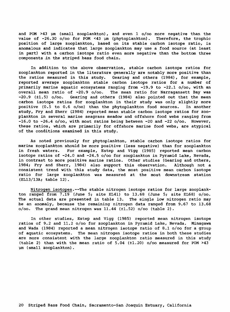
and POM >43 ym (small zooplankton) , and even 1 o/oo more negative than the value of -26.30 o/oo for POM <43 ym (phytoplankton) . Therefore, the trophic position of large zooplankton, based on its stable carbon isotope ratio, is anomalous and indicates that large zooplankton may use a food source (at least in part) with a carbon isotope ratio even more negative than the bottom three components J.n the striped bass food chain.

In addition to the above observation, stable carbon isotope ratios for zooplankton reported in the literature generally are notably more positive than the ratios measured in this study. Gearing and others (1984), for example, reported average zooplankton stable carbon isotope ratios for a number of primarily marine aquatic ecosystems ranging from -19.9 to -22.1 o/oo, with an overall mean ratio of -20.9 o/oo. The mean ratio for Narragansett Bay was-20.9 (±1.5) o/oo. Gearing and others (1984) also pointed out that the mean carbon isotope ratios for zooplankton in their study was only slightly more positive (0.5 to 0.6 o/oo) than the phytoplankton food sources. In another study, Fry and Sherr (.1984) reported mean stable carbon isotope ratios for zooplankton in several marine seagrass meadow and offshore food webs ranging from-16.0 to -26.4 o/oo, with most ratios being between -20 and -22 o/oo. However, these ratios, which are primarily for offshore marine food webs, are atypical of the conditions examined in this study.

As noted previously for phytoplankton, stable carbon isotope ratios for marine zooplankton should be more positive (less negative) than for zooplankton in fresh waters. For example, Estep and Vigg (1985) reported mean carbon isotope ratios of -24.0 and -24.5 o/oo for zooplankton in Pyramid Lake, Nevada, in contrast to more positive marine ratios. Other studies (Gearing and others, 1984; Fry and Sherr, 1984) also support this observation. Although not a consistent trend with this study data, the most positive mean carbon isotope ratio for large zooplankton was measured at the most downstream station (EL13/13A; table 12).

Nitrogen isotopes. The stable nitrogen isotope ratios for large zooplank ton ranged from 7.19 (June 5; site EL41) to 13.68 (June 5; site EL68) o/oo. The actual data are presented in table 13. The single low nitrogen ratio may be an anomaly, because the remaining nitrogen data ranged from 9.67 to 13.68 o/oo. The grand mean nitrogen was 11.44 (±1.52) o/oo (table 2).

In other studies, Estep and Vigg (1985) reported mean nitrogen isotope ratios of 9.2 and 11.2 o/oo for zooplankton in Pyramid Lake, Nevada. Minagawa and Wada (1984) reported a mean nitrogen isotope ratio of 8.1 o/oo for a group of aquatic ecosystems. The mean nitrogen isotope ratios in both these studies are more consistent with the large zooplankton ratio measured in this study (table 2) than with the mean ratio of 5.04 (±1.20) o/oo measured for POM >43 ym (small zooplankton).


Neomysis Shrimp

Carbon isotopes. The mean stable carbon isotope ratios for Neomysis shrimp ranged from -21.91 (May 7; site EL13/13A) to -27.11 (April 25; site EL68) o/oo, although most of the data were between -24 to -27 o/oo. The actual data are presented in table 14. The grand mean carbon isotope ratio for Neomysis shrimp was -25.89 (±1.37) o/oo (table 2).

The mean carbon ratios for the four sampling sites ranged from -24.43 (±1.60) o/oo at the more marine-like downstream site (EL13/13A) to a more nega tive ratio of -26.69 (±0.22) o/oo at the upstream site (EL51). The grand mean carbon ratio for Neomysis shrimp was about 1 o/oo less negative than the mean ratios for detritus, POM <43 ym (phytoplankton) , POM >43 ym (small zooplankton), and large zooplankton (table 2). Assuming that the stable carbon isotope ratio becomes more positive as one goes from the lower to higher trophic levels in a food chain, Neomysis shrimp theoretically could use one or more of these lower trophic components as food sources.

Nitrogen isotopes. The mean stable nitrogen isotope ratios for Neomysis shrimp ranged from 10.18 (August 13; site EL51) to 12.89 (August 13; site EL68) o/oo. The actual data are presented in table 15. The grand mean nitrogen ratio was 11.24 (±0.80) o/oo (table 2).

The mean nitrogen isotope ratio for Neomysis shrimp was similar to the ratio of 11.44 (±1.52) o/oo measured for large zooplankton (table 2), indica ting that both groups occupy a similar position in the trophic structure of the striped bass food chain, and that Neomysis shrimp do not utilize large zooplankton as a primary nitrogen source. Furthermore, the nitrogen isotope ratio for Neomysis shrimp and large zooplankton is about 6 o/oo more positive than that for detritus, POM <43 ym (phytoplankton), and POM >43 ym (small zooplank ton) . Ideally, one expects an increase of about 3 o/oo between adjacent trophic levels in a food chain. Therefore, the 6 o/oo difference between Neomysis shrimp and large zooplankton, and the bottom three components of the striped bass food chain (table 2) indicates the -possibility that two trophic levels, rather than one, may exist between the trophic level occupied by the bottom three components. It also indicates that these two consumers may not utilize the bottom three components either directly or exclusively as primary food sources.


Larval Striped Bass

Carbon isotopes. As noted previously, because of gaps in the data, the striped bass data were grouped on the basis of specific lengths of fish to obtain mean isotope values. The actual data are presented in table 16. The individual stable carbon isotope ratios for the less than 6-mm length striped bass ranged from -21.18 (April 25; site EL51) to -25.36 (June 18; site EL41) o/oo, and those for the 6- to 12-mm length fish ranged from -19.17 (June 18; site EL68) to -25.38 (July 12; site EL13/13A) o/oo (table 16). The range in the mean ratios of the smaller fish was larger than that of the longer fish. The individual carbon isotope ratios for the 13- to 20-mm fish ranged from-23.75 (June 18; site EL68) to -27.01 (July 2; site EL13/13A) , the 21- to 30-mm fish ranged from -23.27 (July 26; site EL68) to -25.33 (June 27; site EL68) o/oo, and the 31- to 40-mm fish ranged from -23.32 (July 2; site EL68) to-25.96 (June 27; site EL68) o/oo. The greater than 40-mm fish were represented by a single carbon isotope ratio of -24.60 o/oo (July 26; site EL68).

The mean stable carbon isotope ratios for striped bass of 12 mm or less length were more positive than -24 o/oo (table 16) . In contrast, the mean ratios for the four groups of fish greater than 12 mm length were more negative than -24 o/oo. Although the standard deviations do overlap (table 3) , the small break in the mean carbon isotope ratios at the 12 mm length may indicate a transition from a predominantly endogenous food source (the yolk sac) to a predominantly exogenous food source (Neomysis shrimp and (or) other similar- sized organisms). This is consistent with observed feeding patterns for larval striped bass (Lee Miller, California Department of Fish and Game, oral commun., 1984). Between these two stages, larval striped bass seem to feed on copepod larvae and cladocerans (Miller, 1987). Analysis of a greater number of striped bass ranging between about 5 to 15 mm in length is necessary to more clearly illustrate the dynamics of this transition phase.

Other studies on the stable carbon isotope characteristics of fish gener ally do not provide information specific to striped bass. Fry and Sherr (1984) reported mean carbon isotope ratios ranging from -15.9 (±1.4) to -19.0 (±1.3) o/oo in a number of marine offshore food webs. Wiersema and others (1982) reported mean carbon isotope ratios for animals (primarily fish) in Matagorda Bay, Texas, ranging from -30.8 o/oo in the upstream freshwater inflow end of the bay to -14.2 o/oo in the marine end of the bay system. There was a gradi ent to less negative mean carbon ratios as one moved from the upstream to the downstream end of the bay. Estep and Vigg (1985) reported mean carbon ratios ranging from -22.7 to -23.1 o/oo in Pyramid Lake, Nevada. A larger range was seen in fish from Lahontan Reservoir, Nevada, with mean ratios ranging from-16.8 o/oo for Tahoe sucker to -25.9 o/oo for small crappie and catfish. Most mean ratios for fish in Lahontan Reservoir were between -20 and -23 o/oo. These data indicate that mean carbon isotope ratios for fish depend on such factors as the specific fish species, the characteristics of the aquatic environment, and the specific food sources.


TABLE 3. Mean stable carbon and nitrogen isotope ratios for two groupings of striped bass

[N, number of samples used to calculate grand mean ratio. Grand means were calculated using all data for a component, regardless of sampling date or site, mm, millimeters; o/oo f per mil]

Grand mean stable isotope ratios (o/oo)jjengtn ui

striped bass (mm)

12 or less

Greater than 12

N

11

14

Carbon

-23.36

-24.60

Standard deviation

±2.22

±1.10

N

11

14

Nitrogen

16.00

13.32

Standard deviation

±3.66

±0.49

Nitrogen isotopes. The data for stable nitrogen isotopes were grouped in the same manner as the carbon isotopes. The nitrogen ratios for striped bass less than 6 mm ranged from 14.56 (June 18; site EL41) to 25.17 (April 25; site EL51) o/oo. The actual data are presented in table 17. The mean nitrogen iso tope ratios for the 6- to 12-mm striped bass ranged from 12.22 (June 18; site EL68) to 19.38 (June 18; site EL13/13A) o/oo. In both cases, the large range in isotope values was due to a single high value, which may represent anomalies, because the remaining data were much more closely grouped.

The mean nitrogen isotope ratios for the 13- to 20-mm fish ranged from 12.43 (June 18; site EL68) to 13.75 (July 2; site EL13/13A) o/oo, the 21- to 30-mm length fish ranged from 12.61 (June 27; site EL68) to 13.91 (July 26; site EL68) o/oo, and the 31- to 40-mm fish ranged from 13.00 (June 18; site EL68) to 13.91 (July 26; site EL68) o/oo (table 17). The single value for the greater than 40-mm fish was 13.30 o/oo.

As with the mean carbon ratios, the mean stable nitrogen isotope ratios also indicate a shift in primary food sources as the striped bass increase in length. Although the standard deviations overlap, the mean nitrogen ratio for all striped bass 12 mm in length or less (table 3) was 16.00 (±3.66) o/oo and the mean ratio for striped bass longer than 12 mm was 13.32 (±0.49) o/oo. Thus, the two smallest length fish groups have a mean stable nitrogen isotope ratio nearly 3 o/oo more positive than the mean ratio of the four larger sized fish about one trophic level.

All mean nitrogen isotope ratios for the striped bass 12 mm or longer in length are greater than 13.20 o/oo (table 2) , which is about 2 o/oo more positive than the mean value of 11.24 (+0.80) o/oo for Neomysis shrimp. These data support the generally held view that longer striped bass feed primarily on Neomysis shrimp. The mean nitrogen isotope ratio for large zooplankton (table 2) indicates these organisms also can be a food source for striped bass. However, on the basis of the nitrogen isotope data, neither Neomysis shrimp nor large zooplankton seemed to be a major food source for striped bass less than 12 mm in length.


Other studies do not provide information on stable nitrogen isotope ratios specific for striped bass. Minagawa and Wada (1984) reported a mean nitrogen ratio of 11.1 o/oo for fish taken from Lake Ashinoko, Japan. The range in measured ratios was small, from 10.7 to 11.6 o/oo. Estep and Vigg (1985) reported mean nitrogen ratios ranging between 9.9 and 11.6 o/oo for tui chubs (Gila bicolor) in Pyramid Lake, Nevada, similar to that reported for Lake Ashinoko. They also reported that mean nitrogen isotope ratios for Lahontan Reservoir, Nevada, ranged from a low value of 9.5 o/oo for Sacramento blackfish to 16.2 o/oo for catfish, with most ratios being between 10 and 13 o/oo.

Municipal Waste water-Treatment Plant Effluents

Carbon isotopes. The stable carbon isotope ratios for the Sacramento and Stockton municipal wastewater-treatment plant effluents were extremely uniform. The actual data are presented in table 18. The grand mean stable carbon isotope ratio for the effluent samples was -24.15 (±0.04) o/oo (table 4). This ratio is more positive than the grand mean ratios of all study components other than several lengths of striped bass. It is about 2 to 3 o/oo more positive than those of the bottom three components of the striped bass food chain, which contrasts to the expected pattern if the effluents were being utilized as a primary food source by these components. Although some of the standard devia tions do overlap, the mean data are consistent with the belief that the wastewater effluents did not constitute a primary source of organic carbon for any study component, at least during the period of this study.

Nitrogen isotopes. In contrast to the carbon isotope data, the stable nitrogen isotope ratios from the two plants are distinctively different. The two stable nitrogen isotope ratios of the Sacramento plant effluent were 1.60 and 2.01 o/oo, for a mean nitrogen ratio of 1.80 (±0.29) o/oo (table 19). These values are similar to the ratio of 1.0 o/oo reported for the Reno-Sparks (Nevada) sewage treatment plant (Estep and Vigg, 1985). However, the stable nitrogen isotope ratios of the Stockton plant effluent were 15.51 and 15.07 o/oo, for a mean nitrogen ratio of 15.29 (±0.31) o/oo. Based on these ratios, the mean stable nitrogen isotope ratio for the plant effluents (table 4) was 8.55 o/oo, with a large standard deviation of ±9.54 o/oo.

These differences in the mean stable nitrogen isotope ratios may reflect the different wastewater-treatment processes used at the two plants. The Sacramento plant is an activated sludge, secondary-treatment plant. The Stockton plant is a secondary treatment, sewage lagoon plant throughout most of the year. However, during the summer months (when the samples were collected), the Stockton plant is operated as a tertiary treatment plant, using mixed-media filtration of the effluent prior to its discharge. This tertiary treatment process has the effect of removing nitrogen from the lagoon waters by the fil tration of algal cells from the lagoon effluent, in contrast to the secondary treatment used at the plant throughout the remainder of the year. However, stable nitrogen isotope data were not available for the Stockton plant for the period when only secondary treatment of sewage was being practiced.


TABLE 4. Mean stable carbon and nitrogen isotope ratios for municipal wastewater-treatment plant effluents

[N, number of samples used to calculate mean value. Grand means were calculated using all data for a component, regardless of sampling date or site, o/oo, per mil]

Municipal Grand mean stable isotope ratios (o/oo)wastewater-

treatment Standard Standardplant N Carbon deviation N Nitrogen deviation

Sacramento 2 -24.12 ±0.05 2 1.80 ±0.29

Stockton 2 -24.18 ±0.12 2 15.29 ±0.31

Grand mean 4 -24.15 ±0.04 4 8.55 ±9.54

An additional factor to consider is the nature of the wastes treated at the two plants. Both plants receive primarily municipal and industrial wastes throughout the year. In addition, the Stockton plant also receives large loads of vegetable matter from food-processing plants on a seasonal basis. Neverthe less, the mean nitrogen isotope ratios for the two effluents are sufficiently different from the mean nitrogen ratios of the food chain components examined in this study that the effluents do not seem to be a significant nitrogen source for them, at least not directly. The exception is that the data for the Stockton plant (tables 18 and 19) are consistent with the possibility that it could serve as an organic carbon and nitrogen source for the striped bass less than 6 mm in length (table 2) . However, as previously indicated, this length class of striped bass subsist primarily on the remnants of their yolk sac. Therefore, they are less likely to rely on exogenous sources of nitrogen or carbon than any other group of striped bass. In addition, the distance of the Stockton plant from the striped bass spawning area (fig. 1) is sufficiently great that the plant effluent is not likely transported to the spawning area.

CARBON AND NITROGEN FLUX BETWEEN TROPHIC LEVELS

The primary purpose of this section is to examine the changes in the mean isotope ratios from the lower trophic levels to the higher trophic levels of the striped bass food chain. Other investigators (Rau and others, 1983; Fry and Sherr, 1984; Gearing and others, 1984) have suggested that, under ideal conditions, one would expect to see an increase of about 1 o/oo in the stable carbon isotope ratio as one progressed from prey organisms on one trophic level to predator organisms on the next higher trophic level. The corresponding

Carbon and Nitrogen Flux 25

increase in the stable nitrogen isotope ratio between adjacent trophic levels is about 3 o/oo. A specific population of organisms using a single, primary food source would represent ideal conditions for this energy transfer between trophic levels. In this study, this positive increase in the mean isotope ratio should occur at each transfer of energy (carbon and nitrogen) in the hypothesized phytoplankton/detritus >zooplankton/#eomysis shrimp >striped bass food chain.

25

20

CO

15

10

5 -

Stockton municipal wastewater- treatment plant

i Striped bass (31-40 mm)

Large zooplankton

Slope of line of best fit= 1.91:1

based on all data

Striped bass (6-12 mm)

-Striped bass .(21-30 mm)

^Striped bass(>40 mm)

Neomysis shrimp

POM>43 Jim (small

zooplankton)

> H-H* POM

<43ym (phytoplankton)

mm Length of striped bass, in millimeters

Range bars - ± one standard deviation around mean value

I I

"Sacramento municipal wastewater- treatment plant

I I I I I-30 -25 -20

STABLE CARBON ISOTOPE RATIO (PER MIL)

-15

FIGURE 2.-Grand mean stable carbon and nitrogen isotope ratios and standard deviations for study components. (Data taken from table 2.)


The grand mean carbon and nitrogen isotope ratios for the components of the striped bass food chain were plotted on an arithmetic scale (fig. 2) . If the ideal 1 o/oo and 3 o/oo positive increase in the carbon and nitrogen isotope ratio is maintained in the striped bass food chain, one would expect to see a straight line with a slope of 3:1. In fact, the data measured in this study do result in a general increase to more positive (less negative) values as one goes up the striped bass food chain (fig. 2).

Based on the mean stable isotope ratios, the slope of the line-of-best-fit illustrated in figure 2 is 1.91:1, with a correlation coefficient of 0.55 (table 5). However, several lines-of-best-fit are possible, based primarily on the specific groupings of striped bass and municipal wastewater-treatment plants used in their calculation. For example, the Sacramento municipal wastewater-treatment plant is a considerable distance upstream in the Sacra mento River from the study site (fig. 1) and occupies an anomalous position in

TABLE 5. Alternative lines-of-best-fit for striped bass food chain components

[Grand mean values of all components were taken from table 2. Numbers refer to mean values of food chain components in table 2, which were considered in developing alternative lines-of-best-fit for figure 2, as follows:

1, detritus;2, POM <43-ym (phytoplankton) ;3, POM >43-ym (small zooplankton) ;4, large zooplankton;5, Neomysis shrimp;6, striped bass <6 mm;7, striped bass 6 to 12 mm;8, striped bass 13 to 20 mm;9, striped bass 21 to 30 mm;

Components Correlationconsidered coefficient

1-13 0.55

1-5, 12-15 .43

1-12 .84

1-5, 12, 14-15 .81

1-11 .83

1-5, 14-15 .77

10, striped bass 30 to 40 mm;11, striped bass >40 mm;12, Stockton municipal wastewater-

treatment plant;13, Sacramento municipal wastewater^

treatment plant;14, striped bass <6 to 12 mm;15, striped bass >12 mm.ym, micrometers; mm, millimeters]

Slope(N:C) Intercept

1.91:1 59.0

1.46:1 46.8

2.45:1 73.6

2.44:1 73.3

2.40:1 72.1

2.30:1 69.3


figure 2. If this data point is omitted from the calculation, the resultant line-of-best-fit is markedly improved, with a slope of 2.45:1 and a correlation coefficient of 0.84. This latter combination of food chain components (table 5) produced the line-of-best-fit with the best statistical characteristics for the available data. Removal of the data for both plants from the calculations (table 5) results only in a very small decrease in the slope of the line-of- best-fit (2.40:1) and the correlation coefficient (0.83). This is due to the likely fortuitous position of the mean data point for the Stockton plant among the mean data points for the various groupings of striped bass. Therefore, for the reasons mentioned previously, the municipal wastewater-treatment plant effluents likely do not have a direct role in the striped bass food chain.

Several inconsistencies also are observed with the relations presented in figure 2. The mean carbon and nitrogen isotope ratios for the POM <43 ym (phytoplankton), POM >43 ym (small zooplankton), and detritus samples do not plot as distinct components. Rather, the grand mean ratios of these components (thought to comprise the base of the striped bass food chain in this study) are very similar (table 2) . The ratios for the POM >43 ym (small zooplankton) and the detritus samples virtually overlap, indicating that they may be composed of the same (or very similar) components. This is further demonstrated with a more detailed representation of these components (fig. 3) . The mean carbon isotope ratio for POM <43 ym (phytoplankton) was more positive than the ratio for either POM >43 ym (small zooplankton) or detritus. The mean nitrogen isotope ratios were similar for all three components.

One possible explanation for these similar stable isotope ratios may involve the sampling methodology. Because of the field procedures used to collect the samples, possible isolation of common materials in all three components can result in an overlap of the mean isotope ratios for these components. The separation methods used in this study did not allow for a finer separation of these three lower trophic level components. Although the data do not clearly illustrate the presumed phytoplankton/detritus >zooplankton pathway, the results are consistent with the generally held belief that these three components do compose the lower trophic end of the striped bass food chain.

The next higher trophic components in the striped bass food chain, large zooplankton and Neomysis shrimp, had a more positive mean nitrogen isotope ratio than the three lower trophic level components. The mean carbon ratio for Neomysis shrimp is about 1 o/oo more positive than the three lower trophic components, which is consistent with the possibility that Neomysis shrimp could use phytoplankton, small zooplankton, and (or) detritus as a food source.


cr 7LU Q.

LU Q. O

S 6C/3

LUO O crHZ LU _l CO

^

(Small zooplankton) Grand mean

1

STATION

O EL13/13A

V EL68 D EL41 O EL51

Range bars - ;

COMPONENT DESIGNATION (using station EL13/13A as example)

Detritus

d POM < 43 um (phytoplankton)

© POM >43 um (small zooplankton)

: one standard deviation around mean value

Detritus,-Grand mean

-O

M

POM<43um(phytoplankton)

Grand mean

-28 -27 -26

STABLE CARBON ISOTOPE RATIO (PER MIL)

-25

FIGURE 3.-Mean stable carbon and nitrogen isotope ratios and standard deviations for detritus, POM <43 ym (phytoplankton) and POM >43 um (small zooplankton). (Site mean values and standard deviations taken from tables 6-11. Grand mean values taken from table 2.)


In addition, the mean nitrogen ratio for Neomysis shrimp is nearly 6 o/oo more positive than these lower trophic level components (table 2) . However, assuming that one or more of these components are a primary food source for Neomysis shrimp (that is, Neomysis shrimp occupies the next highest trophic level in the food chain) , one normally would expect only a 3 o/oo increase in the nitrogen isotope ratio for Neomysis shrimp. The measured 6 o/oo increase in the mean stable nitrogen isotope ratio indicates that an additional trophic level may exist between that represented by the three lowest trophic level components in the striped bass food chain and that represented by large zooplankton and Neomysis shrimp. The data also indicate that this potential additional trophic level was not sampled in this study. On the basis of the expected pattern of stable isotope enrichment, this unidentified component should have a stable carbon isotope ratio of about -28 o/oo and a stable nitrogen isotope ratio of about 8 o/oo. These isotope ratios span the values between the three lowest trophic level components and the trophic level repre sented by large zooplankton and Neomysis shrimp.

The mean stable carbon isotope ratio for large zooplankton is the most negative and most anomalous of all the components examined in this study. This is because one would normally expect a more positive stable isotope ratio for large zooplankton than for its presumed food sources, which is contrary to the results obtained in this study. The grand mean carbon isotope ratio obtained in this study (fig. 2; table 2) is consistent with the possibility that large zooplankton could use a mixture of one or more of the three lower trophic level components, plus an unidentified component with a distinctly more negative carbon isotope ratio than any other component examined in this study. As previously noted, Simenstad and Wissmar (1985) reported a mean carbon isotope ratio of -28.9 o/oo for deciduous and coniferous debris in their study in a side channel of a long fjord (Hood Canal) off Puget Sound, Washington. The Sacramento-San Joaquin Estuary also contains appreciable quantities of various types of organic debris from the surrounding terrestrial and aquatic environ ment. For example, peat is found in appreciable quantities in this estuarine system. On the basis of studies done on estuarine food webs in the Alaskan Beaufort Sea, Schell (1983) reported average stable carbon isotope ratios for peat ranging between about -27 to -30 o/oo, which are more negative than any component of this study. However, the characteristics of the Alaskan Beaufort Sea Estuary are markedly different from those of this estuarine system. Thus, the applicability of these Arctic carbon isotope data for peat to the Sacramento-San Joaquin Estuary is unknown. Samples of peat from the Sacramento-San Joaquin Estuary were not collected during this study.

The mean stable nitrogen isotope ratio for large zooplankton indicates they occupy the same trophic level as Neomysis shrimp, in spite of the differ ences in their mean carbon isotope ratios (fig. 2). Both organisms have mean nitrogen isotope ratios about 6 o/oo more positive than the three components at the bottom of the food chain. Thus, a similar trophic level is possible if large zooplankton and Neomysis shrimp utilize the previously indicated, uniden tified component as a primary nitrogen source. This unidentified component would occupy a trophic level between the bottom three food chain - components and the large zooplankton/JVeomysis shrimp trophic level. However, although the standard deviations do overlap, the more negative stable carbon isotope ratio for large zooplankton, compared to Neomysis shrimp, indicates another


(or additional) primary carbon source for large zooplankton. It was not possible, however, to explore this possibility further with the data available in this study.

The striped bass data (fig. 2) indicated distinct food habits at different growth stages. The two smaller lengths of striped bass had the most positive mean carbon and nitrogen isotope ratios. Although the standard deviations overlapped, the mean nitrogen ratios for these two smallest lengths of fish were separated by about 3 o/oo, indicating the possibility of different primary food sources. This is consistent with the previous suggestion that striped bass less than 6 mm in length subsist on the yolk sac remnants, and those 6 to 12 mm in length are beginning to use zooplankton and (or) Neomysis shrimp as primary food sources.

In contrast to the smaller fish, the carbon and nitrogen isotope ratios for the four longer length striped bass are similar. These similar ratios and their more positive positions relative to Neomysis shrimp and large zooplankton support the possibility that striped bass change to these latter food sources by the time they have reached a length of 12 mm. In addition, the primary food sources for striped bass seemed to remain unchanged beyond this point, at least up to a length greater than 40 mm.

The data for the wastewater-treatment plant effluents do not support a direct role for these carbon and nitrogen sources in the striped bass food chain. It is noted that fish often are present in large numbers in areas where municipal wastewater-treatment plant effluents are discharged. This phenomenon may represent an opportunity for the fish to feed on zooplankton and other organisms whose production might have been stimulated by increased bacterial productivity resulting from bacterial use of dissolved carbon (rather than particulate organic carbon) in the effluents (Rau and others, 1981). This would constitute an indirect use of the effluent nutrients through consumption of intermediate trophic-level consumers by striped bass, in contrast to a direct use of the effluents by the fish. This possibility is consistent with the mean carbon and nitrogen isotope ratios for zooplankton, Neomysis shrimp, and striped bass measured in this study. However, the position of the data point for the Sacramento plant (fig. 2) indicates it is not a primary food source for the striped bass food chain. The position of the data point for the Stockton plant (fig. 2) is consistent with the possibility that it might serve as a nitrogen and carbon source for the smallest (less than 6 mm) striped bass. However, as previously indicated, the smallest striped bass generally subsist on the remnants of their yolk sac, rather than on exogenous food sources.

On the basis of these results, figure 2 supports the general food chain for striped bass in the Sacramento-San Joaquin Estuary as described by fisher ies scientists studying the estuary. The measured carbon and nitrogen trans fers up the various trophic levels in the presumed striped bass food chain are reasonable and consistent with presumed food chain relations in the estuary. An inability to isolate homogeneous samples of the lower three trophic level components of the food chain did not allow for a more detailed assessment of carbon and nitrogen transfers between the lower and middle trophic levels of the food chain.


The possibility of unsampled component(s) in a trophic level between the trophic level represented by the lower three components of the food chain and that represented by large zooplankton and Neomysis shrimp warrants further study. The carbon isotope characteristics of the large zooplankton, relative to the lower trophic level organisms which they might use as food sources, is inconsistent with the expected positive increase in the carbon ratio as one progresses from lower to higher trophic levels. The carbon data indicate that large zooplankton also may use one or more of these three components, plus an unidentified component with more negative carbon isotope ratios than those measured in this study, as food sources. Some possibilities, which cannot be substantiated with the available data, are peat, carbon-13 depleted phytoplankton, and perhaps dissolved organic carbon.

These conclusions are consistent with the findings of a 1986 study of the food habits of larval striped bass in the Sacramento-San Joaquin Estuary. On the basis of an analysis of the stomach content of about 10,000 larval striped bass, cyclopoid and calanoid copepodids, Eurytemora, Sinocalanus, and Bosmina were reported to be the main food organisms (in terms of numbers) in the stomachs of 5- to 14-mm length striped bass larvae taken from the lower Sacramento River (Miller, 1987). The abundance of Bosmina and cyclopoid and calanoid copepodids decreased as the size of the larvae increased. Neomysis shrimp was not consumed by striped bass larvae less than 7 mm in length, and increased in abundance thereafter with increasing size of the larvae. The most abundant organisms in striped bass larvae from the lower San Joaquin River were Bosmina and Eurytemora. The abundance of Eurytemora increased and Bosmina decreased with increasing size of the striped bass larvae. In terms of biomass, Cyclopidae, Eurytemora, Sinocalanus, Diaptomus, Acartia, and Daphnia each constituted about 10 to 12 percent of the total dry weight biomass in the stomachs of the striped bass larvae (Miller, 1987). Thus, although cyclopoid and calanoid copepodids were present in greater numbers in the stomachs of striped bass larvae, the larger size of the other zooplankton identified above contributed to their greater significance in terms of total dry weight biomass.

TEMPORAL AND SPATIAL VARIATIONS

The mean stable isotope ratios also were examined as a function of the sampling sites (figs. 4 and 5) , the sampling dates (figs. 6 and 7) , and the individual components (figs. 8 to 17) . Because of their inconsistent spatial and temporal coverage, neither the striped bass nor the municipal wastewater- treatment plant data are included in these diagrams. Instead, the focus is on the lower- and middle-level components of the striped bass food chain. In addition, some isotope ratios represented only one data point. Therefore, the data are used here primarily as an overview of general characteristics, rather than as detailed descriptions of specific temporal or spatial patterns.


Mean Isotope Ratios by Sampling Site

With the exception of Neomysis shrimp at sampling site EL13/13A, the mean carbon isotope ratios for all five components examined ranged between -26 and -28 o/oo at the four sites. The carbon data (fig. 4) generally illustrate a shift to more negative ratios as one progresses from the marine-like downstream site (EL13/13A) to freshwater-like upstream sites (EL41 and EL51). This is consistent with previous studies in other estuarine systems (Fry and Sherr, 1984) . Sampling site EL68 is near the downstream end of the striped bass nursery area. However, this site actually is about 0.5 mile down a slough adjacent to the Sacramento-San Joaquin River channel (fig. 1) , rather than in the main river channel area. As shown in subsequent figures, the stable isotope ratios at this site commonly exhibited an inconsistent pattern, rather than characteristics intermediate between the more marine-like downstream site EL13/13A and the more freshwater-like upstream sites EL41 and EL51.

In contrast to the carbon data, the mean nitrogen isotope ratios (fig. 5) are segregated into two distinct groups. Most of the mean nitrogen isotope ratios for large zooplankton and Neomysis shrimp were between 10 and 12 o/oo

£.V

CCLU Q.

O1-

cc -24LU 0. O1-

oCO

0 -26CO CC

ozLU2 -28

-30

1 1 1 1 1

O

A o o -A A A A

-f Q o n n n

i I 1 i lEL13/13A EL68 EL41 EL51 GRAND

MEAN SAMPLING SITE

EXPLANATION

-f DETRITUS

A POM <43 um (PHYTOPLANKTON)

O POM >43 um (SMALL ZOOPLANKTON)

D LARGE ZOOPLANKTON

O NEOMYSIS SHRIMP

FIGURE 4.-Mean stable carbon isotope ratios, by site.

Temporal and Spatial Variations 33

LJJCD O IT

14

12

A

O

J_

0

EL13/13A EL51 GRAND MEAN

EL68 EL41

SAMPLING SITE

FIGURE 5.-Mean stable nitrogen isotope ratios, by site.

EXPLANATION

+ DETRITUS

A POM <43 Um(PHYTOPLANKTON)

O POM >43 um (SMALL ZOOPLANKTON)

D LARGE ZOOPLANKTON

O NEOMYSIS SHRIMP

for all four sampling sites. In contrast, the mean ratios for the three lower trophic level components generally were between 4 and 7 o/oo. Although the mean nitrogen isotope ratio for POM <43 ym (phytoplankton) was nearly constant for all four sites, there was an increase of about 1 o/oo for POM >43 ym (small zooplankton) , and a decrease of about 1 o/oo for detritus, between the two upstream and downstream sites. Overall the mean stable isotope ratios do not show marked spatial changes across the sampling area during the study period.

Mean Isotope Ratios by Sampling Date

With the exception of Neomysis shrimp, the stable carbon isotope ratios (fig. 6) generally were between -26 and -28 o/oo. The mean carbon ratios for Neomysis shrimp tended to be 1 to 2 o/oo more positive than the other components on most sampling dates.

The stable nitrogen isotope data (fig. 7) also showed the bimodal group ings previously noted in figure 5. The two higher trophic level components were about 6 o/oo more positive than the other three lower trophic level com ponents. Overall, temporal changes are not markedly different in either the carbon or nitrogen ratios during the study period.


"u 1 1 1 1

^-22- ^ ^ccLUQ_

01-

LT -24 LLJQ.O

£ 0CO

0 -26 - O ACO A Aoc A O

O 6 A, 8z $ 0 +< nLU U2 -28 -

3CO

oc

30 1 1 125 7 21 5 18

APR MAY JUNE

I I I

_

^0 0o o

AA A

° &I i^ j i

n «X3QC

1 1 1 1 1

EXPLANATION

-1- DETRITUS

A POM <43 Mm(PHYTOPLANKTON)

O POM >43 ym (SMALLZOOPLANKTON)

D LARGE ZOOPLANKTON

O NEOMYSIS SHRIMP2 12 30 13 GRAND

JULY AUG MEAN

SAMPLING DATE

FIGURE 6. -Mean stable

14 , , , , ,

3 12 -

tr vLU <S

i n So 10-

trLUQ_OO 8 ~~CO

zLUCj _u -L.**J l^ ^59 fttr 6 A n| _ *-» V_J

2 ° ° A +LU +0

^ 4 _ « ACO o0c

2 1 1 1 1 L__25 7 21 5 18

APR MAY ,JUNE _

carbon isotope ratios, by date.

ill I

n o

X^ /S, >r

d 4"

i §CO

QC

I I I

EXPLANATION

+ DETRITUS

A POM <43 Mm (PHYTOPLANKTON)

0 POM >43 um (SMALLZOOPLANKTON)

D LARGE ZOOPLANKTON

O NEOMYSIS SHRIMP2 12 30 13 GRAND

JULY AUG MEAN

SAMPLING DATE

FIGURE 7.-Mean stable nitrogen isotope ratios, by date.


Mean Isotope Ratios for Specific Study Components

Detritus

The mean carbon isotope ratios for detritus (fig. 8) were between -26 and -28 o/oo, similar to those of POM <43 ym (phytoplankton; fig. 10) and POM >43 ym (small zooplankton; fig. 12) . The mean carbon ratios showed little variation over time.

The mean nitrogen isotope ratios (fig. 9) showed a larger variability than the carbon ratios, being similar in range to the data for POM <43 ym (phytoplankton; fig. 11) and POM >43 ym (small zooplankton; fig. 13). Temporal patterns in the isotope data were not readily discernible.

<iU

1-22

ECUJ CL

Oh-

CC -24LLI CL

O CO

0 -26CO DC

O

S -28

-30

1 1 1 1 1 1 1 1 1 1

_

D +

. D ffl ffl &8 o S A

A A (0 ^co w 75 09T3 T3 T3 T3 §OOO

C C C

1 1 I 1 I I 1 i ! I25 7 21 5 18 2 12 30 13 GRAND

EXPLANATION

+ EL13/13A

A EL68

O EL41

D EL51

APR MAY JUNE JULY AUG MEAN

SAMPLING DATE

FIGURE 8.-Mean stable carbon isotope ratios for detritus.


If

j 12

ccUJa.

Q 10

a:UJ CLOI- o0 8CO

TROGEN

O5

ZzUl

5 4

2

I I I I I I I I I I

_

+

~~ O ~~

A A A 4--a

D ° aft + " a o

CO (D CO CO"O "O -O "D

i o i i ii i i i i i i i i i

25 7 21 5 18 2 12 30 13 GRAND

EXPLANATION

+ EL13/13A

A EL68

O EL41

D EL51


SAMPLING DATE

FIGURE 9.-Mean stable nitrogen isotope ratios for detritus.


The mean carbon isotope ratios (fig. 10) generally were between -25 and -27 o/oo for all sites. The mean carbon isotope ratios for sites EL13/13A, EL41, and EL51 showed similar temporal patterns.

The nitrogen ratios (fig. 11) tended to be slightly higher at all sites for the first two sampling dates than for the remainder of the sampling period. This shift may be related to a phytoplankton bloom or die-off during one of these distinct periods.


t\)

1-22

ccLU D.

0

CE -24LU 0.o0CO

0 -26 m a:

ozLU2 -28

-30

14

d 12

a:LU D_

g 10

a:LUa. 0

rROGEN ISOT0> 00

i z zLU

5 4

2

1 1 1 1 1 1 i 1 | 1

_ _

0-(- A A ,

AD Q

sA °

_ _3 S &

1 22

1 I i l 1 I i i l i25 7 21 5 18 2 12 30 13 GRAND


SAMPLING DATE

EXPLANATION

-I- EL13/13A

A EL68

O EL41

D EL51

FIGURE 10. -Mean stable carbon isotope ratios for POM <43 pm (phytoplankton).

I I l l I i l i I I

n

_ § 0 * _

A g + O $

---- co r fj (g (g _CO ' 1 CO CO D -D -O

i g i

i 1 l 1 I i i 1 i i25 7 21 5 18 2 12 30 13 GRAND

EXPLANATION

-I- EL13/13A

A EL68

O EL41

D EL51


SAMPLING DATE

FIGURE 11.-Mean stable nitrogen isotope ratios for POM <43 urn (phytoplankton).


Participate Organic Matter >43 ym (Small Zooplankton)

The mean carbon isotope ratios (fig. 12) generally were between -26.5 and -27.5 o/oo, e slightly smaller range than observed for detritus (fig. 8) and POM <43 ym (phytoplankton; fig. 10) , with no readily apparent trends. The temporal patterns for all the stations were similar. The mean nitrogen data (fig. 13) generally showed the same range as detritus (fig. 9) and POM <43 ym (phytoplankton; fig. 11).

i -22a:LUa.

g

<r -24LU 0.0

oCO

1 CARBON 1 w0)

^LU^ -28

-30

III 1 1 1 | 1 1

_ _

_

+ + A A + 4- Q i m § A Ao A * §

a B e

«9 S «2

I 11

111 II 125 7 21 5 18 2 12 30 13 GRAND

EXPLANATION

+ EL13/13A

A EL68

O EL41

D EL51


SAMPLING DATE

FIGURE 12.-Mean stable carbon isotope ratios for POM >43 urn (small zooplankton).


1*

3 122DCLU0.

g 10DCLUQ.o£ 8CO

zLUOO

ZZ

LU

5 4

9

I I I I I I I I I I

~~ n ~~o

o0

- n Q n a -

D t o ,A

~4~ H i A A 3 A A W{oAA_

w ^ to ToTJ + TJ XJ

c + c c

i 1 1 1 1 1 1 1 1 1

EXPLANATION

+ EL13/13A

A EL68O EL41

D EL5125 7 21 5 18 2 12 30 13 GRAND

APR MAY t JUNE , JULY AUG MEAN

SAMPLING DATE

FIGURE 13.-Mean stable nitrogen Isotope ratios for POM >43 um (small zooplanWon).

Large Zooplankton

The mean carbon isotope ratios (fig. 14) showed a larger range than either detritus (fig. 8) , POM <43 pm (phytoplankton; fig. 10) or POM >43 ym (small zooplankton; fig. 12). Temporal patterns were not apparent, although all four sites had more negative carbon isotope ratios between the June 18 and July 2 sampling dates.

With the exception of the June 5 sampling date, the mean nitrogen isotope data (fig. 15) show higher values and a smaller range than either detritus (fig. 9), POM <43 ym (phytoplankton; fig. 11) or POM >43 ym (small zooplankton; fig. 13). Patterns were not readily discernible.

40 Striped Bass Food Chain, San-Joaquin Estuary, California

AJ

^-22

ccLU Q.

OH

ol -24LU Q. 0

0 CO

0 -26CQ CC <OzLU^ -28

-30

1 1 1 1 1 1 1 1 1 1

_

O

+ A A

o n + +no g

Q A ACO. CO LJ CO CO

CO CO CO COo "O O ^ ^

i A i i ii 1 1 1 1 1 1 1 1 1

25 7 21 5 18 2 12 30 13 GRAND

EXPLANATION

-h EL13/13A

A EL68

0 EL41

D EL51


SAMPLING DATE

FIGURE 14.-Mean stable carbon isotope ratios for large zooplankton.

It

d 12

ccLU O.

g 10

ccLU Q. OH o 0 8 COfROGEN I

a>

zz111

5 4

2

i i i A ' ' ' ' ' '

a - -g D

+ 8 + + o

A

O

to ~ 83

1 1 111 1 1 i 1 1 1 1 1 1

25 7 21 5 18 2 12 30 13 GRANDAPR MAY . _JUNE , _ JULY AUG MEAN

SAMPLING DATE

EXPLANATION

-I- EL13/13A

A EL68

O EL41

D EL51

FIGURE 15.-Mean stable nitrogen isotope ratios for large zooplankton.


Neomysis Shrimp

Mean carbon isotope data were sparse for some sampling sites and dates (fig. 16) . The two downstream sites (EL13/13A and EL68) showed the greatest variability. In contrast, the range in the mean values for the two upstream sites (EL41 and EL51) was small, generally between -26.5 and -27.5 o/oo. Temporal trends were not readily apparent in the carbon data.

Compared to the carbon data, the mean nitrogen isotope ratios for Neomysis shrimp (fig. 17) showed similar patterns and had little variability, with an overall range of about 3 o/oo. The data for the two downstream sites were about 0.5 to 1.5 o/oo more positive than for the two upstream sites. I The mean nitrogen ratio for Neomysis shrimp was about 5 to 6 o/oo more positive than detritus (fig. 9), POM <43 ym (phytoplankton; fig. 11) or POM >43 ym (small zooplankton; fig. 13), highlighting their higher level in the trophic structure of the striped bass food chain.

£M

4-22

octuCL

g<cct -24tuCLOh- OCO

0 -26CD GC

5zHI2-28

-30

1 ! 1 1 1 I 1 1 I !

+

_i_

A A ++

"*"

- A D A

QA QOn A nQ A 0 fi °

_ _«S 2 co coXJ XJ

0 0c c

1 1 1 1 1 1 I 1 1 !25 7 21 5 18 2 12 30 13 GRAND

EXPLANATION

+ EL13/13A

A EL68

0 EL41

D EL51

APR , MAY .JUNE JULY t AUG MEAN

SAMPLING DATE

FIGURE 16.-Mean stable carbon isotope ratios for Neomysis shrimp.


It

d 12

DCLJU CL

1 10DCLJU D_ 01 o

CO

TROGEN

O)

zzLJU

2 4

2

I 1 1 1 1 1 1 1 1 1

~ A * A * -^ft i

n Q 4t

o B o n

3 3 03 03 "O "O

2 i

1 1 1 1 I 1 1 1 1 125 7 21 5 18 2 12 30 13 GRAND

EXPLANATION

+ EL13/13A

A EL68

O EL41

D EL51

APR , MAY t ,JUNE , JULY _ AUG MEAN

SAMPLING DATE

FIGURE 17.-Mean stable nitrogen isotope ratios for Neomysis shrimp.

Mean Isotope Ratios at Individual Sampling Sites

The data sets for the individual sites are less consistent than the grouped data, making it more difficult to derive statistically valid trends or general relations. Consequently, the data are not presented here in graphic form.

However, examination of the mean carbon and nitrogen isotope ratios for the individual sites (tables 6-19) did show the same general characteristics and trends as previously noted for the grouped data sets.


FUTURE RESEARCH NEEDS

This study represents an initial assessment of the stable isotope characteristics of the major components of the striped bass food chain in the Sacramento^San Joaquin Estuary as described by fisheries scientists familiar with this aquatic ecosystem. Therefore, it can be viewed, at least in part, as a reconnaissance survey. For example, the position of large zooplankton in the food chain trophic structure (fig. 2) , and the possibility of an unidentified trophic level between the three components (detritus, phytoplankton, and small zooplankton) at the bottom of the food chain, and the intermediate-level consumers (large zooplankton, Neomysis shrimp) represent unexpected results.

A more intensive sampling program, both temporally and spatially, is needed to provide further resolution of the stable isotope characteristics of the striped bass food chain structure outlined in this study (figs. 2 and 3) . Data gaps in this study were difficult to resolve because they could not be determined until after the collected samples were processed in the laboratory. Furthermore, more judicious sample collection, especially an attempt to deter mine the primary food organisms used by each length of striped bass (especially fish between 5- and 15-mm in length) would improve our knowledge of the major components of the striped bass food chain. In addition, development of tech niques for more easily separating and segregating small particulate matter into its organic and inorganic components would aid considerably in this effort to better understand the trophic structure and dynamic interactions of the striped bass food chain.

Other than the previously cited study of Spiker and Schemel (1979) , few data exist on the stable isotope characteristics of organisms in the Sacramento-San Joaquin Estuary. This sparsity of data makes it difficult to examine the potential effects of environmental factors, such as the hydraulic regime, on the striped bass food chain. Furthermore, identification and collection of a larger range of possible food chain components would be very useful. Identification of one or more components with a more negative stable carbon isotope ratio than the three components at the bottom of the striped bass food chain, for example, might help explain the unexpected position of large zooplankton in the trophic structure. One prominent candidate is the peat deposits in the estuary. The negative stable carbon isotope ratios reported by Schell (1983) for peat in an Alaskan estuarine system indicates the possibility that peat also might be an important food chain component in the Sacramento-San Joaquin Estuary. The study of Simenstad and Wissmar (1985) in an estuarine system in Washington indicates that terrestrial plants also can have very negative carbon isotope ratios. A possible role at some trophic level for dissolved organic carbon in the water column also might warrant research attention. Examination of the stable carbon and nitrogen isotope ratios of the bottom sediments in the spawning area for striped bass would


likely provide useful information on the possible sources of these materials for this particular region of the estuary. Two other topics that might warrant further research attention are Daphnia and the municipal wastewater-treatment plant effluents. Daphnia might warrant attention because of the very negative stable carbon isotope ratio of -29.40 o/oo measured for the organism in this study, and the wastewater-treatment plant effluents might warrant attention because of possible stimulation of intermediate-level consumers (resulting from increased bacterial productivity due to bacterial utilization of dissolved carbon in the effluents) and their subsequent utilization as a food source. Finally, more sophisticated stable isotope analyses, using additional isotopes, would provide further insight into the striped bass food chain. For example, Peterson and others (1985) have studied the flow of organic matter and trophic relations in salt marshes and estuaries, by using measurements of the stable isotope ratios of carbon (6 13C), nitrogen (6 15N), and sulfur (6 3lfS). Using these three stable isotopes as tracers, these investigators were able to distinguish successfully between organic matter derived from plankton, salt-marsh plants, and upland plants.

SUMMARY AND CONCLUSIONS

The presumed food chain for striped bass in the Sacramento-San Joaquin Estuary is thought to originate with primary producers, and progress through intermediate trophic-level consumers and, ultimately, to larval striped bass. Ideally, one would expect the stable carbon and nitrogen isotope ratios of these food chain components to become more positive (less negative) as one progresses up the food chain.

The expected increase in the mean stable isotope ratios generally was measured in this study. However, specific carbon and nitrogen ratios were inconsistent in some cases. The study results indicate that detritus, POM <43 ym (phytoplankton) , and POM >43 ym (small zooplankton) constitute the base of the striped bass food chain. However, the data do not justify a finer dif ferentiation of these components into distinct food sources for higher trophic- level organisms in the food chain. Based on the presumed food chain and expected stable isotope ratio relations, detritus or POM <43 ym should have the most negative (least positive) ratio, and POM >43 ym should have the least negative ratio of these three components. However, this specific relation was not found in this study. In fact, the mean isotope ratios for these three components are similar, with overlapping standard deviations. Consequently, these three components are grouped together and considered collectively as the lower trophic end of the striped bass food chain, with no attempt made to further characterize them as to their relative rank in the food chain.

Summary and Conclusions 45

The mean nitrogen isotope data indicate that the large zooplankton and Neomysis shrimp constitute consumers in an intermediate position between the lower trophic-level components and larval striped bass. The data indicate they occupy the same trophic level in the food chain, which is a reasonable conclusion if these organisms utilize the same primary food sources. However, the carbon data for these two organisms is less clear because they indicate that large zooplankton have the most negative stable carbon isotope ratios of all the components examined in this study. This is inconsistent with the expected dynamics of the presumed striped bass food chain, indicating an anomalous position of large zooplankton in the trophic structure of the food chain.

A possible explanation for this inconsistency is that large zooplankton might also use an unidentified, unsampled component with a stable carbon isotope ratio which was even more negative than that of detritus, POM <43 ym (phytoplankton), or POM >43 ym (small zooplankton). The possibility of an unsampled component also is consistent with the 5 to 6 o/oo difference in the mean nitrogen isotope ratios between the trophic level occupied by the bottom three components of the striped bass food chain and that occupied by the large zooplankton and Neomysis shrimp. Ideally, one would only expect about a 3 o/oo increase in the stable nitrogen isotope ratio between adjacent trophic levels in a predator-prey food chain.

The mean carbon isotope ratio measured in this study for large zooplankton (and perhaps also Neomysis shrimp) might be obtained if these organisms utilized one or more of the three lower trophic-level components, in combination with an unidentified component with an even more negative stable carbon isotope ratio of about -28 o/oo, and a stable nitrogen isotope ratio of about 8 o/oo. As previously noted, Simenstad and Wissmar (1985) reported a stable carbon isotope ratio of -28.9 o/oo for deciduous and coniferous debris collected in a long fjord off Puget Sound, Washington. Another potential source of this negative carbon isotope ratio might be peat, which is common in this estuarine system. Furthermore, some individual genera of zooplankton collected in an initial reconnaissance in this study also showed very negative stable carbon isotope ratios, including Sinocalanus (-27.45 o/oo) and Daphnia (-29.40 o/oo). Although the available data do not support this possibility, if these latter genera of zooplankton were used as a primary food source by large zooplankton and (or) Neomysis shrimp, they might constitute the unidentified component. The possibility also exists that ^C-depleted phytoplankton might be a source of very negative carbon isotope ratios. The available data do not allow further study of these various possibilities.

Although they do not prove it statistically, the mean isotope data indicate three distinct feeding patterns for striped bass, related primarily to the length of the fish. For example, the mean stable nitrogen isotope ratios for striped bass indicate distinct shifts to smaller positive ratios as the


fish increase in length. The smallest fish (less than 6 mm) have the largest positive mean nitrogen isotope ratios. The longer fish (greater than 12 mm) have the most negative mean carbon isotope ratios. The 6 to 12 mm striped bass show highly variable carbon isotope ratios and apparently represent a, transitional .growth stage.

The data for the striped bass are consistent with the view that the smallest fish (less than 6 mm) subsist on their yolk sacs. The larger fish (greater than 12 mm) subsist primarily on Neomysis shrimp, as well as some intake of large zooplankton. The class of striped bass represented by the 6- to 12-mm fish seem to represent fish that are subsisting primarily on the remnants of their yolk sacs and (or) various sized zooplankton, such as Bosmina, Eurytemora, and Sinocalanus. These conclusions are consistent with the results of a previously cited study on the contents of about 10,000 larval striped bass stomachs (Miller, 1987).

As a group, the striped bass (which constitute the top component of the food chain) had the least negative stable isotope ratios measured in this study. Within this group, the longest length fish showed the most negative (least positive) stable carbon and nitrogen isotope ratios. The larger standard deviations for the striped bass data are related in part to the smaller sample size of this component, relative to the other components sampled in this study.

Study of the data for the two municipal wastewater-treatment plants indicates that the plant effluents are not primary carbon or nitrogen sources for any of the food chain components examined in this study. The different sewage treatment methodologies used at the two plants, as well as the nature of the wastes treated, are likely reasons for the marked differences in the mean stable nitrogen isotope ratios. However, the plants might be secondary sources of carbon and (or) nitrogen striped bass, based on the possibility that the fish might utilize intermediate consumers, such as zooplankton (stimulated by increased bacterial production utilizing dissolved carbon in the effluents) as a food source.

Based on these conclusions, the stable isotope data obtained in this study generally support the striped bass food chain as described by fisheries scientists who have studied the Sacramento-San Joaquin Estuary. The several anomalies in the intermediate trophic levels of the food chain generally are explainable on the basis of the possibility that one or more lower- or intermediate-trophic level components may not have been sampled. However, no unusual trophic structure was encountered in this study. Further resolution of the trophic structure of the striped bass food chain will require a greater sampling effort, both temporally and spatially. Particular attention must be given to the intermediate trophic-level components, as well as the smaller (5- to 15-mm length) larval striped bass. It also will require the development of more readily usable techniques for separating small particulate matter into specific, homogeneous organic components.

Summary and Conclusions 47

REFERENCES CITED

DeNiro, J.J., and Epstein, S., 1978, Influence of diet on the distribution of carbon isotopes inanimals: Geochimica et Cosmochimica Acta, v. 42, p. 495-506.

Eadie, B.J., and Jeffrey, L.M., 1973, 13 6C analysis of oceanic particulate organic matter:Marine Chemistry, v. 1, p. 199-209.

Estep, M.L.F., and Vigg, S., 1985, Stable carbon and nitrogen isotope tracers of trophic dynamicsin natural populations and fisheries of the Lahontan lake system, Nevada: Canadian Journalof Fisheries and Aquatic Science, v. 42, p. 1712-1719.

Fry, B., and Sherr, E.B., 1984, 13C measurements as indicators of carbon flow in marine andfreshwater ecosystems: Contributions in Marine Science, v. 27, p. 13-47.

Gearing, J.N, Gearing, P.J., Rudnick, D.T., Requejo, A.G., and Hutchins, M.J., 1984, Isotopevariability of organic carbon in a phytoplankton-based, temperate estuary: Geochimica etCosmochimica Acta, v. 48, p. 1089-1098.

Lammers, W.T., 1962, Density gradient separation of plankton and clay from river water:Limnology and Oceanography, v. 7, p. 224-229.

____, 1963, Density-gradient separation of organic and inorganic particles bycentrifugation: Science, v. 139, p. 1298-1299.

Miller, L.W., 1987, Analysis of larval striped bass food habits in the Sacramento-San JoaquinEstuary 1986: Draft manuscript, Bay-Delta Fishery Project, California Department of Fishand Game, Stockton, California, 32 p.

Minagawa, M., and Wada, E., 1984, Stepwise enrichment of 15N along food chains: Further evidenceand the relation between *^N and animal age: Geochemica et Cosmochimica Acta, v. 48,p. 1135-1140.

Ortner, P.B., Holzknecht S.M., and Cummings, S.R., 1983, Assessing the utility of partitioningprimary productivity by density gradient centrifugation: Journal of Plankton Research,v. 5, p. 919-928.

Park, R., and Epstein, S., 1961, Metabolic fractionation of 13C and 12C in plants: PlantPhysiology, v. 36, p. 133-138.

Pearson, F.J. and Coplen, T.B., 1978, Stable isotope studies of lakes, in Lerman, A. (editor),Lakes: Chemistry, Geology, Physics: New York, Springer-Verlag, p. 325-339.

Peterson, B.J., Howarth, R.W., and Garritt, R.H., 1985, Multiple stable isotopes used to tracethe flow of organic matter in estuarine food webs: Science, v. 227, p. 1361-1363.

Rau, G.H., Mearns, A.J., Young, D.R., Olson, R.J., Schafer, H.A., and Kaplan, I.R., 1983, Animal13C/ 12C correlates with trophic level in pelagic food webs: Ecology, v. 64, p. 1314-1318.

Rau, G.H., Sweeney, R.E., and Kaplan, I.R., 1982, Plankton 13C: 12C ratio changes with latitude:Differences between northern and southern oceans: Deep-Sea Research, v. 29, p. 1035-1039.

Rau, G.H., Sweeney, R.E., Kaplan, I.R., Mearns, A.J., and Young, D.R., 1981, Differences inanimal 13C, 15N, and D abundance between a polluted and an unpolluted coastal site: Likelyindicators of sewage uptake by a marine food web: Estuarine, Coastal and Shelf Science,v. 13, p. 701-707.

Schell, D.M., 1983, Carbon-13 and carbon-14 abundances in Alaskan aquatic organisms: Delayedproduction from peat in Arctic food webs: Science, v. 219, p. 1068-1071.

Simenstad, C.A., and Wissmar, R.C., 1985, 6 13C evidence of the origins and fates of organiccarbon in estuarine and nearshore food webs: Marine Ecology - Progress Series, v. 22, p.141-152.

Spiker, E.G., and Schemel, L.E., 1979, Distribution and stable isotope composition of carbon inSan Francisco Bay, in Conomos, T.J., (ed.), San Francisco Bay: The urbanized estuary.Pacific Division, American Association for Advancement of Science, San Francisco, California,p. 195-212.

Stevens, D.E., 1977, Striped bass (Morone saxatilis) monitoring techniques in the Sacramento- San Joaquin Estuary, in Winkle, W.V., (ed.), proceedings, Assessing the effects of power- plant-induced mortality on fish populations: New York, Pergamon Press, p. 91-109.

Stevens, D.E., Kohlhorst, D.W., and Miller, L.W., 1985, The decline of striped bass in theSacramento-San Joaquin Estuary, California: Transactions of the American Fisheries Society,v. 114, p. 12-30.

Striped Bass Work Group, 1982, The striped bass decline in the San Francisco Bay-Delta Estuary:An analysis by the Striped Bass Working Group for the California State Water ResourcesControl Board, Sacramento, California, 58 p.

Wetzel, R.G., 1975, Limnology: Philadelphia, W.B. Saunders Company, 743 p. Wiersema, J.M., Armstrong, N.E., and Ward, G.H., 1982, Studies of the effects of alterations of

freshwater inflows into Matagorda Bay area, Texas: U.S. Fish and Wildlife Service, Divisionof Ecological Services, Regional Office, Phase 3 final report, Albuquerque, New Mexico,p. 5-1 to 5-31.


TABLES 6-19

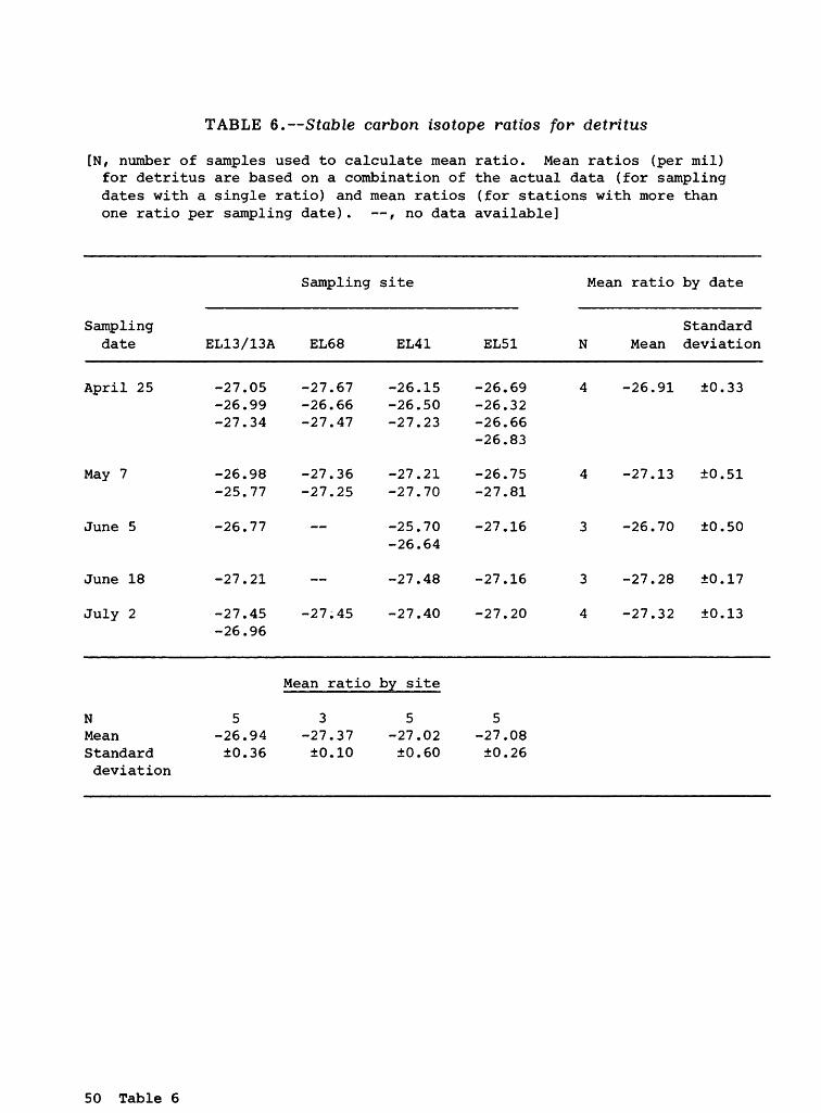
TABLE 6. Stable carbon isotope ratios for detritus

[N, number of samples used to calculate mean ratio. Mean ratios (per mil)for detritus are based on a combination of the actual data (for samplingdates with a single ratio) and mean ratios (for stations with more thanone ratio per sampling date). , no data available]

Sampling date

April 25

May 7

June 5

EL13/13A

-27.05 -26.99 -27.34

-26.98 -25.77

-26.77

Sampling

EL68

-27.67 -26.66 -27.47

-27.36 -27.25

site

EL41

-26.15 -26.50 -27.23

-27.21 -27.70

-25.70 -26.64

EL51

-26.69 -26.32 -26.66 -26.83

-26.75 -27.81

-27.16

Mean ratio by date

Standard N Mean deviation

4 -26.91 ±0.33

4 -27.13 ±0.51

3 -26.70 ±0.50

June 18 -27.21 -27.48 -27.16 3 -27.28 ±0.17

July 2

NMeanStandarddeviation

-27.45 -27.45 -27.40 -27.20 4 -27.32 ±0.13 -26.96

Mean ratio by site

5355-26.94 -27.37 -27.02 -27.08±0.36 ±0.10 ±0.60 ±0.26

50 Table 6

TABLE 7. Stable nitrogen isotope ratios for detritus

[N, number of samples used to calculate mean ratio. Mean ratios (per mil) for detritus are based on a combination of the actual data (for sampling dates with a single ratio) and mean ratios (for stations with more than one ratio per sampling date). , no data available]

Sampling date

April 25

May 7

June 5

June 18

July 2

N Mean Standard deviation

EL13/13A

6.87 7.84 5.14

6.94 9.50 9.76

4.00

7.23

5.16 4.52

5 6.28

±1.89

Sampling

EL68

5.78 6.94

5.79 6.77

6.40

Mean ratio

3 6.35

±0.06

site

EL41

8.29 6.66 8.33

4.71 5.62

4.82

3.09

4.50

by site

5 5.07

±1.70

EL51

4.98 4.32 6.46

6.02 5.85

4.64

4.19

4.19

5 4.84

±0.75

Mean ratio by date


4 6.50 ±1.03

4 6.53 ±1.54

3 4.49 ±0.43

3 4.84 ±2.14

4 4.98 ±0.98

Table 7 51

TABLE 8. Stable carbon isotope ratios for POM <43 ym (phytoplankton)

[N, number of samples used to calculate mean ratio. Mean ratios (per mil) for POM <43 ym (phytoplankton) are based on a combination of the actual data (for sampling dates with a single ratio) and mean ratios (for stations with more than one ratio per sampling date). , no data available, ym, micrometers]

Sampling date

April 25

May 7

June 5

June 18

July 2

August 13

EL13/13A

-25.94 -26.08

-25.04 -26.00

-25.84

-26.06

-26.06 -25.96

-26.74 -25.85 -25.84

Sampling

EL68

-26.44 -26.54

-27.34

-26.93

-25.79

-25.94

-25.90 -25.55

site

EL41

-26.21 -26.22

-25.52

-26.83

-27.20

-26.69

-26.48 -26.08

EL51

-26.47 -26.83

-25.82 -26.33

-26.42

-27.05 -26.34

-26.65

-26.10 -26.21 -26.29

Mean ratio by date


4 -26.34 ±0.28

4 -26.22 ±0.86

4 -26.50 ±0.50

4 -26.44 ±0.64

4 -26.32 ±0.40

4 -26.09 ±0.25

Mean ratio by site


6 -25.93 ±0.22

6 -26.37 ±0.66

6 -26.46 ±0.58

6 -26.45 ±0.26

52 Table 8

TABLE 9. Stable nitrogen isotope ratios for POM <43 ym (phytoplankton)

[N, number of samples used to calculate mean ratio. Mean ratios (per mil) for POM <43 ym (phytoplankton) are based on a combination of the actual data (for sampling dates with a single ratio) and mean ratios (for stations with more than one ratio per sampling date). , no data available, ym, micrometers; <, less than]

Sampling date

April 25

May 7

June 5

June 18

July 2

August 13


EL13/13A

5.65 5.83

5.81 5.65

4.41

4.20

5.41 4.84

5.93 6.50 5.09

6 5.17

±0.72

Sampling

EL68

5.18 5.36

6.69 6.70

5.22

2.55

6.54

5.17 5.92

Mean ratio

6 5.30

±1.49

site

EL41

6.26 6.60

6.21

5.38

4.91

4.08

4.01 6.48

by site

6 5.38

±0.86

EL51

6.07 6.06

7.01 7.53

4.64

4.62 4.83

3.84

5.45 4.98 6.32

6 5.35

±1.22

Mean ratio by date


4 5.88 ±0.49

4 6.48 ±0.66

4 4.91 ±0.46

4 4.10 ±1.07

4 4.90 ±1.23

4 5.55 ±0.24)

Table 9 53

TABLE 10. Stable carbon isotope ratios for POM >43 \im (small zooplankton)

[N, number of samples used to calculate mean ratio. Mean ratios (per mil) for POM >43 ym (small zooplankton) are based on a combination of the actual data (for sampling dates with a single ratio) and mean ratios (for stations with more than one ratio per sampling date). , no data available, ym, micrometers; >, greater than]

Sampling date

April 25

May 7

June 5

June 18

July 2

August 13


EL13/13A

-26.61

-26.62

-26.90

-27.21

-26.53

-26.61

6 -26.75 ±0.26

Sampling

EL68

-27.07

-27.25

-27.07

-26.76

-26.56

-26.95 -26.97

Mean ratio

- 6 -26.94 ±0.24

site

EL41

-27.24 -27.31

-27.35

-27.50

-26.84

-27.03

-27.83 -27.57

by site

6 -27.28 ±0.31

EL51

-26.84 -27.29

-27.61

-27.67

-27.15

-26.96

-27.46 -27.86

6 -27.35 ±0.33

Mean ratio by date


4 -27.01 ±0.28

4 -27.21 ±0.42

4 -27.28 ±0.36

4 -26.99 ±0.22

4 -26.77 ±0.26

4 -27.23 ±0.54

54 Table 10

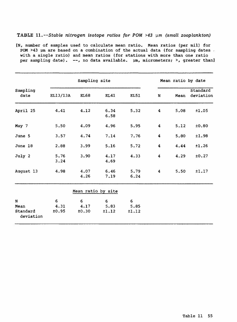
TABLE 11. Stable nitrogen isotope ratios for POM >43 \im (small zooplankton)

[N, number of samples used to calculate mean ratio. Mean ratios (per mil) for POM >43 ym are based on a combination of the actual data (for sampling dates - with a single ratio) and mean ratios (for stations with more than one ratio per sampling date). , no data available. ym, micrometers; >, greater than]

Sampling date

April 25

May 7

June 5

June 18

July 2

August 13


EL13/13A

4.41

5.50

3.57

2.88

5.76 3.24

4.98

6 4.31

±0.95

Sampling

EL68

4.12

4.09

4.74

3.99

3.90

4.07 4.26

Mean ratio

6 4.17

±0.30

site

EL41

6.34 6.58

4.96

7.14

5.16

4.17 4.69

6.46 7.19

by site

6 5.83

±1.12

EL51

5.32

5.95

7.76

5.72

4.33

5.79 6.24

6 5.85

±1.12

Mean ratio by date


4 5.08 ±1.05

4 5.12 ±0.80

4 5.80 ±1.98

4 4.44 ±1.26

4 4.29 ±0.27

4 5.50 ±1.17

Table 11 55

TABLE 12. Stable carbon isotope ratios for large zooplankton

[N, number of samples used to calculate mean ratio. Mean ratios (per mil) for large zooplankton are based on a combination of the actual data (for sampling dates with a single ratio) and mean ratios (for stations with more than one ratio per sampling date). , no data available]

Sampling date

May 7

June 5

June 18

July 2

August 13


EL13/13A

-26.62

-26.23

-26.92 -26.97

-26.82 -27.16

4 -26.70 ±0.36

Sampling

EL68

-29.20

-28.13

-26.42

-28.11

-26.43

Mean ratio

5 -27.66 ±1.21

site

EL41

-27.09

-25.46

-27.54

-28.77

-27.78 -27.83

by site

5 -27.33 ±1.21

EL51

-27.55

-26.98

-28.29

-27.78 -27.91

4 -27.67 ±0.55

Mean ratio by date


4 -27.61 ±1.12

2 -26.80 ±1.89

4 -26.79 ±0.59

4 -28.03 ±0.77

4 -27.27 ±0.68

56 Table 12

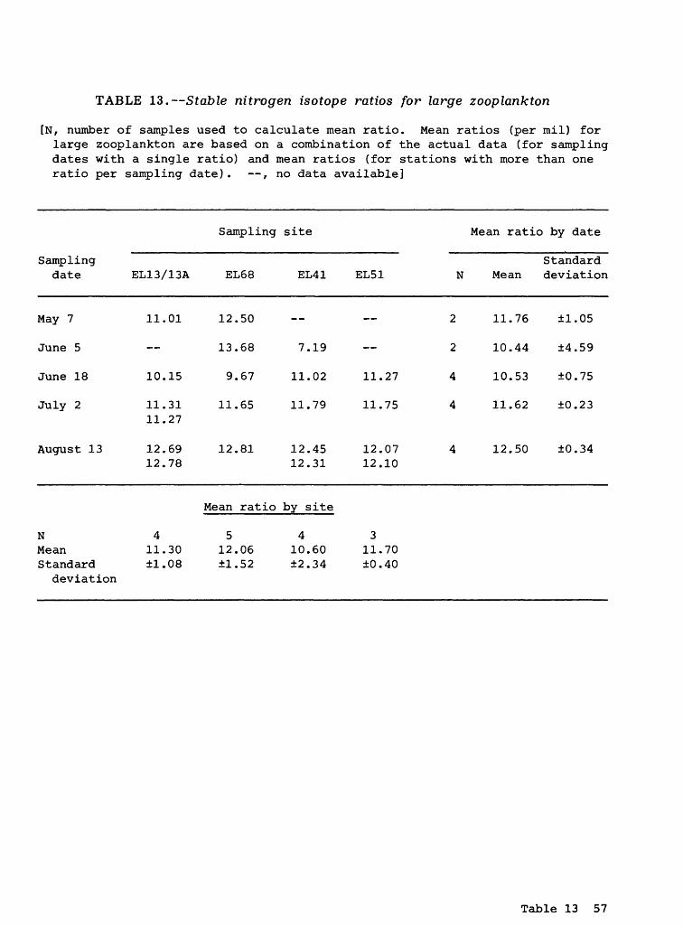
TABLE 13. Stable nitrogen isotope ratios for large zooplankton

[N, number of samples used to calculate mean ratio. Mean ratios (per mil) for large zooplankton are based on a combination of the actual data (for sampling dates with a single ratio) and mean ratios (for stations with more than one ratio per sampling date). , no data available]

Sampling date

May 7

June 5

June 18

July 2

August 13

N Mean Standard

deviation

EL13/13A

11.01

10.15

11.31 11.27

12.69 12.78

4 11.30 ±1.08

Sampling

EL68

12.50

13.68

9.67

11.65

12.81

Mean ratio

5 12.06 ±1.52

site

EL41 EL51

7.19

11.02 11.27

11.79 11.75

12.45 12.07 12.31 12.10

by site

4 3 10.60 11.70 ±2.34 ±0.40

Mean ratio by date


2 11.76 ±1.05

2 10.44 ±4.59

4 10.53 ±0.75

4 11.62 ±0.23

4 12.50 ±0.34

Table 13 57

TABLE 14. Stable carbon isotope ratios for Neomysis shrimp

[N, number of samples used to calculate mean ratio. Mean ratios (per mil) for Neomysis shrimp are based on a combination of the actual data (for sampling dates with a single ratio) and mean ratios (for stations with more than one ratio per sampling date). , no data available]

Sampling date

April 25

May 7

June 5

June 18

July 2

July 12

August 13

EL13/13A

-23.94 -24.88 -22.66

-21.91

-26.80

-24.64 -25.46

-24.23

-24.05 -25.44

Sampling

EL68

-26.94 -27.27

-26.63

-26.79

-24.53

-26.52

-25.06 -23.92

site

EL41 EL51

-26.40 -26.76 -26.84 -26.60

-26.94

-26.62 -26.95

-26.62 -26.36

-26.63 -26.64

-26.81

Mean ratio by date


4 -26.06 ±1.50

3 -25.16 ±2.82

4 -26.79 ±0.13

2 -26.49 ±0.19

4 -25.71 ±1.09

2 -25.38 ±1.62

3 -25.35 ±1.28

Mean ratio by site


6 -24.43 ±1.60

6 -26.01 ±1.18

5 5 -26.69 -26.69 ±0.14 ±0.22

58 Table 14

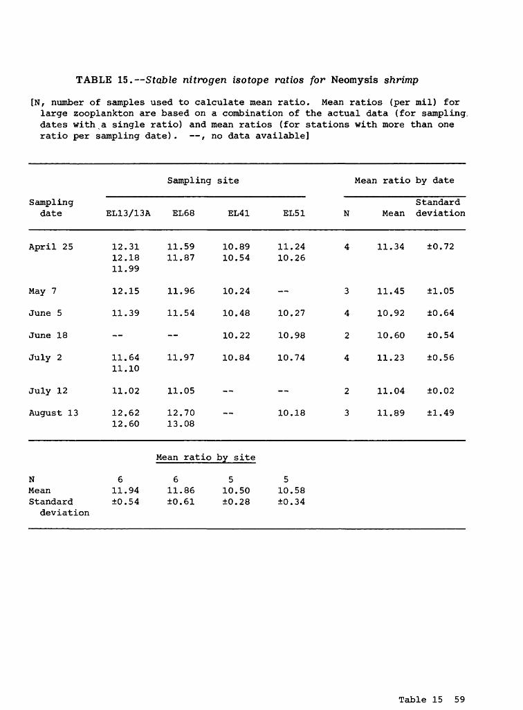
TABLE 15. Stable nitrogen isotope ratios for Neomysis shrimp

[N, number of samples used to calculate mean ratio. Mean ratios (per mil) for large zooplankton are based on a combination of the actual data (for sampling, dates with a single ratio) and mean ratios (for stations with more than one ratio per sampling date). , no data available]

Sampling date

April 25

May 7

June 5

June 18

July 2

July 12

August 13


EL13/13A

12.31 12.18 11.99

12.15

11.39

11.64 11.10

11.02

12.62 12.60

6 11.94 ±0.54

Sampling

EL68

11.59 11.87

11.96

11.54

11.97

11.05

12.70 13.08

Mean ratio

6 11.86 ±0.61

site

EL41 EL51

10.89 11.24 10.54 10.26

10.24

10.48 10.27

10.22 10.98

10.84 10.74

10.18

by site

5 5 10.50 10.58 ±0.28 ±0.34

Mean ratio by date


4 11.34 ±0.72

3 11.45 ±1.05

4 10.92 ±0.64

2 10.60 ±0.54

4 11.23 ±0.56

2 11.04 ±0.02

3 11.89 ±1.49

Table 15 59

TABLE 16. Stable carbon isotope ratios for striped bass

[N, number of samples used to calculate mean ratio. Mean ratios (per mil) for striped bass are based on the actual data. , no data available, mm, millimeters; <, less than; >, greater than]

Site EL13/13A Site EL68

Samplingdate

April 25

June 5

June 18

June 27

July 2

July 12

July 26


Stablecarbon

Length isotope Length(mm) ratio (mm)

__ .. __

__ ..6-12 -25.35 6-12

13-2031-40

13-2021-3031-40

13-20 -27.01 13-20

31-40

6-12 -25.3813-20 -24.4921-30 -23.64

21-3031-40

>40

Mean

<6 mm 6-12 mm

4 7-23.56 -23.25±1.94 ±2.51

Stablecarbonisotoperatio

__

~

.--19.17-23.75-25.15

-24.64-25.33-25.96

-24.40-23.32

-23.27-23.37-24.60

isotope ratio

13-20 mm

5-24.86±1.25

Site EL41

Stablecarbon

Length isotope(mm) ratio

<6 -22.816-12 -20.36

31-40 -25.43

<6 -25.366-12 -24.54

6-12 -24.72

for length of fish

21-30 mm

3-24.08±1.10

Site EL51

Stablecarbon

Length isotope(mm) ratio

<6 -21.186-12 -23.23

._

<6 -24.90

31-40 mm >40 mm

5 1-24.64 -24.60±1.22

60 Table 16

TABLE 17. Stable nitrogen isotope ratios for striped bass

[N, number of samples used to calculate mean ratio. Mean ratios (per mil) for striped bass are based on the actual data. , no data available, mm, millimeters; <, less than; >, greater than]

Site EL13/13A Site EL68 Site EL41 Site EL51

Samplingdate

April 25

June 5

June 18

June 27

July 2

July 12

July 26


Stablenitrogen

Length isotope Length(mm) ratio (mm)

__ __ _

__

6-12 19.38 6-12

13-2031-40

13-2021-3031-40

13-20 13.75 13-20

31-40

6-12 14.2813-20 13.5921-30 13.16

21-3031-40

>40

Mean

<6 mm 6-12 mm

4 718.15 14.77±4.85 ±2.40

Stable Stablenitrogen nitrogenisotope Length isotope Lengthratio (mm) ratio (mm)

<6 17.56 <66-12 16.11 6-12

31-40 13.48

<6 14.56 <612.22 6-12 13.6612.4313.00

12.7912.6113.05

6-12 12.9013.6713.82

13.9113.9113.30

isotope ratio for length of fish

13-20 mm 21-30 mm 31-40 mm

53513.25 13.23 13.45±0.60 ±0.65 ±0.42

Stablenitrogenisotoperatio

25.1714.86

15.31

__

>40 mm

113.30

Table 17 61

TABLE 18. Stable carbon isotope ratios for municipal wastewater- treatment plants

[N, number of samples used tocalculate mean ratio. Mean ratios (per mil) for municipal wastewater- treatment plants are based on the actual data. , no data available]

TABLE 19. Stable nitrogen isotope ratios for municipal wastewater- treatment plants

[N, number of samples used to calculate mean ratio. Mean ratios (per mil) for municipal wastewater- treatment plants are based on the actual data. , no data available]

Wastewater-treatment plantsSampling ______________________

date Sacramento Stockton

Wastewater-treatment plantsSampling _____________________

date Sacramento Stockton

August 28 -24.08 -24.15

-24.10 -24.27

NMean Standard deviation

Mean ratio by site

2 24.12 ±0.08

2-24.19 ±0.12

August 28

NMean Standard deviation

1.602.01

15.5115.07

Mean ratio by site

21.80

±0.29

215.29 ±0.31

62 Tables 18 and 19

Download - Use of Stable Carbon and Nitrogen Isotopes to Trace the Larval

Top Related