
General rights Copyright and moral rights for the publications made accessible in the public portal are retained by the authors and/or other copyright owners and it is a condition of accessing publications that users recognise and abide by the legal requirements associated with these rights.
Users may download and print one copy of any publication from the public portal for the purpose of private study or research.
You may not further distribute the material or use it for any profit-making activity or commercial gain
You may freely distribute the URL identifying the publication in the public portal If you believe that this document breaches copyright please contact us providing details, and we will remove access to the work immediately and investigate your claim.
Downloaded from orbit.dtu.dk on: Feb 26, 2022
Understanding the formation process of the liquid slug in a hilly-terrain wet natural gaspipeline
Yang, Yan; Li, Jingbo; Wang, Shuli; Wen, Chuang
Published in:Journal of Environmental Chemical Engineering
Link to article, DOI:10.1016/j.jece.2017.08.010
Publication date:2017
Document VersionPeer reviewed version
Link back to DTU Orbit
Citation (APA):Yang, Y., Li, J., Wang, S., & Wen, C. (2017). Understanding the formation process of the liquid slug in a hilly-terrain wet natural gas pipeline. Journal of Environmental Chemical Engineering, 5(5), 4220-4228.https://doi.org/10.1016/j.jece.2017.08.010

Accepted Manuscript
Title: Understanding the formation process of the liquid slugin a hilly-terrain wet natural gas pipeline
Authors: Yan Yang, Jingbo Li, Shuli Wang, Chuang Wen
PII: S2213-3437(17)30394-9DOI: http://dx.doi.org/doi:10.1016/j.jece.2017.08.010Reference: JECE 1805
To appear in:
Received date: 19-5-2017Revised date: 7-8-2017Accepted date: 8-8-2017
Please cite this article as:YanYang, JingboLi, ShuliWang,ChuangWen,Understandingthe formation process of the liquid slug in a hilly-terrainwet natural gas pipeline, Journalof Environmental Chemical Engineeringhttp://dx.doi.org/10.1016/j.jece.2017.08.010
This is a PDF file of an unedited manuscript that has been accepted for publication.As a service to our customers we are providing this early version of the manuscript.The manuscript will undergo copyediting, typesetting, and review of the resulting proofbefore it is published in its final form. Please note that during the production processerrors may be discovered which could affect the content, and all legal disclaimers thatapply to the journal pertain.

Understanding the formation process of the liquid slug in a hilly-terrain wet
natural gas pipeline
Yan Yang1, 2, Jingbo Li1, Shuli Wang1, Chuang Wen2,*
1School of Petroleum Engineering, Changzhou University, Zhonglou District,
Changzhou, Jiangsu 213016, China
2Department of Mechanical Engineering, Technical University of Denmark, Nils
Koppels Allé, 2800 Kgs. Lyngby, Denmark
*Corresponding author. Tel.: +45 4525 4168; fax: +45 4525 1961. E-mail address:
[email protected] (C. Wen).

Abstract: In the present work, the liquid slug formation in a hilly-terrain pipeline is
simulated using the Volume of Fluid model and RNG k-ε turbulence model. The
numerical model is validated by the experimental data of the horizontal slug flow. The
influence of the pipe geometric structure and flow condition on the liquid slug
formation is discussed including pipe diameter, inclination angle, gas superficial
velocity and liquid holdup. The results show that the pipe is blocked by the liquid slug
at the moment of slug formed. The pipe pressure suddenly increases, and then
decreases gradually in the process of liquid slug formation and motion. The pipe
pressure drop and liquid holdup decrease along with the increasing inclination angle
of ascending pipe. On the contrary, they rise with the increase of the inclination angle
of descending pipe. Higher gas superficial velocity and liquid holdup result in a larger
pressure drop in the formation of a liquid slug, and correspondingly induces a slug
flow more rapidly in the hilly-terrain pipelines.
Key words: liquid slug; pipe diameter; inclination angle; gas superficial velocity;
liquid holdup
Nomenclature
C1 [-] constant
C2 [-] constant
D [mm] pipe diameter
F [N] external body force

Fvol [N] surface force
Gb [-] generation of turbulence kinetic energy due to buoyancy
Gk [-] generation of turbulence kinetic energy due to mean
velocity gradients
g [m/s2] acceleration of gravity
h [mm] the level of stagnant liquid
k [m2s-2] turbulent kinetic energy
L [m] pipeline length
pqm [-] the mass transfer from phase p to phase q
qpm [-] the mass transfer from phase q to phase p
n [-] surface normal
n̂ [-] unit normal
p [Pa] pressure
Q [m3s-1] volume of pipe
QL [m3s-1] volume of stagnant liquid
Rε [-] additional term.
Saq [-] source term
Sk [-] source term
S [-] source term
t [s] time
u [ms-1] velocity
VG [ms-1] inlet gas velocity

VSL [ms-1] superficial liquid velocity
VSG [ms-1] superficial gas velocity
YM [-] contribution of the fluctuating dilatation in compressible
turbulence to the overall dissipation rate
Greek letters
α [-] volume fraction
αk [-] constant
αε [-] constant
β [-] constant
[-] turbulent dissipation rate
δij [-] Kronecker delta
μ [m2s-1] dynamic viscosity
[kgm-3] density
θ [°] inclination angle of pipe
θ1 [°] inclination angle of descending pipe
θ2 [°] inclination angle of ascending pipe
κ [-] defined in terms of the divergence of the unit normal

1 Introduction
The natural gas field usually locates in hilly or basin region, and then the
hilly-terrain pipelines are used inevitably. The wet gas transportation approach is
widely used in gathering transport system for gas field. The water in wet gas can
assemble in the low-lying pipes, and becomes stagnant liquid in the process of
transporting wet gas. It leads to the formation of the liquid slug or the slug flow,
which can cause a shapely pressure and liquid holdup (liquid volume fraction)
fluctuation in the pipeline system. The intermittent stress in the pipelines can affect
the normal operation, accelerate the corrosion problem and even damage the
transporting equipment [1-3]. Therefore, it is important to study and predict the slug
flow in the hilly-terrain pipelines.
For the slug flow, the study mainly focuses on the horizontal pipe, vertical pipe
and hilly-terrain pipes. For the horizontal pipelines, Kordyban and Ranov [4]
introduced a classic Kelvin-Helmholtz instability theory to explain the mechanism of
the slug formation. They found that the slug formed when the wave length formed in
the gas - liquid surface was greater than the height of gas space. Woods and Hanratty
[5] proposed an approach to predict the stability of liquid slug whether it is
determined by the volume flow in and out of the slug. A prediction method based on
one-dimensional two-fluid model was presented for predicting hydrodynamic slug
initiation and growth by Issa and Kempf [6]. The approach was used for the numerical
simulation in horizontal, inclined and V-section pipes, and the numerical results were
compared with the experimental data. Al-Safran [7] developed a predictive empirical

correlation for predicting slug frequency in gas-liquid two-phase horizontal pipes. For
reducing predictive, a Poisson probability model was proposed to predict slug
frequency in gas-liquid pipes [8]. Al-Safran et al. [9] then proposed a new empirical
relationship to predict slug liquid holdup in high viscosity liquids. The new empirical
relationship showed a better capability than the low viscosity empirical relationship
because the viscosity term was included in the new model.
For the studies of a slug in the vertical pipelines, Clarke and Issa [10] presented a
numerical model to predict a single Taylor bubble velocity in the vertical tubes using
the ensemble average transport equations and k-ε turbulence model. Taha and Cui [11]
used the Volume of Fluid (VOF) model to simulate the motion of a single Taylor
bubble in the vertical tubes and obtained the shape and flow parameters of the slug.
Mayor et al. [12] carried out an experiment for slug flow in a vertical pipe by
employing a non-intrusive image analysis technique and proposed a correlation for
the bubble-to-bubble interaction. Abdulkadir et al. [13] conducted the experimental
and numerical studies in the vertical pipes with 6 m long and 0.067 m internal
diameter. The computational results were reasonably in good agreement with the
experimental data.
Zheng et al [14] developed a slug-tracking model to track the behavior of a slug,
including the slug generation, dissipation, shrink and grow in hilly-terrain pipelines.
Henau and Raithby [15] investigated the slug behavior in two-phase pipes which
contained several uphill and downhill sections. Al-Safran et al. [16] carried out
several experiments in a 420 m long smooth steel pipe flow loop which included a

hilly-terrain test section and found five possible flow behavior categories in
hilly-terrain section. Ersoy et al. [17] investigated gas-oil-water three-phase slug flow
in hilly-terrain pipelines and obtained the flow characteristics of a slug.
The studies on the gas-liquid slug flow are mainly focused on the horizontal and
vertical pipelines. However, the formation and motion of a single liquid slug still need
to be further studied in hilly-terrain pipelines, in particular the existence of the
stagnant liquids. In this paper, the numerical study is carried out to understand the
formation process of a single liquid slug in hilly-terrain pipelines. The influence of
geometric structure and flow conditions on liquid slug formation is analyzed in detail,
including the pipe diameter, inclination angle, gas superficial velocity and liquid
holdup.
2 Mathematical model
The slug flow is a sort of complex gas-liquid two-phase flow, which has a
distinct phase interface. The interface catching is a key step for the simulation of the
liquid slug. The VOF model is a kind of surface-tracking technology based on the
fixed Eulerian mesh and it can be used for modeling two or more immiscible fluids.
Therefore, the VOF model is employed here to track the gas-liquid phase interface in
hilly-terrain pipelines. In addition, the turbulence model is necessary due to the fact
that the flow is turbulent in our simulation.
2.1 Governing equations
Continuity equation [18]:

( ) 0i
i
ut x
(1)
Momentum equation [19]:
The momentum equation is solved throughout the computational domain, and the
resulting velocity field is shared among all the phases.
( ) ( ) ( )T
u uu p u u g Ft
(2)
where is the density, u is the velocity, p is the static pressure, is the dynamic
viscosity, g is the gravitational body force and F is an external body force, t is
the time.
2.2 Volume fraction equation
The volume fraction of each phase in each grid cell is calculated throughout the
domain. The interface between two phases is tracked by solving the continuity
equation for the volume fraction of one (or more) of the phases. The volume fraction
equation is as follows [20]:
1
1( ) ( ) ( )
q
n
q q q q q a pq qp
pq
a a u S m mt
(3)
where pqm is the mass transfer from phase q to phase p and qpm is the mass
transfer from phase p to phase q, αq is the volume fraction of phase q, q
S is the
source term.
2.3 Continuum surface force model
The effect of surface force along the interface is included in the VOF model. The
continuum surface force (CSF) model proposed by Brackbill et al. [21] is used in this
paper. It is implemented as a source term in the momentum equation. The surface

force volF is expressed as follows:
1
2
i ivol ij
i j
F
(4)
where σij is the surface tension coefficient between phase i and j, αi is the volume
fraction of phase i, ρi and ρj is the density of phase i and j. ρ is the volume-averaged
density computed by Eq. (5):
2 2 2 1(1 ) (5)
The curvature, κ, is defined in terms of the divergence of the unit normal, n̂ :
n̂ (6)
where
ˆn
nn
(7)
qn (8)
where n is the surface normal, defined as the gradient of the αq.
2.4 Turbulence model
Depending on the information required, different turbulence models can be
applied, from k-ε model, shear stress transport model, large eddy simulation to direct
numerical simulation [22-24]. Among these models, the RNG k-ε turbulence model
employs an additional term in its dissipation rate equation that can improve the
accuracy for rapidly strained flow. It is more suitable for simulating large curvature
and strain rate flow. The RNG k-ε turbulence model is employed here because the
flow turns at the elbow of the pipe which connects the uphill section and downhill
section in hilly-terrain pipelines. The turbulence kinetic energy, k, and its rate of

dissipation, ε, are as follows [25]:
( )( ) ik eff k b M k
i j j
kuk kG G Y S
t x x x
(9)
2
12
( )( ) ieff k
i j j
u CG C R S
t x x x k k
(10)
where μeff is the effective eddy viscosity. Gk is the generation of turbulence kinetic
energy due to the mean velocity gradients; Gb represents the generation of turbulence
kinetic energy due to buoyancy; YM represents the contribution of the fluctuating
dilatation in compressible turbulence to the overall dissipation rate. Rε is the
additional term. The quantities αk and αε are the inverse effective Prandtl numbers for
k and ε, respectively. Sk and S are the source terms. The C1ε and C2ε are constants.
3 Numerical schemes
3.1 Geometric model
The sketch of the hilly - terrain pipeline is shown in Figure 1. This pipeline
contains a descending pipe and an ascending pipe, respectively. The inclination angles
of two pipes are θ1 and θ2. The stagnant liquid is water and the gas phase is methane.
Two pressure monitoring points (P1 and P2) are set at the center of the pipe cross
section which locates in x = -15 D and x = 15 D. The pipe pressure drop is the value
of 1 2P P in this paper.
The hilly-terrain pipe model includes a downhill section and an uphill section, as
shown in Figure 2. The pipe diameter is defined as D and the length of every section
is 50 D to ensure a fully developed flow
3.2 Mesh generation
The computational domain should be meshed after the geometric model is
established. The commercial software ANSYS ICEM CFD is selected as the meshing
tool. The hexahedral mesh and O-block technology is selected as the grid partition
strategy for improving the quality of the grid. The grid system is shown in Figure 3.
The computational grid of 317,760 hexahedral cells is employed for the simulation
after the grid independent tests.
3.3 Numerical method
The simulation is achieved in commercial software ANSYS Fluent. The VOF
multiphase model and the RNG k-ε turbulence model are applied for tracking the
gas-liquid phase interface. The boundary conditions of pipe inlet and outlet are
defined as the velocity-inlet and the outflow, respectively. The wall condition is set to
be frictionless with no slipping [26]. The operating pressure is 0 Pa and the reference
pressure location is set at the center point of pipe outlet. The Pressure-Velocity
coupling scheme is performed with the PISO approach. The QUICK scheme is
implemented for discretizing continuity equation, momentum equation and turbulence
equation. The Geometric Reconstruction scheme (Geo-Reconstruct) is chosen for the
volume fraction equation. The time step size is 0.0001 s for proving calculation
convergence in every time step.
4 Results and discussion
4.1 Model validation and verification
In this paper the experimental data obtained by Heywood and Richardson [27]

are employed to validate our numerical method. The experiments were carried out in
an air-water flow loop system, which included a horizontal pipeline of 42 mm inner
diameter. The γ-ray absorption method was used to measure the slug liquid holdup.
Six experimental data in the same superficial liquid velocity (0.978 m/s) were selected
for the model validation in different superficial gas velocities. The results of the
comparison between the experimental and numerical data are shown in Figure 4. It
shows that the maximum relative error is 5.9% in superficial gas velocity of 4.145 m/s.
Therefore, the numerical results are in good agreement with the experimental data.
The mesh quality is an important factor in numerical simulation. The appropriate
mesh size can ensure the accuracy of calculation by taking into account the
computational efficiency. The grid independence is tested in three cells number of
about 180,000, 380,000 and 780,000, respectively. The pressure drop calculated with
different cells is shown in Figure 5. It shows that the computed results with 180,000
grid cells are much different from other two cases. The difference of the pressure drop
between 380,000 and 780,000 cells is tiny. Therefore, the numerical simulation is
performed with 380,000 cells considering the computational accuracy and efficiency.
4.2 Liquid slug formation process
Figure 6 shows the formation process of a liquid slug in the 150 mm diameter
pipe with the inclination angle of θ2 = θ2 = 5°. The inlet gas velocity is 6.5 m/s, and
the ratio of the stagnant liquid height, h, to the pipe diameter is 0.75 (h/D=0.75). The
phase fraction distribution with different moment (t) is described in the contours. The
blue region represents the gas phase, while the red one represents the liquid phase.

The axis, x is the position coordinates of pipe along the flow direction.
The flow area decreases due to the stagnant liquid accumulated at the bottom of
hilly-terrain pipes, which cause the increase of the gas velocity. This flow structure
further induces the decline of the pressure above the liquid level. Then suction force is
generated in the vertical upward, which destroys the stability of the gas-liquid
interface. For this reason, a wave crest forms. When the liquid level uplifts to the
top of the pipe and blocks the entire pipe cross section, the liquid slug flow finally
appears (t=0.005 s -0.100 s in Figure 6). The liquid slug then goes into the next
process of moving forward under the pressure difference between the upstream and
downstream of the slug flow (t=0.105-0.120 s in Figure 6).
4.3 Effect of pipe diameter
In this section, the influence of the pipe diameter on the formation of a liquid
slug is discussed in detail. The pipe diameters are 90 mm, 120 mm, 150 mm, 180 mm
and 210 mm, respectively. The length of the ascending and descending pipes is 50 D,
while the inclination angle is set to be 5°. The numerical simulation is implemented in
the identical condition which the inlet gas velocity is 6.5 m/s with h/D=0.75.
Figure 7 shows the pressure curves of point P1 and P2 with the flow time in
different pipe diameters. It shows that the pressure nearly maintains a constant value
at point P2, while fluctuates sharply at point P1. Moreover, the pressure increases
suddenly and then declines slowly at point P2. The reason is that the flow area of the
gas phase decreases gradually because of the pressure fluctuation during the
formation process of the liquid slug. The liquid slug then moves under the pressure

difference between its upstream and downstream flow.
The pressure drops in different pipe diameter at the moment of slug formed are
shown in Figure 8. The pressure drop increases along with the pipe diameter. The
pressure drop ranges from 40,000 Pa to 82,000 Pa. The rate of increasing pressure
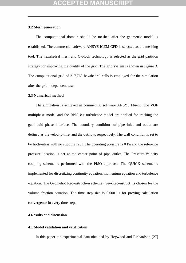
drop is about 30% with the pipe diameter from 90 mm to 210 mm. Figure 9 describes
the slug liquid holdup in different pipe diameters. We can see that the liquid holdup
increases slowly in the pipe diameters from 90 mm to 180 mm, while it declines
slightly in the 210 mm diameter pipe. However, the value of slug liquid holdup
distributes by approximately 0.5 in the entire pipe diameters.
4.4 Effect of pipe inclination angle
The pipe inclination angle plays an important role in the slug formation in hilly
terrain pipelines. The effects of the inclination angle of ascending and descending
pipes are analyzed in this section. The pipe diameter is 150 mm and the inclination
angle are 3°, 5°, 8°, 10° and 12°, respectively. The inlet gas velocity is 6.5 m/s and
the ratio of the stagnant liquid volume (QL) at the bottom of the pipe to the volume of
pipe (Q) is a fixed value.
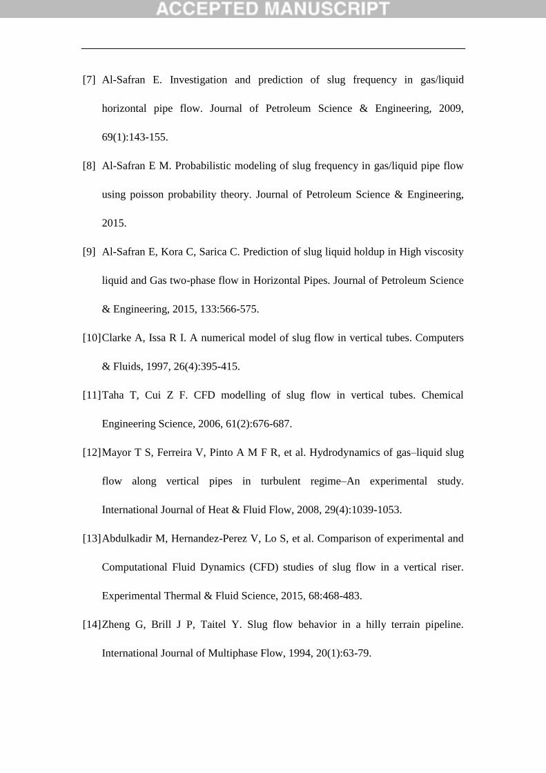
The pressure drop and liquid holdup in different ascending angles with the
descending angle of 3° are shown in Figure 10 and Figure 11, respectively. It can be
seen that the pressure drop declines with the increasing ascending angle. The pressure
drop reduces the maximum about 37.5%, when the ascending angle changes from 3°
to 5°. The change trend of the liquid holdup is similar to the pressure drop that it
decreases with the increasing ascending angle. The liquid holdup at the high

ascending angle of 12° is only 0.35, reducing 40% compared to the one at the lower
ascending angle of 3°.
The pressure drop and liquid holdup in different descending angles are shown in
Figure 12 and Figure 13, respectively, when the ascending angle is fixed at 5°. The
pressure drop and liquid holdup have the similar relationship that they both increase
with the increasing descending angle. The pressure drop ranges from 17,000 Pa to
138,000 Pa, while the liquid holdup changes from 0.35 to 0.57. The maximum
presusre drop appears in the descending angle from 10° up to 12°. However, the
maximum liquid holdup presents in the descending angle from 5° to 8°.
4.5 Effect of gas superficial velocity and liquid holdup
Figure 14 shows the effect of the gas superficial velocity on the pressure drop
during the formation of liquid slug flow under different liquid holdups. We can see
that the increasing gas superficial velocity induces a larger pressure drop in the same
liquid holdup, h/D. The reason is that the greater gas superficial velocity can carry
more liquids, which results in more loss of the kinetic energy during the formation of
liquid slug. It correspondingly determines the higher rise of the gas pressure in the
upstream of the slug. Moreover, in the higher liquid holdup, the increase of the gas
superficial velocity induces a sharper increase of pressure drop. In the conditions of h
/ D = 0.6, USG = 2.5 ~ 4.5 m / s and h / D = 0.65, USG = 2.5 ~ 3.5 m / s, the pipeline
pressure drop is 0 Pa because there is no slug flow in the hilly pipelines.
The change of the gas superficial velocity at the pipe inlet also affects the phase
distribution of the gas-liquid two-phase flows. Figure 15 shows the gas-liquid

two-phase distribution in the same liquid holdup under the conditions of USG=3.5 m/s
and USG=5.5 m/s. From the time point of view, the formation of the liquid slug is
faster with a larger gas superficial velocity. From the figures at USG=3.5 m/s, t=0.20 s,
and USG=5.5 m/s, t=0.12, it can be seen that more liquids are lifted to the top to block
the pipeline as a result of larger gas superficial velocity during the formation of liquid
slug, leading to higher fluctuations of the liquid level. During the growth process of
liquid slug flow, such as in the figures of USG=3.5 m/s, t=0.20 s~0.52 s and USG=5.5
m/s, t=0.12 s~0.40 s, the throwing phenomenon of the slug flow becomes more
obvious that more liquids are reeled into the liquid slug by the slug head, which
makes that both of the length of the slug head and slug body are greater than those in
a smaller gas superficial velocity. This is because the liquid slug body can obtain
higher kinetic energy driven by the upstream natural gas with a larger gas superficial
velocity, which strengthens the ability of the slug to entrain the liquids ahead.
Figure 16 describes the gas-liquid two-phase distribution at different liquid level
of h/D=0.65 and h/D=0.85. For example, the liquid slug forms in a shorter time under
the condition of h/D=0.85. Compared to the phase distributions of h/D=0.65 and
h/D=0.85, we can conclude that higher liquid level is easier to induce the formation of
the liquid slug. Moreover, more liquids are carried by the gas phase during the
formation of the liquid slug in higher liquid level, resulting in more serious blocking
in the pipeline. The throwing phenomenon of the slug head at h/D=0.85 is much more
serious than that of h/D=0.65, which also leads to longer slug head and slug body in
higher liquid level. When the liquids are thrown out of the slug head, the slug body

gradually reduces until the slug disappears.
5 Conclusions
The VOF and RNG k-ε turbulence models show the reasonable results in
simulating the formation process of a liquid slug. The validation of the numerical
model and mesh independence test are examined in this paper. The distinct gas-liquid
two-phase distribution and the formation process of a liquid slug are obtained by
numerical simulation in different pipe geometric parameters. The pipe cross-section is
blocked by the liquid phase at the moment of a liquid slug formed. The pressure
suddenly increases, and then declines gradually in process of liquid slug formation
and motion. The pipe diameter has a tiny effect on the slug formation, since the
pressure drop and the liquid holdup change little. When the inclination angle of the
pipe varies, the similar trend occurs both for pipe pressure and liquid holdup. The
pressure drop and liquid holdup decline with the increase of the ascending angle. On
the contrary, they rise along with the increasing descend. It indicates that the
inclination angle of a pipe is a key influence factor for the liquid slug formation. The
increase of the gas superficial velocity and liquid holdup both causes the rise of the
pressure drop, and correspondingly induces the formation of liquid slug in a shorter
time.
Acknowledgements
This work was supported by the National Natural Science Foundation of China
(51444005, 51606015, 51574045), the Natural Science Foundation of Jiangsu

Province, China (BK20150270), and the General Program of Natural Science
Research Project of Jiangsu Province Universities and Colleges (15KJB440001). The
research leading to these results has received funding from the People Programme
(Marie Curie Actions) of the European Union's Seventh Framework Programme
(FP7/2007-2013) under REA grant agreement no. 609405 (COFUNDPostdocDTU).
References
[1] Yang Y, Li Z, Wen C. Effects of alternating current on X70 steel morphology and
electrochemical behavior. Acta Metallurgica Sinica, 2013, 49(1): 43-50.
[2] Wen C, Li J, Wang S, Yang Y. Experimental study on stray current corrosion of
coated pipeline steel. Journal of Natural Gas Science and Engineering, 2015, 27:
1555-1561.
[3] Yang Y, Wang S, Wen C. Experimental study on alternating current corrosion of
pipeline steel in alkaline environment. International Journal of Electrochemical
Science, 2016, 11: 7150-7162.
[4] Kordyban E S, Ranov T. Mechanism of slug formation in horizontal two-phase
flow. Journal of Fluids Engineering, 1970, 92(4):857-864.
[5] Woods B D, Hanratty T J. Relation of slug stability to shedding rate. International
Journal of Multiphase Flow, 1996, 22(22):809-828.
[6] Issa R I, Kempf M H W. Simulation of slug flow in horizontal and nearly
horizontal pipes with the two-fluid model. International Journal of Multiphase
Flow, 2003, 29(1):69-95.
[7] Al-Safran E. Investigation and prediction of slug frequency in gas/liquid
horizontal pipe flow. Journal of Petroleum Science & Engineering, 2009,
69(1):143-155.
[8] Al-Safran E M. Probabilistic modeling of slug frequency in gas/liquid pipe flow
using poisson probability theory. Journal of Petroleum Science & Engineering,
2015.
[9] Al-Safran E, Kora C, Sarica C. Prediction of slug liquid holdup in High viscosity
liquid and Gas two-phase flow in Horizontal Pipes. Journal of Petroleum Science
& Engineering, 2015, 133:566-575.
[10] Clarke A, Issa R I. A numerical model of slug flow in vertical tubes. Computers
& Fluids, 1997, 26(4):395-415.
[11] Taha T, Cui Z F. CFD modelling of slug flow in vertical tubes. Chemical
Engineering Science, 2006, 61(2):676-687.
[12] Mayor T S, Ferreira V, Pinto A M F R, et al. Hydrodynamics of gas–liquid slug
flow along vertical pipes in turbulent regime–An experimental study.
International Journal of Heat & Fluid Flow, 2008, 29(4):1039-1053.
[13] Abdulkadir M, Hernandez-Perez V, Lo S, et al. Comparison of experimental and
Computational Fluid Dynamics (CFD) studies of slug flow in a vertical riser.
Experimental Thermal & Fluid Science, 2015, 68:468-483.
[14] Zheng G, Brill J P, Taitel Y. Slug flow behavior in a hilly terrain pipeline.
International Journal of Multiphase Flow, 1994, 20(1):63-79.

[15] Henau V D, Raithby G D. A study of terrain-induced slugging in two-phase flow
pipelines. International Journal of Multiphase Flow, 1995, 21(97):365–379.
[16] Al-Safran E, Sarica C, Zhang H Q, et al. Investigation of slug flow characteristics
in the valley of a hilly-terrain pipeline. International Journal of Multiphase Flow,
2005, 31(3):337-357.
[17] Ersoy G, Sarica C, Al-Safran E, et al. Experimental investigation of three-phase
gas-oil-water slug flow evolution in hilly-terrain pipelines. SPE Annual Technical
Conference and Exhibition. Society of Petroleum Engineers, 2011.
[18] Wen C, Cao X, Yang Y, Li W. An unconventional supersonic liquefied
technology for natural gas. Energy Education Science and Technology Part A:
Energy Science and Research. 2012, 30(1): 651-660.
[19] Wen C, Cao X, Yang Y, Feng Y. Prediction of mass flow rate in supersonic
natural gas processing, Oil & Gas Science and Technology, 2015, 70(6):
1101-1109.
[20] Hirt C W, Nichols B D. Volume of fluid (VOF) method for the dynamics of free
boundaries. Journal of Computational Physics, 1981, 39(1): 201-225.
[21] Brackbill J U, Kothe D B, Zemach C. A continuum method for modeling surface
tension[J]. Journal of computational physics, 1992, 100(2): 335-354.
[22] Yang Y, Walther J H, Yan Y, Wen C. CFD modelling of condensation process of
water vapor in supersonic flows. Applied Thermal Engineering, 2017, 115:
1357-1362.

[23] Yang Y, Li A, Wen C. Optimization of static vanes in a supersonic separator for
gas purification. Fuel Processing Technology, 2017, 156: 265-270.
[24] Yang Y, Wen C. CFD modeling of particle behavior in supersonic flows with
strong swirls for gas separation. Separation and Purification Technology, 2017,
174: 22-28.
[25] Yakhot V, Orszag S A. Renormalization-group analysis of turbulence. Physical
Review Letters, 1986, 57(14): 1722.
[26] Haghighi M, Hawboldt K A, Abdi M A. Supersonic gas separators: review of
latest developments. Journal of Natural Gas Science and Engineering, 2015, 27:
109-121.
[27] Heywood N I, Richardson J F. Slug flow of air-water mixtures in a horizontal
pipe: determination of liquid holdup by γ-ray absorption. Chemical Engineering
Science, 1979, 34(1):17-30.

Figure 1 Sketch of the hilly-terrain pipeline
Figure 2 Computational domain
Figure 3 Mesh characteristic

Figure 4 Comparison between experimental and numerical results in a horizontal pipe
Figure 5 Pressure drop in different cell numbers

Figure 6 Formation process of a liquid slug

Figure 7 Pressure at point P1 and P2 in different pipe diameters
Figure 8 Influence of pipe diameter on pressure drop at the moment of slug formed
Figure 9 Influence of pipe diameter on liquid holdup at the moment of slug formed
Figure 10 Pressure drop in different ascending angle at the moment of slug formed

Figure 11 Liquid holdup in different ascending angle at the moment of slug formed
Figure 12 Pressure drop in different descending angle at the moment of slug formed

Figure 13 Liquid holdup in different descending angle at the moment of slug formed
Figure 14 Pressure drop in different gas superficial velocity and liquid holdup

Figure 15 Gas-liquid two-phase distribution in different gas superficial velocity

Figure 16 Gas-liquid two-phase distribution in different liquid holdup


