Unconventional Monetary Policy and U.S. Housing Markets Dynamics
Yao-Min Chiang National Taiwan University
Email: [email protected]
Jarjisu Sa-Aadu University of Iowa
Email: [email protected]
James D. Shilling DePaul University
Email: [email protected]
March 23, 2015
Abstract
This study investigates whether the unprecedented liquidity injected in the economy by the U.S Fed through unconventional monetary policy measure, popularly known as quantitative easing (QE), is a systematic factor that can explain the abnormally low U.S. housing starts of recent years. We use housing and mortgage markets data that should capture the liquidity induced by QE to construct four unobservable aggregate liquidity factors as key channels through which QE stimulus effects might have been transmitted to housing and mortgage markets. Using monthly MSA level data, we find that expected housing starts are related across time to fluctuations in the aggregate liquidity factors. Specifically, we find that housing starts liquidity betas, their sensitivities to liquidity shocks from QE transmitted through the aggregate liquidity factors significantly influence the level of U.S. investments in new single family housing between 2005 and 2012. However, we find evidence of heterogeneity in the responsiveness of housing starts to innovations in the aggregate liquidity factors in that market regimes with high levels of land use control (constrained markets) exhibit relatively muted sensitivities to fluctuations in the aggregate liquidity factors induced by QE. Remarkably, we also find that in the absence of GSE and FHA capital market activities that channel credit into housing market the contraction in housing starts would have been worse. Further, a build-up in single family homes-for-rent, shadow vacancy liquidity risk, exerts a down-ward pressure on investments in new single family housing.
JEL Classification: E52, E58, R20, R30
Keywords: Unconventional Monetary Policy, Housing Starts, Aggregate Liquidity Factors, Housing Markets
.
1

1:0 Introduction
In the wake of the recent financial crisis triggered by the deterioration in the subprime
mortgage market, the U.S. Federal Reserve was compelled to implement unconventional
monetary policy measures never before used in its history to stabilize financial markets and
stimulate real economic activity. The program became the policy measure of necessity for dealing
with the severe adverse consequences of the crisis when the conventional monetary tool, Federal
Funds rate, reached its zero lower bound (ZLB). At this point unconventional monetary measures
became the only means available to the Fed for managing expectations of the future path of
interest rates and reducing term premium. Although there were several policy measures, the
Fed’s large scale asset purchase (LSAP), popularly known as quantitative easing (QE), is striking
in terms of its unprecedented scale, visible impact on the Fed’s balance sheet and the uncertainty
surrounding its potential impact on financial markets and the real economy. QE involved
purchases of high grade financial assets by the Fed including mortgage backed securities (MBS)
issued by housing-related government sponsored agencies (GSEs), agency debt obligations, and
coupon paying Treasury securities. Since the inception of the program in December 2008, the
Fed has implemented four waves of QE that have caused the Fed’s balance sheet to burgeon from
about $850 billion in 2008 to more than $4.4 trillion as of September 2014 (see Exhibit 1).
Although policy makers were in general supportive of the QE program they nevertheless
expressed some doubt regarding its efficacy as revealed in the following summary of the
December 2008 Federal Open Market Committee (FOMC) on QE1: “The available evidence
indicated [LSAP] purchases would reduce yields on those instruments, and lower yields on those
securities would tend to reduce borrowing costs for a range of private borrowers, although
participants were uncertain as to likely size of such effects”. Indeed, the dramatic impact of the
program on the size of the Fed’s balance sheet led to widespread discomfort among many
economists and policymakers resulting in considerable diversity of opinion regarding the use of
QE and other unconventional tools to stabilize financial markets and stimulate the economy.
The controversy and uncertainty surrounding the efficacy of QE have spawned a growing
literature seeking to uncover the effects of the program on financial markets and the real
economy. 1 Thus far the weight of the empirical evidence has been on the impact of QE on
1 See for example Baumeister and Benati (2010), D’Amico and King (2013), Doh (2010), Gabriel and Lutz (2014), Gagnon, et al. (2011), Hamilton and Wu (2010) , Hancock and Passmore (2011), Krishmamurthy and Vissing-Jorgensen (2011), Strobel and Taylor (2009), Williams (2011) and Wright (2011)
2
financial markets and not on real economic activity. Specifically, the evidence suggests that the
program (in particular QE1) has significantly reduced the general level of long term interest rates,
from which some studies infer that QE must also have stimulated real economic activity. 2
Nevertheless, the precise channel through which the impact of QE may have been transmitted to
real economic activity and the magnitude of the effect are still issues subject to debate. Recently,
attention has shifted to assessing the effect of QE on aggregate output (e.g. Gabriel and
Lutz(2014), Gambacorta, et al (2012), Chung et al 2011, Gertler and Karadi 2012, Kapetanios et
al 2012, and Lenza et al 2011). These papers have generally concluded that QE increased
aggregate economic activity as measured by a peak increase in real output. Additionally, Gertler
and Kanadi (2012) conclude that QE reduce the yield-to-maturity of private securities such as
agency MBS much more than the drop in the yield on Treasury and that this reduction is key for
the transmission of QE stimulus effects to the real economy. 3 Clearly these papers have
advanced our understanding of the likely effects of QE on aggregate economic activity, although
their focus is not on a specific economic activity.
Against this backdrop, this paper investigates whether the aggregate liquidity injected in the
economy by the U.S Federal Reserve through QE is a systematic factor for explaining the
abnormally low housing starts of recent years. Using housing and mortgage markets data that
should capture the stimulus effects of QE and the methodology of principal component analysis
(PCA), we construct four unobservable aggregate liquidity factors – funding liquidity, market
liquidity, credit availability and shadow vacancy, as key channels through which the stimulus
effects of QE might have been transmitted to boost housing starts. The aggregate liquidity factors
are defined as follows: market liquidity is the ease with which an asset such as housing can be
traded, funding liquidity is the ease/cost with which a household and an economic agent such as a
homebuilder can obtain funding, and credit availability refers to availability of credit in mortgage
markets induced by QE via GSEs’ capital market activities and FHA loans. The fourth liquidity
risk factor, shadow vacancy, is designed to capture the attendant liquidity risk of the inventory of
2 QE1 which involved a $100 billion per month purchase of residential mortgage backed securities (RMBS ) and other debt securities issued by government sponsored agencies (Fannie and Freddie) and Treasury securities has been the largest of all the QEs totaling about $17 trillion, lasted 17 months and is generally considered to be the most effective of all the QEs.
3 According to Gertler and Karadi (2012), the transmission channel to real output is LSAPs’ ability to reduce excess return which causes asset prices to rise, which in turn induces investment spending. They further stress that the key to identifying this channel from their simulation of their model rests on the assumption that LSAP is equivalent to central bank intermediation with limits to arbitrage in private intermediation.
3
single-family homes for rent that may eventually be “flipped”, a phenomenon that developed in
housing markets during the recent crisis. 4 We view this development as manifestation of a lack
of transaction intensity, and as such a state variable in housing markets.
We specify and estimate a simple econometric model of investments in new single-family
housing that incorporates standard observable factors that have been shown to influence housing
starts, as well as the relation between housing starts and the four aggregate liquidity risk factors
constructed from the data. Our model creates the critical link among new residential housing
investments (housing starts), the aggregate liquidity risk factors and conventional determinants of
housing starts in one framework that allows the evaluation of the effects of QE on a specific real
economic activity, namely housing starts. At a policy level we are interested in isolating the
responsiveness or sensitivity of housing starts to fluctuations in the four aggregate liquidity
factors. Overall, we find that housing starts liquidity betas, their sensitivities to innovations in the
four aggregate liquidity factors induced by QE, play a significant role in explaining the level of
housing starts or investments in new single family housing between January 2005 and December
2012. The results are both statistically and economically significant
More specifically, we document the following results. By calibrating our model to remove
the stimulus effects of QE, we are able to construct counterfactual output levels that represent
what U.S. housing starts might have looked over the study period if the QE program had not been
implemented. The counterfactual output levels suggest that the difference in the level of output
forecasted by a model that reflects sensitivities to the four constructed liquidity factors and a
model that does not account for the sensitivities is about 396 units per month per MSA, which
translates to a decline in housing starts output of 44.68% annually. As either funding liquidity or
credit availability increase, or as market illiquidity decreases, as a result of positive shock from
QE, new single-family residential housing construction rises considerably.5 However, there is
4 Flipping is a term used to describe a real estate investment strategy where an investor purchases a single family home with the goal of reselling within a relatively short period at a profit. The strategy is a pure play on price appreciation that may or may not occur. Typically, the subject property is undervalued purchased at deep discount at a foreclosure sale and may require some repair to restore value.
5 Housing markets are clearly susceptible to “thin market” problems, but the key source of the problem is not the capital losses incurred by financial intermediaries. Rather, the key source of the difficulty is shocks to household income and house prices. Housing is the largest asset class in the US. Housing has high funding liquidity in a given city-year when lenders are willing to lend money to anyone, e.g., those households with good or bad credit histories and/or high or low FICO scores. In contrast, housing has high market liquidity in a given city-year when the number of homeowners with low or negative equity in their houses is small. For example, when households owe more on their houses than they can
4
evidence of heterogeneity in the responsiveness of housing starts to fluctuation in the aggregate
liquidity factors induced by QE. In particular, the more a market is constrained on the supply side
by excessive land use controls imposed by local authorities, the less effective will be the response
to a change in market and funding liquidity induced by unconventional monetary policy. We also
find a significant interaction effect: lower levels of funding liquidity are estimated to have more
effect on new single-family residential housing starts with less market liquidity and vice versa.6
Interestingly, both the credit availability factor, liquidity induced by QE thorough the activities of
Fannie/Freddie and FHA, and the shadow vacancy factor, a signal of the low level of trading
intensity, have separate and independent effect on housing starts. Positive shocks to both the
former factor and the latter factor induced by QE, increase housing starts. As well, new
investment in residential housing depends upon standard observable variables such as
replacement cost, house prices, vacancies, cost of funds and the state of the economy as measured
by the GDP. Overall, based upon the results of our regression and simulation analyses, we may
conclude that carefully designed policy measures that transmit positive shocks to market
liquidity, funding liquidity and GSE credit availability can have a big effect on housing starts in
certain markets.
For a number of reasons, the housing sector, specifically investments in new single-family
housing or housing starts, is an attractive candidate for studying the efficacy of QE at stimulating
real economic activity. Housing starts are highly volatile component of the U.S. GDP and have a
disproportionate impact on the economy due to linkages with other key economic sectors. In this
context, the level of output in new single family housing investments has been abnormally low in
recent decades. Indeed, since 2009 the cumulative shortage of units built (relative to the long-run
average) is around 3,800k units.7 Although this phenomenon has attracted the attention of policy
sell them for, they can no longer afford to sell and buy a bigger home or refinance to pay off the outstanding loan balance, reducing overall market liquidity.
6 This relationship is best described in Drehmann and Nikolau (2010). As the Northern Rock, Bear Sterns, and Lehman Brothers crisis unfolded, a significant negative relationship between market liquidity and funding liquidity emerged. This negative relationship is economically significant, but only during the crisis. After the failures of Northern Rock, Bear Sterns, and Lehman Brothers and during the pre-crisis, there is no significant relationship between market liquidity and funding liquidity.
7 The average number of housing starts in the US since the government started collecting statistics in 1959 is about 1,500k per year. In January 2006, single-family housing starts in the US peaked at an annual unit rate of 2,273k. In April 2009, US housing starts troughed at an annual 478k unit rate. However, since April 2009 US housing starts have increased to an annual 586k unit rate in 2010, to an annual 612k unit rate in 2011, to an annual 784k unit rate in 2012, and to an annual 930k unit rate in 2013.
5
makers, economists and industry professionals alike, it is still not well understood. Indeed the
abnormally low levels of U.S. housing starts have been attributed to a number of factors including
a lower preference for homeownership among the Millennial generation, substantial decline in
house prices and supply restrictions, but none is empirically proven.8 Moreover, it is worth
emphasizing the Fed’s injection of unprecedented liquidity in the economy through QE was
among other purposes, especially aimed at stimulating new investments in the housing sector.
Thus, it is important to examine this striking trend of abnormally low housing starts to understand
what might be holding back investments in new housing, and in particular the role that QE might
have played in stimulating housing starts and by extension, for construction and allied industries.
Our focus on the aggregate liquidity risk factors as transmission channels of the QE’s effects
to real output are motivated by observation that fluctuations in aggregate liquidity exhibit
commonality across asset markets and a thesis that a lack of aggregate liquidity has negatively
affected developers’ ability to build. Some related evidence supports this view: Brunnermeier
and Pedersen (2009), for example, show that market liquidity and funding liquidity are mutually
reinforcing and their considerations are crucial factors in the demands for most assets and the lack
thereof can lead to reduced total trading.9 Empirical evidence in Drehmann and Nikolau (2010)
suggests that funding liquidity risk was especially severe in this recession. 10 Under this
circumstance it is reasonable to surmise that decreased aggregate liquidity can cause households
and homebuilders to become reluctant to take on positions. As trading falls, aggregate market
liquidity deteriorates further, especially if debt and equity capital are already low, which elevates
volatility, thereby creating a spiral. In addition, since the housing asset is highly leveraged and
equity down-payment is an additional constraint, housing demand and housing starts will be
sensitive to buyer funding liquidity, and such liquidity must be broad to support strong demand.
If liquidity risk considerations are central to builders’ strategy (and we think they are) one will
observe a correlation between the aggregate liquidity measures and housing starts. Thus an
8 Other factors that have been implicated in the sharp decline in housing construction include the vast number of current vacant units and tighter underwriting standards on residential mortgage loans.
9 Specifically, Brunnermeier and Pedersen (2009) suggest that binding market and funding liquidity constraints can lead to liquidity spirals, in which a small change in fundamentals may cause a large decline in liquidity and fragility, with a feedback effect on prices and required returns through reduced trading.
10According to Drehmnan and Nikolau (2010) funding liquidity increased rapidly to elevated levels following the failure of Northern Rock (13 September 2007); liquidity risk rose sharply again, even though to less elevated levels, following the failure of Bear Sterns (16 March 2008); and liquidity risk rose to record levels following the failure of Lehman Brothers (15 September 2008).
6
inquiry into how housing starts respond to changes in the aggregate liquidity factors engendered
by QE would seem appropriate and timely way to assessing the efficacy of QE in stimulating real
economic activity.
Along these lines one can rationalize the approach adopted here as a parsimonious way to
capture the stimulus effects of QE on real economic activity. Over the study period the Fed
implemented a total of three waves of QE that injected unprecedented liquidity in credit and
mortgage markets. Further, the bulk of the QE asset purchases, especially QE1, were agency
MBS and agency debt principally aimed at stimulating output in the housing sector. As a
consequence any characterization of the transmission channels of QE effects to the housing sector
must take into account the special role of the agencies (Fannie, Freddie) and FHA as key liquidity
providers to housing markets. Given the highly leveraged nature of the housing asset, changes in
aggregate funding liquidity brought about by QE would also influence the level of market
liquidity, since the two liquidity types are mutually reinforcing (Brunnermeir and Pedersen
(2009). Finally, our approach rightly emphasizes the implication of shadow vacancy liquidity risk
(transaction intensity or the lack thereof), an aspect of market (il)liquidity that volume per se may
not capture, as an additional state variable in housing markets.
As in Gertler and Keradi (2012), we start from the perspective that the unprecedented
liquidity injection via QE is a form of intermediation by the Federal Reserve, although we do not
model this intermediation. Rather, we simply assume that the considerable liquidity injected in
the system through QE over the study period is impounded by relevant housing and mortgage
market data used to construct the four unobservable aggregate liquidity factors. As the liquidity
injected by QE is in effect a systematic factor it must be priced into asset markets including the
housing sector that influence investment decisions. As a consequence, the central notion in our
approach is that over the study period the extracted aggregate liquidity factors should be largely
shaped and systematically determined by the actions of the Federal Reserve if QE is a systematic
factor. We assume that the larger the size of QE and/or the more targeted towards the housing
sector the assets purchased (e.g. agency MBS and agency debt) the greater is the QE stimulus
effects on new investment in single family housing. Thus, we consider these constructed
aggregate liquidity factors as key channels through which the stimulus effects of QE are
transmitted to real economic activity, specificall6y housing starts. The main implication (which
we test) is that the level of housing starts are responsive to fluctuations in these aggregate
7

liquidity factors due to exposure of both households and homebuilders to aggregate liquidity risk
factors.
The process works as follows. As stated above the unobservable liquidity factors are
extracted from the data using the technique of PCA. The first principal component correlates
strongly with funding liquidity. The second principal component is labelled market illiquidity
since it increases with aspects of market illiquidity. The third principal component increases
exclusively with the housing-related credit activities of GSEs in capital markets and FHA loans
and we call this factor credit availability. The fourth principal component increases with
increasing vacancy (both in the actual inventory and of the shadow inventory), hence we named it
shadow vacancy factor. Next, we link these common aggregate liquidity factors to observable
variables conventionally used to study new housing supply in our econometric model to isolate
the sensitivity of housing starts to fluctuations in the four aggregate liquidity risk factors.
Further, we investigate possible differences between constrained and unconstrained housing
supply markets in the sensitivity of housing starts to these systematic liquidity factors. Finally, we
conduct several simulations and counterfactual analysis designed to illustrate the effects of
different policy changes on housing starts and what might have happened to housing starts had
QE not existed.
While our paper shares with Gambarco et al (2012), Gertler and Kanadi (2012) and others
the focus on real economy activity we offer a different perspective. First, a key innovation that
separates this paper from previous work on the effects of QE on real output is to distinguish
among the constructed aggregate liquidity factors as key transmission channels of the effect of
QE to the real economy, in this case housing starts. To date most analyses have emphasized the
so-called portfolio balance mechanism as a possible transmission channel through which QE may
have affected real economic activity.11 We contribute to the literature by constructing a time
series of aggregate liquidity risk factors based on a model of PCA using monthly data that capture
the stimulus effects of QE. And we show that the aggregate liquidity factors are indeed
alternative transmission channels of QE effects to real economic activity, in that new investments
in single family housing do respond to fluctuations in the aggregate liquidity factors.
11 As articulated in Tobin (1969) and others the portfolio balance theory suggests that quantitative easing purchases reduce the yield-to- maturity on government securities and other securities that are close substitutes. The reduction in yield or reduced spread causes asset prices to increase, which in turn stimulates investment spending. Thus, the declines in yield is key to the transmission of LSAPs to the real economy.
8

The behavior of the constructed aggregate liquidity factors are generally consistent with
housing and mortgage markets conditions just before, when the crisis ensued and during the
period when liquidity injection through QE took hold. As shown in panel A of Figures 5 and 6
the sharpest drop in aggregate funding liquidity and the sharpest rise in market illiquidity
generally coincide with significant events in the crisis, such as the September 15, 2008
bankruptcy filing by Lehman Brothers and the sharp deterioration in both credit and asset markets
that brought transactions all but to a halt. The largest upward spike in funding liquidity factors
(including credit availability) and the biggest downward spike in market illiquidity (alternatively
rise in market liquidity) can broadly be identified with significant injections of market-wide
liquidity starting with QE1. These observations seem consistent with the view that our
constructed liquidity measures do capture the changes in aggregate liquidity injected by QE, and
consequently the transmission of its stimulus effects to investments in new single family housing.
Second, in contrast to previous work, our emphasis is on the effects of QE on a specific
economic output, housing starts, arguably a key driver of U.S. GDP, rather than aggregate
economic output. Gabriel and Lutz (2014) study the effects of unconventional monetary policy
on real estate markets, but largely in terms of its effects on key housing market interest rates and
not real output. Focusing attention on QE’s possible effects on housing starts provide additional
insight on how monetary policy can be designed to more effectively target the housing sector
given its extreme volatility and the abnormally low levels of housing starts which has no doubt
contributed to the stalling of US housing markets. Further, as noted earlier there was
considerable diversity of views among economists and policy makers regarding the role of QE in
helping boost economic activity when the program was unveiled. 12 The main puzzle explained
in this paper is the behavior of housing starts in the presence of liquidity shocks from QE. We
show for the first time that fluctuations in the constructed aggregate liquidity factors induced by
QE can indeed predict housing starts.
Third, in the wake of the recent housing recession an unusual phenomenon became
manifested and intensified in housing markets in the form of build-up in inventory of homes-for-
rent (shadow vacancy) that eventually may be sold or “flipped” for profit once markets improve.
To the best of our knowledge the effect of this form of market illiquidity on housing market
12 For example, Svensson et al (2011) suggests that quantitative easing in general is the wrong policy to follow for the U.S. because of a sluggish housing sector and fiscal policy problems. But other researchers have arrived at favorable conclusions in so far as the impact of LSAPs on financial markets.
9
dynamics has not been studied. We show for the first time that shadow vacancy is a systematic
liquidity risk factor that discourages investment in new single-family housing. A build-up in the
inventory of homes for rent of the sort, which signals a lack of transaction intensity, constitutes a
drag on housing market and can therefore be insidious.
Finally, there is also the sense that the causal process linking market liquidity and funding
liquidity to housing starts is often complicated in that the more a market is constrained on the
supply side by excessive land use controls imposed by local authorities, the less effective will be
the response to a change in market liquidity and funding liquidity induced by unconventional
monetary policy. We find that stringent land use controls on housing supply may lead causally to
a surprisingly muted response from residential single-family home builders despite the significant
quantitative easing by the Federal Reserve. That in turn means that stringent land use controls on
housing supply may impose a large cost on the economy in terms of reduced future growth. Thus
we conclude that heterogeneity in land use controls across local housing markets (in an expansive
country such as the USA) will necessarily limit what any central bank can expect to achieve
through quantitative easing. 13
The remainder of the paper is organized as follows. The next section provides background
and context, in which we discuss the implications of the stalled housing market. Section 3
outlines the empirical strategy and describes the econometric model. Section 4 describes the data
used in the empirical analyses, provides summary statistics and explains the construction of the
four aggregate liquidity factors using the PCA methodology. Section 5 reports the results from
the estimation of the model including the effects of the constructed aggregate liquidity factors on
housing starts. This section also provides evidence of heterogeneity in the responsiveness of
housing start to changes in the aggregate liquidity risk factors. Section 6 reports the results of
several simulations and counterfactual analysis that seek to tease out the economic effects of QE.
In the final section we explore the implications of the findings for policymakers.
13 Gabriel and Lutz (2014) find that QE liquidity injections reduce housing distress the most in the more volatile housing markets such as California and Florida
10

2.0 Background and Context
2.1 A Stalled Housing Market: Why We Should Care
The recent recession has underscored the importance of the housing sector to overall
performance of the economy. Housing contributes to U.S. gross domestic product (GDP) through
residential private investments and housing related consumption expenditures.14 Combined these
components contributed roughly 18% of total GDP in the third quarter of 2013, which represent a
significant decline from its peak of 21% in the third quarter of 2006. Of the two broad categories,
the share of new housing investments, which peaked at 6.2% of GDP in 2006, has been the most
volatile or cyclical components of aggregate demand. According to the Federal Reserve houses
represents substantial fraction of households net worth; the value of owner-occupied housing in
2008 was $25.4 trillion or roughly two thirds of total net worth of the median household. The
implication is that an exogenous shock to house prices is likely to have a large and broad impact
on household liquidity. Specifically, a negative shock will compromise the ability of existing
home owners to trade-up which reduces demand, further depressing house prices and new
housing investments or housing starts.
Although housing starts are generally volatile they have been extremely much more volatile
in recent years, with peak-to-trough declines of almost 80 percent from January 2006 to April
2009. The peak-to-trough ratio (January 2006 versus April 2009) of construction activity is 4.75
(2273k/478k): an expansion nearly quintuples the output of new residential investment while
contraction cuts it by more than half. Thus the timing and amplitude of this substantial volatility
in new construction has significant economic consequences for housing markets and the overall
performance of the economy. The main purpose of this paper is to explain the cyclical patterns in
housing starts relying on the four constructed liquidity factors engendered by QE as key
explanatory variables or transmission channels through which QE stimulus effects are transmitted
to real economic activity.
Figure 2 shows the trends in U.S. single-family housing starts and GDP from 1992 to 2014.
As depicted in the figure the correlation between housing starts and GPD has been very
pronounced for some time. Moreover, housing starts have experienced three cycles over the
14 Residential investment includes construction of new single-family homes, or housing starts, and residential remodeling. Consumption spending includes spending on housing services (owner’s equivalent rent and utilities) and spending on furnishings and durable goods.
11

study period which corresponds with the three recessionary periods identified by the grey vertical
lines in the figure. This observation is consistent with the view of Leamer (2007 that the housing
sector defines the business cycle. The pre-boom period, 1992-2000, was characterized by slow
growth initially, followed by moderate-to-strong construction growth, punctuated by visible
periods of retrenchments. In the boom period, January 2001 to January 2006, single-family
housing starts grew at annual rate of about 10 percent. Tabulations over this period reveal that
the U.S. built (relative to the long-run average) around 2,300k excess units. The subsequent crash
period, from January 2006 through April 2009, was a period of severe retrenchment in the
housing market, and residential investment contribution to GDP fell to a historical low of less
than 3% of GDP.
Figure 3 focuses on U.S. single-family housing starts and household expenditure on durables.
The share of GDP attributable to spending on durables rose in tandem with the rise in housing
starts. However, several points are worth noting. First, while changes in durable goods
expenditure mimic changes in housing starts, they are relatively less volatile because these
expenditures are not wholly dependent on new construction. Second, the growth rate of housing
starts was about twice the growth rate of spending on durables (15.3% versus 7.3%). Third, total
dollar amount of spending on durables is typically too small to elevate the growth in housing-
related GDP. Hence, the economic importance of housing starts is disproportionate to its GDP
share largely because it has powerful multiplier effect through the economy due to its forward
and backward linkages to other real economic sectors.15
Figure 4 shows trends in housing starts and house price index (Case-Shiller 20-city home
price index) from 1992 to 2013. As depicted in the figure the correlation between housing starts
and house prices is strong. The unprecedented growth in housing starts coincides with the boom
in housing prices when housing prices rose by 86% between the fourth quarter of 1996 and first
quarter of 2006. Increases in house prices expand homeowners housing wealth, which loosens
borrowing constraints thereby increasing aggregate funding liquidity. On the other hand, declines
in house prices translate into underwater borrowers who owe more than their properties are
worth. With a large number of underwater borrowers, market liquidity declines and credit
constraints increase. As market illiquidity and credit constraints increase, the overall demand for
15 Indeed, Moody’s Analytics estimates the all-in job effects of housing to be four jobs for every single-family housing start. Hence, as stated by Leamer (2007) “housing is the business cycle” that deserves much more attention than previously realized.
12
housing slows in tandem with a decline in new housing starts. Lower housing starts mean fewer
jobs, lower income, less money in the system and eventually lower GDP.16 While the bust in
housing asset price has something to do with the precipitous decline in housing starts, given the
size of the decline that is most likely not the whole story. Indeed the relation between housing
starts and GDP has been negative in recent periods (see Figure 2). Thus it is difficult to explain
the abnormally low housing starts in terms of either the boom-bust in house prices and/or in terms
of GDP growth alone as is traditionally the practice. It is therefore very important to understand
whether and how the aggregate liquidity factors (funding liquidity, market liquidity, credit
availability and shadow vacancy) might have affected housing starts, and by implication the role
QE might have played in reversing the decline in single-family housing starts.
3.0 Empirical Strategy
The goal of our empirical work is to isolate the liquidity betas of housing starts, their
sensitivities to fluctuations in the four constructed aggregate liquidity factors induced by QE. We
consider the aggregate liquidity factors (market liquidity, funding liquidity, credit availability and
shadow vacancy) as key channels through which the stimulus effects of QE might have been
transmitted to housing starts output over the period 2005 to 2012. The prevailing model of
investments in new single family housing is that housing starts are primarily driven by housing
asset price, construction cost, funding cost, vacancy and some measure of aggregate income.
Other studies have in addition stressed the impact of regulation on housing supply. Outside of the
models of housing asset price and regulatory effects a strand of the literature studies the optimal
timing of housing investment in the presence of uncertainty.17
16 Charles, Hurst, and Notowidigdo (2013) find evidence that housing bust undid the effects of the preceding housing boom. The latter created a number of well-paying jobs and seduced a number of high-school graduates to choose work over community college. When the boom ended and these jobs evaporated, these same men and women did not go back to school, thereby creating a hole in educational attainment for a large segment of the population.
17 See for example Smith (1969) for the relationship between residential construction cycles and the availability of credit for Canada; Topel and Rosen (1988) for analysis of US single family housing supply where short-run elasticity is less than long,; Rose (1989), Malpezzi, Chun, and Green (1998) for the effects of topographical constraints on the supply of housing; Jaffee and Rosen (1979), Hendershott (1980), An, Bostic, Deng, and Gabriel (2006), Mian and Sufi (2009) for the impact of mortgage credit availability on house prices and housing starts; Glaeser et al (2006), Saks (2006) Quigley and Raphael (2005), and Mayer and Somerville (2000) for the impact of regulation on housing supply; and Hesley and Cappoza (1990), Grenadier (1996) Bar-Illan and Strange (1996) and Mayer and Summerville (2007) for optimal timing of housing investment under irreversibility and uncertainty.
13

Our model builds on this literature by incorporating the four constructed liquidity factors to
study the effects of unconventional monetary policy on housing starts. Our perspective is that
given recent developments in financial and asset markets, current asset prices (housing asset price
and replacement cost) and other standard determinants of residential housing supply (e.g.
mortgage cost, vacancy) may not be sufficient parameters for investment decision in new single
family housing. In the current environment homebuilders must form expectations about future
house prices under unusual circumstances and at the same time form expectations about the state
of aggregate liquidity in the economy and by implication assess the probability of intervention by
monetary authorities in deciding whether or not to build and how much housing to supply. In this
context, it is reasonable to surmise that the aggregate liquidity factors which we postulate capture
the stimulus effects of QE might play an important role in explaining the level of housing starts.
Hence, our model links the traditional determinants of housing supply and the four constructed
aggregate liquidity factors, as key channels of the stimulus effects of QE, in one framework to
study investments in new single family housing or housing starts. In what follows, we will first
describe our econometric model highlighting key inputs (including the four constructed aggregate
liquidity factors) in the model.
3.1: The Empirical Model
Our structural model of housing starts is
)1(876543210 itititititititit CAaFLaMLaVCaGDPaMSaRCaPaaSFS ε+++++++++=where:
itSFS = number of single-family housing starts
Pit = metropolitan-level house index
itRC t = replacement cost index of a standard unit of housing
itMS = mortgage cost spread
itGDP = gross domestic product
itVC = a shadow vacancy factor, represented by inventory of single-family homes for rent
itML = a measure of metropolitan-level market liquidity
itFL t = a measure of metropolitan-level funding liquidity
itCA = a measure of metropolitan-level GSE and FHA credit availability
14
iε = a random error term The subscripts i in the equation (1) is used to index areas and t to denote periods.
The underlying thesis of the model is that, in general, builders compare house prices,
vacancies, costs of funds, with construction (replacement) costs to determine the volume of
residential construction that can be profitably undertaken. With respect to the aggregate level of
liquidity factors (market liquidity, funding liquidity, GSE credit availability and shadow vacancy)
in the market, we deviate from traditional models in which the mortgage market affects housing
starts through the cost of mortgage credit. Instead; we propose that the volume of new house
construction actually undertaken critically depends upon the overall level of market liquidity,
funding liquidity, GSE credit availability, and shadow vacancy factor. 18 That is, we assume that
the expected profitability of building a house is a function of the probabilities of being able to sell
the house (market liquidity and shadow vacancy), and homebuyers capacity to finance the
purchase of houses via a combination of mortgage debt and equity down-payment (funding
liquidity and GSE credit availability). To the extent builders’ and households’ liquidity are
central part of the recent trend in the abnormally low housing starts, one would expect to see a
pronounced correlation between our aggregate liquidity factors and housing starts, particularly if
builders and households are capital constrained. Thus, it is particularly important to understand
the separate effects of market liquidity, funding liquidity, credit availability and shadow vacancy
on housing starts, and by extension, for construction and related industries.
With regard to the shadow vacancy factor, the econometric model attempts to tease out the
separate effect on housing starts of build-up in inventory of single family homes for rent, a signal
of the lack transaction intensity separate from trading volume per se. In particular, there are at
least two reasons why our construct of trading intensity (shadow vacancy) can provide additional
power beyond trading volume in explaining housing starts. First, a low absolute trading intensity
(high inventory of homes for rent or shadow vacancy) can alter returns as the housing market
struggle to readjust the inventory. Additionally, unlike in other asset markets a few deep pocketed
arbitrageurs cannot easily counteract a market-wide liquidity shortage, as observed over the study
18 In carrying out their statutory goals these housing-related government sponsored agencies (GSEs) tap new sources of funds in capital markets to increase liquidity in mortgage and housing markets. During the crisis and initial phases of quantitative easing when banks began constricting their lending, Fannie and Freddie were responsible for about 90% of all mortgage originations which, effectively meant they were the only lenders still operating. This meant that the GSEs combined owned or guaranteed a total of $4.992 trillion (47.37% 0 of the $10.539 trillion mortgage market.
15
period. Indeed, this particular housing market phenomenon witnessed over the study period
provides an excellent laboratory experiment to test the hypothesis that trading intensity (or the
lack thereof) has separate independent effect on housing starts especially when liquidity
constraints are binding on builders.
In the model, the demand for housing is influenced by the asset price of housing, and the
asset price of housing is simultaneously influenced by the demand for housing. All else equal, a
higher price of housing reduces the demand for housing. In the long-run, we assume that the
asset price of housing should equal the replacement cost minus any depreciation. However, in the
short-run the housing market may not always be in equilibrium, and if disequilibrium does exist,
house prices may diverge from replacement-cost pricing.
The model of the housing asset price is
)2(43210 iititititit GDPMLFLRCP µβββββ +++++=
From (1) and (2),
)3()()()()()(
185
3414316217112010it
ittiitit
itititit
uaCAaVCaFCaGDPaaMLaaFLaaRCaaaaSFS
εβββββ
++++++++++++++=
where itµ are differences (unobserved by the researcher) that are unrelated to the impact of
market liquidity, funding liquidity, GSE and FHA credit availability or shadow vacancy, such as
local supply constraints from land use control, natural or preserved features that restrict the
number new houses that are built. Equation (3) above is the reduced form model which we
estimate as well the structural model represented by equation (1).
To account for the nature of our data, we use an estimation method that is suited to panel
data, deals with a dynamic regression specification, controls for unobserved time- and MSA-
specific effects, and deals with possible endogeneity in the explanatory variables. This is the
generalized method of moments (GMM) for dynamic models of panel data developed by
Arellano and Bond (1991) and Arellano and Bover (1995). We employ a forward mean-
differencing procedure (Arellano and Bover (1995)) to eliminate the fixed effects. This
procedure is also called a Helmert transformation. This procedure removes only the forward
mean, i.e., the mean of all the future observations available for each MSA-month. As suggested
16

by Love and Zicchino (2006), we also perform time-demeaning transformation to control for time
fixed effects before the Helmert transformation. We subtract the mean of each variable
calculated for each MSA-month from the respective variable. Since the fixed effects are
correlated with the regressors due to lags of the dependent variables, the mean-differencing
procedure is commonly used to eliminate fixed effects. Therefore, we first run a time-demeaning
transformation, and then the Helmert transformation before we estimate the coefficients by
system GMM. Once we have done the transformation, there will be no intercept in the models.
Having specified the econometric model we proceed as follows. Next, we describe the data
used in the study and illustrate the construction of the four unobservable aggregate liquidity
factors using relevant data that capture the stimulus effects of QE and the PCA methodology. We
use the constructed liquidity factors and other traditional determinants of housing starts to
estimate several versions of the econometric model. Here, we investigate the responsiveness or
sensitivities of housing starts to innovations in the four aggregate liquidity factors. Finally, we
conduct several simulations and counterfactual analysis aimed teasing out the macroeconomic
effects of QE on housing starts.
3.0 Data Sources and Descriptive Statistics
Our data are from several sources and we work mainly with monthly time series from 2005-
2012, with 2005 being the first year we are able to credibly match series across the 13 MSAs
included in our analysis. Table 1 provides basic definitions of variables of interest including their
source and frequency. We use MSA level data to account for possible variability of the
aggregate liquidity factors across given year and MSA. The data cover 13 cities including
Charlotte, Cleveland, Dallas, Denver, Los Angeles, Minneapolis, New York, Phoenix, Portland,
San Diego, San Francisco, Seattle and Washington, D.C. Incidentally, Charlotte, Cleveland and
Dallas were among the six metro areas that did not experience the recent housing boom. Housing
starts on single-family structures serve as our measure of new housing investments. Seasonally
adjusted monthly housing starts aggregated at the MSA level are from the Federal Reserve Bank
of St. Louis. Tables 2 and 3 provide summary statistics of the data used in this study for the
whole sample and the 13 MSAs, respectively. Table 2 (panel A) shows that on average new
single-family construction were about 806 units per city per month with a fairly large standard
deviation, indicative of its substantial volatility. In general housing starts have been trending
downwards since December, 2006 (see panel B of table 2). Table 3 underscores the extent of the
volatility in housing starts over time and across the cities included in the data. For example, the 17

mean housing starts for Dallas of 2064 units per month is more than eight times that of Cleveland,
which had the lowest average housing starts of 242 units per month over the study period. Our
primary goal is to explain the variation in housing starts as function of the four aggregate liquidity
factors while controlling for other fundamentals.
House price data are from S&P Case-Shiller 20-City Composite Home Price Index. Over the
study period the mean house price index across the 13 cities is 156 with a sizable standard
deviation of 32 and a spread of about 47% between a city with maximum price index and a city
with minimum price. Such time-varying volatility across cities has economic consequences for
both homeowners who trade housing assets and the construction sector and related industries.
These agents rely on the state of market liquidity and funding liquidity in housing market as
signals of when to build, how many new housing units to build, and what appliances and
furnishings to supply. Construction costs (labor, materials and equipment) for a house of
moderate quality are from Morris Davis (www.lincolninst.edu). As shown in Tables 2 and 3 there
is substantial dispersion in construction cost across the 13 cities; it costs about 65% more to build
the same modest quality house in Washington D.C. than it does in Charlotte, Raleigh-Durham
and Greensboro MSA. Moreover, construction costs have been trending upwards during the
study period. But the increases in construction cost alone cannot explain the dramatic decline in
housing starts observed over the study period.
Table 4 shows percentage changes in the 13 variables used in the study and Table 5 displays
the pairwise correlation matrix. We assume these variables capture aspects of liquidity pumped
by QE in the system and we use the variables to construct the four liquidity factors Over the
study period changes in some key variables are negative including housing starts (the series to be
explained), house price index, trading volume, and 30-year mortgage rate. On the other hand
foreclosure rate and homes that sold at a loss have been trending upwards. The behavior of key
variables is consistent with the deterioration in housing market over the study period. Table 5
shows that correlation between housing starts and house price index, loan-to-value ratio, trading
volume and sale-to-list ratio is positive; while housing starts negatively correlates with
construction cost index, FICO score, at loss sale, foreclosure sale, and the 30 year mortgage
spread over 10-year Treasury note. The direction of these correlations is consistent with theory.
18

3.2 Constructing Aggregate Liquidity Measures
A common approach in the literature is to use single indicators of liquidity such as time-on-
the-market, transactions volume, market turnover, list-to-close price spread, rate of sale, and
down-payment constraint to measure exposure liquidity risk19 However, the concept of liquidity
is broad, somewhat subtle and has many dimensions. This study focuses on the dimensions of
aggregate liquidity associated with the unprecedented liquidity injected in the system via QE.
Our perspective is that there are different aspects of aggregate liquidity factors in housing and
mortgage markets that are time varying and no single observable variable by itself is sufficient to
capture the depths and dynamics of the aggregate liquidity risk factors. Indeed, an important part
of the story of this recession is not just the level of any of the single variables as stressed in
previous studies, but also how the relevant variables come together to determine aggregate
liquidity or the lack thereof in housing markets.20 Under these circumstances, it is reasonable to
surmise that housing starts would be sensitive to liquidity risks of various types due to illiquidity
of the housing markets, and to funding liquidity shocks stemming from households reliance on
leverage and the associated credit constraints such as down-payment, mortgage payment burden
and FICO score requirements. Since aggregate liquidity is unobservable we construct four
aggregate liquidity factors using housing and mortgage market data generally viewed as
indicators of different aspects of liquidity that should capture shocks or the stimulus effects of
QE. We postulate that the constructed aggregate liquidity factors are alternative channels through
which the stimulus effects of QE are transmitted to real economic activity such as housing starts.
We construct the four aggregate market-wide liquidity factors each month over the sample
period 2005-2012 using a PCA methodology. Specifically, let Exit be a standardized n x p matrix
(i.e. each element in the variable column is demeaned) of the original informational variables that
19 See for example Belkin et al 1976, Glower et al 1998, Haurin 1988, Kluger and Miller 1990, Knight 2002, Miller 1978, Topel and Rosen 1988, and Stein 1995 and Ortalo-Magne and Rady (2006). In financial asset pricing research various single indicators of market liquidity including bid-ask spread, trading volume, daily turnover, ratio of absolute stock to dollar volume have been used to measure aggregate market liquidity ( Amihud, 2002, Chordia, et al(2001, 2002, and Pastor and Stambaugh 2003. On the funding liquidity front Drehman and Nikolaou (2013) propose the ability of a financial intermediary to settle obligations with immediacy as funding liquidity risk, while Mahmut, Sa-Aadu and Tiwari (2014) measure funding liquidity risk as the spread between 3-month U.S.Treasury and 3-month Eurodollar (TED).
20 Leamer (2007) views housing as “business cycle” and argues for a pre-emptive anti-inflation policy in the middle of the expansions when housing is not so sensitive to interest rates, making it less likely that anti-inflation policies would be needed near the ends of expansions when housing is very interest rate sensitive.
19
reflect different aspects of aggregate liquidity in housing and mortgage markets that capture the
stimulus effects of QE.. We assume that housing and mortgage markets respond to a smaller set
of n x k unobservable liquidity factors, where k < p, but still accounts for as much information as
the original data. Then each of the following linear combinations F1, F2, …, Fp creates an
aggregate liquidity factor Fit, induced by QE with a covariance matrix, ∑, and eigenvalues
....21 op ≥≥≥ λλλ
ppppppp
pp
pp
XaXaXaXaF
XaXaXaXaF
XaXaXaXaF
+++==
+++==
+++==
...
)4(...
...
2211'
2222121'22
1212111'11
The variance and covariance of Fi are, respectfully
)6(,...,2,1,),(
)5(,...,2.1(
'
'
1
pkiaaFFCov
piaaFVar
ki
ki
ii
=∑=
∑ ==
The linear combination with maximum variance is the first principal component of Exit, and the
next linear combination uncorrelated with the first which has maximum variance is the second
principal component. The p - 2 principal components are similarly defined. The specification of
the model here is arbitrary as is any PCA.
A key assumption here is that the principal components or the aggregate liquidity factors
encapsulate the evolution of unprecedented liquidity injected by QE in the system over the study
period, and thus constitute key transmission channels of the effects of the program to residential
investments. Broadly speaking aggregate liquidity factors are important features of asset markets
(including housing markets) and the macro-economy. Indeed the recent financial crisis has
underscored that fluctuations in market-wide liquidity of different types tend to correlate across
asset markets. Thus our aggregate liquidity measures are appropriate transmission channels of the
stimulus effects of QE to the real economy. In all we have thirteen variables that separately
measure different aspects of aggregate liquidity in housing and mortgage markets that should
20

capture the stimulus effects of QE. 21 Each variable is transformed by using percentage change in
the variables from period to period, rather than their levels. The data transformations are
undertaken to render the transformed variables stationary. As a standard practice of PCA the data
have also been standardized by subtracting the mean of each data column for each element in the
data column such that the matrix of original variables is replaced by the new matrix of demeaned
variables Xi. Below we discuss further the rational for the variables used in constructing each
aggregate liquidity factor.
4.2.1 Housing Market Liquidity Variables
For each of the 13 MSAs included in our sample over the time period 2005 to 2012, we
obtained data directly from sources that already have been identified above as well as from
Zillow Real Estate (www.Zillow.com). Zillow Real Estate has data for sale listings (i.e., for-sale
inventory) as well as for the percentage of home sales in a given month where the home was
foreclosed upon within the previous 12 months (e.g., sales of bank-owned homes after the bank
repossessed a home during a foreclosure) and the percentage of homes that sold for less than the
previous purchase price (e.g., a home purchased of $250k and then sold for $225k). The latter
excludes foreclosure transactions. The for-sale inventory, the percentage of home sales in a given
month where the home was foreclosed upon within the previous 12 months, and the percentage of
homes sold for a loss are all variables which bear on normal market liquidity.
Seven independent variables measuring different dimensions of single-family residential
housing liquidity including trading volume, the inventory of homes for sale, the final sale price
divided by the last list price (expressed as a percentage), the proportion of homes selling for a
loss, foreclosure sales ratios, and the percentage of all rental units that are unoccupied or not
rented at a given time, and the number of homes for rent were selected. These variables are
assumed to capture housing market conditions and possible changes in market liquidity induced
by QE. The final sale price divided by the last list price and the proportion of homes selling for a
loss measure liquidity in the price dimension, while all other variables are measures of open
interest or transaction volume (including trends in distressed and non-distressed sales
transactions) and trading intensity.
21 Demyanyk and Van Hemert (2008) find that loan –to- value (LTV) ratios on subprime mortgages rose 79% to 86% from 2001 to 2006, while debt-income ratios rose 38% to 41% . Other reports suggest greater increase for prime mortgages. For example, UBS analysis (Lunch and Learn, April 16, 2007) find that LTV ratios for conforming first and second mortgages rose from 60.4% in 2002 to 75.2% in 2006.
21
As house prices fall, homeowners with effective negative equity rates (i.e. those with loan-to-
value ratio greater than 100%) increases. The larger the effective negative equity rate, all else
equal, the greater the percentage of foreclosed sales and the more homeowners are equity locked
into their homes. The larger the increase in equity lock-ins, the larger the decrease in market
liquidity, while the greater the number of foreclosed sales, the greater the trading volume (albeit
not from normal buyers, many buyers of foreclosed properties have been institutional investors
and cash buyers). The offered-for-sale inventory of homes, as well as the percentage of homes
that sold for less than the previous purchase price, are both strong indicators of a buyer’s market.
Low turnover rates and declining market liquidity are consistent with a transition from a seller’s
to a buyer’s market.
Given the above data sources, we measure the amount of sales activity in each of our 13
MSAs. The greater the amount of turnover in a market place, the easier it is to find and sell a
particular house. Piazzesi and Schneider (2009) find that the market routinely applies a market
illiquidity discount to housing. This discount vanishes as matching (i.e., turnover) becomes
infinitely fast. In the current environment, many sellers (including most investor-owners) have
been hesitant about putting their homes up for sale. Instead, these properties are put up for rent,
creating a large shadow inventory out there of homes for sale. This shadow inventory is very
much part of the housing market. The shadow inventory creates uncertainty about the best time
to sell, signals low level of trading intensity and puts downward pressure of new housing
construction. It is in essence a gauge of the intensity (or the lack thereof) of transactions. We
posit that it has a separate and independent effect on housing starts. The shadow vacancy rate is
measured by the percent of homes that are vacant and rented. These data are from Zillow Real
Estate.
4.2.2 Mortgage Market Funding Liquidity Variables
We postulate that there are number of variables that jointly and severally define funding
liquidity. Five independent variables measuring debt-to-income ratios, FICO credit scores, loan-
to-value ratios, mortgage interest rates, GSE mortgage purchases, and FHA loan volume were
selected to capture tightening underwriting standards during market downturns and loose
underwriting standards during booming markets. Other variables capture borrower’s ability to
qualify for mortgage and the level of mortgage credit availability. The first four variables are
available at the three-digit ZIP code customer address level directly from Fannie Mae
(www.fannie.mae) and Freddie Mac (www.freddiemac.com). We aggregate across these three-22

digit ZIP code boundaries to create monthly MSA level aggregates. Today’s borrowers must
have higher FICO scores, lower debt-to-income ratios, and higher down payments (i.e., lower
loan-to-value ratios) to meet stricter underwriting conditions (i.e., lower funding liquidity).
Variables measuring the availability of mortgage credit are available directly from the Board
of Governors of the Federal Reserve System (www.federalreserve.gov). The availability of
mortgage credit variables are policy variables. Here we focus on two availability of mortgage
credit variables: the availability of mortgage credit from the Fannie Mae and Freddie Mac, the
government sponsored enterprises (GSEs), and the availability of mortgage credit from the
Federal Housing Administration (FHA). The purpose of GSE loans is to facilitate home
purchasing and to encourage financial institutions to lend money to those seeking to buy or build
new, both before and after, but especially after a financial crisis occurs. The purpose of FHA
loans is to facilitate homeownership. FHA loans are one of the easiest types of mortgage loans to
qualify for because they require a low down payment, lower credit scores, and generally less
stringent rules on co-borrowers.
4.2.3 PCA Results
The PCA analysis reveals that there are four principal components (aggregate liquidity
factors) based on the eigenvalue and cumulative proportion of the total variance explained (See
Table 6 panels A and B). The first principal component accounts for 20.91% of the total variance
in the thirteen underlying housing market trading activity and mortgage liquidity variables. This
component can be interpreted as an aggregate measure of funding liquidity given that it assigns a
positive weight of 0.3404 to the debt-to-income ratio; -0.3033 to FICO score and 0.2941 to loan-
to-vale (LTV) ratio and 0.3333 to mortgage interest rate. In general, we note that the variables
that load that load on funding liquidity factor move as expected.
In panel A of Figure 5 we plot the evolution of aggregate funding liquidity levels and the
time series of the four variables that load on it linearly transformed according to the weightings
suggested by the PCA, aggregated across the 13 MSAs. The plots also show in vertical gray lines
the approximate inception of each of three QEs conducted by the Fed during the study period. As
expected the time series graph shows extreme volatility in the variables obviously a result of the
aftershock of the crisis and the various attempts by the Fed to inject liquidity through QE.
However, the extreme volatility seems to moderate notably since inception of Q3. The behavior
of our constructed aggregate funding liquidity measure is broadly consistent with the direction of
23

movement of the four variables that load on it over the sample period. For example the peak in
aggregate funding liquidity coincides with the trough in average FICO scores before the inception
of the financial crisis. As depicted in the graph, once the crisis started, the estimates of aggregate
funding liquidity are persistently negative, although there are periods in which the average
estimate was positive mainly during the post-financial crisis period, which is suggestive of the
mitigating effects of QE on aggregate liquidity in the economy. 22 The preponderance of the
negative values is consistent with the severity of the crisis, especially in the earlier years when
financial institutions tightened credit availability severely. To shed more light on the degree to
which our funding liquidity construct captures the state of aggregate liquidity in the system over
the study period, we have superimposed on the figure a measure of credit tightening standard
(shown in diamond studs) from Federal Reserve survey. The striking conclusion from this figure
is that our constructed measure of funding liquidity is very much apropos.
Additional evidence of the appropriateness of our funding liquidity construct is revealed in n
the three 3-dimensional graphs (panels B to D) depicting the relationship between our aggregate
funding liquidity construct and four variables that load on it. We observe that an increase in
either LTV ratio or debt-income ratio correlates positively with funding liquidity which improves
a household’s borrowing capacity. These visual images highlight the important role that leverage
and down-payment constraint play in housing markets and homeownership (Linneman and
Wachter, 1989, Zorn, 1989, Jones 1989, and Stein, 1995). The link between funding liquidity
and house price is an interesting one. Stein (1995) made the point that a positive shock to
fundamentals will increase house prices which in turn improves the equity position of incumbent
households allowing them to trade up to larger homes. To test this proposition we run a simple
regression of house price index on the constructed aggregate funding liquidity. The regression
coefficient is 6.0682, with a t-statistics of 15.66 which is highly significant. The point estimates
suggests that a 1.0 percent positive shock on funding liquidity increases house price by 6.1%,
which will clearly boost household equity position, and thus enhance their ability to trade-up to
larger homes.
22In response to the distress in financial markets caused by the unprecedented decline in house prices the U.S. Federal Reserve starting in December 2007 numerous programs such as Term Auction Facility (TAF), Primary Dealer Credit Facility (PDCF), Term Securities Lending Facility (TSLF), Term Asset-Backed Securities Loan (TALF), Quantitative Easing etc. to improve the various credit and funding markets
24
The second principal component, which can be interpreted as market illiquidity factor, is
defined by its eigenvalue of 1.8446 and negative loading of -0.1799 on the sale-to-list ratio, a
positive loading of 0.3543 on selling-for-a-loss, a negative loading of -0.4127 on trading volume,
and a positive weighting of 0.4169 on the foreclosure-sales ratio (See Table 6 panel B). The
second principal component or the market illiquidity factor explains 14.19% of the total variance
in the thirteen underlying housing market trading activity and mortgage liquidity variables, and so
may also be useful to explain housing starts.
Figure 6, panels A to G, plot aspects of the micro structure of cumulative market illiquidity
factor. Panel A illustrates several key points about the evolution of market illiquidity. Firsts,
housing market illiquidity reached a trough (i.e. heightened market liquidity) around February
2006, before the start of the crisis. Second, starting in 2007 liquidity in housing market started to
diminish rapidly. Then once the crisis ensued illiquidity increased significantly and intensified,
eventually peaking in 2009. Indeed the sharpest drop in market liquidity occurred in periods that
can be associated with significant developments in the financial crisis such as the filing of
bankruptcy by Lehman Brother which occurred in September 2008. It is also quite remarkable
that the peaks of two PCA-select variable of housing market illiquidity (foreclosure sales ratio,
sale for loss ratio) coincide with the peak of aggregate market illiquidity, while trading volume, a
traditional measure of liquidity, and sale to list ratio troughed as market-wide illiquidity factor
peaked, as one would expect. Third, since 2009 (after the Q2 and the onset of Q3) market
liquidity returned to the housing market in a pronounced way consistent with significant pick-up
in transactions.
The relationship between the aggregate market illiquidity and trading volume is quite
remarkable, especially since Q3 and some simple statistical analysis validate this visual
impression. We regress trading volume against the aggregate market illiquidity factor after Q3
was initiated. The regression coefficient is -0.11063 with t-statistics of -153.79, which is highly
significant. The point estimate suggests that a 10 percent drop in aggregate market illiquidity,
i.e. a positive shock to market liquidity induced by QE, increases trading volume by 1.1% per
month per MSA, or roughly a 13% pick-up in annual transaction volume. The series of 3-D
plots (panels B to G) provide additional insights on the behavior of our constructed market
illiquidity factor that are broadly consisted with movements of the variables that traditionally
measure aspects of market illiquidity (liquidity). Trading volume first increases with market
illiquidity and then decreases. This dichotomy in behavior suggests the source of increase in
25

trading volume matters. Intuition suggests that an increase in trading volume initiated by sellers
(e.g. foreclosure sale) is quite different from that generated by buyers; the latter most likely is
indicative of decreasing (increasing) market illiquidity (increasing market liquidity).
The third and fourth principal components are defined, respectively, by the positive
weightings on the availability of mortgage credit variables and by the positive weighting on the
shadow vacancy rate. The third and fourth principal components explain, respectively, 11.07%
and 7.88% of the total variance in the twelve underlying housing market trading activity and
mortgage liquidity variables.23 The third principal component can be interpreted as an aggregate
measure of credit availability induced by QE through the capital market activities of the GSEs
(Fannie, Freddie) and FHA loans. The negative loading on credit availability factor by the sale
inventory variable may appear odd and needed explanation. Our explanation goes as follows. As
mortgage credit availability induced by QE through the GSEs goes up the borrowing capacity of
households improves there by allowing them to trade housing assets. The resulting pickup in
transaction in turn reduces the sale inventory for any given supply. Hence, the association
(negative) of sale inventory with mortgage credit availability.
The fourth principal component, shadow vacancy factor, can be interpreted as a measure of
market softness or the lack of intensity in transaction in falling housing markets. This factor
loads positively on the inventory of homes for rent (0.8837) and negatively on sale-price-to-list-
price ratio (-0.3420). Although this factor is related to trading volume it does provide additional
information on transaction intensity that cannot be gleaned directly from conventional trading
volume. In what follows, we use the principal components or the aggregate liquidity factors
induced by QE as explanatory variables in several regression analyses to explain variations in
housing starts over time while controlling for standard determinants of housing starts.
5.0 Empirical Analysis of Investment in New Single-family Housing
5.1 Baseline Results
This section investigates whether expected housing starts are related to their sensitivities to
innovations in the four constructed aggregate liquidity factors induced by QE. We first report
the results of the uninvariate regressions to illustrate whether the signs on the coefficients of key
explanatory variables are separately and independently in accord with expectations. Then more
23 None of the remaining principal components had eignenvalues greater than 1.
26

robustly, we report the results of several multivariate regression models of investments in new
single family housing that include both traditional determinants and the four aggregate liquidity
factors constructed using PCA as explanatory variables. The regressions are estimated for all 13
MSAs using GMM procedure after each variable is demeaned.
Table 7 displays the results of the univariate regressions. The first column of the table
displays the estimates based on the contemporaneous values of the independent variables while
the second and third columns show the results when the aggregate liquidity factors are lagged at
various levels indicated within square brackets. The motivation for the lagged liquidity factors is
that the mere expectation of QE being implemented might cause relevant variables in housing and
mortgage markets associated with various liquidity measures to react in anticipation, particularly
given the circumstances under which the program was unveiled. We observe that the signs on the
coefficients of traditional determinants of housing starts are consistent with theory in that housing
starts are driven in part by changes housing asset prices and other traditional fundamentals.
Remarkably, Table 7 also reveals that housing starts are responsive to changes in each of the
four aggregate liquidity factors constructed using PCA. Indeed, the baseline univariate regression
results show statistically significant relation between housing starts and each of the four
aggregate liquidity factors induced by QE. For example, the point estimate on the funding
liquidity factor suggests that housing starts increase by approximately 3 units per MSA per month
for each 10 percent positive shock to funding liquidity induced by QE. In contrast, a 10 percent
increase in market illiquidity will decrease housing starts by roughly 14 units per month per
MSA. Likewise, both credit and shadow vacancy factors appear to be important factors
influencing the construction decision of homebuilders. We also note that the coefficients on the
aggregate liquidity factors when the factors are lagged at various levels remain significant with
the expected signs, regardless of the level of lag.
While the behavior of the variables (including the constructed factors) in the simple
regression is in accord with expectation our particular interest is on the behavior of the aggregate
liquidity factors in a multivariate setting along with the traditional variables typically used to
study housing starts. To investigate the behavior of the aggregate liquidity factors in a
multivariate setting, alternative specifications of the structural model and the reduced form model
that account for possible endogeneity of the housing asset price are estimated for the 13 MSAs for
the period 2005:Q1-2012:Q4 . The procedure applied is GMM with panel data techniques that is,
a pooled, fixed effects model. All series have been de-trended by subtracting the cross-sectional 27
means to mitigate the influence of cross-sectional dependence. Two sets of three specifications
of the model are estimated; the first set has all the regressors set at their contemporaneous values
and the second has the four aggregate liquidity factors lagged at various levels.
In table 8 we report the results for the whole sample. Column 1 shows the regression results
for the structural housing starts model that include the standard determinants of housing starts and
three of the four aggregate liquidity factors extracted from the data. Funding liquidity factor and
GDP growth rate are excluded in this regression since these variables are employed as
instruments for house prices in subsequent reduced–form regressions. The results indicate that the
response of housing starts to changes in the observable determinants is as expected, and not
surprising the magnitude of the coefficients is different from those of the univariate regressions.
All else equal, a unit increase in the house price index increases housing starts by roughly 4 units
per month per MSA, whereas similar increase in construction cost of an average house decreases
investment in new housing by 44 units per month per MSA. Hence starts are more elastic with
respective to changes in replacement cost than changes in house price.
Columns 2 and 3 of Table 8 report the results of estimating reduced form model of the
housing starts equation in which the housing asset price is replaced by the instrumental variables.
The most striking feature of the results is that housing starts have significant liquidity betas to all
four of the constructed aggregate liquidity factors. That is fluctuations in these aggregate
liquidity factors do affect the decisions of homebuilders to invest in new single-family housing as
hypothesized earlier. For example, focusing on column 2, the point estimate of 22.87 on funding
liquidity factor, t-statistics of 2.71, is statistically significant and implies that a unit positive shock
to this innovation induced by QE increases housing starts by 23 units per month per MSA. In
contrast a negative shock of one unit to market illiquidity factor drops housing starts by 55 units
per month per MSA. Combined these results suggest that absence of market liquidity has a more
corrosive impact on new residential housing investments.
Interestingly, the credit availability liquidity factor (QE liquidity effects via the agencies and
FHA loans) appears to have separate and independent effect on housing starts, in that starts have
statistically significant beta with respect to changes in this aggregate liquidity risk factor. The
point estimate of 55.35 on this factor (t-statistics 7.6) suggests that a one unit positive shock on
credit availability induced by QE via the agencies and FHA loans increases housing starts by
approximately 55 units per month per MSA, which coincidentally eliminates the effect of the
negative shock to market liquidity (increase in market illiquidity) stated above. Earlier, we 28

argued that depending on whether a transaction is seller or buyer initiated, trading volume per se
is not an unambiguous gauge of transaction intensity in housing markets, especially in falling
markets. Our conjecture is that the shadow vacancy factor is a more appropriate metric for
capturing trading intensity (or the lack thereof) in housing markets. As shown in column 2 of
table 8, housing starts indeed have significant sensitivity (negative beta) to fluctuations in shadow
vacancy factor. The point estimate on the shadow vacancy factor suggests that all else equal a
positive shock from QE that decreases the inventory of homes-for-rent will increase housing
starts by 17 units per month per MSA or 192 units annually. It is worth stressing that an increase
in shadow vacancy (absolute low trading intensity) implies sales delay, which entails forgone
interest to the homebuilder, possible discounting of the price of the new house, and ultimately
delay in moving to the next project and/or going out of business. The negative sign on the shadow
vacancy factor is consistent with this interpretation.
Column 3 of table 8 repeats the reduced form estimation with one additional innovation, an
interaction term between funding liquidity and market illiquidity, to test for evidence of liquidity
spiral. The coefficient on the interaction term suggests there is an additional effect when market
illiquidity and funding liquidity come together. The negative point estimate of the interaction
term of -40.395 (t-statistics -3.56) which is highly significant suggests that all else equal a
combination of low market liquidity risk exposure and high funding liquidity exposure may
actually reduce housing starts by as much as 40 units per month per MSA, clearly an undesirable
outcome for the economy. This finding is consistent with Brunnermeier and Pedersen (2009) that
market liquidity and funding liquidity are mutually reinforcing. We note that the sensitivities or
betas of housing starts to the four aggregate factors continue to be significant with expected signs.
Finally, to check the robustness of our results we re-estimate the housing starts equation for
the three alternative specifications this time with lagged values for the aggregate liquidity factors.
Funding liquidity is lagged one month; market illiquidity is lagged two months and credit
availability and shadow vacancy factors are lagged two quarters each. The results with lagged
values of the four aggregate liquidity factors are reported in the last three columns of table 8. We
observe that the results are generally similar to the ones from the estimation of the model with
contemporaneous values and the coefficients are relatively stable. The one noticeable difference
is that the sensitivity of housing starts to fluctuations in the shadow vacancy factor has visibly
increased in absolute value by at least two-folds. The results provide additional evidence in favor
of the pricing of the four aggregate liquidity factors in new single-family housing investments.
29

Overall, we conclude that all four aggregate liquidity factors are transmission channels through
which QE stimulate new investments in single family housing.
5.2: Additional Robustness Checks
5.2.1: Heterogeneity Analysis of the Impact of Aggregate Liquidity Factors
The analysis thus far has implicitly assumed that housing markets as homogeneous across the
13 MSAs and has not explored the possibility of heterogeneity in policy impacts across different
housing markets. The sources of heterogeneity could be land use regulation or the design of the
precise mechanism through which the QE impacts economic activity. To extent that either or both
of these forms of heterogeneity exist the response of housing starts to the four aggregate liquidity
factors may differ across housing markets. With regard to land use regulation, coastal cities (e.g.
San Francisco, New York) generally display very high levels of land use regulation, while interior
cities (e.g. Dallas, Minneapolis) are typically much less regulated. Consequently, there may be
considerable differences across housing markets in the responsiveness of housing starts to the
four constructed aggregate liquidity factors. In turn such an outcome would imply that the
transmission of QE’ effects through the alternative channels will differ across markets. To test
this geography of monetary policy impact hypothesis, we repeat our earlier multivariate
regressions for two sub samples: (1) unconstrained housing markets (housing markets that are
less regulated) and (2) constrained housing markets (housing markets that display high levels of
land use regulation).
Table 9, columns 1- 6 and columns 7-12 report the estimation results for the constrained
and the unconstrained housing markets, respectively. Regardless of alternative specification of
the housing starts model and whether or not the factors are lagged, housing starts in the
unconstrained housing markets such as Charlotte, Cleveland, Dallas, Denver and Minneapolis are
extremely sensitive to fluctuations in all four aggregate liquidity factors. Rather striking, the
results paint a different picture for the constrained housing markets. Housing starts in the
constrained housing markets including the coastal cities of Los Angeles, San Diego, San
Francisco, New York, Portland, Seattle and Washington D.C. appear to be sensitive to only
fluctuations in market illiquidity and credit availability factors, but not funding liquidity or the
shadow vacancy factor over the study period. The latter result suggests that housing starts in the
high appreciation areas such as coastal California markets may be less sensitive to aggregate
liquidity shocks induced by the series of QE implemented by the Federal Reserve.
30

5.2.2: Possible Source of Heterogeneity
Next, we investigate the two possible reasons for heterogeneity in the responsiveness of
housing starts to fluctuations in the aggregate liquidity factors induced by QE across housing
market regimes. The results are presented in Table 10. Panel A shows the results of estimating
the heterogeneity model with a dummy variable which equals 1 if the city is supply constrained
and zero otherwise. We see that the intercept for unconstrained housing markets is positive and
significant, implying that all else equal an unconventional monetary policy shock (such as QE) to
fundamentals yields on average 105 more units of housing starts per month per MSA if the
housing market is less constrained. In contrast the effective intercept for the constrained
housing markets of 56.50 (-48.40+104.90) suggests that an equivalent unconventional monetary
policy shock to fundamentals would increase housing starts by only 61 units per month per MSA,
if the housing market is constrained. The results in this panel confirm our earlier conclusion that
the responsiveness of housing starts to unconventional monetary policy shock is likely to vary
according housing market regimes.
Panel B of table 10 drills down even further, seeking to uncover whether the muted
sensitivity of housing starts to fluctuations in the constructed aggregate liquidity factors induced
by QE is due more to market regime (constrained versus unconstrained) or the transmission
channels of QEs effects itself. To shed light on this important issue, we re-estimate the
heterogeneity model, this time interacting the dummy variable with each of the four aggregate
liquidity factors. As shown in panel B of Table 10 the coefficients on the interaction terms are
negative and none is significant, except that of credit availability factor. Further and
interestingly, the magnitudes of intercepts for both the constrained and unconstrained housing
markets are essentially unchanged, and continue to be significant. These results support the
contention that the muted response of investments in new single-family housing in constrained
housing markets is due more to market regime (i.e. excessive land use control) and less to the
precise transmission channel through which the QEs effects become manifested.
6.0: Model Simulation Analyses
In this section, we conduct several simulations designed to illustrate the performance of
the model and how QE affects housing starts through the transmission channels, namely the four
aggregate liquidity factors constructed from the data. We start with the basic in-sample exercise
that compares the model’s forecast of housing starts with the actual housing starts over the study
31

period. Next, we then conduct a series of counterfactual analysis designed to tease out the effects
of QE at stimulating real activity through the transmissions channels. Finally, simulations of the
model provides a unique opportunity to examine a set of policy issues aimed at helping the
languishing housing market recover in the midst of new qualified mortgages (QM) rules and a
fundamental debate about the federal government’s role in the residential mortgage finance
system.
6.1: Model’s forecasting Performance
We begin the assessment of the model by comparing the model’s in-sample housing
starts forecast with the actual housing starts for various samples over the study period. Results
obtained from fitting the model with observed values for the independent variables including the
four aggregate liquidity factors are displayed in various panels of Figure 7. Generally, the
model’s forecast of housing starts under-predicts for the period before the crisis (2005 to 2007)
and over-predict for the period after the crisis. Nevertheless, we observe that the model performs
relatively better after the crisis in that the variance between the model’s forecast of housing starts
and the actual housing starts is less for period after the crisis than for the period before the crisis.
Specifically, the model under-predict by 475 units per month per MSA for the period 2005-2007,
whereas for the period 2008-2012 the model over-predict output in new single-family housing
investments by 211 units per month per MSA. Further, the performance of the model in the case
of Cleveland and Charlotte, cities that did not experience the boom in house prices that started in
1998 is noteworthy. Here, we observe that the model’s housing starts forecast more closely match
the actual housing starts observed over the study period, especially in the case of Charlotte where
the variance between the predicted and the actual housing starts is less than 1%, 0.23% to be
precise. Over the entire study period, there is also some evidence that the model’s housing starts
forecast tend to be above the actual housing starts for cities generally considered to have more
stringent land use controls, such as San Diego and San Francisco.
The observable discrepancy between the models’s forecast of housing starts and the
actual housing starts for the period before 2008 may be an aberration. Indeed, the dramatic
increase in actual housing starts observed before 2008 appears to mimic the boom in house prices
that occurred over the same period that cannot be explained by changes in fundamentals (See
Figure 4). Figure 2 also reveals that while the relation between housing starts and GDP growth
rate was positive up to 2007, there has been a fundamental change in this relationship since then.
Specifically, the relationship has turn negative. Shiller (2006) attributes the boom in house prices 32
to psychological factors. An alternative explanation is the so-called Greenspan put; the idea that
investors including homebuilders in the U.S. came to expect that the Federal Reserve would take
steps to prevent asset prices from falling (but not from rising), and that this insurance or put
greatly induced homebuilders to build more houses under the erroneous belief that prices will not
go down. We conjecture that the same market psychology and or the erroneous belief by
investors including homebuilders that they are protected against downside risk may also have
been at work in the case of investments in new single-family housing over the study period.
6.2: Counterfactual Analysis
Next, we conduct a series of counterfactual analysis to assess the efficacy of QE at
stimulating investments in new single-family housing over the study period based on two
scenarios: a policy scenario, i.e. the Fed intervenes via QE liquidity injections, and a no policy
scenario i.e. Fed does not implement QE. The objective of this analysis is to tease out what
housing starts might have looked like had the Fed not intervened through QE. In constructing our
counterfactual analysis, we continue to assume that macroeconomic effects of QE are transmitted
through the program’s impacts on the data used to extract the aggregate liquidity factors. That is
the ultimate transmission channels of how QE affects housing starts are through the four
constructed liquidity factors. Several forecasts of the model’s housing starts are constructed
conditional on the impact of QE over various sample periods to the end of the study period,
December 2012. The model’s forecast of housing starts which reflect the effects of the QE is our
baseline prediction.
For the no policy scenario, i.e. if the Fed did not intervene, the model is calibrated by simply
fixing the levels of the constructed aggregate liquidity factors at the following key event dates
associated with the crisis that mostly precede the start of QE: (1) August 9, 2007 – BNP Paribas
terminated withdrawals from three of its hedge funds, an action considered by many to be the first
signal of the impending crisis; (2) September 15, 2008 – Lehman Brothers files for bankruptcy,
an important indicator of the meltdown of the shadow banking system, (3) November 25 2008 –
Fed announced it would implement QE1 when financial markets and institutions came under
maximum stress; and (4) October 2010, the Fed announced QE2 restricted to purchases of long
term Treasury bonds. The counterfactual forecasts are then compared with the baseline forecasts
which reflect the impact of QE. The difference between our baseline forecast of housing starts
and the counterfactual forecast is taken as the economic impact of QE, or the extent to which QE
stimulate investments in new single-family housing. 33
In Figure 8, the panels report the results of this experiment under four events dates
parsimoniously designed to capture the level of duress in financial markets and probability of
intervention by the Fed. The black line is the model’s prediction of housing starts that reflect the
stimulus effects of QE, and the red line reports the response of the model assuming no
intervention by the Fed. Under each event date there is a sharp drop in output if the Fed did not
intervene to inject liquidity in the system via QE. As the panels show the drop in housing starts
is the sharpest under the BNP Paribus event-date when the nature of the unfolding crisis was
murky at best and the fear of the unknown was perhaps at its highest point. The response in this
panel suggests that had the Fed not intervened, housing starts on average would have declined
(relative to the baseline forecast) by 369 units per month per MSA or by 44.68% per month per
MSA.
Moving the event date to either the period around the filing of bankruptcy of Lehman
Brothers (September 2008) or around the period when it became certain the Fed would initiate the
purchase of high grade securities (November, 2008) including agency MBS and agency debt to
stabilize financial markets and stimulate economic activity, we observe that the response of
counterfactual forecast is dramatic. The output drop is now about 18% to 19% lower relative to
the baseline case with Fed intervention via QE. In fact when we move the event-date needle to
subsume QE1 and QE2 (November 2010), the housing starts output from the baseline forecast
that includes the effects of QE and that of counterfactual forecast, which experimentally is not
suppose to include the effects of QE, are very similar. The variance between the two forecasts is
now only 35 units per month per MSA, or a decline in output of about 5% relative to the baseline
forecast where the Fed intervenes via QE liquidity injections. Indeed, we would expect these
results because liquidity in asset markets was substantially better during this period due to
stabilizing and stimulating effects of QE. Perhaps the market expectations of Fed intervention
and/or the initiation of QE1 moderate the decline in housing starts substantially.
We presume that the fourth experiment with event-date of November, 2010, incorporates the
cumulative build-up of the shocks from QE (QE1 and QE2). Hence, the policy works by
improving the relevant housing market fundamental variables that are used to construct aggregate
liquidity factors which act as the transmission channels for the effect of QE to real activity. This
would imply that even anticipated QE purchases could have significant effects on housing starts
through the constructed aggregate liquidity factors. Overall, we conclude that the results are
broadly consistent with the notion that had the Fed not intervened to stabilize financial markets
34
and stimulate economy activity through quantitative easing, investments in new single family
housing would have been much lower. Based on our simulation analysis the drop in housing starts
output could have been anywhere from 5% to as high as 44% lower than the corresponding base
line figure depending on the event date used, or alternatively depending on the approximate date
when the market became certain the Fed will intervene through QE. In sum the gist of our
counterfactual results is consistent with the view that QE, especially QE1, has been effective at
stimulating real economic activity, quite apart from its positive effect on general level of market
interest rates. Of course in our case we show that QE has been effective in stimulating a specific
economic activity, namely housing starts. 24
6.3: Sensitivity Analysis
Finally, we conduct a series of simulations of the model based on a set of policy issues aimed
at helping the languishing housing market recover and to shed light on the fundamental debate
about the federal government’s role in the residential mortgage finance system. In particular, we
conduct sensitivity analysis of the model to illustrate how external shocks to policy variables such
as loan-to-value ratio (LTV), debt-to-income ratio (DTI), FICO scores, GSE and FHA credit
activities, and the four aggregate liquidity factors may work to moderate downturn in housing
markets. The simulation procedure is described as follows: all variables are set equal to their
mean values over the 2005-2012 sample period. The aggregate liquidity factors are reconstructed
accordingly for these mean values. The model is then used to simulate the effects of different
policy interventions to stimulate investment in new single housing given the parameter estimates
from the previous section. This produces a base forecast upon which other information can be
added. Comparisons are then made to the baseline forecast.
A distinguishing feature of the policy analyses conducted here is that we entertain the new
qualified mortgages (QM) rules. Fannie Mae and Freddie Mac have said that they would be
willing to guarantee low-down payment loans (as low as 3% of the value of the home) if private
mortgage insurers would be willing to insure the 20 percent that the borrower has not covered
with a down payment. Currently, low-down payment mortgage insured by FHA make up nearly
14 percent of mortgages originated. We first simulate what would have happened to housing
starts over the study period if Fannie and Freddie had participated in low down-payment program
24 Incidentally, QE1 which cost $1.7 trillion was the single largest government intervention, lasted the longest (17 months), particularly aimed at stimulating investments in housing sector, and was initiated when financial market and institutions were under highest stress.
35
that doubles the size of low down-payment market from 14 percent to 28 percent of all mortgages
originated. Based on this experiment the actual effective LTV for the low down-payment
mortgage market over the study period would be approximately 73% as opposed to 69% with
only FHA as participant in this market.25 We simulate the model assuming this policy variable is
increased from 69% to 73%. For all the other variables including the aggregate liquidity factors,
we simulate shocks to them by increasing or decreasing each variable from its mean value over
the 2005-2012 period.
Table 11 reports the results of these experiments. Panel A of table suggests that a policy
shock due to participation of Fannie/Freddie in the low down-payment program that increases the
LTV for low down-payment loans by 460 basis points (from 68.79% to 73.39%) would have
increased housing starts on average by 17.66% per year per MSA over 2005-2012 period. Here it
is worth pointing out that housing starts are highly dependent (as one would expect) upon loan-to-
value ratios. This point has been known for a long time. When loan-to-value ratios are low (or
correspondingly when equity down-payment ratios are high) and funding liquidity is tight,
households generally become extremely reluctant to take on investments, especially “capital
intensive" investments in single-family housing. 26
Panel B of Table 11 shows the results of simulating the model by increasing the debt-to-
income ratio (DTI) – from roughly 35% to 42%, the maximum payment-to-income ratio
allowable under the new QM rules. A common finding throughout the housing demand literature
is that tight initial mortgage payments relative to income (i.e., low payment-to-income ratios) can
significantly reduce the level of household formations as well as housing starts. We also show
that tight initial mortgage payments relative to income can significantly reduce housing starts.
For example, as the average payment-to-income ratio increases from 35% to 42% (and lending
25 The 73% figure is calculated as follows: Average LTV in period t = %FHA share x.97 + (1- %FHA share) x average LTV on Fannie and Freddie loans in period t = Average LTV in 2005-2012 = 0.14 x.97 + (1-.0.14) x Average LTV on Fannie and Freddie loans. Therefore the average LTV on Fannie and Freddie = 0.687948 = 0.14 x.97 + 0.86 x X. Hence, X, average LTV on Fannie/Freddie loans over the study period (2005-2012) = 0.642032, approximately 64%. Now assuming Fannie/Freddie participation that doubles the share of low down-payment loans to 28%, the effective LTV over the study = 0.28 x. 97 + (-0.28)x.642032 = 0.733863 or approximately 73%.
26 Often, reductions in loan-to-value ratios are quite common (as we find here) in periods of declining demand. Declining loan-to-value ratios serve to ration credit both by reducing the amount loaned to actual borrowers and by eliminating some would-be borrowers who would require loans with low down-payments. See Jaffee and Rosen (1979) for evidence along these lines.
36
constraints loosen), housing starts increase from a baseline case of 1053 units per month per city
to a monthly 1,164 unit rate, an increase of over 300% annually. Obviously, this is an
exaggerated amount, but it does indicate the sensitivity of housing starts to changes in DTI.
Panel C of table 11 shows the effects of tightening of underwriting standards on housing
starts. Specifically, an increase in FICO scores from the mean of 745 observed during the study
period to 780 is expected to sharply decrease housing starts from monthly 1053 units per MSA
down to 922 units. Clearly, this result shows that changes in underwriting standards that
increases FICO scores would significantly reduce entry into homeownership market which in turn
decreases housing starts. Panels D and E of Table 11 show the effects of loan purchases by the
GSEs and FHA on housing starts. Tighter capital markets (i.e., lower loan purchases by the GSEs
and FHA insurance) hinder growth. Conversely, liberalization in capital markets (e.g. QE
purchases) facilitates growth. We find that large dollar volume of loan purchases by the GSEs –
an increase from $3.1 trillion $3.5 trillion - increases housing starts by 39.15%. Further, we
report similar findings for FHA loan insurance. An increase in FHA insured loan from $3.9
trillion to $4.2 trillion increases housing starts by 46.59%.
Finally, Panel F of Table 11 shows the effects of a one-standard deviation shock to each of
our aggregate liquidity factors compared to long run average housing starts for the sample. A one-
standard deviation increase in funding liquidity increases housing starts by roughly 18%. Also as
predicted, housing starts increase with an improvement in market liquidity. A one-time decrease
in market illiquidity increases housing starts from a baseline case of 1053 units per month per city
to a monthly 1,098 unit rate. Also shown in this panel is the simulated effect of a one-standard
deviation increase in credit availability. In this phase, as credit availability increases, housing
starts increase – from a baseline case of 1053 units per month per city to a monthly 1,107 unit
rate, an increase of 82%. This result suggests that other things being equal, in the absence of the
GSEs and FHA during the post-financial crisis, housing starts would have fallen even more than
otherwise, and the decrease would have been significant.
Lastly, as the shadow vacancy factor (equivalently as inventory of homes for rent decrease),
housing starts also increase – from a baseline case of 1053 units per month per city to a monthly
1,064 unit rate, an increase of 13%%. Hence, the high shadow vacancy rate also explains the
abnormally low number of housing starts since January 2009 Since housing starts respond to
fluctuations in the aggregate liquidity factors a warranted explanation for the abnormally low
number of housing starts since January 2009) appears to be decrease in aggregate market 37

liquidity. Further, the behavior of the aggregate liquidity factors is consistent with the view that
these aggregate liquidity factors are alternative channels through which the stimulus effects of QE
are transmitted to the housing sector.
7.0: Summary and Conclusions
Since January 2009, single-family housing starts (new investments in single family housing)
in the U.S. have fallen to well below normal levels and have remained there. This trend has
potentially troubling implications for U.S. GDP growth. Yet we know very little about what
caused this dramatic shift, and what role monetary policy can play in mitigating or reversing this
trend. An interesting question is whether or not the large scale asset purchase (LSAP), popularly
as quantitative easing (QE), through which the Federal Reserve injected unprecedented liquidity
in system during the recent crisis might have stimulated investments in new residential housing.
In this paper, we used housing and mortgage market data that should capture the stimulus
effects of the Fed’s unprecedented injection of liquidity in the system, QE, to construct four
aggregate liquidity factors as key channels through which the program stimulate investments in
new single family housing. The main results suggest that housing starts liquidity betas (their
sensitivities to liquidity shocks from QE transmitted through the aggregate liquidity factors) play
a significant role in explaining investments in new single family housing. For example, a one
standard deviation improvement in market liquidity and funding liquidity factors increase housing
starts by of 66% and 18%, respectively. At the same time, we also show for the first time that US
housing starts are extremely sensitive to the build-up in the inventory of homes-for-rent (the
shadow vacancy factor), a phenomenon that developed in housing market during the recent crisis.
Likewise, there is evidence that had credit availability factor not been what it was during the post-
financial crisis period (i.e., had liquidity induced by QE via capital market activities of the GSEs
and FHA loans not been what they were), the contraction in single-family housing starts would
have been worse. Overall, our counterfactual analysis would suggest that QE has been efficacious
in stimulating economic activity in that investments in new single family housing might have
been much lower if the Fed had not implemented the QE program.
Remarkably, there is also evidence of heterogeneity in the responsiveness of housing starts
across housing markets due to land use restrictions, which suggests that heterogeneity in housing
markets should be assessed and considered in the designing policy interventions. As restrictions
on new housing construction pile on top of each other, especially in high-priced, high-demand
38
coastal California markets, the restrictions prevent builders from putting up new housing
altogether, and the supply of new housing becomes much less sensitive to changes in market
liquidity and funding liquidity. Overall, these results imply that policy makers concerned about
why the housing market is stalled should also look to easing restrictions on new housing supply
as the most effective means of promoting a stronger housing sector in some markets.
Finally, we believe that our alternative approach of constructing four unobservable aggregate
liquidity factors as key transmission channels sheds light on the impact of QE on housing starts
although our analysis may be subject to some caveats. First, we have assumed that liquidity
injections via QE is a systematic factor captured by housing and markets data, which in turn are
used to construct the unobservable aggregate liquidity factors. These aggregate liquidity are then
posited as alternative channels or mechanisms through which the effects of QE are transmitted to
real economic activity such as housing starts. Second, our in-sample forecast of housing starts is
not able to precisely replicate the level of housing starts observed during the study, a period
generally considered to be an aberration in that changes in fundamentals are not able to explain
the behavior of housing asset prices and by extension housing starts. Notwithstanding these
caveats, our aggregate liquidity innovations do capture dimensions of aggregate liquidity
associated with the stimulus effects of QE and thus provides a reasonable parsimonious approach
to studying the effects of QE on a real economic activity, namely housing starts.
As a closing comment, an important policy priority for future work in this area is to
understand the individual circumstances and aggregate economic conditions that can make
markets relatively insensitive (or muted) to aggregate liquidity factors. This study takes a step in
this direction. One explanation for this insensitivity is extreme land use restrictions on new
housing construction. As communities become more and more restrictive in the amount of
development they will permit, the end result is less new development in the areas where the
demand is the greatest, and therefore less sensitivity to changes in aggregate liquidity factors.
39

References
Amihud, Yakov, 2002, Illiquidity and stock returns: Cross-section and time series effects, Journal of Financial Markets 5, 31–56.
An, X., R.W. Bostic, Y.Deng, and Stuart A. Gabriel. 2007. GSE Loan Purchases, The FHA, And Housing Outcomes In Targeted, Low-Income Neighborhoods, Brookings-Wharton Papers on Urban Affairs, Brookings Institute Press.
Arellano, M. and S. Bond. 1991. Some Tests of Specification for Panel Data: Monte Carlo Evidence and an Application to Employment Equations. Review of Economic Studies 58: 277–297.
Arellano, M. and O. Bover. 1995. Another Look at the Instrumental-Variable Estimation of Error-Components Models. Journal of Econometrics 68: 29–51.
Bar-Ilan, A. and W. Strange. 1996a. Urban Development with Lags. Journal of Urban Economics 39: 87-113.
Bar-Ilan, A. and W. Strange. 1996b. Investment lags. American Economic Review: 610-622.
Baumeister, C., and L. Benati. 2010. Unconventional Monetary Policy and the Great Recession—Estimating the Impact of a Compression in the Yield Spread at the Zero Lower Bound. ECB Working Paper No. 1258.
Belkin, J., D.J. Hempel and D.W. McLeavey. 1976. An Empirical Study of Time on Market Using Multidimensional Segmentation of Housing Markets. AREUEA Journal 4: 57-75.
Brunnermeier, M. K. and L. H. Pedersen. 2009. Market Liquidity and Funding Liquidity. Review of Financial Studies 22: 2201-2238.
Bulan, L., C. Mayer, and C. T. Somerville. 2009. Irreversible investment, real options, and competition: Evidence from real estate development. Journal of Urban Economics 65(3): 237-251.
Capozza, D. and Hesley, R. 1990. The Stochastic City, Journal of Urban Economics 28: 187-203.
Charles, K. K., E. Hurst, and M. Notowidigdo. 2013. Manufacturing Decline, Housing Booms, and Non-Employment. Chicago Booth Research Paper No. 13-57.
Chordia, Tarun, Richard Roll, and Avanidhar Subrahmanyam, 2001, Market liquidity and trading activity, Journal of Finance 56, 501-530.
Chordia, Tarun, Richard Roll, and Avanidhar Subrahmanyam, 2002, Order imbalance, liquidity, and market returns, Journal of Financial Economics 65, 111-130.
40

Chung, H., J.P. Laforte, D. Reifschneider, and J. Williams. 2011, Estimating the Macroeconomic Effects of the Fed’s Asset Purchases, Federal Reserve Bank of San Francisco Economic Letter, No. 3.
D’Amico, S., and T. B. King. 2012. Flow and Stock Effects of Large Scale Treasury Purchases: Evidence on the Importance of Local Supply. Forthcoming in Journal of Financial Economics 108, no. 2: 425–48.
Demyanyk, Y., and O. Van Hemert. 2011. Understanding the Subprime Mortgage Crisis. The Review of Financial Studies 24(6): 1848-1880.
Doh, T. 2010. The Efficacy of Large-Scale Asset Purchases at the Zero Lower Bound. Economic Review (Federal Reserve Bank of Kansas City) (2nd Quarter): 5–34.
Drehmann, M. and K. Nikolaou. 2010. Funding Liquidity Risk: Definitions and Measurement. ECB Working Papers, 1024.
Gabriel, Stuart and Chandler Lutz, 2014, The Impact of Unconventional Monetary Policy on Real Estate Markets, Copenhagen Business School, August 11.
Gagnon, J., M. Raskin, J. Remache, and B. P. Sack. 2011. The Financial Market Effects of the Federal Reserve’s Large-Scale Asset Purchases. International Journal of Central Banking 7 (1): 3–43.
Gambacorta, L., B. Hofmann, and G. Peersman. 2012, The Effectiveness of Unconventional Monetary Policy at the Zero Lower Bound: A Cross-Country Analysis, BIS Working Papers, No. 384.
Gertler, M. and Karadi, P. 2012 QE 1 vs. 2 vs. 3...A framework for analyzing large scale asset purchases as a monetary policy tool, mimeo; available at http://www.econ.nyu.edu/user /gertlerm/papers/html (accessed 9 November 2012).
Glaeser, E.L., J. Gyourko, and R.E. Saks. 2006. Urban growth and housing supply. Journal of Economic Geography 6(1): 71-89.
Glower,M, D.R.Haurin and P.H. Hendershot. 1998, “Selling Price and Selling Time,” Real Estate Economics 26, 719-740.
Grenadier, S. 1996. The Strategic Exercise of Options: Development Cascades and Overbuilding in Real Estate Markets. Journal of Finance 51 (5): 1653-1680.
Hamilton, J. D., and J. C. Wu. 2012. The Effectiveness of Alternative Monetary Policy Tools in a Zero Lower Bound Environment. Journal of Money, Credit and Banking 44 (1, Suppl.): 3–46.
Hancock, Diana and Wayne Passmore, 2011, Did the Federal Reserve’s MBS Purchase Program Lower Mortgage Rates? Journal of Monetary Economics, vol. 58, no. 5, pp. 498-514.
41

Haurin, D. 1988. The Duration of Marketing Time of Residential Housing. Real Estate Economics (AREUEA ) 16: 396-410.
Hendershott, P. H. 1980. Real User Costs and the Demand for Single-Family Housing, Brookings Papers on Economic Activity 2: 401-44.
Jaffee, D. M. and K. Rosen. 1979. Estimates of the Effectiveness of Stabilization Policies for the Mortgage and Housing Markets. Journal of Finance: 933-46.
Jones, Lawrence, 1989, Current Wealth and Tenure Choice, Real Estate Economics (AREUEA) Journal 17:7-40.
Kapetanios, G., H. Mumtaz, I. Stevens, and K. Theodoridis. 2012, Assessing the Economy-Wide Effects of Quantitative Easing, Economic Journal, Vol. 122, pp. 316–347.
Kluger, B.D. and N.G. Miller, 1990. “Measuring real estate liquidity,” Real Estate Economics, 18:2, 145-159.
Knight, J.R. 2002. Listing Price, Time on the Market, and Ultimate Selling Price: Causes and Effects of Listing Price Changes. Real Estate Economics 30: 213-237.
Krishnamurthy, Arvind and Annette Vissing-Jorgensen, 2011, The Effects of Quantitative Easing on Interest Rates, Northwestern University, Kellogg School of Management working paper, February 10.
Leamer, E. 2007. Housing is the business cycle. Proceedings - Economic Policy Symposium - Jackson Hole, Federal Reserve Bank of Kansas City: 149-233.
Lenza, M, Pill, H and Reichlin, L... 2010, Monetary policy in exceptional times, Economic Policy 62, 295-339
Linneman, Peter & Susan Wachter, 1989. The Impacts of Borrowing Constraints on Homeownership, Real Estate Economics, vol. 17(4), pages 389-402.
Love, I., and L. Zicchino, L. 2006. Financial development and dynamic investment behavior: Evidence from panel VAR. The Quarterly Review of Economics and Finance 46(2): 190-210.
Mahmut, Ilerisoy, Sa-Aadu, Jarjisu and Tiwari, Ashish, 2014. Market Liquidity, Funding Liquidity, and Hedge Fund Performance, working paper, The University of Iowa.
Malpezzi, S., G. Chun, and R. Green. 1998. New Place to Place Housing Price Indexes for U.S. Metropolitan Areas, and Their Determinants: An Application of Housing Indicators. Real Estate Economics 26(2): 235-75.
Mayer, C.J. and C.T. Somerville. 2000. Land use regulation and new construction. Regional Science and Urban Economics 30: 639-662.
Mian, A., and A. Sufi. 2011. House Prices, Home Equity-Based Borrowing, and the U.S. Household Leverage Crisis. American Economic Review, 101(5): 2132-56.
42

Miller, N.G. 1978. Time on the Market and Selling Price. Real Estate Economics 6: 164-174.
Ortalo-Magne, F. and S. Rady. 2006. Housing Market Dynamics: On the Contribution of Income Shocks and Credit Constraints. Review of Economic Studies 73: 459–485.
Pastor, Lubos and Robert F. Stambaugh. 2003. Liquidity Risk and Expected Stock Returns, Journal of Political Economy, 642-685.
Piazzesi, M. and M. Schneider. 2009. Momentum Traders in the Housing Market: Survey Evidence and a Search Model. American Economic Review 99 (2): 406-411.
Quigley, J.M., and S. Raphael. 2005. Regulation and the high cost of housing in California. American Economic Review 95(2): 323-328.
Rose, L. A. 1989. Topographical Constraints and Urban Land Supply Indexes. Journal of Urban Economics 26(3): 335-347.
Saks, R. E. 2008. Job creation and housing construction: constraints on metropolitan area employment growth. Journal of Urban Economics 64: 178-195.
Shiller, R.. 2007, Understanding recent trends in house prices and home ownership, NBER Working Paper No. 3553, October 2007.
Smith, L.B., 1969. A Model of the Canadian Housing and Mortgage Markets. Journal of Political Economy 77 (5): 795–816.
Stein, J. 1995. Prices and Trading Volume in the Housing Market: A Model with Down-Payment Effects, Quarterly Journal of Economics 110, 379–406.
Stroebel, Johannes and John Taylor, 2010, Estimated Impact of the Fed’s Mortgage-Backed Securities, Stanford University, mimeo, October.
Svensson, Lars. 2011. Practical Monetary Policy: Examples from Sweden and the United States, Brookings Papers on Economic Activity, 2011(2): 289-332.
Tobin, James. 1969, A General Equilibrium Approach to Monetary Theory, Journal of Money, Credit, and Banking, 1:1, pp. 15-29.
Topel, R. and S. Rosen. 1988. Housing Investment in the United States. Journal of Political Economy 96 (4): 718-740.
Williams, John C. 2011. Unconventional Monetary Policy: Lessons from the Past Three Years. FRBSF Economic Letter2011-31 (October 3).
Wright, Jonathan H., 2011, What does Monetary Policy do to Long-Term Interest Rates at the Zero Lower Bound? Johns Hopkins University Economics Department Working Paper, June 13, 2011.
43

Zorn, Peter, 1989, Mobility-Tenure Decisions and Financial Credit: Do Mortgage Qualification Requirements Constrain Homeownership” Real Estate Economics 17(4):1-16.
44

Table 1: Definition and Sources of variables used in the study (2005-2012) No Variables Description period unit 1 Housing start Privately Owned Housing Starts Authorized
by Building Permits: 1-Unit Federal Reserve Bank of St. Louis
198801-201403 Monthly MSA level.
unit
2 House price index S&P/Case-Shiller Home Price Indices 19 cities Index January 2000 = 100
200001 –201401 Monthly MSA level.
100
3 Construction cost Morris Davis 48 cities Las Vegas has no data
198412 - 201309 Quarterly MSA level.
dollars
4 Trading volume S&P/Case-Shiller Home Price Indices 20 cities.
200001 – 201401 Monthly MSA level.
unit
5 Debt-to-Income Ratio
Fannie Mae Single-Family Loan Performance Data Glossary and Freddie Mac Single-Family Loan-Level Dataset MSA level.
199303-201305 Monthly MSA level average.
percentage
6 Credit Score The same as above. 199303-201305 Monthly MSA level average.
score
7 Loan-to-Value
The same as above. 199303-201305 Monthly MSA level average.
percentage
8 Mortgage rate The same as above 199303-201305 Monthly MSA kevel average
percentage
9 Sale price to list ratio Zillow 200810-201404 Monthly MSA level.
decimal
10 Selling for loss ratio Zillow 199801-201404 Monthly MSA level.
percentage
11 Foreclosure sale Zillow 199801-201404 Monthly MSA level.
percentage
12 Sale inventory Zillow 201001-201404 Monthly MSA level.
unit
13 Home for rent Zillow 201002-201404 Monthly MSA level.
unit
14 Vacancy rate U.S. Department of Commerce: Bureau of Economic Analysis Homeowner Vacancy Rates for the 75 Largest Metropolitan Statistical Areas:
200501 - 201312 Quarterly
percentage
15 Agency-and GSE-Backed Mortgage purchase
Board of Governors of the Federal Reserve System
194910-201310 Quarterly National level.
billion
16 FHA loan Board of Governors of the Federal Reserve System
194901-201312 Quarterly National level
billion
45
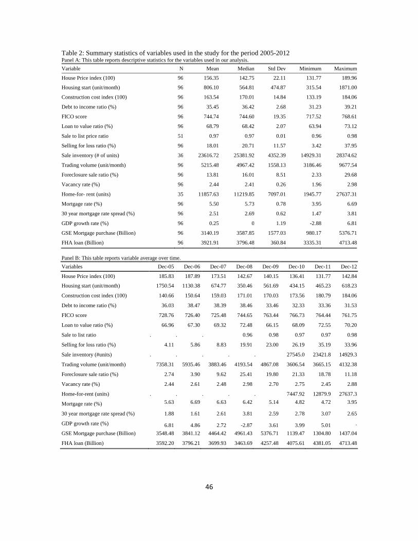
Table 2: Summary statistics of variables used in the study for the period 2005-2012 Panel A: This table reports descriptive statistics for the variables used in our analysis. Variable N Mean Median Std Dev Minimum Maximum
House Price index (100) 96 156.35 142.75 22.11 131.77 189.96
Housing start (unit/month) 96 806.10 564.81 474.87 315.54 1871.00
Construction cost index (100) 96 163.54 170.01 14.84 133.19 184.06
Debt to income ratio (%) 96 35.45 36.42 2.68 31.23 39.21
FICO score 96 744.74 744.60 19.35 717.52 768.61
Loan to value ratio (%) 96 68.79 68.42 2.07 63.94 73.12
Sale to list price ratio 51 0.97 0.97 0.01 0.96 0.98
Selling for loss ratio (%) 96 18.01 20.71 11.57 3.42 37.95
Sale inventory (# of units) 36 23616.72 25381.92 4352.39 14929.31 28374.62
Trading volume (unit/month) 96 5215.48 4967.42 1558.13 3186.46 9677.54
Foreclosure sale ratio (%) 96 13.81 16.01 8.51 2.33 29.68
Vacancy rate (%) 96 2.44 2.41 0.26 1.96 2.98
Home-for- rent (units) 35 11857.63 11219.85 7097.01 1945.77 27637.31
Mortgage rate (%) 96 5.50 5.73 0.78 3.95 6.69
30 year mortgage rate spread (%) 96 2.51 2.69 0.62 1.47 3.81
GDP growth rate (%) 96 0.25 0 1.19 -2.88 6.81
GSE Mortgage purchase (Billion) 96 3140.19 3587.85 1577.03 980.17 5376.71
FHA loan (Billion) 96 3921.91 3796.48 360.84 3335.31 4713.48 Panel B: This table reports variable average over time. Variables Dec-05 Dec-06 Dec-07 Dec-08 Dec-09 Dec-10 Dec-11 Dec-12
House Price index (100) 185.83 187.89 173.51 142.67 140.15 136.41 131.77 142.84
Housing start (unit/month) 1750.54 1130.38 674.77 350.46 561.69 434.15 465.23 618.23
Construction cost index (100) 140.66 150.64 159.03 171.01 170.03 173.56 180.79 184.06
Debt to income ratio (%) 36.03 38.47 38.39 38.46 33.46 32.33 33.36 31.53
FICO score 728.76 726.40 725.48 744.65 763.44 766.73 764.44 761.75
Loan to value ratio (%) 66.96 67.30 69.32 72.48 66.15 68.09 72.55 70.20
Sale to list ratio . . . 0.96 0.98 0.97 0.97 0.98
Selling for loss ratio (%) 4.11 5.86 8.83 19.91 23.00 26.19 35.19 33.96
Sale inventory (#units) . . . . . 27545.0 23421.8 14929.3
Trading volume (unit/month) 7358.31 5935.46 3883.46 4193.54 4867.08 3606.54 3665.15 4132.38
Foreclosure sale ratio (%) 2.74 3.90 9.62 25.41 19.80 21.33 18.78 11.18
Vacancy rate (%) 2.44 2.61 2.48 2.98 2.70 2.75 2.45 2.88
Home-for-rent (units) . . . . . 7447.92 12879.9 27637.3
Mortgage rate (%) 5.63 6.69 6.63 6.42 5.14 4.82 4.72 3.95
30 year mortgage rate spread (%) 1.88 1.61 2.61 3.81 2.59 2.78 3.07 2.65
GDP growth rate (%) 6.81 4.86 2.72 -2.87 3.61 3.99 5.01 .
GSE Mortgage purchase (Billion) 3548.48 3841.12 4464.42 4961.43 5376.71 1139.47 1304.80 1437.04
FHA loan (Billion) 3592.20 3796.21 3699.93 3463.69 4257.48 4075.61 4381.05 4713.48
46
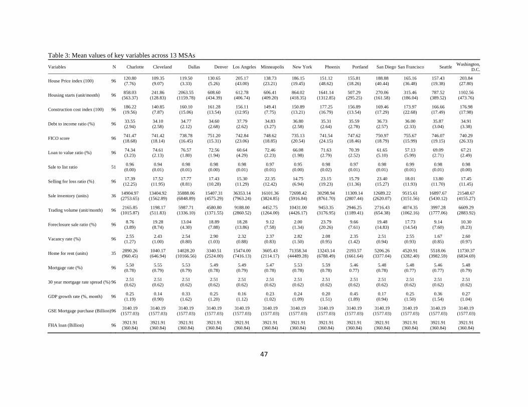
Table 3: Mean values of key variables across 13 MSAs
Variables N Charlotte Cleveland Dallas Denver Los Angeles Minneapolis New York Phoenix Portland San Diego San Francisco Seattle Washington, D.C.
House Price index (100) 96 120.80 (7.76)
109.35 (9.07)
119.50 (3.33)
130.65 (5.26)
205.17 (43.00)
138.73 (23.21)
186.15 (19.45)
151.12 (48.62)
155.81 (18.26)
188.88 (40.44)
165.16 (36.48)
157.43 (19.38)
203.84 (27.80)
Housing starts (unit/month) 96 858.03 (563.37)
241.86 (128.83)
2063.55 (1159.78)
608.60 (434.39)
612.78 (406.74)
606.41 (409.20)
864.02 (418.35)
1641.14 (1312.85)
507.29 (295.25)
270.06 (161.58)
315.46 (186.04)
787.52 (389.52)
1102.56 (473.76)
Construction cost index (100) 96 186.22 (19.56)
140.85 (7.87)
160.10 (15.06)
161.28 (13.54)
156.11 (12.95)
149.41 (7.75)
150.89 (13.21)
177.25 (16.79)
156.89 (13.54)
169.46 (17.29)
173.97 (22.68)
166.66 (17.49)
176.98 (17.98)
Debt to income ratio (%) 96 33.55 (2.94)
34.10 (2.58)
34.77 (2.12)
34.60 (2.68)
37.79 (2.62)
34.83 (3.27)
36.80 (2.58)
35.31 (2.64)
35.59 (2.78)
36.73 (2.57)
36.00 (2.33)
35.87 (3.04)
34.91 (3.38)
FICO score 96 741.47 (18.68)
741.42 (18.14)
738.78 (16.45)
751.20 (15.31)
742.84 (23.06)
748.62 (18.85)
735.13 (20.54)
741.54 (24.15)
747.62 (18.46)
750.97 (18.79)
755.67 (15.99)
746.07 (19.15)
740.29 (26.33)
Loan to value ratio (%) 96 74.34 (3.23)
74.61 (2.13)
76.57 (1.80)
72.56 (1.94)
60.64 (4.29)
72.46 (2.23)
66.08 (1.98)
71.63 (2.79)
70.39 (2.52)
61.65 (5.10)
57.13 (5.99)
69.09 (2.71)
67.21 (2.49)
Sale to list ratio 51 0.96 (0.00)
0.94 (0.01)
0.98 (0.01)
0.98 (0.00)
0.98 (0.01)
0.97 (0.01)
0.95 (0.00)
0.98 (0.02)
0.97 (0.01)
0.98 (0.01)
0.99 (0.01)
0.98 (0.01)
0.98 (0.00)
Selling for loss ratio (%) 96 17.39 (12.25)
17.52 (11.95)
17.77 (8.81)
17.43 (10.28)
15.30 (11.29)
22.35 (12.42)
14.75 (6.94)
23.15 (19.23)
15.79 (11.36)
23.40 (15.27)
18.01 (11.93)
13.80 (11.70)
17.45 (11.45)
Sale inventory (units) 36 14904.97 (2753.65)
13404.92 (1562.89)
35888.06 (6848.89)
15407.31 (4575.29)
36353.14 (7963.24)
16101.36 (3824.85)
72698.42 (5916.84)
30298.94 (8761.70)
11309.14 (2807.44)
12689.22 (2620.07)
9515.61 (3151.56)
16897.67 (5430.12)
21548.67 (4155.27)
Trading volume (unit/month) 96 2165.85 (1015.87)
1198.17 (511.83)
5987.71 (1336.10)
4580.80 (1371.55)
9188.00 (2860.52)
4452.75 (1264.00)
10431.00 (4426.17)
9453.35 (3176.95)
2946.25 (1189.41)
2716.43 (654.38)
4074.35 (1062.16)
3997.28 (1777.06)
6609.29 (2883.92)
Foreclosure sale ratio (%) 96 8.76 (3.89)
19.28 (8.74)
13.04 (4.30)
18.89 (7.88)
18.28 (13.86)
9.12 (7.58)
2.00 (1.34)
23.79 (20.26)
9.66 (7.61)
19.48 (14.83)
17.73 (14.54)
9.14 (7.60)
10.30 (8.23)
Vacancy rate (%) 96 2.55 (1.27)
2.43 (1.00)
2.54 (0.80)
2.90 (1.03)
2.32 (0.88)
2.37 (0.83)
2.82 (1.50)
2.08 (0.95)
2.35 (1.42)
2.51 (0.94)
2.55 (0.93)
1.67 (0.85)
2.60 (0.97)
Home for rent (units) 35 2890.26 (960.45)
1040.17 (646.94)
14028.20 (10166.56)
3340.51 (2524.00)
15474.00 (7416.13)
3605.43 (2114.17)
71358.34 (44489.28)
13243.14 (6788.49)
2193.57 (1661.64)
5206.26 (3377.04)
4520.91 (3282.40)
5518.06 (3982.59)
11730.37 (6834.69)
Mortgage rate (%) 96 5.50 (0.78)
5.55 (0.79)
5.53 (0.79)
5.49 (0.78)
5.49 (0.79)
5.47 (0.78)
5.53 (0.78)
5.59 (0.78)
5.46 0.77)
5.48 (0.78)
5.48 (0.77)
5.46 (0.77)
5.48 (0.79)
30 year mortgage rate spread (%) 96 2.51 (0.62)
2.51 (0.62)
2.51 (0.62)
2.51 (0.62)
2.51 (0.62)
2.51 (0.62)
2.51 (0.62)
2.51 (0.62)
2.51 (0.62)
2.51 (0.62)
2.51 (0.62)
2.51 (0.62)
2.51 (0.62)
GDP growth rate (%, month) 96 0.25 (1.19)
0.14 (0.90)
0.33 (1.62)
0.25 (1.20)
0.16 (1.12)
0.23 (1.02)
0.24 (1.09)
0.20 (1.51)
0.45 (1.89)
0.17 (0.94)
0.25 (1.50)
0.36 (1.54)
0.27 (1.04)
GSE Mortgage purchase (Billion) 96 3140.19 (1577.03)
3140.19 (1577.03)
3140.19 (1577.03)
3140.19 (1577.03)
3140.19 (1577.03)
3140.19 (1577.03)
3140.19 (1577.03)
3140.19 (1577.03)
3140.19 (1577.03)
3140.19 (1577.03)
3140.19 (1577.03)
3140.19 (1577.03)
3140.19 (1577.03)
FHA loan (Billion) 96 3921.91 (360.84)
3921.91 (360.84)
3921.91 (360.84)
3921.91 (360.84)
3921.91 (360.84)
3921.91 (360.84)
3921.91 (360.84)
3921.91 (360.84)
3921.91 (360.84)
3921.91 (360.84)
3921.91 (360.84)
3921.91 (360.84)
3921.91 (360.84)
47

Table 4: Percentage change of variables at different time intervals
%change from
2005:01-2008:09 % change from
2008:09-2012:12 % change from
2005:01-2012:12 House Price index -7.99 -5.31 -12.87
Housing start -69.04 24.82 -61.36
Construction cost index 26.21 8.93 37.47
Debt to income ratio 3.09 -17.13 -14.57
FICO score 3.23 2.85 6.17
Loan to value ratio 0.61 0.32 0.94
Sale to list ratio 2.11
Sale for loss ratio 279.89 116.49 722.41
Sale inventory -37.95 Trading volume -16.68 -24.87 -37.40
Foreclosure sale ratio 559.11 -43.88 269.91
Vacancy rate 16.79 16.88 36.50
Home-for- rent 1320.38
Mortgage rate -1.65 -33.67 -34.76
30 year mortgage rate spread 58 -16.14 32.5
GSE Mortgage purchase 43.60 -70.63 -57.82
FHA loan -10.07 41.32 27.09
Note: Sale to list ratio is available from 2008:10 to 2012:12. Sale inventory is available from 2010:01 to 2012:12. Home-for-rent is available from 2010:02 to 2012:12.
48

Table 5: Pair-wise correlation matrix of variables
Price index (100)
Housing start
(unit/month)
Construction cost
index (100)
Debt to income
ratio (%)
FICO score
Loan to value ratio (%)
Sale to list ratio
(X)
Selling for loss
ratio (%)
Sale inventory (units)
Trading volume (unit/mo
nth)
Foreclosure sale
ratio (%)
Vacancy rate (%)
Home for rent (units)
Mortgage rate (%)
30 year mortgag
e rate spread
(%)
GDP growth rate (%)
GSE Mortgag
e purchase (Billion)
FHA loan
(Billion)
Price index (100) 1.000 0.184 -0.278 0.595 -0.501 -0.681 0.223 -0.542 0.318 0.483 -0.513 0.010 0.323 0.386 -0.439 0.040 0.243 -0.359
Housing start 0.184 1.000 -0.310 0.190 -0.544 0.247 0.308 -0.441 0.299 0.501 -0.414 -0.030 0.220 0.271 -0.511 0.077 0.137 -0.325
Construction cost index (100)
-0.278 -0.310 1.000 -0.462 0.633 0.029 0.433 0.668 -0.245 -0.259 0.469 0.014 -0.057 -0.493 0.600 -0.030 -0.319 0.553
Debt to income ratio (%)
0.595 0.190 -0.462 1.000 -0.760 -0.223 -0.139 -0.689 0.340 0.312 -0.295 -0.022 0.127 0.865 -0.315 -0.026 0.599 -0.727
FICO score -0.501 -0.544 0.633 -0.760 1.000 -0.051 0.516 0.852 -0.464 -0.384 0.594 0.023 -0.333 -0.812 0.607 -0.008 -0.552 0.742
Loan to value ratio -0.681 0.247 0.029 -0.223 -0.051 1.000 -0.273 0.158 -0.139 -0.199 0.091 0.007 -0.112 -0.001 0.189 -0.019 -0.065 0.069
Sale to list ratio (X)
0.223 0.308 0.433 -0.139 0.516 -0.273 1.000 0.369 -0.328 0.315 0.159 -0.098 -0.220 -0.348 -0.270 0.019 -0.180 0.330
Selling for loss ratio (%)
-0.542 -0.441 0.668 -0.689 0.852 0.158 0.369 1.000 -0.321 -0.282 0.642 0.023 -0.132 -0.761 0.677 -0.020 -0.565 0.778
Sale inventory 0.318 0.299 -0.245 0.340 -0.464 -0.139 -0.328 -0.321 1.000 0.628 -0.227 0.070 0.665 0.215 0.005 0.003 -0.177 -0.205
Trading volume 0.483 0.501 -0.259 0.312 -0.384 -0.199 0.315 -0.282 0.628 1.000 -0.214 -0.076 0.419 0.171 -0.318 -0.031 0.131 -0.238
Foreclosure sale ratio (%)
-0.513 -0.414 0.469 -0.295 0.594 0.091 0.159 0.642 -0.227 -0.214 1.000 -0.027 -0.440 -0.285 0.595 -0.078 -0.127 0.281
Vacancy rate (%) 0.010 -0.030 0.014 -0.022 0.023 0.007 -0.098 0.023 0.070 -0.076 -0.027 1.000 -0.010 -0.025 0.041 0.033 -0.008 0.028
Home for rent 0.323 0.220 -0.057 0.127 -0.333 -0.112 -0.220 -0.132 0.665 0.419 -0.440 -0.010 1.000 -0.271 0.056 -0.017 0.300 0.283
Mortgage rate (%) 0.386 0.271 -0.493 0.865 -0.812 -0.001 -0.348 -0.761 0.215 0.171 -0.285 -0.025 -0.271 1.000 -0.388 -0.016 0.716 -0.823
30 year mortgage rate spread (%)
-0.439 -0.511 0.600 -0.315 0.607 0.189 -0.270 0.677 0.005 -0.318 0.595 0.041 0.056 -0.388 1.000 -0.105 -0.175 0.378
GDP growth rate (%)
0.040 0.077 -0.030 -0.026 -0.008 -0.019 0.019 -0.020 0.003 -0.031 -0.078 0.033 -0.017 -0.016 -0.105 1.000 -0.096 0.003
GSE Mortgage purchase (Billion)
0.243 0.137 -0.319 0.599 -0.552 -0.065 -0.180 -0.565 -0.177 0.131 -0.127 -0.008 0.300 0.716 -0.175 -0.096 1.000 -0.703
FHA loan (Billion) -0.359 -0.325 0.553 -0.727 0.742 0.069 0.330 0.778 -0.205 -0.238 0.281 0.028 0.283 -0.823 0.378 0.003 -0.703 1.000
49

Table 6: Results of Principal component analysis . Panel A: Eigenvalue in the principal component analysis. Eigenvalue Difference Cumulative
Eigenvalue Proportion Cumulative
Proportion 1 2.7180 0.8733 2.7180 0.2091 0.2091
2 1.8446 0.4055 4.5626 0.1419 0.3510
3 1.4391 0.4145 6.0017 0.1107 0.4617
4 1.0247 0.0492 7.0264 0.0788 0.5405
5 0.9755 0.0076 8.0019 0.0750 0.6155
6 0.9678 0.1188 8.9697 0.0744 0.6900
7 0.8490 0.1355 9.8187 0.0653 0.7553
8 0.7135 0.1005 10.5322 0.0549 0.8102
9 0.6130 0.0583 11.1452 0.0472 0.8573
10 0.5547 0.0386 11.6999 0.0427 0.9000
11 0.5161 0.0770 12.2160 0.0397 0.9397
12 0.4391 0.0941 12.6551 0.0338 0.9735
13 0.3449 13 0.0265 1
Panel B Standardized scoring coefficients (Factor Loadings)
Factor1 Factor2 Factor3 Factor4 Growth rate of Debt to income ratio 0.3404 * -0.0591 -0.0158 -0.0453
Growth rate of FICO score -0.3033 * 0.0840 -0.0452 0.0529
Growth rate of Loan to value ratio 0.2941 * 0.0086 0.0177 0.0643
Growth rate of mortgage rate 0.3333 * 0.0069 0.0315 -0.0350
Growth rate of Sale to list ratio -0.0253 -0.1799 * 0.0182 -0.3492 *
Growth rate of Selling for loss ratio -0.0214 0.3543 * 0.0349 -0.1791
Growth rate of Trading volume 0.0189 -0.4127 * -0.0156 -0.0692
Growth rate of Foreclosure sale ratio -0.0379 0.4169 * -0.0120 -0.0134
Growth rate of GSE mortgage purchase -0.0249 0.0726 0.5310 * -0.0001
Growth rate of FHA loan 0.0642 0.0264 0.2790 * 0.1582
Growth rate of Sale inventory -0.0039 -0.0360 -0.5049 * 0.0750
Growth rate of Home for rent -0.0512 -0.1217 0.0655 0.8671 *
Growth rate of Vacancy rate -0.0385 0.2019 0.0969 -0.0496
Note: Factor1 is Aggregate Funding liquidity Factor; Factor2 is Market illiquidity Factor; Factor3 is Credit Availability Liquidity Factor (liquidity induced by QE via GSE and FHA credit activities), and Factor4 is Shadow vacancy Liquidity Factor (inventory of home-for-rent)
50
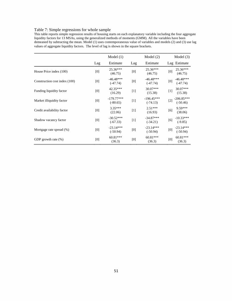
Table 7: Simple regressions for whole sample This table reports simple regression results of housing starts on each explanatory variable including the four aggregate liquidity factors for 13 MSAs, using the generalized methods of moments (GMM). All the variables have been demeaned by subtracting the mean. Model (1) uses contemporaneous value of variables and models (2) and (3) use lag values of aggregate liquidity factors. The level of lag is shown in the square brackets.
Model (1) Model (2) Model (3)
Lag Estimate Lag Estimate Lag Estimate
House Price index (100) [0] 25.36*** (46.75) [0] 25.36***
(46.75) [0] 25.36*** (46.75)
Construction cost index (100) [0] -46.48*** (-47.74) [0] -46.48***
(-47.74) [0] -46.48*** (-47.74)
Funding liquidity factor [0] 42.35*** (16.29) [1] 30.07***
(15.38) [1] 30.07*** (15.38)
Market illiquidity factor [0] -179.77*** (-80.65) [1] -196.45***
(-74.13) [2] -206.85*** (-50.46)
Credit availability factor [0] 3.35*** (22.06) [1] 2.51***
(16.93) [6] 9.59*** (38.06)
Shadow vacancy factor [0] -30.52*** (-67.33) [1] -34.87***
(-34.21) [6] -10.33*** (-9.85)
Mortgage rate spread (%) [0] -23.14*** (-50.94) [0] -23.14***
(-50.94) [0] -23.14*** (-50.94)
GDP growth rate (%) [0] 60.81*** (36.3) [0] 60.81***
(36.3) [0] 60.81*** (36.3)
51

Table 8: Multivariate panel regression of housing starts This table reports multivariate regression results for the whole sample. The procedure used is GMM with panel data techniques, that is pooled fixed effects model. All series have been de-trended by subtracting the cross-sectional means to mitigate the of cross-sectional dependence. The regressions are estimated for both the structural model and reduced form model. The first three column show the regression based on contemporaneous value of explanatory variables and the last three columns show results with liquidity factor, market illiquidity factor, credit availability factor and shadow vacancy factor lagged at 1, 2, 6, and 6 months, respectively.
No lag With lag
Structural
Model Reduced
Form model Reduced
form model with interaction
Structural Model
Reduced Form Model
Reduced form model
with interaction Housing price index (100) 3.77***
(5.61) 3.42*** (5.21)
Construction cost index (100) -46.85*** (-60.84)
-49.03*** (-86.37)
-48.98*** (-86.32)
-47.06*** (-61.06)
-49.33*** (-85.67)
-49.09*** (-85.41)
Funding liquidity actor 22.87***
(2.71) 15.07* (1.73) 22.48***
(2.66) 13.23 (1.54)
Market illiquidity factor -43.96*** (-4.81)
-55.39*** (-6.31)
-45.24*** (-4.9)
-80.99*** (-9.13)
-76.17*** (-9.09)
-72.33*** (-8.64)
Funding liquidity*market illiquidity
-40.39*** (-3.56) -59.49***
(-5.67)
Credit availability factor 32.03*** (4.37)
55.35*** (7.6)
53.9*** (7.4)
56.19*** (7.08)
56.34*** (7.34)
54.36*** (7.11)
Shadow vacancy factor -21.35*** (-2.61)
-16.9** (-2.17)
-10.87 (-1.36)
-42.05*** (-4.03)
-43.26*** (-4.27)
-50.21*** (-4.94)
Mortgage rate spread (%) -8.07*** (-5.57)
-5.84*** (-4.23)
-6.17*** (-4.46)
-9.71*** (-6.75)
-8.03*** (-5.86)
-8.3*** (-6.08)
GDP growth rate (%) 55.22***
(8.86) 52.55***
(8.37) 31.63*** (5.6)
30.66*** (5.45)
52
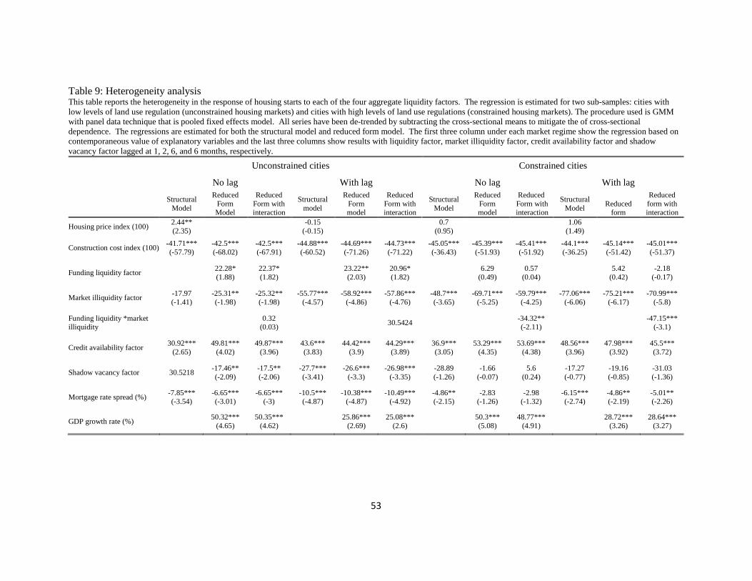
Table 9: Heterogeneity analysis This table reports the heterogeneity in the response of housing starts to each of the four aggregate liquidity factors. The regression is estimated for two sub-samples: cities with low levels of land use regulation (unconstrained housing markets) and cities with high levels of land use regulations (constrained housing markets). The procedure used is GMM with panel data technique that is pooled fixed effects model. All series have been de-trended by subtracting the cross-sectional means to mitigate the of cross-sectional dependence. The regressions are estimated for both the structural model and reduced form model. The first three column under each market regime show the regression based on contemporaneous value of explanatory variables and the last three columns show results with liquidity factor, market illiquidity factor, credit availability factor and shadow vacancy factor lagged at 1, 2, 6, and 6 months, respectively.
Unconstrained cities Constrained cities
No lag With lag No lag With lag
Structural
Model
Reduced Form Model
Reduced Form with interaction
Structural model
Reduced Form model
Reduced Form with interaction
Structural Model
Reduced Form model
Reduced Form with interaction
Structural Model
Reduced
form
Reduced form with interaction
Housing price index (100) 2.44** (2.35) -0.15
(-0.15) 0.7 (0.95)
1.06 (1.49)
Construction cost index (100) -41.71*** (-57.79)
-42.5*** (-68.02)
-42.5*** (-67.91)
-44.88*** (-60.52)
-44.69*** (-71.26)
-44.73*** (-71.22)
-45.05*** (-36.43)
-45.39*** (-51.93)
-45.41*** (-51.92)
-44.1*** (-36.25)
-45.14*** (-51.42)
-45.01*** (-51.37)
Funding liquidity factor 22.28* (1.88)
22.37* (1.82) 23.22**
(2.03) 20.96* (1.82)
6.29 (0.49)
0.57 (0.04)
5.42 (0.42)
-2.18 (-0.17)
Market illiquidity factor -17.97 (-1.41)
-25.31** (-1.98)
-25.32** (-1.98)
-55.77*** (-4.57)
-58.92*** (-4.86)
-57.86*** (-4.76)
-48.7*** (-3.65)
-69.71*** (-5.25)
-59.79*** (-4.25)
-77.06*** (-6.06)
-75.21*** (-6.17)
-70.99*** (-5.8)
Funding liquidity *market illiquidity 0.32
(0.03) 30.5424 -34.32** (-2.11)
-47.15*** (-3.1)
Credit availability factor 30.92*** (2.65)
49.81*** (4.02)
49.87*** (3.96)
43.6*** (3.83)
44.42*** (3.9)
44.29*** (3.89)
36.9*** (3.05)
53.29*** (4.35)
53.69*** (4.38)
48.56*** (3.96)
47.98*** (3.92)
45.5*** (3.72)
Shadow vacancy factor 30.5218 -17.46** (-2.09)
-17.5** (-2.06)
-27.7*** (-3.41)
-26.6*** (-3.3)
-26.98*** (-3.35)
-28.89 (-1.26)
-1.66 (-0.07)
5.6 (0.24)
-17.27 (-0.77)
-19.16 (-0.85)
-31.03 (-1.36)
Mortgage rate spread (%) -7.85*** (-3.54)
-6.65*** (-3.01)
-6.65*** (-3)
-10.5*** (-4.87)
-10.38*** (-4.87)
-10.49*** (-4.92)
-4.86** (-2.15)
-2.83 (-1.26)
-2.98 (-1.32)
-6.15*** (-2.74)
-4.86** (-2.19)
-5.01** (-2.26)
GDP growth rate (%) 50.32*** (4.65)
50.35*** (4.62) 25.86***
(2.69) 25.08***
(2.6) 50.3*** (5.08)
48.77*** (4.91)
28.72*** (3.26)
28.64*** (3.27)
53
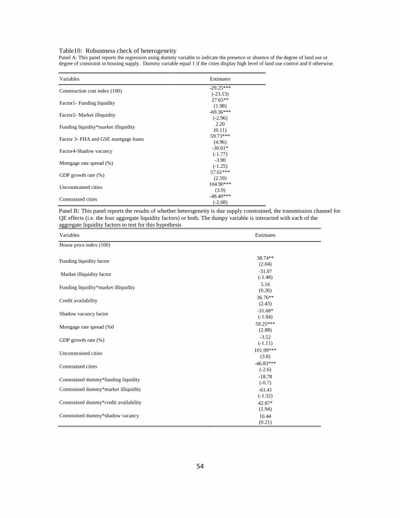
Table10: Robustness check of heterogeneity Panel A: This panel reports the regression using dummy variable to indicate the presence or absence of the degree of land use or degree of constraint in housing supply. Dummy variable equal 1 if the cities display high level of land use control and 0 otherwise.
Variables Estimates
Construction cost index (100) -29.25*** (-23.13)
Factor1- Funding liquidity 27.65** (1.98)
Factor2- Market illiquidity -69.36*** (-2.96)
Funding liquidity*market illiquidity 2.20 (0.11)
Factor 3- FHA and GSE mortgage loans 59.73*** (4.96)
Factor4-Shadow vacancy -30.61* (-1.77)
Mortgage rate spread (%) -3.90 (-1.25)
GDP growth rate (%) 57.61*** (2.59)
Unconstrained cities 104.90*** (3.9)
Constrained cities -48.40*** (-2.68)
Panel B: This panel reports the results of whether heterogeneity is due supply constrained, the transmission channel for QE effects (i.e. the four aggregate liquidity factors) or both. The dumpy variable is interacted with each of the aggregate liquidity factors to test for this hypothesis
Variables Estimates
House price index (100)
Funding liquidity factor 38.74**
(2.04)
Market illiquidity factor -31.07 (-1.48)
Funding liquidity*market illiquidity 5.16 (0.26)
Credit availability 36.76** (2.43)
Shadow vacancy factor -31.68* (-1.84)
Mortgage rate spread (%0 59.25*** (2.88)
GDP growth rate (%) -3.52 (-1.11)
Unconstrained cities 101.99*** (3.8)
Constrained cities -46.83*** (-2.6)
Constrained dummy*funding liquidity -18.78 (-0.7)
Constrained dummy*market illiquidity -61.41 (-1.32)
Constrained dummy*credit availability 42.87* (1.94)
Constrained dummy*shadow vacancy 16.44 (0.21)
54

Table 11 Changes in housing start changes due to shocks to major policy variables and the aggregate liquidity factors Panel A: Effect of change in LTV on housing starts
Date LTV level Housing start Compound annual growth rate
13-city average LTV for low down-payment loans 68.79% 1053.16 New LTV due to change +4.60% 73.39% 1067.53 17.66% Panel B: Effect of change in debt-to-income (DTI) on housing starts
Date DTI level Housing start Compound annual growth rate
13-city average DTI over sample period 35.45% 1053.16 New DTI due to change of +6.55% 42% 1164.43 233.76% Panel C: Effect of change in FICO score on housing starts
Date FICO level Housing start Compound annual growth rate
13-city average FICO score over sample period 744.74 1053.16 New average FICO score due to change of +35.6 780.00 922.41 -79.62% Panel D Effect of change in GSE mortgage purchase on housing start
Date GSE mortgage level Housing start Compound annual
growth rate 13-city average over sample period 3140.19 1053.16 New purchase level due to change of $359.81B 3500.00 1082.56 39.15% Panel E Effect of change in FHA loan on housing start
Date FHA loan level Housing start Compound annual growth rate
13-city average over sample period 3921.91 1053.16 New purchase level due change of +$4278.09B 4200.00 1087.27 46.59% Panel E Effect of change in rate spread by 150 bps on housing start
Date Rate spread Housing start Compound annual growth rate
13-city average mortgage spread over sample period 2.51% 1053.16 New spread due to change of +150 bps 4.01% 1049.51 -4.08% Panel F Effect of change in factor on housing start Change one standard deviation in Factors
Expected housing start after
Expected housing start before
Compound annual growth rate
Funding liquidity (add one σ) 1067.60 1053.16 17.75%
Market illiquidity (minus one σ) 1098.84 1053.16 66.45%
Credit availability (add one σ) 1107.06 1053.16 82.02%
Shadow vacancy (minus one σ) 1064.03 1053.16 13.11%
55
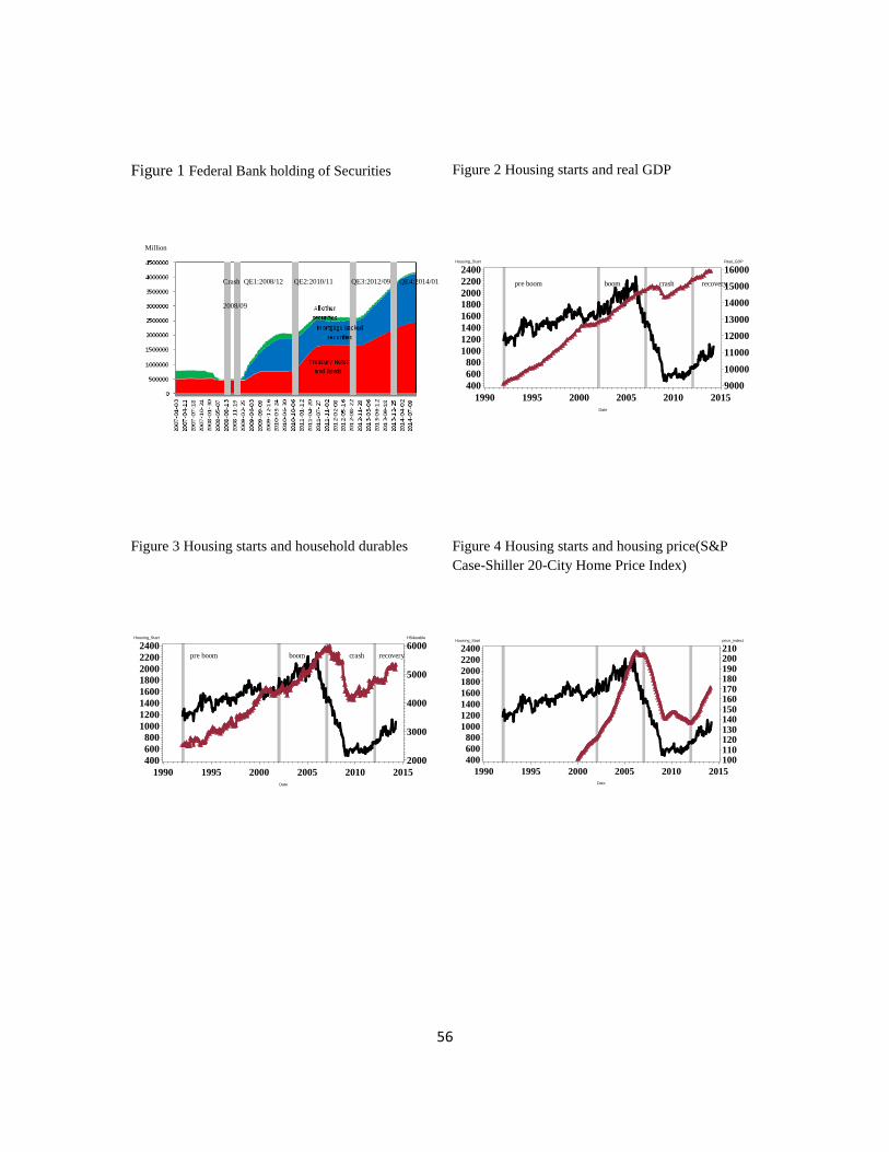
Figure 1 Federal Bank holding of Securities
Figure 2 Housing starts and real GDP
Housing_Start
400600800
10001200140016001800200022002400
Date
1990 1995 2000 2005 2010 2015
Real_GDP
900010000
11000
1200013000
14000
1500016000
Figure 3 Housing starts and household durables
Housing_Start
400600800
10001200140016001800200022002400
Date
1990 1995 2000 2005 2010 2015
HSdurable
2000
3000
4000
5000
6000
Figure 4 Housing starts and housing price(S&P Case-Shiller 20-City Home Price Index)
Housing_Start
400600800
10001200140016001800200022002400
Date
1990 1995 2000 2005 2010 2015
price_indext
100110120130140150160170180190200210
Crash QE1:2008/12 QE2:2010/11 QE3:2012/09 QE4:2014/01
2008/09
Million
pre boom boom crash recovery
pre boom boom crash recovery
56

Figure 5: Cumulative level of funding liquidity and the time series of three key variables (debt to income ratio, FICO score, and LTV) that load on funding liquidity. Panel A: Funding liquidity, debt to income ratio, FICO score, and LTV
Variables
-5
-4
-3
-2
-1
0
1
2
3
4
Date
01JAN2005 01JAN2006 01JAN2007 01JAN2008 01JAN2009 01JAN2010 01JAN2011 01JAN2012 01JAN2013
Funding Liquidity
-0.06
-0.05
-0.04
-0.03
-0.02
-0.01
0.00
0.01
0.02
0.03
0.04
0.05
0.06
Debt to income ratio FICO score Loan to value ratio
Funding liquidity
Panel B Funding liquidity, debt to income ratio, and FICO score
Panel C Funding liquidity, loan to value ratio, and FICO score
Panel D Funding liquidity, loan to value ratio, and debt to income ratio
Panel E Funding liquidity, FICO score, and mortgage rate
57

Figure 6: Cumulative level of market illiquidity and the time series of four key variables (sale to list ratio, selling for loss ratio, trading volume, and foreclosure sale ratio) that load on the market illiquidity factor. Panel A: Market illiquidity, sale to list ratio, selling for loss ratio, trading volume, and foreclosure sale ratio
Variables
-8-7-6-5-4-3-2-101234567
Date
01JAN2005 01JAN2006 01JAN2007 01JAN2008 01JAN2009 01JAN2010 01JAN2011 01JAN2012 01JAN2013
Market Illiquidity
-0.05-0.04-0.03-0.02-0.010.000.010.020.030.040.050.060.070.080.090.100.110.120.130.14
Sale to list ratio Selling for loss ratio Trading volume Foreclosure sale ratio
Market illiquidity
58

Panel B Market illiquidity, sale to list ratio, and foreclosure sale ratio
Panel C Market illiquidity, sale to list ratio, and selling for loss ratio
Panel D Market illiquidity, trading volume, and selling for loss ratio
Panel E Market illiquidity, sale to list ratio, and trading volume
Panel F Market illiquidity, trading volume, and foreclosure sale ratio
Panel G Market illiquidity, foreclosure sale ratio, and selling for loss ratio
59
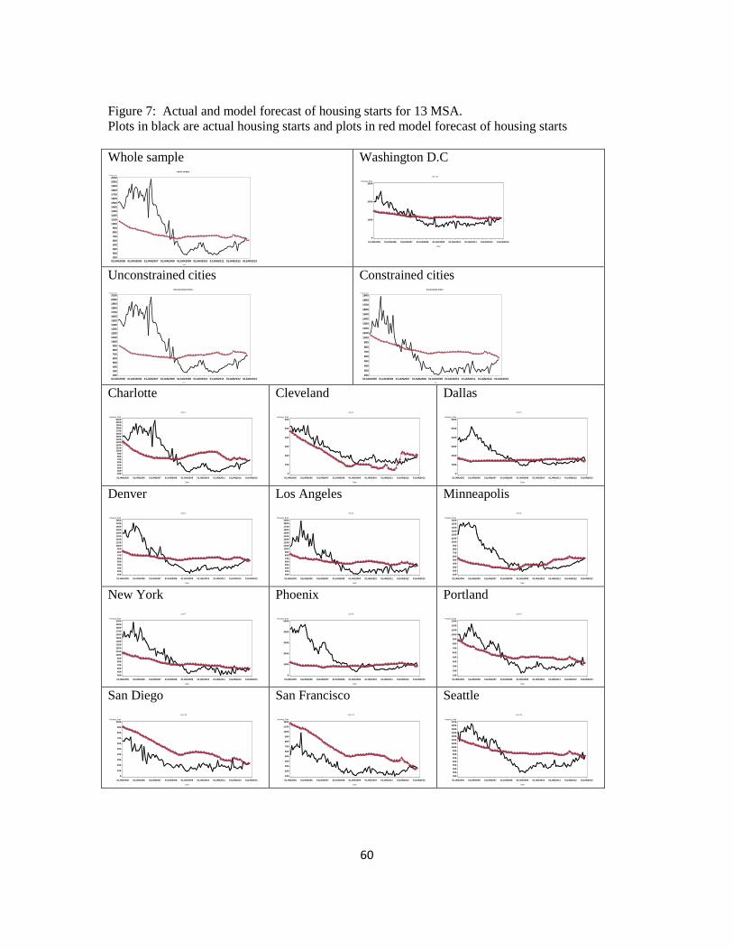
Figure 7: Actual and model forecast of housing starts for 13 MSA. Plots in black are actual housing starts and plots in red model forecast of housing starts Whole sample
Housing_Start
200300400500600700800900
100011001200130014001500160017001800190020002100
Date
01JAN2005 01JAN2006 01JAN2007 01JAN2008 01JAN2009 01JAN2010 01JAN2011 01JAN2012 01JAN2013
whole sample
Washington D.C Housing_Start
0
1000
2000
3000
Date
01JAN2005 01JAN2006 01JAN2007 01JAN2008 01JAN2009 01JAN2010 01JAN2011 01JAN2012 01JAN2013
city=13
Unconstrained cities Housing_Start
200300400500600700800900
100011001200130014001500160017001800190020002100
Date
01JAN2005 01JAN2006 01JAN2007 01JAN2008 01JAN2009 01JAN2010 01JAN2011 01JAN2012 01JAN2013
Unconstrained Cities
Constrained cities Housing_Start
200300400
500600700800
900100011001200
1300140015001600
170018001900
Date
01JAN2005 01JAN2006 01JAN2007 01JAN2008 01JAN2009 01JAN2010 01JAN2011 01JAN2012 01JAN2013
Constrained Cities
Charlotte
Housing_Start
200300400500600700800900
100011001200130014001500160017001800190020002100
Date
01JAN2005 01JAN2006 01JAN2007 01JAN2008 01JAN2009 01JAN2010 01JAN2011 01JAN2012 01JAN2013
city=1
Cleveland Housing_Start
0
100
200
300
400
500
600
Date
01JAN2005 01JAN2006 01JAN2007 01JAN2008 01JAN2009 01JAN2010 01JAN2011 01JAN2012 01JAN2013
city=2
Dallas Housing_Start
0
1000
2000
3000
4000
5000
6000
Date
01JAN2005 01JAN2006 01JAN2007 01JAN2008 01JAN2009 01JAN2010 01JAN2011 01JAN2012 01JAN2013
city=3
Denver
Housing_Start
100200300400500600700800900
100011001200130014001500160017001800
Date
01JAN2005 01JAN2006 01JAN2007 01JAN2008 01JAN2009 01JAN2010 01JAN2011 01JAN2012 01JAN2013
city=4
Los Angeles Housing_Start
200300400500600700800900
1000110012001300140015001600170018001900
Date
01JAN2005 01JAN2006 01JAN2007 01JAN2008 01JAN2009 01JAN2010 01JAN2011 01JAN2012 01JAN2013
city=5
Minneapolis Housing_Start
100200300400500600700800900
1000110012001300140015001600
Date
01JAN2005 01JAN2006 01JAN2007 01JAN2008 01JAN2009 01JAN2010 01JAN2011 01JAN2012 01JAN2013
city=6
New York
Housing_Start
400500600700800900
10001100120013001400150016001700180019002000
Date
01JAN2005 01JAN2006 01JAN2007 01JAN2008 01JAN2009 01JAN2010 01JAN2011 01JAN2012 01JAN2013
city=7
Phoenix Housing_Start
0
1000
2000
3000
4000
5000
Date
01JAN2005 01JAN2006 01JAN2007 01JAN2008 01JAN2009 01JAN2010 01JAN2011 01JAN2012 01JAN2013
city=8
Portland Housing_Start
100
200
300
400
500
600
700
800
900
1000
1100
1200
1300
Date
01JAN2005 01JAN2006 01JAN2007 01JAN2008 01JAN2009 01JAN2010 01JAN2011 01JAN2012 01JAN2013
city=9
San Diego
Housing_Start
0
100
200
300
400
500
600
700
800
900
1000
Date
01JAN2005 01JAN2006 01JAN2007 01JAN2008 01JAN2009 01JAN2010 01JAN2011 01JAN2012 01JAN2013
city=10
San Francisco Housing_Start
100
200
300
400
500
600
700
800
900
1000
1100
1200
Date
01JAN2005 01JAN2006 01JAN2007 01JAN2008 01JAN2009 01JAN2010 01JAN2011 01JAN2012 01JAN2013
city=11
Seattle Housing_Start
200300400500600700800900
10001100120013001400150016001700
Date
01JAN2005 01JAN2006 01JAN2007 01JAN2008 01JAN2009 01JAN2010 01JAN2011 01JAN2012 01JAN2013
city=12
60

Figure 8: Plots of housing starts from counterfactual analysis. Housing starts plots in black are for the policy scenario (i.e. the Fed intervenes via QE) that reflects the stimulus effects of QE, and plots in red are the no policy scenario (i.e. the Fed does not intervene via QE) that does not reflect the stimulus effects of QE. For the no policy scenario the model is calibrated by fixing the aggregate liquidity factors at events dates prior to initiation of QE and after the initiation of QE. 2007/08-2012/12 9 (BNP Paribus terminated withdrawal from three of its hedge funds Starts average With QE 698.78 Without QE 389.58
Housing_Start
-1000
100200300400500600700800
Date
01JAN2006 01JAN2008 01JAN2010 01JAN2012 01JAN2014
2008/09-2012/12 (Leman Brother files for bankruptcy) Starts average With QE 701.02 Without QE 565.28
Housing_Start
100
200
300
400
500
600
700
800
Date
01JAN2008 01JAN2009 01JAN2010 01JAN2011 01JAN2012 01JAN2013
2008/12-2012/12 (initiation of QE1) Starts average With QE 702.91 Without QE 571.75
Housing_Start
100
200
300
400
500
600
700
800
Date
01JAN2008 01JAN2009 01JAN2010 01JAN2011 01JAN2012 01JAN2013
2010/11-2012/12 (Q1, QE2 in place and QE3 announced) Starts average With QE 694.21 Without QE 658.76
Housing_Start
300
400
500
600
700
800
Date
01JUL2010 01JAN2011 01JUL2011 01JAN2012 01JUL2012 01JAN2013
61


