DISSERTATION
Numerical Simulations of Metal Matrix Composites -
Tribological Behavior and Finite Strain Response on
Different Length Scales
ausgefuhrt zum Zwecke der Erlangung des akademischen Grades eines
Doktors der technischen Wissenschaften unter der Leitung von
Univ.Doz. Dipl.-Ing. Dr.techn. Heinz Pettermann
E317
Institut fur Leichtbau und Struktur–Biomechanik
eingereicht an der Technischen Universitat Wien
Fakultat fur Maschinenwesen und Betriebswissenschaften
von
Dipl.-Ing. Christopher O. HUBER
Matrikelnummer: 9125447
Pannaschg. 7/2/5
1050 Wien
Wien, im Februar 2008 Christopher Huber
Die approbierte Originalversion dieser Dissertation ist an der Hauptbibliothek der Technischen Universität Wien aufgestellt (http://www.ub.tuwien.ac.at). The approved original version of this thesis is available at the main library of the Vienna University of Technology (http://www.ub.tuwien.ac.at/englweb/).

III
ABSTRACT
The present thesis is concerned with the computational simulation of Metal Matrix Com-
posites (MMCs), a material where particulate reinforcements are embedded in a metal
phase, and which bears the potential to be tailored to particular applications. The ob-
jective of this work is to improve computational predictions, on the one hand, of the
thermo-mechanical behavior in frictional contact and, on the other hand, of the elasto-
plastic properties of MMCs undergoing finite strains. Both topics follow a hierarchical
approach employing micromechanical methods within the continuum mechanics approach.
The first executive chapter deals with computational predictions of the tribological be-
havior of MMCs. The influence of particle volume fraction and clustering of particles is
investigated at different length scales. Finite Element simulations are performed employ-
ing periodic unit cells based on homogeneous, randomly distributed inclusions in a matrix
phase with 30% particle volume fraction. In addition, the present work introduces mod-
ified unit cells with 10% particle volume fraction, with both homogeneous random and
clustered distributions. These modifications are derived from the original cell by either
randomly removing inclusions in the former case, or from a predefined area in the latter
case. Based on these experiences, numerical simulations employing the Finite Element
Method (FEM) of the frictional behavior of a MMC material, including heat conduction
in the steady state, are performed. Experiments and analytical calculations serve to de-
termine certain unknown process parameters by employing a simplified model by means of
homogenizing the material. Within the scope of this model, heat transfer and conduction
ABSTRACT
are described. In the FEM simulations, the inhomogeneous body is considered. Limitations
of the thermo-elastic FEM predictions are related to frictionally excited thermo-elastic in-
stability, the stability limit is estimated analytically using two different approaches from
the literature and compared to the simulation findings. The limited number of experi-
mental tests does not allow for quantitatively reliable results but the analytical and the
FEM simulations’ predictions are qualitatively compared. The practical consequences of
thermoelastic instability are discussed.
The second executive chapter deals with computational simulations of elasto-plastic prop-
erties of a particulate metal matrix composite (MMC) undergoing finite strains. Two
different procedures are utilized for homogenization and localization; an analytical consti-
tutive material law based on a mechanics of materials approach, and a periodic unit cell
method. Investigations are performed on different length scales – the macroscale of the
component, the mesoscale where the MMC is regarded as homogenized material, and the
microscale corresponding to the particle size. The FEM is employed to predict the macro-
scopic response of a MMC component. Its constitutive material law has been implemented
into the employed FEM package, based on the incremental Mori Tanaka (IMT) approach
and extended to the finite strain regime. This approach gives access to the meso-scale
fields as well as to approximations for the micro-scale fields in the individual MMC phases.
Selected locations within the macroscopic model are chosen to extract general loading
histories. These deformation and temperature histories are applied to unit cells using the
periodic microfield approach (PMA). As a result, mesoscopic responses as well as highly re-
solved microfields in the matrix and the particles are available. A Gleeble-type experiment
employing an MMC with 20%vol of particles is investigated as an example. Comparisons of
the IMT and the PMA are performed on the macro-, meso-, and microlevels to investigate
if the IMT is a tool capable of predicting the behavior of an entire MMC component in
the first place, and to assess its limits.
The two constitutive laws, Incremental Mori-Tanaka and J2-plasticity, are compared to
IV

ABSTRACT
determine how large an error is made (on the mesoscopic level) if the behavior of the in-
homogeneous material is described by a homogeneous, isotropic material model employing
the uniaxial stress-strain curve of the MMC and adopting J2-plasticity for the post-yield
regime. Furthermore, a method to address mesoscopic strain concentration of periodic unit
cells under certain circumstances is presented.
V
VI
KURZFASSUNG
Die vorliegende Arbeit befasst sich mit der numerischen Simulation von Metallmatrix Com-
posites (MMCs), einem Material, in dessen Metallphase Verstarkungen in Form von Par-
tikeln eingebettet sind. MMCs zeichnen sich, wie andere Composites auch, dadurch aus,
dass sie auf bestimmte Anwendungsgebiete und -falle hin ’zugeschnitten’ werden konnen.
Ziel der Arbeit ist es, verbesserte Vorhersagen – einerseits auf dem Gebiet des thermo-
mechanischen Verhaltens unter Reibbelastung, andererseits auf dem Gebiet der elasto-
plastischen Eigenschaften von MMCs unter großen Verzerrungen – zu entwickeln. Beide
Aufgabenstellungen nutzen einen hierarchischen Zugang und verwenden mikromechanische
Methoden der Kontinuumsmechanik.
Nach einer Einfuhrung beschaftigt sich das zweite Kapitel mit der Vorhersage des tribo-
logischen Verhaltens von MMCs. Der Einfluss des Partikelvolumsanteils sowie von Clus-
tering der Inklusionen wird auf verschiedenen Langenskalen untersucht. Finite Elemente
(FE) Simulationen periodischer Einheitszellen werden durchgefuhrt, wobei eine Einheits-
zelle mit homogener, zufalliger Verteilung der Inklusionen in der Matrixphase mit einem
Partikelvolumsanteil von 30% verwendet wird. Diese Einheitszelle wird weiters modi-
fiziert hinsichtlich ihres Volumsanteils (10%) sowie der Art der Verteilung der Partikel
(homogen-zufallig – bzw. in Clustern). Aufbauend auf der Auswertung dieser Berech-
nungen werden numerische Simulationen des Reibverhaltens von MMCs durchgefuhrt,
auch unter Berucksichtigung der Warmeleitung im thermo-mechanischen Gleichgewichts-
zustand. Experimente und analytische Berechungen dienen zur Bestimmung unbekannter
KURZFASSUNG
Prozessparameter an einem vereinfachten Modell durch homogenisierte Betrachtungsweise
des Materials. In Rahmen dieses vereinfachten Modells werden Warmeubergang und
Warmeleitung beschrieben. Im Gegensatz dazu werden in den FE Simulationen die in-
homogenen Korper betrachtet. Die Grenzen der entsprechenden thermo-elastischen Simu-
lationen werden auf die durch Reibung angeregte, thermo-elastische Instabilitat zuruck-
gefuhrt. Das Stabilitatslimit wird mithilfe zweier unterschiedlicher Methoden aus der Lit-
eratur abgeschatzt und mit Ergebnissen aus numerischen Simulationen verglichen. Die
begrenzte Anzahl der experimentellen Tests erlaubt zwar keinen quantitativen Vergleich,
die analytischen und die FE Vorhersagen werden aber qualitativ gegenubergestellt und die
praktischen Konsequenzen von thermo-elastischer Instabilitat diskutiert.
Das dritte Kapitel beschaftigt sich mit der numerischen Simulation elasto-plastischer Eigen-
schaften partikelverstarkter MMCs unter großen Deformationen. Fur Homogenisierung
und Lokalisierung werden zwei unterschiedliche Vorgangweisen eingeschlagen: ein analyt-
isches Konstitutivgesetz basierend auf einem Kontinuumsmechanik-Ansatz sowie eine Ein-
heitszellenmethode. Die Untersuchungen werden auf verschiedenen Langenskalen durch-
gefuhrt – der Makroebene der Komponente, der Mesoskala, auf der der MMC als ho-
mogenisiertes Material betrachtet wird, und der Mikroebene entsprechend der Partikelgroße.
Die FE Methode wird eingesetzt, um die makroskopische Antwort des MMCs vorherzusagen.
Das dazu verwendete Konstitutivgesetz wurde in den benutzten FE-Code als Subroutine
implementiert. Es basiert auf der inkrementellen Mori Tanaka (IMT) Methode und wird
fur große Deformationen erweitert. Diese Vorgehensweise liefert die mesoskopischen Felder
sowie Approximationen fur die Mikro-Felder in den einzelnen Phasen des MMCs. Belas-
tungsgeschichten werden aus ausgewahlten Bereichen innerhalb des makroskopischen Mo-
dells extrahiert. Diese Deformationsgeschichten werden in Form von Randbedingungen auf
Einheitszellen mit periodischen Randbedingungen aufgebracht. Als Ergebnis erhalt man
die mesoskopischen Antworten sowie hoch aufgeloste Mikrofelder in der Matrix und den
Partikeln. Der Stauchversuch eines MMCs mit 20%vol Partikeln wird als Beispiel unter-
sucht. Die IMT wird mit den Einheitszellenrechnungen auf den verschiedenen Langenskalen
VII
KURZFASSUNG
verglichen, um einerseits zu bestimmen, ob die IMT als Instrument zur Vorhersage des Ver-
haltens einer MMC-Komponente geeignet ist, und andererseits auch, um ihre Grenzen zu
beurteilen.
Weiter werden die Konstitutivgesetze IMT und J2-Plastizitat miteinander verglichen. Ziel
ist es, zu beurteilen, welcher Fehler auf mesoskopischer Ebene gemacht wird, wenn das
Verhalten des inhomogenen Materials durch ein homogenes, isotropes Materialmodell be-
schrieben wird, dessen Materialparameter aus dem einachsigen Spannungs-Dehnungsverlauf
des MMCs bestimmt werden und dessen plastisches Verhalten mit der J2-Plastizitat be-
schrieben wird. Zuletzt wird eine Methode vorgestellt, welche die Konzentration von Ver-
zerrungen innerhalb der Einheitszellen unter bestimmten Umstanden unterbindet.
VIII
IX
Acknowledgements
The present work was carried out in the course of my employment at the Institute of
Lightweight Design and Structural Biomechanics at the Vienna University of Technol-
ogy. The funding of the Austrian Aerospace Research (AAR) / Network for Materials
and Engineering by the Austrian Federal Ministry of Economics and Labor is gratefully
acknowledged.
I am deeply indebted to my thesis supervisor, Univ. Doz. Dr. H. Pettermann, for giving
me the opportunity to do the doctorate in the first place. His support and guidance
were the basis of this thesis. I also thank him for his experienced, invaluable advice in
countless discussions and his patience during this work. My gratitude also belongs to
Prof. Antretter for accepting the co-advisorship. His advice and perspective are very much
appreciated. Additionally, I would also express my thanks to all my former and current
colleagues at the ILSB. The amazing atmosphere, really unique in terms of positiveness,
creates an exceptional environment of support and friendship. Special mentions go out to
Clara Schuecker, Mathias Luxner, Robert Bitsche, Christian Grohs and Gerald Wimmer
... and Gerhard Schneider, of course, for all his UNIX wizardry.
I look back very positively to cooperations with Cecilia Poletti (IMK), Andreas Mer-
stallinger (ARCS), and Sascha Kremmer (Bohler Schmiedetechnik).
Finally, I would like to express my gratitude to Profs. H. J. Bohm and F. G. Rammerstorfer,
who are certainly most responsible for creating the special ILSB environment.
X
Contents
ABSTRACT III
KURZFASSUNG VI
ACKNOWLEDGEMENTS IX
1 Introduction 1
1.1 Introduction to composites . . . . . . . . . . . . . . . . . . . . . . . . . . . 1
1.2 Scope of the present work . . . . . . . . . . . . . . . . . . . . . . . . . . . 4
1.3 Micromechanical methods . . . . . . . . . . . . . . . . . . . . . . . . . . . 6
1.3.1 Micromechanics approach . . . . . . . . . . . . . . . . . . . . . . . 6
1.3.2 Homogenization and localization basics . . . . . . . . . . . . . . . . 7
1.3.3 The Mean Field approach (MFA) . . . . . . . . . . . . . . . . . . . 8
1.3.4 Periodic microfield approach . . . . . . . . . . . . . . . . . . . . . . 13
2 Numerical simulations of the tribological behavior of Metal Matrix Com-posites 22
2.1 Tribology basics . . . . . . . . . . . . . . . . . . . . . . . . . . . . . . . . . 23
2.1.1 Literature review . . . . . . . . . . . . . . . . . . . . . . . . . . . . 23
CONTENTS
2.1.2 Surfaces . . . . . . . . . . . . . . . . . . . . . . . . . . . . . . . . . 24
2.1.3 Friction . . . . . . . . . . . . . . . . . . . . . . . . . . . . . . . . . 25
2.1.4 Frictional heating . . . . . . . . . . . . . . . . . . . . . . . . . . . . 27
2.1.5 Heat conduction and partitioning . . . . . . . . . . . . . . . . . . . 28
2.1.6 Wear . . . . . . . . . . . . . . . . . . . . . . . . . . . . . . . . . . . 30
2.2 Experimental test setup . . . . . . . . . . . . . . . . . . . . . . . . . . . . 33
2.3 Influence of different volume fractions and particle distributions on the fric-
tional response to a macroscopic frictional load . . . . . . . . . . . . . . . . 35
2.3.1 Modeling approach . . . . . . . . . . . . . . . . . . . . . . . . . . . 36
2.3.2 Example . . . . . . . . . . . . . . . . . . . . . . . . . . . . . . . . . 39
2.3.3 Results . . . . . . . . . . . . . . . . . . . . . . . . . . . . . . . . . . 41
2.4 Analyses of the tribological behavior of MMCs under consideration of fric-
tionally excited thermoelastic instability . . . . . . . . . . . . . . . . . . . 52
2.4.1 Simplified analytical model . . . . . . . . . . . . . . . . . . . . . . . 52
2.4.2 Heat fluxes, heat partitioning factor, thermal contact resistance . . 53
2.4.3 Heat balance . . . . . . . . . . . . . . . . . . . . . . . . . . . . . . 55
2.4.4 Derivation of thermal contact resistance and heat partitioning factor 56
2.4.5 Thermoelastic instability . . . . . . . . . . . . . . . . . . . . . . . . 58
2.4.6 Finite element model . . . . . . . . . . . . . . . . . . . . . . . . . . 61
2.4.7 Results . . . . . . . . . . . . . . . . . . . . . . . . . . . . . . . . . . 62
XI

CONTENTS
2.4.8 Conclusion . . . . . . . . . . . . . . . . . . . . . . . . . . . . . . . . 66
3 Forming simulations of MMC components by a micromechanics basedhierarchical FEM approach 68
3.1 Introduction . . . . . . . . . . . . . . . . . . . . . . . . . . . . . . . . . . . 68
3.1.1 Motivation and scope . . . . . . . . . . . . . . . . . . . . . . . . . . 68
3.1.2 Literature review . . . . . . . . . . . . . . . . . . . . . . . . . . . . 69
3.2 Modeling approach . . . . . . . . . . . . . . . . . . . . . . . . . . . . . . . 70
3.3 Example . . . . . . . . . . . . . . . . . . . . . . . . . . . . . . . . . . . . . 75
3.4 Results . . . . . . . . . . . . . . . . . . . . . . . . . . . . . . . . . . . . . . 76
3.4.1 Macro response: deformation . . . . . . . . . . . . . . . . . . . . . 76
3.4.2 Meso response: Cauchy stresses . . . . . . . . . . . . . . . . . . . . 77
3.4.3 Micro response . . . . . . . . . . . . . . . . . . . . . . . . . . . . . 81
3.4.4 Conclusion . . . . . . . . . . . . . . . . . . . . . . . . . . . . . . . . 86
3.5 Mesoscopic strain concentration/localization in periodic unit cells . . . . . 87
3.5.1 Problem description, identified conditions, and an approach to pre-
vent mesoscopic strain concentration in the employed unit cells . . . 87
3.5.2 Method . . . . . . . . . . . . . . . . . . . . . . . . . . . . . . . . . 91
3.5.3 Example and results . . . . . . . . . . . . . . . . . . . . . . . . . . 91
3.5.4 Conclusion . . . . . . . . . . . . . . . . . . . . . . . . . . . . . . . . 104
XII

CONTENTS
3.6 Comparison of the two constitutive laws, J2-plasticity and Incremental Mori-
Tanaka . . . . . . . . . . . . . . . . . . . . . . . . . . . . . . . . . . . . . . 105
3.6.1 Method . . . . . . . . . . . . . . . . . . . . . . . . . . . . . . . . . 105
3.6.2 Example, mesoscopic results, and conclusion . . . . . . . . . . . . . 106
3.6.3 Incremental Mori-Tanaka hardening behavior . . . . . . . . . . . . 110
4 Summary 113
A Transformation of the deformation to rotated coordinate systems, stepby step procedure 115
Bibliography 118
XIII
1
Chapter 1
Introduction
1.1 Introduction to composites
The better part of ’every day’ products is made from monolithic materials, consisting of
either a single material or a combination of materials with their individual components
hardly distinguishable, e.g. a metal alloy. A composite, on the other hand, is defined a
material consisting of different constituents which are essentially insoluble1) in each other
and bonded along the shared interface. A typical composite topology is depicted by the
matrix-inclusion type, employing a connected phase (the matrix) and a distributed phase
(the inclusions). Various classifications are possible, e.g. by inclusion type in particulate
or fibrous phases, where the latter can be subclassified further into short or long fiber
reinforcements, compare Fig. 1.1. Materials with short and long fiber reinforcements with
random orientations, many polycrystals, and porous or cellular materials typically exhibit
statistically isotropic behavior – global thermal and elastic properties are invariant with
respect to orientation. In this case two independent parameters are needed to describe
the elastic behavior and a single parameter for thermal expansion. Alignment of rein-
1)or solubility is prevented during manufacturing

1 - Introduction and Theory
forcements typically causes statistically transversely isotropic behavior. In this case, five
independent elastic and two thermal expansion parameters are sufficient for describing
the global thermo-elastic behavior. If the reinforcements are embedded in a metallic ma-
trix, the composite is denoted metal matrix composite (MMC), with the inclusions being
metallic or metal-based (carbides) or non-metallic (ceramics). In this case, for equiaxed
reinforcements of statistically homogeneous distribution, material symmetry is reduced to
statistical isotropy with two independent elastic parameters and one for the effective linear
thermal expansion.
Metal matrix composites and typical applications
The global material behavior of an MMC is subject to the individual material properties
of the constituents, their volume fraction, aspect ratio, distribution of inclusions, as well
as distribution of orientation or size (if polydisperse). Selective influence on the above
properties during manufacturing, if possible, gives rise to ’tailoring’ of the global properties
towards a designated value. The drawback of these ’designed’ materials is – due to the
complex manufacturing processes – cost.
Manufacturing of MMCs is performed with the matrix being either in liquid state – the
simplest (and cheapest) method by simply stir mixing the inclusions into the molten matrix
(slurry casting), compare e.g. [Suresh et al., 1993], or by infiltration of a preform by pressure
or vacuum [Zweben, 2000]. Solid state processing includes powder consolidation, where
Figure 1.1: Classification of composites by inclusion type [Schuecker, 2005].
2

1 - Introduction and Theory
powders of the constituents are compacted in a die and sintered [Zweben, 2000].
While scientific research on MMCs has been done for about four decades, the actual use of
these materials in general applications has not been initiated until some 15 years ago. Mass
market products include developments of the automotive and aerospace industry as well as
sporting goods. The driving force and motivation to use advanced composite materials of-
ten is enhancing performance in terms of mass reduction or efficiency, e.g. considering fuel
economy. This also serves to explain the increased use of light metals in, e.g., automotive
chassis or engine blocks [Suresh et al., 1993; Zweben, 2000]. As mentioned above, MMC
materials also bear the potential to be tailored to particular applications. This, however,
requires profound understanding of the mechanisms of interaction of the constituents on
the microlevel and their effect on the gobal behavior. While the opportunities of compos-
ite materials are inviting, there is also the problem of technical feasibility, cost effective
production, and tooling. Thus, particle reinforced MMCs commonly are carving out the
niche of being produced in a relatively cost effective way when compared to continuously
reinforced materials.
MMCs have a strong position in the aerospace industry, especially with the use of titanium
alloys as the matrix and the associated improvements of certain characteristics with respect
to elevated temperatures, favoring lightweight materials with high specific strengths and
stiffnesses. Controlled thermal expansion coefficients as well as stability in thermal cycling
are also motivations behind making use of MMC capabilities. Excellent examples for these
cases are turbine blades, where also the noteworthy heat resistance of MMCs comes into
play [Suresh et al., 1993]. There is also extensive use of composites in helicopters [Suresh
et al., 1993] – while temperatures are lower in skin structures and polymer matrix based
composites are used, the rotor applications are in need of higher (specific) strengths and
stiffness. In this context, MMCs are established for example in transmission structures as
well as swash plates [Suresh et al., 1993].
Wear resistant material is employed in applications such as cutting tools or wear resistant
3

1 - Introduction and Theory
surface finishes – fields where the high temperature strength as well as hardness of carbides
shine. Because of their brittleness in pure form, dispersion in a metallic matrix to increase
toughness is a very reasonable way to go, again paving the way to the application of MMCs
in this field.
1.2 Scope of the present work
This thesis comprises two executive chapters following a theory part, the first one (chapter
2) dealing with tribological investigations while the second (chapter 3) focuses on predicting
finite strain deformations of MMCs. Both employ numerical simulations using the Finite
Element method (FEM) within a hierarchical approach. Micromechanical methods are
used within the continuum mechanics of materials approach on every length scale.
The objective of the tribological investigations is to present a method, on the one hand,
for predicting the global response, i.e. the macroscopic coefficient of friction. On the other
hand, the mesoscopic and microscopic responses are predicted in terms of stress and strain
distributions as a result of frictional loading of an inhomogeneous material. The influence
of different particle volume fractions as well as distributions in form of clustering of parti-
cles is treated. Furthermore, a method is presented to predict the thermoelastic behavior of
MMCs in typical frictional contacts by different approaches. Analytical calculations accom-
panying experimental results performed at the Austrian Research Centers in Seibersdorf
serve as an input to simulations employing FEM. Experimental results [Poletti et al., 2004]
show increased coefficients of friction as well as wear with higher sliding velocity, possi-
bly indicating a change in mechanisms. The effects of frictionally excited thermoelastic
instability (TEI), associated with thermo-mechanical coupling at the contact surface, are
investigated and a connection or contribution of TEI to the aforementioned experimental
findings is assessed.
The second executive part deals with computational simulations of an elasto-plastic par-
4

1 - Introduction and Theory
ticulate metal matrix composite undergoing finite strains. Two different approaches are
utilized for homogenization and localization; an analytical constitutive material law based
on a mean field approach, and a periodic unit cell method. Investigations are performed
on different length scales within a hierarchical approach. The Finite Element Method is
employed to predict the macroscopic response of a component made from a metal matrix
composite. Its constitutive material law, based on the incremental Mori-Tanaka approach,
has been implemented into a Finite Element Method package, and is extended to the finite
strain regime. This approach gives access to the mesoscale fields as well as to approxima-
tions for the microscale fields in the individual phases of the composite. Selected locations
within the macroscopic model are chosen and their entire mesoscopic deformation history
is applied to unit cells using the periodic microfield approach. As a result, mesoscopic
responses as well as highly resolved microfields are available. A Gleeble-type experiment
(a compression test of a cylindrical specimen) employing a metal matrix composite with
20vol% of particles is investigated as an example to determine if the incremental Mori-
Tanaka approach qualifies as an appropriate constitutive law for the studied application.
5
1 - Introduction and Theory
1.3 Micromechanical methods
The description of the MMC material is performed on different length scales, the latter
shall be defined in this work as following.
• Macroscale ... the length scale of a component
• Microscale ... the length scale set by the inclusions, e.g. diameter or mean distance
between.
• Mesoscales(s) ... intermediate length scale(s), e.g. subdomains of the model, clusters
of particles
It is noted that the inclusions as well as the matrix may be inhomogeneous themselves,
giving rise to additional scales which can be linked formally via the micromechanics ap-
proach.
1.3.1 Micromechanics approach
The central aim of micromechanical approaches is to bridge the involved length scales. The
principal idea employed is to split the stress and strain fields of inhomogeneous materials
into contributions of these individual length scales, which have to be sufficiently different.
On every chosen length scale the material behavior is described by that of an energetically
equivalent homogenized material. Throughout these processes and on every scale chosen
in this work, the continuum micromechanics approach is employed, i.e., investigations of
properties are performed at the microscale using the continuum mechanics framework.
6

1 - Introduction and Theory
1.3.2 Homogenization and localization basics
The transition from a higher to a lower scale is performed by localization whereas the
reverse approach is denoted homogenization. Computations which operate on several levels
of scale, employing homogenization as well as localization, use the hierarchical approach to
micromechanical modeling.
The basic idea in homogenization is to find a volume element’s response to a prescribed
macroscopic uniform load and determining the effective properties, with the purpose of
material characterization or constitutive modeling. Micromechanical constitutive modeling
relates the full (homogenized) stress and strain (or strain rate) tensors to each other as
well as homogenized fluxes and temperature gradients, describing the overall response for
any loading condition and history. Localization procedures aim to find the local responses
of the individual phases to macroscopic loading.
The stress and strain fields on the microscopic scale, ε(�x) and σ(�x), respectively, are linked
to the macroscopic scale in the elastic case in terms of localization relations defined [Bohm,
2002]
ε(�x) = A(�x)〈ε〉σ(�x) = B(�x)〈σ〉 , (1.2)
where A(�x) and B(�x) are denoted mechanical strain and stress concentration tensors [Hill,
1963] and the 〈〉 brackets indicate volumetric averaging with reference to the total volume.
The complementary homogenization relations read
〈ε〉 = 1Ωs
∫Ωs
ε(�x) dΩ =1
2Ωs
∫Γs
(�u(�x) ⊗ �nΓ(�x) + �nΓ(�x) ⊗ �u(�x)
)dΓ
〈σ〉 = 1Ωs
∫Ωs
σ(�x) dΩ =1
Ωs
∫Γs
�t(�x) ⊗ �x dΓ , (1.3)
7
1 - Introduction and Theory
where Ωs represents the volume under consideration, �u(�x) is the deformation vector, �t(�x) =
σ(�x)�nΓ(�x) is the surface traction vector, �nΓ(�x) is the surface normal vector to surface Γs
and ⊗ is the dyadic product of vectors. The above equations denote that the mean stresses
and strains within a control volume are fully determined by the surface displacements and
tractions, as long as no displacement jumps within the control volume occur, i.e. a perfect
interface is assumed. Equation (1.2) is extended formally to thermo-elastic behavior as
well as to the nonlinear range for elasto-plastic materials.
Due to the complexity of real microgeometries, certain assumptions about the distribution
of the inclusions or approximations for the stress and strain fields as well as the concen-
tration tensors are employed in practical cases. There are two main groups of microme-
chanical approaches, which are distinguished by the perspective from which the geometry
of the inclusions is described. Mean field approaches (MFAs) and variational bounding
methods are based on descriptions by statistical information, based on the essential as-
sumptions that the material is statistically homogeneous. On the other hand, periodic
microfield approaches (PMAs)/unit cell methods or embedded cell/windowing approaches
regard discrete microstructures.
1.3.3 The Mean Field approach (MFA)
Mean field approaches obtain effective properties of inhomogeneous materials on basis of
the individual phase properties and rely on phase averages of stress and strain fields, using
statistical information of the microscale geometry, inclusion shape and orientation. The
treatment follows [Rammerstorfer and Bohm]. Effective properties are, e.g., the overall
tensors of elasticity and compliance as well as the tensor of thermal expansion. In this
case in the localization relations, Eq. (1.2), the concentration tensors A(�x) and B(�x) are
superseded by averages A and B, which are no longer functions of the spatial variables,
reading
8
1 - Introduction and Theory
ε(p) = A(p)〈ε〉 with 〈ε〉 =
∑p
ξ(p)ε(p) (1.4)
σ(p) = B(p)〈σ〉 with 〈σ〉 =
∑p
ξ(p)σ(p) , (1.5)
where (p) indicates the respective phase and ξ(p) is the phase volume fraction.
Many mean field methods are based on the equivalent inclusion idea of Eshelby [Eshelby,
1957], which describes the stress and strain distribution in a homogeneous phase with a sin-
gle, dilute subregion undergoing a shape or size transformation. For elastic homogeneous
ellipsoidal inclusions the strain states of the inclusion are uniform for both the uncon-
strained as well the constrained configuration and are related to each other by the Eshelby
tensor [Eshelby, 1957]. In some cases, e.g. spheroidal inclusions in an isotropic matrix, the
Eshelby tensor can be evaluated analytically, compare [Rammerstorfer and Bohm; Tandon
and Weng, 1988], else a numerical approach is feasible, compare [Gavazzi and Lagoudas,
1990]. Composites with inclusion volume fractions exceeding a few percent have to use
mean field descriptions which take into account the interaction of inclusions, especially the
effect of the surrounding inclusions on the stress and strain field of the matrix around a
single inclusion. A well established approach is that of Mori and Tanaka [Mori and Tanaka,
1973], who introduced the idea of an appropriate average matrix stress which includes the
perturbations due to other inclusions. Using this approach, the methodology for dilute in-
clusions is retained, e.g. [Benveniste, 1987]. The stress and strain in the inclusion and the
newly found average matrix stress and strain are still related by the dilute concentration
tensors. For pure mechanical loading this reads
ε(i) = A(i)
dilε(m) (1.6)
σ(i) = B(i)
dilσ(m) , (1.7)
9

1 - Introduction and Theory
with (i) and (m) denoting the inclusion and the matrix phase, respectively. The Mori-
Tanaka type approach describes composites comprised of inclusions embedded in a matrix
and agrees with one of the Hashin-Shtrikman bounds2) [Weng, 1990]. The inclusions are
taken to be aligned and have a unique aspect ratio, which may lie between zero (practically
resembling platelets) and infinity (resembling continuous fibers). The interface between
the phases is assumed to be mechanically and thermally perfect. The ”standard” Mori-
Tanaka method has been extended to non-aligned inclusions, e.g. [Pettermann et al., 1997],
using inclusion orientation distribution functions, and to account for a thermo-elasto-plastic
phase [Pettermann et al., 1999] by a tangent approach in which the constitutive relations
are expressed in a rate form. The rates of the stress and strain fields are then treated
analogously to the stress and strain fields. In the field of FEM with finite time increments,
this tangent approach becomes an incremental one, requiring an iterative procedure. One
of the advantages of an incremental approach is that it overcomes the limitation of secant
methods being restricted to radial load paths, which is especially important in light of the
incremental method being used as a constitutive law. The tangent tensors on the local level
are generally anisotropic, which is found to give too stiff predictions for the tangent tensor
on the macroscopic level, compare [Bornert et al., 2001; Gonzalez and Llorca, 2000]. Very
good predictions, particularly for aspect ratios around 1, are achieved when isotropization
of the local tangent tensors is enforced [Doghri and Ouaar, 2003; Pierard and Doghri, 2006].
However, while the overprediction of macroscopic strain hardening is tamed, the physical
meaning behind the isotropization is not yet fully understood.
The Incremental Mori-Tanaka (IMT) approach
The employed Incremental Mori-Tanaka Method (IMT) represents an extension [Petter-
mann et al., 1999] of the ”standard” Mori-Tanaka scheme, e.g. [Mori and Tanaka, 1973;
Benveniste, 1987], within the Mean Field Approach. In the presented form it is a mi-
2)In case of stiff inclusions the lower bound and vice versa.
10
1 - Introduction and Theory
cromechanics based thermo-elasto-plastic constitutive material law applicable to two-phase
matrix-inclusion type composites. It serves as a material description at the integration
point level within a Finite Element code in order to perform thermo-elasto-plastic analyses
of composite components. The matrix is taken to behave elasto-plastically and is described
by metal (J2-) plasticity with isotropic hardening. As the present version of the IMT uses
the modifications proposed by [Doghri and Ouaar, 2003; Pierard and Doghri, 2006], nu-
merical evaluation of the Eshelby tensor using the instantaneous, elasto-plastic tangent
tensor of the matrix material is no longer required.
Incremental formulation
The phase averaged stress and strain rate tensors in the individual phases (p) on the
microscale, dσ(p) and dε(p), respectively, are related to the macroscopic stress and strain
rate tensors, dσa and dεa by instantaneous stress and strain concentration tensors, B(p)
t
and A(p)
t , respectively, as well as instantaneous thermal stress and strain concentration
tensors, b(p)
t and a(p)t , respectively, by the expressions
dε(p) = A(p)
t dεa + a(p)t dϑ ,
dσ(p) = B(p)
t dσa + b(p)
t dϑ . (1.8)
The second terms on the right hand side of Eq.(1.8), b(p)t dϑ and a
(p)t dϑ, respectively, rep-
resent the thermal strain for free thermal deformation and the thermally induced stress for
constrained deformation under a homogeneous temperature change. Using general rela-
tions [Rammerstorfer and Bohm], for n phases, knowledge of the mechanical concentration
tensors of n − 1 phases as well as all constituents’ properties is sufficient for obtaining
all concentration tensors and describing the global thermo-elasto-plastic behavior of the
two-phase composite. The effective tangent tensor of the composite can be obtained from
the properties of the phases and the concentration tensors using the relations [Pettermann,
11
1 - Introduction and Theory
1997]
E∗t = E(i) + (1 − ξ)(E
(m)t − E(i))A
(m),
α∗t = (E∗
t )−1
[e(i) + (1 − ξ)(A
(m)t )T (e(m) − e(i))
]. (1.9)
In these equations the superscripts (m) and (i) indicate the matrix and inclusion phase,
respectively. E(i) and E(m)t are the elasticity tensor of the inclusions and the elasto-plastic
tangent tensor of the matrix, respectively. α is the tensor of coefficients of thermal expan-
sion, e is the specific thermal stress tensor3), e = −Eα, and ξ is the volume fraction of the
inclusions. A complementary formulation can be given using the stress concentration ten-
sor instead of the strain concentration tensor. These tensors are functions of the inclusion
volume fraction, the material tensors of the phases, and the Eshelby tensor, St, which is a
function itself of the inclusions’ aspect ratio and the material properties of the matrix.
Implementation
The IMT is implemented into the FEM code ABAQUS/Standard [Simulia Inc., 2004] as a user
defined material law (UMAT) [Pettermann, 1997]. The input to the incremental iterative
scheme is given by ABAQUS by providing a strain increment. The output of the constitutive
material law are stress responses and the tangent operator tensor of the composite material
at the end of the increment.
Extension into the finite strain regime
The original version of the IMT is designed for small strain applications. In the light of the
finite strain simulations of chapter 3, where the MMC is undergoing large deformations,
3)The overall stress response of the constrained material to a thermal unit load
12

1 - Introduction and Theory
the IMT has been extended to account for finite strains [Pettermann et al., 2006; Huber
et al., 2007].
The extension of the IMT is designed to apply to metal plasticity, where in case of signifi-
cant deformation the elastic strain is small compared to the inelastic one due to the elastic
modulus of the matrix phase typically being orders of magnitude larger than the yield
stress. This allows the use of additive decomposition of strain rates as well as the choice of
use of Cauchy stress and logarithmic strain as conjugate measures. Matrix plasticity is also
assumed to be the exclusive origin of the rotation of the material base reference system. For
equi-axed reinforcements these rotations are assumed to be equal (in the meanfield sense).
This implies that the rotation of the matrix phase is fully conveyed to the embedded linear
elastic particles.
Being an analytical approach based on phase averages, the advantages of the IMT are the
very low computational cost in terms of computing time as well as memory requirements
when compared to the PMA. FEM simulations of entire components are possible using the
IMT as a constitutive material law. Furthermore, due to the incremental formulation, com-
plex loading conditions and arbitrary loading paths can be regarded. Mean field methods
have difficulties to account for complex particle shapes, clustering4), and size distribution
effects and provide only an approximative mean value that does not fully account for the
effects of local fluctuations of the stress and strain fields. One approach to predict these
highly resolved fields is the periodic microfield approach.
1.3.4 Periodic microfield approach
The periodic microfield approach involves a representation of an inhomogeneous material
by a model material using a periodic phase arrangement for the inclusions, the boundary
4)However, it is possible to account for clustering in a two-step approach.
13

1 - Introduction and Theory
conditions, the material orientations as well as the loading. Consequently the model can be
regarded as extending to infinity in all directions by periodic repetition. Thus, as long as
the periodicity of the above is maintained, complex microgeometries can be modeled within
the restrictions of present computation capacities, implying a trade-off between generality
of the geometry and the resolution of the model.
The PMA usually interprets strains and stresses as contributions from constant macro-
scopic (’slow’) variables and periodic fluctuations (’fast’ variables ε′, σ′), e.g., in the form
[Rammerstorfer and Bohm]
ε(�x) = 〈ε〉 + ε′(�x)
σ(�x) = 〈σ〉 + σ′(�x) . (1.10)
If the length scales are sufficiently different, it can be safely assumed that the above peri-
odic fluctuations of stress and strain on the microlevel do not affect the macro-behavior.
Inversely, variations on the macroscale cannot be regarded and consequently do not in-
fluence the microscale5). Consequently, to fulfill Eq. (1.3), it is required that the volume
integrals over fast variables vanish,
〈ε′(�x)〉 = 0 and 〈σ′(�x)〉 = 0 . (1.11)
Unit cell approaches for particle reinforced materials are challenged somewhat by the fact
that there are no periodic geometries that are indeed elastically isotropic. To arrange re-
alistic models for approximating statistically isotropic materials one typically has to look
into unit cells containing a larger number of particles located within the cell at random
positions. Loading comprises uniform far-field mechanical loads as well as uniform tem-
perature loads. Using the Finite Element Method, unit cells are typically employed for
5)One has to make sure that these variations are indeed nonexistent or sufficiently small.
14
1 - Introduction and Theory
numerical investigations. As a result, periodic stress and strain microfields of high resolu-
tion are obtained at the expense of large computing times as well as considerable temporary
storage requirements. These results typically also include non-linear behavior of the inho-
mogeneous materials. Note that in the latter case, markedly larger unit cells are generally
necessary than in the elastic regime to accurately predict the material response because
correlations between particles are likely to change if regions of the matrix are already plas-
tic, thus making the matrix inhomogeneous itself and giving rise to microscopic structures
considerably larger than individual particles [Rammerstorfer and Bohm].
Scale transition, boundary conditions, and load/displacement introduction
Far field stresses and strains are applied to unit cells using the master node concept [Pet-
termann and Suresh, 2000]. Accordingly, far-field loads or displacements are introduced
to the unit cells via concentrated nodal forces or prescribed displacements at the master
nodes. Employing the divergence theorem similar to Eq. (1.3) the actual load on each
master node is the surface integral of the surface tractions over the face which is ’slaved’
to the corresponding master node. For rectangular unit cells, the concentrated force on a
node is the respective stress on a unit cell face times the area of the face. In order to apply
far field strain, the displacements at the master nodes are obtained from the macroscopic
strains. For the example of linear displacement–strain relations, the displacements of the
master nodes in x and y direction, u and v, respectively, of the plane periodic unit cell of
Fig. 1.2 are obtained by [Rammerstorfer and Bohm]
uSE = 〈ε11〉lEW vSE = 〈ε12〉lEW uNW = 〈ε21〉lNS vNW = 〈ε22〉lNS , (1.12)
with ε12 and ε21 being half the shear angles in the 12-plane and l being the unit cell
dimension in the respective direction.
15
1 - Introduction and Theory
The complementary action within this concept is to determine the overall responses of the
composite material by evaluating the reaction forces and/or displacements of the unit cells’
master nodes. In general the overall stress and strain tensors within a unit cell are evaluated
by volume averaging by a numerical integration scheme or by using the equivalent surface
integrals from Eq. (1.3). For hexahedral cells averaged stress and strain components may be
evaluated by dividing the reaction forces at the master nodes by the respective surface area
and by dividing the displacements by the respective cell lengths. Direct volume averaging
according to Eq. (1.3) is also performed for evaluating phase averaged quantities. The
actual integration within the FEM is done by approximate numerical quadrature reading
[Rammerstorfer and Bohm]
〈f〉 =1
Ωp
∫Ωp
f(x)dΩ ≈ 1
Ωp
N∑l=1
flΩl , (1.13)
with fl and Ωl being the function value and the integration point volume associated with
the l-th integration point within the phase integration volume Ωp containing N integration
points. Phase averaging of non-linear functions always raises the question whether it is
correct to average first and obtain the function afterwards or vice versa. There is no
general rule as to accomplish this as it is, for example, inaccurate or even wrong to obtain
equivalent stresses, e.g. the von-Mises stress, on basis of an averaged stress tensor. However,
it is correct to average the plastic strains and obtain the accumulated equivalent plastic
strain from these values.
Periodicity boundary conditions are employed so that undeformed as well as deformed
states are enforced without gaps, overlaps or unphysical constraints to deformation. In
practical FEM analyses, such boundary conditions are implemented in terms of equations,
effectively linking three or more degrees of freedom by linear equations. For example, for
a planar unit cell model corresponding points of adjacent unit cells are linked together via
16
1 - Introduction and Theory
uP − uSW = uQ − uSE
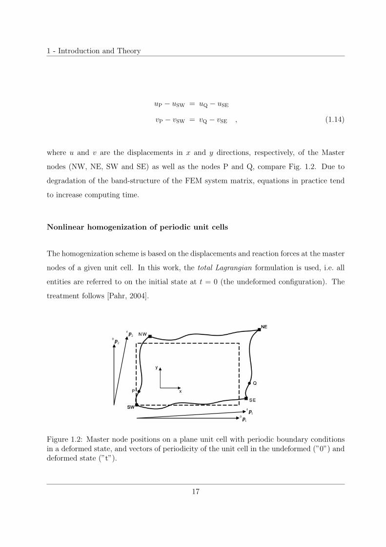
vP − vSW = vQ − vSE , (1.14)
where u and v are the displacements in x and y directions, respectively, of the Master
nodes (NW, NE, SW and SE) as well as the nodes P and Q, compare Fig. 1.2. Due to
degradation of the band-structure of the FEM system matrix, equations in practice tend
to increase computing time.
Nonlinear homogenization of periodic unit cells
The homogenization scheme is based on the displacements and reaction forces at the master
nodes of a given unit cell. In this work, the total Lagrangian formulation is used, i.e. all
entities are referred to on the initial state at t = 0 (the undeformed configuration). The
treatment follows [Pahr, 2004].
1t p
01p
02p
2t p
Figure 1.2: Master node positions on a plane unit cell with periodic boundary conditionsin a deformed state, and vectors of periodicity of the unit cell in the undeformed (”0”) anddeformed state (”t”).
17

1 - Introduction and Theory
As a ”measure” of deformation within a finite strain regime the deformation gradient,
F = F (t), is used. It describes the transformation of a line element d �X in the undeformed
configuration to its deformed state d�x, reading
d�x = Fd �X . (1.15)
For obtaining the deformation gradient in a single material point, the transformations
of three linearly independent line elements are required. For unit cell simulations, these
line elements ideally make up the three edges of the unit cell coincident with the position
vectors of the master nodes. The three individual transformation equations can be written
in a consolidated form, determining the deformation gradient from a deformed state in
tensor notation via
F = dxdX−1 , (1.16)
if the matrices dx = [d�x1, d�x2, d�x3] and dX = [d �X1, d �X2, d �X3] comprise the line elements
as column vectors.
In periodic unit cell analyses, the deformation gradient can be determined by the resulting
displacements t0�ui of the master nodes at time t (left superscript) and referenced to the
undeformed state t = 0 (left subscript), and the three vectors of periodicity of a three-
dimensional unit cell, 0�pi, at t = 0, for i = 1..3, compare Fig. 1.2. The periodicity vectors
for time t read
t�pi = 0�pi +t0 �ui . (1.17)
By using this scheme, the resulting deformation gradient is homogenized within the unit
cell. Substituting the three line elements dx with the periodicity vectors t�pi and dX with
0�pi, Eq. (1.16) yields the deformation gradient t0F , describing deformation at time t as
18
1 - Introduction and Theory
t0F = tp · 0p−1 . (1.18)
An alternative to using the unit cells’ vectors of periodicity is to use the position vectors
of the master nodes.
From the master node displacement vector and the periodicity vectors, the normal vectors
are derived as
�ni = (�pj + �uj) × (�pk + �uk) |i,j,k=1,2,3 ∧ i�=j �=k , (1.19)
each for the deformed and undeformed configurations. The homogenized stress tensor is
then computed from the system of equations
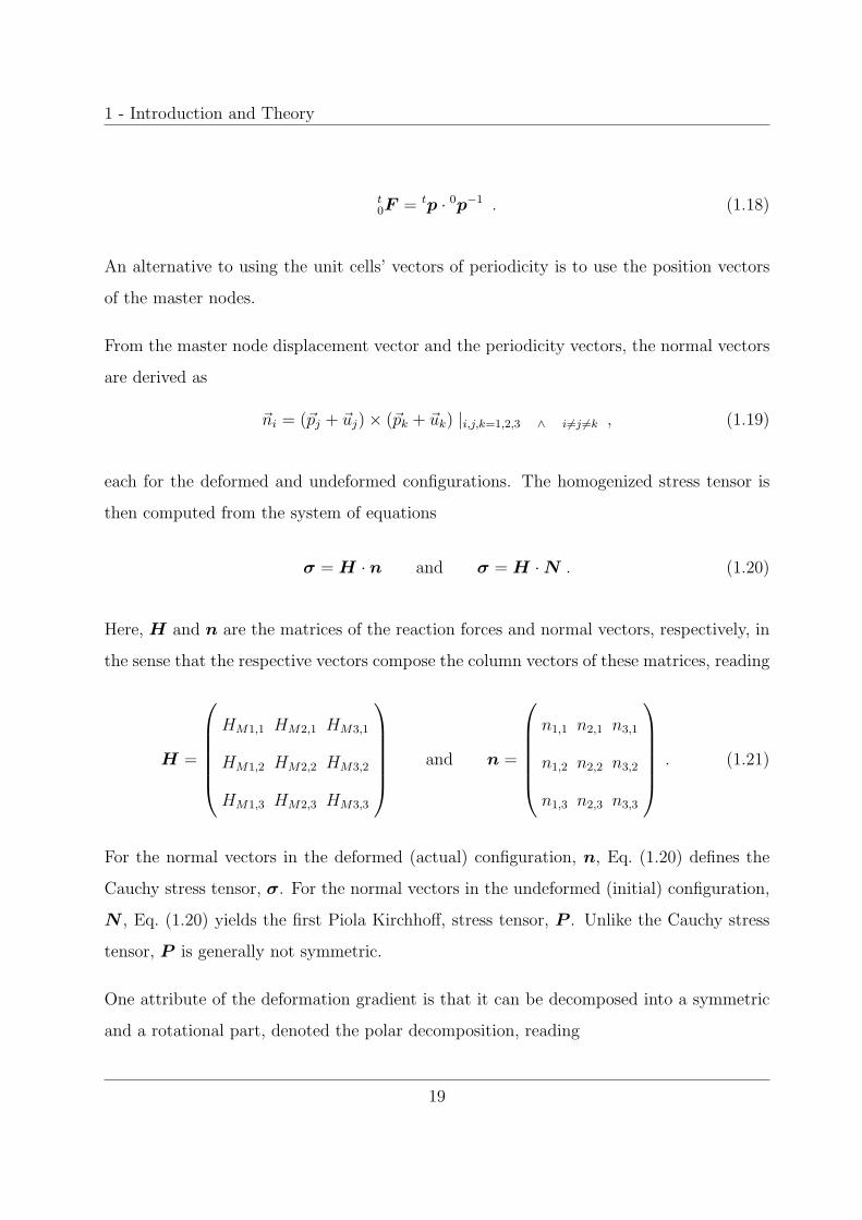
σ = H · n and σ = H · N . (1.20)
Here, H and n are the matrices of the reaction forces and normal vectors, respectively, in
the sense that the respective vectors compose the column vectors of these matrices, reading
H =
⎛⎜⎜⎜⎜⎜⎝
HM1,1 HM2,1 HM3,1
HM1,2 HM2,2 HM3,2
HM1,3 HM2,3 HM3,3
⎞⎟⎟⎟⎟⎟⎠ and n =
⎛⎜⎜⎜⎜⎜⎝
n1,1 n2,1 n3,1
n1,2 n2,2 n3,2
n1,3 n2,3 n3,3
⎞⎟⎟⎟⎟⎟⎠ . (1.21)
For the normal vectors in the deformed (actual) configuration, n, Eq. (1.20) defines the
Cauchy stress tensor, σ. For the normal vectors in the undeformed (initial) configuration,
N , Eq. (1.20) yields the first Piola Kirchhoff, stress tensor, P . Unlike the Cauchy stress
tensor, P is generally not symmetric.
One attribute of the deformation gradient is that it can be decomposed into a symmetric
and a rotational part, denoted the polar decomposition, reading
19

1 - Introduction and Theory
tF = tV tR = tR tU , (1.22)
with V and U denoted as the left and right stretch tensors, respectively, and R being the
rigid body rotation tensor. The deformation state at t can be reached by either stretching
the body with the principal stretches in the principal directions and rotating it afterwards,
or by rotating first and stretching later.
The right Cauchy-Green tensor is defined
C = F T F . (1.23)
A noteworthy attribute of C is its invariance to rotation of the material base. Polar
decomposition and the orthogonality of the rotation, RT = R−1, yield
C = UT RT RU = UT U = U 2 , (1.24)
because U is symmetric. Every symmetric tensor can be formally denoted in terms of a
spectral decomposition. For the right Cauchy-Green tensor this reads
C =3∑
i=1
λ2i · �Ni ⊗ �Ni , (1.25)
with λ2i being the eigenvalues and �Ni the eigenvectors of the respective Eigenvalue problem
C · �Ni = λ2i · �Ni. A symmetric tensor of rank 2 has three real eigenvalues and three principal
directions. The eigenvalues’ physical meaning is the amount of stretching in direction of
the eigenvectors which define the principal directions.
The Green-Lagrange strain tensor, εGL, is defined as
εGL =1
2(F T F − I) . (1.26)
20

1 - Introduction and Theory
By help of the displacement gradient G = F − I this can be expressed as
εGL =1
2(G + GT )︸ ︷︷ ︸
linear
+1
2(G GT )︸ ︷︷ ︸quadratic
, (1.27)
where the first and second summands are the linear and quadratic parts of the strain
tensor, respectively.
The logarithmic strain tensor, εln, is defined as
εln = ln V . (1.28)
Of course, homogenized versions of the individual strain measures are obtained by Eqs. (1.27)
and (1.28) if the deformation gradient is homogenized in the first place, e.g. derived from
the master node displacements of a periodic unit cell as described above.
21

22
Chapter 2
Numerical simulations of the
tribological behavior of Metal Matrix
Composites
Tribology is the science of interactions between contacting surfaces of bodies, moving rela-
tively to each other. These interactions control friction and wear, two important processes
with impact on economic reasoning and long-term reliability. On the one hand, tribologi-
cal knowledge is important for the designer aiming at the reduction of friction and wear1).
On the other hand, it is important for the manufacturer to understand the tribological
background of unwanted friction or excessive wear, in the interest of energy saving, equip-
ment uptime, or life expectancy. Although ‘conventional’ tribology is well established,
the development of new materials requires the understanding of underlying tribological
processes.
1)unless brake systems are to be designed, which require higher coefficients of friction
2 - Tribological Behavior of MMCs
2.1 Tribology basics
2.1.1 Literature review
The importance of contact problems in the field of mechanics is founded in the fact that
contact is one of the most frequently deployed methods of applying loads to a structure or
a body. One unpleasant attribute of contact are unilateral inequalities, which are used to
eliminate tensile tractions at and material penetration of contacting surfaces. If a point
is not in contact, its gap, g, to the counterbody is positive and the contact pressure, p,
is zero2). If the point is indeed in contact, the gap is zero per definition and results in a
positive pressure, reading
g > 0, p = 0, and g = 0, p > 0 . (2.1)
The system of inequalities of Eq.(2.1) serve to determine the points of a surface which are
in contact. In case of a prescribed contact area, the uniqueness of the solution for linear
elastic material has been proved by [Fichera, 1972]. As only relatively simple contact
problems can be treated analytically, numerical methods have evolved and appropriate
algorithms are included in most commercial finite element codes, e.g. [Simulia Inc., 2004].
A discussion on numerical algorithms is found in [Kikuchi and Oden, 1988].
Consideration of friction introduces additional conditions. According to the Coulomb fric-
tion condition [Simulia Inc., 2004; Johnson, 1992]
τeq < τcrit, τcrit = μp , (2.2)
there are two states possible for any point within a contact area. First, the stick condition
(no relative motion), where the magnitude of tangential traction, τeq, is less than the
product of the coefficient of friction (COF), μ, and pressure, p. Secondly, the slip condition
2)Except when adhesion is considered
23

2 - Tribological Behavior of MMCs
(relative motion), where the tangential traction is defined μp. Even though Coulomb
friction is apparently simple, it is difficult to deal with analytically. It certainly helps that
a quasi-static solution can be achieved in many cases where the loading rate is sufficiently
low. In this case the tribological system passes a series of equilibrium states. Sometimes
it is possible to further reduce the problem to a static one for monotonic and proportional
loading. Frictional dissipation at the contact surface also introduces heat into the system,
resulting in a thermomechanical problem. If the dependence of the stress field on the
thermal distortion is zero or low, this can be solved sequentially. In this case, the heat
transfer problem is solved first and the resulting temperature solution is placed into a
stress analysis as a predefined field. Otherwise, a fully coupled thermomechanical problem
has to be solved simultaneously for both the displacement and the temperature degrees of
freedom.
If a thermo-elastic problem is driven by frictional heat generated during sliding, the tem-
perature field at the contacting surface can lead to thermo-elastic instability, giving rise
to wear and other possibly undesired effects. Instabilities of this kind are often found
in brake or clutch systems and are know as frictionally excited thermo-elastic instabilities
(TEI) [Barber, 1969]. A critical sliding speed above which the system is unstable was found
analytically by [Dow and Burton, 1972], who investigated the effect of a small perturbation
on the uniform temperature (or pressure) solution and its growth in time. Recently, sim-
ilar work was done by [Ciavarella and Barber, 2005], who determined the stability range
including a pressure dependent thermal contact resistance and its effect on the frictionally
excited TEI.
2.1.2 Surfaces
A keyword for tribology is surface. Since the interaction takes place on surfaces, the com-
position and state of the involved surfaces as well as the surface near material are of great
influence on the tribological behavior of the system, affecting contact, friction, and wear.
24
2 - Tribological Behavior of MMCs
A solid surface has complex structures and properties depending on the nature of the bulk
material, the method of preparation affecting the surface geometry, and the interaction be-
tween the surface and the environment. The problem with surfaces in tribological processes
is that during experiments, one cannot observe the contact faces during the interaction3),
which makes it necessary to rely on the examination of the surfaces’ states before and after
interaction.
An additional problem is that surface layers contain zones dependent on the bulk material
and forming processes, which can have properties entirely different from the bulk material
(e.g. lightly and heavyly deformed layers, chemically reacted or chemi- and physisorbed
layers). With exception of noble metals, all metals and alloys (and many nonmetals) form
oxide layers in air or layers of nitrides, sulfides, and chlorides in other environments.
Surface roughness
Surface texture is the deviation (random or periodical) from the nominal surface which
includes roughness, waviness, lay, and flaws. Short wavelength roughness is denoted micro-
roughness, whereas waviness (macro-roughness) describes longer wavelengths of asperity
spacing. Lay describes the existence of a principal direction of a predominant surface
pattern, and flaws are randomly distributed, singular deficiencies of the surface.
2.1.3 Friction
Overview
Friction commonly refers to a force resulting from sliding, responsible for an energy trans-
formation in the process, since surfaces in contact usually transmit shear as well as normal
forces across the interface. Generally, there is a correlation between these two force com-
3)except maybe in experiments involving glass as one tribological partner
25
2 - Tribological Behavior of MMCs
ponents. The ‘magnitude’ of friction is often expressed in terms of the COF, μ, which is
given by the frictional force, F , divided by the load, W , pressing two surfaces together,
Eq. (2.3). W is referred to as normal or applied load.
μ =F
W. (2.3)
Note that expressing friction by using a coefficient does not imply the latter to be an in-
trinsic feature of the contributing materials. Every sliding condition produces a different
COF, because of alteration of the participating surfaces over time. Surfaces (especially
metals) tend to oxidize in air, some hydrolyze, or gases are attracted to adsorb. ‘Contami-
nants’ (like water vapor, oil vapor or simply fingerprints) may settle and change the friction
properties considerably. Adsorption and oxidation of solid substrate surfaces takes place
within a time frame of about 10−8s to 10−7s. Consequently, it is difficult to find values
of COFs in publications, which are applicable for the frictional situation and environment
at hand. Most published values have been determined in controlled environments and
narrow ranges of relevant parameters. Although data is usually reliable and reproducible,
it applies only to the environment used within the test. Often only a fixed (single) value
for the COF is given, e.g. 0.2 for (dry) steel against a steel counterbody, neglecting that
one can measure values ranging from 0.1 to 1.2, depending on the sliding conditions and
environmental influences mentioned above.
Ranges of coefficients of friction
General ranges of coefficients of friction can be defined more easily than absolute values,
e.g. [Bhushan, 2001]:
• μ < 0.1 = very low friction — achievable either by rolling or by elastic contact
between surfaces that have low adhesive force between them
26
2 - Tribological Behavior of MMCs
• μ = 0.1 . . . 0.2 = low friction — achievable by fluid film lubrication4)
• μ = 0.2 . . . 0.8 = intermediate friction — usually found with moderately hard mate-
rials not carefully cleaned
• μ > 0.8 = high friction — with soft, well cleaned metal parts
Since plastic deformation will appear in measurements as an increase of the COF, one
important condition for low friction is that the asperities should not be loaded beyond the
elastic limit. Plastic flow in the asperities appears if the traction exceeds this limit. In this
case asperities are likely to be stretched in the direction of sliding, resulting in a rougher
surface, on average, than before. Loosened particles located at the sliding interfaces can
also be the reason for an increase or decrease of the COF. Oxides especially on metals
may come loose during sliding and over time bulk material is removed as well, either by
adhesive tearing or by fatigue failure. Grains of ceramic material are more likely to be
loosened because of the weaker bonding.
2.1.4 Frictional heating
During sliding, mechanical energy is transformed into internal energy or heat [Bhushan,
2001]. As a result, the temperatures of the involved bodies increase. It is known that
frictional heating is concentrated within the real area of contact of the bodies in relative
motion. Theories exist that frictional heating occurs by atomic-scale interactions within
the top atomic layers on the contacting surfaces [Landman et al., 1993], whereas other
investigators state that the energy dissipation takes place in the bulk material beneath the
contact region by plastic deformation processes [Rigney and Hirth, 1979]. Nevertheless,
there is a common agreement that nearly all of the energy dissipated in frictional contacts
is transformed into heat which is entirely5) conducted into the contacting bodies at the
4)note that this represents a different mechanism, which is not considered in this work5)if convection and/or radiation effects can be neglected
27
2 - Tribological Behavior of MMCs
actual contact interface, e.g. [Uetz and Fohl, 1978].
2.1.5 Heat conduction and partitioning
Analytical analysis
Assuming all energy is dissipated as heat on the sliding surface due to friction, the rate of
heat generated per unit area, qdiss, reads
qdiss = μpv (2.4)
where μ is the COF, p the contact pressure and v is the (scalar) relative sliding velocity. If
μ, p, or v vary over the considered contact area, a appropriate differential condition has to
be used. A certain fraction of qdiss enters each of the contacting bodies and induces either a
heat conduction problem within the bodies, a convection problem in case of interaction with
the environment, a temperature rise of the body, a radiation problem, or a combination
thereof. Heat conduction, convection and radiation problems may be treated quasistatically
in the steady state, whereas heating up of a body is a transient process per se.
The conduction of heat within a body is described by the Fourier equation
−k · grad T = �q , (2.5)
wit k being the thermal conductivity, T the temperature, and q the heat flux within the
regarded solid. If one-dimensional variation of temperature is assumed, Eq. 2.5 is reduced
to
−kdT
dx= q . (2.6)
28
2 - Tribological Behavior of MMCs
The task of a thermal analysis is to determine the solution of the appropriate equation
above subject to thermal boundary conditions which include the heat generation equation
(2.4).
In a frictional problem, two bodies have to be considered. Analytical calculation of their
temperatures requires determination of the partitioning of frictionally dissipated heat be-
tween the contacting bodies. The totally generated heat in the interface, qdiss, Eq. (2.4),
is partitioned into the individual heat fluxes q1 and q2, respectively, entering body 1 and
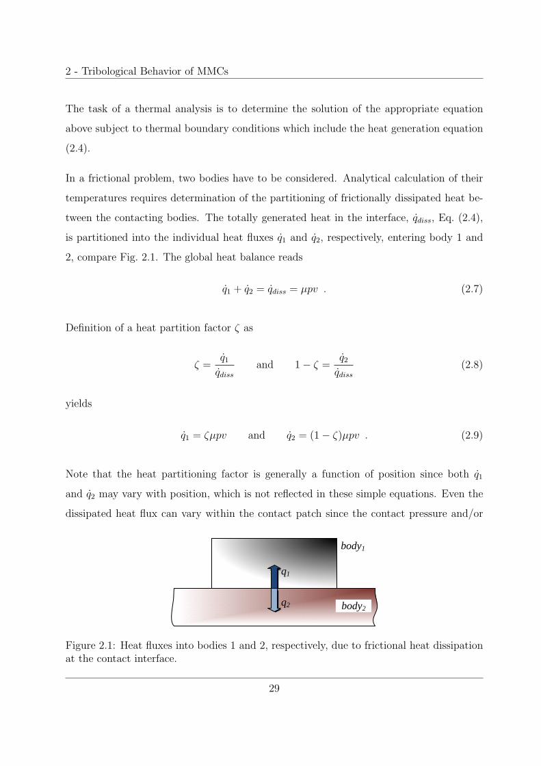
2, compare Fig. 2.1. The global heat balance reads
q1 + q2 = qdiss = μpv . (2.7)
Definition of a heat partition factor ζ as
ζ =q1
qdiss
and 1 − ζ =q2
qdiss
(2.8)
yields
q1 = ζμpv and q2 = (1 − ζ)μpv . (2.9)
Note that the heat partitioning factor is generally a function of position since both q1
and q2 may vary with position, which is not reflected in these simple equations. Even the
dissipated heat flux can vary within the contact patch since the contact pressure and/or
q1
q2
body1
body2
Figure 2.1: Heat fluxes into bodies 1 and 2, respectively, due to frictional heat dissipationat the contact interface.
29
2 - Tribological Behavior of MMCs
relative sliding velocity are not necessarily constant.
There are analytical solutions available for the heat partition function using heat source
methods, which mostly are iterative solutions based on matching the surface temperatures
of the two contacting bodies at all positions within the contact area6). Due to the com-
plexity of these solutions, numerous approximate solutions for the heat partition function
exist, often assuming the heat partitioning to be constant.
Numerical analysis
Many FEM codes facilitate the solution of heat conduction problems. However, in FE
simulations, contrary to analytical solutions, no heat partitioning function needs to be
evaluated. In ABAQUS, only an initial estimate is required as an input from the user. The
temperature distribution in both bodies is then subject to the boundary conditions applied
to the model as well as the thermophysical material properties, resulting in a natural flow
into the contacting bodies. The boundary conditions, in terms of temperatures or heat
fluxes (including the heat source due to frictional dissipation located at the interface) are
responsible for conducting the heat out of the system. In case of simulations with the
counterbody being a rigid body the heat flux into the MMC is stipulated by a defined
partitioning factor.
2.1.6 Wear
Wear is defined as the material removal from a surface due to interaction with another
surface. It is measured in terms of wear rate, which is defined as wear volume per sliding
distance, or in terms of specific wear rate, which is defined as wear volume per sliding
distance and load.
6)If contact is assumed to be ‘perfect’, no temperature jump should be expected across the contactinterface within the real area of contact.
30
2 - Tribological Behavior of MMCs
Wear rates can vary over several orders of magnitude, depending on the operating condi-
tions and materials selection, which suggests that influence on the latter is a key element
for controlling wear. Since wear is a complex system dependent on many variables, wear
rate over a range of test conditions is typically described by multiple wear maps, see e.g.
[Poletti, 2005]. These maps may also contain the change of dominant wear mechanisms
corresponding to the loading situation.
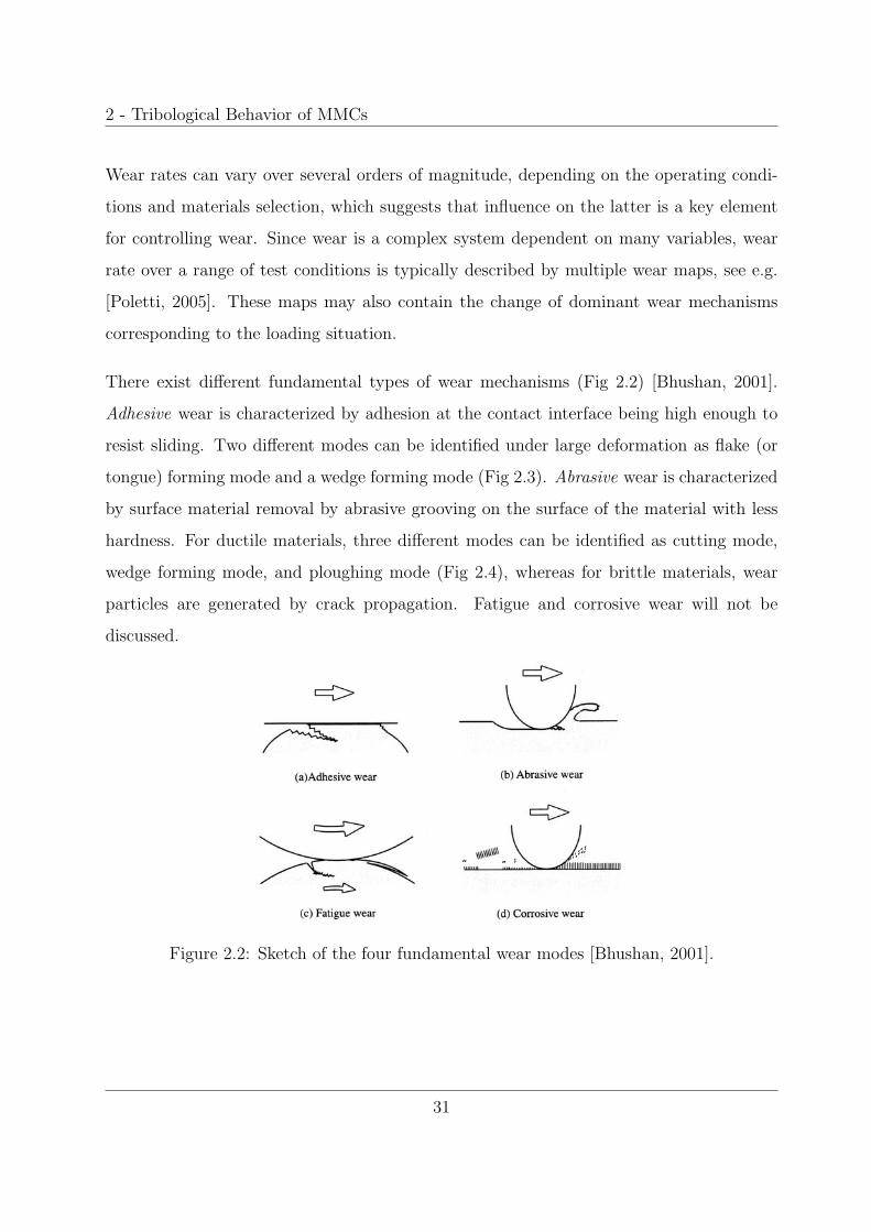
There exist different fundamental types of wear mechanisms (Fig 2.2) [Bhushan, 2001].
Adhesive wear is characterized by adhesion at the contact interface being high enough to
resist sliding. Two different modes can be identified under large deformation as flake (or
tongue) forming mode and a wedge forming mode (Fig 2.3). Abrasive wear is characterized
by surface material removal by abrasive grooving on the surface of the material with less
hardness. For ductile materials, three different modes can be identified as cutting mode,
wedge forming mode, and ploughing mode (Fig 2.4), whereas for brittle materials, wear
particles are generated by crack propagation. Fatigue and corrosive wear will not be
discussed.
Figure 2.2: Sketch of the four fundamental wear modes [Bhushan, 2001].
31

2 - Tribological Behavior of MMCs
Figure 2.3: Schematic adhesive transfer process during wear: adhesive transfer of a thinflake-like particle (a), a wedge-like particle (b) [Bhushan, 2001].
Figure 2.4: Three different modes of abrasive wear observed by SEM: (a) cutting mode ;(b) wedge forming mode; (c) ploughing mode [Bhushan, 2001].
32
2 - Tribological Behavior of MMCs
2.2 Experimental test setup
To provide input for certain process parameters in the analytical calculations as well for the
FE analyses, standard pin-on-ring tribological experiments are performed by cooperation
partner Austrian Research Centers Seibersdorf (ARCS). The test arrangement involves a
pin (diameter 4mm) pressed against a ring (diameter 55mm), which is spinning at varying
speeds for the different measurements. Weights acting on the pin are used for realizing
different, globally constant contact pressures. A sketch as well as a photograph of the test
setup are shown in Fig. 2.5 and Fig. 2.6, respectively. Pin temperatures denoted as T2.5
and T7.5, respectively, are measured at distances of 2.5mm and 7.5mm from the contact
surface. Since these distances decrease during experiments due to wear, a small (linear)
shift in time of the temperature profile along the axis of the pin with respect to the (also
measured) linear wear takes place. The shift is accounted for in experiments with both
high global contact pressure and sliding speed.
Additionally, a thermographic camera is employed to determine the temperature in the
vicinity of the contact surface as well as the global temperature of the ring, TRing. A frame
of the recording is exemplarily shown in Fig. 2.7 (courtesy of Austrian Research Centers
Seibersdorf ). Indicated are also the windows of measurement of the thermal probes.
Other important measured quantities apart from the pin temperatures are the global COF,
μeff , and ring temperature, TRing. For the present investigations, only the global temper-
ature of the ring is of interest. Consequently, the measurement is taken at a sufficient
distance away from the sliding track to ensure a point of the body with no (or very small)
spatial temperature gradient. Although there is heating up on the sliding track of the ring
it is limited spatially and decays long before the same spot on the track reaches the contact
area again.
33

2 - Tribological Behavior of MMCs
Figure 2.5: Schematic of a pin-on-ring experiment; the force pressing the pin onto the ringis denoted W , the ring is spinning with angular velocity ω.
Figure 2.6: A photograph of the pin-on-ring test arrangement [Poletti, 2005].
Figure 2.7: A frame of the recording of the thermographic camera. Also indicated are thewindows of measurement AR01 and AR02, respectively, referring to the location of thethermal probes.
34

2 - Tribological Behavior of MMCs
2.3 Influence of different volume fractions and par-
ticle distributions on the frictional response to a
macroscopic frictional load
The objective in this part of the thesis is, on the one hand, the prediction of the macroscopic
coefficient of friction. On the other hand, the mesocopic and microscopic response is
predicted in terms of stress and strain distributions as a result of frictional loading of
an inhomogeneous material. The influence of different particle volume fractions as well
as distributions in the form of clustering of inhomogeneities is treated. The motivation
behind modelling clusters is that the ”real” materials indeed do not exhibit perfect random
distribution of particles, but have a tendency to develop clustering of inclusions, compare
Fig. 2.8.
Figure 2.8: Scanning-electron microscope image of the distribution of the particles in amaterial; matrix(light), particles(dark) [Poletti, 2005].
35
2 - Tribological Behavior of MMCs
2.3.1 Modeling approach
A modified periodic microfield approach is used to investigate the mechanical and thermal
response of a composite material. The modification results from allowing a free surface
as the contacting surface, not establishing periodicity conditions in this direction. The
macroscopic frictional loading is realized by pressing a counterbody onto a unit cell and
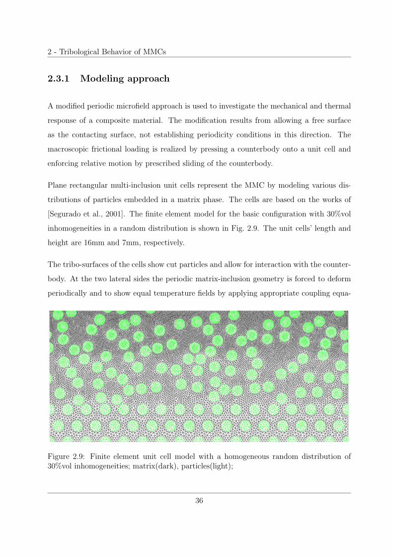
enforcing relative motion by prescribed sliding of the counterbody.
Plane rectangular multi-inclusion unit cells represent the MMC by modeling various dis-
tributions of particles embedded in a matrix phase. The cells are based on the works of
[Segurado et al., 2001]. The finite element model for the basic configuration with 30%vol
inhomogeneities in a random distribution is shown in Fig. 2.9. The unit cells’ length and
height are 16mm and 7mm, respectively.
The tribo-surfaces of the cells show cut particles and allow for interaction with the counter-
body. At the two lateral sides the periodic matrix-inclusion geometry is forced to deform
periodically and to show equal temperature fields by applying appropriate coupling equa-
Figure 2.9: Finite element unit cell model with a homogeneous random distribution of30%vol inhomogeneities; matrix(dark), particles(light);
36

2 - Tribological Behavior of MMCs
tions. The temperature as well as the deformations are fixed at the bottom surface because
from [Segurado et al., 2001] it is evident that the extra effort in special arrangement of
particles and boundary conditions for this model edge is not necessary, as perturbations
of the stress of strain fields on the contact surface decay quickly. Plane stress assumptions
are used. While plane stress models are typically more compliant and plane strain mod-
els exhibit a stiffer behavior than 3D-approaches, the difference in the response regarding
the COF between both planar models using the original cells have been small [Segurado
et al., 2001]. The matrix material as well as the circular particle domains are taken to
behave thermo-elastically. A perfect mechanical and thermal interface between the ma-
trix and its inclusions is assumed. The counterbody is modeled by a rigid body with no
temperature degree of freedom and, consequently, receives no heat during the simulations.
It is assumed that the entire frictionally dissipated heat enters the unit cell (which is in
contrast to subsequent simulations in the next sections where the counterbody gains the
ability to participate in the heat transfer). Each phase has its individual coefficient of
friction with respect to the counterbody. The cells are loaded by applying a macroscopic
contact pressure via the tangentially sliding counterbody. The sliding distance is chosen
such that a steady state is reached in all cases. It is assumed that all energy from the
frictional contact is transformed into heat which is conducted into the contacting bodies
at the actual contact interface, according to a stipulated, constant global heat partitioning
factor. Surface roughness is not directly accounted for but character and condition of the
surfaces are regarded in the local COF of the respective contact pair. Loosened particles
or third body abrasion as well as effects thereof will not be considered in this work.
The Finite Element program ABAQUS [Simulia Inc., 2004] is used for the simulations. Six-
node modified plane stress elements with degrees of freedom for displacements and temper-
atures are used for the simulations. Their modification consists of providing two additional
displacement variables and one additional temperature variable [Simulia Inc., 2004]. The
reason for this choice lies in the problem of second order elements to reproduce contact
37
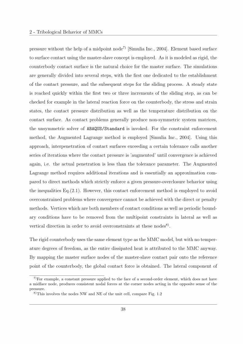
2 - Tribological Behavior of MMCs
pressure without the help of a midpoint node7) [Simulia Inc., 2004]. Element based surface
to surface contact using the master-slave concept is employed. As it is modeled as rigid, the
counterbody contact surface is the natural choice for the master surface. The simulations
are generally divided into several steps, with the first one dedicated to the establishment
of the contact pressure, and the subsequent steps for the sliding process. A steady state
is reached quickly within the first two or three increments of the sliding step, as can be
checked for example in the lateral reaction force on the counterbody, the stress and strain
states, the contact pressure distribution as well as the temperature distribution on the
contact surface. As contact problems generally produce non-symmetric system matrices,
the unsymmetric solver of ABAQUS/Standard is invoked. For the constraint enforcement
method, the Augmented Lagrange method is employed [Simulia Inc., 2004]. Using this
approach, interpenetration of contact surfaces exceeding a certain tolerance calls another
series of iterations where the contact pressure is ’augmented’ until convergence is achieved
again, i.e. the actual penetration is less than the tolerance parameter. The Augmented
Lagrange method requires additional iterations and is essentially an approximation com-
pared to direct methods which strictly enforce a given pressure-overclosure behavior using
the inequalities Eq.(2.1). However, this contact enforcement method is employed to avoid
overconstrained problems where convergence cannot be achieved with the direct or penalty
methods. Vertices which are both members of contact conditions as well as periodic bound-
ary conditions have to be removed from the multipoint constraints in lateral as well as
vertical direction in order to avoid overconstraints at these nodes8).
The rigid counterbody uses the same element type as the MMC model, but with no temper-
ature degrees of freedom, as the entire dissipated heat is attributed to the MMC anyway.
By mapping the master surface nodes of the master-slave contact pair onto the reference
point of the counterbody, the global contact force is obtained. The lateral component of
7)For example, a constant pressure applied to the face of a second-order element, which does not havea midface node, produces consistent nodal forces at the corner nodes acting in the opposite sense of thepressure.
8)This involves the nodes NW and NE of the unit cell, compare Fig. 1.2
38

2 - Tribological Behavior of MMCs
this force is used to determine the global COF by Coulomb’s law.
Varying volume fraction and modeling clustering
The region where particles are to be masked into the matrix randomly9) can be chosen
on the basis of a numbering scheme. With this procedure, it is possible to model various
particle distributions while maintaining randomness. For example, variation in the volume
fraction maintaining random positioning of the inclusions and accumulation of particles in
certain regions by deserting adjacent areas is modeled for the simulations.
2.3.2 Example
Investigations are carried out in order to predict the frictional behavior of Ti-matrices
reinforced by TiC-particles. The Young’s moduli, Poisson’s ratios, coefficients of thermal
expansion, thermal conductivities, and coefficients of friction against steel are listed in
Table 2.1. Temperature-dependent data is not considered in the simulations. The reference
temperature for the temperature rise is (arbitrarily) set to zero degrees.
The simulations are performed for 30%vol and 10%vol, respectively, homogeneous, ran-
domly distributed as well as for 10%vol clustered configurations, compare Fig. 2.10.
An overall contact pressure of 1MPa and a sliding speed of 2mm/s are are used for the
simulations.
9)by assigning matrix properties to the corresponding element sets
39

2 - Tribological Behavior of MMCs
Table 2.1: Thermomechanical properties of matrix and particles
Matrix Particles
Young’s modulus [GPa] 103 440Poisson’s ratio [ - ] 0.3 0.19
Coeff. of therm. expansion [1/K] 9.6E-06 8.0E-06Thermal conductivity [W/mK] 6.5 18
Coeff. of friction against steel [ - ] 0.33 0.6
Figure 2.10: Unit cell models with homogeneous (top) and clustered (bottom) distributionof 10%vol particles.
40

2 - Tribological Behavior of MMCs
2.3.3 Results
Contact pressure and surface traction distribution.
The thermomechanical interaction at and underneath the tribo-surface determines the local
contact pressure distribution and, hence, the local frictional forces. The inhomogeneous
microgeometry generates fluctuation of the contact pressure at the contact surface, compare
Fig. 2.11. The frictional traction distribution is not shown as it is equivalent and only
multiplied by the local COF, accordant to Coulomb’s law. Stress peaks at the particle to
matrix interface are singularities10) caused by modeling a ”perfect” mechanical and thermal
interface using a single node11). For the chosen sliding direction, positive pressure peaks
are caused by transition from a softer to a stiffer material and vice versa.
Figure 2.12 (left) shows the predicted contact pressure over the contact surface for the
10%vol clustered configuration in the steady state condition. In the reinforced region, high
fluctuations are caused by individual particles. Due to the higher stiffness of this region,
the cluster average is higher than the global value of the contact pressure, which is unit
pressure due to the global equilibrium condition. Note that the results are not strictly
periodic because the master nodes NW and NE are members of the contact surface and
consequently have to be taken out of the periodicity equations to avoid overconstraints.
10)The order of the singularities can be determined by, e.g. [Bogy, 1971].11)Using two nodes would require knowledge of the interface properties.
41

2 - Tribological Behavior of MMCs
vcounterbody
Figure 2.11: Contact pressure distribution on the surface of the 30%vol homogeneous,randomly distributed configuration, for an overall contact pressure of 1MPa and slidingspeed 2mm/s.
LOCATION0.0
1.0
2.0
3.0
CO
NT
AC
T P
RE
SS
UR
E [
MP
a]
local fieldglobal averagecluster average
Figure 2.12: Predicted contact pressure for the 10%vol clustered configuration, for anoverall contact pressure of 1MPa and sliding speed 2mm/s.
42

2 - Tribological Behavior of MMCs
Stress state underneath the surface.
The contact interaction at the surface, a combination of unit pressure and sliding, is trans-
ferred into a complex stress and strain state inside the unit cell on the microscale, owing
to the inhomogeneous micro-topology [Segurado et al., 2001]. Due to the higher stiffness
of particles in contrast to the matrix of the present material, ”stress bridges” are devel-
oping in the matrix in regions where particles are queuing. For example, Fig. 2.13(top)
shows the distribution of the von Mises stress in the steady state. Stress concentrations
develop especially in areas of particles having short mean free paths in the direction of the
minimum (in-plane) principal stress. For a detail where these stress bridges in the matrix
between adjacent particles are pronounced compare Fig. 2.13(bottom). In these regions,
the magnitude of stress concentration, in terms of the von Mises stress over the applied
pressure, σ(m)V M/p, is up to 2.5. Consequently, even for an assumed global contact pres-
sure considerably lower than the yield limit of the matrix, plastic yielding12) is introduced
locally in the matrix of the inhomogeneous material.
Since the stiffer particles attract most of the load, the 10%vol clustered configuration has
an increased meso stress level compared to the 30%vol distribution, because the same
load is distributed to fewer particles. This is also reflected in the principal stresses in
the particles, compare Fig. 2.14. As this plane problem is dominated by compression, the
minimum (in-plane) principal stress is the critical one.
Note that the influence of the free surface decays relatively quickly within the unit cell.
Variations of the contact pressure or the surface temperature from the homogeneous distri-
bution decay within a third of the unit cell height, which can be observed also in Fig. 2.15.
12)not considered in these elastic simulations
43

2 - Tribological Behavior of MMCs
Global coefficient of friction.
The predicted macroscopic coefficients of friction are listed in Table 2.2. As the local COF
as well as the Young’s modulus of the particles is higher, the global COF has a tendency
to increase with the particle content. Its value is also influenced by the distribution of
particles, but the difference between clustered and homogeneous random configurations
with the same volume fraction is small. It is noted that the results for the COFs are not
the same compared to derivations from a simple rule of mixture on the macroscopic level.
Figure 2.13: The von-Mises stress distribution (top) for an overall contact pressure of 1MPaand sliding speed 2mm/s; stress concentration in area of particles having short mean freepaths in the direction of the minimum (in-plane) principal stress (bottom).
44
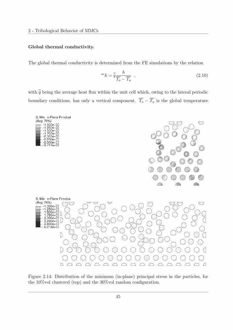
2 - Tribological Behavior of MMCs
Global thermal conductivity.
The global thermal conductivity is determined from the FE simulations by the relation
uck = qh
To − Tu
, (2.10)
with q being the average heat flux within the unit cell which, owing to the lateral periodic
boundary conditions, has only a vertical component. To − Tu is the global temperature
Figure 2.14: Distribution of the minimum (in-plane) principal stress in the particles, forthe 10%vol clustered (top) and the 30%vol random configuration.
45

2 - Tribological Behavior of MMCs
difference over the vertical unit cell dimension, h, in the steady state. The global heat
flux and temperatures are determined by integrating all respective contributions on the
contacting surface, e.g. for the heat flux this reads
q =1
A
∫A
q(x)dA , (2.11)
Figure 2.15: Temperature distribution on the free surface (top), in the matrix (bottom)for the 30%vol homogeneous distribution.
46

2 - Tribological Behavior of MMCs
Table 2.2: Predicted mesoscopic values for the COF, μ, contact pressure, p, heat flux,q, temperature rise, T , and thermal conductivity, k, for the different models and regionswith volume fraction ξ, as predicted by the unit cell simulations. For k, unit cell (UC)predictions as well as Mori-Tanaka (MT) estimations are performed. The asterisk (∗)indicates input values.
ξ μ p q T k
[%] [-] [MPa] [Wm−2] [K] [Wm−1K−1]
UC MT
homogeneous 30 0.420 1.0 0.837 0.676 8.7 8.94
homogeneous 10 0.373 1.0 0.745 0.729 7.16 7.25
clust’d overall 10 0.366 1.0 0.733 0.708 7.16 7.25
plain region 0 0.33∗ 0.909 0.602 0.691 matrix∗ matrix∗
clust. region 30 0.42∗ 1.16 0.964 0.739 8.7∗ 8.94∗
with A being the surface area, dA = 1 · dx for a given planar unit cell.
When comparing the global thermal conductivity as predicted above with Mori-Tanaka
estimates, e.g. [Rammerstorfer and Bohm], a very good agreement is found, compare Table
2.2, even considering the fact that planar cells are confronted with three-dimensional Mori-
Tanaka estimates. The region containing the cluster of the 10%vol configuration, of course,
has the same average thermal conductivity as the 30% configuration.
Frictional dissipation, heat conduction, and surface temperature distribution.
The local contact pressure and the local coefficient of friction determine the frictional heat
dissipation, which acts as thermal loading within a heat transfer analysis solving for the
local temperature fields. At the contact surface of the clustered region considerably more
heat is dissipated due to the combination of a higher contact pressure and higher COF, es-
pecially at the cluster subregion with particles relatively close to each other. This gives rise
to elevated temperatures on the micro as well as the meso-scale despite the higher thermal
conductivity of the particles, and, thus, the higher average (mesoscopic) conductivity in
47
2 - Tribological Behavior of MMCs
the cluster region. The particles attract heat and consequently redirect the vertical heat
flux from an even distribution (homogeneous random distribution) over the unit cell area
to the clustered region on the meso-level, compare Fig. 2.16. On the global scale, as the
total heat flux only varies with the global COF, it scales linearly in the homogeneous and
clustered configurations with the same volume fraction. Figure 2.17(bottom) shows the
distribution of the temperature rise from the ambient temperature at the contact surface
for the clustered cell. The periodic boundary conditions ensure temperature continuity
over the lateral unit cell boundaries. Consequently, also the global heat flux in the hor-
izontal direction vanishes. For the sake of completeness, the temperature as well as the
contact pressure distributions along the contact surface for all particle distributions are
compared in Figs. 2.17 and 2.18.
Note that the temperature fields, together with the phase contrast in thermal expansion,
cause thermally induced stresses. Computation of these stresses lies fully within the capa-
bilities of the models but is not performed for the present material because this effect is of
minor significance.
Due to the limited amount of particles at the surface, several generic unit cells sharing the
same topological descriptors should be investigated and averaged appropriately in order to
obtain quantitatively reliable results [Segurado et al., 2001].
As a consequence of the relatively quick decay of perturbations from the surface, improved
unit cells in terms of computing time should have a larger length-to-height ratio with as
many particles at the surface as possible without a significant loss of quality regarding the
described tasks. This also means that the importance of the periodic boundary conditions
is decreasing.
48
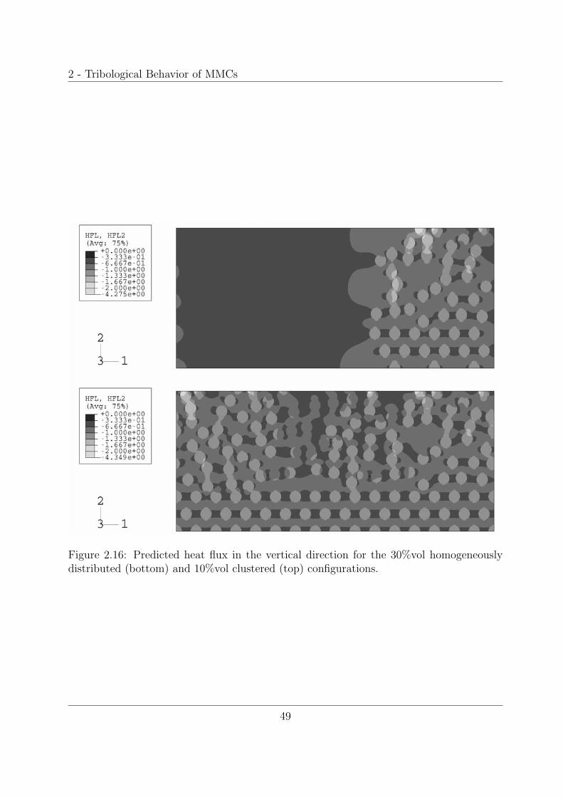
2 - Tribological Behavior of MMCs
Figure 2.16: Predicted heat flux in the vertical direction for the 30%vol homogeneouslydistributed (bottom) and 10%vol clustered (top) configurations.
49
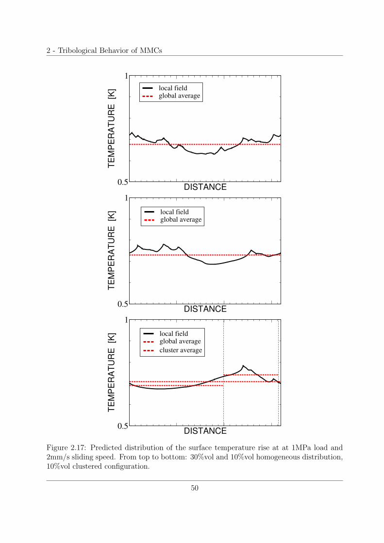
2 - Tribological Behavior of MMCs
Figure 2.17: Predicted distribution of the surface temperature rise at at 1MPa load and2mm/s sliding speed. From top to bottom: 30%vol and 10%vol homogeneous distribution,10%vol clustered configuration.
50

2 - Tribological Behavior of MMCs
Figure 2.18: Predicted contact pressure for the different configurations at 1MPa load and2mm/s sliding speed. From top to bottom: 30%vol and 10%vol homogeneous distribution,10%vol clustered configuration.
51
2 - Tribological Behavior of MMCs
2.4 Analyses of the tribological behavior of MMCs
under consideration of frictionally excited ther-
moelastic instability
The thermoelastic behavior of MMCs in typical frictional contacts is treated by various
approaches. Analytical calculations of a simplified homogenized model accompanying ex-
perimental results serve as an input to Finite Element simulations of the inhomogeneous
MMC. Experimental results from [Poletti et al., 2004] show increased COFs and wear with
higher sliding velocity, which raises the question about the origin of these phenomena. The
effects of frictionally excited thermoelastic instability, associated with thermomechanical
coupling at the contact interface, are investigated and a connection or contribution of TEI
to the aforementioned experimental findings is assessed.
2.4.1 Simplified analytical model
With the simplified analytical model, in combination with the experimental results, certain
unknown process parameters are determined to serve as inputs to the FEM simulations.
In this case, the MMC is treated analytically as a homogenized material. Steady state is
assumed.
Frictional contact
The frictional contact problem involves two bodies in sliding contact. Frictional heat is
dissipated on the contact surface and partitioned between the bodies, subject to material
properties and boundary conditions in temperature or heat flux. The standard experimen-
tal arrangements for measuring friction and wear, pin-on-ring and pin-on-disk, respectively,
comply with this model. For illustration, Fig. 2.19 shows the heat flux distribution from
52

2 - Tribological Behavior of MMCs
the perspective of the pin of a pin-on-ring experiment. A part of the total frictionally
generated heat, qdiss, Eq. (2.4), denoted qpin,out, enters the pin while a contact heat flux,
qcont, is transmitted over the interface. Since no convection or radiation is considered, the
entire heat flux qpin,out leaves the pin into the pin’s mounting. The nature of the heat fluxes
is explained hereafter. Analogous considerations can be made for the ring.
contq�
7.5T
2.5T
,pin outq�
dissq�
ring system
contq�
,ring outq�
pin system
dissqζ �
(1 ) dissqζ− �
Figure 2.19: Heat balance for the pin in the steady state.
2.4.2 Heat fluxes, heat partitioning factor, thermal contact re-
sistance
Assuming all energy is dissipated as heat on the sliding surface, the rate of heat generated
per unit area, qdiss, is given by Eq. (2.4). It has to be partitioned between the contacting
bodies, resulting in the heat fluxes qi for body i = 1, 2. In case of two contacting bod-
ies, using the definition of the heat partition factor, ζ, from Eq. (2.8), these heat fluxes
53
2 - Tribological Behavior of MMCs
are determined with Eq. (2.9). In non-perfect contact, there exists a thermal contact
resistance, which is generally pressure dependent13) (among other possible dependencies).
Consequently, the temperature in opposing points on the contacting surfaces will not match
and a heat flux across the interface orientated towards the lower temperature surface will
develop. If these temperatures are denoted Ti and Tj, respectively, the thermal contact
resistance shall be defined as
R =(Ti − Tj)
qcont
, (2.12)
with qcont being the contact heat flux. Considering a pin-on-ring experiment, the pin is
always the body of higher temperature, regarding its size compared to the ring, the latter
constantly providing fresh, ’cool’ material to the contact zone. In the experiments, the
global temperature of the ring hardly rises above ambient temperature. As a consequence,
the contact heat flux is always directed towards the ring.
If the temperature gradient within a body is known, the heat flux due to conduction is
determined by Eq. (2.5) and reads
�qconduction = −k∇T , (2.13)
with k being the thermal conductivity. The temperature field within the pin is taken
to be homogeneous in the radial direction – hence, one-dimensional, linear temperature
distribution over the length is assumed. In case of the pin-on-ring test setup, the relation
between the temperature distribution and the thermal conductivity of the pin material is
given by Eq. (2.13) and yields
qpin,out = kpin(T2.5 − T7.5)
l, (2.14)
13)A descriptive model for pressure dependency is the ’smoothing out’ of surface asperities with increasingpressure, thus, increasing the real area of contact.
54
2 - Tribological Behavior of MMCs
where T2.5 and T7.5 are the measured pin temperatures, ideally along the axis, with the
distance l in between. Since no radiation or convective effects are considered, all the heat
passing an arbitrary section of the pin is transfered into the mounting.
The heat flux leaving the pin/ring system through the ring, qring,out, is then determined by
qring,out = qdiss − qpin,out . (2.15)
With these equations, the outgoing heat fluxes of pin and ring, qpin,out and qring,out, respec-
tively, can be determined by knowing at least two temperatures along both bodies and
their thermal conductivities.
2.4.3 Heat balance
With the heat fluxes described above, the heat balance can be established. The heat
balance for pin and ring in sliding contact in the steady state, from the perspective of pin
and ring, respectively, and neglecting convection and radiation, reads
ζqdiss = qcont + qpin,out (pin system) (2.16)
(1 − ζ)qdiss = −qcont + qring,out (ring system) , (2.17)
with qpin,out and qring,out being the heat fluxes leaving the bodies through heat sinks, mount-
ing, etc. Summation of these two equations of course yields the heat balance for the entire
system; in this case the contact heat flux cancels out. The thermal contact resistance and
the heat partitioning factor remain unknown so far.
55

2 - Tribological Behavior of MMCs
2.4.4 Derivation of thermal contact resistance and heat parti-
tioning factor
With the above equations, the thermal contact resistance and the heat partitioning factor
are evaluated from pin-on-ring experiments using two methods with differing assumptions.
The first approach involves evaluation of Eq. (2.16) at two different points of time of the
experimental test, assuming that the thermal contact resistance, R, and conductivity, k,
respectively, have not changed significantly, compare Fig. 2.20. The heat balance for the
pin using Eqs. (2.16) and (2.12) reads
ζqdiss =Tpin − Tring
R+
kpin
l(T2.5 − T7.5) , (2.18)
with Tpin being the contact surface temperature average of the pin, computed from the
measured temperatures and the heat conduction equation Eq. (2.13). The temperature
of the ring, Tring, hardly rising above ambient temperature, is known from measurements
with the thermographic camera. Evaluation at two different points in time14), t1 and t2,
yields the following system of two equations with the two unknowns R and ζ.
ζqdiss =Tpin − Tring
R
∣∣∣t1
+kpin
l(T2.5 − T7.5)
∣∣∣t1
ζqdiss =Tpin − Tring
R
∣∣∣t2
+kpin
l(T2.5 − T7.5)
∣∣∣t2
, (2.19)
Solving for the thermal contact resistance yields
R = − l
k
(Tpin − Tring)∣∣∣t1− (Tpin − Tring)
∣∣∣t2
(T1 − T2)∣∣∣t1− (T1 − T2)
∣∣∣t2
. (2.20)
14)In this case, no steady state is assumed.
56
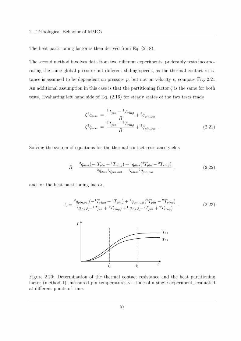
2 - Tribological Behavior of MMCs
The heat partitioning factor is then derived from Eq. (2.18).
The second method involves data from two different experiments, preferably tests incorpo-
rating the same global pressure but different sliding speeds, as the thermal contact resis-
tance is assumed to be dependent on pressure p, but not on velocity v, compare Fig. 2.21
An additional assumption in this case is that the partitioning factor ζ is the same for both
tests. Evaluating left hand side of Eq. (2.16) for steady states of the two tests reads
ζ1qdiss =1Tpin − 1Tring
R+ 1qpin,out
ζ2qdiss =2Tpin − 2Tring
R+ 2qpin,out . (2.21)
Solving the system of equations for the thermal contact resistance yields
R =2qdiss(−1Tpin + 1Tring) + 1qdiss(
2Tpin − 2Tring)2qdiss
1qpin,out − 1qdiss2qpin,out
, (2.22)
and for the heat partitioning factor,
ζ =2qpin,out(−1Tring + 1Tpin) + 1qpin,out(
2Tpin − 2Tring)2qdiss(−1Tpin + 1Tring) +1 qdiss(−2Tpin + 2Tring)
. (2.23)
T2.5
T7.5
t
T
t1 t2
Figure 2.20: Determination of the thermal contact resistance and the heat partitioningfactor (method 1); measured pin temperatures vs. time of a single experiment, evaluatedat different points of time.
57
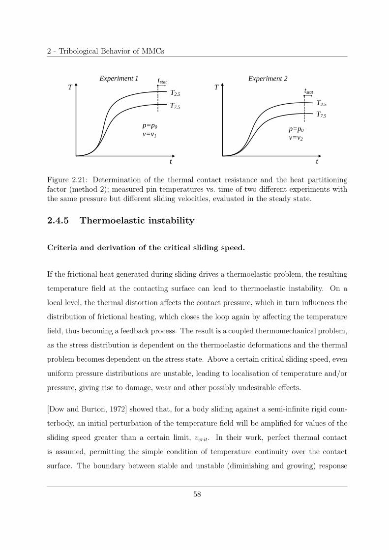
2 - Tribological Behavior of MMCs
T2.5
T7.5
t
T
T2.5
T7.5
t
T
p=p0
v=v1p=p0
v=v2
tstat
tstat
Experiment 1 Experiment 2
Figure 2.21: Determination of the thermal contact resistance and the heat partitioningfactor (method 2); measured pin temperatures vs. time of two different experiments withthe same pressure but different sliding velocities, evaluated in the steady state.
2.4.5 Thermoelastic instability
Criteria and derivation of the critical sliding speed.
If the frictional heat generated during sliding drives a thermoelastic problem, the resulting
temperature field at the contacting surface can lead to thermoelastic instability. On a
local level, the thermal distortion affects the contact pressure, which in turn influences the
distribution of frictional heating, which closes the loop again by affecting the temperature
field, thus becoming a feedback process. The result is a coupled thermomechanical problem,
as the stress distribution is dependent on the thermoelastic deformations and the thermal
problem becomes dependent on the stress state. Above a certain critical sliding speed, even
uniform pressure distributions are unstable, leading to localisation of temperature and/or
pressure, giving rise to damage, wear and other possibly undesirable effects.
[Dow and Burton, 1972] showed that, for a body sliding against a semi-infinite rigid coun-
terbody, an initial perturbation of the temperature field will be amplified for values of the
sliding speed greater than a certain limit, vcrit. In their work, perfect thermal contact
is assumed, permitting the simple condition of temperature continuity over the contact
surface. The boundary between stable and unstable (diminishing and growing) response
58
2 - Tribological Behavior of MMCs
to an initial perturbation reads [Dow and Burton, 1972]
2nπ
ltribo
=μvcritαE
2kpinJ− 2
kring
kpin
√vcrit
πkring
ρcz
, (2.24)
where μ is the COF of the material pair, ltribo and z, respectively, are the length and
width of the contact patch, α is the coefficient of thermal expansion, kring and kpin are
the thermal conductivities of ring and pin, E is the Young’s Modulus of the pin, ρ and
c are mass density and specific heat capacity of the steel ring, J is the percentage of the
frictional dissipation transformed into heat, and n is the wave number.
The critical velocity in absence of wear for frictionally excited thermoelastic instability
(TEI) can then be derived solving for the case of n = 1 (the lowest wave number 2nπ/l),
and assuming 100% heat dissipation (J = 1)
vcrit =4(χ + 2ρckringl
2tribo) − 2
√ρckringl2triboχ + ρ2c2k2
ringl4tribo
πzα2μ2E2l2tribo
,
with χ = π2zαμEkpinltribo
(2.25)
However, instability can also occur because of a pressure dependent thermal contact re-
sistance, also making the heat flux transmitted across the interface dependent on the
pressure. Interaction of these two processes was investigated by [Ciavarella and Barber,
2005], whose criterion can be used in this case. Frictionally excited TEI is expected if the
following inequality is fulfilled
Eα(βμv + γ) > 2(1 − ν)(1 +3.88kpinR0
h) , (2.26)
with the definitions
59
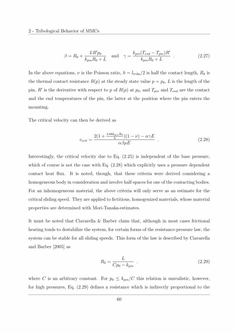
2 - Tribological Behavior of MMCs
β = R0 +LR′p0
kpinR0 + Land γ =
kpin(Tend − Tpin)R′
kpinR0 + L. (2.27)
In the above equations, ν is the Poisson ratio, h = ltribo/2 is half the contact length, R0 is
the thermal contact resistance R(p) at the steady state value p = p0, L is the length of the
pin, R′ is the derivative with respect to p of R(p) at p0, and Tpin and Tend are the contact
and the end temperatures of the pin, the latter at the position where the pin enters the
mounting.
The critical velocity can then be derived as
vcrit =2(1 +
3.88kpinR0
h)(1 − ν) − αγE
αβμE. (2.28)
Interestingly, the critical velocity due to Eq. (2.25) is independent of the base pressure,
which of course is not the case with Eq. (2.28) which explicitly uses a pressure dependent
contact heat flux. It is noted, though, that these criteria were derived considering a
homogeneous body in consideration and involve half-spaces for one of the contacting bodies.
For an inhomogeneous material, the above criteria will only serve as an estimate for the
critical sliding speed. They are applied to fictitious, homogenized materials, whose material
properties are determined with Mori-Tanaka-estimates.
It must be noted that Ciavarella & Barber claim that, although in most cases frictional
heating tends to destabilize the system, for certain forms of the resistance-pressure law, the
system can be stable for all sliding speeds. This form of the law is described by Ciavarella
and Barber [2005] as
R0 =L
Cp0 − kpin
. (2.29)
where C is an arbitrary constant. For p0 ≤ kpin/C this relation is unrealistic, however,
for high pressures, Eq. (2.29) defines a resistance which is indirectly proportional to the
60

2 - Tribological Behavior of MMCs
pressure. If the thermal resistance exhibits a sufficiently rapid decrease with increasing
contact pressure, a stabilizing effect in sliding is found.
2.4.6 Finite element model
The finite element models employed for the simulations are modifications of the models used
in the previous chapter, cf. section 2.3.1, therefore the same general descriptions apply. The
counterbody is treated differently – mechanically, it is still assumed to be rigid, but it gains
the ability to participate in the heat transfer, using the thermophysical material properties
of steel. A constant heat partitioning factor ζ = 3% is assumed for all runs, which is an
input from the combined analytical calculations and experiments. The analytical approach
using a homogenized material determines the various heat fluxes, the thermal contact
resistance, the heat partitioning factor, and estimates for the critical velocity. In previous
experiments [Poletti et al., 2004], the COF of the matrix/steel combination was investigated
at different pressures and sliding velocities. For every simulation, the value of the matrix
COF is adapted to these experimental findings. The FE simulations are carried out with a
pressure and sliding speed of 1MPa and 2mm/s, respectively, which is in the stable regime
(see below), and comparisons with the experiments are done by linear extrapolation of the
dissipated heat, the temperatures as well as stresses.
61

2 - Tribological Behavior of MMCs
2.4.7 Results
Experimental measurements and derived results
Table 2.3 lists the measured and calculated temperatures in the steady state, dependent
on the input parameters global pressure, pexp, and sliding speed, vexp, in the experiments
performed by cooperation partner Austrian Research Centers Seibersdorf. The measured
temperatures are T2.5 and T7.5, respectively, with the indices indicating the approximate
distance in mm from the points of measurement to the contact surface of the pin. Using
linear extrapolation, the contact temperature, Texp, is derived, and an average temperature,
Tavg, between the measured temperatures is defined for comparison purposes only. The
global temperature of the ring is 20◦C for all tests except Test 6, where it is measured as
25◦C. The dissipated heat flux, qdiss, is calculated from the sliding speed, the global COF,
and the applied pressure, compare Eq. (2.4). With Fourier’s law, Eq.(2.5), the outgoing
heat flux of the pin, qpin,out is determined; its fraction of the total dissipated heat flux due
to frictional sliding, qdiss, is listed in the column denoted %Pin. A large fluctuation of this
ratio can be observed here – although in theory the percentage should be approximately
constant, as is assumed in the FE simulations. Fluctuation aside, the comparison yields
a percentage in the range of 1-3%. The table also lists the global measured COF which
includes, but does not distinguish between all dissipative mechanisms of the tribological
system. Tests 3 and 7 show a limited number of results due to technical problems during
the tests.
A limited number of experimental tests is run, which is clearly too low for quantitatively
reliable results but allows for a first estimation of the thermal steady state and the thermal
contact resistance of the material pair by the analytical methods described above.
62
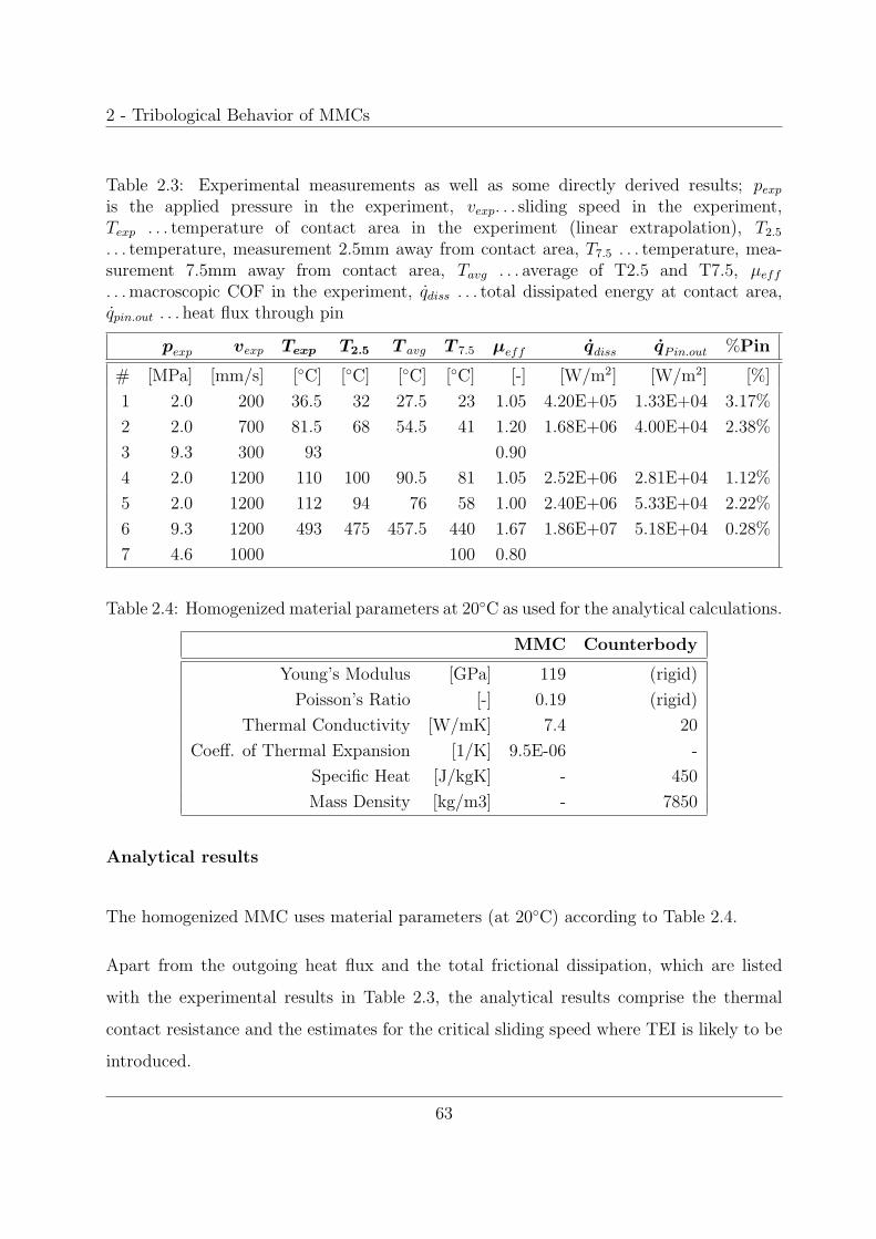
2 - Tribological Behavior of MMCs
Table 2.3: Experimental measurements as well as some directly derived results; pexp
is the applied pressure in the experiment, vexp. . . sliding speed in the experiment,Texp . . . temperature of contact area in the experiment (linear extrapolation), T2.5
. . . temperature, measurement 2.5mm away from contact area, T7.5 . . . temperature, mea-surement 7.5mm away from contact area, Tavg . . . average of T2.5 and T7.5, μeff
. . . macroscopic COF in the experiment, qdiss . . . total dissipated energy at contact area,qpin.out . . . heat flux through pin
pexp vexp Texp T2.5 T avg T 7.5 μeff qdiss qPin.out %Pin
# [MPa] [mm/s] [◦C] [◦C] [◦C] [◦C] [-] [W/m2] [W/m2] [%]
1 2.0 200 36.5 32 27.5 23 1.05 4.20E+05 1.33E+04 3.17%
2 2.0 700 81.5 68 54.5 41 1.20 1.68E+06 4.00E+04 2.38%
3 9.3 300 93 0.90
4 2.0 1200 110 100 90.5 81 1.05 2.52E+06 2.81E+04 1.12%
5 2.0 1200 112 94 76 58 1.00 2.40E+06 5.33E+04 2.22%
6 9.3 1200 493 475 457.5 440 1.67 1.86E+07 5.18E+04 0.28%
7 4.6 1000 100 0.80
Table 2.4: Homogenized material parameters at 20◦C as used for the analytical calculations.
MMC Counterbody
Young’s Modulus [GPa] 119 (rigid)
Poisson’s Ratio [-] 0.19 (rigid)
Thermal Conductivity [W/mK] 7.4 20
Coeff. of Thermal Expansion [1/K] 9.5E-06 -
Specific Heat [J/kgK] - 450
Mass Density [kg/m3] - 7850
Analytical results
The homogenized MMC uses material parameters (at 20◦C) according to Table 2.4.
Apart from the outgoing heat flux and the total frictional dissipation, which are listed
with the experimental results in Table 2.3, the analytical results comprise the thermal
contact resistance and the estimates for the critical sliding speed where TEI is likely to be
introduced.
63
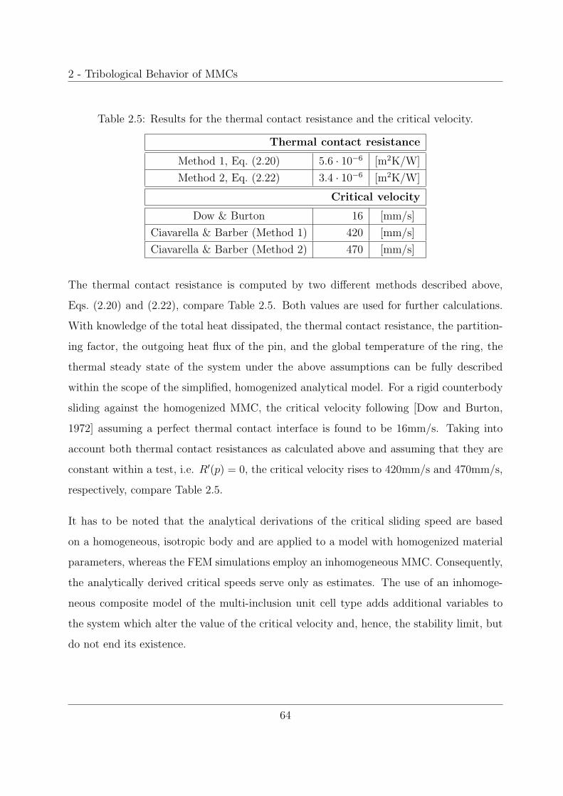
2 - Tribological Behavior of MMCs
Table 2.5: Results for the thermal contact resistance and the critical velocity.
Thermal contact resistance
Method 1, Eq. (2.20) 5.6 · 10−6 [m2K/W]
Method 2, Eq. (2.22) 3.4 · 10−6 [m2K/W]
Critical velocity
Dow & Burton 16 [mm/s]
Ciavarella & Barber (Method 1) 420 [mm/s]
Ciavarella & Barber (Method 2) 470 [mm/s]
The thermal contact resistance is computed by two different methods described above,
Eqs. (2.20) and (2.22), compare Table 2.5. Both values are used for further calculations.
With knowledge of the total heat dissipated, the thermal contact resistance, the partition-
ing factor, the outgoing heat flux of the pin, and the global temperature of the ring, the
thermal steady state of the system under the above assumptions can be fully described
within the scope of the simplified, homogenized analytical model. For a rigid counterbody
sliding against the homogenized MMC, the critical velocity following [Dow and Burton,
1972] assuming a perfect thermal contact interface is found to be 16mm/s. Taking into
account both thermal contact resistances as calculated above and assuming that they are
constant within a test, i.e. R′(p) = 0, the critical velocity rises to 420mm/s and 470mm/s,
respectively, compare Table 2.5.
It has to be noted that the analytical derivations of the critical sliding speed are based
on a homogeneous, isotropic body and are applied to a model with homogenized material
parameters, whereas the FEM simulations employ an inhomogeneous MMC. Consequently,
the analytically derived critical speeds serve only as estimates. The use of an inhomoge-
neous composite model of the multi-inclusion unit cell type adds additional variables to
the system which alter the value of the critical velocity and, hence, the stability limit, but
do not end its existence.
64
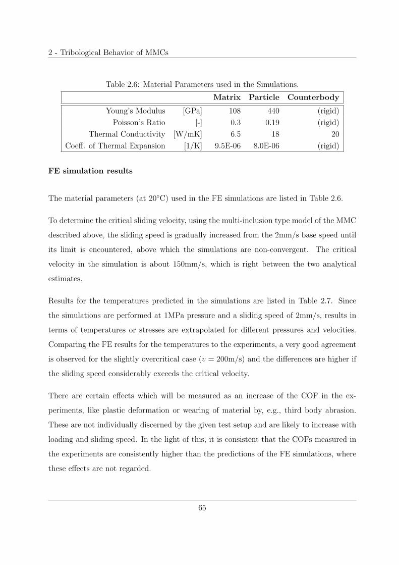
2 - Tribological Behavior of MMCs
Table 2.6: Material Parameters used in the Simulations.
Matrix Particle Counterbody
Young’s Modulus [GPa] 108 440 (rigid)
Poisson’s Ratio [-] 0.3 0.19 (rigid)
Thermal Conductivity [W/mK] 6.5 18 20
Coeff. of Thermal Expansion [1/K] 9.5E-06 8.0E-06 (rigid)
FE simulation results
The material parameters (at 20◦C) used in the FE simulations are listed in Table 2.6.
To determine the critical sliding velocity, using the multi-inclusion type model of the MMC
described above, the sliding speed is gradually increased from the 2mm/s base speed until
its limit is encountered, above which the simulations are non-convergent. The critical
velocity in the simulation is about 150mm/s, which is right between the two analytical
estimates.
Results for the temperatures predicted in the simulations are listed in Table 2.7. Since
the simulations are performed at 1MPa pressure and a sliding speed of 2mm/s, results in
terms of temperatures or stresses are extrapolated for different pressures and velocities.
Comparing the FE results for the temperatures to the experiments, a very good agreement
is observed for the slightly overcritical case (v = 200m/s) and the differences are higher if
the sliding speed considerably exceeds the critical velocity.
There are certain effects which will be measured as an increase of the COF in the ex-
periments, like plastic deformation or wearing of material by, e.g., third body abrasion.
These are not individually discerned by the given test setup and are likely to increase with
loading and sliding speed. In the light of this, it is consistent that the COFs measured in
the experiments are consistently higher than the predictions of the FE simulations, where
these effects are not regarded.
65
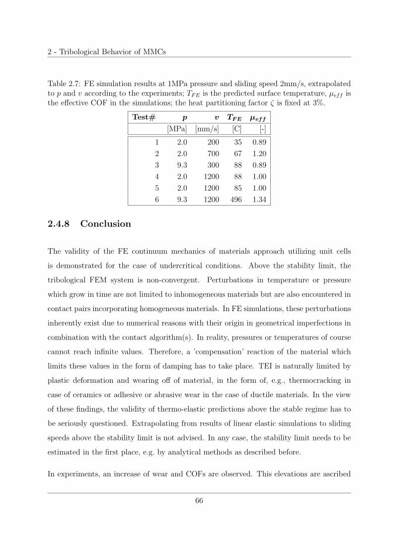
2 - Tribological Behavior of MMCs
Table 2.7: FE simulation results at 1MPa pressure and sliding speed 2mm/s, extrapolatedto p and v according to the experiments; TFE is the predicted surface temperature, μeff isthe effective COF in the simulations; the heat partitioning factor ζ is fixed at 3%.
Test# p v TFE μeff
[MPa] [mm/s] [C] [-]
1 2.0 200 35 0.89
2 2.0 700 67 1.20
3 9.3 300 88 0.89
4 2.0 1200 88 1.00
5 2.0 1200 85 1.00
6 9.3 1200 496 1.34
2.4.8 Conclusion
The validity of the FE continuum mechanics of materials approach utilizing unit cells
is demonstrated for the case of undercritical conditions. Above the stability limit, the
tribological FEM system is non-convergent. Perturbations in temperature or pressure
which grow in time are not limited to inhomogeneous materials but are also encountered in
contact pairs incorporating homogeneous materials. In FE simulations, these perturbations
inherently exist due to numerical reasons with their origin in geometrical imperfections in
combination with the contact algorithm(s). In reality, pressures or temperatures of course
cannot reach infinite values. Therefore, a ’compensation’ reaction of the material which
limits these values in the form of damping has to take place. TEI is naturally limited by
plastic deformation and wearing off of material, in the form of, e.g., thermocracking in
case of ceramics or adhesive or abrasive wear in the case of ductile materials. In the view
of these findings, the validity of thermo-elastic predictions above the stable regime has to
be seriously questioned. Extrapolating from results of linear elastic simulations to sliding
speeds above the stability limit is not advised. In any case, the stability limit needs to be
estimated in the first place, e.g. by analytical methods as described before.
In experiments, an increase of wear and COFs are observed. This elevations are ascribed
66

2 - Tribological Behavior of MMCs
to the effects of TEI, but also to effects of other contributing mechanisms, e.g. plastic
deformation, separation energy, etc. The experimental setup used is not designed to allow
for distinguishing between these effects individually.
The practical consequence for affected tribological systems, operating in the unstable
regime, is that either wear or increased COFs have to be accepted, or a design change
has to be considered. For example, if the thermal contact resistance is either not or weakly
dependent on pressure, neither will the stability limit. In this case, a possible design change
to allow for lower sliding velocities is recommended to avoid or control excessive wear.
67

68
Chapter 3
Forming simulations of MMC
components by a micromechanics
based hierarchical FEM approach
3.1 Introduction
3.1.1 Motivation and scope
Hot forming is an important metal forming technique for semi-finished products. However,
the use of metal matrix composites (MMCs) is constrained by their generally limited forma-
bility. In order to better understand the process and the variables involved, predictions of
the material response to overall loading are of high interest. Computational tools employed
in such predictions are challenged by numerous variables associated with the composition
of the material, e.g. type, volume fraction, sizes, shapes, or distributions of reinforcing
particles. These affect the thermomechanical and physical properties of MMCs, such as
thermo-elastic, elasto-plastic, or conduction properties. On the one hand, modeling tools

3 - Forming Simulations of MMCs
have to be capable of reliably predicting the overall response of the composite based on
the input of the individual properties of the phases, a process denoted as homogenization
in the previous chapters. On the other hand, they have to correctly translate prescribed
macroscopic loads into local responses (localization). Two different approaches are utilized
for homogenization and localization; the Incremental Mori-Tanaka (IMT) as an analyti-
cal constitutive material law based on a mean field approach, and a periodic microfield
approach in form of a unit cell method. As in the previous chapter, investigations are
performed on different length scales in terms of a hierarchical approach.
The present work deals with computational simulations of an elasto-plastic particulate
metal matrix composite undergoing finite strains.
3.1.2 Literature review
There are two widely used approaches in micromechanics of materials. Mean field methods
aim to obtain the overall properties of inhomogeneous materials in terms of phase averages
of the stress and strain fields. They usually give rise to analytical models, and, as a
consequence, pose low computational requirements. They are typically based on Eshelby’s
solution for single ellipsoidal inclusions in an infinite matrix [Eshelby, 1957]. For non-
dilute inclusions, Mori-Tanaka type methods [Mori and Tanaka, 1973; Benveniste, 1987]
allow an efficient evaluation of the thermo-elastic properties of MMCs. When investigating
inhomogeneous materials containing thermo-elasto-plastic constituents, there have been
two main lines of development. On the one hand, the secant plasticity concept has been
applied [Tandon and Weng, 1988] which is limited to radial loading paths in stress space.
On the other hand, incremental plasticity models, such as the incremental Mori-Tanaka
(IMT) method, have been developed [Pettermann et al., 1997] for small strain applications.
An essential feature of the IMT is the capability of accounting for non-radial load paths,
an important prerequisite for its use as a constitutive law. In the elasto-plastic regime,
the IMT typically overestimates overall strain hardening of particulate MMCs, but recent
69
3 - Forming Simulations of MMCs
improvements have been achieved by modifications to the model [Doghri and Ouaar, 2003;
Bornert, 2001] .
The second micromechanical approach comprises evaluation of highly resolved local fields of
a specific microstructure by employing discrete models of its geometry. Periodic microfield
approaches (PMAs) typically employ unit cells to study periodic phase arrangements in
order to limit the computational effort [Bohm, 2002; Bohm et al., 2002]. However, high
resolution discretizations of unit cells containing a number of randomly positioned particles
in a matrix result in large models as well as computation times. Consequently, the PMA
using unit cells is not suited for predicting the response of an entire component, but is
typically employed for computational material characterization.
In this work, both micromechanical approaches for performing homogenization and local-
ization are combined and employed within the framework of the Finite Element Method
(FEM). The IMT method is extended to account for finite strains [Pettermann et al., 2006],
and is used to predict the effective MMC response. The PMA is employed to investigate
the local fields in the matrix and reinforcements, and, by homogenization, the effective
response on the mesoscale. The quality of the results of the analytical IMT approach as
well as its limit of applicability are evaluated by comparing results with predictions from
periodic unit cell models.
3.2 Modeling approach
A hierarchical concept is used, by which the material as well as the component response is
investigated on different length scales. These are defined as
• Macroscale . . . the length scale of the MMC component
• Mesoscale . . . an intermediate length scale where the MMC is regarded as homoge-
70

3 - Forming Simulations of MMCs
nized material
• Microscale . . . the smallest scale which is set by the inclusions’ size
On all scales, constitutive formulations which involve co-rotational Cauchy stresses are
utilized. Since metal plasticity is to be investigated, where the Young’s modulus is typically
several orders of magnitude larger than the yield stress, and, consequently, the elastic
contributions to the strain are very small, logarithmic strains with additive decomposition
of elastic and plastic contribution are used,
ε = εel + εpl . (3.1)
In terms of the deformation gradient, the total deformation is decomposed as
F = F elF pl . (3.2)
The IMT is employed as constitutive material law, implemented into the FEM package
ABAQUS/Standard [Simulia Inc., 2004], in terms of a user-defined subroutine, which can
handle thermo-elastoplasticity as well as temperature dependent material data [Pettermann
et al., 1997, 2006]. An introduction to Mori-Tanaka estimates and the IMT has been given
in chapter 1. The extension from the small strain formulation to finite strains entails the
extension of the matrix constitutive behavior to finite strain J2 metal plasticity and the
handling of the rotations of the material systems. Within the chosen framework, finite
plastic deformations are associated with rotations of the material reference systems at the
micro- as well as the mesoscale. For equi-axed reinforcements these rotations are assumed
to be equal (in the meanfield sense). This implies that the rotation of the matrix phase
is fully conveyed to the embedded linear elastic particles. Inelasticities are confined to
plasticity only and do not account for creep, relaxation or damage.
71

3 - Forming Simulations of MMCs
For the PMA, a multi-particle unit cell is taken from [Bohm et al., 2004]. The cell has
twenty spherical inclusions in a periodic arrangement comprising a particle volume fraction
of 20%, compare Fig. 3.1. Discretization is chosen with respect to the scale of the particles,
resulting in about 50000 elements. Three-dimensional tetrahedral continuum elements with
second-order shape functions are employed. These elements have ten nodes and four Gauss
points and are used in their ”modified” form to prevent volumetric locking. The master
node concept is utilized to apply mesoscopic deformations. It is performed in terms of the
deformation gradient which is suitable as a measure of deformation in the finite deformation
regime. As mesoscopic responses, the master node reactions of the unit cells are evaluated
in terms of co-rotational Cauchy and first Piola Kirchhoff stresses. Evaluation of the highly
resolved microfields is performed statistically and described in terms of histograms. The
latter are probability density distributions htat not only reproduce the frequency of the
classes but also account for their integration point volume is taken into account, since the
latter is not constant for every integration point but, in general, can vary on the order of
one or two magnitudes within the model.
Figure 3.1: The periodic unit cell used in the simulations, with the matrix set semitrans-parent and masked particle mesh.
72
3 - Forming Simulations of MMCs
Both approaches are combined to make use of their individual capabilities and advantages.
The first step in applying the hierarchical concept is the prediction of the components’
response to overall loading by the FEM, employing the IMT as mesoscopic constitutive
material law. Due to its low computational requirements, the IMT is particularly suited for
this task. Further localization is accomplished by this method in terms of phase averages on
the microscale. The components of the deformation gradient are also part of the result. The
second step is accomplished by selection of appropriate locations in the macroscopic model,
extraction of the evolution of the mesoscopic deformation gradients with overall loading,
and application of these deformation histories as mesoscopic loads to the computationally
expensive PMA. The master node coordinates in the deformed configuration can be directly
computed from the definition of the deformation gradient, compare Eq. (1.15), dx = FdX,
if it is written in the form
[d�x1, d�x2, d�x3] = F [d �X1, d �X2, d �X3] , (3.3)
In Eq. (3.3), three line elements make for the column vectors of a matrix in order to
define the deformation gradient of a material point. In this context, the three linearly
independent line elements are understood as those edges of the unit cell that contain the
origin and the master nodes. For the rectangular unit cells used in this work, which are
aligned with the global coordinate system (in the undeformed configuration), coincident
points of origin, and with edge lengths of 1 unit dimension, the master node coordinates
at the actual deformation can directly be seen as the elements of the column vectors of the
deformation gradient, since the undeformed configuration equals the identity matrix.
The respective displacement vectors of the master nodes can be determined by, compare
Eq. (1.17)
[d�u1, d�u2, d�u3] = dx − dX = F − I . (3.4)
73
3 - Forming Simulations of MMCs
This procedure is performed using the program extract F [Luxner, 2007]. The mesoscopic
deformation histories are then applied to the periodic unit cells by prescribing the master
node displacements deducted from the deformation gradient at the selected region of the
model. Since the evolution of the latter is nonlinear with deformation even for simple load
cases, the master nodes follow three independent nonlinear prescribed displacements per
master node.
For the unit cell response, evaluation of tensors as well as scalar fields is done by volume
averaging in the sense of Eq. (1.3), in practice by using approximate numerical quadrature,
compare Eq. (1.13). This can be performed for both phases as well as for individual
particles. As reference volume, the entire phase, e.g. the matrix, individual particle volume,
or the total volume of the unit cell can be chosen. Information on the individual integration
point volumes has to be present in the output database. Such volume averaged fields are
the averages of the deformation gradient F and its rotational part R, the logarithmic
strain tensor (the elastic and plastic part), the accumulated equivalent plastic strain and
the Cauchy stress tensor. In practice, the described steps are performed by the program
deformationanalyzer [Luxner, 2007], which also provides histogram data per integration
point associated with the respective element sets.
Applying mesoscopic deformation histories extracted from the FEM-IMT predictions to the
unit cells gives access to the mesoscopic MMC responses, e.g. the Cauchy stress tensor.
These are used to verify the IMT results attained in the previous step. On the other hand,
the microfields of the PMA are predicted for detailed insight to the matrix and particle
scale. Additionally, they are compared to the IMT’s phase averaged results to assess the
latter’s limits of applicability.
74

3 - Forming Simulations of MMCs
Table 3.1: Elastic material parameters of matrix and particles.
matrix particles
Young’s Modulus [GPa] 100 400Poisson’s Ratio [-] 0.3 0.19
3.3 Example
Simulations are performed on a GleebleR©1)-type experiment, which is a compression test
of a cylindrical specimen between two anvils. The length and diameter of the specimen are
15mm and 10mm, respectively. The model material investigated in this work resembles an
MMC with 20%vol of ceramic particulate inclusions. The particles are assumed to be of
spherical shape and statistically homogeneously distributed. The matrix is taken to behave
elasto-plastically and the inclusions are linear elastic; both phases are isotropic.
The elastic material parameters Young’s moduli E(m) and E(p) as well as the Poisson’s
ratios ν(m) and ν(p) of matrix and particles are listed in Table 3.1. The flow curve of the
matrix material is shown in Fig. 3.2. Associated J2-plasticity and isotropic hardening are
adopted. A perfect interface bonds the individual phases and no damage is assumed to
occur throughout the loading history.
An axisymmetric FEM model for the upper half of the specimen is employed using contin-
uum elements with biquadratic displacement interpolation and reduced integration. The
initial aspect ratio of the elements is set to 2/3 (radial/axial dimension). In Fig. 3.3, the
undeformed, homogeneous mesh is visible at the top. The global deformation applied re-
sembles a reduction in length to 2/3, and is prescribed in the axial direction at the top
edge. To model stiction between specimen and anvil, radial displacements at this edge are
locked.
The FEM simulation of the above sample is carried out with the constitutive behavior
1)Dynamic Systems Inc., Poestenkill, NY
75

3 - Forming Simulations of MMCs
of the MMC described by the IMT. Three locations in the macroscopic model are chosen
(Fig. 3.3) such that a broad spectrum of mesoscopic stress and strain histories is provided
for detailed analysis by the PMA. Location A is the Gauss point closest to the center of
the specimen. Location B is close to the outer surface, and location C represents a region
where shear deformation is expected. The simulations are based on a stress-free initial
state and temperature effects are not regarded.
3.4 Results
3.4.1 Macro response: deformation
The final state of deformation is described by the macroscopic deformation gradient com-
ponent in axial direction, F22 = 2/3. The predicted global deformation of the specimen
in this state is shown in Fig. 3.3; no deformation scaling is used. The stiction condition
between the anvils and the specimen causes barreling. Note that elements at the top right
corner are severely distorted because of the chosen load introduction. However, this region
0.0e+00
1.0e+02
2.0e+02
3.0e+02
4.0e+02
5.0e+02
0 0.1 0.2 0.3 0.4 0.5
true
str
ess
[M
Pa]
logarithmic strain [-]
Figure 3.2: Uniaxial stress-strain curve for the matrix material
76
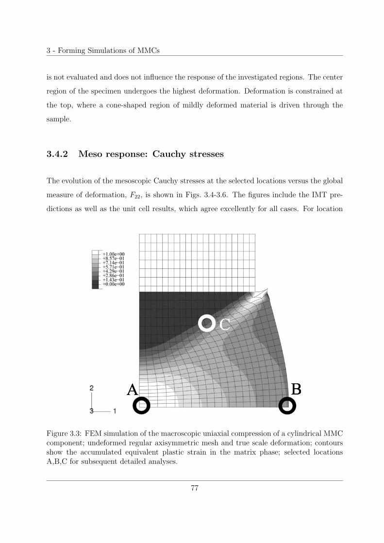
3 - Forming Simulations of MMCs
is not evaluated and does not influence the response of the investigated regions. The center
region of the specimen undergoes the highest deformation. Deformation is constrained at
the top, where a cone-shaped region of mildly deformed material is driven through the
sample.
3.4.2 Meso response: Cauchy stresses
The evolution of the mesoscopic Cauchy stresses at the selected locations versus the global
measure of deformation, F22, is shown in Figs. 3.4-3.6. The figures include the IMT pre-
dictions as well as the unit cell results, which agree excellently for all cases. For location
Figure 3.3: FEM simulation of the macroscopic uniaxial compression of a cylindrical MMCcomponent; undeformed regular axisymmetric mesh and true scale deformation; contoursshow the accumulated equivalent plastic strain in the matrix phase; selected locationsA,B,C for subsequent detailed analyses.
77

3 - Forming Simulations of MMCs
A, the mesoscopic stress histories are close to a uniaxial compressive stress state, showing
some ’hardening’ despite a nearly ideal plastic flow behavior of the MMC material on the
mesoscale. Note that for the PMA prediction, no convergence could be achieved beyond a
macroscopic deformation gradient of F22 = 0.72.
For location B, a biaxial stress state with compression in the axial and tension in the
hoop directions is predicted. Although axial compression is dominant at the macro level,
the meso-stress magnitude in this direction reaches a maximum and then decreases in the
course of deformation, whereas the tensile hoop stress increases steadily. This markedly
non-radial loading history is consistently predicted by the IMT, owing to its incremental
formulation. Region C shows a more general stress state including mesoscopic shear. For
the present stress-strain formulation, this causes rotation of the material reference system.
The resulting deformation of unit cells pertaining to the three locations and the final states
of deformation are displayed in Fig. 3.7, no displacement scaling being used. Note that in
the case of location C the employed unit cell exhibits some mesoscopic strain concentration.
However, this has no influence on the results, which will be explained in the next chapter.
Figure 3.4: Evolution of the mesoscopic Cauchy stress tensor component σ22 over the globaldeformation gradient component for location A, predicted by the IMT and the PMA.
78

3 - Forming Simulations of MMCs
Figure 3.5: Evolution of the mesoscopic Cauchy stress tensor components over the globaldeformation gradient component for location B, predicted by the IMT and the PMA.
Figure 3.6: Evolution of the mesoscopic Cauchy stress tensor components over the globaldeformation gradient component for location C, predicted by the IMT and the PMA.
79
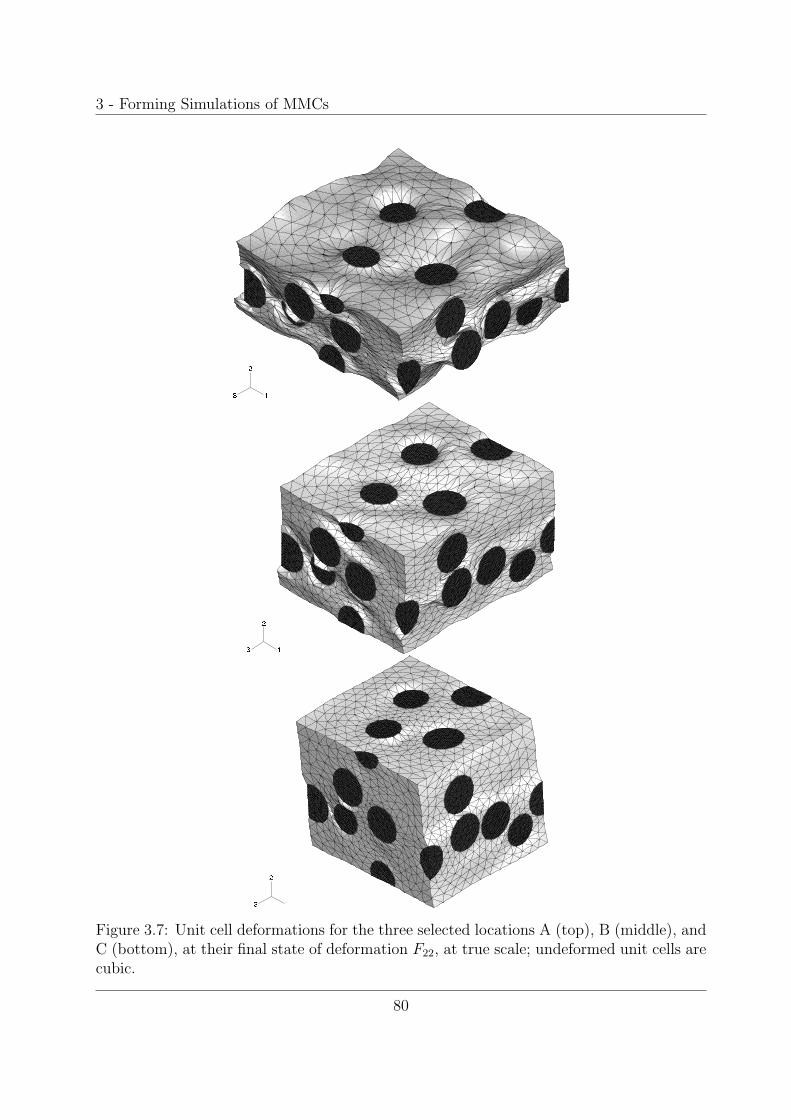
3 - Forming Simulations of MMCs
Figure 3.7: Unit cell deformations for the three selected locations A (top), B (middle), andC (bottom), at their final state of deformation F22, at true scale; undeformed unit cells arecubic.
80

3 - Forming Simulations of MMCs
3.4.3 Micro response
Accumulated equivalent plastic strain in the matrix
The probability density distribution of the accumulated equivalent plastic strain in the
matrix, as predicted by the unit cell simulations at location A, is shown in Fig. 3.8 for the
global deformation gradient F22 = 0.88. Also indicated are its phase average value from
the unit cell, and the prediction by the IMT. The latter is very close to the phase average
obtained from the unit cell. On the microscale, however, the scatter of the accumulated
equivalent plastic strain in the matrix phase is considerable.
0.005
0.045
0.085
0.125
0.165
0.205
0.245
0.285
0.325
0.365
0.405
0.445
0.485
0.525
0.565
0.605
0.645
0.685
0.725
0.765
PMA
IMT
Pro
ba
bil
ity
de
nsit
y
Accumulated equivalent plastic strain
Figure 3.8: Probability density distribution of the accumulated equivalent plastic strain inthe matrix phase as predicted by the unit cell simulations at F22 = 0.88 for location A, itsmean value (PMA), and the IMT prediction.
81
3 - Forming Simulations of MMCs
Maximum principal stresses in the particles
The maximum principal stresses can serve as an indicator for particle fracture. Figures
3.9 and 3.10 show the probability density distribution of the maximum principal stresses
in the particle phase, as predicted by the unit cells, for locations A and B, respectively.
In the figure, only the envelope curves are presented for easier viewing; bin spacing is
5 ·107MPa. Two states in the deformation history are illustrated, described by macroscopic
deformation gradients F22 = 0.988 and F22 = 0.88, respectively. The figures also show
the phase averages from the unit cell and the mesoscopic IMT predictions. It should be
noted that the maximum principal stresses at some Gauss points are outside the displayed
interval. However, the associated volumes are two orders of magnitudes smaller than that
of a particle.
Generally, for both selected regions, the distribution of the maximum principal stresses
shifts towards higher values in course of the deformation. At the same time, its scat-
ter increases. Although location A is associated with a uniaxial compressive stress state
mesoscopically, the unit cell simulation predicts a considerable level of positive maximum
principal stresses in the particles, even at moderate deformation, cf. Fig. 3.9. In fact, par-
ticle fracture in the center of Gleeble tests has been found experimentally [Poletti et al.,
2003]. The IMT severely underestimates the maximum principal stresses; its predictions
are compressive with a value of σI(p) = −20MPa at F22 = 0.988 and close to zero at
F22 = 0.88, respectively.
Rigid body rotations
Figure 3.11 shows the distribution of the rigid body rotations of individual particles within
the unit cell in the 12-plane for location C. The average rotation of all particles as well as
the mesoscopic rotation of the material system are also indicated in the figure. In this case,
the end-state of the simulation is regarded, F22 = 2/3. The rotations of components in
82
3 - Forming Simulations of MMCs
other planes than the 12-plane are at least one order of magnitude smaller. Because of the
much higher Young’s modulus of the particle phase compared to the matrix, deformations
of the particles are small. Therefore, the scatter within individual particles disappears
and the distribution of rotations is represented well by the average rotations of individual
particles.
The good agreement in the averages of the PMA and the IMT as well as the relatively
small scatter in rotation of the individual particles justify the assumption made in the
finite strain formulation of the IMT, compare Section 1.3.3, 12.
Other load cases
Two essential load cases associated with forming are hydrostatic pressure and spatially
homogeneous temperature changes. Due to its formulation, the IMT is not capable of
predicting plastic yielding in these cases. However, unit cell simulations of these load cases
do not show mesoscopic residual strains either, at least not at reasonable loads, compare
Fig. 3.12, which pertains to the triaxial compression (hydrostatic) load case. Consequently,
the IMT maintains its good predictive capabilities on the mesoscale.
All tools are fully prepared to include the thermal expansion, temperature history as well
as the temperature dependence of the material properties in the simulations.
Note that although the adopted flow curve of the matrix almost approaches that of an ide-
ally plastic material, the IMT is capable of utilizing all kinds of hardening curves, including
softening (where, however, mesh dependencies may occur). Several loading scenarios are
performed successfully using strain hardening as well as strain softening, compare also
Section 3.6.
83
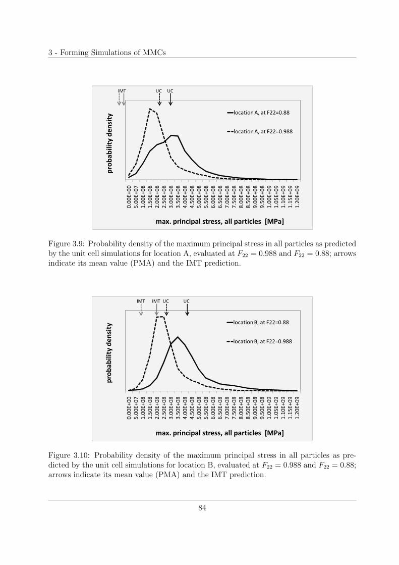
3 - Forming Simulations of MMCs
0.00E+00
5.00E+07
1.00E+08
1.50E+08
2.00E+08
2.50E+08
3.00E+08
3.50E+08
4.00E+08
4.50E+08
5.00E+08
5.50E+08
6.00E+08
6.50E+08
7.00E+08
7.50E+08
8.00E+08
8.50E+08
9.00E+08
9.50E+08
1.00E+09
1.05E+09
1.10E+09
1.15E+09
1.20E+09
max. principal stress, all particles [MPa]
location A, at F22=0.88
location A, at F22=0.988
pro
ba
bil
ity
de
nsi
ty
UCUCIMT
Figure 3.9: Probability density of the maximum principal stress in all particles as predictedby the unit cell simulations for location A, evaluated at F22 = 0.988 and F22 = 0.88; arrowsindicate its mean value (PMA) and the IMT prediction.
0.00E+00
5.00E+07
1.00E+08
1.50E+08
2.00E+08
2.50E+08
3.00E+08
3.50E+08
4.00E+08
4.50E+08
5.00E+08
5.50E+08
6.00E+08
6.50E+08
7.00E+08
7.50E+08
8.00E+08
8.50E+08
9.00E+08
9.50E+08
1.00E+09
1.05E+09
1.10E+09
1.15E+09
1.20E+09
max. principal stress, all particles [MPa]
location B, at F22=0.88
location B, at F22=0.988
pro
ba
bil
ity
de
nsi
ty
UCUCIMTIMT
Figure 3.10: Probability density of the maximum principal stress in all particles as pre-dicted by the unit cell simulations for location B, evaluated at F22 = 0.988 and F22 = 0.88;arrows indicate its mean value (PMA) and the IMT prediction.
84
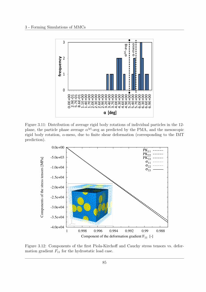
3 - Forming Simulations of MMCs
0
1
2
3
0.0E+00
2.9E-01
5.7E-01
8.6E-01
1.1E+00
1.4E+00
1.7E+00
2.0E+00
2.3E+00
2.6E+00
2.9E+00
3.2E+00
3.4E+00
3.7E+00
4.0E+00
4.3E+00
4.6E+00
4.9E+00
5.2E+00
5.4E+00
5.7E+00
6.0E+00
6.3E+00
6.6E+00
6.9E+00
frequency
α [deg]
α-meso
α(p) -avg
Figure 3.11: Distribution of average rigid body rotations of individual particles in the 12-plane, the particle phase average α(p)-avg as predicted by the PMA, and the mesoscopicrigid body rotation, α-meso, due to finite shear deformation (corresponding to the IMTprediction).
Figure 3.12: Components of the first Piola-Kirchoff and Cauchy stress tensors vs. defor-mation gradient F11 for the hydrostatic load case.
85
3 - Forming Simulations of MMCs
3.4.4 Conclusion
When comparing the IMT results to those of the PMA on the mesoscale, the former’s
predictions are found to be excellent and the assumptions made in the IMT’s formulation
are shown to hold. Predictions on the microscale are limited by the inherent mean field
assumptions, though, and the PMA is still the tool of choice on these length scales.
An advantage of the IMT is, apart from low computational costs in terms of speed and
memory requirements, the possibility to employ a micromechanical constitutive material
law to an entire structure or component. To combine the strengths of both methods for
predicting the response of a macroscopic metal matrix composite component, the following
procedure is suggested. The IMT is employed to provide quick and reliable access to
the material response at the mesoscale, where its predictions render excellent results. As
the periodic microfield approach is computationally very expensive, it is used for selected
regions only if more detail at the fluctuating fields in the phases is required , e.g. to provide
information about the onset of damage, particle fracture or interface delamination.
86

3 - Forming Simulation of MMCs
3.5 Mesoscopic strain concentration/localization in pe-
riodic unit cells
3.5.1 Problem description, identified conditions, and an approach
to prevent mesoscopic strain concentration in the employed
unit cells
The periodic unit cells employed in the finite strain predictions show a distinctive behavior
with load cases involving shear deformation. In this case, certain regions across the unit
cell develop in which the average strain is considerably higher than in other regions of
the unit cell. To illustrate this behavior, the ”simple shear” load case is studied, which is
accomplished by prescribing one of the displacements of master node i, ui, in j direction
(i, j = 1, 2, 3; i �= j)2), e.g. displacement of master node 3 in 2-direction, compare Fig. 3.13.
For the following examples, the prescribed master node displacements are chosen to be
half a unit cell dimension, clearly exceeding the shear deformation of location ”C” in the
previous chapter.
All shear load cases show mesoscopic strain concentration behavior with the employed
periodic unit cells, compare Fig. 3.14, which presents the final deformation state for all
load cases. The accumulated equivalent plastic strain in the region of a plane exhibiting
this behavior is several times higher than the average. Shear in the 13- and 23-planes
exhibits this behavior in a plane near the top (in 3-direction) of the unit cell, compare
Fig. 3.14, middle row left and right, and bottom row right. When the displacements in the
3-direction of master node 2 are prescribed, also resulting in shear in the 23-plane, a plane
near the left face (in 2-direction) is activated, compare bottom row left in the figure. The
unit cell simulations comprising shear in the 12-plane suffer from convergence problems
2)thus, resulting in six sub-load cases
87
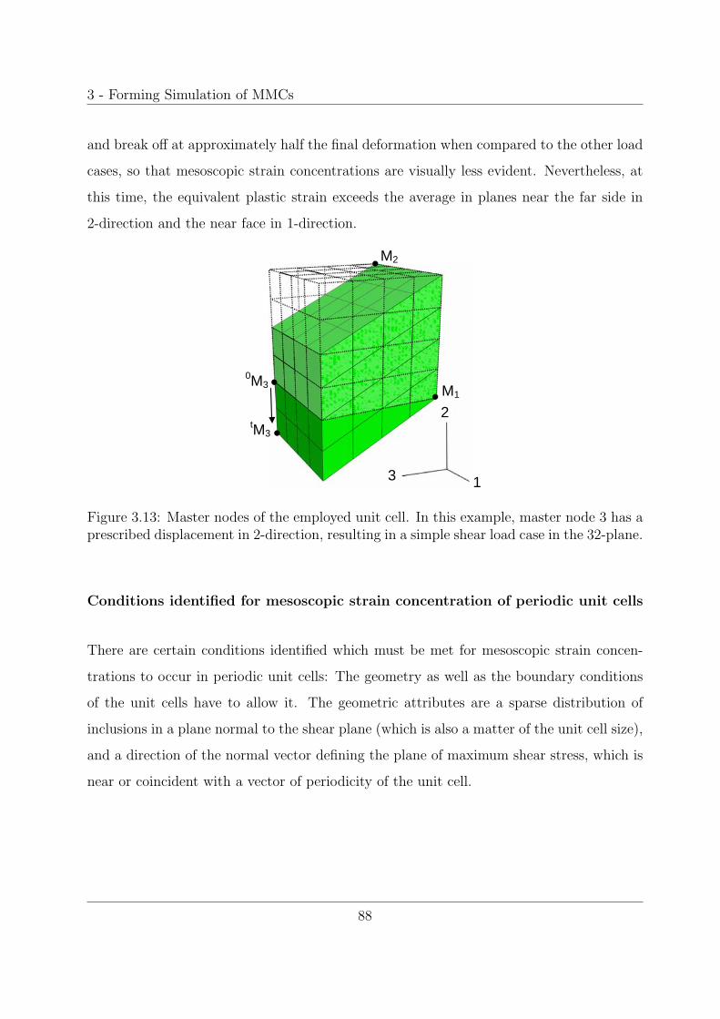
3 - Forming Simulation of MMCs
and break off at approximately half the final deformation when compared to the other load
cases, so that mesoscopic strain concentrations are visually less evident. Nevertheless, at
this time, the equivalent plastic strain exceeds the average in planes near the far side in
2-direction and the near face in 1-direction.
tM3
0M3 M1
M2
2
3 1
Figure 3.13: Master nodes of the employed unit cell. In this example, master node 3 has aprescribed displacement in 2-direction, resulting in a simple shear load case in the 32-plane.
Conditions identified for mesoscopic strain concentration of periodic unit cells
There are certain conditions identified which must be met for mesoscopic strain concen-
trations to occur in periodic unit cells: The geometry as well as the boundary conditions
of the unit cells have to allow it. The geometric attributes are a sparse distribution of
inclusions in a plane normal to the shear plane (which is also a matter of the unit cell size),
and a direction of the normal vector defining the plane of maximum shear stress, which is
near or coincident with a vector of periodicity of the unit cell.
88

3 - Forming Simulation of MMCs
A transformation approach to prevent mesoscopic strain concentration by mak-
ing use of the periodic boundary conditions
The results above indicate that the employed periodic unit cell is too small for the given load
scenarios. Hence, the question arises how to extract any more information within the scope
of the employed tools. The first approach to solve the problem of obviously too small unit
cells is the introduction of ’bigger’3) unit cells comprising higher particle counts. However,
due to the disproportional4) increase in computing time and memory requirements, this is
out of question at the present time. The presented method, on the other hand, utilizes the
same unit cell, but comprises the transformation of the problem to a coordinate system
where the normal to the plane of maximum shear does not coincide with a vector of
periodicity of the unit cell, effectively making use of the periodic boundary conditions
to break one of the conditions mentioned above. Consequently, unit cell simulations are
carried out which transform the evolution of deformation to different coordinate systems
with varying angles of rotation to the original system.
3)bigger in the sense of increased number of particles while maintaining the same discretization standards4)For example, for implicit algorithms, doubling of the cell’s edge lengths, resulting in an increase by a
factor of 8 in its initial volume, would imply roughly 64-times the computing time.
89

3 - Forming Simulation of MMCs
Figure 3.14: The unit cell deformations display mesoscopic strain concentration with simpleshear loading. Top row: 12-plane, obtained by displacement of master node 2 in 1-direction(left) and master node 1 in 2-direction (right). Middle row: 13-plane, with prescribeddisplacement of master node 1 in 3-direction (left) and master node 3 in 1-direction (right).Bottom row: 23-plane, with displacement of master node 2 in 3-direction (left) and masternode 3 in 2-direction (right). Deformations are scaled 1:1.
90
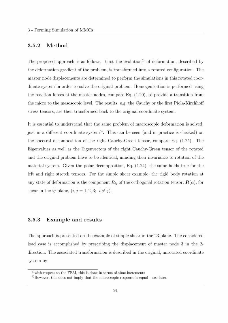
3 - Forming Simulation of MMCs
3.5.2 Method
The proposed approach is as follows. First the evolution5) of deformation, described by
the deformation gradient of the problem, is transformed into a rotated configuration. The
master node displacements are determined to perform the simulations in this rotated coor-
dinate system in order to solve the original problem. Homogenization is performed using
the reaction forces at the master nodes, compare Eq. (1.20), to provide a transition from
the micro to the mesoscopic level. The results, e.g. the Cauchy or the first Piola-Kirchhoff
stress tensors, are then transformed back to the original coordinate system.
It is essential to understand that the same problem of macroscopic deformation is solved,
just in a different coordinate system6). This can be seen (and in practice is checked) on
the spectral decomposition of the right Cauchy-Green tensor, compare Eq. (1.25). The
Eigenvalues as well as the Eigenvectors of the right Cauchy-Green tensor of the rotated
and the original problem have to be identical, minding their invariance to rotation of the
material system. Given the polar decomposition, Eq. (1.24), the same holds true for the
left and right stretch tensors. For the simple shear example, the rigid body rotation at
any state of deformation is the component Rij of the orthogonal rotation tensor, R(α), for
shear in the ij-plane, (i, j = 1, 2, 3; i �= j).
3.5.3 Example and results
The approach is presented on the example of simple shear in the 23-plane. The considered
load case is accomplished by prescribing the displacement of master node 3 in the 2-
direction. The associated transformation is described in the original, unrotated coordinate
system by
5)with respect to the FEM, this is done in terms of time increments6)However, this does not imply that the microscopic response is equal – see later.
91
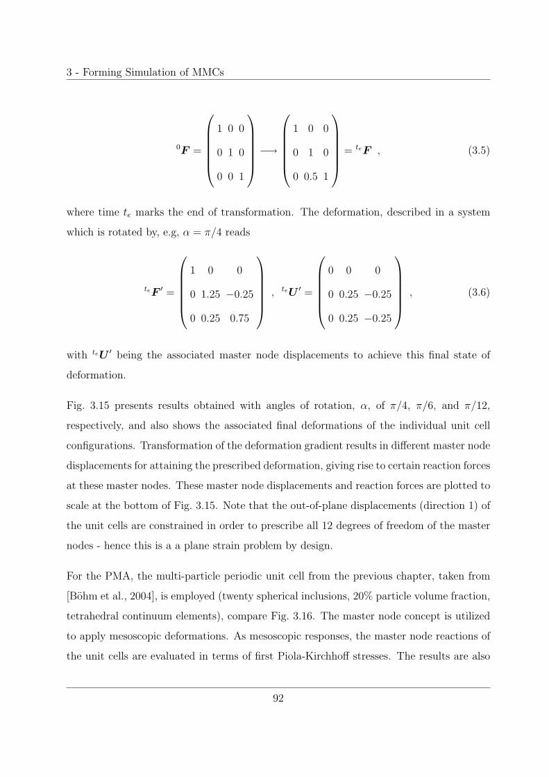
3 - Forming Simulation of MMCs
0F =
⎛⎜⎜⎜⎜⎜⎝
1 0 0
0 1 0
0 0 1
⎞⎟⎟⎟⎟⎟⎠ −→
⎛⎜⎜⎜⎜⎜⎝
1 0 0
0 1 0
0 0.5 1
⎞⎟⎟⎟⎟⎟⎠ = teF , (3.5)
where time te marks the end of transformation. The deformation, described in a system
which is rotated by, e.g, α = π/4 reads
teF ′ =
⎛⎜⎜⎜⎜⎜⎝
1 0 0
0 1.25 −0.25
0 0.25 0.75
⎞⎟⎟⎟⎟⎟⎠ , teU ′ =
⎛⎜⎜⎜⎜⎜⎝
0 0 0
0 0.25 −0.25
0 0.25 −0.25
⎞⎟⎟⎟⎟⎟⎠ , (3.6)
with teU ′ being the associated master node displacements to achieve this final state of
deformation.
Fig. 3.15 presents results obtained with angles of rotation, α, of π/4, π/6, and π/12,
respectively, and also shows the associated final deformations of the individual unit cell
configurations. Transformation of the deformation gradient results in different master node
displacements for attaining the prescribed deformation, giving rise to certain reaction forces
at these master nodes. These master node displacements and reaction forces are plotted to
scale at the bottom of Fig. 3.15. Note that the out-of-plane displacements (direction 1) of
the unit cells are constrained in order to prescribe all 12 degrees of freedom of the master
nodes - hence this is a a plane strain problem by design.
For the PMA, the multi-particle periodic unit cell from the previous chapter, taken from
[Bohm et al., 2004], is employed (twenty spherical inclusions, 20% particle volume fraction,
tetrahedral continuum elements), compare Fig. 3.16. The master node concept is utilized
to apply mesoscopic deformations. As mesoscopic responses, the master node reactions of
the unit cells are evaluated in terms of first Piola-Kirchhoff stresses. The results are also
92
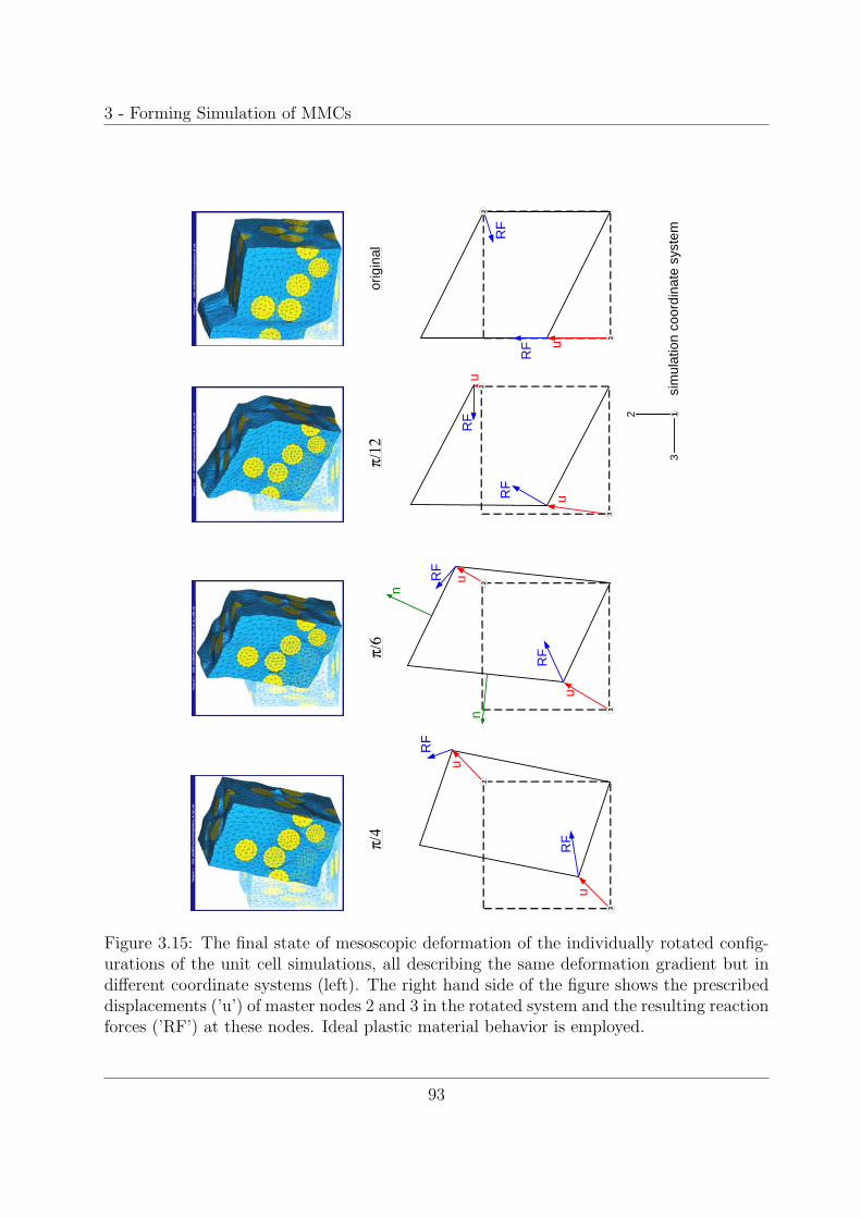
3 - Forming Simulation of MMCs
3
2 1
2
33
RF
RF
RF
RF
u
u
u
22u
u
3
RF
RF
orig
inal
π/4
π/6
n
n
π/12
2
3
RF
RF
sim
ulat
ion
coor
dina
te s
yste
m
u
u
Figure 3.15: The final state of mesoscopic deformation of the individually rotated config-urations of the unit cell simulations, all describing the same deformation gradient but indifferent coordinate systems (left). The right hand side of the figure shows the prescribeddisplacements (’u’) of master nodes 2 and 3 in the rotated system and the resulting reactionforces (’RF’) at these nodes. Ideal plastic material behavior is employed.
93
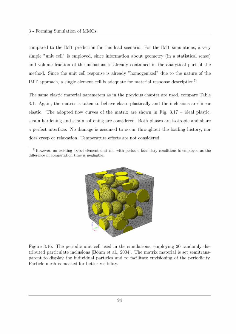
3 - Forming Simulation of MMCs
compared to the IMT prediction for this load scenario. For the IMT simulations, a very
simple ”unit cell” is employed, since information about geometry (in a statistical sense)
and volume fraction of the inclusions is already contained in the analytical part of the
method. Since the unit cell response is already ”homogenized” due to the nature of the
IMT approach, a single element cell is adequate for material response description7).
The same elastic material parameters as in the previous chapter are used, compare Table
3.1. Again, the matrix is taken to behave elasto-plastically and the inclusions are linear
elastic. The adopted flow curves of the matrix are shown in Fig. 3.17 – ideal plastic,
strain hardening and strain softening are considered. Both phases are isotropic and share
a perfect interface. No damage is assumed to occur throughout the loading history, nor
does creep or relaxation. Temperature effects are not considered.
7)However, an existing 4x4x4 element unit cell with periodic boundary conditions is employed as thedifference in computation time is negligible.
Figure 3.16: The periodic unit cell used in the simulations, employing 20 randomly dis-tributed particulate inclusions [Bohm et al., 2004]. The matrix material is set semitrans-parent to display the individual particles and to facilitate envisioning of the periodicity.Particle mesh is masked for better visibility.
94

3 - Forming Simulation of MMCs
Ideal plastic matrix behavior
The resulting unit cell deformations for this load case, comprising ideal plastic matrix
behavior, are presented in Fig. 3.15. The plane of strain concentration can change within
the 23-shear problem even for a moderately small rotation, which can be observed on the
different deformation ’characters’ of the unrotated and the π/12 rotated configuration. For
a rotation of π/6, the strain concentration is somewhat muted and for a rotation of π/4 it is
prevented. No plane normal to the shear plane and coincident with a vector of periodicity
at the same time is sparse enough (in terms of inclusions) to trigger the phenomenon.
The results of the simulations, in terms of the evolution of the components of the first
Piola Kirchhoff stress tensor with deformation, are plotted in Figs. (3.18 - 3.21). Since
the first Piola Kirchhoff stress tensor, P , is unsymmetric, all nine components are plotted.
The smaller of the shear components within the 23-shear plane is coincident with the
respective Cauchy component because the associated reference area does not change. As
the out-of-plane displacement (the 1-direction) of the unit cells is constrained, there are
nonzero components of the stress tensors in the other principal directions since the load
Figure 3.17: Different uniaxial stress-strain curves for the matrix material comprising strainhardening and softening.
95
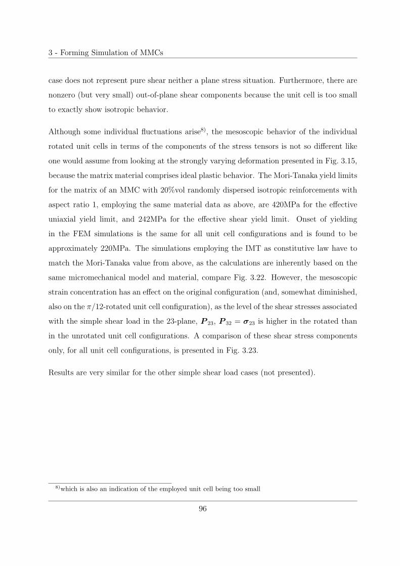
3 - Forming Simulation of MMCs
case does not represent pure shear neither a plane stress situation. Furthermore, there are
nonzero (but very small) out-of-plane shear components because the unit cell is too small
to exactly show isotropic behavior.
Although some individual fluctuations arise8), the mesoscopic behavior of the individual
rotated unit cells in terms of the components of the stress tensors is not so different like
one would assume from looking at the strongly varying deformation presented in Fig. 3.15,
because the matrix material comprises ideal plastic behavior. The Mori-Tanaka yield limits
for the matrix of an MMC with 20%vol randomly dispersed isotropic reinforcements with
aspect ratio 1, employing the same material data as above, are 420MPa for the effective
uniaxial yield limit, and 242MPa for the effective shear yield limit. Onset of yielding
in the FEM simulations is the same for all unit cell configurations and is found to be
approximately 220MPa. The simulations employing the IMT as constitutive law have to
match the Mori-Tanaka value from above, as the calculations are inherently based on the
same micromechanical model and material, compare Fig. 3.22. However, the mesoscopic
strain concentration has an effect on the original configuration (and, somewhat diminished,
also on the π/12-rotated unit cell configuration), as the level of the shear stresses associated
with the simple shear load in the 23-plane, P 23, P 32 = σ23 is higher in the rotated than
in the unrotated unit cell configurations. A comparison of these shear stress components
only, for all unit cell configurations, is presented in Fig. 3.23.
Results are very similar for the other simple shear load cases (not presented).
8)which is also an indication of the employed unit cell being too small
96

3 - Forming Simulation of MMCs
-1.5e+02
-1.0e+02
-5.0e+01
0.0e+00
5.0e+01
1.0e+02
1.5e+02
2.0e+02
2.5e+02
3.0e+02
3.5e+02
0 0.05 0.1 0.15 0.2 0.25 0.3 0.35 0.4 0.45 0.5 0.55
Com
pone
nts,
fir
st P
iola
-Kir
chho
ff s
tres
s te
nsor
[M
Pa]
Component of the deformation gradient F32 [-]
PK11PK22PK33PK12PK21PK13PK31PK23PK32
Figure 3.18: Components of the mesoscopic 1st Piola-Kirchhoff stress tensor vs. the meso-scopic deformation gradient F32 for the original, non-rotated unit cell, for shear stress inthe 23-plane and ideal plastic matrix material. Note that the simulation stops at F32=0.36due to convergence problems caused by excessively distorted elements.
-1.5e+02
-1.0e+02
-5.0e+01
0.0e+00
5.0e+01
1.0e+02
1.5e+02
2.0e+02
2.5e+02
3.0e+02
3.5e+02
0 0.05 0.1 0.15 0.2 0.25 0.3 0.35 0.4 0.45 0.5 0.55
Com
pone
nts,
fir
st P
iola
-Kir
chho
ff s
tres
s te
nsor
[M
Pa]
Component of the deformation gradient F32 [-]
PK11PK22PK33PK12PK21PK13PK31PK23PK32
Figure 3.19: Components of the mesoscopic 1st Piola-Kirchhoff stress tensor vs. the meso-scopic deformation gradient F32 for the π/12-rotated unit cell, for shear stress in the 23-plane and ideal plastic matrix material.
97
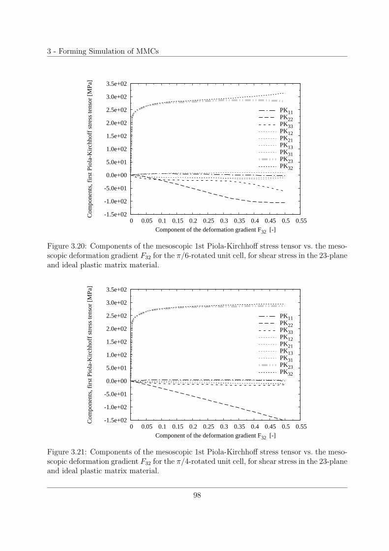
3 - Forming Simulation of MMCs
-1.5e+02
-1.0e+02
-5.0e+01
0.0e+00
5.0e+01
1.0e+02
1.5e+02
2.0e+02
2.5e+02
3.0e+02
3.5e+02
0 0.05 0.1 0.15 0.2 0.25 0.3 0.35 0.4 0.45 0.5 0.55
Com
pone
nts,
fir
st P
iola
-Kir
chho
ff s
tres
s te
nsor
[M
Pa]
Component of the deformation gradient F32 [-]
PK11PK22PK33PK12PK21PK13PK31PK23PK32
Figure 3.20: Components of the mesoscopic 1st Piola-Kirchhoff stress tensor vs. the meso-scopic deformation gradient F32 for the π/6-rotated unit cell, for shear stress in the 23-planeand ideal plastic matrix material.
-1.5e+02
-1.0e+02
-5.0e+01
0.0e+00
5.0e+01
1.0e+02
1.5e+02
2.0e+02
2.5e+02
3.0e+02
3.5e+02
0 0.05 0.1 0.15 0.2 0.25 0.3 0.35 0.4 0.45 0.5 0.55
Com
pone
nts,
fir
st P
iola
-Kir
chho
ff s
tres
s te
nsor
[M
Pa]
Component of the deformation gradient F32 [-]
PK11PK22PK33PK12PK21PK13PK31PK23PK32
Figure 3.21: Components of the mesoscopic 1st Piola-Kirchhoff stress tensor vs. the meso-scopic deformation gradient F32 for the π/4-rotated unit cell, for shear stress in the 23-planeand ideal plastic matrix material.
98
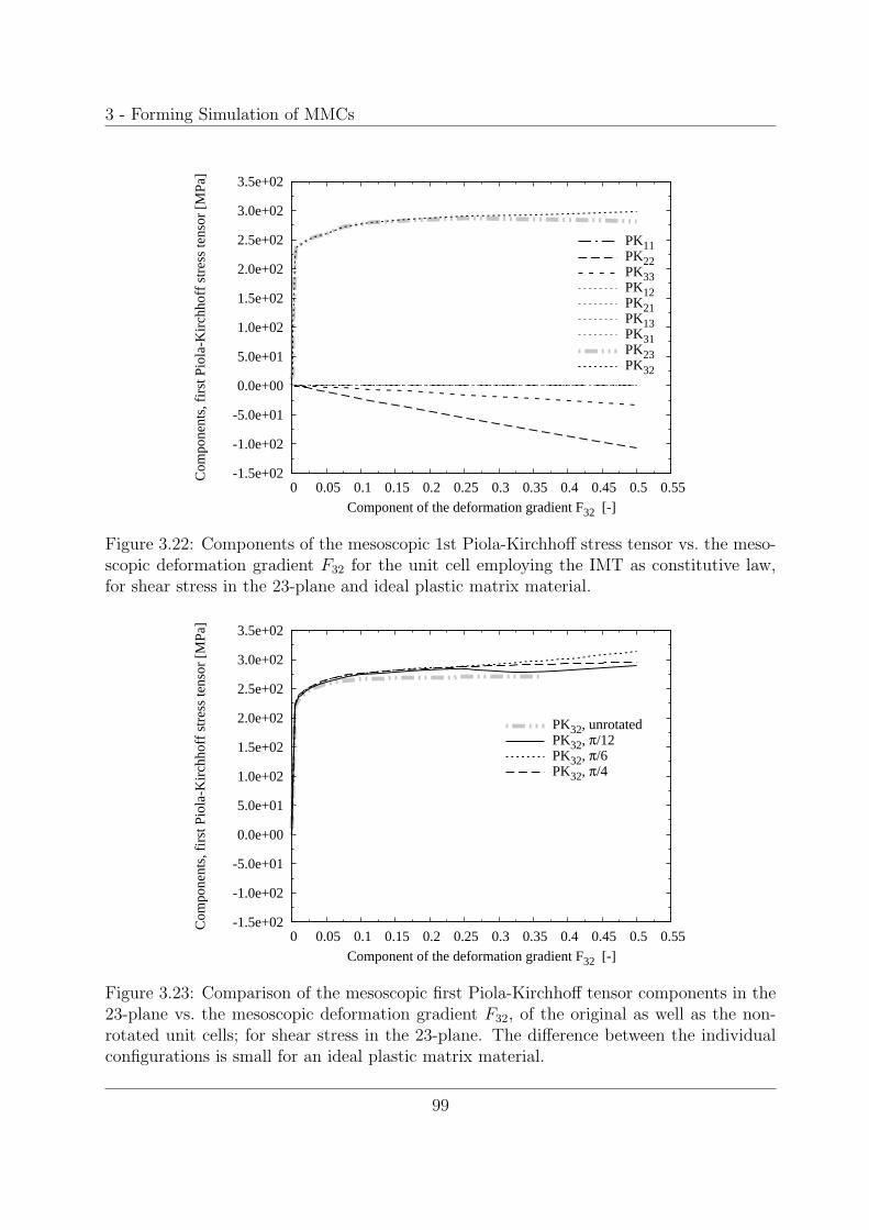
3 - Forming Simulation of MMCs
-1.5e+02
-1.0e+02
-5.0e+01
0.0e+00
5.0e+01
1.0e+02
1.5e+02
2.0e+02
2.5e+02
3.0e+02
3.5e+02
0 0.05 0.1 0.15 0.2 0.25 0.3 0.35 0.4 0.45 0.5 0.55
Com
pone
nts,
fir
st P
iola
-Kir
chho
ff s
tres
s te
nsor
[M
Pa]
Component of the deformation gradient F32 [-]
PK11PK22PK33PK12PK21PK13PK31PK23PK32
Figure 3.22: Components of the mesoscopic 1st Piola-Kirchhoff stress tensor vs. the meso-scopic deformation gradient F32 for the unit cell employing the IMT as constitutive law,for shear stress in the 23-plane and ideal plastic matrix material.
-1.5e+02
-1.0e+02
-5.0e+01
0.0e+00
5.0e+01
1.0e+02
1.5e+02
2.0e+02
2.5e+02
3.0e+02
3.5e+02
0 0.05 0.1 0.15 0.2 0.25 0.3 0.35 0.4 0.45 0.5 0.55
Com
pone
nts,
fir
st P
iola
-Kir
chho
ff s
tres
s te
nsor
[M
Pa]
Component of the deformation gradient F32 [-]
PK32, unrotatedPK32, π/12PK32, π/6PK32, π/4
Figure 3.23: Comparison of the mesoscopic first Piola-Kirchhoff tensor components in the23-plane vs. the mesoscopic deformation gradient F32, of the original as well as the non-rotated unit cells; for shear stress in the 23-plane. The difference between the individualconfigurations is small for an ideal plastic matrix material.
99
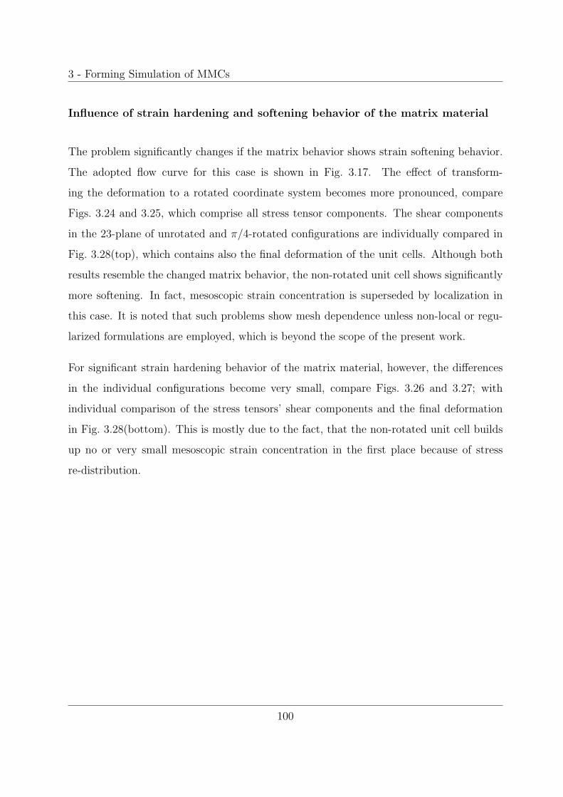
3 - Forming Simulation of MMCs
Influence of strain hardening and softening behavior of the matrix material
The problem significantly changes if the matrix behavior shows strain softening behavior.
The adopted flow curve for this case is shown in Fig. 3.17. The effect of transform-
ing the deformation to a rotated coordinate system becomes more pronounced, compare
Figs. 3.24 and 3.25, which comprise all stress tensor components. The shear components
in the 23-plane of unrotated and π/4-rotated configurations are individually compared in
Fig. 3.28(top), which contains also the final deformation of the unit cells. Although both
results resemble the changed matrix behavior, the non-rotated unit cell shows significantly
more softening. In fact, mesoscopic strain concentration is superseded by localization in
this case. It is noted that such problems show mesh dependence unless non-local or regu-
larized formulations are employed, which is beyond the scope of the present work.
For significant strain hardening behavior of the matrix material, however, the differences
in the individual configurations become very small, compare Figs. 3.26 and 3.27; with
individual comparison of the stress tensors’ shear components and the final deformation
in Fig. 3.28(bottom). This is mostly due to the fact, that the non-rotated unit cell builds
up no or very small mesoscopic strain concentration in the first place because of stress
re-distribution.
100
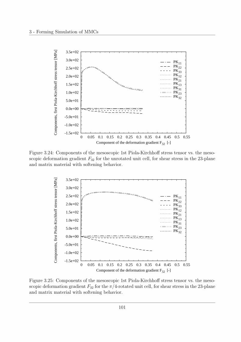
3 - Forming Simulation of MMCs
-1.5e+02
-1.0e+02
-5.0e+01
0.0e+00
5.0e+01
1.0e+02
1.5e+02
2.0e+02
2.5e+02
3.0e+02
3.5e+02
0 0.05 0.1 0.15 0.2 0.25 0.3 0.35 0.4 0.45 0.5 0.55
Com
pone
nts,
fir
st P
iola
-Kir
chho
ff s
tres
s te
nsor
[M
Pa]
Component of the deformation gradient F32 [-]
PK11PK22PK33PK12PK21PK13PK31PK23PK32
Figure 3.24: Components of the mesoscopic 1st Piola-Kirchhoff stress tensor vs. the meso-scopic deformation gradient F32 for the unrotated unit cell, for shear stress in the 23-planeand matrix material with softening behavior.
-1.5e+02
-1.0e+02
-5.0e+01
0.0e+00
5.0e+01
1.0e+02
1.5e+02
2.0e+02
2.5e+02
3.0e+02
3.5e+02
0 0.05 0.1 0.15 0.2 0.25 0.3 0.35 0.4 0.45 0.5 0.55
Com
pone
nts,
fir
st P
iola
-Kir
chho
ff s
tres
s te
nsor
[M
Pa]
Component of the deformation gradient F32 [-]
PK11PK22PK33PK12PK21PK13PK31PK23PK32
Figure 3.25: Components of the mesoscopic 1st Piola-Kirchhoff stress tensor vs. the meso-scopic deformation gradient F32 for the π/4-rotated unit cell, for shear stress in the 23-planeand matrix material with softening behavior.
101

3 - Forming Simulation of MMCs
-1.5e+02
-1.0e+02
-5.0e+01
0.0e+00
5.0e+01
1.0e+02
1.5e+02
2.0e+02
2.5e+02
3.0e+02
3.5e+02
0 0.05 0.1 0.15 0.2 0.25 0.3 0.35 0.4 0.45 0.5 0.55
Com
pone
nts,
fir
st P
iola
-Kir
chho
ff s
tres
s te
nsor
[M
Pa]
Component of the deformation gradient F32 [-]
PK11PK22PK33PK12PK21PK13PK31PK23PK32
Figure 3.26: Components of the mesoscopic 1st Piola-Kirchhoff stress tensor vs. the meso-scopic deformation gradient F32 for the unrotated unit cell, for shear stress in the 23-planeand matrix material with strain hardening behavior.
-1.5e+02
-1.0e+02
-5.0e+01
0.0e+00
5.0e+01
1.0e+02
1.5e+02
2.0e+02
2.5e+02
3.0e+02
3.5e+02
0 0.05 0.1 0.15 0.2 0.25 0.3 0.35 0.4 0.45 0.5 0.55
Com
pone
nts,
fir
st P
iola
-Kir
chho
ff s
tres
s te
nsor
[M
Pa]
Component of the deformation gradient F32 [-]
PK11PK22PK33PK12PK21PK13PK31PK23PK32
Figure 3.27: Components of the mesoscopic 1st Piola-Kirchhoff stress tensor vs. deforma-tion gradient F32 for the π/4-rotated unit cell, for shear stress in the 23-plane and matrixmaterial with strain hardening behavior.
102

3 - Forming Simulation of MMCs
Figure 3.28: Comparison of the components 23 and 32 of the mesoscopic Piola-Kirchhoff 1stress tensor vs. the mesoscopic deformation gradient F32, for shear stress in the 23-plane.The matrix shows strain softening (top) or strain hardening (bottom), and unit cell defor-mation is shown for the unrotated (left) and π/4-rotated (right) configuration, respectively.
103

3 - Forming Simulation of MMCs
3.5.4 Conclusion
Concerns arise how the results are to be interpreted. The question which is the bet-
ter or more accurate solution cannot be answered satisfactorily, as it is conceivable that
mesoscopic strain concentration may well be a valid response of the actual material. The
transformation approach makes use of the boundary conditions to the effect that meso-
scopic strain concentration is in fact ’filtered’, because a concentration band running across
the unit cell is only possible for certain angles of rotation. For periodic unit cells these
angles are 0, π/4, and π/2. Thus, new constraints are introduced to the unit cell via the
periodic boundary conditions, which are angular dependent. The equality in the meso-
scopic deformation does not imply that the underlying microfields are equal as well, which
shows in the – dependent on matrix behavior – noticeable differences of the individual
configurations. If a material model comprising damage or failure is employed for one of
the constituents, which is sensitive to variations in the microfields, a significant difference
in the behavior of the rotated configurations is expected. However, the present method is
a practical approach for obtaining the unit cells’ homogenized behavior.
A conclusion that most certainly can be drawn from the of from the simulations is that
the employed unit cell is too small for load scenarios considerably immersing into the finite
strain regime.
104
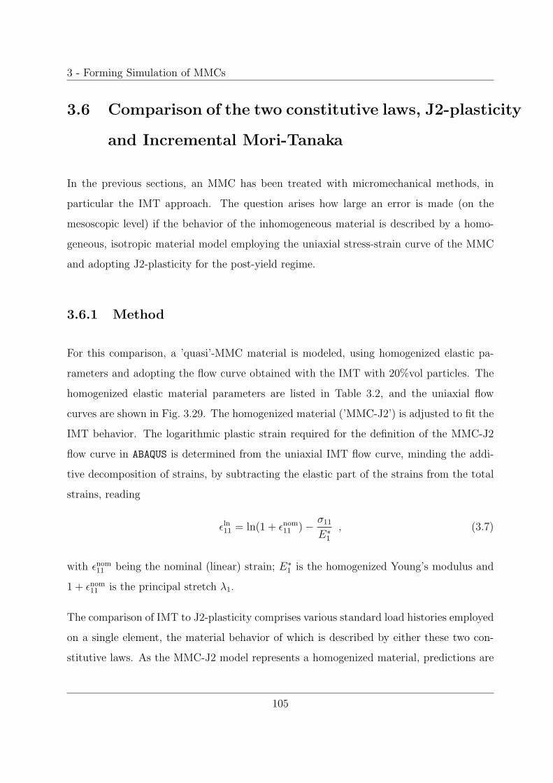
3 - Forming Simulation of MMCs
3.6 Comparison of the two constitutive laws, J2-plasticity
and Incremental Mori-Tanaka
In the previous sections, an MMC has been treated with micromechanical methods, in
particular the IMT approach. The question arises how large an error is made (on the
mesoscopic level) if the behavior of the inhomogeneous material is described by a homo-
geneous, isotropic material model employing the uniaxial stress-strain curve of the MMC
and adopting J2-plasticity for the post-yield regime.
3.6.1 Method
For this comparison, a ’quasi’-MMC material is modeled, using homogenized elastic pa-
rameters and adopting the flow curve obtained with the IMT with 20%vol particles. The
homogenized elastic material parameters are listed in Table 3.2, and the uniaxial flow
curves are shown in Fig. 3.29. The homogenized material (’MMC-J2’) is adjusted to fit the
IMT behavior. The logarithmic plastic strain required for the definition of the MMC-J2
flow curve in ABAQUS is determined from the uniaxial IMT flow curve, minding the addi-
tive decomposition of strains, by subtracting the elastic part of the strains from the total
strains, reading
εln11 = ln(1 + εnom
11 ) − σ11
E∗1
, (3.7)
with εnom11 being the nominal (linear) strain; E∗
1 is the homogenized Young’s modulus and
1 + εnom11 is the principal stretch λ1.
The comparison of IMT to J2-plasticity comprises various standard load histories employed
on a single element, the material behavior of which is described by either these two con-
stitutive laws. As the MMC-J2 model represents a homogenized material, predictions are
105

3 - Forming Simulation of MMCs
Table 3.2: Homogenized elastic material parameters for the MMC material.
Young’s Modulus E∗ [GPa] 127
Poisson’s Ratio ν∗ [-] 0.28
Yield stress σy [MPa] 420
restricted to the mesoscale.
3.6.2 Example, mesoscopic results, and conclusion
Several load cases are considered. A biaxial stress state is achieved by prescribing dis-
placements in 1- and 2-direction, u1 = u2 (a radial load path), resulting in tensile stress
σ11 = σ22 in the respective directions, compare Fig. 3.30. Prescribing the displacement
in 1-direction, −u1, and constraining displacements in 2-direction results in pressure in 1-
and 2-directions, defining a confined compression, compare Fig. 3.31. Uniaxial strain is
Figure 3.29: Flow curves of the investigated materials for the uniaxial stress load case. TheMMC is described by J2-plasticity (MMC-J2), fitted to the IMT uniaxial behavior. Forcomparison, the respective behavior of the matrix material, IMT(0%p), is also presented.
106
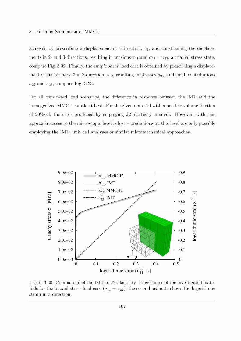
3 - Forming Simulation of MMCs
achieved by prescribing a displacement in 1-direction, u1, and constraining the displace-
ments in 2- and 3-directions, resulting in tensions σ11 and σ22 = σ33, a triaxial stress state,
compare Fig. 3.32. Finally, the simple shear load case is obtained by prescribing a displace-
ment of master node 3 in 2-direction, u32, resulting in stresses σ23, and small contributions
σ22 and σ33, compare Fig. 3.33.
For all considered load scenarios, the difference in response between the IMT and the
homogenized MMC is subtle at best. For the given material with a particle volume fraction
of 20%vol, the error produced by employing J2-plasticity is small. However, with this
approach access to the microscopic level is lost – predictions on this level are only possible
employing the IMT, unit cell analyses or similar micromechanical approaches.
Figure 3.30: Comparison of the IMT to J2-plasticity. Flow curves of the investigated mate-rials for the biaxial stress load case (σ11 = σ22); the second ordinate shows the logarithmicstrain in 3-direction.
107
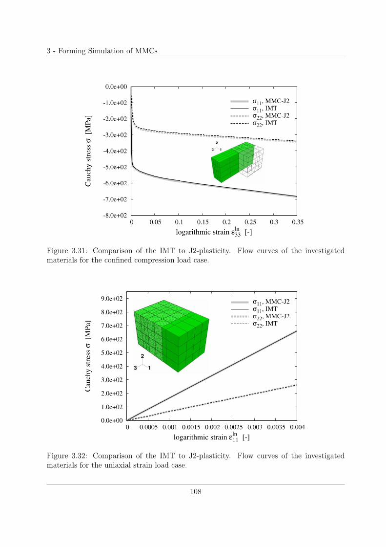
3 - Forming Simulation of MMCs
Figure 3.31: Comparison of the IMT to J2-plasticity. Flow curves of the investigatedmaterials for the confined compression load case.
Figure 3.32: Comparison of the IMT to J2-plasticity. Flow curves of the investigatedmaterials for the uniaxial strain load case.
108
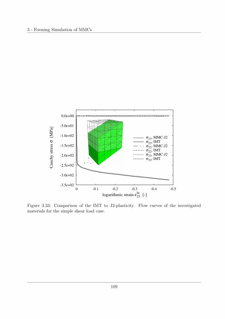
3 - Forming Simulation of MMCs
Figure 3.33: Comparison of the IMT to J2-plasticity. Flow curves of the investigatedmaterials for the simple shear load case.
109
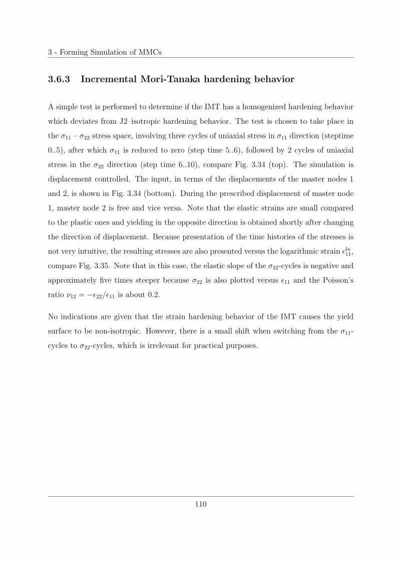
3 - Forming Simulation of MMCs
3.6.3 Incremental Mori-Tanaka hardening behavior
A simple test is performed to determine if the IMT has a homogenized hardening behavior
which deviates from J2–isotropic hardening behavior. The test is chosen to take place in
the σ11 – σ22 stress space, involving three cycles of uniaxial stress in σ11 direction (steptime
0..5), after which σ11 is reduced to zero (step time 5..6), followed by 2 cycles of uniaxial
stress in the σ22 direction (step time 6..10), compare Fig. 3.34 (top). The simulation is
displacement controlled. The input, in terms of the displacements of the master nodes 1
and 2, is shown in Fig. 3.34 (bottom). During the prescribed displacement of master node
1, master node 2 is free and vice versa. Note that the elastic strains are small compared
to the plastic ones and yielding in the opposite direction is obtained shortly after changing
the direction of displacement. Because presentation of the time histories of the stresses is
not very intuitive, the resulting stresses are also presented versus the logarithmic strain εln11,
compare Fig. 3.35. Note that in this case, the elastic slope of the σ22-cycles is negative and
approximately five times steeper because σ22 is also plotted versus ε11 and the Poisson’s
ratio ν12 = −ε22/ε11 is about 0.2.
No indications are given that the strain hardening behavior of the IMT causes the yield
surface to be non-isotropic. However, there is a small shift when switching from the σ11-
cycles to σ22-cycles, which is irrelevant for practical purposes.
110
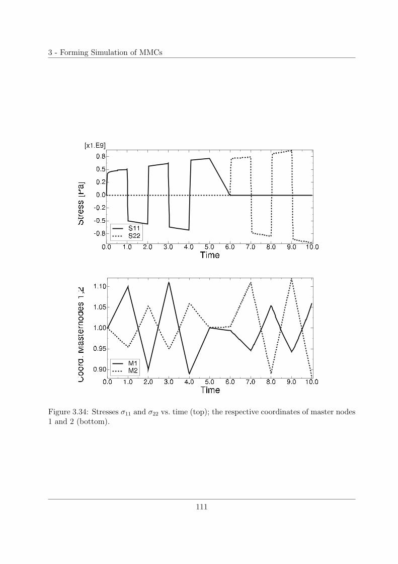
3 - Forming Simulation of MMCs
Figure 3.34: Stresses σ11 and σ22 vs. time (top); the respective coordinates of master nodes1 and 2 (bottom).
111
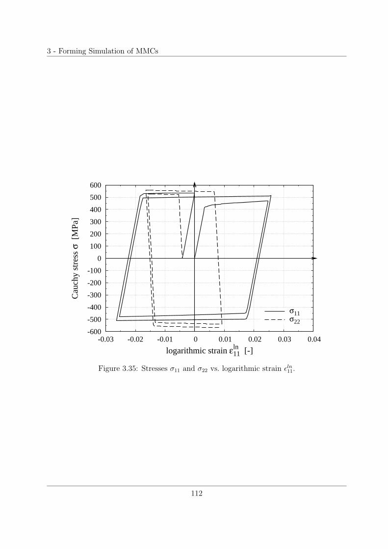
3 - Forming Simulation of MMCs
-600
-500
-400
-300
-200
-100
0
100
200
300
400
500
600
-0.03 -0.02 -0.01 0 0.01 0.02 0.03 0.04
Cau
chy
stre
ss σ
[M
Pa]
logarithmic strain εln11 [-]
σ11σ22
Figure 3.35: Stresses σ11 and σ22 vs. logarithmic strain εln11.
112
113
Chapter 4
Summary
Computational simulations of Metal Matrix Composites (MMCs) are performed with the
aim to improve computational predictions of the thermo-mechanical behavior in frictional
contact (Chapter 2) and of the elasto-plastic properties of MMCs undergoing finite strains
(Chapter 3). A hierarchical approach employing micromechanical methods within the
continuum mechanics framework is followed.
Chapter 2 deals with computational predictions of the tribological behavior of MMCs,
where the influence of particle volume fraction and clustering of particles is investigated
at different length scales. Finite Element simulations are performed employing periodic
unit cells with both homogeneous random and clustered distributions. Based on these
experiences, numerical simulations employing the Finite Element Method (FEM) of the
frictional behavior of a MMC material, including heat conduction in the steady state, are
performed. Experiments and analytical calculations jointly serve to determine unknown
process parameters by means of a simplified, homogenized model, whereas in the FEM
simulations, the inhomogeneous body is considered. The validity of the FE continuum
mechanics of materials approach utilizing unit cells is demonstrated in case of undercritical
conditions. However, limitations of the thermo-elastic FEM predictions are encountered

4 - Summary
and related to frictionally excited thermo-elastic instability. The stability limit is estimated
analytically using two different approaches from the literature and compared to the FEM
simulation findings. In view of these findings, the validity of thermo-elastic predictions
beyond the stable regime has to be seriously questioned. The stability limit needs to be
estimated in the first place, e.g. by the described analytical methods. Extrapolating from
results of linear elastic simulations to sliding speeds above the stability limit is not advised.
Chapter 3 is concerned with the computational simulation of a forming process of a par-
ticulate MMC component. A hierarchical concept is utilized within the framework of the
Finite Element Method to study a Gleeble-type experiment employing two micromechan-
ics of materials approaches. The analytical incremental Mori-Tanaka method, which has
been extended to account for finite strains, is employed to predict mesoscale responses and
approximations of microscale fields. The periodic microfield approach using unit cells is
utilized to predict the mesoscopic responses as well as the fluctuating microfields. It also
serves as a reference to assess the quality of the results of the analytical approach. The
advantages of the IMT are low computational costs in terms of speed and memory require-
ments, and the possibility to employ a micromechanical constitutive material law within
the FEM to a entire structure or component. Due to performance and capacity restrictions,
this is not possible with the PMA at the moment. When comparing the IMT results to
those of the PMA on the mesoscale, the former’s predictions are found to be excellent and
the assumptions made in the IMT’s formulations are shown to hold. Predictions on the
microscale are limited by the inherent mean field assumptions, though, so the PMA is still
the tool of choice on these length scales.
A comparison of the two constitutive material laws IMT and J2-plasticity is performed.
While for the given material, the difference in response is subtle, access to predictions on
the microscopic level is lost when only relying on the homogenized material. Furthermore,
a method to address mesoscopic strain concentration of periodic unit cells under certain
circumstances is presented.
114
115
Appendix A
Transformation of the deformation to
rotated coordinate systems, step by
step procedure
The presented approach is as follows. First the evolution of deformation, described by
the deformation gradient of the problem, is transformed into a rotated configuration. The
master node displacements are determined to perform the simulations in this rotated coor-
dinate system in order to solve the original problem. Homogenization is performed using
the reaction forces at the master nodes, compare Eq. (1.20), to provide the transition from
the micro to the mesoscopic level. The results, e.g. the Cauchy or the first Piola-Kirchhoff
stress tensors, are then transformed back to the original coordinate system.
The individual steps of the actual procedure are demonstrated by the example of simple
shear in the 23-plane.
1. The evolution of the deformation gradient, F (t), is prescribed in a master coordinate
system for the original, unrotated configuration using, e.g. Eq. (1.16).
2. Transform the deformation gradient to a rotated ′-coordinate system, F ′(t), in which

Appendix
the FEM analysis will be performed,
F ′ = R(α)F (t)RT(α) , (A.1)
with R(α) being the orthogonal (RT = R−1) transformation matrix of rank two
for rotation about the angle α. For example, R(α) for rotation about the 1-axis
(transforming the ’simple shear in the 23-plane’ problem) formally reads
R(α) =
⎛⎜⎜⎜⎜⎜⎝
1 0 0
0 cos(α) sin(α)
0 − sin(α) cos(α)
⎞⎟⎟⎟⎟⎟⎠ . (A.2)
3. From F ′(t), compute the evolution of the new master node coordinates, dx =
[d�x1, d�x2, d�x3], from the definition of the deformation gradient
dx = F ′ · dX . (A.3)
For the cubic unit cells employed, the column vectors of dx end up containing the
actual coordinates of the master nodes in the deformed configuration. From dx,
the displacements of the master nodes for performing the simulation in the rotated
configuration are computed by subtracting the identity matrix (the original position
vectors).
4. Run simulation in the rotated system by prescribing the nonlinear evolution of the
master node displacements, for example by employing amplitude curves.
5. Extract the reaction forces at the master nodes in the rotated configuration.
6. From the actual master node coordinates and periodicity vectors of the unit cells,
compute normal vectors, �ni, in the undeformed and deformed states, compare Eq. 1.19.
The normal vectors in the undeformed configuration follow from the vector product
of the initial periodicity vectors, where no displacements have occurred.
116
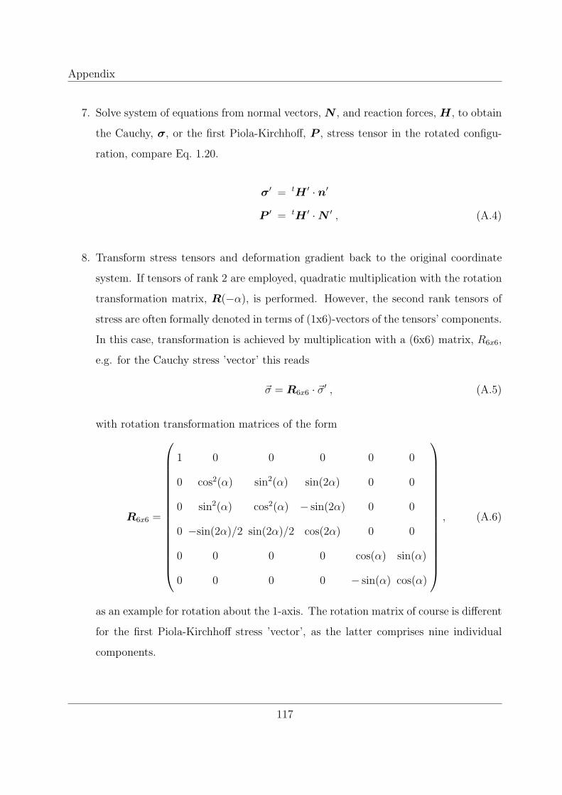
Appendix
7. Solve system of equations from normal vectors, N , and reaction forces, H , to obtain
the Cauchy, σ, or the first Piola-Kirchhoff, P , stress tensor in the rotated configu-
ration, compare Eq. 1.20.
σ′ = tH ′ · n′
P ′ = tH ′ · N ′ , (A.4)
8. Transform stress tensors and deformation gradient back to the original coordinate
system. If tensors of rank 2 are employed, quadratic multiplication with the rotation
transformation matrix, R(−α), is performed. However, the second rank tensors of
stress are often formally denoted in terms of (1x6)-vectors of the tensors’ components.
In this case, transformation is achieved by multiplication with a (6x6) matrix, R6x6,
e.g. for the Cauchy stress ’vector’ this reads
�σ = R6x6 · �σ′ , (A.5)
with rotation transformation matrices of the form
R6x6 =
⎛⎜⎜⎜⎜⎜⎜⎜⎜⎜⎜⎜⎜⎜⎜⎜⎜⎝
1 0 0 0 0 0
0 cos2(α) sin2(α) sin(2α) 0 0
0 sin2(α) cos2(α) − sin(2α) 0 0
0 −sin(2α)/2 sin(2α)/2 cos(2α) 0 0
0 0 0 0 cos(α) sin(α)
0 0 0 0 − sin(α) cos(α)
⎞⎟⎟⎟⎟⎟⎟⎟⎟⎟⎟⎟⎟⎟⎟⎟⎟⎠
, (A.6)
as an example for rotation about the 1-axis. The rotation matrix of course is different
for the first Piola-Kirchhoff stress ’vector’, as the latter comprises nine individual
components.
117
118
Bibliography
J.R. Barber. Thermoelastic Instabilities in the Sliding of Conforming Solids. Proc.Roy.Soc.,
pages 381–394, 1969.
Y. Benveniste. A New Approach to the Application of Mori-Tanaka’s Theory in Composite
Materials. Mechanics of Materials, 6(2):147–157, 1987.
B. Bhushan, editor. Modern Tribology Handbook, volume 1 - Principles of Tribology. CRC
Press, 2001.
D. B. Bogy. Two Edge-Bonded Elastic Wedges Of Different Materials And Wedge Angles
Under Surface Tractions. J. Appl. Mech., 38(2):377–386, 1971.
H.J. Bohm. A Short Introduction To Continuum Micromechanics. In Mechanics of Mi-
crostructured Materials, pages 1–40. CISM Courses and Lectures, Springer-Verlag, Vi-
enna, 2002.
H.J. Bohm, A. Eckschlager, and W. Han. Multi-Inclusion Unit Cell Models for Metal Ma-
trix Composites with Randomly Oriented Discontinuous Reinforcements. Computational
Material Science, 25(1-2):42–53, 2002.
H.J. Bohm, W. Han, and A. Eckschlager. Multi Inclusion Unit Cell Studies of Rein-
forcement Stresses and Particle Failure in Discontinuously Reinforced Ductile Matrix
Composites. Comput.Model.Engng.Sci, 5:2–20, 2004.
Bibliography
M. Bornert. Homogeneisation des milieux aleatoires: bornes et estimations. In Ho-
mogeneisation en mecanique des materiaux 1. Materiaux aleatoires elastiques et milieux
periodiques, pages 133–221, Paris, 2001. Editions Hermes.
M. Bornert, T. Bretheau, and P. Gilormini, editors. Homogeneisation en mechanique des
materiaux. 2. Comportements non lineaires et problemes ouverts. Hermes, Science, Paris,
2001.
M. Ciavarella and J.R. Barber. Stability of Thermoelastic Contact for a Rectangular Elastic
Block Sliding against a Rigid Wall. Eur. J. Mech. A/Solids, 24:371–376, 2005.
I. Doghri and A. Ouaar. Homogenization of Two-Phase Elasto-Plastic Composite Materials
and Structures. Int.J.Sol.Struct, 40 (7)(1):1681–1712, 2003.
T.A. Dow and R.A. Burton. Thermoelastic Instability of Sliding Contact in the Absence
of Wear. Wear, 19:315–328, 1972.
J.D. Eshelby. The Determination of the Elastic Field of an Ellisoidal Inclusion and Related
Problems. Proc.of the Royal Society London, A241:376–396, 1957.
G. Fichera. Boundary Value Problems of Elasticity with Unilateral Constraints. In Hand-
buch der Physik, volume a/2, pages 391–424. Springer, Berlin, 1972.
A.C. Gavazzi and D.C. Lagoudas. On the Numerical Evaluation of Eshelby’s Tensor and
its Application to Elastoplastic Fibrous Composites. Comput.Mech, 7:12–19, 1990.
C. Gonzalez and J. Llorca. A Self-consistent Approach to the Elasto-Plastic Behavior of
Two-phase Materials including Damage. J.Mech.Phys.Solids, 48:675–692, 2000.
R. Hill. Elastic Properties of Reinforced Solids: Some Theoretical Principles.
J.Mech.Phys.Sol, 11:357–372, 1963.
C.O Huber, M.H. Luxner, S. Kremmer, S. Nogales, H.J. Bohm, and H.E. Pettermann.
Forming Simulations of MMC Components by a Micromechanics Based Hierarchical
119
Bibliography
FEM Approach. In J. M. A. Cesar de Sa and A. D. Santos, editors, 9th International
Conference in Numerical Methods in Industrial Forming Processes (NUMIFORM07),
pages 1351–1357. American Institute of Physics, 2007.
K.L. Johnson. Contact Mechanics. Cambridge Univ. Pr., 1992.
N. Kikuchi and J.T. Oden. Contact Problems in Elasticity: A Study of Variational In-
equalities and Finite Element Methods. SIAM, Philadelphia, PA, 1988.
U. Landman, W.D. Luetke, and E.M. Ringer. Molecular Dynamics Simulations of Adhesive
Contact Formulation and Friction. In I.L. Singer and H.M. Pollock, editors, Fundamen-
tals of Friction: Macroscopic and Microscopic Processes, page 463. Kluwer Academic
Publishers, Dortrecht, 1993.
M. Luxner. Nichtlineare Homogenisierung von FEM Einheitszellenanalysen fur MMCs.
AAR-ILSB Report No.37, Institute of Lightweight Design and Structural Biomechanics,
Vienna University of Technology, 2007.
T. Mori and T. Tanaka. Average Stress in the Matrix and Average Elastic Energy of
Materials with Misfitting Inclusions. Acta Metall., 21(5):571–574, 1973.
D. H. Pahr. Linear and Non-linear Homogenization using FEM. Technical report, Institute
of Lightweight Design and Structural Biomechanics, Vienna University of Technology,
2004.
H. E. Pettermann, A. F. Plankensteiner, H. J. Bohm, and F. G. Rammerstorfer. A Thermo-
Elasto-Plastic Constitutive Law for Inhomogeneous Materials Based on an Incremental
Mori-Tanaka Approach. Computers and Structures, 71:197 – 214, 1999.
H.E. Pettermann. Derivation and Finite Element Implementation of Constitutive Mate-
rial Laws for Multiphase Composites Based on Mori-Tanaka Approaches. PhD thesis,
Institute of Lightweight Structures and Aerospace Engineering, Vienna University of
Technology, 1997. (also appeared as VDI Report 217/18, VDI-Verlag, Dusseldorf, Ger-
many, 1997).
120
Bibliography
H.E. Pettermann and S. Suresh. A Comprehensive Unit Cell Model for the Thermome-
chanical Response of 1-3 Piezoelectric Composites. International Journal of Solids and
Structures, 37:5447–5464, 2000.
H.E. Pettermann, H.J. Bohm, and F.G. Rammerstorfer. Some Direction Dependent Prop-
erties of Matrix-Inclusion Type Composites with Given Reinforcement Orientation Dis-
tributions. Composites, 28B(3):1–24, 1997.
H.E. Pettermann, C.O. Huber, M.H. Luxner, S. Nogales, and H.J. Bohm. Finite Elastic-
Plastic Deformation of MMC Components – Multiscale Mean Field and Unit Cell Sim-
ulations. In Volume of Abstracts of the 35th Solid Mechanics Conference, SolMech2006,
Krakow, Poland, 2006.
O. Pierard and I. Doghri. A Study of Various Estimates of the Macroscopic Tan-
gent Operator in the Incremental Homogenization of Elasto-plastic Composites.
Int.J.Mult.Comp.Eng., 4(4):521–543, 2006.
C. Poletti. Hot Deformation and Properties of PRTi alloys. PhD thesis, Vienna University
of Technology, Vienna, 2005.
C. Poletti, W. Marketz, and H.P. Degischer. Hot Formability of a Particle Reinforced
Ti-Alloy. Ti-2003 Science and Technology, pages 2531–2538, 2003.
C. Poletti, A. Merstallinger, Th. Schubert, W. Marketz, and H.P. Degischer. Wear and
Friction Coefficients of Particle Reinforced Ti-Alloys. Mat.-wiss. u. Werkstofftech., 35
(10):741 – 749, 2004.
F.G. Rammerstorfer and H.J. Bohm. Lecture Notes Composite Engineering. Institute of
Lightweight Structures and Structural Biomechanics, Vienna University of Technology.
Vienna, Austria, 2004.
D.A. Rigney and J.P. Hirth. Plastic Deformation and Sliding Friction of Metals. Wear,
53:345–370, 1979.
121
Bibliography
C. Schuecker. Mechanism based modeling of damage and failure in fiber reinforced polymer
laminates. PhD thesis, Vienna University of Technology, 2005.
J. Segurado, A. Merstallinger, and H.E. Pettermann. Numerical Simulations in Tribology
– A Micro-mechanics of Materials Approach. In Proc.of the WTC2001. The Austrian
Tribology Society, Austria, 2001.
Simulia Inc. ABAQUS/Standard Manual. Providence, RI, USA, v6.4 edition, 2004.
S. Suresh, A. Mortensen, and A. Needleman, editors. Fundamentals of Metal-Matrix Com-
posites. Butterworth-Heinemann, Stoneham, MA, USA, 1993.
G.P. Tandon and G.J. Weng. A Theory of Particle-Reinforced Plasticity. J.Appl.Mech.,
55:126–135, 1988.
H. Uetz and J. Fohl. Wear as an Energy Transformation Process. Wear, 49:253–264, 1978.
G.J. Weng. The Theoretical Connection between Mori-Tanaka Theory and the Hashin-
Shtrikman-Walpole Bounds. Int.J.Engng.Sci., 28:1111–1120, 1990.
C. Zweben. Comprehensive Composite Materials, volume 3 - Metal Matrix Composites.
Cambridge University Press, UK, 2000.
122


