Two Dimensional Viewing
Dr. S.M. MalaekAssistant: M. Younesi

Two Dimensional Viewing
Basic Interactive Programming

Basic Interactive Programming
User controls contents, structure, and appearance of objects and their displayed images via rapid visual feedback.
Model
Model: a pattern, plan, representation, or description designed to show the structure or working of an object, system, or concept.

Modeling
Modeling is the process of creating, storing and manipulating a model of an object or a system.
ModelingIn Modeling, we often use a geometric model
i.e.. A description of an object that provides a numerical description of its shape, size and various other properties.
Dimensions of the object are usually given in units appropriate to the object:
meters for a shipkilometres for a country
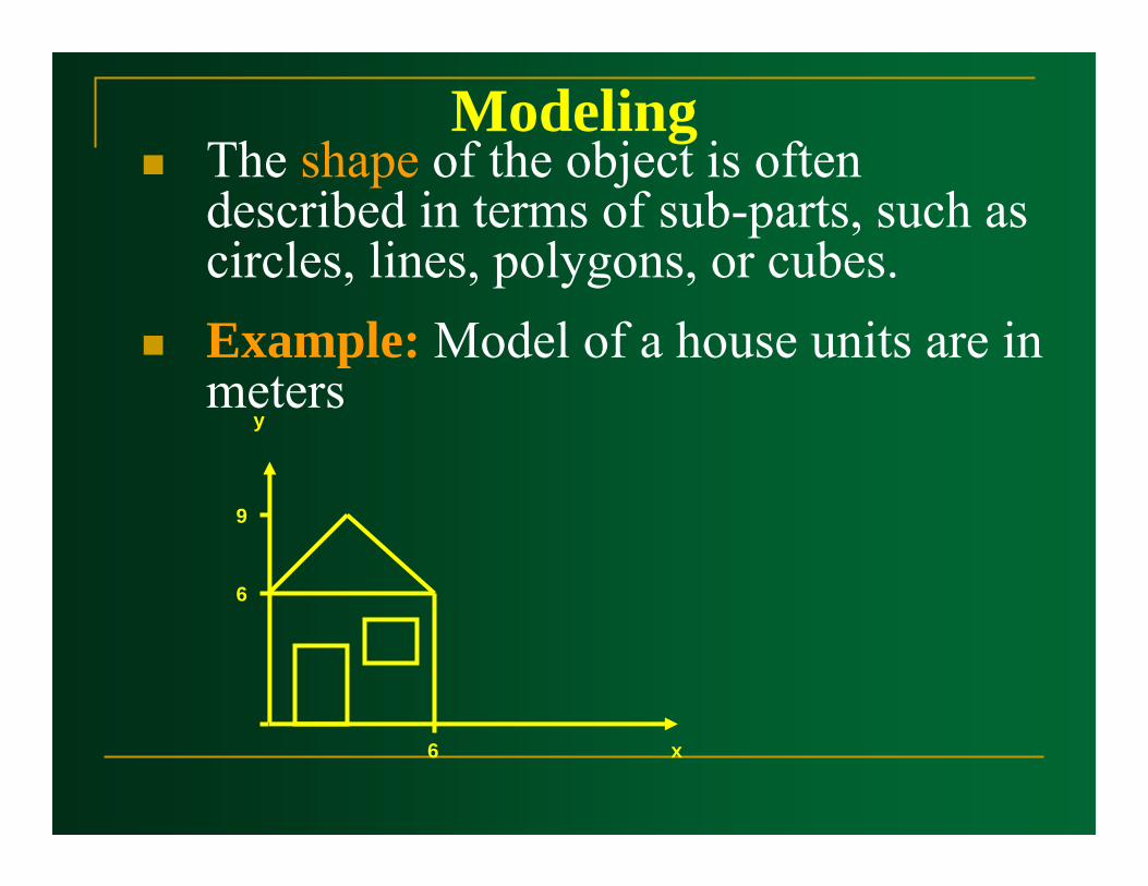
ModelingThe shape of the object is often described in terms of sub-parts, such as circles, lines, polygons, or cubes.Example: Model of a house units are in meters
6
9
6
y
x

6
9
y
x
Instances of this object may then be placed in various positions in a scene, or world, scaled to different sizes, rotated, or deformed.
Each house is created with instances of the same model, but with different parameters.
Instances of Objects

2D Viewing
2D Viewing
Viewing is the process of drawing a view of a
model on a 2-dimensional display.
2D ViewingThe geometric description of the object or scene provided by the model, is converted into a set of graphical primitives, which are displayed where desired on a 2D display.
The same abstract model may be viewed in many different ways:
e.g. faraway, near, looking down, looking up
Real World CoordinatesIt is logical to use dimensions which are appropriate to the object e.g.
meters for buildingsnanometers or microns for molecules, cells, atomslight years for astronomy
The objects are described with respect to their actual physical size in the real world, and then mappedmapped onto screenscreen co-ordinates.
It is therefore possible to view an object at various sizes by zooming in and out, without actually having to change the model.
2D ViewingHow muchHow much of the model should be drawn?
WhereWhere should it appear on the display?
HowHow do we convert Real-world coordinates into screen co-ordinates?
We could have a model of a whole room, full of objectssuch as chairs, tablets and students. We may want to view the whole room in one go, or zoom in on one single object in the room.We may want to display the object or scene on the full screen, or we may only want to display it on a portion of the screen.
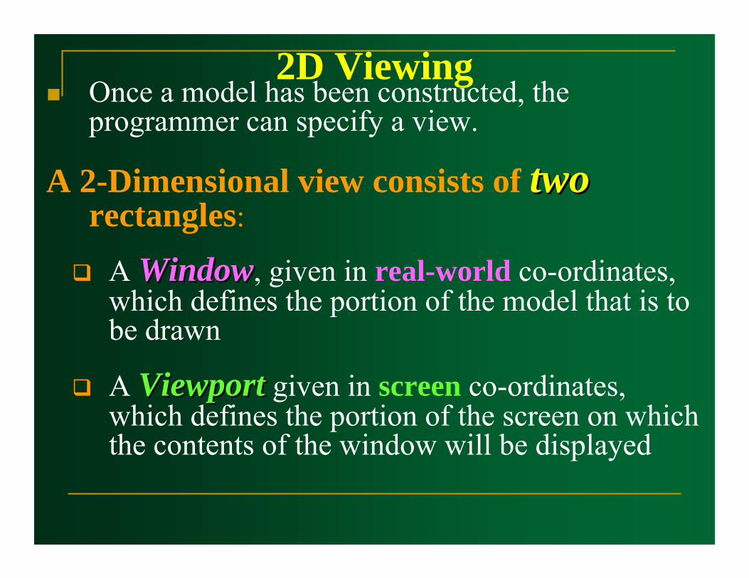
2D ViewingOnce a model has been constructed, the programmer can specify a view.
A 2-Dimensional view consists of twotworectangles:
A WindowWindow, given in real-world co-ordinates, which defines the portion of the model that is to be drawn
A ViewportViewport given in screen co-ordinates, which defines the portion of the screen on which the contents of the window will be displayed
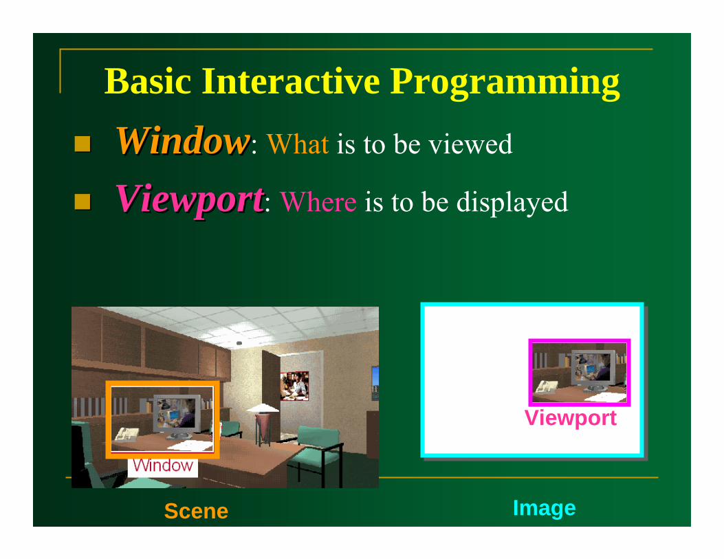
Basic Interactive ProgrammingWindowWindow: What is to be viewed
ViewportViewport: Where is to be displayed
Scene Image
Viewport
Coordinate Representations
Coordinate RepresentationsGeneral graphics packages are designed to be used with Cartesian coordinate specifications.
Several different Cartesian reference frame are used to construct and display a scene.

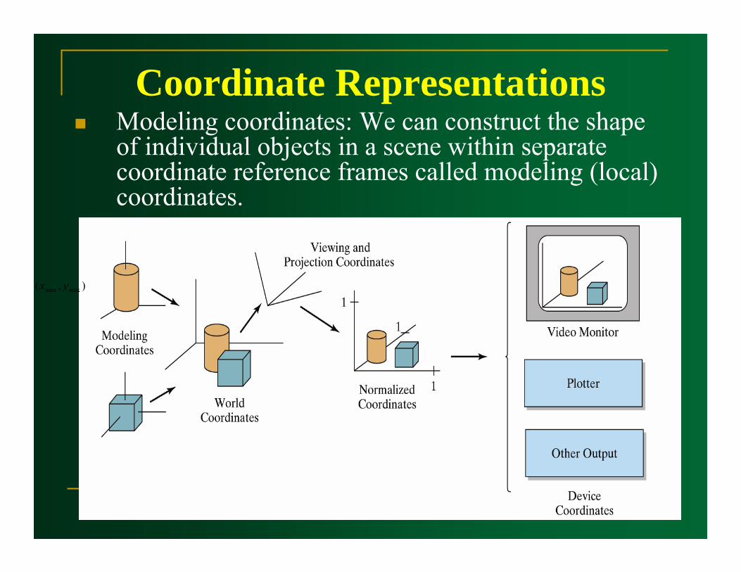
Coordinate RepresentationsModeling coordinates: We can construct the shape of individual objects in a scene within separate coordinate reference frames called modeling (local) coordinates.
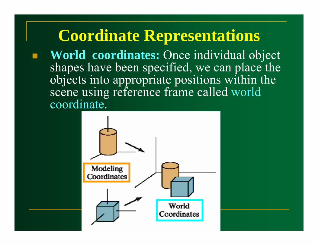
Coordinate RepresentationsWorld coordinates: Once individual object shapes have been specified, we can place the objects into appropriate positions within the scene using reference frame called world coordinate.
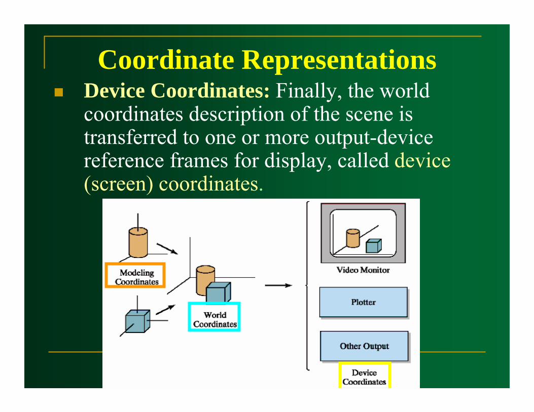
Coordinate RepresentationsDevice Coordinates: Finally, the world coordinates description of the scene is transferred to one or more output-device reference frames for display, called device (screen) coordinates.
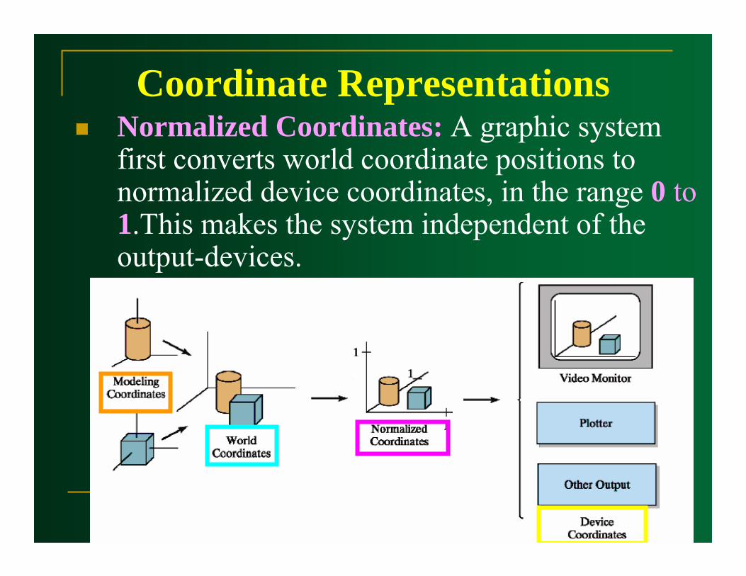
Coordinate RepresentationsNormalized Coordinates: A graphic system first converts world coordinate positions to normalized device coordinates, in the range 0 to1.This makes the system independent of the output-devices.
Coordinate RepresentationsModeling coordinates: We can construct the shape of individual objects in a scene within separate coordinate reference frames called modeling (local) coordinates.
),( maxmax yx
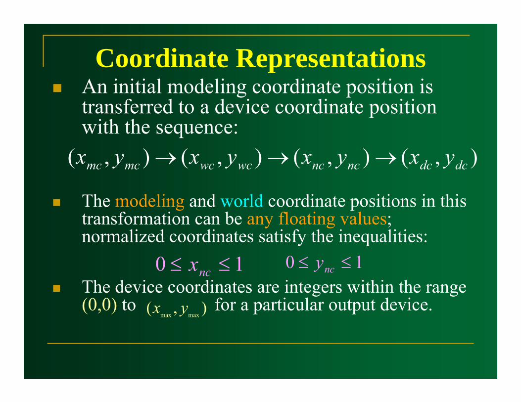
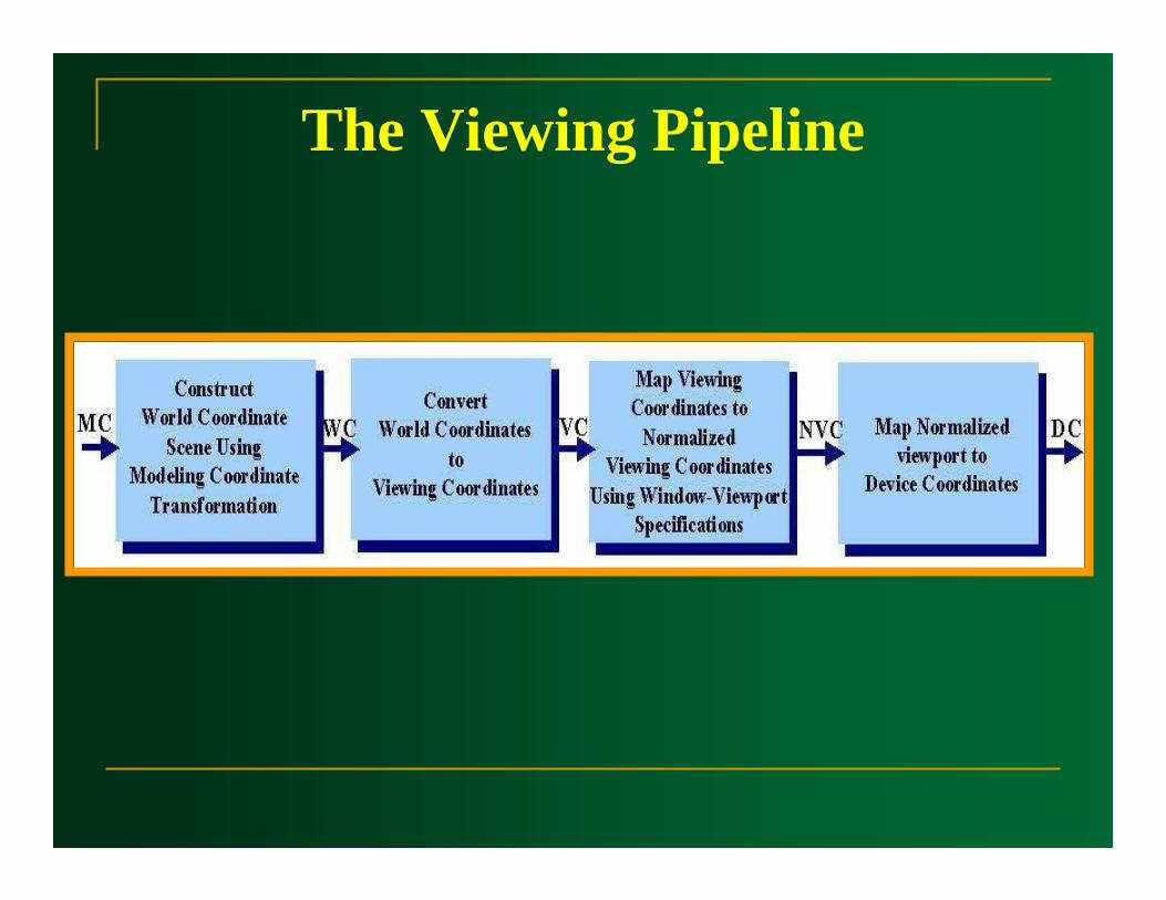
Coordinate RepresentationsAn initial modeling coordinate position is transferred to a device coordinate position with the sequence:
The modeling and world coordinate positions in this transformation can be any floating values; normalized coordinates satisfy the inequalities:
The device coordinates are integers within the range (0,0) to for a particular output device.
),(),(),(),( dcdcncncwcwcmcmc yxyxyxyx →→→
10 ≤≤ ncx 10 ≤≤ ncy
),( maxmax yx
The Viewing Pipeline
The Viewing PipelineA world coordinate area selected for display is called window.An area on a display device to which a window is mapped a viewport.
Windows and viewports are rectangular in standard position.
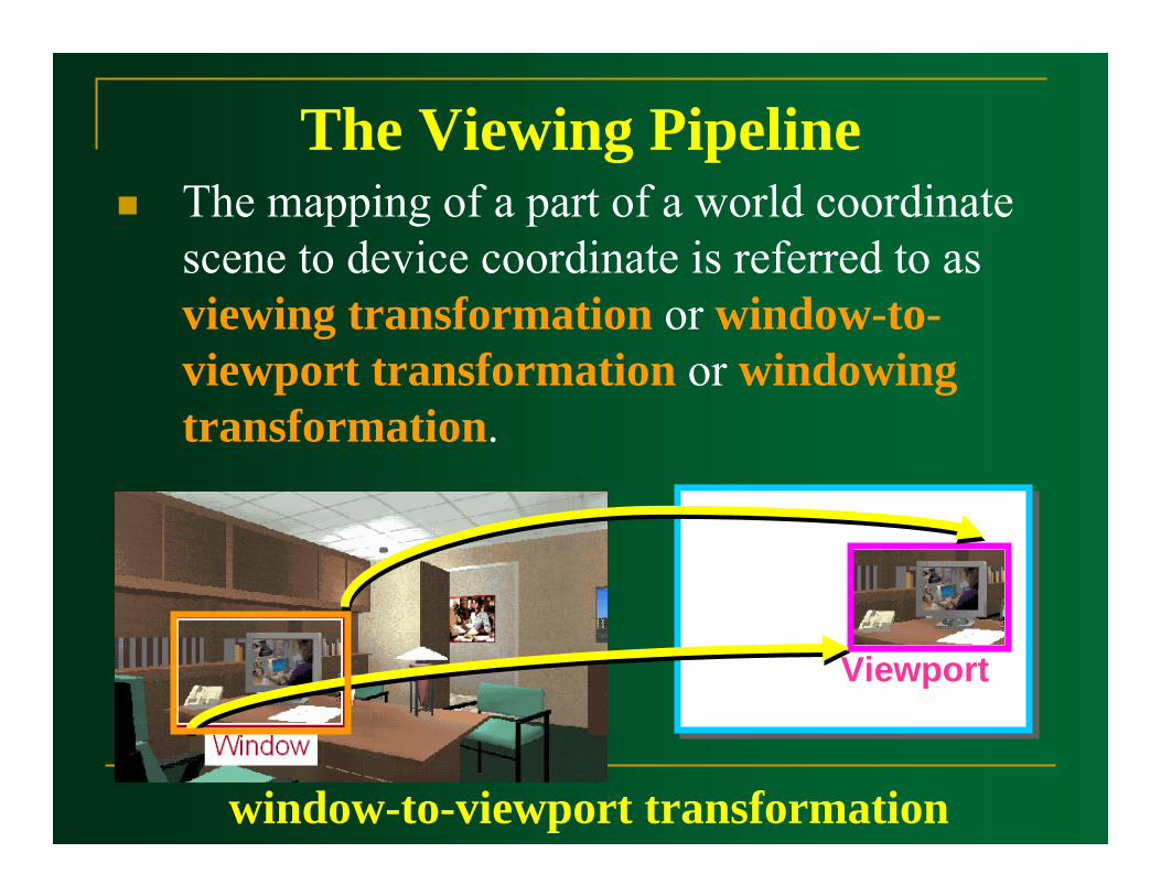
The Viewing PipelineThe mapping of a part of a world coordinate scene to device coordinate is referred to as viewing transformation or window-to-viewport transformation or windowing transformation.
Viewport
window-to-viewport transformation
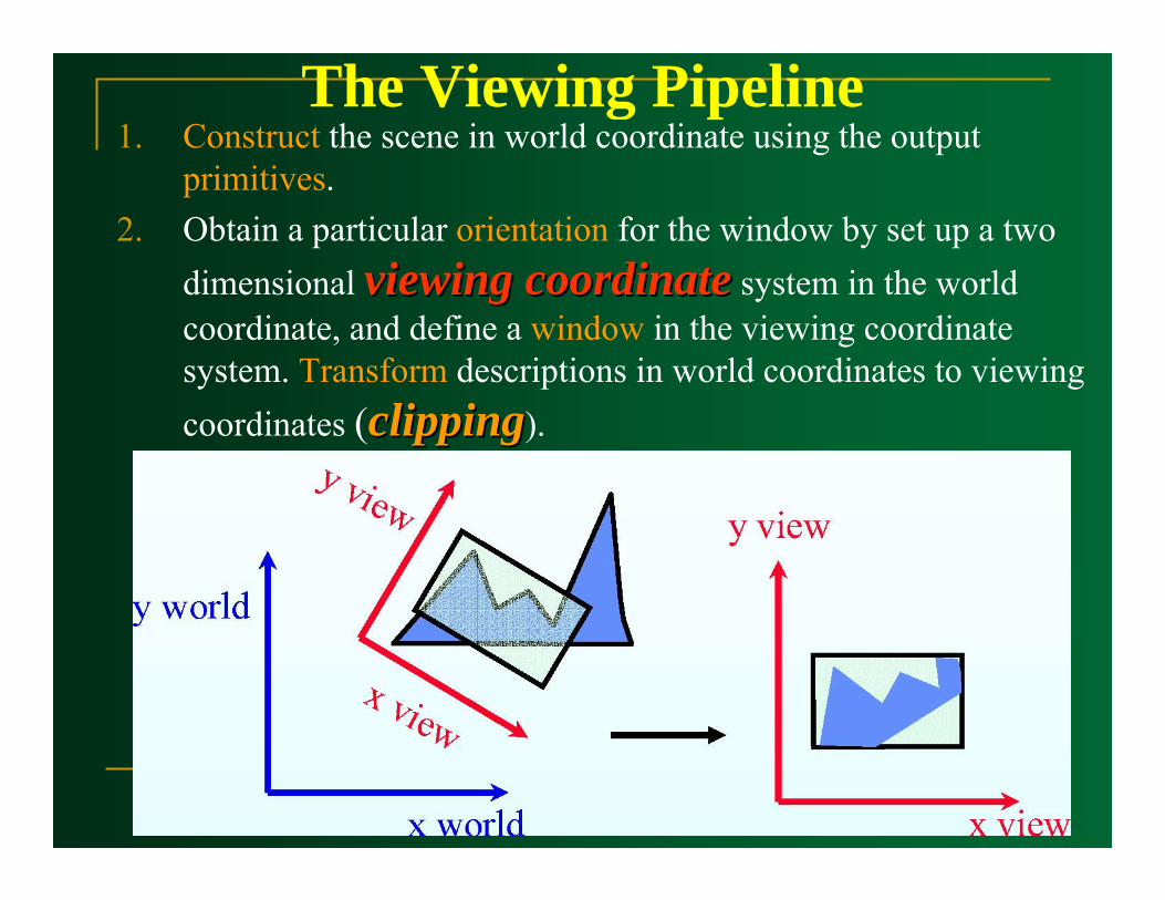
The Viewing Pipeline1. Construct the scene in world coordinate using the output
primitives.2. Obtain a particular orientation for the window by set up a two
dimensional viewing coordinateviewing coordinate system in the world coordinate, and define a window in the viewing coordinate system. Transform descriptions in world coordinates to viewing coordinates (clippingclipping).

The Viewing Pipeline3. Define a viewport in normalized coordinate, and map the
viewing coordinate description of the scene to normalizedcoordinate
4. (All parts lie outside the viewport are clippedclipped), and contents of the viewport are transferred to device coordinates.
Viewing Coordinate Normalized Coordinate Device Coordinate
1
1
The Viewing Pipeline
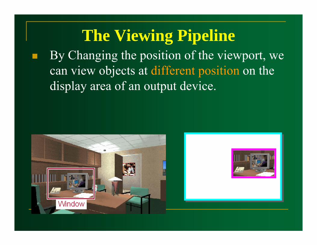
The Viewing PipelineBy Changing the position of the viewport, we can view objects at different position on the display area of an output device.
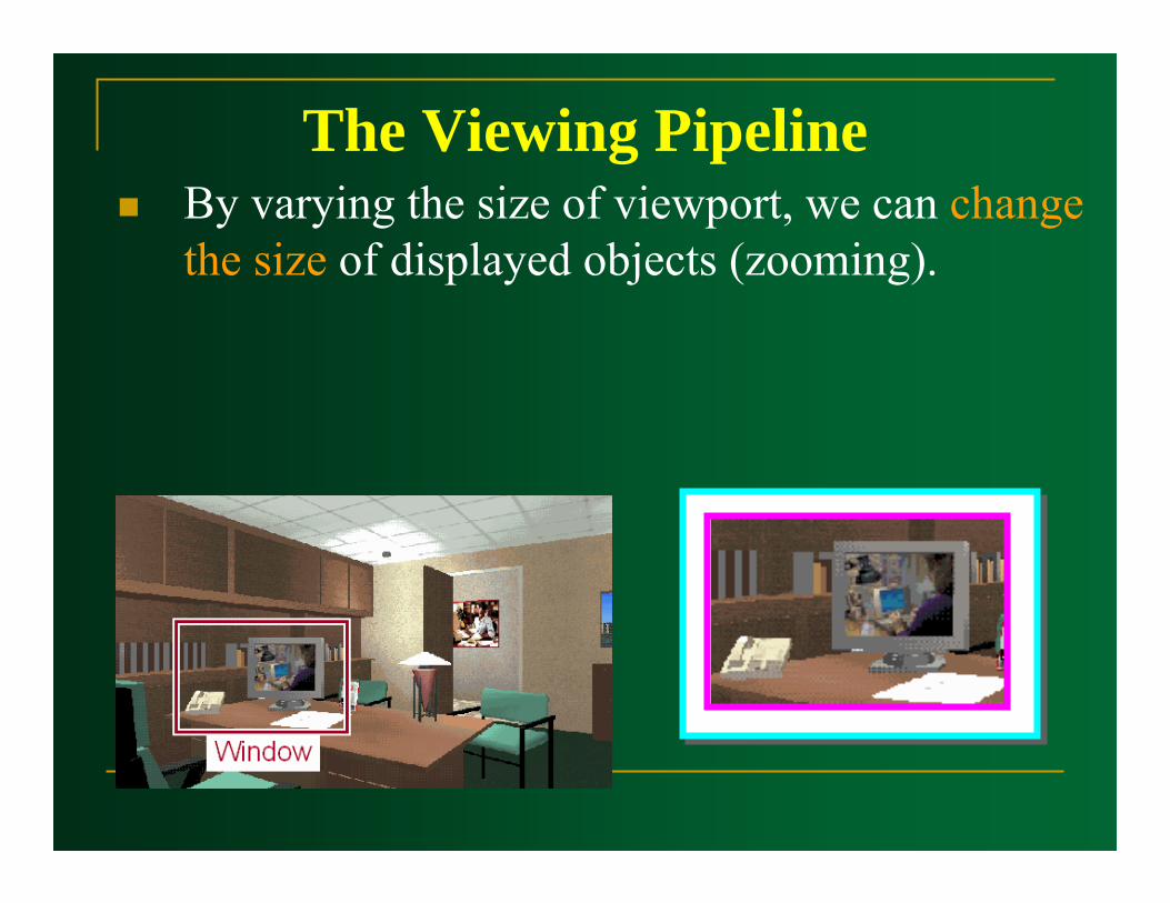
The Viewing PipelineBy varying the size of viewport, we can change the size of displayed objects (zooming).

2D Geometric Transformations
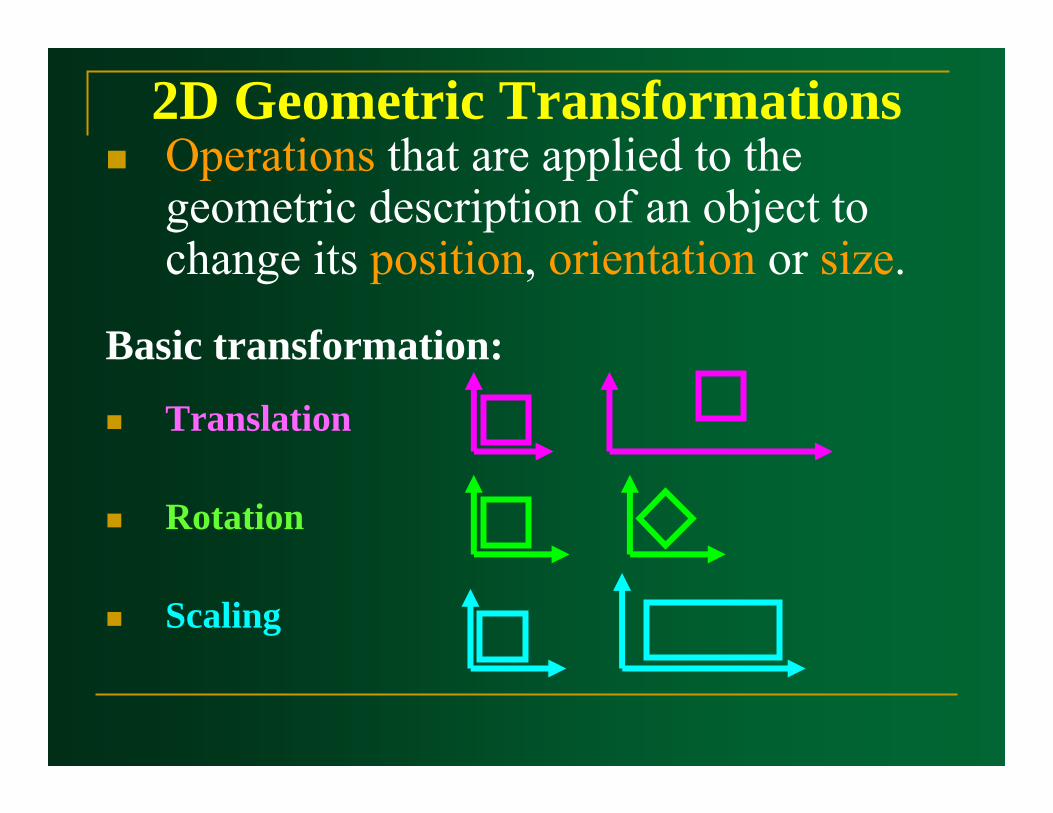
2D Geometric TransformationsOperations that are applied to the geometric description of an object to change its position, orientation or size.
Basic transformation:
Translation
Rotation
Scaling
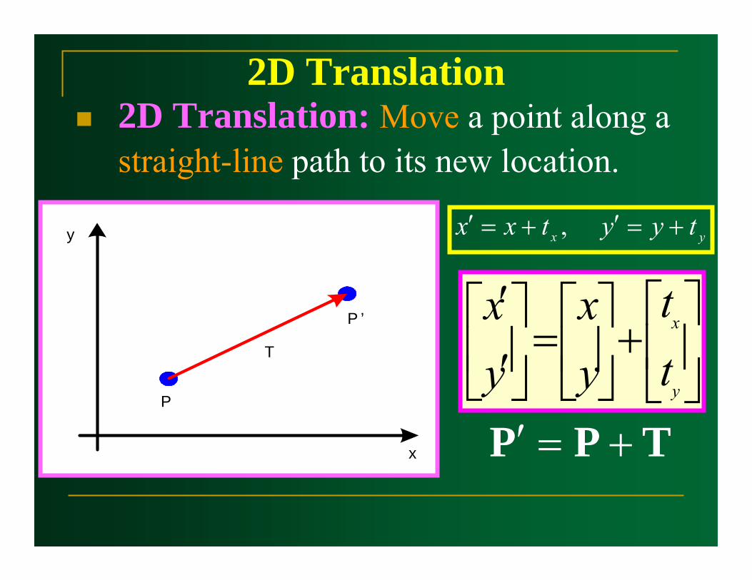
2D Translation2D Translation: Move a point along a straight-line path to its new location.
P
P ’
T
x
y yx tyytxx +=′+=′ ,
⎥⎦
⎤⎢⎣
⎡+⎥⎦
⎤⎢⎣
⎡=⎥⎦
⎤⎢⎣
⎡′′
y
x
tt
yx
yx
TPP +=′
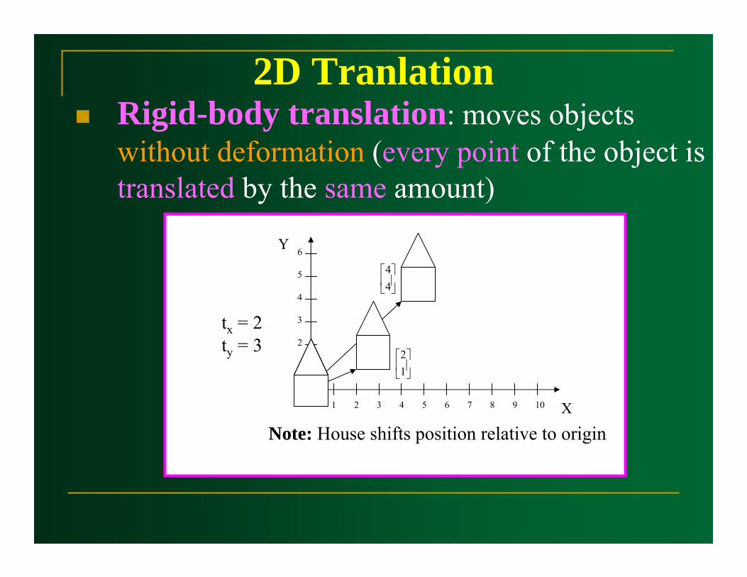
2D TranlationRigid-body translation: moves objects without deformation (every point of the object is translated by the same amount)
Note: House shifts position relative to origin
tx = 2ty = 3
Y
X0
1
1
2
2
3 4 5 6 7 8 9 10
3
4
5
6
⎥⎦
⎤⎢⎣
⎡12
⎥⎦
⎤⎢⎣
⎡44
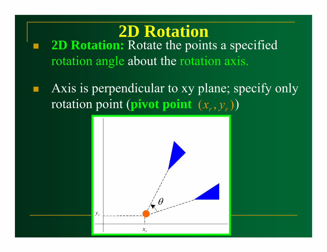
2D Rotation2D Rotation: Rotate the points a specified rotation angle about the rotation axis.
Axis is perpendicular to xy plane; specify only rotation point (pivot point ) ),( rr yx
rx
ry
θ

2D RotationSimplify: rotate around origin: 0,0 == rr yx
θ
φ
),( yx
)','( yx
rr
θcosφsinθsinφcos)θφsin(θsinφsinθcosφcos)θφcos(
rrryrrrx
+=+=′−=+=′
φsin,φcos ryrx ==
θcosθsinθsinθcos
yxyyxx
+=′−=′
PRP ⋅=′
⎥⎦
⎤⎢⎣
⎡ −=
θcosθsinθsinθcos
R
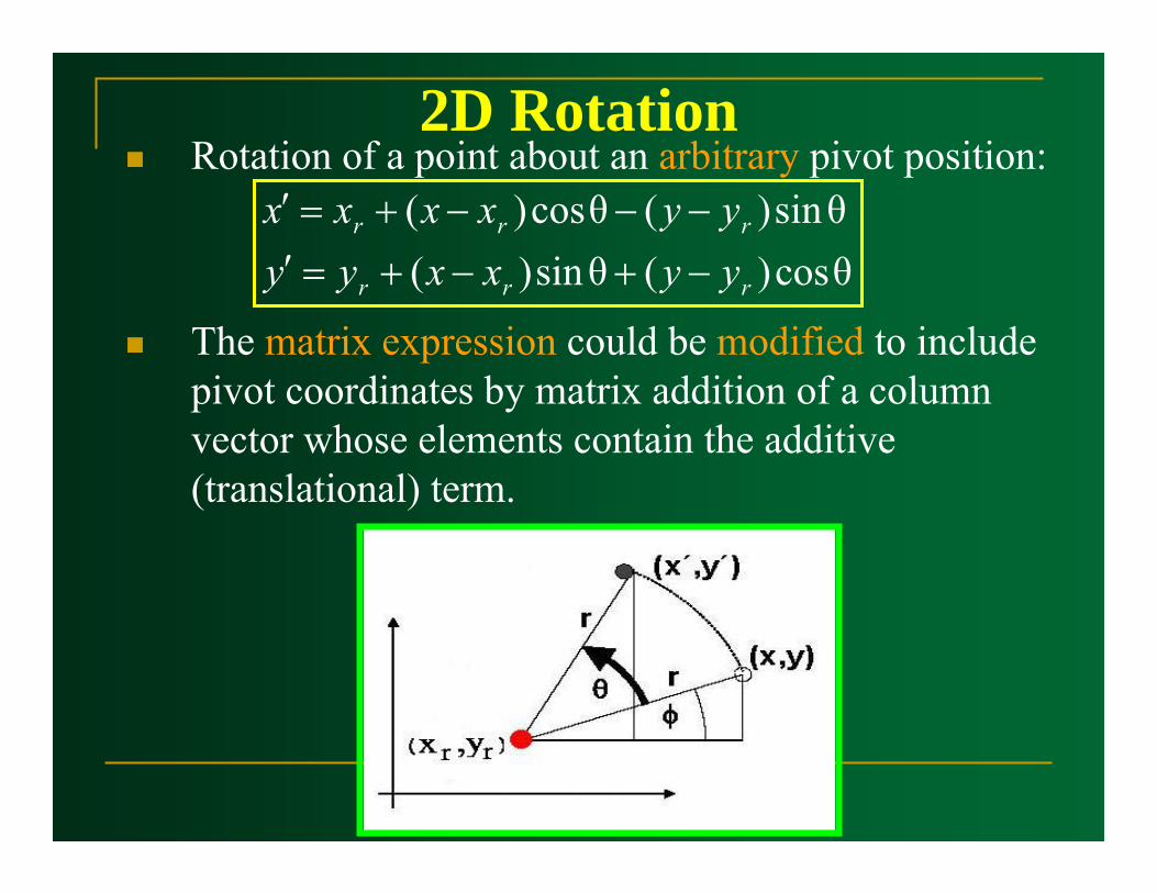
2D RotationRotation of a point about an arbitrary pivot position:
The matrix expression could be modified to include pivot coordinates by matrix addition of a column vector whose elements contain the additive (translational) term.
θcos)(θsin)(θsin)(θcos)(
rrr
rrr
yyxxyyyyxxxx
−+−+=′−−−+=′
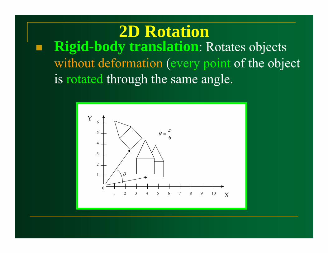
2D RotationRigid-body translation: Rotates objects without deformation (every point of the object is rotated through the same angle.
6πθ =
Y
X0
1
1
2
2
3 4 5 6 7 8 9 10
3
4
5
6
θ
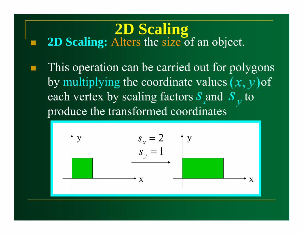
2D Scaling2D Scaling: Alters the size of an object.
This operation can be carried out for polygons by multiplying the coordinate values of each vertex by scaling factors and to produce the transformed coordinates
),( yxxs ys
x
y
x
y2=xs1=ys
2D Scaling
x
y
x
y2=xs1=ys
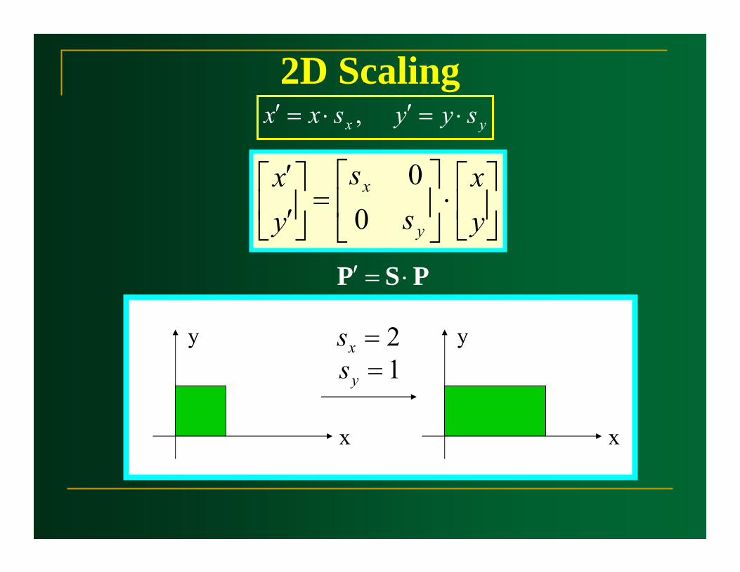
yx syysxx ⋅=′⋅=′ ,
⎥⎦
⎤⎢⎣
⎡⋅⎥⎦
⎤⎢⎣
⎡=⎥
⎦
⎤⎢⎣
⎡′′
yx
ss
yx
y
x
00
PSP ⋅=′
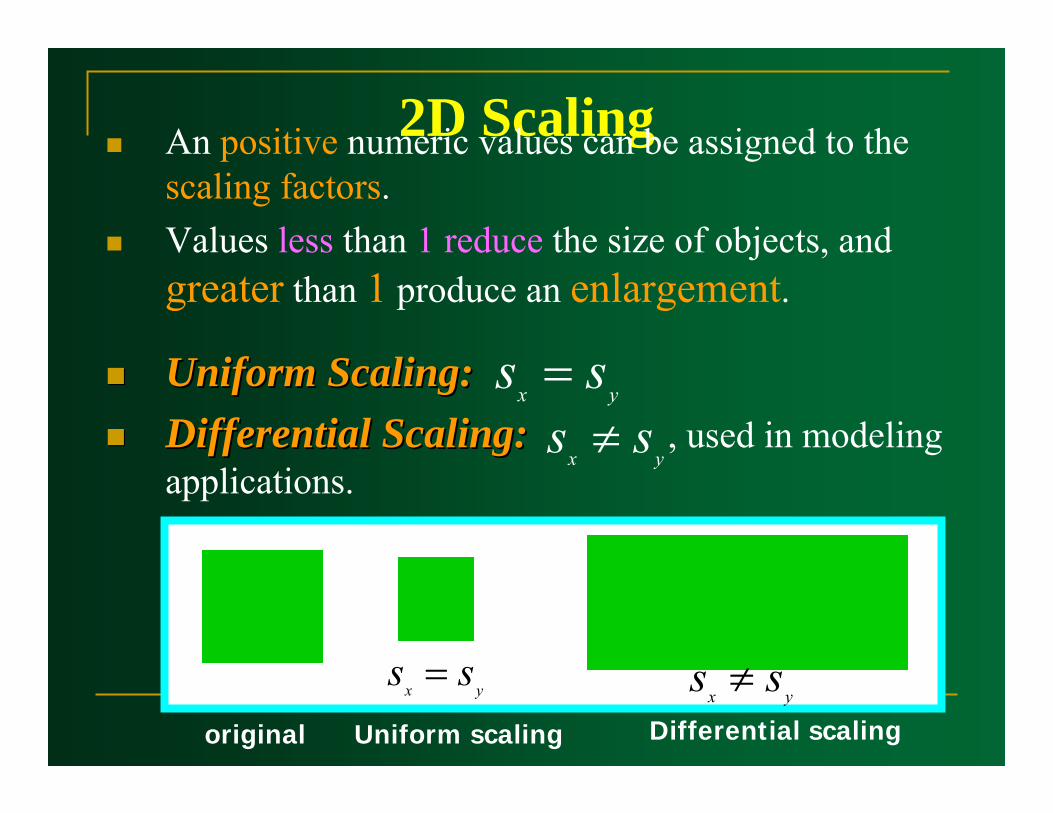
2D ScalingAn positive numeric values can be assigned to the scaling factors.Values less than 1 reduce the size of objects, and greater than 1 produce an enlargement.
Uniform Scaling:Uniform Scaling:Differential Scaling:Differential Scaling: , used in modeling applications.
yx ss =yx ss ≠
original Uniform scaling Differential scaling
yx ss =yx ss ≠
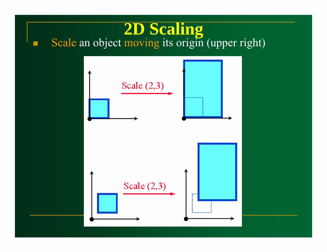
2D ScalingScale an object moving its origin (upper right)

2D ScalingWe can control the location of a scaled object by choosing a position, called fixes pointFixes point can be chosen as one of the vertices, the object centroid, or any other position
),( ff yx
xff sxxxx ⋅−+= )('
yff syyyy ⋅−+= )('
)1('xfx sxsxx −+⋅=
)1('yfy sysyy −+⋅=
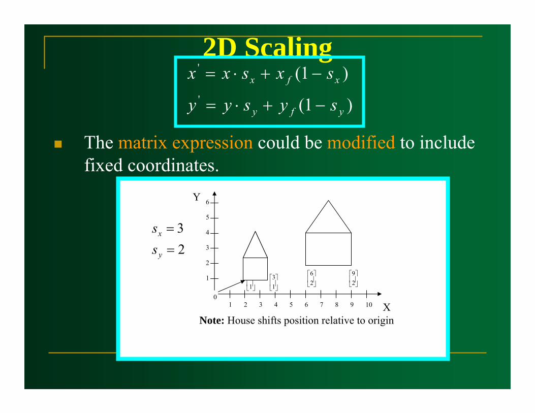
2D Scaling
The matrix expression could be modified to include fixed coordinates.
Note: House shifts position relative to origin
Y
X0
1
1
2
2
3 4 5 6 7 8 9 10
3
4
5
6
⎥⎦
⎤⎢⎣
⎡12
⎥⎦
⎤⎢⎣
⎡13 ⎥
⎦
⎤⎢⎣
⎡26
⎥⎦
⎤⎢⎣
⎡29
23
==
y
x
ss
)1('xfx sxsxx −+⋅=
)1('yfy sysyy −+⋅=
Matrix Representations And
Homogeneous Coordinates

Matrix RepresentationsIn Modeling, we perform sequences of geometric transformation: translation, rotation, and scaling to model components into their proper positions.
HowHow the matrix representations can be reformulated so that transformation sequences can be efficiently processed??
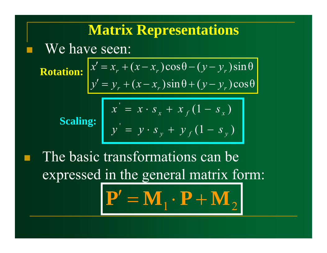
Matrix RepresentationsWe have seen:
)1('xfx sxsxx −+⋅=
)1('yfy sysyy −+⋅=
θcos)(θsin)(θsin)(θcos)(
rrr
rrr
yyxxyyyyxxxx
−+−+=′−−−+=′
The basic transformations can be expressed in the general matrix form:
21 MPMP +⋅=′
Rotation:
Scaling:
Matrix Representations
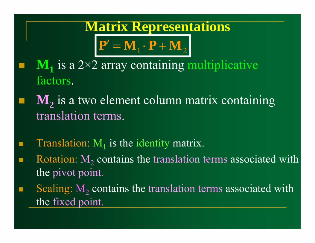
M1 is a 2×2 array containing multiplicative factors.M2 is a two element column matrix containing translation terms.
Translation: M1 is the identity matrix.Rotation: M2 contains the translation terms associated with the pivot point.Scaling: M2 contains the translation terms associated with the fixed point.
21 MPMP +⋅=′
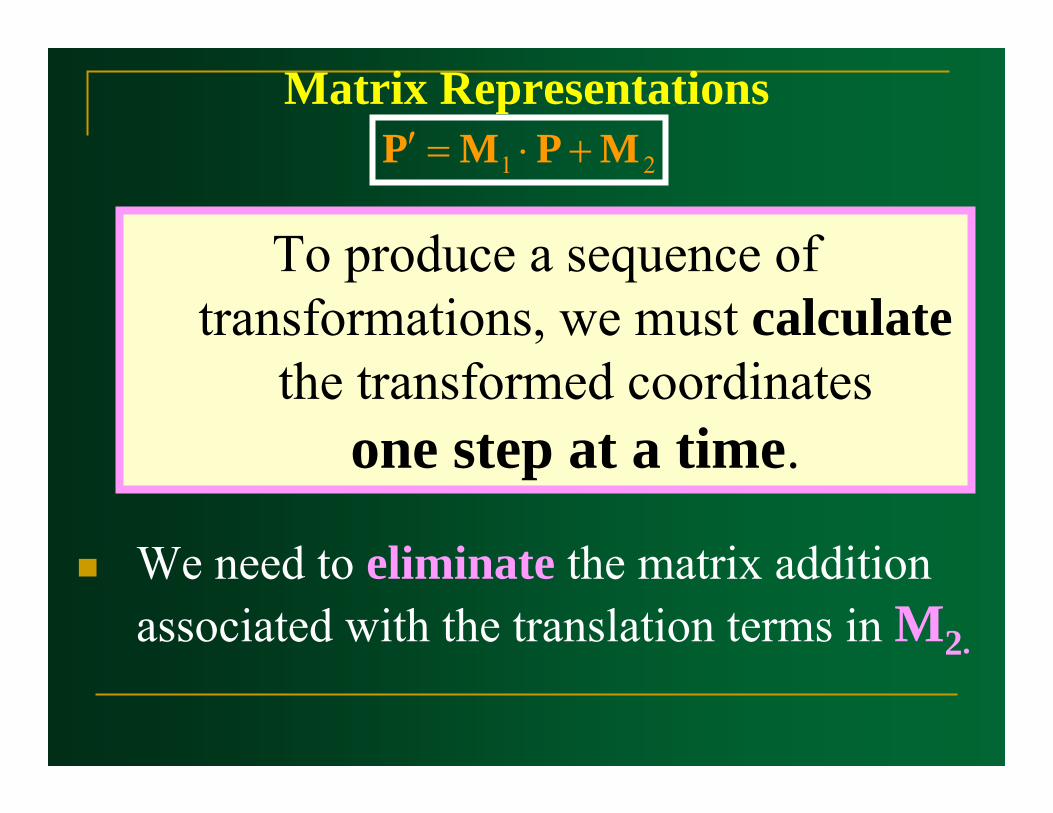
Matrix Representations
To produce a sequence of transformations, we must calculate
the transformed coordinates one step at a time.
21 MPMP +⋅=′
We need to eliminate the matrix addition associated with the translation terms in M2.
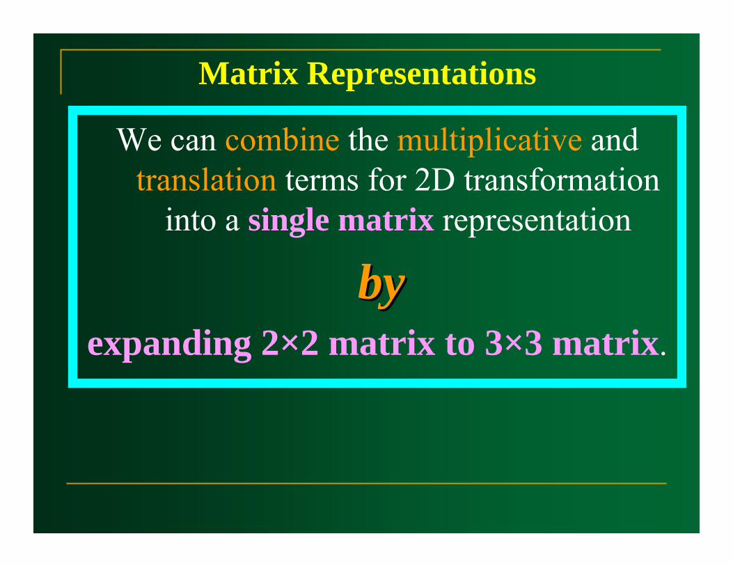
Matrix Representations
We can combine the multiplicative and translation terms for 2D transformation
into a single matrix representation
bybyexpanding 2×2 matrix to 3×3 matrix.
Matrix Representationsand
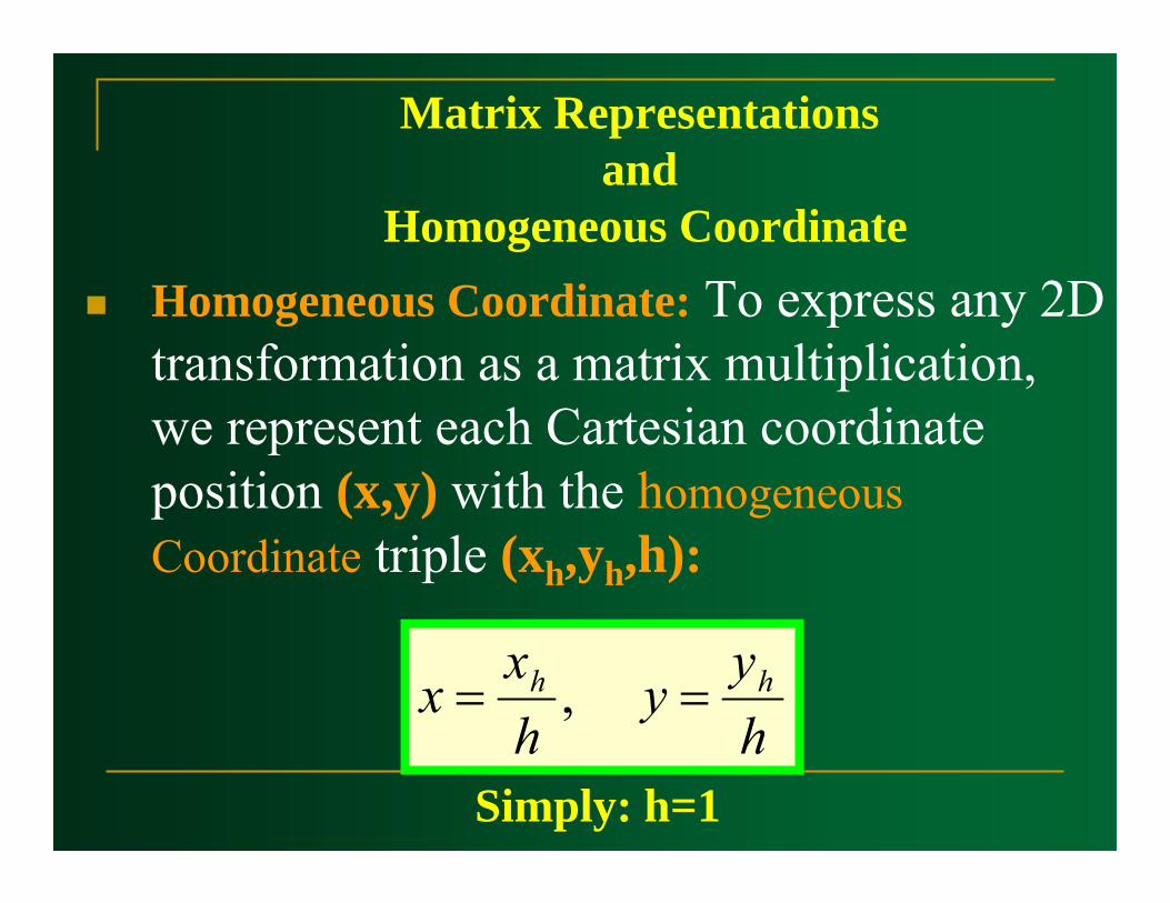
Homogeneous CoordinateHomogeneous Coordinate: To express any 2D transformation as a matrix multiplication, we represent each Cartesian coordinate position (x,y) with the homogeneousCoordinate triple (xh,yh,h):
hyy
hxx hh == ,
Simply: h=1
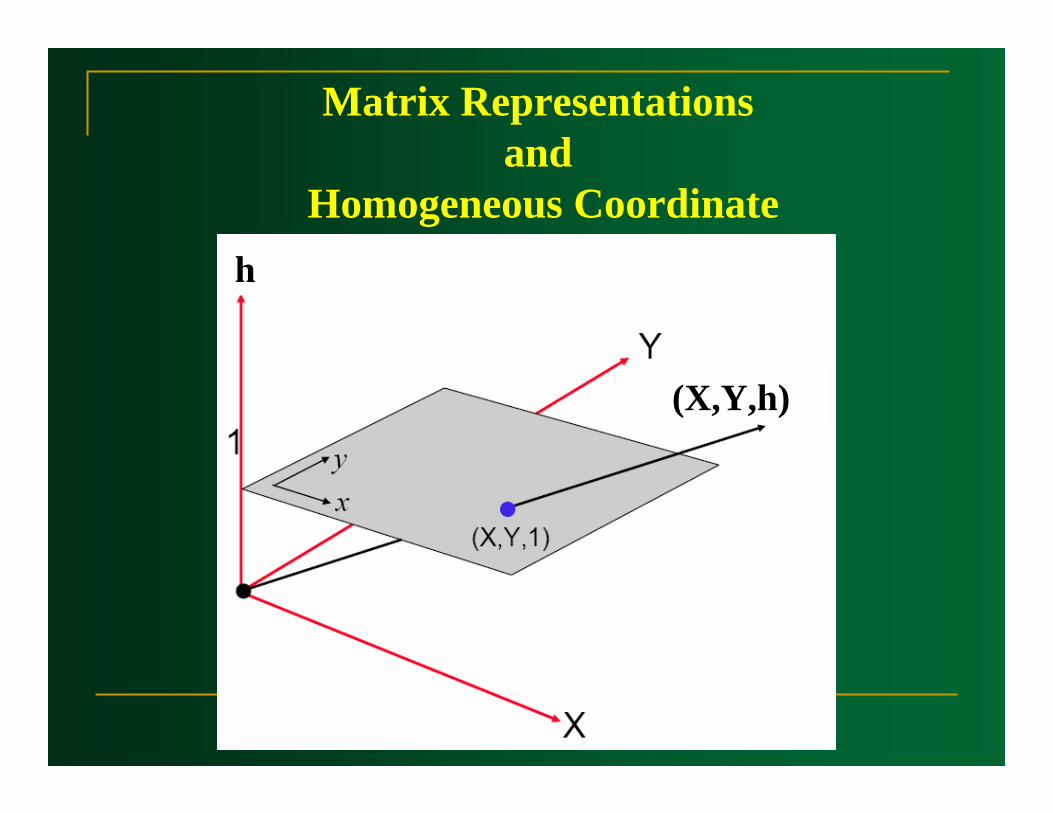
Matrix Representationsand
Homogeneous Coordinate
(X,Y,h)
h
Matrix Representationsand
Homogeneous Coordinate
Expressing position in homogeneous Coordinates,
(x,y,1) allows us to represent all geometric transformation as
matrix multiplication
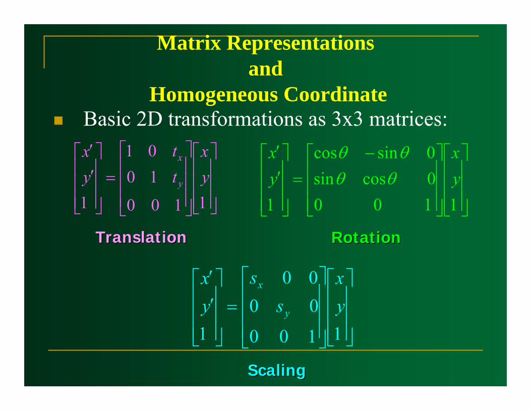
Matrix Representationsand
Homogeneous CoordinateBasic 2D transformations as 3x3 matrices:
⎥⎥⎥
⎦
⎤
⎢⎢⎢
⎣
⎡
⎥⎥⎥
⎦
⎤
⎢⎢⎢
⎣
⎡
=⎥⎥⎥
⎦
⎤
⎢⎢⎢
⎣
⎡′′
1100
1001
1yx
tt
yx
y
x
⎥⎥⎥
⎦
⎤
⎢⎢⎢
⎣
⎡
⎥⎥⎥
⎦
⎤
⎢⎢⎢
⎣
⎡
=⎥⎥⎥
⎦
⎤
⎢⎢⎢
⎣
⎡′′
1100
0000
1yx
ss
yx
y
x
⎥⎥⎥
⎦
⎤
⎢⎢⎢
⎣
⎡
⎥⎥⎥
⎦
⎤
⎢⎢⎢
⎣
⎡ −=
⎥⎥⎥
⎦
⎤
⎢⎢⎢
⎣
⎡′′
11000cossin0sincos
1yx
yx
θθθθ
TranslationTranslation RotationRotation
ScalingScaling
Composite Transformation

Composite TransformationCombined transformations
By matrix multiplication
Efficiency with pre-multiplication)))((( pSRTp ×××=′ pSRTp ×××=′ )(
⎥⎥⎥
⎦
⎤
⎢⎢⎢
⎣
⎡⋅⎟⎟⎟
⎠
⎞
⎜⎜⎜
⎝
⎛
⎥⎥⎥
⎦
⎤
⎢⎢⎢
⎣
⎡⋅⎥⎥⎥
⎦
⎤
⎢⎢⎢
⎣
⎡⋅⎥⎥⎥
⎦
⎤
⎢⎢⎢
⎣
⎡=
⎥⎥⎥
⎦
⎤
⎢⎢⎢
⎣
⎡
′′′
wyx
s
s
θθθ -θ
tt
wyx
y
x
y
x
1000000
1000cossin0sincos
1001001
p′ )( yx t,tT )(θR )( yx s,sS p=

General Pivot PointRotation

General Pivot Point Rotation
⎥⎥⎥
⎦
⎤
⎢⎢⎢
⎣
⎡θ−θ−θθθ+θ−θ−θ
=⎥⎥⎥
⎦
⎤
⎢⎢⎢
⎣
⎡−−
⋅⎥⎥⎥
⎦
⎤
⎢⎢⎢
⎣
⎡θθθ−θ
⋅⎥⎥⎥
⎦
⎤
⎢⎢⎢
⎣
⎡
100sin)cos1(cossinsin)cos1(sincos
1001001
1000cossin0sincos
1001001
rr
rr
r
r
r
r
xyyx
yx
yx
( ) ( ) ( ) ( )θ=−−⋅θ⋅ ,,,, rrrrrr yxyxyx RTRT
Translation Rotation Translation
(xr,yr) (xr,yr) (xr,yr)(xr,yr)

General Fixed PointScaling
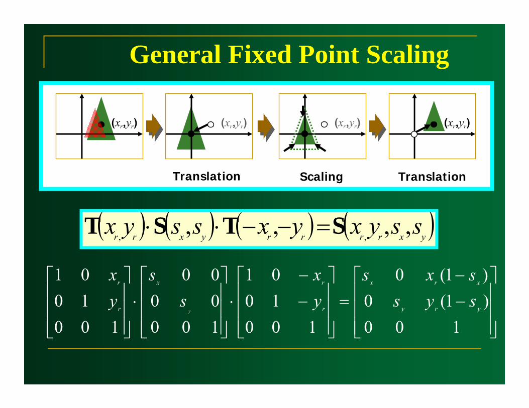
General Fixed Point Scaling
⎥⎥⎥
⎦
⎤
⎢⎢⎢
⎣
⎡−−
=⎥⎥⎥
⎦
⎤
⎢⎢⎢
⎣
⎡−−
⋅⎥⎥⎥
⎦
⎤
⎢⎢⎢
⎣
⎡⋅
⎥⎥⎥
⎦
⎤
⎢⎢⎢
⎣
⎡
100)1(0)1(0
1001001
1000000
1001001
yry
xrx
r
rx
r
r
syssxs
yx
ss
yx
y
( ) ( ) ( ) ( )yxrrrryxrr ssyxyxssyx ,,,, ,, STST =−−⋅⋅
Translation Scaling Translation
(xr,yr) (xr,yr) (xr,yr)(xr,yr)

General Scaling Direction
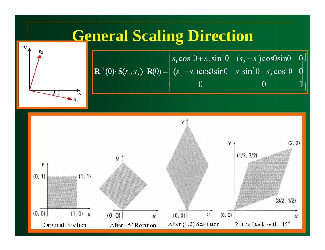
General Scaling Direction
⎥⎥⎥
⎦
⎤
⎢⎢⎢
⎣
⎡
+−−+
=⋅⋅−
1000θcosθsinθsinθcos)(0θsinθcos)(θsinθcos
)θ(),()θ( 22
2112
122
22
1
211 ssss
ssssss RSR

Reflection
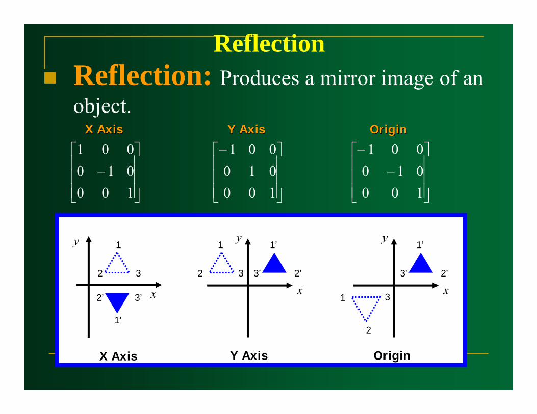
ReflectionReflection: Produces a mirror image of an object.
⎥⎥⎥
⎦
⎤
⎢⎢⎢
⎣
⎡−
100010001
⎥⎥⎥
⎦
⎤
⎢⎢⎢
⎣
⎡−
100010001
⎥⎥⎥
⎦
⎤
⎢⎢⎢
⎣
⎡−
−
100010001
x
y 1
32
1’
3’2’
1
32
1’
3’ 2’
x
y
3
1’
3’ 2’
1
2
x
y
X AxisX Axis Y AxisY Axis OriginOrigin
X AxisX Axis Y AxisY Axis OriginOrigin
Reflection
⎥⎥⎥
⎦
⎤
⎢⎢⎢
⎣
⎡
100001010 y=x
x
y
x
y
x
y 1
32
1’
3’2’ x
y
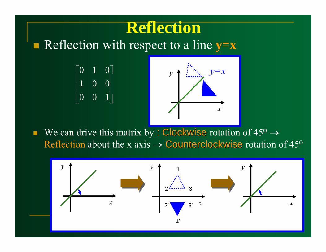
Reflection with respect to a line y=x
We can drive this matrix by : Clockwise: Clockwise rotation of 45º →Reflection about the x axis → CounterclockwiseCounterclockwise rotation of 45º
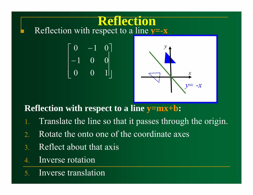
ReflectionReflection with respect to a line y=-x
y= -x
x
y
⎥⎥⎥
⎦
⎤
⎢⎢⎢
⎣
⎡−
−
100001010
Reflection with respect to a line y=mx+b:1. Translate the line so that it passes through the origin.2. Rotate the onto one of the coordinate axes3. Reflect about that axis4. Inverse rotation5. Inverse translation

Shear
ShearShear: A transformation that distorts the shape of an object such that transformed shape appears as if the object were composed of internal layers that had been caused to slide over each other is called a shear.
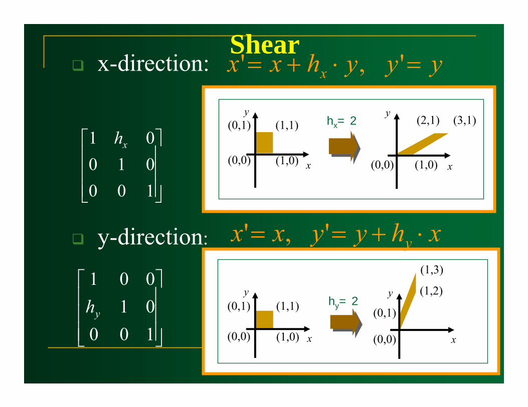
Shearx-direction: yyyhxx x =⋅+= ' ,'
(0,0) (1,0)
(1,1)(0,1) hx= 2
x
y(3,1)
(0,0) (1,0)
(2,1)
x
y
(0,0) (1,0)
(1,1)(0,1)
(0,0)
(0,1)
(1,3)
(1,2)hy= 2
x
y
x
y
⎥⎥⎥
⎦
⎤
⎢⎢⎢
⎣
⎡
10001001 xh
⎥⎥⎥
⎦
⎤
⎢⎢⎢
⎣
⎡
10001001
yh
y-direction: xhyyxx y ⋅+== ' ,'
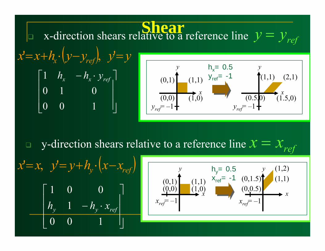
Shearx-direction shears relative to a reference line
( ) yyyyhxx refx =−⋅+= ' ,'
y-direction shears relative to a reference line
(0,0) (1,0)
(1,1)(0,1)
hx= 0.5yref= -1
x
y
yref= –1 yref= –1(0.5,0) (1.5,0)
(2,1)(1,1)
x
y
refyy =
(0,0) (1,0)(1,1)(0,1)
hy= 0.5xref= -1
x
y
(0,0.5)(1,1)(1,2)
(0,1.5)
x
y
xref= –1xref= –1
⎥⎥⎥
⎦
⎤
⎢⎢⎢
⎣
⎡ ⋅−
100010
1 refxx yhh
refxx =( )refy xxhyyxx −⋅+== ' ,'
⎥⎥⎥
⎦
⎤
⎢⎢⎢
⎣
⎡⋅−
1001
001
refyy xhh
Transformations Between
Coordinates Systems

Transformations Between Coordinates Systems
It is often requires the transformation of object description from one coordinate system to another.
How do we transform between two How do we transform between two Cartesian coordinate systems?Cartesian coordinate systems?
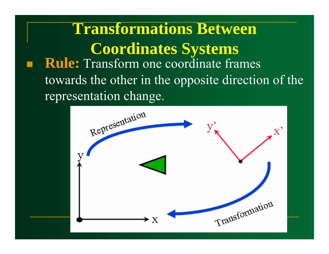
Transformations Between Coordinates Systems
Rule: Transform one coordinate frames towards the other in the opposite direction of the representation change.

Transformations Between Coordinates Systems
Two Steps:1. Translate so that the origin (x0,y0) of the x´y´
system is moved to the origin of the xy system.
2. Rotate the x´ axis onto the x axis.
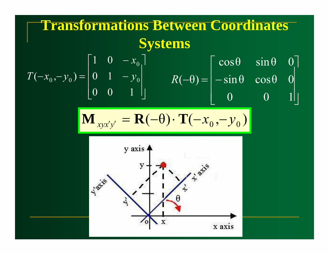
Transformations Between Coordinates Systems
⎥⎥⎥
⎦
⎤
⎢⎢⎢
⎣
⎡−−
=−−100
1001
),( 0
0
00 yx
yxT
⎥⎥⎥
⎦
⎤
⎢⎢⎢
⎣
⎡−=−
1000θcosθsin0θsinθcos
)θ(R
),()θ( 00 yxyxxy −−⋅−=′′ TRM

Transformations Between Coordinates Systems
Alternative Method:Assume x´=(ux,,uy) and y´=(vx,vy) in the (x,y) coordinate systems:
⎥⎥⎥
⎦
⎤
⎢⎢⎢
⎣
⎡−−
⋅⎥⎥⎥
⎦
⎤
⎢⎢⎢
⎣
⎡=
1001001
10000
0
0
yx
vvuu
M yx
yx
PP M=′
TRM ⋅=

Transformations Between Coordinates Systems
Example:
If V=(-1,0) then the xx´́ axis is in the positivepositivedirection yy and the rotation transformation matrix is:
⎥⎥⎥
⎦
⎤
⎢⎢⎢
⎣
⎡−=
100001010
R
Transformations Between Coordinates Systems
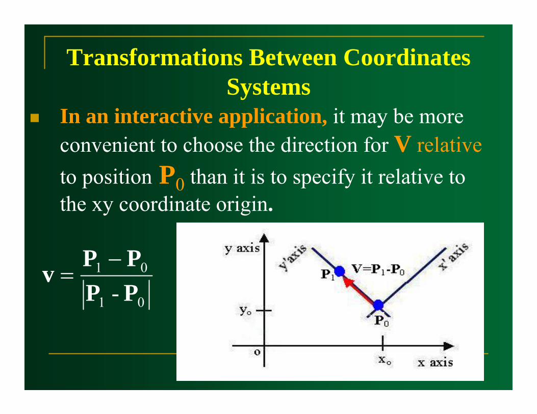
In an interactive application, it may be more convenient to choose the direction for V relative to position P0 than it is to specify it relative to the xy coordinate origin.
01
01
- PPPPv −
=
Viewing Coordinate Reference Frame
Viewing Coordinate Reference Frame
This coordinate system provides the reference frame for specifying the world coordinate window.
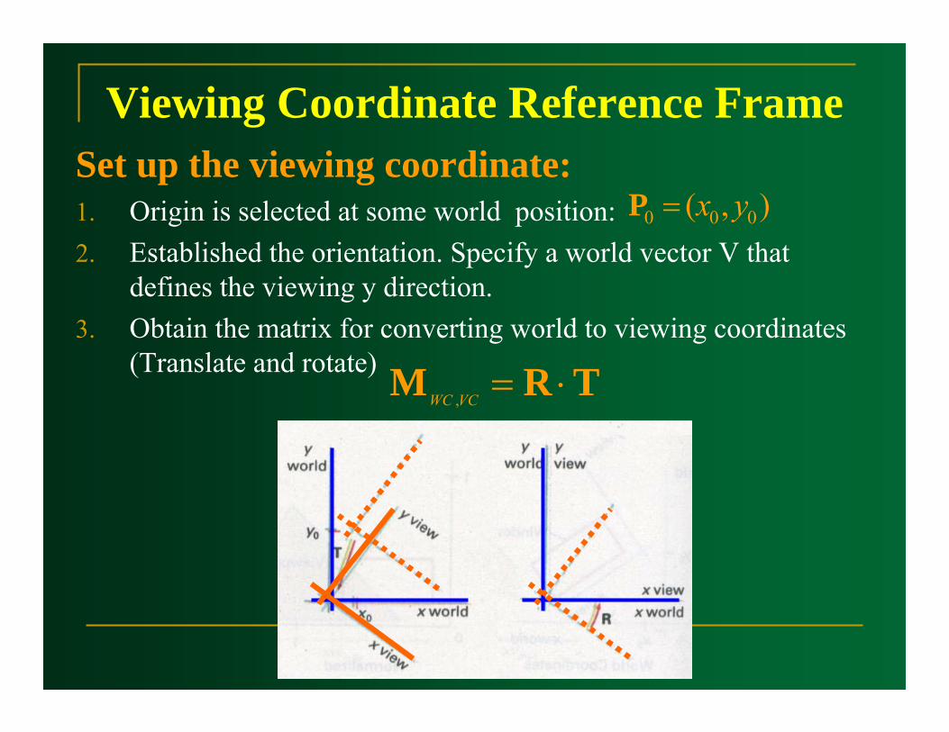
Viewing Coordinate Reference FrameSet up the viewing coordinate:1. Origin is selected at some world position: 2. Established the orientation. Specify a world vector V that
defines the viewing y direction.3. Obtain the matrix for converting world to viewing coordinates
(Translate and rotate)
),( 000 yx=P
TRM ⋅=VCWC ,

Window to ViewportCoordinate
Transformation

Window to Viewport Coordinate Transformation
Select the viewport in normalized coordinate, and then object description transferred to normalized device coordinate.To maintain the same relative placement in the viewport as in the window:
minmax
min
minmax
min
minmax
min
minmax
min
ywywywyw
yvyvyvyv
xwxwxwxw
xvxvxvxv
−−
=−
−−
−=
−−

Window to Viewport Coordinate Transformation
1. Perform a scaling transformation that scales the window area to the size of the viewport.
2. Translate the scaled window area to the position of the vieport.
minmax
min
minmax
min
minmax
min
minmax
min
ywywywyw
yvyvyvyv
xwxwxwxw
xvxvxvxv
−−
=−
−−
−=
−−
y
x
sywywyvyvsxwxwxvxv)()(
minmin
minmin
−+=−+=
minmax
minmax
minmax
minmax
ywywyvyv
s
xwxwxvxv
s
y
x
−−
=
−−
=

Clipping

Clipping
ClippingClipping Algorithm or Clipping: Any procedure that identifies those portion of a picture that are either inside or outside of a specified region of space.
The region against which an object is to clipped is called a clip windowclip window.
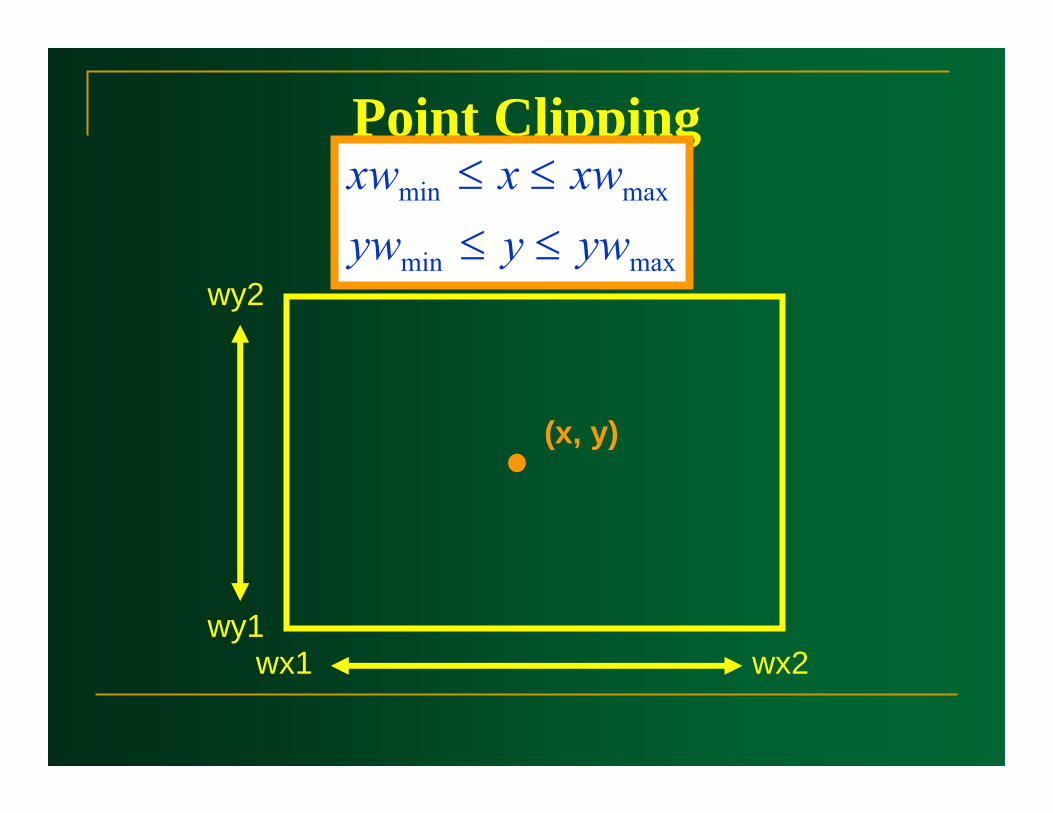
Point Clipping
Point Clipping
(x, y)
wx2wx1wy1
wy2maxmin
maxmin
ywyywxwxxw
≤≤≤≤

Line Clipping
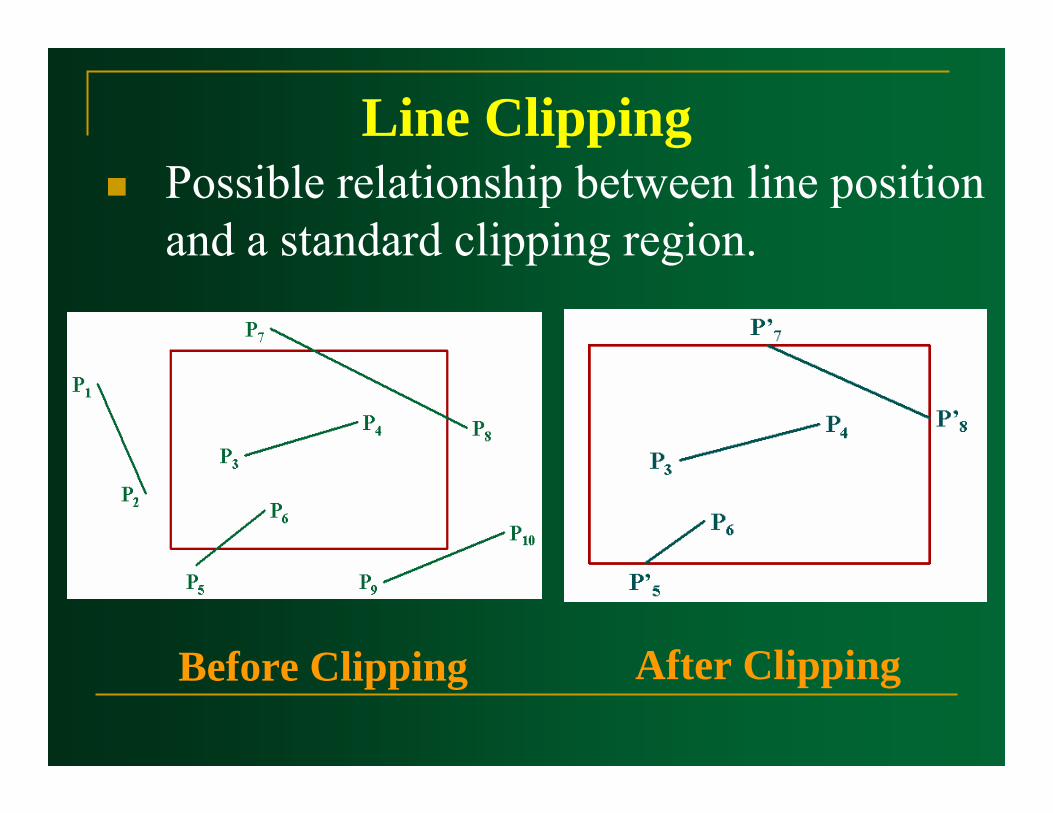
Line ClippingPossible relationship between line position and a standard clipping region.
Before Clipping After Clipping

Line ClippingA line clipping procedure involves several parts:
1. Determine whether line lies completely inside the clipping window.
2. Determine whether line lies completely outside the clipping window.
3. Perform intersection calculation with one or more clipping boundaries.
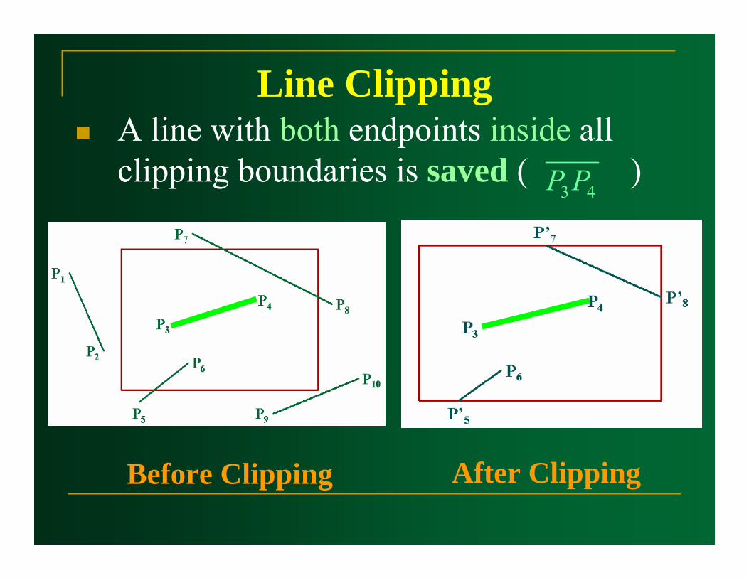
Line ClippingA line with both endpoints inside all clipping boundaries is saved ( )
Before Clipping After Clipping
43PP

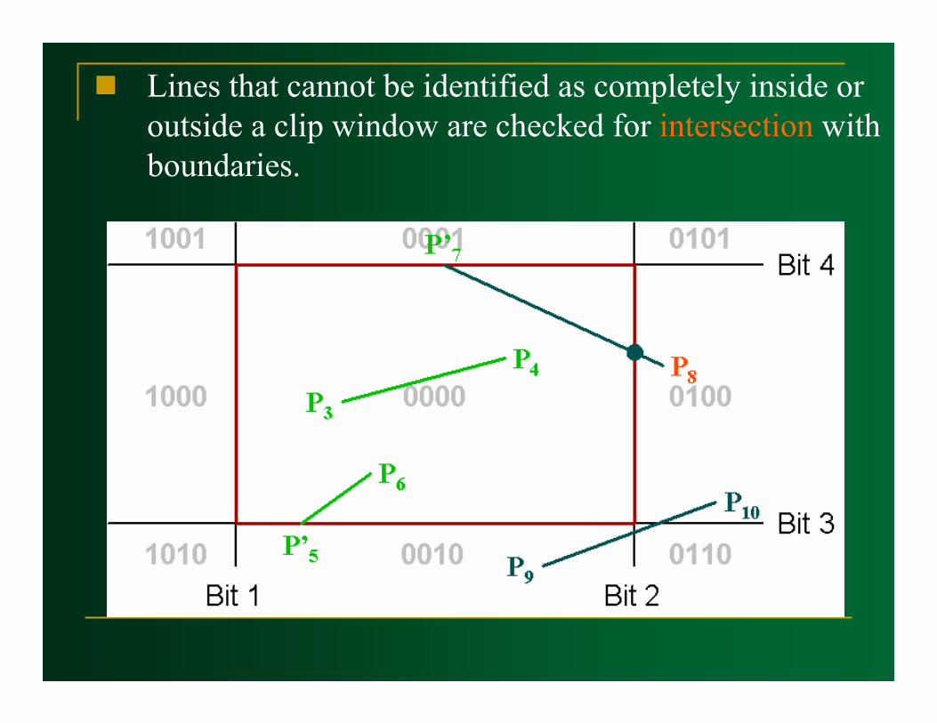
Line ClippingA line with both endpoints outside all clipping boundaries is reject ( & )
Before Clipping After Clipping
21PP 109PP
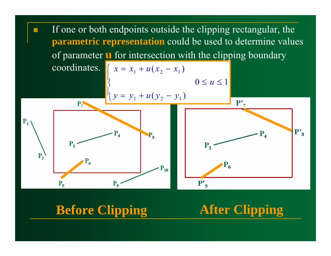
If one or both endpoints outside the clipping rectangular, the parametric representation could be used to determine values of parameter u for intersection with the clipping boundary coordinates.
Before Clipping After Clipping
⎪⎩
⎪⎨
⎧
−+=≤≤
−+=
)(10
)(
121
121
yyuyyu
xxuxx
Line Clipping1. If the value of u is outside the range 0 to 1: The
line dose not enter the interior of the window at that boundary.
2. If the value of u is within the range 0 to 1, the line segment does cross into the clipping area.Clipping line segments with these parametric tests requires a good deal of computation, and faster approaches to clipper are possible.

Cohen Sutherland Line Clipping

Cohen Sutherland Line Clipping
The method speeds up the processing of line segments by performing initial tests that reduce the number of intersections that must be calculated.

Cohen Sutherland Line ClippingEvery line endpoint is assigned a four digit binary code, called region coderegion code, that identifies the location of the point relative to the boundaries of the clipping rectangle.
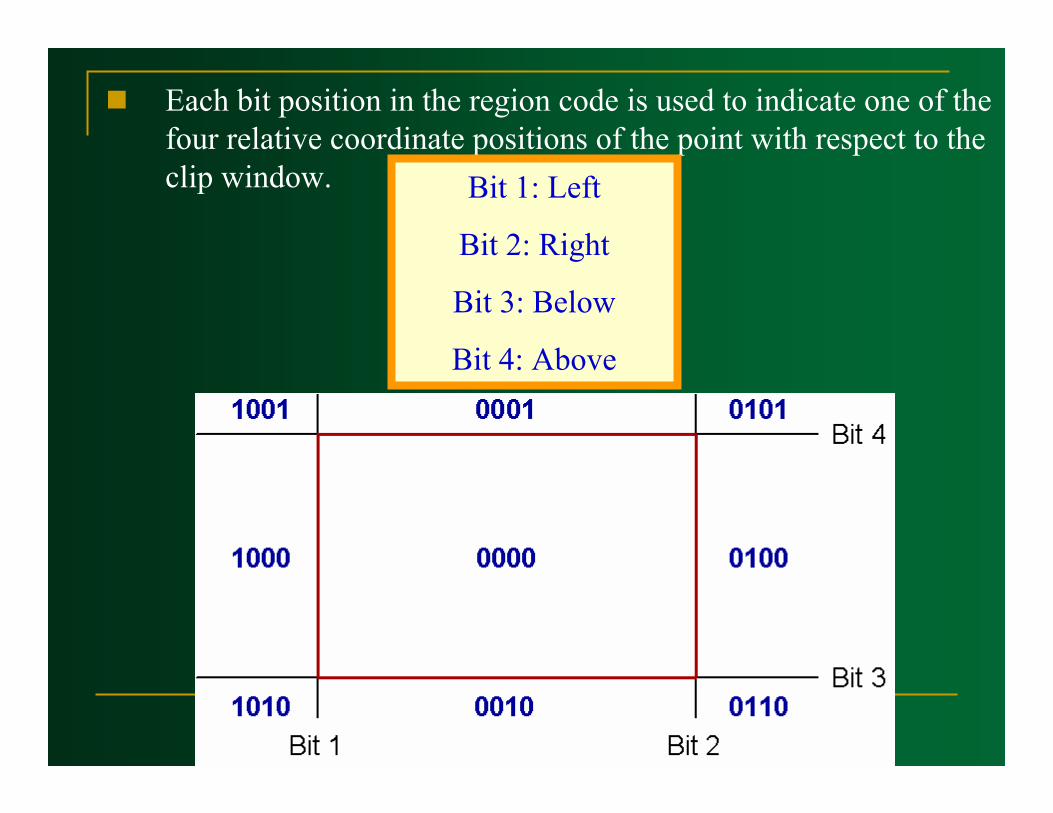
Each bit position in the region code is used to indicate one of the four relative coordinate positions of the point with respect to the clip window. Bit 1: Left
Bit 2: Right
Bit 3: Below
Bit 4: Above
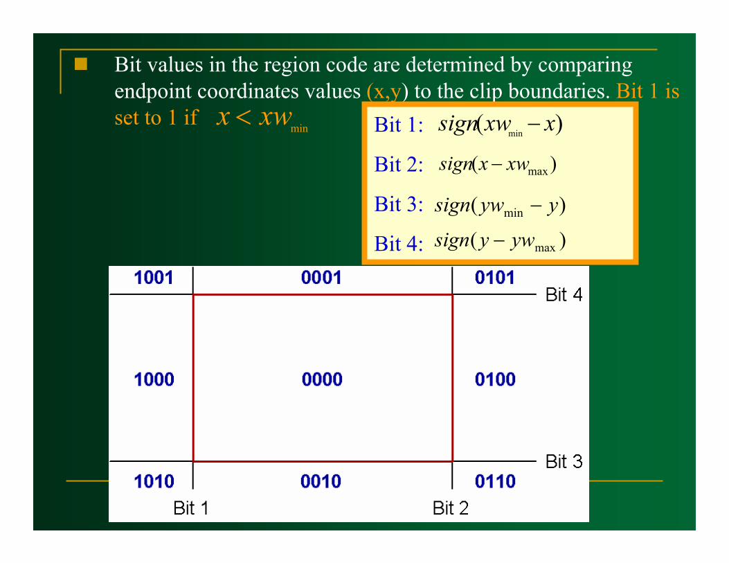
Bit values in the region code are determined by comparing endpoint coordinates values (x,y) to the clip boundaries. Bit 1 is set to 1 if Bit 1:
Bit 2:
Bit 3:
Bit 4:
)( min xxwsign −
)( maxxwxsign −
)( min yywsign −
)( maxywysign −
minxwx <
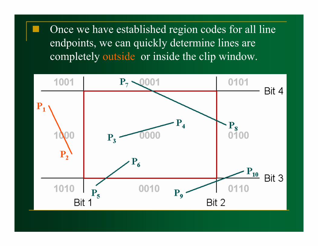
Once we have established region codes for all line endpoints, we can quickly determine lines are completely outside or inside the clip window.

Once we have established region codes for all line endpoints, we can quickly determine lines are completely outside or inside the clip window.

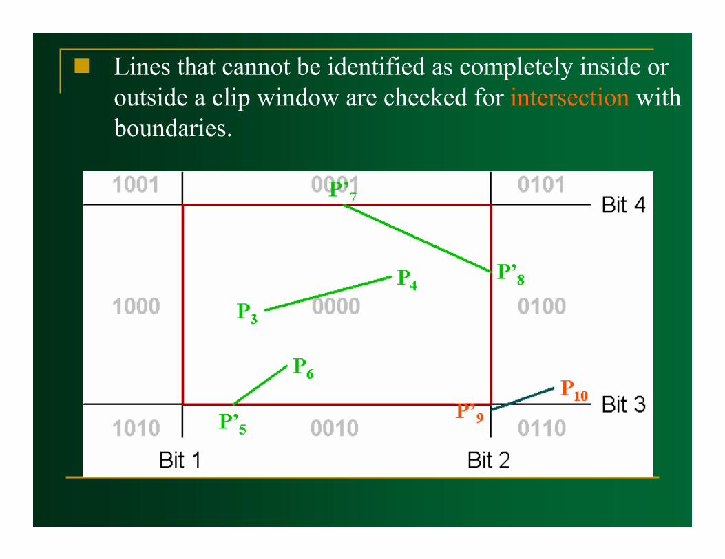
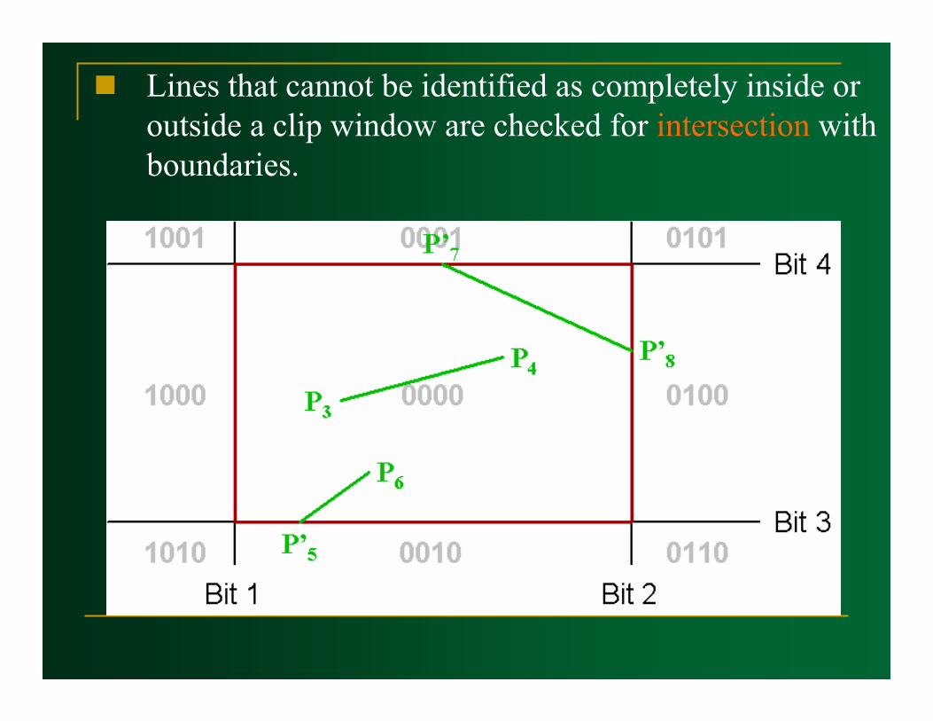
Lines that cannot be identified as completely inside or outside a clip window are checked for intersection with boundaries.
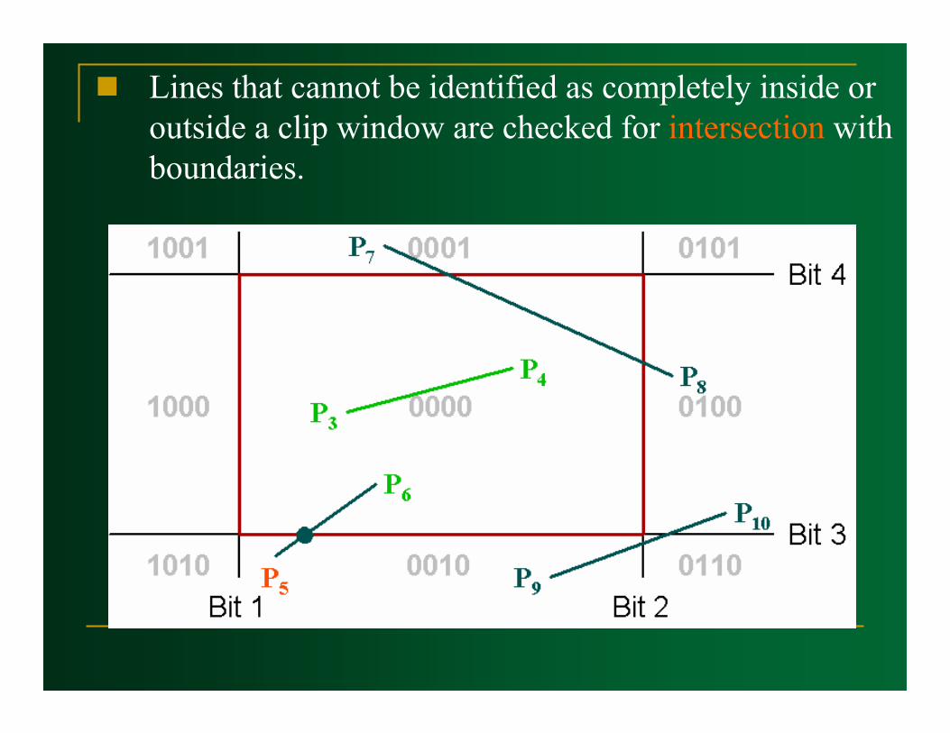
Lines that cannot be identified as completely inside or outside a clip window are checked for intersection with boundaries.

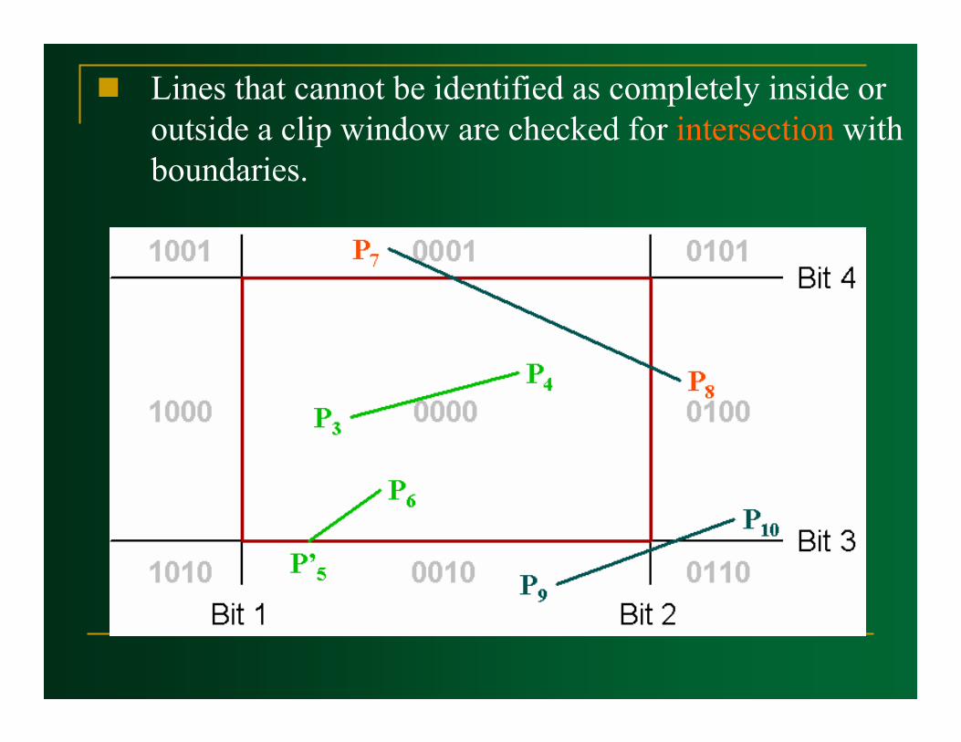
Lines that cannot be identified as completely inside or outside a clip window are checked for intersection with boundaries.

Lines that cannot be identified as completely inside or outside a clip window are checked for intersection with boundaries.
Lines that cannot be identified as completely inside or outside a clip window are checked for intersection with boundaries.

Lines that cannot be identified as completely inside or outside a clip window are checked for intersection with boundaries.

Lines that cannot be identified as completely inside or outside a clip window are checked for intersection with boundaries.
Lines that cannot be identified as completely inside or outside a clip window are checked for intersection with boundaries.

Lines that cannot be identified as completely inside or outside a clip window are checked for intersection with boundaries.

Lines that cannot be identified as completely inside or outside a clip window are checked for intersection with boundaries.

Lines that cannot be identified as completely inside or outside a clip window are checked for intersection with boundaries.

Lines that cannot be identified as completely inside or outside a clip window are checked for intersection with boundaries.
Lines that cannot be identified as completely inside or outside a clip window are checked for intersection with boundaries.

Lines that cannot be identified as completely inside or outside a clip window are checked for intersection with boundaries.
Lines that cannot be identified as completely inside or outside a clip window are checked for intersection with boundaries.
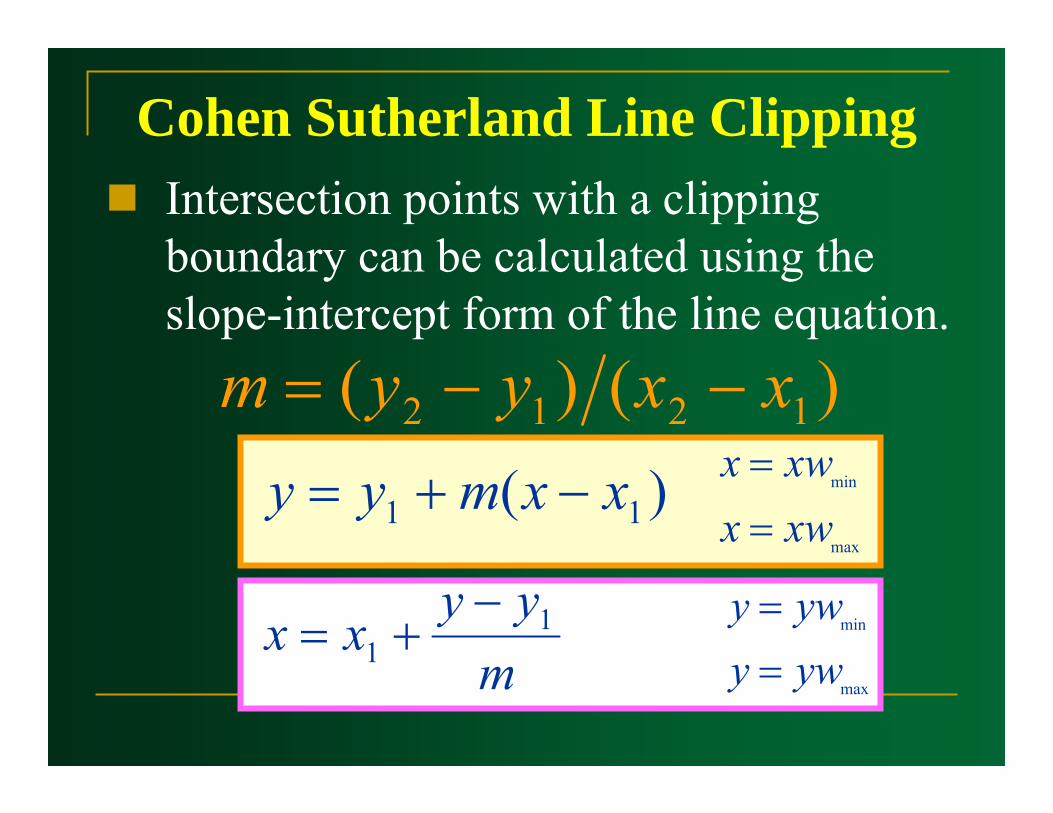
Intersection points with a clipping boundary can be calculated using the slope-intercept form of the line equation.
)()( 1212 xxyym −−=
Cohen Sutherland Line Clipping
)( 11 xxmyy −+=max
min
xwxxwx
==
myyxx 1
1−
+=max
min
ywyywy
==

Liang barskyClipping
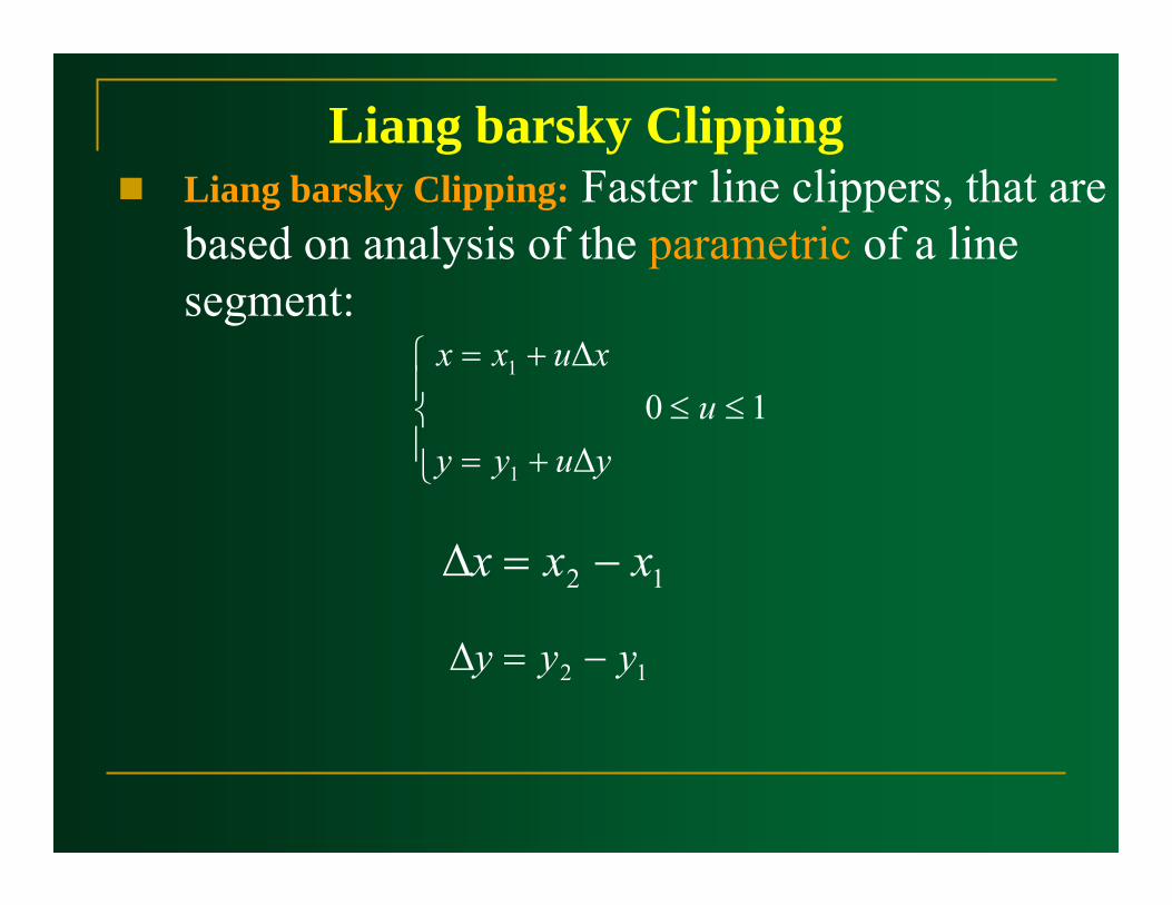
Liang barsky Clipping: Faster line clippers, that are based on analysis of the parametric of a line segment:
Liang barsky Clipping
⎪⎩
⎪⎨
⎧
+=≤≤
+=
yuyyu
xuxx
∆10
∆
1
1
12∆ xxx −=
12∆ yyy −=
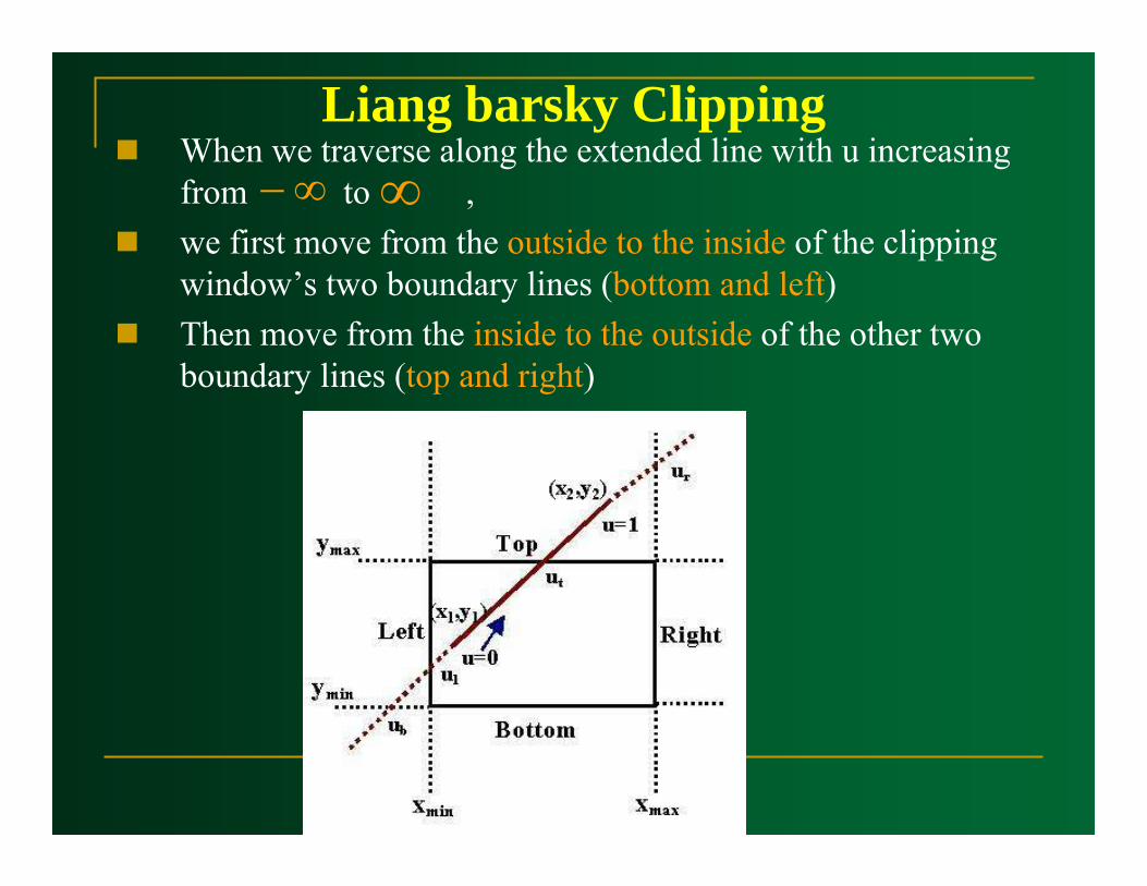
When we traverse along the extended line with u increasing from to , we first move from the outside to the inside of the clipping window’s two boundary lines (bottom and left)Then move from the inside to the outside of the other two boundary lines (top and right)
Liang barsky Clipping∞− ∞
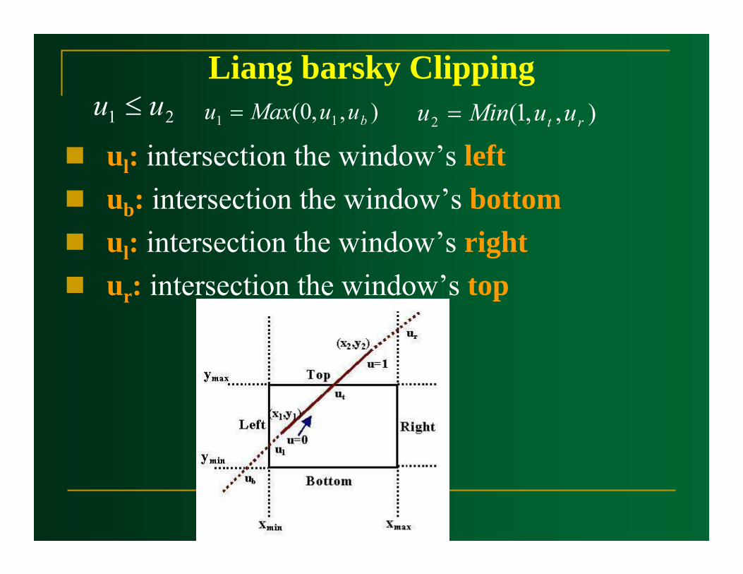
ul: intersection the window’s leftub: intersection the window’s bottomul: intersection the window’s rightur: intersection the window’s top
Liang barsky Clipping21 uu ≤ ),,0( 11 buuMaxu = ),,1(2 rt uuMinu =
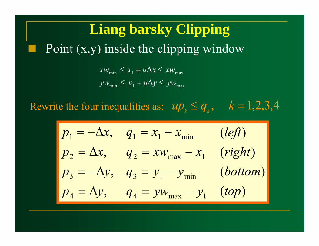
Point (x,y) inside the clipping windowLiang barsky Clipping
max1min
max1min
∆∆
ywyuyywxwxuxxw
≤+≤≤+≤
4,3,2,1, =≤ kqup kk
)()(
)()(
,∆,∆
,∆,∆
1max4
min13
1max2
min11
4
3
2
1
topbottomrightleft
yywqyyq
xxwqxxq
ypyp
xpxp
−=−=
−=−=
=−=
=−=
Rewrite the four inequalities as:
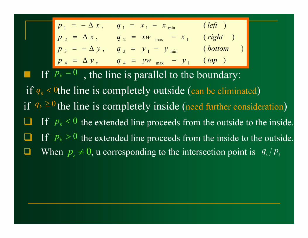
If , the line is parallel to the boundary:if the line is completely outside (can be eliminated)
if the line is completely inside (need further consideration)If the extended line proceeds from the outside to the inside.
If the extended line proceeds from the inside to the outside.When , u corresponding to the intersection point is
)()(
)()(
,∆,∆
,∆,∆
1max4
min13
1max2
min11
4
3
2
1
topbottomrightleft
yywqyyq
xxwqxxq
ypyp
xpxp
−=−=
−=−=
=−=
=−=
0=kp
0<kq0≥kq
0<kp
0>kp
kk pq0≠kp
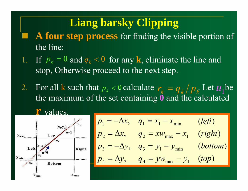
A four step process for finding the visible portion of the line:
1. If and for any k, eliminate the line and stop, Otherwise proceed to the next step.
2. For all k such that , calculate . Let be the maximum of the set containing 0 and the calculated
r r values.
Liang barsky Clipping
)()(
)()(
,∆,∆
,∆,∆
1max4
min13
1max2
min11
4
3
2
1
topbottomrightleft
yywqyyq
xxwqxxq
ypyp
xpxp
−=−=
−=−=
=−=
=−=
0=kp 0<kq
0<kp kkk pqr = 1u
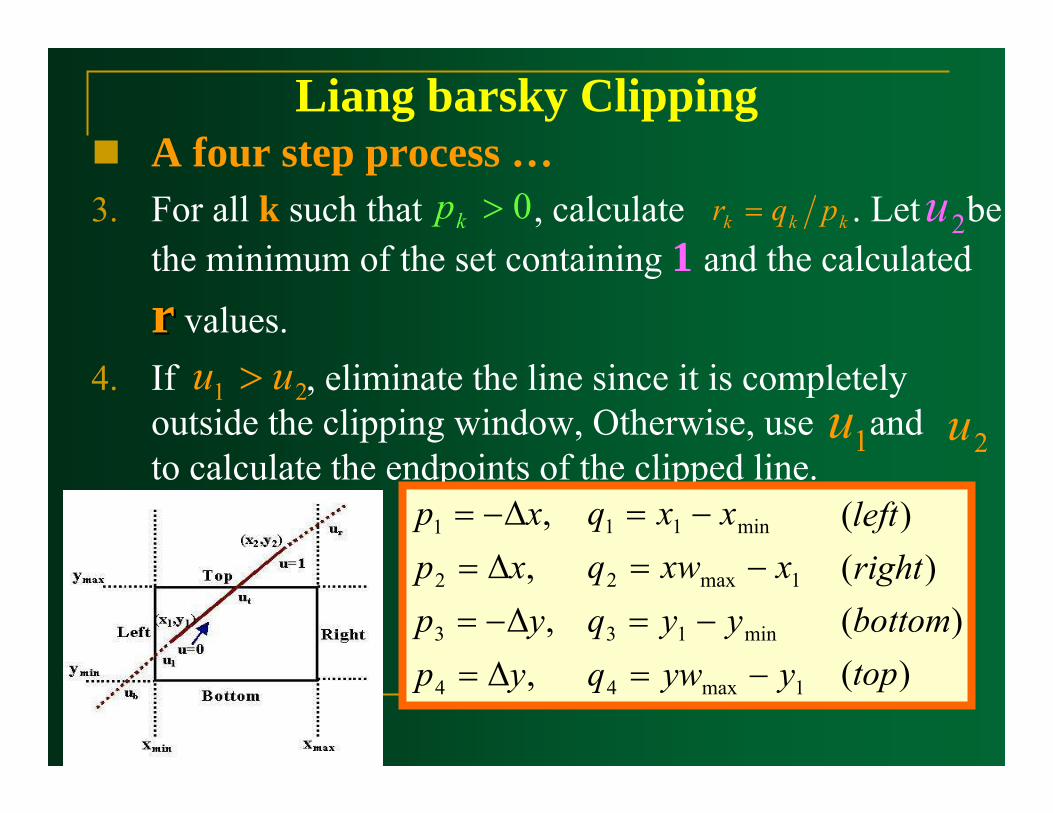
A four step process …3. For all k such that , calculate . Let be
the minimum of the set containing 1 and the calculated
rr values.4. If , eliminate the line since it is completely
outside the clipping window, Otherwise, use and to calculate the endpoints of the clipped line.
Liang barsky Clipping
)()(
)()(
,∆,∆
,∆,∆
1max4
min13
1max2
min11
4
3
2
1
topbottomrightleft
yywqyyq
xxwqxxq
ypyp
xpxp
−=−=
−=−=
=−=
=−=
0>kp kkk pqr = 2u
21 uu >1u 2u


