University of California Santa Barbara
Doctoral Thesis
Tunable Bichromatic Lattices forUltracold Quantum Simulation
Author:
Alan Long
Supervisor:
Dr. David Weld
A thesis submitted in fulfillment of the requirements
for the degree of Bachelors of Science
in the
Weld Lab
Department of Physics
June 2015

Declaration of Authorship
I, Alan Long, declare that this thesis titled, ’Tunable Bichromatic Lattices for Ultracold
Quantum Simulation’ and the work presented in it are my own. I confirm that:
� This work was done wholly or mainly while in candidature for a research degree
at this University.
� Where any part of this thesis has previously been submitted for a degree or any
other qualification at this University or any other institution, this has been clearly
stated.
� Where I have consulted the published work of others, this is always clearly at-
tributed.
� Where I have quoted from the work of others, the source is always given. With
the exception of such quotations, this thesis is entirely my own work.
� I have acknowledged all main sources of help.
� Where the thesis is based on work done by myself jointly with others, I have made
clear exactly what was done by others and what I have contributed myself.
Signed:
Date:
i

“Thanks to my solid academic training, today I can write hundreds of words on virtually
any topic without possessing a shred of information, which is how I got a good job in
journalism.”
Dave Barry

UNIVERSITY OF CALIFORNIA SANTA BARBARA
Abstract
Faculty Name
Department of Physics
Bachelors of Science
Tunable Bichromatic Lattices for Ultracold Quantum Simulation
by Alan Long
We have created and implemented novel methods of quantum simulation. Through uti-
lization of the AC Stark shift, we have developed optical lattices that simulate both
periodic and quasi-periodic ionic lattices. The lattices are highly and precisely control-
lable in situ with minimal size, complexity, and cost.

Acknowledgements
I would like to thank Ruwan Seneratne,Zach Geiger, Kurt Fujiwara, Dr. Boris Shraiman,
Dr. Vyachaslav Lebedev, and my adviser Dr. David Weld for their help and support.
iv
Contents
Declaration of Authorship i
Abstract iii
Acknowledgements iv
Contents v
List of Figures vi
Symbols vii
1 Implementation 1
1.1 Motivation . . . . . . . . . . . . . . . . . . . . . . . . . . . . . . . . . . . 1
1.2 Brief Overview of Lattices . . . . . . . . . . . . . . . . . . . . . . . . . . . 2
1.3 Brief Overview of Experiment . . . . . . . . . . . . . . . . . . . . . . . . . 4
2 Monochromatic Lattices 5
2.1 Physics of optical trapping . . . . . . . . . . . . . . . . . . . . . . . . . . . 5
2.2 Physics of Lattices . . . . . . . . . . . . . . . . . . . . . . . . . . . . . . . 7
3 Bichromatic Lattices 12
3.1 Mathematical Basis of Bicromaticity . . . . . . . . . . . . . . . . . . . . . 13
4 Implementation 19
4.1 Controllability . . . . . . . . . . . . . . . . . . . . . . . . . . . . . . . . . 19
4.2 Apparatus Overview . . . . . . . . . . . . . . . . . . . . . . . . . . . . . . 23
4.3 Measurement of Lattice Parameters . . . . . . . . . . . . . . . . . . . . . 27
4.3.1 Beam Profiling . . . . . . . . . . . . . . . . . . . . . . . . . . . . . 27
4.3.2 Phase measurement . . . . . . . . . . . . . . . . . . . . . . . . . . 28
5 Lattice Characterization 30
6 Conclusion 34
7 Bibliography 35
v

List of Figures
1.1 A classically induced dipole. . . . . . . . . . . . . . . . . . . . . . . . . . . 2
2.1 Atoms are attracted to minima for blue detuned light and maxima forred detuned light. . . . . . . . . . . . . . . . . . . . . . . . . . . . . . . . . 7
2.2 A diagram of two Gaussian beams overlapping at and angle 2φ. Bothbeams propagate from the top of the page to bottom. . . . . . . . . . . . 7
2.3 An example of an optical lattice taken from our camera. . . . . . . . . . . 9
2.4 The same optical lattice. Height corresponds to intensity in arbitraryunits. The x and y axes are in µm. . . . . . . . . . . . . . . . . . . . . . . 10
2.5 A side view of the lattice in Figure 2.3. . . . . . . . . . . . . . . . . . . . . 11
3.1 A bichromatic lattice created with our setup. Lattice C is a superpositionof lattices A and B. Note concurrent maxima and A and B correspond toa maximum in C and similarly with minima. . . . . . . . . . . . . . . . . 12
3.2 An idealization of a bichromatic lattice. The blue is the bichromaticlattice resultant from the red and green lattices. ν = 3
5 . . . . . . . . . . . 13
3.3 The purple is a superposition of the red and blue. . . . . . . . . . . . . . . 14
3.4 The graph of possible energy eigenvalues as opposed to ν, called the Hof-stadter butterfly. . . . . . . . . . . . . . . . . . . . . . . . . . . . . . . . . 18
4.1 A beamsplitter pair, used to create two parallel beams of a controllablespacing. . . . . . . . . . . . . . . . . . . . . . . . . . . . . . . . . . . . . . 19
4.2 An example of a BS pair in our setup. . . . . . . . . . . . . . . . . . . . . 20
4.3 A diagram of the phase modulation apparatus. . . . . . . . . . . . . . . . 22
4.4 The phase modulation in out setup. . . . . . . . . . . . . . . . . . . . . . 22
4.5 A diagram of the main setup. Not to scale. Part numbers refer to thisdiagram. . . . . . . . . . . . . . . . . . . . . . . . . . . . . . . . . . . . . . 23
4.6 A Solidworks model of the setup. This is a slightly different version madefor free space coupling. Beyond the placement of mirrors and lack of fibersit is identical. . . . . . . . . . . . . . . . . . . . . . . . . . . . . . . . . . . 25
4.7 The interferometry apparatus used for phase measurement. . . . . . . . . 28
4.8 The interferometry apparatus as seen from above. . . . . . . . . . . . . . . 29
4.9 The interferometry apparatus at an angle. . . . . . . . . . . . . . . . . . . 29
5.1 Spatial frequency as a function of beam spacing. . . . . . . . . . . . . . . 30
5.2 Lattice slice measured using the razor blade technique. . . . . . . . . . . . 31
5.3 Interferometry measurements and expected values. . . . . . . . . . . . . . 32
5.4 Overnight phase drift. . . . . . . . . . . . . . . . . . . . . . . . . . . . . . 32
vi

Symbols
E electric field N C−1
p dipole C m
U potential J
I intensity W m−2
α dipole proportionality constant unitless
ω angular frequency of light s−1
ω0 angular frequency of optical transition s−1
ν spatial frequency of lattice m
λ wavelength of light m
φ angle of intersection of beams rad
ψ lattice phase rad
Υ envelope function unitless
vii

Chapter 1
Implementation
1.1 Motivation
In the world of condensed matter, crystals are a subject of much importance. Crystals
are seen everywhere and utilized constantly, from piezoelectric drivers to a simple clock.
Crystals are also used as idealizations of solids. The notion of a solid as balls on springs
in a pattern is in many ways the fundamental assumption behind condensed matter.
A crystal can be defined by a pattern, a length scale, and an atom or atoms that form
it. Regrettably all three of these are not easy to control. It is of course impossible
to change the materials making a crystal. The structure is essentially static as it is a
result of the materials in question. Finally, the length scale, e.g. the spacing between
adjacent atoms, can be controlled slightly with thermal expansion and contraction, but
what change may be found is very small and requires large temperature changes.
Because crystals are so useful, we want to discover new crystals with various properties.
However, due to the above reasons, it is difficult to actually create a specified crystal.
It then would seen that some way of crystal simulation would be needed, which must
have certain properties: It must retain the “pattern of balls on springs” behavior, that is
to say the potential must be spatially periodic and approximately a harmonic oscillator
around lattice sites, and it must be able to be controlled, that is to say the pattern,
length scales, and atoms used must all be able to be arbitrarily changed. So before
anything with the actual structure is done, some way of trapping arbitrary atoms must
be found.
1

Chapter 1. Introduction 2
Figure 1.1: A classically induced dipole.
1.2 Brief Overview of Lattices
The immediate answer one might think is to use an electric field. However there are
some problems. First of all, the atoms are neutral, so the best one could hope for is
dipole effects. Secondly, if the field is constant with time, the fact that ∇2V = 0, as we
are working in free space, means that there could not be a minimum or maximum of
the potential except at the boundaries, which is obviously not where we want the atoms
to go. So something must be done to remedy this and actually trap the atoms at a point.
This may be done by utilizing the AC Stark shift. This effect occurs when a dipole is
induced on the atom by an electric field, and then the dipole interacts with that field.
When an atom is in an electric field, the field will pull the electrons in one direction and
the proton in the other as they have opposite charges. This induces a dipole on the atom
proportional to the field. The energy of a dipole p in an electric field E is U = p·E. IF E
is constant, when p will be constant and the atom will simply be in a constant potential.
However, if the field is oscillating, the dipole will as well. In this case U = E · p is no
longer trivially constant, and forms a varying potential. This is the AC Stark shift. So
then, in order to trap an atom, an oscillating field must be used. Luckily there is an
oscillating field that is easy to use and control, light. Light is an electromagnetic wave
and as such will induce an AC Stark shift on the atom. The resultant potential energy
will depend on the intensity of the light, U = AI for a constant A depending on the
atom and light used. This simplifies the trapping problem greatly, instead of needing
to make a periodic potential field, one simply needs to make a periodic intensity. This
may be done through interference.

Chapter 1. Introduction 3
When two beams of light meet they interfere as they are waves. In the simplest case of
two plane waves of the form E = cos(~k · ~x+ ωt) interacting, the resultant intensity is
I = I0 cos2(πx
ν)
Where ν = 2π|k1−k2| is the spatial frequency. As the potential is proportional to the
intensity then
V ∝ cos2(πx
ν)
This is of great use to us. It would appear to satisfy both the periodic requirement
and the harmonic oscillator requirement, as V will be approximately parabolic at the
extrema. Furthermore, it is not reliant on the atom (it turns out the proportionality
constant of the intensity and the potential is, but that only changes the strength not
the function) so it may be used for any atom.
All that is left is the arbitrary pattern, which it does admittedly fail at, and the arbitrary
length scale. The length scale in this equation is ν which, it turns out, is related to the
angle the beams intersect at. So being able to control this angle would give control of
ν, called the spatial frequency.
In addition, though this method cannot make a truly arbitrary pattern, it can do more
than a simple cos2. One might imagine many beams being overlapped forming other
interesting patterns. These beams might all have the same wavelength so they would all
interfere, or pairs of different wavelength so they would not interfere (at a frequency at
atoms could feel), or some combination of the two. Through this many interesting and
physically relevant patterns may be seen. The most simple of which, and the topic of our
research, is two non-interfering patterns overlapping with an irrational periodicity ratio,
i.e. ν1ν2
/∈ Q. This will cause the resultant pattern to be quasiperiodic, structured but
non-repeating. Atoms trapped in such a potential would approximate a quasicrystal, a
quasiperiodic crystal.
So this looks like an appealing method. It satisfied 4.5 of the requirements, it is fairly
straight forward, and it does not require anything unreasonable, simply a good light
source. Because of this, we have used these interference patterns, called optical lattices,
in our research.
These lattices may be used to simulate condensed matter systems. By trapping atoms
in the lattices we can realize many models for ionic lattices, such as the tight binding

Chapter 1. Introduction 4
model and the Hubbard model. Through this we can get a deeper understanding of the
behavior of these systems normally not accessible trough computer simulations.
1.3 Brief Overview of Experiment
It is our goal to simulate such systems. Of particular interest to us are 1 dimensional
quasicrystals realized using quasiperiodic lattices. In order to create this, we use Li
atoms cooled to a Bose Einstein condensate (BEC) in high vacuum. We trap the BEC
in a quasiperiodic lattice with the help of additional traps. We then use the control
ability of the lattice parameters to probe the effects of certain configurations and pa-
rameters. We create this lattice using two pairs of focused laser light, creating two
lattices the superposition of which is quasiperiodic. We believe this set up will realize a
quasiperiodicity in atoms in a controllable manner and greatly further our knowledge of
quasicrystals.

Chapter 2
Monochromatic Lattices
2.1 Physics of optical trapping
In order to work with atoms, there needs to be a way of controlling them. One can
obviously not bolt an atom to a breadboard. What we need is some sort of potential,
and subsequently some sort of force, to keep the atoms where we want them. It seems
like the obvious solution would be to use some field force, which does end up being the
right answer, but with some difficulties. There is only one such force we are able to
manipulate with any ease, the electromagnetic force, so that is an obvious choice of tool
when compared to say, gravity. However we face the immediate issue of the fact we are
using neutral atoms. This means we can, at best, get dipole effects. So, looking back
on what we need. We need to induce dipoles on atoms, we need to use those dipoles to
put the atoms in a potential, and that potential needs to be controllable and confine the
atoms to a region. How might one do this, you may ask. Well it’s in the next section.
Let there be an oscillating electric field. Using complex notation,
~E = EEeiωt
Where E is the direction of polarization and E is the complex magnitude. Any dipole
induced by this field must be proportional to the field. So
~p = α~E
p = αE
for some complex α, called the polarizability. For any induced dipole the potential is
U = −1
2〈pE〉
5

Chapter 2. Monochromatic Lattices 6
U = −1
2〈α(Eeiωt)2〉
U = −1
2Re(α)|E|2
So then we get non trivial potential, which is what we wanted. So, an oscillating electric
field is the answer to our problem. It should be apparent that light fits the bill. In this
case the potential becomes
U =1
2ǫ0cRe(α)I
where I is the intensity of the light. However we still do not know what α is. By looking
at power absorption and scattering rates, it turns out that α can be found, and that it
depends on the atom being trapped and the the transitions in the atom. We can simplify
this by utilizing Lorentz’s classical oscillator model. Specifically, the constant is
α = 6πǫ0c3 Γ
ω40 − ω2ω2
0 − iω3Γ
Where ω is the frequency of the light, ω0 is the frequency associated with the opti-
cal transition and also the eigenfrequency of the classical oscillator model, and Γ is a
damping constant due to dipole radiation. It is
Γ =e2ω2
0
6πǫ0mec3
If we assume that Γ is small, i.e. the dipole radiation is negligible, the expression may
be reduced. This is a valid approximation as the coefficient in front of the ω20 in the
expression is approximately 6× 10⁻²⁴s. So making this approximation, α becomes real,
and may be simply plugged into the expression for U to get
U =3πc2Γ
ω20(ω
2 − ω20)I
U =e2
2cǫ0me(ω2 − ω20)I
Note the sign of the expression. All constants and I are positive, so the sign is deter-
mined by the difference in squares of the frequencies. If ω > ω0 the potential will be
greater the greater the intensity, meaning atoms are repelled from areas of high inten-
sity. Conversely, ω < ω0 means that a high intensity corresponds to a low potential, and
atoms are attracted to high intensity. These are referred to as blue detuned and red
detuned respectfully. The effect that they would have on atoms can be seen in Figure
2.1

Chapter 2. Monochromatic Lattices 7
Figure 2.1: Atoms are attracted to minima for blue detuned light and maxima forred detuned light.
For the blue detuned case the atoms tend to the intensity minima and in the red detuned
case they tend to the maxima.
2.2 Physics of Lattices
Let’s leave the math of trapping for a bit and look at interference. It turns out that
interference patterns end up being quite useful, as we’ll see in a moment. Suppose that
there are two Gaussian beams overlapping at their waists as in Figure 2.2.
We’ll make some assumptions and definitions about the beams. First, assume the
Figure 2.2: A diagram of two Gaussian beams overlapping at and angle 2φ. Bothbeams propagate from the top of the page to bottom.

Chapter 2. Monochromatic Lattices 8
beams propagate from the top of the page to the bottom. Let the beams intersect at an
angle 2φ as shown. Let the beams have the same intensity, and the same wavelength λ.
Let the beams differ in phase by 2ψ. Assume that the beams are both linearly polarized
into the page. Finally assume that the beams are Gaussian and that they are uniform in
the region where they overlap, that is we need not consider the beams spreading. This
seems like a lot, but the only real approximation we made was that the beams were
uniform at their waists, which is true up to first order. The rest is just definitions or
things that can be controlled in an experiment.
Moving forward, these beams will interfere and form a standing wave. By symmetry the
pattern must be constant, bar the envelope function, in the y or z directions. So then
we can consider the x direction alone. Both beams will be of the form
E = E0er2
ω20±(ikl+ψ
2)+iωt
Where w0 is the waist, k is the wave vector, and r, l are cylindrical coordinates. If we
only concern ourselves with the plane perpendicular to their combined wave vectors, i.e.
the x− z plane, the equation becomes
E = E0e−x2cos(φ)2+z2
ω20±i(kxsin(φ)−ψ)+iωt
Adding the two gives
E = E0e−x2cos(φ)2+z2
ω20+iωt (
eikxsin(φ)−ψ + e−ikxsin(φ)+ψ)
E = 2E0ex2cos(φ)2+z2
ω20+iωt
cos
(
2π sin(φ)
λx− ψ
)
Squaring the norm to get intensity gives
I = 4E20e
2x2cos(φ)2+z2
ω20 cos2(
2π sin(φ)
λx− ψ
)
I = 4E20e
2x2cos(φ)2+z2
ω20 cos2(
2π sin(φ)
λx− ψ
)
So, from equation relating intensity and potential above
U =12πc2Γ
ω20(ω
2 − ω20)E2
0e2x2cos(φ)2+z2
ω20 cos2(
2π sin(φ)
λx− ψ
)

Chapter 2. Monochromatic Lattices 9
For ease’s sake lets define
U0 =12πc2Γ
ω20(ω
2 − ω20)E2
0
Υ = e2x2cos(φ)2+z2
ω20
ν =λ
2 sin(φ)
Then the equation is
U = U0Υcos2(πx
ν− ψ)
Which is much cleaner. We see that the equation has three main parts. First a scaling
constant U0 related to the set up and atom, then an envelope function Υ, and finally a
periodic pattern, the cos2 term, with frequency ν and phase −ψ. Figure 2.3 is a picture
Figure 2.3: An example of an optical lattice taken from our camera.
of an actual lattice created in lab. Figure 2.4 a visualization of data gathered using our
set up, with height corresponding to potential (with arbitrary units) and the x and y
units in µm. Note the Gaussian envelope and the periodic nature. We call this pattern
an optical lattice.
Figure 2.5 shows a side view of the lattice above, with U0 and ν labeled. For a single
1-dimensional lattice such as this, these are the most important parameters. In our
experiment we try to make the lattice as wide as possible so there will be a large section
where Υ ≈ 1, as then the lattice is completely periodic. In this case, the phase of the
lattice does not matter as it is symmetric under translation. This leaves well depth and
spatial frequency as the two most important values that define a lattice.

Chapter 2. Monochromatic Lattices 10
Figure 2.4: The same optical lattice. Height corresponds to intensity in arbitraryunits. The x and y axes are in µm.
So, at least in one dimension and assuming Υ ≈ 1, we have atoms being affected by a
periodic potential. This should bring to mind crystals. Crystals are, at their simplest,
periodic patterns of atoms. Atoms trapped in the lattice would tend to the maxima of
the lattice, assuming red detuning. We will assume that the lattices are red detuned
unless otherwise noted. Blue detuning would lead to identical situations, but with atoms
at minima. This would create a pattern of equally spaced atoms, essentially equivalent
to a crystal with lattice constant ν. The analogy becomes even better. To second order,
cos2(kx) = 1 − k2x2 at a maximum. Which means that the potential will be approx-
imately quadratic at the lattice sites, as one might expect. This is impotent however,
because it means that the quantum system is approximately a harmonic oscillator. It is
very common in condensed matter to model atoms in an ionic lattice as in a harmonic
oscillator at each lattice site. When in an optical lattice, atoms will experience the same
effects, modeling the behavior of an ionic lattice. This correspondence is the reason for
the name ”optical lattice” and why terminology of the two may be interchanged. Optical
lattices then simulate the behavior of crystals both on a large scale, where the lattice
structure is most important, and a small scale, where the behavior of atoms at a given
lattice site is most important.

Chapter 2. Monochromatic Lattices 11
Figure 2.5: A side view of the lattice in Figure 2.3.
This is incredibly useful. It is very rare that a complicated system can be completely
solved. Most often, it must be solved numerically. In many cases, specifically cases with
strongly interacting particles, the computations needed to model the system evolving
with time become prohibitively large. Because of this, computer simulations are capped
at a certain point. If one were to have a lattice with a Hamiltonian similar to that of
an ionic lattice, it would evolve in time similarly to the actual crystal. Through this it
is possible to model the effects on an ionic lattice over a much greater time span than
with computers.
This method may be used for many models. If the well is sufficiently deep, tunneling will
be small. This means that interactions between lattice sites will also be small. Because
of this electrons will stay close to a particular lattice site and thus with a particular atom.
This is a realization of the tight binding model. It can be shown that the Hubbard model
can also be realized using lattice.

Chapter 3
Bichromatic Lattices
Figure 3.1: A bichromatic lattice created with our setup. Lattice C is a superpositionof lattices A and B. Note concurrent maxima and A and B correspond to a maximum
in C and similarly with minima.
A very interesting and useful implementation of lattices is creating superpositions of
them, forming superlattices. This can create many interesting patterns and effects.
This simplest case of this is a bichromatic lattice, the superposition of two lattice with
the same direction but different spatial frequencies. It is called a bichomatic lattice due
to the fact that is could be formed with two different colored beam pairs interfering, but
it is easier to create it with same color beams. This can be done by having the pairs
intersect at the same spot but at different angles, which is the method we have used in
our experiments.
12
Chapter 3. Bichromatic Lattices 13
However,how exactly could this be done? If you had four beams crossing each would
interfere with every other one, making 6 lattices, not just the two wanted. This can
be solved in two ways. First, the polarizations between pairs may be made orthogonal.
This would mean that a beam would only meaningfully interfere with the other beam of
its pair, The other method would to have the wavelengths of the beams slightly detunes
from one another. Though the beams would interfere, the interference would oscillate
so rapidly that the atoms would not be affected by it.
3.1 Mathematical Basis of Bicromaticity
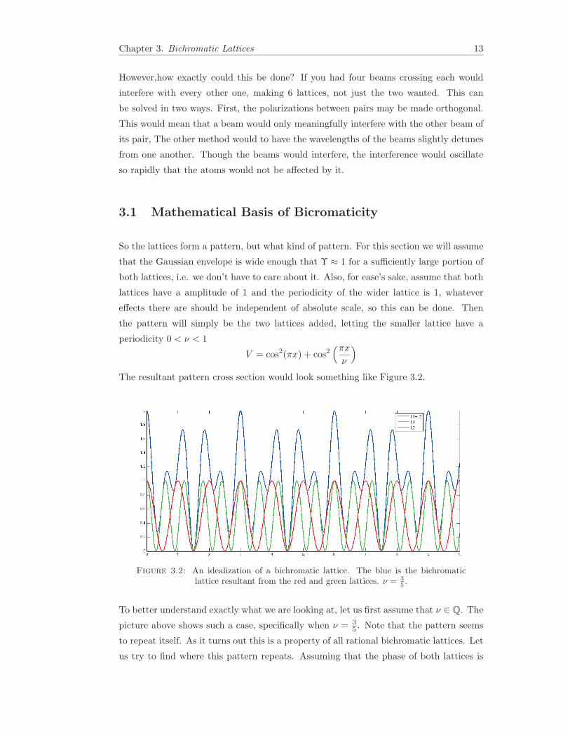
So the lattices form a pattern, but what kind of pattern. For this section we will assume
that the Gaussian envelope is wide enough that Υ ≈ 1 for a sufficiently large portion of
both lattices, i.e. we don’t have to care about it. Also, for ease’s sake, assume that both
lattices have a amplitude of 1 and the periodicity of the wider lattice is 1, whatever
effects there are should be independent of absolute scale, so this can be done. Then
the pattern will simply be the two lattices added, letting the smaller lattice have a
periodicity 0 < ν < 1
V = cos2(πx) + cos2(πx
ν
)
The resultant pattern cross section would look something like Figure 3.2.
Figure 3.2: An idealization of a bichromatic lattice. The blue is the bichromaticlattice resultant from the red and green lattices. ν = 3
5.
To better understand exactly what we are looking at, let us first assume that ν ∈ Q. The
picture above shows such a case, specifically when ν = 35 . Note that the pattern seems
to repeat itself. As it turns out this is a property of all rational bichromatic lattices. Let
us try to find where this pattern repeats. Assuming that the phase of both lattices is

Chapter 3. Bichromatic Lattices 14
0, they will both have a maximum when x = 0 so then we simply need to find the next
dual maximum. cos2 has its maxima when its argument is nπ where n is any integer.
So wider lattice will have a maximum every integer. So it is simply finding an integer
n s.t. νn ∈ N. As ν ∈ Q, ν = pqfor some p, q ∈ N where p and q are mutually prime.
So then if nqp
∈ N then p|nq but as q is mutually prime to p, p|n. So then the smallest
integer s.t. the pattern returns to its maximum is p. We can observe this in Figure 3.2.
I said earlier that the picture was of the case where ν = 35 and in fact, as you can see,
there is a maximum where x = 3 and this is the first maximum. So then the case where
ν is rational is fairly straightforward.
However, the irrational case is, luckily, far more interesting. Though the above work
will obviously not work directly for this case, it can be used for approximations. An
irrational number may be approximated using rational numbers, by continued fractions
or decimal expansion or any other such way. So then, as we consider shorter lattices
with spatial frequencies increasingly close to the irrational value we want, the resultant
bichromatic lattice should get closer and closer to the one we want. However, as the ra-
tional approximation nears the irrational number, the numerators get increasingly large,
meaning that the limit of the repetition distance as the periodicity ratio becomes irra-
Figure 3.3: The purple is a superposition of the red and blue.
tional goes to infinity. So then two lattices with irrational spatial frequencies will never
have their pattern repeat. This means that the pattern is no longer periodic, and is
now quasiperiodic. That is to say it is ordered, but not strictly periodic. This is very
interesting because the atoms loading into the trap will form into this pattern. So, like
the atoms in the, periodic, monochromatic lattice formed a crystal, these atoms would
form a quasicrystal. Quasicrystals are the subject of much research and are still being
found. Having the ability to simulate not just quasicrystals but custom order quasicrys-
tals would be a massive boon for our knowledge on a subject. Luckily this is what
these quasiperiodic lattices offer. Of particular interest to us are lattice where the ratio

Chapter 3. Bichromatic Lattices 15
between the lattices is the golden ratio, φ = 1+√5
2 , as we will show shortly.
We now know quasiperiodicity is created by irrational ν and any irrational ν will make
a quasi periodic lattice. One might now ask, does the choice of ν matter? It would be
very convenient if ν could be set to any irrational number and have the same effects.
This is regrettably not the case. Consider ν = 12 +
√2
10000 . This is irrational and will
make quasiperiodic lattice, however it will be very close to the lattice created by ν = 12 .
Quantitatively, the peaks will be .05 away, a good estimate for ”significant”, from each
other at x ≈ 35.5. Meaning that within any given 35 long interval, the quasiperiodic
lattice looks the same as the rational lattice, but with some phase. This means that
any quasiperiodic effects will not be evident on any scales of that size or smaller. These
effects are the reason we want these superlattices so a lattice like this would not allow
for any experimentation to be done. This is an example of a ratio we do not want, a
“bad choice” of ν.
So then, how do we get good choices. Let’s take a step back and think about an irra-
tional lattice mathematically. As rational lattices are much easier to work with, it would
be beneficial to find rational approximations. Though there are many ways to go about
this, it turns out that the method of continued fractions is both the easiest and the most
helpful.
Any real number x may be expressed as a continued fraction of the form
x = a0 +1
a1 +1
a2+1
...+ 1an
if x is rational and
x = a0 +1
a1 +1
a2+1
...
if x is irrational, with a0 ∈ Z and ai ∈ N when i > 0. By truncating at some an, one
can create a rational approximation of an irrational number x. That is to say, is x is
defined as above in the irrational case, the approximation, call it xn would look like the
rational case above.
So then, if ν is some irrational ratio of spatial frequencies, it may be expressed as a
continued fraction. As ν is defined to be 0 < ν < 1, disregarding the case where ν = 1
as it is trivial, we know that a0 = 0 for any ratio. Let us similarly define νn as the
continued fraction truncated at the nth entry. νn ∈ Q so νn = pqfor some p, q ∈ N. To

Chapter 3. Bichromatic Lattices 16
find what these are, we can use induction. Consider just looking at the partition of ai
where i > j for some j. This part will be
aj +1
· · ·+ 1an
This will obviously be rational, let it befnjgnj
, where the superscripts denote the fact we
are considering νn, not showing powers. Note that the fractional part of the expression
will be1
aj+1 +1
···+ 1an
=gnj+1
fnj+1
So we have
aj +gnj+1
fnj+1
=fnjgnj
So
fnj = ajfnj+1 + gnj+1
gnj = fnj+1
Looking at j = n we see fnn = an and gnn = 1. This process can be done to find fn1 and
gn1 . Putting these into the original equation gives
νn =1fn1gn1
=fn2fn1
So then a lattice of this ratio would have a repetition distance of fn2 (if n = 1 we define
f12 = 1).
Now we have a method of approximating irrational lattices and characterizing those
approximations, and so we can start to answer the very aforementioned question “what
is a ‘good” lattice?”. What went wrong with the bad example above was that distance
between repetition for some successive approximations was very large, making there be
a large gap in necessary length scale for the lattice to noticeably change. So what we
want is for any given successive difference to be as small as possible. This can be done
using strong induction. First the base case, n = 2. So we are trying to minimize f22 −f12 ,
however this is just a2 − 1, and the minimal natural number is 1 so a2 = 1. Now for
induction, assume ai = 1 for 1 < i ≤ n. We are again trying to approximate fn+12 − fn2 .
However as fn2 is set by our inductive hypothesis, this is the same as minimizing fn+12 .
As ai = 1 when 1 < j < n+ 1,
fn+1j = fn+1
j+1 + fn+1j+2
Chapter 3. Bichromatic Lattices 17
. With fn+1n+1 = an and fn+1
n+2 = 1. This has a closed form solution of
fn+1n−m = F (m+ 1)an+1 + F (m)
where F (m) is themth Fibonacci number. This is have a minimum again when an+1 = 1
so that must be the case. So by induction ai = 1 when i > 1. The case where ai = 1
for every i ≥ 0 is the continued fraction of φ, the golden ratio. So ν = 1a1+φ−1 . When
a1 = 1 this is just ν = φ−1.
So now we have a target periodicity ratio so that the successive distances of repetition
are minimized. Not unsurprisingly it minimizes the ais. In fact, it is generally true that
numbers with one or more large ais will be “bad”. For example, 12 +
√2
10000 from above
has a1 = a2 = 1 but a3 = 1767. So then there is a massive jump from the second ap-
proximation resolution distance to the third. which is the jump from ν ≈ 12 to a better
approximation, which is what we saw earlier.
This is one reason why the golden ratio is so interesting and why the work above actually
matters. The golden ratio will have its large n approximations be used the earliest,
making its quasiperiodic behavior “appear” on the shortest scale. Because we have
limited scale, this means such a lattice will be the most quasiperiodic possible. This
lattice is so interesting it has its own name, a Fibonacci lattice. It is so called because
approximations of the golden ratio are the ratio of successive Fibonacci numbers, which
can actually be seen above
fn+1j = fn+1
j+1 + fn+1j+2
This is simply the definition of the Fibonacci sequence, as its starts with 1,1 as proved.
As said before, quasiperiodic lattices can be used to realize quasicrystals. There is
much research currently being done on quasicrystals. There are hundreds of known
quasicrystals, which in the grand scheme of things is actually quite small. Quasicrystals
were only discovered in 1982, a discovery which would later win the 2011 Nobel prize.
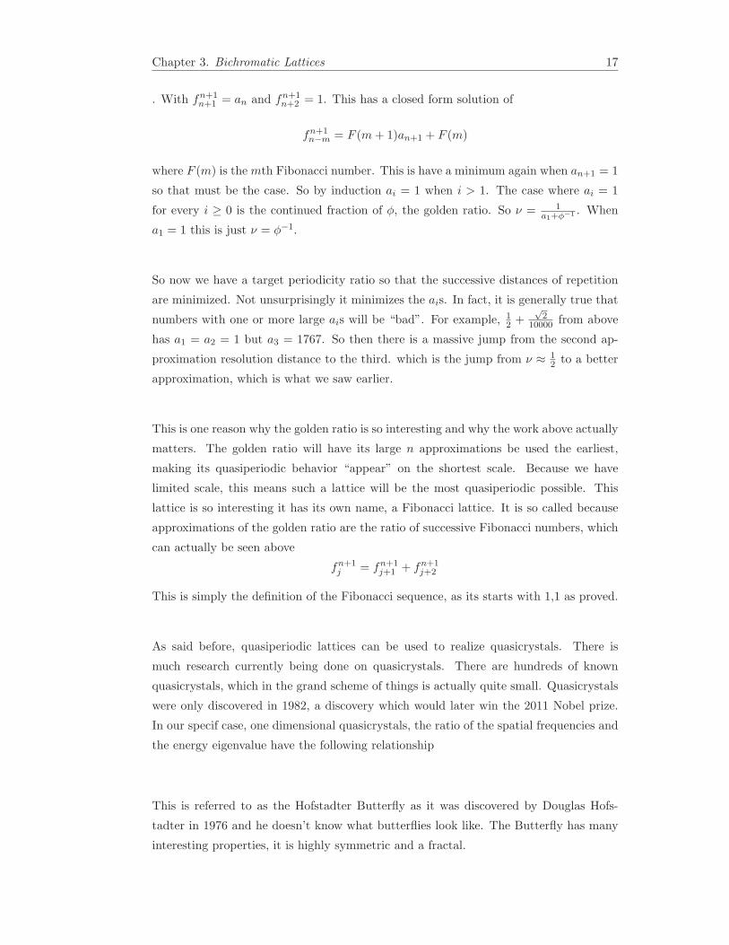
In our specif case, one dimensional quasicrystals, the ratio of the spatial frequencies and
the energy eigenvalue have the following relationship
This is referred to as the Hofstadter Butterfly as it was discovered by Douglas Hofs-
tadter in 1976 and he doesn’t know what butterflies look like. The Butterfly has many
interesting properties, it is highly symmetric and a fractal.
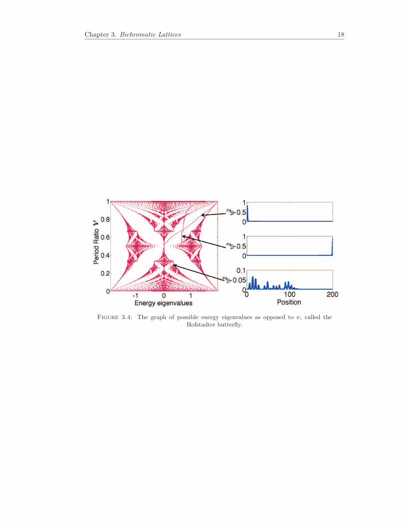
Chapter 3. Bichromatic Lattices 18
Figure 3.4: The graph of possible energy eigenvalues as opposed to ν, called theHofstadter butterfly.

Chapter 4
Implementation
4.1 Controllability
Figure 4.1: A beamsplitter pair, used to create two parallel beams of a controllablespacing.
In order to create the lattice, we utilize a method originally created by Foote, a beam
splitter pair. Figure 4.1 shows a diagram of the prototypical pair. Looking first at
the red beam, the beam is sent into the pair from the right. It first passes through
a λ/2 waveplate. The waveplate is rotated such that an equal amount of power will
be retroreflected and transmitted by the right beamsplitter. The beam then hits the
cube, half is reflected out to a lens, which we will return to, and half is transmitted.
As the transmitted beam is polarized such that it passes through the first beamsplitter,
19

Chapter 4. Implementation 20
Figure 4.2: An example of a BS pair in our setup.
it will pass through the second entirely. the beam then passes through a λ/4 wave-
plate, is reflected off a mirror, and passes though the waveplate again. The waveplate
is rotated such that it causes the polarization of the beam to be rotated 90◦. As it
is now orthogonal to how it was originally, and that was entirely transmitted, it will
now be entirely reflected by the left beamsplitter. It then joins the other reflected beam
on the lens. The lens focuses the beams to a point, where they interfere creating a lattice.
This set-up has many advantages. First, the beams are inherently parallel. Because the
beamsplitters will form essentially two mirrors orthogonal to one another, the beams will
be parallel, even if the beam does not come in perfectly normal to the cube face. This
both makes set up easier, as it takes away a degree of freedom that would otherwise
need to be exact, and it allows for the outgoing beams to be directed to the left or
right slightly. In addition, the set up is compact. In our final apparatus, we had two of
these pairs, along with all other necessary optics, fitted to a 10 by 12 inch breadboard.
Furthermore, it makes power control easy. Because the two outgoing beams are a set
fraction of the incoming beam, the outgoing beams will always have the same relative
power, and to change their power is simply a matter of changing the incoming beam.
This is immensely useful as beams of different powers will not create a good lattice, as the
wells will no be as deep as they could be due to the part of the stronger beam not canceled
by the weaker. This both allows for better lattices, and makes power modulation, for

Chapter 4. Implementation 21
example a noise eater, easy to adapt to the set up. Finally, the set up makes predicting
the periodicity very easy. In order to know the periodicity, you of course need to know
at what angle the beams interfere. This is somewhat difficult to measure in practice.
However, with this set up, one simply needs to know the spacing between beams, which
is easily measured, and the focal length of the lens, which is known, to figure out the
angle using simple trigonometry. If the beam comes in x distance from the cube faces
the periodicity is
ν =λ
2 sin(
tan−1(
xf
))
where f is the focal length. This is, at least in comparison to the other expressions we’ve
used, very simple. Through this it is easy to get a quick approximation of the periodicity.
Of course, this is not a very exact method, and much better ways of measuring periodicity
will be talked about at length, but this is a very good check to make sure you’re at least
in the ballpark of your intended value.
In addition to these, this set-up makes the lattice very easy to tune. To see this consider
the green beam. In practice the two beams being shown in would be the same color,
but they are different here for visualization purposes. If the red beam is some distance
x above the from of the pair, the green beam is x + ∆x away. The green beam goes
through the apparatus exactly as the red beam, and similarly comes out in two halves
into the lens. However, It will be the same distance from the center line as it was from
the cube faces, x+∆x. Because of this, it will be at some angle φ+∆φ. As the angle
has changed, the lattice will have a different periodicity, with the new value being
ν +∆ν =λ
2 sin(
tan−1(
x+∆xf
))
So by simply changing the position of the beam (or by changing the position of the
cubes), the periodicity may be easily controlled. This is very helpful because beam/cube
position can be controlled using movable stages, which are readily accessible, accurate,
and programmable. This is a simple, elegant solution to the problem of period control.
Of course, period is not the only thing of interest. As stated above there is also trap
depth and phase. Trap depth is very easy to control, just increase the power of the
beams, but phase modulation requires more work. Phase modulation of the lattice is
achieved through phase modulation of one of the beams, in this case the retroreflected
one. The movement of the mirror will change the path length, thus changing the phase.
Specifically, is the mirror is moved some distance ∆x, the path length will change by
2∆x, because the incident beam and the reflected beam are both changed by ∆x. This
will result in a phase change of the beam by ψ = 2∆xλ
.
This will result in a change in phase of the lattice. This is due to the fact that the

Chapter 4. Implementation 22
Figure 4.3: A diagram of the phase modulation apparatus.
Figure 4.4: The phase modulation in out setup.
locations of the maxima of the beam has now changed, so the places where both beams
are at their maxima, i.e. the maxima of the lattice, will also spatially change. If you
were looking at the lattice as the mirror was slowly moved, you would see the maxima
appear to translate across the screen, but have the Gaussian envelope stay in its place.

Chapter 4. Implementation 23
Figure 4.5: A diagram of the main setup. Not to scale. Part numbers refer to thisdiagram.
4.2 Apparatus Overview
The beam is emitted by the laser. It is then sent through a fiber optic cable two two
parallel and identical setups. The light it then recollimated with two fiber collimators
(1,3). It then is reflected off of mirrors (2,3) and then passes through beam samplers
(6,8) splitting off a small fraction of the beam onto photodiodes (5,7). The signal from
the photodiode is then sent to a noise eater which modulates the power of the corre-
sponding beam, correcting for any power fluctuations. There is a parallel identical set
up that creates another beam. This beam is also modulated in a similar way using a
noise eater
Both beams will pass through beamsplitter pairs (9-18), creating two beam pairs. For
both of these beamsplitter pairs, the retroreflective mirrors (14,17) is attached to a
piezoelectric crystal (15,18). This allows for the optical path length of the retroreflected
beam coming from the beamsplitter pair to have its optical path length changed thus

Chapter 4. Implementation 24
changing the phase of the lattice.
Finally the beams are recombined in a large beamsplitter (22), using a large mirror (19).
The both pairs must pass through two λ/2 waveplates (20,21) so that they the vast ma-
jority of the power is directed right. A small portion of the beams will be transmitted
or reflected down into the phase measurement apparatus (24). The four beams then are
focused by a lens (23) to a point. At this point a bichromatic superlattice will be formed.
Now for a part by part breakdown. First the recollimators (1,3). The recollimator is
used, as one might expect, to recollimate the beam coming from the fiber. The light will
come out of the fiber in many directions and the recollimator uses a lens to focus the
beam back to a normal Gaussian one. It is important for the recollimator to collimate
the beam to the proper width. Rather counter-intuitively the smaller the beam going
into a lens the larger it will be at the focus. This is due to how a Gaussian beam works,
as the smaller the beam waist the faster the beam will expand. This remains true for
a focused beam, as it is still Gaussian. So a larger size on the lens would mean the
beam expanded from the waist faster meaning a smaller waist. It is preferable to have
a large waist as that allows for more lattice sites. Because of this, it is best to have a
recollimator which outputs a small beam.
Next the power modulation. A small portion of the beam is picked off with a beam
sampler (6,8). This is sent to photodiodes (5,7). The reason for this is so that the
power of each beam may be controlled. There are many things that can cause power
fluctuations, movement in the fiber, changes in power consumption at a point upstream
from our setup, polarization changes. We want our lattices to be a stable as possible,
which includes having a stable power, and thus stable well depths. To this end, use
the beam sampler to get a known fraction of the beam. We have built in lab devices
including a photodiode and a PID to collect this beam and measure its power. It then
takes this and outputs an electrical signal which we use as a feedback with an AOM to
keep the power constant.
Looking at the upper beam as the lower beam is identical, it then passes through the first
beamsplitter pair (7-10). This acts just as the pair discussed earlier. It produces two
parallel beams as the normal pair does. However, there are some differences. Firstly the
beamsplitters (12) themselves are translated as opposed to the beam being translated.
This is because, as will be explained shortly, the retroreflective mirror (14) is very small,
7 mm. This is smaller than the range of positions we want from the beam so we must
move the pair itself instead. The second thing of note is that the retroreflective mirror

Chapter 4. Implementation 25
Figure 4.6: A Solidworks model of the setup. This is a slightly different versionmade for free space coupling. Beyond the placement of mirrors and lack of fibers it is
identical.
(14) is attached to a piezo (15). This allows for the mirror to be translated on a scale
smaller than the wavelength thus changing the optical path length of the retroreflected
beam, and thus change the phase of the lattice. This will be discussed much more in
depth later. The bottom apparatus is identical. The piezo itself is 5 mm on each side,
meaning we cannot attach a large mirror. This causes our choice in mirror size, 7mm.
The beams are combined on the large beamsplitter (22). The beamsplitter is a polarizing
one . This causes the beam pairs to be of orthogonal polarizations. It is very important
to have this as it allows the beam pairs to not interfere. If they were of the same polar-
ization, not only would the pairs interfere, any two beams would, including ones from
different pairs. This would end up forming a superposition of six lattices instead of two.
Though this might lead to some interesting physics, it is not our goal. The waveplates’
(20,21) purpose if to rotate the polarization of the lower pair by nearly 90◦ as they were
just reflected out of polarizing beamsplitters and must now pass through one, and to
rotate the top two beams very slightly. This causes the majority of the beams to be put
to the right and a small fraction to the bottom. These bottom beams are sent into an
interferometer (24). This is used to measure their phases and control the phase of the
Chapter 4. Implementation 26
lattice.
Finally the beams are focused by a lens (23). The focal length of the lens is important
as it determines how changes to the beam spacing effects the periodicity. It is also
important, along with the radius of the lens, as they form a lower bound to the spatial
frequencies achievable. In principle, the beam spacing may be set to 0. In practice this
is not the case as the beams have width and will hit the edges of the beamsplitters,
however the spacing may still be made quite small. At 0 spacing, the spatial frequency
is
ν =λ
2 sin(tan−1( 0f))
=λ
0= ∞
So ideally the spatial frequency is unbounded from above ideally. In practice we can not
get the beams arbitrarily close, but as we move the beams closer we quickly approach a
periodicity larger than our spot size, making the issue moot. However it is bound from
below. The largest beam spacing possible is the width of the lens. This is rather obvious
as if the beam spacing was more than that the beams would not hit the lens and just
pass by. As a larger spacing means a smaller periodicity, an upper bound to the spacing
should correspond to a lower bound of the spatial frequency. So, if r is the radius of the
lens, the minimum achievable spatial frequency is
ν =λ
2 sin(tan−1( rf))
It is preferable to have this as small as possible, allowing for the largest range of spatial
frequencies. This will happen with a large r and a small f . Because of this bigger lenses
with shorted focal lengths are preferable, and used in the set up, as opposed to smaller
longer focal length lenses.
As stated earlier the spatial frequencies of the lattices are changed by changing the
relative position of the beam and the beamsplitters. In both cases, the beamsplitter pairs
are placed on moving micrometer stages. The stages used are 9066-X from Newport.
Both stages are moved using mechanical actuators, 8301NF. The actuators are computer
controlled. Using this, we are able to attain minimum movement of 30 nm, corresponding
to a change of ¡4 pm of the spatial frequency.

Chapter 4. Implementation 27
4.3 Measurement of Lattice Parameters
4.3.1 Beam Profiling
After making a lattice, there is a salient, and surprisingly non-trivial, question: is it the
lattice I want? This is a problem that it turns out is actually quite difficult to solve.
The cause of this is the nature of lattices. They are simply interference patterns, so you
cant actually see them directly just by looking down on one. Whatever is seeing the
lattice would have to look at it inside the lattice to actually know anything about its
structure. There seems to be a simple solution to this problem, put a camera there. A
camera CCD would be able to pick up the light and therefore simply measure the lattice
directly. For wide lattices, this method works quite well, all pictures in this thesis were
taken this way. However this method has drawbacks with scale. It is difficult to get a
camera with small enough pixels to image a small lattice properly. The camera we used
had pixels that were 8.3× 8.3 µm. As we want to image lattices smaller than this, such
a camera would not work. In fact, We have found it impossible to find a camera with
sufficiently small pixel size.
There are ways around this though, we have attempted to use a razor blade to profile the
lattice, as one might a Gaussian beam. We attached the razor to a piezo stage and moved
across the site of the lattice. The beams that created the lattice are then refocused onto
a photo-diode. The signal from the photo-diode is the total power at any given time,
meaning its derivative is the amount of power cover by the razor in a small amount of
time, i.e. the power in the small amount of space covered in that time. This means we
can take the signal from the photo-diode, take its derivative numerically, and use that
as a characterization of the lattice. This has the benefit of being able to be done a scale
dependent on the minimal incremental movement of the motor. This can be brought
down to ∼ 100 nm. As will be discussed in the results section, we ran into many issues
with this method. However, we believe that this method shows promise and deserves
further research. As explained earlier, the phase of the lattice is modulated by changing
the position of the mirror on the order of 10−2λ. This is done by using a piezoelectric
driver. A small mirror is attached to the piezo. The piezo it then used to move the
mirror by putting a voltage across it. The voltage necessary to move half a wavelength
is such that it is very easy to control. For our use λ2 ≈ .5µm which corresponds to a
voltage across the piezo of ≈ 30V. 30V is easy to achieve and allows for phase changes
with better than 1% precision.

Chapter 4. Implementation 28
4.3.2 Phase measurement
In order to change the phase of the lattices, we need to know what the phases of the
lattices are. To do this, we form an interferometer. We take the low power beams from
Figure 4.7: The interferometry apparatus used for phase measurement.
the combining PBS and send them to a non-polarizing cube (1). Half of the beam will
pass through, be reflected off a mirror (2), and then be partially reflected to the left by
the cube. The other half will be reflected right and pass through a lens (3). A mirror (4)
is situated at the focal length of the lens, and reflects the beams back through the lens.
The lens bends the beams back to parallel, but the beams have now switched places,
as the mirror and lens essentially form a 1-1 telescope. The reversed beams then are
partially transmitted to the left through the cube. The bottom two pairs of beams are
sent into a beam dump (5). The top two pairs is sent to two photodiodes (6,7). This
forms an interferometer between the two beams in each pair. This way we can easily
measure the relative phase. This allows us to both better modulate the phase as we
can see what we are doing, and correct for phase noise. There is much phase noise, both
on the short term and long term. We can send the signal from the photodoide though
a noise eater and form a feedback loop that controls the piezo voltage. Through this we
can easily and readily both modulate and stabilize the phase of the lattices.

Chapter 4. Implementation 29
Figure 4.8: The interferometry apparatus as seen from above.
Figure 4.9: The interferometry apparatus at an angle.

Chapter 5
Lattice Characterization
Figure 5.1: Spatial frequency as a function of beam spacing.
One of the first measurements we preformed using our setup was seeing if our period
modulation was working as we expected it to. Using a micrometer,we changed the
spacing between beams for a 1-D lattice and measured the resultant lattice’s period
based on that. We did this by taking pictures of the lattice directly using a camera and
then extracting data on the lattice using fitting algorithms. The data was plotted and
fit to our expected curve, as in figure 14. As a check of accuracy, the wavelength of
the laser was left as a variable and the data fitted with it as the parameter. Our laser
is very tightly locked and serves as an excellent reference point. Our laser is tuned to
670.9 nm, and out measured value was 668.9 nm. This is a difference of .3%. Our data
matches up excellently with the theory and bolsters our confidence in the setup.
30

Chapter 5. Lattice Characterization 31
Figure 5.2: Lattice slice measured using the razor blade technique.
This is data from our razor blade measurements. As said in section 4, this was an ef-
fort to have better lattice characterization on much smaller length scales due to CCDs
being unable to resolve such small patterns. As one can see, there is a distinct shape
of a lattice that can be seen and analyzed. To that extent the method was partially
successful. However there are many apparent issues. It is obviously very noisy. It has
been smoothed twice to attain the black line. This noise is caused by there being small
amounts of noise in the original error function-like signal, in blue. This noise is almost
negligible in comparison to the signal, however because we are taking the derivative and
it changes on a much shorter timescale than the signal we want, the derivatives end up
being roughly similar magnitudes. Because of this the signal must be smoothed by a
large margin for usable data to be gained. In addition, one may notice that the x axis is
time not distance. This is due to difficulty calibrating the stage used. This is a hardware
issue entirely, but an important and difficult one.
Our phase measurement was very successful. It can be seen in figure 16. The blue data
points are the photo-diode signal taken a normalized by its maximum. The green is the
expected behavior from the piezo’s data sheet. As you can see the curve is obeyed very
well up to around the 12V mark. After this point the behavior becomes much less like
what we expect. We do not know why this change occurs, however we have two full
periods to work with before this point, so there is no actual need for us to involve those
voltages.

Chapter 5. Lattice Characterization 32
Figure 5.3: Interferometry measurements and expected values.
We used the interferometer to measure the phase drift of the lattice overnight. The
results are in figure 17. Data was begun to be taken at around 11pm. The sharp drop
Figure 5.4: Overnight phase drift.
off at then end of hour 2 is the last grad student leaving the lab. Before this one can
see the noise and chaotic behavior of the phase when there are people working in the
lab. The reason there is such a steep decline is that the lights were switched off. The
lights act as the background as we are using a photo-diode, so the drop off is the room
becoming dark. The phase then changes linearly. The photo-diode is measuring the sin2
of the phase, so the periodic signal corresponds to a linear phase change. This is due to
thermal effects. The temperature in the ab steadily decreases when people are not in it
and the lights are off. This causes the breadboard to contract, moving the retroreflective
mirror closer to the BS pair. This causes a phase shift due to a changing path length.

Chapter 5. Lattice Characterization 33
The effect is small, the distance moved is about 7µm over 6 hours, but its enough to
effect the phase. In this case, we have a phase shift of around a cycle an hour. This
is easily manageable and only requires occasional adjustments. The change in small
time scale noise can also be see. As the room and the building calm down though the
night, the noise noticeably decreases. We do not know what happened at hour 8, we are
looking into it. Around hour 9, i.e. 8 am, people start arriving and the noise returns.
midway through hour 9 someone returns to lab and changes things withe the laser, the
sudden lack of a signal, and then turns on the lights, the jump in signal.

Chapter 6
Conclusion
In all we have successfully created lattices able to simulate complicated condensed mat-
ter systems. We have created lattices that are highly controllable, capable of tuning
their spatial frequency. We have also stabilized and modulated multiple lattices simul-
taneously in situ. Using our set up we have created novel methods of controlling the
phase of lattices and modulating them using a feedback loop. By superimposing these
lattices we have realized a quasiperiodic system. We hope to implement these lattices
with an actual BEC in the near future to utilize their potential.
34

Chapter 7
Bibliography
1. R. Grimm et al: Advances in Atomic Molecular and Optical Physics 42, 39 (1987).
2. S. Al Assam et al: PRA 82, 021604(R) (2010).
3. R. A. Williams et al: Opt. Express 16, 16977 (2008).
4. T. C. Li et al: Opt. Express 16, 5465 (2008).
5. Fallani et al: Opt. Express 13, 4303 (2005).
6. Peil et al: PRA 67, 051603(R) (2003).
7. Michael Lohse: Large-Spacing Optical Lattices for Many-Body Physics with De-
generate Quantum Gases, 2012.
35


