Transient Thermal, Hydraulic, and Mechanical Analysis of a Counter Flow Offset Strip Fin Intermediate Heat Exchanger
using an Effective Porous Media Approach
by
Eugenio Urquiza
B.S. (Texas A&M University) 2002
M.S. (University of California, Berkeley) 2006
A dissertation submitted in partial satisfaction of the requirements for the degree of
Doctor of Philosophy
in
Engineering-Mechanical Engineering
in the
Graduate Division
of the
University of California, Berkeley
Committee in Charge
Professor Per F. Peterson, Co-chair Professor Ralph Greif, Co-chair
Professor Van P. Carey Professor Tadeusz Patzek
Fall 2009

Transient Thermal, Hydraulic, and Mechanical Analysis of a Counter Flow Offset Strip Fin Intermediate Heat Exchanger using an Effective Porous Media Approach © 2009 by Eugenio Urquiza

1
Abstract
Transient Thermal, Hydraulic, and Mechanical Stress Analysis
of a Counter Flow Offset Strip Fin Intermediate Heat Exchanger using an Effective Porous Media Approach
by
Eugenio Urquiza
Doctor of Philosophy in Engineering-Mechanical Engineering
University of California, Berkeley
Professor Per F. Peterson, Co-chair
Professor Ralph Greif, Co-chair
This work presents a comprehensive thermal hydraulic analysis of a compact heat
exchanger using offset strip fins. The thermal hydraulics analysis in this work is
followed by a finite element analysis (FEA) to predict the mechanical stresses
experienced by an intermediate heat exchanger (IHX) during steady-state operation and
selected flow transients. In particular, the scenario analyzed involves a gas-to-liquid IHX
operating between high pressure helium and liquid or molten salt.
In order to estimate the stresses in compact heat exchangers a comprehensive thermal
and hydraulic analysis is needed. Compact heat exchangers require very small flow
2
channels and fins to achieve high heat transfer rates and thermal effectiveness. However,
studying such small features computationally contributes little to the understanding of
component level phenomena and requires prohibitive computational effort using
computational fluid dynamics (CFD).
To address this issue, the analysis developed here uses an effective porous media
(EPM) approach; this greatly reduces the computation time and produces results with the
appropriate resolution [1]. This EPM fluid dynamics and heat transfer computational
code has been named the Compact Heat Exchanger Explicit Thermal and Hydraulics
(CHEETAH) code. CHEETAH solves for the two-dimensional steady-state and transient
temperature and flow distributions in the IHX including the complicating effects of
temperature-dependent fluid thermo-physical properties. Temperature- and pressure-
dependent fluid properties are evaluated by CHEETAH and the thermal effectiveness of
the IHX is also calculated.
Furthermore, the temperature distribution can then be imported into a finite element
analysis (FEA) code for mechanical stress analysis using the EPM methods developed
earlier by the University of California, Berkeley, for global and local stress analysis [2].
These simulation tools will also allow the heat exchanger design to be improved through
an iterative design process which will lead to a design with a reduced pressure drop,
increased thermal effectiveness, and improved mechanical performance as it relates to
creep deformation and transient thermal stresses.

i
To my parents, Guillermo and Margarita.

ii
Table of Contents
Nomenclature ................................................................................................................................. vi
List of Figures .............................................................................................................................. viii
List of Tables .................................................................................................................................xii
Preface…......................................................................................................................................xiii
Introduction................................................................................................................................... xv
Acknowledgements....................................................................................................................... xxi
Chapter 1 · Heat Exchanger Layout, Effective Porous Media (EPM) Approach, and Conservation Equations .......................................1
1.1 Intermediate Heat Exchanger Geometry ....................................................................... 3
1.2 Volume-Averaged Properties ........................................................................................ 7
1.3 Phase Fraction.............................................................................................................. 13
1.4 Media Permeability...................................................................................................... 14
1.5 Determining the Effective Permeability ...................................................................... 15
1.6 Fully Developed Flow ................................................................................................. 19
1.7 Convection Coefficient................................................................................................ 20
1.8 Surface Area Density................................................................................................... 22
1.9 Effective Conductivity................................................................................................. 22
1.10 Fluid Dynamics............................................................................................................ 23
1.11 Fluid Dynamics Equations........................................................................................... 23
1.12 Heat Transfer ............................................................................................................... 27
1.13 Heat Transfer Equations .............................................................................................. 27
1.14 Temperature-Dependent Fluid Properties.................................................................... 30
iii
Chapter 2 · Partitioning, Discretization, and Numerical Method ..............................................35
2.1 Zoning the IHX............................................................................................................ 36
2.2 Diffuser and Reducer Permeability ............................................................................. 39
2.3 Adjustable Flow Distribution ...................................................................................... 40
2.4 Specifying the Grid...................................................................................................... 44
2.4.1 Rectangular Grid............................................................................................. 45
2.4.2 Staggered Grid................................................................................................ 47
2.5 Fluid Dynamics Discretization .................................................................................... 48
2.6 Heat Transfer Discretization........................................................................................ 51
2.6.1 Control Volume for Liquid Phase in the IHX ................................................ 52
2.6.2 Control Volume for Solid Phase in the IHX................................................... 53
2.6.3 Control Volume for Gas Phase in the IHX..................................................... 53
Chapter 3 · Thermal Hydraulic Results .......................................54 3.1 CHEETAH Code Architecture .................................................................................... 54
3.2 Thermal Hydraulic Results with Constant Thermophysical Properties....................... 56
3.2.1 Liquid Pressure Distribution........................................................................... 57
3.2.2 Gas Pressure Distribution ............................................................................... 58
3.2.3 Liquid Speed Distribution .............................................................................. 60
3.2.4 Gas Speed Distribution................................................................................... 61
3.2.5 Steady-State Temperature Distribution .......................................................... 62
3.2.6 Transient Temperature Distributions.............................................................. 64
3.3 Thermal Hydraulic Results with Temperature-Dependent Thermophysical Properties ........................................................................................................ 68
3.3.1 Temperature-Dependent Thermophysical Properties ..................................... 68
3.3.2 Liquid Pressure Distribution........................................................................... 72
3.3.3 Gas Pressure Distribution ............................................................................... 74
3.3.4 Liquid Speed Distribution .............................................................................. 76
3.3.5 Gas Speed Distribution................................................................................... 78
3.3.6 Steady-State Temperature Distribution .......................................................... 80
iv
Chapter 4 · Verification of Numerical Method............................82 4.1 Verifying Steady-State Temperature Distribution....................................................... 82
4.2 Verifying Transient Temperature Distribution ............................................................ 85
4.2.1 Case 1: Step Change in Temperature of Uniform-Temperature Fluid .......... 89
4.2.2 Case 2: Step Change in Flow Rate of Single-Phase Fluid............................. 92
Chapter 5 · Thermomechanical Stress Analysis ..........................96 5.1 Domain Sub-Structuring with Effective Mechanical Properties ................................. 96
5.2 CHEETAH-ANSYS Communicator Code (CAC code) ........................................... 104
5.3 Steady-State Stress Analysis...................................................................................... 106
5.3.1 Failure Analysis – Yielding.......................................................................... 109
5.3.2 Failure Analysis – Creep .............................................................................. 110
5.4 Effect of Constant and Temperature-Dependent Thermophysical Fluid Properties.. 111
5.5 Transient Stress Analysis.......................................................................................... 114
5.5.1 Liquid Salt (Cold) Pump Trip....................................................................... 116
5.5.2 Helium (Hot) Pump Trip .............................................................................. 117
5.6 Fin-scale Stress Analysis ........................................................................................... 120
5.6.1 Steady-State (0 seconds)............................................................................... 121
5.7 Stress Results from the Helium Pump Trip ............................................................... 123
5.7.1 Helium Transient (30 seconds)..................................................................... 123
5.7.2 Helium Transient (60 seconds)..................................................................... 124
5.7 Stress Results from the Liquid Salt Trip.................................................................... 126
5.7.1 Liquid Salt Transient (30 seconds) ............................................................... 126
5.7.2 Liquid Salt Transient (60 seconds) ............................................................... 127
Chapter 6 · Conclusions and Recommendations .......................129 6.1 Recommendations Regarding Example Problem ...................................................... 129
6.1.1 System Recommendations............................................................................ 129
6.1.2 Hydraulic Recommendations ....................................................................... 131
6.1.3 Mechanical Recommendations..................................................................... 132
6.2 Conclusions ............................................................................................................... 135
v
References ...................................................................................................138 Appendix......................................................................................................141
A Intermediate Heat Exchanger Sizing Calculations .................................................... 141
B Table of thermophysical properties for high pressure helium ................................... 156
C One-dimensional steady-state temperature distribution using the effectiveness-NTU method ............................................................................................................... 157
D Effective Mechanical Properties................................................................................ 159
vi
Nomenclature
'a surface area density, 2 3/m m c an empirical constant
1C hydraulic constant related to the offset strip fin geometry
pc the specific heat, /( K)J kg
CFL Courant – Friedrichs – Levy Number, dimensionless
Co Colburn Factor, 2 /3PrSt or 1/3/(Re Pr )Nu
D diameter, m
hD hydraulic diameter, m
ff Fanning friction factor, dimensionless
Fo Fourier Number, dimensionless
g acceleration due to gravity, 2/m s
Gz Graetz number, dimensionless h fin height, m h convective heat transfer coefficient,
2/( K)w m
j Colburn factor, dimensionless
k effective conductivity, /( K)w m
fk conductivity of the fluid, /( K)w m
k effective permeability, 2m l length of the fins in the offset strip fin
arrangement, m L length of flow path, m m mass, kg
m mass flow rate, /kg s n iteration number (time) Nu Nusselt number, dimensionless P pressure, Pa Pe Peclet number, dimensionless Pr Prandtl number, dimensionless Re Reynolds number, dimensionless
St Stanton number, dimensionless t thickness of the fins in the offset strip
fin arrangement, m T temperature, K
u average velocity, /m s u velocity in the x direction, /m s
Du Darcy velocity in the x direction, /m s
intu interstitial velocity in the x direction,
/m s x coordinate in the flow direction w velocity in the z direction, /m s
intw interstitial velocity in the z direction,
/m s z coordinate in the cross-flow direction
Subscripts c constant f fluid
fc cold fluid
fcs between cold fluid and solid
fcx cold fluid x direction
fcz cold fluid z direction
fh hot fluid
fhs between hot fluid and solid
fhx hot fluid x direction
fhz hot fluid z direction s solid sfc between solid and cold fluid x x direction z z direction

vii
Superscript * denotes non-dimensional
Greek Symbols α thermal diffusivity Δ discrete change φ phase fraction
Φ flow potential, Pa μ dynamic viscosity, Pa*s
ρ density, 3/kg m
Index Variables i index in the x direction (flow direction) j index in the y direction
k index in the z direction (cross-flow direction)
Abbreviations AHTR Advanced High-Temperature Reactor CFD Computational Fluid Dynamics CHEETAH Compact Heat Exchanger Thermal
and Hydraulic code EPM Effective Porous Media FDM Finite Difference Method FEA Finite Element Analysis FVA Finite Volume Analysis IHX Intermediate Heat Exchanger NTU Number of Transfer Units OSF Offset Strip Fin PBMR Pebble Bed Modular Reactor
viii
List of Figures
Introduction ..................................................................................................xv Figure 0-1 Schematic of the Advanced High-Temperature Reactor joined by an intermediate
heat transfer loop (shown in red) to an adjoining power or process plant. [Image: Prof. Per F. Peterson - UC Berkeley]................................................................. xvii
Figure 0-2 Photo of a cut-away model of a typical Heatric plate-type compact heat exchanger showing multiple inlet and outlet manifolds and slices across various plates and flow channels ................................................................................... xviii
Figure 0-3 CHEETAH provides thermal hydraulic data that enables the analysis of component-level (plate-scale) thermal stresses on the composite plate of the IHX (left) and corresponding local (fin-scale) stresses shown on a unit cell (right) ....xx
Chapter 1 · Heat Exchanger Layout, Effective Porous Media (EPM) Approach, and Conservation Equations .......................................1
Figure 1-1 Schematic of gas and liquid plate geometries and flow in the IHX....................... 4
Figure 1-2 Solid models of liquid salt and helium plates in the IHX ...................................... 5
Figure 1-3 Temperature contours in the flow direction of the liquid salt in a high temperature heat exchanger – Ponyavin et al. [7].................................................. 8
Figure 1-4 Cut-away view through the offset strip fin (OSF) section showing alternating liquid and gas flow channels. Dark bands at the top of each fin indicate the location of diffusion-bonded joints between the plates ....................................... 11
Figure 1-5 The four unit cells characterizing the complex geometry of the composite plate...................................................................................................................... 12
Figure 1-6 Solid phase fraction illustration for unit cell C (67%) ......................................... 13
Figure 1-7 Dynamic viscosity of the liquid salt FLiNaK over temperature range set by fluid inlet temperatures to the IHX ...................................................................... 31
Figure 1-8 Liquid salt viscosity versus temperature plots from a candidate salt assessment report from Oak Ridge National Lab [4]. ........................................................... 32
Figure 1-9 Isobaric thermophysical properties for helium at 7MPa from NIST ................... 34
ix
Chapter 2 · Partitioning, Discretization, and Numerical Method ..............................................35
Figure 2-1 A schematic of the IHX’s zoning distribution for thermal and hydraulic parameters in the CHEETAH code...................................................................... 38
Figure 2-2 Adjustable permeability distributors in the liquid salt inlet and outlet zones ...... 42
Figure 2-3 Rectangular grid discretization used in early versions of FVA code................... 45
Figure 2-4 Staggered grid in x-direction illustrating indexing on left side of control volume ................................................................................................................. 47
Figure 2-5 Staggered grid in x- and z-directions illustrating indexing on left side and bottom of control volume .................................................................................... 47
Figure 2-6 Continuity in a finite volume analysis for a fluid with constant density ............. 49
Figure 2-7 Continuity in a finite volume analysis for a fluid with variable density .............. 51
Figure 2-8 Energy balance in the finite volume analysis for a fluid with constant density... 52
Figure 2-9 Energy balance in the finite volume analysis for the solid exchanging heat with separate fluids and conducting heat from its surroundings.................................. 53
Figure 2-10 Energy balance in the finite volume analysis for a fluid with variable density ... 53
Chapter 3 · Thermal Hydraulic Results .......................................54 Figure 3-1 Five modules executed sequentially comprise the CHEETAH code................... 55
Figure 3-2 The steady-state liquid salt pressure distribution through the composite plate of the IHX ............................................................................................................ 57
Figure 3-3 The steady-state helium pressure distribution through the composite plate of the IHX ................................................................................................................ 59
Figure 3-4 Flow speed distribution of liquid salt through the composite plate of the IHX... 60
Figure 3-5 Flow speed distribution of gas through the composite plate of the IHX ............. 61
Figure 3-6 Steady-state temperature distribution solved by CHEETAH for the composite plate of the IHX ................................................................................................... 62
Figure 3-7 Transient temperature distributions solved by CHEETAH for the composite plate of the IHX after a step change in flow rate initiates a thermal hydraulic transient................................................................................................................ 65
Figure 3-8 Liquid salt viscosity distribution solved from steady-state temperature distributions from the composite plate................................................................. 69
Figure 3-9 Helium viscosity distribution solved from steady-state temperature distributions from the composite plate...................................................................................... 70
x
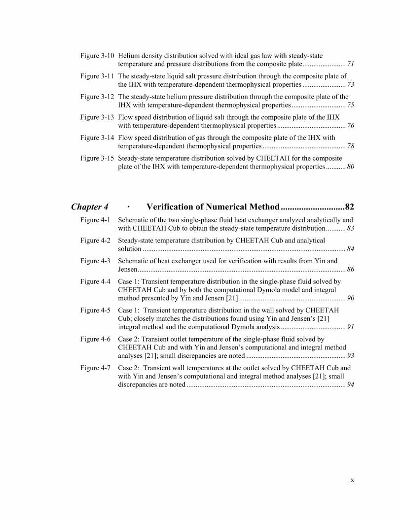
Figure 3-10 Helium density distribution solved with ideal gas law with steady-state temperature and pressure distributions from the composite plate........................ 71
Figure 3-11 The steady-state liquid salt pressure distribution through the composite plate of the IHX with temperature-dependent thermophysical properties ........................ 73
Figure 3-12 The steady-state helium pressure distribution through the composite plate of the IHX with temperature-dependent thermophysical properties .............................. 75
Figure 3-13 Flow speed distribution of liquid salt through the composite plate of the IHX with temperature-dependent thermophysical properties ...................................... 76
Figure 3-14 Flow speed distribution of gas through the composite plate of the IHX with temperature-dependent thermophysical properties .............................................. 78
Figure 3-15 Steady-state temperature distribution solved by CHEETAH for the composite plate of the IHX with temperature-dependent thermophysical properties ........... 80
Chapter 4 · Verification of Numerical Method............................82
Figure 4-1 Schematic of the two single-phase fluid heat exchanger analyzed analytically and with CHEETAH Cub to obtain the steady-state temperature distribution........... 83
Figure 4-2 Steady-state temperature distribution by CHEETAH Cub and analytical solution ................................................................................................................ 84
Figure 4-3 Schematic of heat exchanger used for verification with results from Yin and Jensen................................................................................................................... 86
Figure 4-4 Case 1: Transient temperature distribution in the single-phase fluid solved by CHEETAH Cub and by both the computational Dymola model and integral method presented by Yin and Jensen [21] ........................................................... 90
Figure 4-5 Case 1: Transient temperature distribution in the wall solved by CHEETAH Cub; closely matches the distributions found using Yin and Jensen’s [21] integral method and the computational Dymola analysis .................................... 91
Figure 4-6 Case 2: Transient outlet temperature of the single-phase fluid solved by CHEETAH Cub and with Yin and Jensen’s computational and integral method analyses [21]; small discrepancies are noted ....................................................... 93
Figure 4-7 Case 2: Transient wall temperatures at the outlet solved by CHEETAH Cub and with Yin and Jensen’s computational and integral method analyses [21]; small discrepancies are noted ........................................................................................ 94
xi
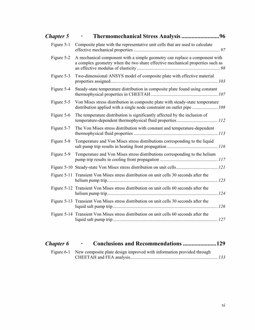
Chapter 5 · Thermomechanical Stress Analysis ..........................96 Figure 5-1 Composite plate with the representative unit cells that are used to calculate
effective mechanical properties ........................................................................... 97
Figure 5-2 A mechanical component with a simple geometry can replace a component with a complex geometry when the two share effective mechanical properties such as an effective modulus of elasticity ........................................................................ 98
Figure 5-3 Two-dimensional ANSYS model of composite plate with effective material properties assigned............................................................................................. 103
Figure 5-4 Steady-state temperature distribution in composite plate found using constant thermophysical properties in CHEETAH .......................................................... 107
Figure 5-5 Von Mises stress distribution in composite plate with steady-state temperature distribution applied with a single node constraint on outlet pipe ...................... 108
Figure 5-6 The temperature distribution is significantly affected by the inclusion of temperature-dependent thermophysical fluid properties.................................... 112
Figure 5-7 The Von Mises stress distribution with constant and temperature-dependent thermophysical fluid properties ......................................................................... 113
Figure 5-8 Temperature and Von Mises stress distributions corresponding to the liquid salt pump trip results in heating front propagation ............................................ 116
Figure 5-9 Temperature and Von Mises stress distributions corresponding to the helium pump trip results in cooling front propagation .................................................. 117
Figure 5-10 Steady-state Von Mises stress distribution on unit cells.................................... 121
Figure 5-11 Transient Von Mises stress distribution on unit cells 30 seconds after the helium pump trip................................................................................................ 123
Figure 5-12 Transient Von Mises stress distribution on unit cells 60 seconds after the helium pump trip................................................................................................ 124
Figure 5-13 Transient Von Mises stress distribution on unit cells 30 seconds after the liquid salt pump trip........................................................................................... 126
Figure 5-14 Transient Von Mises stress distribution on unit cells 60 seconds after the liquid salt pump trip........................................................................................... 127
Chapter 6 · Conclusions and Recommendations .......................129 Figure 6-1 New composite plate design improved with information provided through
CHEETAH and FEA analysis............................................................................ 133
xii
List of Tables
Chapter 5 · Thermomechanical Stress Analysis ..........................96 Table 5-1 Effective conductivities for unit cells A, B, C, and D ....................................... 102
Table 5-2 Local principle stresses on unit cells at each temperature state (MPa).............. 120
xiii
Preface
Thermal hydraulic analysis of compact heat exchangers is a well studied field.
Seminal works in this area include those by Kays, London, and Shah. In the preface to
their seminal work Compact Heat Exchangers, Kays and London briefly note the modern
history of the need for rational optimization of heat exchangers. They explain that for a
long period of time the only basic heat transfer and flow-friction design data available
was that for circular tubes. As automobiles, ships, and aircraft developed, so did the need
for heat transfer surfaces that could outperform what could be done with circular tubes.
But in order to intelligently design and specify heat exchangers with more complex and
superior heat transfer surfaces, a better understanding of existing surfaces was required.
The authors write that in the mid-to-late 1940’s the U.S. Navy Bureau of Ships and
Aeronautics, and later the Atomic Energy Commission, funded a research and testing
program to produce and publish data on the performance of many then-existing heat
exchanger surfaces. This work came in collaboration with heat exchanger manufacturers
who donated cores to their research and testing program. The manufacturers in turn
benefited from the published data and used it to improve the design of their hardware.
Similarly, increased computational capability has allowed the current generation of
engineers to characterize heat exchangers before they are built, thereby accelerating the
iterative process of design, build, test, learn, and improve. The Compact Heat Exchanger
Explicit Thermal and Hydraulics (CHEETAH) code follows in this tradition by

xiv
contributing a research tool that allows the designer to modify and improve the manifold
design of the heat exchanger in order to produce a flow distribution with increased
uniformity before the heat exchanger is built. The CHEETAH code is a research tool
that, when used in conjunction with a finite element analysis (FEA) code, allows a
designer to test the strength of a heat exchanger so that it can be designed for higher
temperatures, be built with less material, and take plants to higher efficiency than before.
After all, a fractional improvement on the power plant scale can have a very meaningful
impact.
xv
Introduction
Currently, Earth faces potentially severe environmental consequences associated with
the waste resulting from fossil fuel combustion. These energy sources fueled the
industrial revolution and an era of innovation; it is now critical that humanity develop
new sources of energy that avoid the atmospheric emissions of fossil sources. While
there are many cleaner alternatives to fossil fuels, very few of them can provide power in
a reliable and cost-effective fashion. The problem is partially related to energy flux.
Some of the most discussed alternative energy sources are wind and solar. These sources
already provide a small portion of our energy (in the United States, less than 1% total in
2009) and promise to expand significantly. However, both wind and solar power are not
only intermittent, but also relatively diffuse when compared to what is obtained from
fossil fuels. Geothermal, hydropower, and nuclear power address this issue, as these are
alternatives that could replace the base load electricity that is currently supplied by coal
and natural gas without operational atmospheric pollution.
The transportation sector, on the other hand, requires portable energy storage. This is
currently provided by fuels such as diesel, gasoline, methane, ethanol, and kerosene.
While many engineering challenges remain, hydrogen and biofuels (such as ethanol and
bio-diesel) are both being explored as possible future replacements for petroleum-based
liquid fuels. However, it is critical that any alternatives come from sources and processes
that reduce environmental externalities relative to current petroleum-based alternatives.
xvi
Additionally, battery technology is beginning to compete with the liquid fuels in the
transportation sector and may revolutionize the energy sector by allowing electric utilities
to compete with petroleum companies as energy providers for modern transportation.
One possible method to produce hydrogen is to chemically separate hydrogen from
oxygen in water via the sulfur iodine cycle. This would require an input of heat from a
very high temperature source (between 800°C and 1000°C) to be transferred to the
thermo-chemical plant. Alternatively, this heat could be used to produce electricity at
high thermodynamic efficiency. One option would be to implement a multiple reheat
helium Brayton cycle, which can provide upwards of 50% thermodynamic efficiency and
could be significantly cheaper than comparable steam turbine cycles.
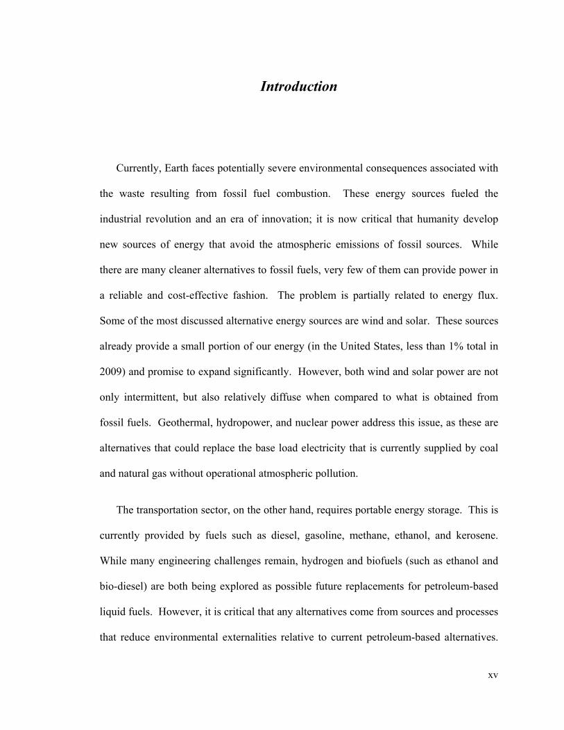
The source of this heat could be a high-temperature nuclear reactor, such as the
Advanced High-Temperature Reactor (AHTR) being researched at the University of
California, Berkeley, or a reactor such as the helium-cooled Pebble Bed Modular Reactor
(PBMR) currently under construction in South Africa. Liquid salts and inert gases such
as helium are being proposed as possible reactor coolants for various high-temperature
reactor designs. One particularly interesting design involves using an intermediate heat
transfer loop to transfer thermal energy at high temperature from a reactor to a power
plant or thermo-chemical plant located a short distance (<1km) away as illustrated
below.
xvii
Figure 0-1: Schematic of the Advanced High-Temperature Reactor joined by an
intermediate heat transfer loop (shown in red) to an adjoining power or process
plant. [Image: Prof. Per F. Peterson - UC Berkeley]
An intermediate heat exchanger (IHX) is required to transfer thermal energy from
high-temperature and high-pressure primary helium coolant to an intermediate loop. The
intermediate fluid would then transfer the thermal energy to a power plant or hydrogen
production process via another IHX near the application. In this analysis, a liquid salt is
analyzed as the intermediate coolant. This intermediate liquid, or molten, salt loop acts
as a buffer between the nuclear reactor and the hydrogen or chemical plant. This is
intrinsically beneficial for overall system safety, because by increasing the thermal inertia
in the system the intermediate loop also helps reduce the volatility of temperature
transients.
xviii
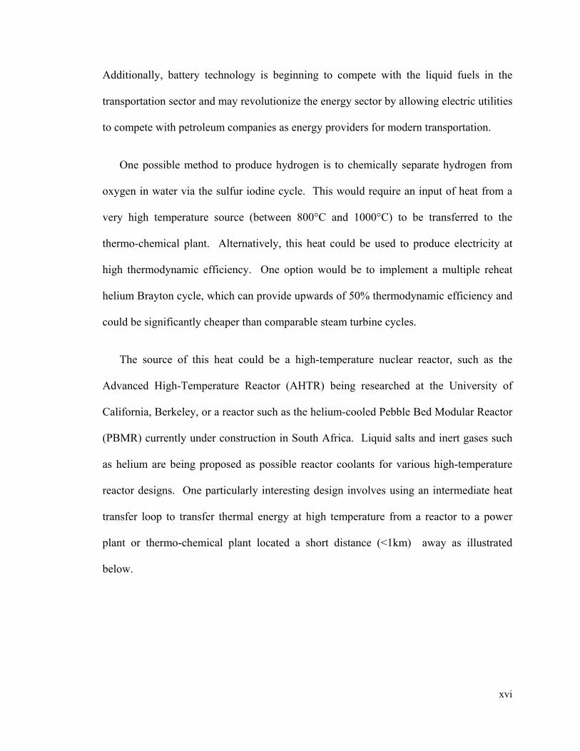
The elevated temperatures in the intermediate loop require the implementation of a
highly compact heat exchanger that retains its strength at high temperatures. Under these
conditions, plate-type heat exchangers with small flow channels are major candidates
because they can achieve high power densities with small amounts of material, and can
be fabricated using a diffusion bonding process so that the entire heat exchanger has the
strength of the base material [3]. Such a heat exchanger manufactured by Heatric is
shown in Figure 0-2.
Figure 0-2: Photo of a cut-away model of a typical Heatric plate-type compact heat
exchanger showing multiple inlet and outlet manifolds and slices across various
plates and flow channels.
xix
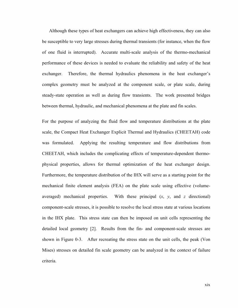
Although these types of heat exchangers can achieve high effectiveness, they can also
be susceptible to very large stresses during thermal transients (for instance, when the flow
of one fluid is interrupted). Accurate multi-scale analysis of the thermo-mechanical
performance of these devices is needed to evaluate the reliability and safety of the heat
exchanger. Therefore, the thermal hydraulics phenomena in the heat exchanger’s
complex geometry must be analyzed at the component scale, or plate scale, during
steady-state operation as well as during flow transients. The work presented bridges
between thermal, hydraulic, and mechanical phenomena at the plate and fin scales.
For the purpose of analyzing the fluid flow and temperature distributions at the plate
scale, the Compact Heat Exchanger Explicit Thermal and Hydraulics (CHEETAH) code
was formulated. Applying the resulting temperature and flow distributions from
CHEETAH, which includes the complicating effects of temperature-dependent thermo-
physical properties, allows for thermal optimization of the heat exchanger design.
Furthermore, the temperature distribution of the IHX will serve as a starting point for the
mechanical finite element analysis (FEA) on the plate scale using effective (volume-
averaged) mechanical properties. With these principal (x, y, and z directional)
component-scale stresses, it is possible to resolve the local stress state at various locations
in the IHX plate. This stress state can then be imposed on unit cells representing the
detailed local geometry [2]. Results from the fin- and component-scale stresses are
shown in Figure 0-3. After recreating the stress state on the unit cells, the peak (Von
Mises) stresses on detailed fin scale geometry can be analyzed in the context of failure
criteria.
xx
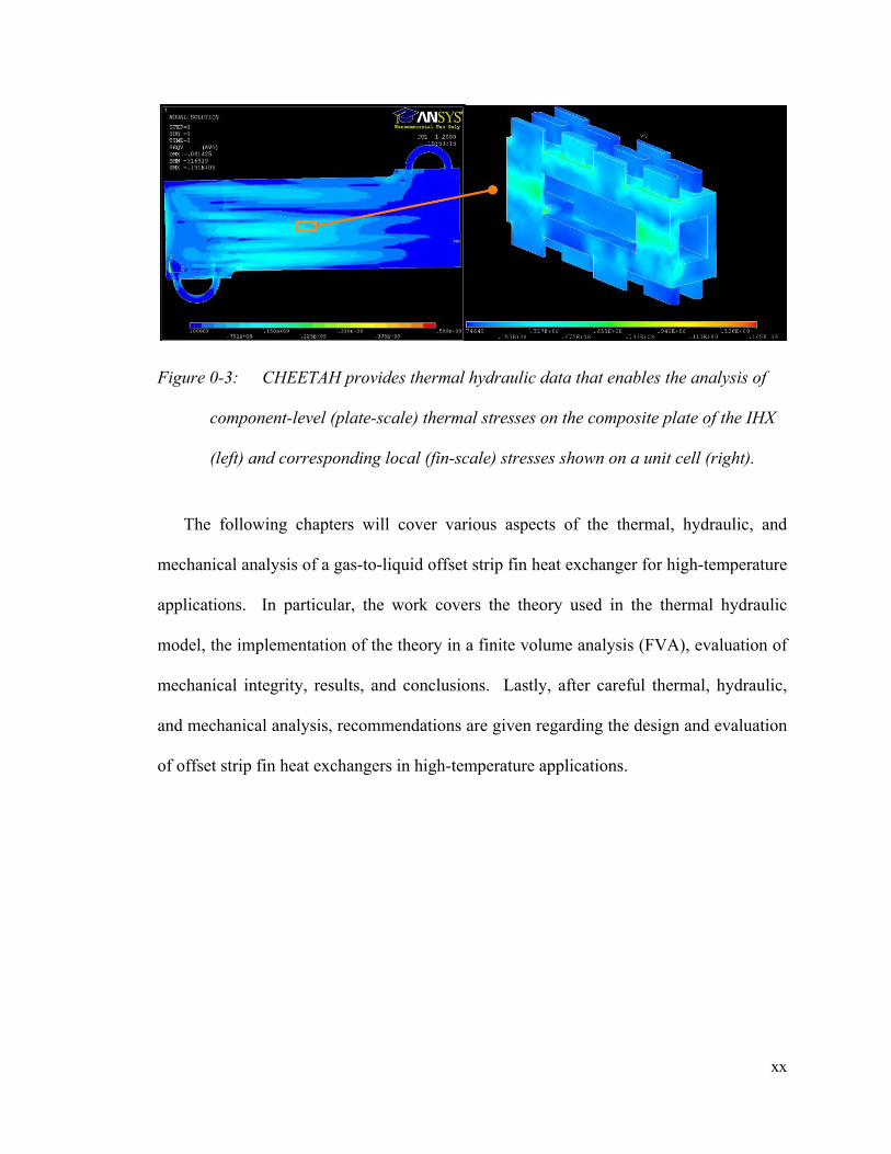
Figure 0-3: CHEETAH provides thermal hydraulic data that enables the analysis of
component-level (plate-scale) thermal stresses on the composite plate of the IHX
(left) and corresponding local (fin-scale) stresses shown on a unit cell (right).
The following chapters will cover various aspects of the thermal, hydraulic, and
mechanical analysis of a gas-to-liquid offset strip fin heat exchanger for high-temperature
applications. In particular, the work covers the theory used in the thermal hydraulic
model, the implementation of the theory in a finite volume analysis (FVA), evaluation of
mechanical integrity, results, and conclusions. Lastly, after careful thermal, hydraulic,
and mechanical analysis, recommendations are given regarding the design and evaluation
of offset strip fin heat exchangers in high-temperature applications.

xxi
Acknowledgements
I would like to acknowledge the support of my advisors, Professors Per F. Peterson
and Ralph Greif; your vision and guidance was most essential.
I am grateful for the help of Kenneth Lee for his help in performing many mechanical
stress analyses. Analyses and documentation passed on by David Huang and Dr. Hai
Hua Zhao were also instrumental in this work.
To my wife, Columba, your endless help in editing and formatting the text and also in
preparing figures made this daunting process manageable. I will always admire your
discipline, patience, and understanding; you helped me focus and finish.
I would like to recognize my brother for his example and my sister for her
perseverance and fortitude.
Most of all I would like to thank my parents for your selfless investment in your
children. Your love and encouragement were fundamental.
1
Chapter 1
Heat Exchanger Layout, Effective Porous Media (EPM) Approach,
and Conservation Equations
Compact heat exchangers achieve high heat transfer rates by employing advanced
internal geometries that increase the heat transfer surface density and create high average
convection coefficients. The offset strip fin (OSF) design is one of the most effective in
this regard because it creates a new thermal boundary layer on each fin and destroys it in
the mixed flow that occurs in its wake. Many OSF heat exchanger designs use brazing to
bond surfaces such as fins onto plates and plates onto other plates. In brazing, a material
with a lower melting point is used to fill spaces and adhere to parts made of another
material with a higher melting temperature. While this process can be employed at low
cost it significantly limits the temperature at which the brazed device can operate. For
lower temperature heat exchangers such as those used in heating, ventilation, and air
conditioning systems this may not be an issue but the lower temperature restriction of the
brazing material encumbers the application of this method in high temperature devices.
Heat exchangers with brazed joints are rarely used at temperatures over 200°C (473 K).
In high temperature applications diffusion bonded heat exchangers have the intrinsic
advantage of being made entirely of refractory alloys and thus are not being limited by a
weaker joining material. In diffusion bonding the refractory alloy plates are assembled

2
and inserted into a high temperature environment while a load is applied for an extended
period of time during which the plates fuse together. The bonded plates that make up the
heat exchanger then behave as one large cohesive part rather than as a joined assembly.
The thermal, hydraulic, and mechanical modeling of a large heat exchanger with a
complex internal geometry is challenging because important fluid dynamics, heat
transfer, and mechanical stress arise fundamentally on two scales. The thermal and
hydraulic boundary layers being created and destroyed in the fins are complex at a small
scale. The plate’s repetitive geometry of many small offset fins also creates intense
mixing which homogenizes the flow and thermal fields. This homogenizing effect
facilitates evaluation of the thermal hydraulic results on a larger scale such as that on the
component or plate level. Analysis of this system on a larger scale is similar to the
treatment of flow through a collection of small and similar particles as a collective porous
media. Using some of the same analytical tools the offset strip fin heat exchanger will be
analyzed in an effective porous media (EPM) model utilizing local volume averaged
parameters to analyze larger scale phenomena.
The EPM model is implemented computationally in the Compact Heat Exchanger
Explicit Thermal and Hydraulics (CHEETAH) code which can be used to analyze many
compact heat exchanger designs. In this work the EPM model is developed and is then
applied to a diffusion-bonded counter-flow compact intermediate heat exchanger as an
illustrative and useful example. The method and code developed can also be applied to a
parallel-flow or a cross-flow compact heat exchanger. In particular, a gas-to-liquid
intermediate heat exchanger (IHX) is analyzed as an illustrative example for the
3
methodology because it presents unique mechanical challenges associated with a large
pressure drop between the fluids and a large temperature change in the gas due to its low
volumetric heat capacity. More broadly, the system parameters in CHEETAH can be
changed to simulate other single phase fluids, flow rates, and geometries.
1.1 Intermediate Heat Exchanger Geometry
The IHX being studied is built from a diffusion-bonded stack of plates with
alternating geometry. With arrays of small offset strip fins on each side, the plates are
designed to enhance heat transfer between fluids carried in counter-flow in spaces above
and below it. In this case the heat exchanger is gas-to-liquid; when stacked, the plates
alternate between those designed to carry gas and referred to as the gas plate and the
other designed to carry liquid and referred to as the liquid plate. Furthermore, helium at 7
MPa is assumed to be the primary reactor coolant, meaning that it will be the hot fluid in
the IHX. The liquid is assumed to be a liquid or ‘molten’ salt called FLiNaK, whose
major constituents include lithium, sodium and potassium fluorides [4]. The salt has a
high volumetric heat capacity making it a very effective high-temperature heat transfer
fluid in the intermediate loop. FLiNaK is therefore the cold fluid in this intermediate heat
exchanger.
The gas and liquid plates physically separate the two fluids and enhance heat transfer
between them. Most of the heat transfer occurs in the OSF region of each plate while
most of the pressure drop occurs in the liquid plate’s pressure distribution channels
4
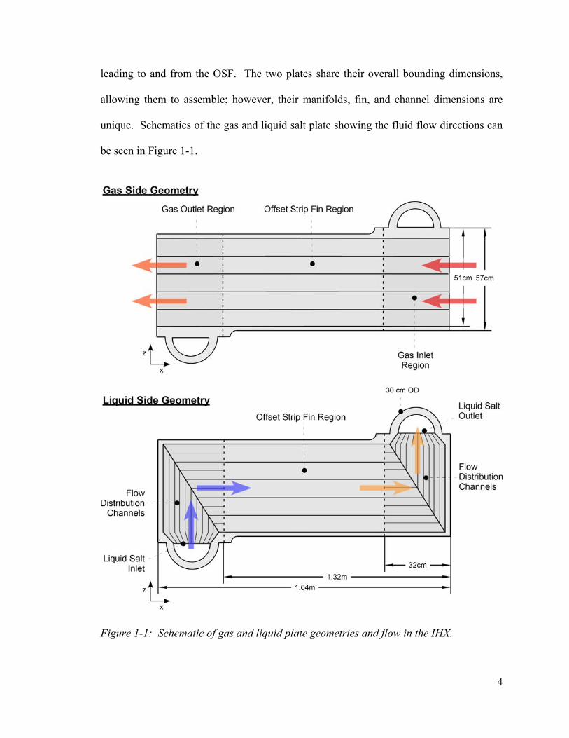
leading to and from the OSF. The two plates share their overall bounding dimensions,
allowing them to assemble; however, their manifolds, fin, and channel dimensions are
unique. Schematics of the gas and liquid salt plate showing the fluid flow directions can
be seen in Figure 1-1.
Figure 1-1: Schematic of gas and liquid plate geometries and flow in the IHX.

5
Detailed views of the manifolds and offset strip fin regions can be seen in the
isometric views from the solid models of these plates provided in Figure 1-2.
Figure 1-2: Solid models of liquid salt and helium plates in the IHX.
Detailed sizing calculations for the design of the IHX have been performed.
Initially, this analysis was done by Dr. Haihua Zhao at the University of California,
Berkeley. Later, the author of this work modified the previous analysis for slightly larger
heat exchanger dimensions to those that were currently more feasible to manufacture.
6
The complete sizing analysis is executed in a MathCad worksheet and can be found in
Appendix A.
The objective of this work lies in developing a method and associated tools to design
and improve a 50 MW heat exchanger consisting of multiple modules, testing for
viability at high temperature and with a significant (7 MPa) pressure difference between
the fluids. The heat exchanger studied here would be one of roughly 15 modules that
would make up the IHX for a 600 MW (thermal, or roughly 286 MW electric) modular
helium reactor. The device would take advantage of small fins and channels to create
hydraulic diameters that achieve high convection coefficients in the offset strip fin
regions. This is particularly useful on the liquid side where, to achieve the desired heat
transfer, the high volumetric heat capacity (ρ*cp) of the liquid salt permits very low
Reynolds number flows, low pumping power, and a moderate pressure drop along the
length of the heat exchanger.
In fact, in the manifolds and offset strip fin region of the liquid plate the slow flow of
liquid salt can be analyzed using the Darcy formulation [5,6]. Established friction factor
correlations can be used to find an effective permeability so that Darcy’s transport
equation provides a linear relationship between the mass flow rate and gradient of the
flow potential. The constant in this linear relation is called the hydraulic conductivity in
groundwater hydrology because the equation is analogous to Fourier’s law for
conduction. This hydraulic conductivity is a function of the effective permeability,
viscosity and density of the fluid. In the gas flow region the flow has Reynolds numbers
is in the hundreds meaning that the regime is not Darcian. However, by knowing the

7
steady state flow rates, density, and viscosity, an effective permeability can be calculated
using a technique presented later when the volume averaged effective permeability of the
media is presented.
1.2 Volume-Averaged Properties
One of the main advantages of the effective porous media (EPM) model being
presented here is the ability to focus on component scale flow distribution, pressure
losses, and heat transfer via volume averaging. This allows the user to pursue solutions
at the scale of the composite plate, using information from previous work that focused on
the local scale or fin scale phenomena. It is critical that the correlations used to find
volume-averaged properties be used within their established range of validity.
Correlations are chosen based on average flow rates calculated from general sizing
calculations for the heat exchanger that can be found in Appendix A. This approach
allows the user to avoid having to discretize and analyze flow and heat transfer
simultaneously at both the largest and smallest geometric scales, something that would
require a prohibitive grid resolution.
A more detailed analysis on the fin scale would involve looking at phenomena in the
periodic thermal-boundary layers created in the interrupted flow by the offset strip fins.
This type of analysis could focus on the flow through a single channel over a row of fins.
In this scenario, the variation of the convection coefficient over the length of the fin row
could be examined. The fluid temperature profile as a function of distance beginning at
8
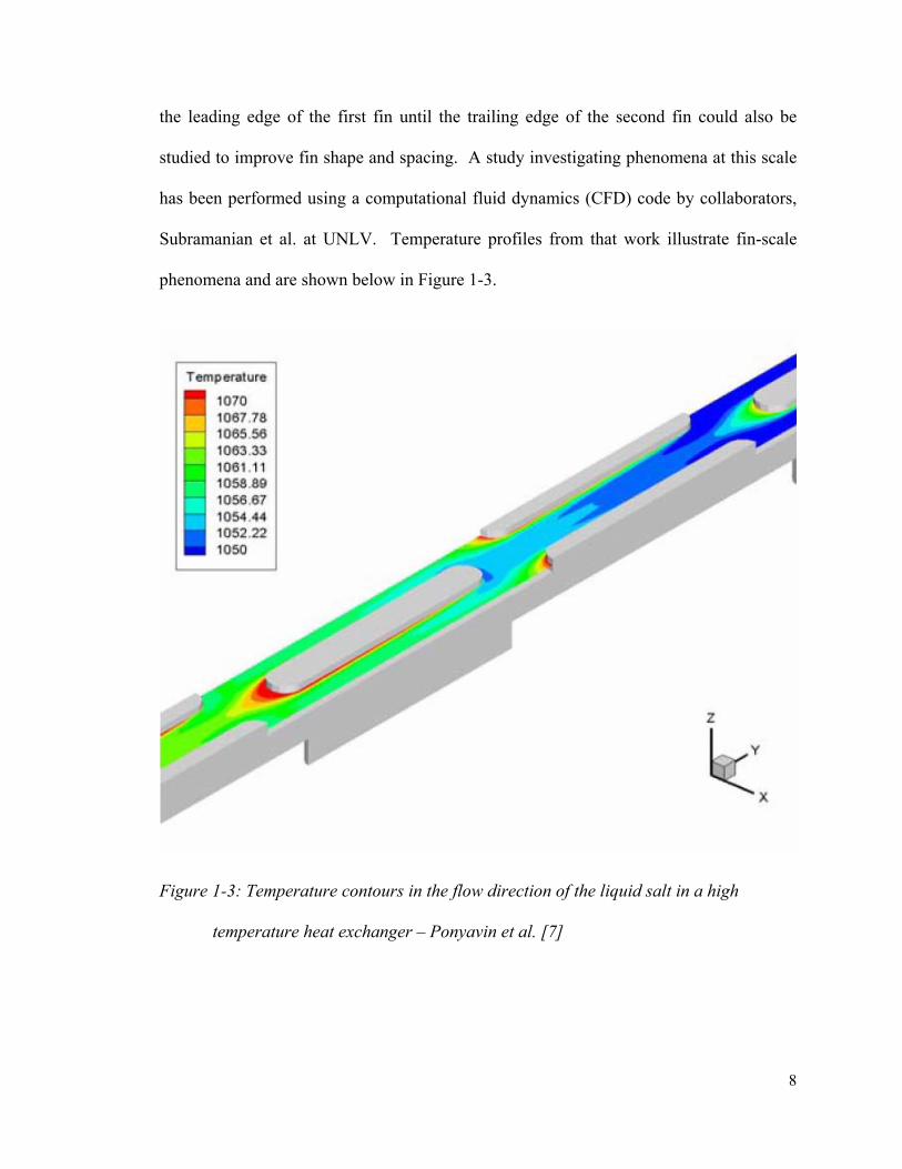
the leading edge of the first fin until the trailing edge of the second fin could also be
studied to improve fin shape and spacing. A study investigating phenomena at this scale
has been performed using a computational fluid dynamics (CFD) code by collaborators,
Subramanian et al. at UNLV. Temperature profiles from that work illustrate fin-scale
phenomena and are shown below in Figure 1-3.
Figure 1-3: Temperature contours in the flow direction of the liquid salt in a high
temperature heat exchanger – Ponyavin et al. [7]
9
In the case shown above, the temperature variation over the set of fins is the matter
of interest, as it aids in understanding fin scale phenomena. Hu and Herold have also
published work examining the effects of Prandtl number on pressure drop, on heat
transfer and on the length of the developing region [8].
However, the primary interest in this work involves thermal analysis on the heat
exchanger module level, in order to determine thermal expansion and stresses under
steady state and transient conditions. These phenomena will not be dominated by what
happens at the fin scale, but rather by the large temperature variation over a long and flat
plate-type offset strip fin heat exchanger plate. It is important to point out that examining
this plate at the fin scale would be computationally prohibitive. Instead, at the system
scale one focuses on system scale phenomena and uses Nusselt correlations evaluated
from well established experimental sources for these geometries.
These heat transfer correlations are well documented in classic sources such as Kays
and London [9]. For the case of interest here, a correlation submitted by Manglik and
Bergles [10] fits for the offset strip fin heat exchanger arrangement and range of
Reynolds numbers. This work by Manglik and Bergles is a good overview of work done
on the offset strip fin geometry. It includes results published by Kays and London, Joshi
and Webb, Weiting, Manson, and Mochizuki et al. Applying Nusselt numbers rooted in
correlations defined for periodic fully-developed flow such as those by Manglik and
Bergles allows the EPM model to discretize with a significantly coarser grid (100 times
coarser than would be used in a traditional analysis using CFD). Since decreasing the
grid size causes a quadratic increase in the number of computations required, increasing
10
the grid size greatly reduces the computational resources required to analyze transient
behavior in a large and complex heat exchanger module.
In the thermal hydraulic model there are many local volume-averaged properties that
are important. These properties include the hydraulic diameter Dh, phase fraction φ ,
medium permeability, k, surface area density, and the convective heat transfer coefficient,
h. With the exception of the temperature dependent fluid properties, all of the above
mentioned local volume-averaged properties are geometry specific. This means that it is
the local detailed geometry of the plates that determines these local volume averages.
In order to calculate local volume averages, it is important to first specify the
medium in which these properties will be defined. In this case, the medium will be the
‘composite plate’. Because the liquid and gas plates form an alternating stack, it is
logical to treat the assembly of a gas and liquid plate as a uniform and repeating
geometry. But if this assembly of the gas and liquid plate is used, an opportunity to
achieve mechanical symmetry is lost. Since the composite plate geometry does provide
mechanical symmetry it is used instead to define unit cells. This mechanical symmetry
will become important later in the mechanical stress analysis. More importantly, by
selecting this composite plate instead of the simple gas and liquid plate assembly, a
repeating geometry is selected that is also symmetric on more planes. This technique
simplifies the thermal hydraulic analysis. The selection of the composite plate from the
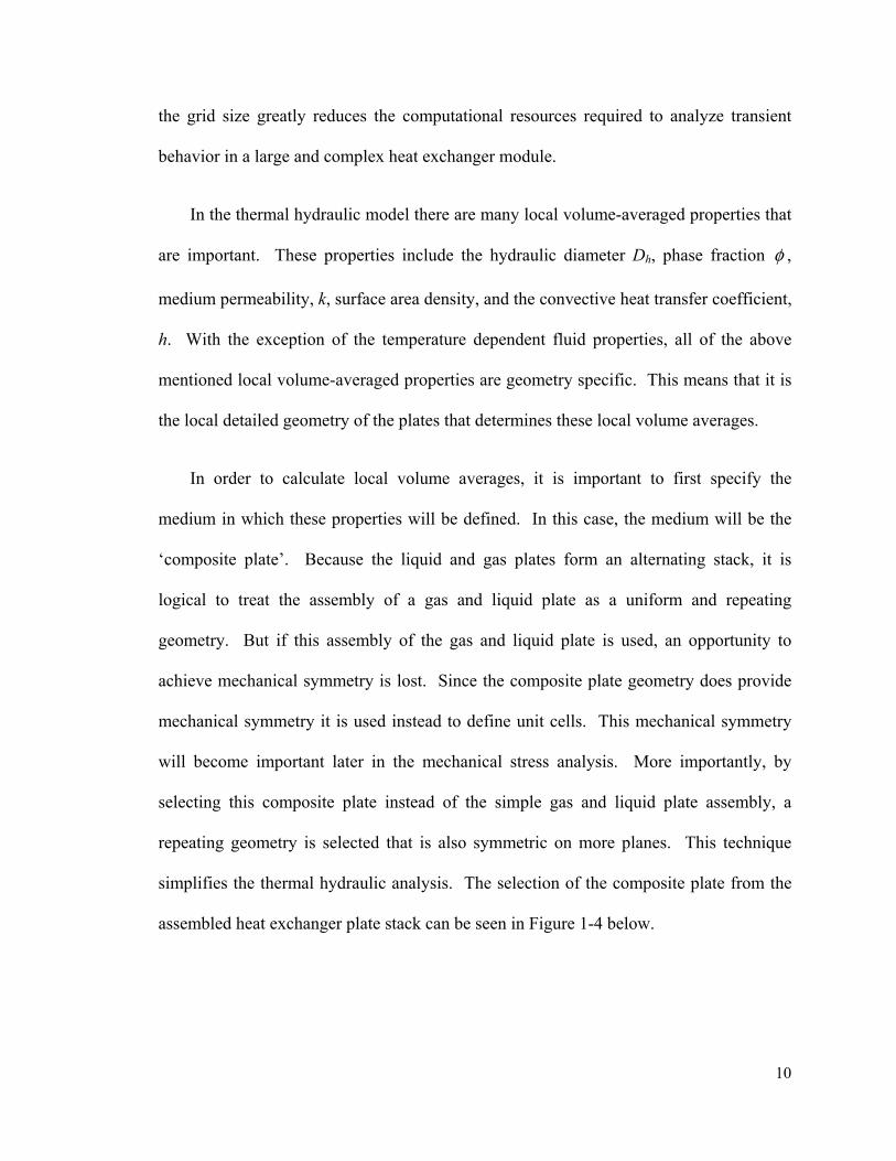
assembled heat exchanger plate stack can be seen in Figure 1-4 below.
11
Figure 1-4: Cut-away view through the offset strip fin (OSF) section showing alternating
liquid and gas flow channels. Dark bands at the top of each fin indicate the
location of diffusion-bonded joints between the plates.
From the top view, this composite plate can be analyzed as having four
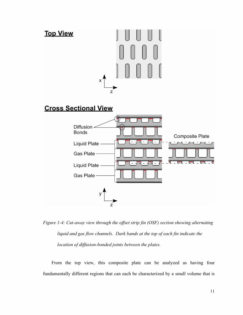
fundamentally different regions that can each be characterized by a small volume that is
12
repeated to yield the entire region. That characteristic volume will be referred to as the
unit cell for that region and each unit cell will be analyzed for several pertinent volume-
averaged properties. The four unit cells that make up the composite plate are shown in
Figure 1-5.
Figure 1-5: The four unit cells characterizing the complex geometry of the composite
plate.

13
1.3 Phase Fraction
The phase fraction represents the ratio of the volume of a particular phase to the
volume denoted by the largest dimensions of each unit cell in each of the principal
directions. In Figure 1-6 below, the volume of the solid phase in unit cell C is shown on
the left, while the volume of the box needed to contain it is shown bordered in red to the
right. The ratio of solid phase volume to the box volume is referred to as the phase
fraction. This is a local volume-averaged property within the zone of the IHX where unit
cell C describes the local geometry.
Figure 1-6: Solid phase fraction illustration for unit cell C (67%).

14
1.4 Media Permeability
The medium permeability is also obtained via a local volume average. Extensive
analytical and experimental work has been done to characterize the heat transfer
properties of many offset strip fin geometries. Kays and London, Shah, Webb and others
have published a large body of correlations for the heat transfer characteristics of heat
exchangers. Kays and London in particular published many correlations specifically for
compact heat exchangers. While this subject is of great importance it is also one of great
complexity because the phenomena influencing the fluid mechanics and heat transfer
vary with fin geometry, flow regime, and with manufacturing methods used in making
the fins for the compact heat exchanger.
Many correlations exist for widely varying conditions. Most often, however, the
Fanning friction factor is used to quantify the pressure losses due to friction in the flow.
The correlations for the Fanning friction factor very often have the following form:
1 Recff C∝ i
Equation 1-1
where C1 is a function of various parameters relevant to the fin and channel
geometry and c is an empirical constant. Since these correlations are developed for flow
over the length of an offset strip fin channel, the friction factor is a volume average over
the entire length, width, and height of the flow path. This Fanning friction factor then
allows the researcher to determine the permeability of the medium via a method
explained in following section.
15
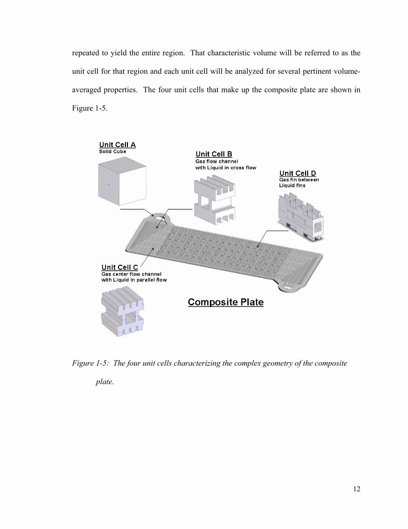
1.5 Determining the Effective Permeability
For one-dimensional, fully developed steady state laminar flow in a pipe, the axial
component of the momentum equation can be solved for the average axial (x-direction)
velocity u shown in Equation 1-2 [11].
2
32D du
dxμ− Φ= or
22 * Re
32 32D d D du u
dx dxμ ρ− Φ Φ= = − Equation 1-2
Here it can be clearly seen that 2
32D serves as the geometry-dependent correction
factor similar to the permeability, which has the same units.
This is also commonly expressed as:
2
2 f
D duf dxρ
Φ= − Equation 1-3
whereby the Fanning friction factor for laminar flow in a pipe is thus
16Reff =
Equation 1-4
Now dividing Equation 1-3 by the average fluid velocity gives the following
equation for flow in a pipe.
12 f
D duf u dx
μρ μ
Φ= − Equation 1-5

16
Applying this to the effective porous medium for laminar, fully developed steady
state flow, the diameter D is replaced by the hydraulic diameter Dh and the average
velocity is represented as u (average velocity in a pipe or analogous to the interstitial
velocity in the effective porous medium). The Darcy velocity uD is the interstitial
velocity divided by the phase fraction, φ , (conventionally referred to as the porosity), as
follows:
intDuu u
φ= = Equation 1-6
Thus Equation 1-5 becomes
2 12
h xD
f D
D duf u dx
μφρ μ
Φ= − Equation 1-7
This finally determines the relationship between the Fanning friction factor and the
effective permeability as:
2
2h
xf D
Dkf u
μφρ
= Equation 1-8
Because the Fanning friction factor and thus the permeability are function of fluid
velocity (especially at higher Reynolds numbers) the average velocity of the fluid flow
must be known in order to calculate the permeability. In this case, the average velocity
comes from mass flow rates determined from component sizing calculations that can be
found in Appendix A. With the permeability known, the velocities at the fin-scale can be
17
calculated. An array of fin-scale velocities forms a velocity field inside of the heat
exchanger.
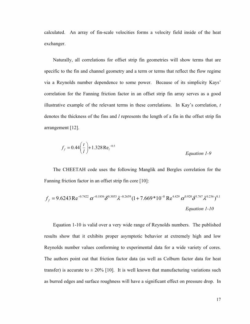
Naturally, all correlations for offset strip fin geometries will show terms that are
specific to the fin and channel geometry and a term or terms that reflect the flow regime
via a Reynolds number dependence to some power. Because of its simplicity Kays’
correlation for the Fanning friction factor in an offset strip fin array serves as a good
illustrative example of the relevant terms in these correlations. In Kay’s correlation, t
denotes the thickness of the fins and l represents the length of a fin in the offset strip fin
arrangement [12].
0.50.44 1.328Ref ltfl
−⎛ ⎞= +⎜ ⎟⎝ ⎠ Equation 1-9
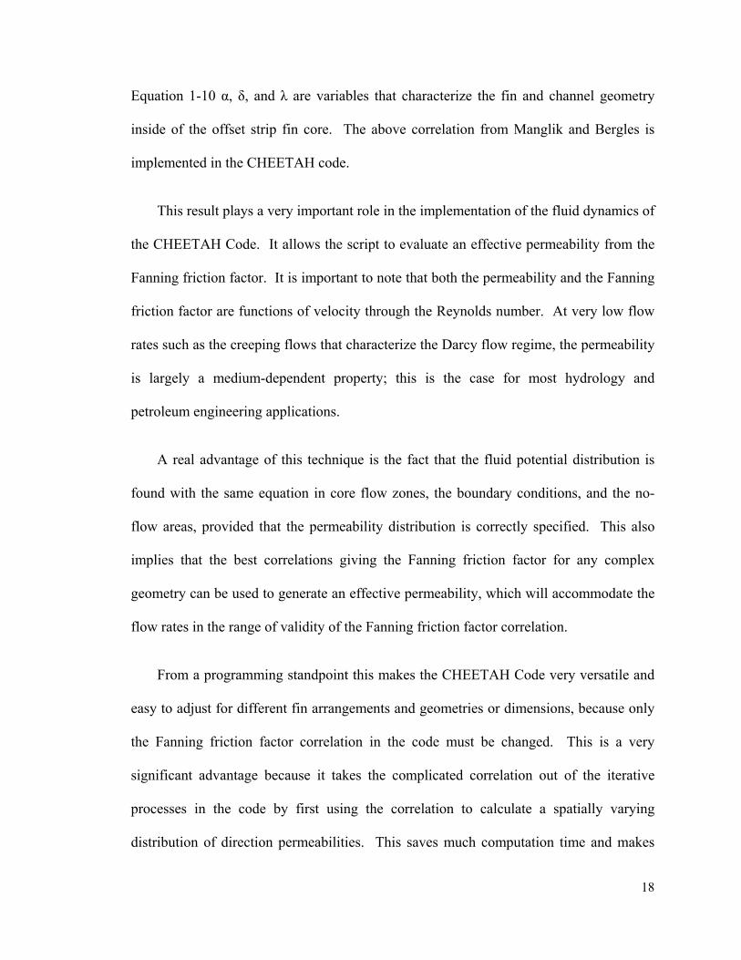
The CHEETAH code uses the following Manglik and Bergles correlation for the
Fanning friction factor in an offset strip fin core [10]:
0.7422 0.1856 0.3053 0.2659 8 4.429 0.920 3.767 0.236 0.19.6243Re (1 7.669*10 Re )ff α δ λ α δ λ− − − −= +
Equation 1-10
Equation 1-10 is valid over a very wide range of Reynolds numbers. The published
results show that it exhibits proper asymptotic behavior at extremely high and low
Reynolds number values conforming to experimental data for a wide variety of cores.
The authors point out that friction factor data (as well as Colburn factor data for heat
transfer) is accurate to ± 20% [10]. It is well known that manufacturing variations such
as burred edges and surface roughness will have a significant effect on pressure drop. In
18
Equation 1-10 α, δ, and λ are variables that characterize the fin and channel geometry
inside of the offset strip fin core. The above correlation from Manglik and Bergles is
implemented in the CHEETAH code.
This result plays a very important role in the implementation of the fluid dynamics of
the CHEETAH Code. It allows the script to evaluate an effective permeability from the
Fanning friction factor. It is important to note that both the permeability and the Fanning
friction factor are functions of velocity through the Reynolds number. At very low flow
rates such as the creeping flows that characterize the Darcy flow regime, the permeability
is largely a medium-dependent property; this is the case for most hydrology and
petroleum engineering applications.
A real advantage of this technique is the fact that the fluid potential distribution is
found with the same equation in core flow zones, the boundary conditions, and the no-
flow areas, provided that the permeability distribution is correctly specified. This also
implies that the best correlations giving the Fanning friction factor for any complex
geometry can be used to generate an effective permeability, which will accommodate the
flow rates in the range of validity of the Fanning friction factor correlation.
From a programming standpoint this makes the CHEETAH Code very versatile and
easy to adjust for different fin arrangements and geometries or dimensions, because only
the Fanning friction factor correlation in the code must be changed. This is a very
significant advantage because it takes the complicated correlation out of the iterative
processes in the code by first using the correlation to calculate a spatially varying
distribution of direction permeabilities. This saves much computation time and makes
19
the effective porous media (EPM) treatment advantageous. For some heat transfer
surface geometries tested correlations may not exist. For such cases it would be
necessary measure flow resistance experimentally and use these measurements to
establish the effective permeability.
1.6 Fully Developed Flow
For this approach, it is important to show that the flow has reached a hydro-
dynamically fully developed condition. The offset fin studies of Hu and Harold, Sparrow
et al, and Kelkar and Patankar show that for Graetz number, Gz<200 the flow has
effectively reached a periodic hydrodynamic fully developed condition [8, 13, 14].
Re* hDGzx
= Equation 1-11
For the IHX being analyzed here, on the liquid-side the Reynolds number varies
between 20 and 50 with a hydraulic diameter near 4 mm. This makes the hydro-dynamic
entry length is just a fraction of a millimeter on a 1 meter core section making it less than
1% of the core length on the fluid side. Similarly, on the gas-side of the IHX the
Reynolds number is near 2600 with a hydraulic diameter of 6 mm. The hydrodynamic
entry length is therefore larger on the gas plate at around 6.0 cm in length or 6% of the
core length on the gas side. In this analysis for both cases the flow is treated entirely as
fully developed.
20
1.7 Convection Coefficient
Offset strip fins are widely used due to their compact nature and high effectiveness
in enhancing heat transfer. The enhancement to heat transfer stems from the periodic
starting of a new boundary layer on each fin and its subsequent elimination in the wake
following the fin. The fin spacing is most often uniform with roughly half-fin spacing in
between fins [10]. Manufacturing processes can also influence heat transfer enhancement
by producing burred edges and affecting surface roughness. The heat transfer
enhancement comes with increased pressure drop as the finite fin thickness produces
form drag and enhanced viscous shear.
The Colburn factor, j, is related to the Nusselt number as follows:
2 13 3Pr /(Re Pr )j Co St Nu= = ⋅ = ⋅ Equation 1-12
Or
13(Re Pr )Nu j= ⋅ ⋅ Equation 1-13
and therefore
13(Re Pr ) f
h
kh j
D= ⋅ ⋅
Equation 1-14
21
As an illustrative example of a simple correlation for the Colburn factor, j, Kays used
the following correlation for a laminar boundary layer over an interrupted plate geometry.
0.50.665Relj −= Equation 1-15
The Colburn factor is a function of fluid velocity; in order to specify the convection
coefficient distribution in the CHEETAH code, the average velocities were initially used.
These velocities came from mass flow rates determined from component sizing
calculations that can be found in Appendix A. Later versions of the code use velocities
solved at the fin-scale to calculate local Reynolds numbers from which the convection
coefficients are calculated at the fin-scale.
As with the Fanning friction factor, in the offset strip fin region the CHEETAH code
uses a more complicated Colburn factor correlation by Manglik and Bergles (Equation
1-16) that is valid over a large range of Reynolds numbers and includes the correct
asymptotic behavior. The authors point out that the Colburn factor data are accurate to
±20% due to variability of many relevant factors including surface roughness and
manufacturing methods [10].
0.5403 0.1541 0.1499 0.0678 5 1.340 0.504 0.456 1.055 0.10.6522 Re (1 5.269*10 Re )j α δ λ α δ λ− − − − −= +
Equation 1-16
22
1.8 Surface Area Density
Finding the surface area density of each unit cell is straight forward. It involves
finding the ratio of the surface area in contact with the liquid and dividing by the volume
found by multiplying the largest dimensions of each unit cell in each of the principal
directions. More concisely, it is the surface area in contact with the fluid divided by the
volume of the box needed to enclose the unit cell (see Figure 1-6). A surface area density
exists for each fluid and each unit cell.
1.9 Effective Conductivity
Due to the stacked assembly, the flow areas on the liquid and gas plates overlap in
many regions of the composite plate creating zones in the solid material with complex
geometry and complex mechanical and thermal unit-cell properties. One of these
properties is the directional conductivity in each unit cell that makes up the composite
plate seen in Figure 1-5. In order to find the directional conductivity of each of these unit
cells, the conductivity of the material is inserted into a FEA code. In this case both
ANSYS and COMSOL were used. With the material conductivity specified, a
temperature is imposed on opposite planes of the unit cell and the FEA is then able to
find the steady state temperature gradient through the material. Clearly some areas will
be thicker than others and will thus have a lower effective conductivity. The FEA code
can readily solve for the conduction heat transfer through the complex geometry of the
solid material in the unit cell. This heat transfer rate, divided by the area of the entire
23
face (not just the solid fraction) will give the effective conductivity of the unit cell in that
direction.
1.10 Fluid Dynamics
Initially, thermophysical constants such as density and viscosity were treated as
constants to facilitate the creation of the initial thermal hydraulic model presented here.
In later versions of the model these properties were made temperature-dependent to
increase accuracy. Including the temperature-dependent thermophysical properties better
reflects flow maldistribution phenomena that would result from complex temperature
distributions in the heat exchanger. This was particularly important when investigating
the feasibility of gas-cooled reactors, because the relatively low volumetric heat capacity
(relative to liquid-cooled reactors) of the gases requires both high volumetric flow rates
and results in considerable changes in temperature from inlet to outlet for a given heat
input.
1.11 Fluid Dynamics Equations
In all cases involving steady flow, mass must be conserved in any representative
control volume in the field of flow along a plate. Two-dimensional mass conservation
can be expressed in the equation of continuity while assuming constant density in both
fluids as follows:
24
0u wx z
∂ ∂+ =∂ ∂ Equation 1-17
Darcy’s transport equation serves as a modified momentum equation relating
pressure gradients to fluid velocities. The effective permeability, kx and kz are functions
of the geometry and Reynolds numbers.
Darcy’s transport equation for one-dimensional flow in porous media is:
intx
D xk g dhu u
dxρφμ
= ⋅ = − or xD
k dudxμΦ= − Equation 1-18
intz
D zk g dhw w
dzρφμ
= ⋅ = − or zD
k dwdzμΦ= − Equation 1-19
Here, Φ is the flow potential (Pa) and u is the Darcy velocity such that Φ= P+ρgz.
More information on the application of Darcy’s transport equations to porous media can
be found in references by Peaceman [5] and Domenico [3].
In order to find the velocity distribution in the IHX it is necessary to first find the
pressure distribution. The following equation shows one way to accomplish this.
Due to spatially-varying viscosity μ and permeability k (density is assumed
constant), the partial derivative of the x and z components of the fluid velocity gives:
2
2 2
1Ddu dk d k d k ddx dx dx dx x dx
μμ μ μ
Φ ∂Φ Φ= − + −∂
Equation 1-20
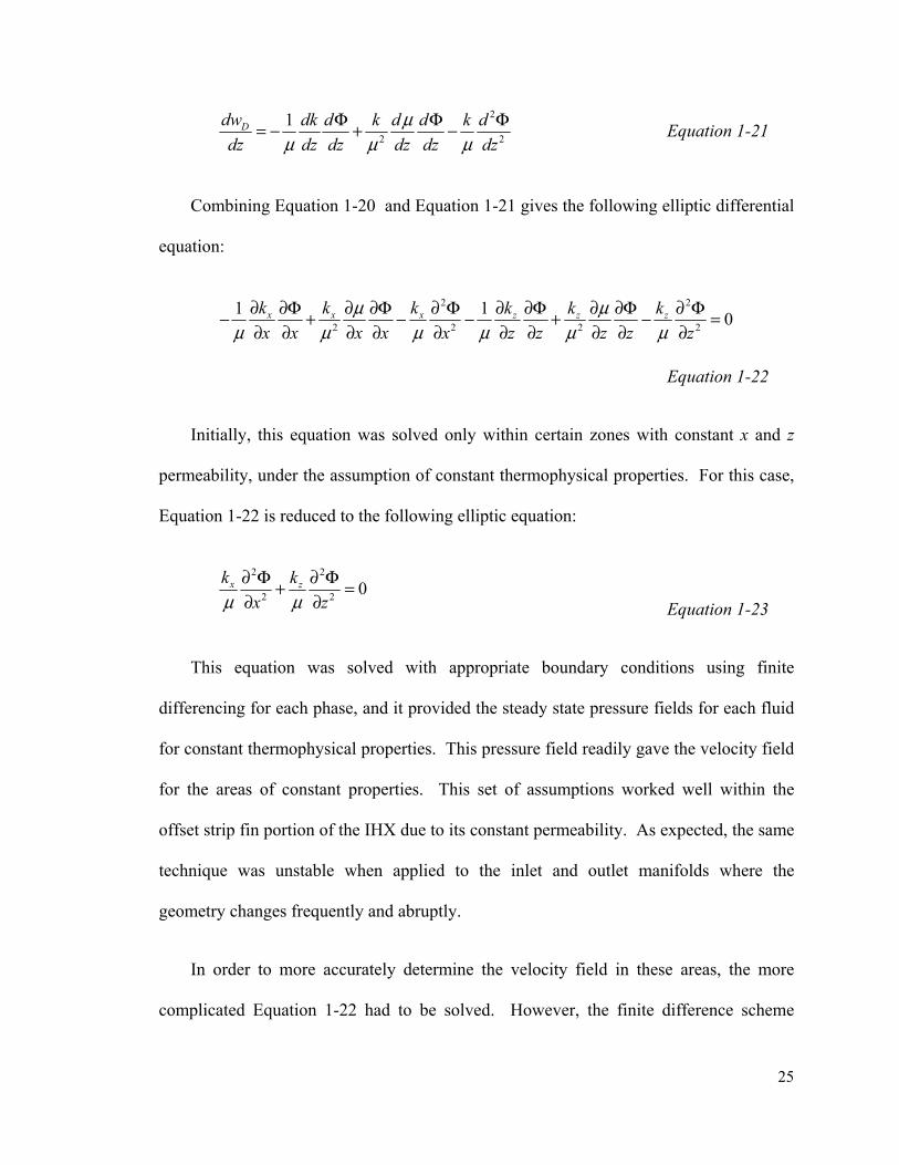
25
2
2 2
1Ddw dk d k d d k ddz dz dz dz dz dz
μμ μ μ
Φ Φ Φ= − + − Equation 1-21
Combining Equation 1-20 and Equation 1-21 gives the following elliptic differential
equation:
2 2
2 2 2 2
1 1 0x x x z z zk k k k k kx x x x x z z z z z
μ μμ μ μ μ μ μ
∂ ∂∂Φ ∂ ∂Φ ∂ Φ ∂Φ ∂ ∂Φ ∂ Φ− + − − + − =∂ ∂ ∂ ∂ ∂ ∂ ∂ ∂ ∂ ∂
Equation 1-22
Initially, this equation was solved only within certain zones with constant x and z
permeability, under the assumption of constant thermophysical properties. For this case,
Equation 1-22 is reduced to the following elliptic equation:
2 2
2 2 0x zk kx zμ μ
∂ Φ ∂ Φ+ =∂ ∂ Equation 1-23
This equation was solved with appropriate boundary conditions using finite
differencing for each phase, and it provided the steady state pressure fields for each fluid
for constant thermophysical properties. This pressure field readily gave the velocity field
for the areas of constant properties. This set of assumptions worked well within the
offset strip fin portion of the IHX due to its constant permeability. As expected, the same
technique was unstable when applied to the inlet and outlet manifolds where the
geometry changes frequently and abruptly.
In order to more accurately determine the velocity field in these areas, the more
complicated Equation 1-22 had to be solved. However, the finite difference scheme
26
resulted in large instabilities in the zones where the permeability varies from node to
node such as in the diffuser, reducer, and at the interface between two zones of different
permeability, such as between the OSF region and the inlet and outlet manifolds. The
instabilities arose from the first derivatives of permeability with respect to space, xkx
∂∂
and zkz
∂∂
because these values are undefined at the interface between two zones where
there is a step change in the permeability.
This instability was overcome by using a finite volume analysis (FVA), commonly
called the control volume approach. In this approach, the conservation equations are
applied over a discrete area, volume, or grid from the outset. The velocities are obtained
from the pressure relationships given in Darcy’s transport equation. The FVA or control
volume formulation involves performing a mass, momentum, and energy balance on a
volume of predetermined size. Unlike the Taylor-series based approaches in the finite
difference formulation, the FVA does not take the limit by reducing the control volume
down to a point (differential region) but rather to a predetermined size [15]. This
provides a significantly more stable solution that can tolerate step changes in
conductivity, permeability, viscosity, and pressure since the conservation equation is
asserted on each discrete area or volume in the grid over the discretized time. Of course,
for explicit solutions certain stability criteria must be obeyed, such as the Fourier and
Courant numbers; which are discussed in the following chapter.
27
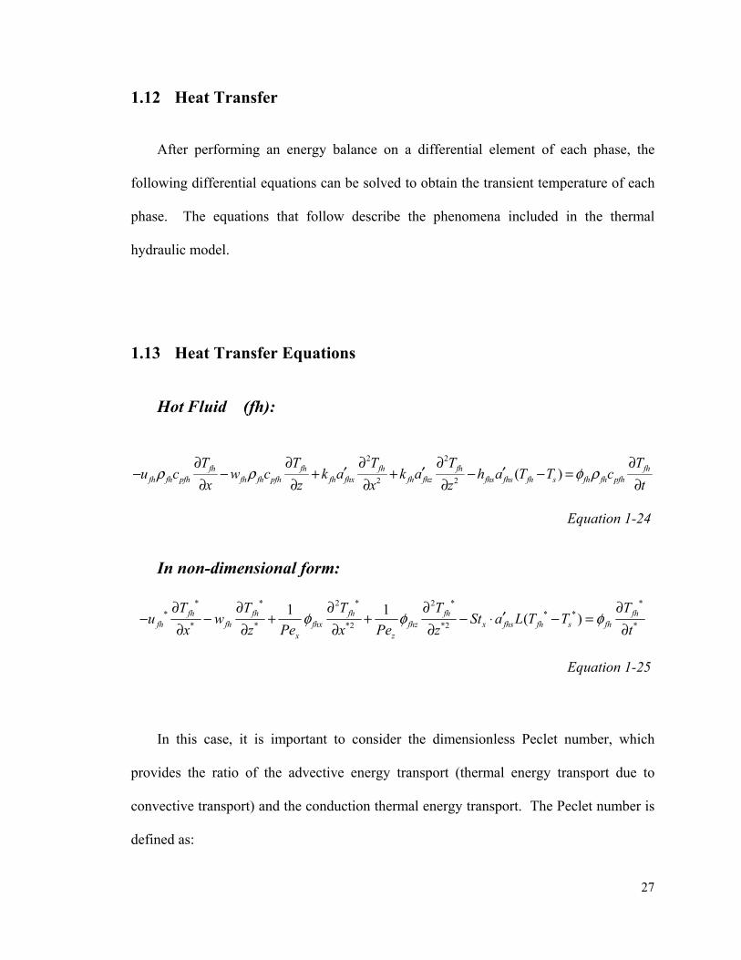
1.12 Heat Transfer
After performing an energy balance on a differential element of each phase, the
following differential equations can be solved to obtain the transient temperature of each
phase. The equations that follow describe the phenomena included in the thermal
hydraulic model.
1.13 Heat Transfer Equations
Hot Fluid (fh):
2 2
2 2 ( )fh fh fh fh fhfh fh pfh fh fh pfh fh fhx fh fhz fhs fhs fh s fh fh pfh
T T T T Tu c w c k a k a h a T T c
x z x z tρ ρ φ ρ
∂ ∂ ∂ ∂ ∂′ ′ ′− − + + − − =
∂ ∂ ∂ ∂ ∂ Equation 1-24
In non-dimensional form:
* * 2 * 2 * ** * *
* * *2 *2 *
1 1 ( )fh fh fh fh fhfh fh fhx fhz x fhs fh s fh
x z
T T T T Tu w St a L T T
x z Pe x Pe z tφ φ φ
∂ ∂ ∂ ∂ ∂′− − + + − ⋅ − =
∂ ∂ ∂ ∂ ∂
Equation 1-25
In this case, it is important to consider the dimensionless Peclet number, which
provides the ratio of the advective energy transport (thermal energy transport due to
convective transport) and the conduction thermal energy transport. The Peclet number is
defined as:

28
* * ** pu x cu xPek
ρα
ΔΔ= = Equation 1-26
The Peclet number for the helium flow is approximately 500, while the Peclet
number for the liquid salt flow in the composite plate is near 165. In both cases, this
means that the energy balance is dominated by the advective contribution to the point that
the conductive contribution in the flow direction can be ignored with a negligible effect
on accuracy.
Neglecting conduction in the hot fluid the energy balance is reduced to:
( )fh fh fhfh fh pfh fh fh pfh fhs fhs fh s fh fh pfh
T T Tu c w c h a T T c
x z tρ ρ φ ρ
∂ ∂ ∂′− − − − =
∂ ∂ ∂
Equation 1-27
Solid (s):
2 2
2 2( ) ( ) s s sfhs fhs fh s sfc sfc s fc s k s k s s ps
T T Th a T T h a T T k a k a cx z t
φ ρ∂ ∂ ∂′ ′ ′ ′− − − + + =∂ ∂ ∂
Equation 1-28
In non-dimensional form:
2 * 2 * ** * * *
*2 *2 *( ) ( )fc fc sx fhx z fhz x fcs fh s x fcs s fc s
T T TFo Fo St a L T T St a L T Tx z t
φ φ φ∂ ∂ ∂′ ′⋅ − ⋅ + ⋅ − − ⋅ − =∂ ∂ ∂
Equation 1-29
29
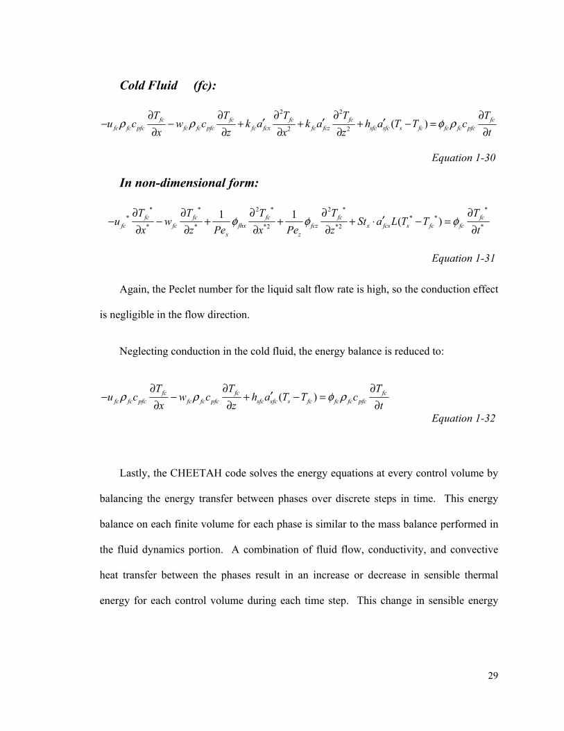
Cold Fluid (fc):
2 2
2 2 ( )fc fc fc fc fcfc fc pfc fc fc pfc fc fcx fc fcz sfc sfc s fc fc fc pfc
T T T T Tu c w c k a k a h a T T c
x z x z tρ ρ φ ρ
∂ ∂ ∂ ∂ ∂′ ′ ′− − + + + − =
∂ ∂ ∂ ∂ ∂ Equation 1-30
In non-dimensional form:
* * 2 * 2 * ** * *
* * *2 *2 *
1 1 ( )fc fc fc fc fcfc fc fhx fcz x fcs s fc fc
x z
T T T T Tu w St a L T T
x z Pe x Pe z tφ φ φ
∂ ∂ ∂ ∂ ∂′− − + + + ⋅ − =
∂ ∂ ∂ ∂ ∂
Equation 1-31
Again, the Peclet number for the liquid salt flow rate is high, so the conduction effect
is negligible in the flow direction.
Neglecting conduction in the cold fluid, the energy balance is reduced to:
( )fc fc fcfc fc pfc fc fc pfc sfc sfc s fc fc fc pfc
T T Tu c w c h a T T c
x z tρ ρ φ ρ
∂ ∂ ∂′− − + − =
∂ ∂ ∂ Equation 1-32
Lastly, the CHEETAH code solves the energy equations at every control volume by
balancing the energy transfer between phases over discrete steps in time. This energy
balance on each finite volume for each phase is similar to the mass balance performed in
the fluid dynamics portion. A combination of fluid flow, conductivity, and convective
heat transfer between the phases result in an increase or decrease in sensible thermal
energy for each control volume during each time step. This change in sensible energy
30
manifests itself as a change in temperature of the finite volume for each phase. These
energy balances are analyzed in greater detail in the following chapter.
1.14 Temperature-Dependent Fluid Properties
Solving for the fluid flow and temperature distribution using temperature-dependent
thermophysical properties is particularly important for this case because of the large
change in temperature in the fluids. Furthermore, the primary coolant (helium at 7 MPa
for this reactor design) in particular experiences a large temperature change in the heat
exchanger, because like all gases it has a volumetric heat capacity that is low compared to
that of liquids. Among the thermophysical properties of both fluids, viscosity is by far
the most sensitive to changes in temperature; however, the density of the helium also
varies considerably over this large temperature change.
In this case, analyses are conducted using both constant and variable thermophysical
properties; the temperature distribution found with constant thermophysical properties is
used as the initial condition for the analysis using variable thermophysical properties.
This initial temperature distribution is critical because it will determine the initial
viscosity distribution, which will in turn allow the determination of the mass flow
distribution after solving the equations presented in the previous section on fluid
mechanics. Because it would be computationally expensive to calculate viscosity and
density distributions for every time step, CHEETAH allows the user to adjust the time
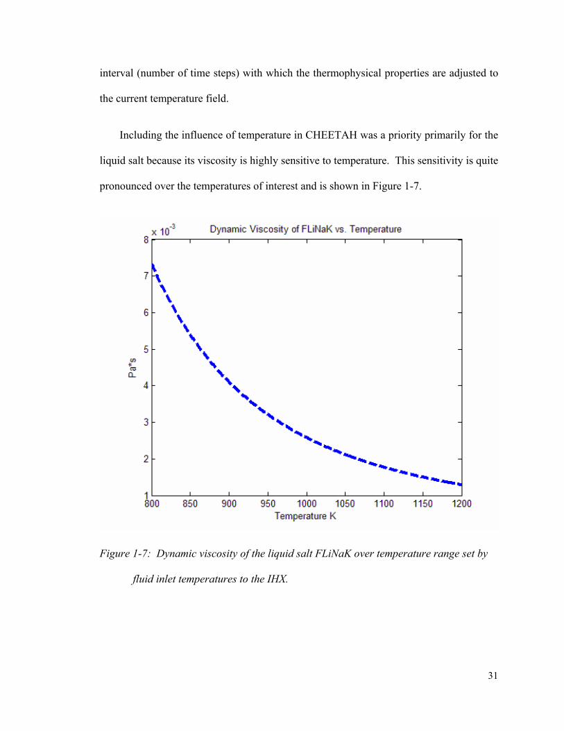
31
interval (number of time steps) with which the thermophysical properties are adjusted to
the current temperature field.
Including the influence of temperature in CHEETAH was a priority primarily for the
liquid salt because its viscosity is highly sensitive to temperature. This sensitivity is quite
pronounced over the temperatures of interest and is shown in Figure 1-7.
Figure 1-7: Dynamic viscosity of the liquid salt FLiNaK over temperature range set by
fluid inlet temperatures to the IHX.
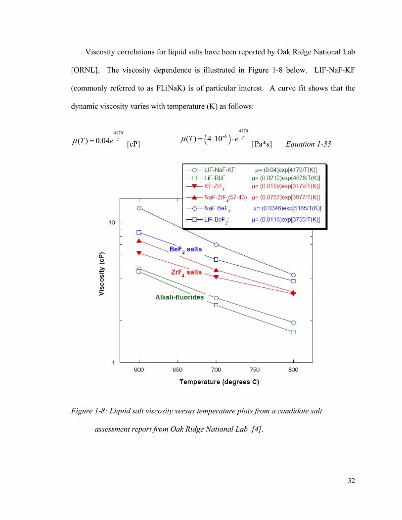
32
Viscosity correlations for liquid salts have been reported by Oak Ridge National Lab
[ORNL]. The viscosity dependence is illustrated in Figure 1-8 below. LIF-NaF-KF
(commonly referred to as FLiNaK) is of particular interest. A curve fit shows that the
dynamic viscosity varies with temperature (K) as follows:
4170
( ) 0.04 TT eμ = [cP] ( )4170
5( ) 4 10 TT eμ −= ⋅ ⋅ [Pa*s] Equation 1-33
Figure 1-8: Liquid salt viscosity versus temperature plots from a candidate salt
assessment report from Oak Ridge National Lab [4].

33
The temperature dependency of viscosity, specific heat, and density are graphed for
helium at 7 MPa using values obtained from a NIST web book [16] in Figure 1-9 below.
From these charts it is clear that the variation in specific heat is insignificant (.01%)
compared with those for viscosity and density over the heat exchanger’s temperature
range. The viscosity of helium increases nearly linearly with temperature in this range
and density varies inversely with temperature as dictated by the ideal gas law. The
helium density can be found by applying the ideal gas law with an error less than 1%,
when compared to the values tabulated in NIST. The table of thermophysical properties
for high pressure helium is available in Appendix B.

34
Figure 1-9: Isobaric thermophysical properties for helium at 7MPa from NIST.
35
Chapter 2
Partitioning, Discretization,
and Numerical Method
In modeling the IHX, the actual material properties can be set and changed with great
ease, as they are simply represented by a series of constants assigned in the input file
(Systems Properties module) of the CHEETAH code. However, the fluidic, thermal, and
mechanical response of the solid media comes from geometric effects that are central to
the model’s validity. This is where the EPM model simplifies the problem by creating
mass and energy balances at a scale that will both include the complexity of the thermal
hydraulics in the IHX and also yield results in a reasonable time period to permit fluidic,
thermal, and mechanical improvements to the IHX design over various iterations.
Calculating the effective conductivities, permeabilities, phase fractions, surface area
densities, convection coefficients, effective elastic moduli, shear moduli, and Poisson’s
ratios is very labor intensive because it takes over 20 unique zones with different media
properties to fully describe the hydraulic, thermal, and mechanical properties of a typical
compact heat exchanger. Some of these properties are calculated with correlations within
the CHEETAH code, but others must be calculated on separate software (such as FEA
and design software) and added to the input files. The nodal assignment of the above

36
mentioned properties onto the array representing the IHX geometry is entirely automated
and executed with various scripts within the CHEETAH code.
2.1 Zoning the IHX
The pressure and velocity distributions in the IHX are solved for both fluid phases by
breaking up the IHX into over 20 flow zones. Each of these zones has unique physical
properties that govern the flow for each of the two phases. Figure 2-1 shows the zoning
for the composite plate.
For the case of an IHX that transfers heat between a liquid and a gas, it is
representative to take the case of liquid salt for the liquid and helium as the gas. This is
particularly relevant as they are among the fluid choices being considered by the U.S.
Department of Energy’s Next Generation Nuclear Plant (NGNP).
The heat transfer analysis has been developed progressively starting with one-
dimensional models that neglected longitudinal (main flow direction, x) conduction to
two-dimensional models that include cross-flow in the fluids as well as spatially varying
longitudinal and latitudinal (cross-flow direction, z) conduction. Early models used
constant convection coefficients and surface area densities; the current analysis includes
the spatial variation of all thermal and hydraulic parameters including temperature-
dependent fluid properties.
37
The assignment of the geometry-dependent property distributions is a complex and
essential function within the EPM model implemented in the CHEETAH code. The
central purpose of the CHEETAH code is to enable the designer to simulate the
performance of the IHX for a given geometry and set of dimensions; the heat exchanger
design can then be improved in an iterative fashion based on the results of the simulation.
Changing the dimensions of the IHX, fins, channels, and size of distributor channels in
CHEETAH is accomplished by changing values in the input parameters file; however,
significant changes to the shape of the IHX or manifolds require coding.
The CHEETAH code contains a long set of system parameters that define the external
and internal geometry. The code will automatically change the zone boundaries so that
the user does not have to modify the code with every dimensional variation. Manual
modification of the code may be necessary if any of the dimensions approach the grid
size or if the shape of the IHX is modified. A schematic drawing of the IHX’s composite
plate, Figure 2-1, shows the layout of zones where different thermal hydraulic parameters
are defined. These zones apply the spatially varying phase fractions, surface area
densities, convection coefficients, directional permeability, and directional effective
conductivities in the IHX.
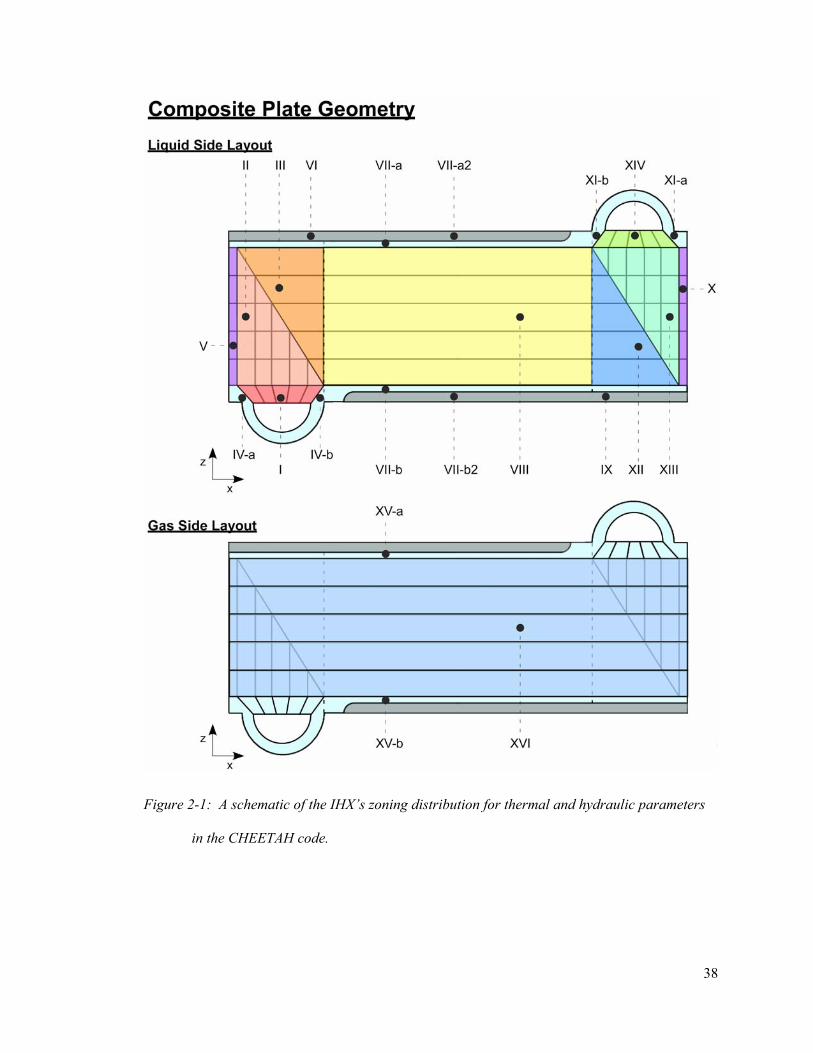
38
Figure 2-1: A schematic of the IHX’s zoning distribution for thermal and hydraulic parameters
in the CHEETAH code.
39
Zones IV-a, IV-b, VII-a, VII-b, XI-a, XI-b, XV-a, and XV-b, shown in light turquoise
in Figure 2-1, represent a structural area where no fluid flows. For this reason, the areas
have a phase fraction of 100% (φ=1), no surface density, and no convection coefficient.
These zones will have a greater thermal inertia and will in general take longer to
equilibrate during thermal transients. These zones will also have higher effective
conductivity in all directions because the entire cross-section is available for heat flow,
which reduces thermal resistance.
2.2 Diffuser and Reducer Permeability
The schematic drawing above is also simplified in the diffuser (zone I) and reducer
(zone XIV) areas, which are shown as trapezoids. In these zones, every control volume
has unique effective properties assigned to it depending on the local channel geometry
being represented by the EPM. In order to accurately represent the local geometry, the
assigned EPM uses the angle and spacing of the channels nearest to the node in the actual
IHX. The CHEETAH code accomplishes this by finding the position of each node and
the slope of the line connecting the node point to a central fictitious point to which the
flow distribution channels align. Using the point and slope information for each node
and the line equation from adjacent channels, the CHEETAH code finds the normal
distance between channels at that node point and uses this to calculate a multiplier for the
directional permeability so that the effective flow and cross-flow permeabilities at that
node take into consideration not only the alignment of the channel but also the local
40
channel density. These zones are shown in a uniform color here for simplicity, but each
also includes other parameters that allow the CHEETAH code user to manipulate the
flow distribution. This will be discussed further in the next section. Schematic drawings
similar to Figure 2-1 would illustrate the layout of other effective property values such as
effective conductivities, permeabilities, porosities, surface area densities, convection
coefficients, effective elastic moduli, shear moduli, and Poisson’s ratios for the IHX.
2.3 Adjustable Flow Distribution
Improving the thermal design of a heat exchanger involves designing the device in
such a way as to increase its thermal effectiveness. The thermal effectiveness is a ratio of
heat actually exchanged between the hot and cold fluids to the maximum amount of heat
that can be transferred between them given fluid inlet temperatures, specific heats, and
flow rates. More generally, it is a number between zero and one that quantifies the
performance of a thermal device. More detailed explanation on thermal effectiveness is
available in texts by Mills [17], Incropera [18], and Çengel [19].
To increase the thermal effectiveness, it is crucial to create and maintain uniform flow
in the heat exchanger in order to utilize the heat transfer surface area as uniformly as
possible. Uniform flow increases the average residency of the fluid in the heat
exchanger, which in turn increases total heat transfer. This is more obvious when
considering that the convection coefficient is proportional to the square root of the
Reynolds number. Therefore, flow maldistribution will create areas with higher flow

41
speeds and therefore with higher heat transfer rates, but this comes at the more significant
detriment of flow in other areas and therefore at the detriment of total heat transfer.
In order to create and maintain uniform flow though the IHX, the CHEETAH code
accommodates the channel orientation and channel density in the nodal permeability
assignment of the liquid plate. The distributors are in the liquid salt plate because that is
where flow maldistribution is most likely to occur since the liquid salt viscosity is
significantly more temperature-dependent [4]. The code also allows the designer to
manually tune a multiplier coefficient for distinct zones in the sections containing the
flow distribution channels. The adjustable permeability in these zones allows the user to
quickly and directly manipulate the flow distribution as if controlling independent and
parallel valves leading into and out of the OSF section. Shown in varying shades of
yellow, the distributor channels in the liquid inlet can be seen in the liquid plate
schematic drawing in Figure 2-2. The flow distributors for the liquid outlet can be seen
in varying shades of green in Figure 2-2.
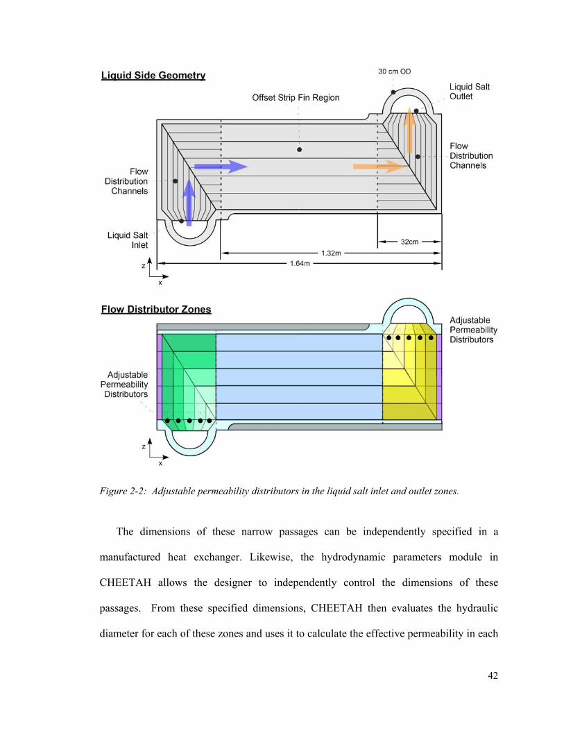
42
Figure 2-2: Adjustable permeability distributors in the liquid salt inlet and outlet zones.
The dimensions of these narrow passages can be independently specified in a
manufactured heat exchanger. Likewise, the hydrodynamic parameters module in
CHEETAH allows the designer to independently control the dimensions of these
passages. From these specified dimensions, CHEETAH then evaluates the hydraulic
diameter for each of these zones and uses it to calculate the effective permeability in each
43
zone. The zones representing the distribution channels in the EPM model can be seen in
Figure 2-1. These features in CHEETAH enable the control the flow distribution in the
offset strip fin region where most of heat transfer takes place. In this region a small
maldistribution of flow can significantly influence total heat exchanger effectiveness.
The lower flow resistance associated with the shortest flow path in the inlet manifold
is already balanced by a higher flow resistance created by the corresponding longer flow
path in the outlet manifold, so that the total flow resistance is roughly equal regardless of
the path followed. However, there are still issues with flow maldistribution in the IHX.
Among the factors that affect the flow distribution are the temperature-dependent
viscosity effects (discussed in the next chapter) and the fact that the paths nearest the
inner corners of each region are shortest and therefore have higher flow rates than the
outside corners in each flow region.
Each inlet region is separated into several flow regions representing the flow
distribution channels. The number of flow regions is specified by the assignment of a
constant in CHEETAH’s System Parameters module. The manifolds can be divided into
any number of flow regions, but it is important to maintain a region width of at least three
cells across to avoid discretization errors such as stair-casing, where the coarse mesh
creates abrupt reductions in flow area and therefore peak velocities that can lead to
instabilities by way of excessive CFL (Courant – Friedrichs – Levy = u*Δt/Δx) numbers.
44
2.4 Specifying the Grid
The CHEETAH code is written in Matlab and uses a rectangular mesh which fits the
rectangular geometry of the IHX. The code was originally written with a typical
rectangular grid, such that each node point lay in the center of the control surface and was
identified by four coordinates (x-position, y-position, z-position, iteration number) with
the following indexes (i,j,k,n), as is shown in Figure 2-3. The y-position (j index) in the
rectangular grid connotes the phase with index 1 and index 3 being the fluids and index 2
always representing the solid phase. The CHEETAH Code was later improved by
replacing the simple rectangular grid with a more sophisticated staggered grid.
The x and z-position coordinates (indices) associated with every node provide a
physical Cartesian dimension for the node’s location on the IHX geometry (with respect
to an origin) when they are multiplied by the corresponding spatial discretization (Δx and
Δz, respectively). Those Cartesian dimensions place the node within one of the
previously delineated zones which in turn leads to the assignment of the corresponding
local physical properties such as effective conductivities, permeabilities, porosities,
surface area densities, convection coefficients, effective elastic moduli, shear moduli, and
Poisson’s ratios according to the zoning described previously.
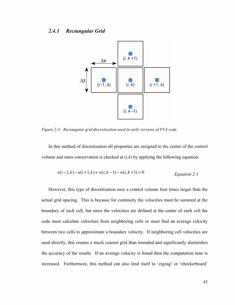
45
2.4.1 Rectangular Grid
Figure 2-3: Rectangular grid discretization used in early versions of FVA code.
In this method of discretization all properties are assigned to the center of the control
volume and mass conservation is checked at (i,k) by applying the following equation:
( 1, ) ( 1, ) ( , 1) ( , 1) 0u i k u i k w i k w i k− − + + − − + = Equation 2-1
However, this type of discretization uses a control volume four times larger than the
actual grid spacing. This is because for continuity the velocities must be summed at the
boundary of each cell, but since the velocities are defined at the center of each cell the
code must calculate velocities from neighboring cells or must find an average velocity
between two cells to approximate a boundary velocity. If neighboring cell velocities are
used directly, this creates a much coarser grid than intended and significantly diminishes
the accuracy of the results. If an average velocity is found then the computation time is
increased. Furthermore, this method can also lend itself to ‘zigzag’ or ‘checkerboard’
46
pressure or temperature distributions since the continuity and momentum equations use
information from alternating nodes to check for continuity [20]. Essentially, this means
that a wavy pressure distribution will produce a wavy velocity distribution that can
satisfy continuity, since it is information from alternating and not adjacent nodes that
must satisfy continuity [20].
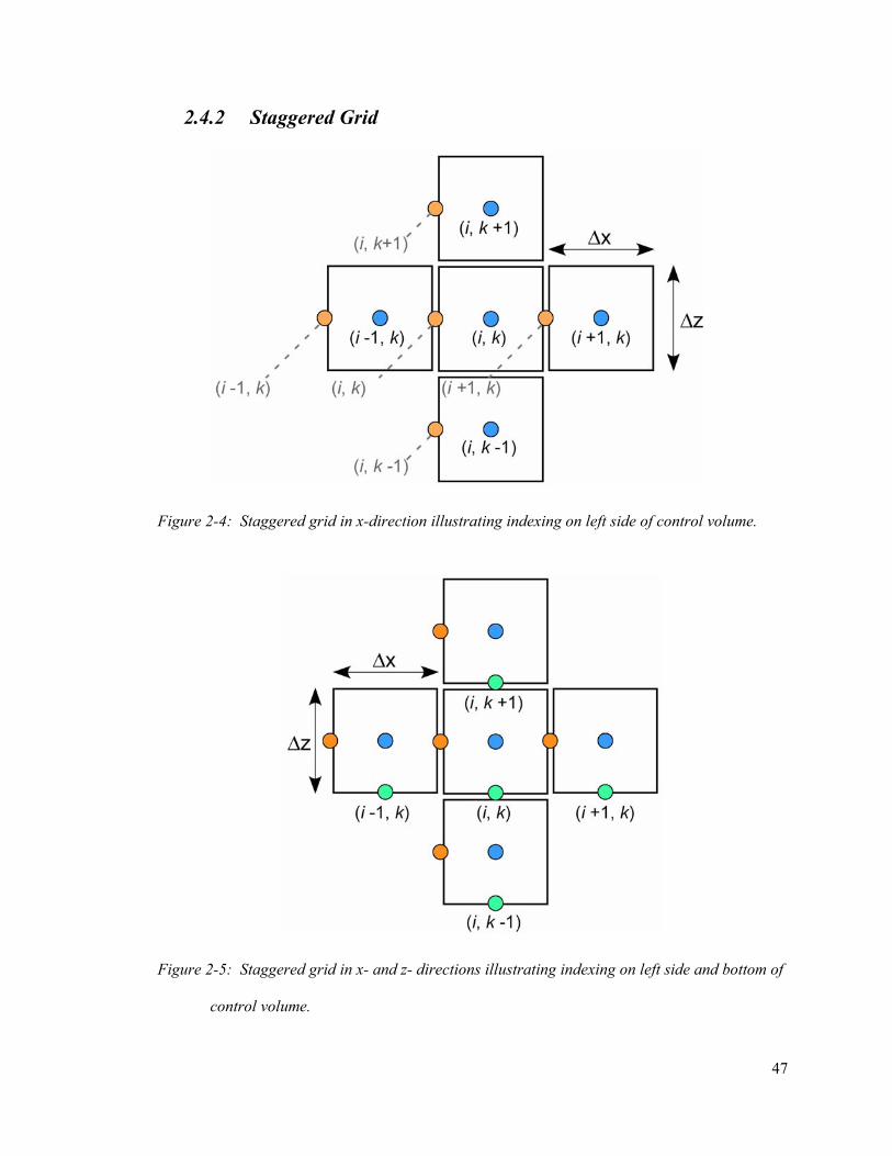
47
2.4.2 Staggered Grid
Figure 2-4: Staggered grid in x-direction illustrating indexing on left side of control volume.
Figure 2-5: Staggered grid in x- and z- directions illustrating indexing on left side and bottom of
control volume.
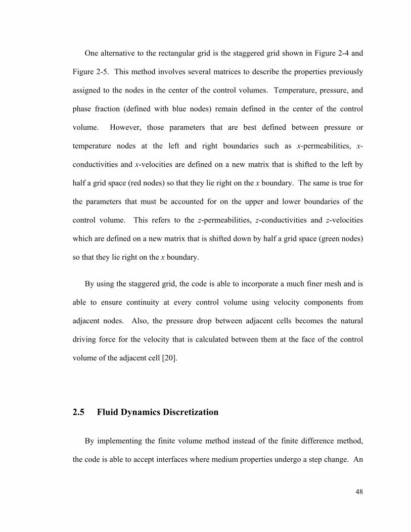
48
One alternative to the rectangular grid is the staggered grid shown in Figure 2-4 and
Figure 2-5. This method involves several matrices to describe the properties previously
assigned to the nodes in the center of the control volumes. Temperature, pressure, and
phase fraction (defined with blue nodes) remain defined in the center of the control
volume. However, those parameters that are best defined between pressure or
temperature nodes at the left and right boundaries such as x-permeabilities, x-
conductivities and x-velocities are defined on a new matrix that is shifted to the left by
half a grid space (red nodes) so that they lie right on the x boundary. The same is true for
the parameters that must be accounted for on the upper and lower boundaries of the
control volume. This refers to the z-permeabilities, z-conductivities and z-velocities
which are defined on a new matrix that is shifted down by half a grid space (green nodes)
so that they lie right on the x boundary.
By using the staggered grid, the code is able to incorporate a much finer mesh and is
able to ensure continuity at every control volume using velocity components from
adjacent nodes. Also, the pressure drop between adjacent cells becomes the natural
driving force for the velocity that is calculated between them at the face of the control
volume of the adjacent cell [20].
2.5 Fluid Dynamics Discretization
By implementing the finite volume method instead of the finite difference method,
the code is able to accept interfaces where medium properties undergo a step change. An
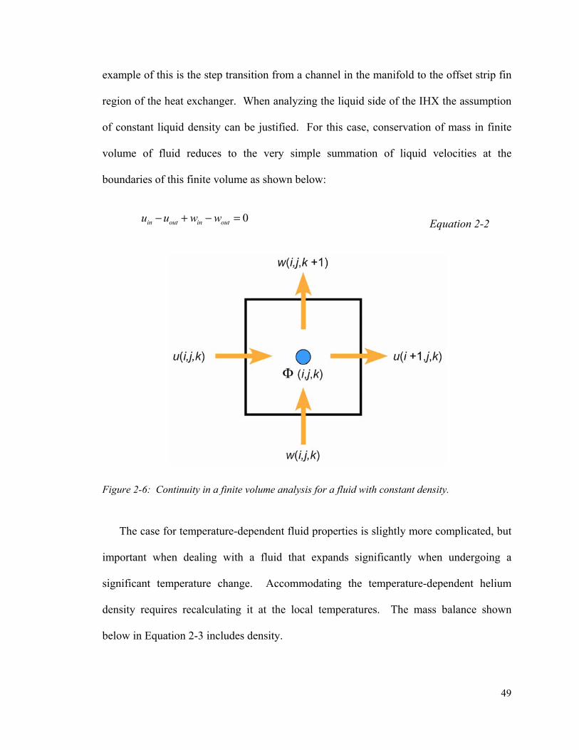
49
example of this is the step transition from a channel in the manifold to the offset strip fin
region of the heat exchanger. When analyzing the liquid side of the IHX the assumption
of constant liquid density can be justified. For this case, conservation of mass in finite
volume of fluid reduces to the very simple summation of liquid velocities at the
boundaries of this finite volume as shown below:
0in out in outu u w w− + − = Equation 2-2
Figure 2-6: Continuity in a finite volume analysis for a fluid with constant density.
The case for temperature-dependent fluid properties is slightly more complicated, but
important when dealing with a fluid that expands significantly when undergoing a
significant temperature change. Accommodating the temperature-dependent helium
density requires recalculating it at the local temperatures. The mass balance shown
below in Equation 2-3 includes density.

50
1, , , , , , 1, , , , 1 , , , , , , 1 0i j k i j k i j k i j k i j k i j k i j k i j ku u w wρ ρ ρ ρ− + − +− + − = Equation 2-3
While the mass balance above depicts velocity, in CHEETAH the velocity is replaced
by a discretized form of Darcy’s transport equation such that the velocity terms actually
introduce temperature-dependent viscosity, location-specific permeability and
surrounding pressures as shown below in Equation 2-4:
, , _ , , , , 1, , 1, , _ 1, , 1, , , ,
, , 1, ,
...i j k x i j k i j k i j k i j k x i j k i j k i j k
i j k i j k
k kx x
ρ ρμ μ
− + + +
+
Φ − Φ Φ − Φ⎛ ⎞ ⎛ ⎞− +⎜ ⎟ ⎜ ⎟Δ Δ⎝ ⎠ ⎝ ⎠
, , _ , , , , , , 1 , , 1 _ , , 1 , , 1 , ,
, , , , 1
0i j k z i j k i j k i j k i j k z i j k i j k i j k
i j k i j k
k kz z
ρ ρμ μ
− + + +
+
Φ − Φ Φ − Φ⎛ ⎞ ⎛ ⎞− + =⎜ ⎟ ⎜ ⎟Δ Δ⎝ ⎠ ⎝ ⎠
Equation 2-4
Incorporating this into the discretization is complicated slightly by deciding which
density values to use with each velocity. This is important both in the mass and energy
balance in order to maintain stability. Unlike velocity, which is defined at the volume
boundary, density is defined by the temperature of the cell which is in turn defined at the
center or node. It is important that the mass entering the cell have the density of the cell
from which it is departing. This is seemingly simple, but when fluid can be moving in
any direction the code must be able to adapt and use the appropriate density depending on
the sign of the velocity. The correct values have been assigned below in Figure 2-7.
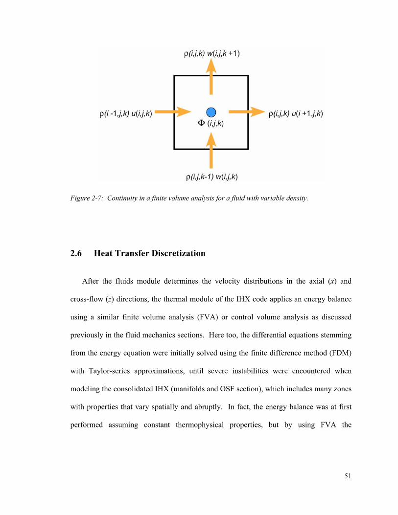
51
Figure 2-7: Continuity in a finite volume analysis for a fluid with variable density.
2.6 Heat Transfer Discretization
After the fluids module determines the velocity distributions in the axial (x) and
cross-flow (z) directions, the thermal module of the IHX code applies an energy balance
using a similar finite volume analysis (FVA) or control volume analysis as discussed
previously in the fluid mechanics sections. Here too, the differential equations stemming
from the energy equation were initially solved using the finite difference method (FDM)
with Taylor-series approximations, until severe instabilities were encountered when
modeling the consolidated IHX (manifolds and OSF section), which includes many zones
with properties that vary spatially and abruptly. In fact, the energy balance was at first
performed assuming constant thermophysical properties, but by using FVA the

52
thermophysical properties are free to vary with local temperature and pressure, and the
result is still highly stable.
The energy balances on a finite volume in each phase are presented below (Figure
2-8, Figure 2-9, and Figure 2-10) using pressure and temperature-dependent density for
the gas.
2.6.1 Control Volume for Liquid Phase in the IHX
Figure 2-8: Energy balance in the finite volume analysis for a fluid with constant density.
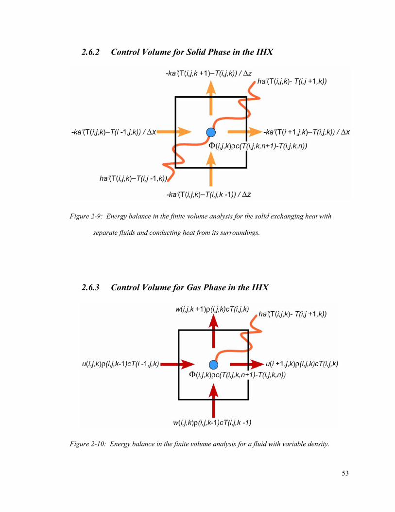
53
2.6.2 Control Volume for Solid Phase in the IHX
Figure 2-9: Energy balance in the finite volume analysis for the solid exchanging heat with
separate fluids and conducting heat from its surroundings.
2.6.3 Control Volume for Gas Phase in the IHX
Figure 2-10: Energy balance in the finite volume analysis for a fluid with variable density.

54
Chapter 3
Thermal Hydraulic Results
This chapter presents thermal hydraulic results from analyses from the Compact Heat
Exchanger Thermal and Hydraulic (CHEETAH) code using both constant and
temperature-dependent thermophysical properties. The analysis includes steady-state
plots of pressure, velocity, and temperature for both constant and temperature-dependent
thermophysical properties for comparison. Transient thermal hydraulic results are also
presented for the case of constant thermophysical properties.
3.1 CHEETAH Code Architecture
The CHEETAH code consists of five modules. Each module executes code that
either assigns system characteristics, thermal hydraulics parameters, or performs the
finite volume analyses presented in the previous chapter. The modules are described in
Figure 3-1 below.
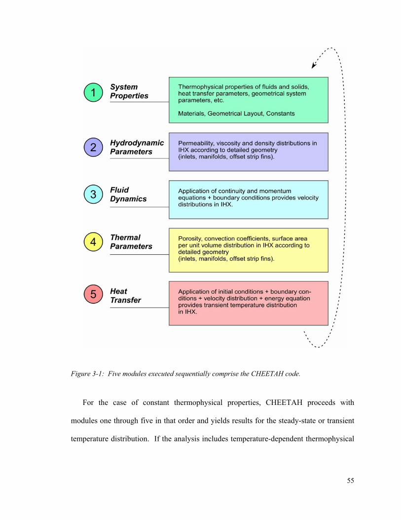
55
Figure 3-1: Five modules executed sequentially comprise the CHEETAH code.
For the case of constant thermophysical properties, CHEETAH proceeds with
modules one through five in that order and yields results for the steady-state or transient
temperature distribution. If the analysis includes temperature-dependent thermophysical

56
fluid properties, then the steady-state temperature distribution is obtained by running
modules one through five and the resulting temperature distribution used to find
distributions in the thermophysical properties. Subsequently pressure and velocity
distributions are again calculated by executing modules two through five with new
thermophysical properties. In theory, the best solution would be obtained by
implementing modules two through five at every time step in module five, since that
would apply the most recent temperature data to the thermophysical properties, but the
computational time would be exorbitant. The frequency with which thermophysical
properties and fluid dynamics are updated is set by the user. In the analysis for
temperature-dependent thermophysical properties presented later, the steady-state
distribution is used to set thermophysical properties and fluid dynamics.
3.2 Thermal Hydraulic Results with Constant Thermophysical Properties
The thermal hydraulic results from CHEETAH using constant thermophysical
properties are presented because they help benchmark the effect and importance of
including temperature-dependent thermophysical properties in the finite volume analysis
(FVA) used in CHEETAH. For the following results the viscosity of both fluids is
evaluated at each fluid’s median temperature (half-way through the OSF region) through
the IHX. The change in density of the liquid salt is not significantly affected by
temperature and thus will be treated as constant in this analysis. The density of helium
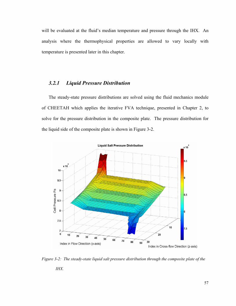
57
will be evaluated at the fluid’s median temperature and pressure through the IHX. An
analysis where the thermophysical properties are allowed to vary locally with
temperature is presented later in this chapter.
3.2.1 Liquid Pressure Distribution
The steady-state pressure distributions are solved using the fluid mechanics module
of CHEETAH which applies the iterative FVA technique, presented in Chapter 2, to
solve for the pressure distribution in the composite plate. The pressure distribution for
the liquid side of the composite plate is shown in Figure 3-2.
Figure 3-2: The steady-state liquid salt pressure distribution through the composite plate of the
IHX.
58
The shape of the pressure gradient over the IHX clearly denotes areas with different
permeabilities and delineates the interfaces where the permeability changes. Changes in
the pressure gradient can be seen where the OSF sections meet the inlet and outlet
manifold producing an edge in the distribution. This identifies the interface without the
instabilities created when analyzed with the Taylor-series based finite difference
techniques. The zones nearest the inlet and outlet ports in Figure 3-2 show that most of
hydraulic head is depleted in the distribution channels between the inlet port and the
offset strip fin (OSF) region. This configuration is specified because the higher flow
resistance in the flow distributor channels allows the determination of the flow going into
each zone within the OSF section and which may be altered by changing the flow
resistance in the distribution channels leading to and following any zone in the OSF
section. The index on the x and z axis represent the number of finite volumes with each
index locating a finite volume cube that measures 2 cm on each side.
3.2.2 Gas Pressure Distribution
The pressure distribution in the gas side of the composite plate is readily obtained
when using constant thermophysical properties. The permeabilities in both the flow and
cross-flow directions through the center of the gas side of the composite plate are
constant. The constant permeabilities in this region result in a linear helium pressure
distribution through the plate. The helium pressure distribution for constant density and
viscosity is shown in Figure 3-3.

59
Figure 3-3: The steady-state helium pressure distribution through the composite plate of the
IHX.
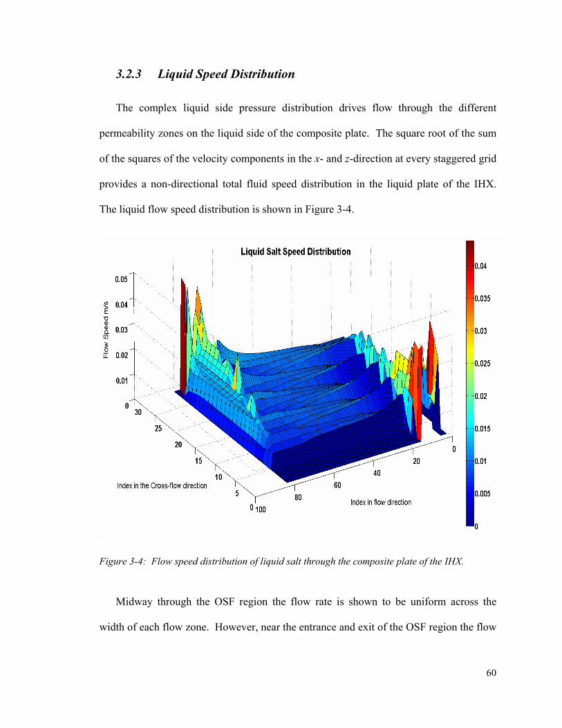
60
3.2.3 Liquid Speed Distribution
The complex liquid side pressure distribution drives flow through the different
permeability zones on the liquid side of the composite plate. The square root of the sum
of the squares of the velocity components in the x- and z-direction at every staggered grid
provides a non-directional total fluid speed distribution in the liquid plate of the IHX.
The liquid flow speed distribution is shown in Figure 3-4.
Figure 3-4: Flow speed distribution of liquid salt through the composite plate of the IHX.
Midway through the OSF region the flow rate is shown to be uniform across the
width of each flow zone. However, near the entrance and exit of the OSF region the flow
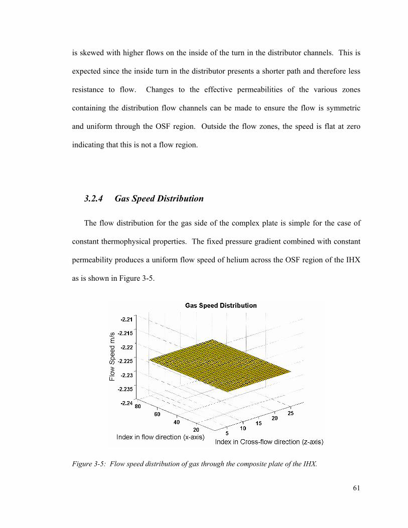
61
is skewed with higher flows on the inside of the turn in the distributor channels. This is
expected since the inside turn in the distributor presents a shorter path and therefore less
resistance to flow. Changes to the effective permeabilities of the various zones
containing the distribution flow channels can be made to ensure the flow is symmetric
and uniform through the OSF region. Outside the flow zones, the speed is flat at zero
indicating that this is not a flow region.
3.2.4 Gas Speed Distribution
The flow distribution for the gas side of the complex plate is simple for the case of
constant thermophysical properties. The fixed pressure gradient combined with constant
permeability produces a uniform flow speed of helium across the OSF region of the IHX
as is shown in Figure 3-5.
Figure 3-5: Flow speed distribution of gas through the composite plate of the IHX.
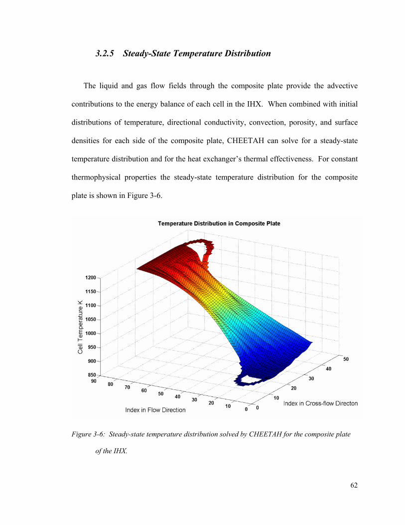
62
3.2.5 Steady-State Temperature Distribution
The liquid and gas flow fields through the composite plate provide the advective
contributions to the energy balance of each cell in the IHX. When combined with initial
distributions of temperature, directional conductivity, convection, porosity, and surface
densities for each side of the composite plate, CHEETAH can solve for a steady-state
temperature distribution and for the heat exchanger’s thermal effectiveness. For constant
thermophysical properties the steady-state temperature distribution for the composite
plate is shown in Figure 3-6.
Figure 3-6: Steady-state temperature distribution solved by CHEETAH for the composite plate
of the IHX.
63
Ridges in the temperature distribution can be seen in the OSF region of the IHX.
These edges make the flow zone easy to identify in the OSF region. The sharp gradients
in the temperature distribution are formed by discrepancies between the flow rates and
flow paths in neighboring flow zones in the IHX. These are the same ridges that were
discussed in Figure 3-4 showing the speed distribution; they help to demonstate the
impact of minor variations in flow on heat exchanger performance.
64
3.2.6 Transient Temperature Distributions
Two thermal transients are considered in this analysis. One analyzes the transient
temperature distributions that result from the interruption of liquid flow while the other
concerns the interruption of gas flow to the IHX. In both cases the flow is
instantaneously reduced to 2% of the steady-state mass flow rate. This reduced-flow
value is arbitrary and is meant to put the IHX into a severe thermal transient. The
simulation would be more representative of an operational scenario if it included a
gradual pump coast down resulting in a ramped reduction of flow rather than a stepped
reduction. The CHEETAH code is capable of executing any flow ramp down but doing
so would require empirical pump coast-down data from a specific pump. A more severe
transient results with a step change in flow.
The transient is assumed to begin from a steady-state operation condition and the
temperature distribution of the composite plate of the IHX is examined. In both cases, a
similar transient could occur from a severe pump or valve failure in a power plant. The
transient analyses presented here were analyzed using CHEETAH using constant
thermophysical properties where the IHX is assumed to be in a horizontal arrangement.
If the IHX were to be modeled in a vertical arrangement the more complicated effects of
natural circulation would need to be modeled as well. In each case it is assumed that one
fluid experiences a step change in flow while the counter-flowing fluid continues to flow
unhindered. This further increases the severity of the thermal transient on the resulting
mechanical stresses. The CHEETAH code solves for the temperature profiles in the
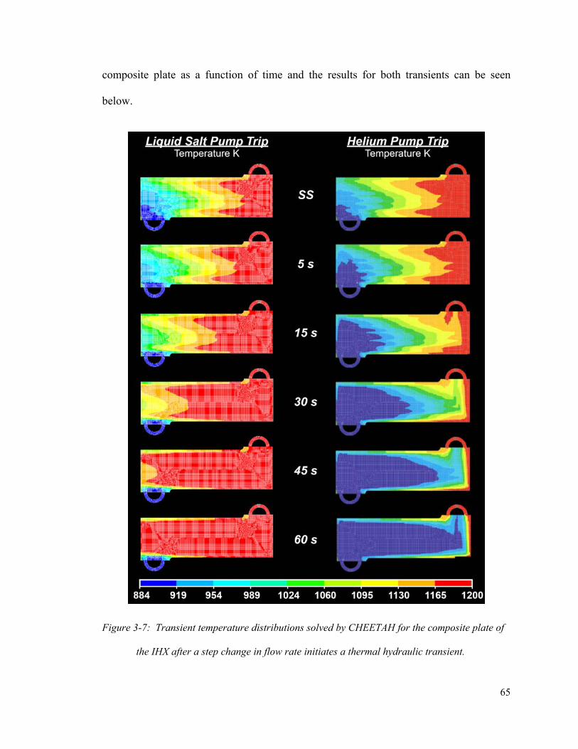
65
composite plate as a function of time and the results for both transients can be seen
below.
Figure 3-7: Transient temperature distributions solved by CHEETAH for the composite plate of
the IHX after a step change in flow rate initiates a thermal hydraulic transient.
66
The thermal hydraulic transient begins from a steady-state temperature distribution in
both cases. The steady-state temperature distribution is marked SS in Figure 3-7. The
contours marking the temperature gradients show a lack of symmetry in the temperature
distribution, which are shown clearly near the liquid salt (cold fluid) inlet on the bottom
left of the heat exchanger in the plot marked SS. In the steady-state plots the temperature
profiles follow the cold fluid (liquid salt) flow directions in the colder left-hand side of
the IHX. The hotter (right-hand) side of the composite plate is clearly dominated by the
ingress of hot helium to the point that temperature gradients are not visible near the liquid
salt outlet port which is within 35 K of the inlet temperature.
In the liquid salt pump trip transient the colder liquid salt is instantaneously reduced
to 2% of its original flow rate while the hotter helium flow continues. The five second
graph (5 s) shows all temperature profiles for the liquid salt pump trip advance leftward;
after 30 seconds (30 s) from the initiating liquid salt pump trip the shape of these
temperature fronts change slightly as they encounter regions of the composite plate with
varying temperatures. After roughly 60 seconds (60 s) the new steady-state profile is
generally in place. The small cold region near the liquid salt inlet will remain within 35
K of the liquid salt inlet temperature due to the residual post-transient flow (2% of initial
flow rate) entering the composite plate. The phenomena associated with this residual
flow could be representative of buoyancy effects in other parts of the intermediate loop or
in a vertically-oriented IHX.
The progression of the temperature fronts along the more complicated liquid salt flow
paths in the composite plate is clear in the helium pump trip transient shown on the left
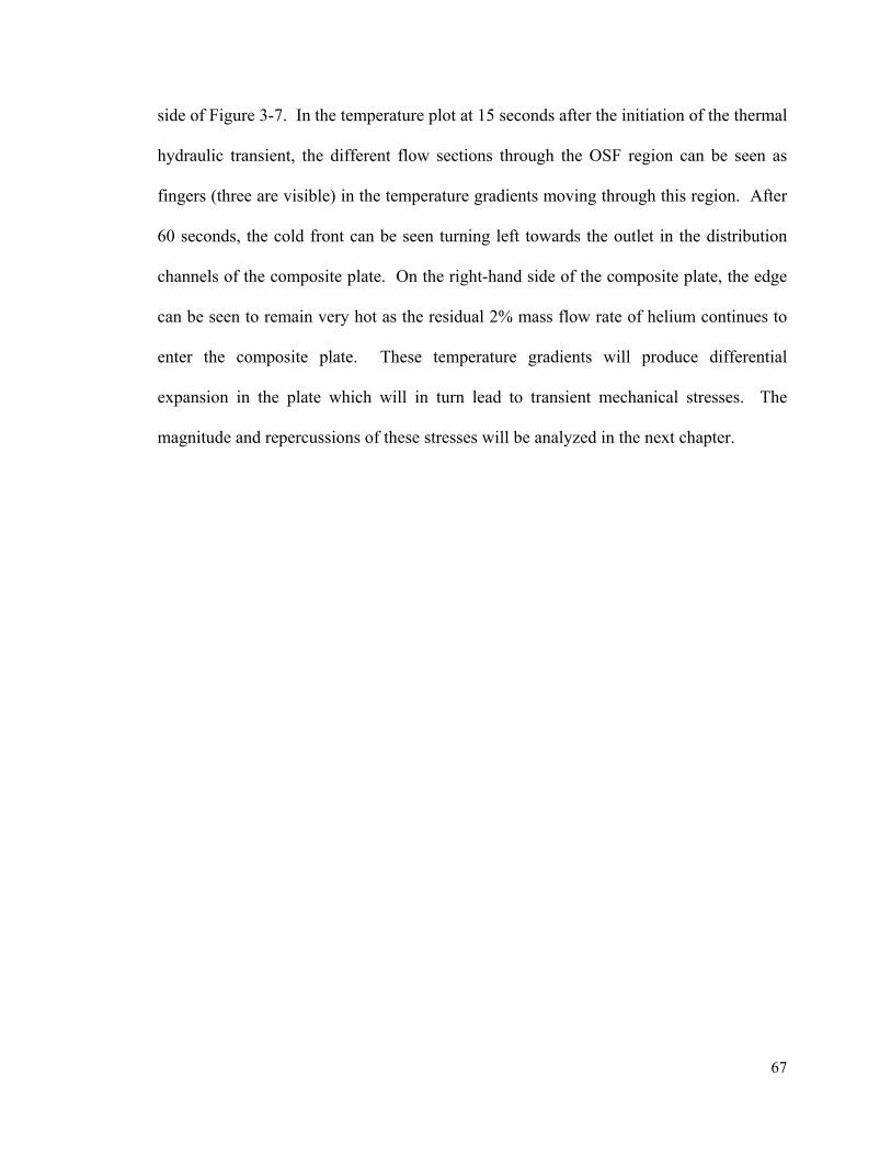
67
side of Figure 3-7. In the temperature plot at 15 seconds after the initiation of the thermal
hydraulic transient, the different flow sections through the OSF region can be seen as
fingers (three are visible) in the temperature gradients moving through this region. After
60 seconds, the cold front can be seen turning left towards the outlet in the distribution
channels of the composite plate. On the right-hand side of the composite plate, the edge
can be seen to remain very hot as the residual 2% mass flow rate of helium continues to
enter the composite plate. These temperature gradients will produce differential
expansion in the plate which will in turn lead to transient mechanical stresses. The
magnitude and repercussions of these stresses will be analyzed in the next chapter.
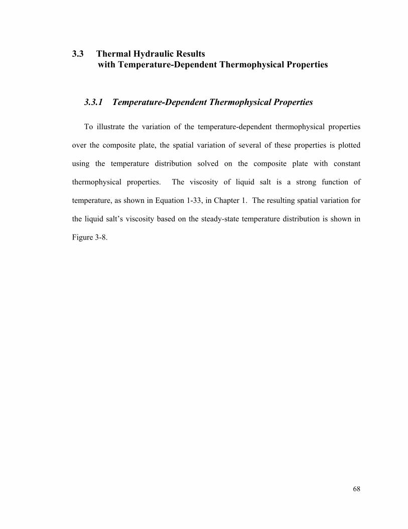
68
3.3 Thermal Hydraulic Results with Temperature-Dependent Thermophysical Properties
3.3.1 Temperature-Dependent Thermophysical Properties
To illustrate the variation of the temperature-dependent thermophysical properties
over the composite plate, the spatial variation of several of these properties is plotted
using the temperature distribution solved on the composite plate with constant
thermophysical properties. The viscosity of liquid salt is a strong function of
temperature, as shown in Equation 1-33, in Chapter 1. The resulting spatial variation for
the liquid salt’s viscosity based on the steady-state temperature distribution is shown in
Figure 3-8.
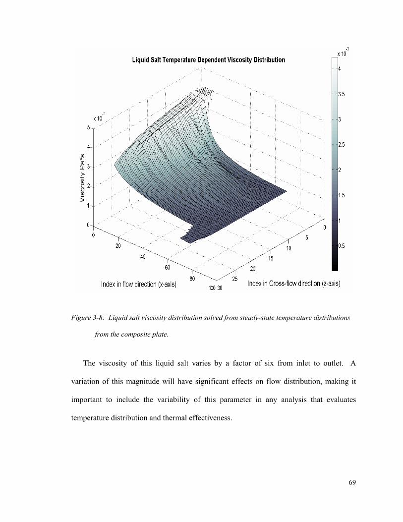
69
Figure 3-8: Liquid salt viscosity distribution solved from steady-state temperature distributions
from the composite plate.
The viscosity of this liquid salt varies by a factor of six from inlet to outlet. A
variation of this magnitude will have significant effects on flow distribution, making it
important to include the variability of this parameter in any analysis that evaluates
temperature distribution and thermal effectiveness.
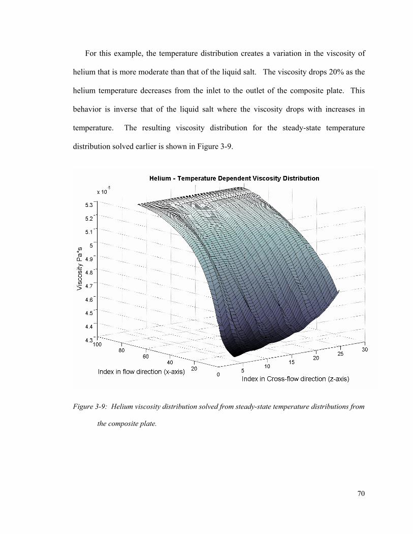
70
For this example, the temperature distribution creates a variation in the viscosity of
helium that is more moderate than that of the liquid salt. The viscosity drops 20% as the
helium temperature decreases from the inlet to the outlet of the composite plate. This
behavior is inverse that of the liquid salt where the viscosity drops with increases in
temperature. The resulting viscosity distribution for the steady-state temperature
distribution solved earlier is shown in Figure 3-9.
Figure 3-9: Helium viscosity distribution solved from steady-state temperature distributions from
the composite plate.
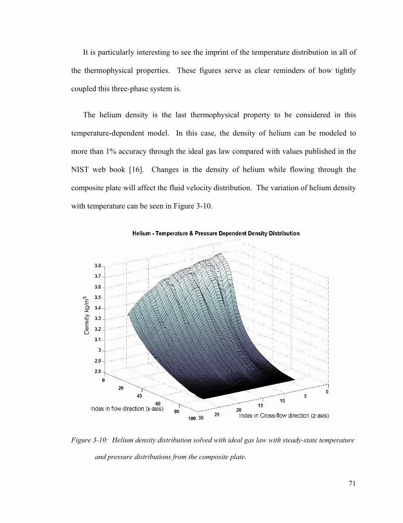
71
It is particularly interesting to see the imprint of the temperature distribution in all of
the thermophysical properties. These figures serve as clear reminders of how tightly
coupled this three-phase system is.
The helium density is the last thermophysical property to be considered in this
temperature-dependent model. In this case, the density of helium can be modeled to
more than 1% accuracy through the ideal gas law compared with values published in the
NIST web book [16]. Changes in the density of helium while flowing through the
composite plate will affect the fluid velocity distribution. The variation of helium density
with temperature can be seen in Figure 3-10.
Figure 3-10: Helium density distribution solved with ideal gas law with steady-state temperature
and pressure distributions from the composite plate.

72
3.3.2 Liquid Pressure Distribution
The steady-state pressure distributions are solved by the fluid mechanics module of
CHEETAH considering liquid salt’s viscosity variation with temperature. The code can
be set to recalculate the viscosity distribution based on the current temperature
distribution as often as necessary. The more often the thermophysical properties are
updated with the temperature distribution, the more accurate the flow distribution will be,
but the longer the code will take to find the steady-state flow distribution. The pressure
distribution for the liquid side of the composite plate is based on temperature-dependent
thermophysical properties, which are in turn based on the temperature distribution found
in the previous section. The resulting pressure distributions are shown in Figure 3-11.

73
Figure 3-11: The steady-state liquid salt pressure distribution through the composite plate of the
IHX with temperature-dependent thermophysical properties.
The liquid salt inlet can be found in Figure 3-11 because it has the highest pressure
and is shown in red near coordinates (0,0). The liquid salt outlet manifold, shown in
blue, has the lowest temperature and is located near coordinates (75,25) in Figure 3-11.
Comparing Figure 3-11 with Figure 3-2 for constant thermophysical properties reveals
that roughly three times the hydraulic head occurs near the inlet when viscosity is
allowed to vary with temperature than when it is held constant. Clearly, using an average
viscosity under-predicts the inlet pressure drop and over-predicts the outlet pressure drop.

74
The liquid salt distribution channels create a zone in the IHX that is not in counter-
flow, but rather in cross-flow. Each of the flow channels covers a unique distance in the
cross-flow region which means that the liquid salt in each channel reaches the OSF
region at a different temperature. When measured from inlet to outlet all flow paths
through the composite plate are ultimately the same length. This is because a long flow
channel near the inlet eventually connects to a short flow channel near the outlet of the
composite plate. However, the flow channels that take the longest path from the inlet to
the OSF region traverse this path at much higher viscosity (due to the low temperatures
near the inlet) and therefore more hydraulic head is lost than the very same distribution
flow channels between the OSF and the outlet. In this case the long flow channels from
the OSF to the outlet are traversed at higher temperature and thus at significantly lower
viscosity, resulting in a lower head loss.
3.3.3 Gas Pressure Distribution
The pressure distribution in the gas side of the composite plate is simple when using
variable thermophysical properties, just as when it is calculated with constant
thermophysical properties. The permeability in both the flow and cross-flow directions
through the center of the gas side of the composite plate are constant while the viscosity
and density vary with temperature. The variation of these thermophysical properties is
not apparent when examining the pressure profile because the changes in pressure are
very mild compared to the total pressure drop from inlet to outlet. The resulting pressure
distribution through the plate has a slight upward inflection due to the varying
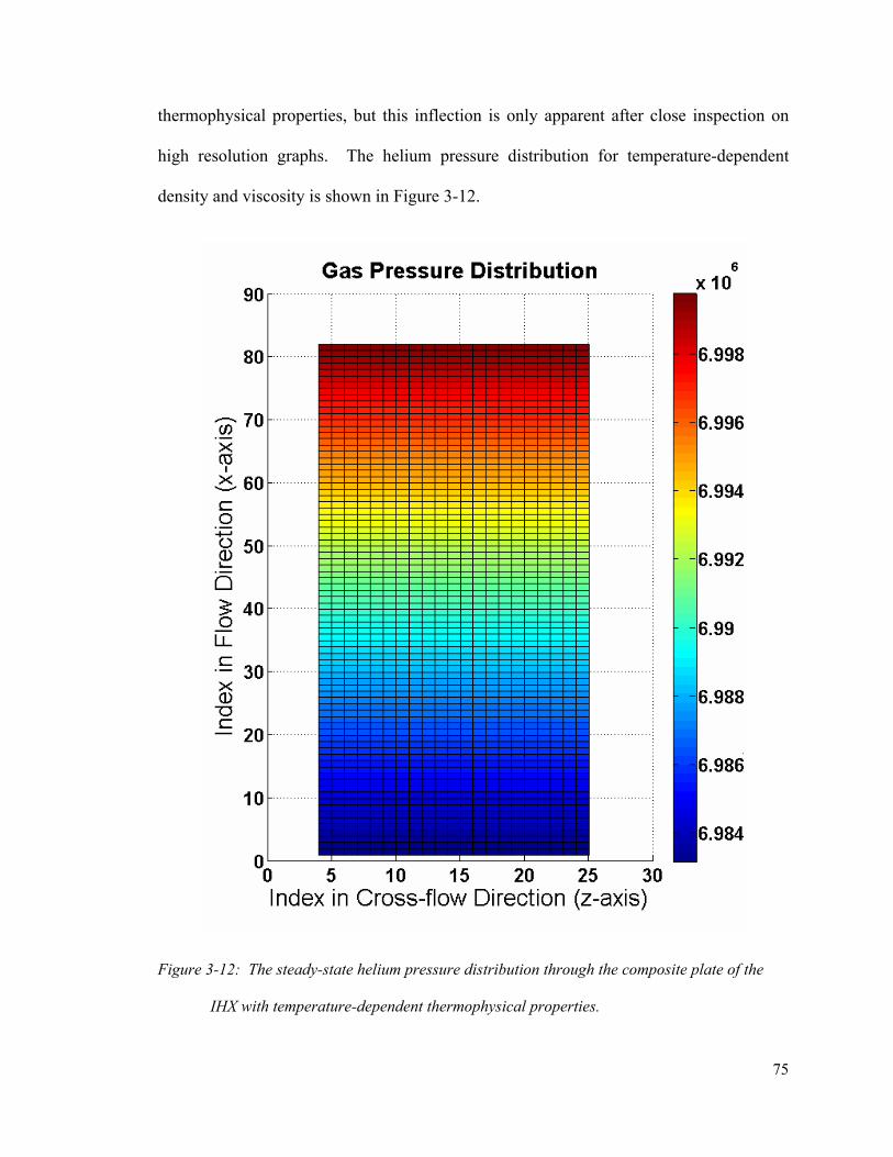
75
thermophysical properties, but this inflection is only apparent after close inspection on
high resolution graphs. The helium pressure distribution for temperature-dependent
density and viscosity is shown in Figure 3-12.
Figure 3-12: The steady-state helium pressure distribution through the composite plate of the
IHX with temperature-dependent thermophysical properties.

76
3.3.4 Liquid Speed Distribution
The complex liquid side pressure distribution drives flow through the different
permeability zones on the liquid side of the composite plate. The inlet is shown near
coordinate (0,0) and the outlet lies near coordinate (75,30). Summing the x- and z-
direction at every mesh provides a non-directional total fluid speed distribution in the
liquid plate of the IHX. The liquid flow distribution in the composite plate is shown in
Figure 3-13.
Figure 3-13: Flow speed distribution of liquid salt through the composite plate of the IHX with
temperature-dependent thermophysical properties.
77
The flow rate through the OSF region is flat and relatively constant throughout the
width of the IHX. Some peaks are visible where the inlet flow distribution channels turn
90° from the cross-flow direction to the flow direction. This is because the width of the
zone containing the flow distribution channels in the cross-flow direction is narrower
than the flow area in the primary flow direction. The step change in cross-sectional area
causes some flow channels to narrow abruptly and then expand again at the border
between zones, creating a localized nozzling effect. At the entrance to the OSF region
the liquid can be seen to increase its speed in the vicinity of the inside corner of each flow
section as it flows preferentially through the path of least resistance (in this case the
shortest path being that which hugs the corner).

78
3.3.5 Gas Speed Distribution
The flow speed distribution of helium in the composite plate is shown in Figure 3-14.
Figure 3-14: Flow speed distribution of gas through the composite plate of the IHX with
temperature-dependent thermophysical properties.
The flow speeds on the gas side are indicated as negative because they flow counter
to the direction of the coordinates and in counter-flow with the liquid salt. The effect of
temperature-dependent thermophysical properties on the flow field is mild but noticeable

79
nonetheless. The flow speed can be seen to increase by as much as 30% as the specific
volume of helium increases with rising temperatures in the helium flow. The increase in
speed would result in an increase in the Nusselt number of the flow and in increased heat
transfer; but this effect is not included in this simulation because a constant Nusselt
number is assigned based on an average flow velocity.
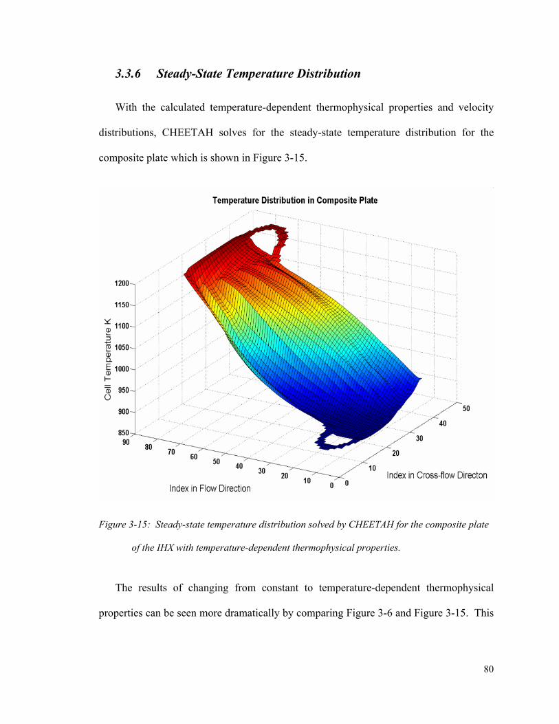
80
3.3.6 Steady-State Temperature Distribution
With the calculated temperature-dependent thermophysical properties and velocity
distributions, CHEETAH solves for the steady-state temperature distribution for the
composite plate which is shown in Figure 3-15.
Figure 3-15: Steady-state temperature distribution solved by CHEETAH for the composite plate
of the IHX with temperature-dependent thermophysical properties.
The results of changing from constant to temperature-dependent thermophysical
properties can be seen more dramatically by comparing Figure 3-6 and Figure 3-15. This
81
illustrates the significance of including this effect when determining the performance of a
compact heat exchanger over a large temperature change. While the significant effects of
temperature-dependent thermophysical properties are unique to applications that use
fluids with relatively low volumetric heat capacity, the inclusion of these effects always
result in more complex flow distributions. This effect seems particularly important when
gases are used as coolants (such as in high temperature helium-cooled modular reactors)
because local hot spots increase the gas viscosity and therefore decrease the flow in that
area. Effective simulation pertaining to the safety and efficiency of thermal equipment
involving gas coolants depends on the inclusion of temperature-dependent
thermophysical properties.
82
Chapter 4
Verification of Numerical Method
Modeling the transient response of a three-phase system in two spatial dimensions
undergoing changes in flow rate represents a problem too complex to approach
analytically. The lack of an analytical solution implies that numerical and experimental
methods are the remaining tools available to model this system. The implementation of
an explicit scheme such as that used in CHEETAH requires some comparison to verify
the results. With neither experimental nor analytical results for comparison, the validity
of the results obtained for such a complex problem remains in question. To address
questions concerning the accuracy of the numerical approach and results, a simpler
problem is first considered.
4.1 Verifying Steady-State Temperature Distribution
In order to address this important question, a simplified version of the code called
CHEETAH Cub was made to analyze a simpler system that only involves flow in one
spatial dimension, but that like the original IHX system deals with both the steady-state
and transient response of a two-fluid heat exchanger in a counter-flow arrangement. The
steady-state solution to this one-dimensional three-phase problem is solved analytically

83
and also numerically with CHEETAH Cub. The simplified system for the steady-state
analysis is shown in Figure 4-1, below.
Figure 4-1: Schematic of the two single-phase fluid heat exchanger analyzed analytically and
with CHEETAH Cub to obtain the steady-state temperature distribution.
The analytical and numerical results for this problem are presented so that the
methods and algorithms used in the two-dimensional CHEETAH code can be verified for
the steady-state case. The analytical solution to the steady-state temperature profiles in
the three phases were analyzed using the effectiveness-NTU (number of transfer units)
technique [17,18,19]. The complete analysis is available in Appendix C. The steady-
state numerical solution found with CHEETAH Cub and the analytical results for the
temperature distributions in all three phases in the heat exchanger are in agreement and
are shown in Figure 4-2.
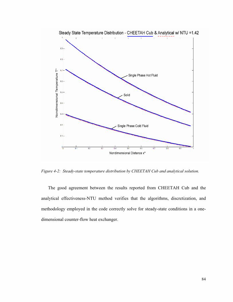
84
Figure 4-2: Steady-state temperature distribution by CHEETAH Cub and analytical solution.
The good agreement between the results reported from CHEETAH Cub and the
analytical effectiveness-NTU method verifies that the algorithms, discretization, and
methodology employed in the code correctly solve for steady-state conditions in a one-
dimensional counter-flow heat exchanger.
85
4.2 Verifying Transient Temperature Distribution
Verifying the results for the transient response in this simplified arrangement is more
complicated, but some analytical approaches are found in the literature and can be used
for comparison with results from CHEETAH Cub. An integral method approach for the
transient response is chosen for comparison; this approach is published in the
International Journal of Heat and Mass Transfer authored by Juan Yin and Michael
Jensen in 2003 [21].
In this publication, Yin and Jensen propose an analytical model for transient heat
exchanger response for a flow arrangement very similar the one considered in the steady-
state verification. This flow arrangement utilizes a single-phase fluid flowing in the
positive x direction and a constant-temperature fluid flowing in the negative x direction as
shown in the figure below. A solid wall separates the two fluids and has a prescribed
convection coefficient on each side which governs heat transfer. Because one fluid
undergoes no change temperature its flow direction is not relevant, and thus the analysis
is equally applicable to a counter-flow, cross-flow, or parallel flow heat exchanger [21].
All temperatures are averaged or lumped in the vertical direction for each phase, as
shown in Figure 4-3.

86
Figure 4-3: Schematic of heat exchanger used for verification with results from Yin and Jensen.
Yin and Jensen identify three important non-dimensional parameters that characterize
the system in their article as shown below.
1w pw
s ps
m cN
m c= , 2
c c
ps
h ANmc
= , and 3s s
ps
h ANmc
= Equation 4-1
Here, N1 shows the ratio of thermal energy that is stored in the wall and in the single
phase for each degree of temperature rise with respect to time between them. N2
represents the ratio of convection heat transfer in the constant temperature (or constant
phase) fluid to advective heat transfer in the single-phase fluid. N3 represents the ratio of
convection heat transfer associated with the single-phase fluid and the advective heat
transfer in the single-phase fluid. Finally, the NTU represents the ratio of the convective
power between a fluid and the heat exchanger per degree of temperature difference to the

87
advective power per degree of temperature change the fluid. For this problem, the NTU is
expressed as follows:
2 3
2 3( )c c s s
ps c c s s
h A h A N NNTUmc h A h A N N
= =+ + Equation 4-2
For comparison and verification the same simplified system is also characterized in
CHEETAH Cub, where an energy balance is performed on the finite volumes just as in
CHEETAH. The energy equation is written for each phase in the system occupying a
control volume. The method and algorithms are identical to those used in the CHEETAH
code for the two-dimensional system. The energy equations that represent the system are
as follows:
Constant Temperature Fluid (c):
cT Constant= (step changes in value at time equals 0) Equation 4-3
Wall or Solid (w):
( ) ( ) wc c c w s s w s w w
dTh a T T h a T T cdt
ρ′ ′− − − = Equation 4-4
Single Phase Fluid (s):
( ) ss s s s s s s s s s s w s sx x x
dTu c T u c T h a T T cdt
ρ ρ ρ+Δ
′− − − = Equation 4-5

88
In Yin and Jensen’s analysis conduction effects will be neglected for both fluids and
along the length of the wall, so the same is done in CHEETAH Cub and thus there are no
axial conduction terms in the above energy equations.
Yin and Jensen then solve for the transient response of this system analytically using
the integral method. They begin with a temperature distribution given by steady-state
operation which is obtained from an analytical model based on the set of system
parameters identified above. Two types of transients are induced:
Case 1: Step change in temperature of the uniform (constant) temperature fluid Tc
(physically this can represent the change in the saturation temperature resulting from a
step change in pressure).
Case 2: Step change in the flow rate of the single-phase fluid (physically this could
result from a sudden partial blockage in system, pump failure or valve actuation).
Temperature profiles along the length of the one-dimensional heat exchanger are
solved as a function of time. The integral method employed by Yin and Jensen involves
using the steady-state solutions before and at the end of the transients together with two
time functions to find the transient distributions for both the single-phase fluid and the
wall temperature distributions in between these two states.
Yin and Jensen’s method is analytical in nature; the derivation and final equations are
quite involved and thus will it will not be covered in any greater detail here. Instead, this
study focuses on comparing the results for CHEETAH Cub to those found by Yin and
Jensen’s model.

89
4.2.1 Case 1: Step Change in Temperature of
Uniform-Temperature Fluid
In Case 1 as presented by Yin and Jensen, the constant-temperature fluid undergoes a
step temperature rise and the transient behavior of both the single-phase fluid and the
wall are calculated. Yin and Jensen used the object-oriented Modelica language to
program a simulation in the Dymola (Dynamic Modeling Laboratory) software to verify
their integral method analysis [21].
Figure 4-4 shows the results from the CHEETAH Cub code, Yin and Jensen’s
integral method analysis, and Yin and Jensen’s computational Dymola model. The three
analyses show excellent agreement throughout the transient for the single-phase fluid.
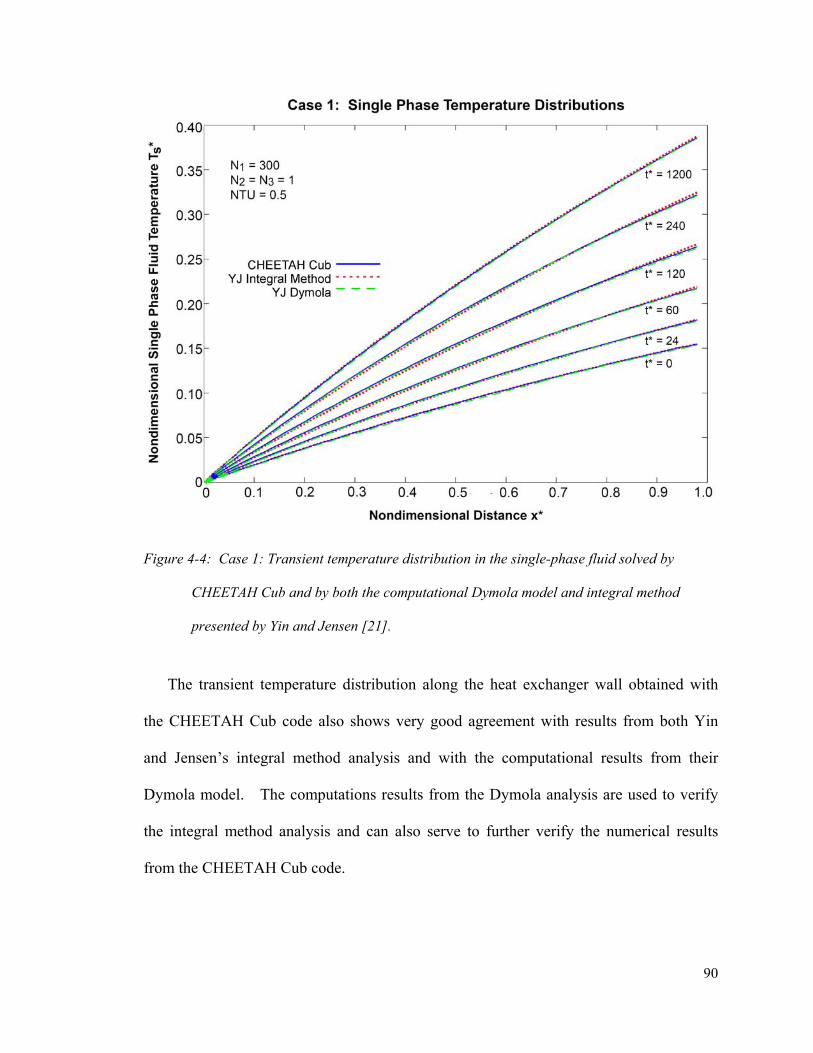
90
Figure 4-4: Case 1: Transient temperature distribution in the single-phase fluid solved by
CHEETAH Cub and by both the computational Dymola model and integral method
presented by Yin and Jensen [21].
The transient temperature distribution along the heat exchanger wall obtained with
the CHEETAH Cub code also shows very good agreement with results from both Yin
and Jensen’s integral method analysis and with the computational results from their
Dymola model. The computations results from the Dymola analysis are used to verify
the integral method analysis and can also serve to further verify the numerical results
from the CHEETAH Cub code.
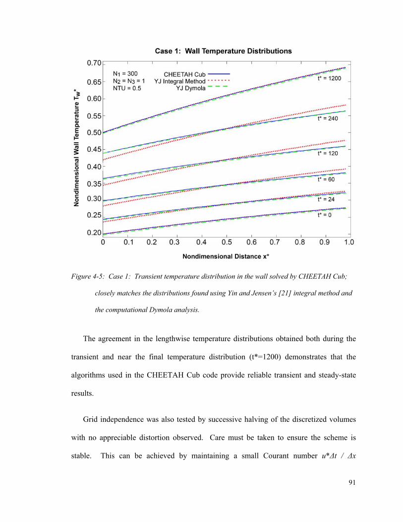
91
Figure 4-5: Case 1: Transient temperature distribution in the wall solved by CHEETAH Cub;
closely matches the distributions found using Yin and Jensen’s [21] integral method and
the computational Dymola analysis.
The agreement in the lengthwise temperature distributions obtained both during the
transient and near the final temperature distribution (t*=1200) demonstrates that the
algorithms used in the CHEETAH Cub code provide reliable transient and steady-state
results.
Grid independence was also tested by successive halving of the discretized volumes
with no appreciable distortion observed. Care must be taken to ensure the scheme is
stable. This can be achieved by maintaining a small Courant number u*Δt / Δx
92
(CoMAX <.25 was used in this case). Again, this verification effort (Case 1) is related to
the transient step change in temperature of the uniform temperature fluid.
In this section, the algorithms in CHEETAH Cub are tested against the transient
behavior that would result in the heat exchanger during a thermal transient induced by a
step change in the temperature of the uniform temperature fluid. The study by Yin and
Jensen contains an analytical model that is verified by numerical simulation. Both results
presented the analyses by Yin and Jensen showed excellent agreement with the results
obtained by the CHEETAH Cub code.
4.2.2 Case 2: Step Change in Flow Rate of Single-Phase Fluid
In Case 2, gamma (γ) represents the ratio of mass flow rate of the single-phase fluid
after the step change to the mass flow rate of the single-phase fluid before the step
change. The following figures show the fidelity of the CHEETAH Cub code under flow
transients of varying magnitude. To match the results published by Yin and Jensen,
rather than showing the spatial temperature distribution, the following figures show the
variation in time of the outlet temperature under different flow transients denoted by
varying values of gamma, / om mγ ∞= . This allows a more complete comparison of the
transient effects over various flow transients.
The results from the CHEETAH Cub code are compared with results from Yin and
Jensen in Figure 4-6.
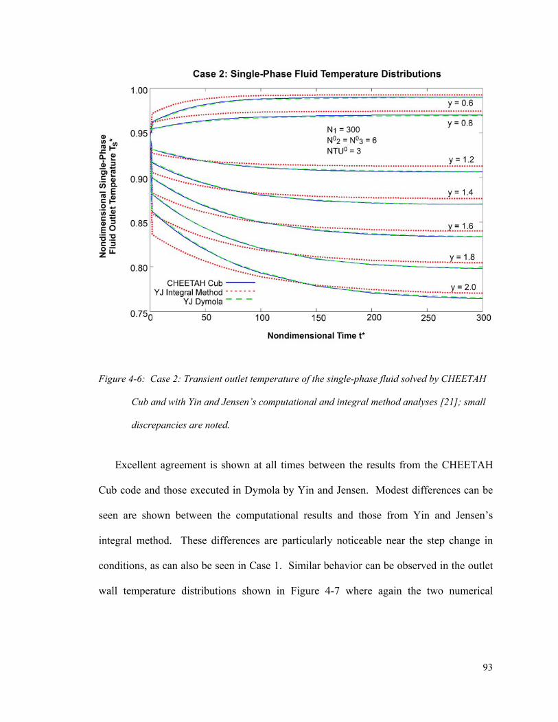
93
Figure 4-6: Case 2: Transient outlet temperature of the single-phase fluid solved by CHEETAH
Cub and with Yin and Jensen’s computational and integral method analyses [21]; small
discrepancies are noted.
Excellent agreement is shown at all times between the results from the CHEETAH
Cub code and those executed in Dymola by Yin and Jensen. Modest differences can be
seen are shown between the computational results and those from Yin and Jensen’s
integral method. These differences are particularly noticeable near the step change in
conditions, as can also be seen in Case 1. Similar behavior can be observed in the outlet
wall temperature distributions shown in Figure 4-7 where again the two numerical
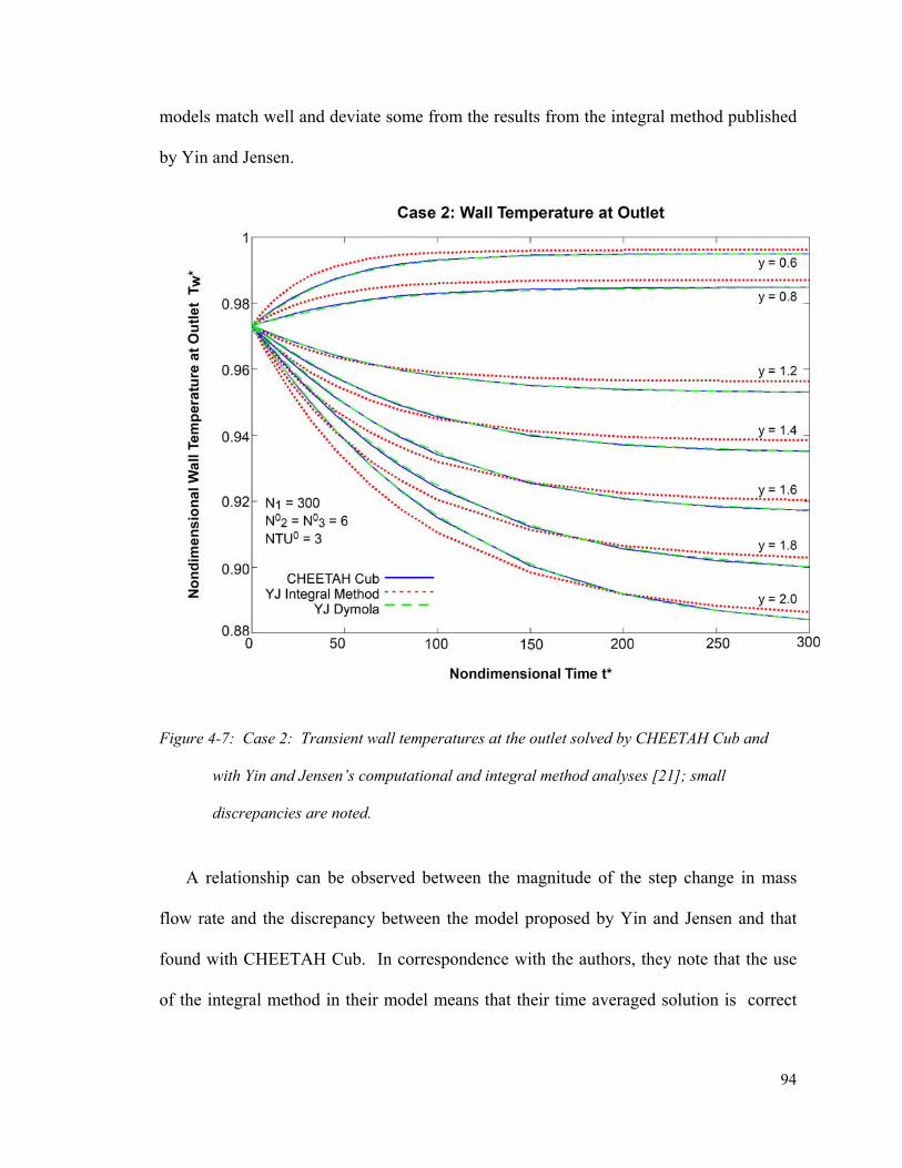
94
models match well and deviate some from the results from the integral method published
by Yin and Jensen.
Figure 4-7: Case 2: Transient wall temperatures at the outlet solved by CHEETAH Cub and
with Yin and Jensen’s computational and integral method analyses [21]; small
discrepancies are noted.
A relationship can be observed between the magnitude of the step change in mass
flow rate and the discrepancy between the model proposed by Yin and Jensen and that
found with CHEETAH Cub. In correspondence with the authors, they note that the use
of the integral method in their model means that their time averaged solution is correct
95
but that it will show greater error at times near the initiation of the transient. In Case 2,
the discrepancy is indeed most notable at times near the initiation of the transient and is
mostly limited to the single-phase temperature distribution (Figure 4-6) since it
experiences a more volatile change in temperature from the high value of N1 and due to
the N3 value being greater than unity. Comparing the single-phase fluid and wall
temperature histories reported by CHEETAH Cub with those found in the numerical
model simulated in Dymola by Yin and Jensen, it is clear that both numerical models
produce matching results.
In the numerical analysis, Yin and Jensen checked grid independence in space and
time by successive halving of the increments [21]. Furthermore, Yin and Jensen
benchmarked their numerical results against those of Romie [22] and Roetzel and Xuan
[23] for a parallel and counter-flow heat exchanger arrangement and reported that “the
agreement was excellent [21].” The near match between the results of the CHEETAH
Cub code and those from the Dymola analysis performed by Yin and Jensen verifies the
approach used in CHEETAH Cub. The good agreement with Yin and Jensen’s integral
method further verifies both analyses. These results from this one-dimensional transient
analysis give confidence in the techniques implemented in the two-dimensional
CHEETAH code, since it relies on the same method and algorithms.
96
Chapter 5
Thermomechanical Stress Analysis
5.1 Domain Sub-Structuring with Effective Mechanical Properties
The creation of the composite plate is critical to both the mechanical analysis and the
thermal hydraulic analysis. The thermal hydraulic results from Chapter 3 are buttressed
by the verification of the code and method in Chapter 4. This is important because the
thermomechanical stress analysis that follows will rely on temperature distributions
provided by CHEETAH and presented earlier.
Just as discretizing the plate at the fin-scale required prohibitive computational power
in the thermal hydraulic analysis, so too is it unfeasible to discretize at the fin scale in
analyzing plate-scale temperature distributions on the composite plate. In the thermal
hydraulic analysis it is valuable to use volume-averaged properties such as effective
permeability, porosity, and effective convection coefficients. In a similar fashion, the
evaluation of volume-averaged mechanical properties in zones within the composite plate
will enable mechanical analysis on the plate scale with moderate computational time.
Effective mechanical properties such as Poisson ratios, elastic, and shear moduli will be
determined for several regions in the composite plate that share complex geometries such
as the solid plate, flow distributor regions, and the offset strip fin region. The regions for

97
which effective mechanical properties are evaluated as well as the regional representative
unit cells are shown around the composite plate in Figure 5-1, below.
Figure 5-1: Composite plate with the representative unit cells that are used to calculate
effective mechanical properties.
Finding the effective mechanical properties of a complex and repeating geometry
involves subjecting a test section or unit cell to the same test procedures used to
characterize a material. Essentially, the complex repeating geometry of the region is
replaced by a simple geometry made of a representative material that has the same
mechanical properties as the complex geometry in another material. This concept is

98
illustrated in Figure 5-2, below, where Bar 1 and Bar 2 are both made of Alloy A while
Bar 3 is made out of a more elastic Alloy B. Both Bar 1 and Bar 3 are solid while Bar 2
has a complex repeating geometry.
Figure 5-2: A mechanical component with a simple geometry can replace a component
with a complex geometry when the two share effective mechanical properties such
as an effective modulus of elasticity.
Under the same compressive load, both Bar 2 and Bar 3 deflect equally and both deflect
more than Bar 1. Analyzing the deflection and applied load allows for the calculation of
a modulus of elasticity (E) for each bar. Clearly, Bar 1 and Alloy A will have the highest
modulus of elasticity (most rigid). The more complex geometry of Bar 2 with Alloy A
gives it an effective elastic modulus (E2A) that equals the elastic modulus (E3B) for the
less rigid Bar 3 and Alloy B. This means that in this type of model the more complex
geometry of Bar 2 with Alloy A can be replaced by the simpler geometry of Bar 3 with
Alloy B, saving computation time.
99
Explained more conceptually, the idea of effective properties and materials in a
computational model is analogous to replacing the complex geometry of a short metal
spring with the simple geometry of a short rubber cylinder or slug that has the same
elasticity. Clearly the short rubber cylinder is simpler to model from a computational
perspective due to its simple geometry.
Applying this idea to the composite plate shown in Figure 5-1, above, the unique
geometry of each of the four representative unit cells in the composite plate will create
four regions in the composite plate, each with their own effective mechanical properties,
as if the regions were made of different materials. Unlike in the one-dimensional and
isotropic example shown above, however, three out of the four unit cells have orthotropic
material properties. The isotropic cell is unit cell A while the orthotropic unit cells are B,
C, and D.
Explained simply, orthotropic materials have mechanical properties that are
directionally-dependent in the three principle axes. Characterizing the effective material
properties of each of the regions with orthotropic unit cells will require nine material
constants per unit cell versus two material constants needed to fully characterize the
isotropic unit cell. Detailed work on this technique can be found in a publication by D.
Huang, H. Zhao, and P. F. Peterson [2] and in a descriptive write-up by Kenneth Lee
[Appendix D], who found the effective mechanical properties in this study.
The nine constants needed to characterize an orthotropic material include three-
directional moduli of elasticity (Young’s moduli), E, three Poisson’s ratios (relate strain
in orthogonal directions), ν, and three shear moduli, G. These constants are related to one
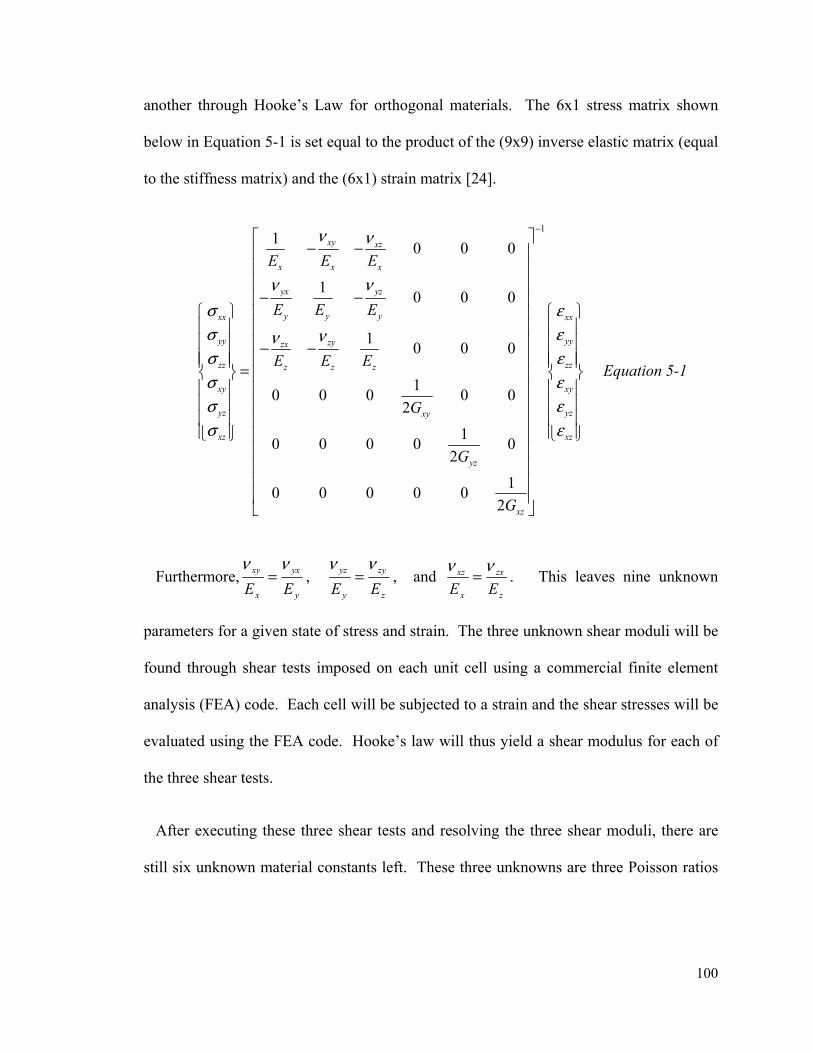
100
another through Hooke’s Law for orthogonal materials. The 6x1 stress matrix shown
below in Equation 5-1 is set equal to the product of the (9x9) inverse elastic matrix (equal
to the stiffness matrix) and the (6x1) strain matrix [24].
11 0 0 0
1 0 0 0
1 0 0 0
10 0 0 0 02
10 0 0 0 02
10 0 0 0 02
xy xz
x x x
yx yz
y y yxx xx
yy yyzyzx
zz zzz z z
xy xy
yz yzxy
xz xz
yz
xz
E E E
E E E
E E E
G
G
G
ν ν
ν νσ εσ εννσ εσ εσ εσ ε
−⎡ ⎤
− −⎢ ⎥⎢ ⎥⎢ ⎥− −⎢ ⎥
⎧ ⎫ ⎧ ⎫⎢ ⎥⎪ ⎪ ⎪ ⎪⎢ ⎥⎪ ⎪ ⎪ ⎪⎢ ⎥− −⎪ ⎪ ⎪ ⎪⎢ ⎥⎪ ⎪ ⎪ ⎪=⎨ ⎬ ⎨ ⎬⎢ ⎥⎪ ⎪ ⎪⎢ ⎥⎪ ⎪ ⎪⎢ ⎥⎪ ⎪ ⎪⎢ ⎥⎪ ⎪ ⎪⎩ ⎭ ⎩⎢ ⎥
⎢ ⎥⎢ ⎥⎢ ⎥⎢ ⎥⎣ ⎦
⎪⎪⎪⎪⎭
Equation 5-1
Furthermore,y
yx
x
xy
EEνν
= , z
zy
y
yz
EEνν
= , and z
zx
x
xz
EEνν
= . This leaves nine unknown
parameters for a given state of stress and strain. The three unknown shear moduli will be
found through shear tests imposed on each unit cell using a commercial finite element
analysis (FEA) code. Each cell will be subjected to a strain and the shear stresses will be
evaluated using the FEA code. Hooke’s law will thus yield a shear modulus for each of
the three shear tests.
After executing these three shear tests and resolving the three shear moduli, there are
still six unknown material constants left. These three unknowns are three Poisson ratios
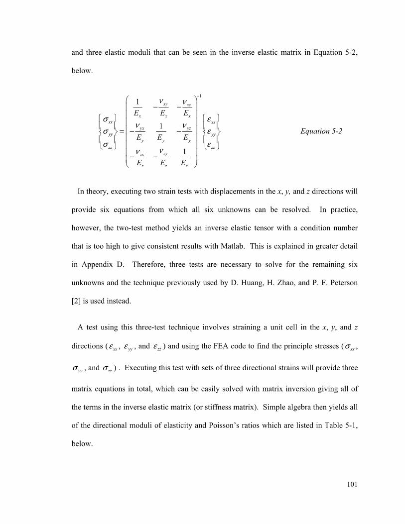
101
and three elastic moduli that can be seen in the inverse elastic matrix in Equation 5-2,
below.
11
1
1
xy xz
x x xxx xx
yx yzyy yy
y y yzz zz
zyzx
z z z
E E E
E E E
E E E
ν ν
σ εν ν
σ εσ ε
νν
−⎛ ⎞
− −⎜ ⎟⎜ ⎟⎧ ⎫ ⎧ ⎫⎜ ⎟⎪ ⎪ ⎪ ⎪⎜ ⎟= − −⎨ ⎬ ⎨ ⎬⎜ ⎟⎪ ⎪ ⎪ ⎪⎜ ⎟⎩ ⎭ ⎩ ⎭⎜ ⎟− −⎜ ⎟⎝ ⎠
Equation 5-2
In theory, executing two strain tests with displacements in the x, y, and z directions will
provide six equations from which all six unknowns can be resolved. In practice,
however, the two-test method yields an inverse elastic tensor with a condition number
that is too high to give consistent results with Matlab. This is explained in greater detail
in Appendix D. Therefore, three tests are necessary to solve for the remaining six
unknowns and the technique previously used by D. Huang, H. Zhao, and P. F. Peterson
[2] is used instead.
A test using this three-test technique involves straining a unit cell in the x, y, and z
directions ( xxε , yyε , and zzε ) and using the FEA code to find the principle stresses ( xxσ ,
yyσ , and zzσ ) . Executing this test with sets of three directional strains will provide three
matrix equations in total, which can be easily solved with matrix inversion giving all of
the terms in the inverse elastic matrix (or stiffness matrix). Simple algebra then yields all
of the directional moduli of elasticity and Poisson’s ratios which are listed in Table 5-1,
below.
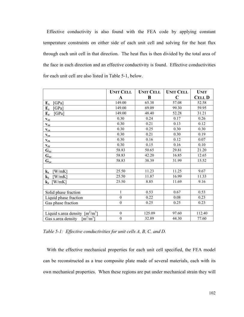
102
Effective conductivity is also found with the FEA code by applying constant
temperature constraints on either side of each unit cell and solving for the heat flux
through each unit cell in that direction. The heat flux is then divided by the total area of
the face in each direction and an effective conductivity is found. Effective conductivities
for each unit cell are also listed in Table 5-1, below.
UNIT CELL A
UNIT CELL B
UNIT CELL C
UNIT CELL D
Ex [GPa] 149.00 65.38 57.08 52.58 Ey [GPa] 149.00 69.09 99.30 59.95 Ez [GPa] 149.00 48.40 52.28 31.21 vxy 0.30 0.24 0.17 0.26 vxz 0.30 0.21 0.13 0.12 vyx 0.30 0.25 0.30 0.30 vyz 0.30 0.21 0.30 0.19 vzx 0.30 0.16 0.12 0.07 vzy 0.30 0.15 0.16 0.10 Gxy 58.83 50.65 29.81 21.20 Gxz 58.83 42.20 16.85 12.65 Gyz 58.83 38.39 31.99 15.52 kx [W/mK] 25.50 11.23 11.25 9.67 ky [W/mK] 25.50 11.87 16.99 11.33 kz [W/mK] 25.50 8.85 11.69 9.16 Solid phase fraction 1 0.53 0.67 0.53 Liquid phase fraction 0 0.22 0.08 0.23 Gas phase fraction 0 0.25 0.25 0.23 Liquid s.area density [m2/m3] 0 125.09 97.60 112.40 Gas s.area density [m2/m3] 0 32.89 44.30 77.60
Table 5-1: Effective conductivities for unit cells A, B, C, and D.
With the effective mechanical properties for each unit cell specified, the FEA model
can be reconstructed as a true composite plate made of several materials, each with its
own mechanical properties. When these regions are put under mechanical strain they will

103
respond just as the more complex geometry of the unit cells would under similar
deflection because analysis from their stress tests provide the effective moduli and
Poisson’s ratios.
After recreating the two-dimensional composite plate analyzed in CHEETAH in the
FEA code ANSYS, the effective mechanical properties are added to the code’s material
library and assigned to their respective zones as shown in Figure 5-3, below. The solid
plate, offset strip fin, flow, and cross-flow distributor areas are clearly assigned different
effective material properties as dictated by color.
Figure 5-3: Two-dimensional ANSYS model of composite plate with effective material
properties assigned.
104
5.2 CHEETAH-ANSYS Communicator Code (CAC code)
With the composite plate’s temperature distribution in CHEETAH’s Matlab data files
and the composite plate’s effective mechanical properties modeled and assigned in
ANSYS, a code, tool, or utility had to be created to communicate results between these
two codes. One of the attractive features of ANSYS versus other FEA codes is its simple
text-driven commands. ANSYS can easily read simple text files with commands in them
that allow the user to control every node and element in a finite element analysis. This
option is not available with other FEA codes that are more intensely driven from their
graphical user interface (GUI) such as Pro-E/Mechanica, Abacus, and COMSOL. The
ability to read text files with assignments to every node gives the researcher complete
control over the mechanical analysis. In this case it permits several thousand temperature
results from CHEETAH to be entered into over ten thousand nodes in the FEA model in
ANSYS. With matrices involving tens of thousands of values, this work must be
automated.
Automating the data processing from CHEETAH to ANSYS first requires exporting a
node text file from ANSYS containing the node number, and x, y, z coordinates of each
structural node in the composite plate model (just over 10,000 nodes). This requires
going to ANSYS’ Preprocessor>Modeling>Create>Nodes>Write Node File commands
and naming the file. This file is then read into the CHEETAH-ANSYS Communicator
code (CAC code) written in Matlab. The data file from CHEETAH is also loaded into
the CAC code where algorithms calculate the position of each ANSYS node on the
CHEETAH discretization or grid. With the ANSYS node’s location, the distance to the
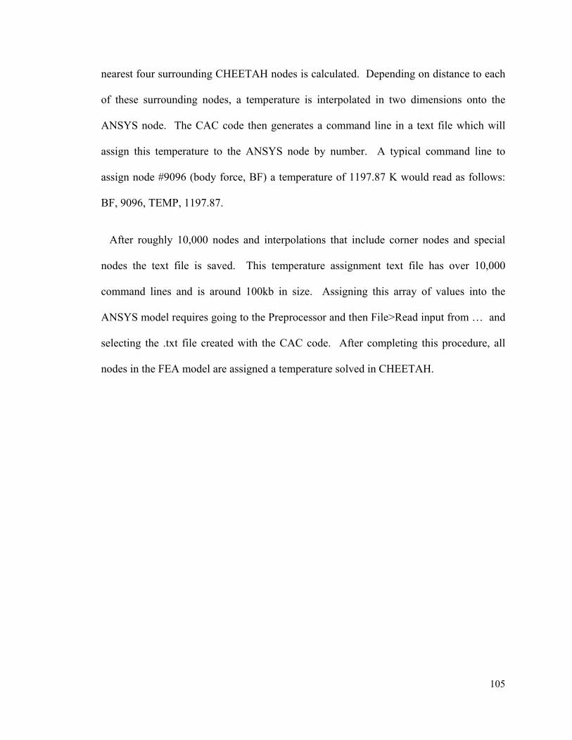
105
nearest four surrounding CHEETAH nodes is calculated. Depending on distance to each
of these surrounding nodes, a temperature is interpolated in two dimensions onto the
ANSYS node. The CAC code then generates a command line in a text file which will
assign this temperature to the ANSYS node by number. A typical command line to
assign node #9096 (body force, BF) a temperature of 1197.87 K would read as follows:
BF, 9096, TEMP, 1197.87.
After roughly 10,000 nodes and interpolations that include corner nodes and special
nodes the text file is saved. This temperature assignment text file has over 10,000
command lines and is around 100kb in size. Assigning this array of values into the
ANSYS model requires going to the Preprocessor and then File>Read input from … and
selecting the .txt file created with the CAC code. After completing this procedure, all
nodes in the FEA model are assigned a temperature solved in CHEETAH.
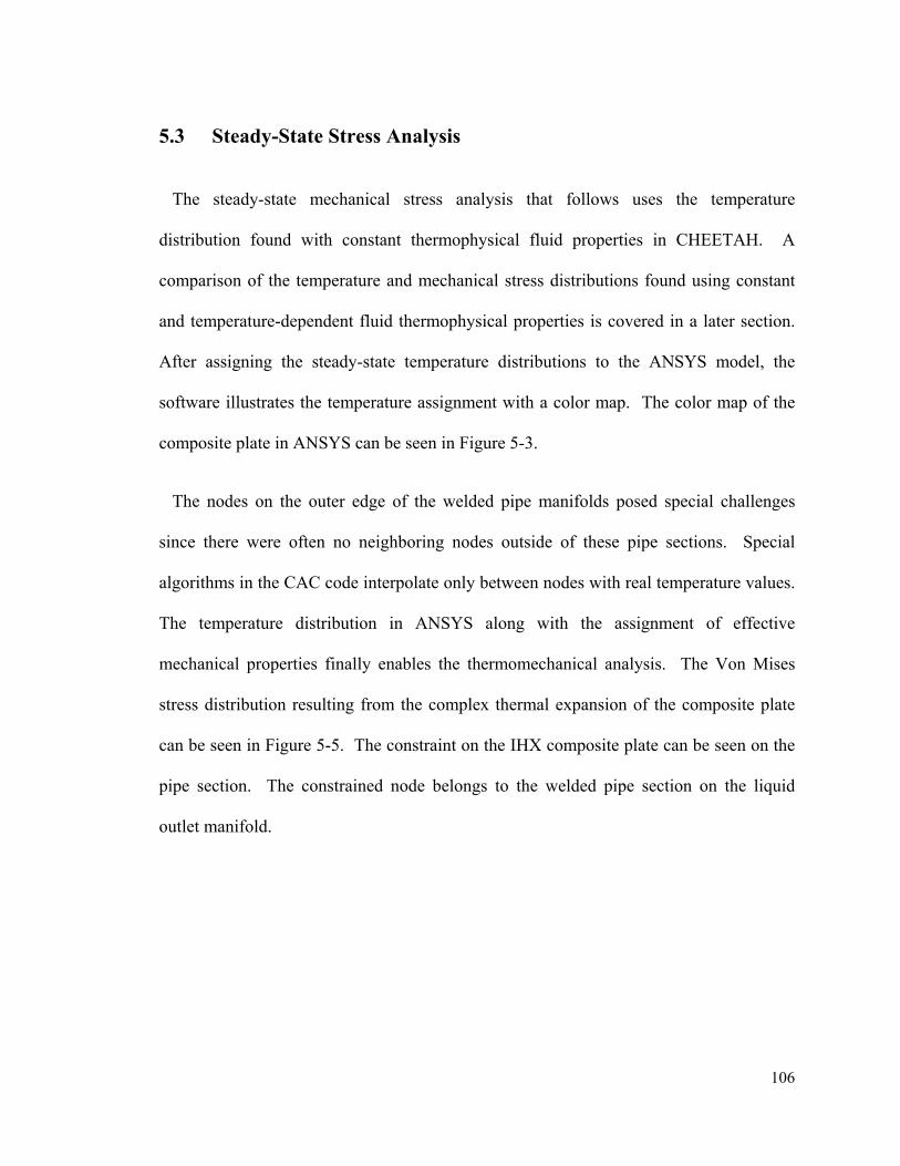
106
5.3 Steady-State Stress Analysis
The steady-state mechanical stress analysis that follows uses the temperature
distribution found with constant thermophysical fluid properties in CHEETAH. A
comparison of the temperature and mechanical stress distributions found using constant
and temperature-dependent fluid thermophysical properties is covered in a later section.
After assigning the steady-state temperature distributions to the ANSYS model, the
software illustrates the temperature assignment with a color map. The color map of the
composite plate in ANSYS can be seen in Figure 5-3.
The nodes on the outer edge of the welded pipe manifolds posed special challenges
since there were often no neighboring nodes outside of these pipe sections. Special
algorithms in the CAC code interpolate only between nodes with real temperature values.
The temperature distribution in ANSYS along with the assignment of effective
mechanical properties finally enables the thermomechanical analysis. The Von Mises
stress distribution resulting from the complex thermal expansion of the composite plate
can be seen in Figure 5-5. The constraint on the IHX composite plate can be seen on the
pipe section. The constrained node belongs to the welded pipe section on the liquid
outlet manifold.
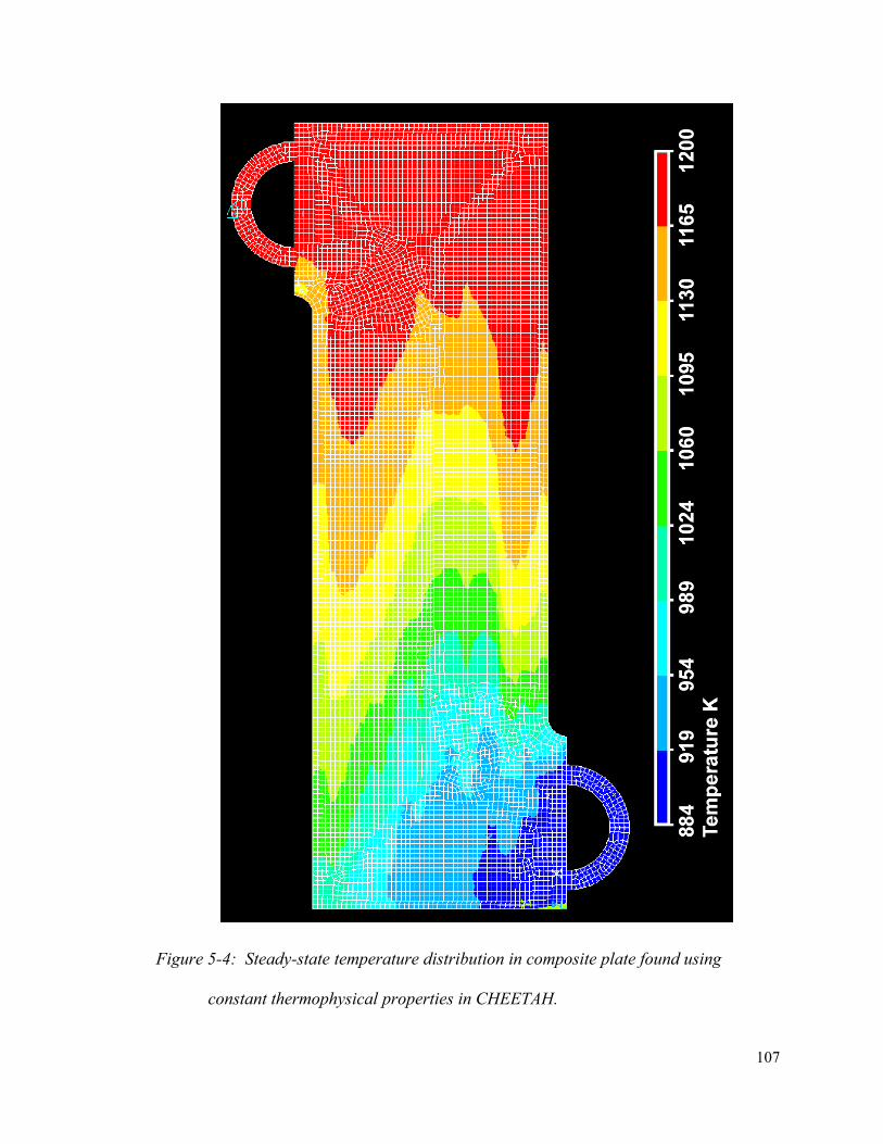
107
Figure 5-4: Steady-state temperature distribution in composite plate found using
constant thermophysical properties in CHEETAH.
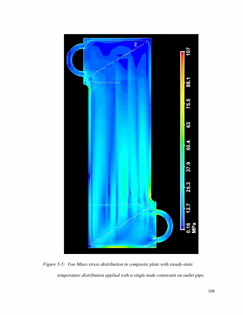
108
Figure 5-5: Von Mises stress distribution in composite plate with steady-state
temperature distribution applied with a single node constraint on outlet pipe.
109
5.3.1 Failure Analysis - Yielding
The primary failure modes explored in this work are yielding and creep. At the plate
scale the Von Mises stress distribution provided in Figure 5-5 is used to judge failure
based on yielding, the onset of plastic deformation. The mechanical properties of Alloy
617 (Inconel) are published by HAYNES International [25]. The yield stress is a strong
inverse function of temperature at high temperatures. Haynes reports that at 1143 K
(870°C) the yield stress of Alloy 617 is 207 MPa, while at 1253 K (980°C) the yield
stress is 111 MPa. The peak operating temperatures in the IHX are 1200 K (927°C), and
performing a linear interpolation gives a yield stress at this temperature of 157 MPa.
Assuming a typical factor of safety of two means that stresses in the composite plate
should not exceed 78 MPa.
It is important to emphasize that the true yield stress of the composite plate is
temperature dependent and because there is a spatial temperature distribution on the plate
the yield stress is therefore spatially dependent. This is due to the large temperature
difference from one end of the plate to the other, and also because the yield stress vary
greatly with temperature.
For the steady-state temperature distribution, the peak stresses on the plate scale are
around 100 MPa. This is below the yield stress but above the design limit set at 78 MPa.
However, peak stresses do occur far from peak temperatures which are located near the
gas inlet as can be seen in Figure 5-4. From the perspective of mechanical yielding, it
seems the composite plate can withstand the operational stresses if imposed momentarily,
110
but the current design for the composite plate fails to provide an adequate factor of safety.
The following creep analysis will further explore the effects of this stress distribution on
the composite plate over an extended period of time.
5.3.2 Failure Analysis - Creep
The Von Mises stress distribution provides the basis for the creep failure analysis
performed on this design of the composite plate in the IHX. By operating at peak
temperatures of 1200 K (927°C), the IHX must be robust enough to endure the stresses
imposed at the operating procedure over a 30 year life. Several high-temperature alloys
have creep data available for 100,000 hours, but for Alloy 617 only results for 10,000
hours were found. The maximum allowable creep stress listed by HAYNES International
[25] at 1143 K (870°C) is 47 MPa, while at 1253 K (980°C) the maximum allowable
creep stress drops to 17.45 MPa. The peak operating temperatures in the IHX are 1200 K
(927°C), and performing a linear interpolation gives a maximum allowable sustained
creep stress of 32.34 MPa. Including a factor of safety of two, the design limit for creep
stress is 16 MPa for this application of Inconel Alloy 617.
In Figure 5-5, above, the peak stresses in the composite plate certainly exceed the
design creep limit of 16 MPa. Operating Von Mises stresses in this two-dimensional
analysis shows that the areas of the IHX exposed to peak temperatures experience
operating stresses around 25 MPa which already surpasses the design limit for creep
111
stress. Furthermore, it is important to note that this analysis includes only plate-scale
expansion stresses and therefore excludes the pressure differential between the liquid and
gas phases. This pressure differential is 7MPa, so with the plate-scale stresses included
the total stress could come close to the maximum allowable creep stress with no safety
factor. Plate-scale creep stresses in this design are unacceptable for the application; the
composite plate must be redesigned to reduce operational stresses. This indicates that
fin-scale stresses, which tend to be higher, will likely fail the creep criteria as well.
5.4 Effect of Constant and Temperature-Dependent Thermophysical Fluid Properties
Two complete steady-state thermal, hydraulic, and mechanical stress analyses were
executed using the CHEETAH code and the FEA code ANSYS. The objective is to
understand the significance of including effects caused by temperature-dependent
thermophysical fluid properties in the analysis. Therefore both analyses used the same
boundary conditions and composite plate parameters and were only different in that one
used constant thermophysical fluid properties while the other included the temperature
dependency. The resulting steady-state temperature distributions from both analyses are
shown in Figure 5-6; the corresponding Von Mises stress distributions for both analyses
are shown in Figure 5-7 and Figure 5-8.
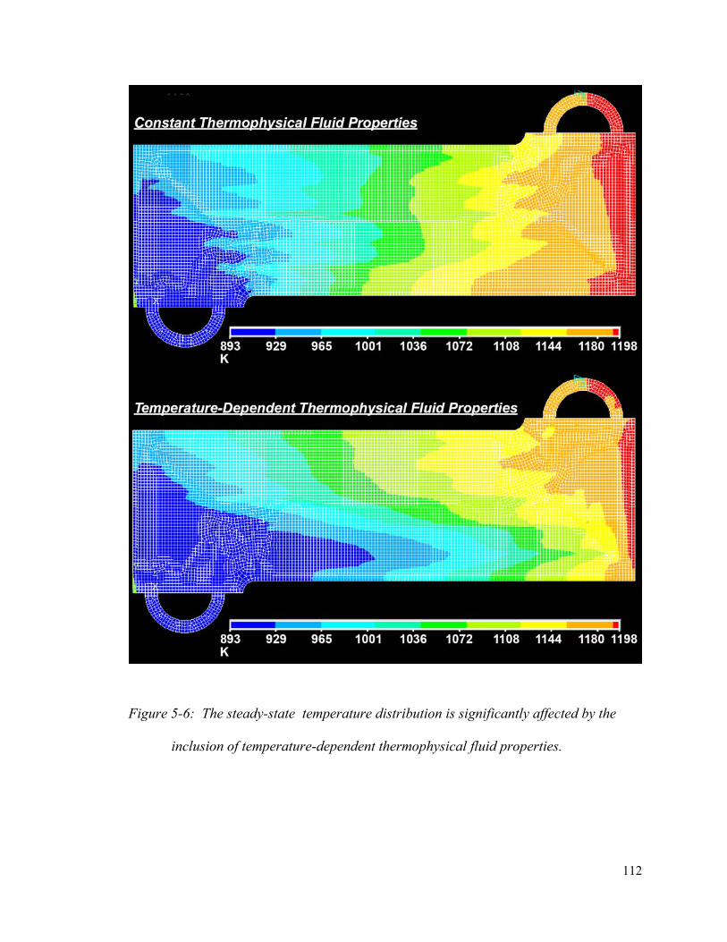
112
Figure 5-6: The steady-state temperature distribution is significantly affected by the
inclusion of temperature-dependent thermophysical fluid properties.
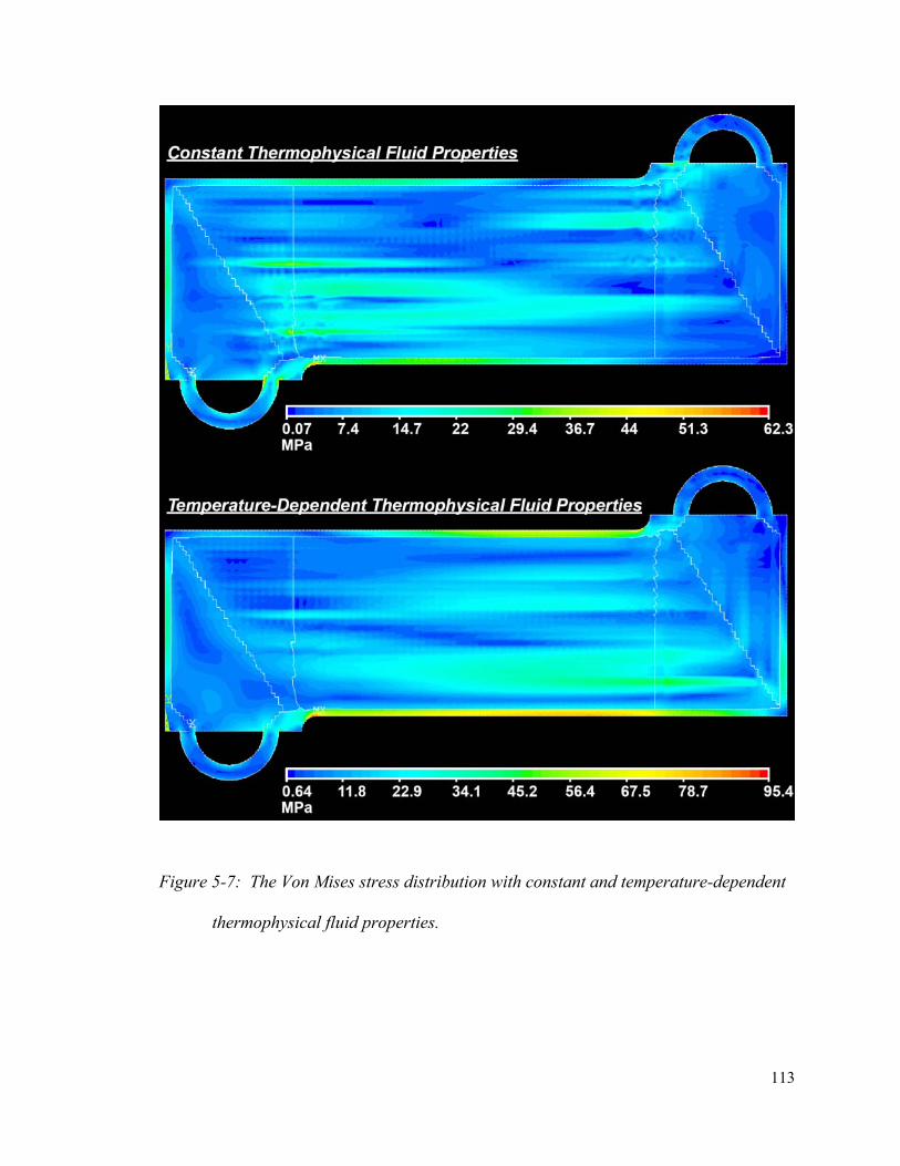
113
Figure 5-7: The Von Mises stress distribution with constant and temperature-dependent
thermophysical fluid properties.
114
The thermal results show that the temperature-dependent fluid thermophysical
properties significantly affect the temperature distribution in the composite plate. The
larger cold zone near the liquid salt (cold fluid) inlet shows that the exposure to the
longer distributor in the hot outlet manifold reduces the average viscosity of that flow
path and increases flow and thus cooling over that flow path.
The resulting mechanical stress field shown in Figure 5-7 shows that while peak
stresses increase by 50% in the temperature-dependent case, the steady-state stresses are
still sufficiently low so as to not cause yielding. The peak stresses in the temperature-
dependent fluid property case, however, are above the maximum allowable stresses when
considering the safety factor. The stress field is significantly above what could be
tolerated from a mechanical creep perspective in both cases. It is interesting to note that
the stress field over the plate does change significantly when considering the
temperature-dependent thermophysical fluid properties.
5.5 Transient Stress Analysis
The CHEETAH code, the CHEETAH-ANSYS Communicator code (CAC Code), and
the FEA code (ANSYS) have enabled the mechanical analysis of composite plate design.
The results have shown that the composite plate fails the design stress limits set for both
yield and creep stresses. Still, this is an illustrative example that aims to show how the
methodology and CHEETAH code can be applied towards compact heat exchanger
optimization by executing comprehensive thermal, hydraulic, and mechanical analysis.
115
Despite showing that a redesign of the composite plate is required based on previously
analyzed criteria, the analyses based on severe thermal hydraulic transients are presented
to illustrate the methodology and utility of the CHEETAH code.
The two transients solved by CHEETAH in Chapter 3 involve harsh step changes in the
flow of just one of the two fluids in the IHX. The following analysis will build on those
thermal hydraulic results to perform transient thermomechanical analysis on the
composite plate. The temperature distributions come from analysis using the CHEETAH
code with constant thermophysical properties. Including the steady-state temperature
distribution, a total of six temperature distributions are used in each transient analysis.
The first thermomechanical transient examined results from the interruption of the cold
liquid salt flow in the heat exchanger. Consequently a heating front propagates through
the IHX as the hot helium continues flowing. The results for the first thermomechanical
transient can be seen in Figure 5-8 in 15 second intervals. The second thermomechanical
transient examined results from the interruption of the hot helium flow in the heat
exchanger. A cooling front then moves through the IHX as the cold liquid salt continues
flowing. The results for the second thermomechanical transient can be seen in Figure
5-9. For both cases, the temperature distributions can be seen on the left-side and the
corresponding Von Mises stresses are illustrated on the right-side of Figure 5-8 and
Figure 5-9, below. One legend applies to all of the stress distributions and another to all
the temperature distributions.

116
5.5.1 Liquid Salt (Cold) Pump Trip
Figure 5-8: Temperature and Von Mises stress distributions corresponding to the liquid
salt pump trip results in heating front propagation.
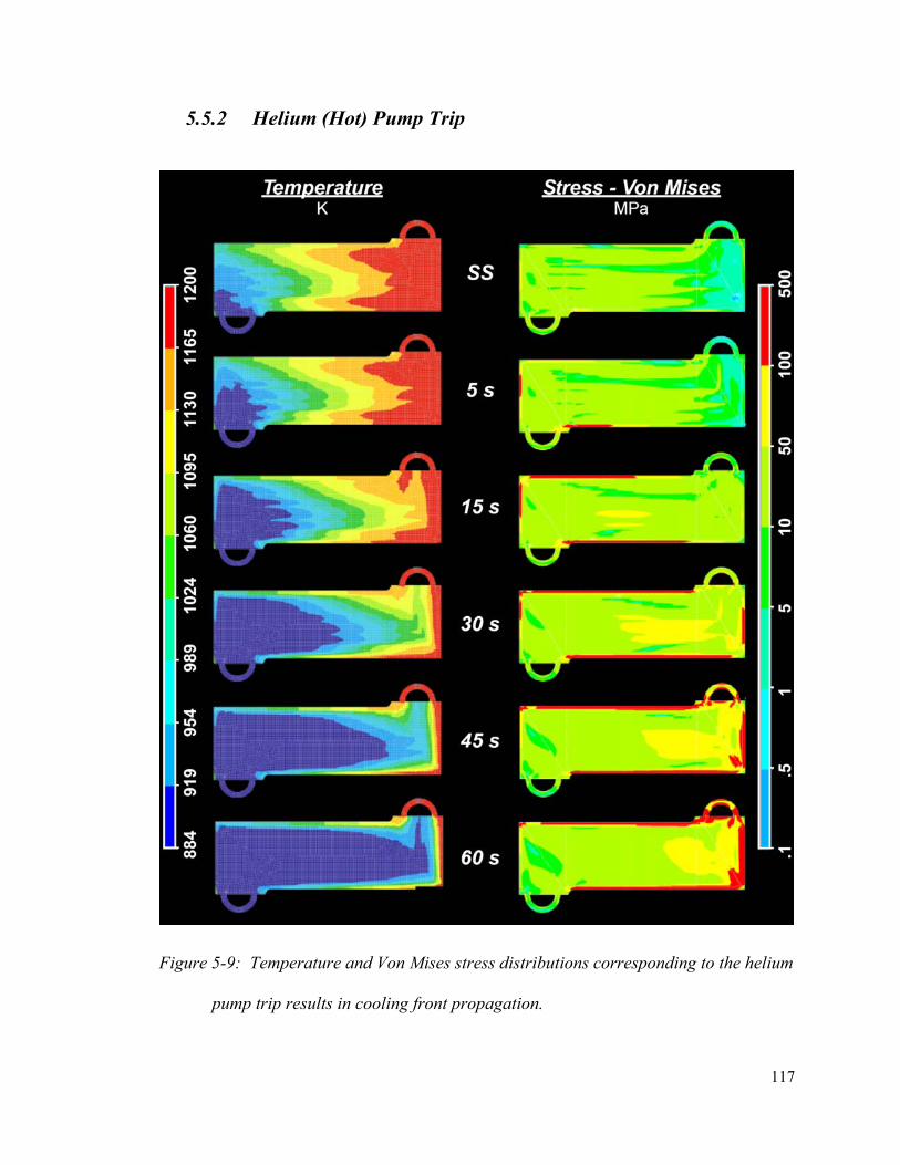
117
5.5.2 Helium (Hot) Pump Trip
Figure 5-9: Temperature and Von Mises stress distributions corresponding to the helium
pump trip results in cooling front propagation.
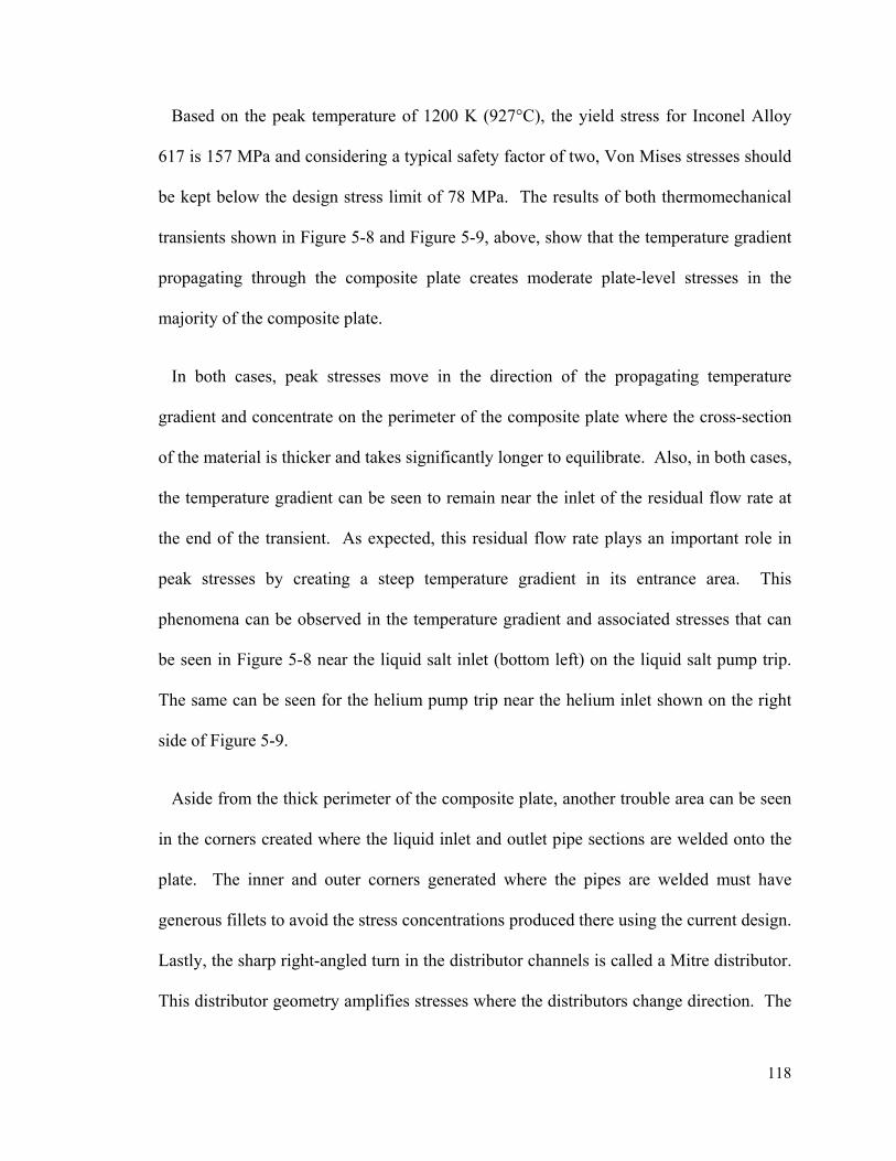
118
Based on the peak temperature of 1200 K (927°C), the yield stress for Inconel Alloy
617 is 157 MPa and considering a typical safety factor of two, Von Mises stresses should
be kept below the design stress limit of 78 MPa. The results of both thermomechanical
transients shown in Figure 5-8 and Figure 5-9, above, show that the temperature gradient
propagating through the composite plate creates moderate plate-level stresses in the
majority of the composite plate.
In both cases, peak stresses move in the direction of the propagating temperature
gradient and concentrate on the perimeter of the composite plate where the cross-section
of the material is thicker and takes significantly longer to equilibrate. Also, in both cases,
the temperature gradient can be seen to remain near the inlet of the residual flow rate at
the end of the transient. As expected, this residual flow rate plays an important role in
peak stresses by creating a steep temperature gradient in its entrance area. This
phenomena can be observed in the temperature gradient and associated stresses that can
be seen in Figure 5-8 near the liquid salt inlet (bottom left) on the liquid salt pump trip.
The same can be seen for the helium pump trip near the helium inlet shown on the right
side of Figure 5-9.
Aside from the thick perimeter of the composite plate, another trouble area can be seen
in the corners created where the liquid inlet and outlet pipe sections are welded onto the
plate. The inner and outer corners generated where the pipes are welded must have
generous fillets to avoid the stress concentrations produced there using the current design.
Lastly, the sharp right-angled turn in the distributor channels is called a Mitre distributor.
This distributor geometry amplifies stresses where the distributors change direction. The
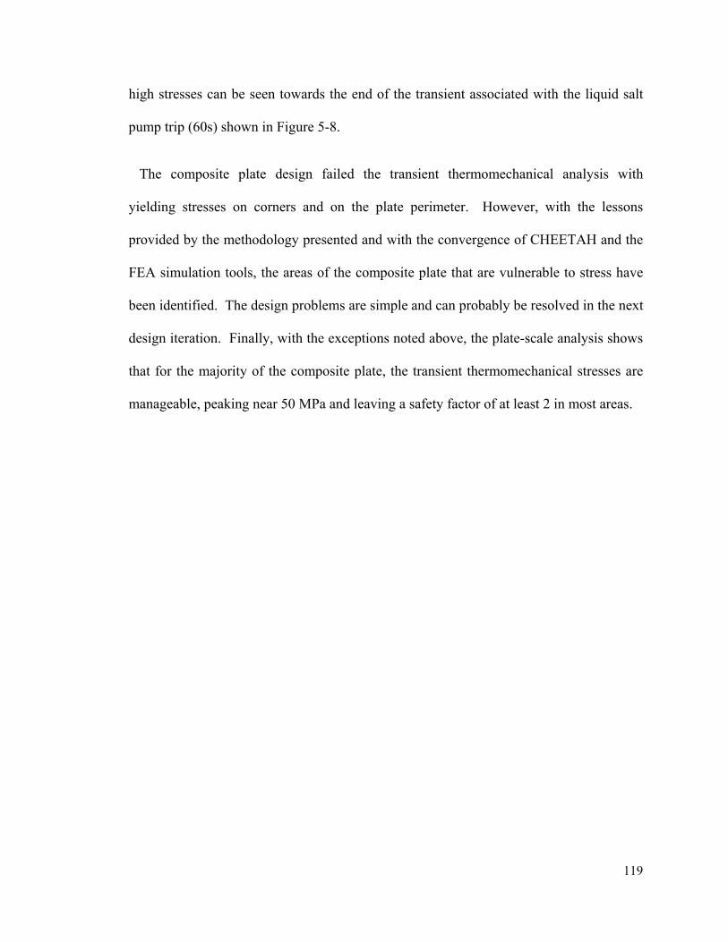
119
high stresses can be seen towards the end of the transient associated with the liquid salt
pump trip (60s) shown in Figure 5-8.
The composite plate design failed the transient thermomechanical analysis with
yielding stresses on corners and on the plate perimeter. However, with the lessons
provided by the methodology presented and with the convergence of CHEETAH and the
FEA simulation tools, the areas of the composite plate that are vulnerable to stress have
been identified. The design problems are simple and can probably be resolved in the next
design iteration. Finally, with the exceptions noted above, the plate-scale analysis shows
that for the majority of the composite plate, the transient thermomechanical stresses are
manageable, peaking near 50 MPa and leaving a safety factor of at least 2 in most areas.

120
5.6 Fin-scale Stress Analysis
Plotting the plate-scale principle stresses will show only the x or z components of the
stress distribution rather than the average or Von Mises stresses. With the principle
stresses on the plate-scale, the peak stresses in each unit cell region can be selected for
both the x and z directions. The peak principle stresses for each unit cell were found from
the plate-scale results and are listed in Table 5-2.
Local principle stresses on unit cells at each temperature state (MPa)
Unit Cells A B C D Steady-state (0s) x-dir 16.2 23.7 35.7 43.9 z-dir 14.8 14.8 14.8 14.8 LS 30 sec x-dir 25 70 35 20 z-dir 10 30 30 10 He 30 sec x-dir 10 10 15 70 z-dir 10 50 10 10 LS 60 sec x-dir 10 70 40 25 z-dir 10 20 20 5.5 He 60 sec x-dir 23 5 20 55 z-dir 20 60 20 20
Table 5-2: Local principle stresses on unit cells at each temperature state (MPa)
To recreate the plate-scale stresses on each unit cell a model of each unit cell is
imported to the FEA software (ANSYS). To replicate the pressure difference across the
composite plate, the fluid pressure for the helium (7MPa) is applied to its heat transfer
surface while 150 kPa is applied to the heat transfer surface corresponding to the liquid
salt surface area. Then, applying the corresponding principle stresses to the x and z faces
from Table 5-2 and constraining the opposite face in each direction, the plate-scale stress
state can be recreated on the unit cell. The fin-scale stresses were analyzed in ANSYS
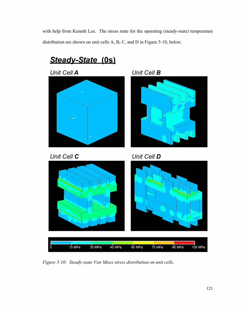
121
with help from Kennth Lee. The stress state for the operating (steady-state) temperature
distribution are shown on unit cells A, B, C, and D in Figure 5-10, below.
Figure 5-10: Steady-state Von Mises stress distribution on unit cells.

122
The stresses illustrated in Figure 5-10 show that the composite plate is sufficiently
robust to momentarily resist the operational steady-state stresses. Peak stresses occur in
the sharp corner regions as expected but even these leave an acceptable safety factor
when considering that only unit cells A and B will be close to peak temperatures. Here
again, it is the creep resistance that is lacking. Unit cells C and D show stresses
significantly above the 16 MPa maximum design stress (2 SF, or safety factor) for
Inconel Alloy 617. Like the composite plate, the inclusion of fillets in the unit cells
would likely reduce stresses significantly.

123
5.7 Stress Results from the Helium Pump Trip
The stress state corresponding to 30 seconds after the helium pump trip is obtained by
applying the pressure difference on each unit cell in addition to the stresses from Table 5-
2. The resulting stress state can be seen on unit cells A, B, C, and D in Figure 5-11,
below.
Figure 5-11: Transient Von Mises stress distribution on unit cells 30 seconds after the
helium pump trip.
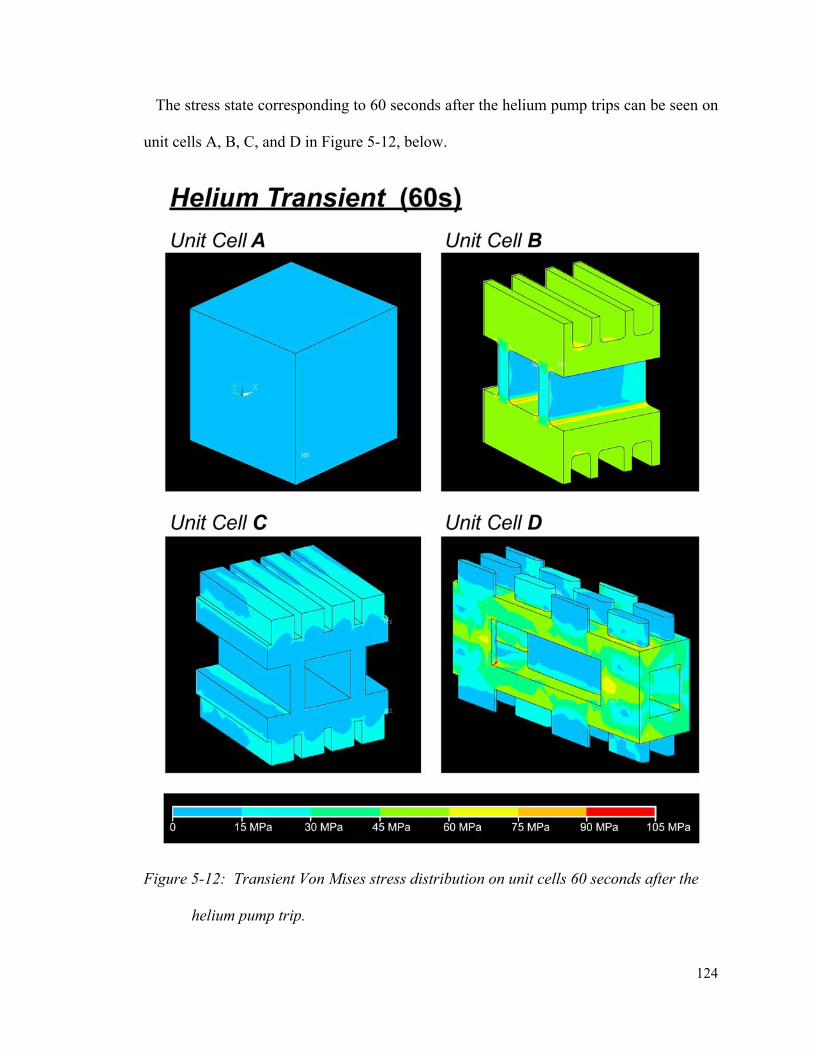
124
The stress state corresponding to 60 seconds after the helium pump trips can be seen on
unit cells A, B, C, and D in Figure 5-12, below.
Figure 5-12: Transient Von Mises stress distribution on unit cells 60 seconds after the
helium pump trip.
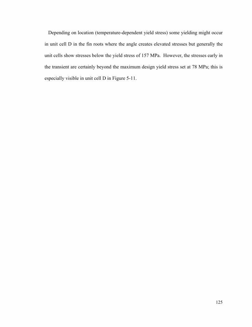
125
Depending on location (temperature-dependent yield stress) some yielding might occur
in unit cell D in the fin roots where the angle creates elevated stresses but generally the
unit cells show stresses below the yield stress of 157 MPa. However, the stresses early in
the transient are certainly beyond the maximum design yield stress set at 78 MPa; this is
especially visible in unit cell D in Figure 5-11.
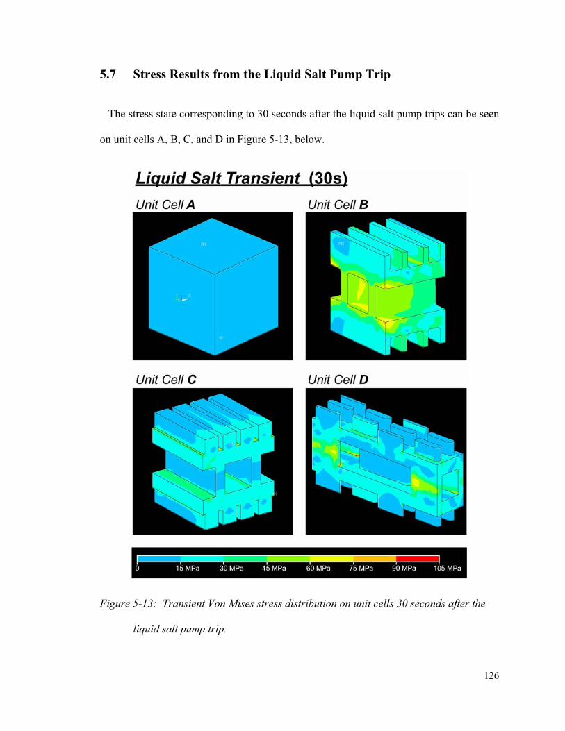
126
5.7 Stress Results from the Liquid Salt Pump Trip
The stress state corresponding to 30 seconds after the liquid salt pump trips can be seen
on unit cells A, B, C, and D in Figure 5-13, below.
Figure 5-13: Transient Von Mises stress distribution on unit cells 30 seconds after the
liquid salt pump trip.

127
The stress state corresponding to 60 seconds after the liquid salt pump trips can be seen
on unit cells A, B, C, and D in Figure 5-14, below.
Figure 5-14: Transient Von Mises stress distribution on unit cells 60 seconds after the
liquid salt pump trip.

128
The liquid salt pump trip shows thermomechanical stresses that are more moderate than
those associated with the helium pump trip. The stresses do not appear large enough to
cause yielding; however, the maximum design stress of 78 MPa (SF 2) is exceeded. By
including fillets in the fin roots the geometries in these unit cells can be made to resist the
transient thermomechanical stresses associated with a liquid salt pump trip.
129
Chapter 6
Conclusions and Recommendations
6.1 Recommendations Regarding Example Problem
From the mechanical results presented in the previous chapter it is clear that at peak
temperatures of 1200 K, Inconel Alloy 617 retains a formidable yield stress of 157 MPa.
The results provided by CHEETAH and ANSYS show that this is sufficient to resist the
very severe thermo-mechanical transient caused by the liquid salt and helium pump trips.
This is particularly notable since these pump failures are modeled as a 98% step down in
flow of one of the fluids which produces a deeply unbalanced counter-flow condition in
the IHX.
6.1.1 System Recommendations
One possibility to reduce the severity of thermal hydraulic transients associated with
pump failure or trip would be to include large flywheels on the centrifugal pump axels.
This would add rotational inertia to the system making the pump output ramp down more
gradually and thus reduce the shock associated with a more abrupt change in flow rate.
The size of the flywheels will depend on the vulnerability of the entire loop to flow and
thermal transients and will require detailed analysis to determine. CHEETAH can
130
contribute with the thermal hydraulic results associated with the compact heat exchangers
in the system.
Another idea to reduce the intensity of these types of flow transients involves
installing a pump trip relay that would automatically trip the counter-flow pump when
one pump trips. By tripping both pumps simultaneously the temperature transient on the
heat exchanger can be significantly reduced. Currently the trip of just one pump causes a
severe transient because the counter-flowing fluid continues to remove or deposit thermal
energy without adjusting to the conditions on the opposite side of the composite plate.
The simultaneous trip would help keep a thermal balance on the temperature distribution
while conduction effects more slowly take the system to thermal equilibrium.
Placing several shorter intermediate heat exchangers in series would reduce the
temperature change over any one heat exchanger significantly. The illustrative example
analyzed must endure a temperature change of 300°C from one end to the other; placing
three smaller heat exchangers in series could obtain the same total temperature drop but
with only a 100°C temperature change in each device. Lastly, the first heat exchanger
contacting the hot helium gas could have a specialized design, such as a bayonette or
shell and tube design to better cope with the creep stresses at high temperature while the
rest of the heat exchangers could be plate-type diffusion bonded heat exchangers like the
one presented in this illustrative example.

131
6.1.2 Hydraulic Recommendations
The selection of helium as a coolant in constant heat flux and high temperature
applications must be accompanied by careful thermal hydraulic analysis particularly
because the viscosity of helium gas rises with increasing temperatures [16]. This fact is
particularly important with regard to the formation and grown of hot spots in a high
temperature component cooled by helium. Hotter areas will increase local helium gas
coolant temperatures and viscosities, thereby decreasing coolant flow rates and creating
positive thermal feedback that leads to continuously increasing local temperatures. In the
illustrative example analyzed the intermediate heat exchanger used high pressure helium
not as the coolant but rather as the hot fluid. However, on the opposite side of that hot
loop the high pressure helium is the coolant in the modular helium reactor (MHR). This
is a case where careful consideration of temperature dependant fluid properties is
paramount.
Another complication from helium concerns its low volumetric heat capacity relative
to the liquid salt. This entails that the helium be used at high pressure to increase its
density and it means that large flow rates are required in the helium side of the composite
plate. High flow rates demand relatively high pumping power be expended on the helium
flow compared to that in the liquid salt flow. The low volumetric heat capacity of helium
also necessitates a large temperature rise in the helium compared to that of the liquid salt.
The large temperature and pressure difference between fluids is responsible for the large
stresses in the IHX which must be resisted at high temperature. Optimally, a high
temperature heat exchanger would operate between fluids operating with a low pressure

132
difference between them and with a more moderate temperature change between inlet and
outlet.
6.1.3 Mechanical Recommendations
The mechanical stress analysis in Chapter 5 highlights an important trend in the
vulnerability of the composite plate. The stress plots (Figures 5-5, 5-6, and 5-7) resulting
from the thermal hydraulic analysis using CHEETAH demonstrate that the there are
fundamentally two phenomena that threaten the integrity of the composite plate; these are
transient yielding and operational creep deformation. In both cases stresses concentrate
on the perimeter of the composite plate but the reasons for stress intensity are different.
Regarding transient yielding stress, the CHEETAH code shows that large temperature
gradients are associated with the thicker sections in the composite plate. These are
sections that have a high thermal inertia (100% solid phase fraction) and only exchange
heat by conduction, which means that they take longer to equilibrate than the sections in
direct contact with the heat transfer fluids which can exchange heat via both conduction
and convection. Thick walls dominate the perimeter of the composite plate, reducing the
thickness of this perimeter will likely solve the transient yielding stress problem with this
heat exchanger. This hypothesis can be tested by subjecting a redesigned composite plate
to the same thermal hydraulic analysis with CHEETAH as the one performed on the
composite plate geometry presented in this study. A redesigned plate that addresses these
and other issues can be seen below in Figure 6-1.
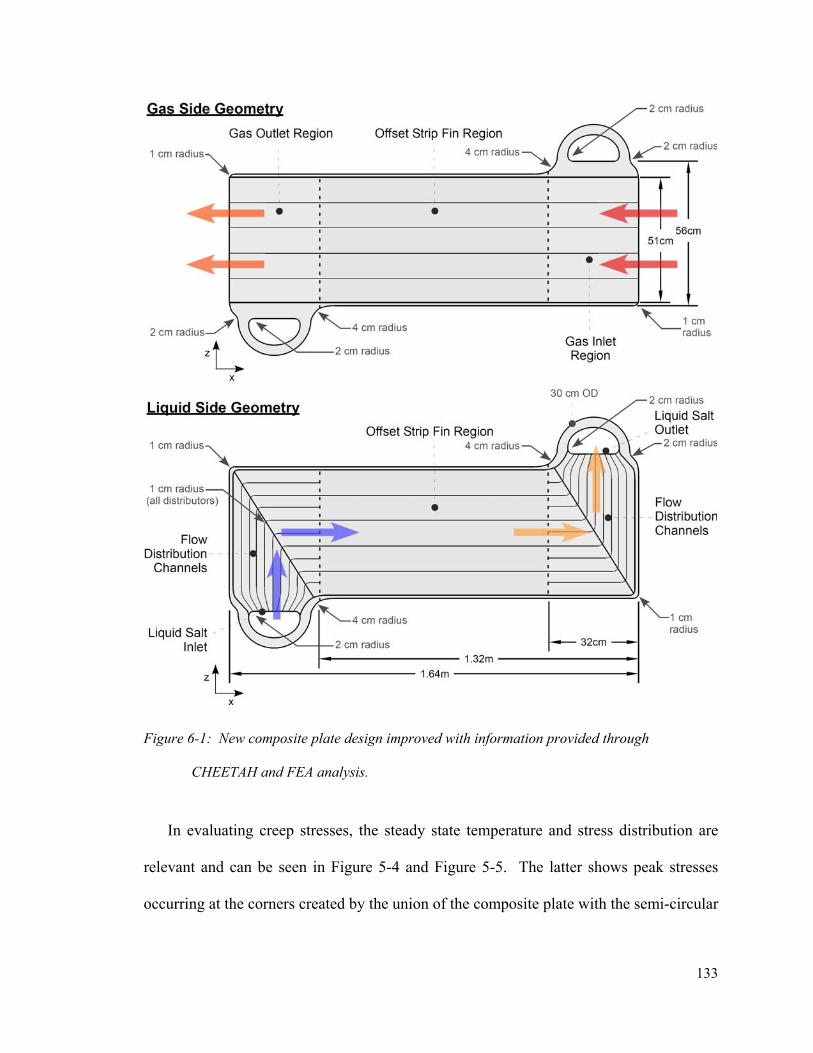
133
Figure 6-1: New composite plate design improved with information provided through
CHEETAH and FEA analysis.
In evaluating creep stresses, the steady state temperature and stress distribution are
relevant and can be seen in Figure 5-4 and Figure 5-5. The latter shows peak stresses
occurring at the corners created by the union of the composite plate with the semi-circular
134
liquid salt manifolds as well as in the areas where the plate thickness is significantly
reduced. These stresses can be avoided with large fillets in the corners between pipe
manifolds and rectangular plates. Furthermore, the reduction in plate thickness between
the liquid slat manifold and the side of the composite plate must be executed more
gradually culminating in thinner sections as can be seen in the redesigned composite plate
shown in Figure 6-1, above.
The steady state or operational temperature gradients in the composite plate that are
relevant for the creep analysis are quite mild. Still, flow maldistribution in the OSF
region creates some temperature gradients large enough to create thermo-mechanical
stresses above the design limit for creep which is set at 16 MPa. In order to avoid this
mode of failure, the OSF section could be divided into six flow zones rather than the
current five. This would reduce the difference in velocities from the inside to outside
corner of each flow zone that can be seen as ridges in Figure 3-4 and Figure 3-13.
Additionally, the OSF geometry must be made more robust. This can be done by
significantly reducing the gas and liquid fin heights and by including large fillets at the
base of fins and in channels. Shortening fins will increase the number of plates in an IHX
assembly while modifications to include large fillets will have the side benefit of
reducing flow friction in the OSF region to the detriment of heat transfer.
Yet another option is to avoid the creep problems all together by using a material with
a larger yield stress at the peak temperatures of 1200 K (927°C). Ceramics would offer
the creep resistance but may be more vulnerable to thermo-mechanical transients.
135
Research at UC Berkeley has explored the possibility of making a compact IHX out a
silicon-carbide based ceramic material via a molding process [26].
6.2 Conclusions
The previous chapters have covered a multi-scale thermal, hydraulic, and mechanical
analysis of a high temperature compact intermediate heat exchanger. This work
characterized the heat exchanger’s internal geometry by analyzing a representative
composite plate which includes geometry from both gas and liquid plates. This
composite plate was further parsed into several zones containing unique geometrical
configurations including repetitive small scale features. Unit cells containing these
features which are also representative of the zones from which they were obtained are
then analyzed and their effective thermal, hydraulic, and mechanical properties are
derived. A separate model is build based on these effective or volume averaged
properties; this model is analyzed using an FVA code developed for this purpose called
Compact Heat Exchanger Explicit and Hydraulics (CHEETAH) code.
The model analyzed in CHEETAH is designed to capture the phenomena created by
the small features in the original heat exchanger without forcing discretization at this
small scale. The steady state and transient thermal hydraulic response of this system was
analyzed in CHEETAH using modest computational resources. These results lead to
thermal hydraulic optimization of the heat exchanger and also to a multi-scale mechanical
136
analysis in ANSYS that identifies the more vulnerable areas of the design so that they can
be improved.
This method and its implementation in CHEETAH enable the transient thermal
hydraulic computation of a complex system containing descriptive dimensions too small
to discretize individually. The CHEETAH code bridges multiple scales to effectively
analyze at the component scale (composite plate).
This method does have its limitations, however. Yet more work is required to
improve usability and to facilitate the adaptability of the code to different geometries.
Also, by performing a volume average of fin-scale effects the variation in performance at
that is dependent on the correlation used to define volume averaged behavior rather than
on first principles. Furthermore, discontinuities in properties occur at the boundaries
between zones with effective properties, and while the distortions in this case are small, if
the analysis were searching for subtle effects, the distortions could dominate. Finally,
just as the ability to discretize at a larger scale enables faster and transient analyses it also
means limits the resolution of the thermal hydraulic data obtained.
In conclusion, the successful application of this code to the example problem shows
the potential of carefully undertaken volume averaging. The CHEETAH code is a tool
that together with FEA software can help designers and researchers analyze and optimize
the thermal, hydraulic, and mechanical performance of a plate-type compact heat
exchanger. The code also readily provides insightful performance data regarding the
effects of temperature dependent fluid properties on flow distribution in a high
temperature heat exchanger. Lastly, the results from CHEETAH can be used to provide

137
boundary conditions for an analysis at a smaller scale. Subsequent analyses at a smaller
scale can be executed using CFD or by adapting the algorithms used in CHEETAH to
detailed geometry at the new scale with appropriate local volume averaging.

138
References
[1] Urquiza-Fernández E., Peterson P. F. and R. Greif. “Multi-Scale Thermal Analysis for Compact Plate-Type Heat Exchangers.” American Institute of Chemical Engineering Annual Meeting, Salt Lake City, UT, November 4-9, 2007.
[2] Huang W., Zhao H. and P. F. Peterson. “Multi-scale Stress Analysis for Compact Plate Heat Exchangers.” 2006 International Congress on Advances in Nuclear Power Plants (ICAPP 2006), Reno, NV, June 4-8, 2006.
[3] Dewson S. J. and B. Thonon. The Development of High Efficiency Heat Exchangers for Helium Gas Cooled Reactors (Paper No. 3213). 2003 International Congress on Advances in Nuclear Power Plants (ICAPP 2003).
[4] Williams D. F. et al. Assessment of Candidate Molten Salt Coolants for the Advanced High-Temperature Reactor (AHTR); ORNL/TM-2006/12; Oak Ridge National Laboratory, Oak Ridge, TN, March 2006.
[5] Peaceman, D. W., Fundamentals of Numerical Reservoir Simulation. Elsevier, 1977. ISBN 0444415785, 9780444415783
[6] Domenico, P. A. and F. W. Schwartz, Physical and Chemical Hydrogeology. University of Michigan: Wiley & Sons, 1990
[7] Ponyavin, V. et al., “The Flow Calculation in the High Temperatured Heat Exchanger with the Manufactring geometrical Effects.” Proceedings of the 2005 Summer Heat Transfer Conference, San Francisco, CA, USA.
[8] Hu, S. and K. E. Herold. “Prandtl number effect on offset fin heat exchanger performance: predictive model for heat transfer and pressure drop.” Int. J. Heat Mass Transfer 38, No. 6 (1995): 1043-1051.
139
[9] Kays W. M. and A. L. London. Compact Heat Exchangers. 3rd ed., New York, NY: McGraw-Hill, 1984.
[10] Manglik R. M. and A. E. Bergles. “Heat Transfer and Pressure Drop Correlations for the Rectangular Offset Strip Fin Compact Heat Exchanger.” Experimental Thermal and Fluid Science 10 (1995): 171-180.
[11] Fox R. W. and A. T. McDonald. Introduction to Fluid Mechanics. 3rd ed., Wiley & Sons, 1985.
[12] Kays, W. M., “Compact Heat Exchangers,” AGARD Lecture Ser. No. 57 on Heat Exchangers, AGARD-LS-57-72, NATO, Paris, 1972.
[13] Sparrow E.M., B.R. Baliga and S.V. Patankar, “Heat transfer and fluid flow analysis of interrupted-wall channels with application to heat exchangers,” J. Heat Transfer 22, 1613-1625 (1977).
[14] Kelkar K.M. and S.V. Patankar, “Numerical prediction of heat transfer and fluids flow sin rectangular offset-fin arrays,” Numerical Heat Transfer A 15, 149-164 (1989).
[15] Anderson D. A., J.C. Tannehill, and R. H. Pletcher. Computational Fluid Mechanics and Heat Transfer. New York, NY: McGraw-Hill, 1984.
[16] National Institute for Standards and Technology, NIST. www.nist.gov.
[17] Mills A. F. Heat and Mass Transfer. Concord, MA: Irwin, 1995.
[18] Incropera F. and D. P. DeWitt. Fundamentals of Heat and Mass Transfer. 5th ed., Wiley & Sons, 2002.
[19] Çengel Y. A. and R. H. Turner. Thermal-Fluid Sciences. New York, NY: McGraw-Hill, 2001.
[20] Patankar S.V. Numerical Heat Transfer and Fluid Flow. New York, NY: McGraw-Hill, 1980.
140
[21] Yin J. and M. K. Jensen. “Analytic Model for Transient Heat Exchanger Response.” Int. J. Heat Mass Transfer 46 (2003): 3255-3264.
[22] F.E. Romie, “Transient response of the counterflow heat exchanger,” J. Heat Transfer 106 (3) (1984) 620–626.
[23] W. Roetzel, Y. Xuan, “Transient response of parallel and counterflow heat exchangers,” J. Heat Transfer 114 (2) (1992) 510–512.
[24] Boresi, A.P. and R.J. Schmidt. Advanced Mechanics of Materials. Wiley & Sons, 2003.
[25] Haynes International, Inc., “Heat-resistant alloy-at-a-glance: Haynes 617 alloy.” http://www.haynesintl.com.
[26] Peterson P. F., Zhao H., Niu F. and W. Huang, Schmidt J. and J. Schulte-Fischedick. “Development of C-SiC ceramic compact plate heat exchangers for high temperature heat transfer applications.” American Institute of Chemical Engineering Annual Meeting, San Francisco, CA, November 12-16, 2006.

141
Appendix A
Intermediate Heat Exchanger Sizing Calculations Mathcad spreadsheet design by Dr. Hai Hua Zhao
Modified by Eugenio Urquiza
Flow channel geometries:
Unit Cell D - Offset strip fin region of the IHX
effective fin thickness coefficient: Cfin 0.5:=
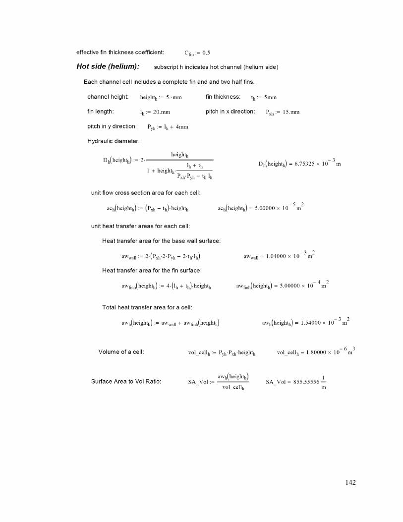
142
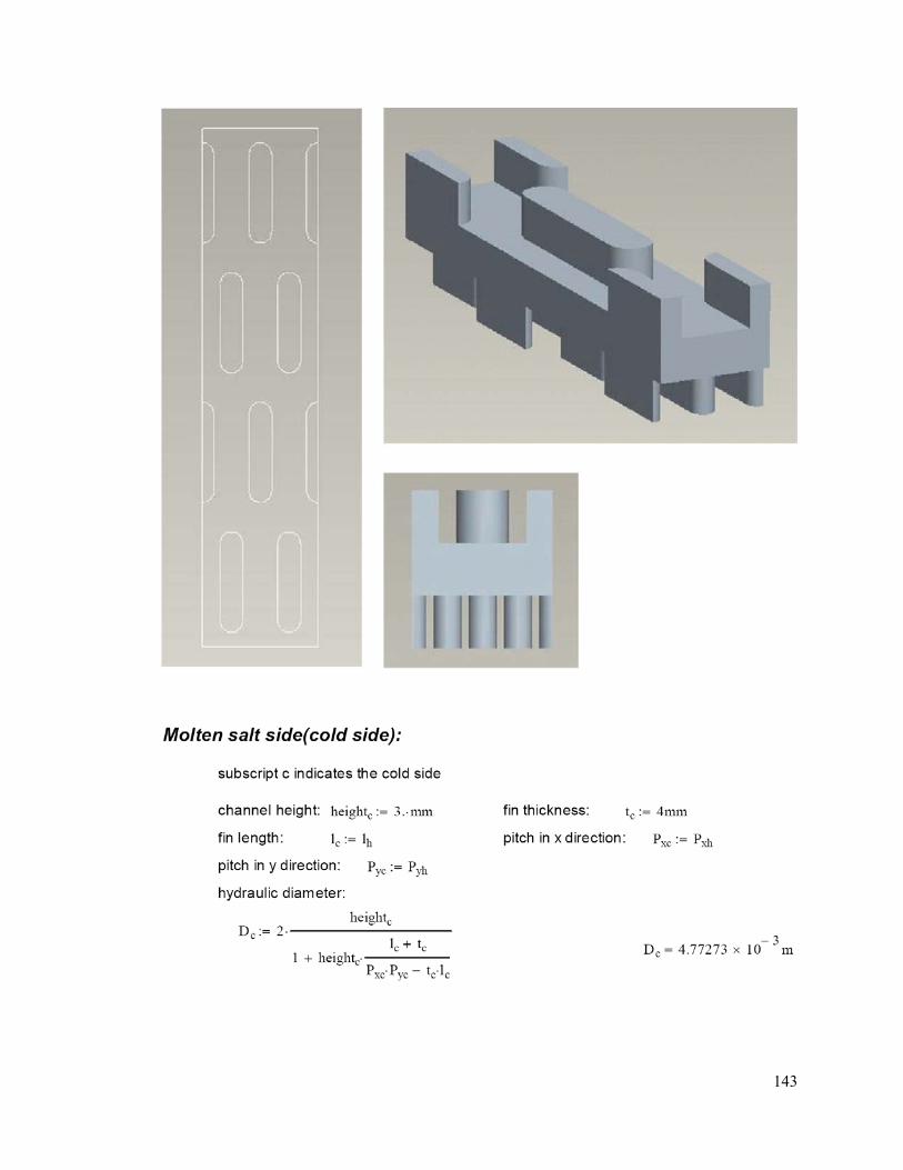
143
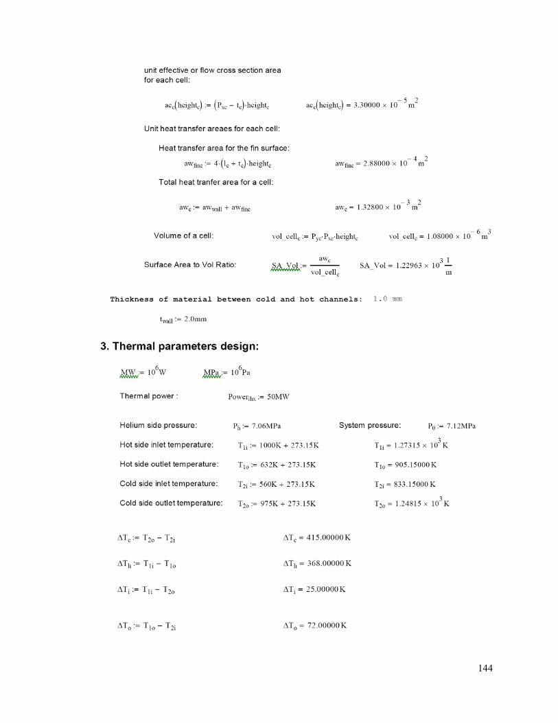
144

145
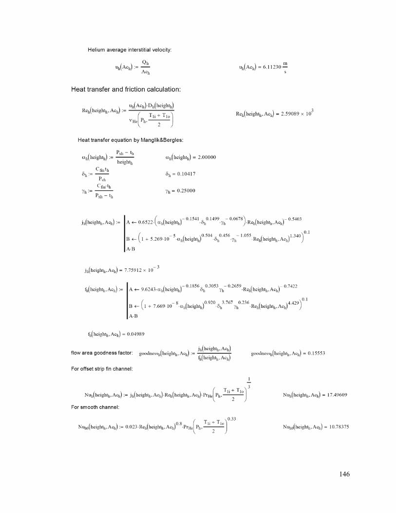
146
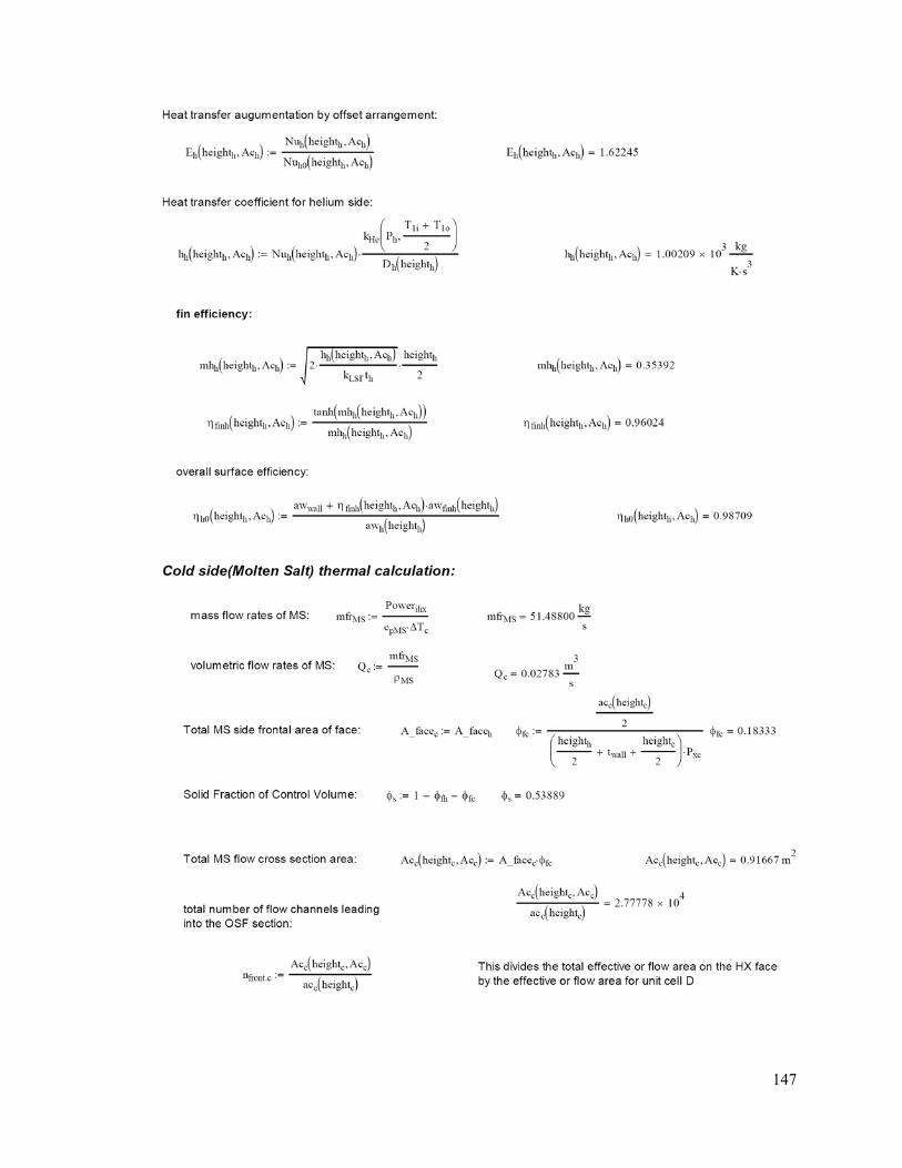
147
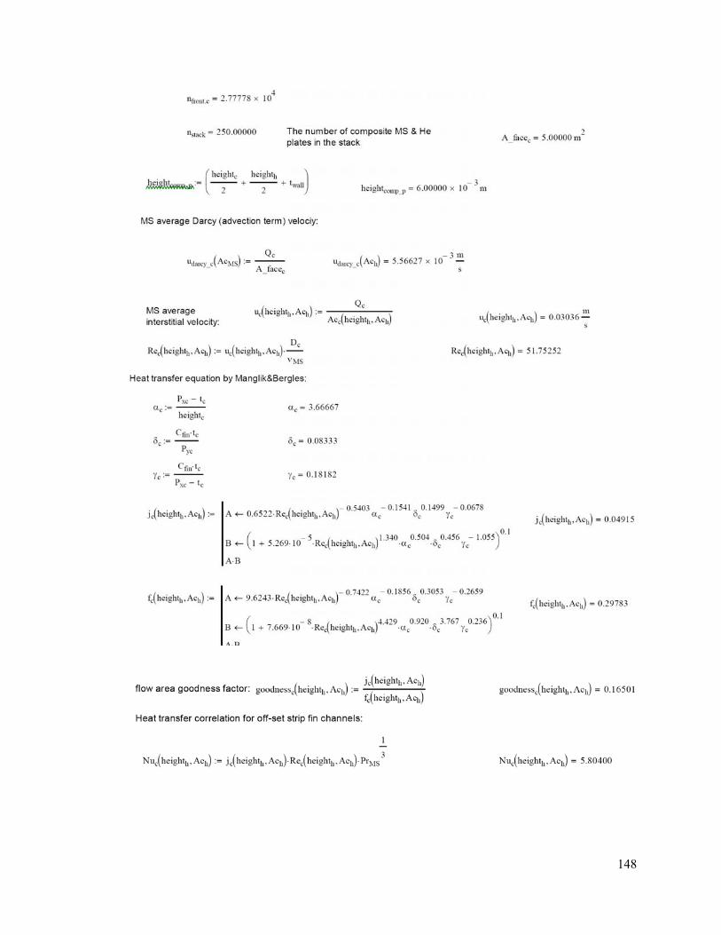
148
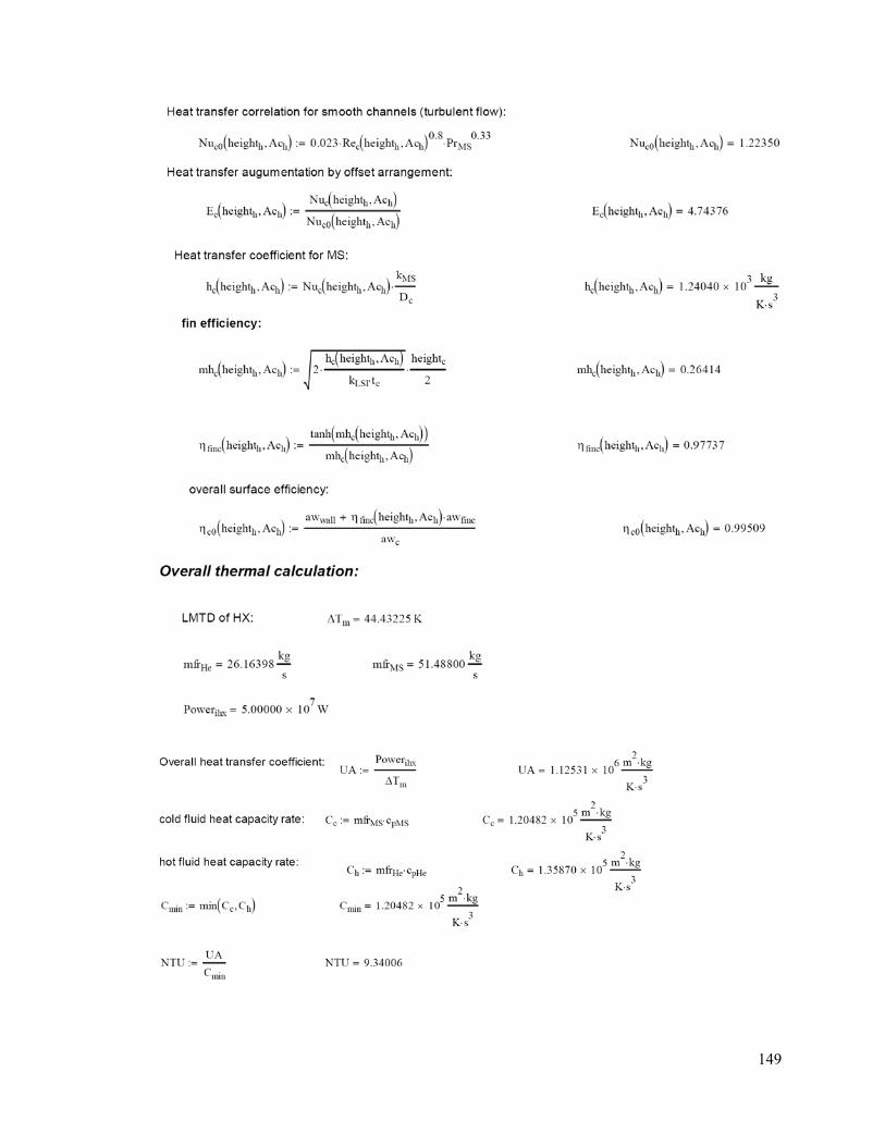
149
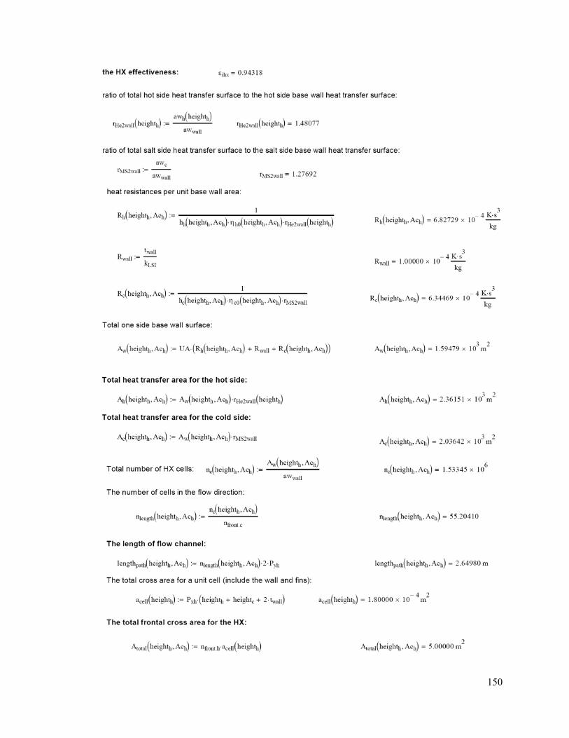
150
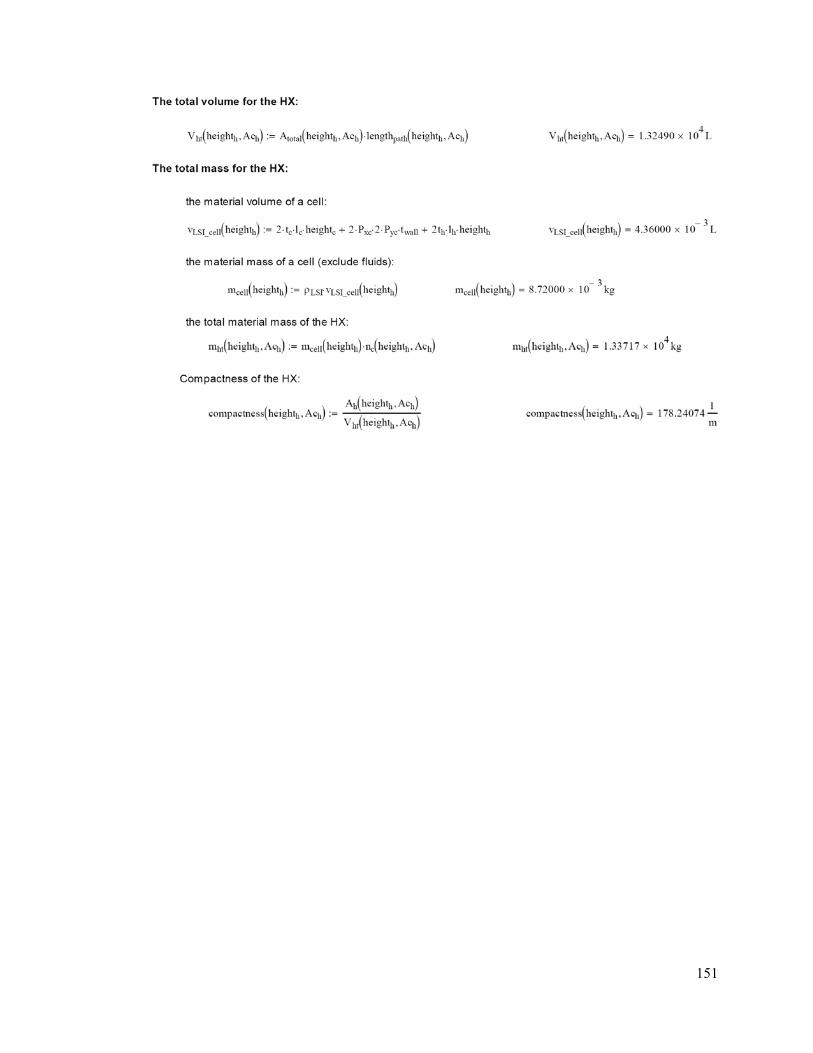
151

152
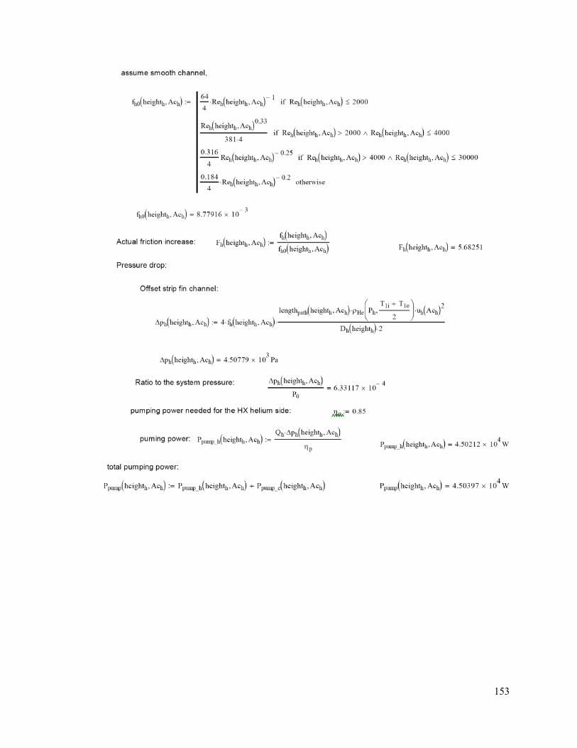
153

154
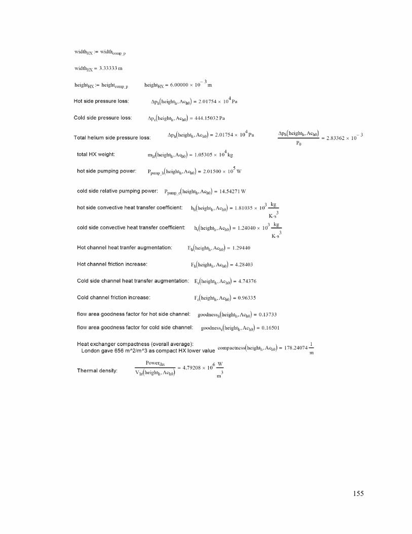
155
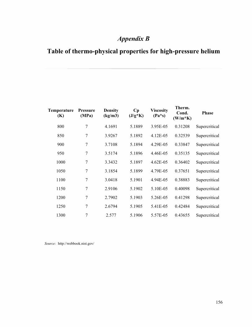
156
Appendix B
Table of thermo-physical properties for high-pressure helium
Source: http://webbook.nist.gov/
Temperature (K)
Pressure (MPa)
Density (kg/m3)
Cp (J/g*K)
Viscosity (Pa*s)
Therm. Cond.
(W/m*K) Phase
800 7 4.1691 5.1889 3.95E-05 0.31208 Supercritical
850 7 3.9267 5.1892 4.12E-05 0.32539 Supercritical
900 7 3.7108 5.1894 4.29E-05 0.33847 Supercritical
950 7 3.5174 5.1896 4.46E-05 0.35135 Supercritical
1000 7 3.3432 5.1897 4.62E-05 0.36402 Supercritical
1050 7 3.1854 5.1899 4.79E-05 0.37651 Supercritical
1100 7 3.0418 5.1901 4.94E-05 0.38883 Supercritical
1150 7 2.9106 5.1902 5.10E-05 0.40098 Supercritical
1200 7 2.7902 5.1903 5.26E-05 0.41298 Supercritical
1250 7 2.6794 5.1905 5.41E-05 0.42484 Supercritical
1300 7 2.577 5.1906 5.57E-05 0.43655 Supercritical
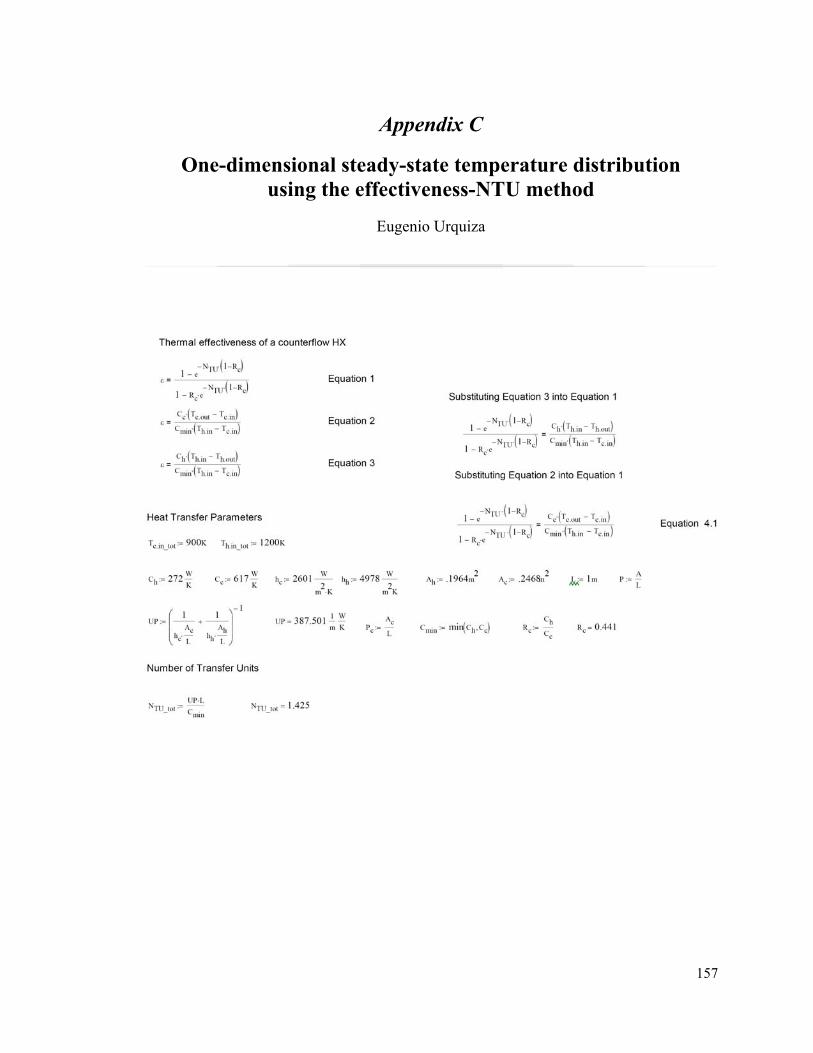
157
Appendix C
One-dimensional steady-state temperature distribution using the effectiveness-NTU method
Eugenio Urquiza

158
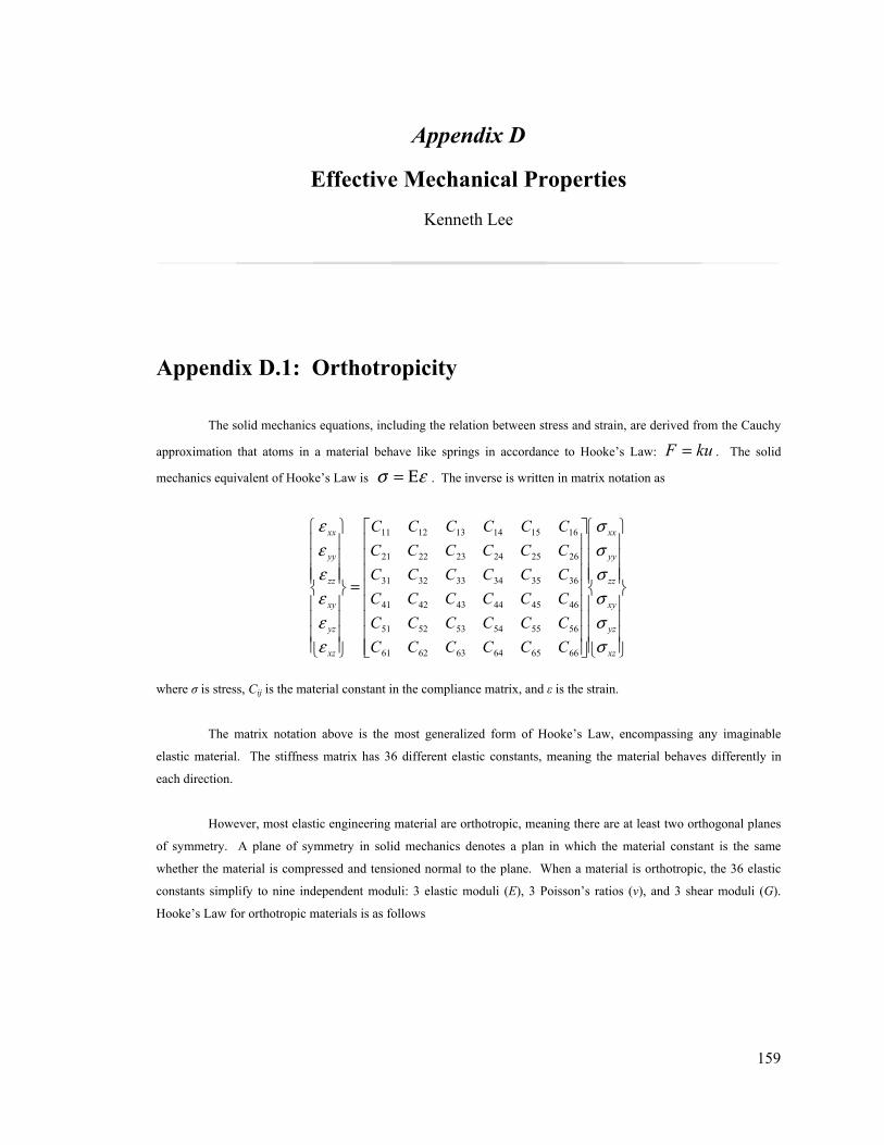
159
Appendix D
Effective Mechanical Properties Kenneth Lee
Appendix D.1: Orthotropicity The solid mechanics equations, including the relation between stress and strain, are derived from the Cauchy
approximation that atoms in a material behave like springs in accordance to Hooke’s Law: kuF = . The solid
mechanics equivalent of Hooke’s Law is εσ Ε= . The inverse is written in matrix notation as
⎪⎪⎪⎪
⎭
⎪⎪⎪⎪
⎬
⎫
⎪⎪⎪⎪
⎩
⎪⎪⎪⎪
⎨
⎧
⎥⎥⎥⎥⎥⎥⎥⎥
⎦
⎤
⎢⎢⎢⎢⎢⎢⎢⎢
⎣
⎡
=
⎪⎪⎪⎪
⎭
⎪⎪⎪⎪
⎬
⎫
⎪⎪⎪⎪
⎩
⎪⎪⎪⎪
⎨
⎧
xz
yz
xy
zz
yy
xx
xz
yz
xy
zz
yy
xx
CCCCCCCCCCCCCCCCCCCCCCCCCCCCCCCCCCCC
σσσσσσ
εεεεεε
666564636261
565554535251
464544434241
363534333231
262524232221
161514131211
where σ is stress, Cij is the material constant in the compliance matrix, and ε is the strain.
The matrix notation above is the most generalized form of Hooke’s Law, encompassing any imaginable
elastic material. The stiffness matrix has 36 different elastic constants, meaning the material behaves differently in
each direction.
However, most elastic engineering material are orthotropic, meaning there are at least two orthogonal planes
of symmetry. A plane of symmetry in solid mechanics denotes a plan in which the material constant is the same
whether the material is compressed and tensioned normal to the plane. When a material is orthotropic, the 36 elastic
constants simplify to nine independent moduli: 3 elastic moduli (E), 3 Poisson’s ratios (ν), and 3 shear moduli (G).
Hooke’s Law for orthotropic materials is as follows
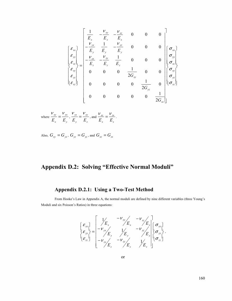
160
⎪⎪⎪⎪
⎭
⎪⎪⎪⎪
⎬
⎫
⎪⎪⎪⎪
⎩
⎪⎪⎪⎪
⎨
⎧
⎥⎥⎥⎥⎥⎥⎥⎥⎥⎥⎥⎥⎥⎥⎥⎥
⎦
⎤
⎢⎢⎢⎢⎢⎢⎢⎢⎢⎢⎢⎢⎢⎢⎢⎢
⎣
⎡
−−
−−
−−
=
⎪⎪⎪⎪
⎭
⎪⎪⎪⎪
⎬
⎫
⎪⎪⎪⎪
⎩
⎪⎪⎪⎪
⎨
⎧
xz
yz
xy
zz
yy
xx
xz
yz
xy
zz
zy
z
zx
y
yz
yy
yx
x
xz
x
xy
x
xz
yz
xy
zz
yy
xx
G
G
G
EEE
EEE
EEE
σσσσσσ
νν
νν
νν
εεεεεε
2100000
02
10000
002
1000
0001
0001
0001
where y
yx
x
xy
EEνν
= , z
zy
y
yz
EEνν
= , and z
zx
x
xz
EEνν
= .
Also, yxxy GG = , yzyz GG = , and zxxz GG =
Appendix D.2: Solving “Effective Normal Moduli”
Appendix D.2.1: Using a Two-Test Method From Hooke’s Law in Appendix A, the normal moduli are defined by nine different variables (three Young’s
Moduli and six Poisson’s Ratios) in three equations:
⎪⎭
⎪⎬
⎫
⎪⎩
⎪⎨
⎧
⎥⎥⎥⎥⎥⎥
⎦
⎤
⎢⎢⎢⎢⎢⎢
⎣
⎡
−−
−−
−−
=⎪⎭
⎪⎬
⎫
⎪⎩
⎪⎨
⎧
zz
yy
xx
zz
zy
z
zx
y
yz
yy
yx
x
xz
x
xy
x
zz
yy
xx
EEE
EEE
EEE
σσσ
νν
νν
νν
εεε
1
1
1
.
or
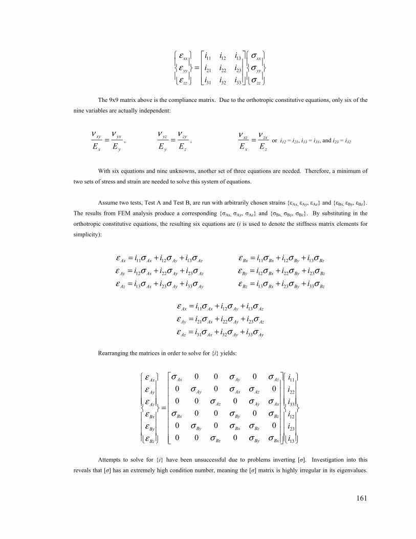
161
11 12 13
21 22 23
31 32 33
xx xx
yy yy
zz zz
i i ii i ii i i
ε σε σε σ
⎧ ⎫ ⎡ ⎤ ⎧ ⎫⎪ ⎪ ⎪ ⎪⎢ ⎥=⎨ ⎬ ⎨ ⎬⎢ ⎥⎪ ⎪ ⎪ ⎪⎢ ⎥⎩ ⎭ ⎣ ⎦ ⎩ ⎭
The 9x9 matrix above is the compliance matrix. Due to the orthotropic constitutive equations, only six of the
nine variables are actually independent:
y
yx
x
xy
EEνν
= , z
zy
y
yz
EEνν
= , z
zx
x
xz
EEνν
= or i12 = i21, i13 = i31, and i23 = i32
With six equations and nine unknowns, another set of three equations are needed. Therefore, a minimum of
two sets of stress and strain are needed to solve this system of equations.
Assume two tests, Test A and Test B, are run with arbitrarily chosen strains {εAx, εAy, εAz} and {εBx, εBy, εBz}.
The results from FEM analysis produce a corresponding {σAx, σAy, σAz} and {σBx, σBy, σBz}. By substituting in the
orthotropic constitutive equations, the resulting six equations are (i is used to denote the stiffness matrix elements for
simplicity):
AzAyAxAx iii σσσε 131211 ++= BzByBxBx iii σσσε 131211 ++= AzAyAxAy iii σσσε 232212 ++= BzByBxBy iii σσσε 232212 ++= AyAyAxAz iii σσσε 332313 ++= BzByBxBz iii σσσε 332313 ++=
AzAyAxAx iii σσσε 131211 ++=
21 22 23Ay Ax Ay Azi i iε σ σ σ= + + 31 32 33Az Ax Ay Ayi i iε σ σ σ= + +
Rearranging the matrices in order to solve for {i} yields:
⎪⎪⎪⎪
⎭
⎪⎪⎪⎪
⎬
⎫
⎪⎪⎪⎪
⎩
⎪⎪⎪⎪
⎨
⎧
⎥⎥⎥⎥⎥⎥⎥⎥
⎦
⎤
⎢⎢⎢⎢⎢⎢⎢⎢
⎣
⎡
=
⎪⎪⎪⎪
⎭
⎪⎪⎪⎪
⎬
⎫
⎪⎪⎪⎪
⎩
⎪⎪⎪⎪
⎨
⎧
13
23
12
33
22
11
000000
000000
000000
iiiiii
BxByBz
BzBxBy
BzByBx
AxAyAz
AzAxAy
AzAyAx
Bz
By
Bx
Az
Ay
Ax
σσσσσσ
σσσσσσ
σσσσσσ
εεεεεε
Attempts to solve for {i} have been unsuccessful due to problems inverting [σ]. Investigation into this
reveals that [σ] has an extremely high condition number, meaning the [σ] matrix is highly irregular in its eigenvalues.

162
Matrices with high condition numbers are relatively more difficult to manage in matrix algebra. Conveniently, a three-
test method involves more manageable matrices.
Appendix D.3: Using a Three-Test Method
Assume three tests, Test A, Test B, and Test C, are run with arbitrarily chosen strains {εAx, εAy, εAz}, {εBx, εBy,
εBz}, and {εCx, εCy, εCz}. The results from FEM analysis produce a corresponding {σAx, σAy, σAz}, {σBx, σBy, σBz}, and
{σCx, σCy, σCz}. Neglecting the orthotropic constitutive equations, the resulting nine equations are (i is again used to
denote the stiffness matrix elements for simplicity):
AzAyAxAx iii σσσε 131211 ++= BzByBxBx iii σσσε 131211 ++= CzCyCxCx iii σσσε 131211 ++=
AzAyAxAy iii σσσε 232212 ++= BzByBxBy iii σσσε 232212 ++= CzCyCxCx iii σσσε 131211 ++=
AyAyAxAz iii σσσε 332313 ++= BzByBxBz iii σσσε 332313 ++= CzCyCxCx iii σσσε 131211 ++=
With three sets of data, different matrix equations can be created which could not be done with only two sets:
⎪⎭
⎪⎬
⎫
⎪⎩
⎪⎨
⎧
⎥⎥⎥
⎦
⎤
⎢⎢⎢
⎣
⎡
=⎪⎭
⎪⎬
⎫
⎪⎩
⎪⎨
⎧
13
12
11
iii
CzCyCx
BzByBx
AzAyAx
Cx
Bx
Ax
σσσσσσσσσ
εεε
⎪⎭
⎪⎬
⎫
⎪⎩
⎪⎨
⎧
⎥⎥⎥
⎦
⎤
⎢⎢⎢
⎣
⎡
=⎪⎭
⎪⎬
⎫
⎪⎩
⎪⎨
⎧
23
22
21
iii
CzCyCx
BzByBx
AzAyAx
Cy
By
Ay
σσσσσσσσσ
εεε
⎪⎭
⎪⎬
⎫
⎪⎩
⎪⎨
⎧
⎥⎥⎥
⎦
⎤
⎢⎢⎢
⎣
⎡
=⎪⎭
⎪⎬
⎫
⎪⎩
⎪⎨
⎧
33
32
31
iii
CzCyCx
BzByBx
AzAyAx
Cz
Bz
Az
σσσσσσσσσ
εεε
In all three cases, the [σ] is an easy and manageable 3x3 matrix. These matrices can be easily solved for the
three sets of {i}. Since each iij corresponds to a term in the stiffness matrix, the individual terms for Young’s Modulus
and Poisson’s Ratios are solved. A secondary confirmation can be performed to check if the constitutive equations: i12
= i21, i13 = i31, and i23 = i32 still holds. For all unit cells, these equations still held.
Madenci, E. and I. Guven. The Finite Element Method and Applications in Engineering Using ANSYS®. New York:
Springer Science+Business Media, Inc., 2006.
Boresi, A.P. and R.J. Schmidt. Advanced Mechanics of Materials. USA: John Wiley & Sons, Inc., 2003.

163
Appendix D.4: Effective Thermal Conductivity
Procedure: In calculating the “effective thermal moduli,” the unit cell of each region is assumed to have thermal
conductivities in three orthogonal directions x, y, and z. The conduction rate equation (or Fourier’s Law) can be written
on in matrix form as the following:
⎪⎪⎪
⎭
⎪⎪⎪
⎬
⎫
⎪⎪⎪
⎩
⎪⎪⎪
⎨
⎧
Δ
Δ
Δ
⎥⎥⎥
⎦
⎤
⎢⎢⎢
⎣
⎡−=
⎪⎪⎪
⎭
⎪⎪⎪
⎬
⎫
⎪⎪⎪
⎩
⎪⎪⎪
⎨
⎧
z
z
y
y
x
x
z
y
x
z
z
y
y
x
x
lT
lT
lT
kk
k
Aq
Aq
Aq
000000
The thermal conductivities are defined by four unknowns in three equations. To solve for the “effective
thermal moduli” of each unit cell, the geometry, temperature difference, and corresponding heat flux must be known.
FEM analysis is used to determine the corresponding heat flux for a given temperature difference.
Given any unit cell, a known temperature difference (arbitrarily chosen at 100K) is applied to one set of
opposing Cartesian faces. The remaining faces are kept insulated. The resulting heat on the temperature-induced faces
can be divided the total unit cell face area in order to get the corresponding heat flux. The heat flux is divided by the
temperature per unit length to solve for the heat conductivity in a certain Cartesian direction.
Alloy 617 is the material used to model the IHX unit cells. The isotropic heat conductivity at 800ºC is set at
25.5 W*m/K (High Temp Metals www.hightempmetals.com).
Findings: Same lengths of each unit cell and corresponding effective areas.
Chosen temperature difference: 100K (1100K-1000K)
Thermal Conductivities Heat transferred calculated from ANSYS [W]
x-direction y-direction z-direction
Unit Cell A 5.181600 5.181600 5.181600
Unit Cell B 1.347378 0.8270602 0.4800920
Unit Cell C 40.49833 61.18080 33.01654
Unit Cell D 156.6633 9.062221 29.30785
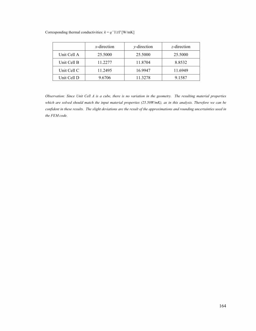
164
Corresponding thermal conductivities: k = q’’l/ΔT [W/mK]
x-direction y-direction z-direction
Unit Cell A 25.5000 25.5000 25.5000
Unit Cell B 11.2277 11.8704 8.8532
Unit Cell C 11.2495 16.9947 11.6949
Unit Cell D 9.6706 11.3278 9.1587
Observation: Since Unit Cell A is a cube, there is no variation in the geometry. The resulting material properties
which are solved should match the input material properties (25.50W/mK), as in this analysis. Therefore we can be
confident in these results. The slight deviations are the result of the approximations and rounding uncertainties used in
the FEM code.


