
Trading the Bond-CDS Basis - The Role of Credit Risk and
Liquidity
Monika Trapp∗
ABSTRACT
We analyze trading opportunities that arise from differences between the bond and the
CDS market. By simultaneously entering a position in a CDS contract and the underlying
bond, traders can build a default-risk free position that allows them to repeatedly earn the
difference between the bond asset swap spread and the CDS, known as the basis. We show
that the basis size is closely related to measures of company-specific credit risk and liquidity,
and to market conditions. In analyzing the aggregate profits of these basis trading strategies,
we document that dissolving a position leads to significant profit variations, but that attractive
risk-return characteristics still apply. The aggregate profits depend on the credit risk, liquidity,
and market measures even more strongly than the basis itself, and we show which conditions
make long and short basis trades more profitable. Finally, we document the impact of the
financial crisis on the profits of long and short basis trades, and show that the formerly more
profitable long basis trades experienced more drastic profit decreases than short basis trades.
JEL classification: C31, C32, G12, G13, G14, G32
Keywords: bond asset swap spreads, CDS premia, basis trading profits, credit risk, liquidity,
fixed-effects, vector error correction model
∗Department of Finance, University of Cologne, and Centre for Financial Research, D-50923 Cologne, e:
[email protected], t:++49 221 470 6966. Financial support from the Fritz Thyssen foundation is gratefully
acknowledged.

I. Introduction
The purpose of this paper is to explore the relationship between CDS premia and bond asset
swap spreads on the same reference entity. As Duffie (1999) shows, there is a clear theoretical
link between CDS premia and bond yield spreads for floating rate par bonds, if the two
quantities are viewed as a pure measure of credit risk. If they are affected by additional
risk sources - such as liquidity - these risk sources may partially obscure the relationship.
Many studies provide evidence that factors other than credit risk affect yield spreads and
CDS premia. As an extreme case for the corporate bond sector, Elton, Gruber, Agrawal, and
Mann (2001) find that only 25% of the yield spread can be attributed to default risk. Collin-
Dufresne, Goldstein, and Martin (2001) analyze corporate yield spread changes and show that
these are closely associated with measures of aggregate bond market liquidity, but that a large,
systematic component of yield spread changes can be neither explained by credit risk nor by
liquidity. For the CDS market, Aunon-Nerin, Cossin, Hricko, and Huang (2002) and Tang and
Yan (2007) provide studies exploring the determinants of corporate CDS premia other than
default risk. While the former authors claim that liquidity measured as market capitalization
does not matter, the latter study finds a high positive liquidity premium in CDS transaction
premia.
In this study, we focus on the difference between CDS premia and asset swap spreads,
known as the basis. We use the asset swap spread instead of the conventional yield spread
since it derives from a synthetical floating rate par bond, and is thus more comparable to
the CDS premium. Nevertheless, we document in a vector error correction analysis that a
stable comovement of asset swap spreads and CDS premia is by no means given for all firms.
This result supports the findings by Blanco, Brennan, and Marsh (2005) who find a stable
cointegration relation between the bond and the CDS market for only 26 out of 33 analyzed
firms, Norden and Weber (2004) who document cointegration of 36 out of 58 firms, and De Wit
(2006) who finds cointegration for 88 out of 144 firms.
The first contribution of our study lies in analyzing three potential reasons why the basis
may deviate from 0, and why there may be no comovement in the short run. As a first reason,
we determine whether issuer-specific credit risk has an effect on the basis. If different default
1

events or, in the terms prevalent in the CDS market, credit events are priced in bonds and
CDS, the basis may well exhibit a sensitivity to measures of firm-specific credit risk. In this
respect, we extend the empirical results by Packer and Zhu (2005) who show that CDS with
broader credit event definitions trade at higher premia.
As a second reason, we analyze to which extent bond and CDS liquidity affect the basis.
By simultaneously considering the impact of measures from the bond and the CDS market on
the basis, we thus extend the evidence by Longstaff, Mithal, and Neis (2005) who only analyze
the impact of bond-specific variables on the non-default component of bond yield spreads. Our
analysis shows that both the bond- and the CDS-specific liquidity proxies have a significant
impact on the basis, thus extending the evidence on illiquidity premia in the CDS market by
Tang and Yan (2007), Bongaerts, De Jong, and Driessen (2010), and Buhler and Trapp (2010).
As a third reason, we explore whether aggregate market conditions affect the basis. In
contrast to Zhu (2004) who focuses on interest rate levels and stock market data, we use
the interest rate level and slope, aggregate bond market index yield spreads, and a broad
financial market liquidity indicator. We document a significant impact of the aggregate market
conditions in addition to the firm-specific variables.
As a second contribution, we analyze the profits which a trader can make by simultane-
ously taking on positions in the bond and the CDS market. By buying the bond and buying
protection in the CDS market at the ask quote (long basis trade), or short-selling the bond
and selling protection in the CDS market at the bid quote (short basis trade), a trader can
build up a default-risk free position. Abstracting from technical mismatches and interest rate
and liquidity risks, the trader can thus make an arbitrage profit if he holds the position to
maturity.
In the first step of our analysis of the profits obtained from the basis buy-and-hold trades,
we show that these profit are large, even if transaction costs are taken into account, and arise
on around 10% of our observation dates. In this respect, we extend the descriptive analyses of
Berd, Mashal, and Wang (2004) and Schueler and Galletto (2003).
Second, we take into account that basis traders may need to dissolve their positions because
of liquidity issues, funding constraints, or as a stop-loss measure. We analyze the resulting
profits obtained if a long or short basis trade is canceled out by taking on the opposite position
2
in the CDS and the bond market, and show that particularly long basis trades retain an
attractive risk-return profile. Short basis positions, on the other hand, frequently need to be
dissolved at such adverse conditions that significant losses are incurred. This finding agrees
with the lower average basis profits for short basis trades documented by Buhler and He (2009).
In contrast to their analysis, which focuses on basis trades dissolved due to a fixed holding
period limit, or a beneficial convergence of CDS and asset swaps, we view dissolution as a
negative event which traders do no voluntarily undertake.
In comparing the results which we obtain for the time period between 2001 and 2007 to
the results for the period from mid-2007 to early 2009, we document that the profitability of
basis strategies has decreased during the current turbulent market phase. However, certain
basis strategies still exhibit attractive risk-return characteristics, and risk measures such as the
volatility, value at risk and expected shortfall do not necessarily increase during the financial
crisis.
In the last step, we explore the extent to which firm-specific and market-wide credit risk and
liquidity factors affect basis trade profits. Interestingly, constellations which result in a large
basis - implying ex ante more profitable trades - do not necessarily result in more profitable
trades. Overall, we identify credit risk, liquidity, and interest rates as systematic risk factors
in the profitability of basis trades.
Due to our large data set, we are able to analyze financial and non-financial firms from 8
different industry sectors and partition the sample into investment and subinvestment grade
firms. A stratification of our sample according to the two main rating classes is obvious as
there is a large difference in asset swap spreads between BBB and BB rated bonds.
We believe that a distinction between financial and non-financial firms is also relevant since
financial firms are the major counterparties in the CDS market. Acharya and Johnson (2007)
show that there is evidence of informed trading of banks in the CDS market. Because the
trader’s information regarding a financial underlying is better than for a non-financial one,
CDS premia from the two sectors are likely to behave differently. Dullmann and Sosinska
(2007) explore this hypothesis and find evidence for a weak link between CDS-implied de-
fault probabilities and expected default frequencies for banks. Regarding the bond market,
Longstaff, Mithal, and Neis (2005) document in their cross-sectional analysis that the non-
3

default component in bond yield spreads for financial firms is significantly larger than for
non-financial firms.
II. Data
A. Asset Swap Spreads and CDS Premia
All CDS and bond data are obtained via the Bloomberg system. CDS bid and ask premia were
made available to us by a large international bank. Mid bond asset swap spreads were taken
directly from Bloomberg. We focus on Euro denominated CDS contracts and bonds to obtain
a longer time series. Especially in the early phase of the CDS market, Euro denominated CDS
contracts are much more widely available: between June 2001 and October 2001, we observe
119 Euro denominated CDS contracts versus 16 US-Dollar denominated CDS contracts. As the
starting and end point, we use June 1, 2001 (we do not observe CDS quotes prior to this date)
and June 30, 2007 which yields a total of 1,548 trading days.1 In Section V.C, we analyze basis
strategies that are dissolved due to different triggers. If the CDS market is not sufficiently
liquid, basis traders might find it impossible to dissolve an existing CDS position. Hence,
we only choose CDS quotes with a 5-year maturity in order to obtain a homogenous sample
with a high liquidity as discussed by Meng and ap Gwilym (2006) and Gunduz, Ludecke, and
Uhrig-Homburg (2007).
For each firm, we collect the maturity dates of all senior unsecured Euro denominated
straight bonds which were outstanding between June 1, 2001 and June 30, 2007. We exclude
all bonds with more than 10 years to maturity at a given date since the modified-modified
restructuring clause which applies to most Euro denominated CDS contracts only allows for
delivery of restructured assets with a maturity of up to 5 years in excess of the maturity of the
restructured asset. For these bonds, we collect the time series of daily mid asset swap spreads
from June 1, 2001 to June 30, 2007. We linearly interpolate these to obtain a maturity identical
to that of the CDS.
1We initially exclude the current turbulent market phase.
4

If the matched time series of asset swap spreads and CDS premia has less than 20 obser-
vations on consecutive trading days, we exclude the firm from the sample. The final sample
consists of CDS contracts on 116 firms for which mid asset swap spreads are observed. The
average number of trading days equals 806 with a total of 110,498 CDS ask and bid quotes each
and 759,027 asset swap spreads. 109 firms have an average investment grade rating; only 7 lie
in the subinvestment grade range. Nevertheless, we observe 6,464 CDS ask quotes and 29,813
asset swap spreads for these 7 firms. The largest industry sector, both regarding the number of
firms and the number of observations, is the financial sector with 38 firms and 158,524, respec-
tively 26,770, asset swap spread and CDS ask (and bid) quote observations. These numbers
amount to 21% of the bond observations and 24% of the CDS premia observations. Moreover,
financial firms are among the top-rated ones, constituting 49% of the investment grade firms.
B. Firm-Specific Factors
We employ the firm’s rating and variables derived from traded stocks and stock options as firm-
specific measures of credit risk. First, we use Standard&Poor’s (S&P) and Moody’s ratings. In
their empirical analysis, Aunon-Nerin, Cossin, Hricko, and Huang (2002) find that the rating
is the major determinant of CDS premia. Its explanatory power lies at 40% for their entire
sample and increases to 66% for the sovereign sub-sample.
For each of the firms, we collect a complete Moody’s and S&P rating history from Bloomberg
between June 1, 2001 and June 30, 2007. We map the daily ratings onto a numerical scale
ranging from 1 to 66 where 1 corresponds to the AAA*+ S&P rating (Aaa*+ Moody’s rating),
and the highest value, 66, corresponds to the D*- S&P rating (for Moody’s, C*- is the lowest
rating) which marks defaulted firms with a negative outlook. If the numerical rating of the
two rating agencies differs on a given day, we assign the average numerical rating to the firm,
rounding up to the next integer. The lowest resulting numerical rating equals 2 (AAA S&P
rating) while the highest rating in the sample is 50 (CCC+ S&P rating).
However, the use of rating data as a credit risk measure can be problematic. First, rating
agencies claim that their ratings are a through-the-cycle evaluation, and second, information
on a borrower’s creditworthiness may be reflected in CDS premia before the rating is adjusted.
An example supporting this concern by Hull, Predescu, and White (2004) shows that CDS
5

premia anticipate rating changes while only reviews for rating downgrades contain information
that significantly affects the CDS market. More recently, Lehman Brothers was still rated A
a month prior to its bankruptcy, while CDS premia skyrocketed.
As alternative credit risk proxies, we use the option-implied and historical stock return
volatility since these may provide more accurate information on changes in a firm’s creditwor-
thiness in the short run. This hypothesis is supported by Cremers, Driessen, Maenhout, and
Weinbaum (2004) and Benkert (2004) who show that historical and implied volatilities have
additional explanatory power in excess of the rating. We obtain a time series of ex-dividend
stock prices and option-implied volatilities for each firm from Bloomberg. We use the implied
volatilities of European vanilla at-the-money options with a maturity of 12 months since these
were most widely available.
We also explore the impact of bond and CDS liquidity. For the CDS, the bid-ask spread
represents a direct liquidity proxy. Choosing an appropriate proxy for the bond is more difficult
as we do not have access to historical transaction data or quotes and thus no direct liquidity
measures. Instead, we follow Houweling, Mentink, and Vorst (2004) who identify the impact
of a number of liquidity measures on the yields of corporate bond portfolios. The authors
find that among potential liquidity proxies including issued amount, age, and number of quote
contributors, the bond yield volatility on a given date across a specific portfolio is one of the
most powerful explanatory variables for the portfolio’s liquidity. As the studies by Shulman,
Bayless, and Price (1993) and Hong and Warga (2000), their study shows that higher yield
volatility is associated with higher illiquidity and higher yields. We therefore expect a positive
association between the volatility across a firm’s bond yields on a given date and asset swap
spreads. The daily mid yield for all bonds for which we also observed an asset swap spread is
taken from Bloomberg.
C. Market-Wide Factors
It is a well-documented finding that the level of the interest rate curve has a significant impact
on the level and the changes of CDS premia and yield spreads, respectively asset swap spreads.
From a theoretical perspective, Longstaff and Schwartz (1995) argue that a higher spot rate
increases the risk-neutral drift of the firm value and thus decreases the default probability and
6
yield spreads. Empirically, Duffee (1998) observes that yield spreads decrease if the level of
the Treasury curve increases. CDS premia also depend negatively on the interest rate level
as Aunon-Nerin, Cossin, Hricko, and Huang (2002) and Benkert (2004) show. Therefore, the
effect for the basis is not obvious.
Economically, it is not even clear whether these aggregate findings for bond and CDS
markets hold for all industry sectors. On the one hand, the effect described by Longstaff
and Schwartz (1995) leads to negative associations of yield spreads and CDS premia with the
interest rate. Also, default-free interest rates function as key rates in monetary policy. In
recession phases, central banks lower interest rates to boost the economy and increase them
in booms to prevent an overheating of the economy. Therefore, low interest rates coincide
with recession phases marked by high asset swap spreads and CDS premia. On the other
hand, higher interest rates make financing more costly, and in particular firms who depend on
short-term financing such as commercial papers may be more sensitive towards their financing
cost. This effect would cause a positive association between asset swap spreads, respectively
CDS premia, and interest rates.
We use the term structure of interest rates which is provided by the Deutsche Bundesbank
on a daily basis as the default-free reference curve. The estimates are determined by the
Nelson-Siegel-Svensson method from prices of German Government Bonds which represent
the benchmark bonds in the Euro area for most maturities.
As a measure of market-wide credit risk, we use a corporate bond yield spread index.
Empirical evidence for a relation between market-wide risk and yield spreads is given by Collin-
Dufresne, Goldstein, and Martin (2001) who document a positive association between changes
in the implied volatility of the S&P 500 index and yield spread changes. Ericsson, Jacobs,
and Oviedo-Helfenberger (2008) extend the analysis for CDS bid and ask quotes. The results
of Schueler and Galletto (2003) suggest that not only CDS premia and asset swap spreads
are affected by the return of bond and stock market indices, but that the basis may also be
affected. In order to extend the authors’ evidence, we include the S&P Creditweek Global
Bond Index for which weekly yield spreads are available from Bloomberg. These yield spreads
are determined with regard to a specific rating class from AAA to B and have a constant
7

maturity of 5 years. They are therefore comparable both to CDS premia and interpolated
firm-specific asset swap spreads.
As a measure of market-wide liquidity, we use the European Central Bank (ECB) Financial
Market Liquidity Indicator which aims at simultaneously measuring the liquidity dimensions
price, magnitude, and regeneration by combining 8 individual liquidity measures for the Euro
area (see European Central Bank (2007) for a detailed description). The time series and the
description of the liquidity indicator were made available to us by the ECB. The first three
measures which enter the indicator are proxies for market tightness. The fourth, fifth and
sixth measures proxy for market depth. The final components quantify the liquidity premium.
The ECB describes that higher values of the liquidity indicator imply a higher market-wide
liquidity.
To conclude the data description, we provide a basic overview over the mean, standard
deviation, minimum, and maximum in Table I.2
Insert Table I about here.
Panel A of Table I shows that asset swap spreads are about 15% smaller than CDS ask
premia, and 4% smaller than CDS bid premia. This implies that asset swap spreads are
lower and/or CDS premia are higher than if credit risk were the only priced factor in the two
instruments. On comparing the investment to the subinvestment grade segment, we observe
that the difference between asset swap spreads and CDS premia is on average larger in the
subinvestment grade segment. This well-known basis smile could point at a different effect of
credit risk on asset swap spreads and CDS premia, or at the impact of additional factors, such
as liquidity or the CDS delivery option, which are also related to credit risk. The difference
between financial and non-financial firms is even more distinct. For financial firms, asset swap
spreads on average exceed both CDS bid and ask premia. For non-financial firms, we obtain
the reverse relation with asset swap spreads below both ask and bid premia. This suggests
that corporate bonds for financial firms contain additional risk premia, such as a premium for
systemic risk, or reflect the same risk factors more strongly, compared to non-financial firms.
2We display a time series of the long and short basis in Figure 1, which we discuss in Section VI.A.
8

Concerning the explanatory variables displayed in Panel B, the firm-specific credit risk
measure (the option-implied and, when unavailable, the historical stock return volatility) on
average equals 22.95% with a lower value for the investment grade and a higher one for the
subinvestment grade segment. Across the financial and the non-financial corporate sectors,
the average volatility is surprisingly similar, given that financial companies tend to have a
better rating. The bond liquidity measure ranges between 0.00% and 16.71%. The lower
mean value for the investment grade segment is consistent with the on average higher liquidity
of highly rated bonds which Longstaff, Mithal, and Neis (2005) and Edwards, Harris, and
Piwowar (2007) document. In addition, the mean value of 1.17% for financial companies
compared to 0.95% for non-financial companies agrees with the evidence by Campbell and
Taksler (2003) and Bedendo and Cathcart (2007), that bonds for financial companies tend
to be less liquid than comparable bonds for non-financial companies. For CDS, the relation
between the liquidity measure in the investment and the subinvestment grade segment is reverse
to the one in the bond market. Tang and Yan (2007) document a similar result in their study;
the higher the credit risk of the underlying firm, the higher the CDS liquidity. For financial
and non-financial firms, on the other hand, the relation is similar to that in the bond market.
This is consistent with Acharya and Johnson (2007)’s evidence of informed trading in the
CDS market. If a CDS trader expects his counterparty to have private information regarding
the underlying, he will increase the bid-ask spread in order to account for this informational
asymmetry.
The market-wide explanatory variables are presented in Panel C. Over time, we observe
a U-shaped interest rate time series; the maximum is attained in August 2002, the minimum
in January 2006. The slope displays a hump-shaped time series with the maximum in late
2004. As for the interest rate level, a U-shaped time series also applies for the credit risk and
liquidity indices. The credit risk indices are maximal for all rating classes during the beginning
of the observation interval, and exhibit a subsequent decrease until mid-2003. The liquidity
index first decreases from the beginning of the observation interval to a minimum of -0.55 on
January 3, 2003 and then increases almost consistently. Since higher values of the index are
associated with a higher market-wide liquidity, this behavior points at an overall increasing
liquidity starting from early 2003 until mid-2007.
9

III. Time-Series Properties
We now explore the connection between the time series of asset swap spreads and CDS premia
for each firm. If credit risk is the main priced factor, we should find a close comovement
of asset swap spreads and CDS premia. The theoretical relationship has first been explored
by Duffie (1999). Numerous empirical studies such as Hull, Predescu, and White (2004),
Blanco, Brennan, and Marsh (2005), and De Wit (2006) have documented a positive covariance,
respectively a negative cointegration, of yield spreads and CDS premia. This relation should
still hold (and for asset swap spreads even more so than for yield spreads) if the factors which
lead to differences between CDS premia and asset swap spreads do not exhibit a high amount
of variation over time, e.g., if they indicate the market on which the instrument is traded. If,
on the other hand, we do not find a significant cointegration relation between CDS premia
and asset swap spreads, it is natural to ask which factors can obscure the credit-risk induced
relationship.
In order to explore the relation between asset swap spreads and CDS premia, we estimate
a vector error correction model (VECM). To ensure that the VECM is applied correctly, we
proceed in three steps. First, we apply the augmented Dickey-Fuller test on daily data for each
company k. If the asset swap spreads and CDS premia exhibit a different order of integration
at the 10% level, we exclude the firm from the time-series analysis because a relation between
stationary and non-stationary variables is difficult to interpret economically. This procedure
leads to the exclusion of 15 firms. Second, we perform the Johansen test to determine whether
the asset swap spreads and CDS premia are cointegrated. If cointegration is not rejected at
the 10% level, we estimate in the third step for each remaining firm k the following VECM
specification:
∆askt
∆cdsk,lt
=
αk,lasαk,lcds
(1 βk,l) askt−1
cdsk,lt−1
+
5∑j=1
Γk,lj
∆askt−j
∆cdsk,lt−j
+
εk,las,t
εk,lcds,t
, (1)
where askt is the asset swap spread and cdsk,lt the CDS ask (l = a) or bid (l = b) premium
of company k at date t. αk,las and αk,lcds are the error correction coefficients for the asset swap
spread and the CDS premium changes. βk,l is the cointegration coefficient, and Γk,lj is the 2x2
10
coefficient matrix for the first differences with lag j. Lags up to order 5 are considered in order
to capture autocorrelation up to a weekly level.
Even though most research focuses on the reaction of the bond market to changes in the
CDS market, we believe that it is important to account for bilateral effects between the two
markets. On the one hand, the lower liquidity of bond markets is likely to give rise to an
information spillover regarding an issuer’s credit risk from the CDS market, as Norden and
Weber (2004) argue. On the other hand, a CDS is a derivative and should thus also reflect
price changes of the underlying asset (the bond) not due to credit risk changes. Therefore, we
believe that Equation (1) is well-specified.
The estimation results are displayed in Table II.
Insert Table II about here.
Only 82 out of the 116 firms exhibit a significant cointegration relation between asset
swap spreads and CDS ask premia. For the bid side, we only find 81 cointegrated asset swap
spreads and CDS premia. The negative average cointegration coefficient estimate of -1.26
for CDS ask premia and -1.35 for bid premia points at a comovement of asset swap spreads
and CDS premia, but the high standard deviation across the significant coefficient estimates
suggests that this relation differs strongly across firms. The on average larger error correction
coefficient estimates αk,las (on an absolute level) for asset swap spread changes imply that asset
swap spreads are affected more strongly by deviations from the long-run relation. Thus, credit
risk changes are first reflected in CDS premia. This result is also supported by the higher
number of significant coefficient estimates for asset swap spread changes (74 versus 48 for ask
premia / 73 vs. 45 for bid premia).
Across the different rating classes, the cointegration coefficient estimates are higher for the
investment grade segment (on an absolute level), but the high standard deviation across the
significant coefficient estimates again suggests that the relation differs strongly across firms.
Interestingly, both CDS ask and bid premia in the subinvestment grade segment react more
frequently to deviations from the long-run relationship than in the investment grade segment,
suggesting that price discovery takes place about as often in the bond market as in the CDS
market.
11

For the different industry sectors, the average coefficients and their standard deviations
also differ for financial and non-financial firms. For financial firms, the cointegration coefficient
estimates are significant less frequently, smaller (on an absolute level), and CDS premia react
less frequently to deviations from the long-run relationship. Therefore, the link between the
bond and the CDS market is weaker, and the relation more asymmetric, for financial than for
non-financial firms.
Overall, the results of this section imply that CDS premia and asset swap spreads can differ
strongly in the short run. We observe a significant time-series comovement for only 70% of our
firm sample, suggesting that differences between the bond and the CDS market are persistent,
and affected by time-varying factors. These differences are particularly prevalent for financial
firms. In the next section, we explore whether the differences can be attributed to a different
sensitivity of asset swap spreads and CDS premia to firm-specific and market-wide risk factors.
IV. Explaining the Basis
In the previous section, we demonstrated that asset swap spreads and CDS premia frequently
evolve independently from one another. Even if we identify a significant cointegration relation,
the often insignificant error correction coefficients imply that there is no stable long-run relation
between the two quantities. In this section, we explore whether the deviation between asset
swap spreads and CDS quotes is related to time-varying firm-specific and market-wide risk
factors. Since we are mainly interested in the profitability of basis trades, we only analyze
cases where the long or the short basis are positive, since entering a basis trade with a negative
basis would result in certain cash outflows.3 The results of this analysis also allow us to infer
under which conditions bond and CDS markets converge.
As the basis time series are often non-stationary, we cannot use OLS to determine the
impact of the explanatory variables. A standard way to cope with this problem is the use
of first differences instead of levels. This procedure, however, has the drawback that the
results become more difficult to interpret economically. We therefore analyze the impact of
3This limitation rests on the assumption that the trader can only buy protection at the (higher) ask premium andsell protection at the (lower) bid premium. If buying and selling is possible both at the ask and at the bid premium,a negative basis can also be traded profitably. However, a trader could then simply go short at the ask, i.e. be paidthe ask premium, and go long at the bid, i.e. pay the bid premium.
12

the explanatory variables in a fixed-effects framework. This type of model is used to explore the
impact of a time-invariant, unobserved effect that is potentially correlated with the explanatory
variables on the dependent variable.4 Since the fixed-effects formulation allows us to pool the
basis observations in levels across all firms, the size coefficient estimates are economically more
intuitive.5
The system of equations which we estimate is given by
bsk,it = fk0 + f1rkt + f2vol
kt + f3ba
kt + f4yv
kt
+f5LEURt + f6SEURt + f7SPWCkt + f8FMLt + νk,it . (2)
bsk,it defines the long (i = l, bsk,l = ask − cdskask) or short (i = s, bsk,s = cdskbid − ask) basis
for firm k at time t if this quantity is positive. fk0 is the time-invariant firm-specific fixed
effect. rkt and volkt refer to the rating and option-implied volatility (replaced, if unavailable,
by the historical stock return volatility). bakt and yvkt are the proxies for the CDS and the
bond liquidity as described in Section II.B. In order to avoid endogeneity, we use the liquidity
proxies two business days prior to t. LEURt denotes the 5-year German Government rate
level, SEURt the German Government rate slope defined as the difference between the 10-year
and the 1-year rate, SPWCkt is the S&P Creditweek Global Bond Index yield spread for the
rating class of firm k, and FMLt the liquidity index at date t.
We proceed in three steps. First, we identify the firms which had at least 20 positive
basis observations on days when all explanatory variables were observed. This leads to the
exclusion of 16 firms from the analysis. We then estimate Equation (2) by OLS and determine
the significance of the coefficient estimates using the Newey-West covariance estimate to adjust
for autocorrelation and heteroscedasticity.6 We subsequently test whether the time series of
the residuals is stationary for each firm using the Phillips-Perron test.7 The results of the
estimation are given in Table III.
Insert Table III about here.
4See e.g. Wooldridge (2002), p. 252.5To test whether the pooled fixed-effects estimation is appropriate, we perform a Hausman test. The result allows
us to reject the null hypothesis that the random effects model is appropriate at the 5% level.6See Campbell, Lo, and MacKinlay (1997), pp. 534-535.7See Enders (1995), pp. 239-240.
13

We first discuss the results for the long basis in Panel A of Table III, and subsequently the
results for the short basis in Panel B.
As the last column of Panel A shows, for the entire sample all variables significantly affect
the long basis at the 1% significance level. Firm-specific credit risk decreases the long basis,
whether measured by the rating or the option-implied volatility. Lower CDS liquidity decreases
the basis, and lower bond liquidity increases it. This is consistent with the definition of the
basis: lower bond liquidity results in higher asset swap spreads, and thus in a higher basis,
while lower liquidity in the CDS market increases the ask premium, and thus decreases the
basis. Jointly, the results agree with an on average higher liquidity of the CDS market (at
least when a positive long basis is observed): a decrease of CDS liquidity and an increase of
bond liquidity both result in convergence of the two markets.
The market-wide explanatory variables have a significant impact on the basis in excess of
the firm-specific variables. A higher interest rate level increases the long basis, and thus the
difference between the bond and the CDS market, while a higher slope decreases it. Therefore,
more adverse economic conditions which coincide with lower interest rates lead to a tighter long
basis. Higher overall credit risk, reflected by a higher value of SPWC, and lower overall market
liquidity, proxied by lower values of FML, increase the long basis and thus the differences
between the bond and the CDS market. The adjusted R2 lies at 29.33% which is rather large
when we take into account that the basis measures the difference between two quantities often
viewed as identical, and that this difference is thus sometimes interpreted as pure noise.
Comparing the estimation results for the investment and the subinvestment grade segment
in Panel A of Table III, we observe that the coefficient signs remain unchanged from those for
the entire sample with two exceptions. Both the bond liquidity proxy and the interest rate level
negatively affect the basis for the subinvestment grade segment. These findings, however, are
spurious: if we perform the same analysis for the asset swap spread or the CDS ask premium
only, the coefficient estimates do not differ significantly from zero at the 10% significance level.
The adjusted R2, interestingly, is higher for the subinvestment grade segment, implying that
firm-specific and market-wide risk explain a larger proportion of the differences between the
bond and the CDS market.
14

Regarding the differences between financial and non-financial firms in Panel A of Table III,
we find that the rating becomes insignificant in explaining the basis variation for financial
firms. This appears sensible since for a financial institution, press coverage is higher, and
financial market information is in general more easily available. Therefore, differences between
the impact of the rating on the asset swap spread and the CDS premium become negligible.
In addition, the impact of the market-wide risk factor is not significant. In spite of the
lower number of significant explanatory variables, the adjusted R2 is higher for financial firms,
suggesting that differences between the bond and the CDS market are more closely associated
with credit risk, liquidity, and interest rates for financial firms.
As Panel B of Table III shows, the results for the short basis are partly reverse to those
for the long basis. Higher firm-specific credit risk increases the positive short basis, suggesting
that the impact of firm-specific credit risk on the CDS quote (both bid and ask) is higher than
on the asset swap spread. The CDS liquidity proxy also has the reverse sign to that in Panel
A, but the coefficient for the bond liquidity proxy surprisingly again implies that the basis
increases when bond liquidity decreases. The adjusted R2 lies at 37.70% and thus exceeds
that for the long basis, suggesting that the short basis is due to firm-specific credit risk and
liquidity as well as market-wide factors to a larger extent.
On comparing the investment grade to the subinvestment grade, we observe that as for the
long basis, the impact of the CDS liquidity differs. While the investment grade short basis
increases when the CDS becomes more illiquid, the subinvestment grade basis decreases. The
same is true for the level of the interest rate curve and the market risk factor, suggesting that
the basis for the investment grade is larger when CDS liquidity, interest rates, and market
risk are high, while the subinvestment grade basis is lower under these conditions. Financial
and non-financial firms also differ regarding the basis sensitivity. For financial firms, the
rating, option-implied volatility, CDS liquidity, and the slope of the interest rate curve have
no significant impact on the basis. The negative coefficient for the CDS liquidity for non-
financial firms is due to the impact of the subinvestment grade firms.
To summarize, we find that the impact of the explanatory variables on the long and the
short basis differs strongly, depending on which subsample we analyze. Only a higher slope
of the interest rate curve and a higher market-wide liquidity lead to a consistently tightening
15

basis. For the entire sample, credit risk, either measured as the rating or the option-implied
volatility, tightens the long basis, and increases the short basis. This finding is in line with
the intuition that CDS quotes are a purer measure of credit risk. In addition, we document a
significant impact of the bond and CDS liquidity proxies on the basis and thus show that the
commonly held view of a perfectly liquid CDS market is not supported by the data. A higher
CDS liquidity increases the long basis and decreases the short basis, while a higher bond market
liquidity tightens both the long and the short basis. Deteriorating overall market conditions
(lower interest rates due to central bank intervention, higher market-wide credit risk) are
associated with a widening long and a tightening short basis and thus with converging asset
swap spreads and CDS bid quotes. The adjusted R2 is large, and maximal for the short basis
and the subinvestment grade segment, suggesting that differences between the bond and the
CDS market for these are explained to a large extent by firm-specific and market-wide factors.
V. Bond-CDS Basis Trading
A. Risks Associated with Basis Trading
Market participants can actively exploit differences between the bond and the CDS market
through two basic strategies. Consider a bond with maturity equal to that of a CDS contract.
First, if that bond’s asset swap spread exceeds the CDS ask premium, a basis trader can take
out a loan with maturity identical to that of the bond, use the money to buy the bond, and
buy protection through a CDS. The resulting position is default-risk free: If no default occurs,
the bond’s coupon payments as+ i can be used to pay the loan interest rate payments i and
the CDS ask premium cdsask, and the face value of the bond can be used to repay the loan.
Since the bond’s asset swap spread exceeds the CDS ask premium, the position yields a profit
of as− cdsask at each payment date. If a default occurs, the CDS pays the difference between
post-default market price of the bond and its face value. Thus, a profit of as−cdsask is incurred
at each payment date before the default, and there are no further payments either through
the bond, the loan, or the CDS. This buy-and-hold strategy is known as a long basis trade.
16
Second, if the asset swap spread lies below the CDS bid premium, a basis trader can short
the bond and sell protection through a CDS. As in a long strategy, he obtains a profit of
cdsbid − as, less the shorting costs, until the maturity of the contracts or until a default event
occurs. This strategy is known as a short basis trade.
By trading on the pricing differences between bonds and CDS, basis traders have an impor-
tant role in providing liquidity to both the bond and the CDS markets since they repeatedly act
as buyers and sellers in the two markets. This is of particular importance since both bonds and
CDS are mostly traded on over-the-counter markets instead of organized exchanges in which
market makers provide liquidity. Simultaneously, the trading strategies lead to an increasing
convergence of the bond and the CDS market: In a long basis trade, the asset swap spread is
too high, and thus the price too low, compared to the CDS ask premium. By buying the bond
and buying protection at the ask quote, basis traders contribute to increasing bond prices, or
decreasing asset swap spreads, and increasing CDS ask quotes. Reversely, short basis traders
cause asset swap spreads to increase, and CDS bid quotes to decrease. Through mitigating the
impact of non-systematic price distortions, basis trades can thus increase market efficiency,
and the informativeness of bond prices and CDS premia.
However, the basis trading strategies as described above depend on simplifying assump-
tions. First, the maturity and payment dates of the bond, the loan, and the CDS must coincide.
A maturity mismatch between the bond and the CDS leads to a default risk exposure between
the different maturity dates. Second, we assume that borrowing and lending is possible at
the swap rate. Therefore, funding constraints and margin and collateral requirements are not
taken into account. Obtaining a loan in order to buy the bond might bind up resources which
could be used for more profitable investments. Also, haircuts which are necessary for the re-
purchase agreements for a short basis trade might conflict with funding constraints. For the
CDS, the recent financial crisis has led to wide demand for a marking to market and associated
margin and collateral requirements, in particular for protection sellers. Third, counterparty
risk in the CDS market is neglected, even though a default of the CDS protection seller would
leave a long basis trader with an uncovered long credit risk position, and a default of the CDS
protection buyer would leave a short basis trader with an uncovered short credit risk position
17

in the bond. Fourth, CDS might entail a cheapest-to-deliver option, which could lead to cash
inflows for the long basis position and outflows for the short basis positions if default occurs.
Last, and most important, the described strategies rely on the trader’s ability to keep up
the buy-and-hold position. If the trader is forced to dissolve the position before default or
maturity, this may lead to a significant loss. As an example, assume that the asset swap
spread equals 100 bp, the CDS ask premium 90 bp, and the bid premium 80 bp. Then a long
basis trade results in an annual cash inflow of as− cdsask = 10 bp. If, however, the position is
dissolved immediately after the inception, this results in an annual outflow of cdsbid−as = −20
bp, and a net outflow of -10 bp.
As the above numerical example shows, a basis trade that is dissolved is more profitable
when the asset swap spread converges to the opposite CDS quote of the original trade. In a
long position, where the asset swap spread is initially above the ask spread, the trader can
lock in a profit when the asset swap spread decreases and exceeds the bid quote less than it
did the original ask quote. In a short position, the asset swap spread should increase at least
until it lies no further below the ask quote than it did below the original bid quote.
Given that a buy-and-hold strategy appears optimal, it is valid to question whether dissolv-
ing basis trades at all is a realistic scenario. We believe that taking dissolution into account is
central for two reasons. First, dissolving a basis trade at current market conditions corresponds
to determining its current market value. It seems sensible that even though a buy-and-hold
strategy might be optimal, a position’s current market value is relevant because it serves as
input for most risk management tools, and is reflected in the balance sheet under IFRS and
US GAAP. Second, basis traders might not be able to sustain financing for the long basis
trades via loans, or to roll over the short bond position for the short basis trades, for as long
as necessary.
This dissolving risk is amplified because of the maturity structure in the CDS market.
Similar to equity options, CDS are written for certain fixed maturity dates (March, June,
September, and December 20), such that a 5-year CDS contract which is entered into on
March 21 matures on June 20 5 years later. Offsetting one CDS position by opening a new
standard contract is therefore only possible until the next change of reference date. After this
date, the position must either be dissolved by agreement with the original counterparty, or a
18

new counterparty must be found that agrees to a non-standard CDS maturity. Such a trade
is likely to take place at adverse conditions, i.e., at unattractive quotes for the basis trader.
B. Buy-and-Hold Basis Trades
We first demonstrate the profitability of basis strategies in a simplified trading study. We
assume that the basis trader can borrow and lend at the swap rate, and that a default-risky
par bond with the same maturity as the CDS is outstanding.
The base case strategies consist of a long / short buy-and-hold basis trade, where a position
is entered into if the synthetical 5-year asset swap spread and the CDS ask or bid premium
differ by more than a specific trigger amount e0, plus the transaction costs which we assume
to be a proportion n of the asset swap spread.8 We let n take on values of 5%, 15%, and 30%
which agrees with the average range of the price discounts documented by Edwards, Harris,
and Piwowar (2007). For the long trade, the total cash inflow then equals the difference
between the asset swap spread and the CDS ask premium, ys−cdsask, times the maturity, less
the transaction costs which we assume are paid at the inception of the position. For the short
trade, we assume that the annualized borrowing costs s for the default-risky bond equal 40 bp.
This agrees with the average specialness of corporate bonds in Nashikkar and Pedersen (2008).
A short basis trade is incepted when the CDS bid premium exceeds the asset swap spread by
the trigger amount e0 plus the borrowing costs s plus the transaction costs which we again
assume to be a proportion n of the asset swap spread. Following Buhler and He (2009), we
determine the present value of the future payments from the basis trade at the swap rate plus
the mid CDS premium. Hence, our discount rate reflects the risk that default occurs prior to
the maturity of the contracts, and the basis position is automatically dissolved.
We present the results of the base case for different levels of e0 and different levels of
transaction costs in Table IV.
Insert Table IV about here.
As Table IV shows, all long and short basis trades are profitable with mean profits between
225 bp and 1,402 bp. The profitability increases in the entry trigger and the level of transaction
8We allow a new basis trade each day for each firm if these conditions are met.
19
costs, as only trades that are more profitable are entered into. This does not imply that it
is better to enter only into these, since there is no downside risk associated with any of the
positions, and the number of potential trades decreases in the entry trigger and transaction
cost level. If, however, a trader faces a total position limit, he will naturally focus on the
highest available basis positions.
Comparing the long and the short basis trades in Panel A and B of Table IV, we observe
that long basis trades are, with the exception of the entry trigger e0 = 10 bp, less frequent,
but more profitable, than short basis trades. For e0 = 10 bp, we observe long basis trades
on 12%, and short basis trades on 5% of all available trading dates. This lower proportion of
short basis trades is due to the cost of shorting the bond. A short basis trade is only entered
into when the asset swap spread and the CDS bid quote differ by the entry trigger plus the
borrowing costs plus the transaction costs, compared to the entry trigger plus the transaction
costs for the long basis trades. If we set the borrowing costs to zero, there are more short than
long basis trades for all entry triggers.
C. Dissolving Basis Trades
We compare the buy-and-hold basis trade to a long / short basis trade that is dissolved before
the maturity of the contracts. Dissolving an existing position incurs taking on the reverse
position in both markets, i.e. for a long basis trade, selling protection at the current bid
premium, and selling the bond at the current asset swap spread.
We use three different exit triggers. First, a position is dissolved when the reference date
for the CDS contract changes. This ensures that the trader can cancel out the CDS position
by entering into an offsetting trade at current market prices. Therefore, no basis trade can
last longer than 90 days.
The second exit trigger is a change in the risk-free interest rate. If the interest rate increases,
rolling over the loan which finances the long bond position becomes increasingly expensive. If
the interest rate decreases, the difference between the interest rate specified in the repo agree-
ment and the market interest rate becomes larger, and shorting the bond becomes relatively
more expensive. Hence, we use an overnight increase of the 1-year government interest rate
20
by 10 bp as an exit trigger for long basis trades, and a decrease by 10 bp as an exit trigger for
short basis trades.
As a third exit trigger, we use divergence of the asset swap spread and the CDS quote
for the reverse position, i.e., for a long basis trade, a short basis of at least eτ , which the
trader needs to pay out at each future payment date. This trigger choice resembles a stop-loss
strategy – even though the trader realizes a loss through dissolving the basis trade at current
conditions, this loss is limited. To avoid opening positions which are associated with a certain
loss, the trader does not enter into a basis trade when the exit trigger is exceeded at the time
when he could open a new position.9
The profits the dissolving-risky basis trades are given in Table V.
Insert Table V about here.
Table V shows that basis trades become much less profitable when they are dissolved,
irrespective of the dissolution criterion.
On comparing Panel A of Table V to the first block in Panel A of Table IV, we find that the
average long basis trade profit lies between 9 bp (for e0 = 10 bp) and 38 bp (for e0 = 50 bp).
Clearly, the losses incurred through dissolving the long basis position when the reference date
changes (hence, every position that was set up in Panel A of Table IV is also closed out) partly
compensate the initial profits. As the much lower median and the large negative minimum
profits show, we obtain large losses which cannot be prevented by increasing the entry trigger.
Also, as the results for the short basis trades in Panel A of Table V show, these are even less
profitable than the long basis trades with average profits between -21 bp (for e0 = 10 bp) and
33 bp (for e0 = 100 bp) and consistently negative median profits.
This lower profitability is due to the following effect. Overall, it is rare that the asset swap
spread lies above the CDS ask quote. Hence, the normal condition under which a basis trade
is entered into is that of a short basis trade: the asset swap spread lies below the CDS bid
quote. Since it is already exceptional that the asset swap spread lies above the CDS ask quote,
it is even less likely that the asset swap spread increases to a level that makes dissolving a
short basis trade profitable. This constellation leads to an on average lower profit of the short
9As for the buy-and-hold strategy, we allow a new basis trade each day for each firm.
21

basis strategies. The lower profit, however, is also reflected in a somewhat lower variability:
The Sharpe ratio of the long basis strategy with an entry trigger of 50 bp and of the short
basis strategy with an entry trigger of 100 bp both lie at 7%.10
As Panel B of Table V shows, closing out a basis trade because of an upwards or downwards
interest rate shift also swallows up a large fraction of the basis trade profits. Average profits
remain positive, but the values decrease for high entry triggers for the long basis trades.
Overall, we only observe 13 interest rate upwards shifts, but these lead to closing out almost
all long basis positions (10,010 for e0 = 10 bp, 1,775 for e0 = 50 bp, and 1,152 for e0 = 100
bp). Hence, if fewer positions are taken on due to a higher entry trigger, a larger fraction is
closed out at an eventual loss (73% for e0 = 10 bp, 81% for e0 = 50 bp, and 95% for e0 = 100
bp) The 16 downwards shifts lead to the closing out of 3,434 (2,268 / 1,303) short positions,
which corresponds to 60% (68% / 64%) of all opened short positions. The lower fraction of
short basis positions which must be dissolved results in increasing average profits as the entry
trigger increases, and a Sharpe ratio of up to 37% (for the 100 bp entry trigger). The large
negative minimum profits for all basis trades, however, show that the strategies still entail a
high risk of a negative profit.
Third, we analyze the effects of a stop-loss strategy in Panel C of Table V. First, we remark
that in comparison to Panel A of Table IV, only slightly more than half the long basis trades
(7,463) are entered into for the entry trigger of 10 bp and the stop-loss trigger of 75 bp. If the
asset swap lies above the CDS ask quote by the entry trigger, it also lies above the bid quote,
such that it is likely that the stop-loss trigger is also exceeded. In this case, we assume that the
trader does not open a basis trade. Slightly more than half of the opened long basis positions
(3,992) are dissolved because the stop-loss trigger is hit at a future date. These proportions
reverse for the higher exit triggers: For eτ = 100 bp, 10,762 out of the 13,708 long basis trades
in Panel A of Table IV are entered into, and only 3,296 of these trades are dissolved. For
eτ = 125 bp, 11,832 long basis trades are entered into, and 2,426 are dissolved. Hence, the
average profit increases in the level of the stop loss trigger. Interestingly, the trades which are
not entered into or dissolved appear to be the most profitable ones: The maximum long basis
trade profit equals 537 bp, compared to values in excess of 3,000 bp in Panels A and B. Short
10We discuss tail properties of the long and short strategies in Section VI.D.
22
basis trades are entered into much less frequently than long basis trades: For eτ = 75 bp, we
obtain only 716 opened basis positions, which amounts to less than 13% of the 5,557 short
basis trades in Panel B of Table IV. The majority of these opened position (517) are dissolved
(eτ = 100 bp: 1,619 opened / 1,170 dissolved, eτ = 125 bp: 2,563 opened / 1,631 dissolved).
The negative average, median, and minimum as well as the small positive maximum profit
illustrate that short basis trades are, as for the reference date change, much less profitable
than long basis trades if they have to be dissolved.
In summary, basis trades that are dissolved become much less profitable, and frequently
result in large losses. Given that they are dissolved, e.g. because of a stop loss criterion, short
basis trades are particularly prone to losses. Conditional on the entry and exit trigger, long
basis strategies can still attain Sharpe ratios of up to 34% (stop loss trigger of 125 bp), and
short basis trades of 37% (interest rate shock, entry trigger of 100 bp). Interestingly, stop
loss triggers effectively limit the upside potential of basis trades which need to be dissolved.
Interest rate shifts affect long basis trades more strongly, which implies that a positive long
basis may imply a future upwards shift in interest rates.
D. The Impact of Firm-Specific and Market-Wide Risk on Basis
Trade Profits
As the analysis of the long and short basis in Section IV shows, the size of the basis is highly
sensitive to changes in firm-specific and market-wide variables. Clearly, the profit of the buy-
and-hold strategies exhibits a similar sensitivity to the explanatory variables,11 but it is not
clear ex ante which association prevails between the profits for basis trades which are dissolved,
and the firm-specific and market-wide risk measures.
We therefore relate the trading profits that can be attained in basis trading strategies which
are dissolved to the explanatory variables used in Section IV in a fixed-effects analysis.12 As
the dependent variable, we use for each day and each firm the profit from a long, respectively
short, basis trade with the same entry and exit triggers as in Table V. Naturally, this profit
11We also performed the fixed-effects analysis for the buy-and-hold profits, and the results are qualitatively similar.12As for the basis, we perform a Hausman test which supports our choice of a fixed-effects versus a random-effects
model.
23

is only known ex post to the basis trader, and can be negative in contrast to the analysis in
Table III.
The system of equations which we estimate is given by
pk,it = gk0 + g1rkt + g2vol
kt + g3ba
kt + g4yv
kt
+g5LEURt + g6SEURt + g7SPWCkt + g8FMLt + ηk,it . (3)
pk,it defines the long (i = l) or short (i = s) basis profit as summarized in Table V for firm
k at time t. The explanatory variables are defined as in Equation 3. We estimate the system
separately for the three different dissolving strategies, but jointly for the three different entry,
respectively exit, triggers. The estimation results are given in Table VI.
Insert Table VI about here.
We first discuss the results for the basis trades dissolved due to a change of the reference
date (Panel A.1 and A.2 of Table VI), then for the trades dissolved due to an interest rate
shock (Panel B.1 and B.2), and last for the trades dissolved due to the stop loss trigger (Panel
C.1 and C.2).
Panel A.1 of Table VI shows that all explanatory variables are significant and that the
coefficient estimates increase strongly for the pooled sample. Clearly, the profitability of the
basis strategies is more dependent on the firm-specific and market-wide conditions than the
mere basis size. With regard to the coefficient signs for the entire sample, we observe that the
rating, the CDS liquidity, the interest rate level, and the market-wide credit risk proxy change
their signs from that of the long basis in Panel A of Table III to that of the short basis trades
in Panel B of Table III. A higher numerical rating (and, conditional on the rating, a lower
option-implied volatility), lower CDS and bond liquidity, lower and less steep interest rate,
lower market-wide credit risk, and lower market-wide liquidity are associated with higher long
basis trade profits. Hence, long basis trades which are dissolved are effectively long positions
in liquidity risk at the time that the trades were entered into. Also, long basis trades profit
from the relative higher riskiness of a firm compared to market conditions, since the current
rating coefficient is positive, and the market-wide credit risk coefficient is negative.
24

Financial and non-financial firms in Panel A.1 of Table VI exhibit a similar behavior, but we
observe that the coefficients for financial firms have much larger absolute values than for non-
financial firms. Clearly, long basis trade profits for financial firms are more sensitive against
changes of the - publicly observable - explanatory variables. This finding agrees with the less
prevalent cointegration of asset swap spreads and CDS premia for financial firms in Table II.
Comparing the investment and subinvestment grade segment, we also observe clear differences:
CDS liquidity has a significant negative impact on the basis trade profits for subinvestment
grade firms, and higher interest rates have a significant positive impact. For the CDS liquidity,
this is consistent with the negative coefficient for short basis trades in Panel B of Table III,
supporting that the basis trade profits are more dependent on the dissolving than the inception
conditions.
The short basis trade profits, as shown in Panel A.2 of Table VI, exhibit the reverse
sensitivities as the long basis trade profits with the exception of the interest rate and the
market liquidity proxy. A low rating, high CDS and bond liquidity, low and flat (or even
reverse) interest rate curves, and a low financial market liquidity lead to higher profits for
short basis strategies. Interestingly, the reverse sensitivity does not hold for the investment
grade sample, for which basis trade profits again depend positively on each liquidity proxy
(recall that a lower value of FML indicates lower market liquidity). However, this finding
does not imply that deteriorating liquidity conditions lead to higher basis trade profits. The
profits depend positively on the liquidity conditions at the trade inception. For short basis
trades, buying the illiquid bond at a cheaper price at a future date to dissolve the short bond
position may be beneficial. Buying protection at a higher CDS ask quote due to illiquidity,
however, is harmful. For the long basis trades, the bond and CDS liquidity effects are similar:
Short-selling a less liquid bond at a future date is likely to be costly, and selling protection at
a lower bid quote due to liquidity concerns is less profitable.
Panel B.1 of Table VI shows that profits for long basis trades that are dissolved due to
an interest rate shock behave like those for long trades dissolved due to a reference date
change, only excepting the interest rate slope. The short basis trades in Panel B.2, however,
exhibit different sensitivities than in Panel A.2 for the entire sample, only bond and market
liquidity and the interest rate level retain the original coefficient sign. These changes imply
25

that an interest rate shock creates a very different risk profile for the short basis trade profits
than dissolving because of an (ex ante known) change of reference date. We can attribute
the differences for the entire sample to the changes for non-financial companies (the signs
for financial ones are the same as in Panel A.2), and mostly investment grade ones. This
is particularly interesting, since we expect that financial companies react more strongly to
interest rate shocks than non-financial ones. The higher absolute values of the coefficient
estimates reflect that this higher sensitivity becomes more strongly reflected in the basis trade
profits if the trades are dissolved due to an interest rate shock.
For the basis trade profits in Panel C.1 and C.2 of Table VI, we obtain the reverse relation
as when moving from the base case of dissolving due to a change in reference date to dissolving
due to an interest rate shock. The short basis trade profits in Panel C.2 have similar sensitivities
an in Panel A.1, but the long basis in Panel C.1 differs. All liquidity proxies, however, are
unchanged with regard to their coefficient sign.
In summary, our results show that conditions that lead to an ex ante high basis do not nec-
essarily lead to a profitable basis trade when dissolving the position is taken into account. Our
findings suggest that a main systematic component in all basis trade profits is a recompensa-
tion for bearing liquidity risk. Long basis trades hence are negatively correlated with liquidity
(market-wide and industry-specific), while short basis trades are mostly positively correlated
with liquidity. We believe this result to be sensible, since a long basis trade effectively yields
the bond liquidity premium during the duration of the trade, while a short basis trade results
in the trader’s having to pay the bond liquidity premium.13 Comparing the different triggers
that lead to dissolving the basis, we find that long basis trades dissolved due to a change
in the reference rate and due to an interest rate shock exhibit similar sensitivities. For the
short basis, dissolving due to a change of the reference date leads to a similar risk profile as
dissolving due to the stop loss strategy.
13The CDS bid-ask spread always has to be paid, and is never earned by the trader.
26
VI. Basis Trading in the Financial Crisis
During the financial crisis, numerous financial institutions experienced large losses due to basis
trades. A prominent example is Deutsche Bank, which was reported to have incurred a loss of 1
billion Euro in the fourth quarter of 2008 through basis trades.14 As we show in Section V.B, a
buy-and-hold strategy generates non-negative profits - at least under the stated simplifications.
The dissolution-risky strategies, on the other hand, result in large negative profits, but the
risk-return profile can remain attractive. Since we document the impact of higher credit risk,
illiquidity, and interest rates on basis trade profits, it is natural to ask whether basis trades
have really become less profitable during the financial crisis. In this way, the financial crisis
constitutes an out-of-sample test for our analysis in the previous section. Nevertheless, it is still
possible that the risk-return profile of basis trade profits is sufficiently attractive for traders to
remain engaged in basis trading. As we argued above, basis traders fulfill an important role in
providing liquidity to bond and CDS markets, thus increasing market convergence, and may
also increase market efficiency and price informativeness. Since the drastic liquidity decrease
during the financial crisis is a major impediment to well-functioning securities markets, it
may be beneficial if basis traders continue trading on the pricing differences between the two
markets.
We collect for all firms which we previously analyzed the CDS bid and ask quotes and the
mid bond asset swap spreads from July 1, 2007 to January 31, 2009. Next, we interpolate
the asset swap spreads to a maturity that matches that of the CDS contract as described in
Section II. Last, we repeat the basis trade analysis for the buy-and-hold and the dissolving-
risky strategies as in Table IV and Table V with entry triggers e0 = 10 bp and 100 bp, exit
triggers eτ = 75 bp and 125 bp, and a proportional transaction cost level n = 5%. We again
assume a shorting cost of 40 bp p.a. for the bond.
A. Cross-Firm Average Buy-and-Hold Profits
We first present the evolution of the buy-and-hold strategy profits and the number of incepted
trades over time in Figure 1.
14See Financial Times Deutschland, Issue of February 23, 2009.
27

Insert Figure 1 about here.
Panel A and B of Figure 1 depict the results for the long basis strategies. As Panel A
shows, the average basis profits across firms are similar during the financial crisis (after June
2007) as during earlier time periods, e.g., in late 2002 to early 2003. Since the basis itself
is higher (the cross-firm average basis is depicted on the secondary y-axis), we observe more
basis trading opportunities, especially for the low entry trigger e0 = 10 bp (Panel B).
Panel C and D for Figure 1 display the corresponding results for the short basis strategies.
In contrast to Panel A and B, the short basis trades for the high entry trigger e0 = 100 bp
become on average much more profitable as of early 2008 than during any prior time interval,
and the number of trading opportunities increases. Interestingly, the cross-firm average short
basis is negative while the highest short trading profits are attained. The reason for this
somewhat puzzling observation is that a few firms exhibit much higher asset swap spreads
than CDS bid premia, thus decreasing the average observed short basis. Numerous firms,
however, exhibit a small positive short basis, resulting in many short trades for the low entry
trigger, few short trades for the high entry trigger (see Panel D), a low average basis trade
profit for the low entry trigger, and a high average profit for the high entry trigger (see Panel
C).
Overall, Figure 1 suggests that buy-and-hold basis trades post-2007 were on average more
profitable than for the entire time interval between June 2001 and June 2007. On the other
hand, we only observe basis trade profits at unprecedented levels for short basis strategies
with a high entry trigger. This result suggests that deviations between asset swap spreads and
CDS bid premia became more frequent, and more profitable for few firms, during the financial
crisis. Earlier crises such as the aftermath of the WorldCom default in July 2002, on the other
hand, seemingly affected asset swap spread / CDS ask premium deviations more strongly.
B. Cross-Firm Dissolution-Risky Profits
Due to the higher variability of the observed basis displayed in Figure 1, it is possible that
the dissolution risky-strategies are more strongly affected than the buy-and-hold strategies.
28
We thus present the time series of the cross-firm average profits for the dissolution-risky basis
trades in Figure 2.
Insert Figure 2 about here.
We first discuss the results for the reference date change (Panel A and B), then for the
interest rate shock (Panel C and D), and last for the stop loss strategy (Panel E and F).
The reference date change which results in dissolving the basis positions for Panel A and
B of Figure 2 is the only trigger where we know ex ante that dissolving does not occur more
(or less) frequently during the financial crisis than during earlier intervals. Hence, we consider
this as our base case. For the long basis, we observe in Panel A of Figure 2 that only few
extremely large profits are attained for the high entry trigger e0 = 100 bp, compared to the
pre-crisis interval. The negative profits are in line with the realizations from late 2002 to early
2003, which we also observed for the buy-and-hold strategies in Panel A of Figure 1. The short
basis trades in Panel B of Figure 2 become more volatile during the financial crisis, but also
appear to be in line with earlier time intervals.
Panel C and D of Figure 2 depict the cross-firm average profit time series for basis trades
dissolved due to an interest rate shock. For the long basis trade profits in Panel C, we observe
isolated extreme positive and negative profits after the onset of the financial crisis. Apart
from these outliers, however, profits are smaller (on an absolute level) than between mid-2001
and mid-2004. The short basis exhibits a similar pattern as the long basis with high profit
variability between mid-2001 and mid-2005, surprisingly stable profits with a downwards trend
until mid-2007, and high variability during the financial crisis.
Regarding the stop-loss strategy in Panel E and F of Figure 2, we observe a distinct time
series which is almost identical for the long and the short basis. In both cases, profits exhibit a
strong downwards trend with high variability except from mid-2006 to mid-2007. During the
financial crisis, cross-firm average profits are consistently negative in contrast to the mostly
positive values prior to 2004. By construction, however, the stop-loss strategies do not result
in negative profits on a similar scale as the strategies in Panels A to D.
In summary, basis trades dissolved because of a reference date change or an interest rate
shock do not exhibit a clear time trend. The period of low credit risk, low interest rates, and
29

high liquidity from mid-2004 to mid-2007 exhibits less volatile profits than the financial crisis,
but the fluctuations during the early period of our observation interval are similar. Profits for
stop-loss strategies, on the other hand, strongly decrease over time and are especially low and
volatile during the financial crisis.
C. Individual Comparison
The previous figures only display the cross-firm average basis profits. As discussed for the buy-
and-hold strategies, the cross-firm averages can be affected by extreme profits for few firms. If
this is the case, a large positive (negative) profit for one firm might obscure many smaller losses
(gains). Hence, we discuss individual basis trade profits in this section. Table VII presents
the mean, median, minimum, and maximum profit, the standard deviation across the profits,
and the number of trades for the buy-and-hold and the dissolution-risky basis trades during
the financial crisis.
Insert Table VII about here.
As Panel A of Table VII shows, the average buy-and-hold basis trade profits become more
similar in the financial crisis for the long and short strategies than in the pre-crisis interval.
The average long basis trade profit for the entry trigger e0 = 10 bp increases by 53%, the short
basis trade profit for e0 = 100 bp increases by 22%. Reversely, the long basis trade profit for
e0 = 100 bp decreases by 18%, and the short basis trade profit e0 = 10 bp decreases by 28%.
Interestingly, not only the average profits, but also the trading opportunities become more
symmetrically distributed with long and short trades on 20% of all dates. By definition, the
higher variability signifies a higher profitability of the basis strategies, which is also reflected
in the extremely high maximum of 8,550.45 bp for the short basis trades.
Panels B to D of Table VII give the results for the dissolving-risky basis trades. The central
finding is that all basis trades become on average unprofitable, with the exception of the long
basis trades at the high entry trigger level dissolved because of the reference date change. This
result agrees with the impact of higher interest rates and higher market-wide credit risk on
basis trade profits which we documented in Table VI. The profits of the long basis strategies
with the lower entry trigger e0 = 10 bp on average decrease by 13 bp, 51 bp, and 202 bp
30

(the latter for the low stop loss barrier). For the high entry trigger, we observe an increase
of 6 bp in the average profit for the basis trades dissolved due to the reference date change,
and the lower variability (620 bp compared to 699 bp in Panel A of Table V) implies that the
Sharpe ratio of 7% is more attractive than before the financial crisis. Dissolving long basis
trades due to the stop loss strategy becomes especially unprofitable with an average decrease
of 200 bp. In contrast to the long basis trades in Panel B and C, for which the maximum
and minimum profit increase compared to Table V by up to 2,168 bp, the stop loss strategies
therefore become even less attractive.
The short basis trade profits decrease by on average 23 bp (in Panel B and D) and 60 bp
(in Panel C) for the low entry and exit trigger levels, while the higher entry and exit trigger
level lead to an average profit decrease of 119 bp (Panel B), 271 bp (Panel C), and 59 bp
(Panel D). As for long basis trades, the decrease is consistent with the interest rate and credit
risk increase during the financial crisis. The maximum profit, on the other hand, increases by
1,661 bp for the reference date change, and by 4,470 bp for the interest rate shock. These high
values imply that in spite of the decreasing average profit, both long and short basis trades
could still be highly profitable during the financial crisis.
To further explore in how far the profitability of basis strategies during the financial crisis
agrees with the pre-crisis results, we depict the empirical density function of the realized profits
for the dissolving-risky trades in Figure 3. We use a discrete bin width of 100 bp to determine
the relative frequency of the realized returns.
Insert Figure 3 about here.
As Panel A of Figure 3 shows, long basis trade profits dissolved due to a change of the
reference date are shifted to the left during the financial crisis. Short basis trade profits
dissolved for the same reason are, as Panel B shows, mostly unaffected - only for the higher
entry trigger, we obtain a somewhat heavier left tail. These findings agree with the average
profit time series in Panel A and B of Figure 2. A surprising result is that short basis trades
dominate long basis trades in a large region during the financial crisis, while the reverse relation
prevails in the pre-crisis interval.
31

Basis trades which are dissolved due to an interest rate shock are more symmetrically
affected. However, as a comparison of Panel C and D reveals, short basis trades with a 100
bp entry trigger effectively have a heavier right tail, which agrees with the results in Panel
D of Figure 2, and Panel C of Table VII. As for the trades dissolved due to a change in the
reference date, we observe a large region of the distribution where short basis trades dominate
long basis trades during the financial crisis.
Panel E and F of Figure 3 depict the results for the long and short basis trades dissolved
due to the stop loss strategy. Panel E shows a unique effect for long basis trade profits, which
exhibit a strongly double-humped shape for the financial crisis. The long basis strategy with
the exit trigger of 75 bp attains its maximum in the more negative range, and thus effectively
reverses its pre-crisis profile. The short basis strategies in Panel F are, as before, less strongly
affected by the financial crisis, and the relative frequency plot resembles that of the long basis
strategies.
Overall, Figure 3 shows that while long basis trades were initially more profitable, the crisis
also affected their profit profile more strongly. Hence, long and short basis trades exhibit a
similar relative return frequency during the financial crisis. For some regions, short basis trade
profits actually dominate long basis trade profits. These results suggest that the large losses
experienced by financial institutions who engaged in basis trades during the financial crisis
may be due to the changing risk profile, and the underestimation of the associated losses, for
long basis trades that needed to be dissolved.
D. Tail Properties
As the differences between the results for the cross-firm time series in Section A and Section B
to those for the individual analysis in Section C suggests, the tail behavior of the profits may
drive the losses incurred by financial institutions. We thus conclude our analysis of basis
trading profits during the financial crisis with a comparison of the Value-at-Risk (VaR) and
the expected shortfall (ES) of the trading strategies. Table VIII presents the VaR and ES for
the different dissolution-risky strategies at the 10%, 5%, and 1% level.
Insert Table VIII about here.
32

Panel A of Table VIII shows that long and short basis trades dissolved due to a reference
date change mostly exhibit heavier tails during the financial crisis, with the exception of the
long basis trades with the high entry trigger e0 = 100 bp. Especially for the long basis trades
with the low entry trigger e0 = 10 bp, and the short basis trade with the high entry trigger,
the VaR and ES increase dramatically at all levels.
For the basis trades dissolved due an interest rate shock in Panel B of Table VIII, the long
and short basis behavior differ. The long basis profits exhibit smaller VaR and ES at all levels.
The short basis VaR and ES partly increase and partly decrease for the low entry trigger, but
strongly increase for the high exit trigger.
The behavior of the basis trades dissolved due to the stop-loss strategy in Panel C of
Table VIII is exactly the reverse to that in Panel B. The long basis trade VaR and ES uniformly
increase for the financial crisis, the short basis trade VaR and ES decrease.
In summary, we find that when trades are dissolved because of a reference date change or
an interest rate shock, short basis trades had higher profit VaR and ES than long basis trades
for the low entry trigger both before and during the financial crisis. Basis trades dissolved
due to the stop-loss strategy exhibit the reverse behavior, short basis trade profits become less
negative than long basis trade profits. As for Figure 3, these results lead us to conclude that
the basis trade losses realized by financial institutions may be due to the changing risk profiles
of long and short basis strategies.
VII. Summary and Conclusion
The purpose of this paper was to explore which factors drive the differences between asset
swap spreads and CDS premia, and to verify whether these differences give rise to profitable
trading strategies. In order to adjust for the different maturity schemes, we determine asset
swap spreads which we interpolate to a 5-year maturity. We then compute the long basis as
the difference between the interpolated asset swap spread and the CDS ask premium, and the
short basis as the difference between the CDS bid premium and the interpolated asset swap
spread.
33

Our results imply that for a broad sample of 116 firms with an average rating between AAA
and CCC, CDS premia are higher, respectively asset swap spreads are lower, than if credit
risk were the only priced factor. A VECM analysis reveals that the differences are caused
by the impact of differentiating time-varying factors. For 34 firms, to a large proportion
financial ones, the impact of these factors is strong enough to allow us to reject the hypothesis
of a cointegration relation between CDS premia and asset swap spreads. Even for the 82
firms with a significant cointegration relation, the relation is not necessarily stable which we
conclude from insignificant error correction coefficient estimates. For those firms for which at
least one estimate is significant, we find that the bond market is more likely to react to the
CDS market. This finding points at a unilateral information spillover from the CDS to the
bond market, particularly for financial firms.
In order to explore the dependency of the basis on firm-specific and market-wide risk factors,
we perform a fixed-effects regression analysis of the long and the short basis. We document a
significant impact of bond- and CDS-related liquidity measures on the basis, thus extending
the empirical evidence of Tang and Yan (2007). Market-wide liquidity consistently tightens
the long and the short basis. On average, higher firm-specific credit risk tightens the long and
increases the short basis. Adverse market conditions, proxied by lower interest rates and a
higher market-wide index yield spread, result in a widening long and a tightening short basis.
Comparing different rating classes and industry sectors, however, we find that this convergence
is not given for all firms.
In our analysis of the profitability of basis trades, we observe that buy-and-hold strate-
gies result in large positive profits. Due to the on average lower asset swap spreads, short
trade opportunities are more frequent, and on average more profitable for low entry triggers.
Basis trades that need to be dissolved are less profitable, and more risky, than buy-and-hold
strategies. Compared to the short basis trades, long basis trades on average retain a higher
profitability when they need to be dissolved, but this result depends on the trigger for dissolv-
ing the basis position. We identify interest rate shocks as a potential cause for dissolving basis
positions that can lead to higher profits for short basis trades. The related Sharpe ratios reach
34% for long basis trades, and 37% for short basis trades. Interestingly, higher entry triggers
34

do not consistently lead to higher profits, and a higher stop loss barrier effectively decreases
the average profit for short basis trades.
The fixed-effects analysis for the basis trade profits reveals a close relation between credit
risk, liquidity, and basis profits. However, the sensitivities again change across the different
subsamples. The main systematic component in basis trade profits is due to the basis trader
being recompensated for bearing liquidity risk, such that long basis trades on average become
more profitable when liquidity is low, and short basis becoming less profitable.
Interestingly, basis trades do not necessarily become less attractive during the financial
crisis. Long basis strategies with sufficiently high entry barriers remain profitable on average
during the financial crisis. However, we document the occurrence of extremely large negative
profits which are incurred during the financial crisis, and negative average profits for almost all
strategies. Comparing the profit distribution for the interval before and during the financial
crisis, we observe that the long and short basis trades become more similar during the financial
crisis. For some regions, short basis trade profits dominate the long basis trade profits, and
the value at risk and expected shortfall relation of long and short basis trades is reversed. We
propose the different sensitivity of the long and short basis trade profiles to the financial crisis
as a potential explanation for the large losses which financial institutions experienced during
the crisis.
Overall, our results shed light on the strongly discussed relation between the bond and the
credit derivatives market. If CDS and bonds are used in basis trading strategies, or in dynamic
hedging strategies that depend on the convergence of CDS and bond markets, it is necessary to
correctly quantify the associated risks of these strategies. We document that the convergence
is by no means reliable, and that credit risk, liquidity, and market-wide conditions affect both
the observed basis, and the profitability of long and short basis strategies.
35
References
Acharya, V. V., and T. C. Johnson, 2007, Insider Trading in Credit Derivatives, Journal of
Financial Econometrics 84, 110–141.
Aunon-Nerin, D., D. Cossin, T. Hricko, and Z. Huang, 2002, Exploring for the Determinants
of Credit Risk in Credit Default Swap Transaction Data: Is Fixed Income Markets’ Infor-
mation Sufficient to Evaluate Credit Risk?, Working Paper, HEC-University of Lausanne
and FAME.
Bedendo, M., and L: Cathcart, L. El-Jahel, 2007, The slope of the term structure of credit
spreads: An empirical investigation, Journal of Financial Research 30, 237–257.
Benkert, C., 2004, Explaining Credit Default Swap Premia, Journal of Futures Markets 24,
71–92.
Berd, A., R. Mashal, and P. Wang, 2004, Defining, estimating, and using credit term structures.
part 3: Consistent cds-bond basis, Lehman Brothers Fixed Income Research.
Blanco, R., S. Brennan, and I. W. Marsh, 2005, An Empirical Analysis of the Dynamic Re-
lationship between Investment-grade Bonds and Credit Default Swaps, Journal of Finance
60, 2255–2281.
Bongaerts, Dion, Frank De Jong, and Joost Driessen, 2010, Derivative pricing with liquidity
risk: Theory and evidence from the credit default swap market, forthcoming Journal of
Finance.
Buhler, W., and X. He, 2009, Arbitrage in the credit default swap and bond markets: An
empirical study, Working Paper, University of Mannheim.
Buhler, W., and M. Trapp, 2010, Time-varying credit risk and liquidity premia in bond and
CDS markets, Working Paper University of Mannheim, Finance Group.
Campbell, J., A. Lo, and A. MacKinlay, 1997, The Econometrics of Financial Markets (Prince-
ton University Press: Princeton, New Jersey).
Campbell, J. Y., and G. B. Taksler, 2003, Equity Volatility and Corporate Bond Yields,
Journal of Finance 58, 2321–2349.
Collin-Dufresne, P., R.S. Goldstein, and J.S. Martin, 2001, The Determinants of Credit Spread
Changes, Journal of Finance 61, 2177–2207.
Cremers, M., J. Driessen, I. Maenhout, and D. Weinbaum, 2004, Individual Stock-Option
Prices and Credit Spreads, Yale ICF Working Paper No. 04-14.
De Wit, J., 2006, Exploring the CDS-Bond Basis, Working Paper No. 104, National Bank of
Belgium.
Duffee, G. R., 1998, The relation between treasury yields and corporate bond yield spreads,
Journal of Finance 53, 2225–2241.
36
Duffie, D., 1999, Credit Swap Valuation, Financial Analysts Journal January/February, 73,87.
Dullmann, K., and A. Sosinska, 2007, Credit Default Swap Prices as Risk Indicators of Listed
German Banks, Financial Markets and Portfolio Management 21, 269–292.
Edwards, A., L. Harris, and M. Piwowar, 2007, Corporate bond market transaction costs and
transparency, Journal of Finance 62, 1421–1451.
Elton, E. J., M. J. Gruber, D. Agrawal, and C. Mann, 2001, Explaining the rate spread on
corporate bonds, Journal of Finance 56, 247–277.
Enders, W., 1995, Applied Econometric Time Series (John Wiley and Sons, Inc.: New York).
Ericsson, J., K. Jacobs, and R. Oviedo-Helfenberger, 2008, The Determinants of Credit Default
Swap Premia, Forthcoming Journal of Financial and Quantitative Analysis.
European Central Bank, 2007, Understanding financial market liquidity, Financial Stability
Review June 2007 pp. 81–83.
Gunduz, Y., T. Ludecke, and M. Uhrig-Homburg, 2007, Trading Default Swaps via Interdealer
Brokers: Issues towards an Electronic Platform, Journal of Financial Services Research 32,
141–159.
Hong, G., and A. Warga, 2000, An Empirical Study of Bond Market Transactions, Financial
Analysts’s Journal 56, 32–46.
Houweling, P., A. Mentink, and T. Vorst, 2004, Comparing Possible Proxies of Corporate Bond
Liquidity, Journal of Banking and Finance 29 (2005), 1331–1358.
Hull, J., M. Predescu, and A. White, 2004, The Relationship between Credit Default Swap
Spreads, Bond Yields, and Credit Rating Announcements, Journal of Banking and Finance
28, 2789–2811.
Longstaff, F.A., S. Mithal, and E. Neis, 2005, Corporate Yield Spreads: Default Risk or
Liquidity? New Evidence from the Credit-Default Swap Market, Journal of Finance 60,
2213–2254.
Longstaff, F. A., and E. S. Schwartz, 1995, A Simple Approach to Valuing Risky Fixed and
Floating Rate Debt, Journal of Finance 50, 789–819.
Meng, L., and O. ap Gwilym, 2006, The Characteristics and Evolution of Credit Default Swap
Trading, The University of Wales School of Management and Business Research Paper
2006-3.
Nashikkar, A., and L. Pedersen, 2008, Corporate bond specialness, New York University Stern
School of Business Working Paper.
Norden, L., and M. Weber, 2004, The comovement of credit default swap, bond and stock
markets: an empirical analysis, Working Paper, University of Mannheim.
Packer, F., and H. Zhu, 2005, Contractual terms and cds pricing, BIS Quarterly Review, March
2005.
37

Schueler, M., and R. Galletto, 2003, Basis Trading, Working Paper, JP Morgan Credit Deriva-
tives Marketing.
Shulman, J., M. Bayless, and K. Price, 1993, Marketability and Default Influences on the Yield
Premia of Speculative-Grade Debt, Financial Management 22, 132–141.
Tang, D. Y., and H. Yan, 2007, Liquidity and Credit Default Swap Spreads, Working Paper.
Wooldridge, J., 2002, Econometric Analysis of Cross Section and Panel Data (MIT Press:
Cambridge, Massachusetts).
Zhu, H., 2004, An Empirical Comparison of Credit Spreads between the Bond Market and the
Credit Default Swap Market, BIS Working Paper No. 160.
38
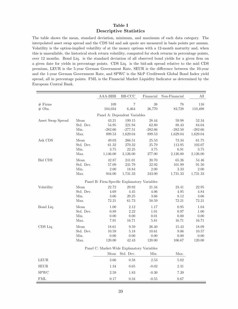
Table I
Descriptive Statistics
The table shows the mean, standard deviation, minimum, and maximum of each data category. The
interpolated asset swap spread and the CDS bid and ask quote are measured in basis points per annum.
Volatility is the option-implied volatility of at the money options with a 12-month maturity and, when
this is unavailable, the historical stock return volatility, computed for stock returns in percentage points,
over 12 months. Bond Liq. is the standard deviation of all observed bond yields for a given firm on
a given date for yields in percentage points. CDS Liq. is the bid-ask spread relative to the mid CDS
premium, LEUR is the 5-year German Government Rate, SEUR is the difference between the 10-year
and the 1-year German Government Rate, and SPWC is the S&P Creditweek Global Bond Index yield
spread, all in percentage points. FML is the Financial Market Liquidity Indicator as determined by the
European Central Bank.
AAA-BBB BB-CCC Financial Non-Financial All
# Firms 109 7 38 78 116# Obs. 104,034 6,464 26,770 83,728 110,498
Panel A: Dependent Variables
Asset Swap Spread Mean 43.21 199.15 28.44 59.98 52.34Std. Dev. 54.95 221.94 62.80 88.43 84.04Min. -282.66 -277.51 -282.66 -282.50 -282.66Max. 899.53 1,629.04 899.53 1,629.04 1,629.04
Ask CDS Mean 49.03 266.51 25.53 73.34 61.75Std. Dev. 61.32 270.32 25.79 113.95 102.07Min. 3.75 22.25 3.75 6.91 3.75Max. 1,146.00 2,126.00 277.00 2,126.00 2,126.00
Bid CDS Mean 42.87 241.01 20.70 65.26 54.46Std. Dev. 57.09 231.79 22.92 101.99 91.50Min. 2.00 18.84 2.00 3.33 2.00Max. 944.00 1,731.33 243.00 1,731.33 1,731.33
Panel B: Firm-Specific Explanatory Variables
Volatility Mean 22.72 29.92 21.34 23.41 22.95Std. Dev. 4.69 4.45 4.06 4.95 4.84Min. 3.66 20.25 3.66 8.12 3.66Max. 72.21 61.73 50.59 72.21 72.21
Bond Liq. Mean 1.00 2.12 1.17 0.95 1.04Std. Dev. 0.89 2.22 1.01 0.97 1.00Min. 0.00 0.00 0.01 0.00 0.00Max. 7.91 16.71 5.81 16.71 16.71
CDS Liq. Mean 18.61 9.59 26.40 15.43 18.09Std. Dev. 10.59 5.18 10.61 9.06 10.57Min. 0.00 0.00 0.00 0.00 0.00Max. 120.00 42.43 120.00 106.67 120.00
Panel C: Market-Wide Explanatory Variables
Mean Std. Dev. Min. Max.
LEUR 3.66 0.58 2.53 5.02
SEUR 1.34 0.65 -0.02 2.31
SPWC 2.59 1.83 -0.30 7.39
FML 0.17 0.34 -0.55 0.67
39

Table II
The Dynamic Relation of CDS Premia and Bond Asset Swap Spreads
The table shows the estimated coefficients for the vector error correction model in Equation (1). askt is
the asset swap interpolated to a 5-year maturity, cdsk,lt is the CDS ask (l = a) or bid (l = b) premiumfor a 5-year maturity. The dependent variables are the asset swap spread and CDS premium changes,the explanatory variables are the vector error correction terms (askt−βk,lcdsk,lt ) and the lagged changes.
βk,l denotes the cointegration coefficient, αk,las and αk,lcds the coefficient estimates of the error correctionterm. The top row displays the number of firms for which a) an identical order of integration could notbe rejected at the 10% level, b) the Johansen test could not reject cointegration of the time series at the10% level, c) the augmented Dickey-Fuller test could reject a unit root in the residuals of the VECM atthe 10% level. Coefficients are given for premia in basis points.
AAA-BBB BB-CCC Financial Non-Financial All
Panel A: Asset Swap / Ask CDS# sign 77 5 23 59 82Mean βk,a -1.28 -0.98 -1.10 -1.32 -1.26Std. Dev. βk,a 1.70 0.68 0.90 1.87 1.65
# sign. 70 4 21 53 74
Mean αk,aas -0.07 -0.03 -0.09 -0.07 -0.07
Std. Dev. αk,aas 0.10 0.05 0.08 0.10 0.10
# sign. 43 5 6 42 48
Mean αk,acds 0.03 0.03 0.03 0.03 0.03
Std. Dev.αk,acds 0.03 0.04 0.03 0.03 0.03Panel B: Asset Swap / Bid CDS
# sign 76 5 22 59 81Mean βk,b -1.35 -1.44 -1.24 -1.39 -1.35Std. Dev. βk,b 1.58 1.52 1.01 1.73 1.57
# sign. 69 4 20 53 73
Mean αk,bas -0.07 -0.03 -0.08 -0.06 -0.07
Std. Dev. αk,bas 0.10 0.05 0.09 0.10 0.10
# sign. 41 4 6 39 45
Mean αk,bcds 0.03 0.03 0.03 0.03 0.03
Std. Dev.αk,bcds 0.03 0.03 0.03 0.03 0.03
40
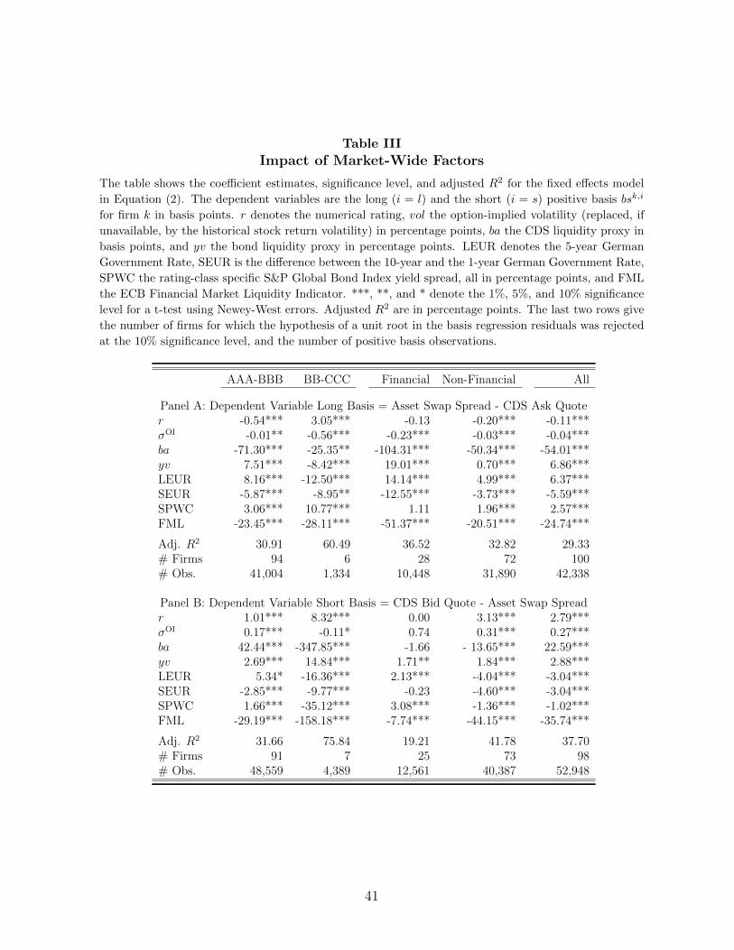
Table III
Impact of Market-Wide Factors
The table shows the coefficient estimates, significance level, and adjusted R2 for the fixed effects model
in Equation (2). The dependent variables are the long (i = l) and the short (i = s) positive basis bsk,i
for firm k in basis points. r denotes the numerical rating, vol the option-implied volatility (replaced, if
unavailable, by the historical stock return volatility) in percentage points, ba the CDS liquidity proxy in
basis points, and yv the bond liquidity proxy in percentage points. LEUR denotes the 5-year German
Government Rate, SEUR is the difference between the 10-year and the 1-year German Government Rate,
SPWC the rating-class specific S&P Global Bond Index yield spread, all in percentage points, and FML
the ECB Financial Market Liquidity Indicator. ***, **, and * denote the 1%, 5%, and 10% significance
level for a t-test using Newey-West errors. Adjusted R2 are in percentage points. The last two rows give
the number of firms for which the hypothesis of a unit root in the basis regression residuals was rejected
at the 10% significance level, and the number of positive basis observations.
AAA-BBB BB-CCC Financial Non-Financial All
Panel A: Dependent Variable Long Basis = Asset Swap Spread - CDS Ask Quoter -0.54*** 3.05*** -0.13 -0.20*** -0.11***σOI -0.01** -0.56*** -0.23*** -0.03*** -0.04***ba -71.30*** -25.35** -104.31*** -50.34*** -54.01***yv 7.51*** -8.42*** 19.01*** 0.70*** 6.86***LEUR 8.16*** -12.50*** 14.14*** 4.99*** 6.37***SEUR -5.87*** -8.95** -12.55*** -3.73*** -5.59***SPWC 3.06*** 10.77*** 1.11 1.96*** 2.57***FML -23.45*** -28.11*** -51.37*** -20.51*** -24.74***
Adj. R2 30.91 60.49 36.52 32.82 29.33# Firms 94 6 28 72 100# Obs. 41,004 1,334 10,448 31,890 42,338
Panel B: Dependent Variable Short Basis = CDS Bid Quote - Asset Swap Spreadr 1.01*** 8.32*** 0.00 3.13*** 2.79***σOI 0.17*** -0.11* 0.74 0.31*** 0.27***ba 42.44*** -347.85*** -1.66 - 13.65*** 22.59***yv 2.69*** 14.84*** 1.71** 1.84*** 2.88***LEUR 5.34* -16.36*** 2.13*** -4.04*** -3.04***SEUR -2.85*** -9.77*** -0.23 -4.60*** -3.04***SPWC 1.66*** -35.12*** 3.08*** -1.36*** -1.02***FML -29.19*** -158.18*** -7.74*** -44.15*** -35.74***
Adj. R2 31.66 75.84 19.21 41.78 37.70# Firms 91 7 25 73 98# Obs. 48,559 4,389 12,561 40,387 52,948
41

Table IV
Buy-and-Hold Basis Strategies
The table shows the mean, median, standard deviation, minimum, and maximum trading profit
in basis poinits for the long and short buy-and-hold basis trades. The entry trigger level e0 varies
between 10 bp and 100 bp, the transaction costs between 5% and 30% of the mid bond asset swap
spread. For the short basis trade, the shorting costs equal 40 bp p.a. The last rows give the number
of trades which were incepted under each strategy.
Entry Trigger
e0 = 10 bp e0 = 50 bp e0 = 100 bp
Panel A: Long Basis Trade
5% Transaction Costs Mean 225.38 816.53 1,173.52Median 106.39 628.66 908.52Std. Dev. 357.96 611.69 614.74Min. 54.25 264.30 525.46Max. 4,205.17 4,205.17 4,205.17# Trades 13,708 2,183 1,218
15% Transaction Costs Mean 310.81 924.51 1,257.37Median 148.38 728.00 1,071.82Std. Dev. 429.53 613.96 605.20Min. 61.61 296.22 578.66Max. 4,115.22 4,115.22 4,115.22# Trades 8,078 1,710 1,003
30% Transaction Costs Mean 483.57 1,090.24 1,402.30Median 250.63 853.63 1,302.81Std. Dev. 528.30 604.08 582.66Min. 81.61 359.11 702.07Max. 3,980.29 3,980.29 3,980.29# Trades 3,920 1,189 723
Panel B: Short Basis Trade
5% Transaction Costs Mean 528.66 775.44 1,030.19Median 350.53 702.57 995.86Std. Dev. 446.04 417.47 336.30Min. 50.88 251.78 502.21Max. 2,446.36 2,446.36 2,446.36# Trades 5,557 3,347 2,050
15% Transaction Costs Mean 559.06 823.03 1,058.59Median 377.63 793.22 1,031.52Std. Dev. 444.45 407.00 322.37Min. 53.98 251.56 501.93Max. 2,438.62 2,438.62 2,438.62# Trades 4,974 2,891 1,821
30% Transaction Costs Mean 591.21 877.88 1,085.34Median 419.85 875.84 1,062.09Std. Dev. 442.79 389.35 310.12Min. 53.71 255.18 508.28Max. 2,427.00 2,427.00 2,427.00# Trades 4,300 2,407 1,558
42

Table V
Dissolution-Risky Basis Strategies
The table shows the mean, median, standard deviation, minimum, and maximum trading profit
in basis points for the long and short basis trades that are subject to dissolution risk. The entry
trigger level e0 varies between 10 bp and 100 bp. In Panel A, the position is dissolved when the
reference date for the CDS contract changes. In Panel B, the position is dissolved when the 1-year
interest rate increases (for the long basis trade) or decreases (for the short basis trade) by 10 bp
overnight. In Panel C, the position is dissolved if the reverse basis exceeds the exit trigger eτ of
75 bp, 100 bp, or 125 bp, and the entry trigger equals 10 bp. The transaction costs equal 5% of
the mid bond asset swap spread. The shorting costs equal 40 bp p.a.
Entry Trigger
e0 = 10 bp e0 = 50 bp e0 = 100 bp
Panel A: Reference Date Change
Long Basis Trade Mean 8.55 38.00 37.64Median -8.01 7.43 6.36Std. Dev. 264.99 544.73 699.19Min. -3,526.90 -2,707.80 -2,707.80Max. 3,865.97 2,858.86 2,858.86
Short Basis Trade Mean -20.81 1.75 32.52Median -21.84 -24.82 -30.29Std. Dev. 397.08 455.97 490.83Min. -2,567.69 -2,375.00 -2,097.12Max. 1,733.76 1,733.76 1,733.76
Panel B: Interest Rate Shift
Long Basis Trade Mean 28.26 62.07 2.51Median 13.01 80.80 83.98Std. Dev. 271.87 639.64 821.46Min. -3,526.71 -2,705.30 -2,705.30Max. 3,148.06 3,148.06 3,148.06
Short Basis Trade Mean 9.91 49.18 168.92Median 29.69 44.42 113.15Std. Dev. 423.97 469.12 452.11Min. -2,356.40 -1,796.10 -1,674.69Max. 2,681.83 2,681.83 2,681.83
Panel C: Stop Loss Strategy
eτ = 75 bp eτ = 100 bp eτ = 125 bp
Long Basis Trade Mean 2.28 23.01 41.51Median 31.16 42.94 50.35Std. Dev. 123.89 130.03 122.57Min. -1,260.31 -1,260.31 -1,260.31Max. 342.02 422.13 536.58
Short Basis Trade Mean -81.68 -118.25 -167.93Median -71.37 -129.75 -135.94Std. Dev. 107.48 121.50 255.64Min. -665.99 -665.99 -1,042.37Max. 183.84 187.08 259.17
43

Table VI
Impact of Market-Wide Factors on Basis Trade Profits
The table shows the coefficient estimates, significance level, and adjusted R2 for the fixed effects
model in Equation (3). The dependent variables are the long (i = l) and the short (i = s) basis
trade profits pk,i for firm k in basis points, determined as in Table V. Panel A.1 and A.2 give the
results for the basis trades dissolved when the reference date changes, Panel B.1 and B.2 the basis
trades dissolved after an interest rate shock, and Panel C.1 and C.2 the basis trades dissolved
when the stop loss barrier is reached. r, ba, yv, LEUR, SEUR, SPWC, and FML are defined
as in Table III. ***, **, and * denote the 1%, 5%, and 10% significance level for a t-test using
Newey-West errors. Adjusted R2 are in percentage points.
AAA-BBB BB-CCC Financial Non-Financial All
Panel A: Exit Trigger Reference Date Change
Panel A.1: Dependent Variable = Long Basis Trade Profit
r 5.60*** 25.93*** 36.00*** 3.20*** 3.32***σOI -0.98*** -5.70*** -4.43*** -0.73*** -0.74***ba 215.83*** -1,715.61*** 1,609.20*** 20.31** 168.55***yv 77.44*** 39.51** 437.62*** 14.31*** 74.04***LEUR -90.04*** 440.28*** -439.47*** -36.25*** -77.60***SEUR -11.10* -54.40 180.68*** -13.42** -13.80**SPWC -73.75*** 46.13 -311.13*** -0.47 -69.92***FML -220.54*** -386.22*** -413.66*** -127.90*** -217.32***Adj. R2 (11.18) (27.58) (56.35) (3.57) (10.81)
Panel A.2: Dependent Variable = Short Basis Trade Profit
r -4.09*** -45.16*** -96.73*** -14.62*** -16.77***σOI 1.88*** 2.28*** -9.76*** 2.46*** 2.47***ba 454.46*** -5,752.31*** -1,808.42*** -764.58*** -455.23***yv 31.83*** -15.81** -409.07*** -47.11*** -44.12***LEUR -222.05*** -738.14*** -435.18*** -260.80*** -262.34***SEUR 22.66 111.78*** 196.62*** -63.80*** -23.30*SPWC -0.92 -496.78*** 162.77*** 0.63 1.78FML -217.63*** -811.59*** 752.60*** -302.70*** -140.73***Adj. R2 (8.61) (40.72) (44.94) (15.46) (14.97)
44
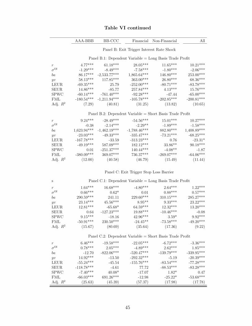
Table VI continued
AAA-BBB BB-CCC Financial Non-Financial All
Panel B: Exit Trigger Interest Rate Shock
Panel B.1: Dependent Variable = Long Basis Trade Profit
r 4.77*** 61.18*** 28.05*** 11.65*** 10.21***σOI -1.29*** -8.49*** -7.58*** -1.80*** -2.06***ba 86.17*** -2,533.77*** 1,865.64*** 146.80*** 253.00***yv 58.13*** 117.85*** 363.00*** 26.80*** 68.36***LEUR -69.35*** 25.79 -252.00*** -80.71*** -83.78***SEUR 14.86*** -85.77 257.84*** 4.13*** 15.76***SPWC -60.14*** -761.40*** -92.28*** -47.44 -65.00***FML -180.54*** -1,211.94*** -105.78*** -202.85*** -200.81***Adj. R2 (7.29) (40.81) (31.25) (13.82) (10.65)
Panel B.2: Dependent Variable = Short Basis Trade Profit
r 9.24*** -28.49*** -54.56*** 15.01*** 10.27***σOI -0.38 -2.14*** -2.29** -1.89*** -1.58***ba 1,623.94*** -1,462.19*** -1,788.46*** 882.80*** 1,408.89***yv -23.03*** -49.33*** -335.47*** -73.21*** -68.25***LEUR -167.78*** -33.59 -313.23*** 0.76 -23.31*SEUR -49.19*** 587.09*** 182.12*** 33.86** 90.18***SPWC 0.01 -251.37*** 140.44*** -4.08** -1.87FML -380.09*** 369.07*** 736.37*** -269.07*** -64.06***Adj. R2 (12.00) (40.58) (46.79) (15.49) (11.44)
Panel C: Exit Trigger Stop Loss Barrier
s Panel C.1: Dependent Variable = Long Basis Trade Profit
r 1.64*** 16.68*** -4.80*** 2.64*** 1.22***σOI 0.66*** 0.62* 0.01 0.88*** 0.57***ba 290.59*** 241.11 229.60*** 310.15*** 285.27***yv 23.14*** 45.56*** 8.95** 9.33*** 23.22***LEUR 12.81*** -65.68* 64.59*** 12.32*** 13.20***SEUR 0.64 -127.23*** 19.88*** -10.46*** -0.08SPWC 9.15*** -18.16 42.96*** 3.59* 9.92***FML -50.91*** 230.50*** -24.45** -73.58*** -49.20***Adj. R2 (15.67) (80.69) (35.64) (17.36) (9.22)
Panel C.2: Dependent Variable = Short Basis Trade Profit
r 6.46*** -19.58*** -22.05*** -6.72*** -3.36***σOI 0.78*** 2.05*** -4.89*** 2.62*** 1.85***ba -12.70 -822.06*** -520.47*** -139.79*** -339.95***yv 14.92*** -13.50 -292.32*** -5.19 -20.39***LEUR -55.24*** -45.54 -155.76*** -83.54*** -77.28***SEUR -118.78*** -4.61 77.72 -88.53*** -83.28***SPWC -7.40*** 40.08* -17.07 1.82* 0.47FML -66.03*** 691.26*** -12.98 -25.22* -53.68***Adj. R2 (25.63) (45.39) (57.37) (17.98) (17.78)
45

Table VII
Basis Strategies in the Financial Crisis
The table shows the mean, median, standard deviation, minimum, and maximum trading profit in
basis points for the long and short buy-and-hold basis trades (Panel A) and the dissolution-risky
basis trades (Panels B to D). The transaction costs equal 5% of the mid bond asset swap spread.
For the short basis trade, the shorting costs equal 40 bp p.a. The last rows give the number of
trades which were incepted under each strategy.
Long Basis Trade Short Basis Trade Long Basis Trade Short Basis Trade
Panel A: Buy-and-Hold Basis Trades
e0 = 10 bp e0 = 100 bpMean 343.72 380.42 964.27 1,258.66Median 201.30 201.78 801.56 949.70Std. Dev. 364.82 574.54 455.74 975.81Min. 56.87 50.42 539.45 503.67Max. 4,003.18 8,550.45 4,003.18 8,550.45# Trades 6,792 6,506 1,174 1,041
Panel B: Basis Trade Dissolved due to Reference Date Change
e0 = 10 bp e0 = 100 bpMean -21.42 -43.72 43.58 -86.18Median -29.73 -4.60 -11.41 11.02Std. Dev. 355.18 511.62 619.73 1,008.02Min. -2,270.11 -4,874.88 -1,735.95 -4,476.00Max. 5,315.73 3,395.37 5,315.73 3,395.37
Panel C: Basis Trade Dissolved due to Interest Rate Shock
e0 = 10 bp e0 = 100 bpMean -41.44 -50.07 -28.96 -102.42Median -29.20 -31.61 -44.84 -75.84Std. Dev. 193.21 422.33 378.49 899.36Min. -1,942.10 -4,773.29 -1,186.30 -3,459.18Max. 4,065.53 7,151.38 4,065.53 7,151.38
# Trades 6,792 6,486 1,174 1,090Panel D: Basis Trade Dissolved due to Stop Loss Strategy
eτ = 75 bp eτ = 125 bpMean -199.08 -104.95 -254.43 -226.51Median -200.02 -98.11 -309.71 -257.58Std. Dev. 134.11 75.91 225.82 167.06Min. -814.87 -1,511.25 -976.44 -1,511.25Max. 30.50 28.31 109.55 60.30
# Trades 1,660 1,949 4,377 4,475
46

Table VIII
Value at Risk and Expected Shortfall
The table shows the value at risk (VaR) and expected shortfall (ES) in basis points of the trading
profit for the long and short basis trades that are subject to dissolution risk. VaR and ES are
determined at the 10%, 5%, and 1% level. The transaction costs equal 5% of the mid bond asset
swap spread. For the short basis trade, the shorting costs equal 40 bp p.a.
Pre-Crisis In Crisis Pre-Crisis In Crisis
e0=10 bp e0=100 bp
Panel A: Basis Trade Dissolved due to Reference Date Change
Long Basis Trade VaR 10% -72.63 -259.73 -514.17 -556.945% -127.84 -453.92 -859.97 -758.041% -551.13 -837.83 -2,385.23 -1,589.21
ES 10% -279.97 -562.48 -1,429.26 -911.795% -466.26 -789.98 -2,167.79 -1,184.921% -1,398.72 -1,519.17 -2,559.33 -1,668.49
Short Basis Trade VaR 10% -395.53 -408.12 -410.02 -1,127.815% -589.09 -739.02 -584.37 -1,664.201% -1,335.40 -1,828.59 -1,651.58 -3,750.26
ES 10% -757.39 -1,023.42 -792.03 -2,231.205% -1,031.02 -1,524.55 -1,100.18 -3,134.551% -1,942.20 -3,030.91 -1,910.98 -4,089.35
Panel B: Basis Trade Dissolved due to Interest Rate Shock
Long Basis Trade VaR 10% -251.53 -144.37 -906.92 -234.485% -314.48 -242.87 -1,870.86 -351.411% -1,047.19 -596.45 -2,381.89 -994.74
ES 10% -523.98 -317.63 -1,843.66 -472.575% -774.74 -452.12 -2,253.36 -666.391% -1,947.70 -890.24 -2,556.47 -1,174.67
Short Basis Trade VaR 10% -582.91 -292.55 -291.10 -912.005% -730.60 -513.75 -389.52 -1,408.651% -921.14 -1,380.69 -897.34 -2,111.02
ES 10% -774.26 -713.07 -501.98 -1,553.325% -900.39 -1,031.56 -665.69 -1,965.641% -1,327.07 -2,034.96 -1,272.70 -2,548.41
Panel C: Basis Trade Dissolved due to Stop Loss Strategy
eτ=75 bp eτ=125 bp
Long Basis Trade VaR 10% -198.16 -319.41 0.71 -542.425% -252.17 -476.75 -227.73 -590.791% -362.01 -645.97 -382.77 -667.58
ES 10% -275.26 -474.44 -238.39 -604.715% -327.89 -588.91 -342.62 -643.711% -483.65 -696.43 -537.71 -728.08
Short Basis Trade VaR 10% -169.03 -162.53 -448.22 -402.135% -318.18 -193.67 -858.27 -455.021% -502.48 -358.83 -976.11 -578.10
ES 10% -339.88 -243.10 -751.89 -491.725% -398.28 -309.02 -941.44 -560.081% -615.63 -571.99 -999.15 -799.96
47
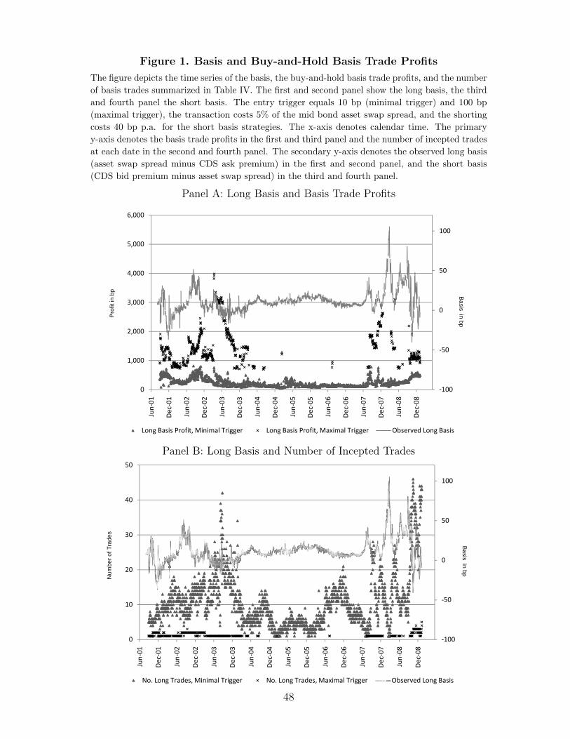
Figure 1. Basis and Buy-and-Hold Basis Trade Profits
The figure depicts the time series of the basis, the buy-and-hold basis trade profits, and the number
of basis trades summarized in Table IV. The first and second panel show the long basis, the third
and fourth panel the short basis. The entry trigger equals 10 bp (minimal trigger) and 100 bp
(maximal trigger), the transaction costs 5% of the mid bond asset swap spread, and the shorting
costs 40 bp p.a. for the short basis strategies. The x-axis denotes calendar time. The primary
y-axis denotes the basis trade profits in the first and third panel and the number of incepted trades
at each date in the second and fourth panel. The secondary y-axis denotes the observed long basis
(asset swap spread minus CDS ask premium) in the first and second panel, and the short basis
(CDS bid premium minus asset swap spread) in the third and fourth panel.
Panel A: Long Basis and Basis Trade Profits
0
50
100
2,000
3,000
4,000
5,000
6,000
Pro
fit in
bp
Ba
sis in b
p
‐100
‐50
0
50
100
0
1,000
2,000
3,000
4,000
5,000
6,000
Jun‐01
Dec‐01
Jun‐02
Dec‐02
Jun‐03
Dec‐03
Jun‐04
Dec‐04
Jun‐05
Dec‐05
Jun‐06
Dec‐06
Jun‐07
Dec‐07
Jun‐08
Dec‐08
Long Basis Profit, Minimal Trigger Long Basis Profit, Maximal Trigger Observed Long Basis
Pro
fit in
bp
Ba
sis in b
p
Panel B: Long Basis and Number of Incepted Trades
0
50
100
20
30
40
50
Nu
mb
er
of T
rad
es
Ba
sis in bp
‐100
‐50
0
50
100
0
10
20
30
40
50
Jun‐01
Dec‐01
Jun‐02
Dec‐02
Jun‐03
Dec‐03
Jun‐04
Dec‐04
Jun‐05
Dec‐05
Jun‐06
Dec‐06
Jun‐07
Dec‐07
Jun‐08
Dec‐08
No. Long Trades, Minimal Trigger No. Long Trades, Maximal Trigger Observed Long Basis
Nu
mb
er
of T
rad
es
Ba
sis in bp
48
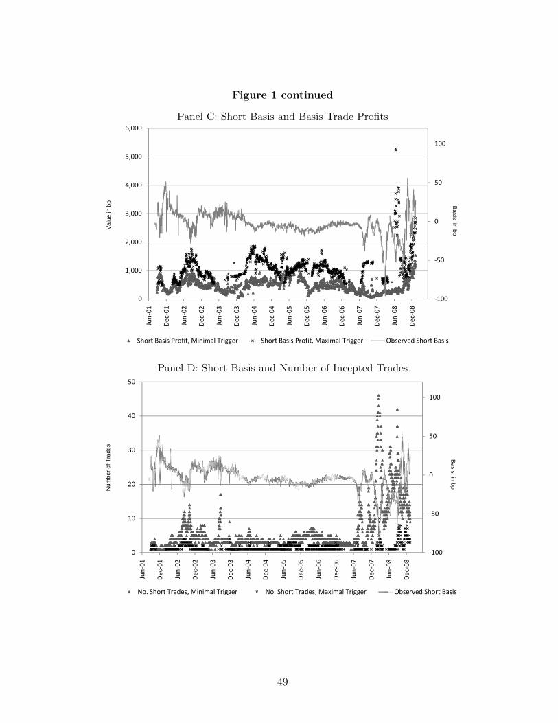
Figure 1 continued
Panel C: Short Basis and Basis Trade Profits
0
50
100
2,000
3,000
4,000
5,000
6,000
Va
lue
in b
p Ba
sis in bp
‐100
‐50
0
50
100
0
1,000
2,000
3,000
4,000
5,000
6,000
Jun‐01
Dec‐01
Jun‐02
Dec‐02
Jun‐03
Dec‐03
Jun‐04
Dec‐04
Jun‐05
Dec‐05
Jun‐06
Dec‐06
Jun‐07
Dec‐07
Jun‐08
Dec‐08
Short Basis Profit, Minimal Trigger Short Basis Profit, Maximal Trigger Observed Short Basis
Va
lue
in b
p Ba
sis in bp
Panel D: Short Basis and Number of Incepted Trades
0
50
100
20
30
40
50
Nu
mb
er
of
Tra
de
sB
asis in
bp
‐100
‐50
0
50
100
0
10
20
30
40
50
Jun‐01
Dec‐01
Jun‐02
Dec‐02
Jun‐03
Dec‐03
Jun‐04
Dec‐04
Jun‐05
Dec‐05
Jun‐06
Dec‐06
Jun‐07
Dec‐07
Jun‐08
Dec‐08
No. Short Trades, Minimal Trigger No. Short Trades, Maximal Trigger Observed Short Basis
Nu
mb
er
of
Tra
de
sB
asis in
bp
49
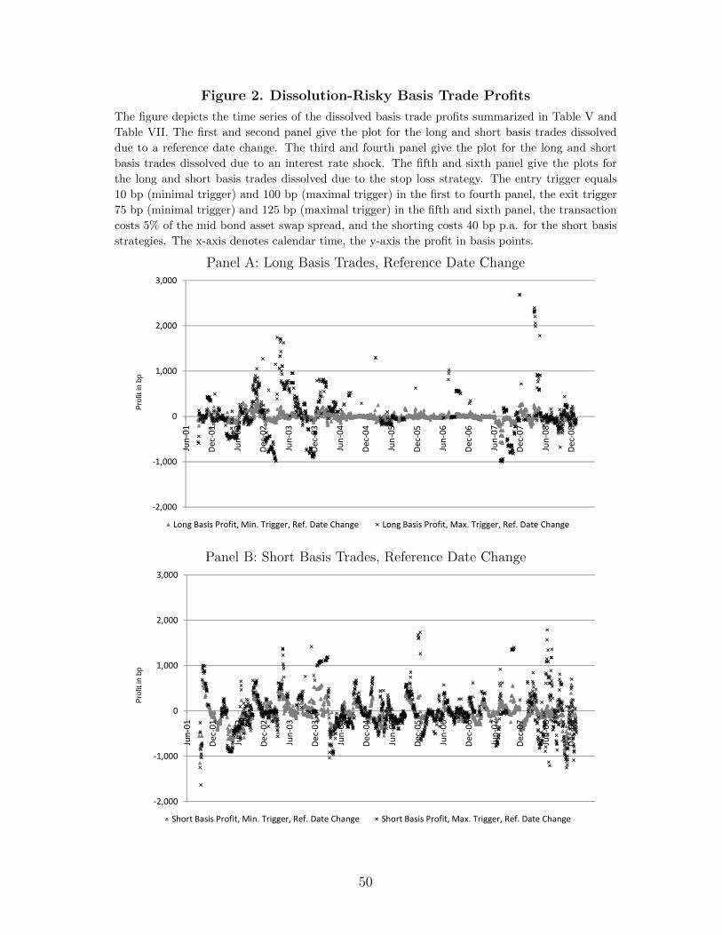
Figure 2. Dissolution-Risky Basis Trade Profits
The figure depicts the time series of the dissolved basis trade profits summarized in Table V and
Table VII. The first and second panel give the plot for the long and short basis trades dissolved
due to a reference date change. The third and fourth panel give the plot for the long and short
basis trades dissolved due to an interest rate shock. The fifth and sixth panel give the plots for
the long and short basis trades dissolved due to the stop loss strategy. The entry trigger equals
10 bp (minimal trigger) and 100 bp (maximal trigger) in the first to fourth panel, the exit trigger
75 bp (minimal trigger) and 125 bp (maximal trigger) in the fifth and sixth panel, the transaction
costs 5% of the mid bond asset swap spread, and the shorting costs 40 bp p.a. for the short basis
strategies. The x-axis denotes calendar time, the y-axis the profit in basis points.
Panel A: Long Basis Trades, Reference Date Change
0
1,000
2,000
3,000
01
01 02
02 03
03 04
04 05
05 06
06 07
07 08
08
Pro
fit in
bp
‐2,000
‐1,000
0
1,000
2,000
3,000
Jun‐01
Dec‐01
Jun‐02
Dec‐02
Jun‐03
Dec‐03
Jun‐04
Dec‐04
Jun‐05
Dec‐05
Jun‐06
Dec‐06
Jun‐07
Dec‐07
Jun‐08
Dec‐08
Long Basis Profit, Min. Trigger, Ref. Date Change Long Basis Profit, Max. Trigger, Ref. Date Change
Pro
fit in
bp
Panel B: Short Basis Trades, Reference Date Change
0
1,000
2,000
3,000
01
01 02
02 03
03 04
04 05
05 06
06 07
07 08
08
Pro
fit in
bp
‐2,000
‐1,000
0
1,000
2,000
3,000
Jun‐01
Dec‐01
Jun‐02
Dec‐02
Jun‐03
Dec‐03
Jun‐04
Dec‐04
Jun‐05
Dec‐05
Jun‐06
Dec‐06
Jun‐07
Dec‐07
Jun‐08
Dec‐08
Short Basis Profit, Min. Trigger, Ref. Date Change Short Basis Profit, Max. Trigger, Ref. Date Change
Pro
fit in
bp
50

Figure 2 continued
Panel C: Long Basis Trades, Interest Rate Shock
0
1,000
2,000
3,00001
01 02
02 03
03 04
04 05
05 06
06 07
07 08
08
Pro
fit in
bp
‐2,000
‐1,000
0
1,000
2,000
3,000Jun‐01
Dec‐01
Jun‐02
Dec‐02
Jun‐03
Dec‐03
Jun‐04
Dec‐04
Jun‐05
Dec‐05
Jun‐06
Dec‐06
Jun‐07
Dec‐07
Jun‐08
Dec‐08
Long Basis Profit, Min. Trigger, Inter. Rate Shock Long Basis Profit, Max. Trigger, Int. Rate Shock
Pro
fit in
bp
Panel D: Short Basis Trades, Interest Rate Shock
0
1,000
2,000
3,000
01
01 02
02 03
03 04
04 05
05 06
06 07
07 08
08
Pro
fit in
bp
‐2,000
‐1,000
0
1,000
2,000
3,000
Jun‐01
Dec‐01
Jun‐02
Dec‐02
Jun‐03
Dec‐03
Jun‐04
Dec‐04
Jun‐05
Dec‐05
Jun‐06
Dec‐06
Jun‐07
Dec‐07
Jun‐08
Dec‐08
Short Basis Profit, Min. Trigger, Int. Rate Shock Short Basis Profit, Max. Trigger, Int. Rate Shock
Pro
fit in
bp
51

Figure 2 continued
Panel E: Long Basis Trades, Stop Loss Strategy
‐200
0
200
400Jun‐01
Dec‐01
Jun‐02
Dec‐02
Jun‐03
Dec‐03
Jun‐04
Dec‐04
Jun‐05
Dec‐05
Jun‐06
Dec‐06
Jun‐07
Dec‐07
Jun‐08
Dec‐08
Pro
fit in
bp
‐600
‐400
‐200
0
200
400Jun‐01
Dec‐01
Jun‐02
Dec‐02
Jun‐03
Dec‐03
Jun‐04
Dec‐04
Jun‐05
Dec‐05
Jun‐06
Dec‐06
Jun‐07
Dec‐07
Jun‐08
Dec‐08
Long Basis Profit, Min. Exit Trigger, Stop Loss Long Basis Profit, Max. Exit Trigger, Stop Loss
Pro
fit in
bp
Panel F: Short Basis Trades, Stop Loss Strategy
‐200
0
200
400
Jun‐01
Dec‐01
Jun‐02
Dec‐02
Jun‐03
Dec‐03
Jun‐04
Dec‐04
Jun‐05
Dec‐05
Jun‐06
Dec‐06
Jun‐07
Dec‐07
Jun‐08
Dec‐08
Pro
fit in
bp
‐600
‐400
‐200
0
200
400
Jun‐01
Dec‐01
Jun‐02
Dec‐02
Jun‐03
Dec‐03
Jun‐04
Dec‐04
Jun‐05
Dec‐05
Jun‐06
Dec‐06
Jun‐07
Dec‐07
Jun‐08
Dec‐08
Short Basis Profit, Min. Exit Trigger, Stop Loss Short Basis Profit, Max. Exit Trigger, Stop Loss
Pro
fit in
bp
52

Figure 3. Basis Trade Profit Distribution
The figure depicts the relative frequency of the basis trade profits summarized in Table V and
Table VII. The first and second panel give the plot for the long and short basis trade profits
dissolved due to a reference date change before and during the financial crisis (pre and post June
2007). The third and fourth panel give the plot for the long and short basis trade profits dissolved
due to an interest rate shock. The fifth and sixth panel give the plots for the long and short basis
trade profits dissolved due to the stop loss strategy. The x-axis gives the profit in basis points, the
y-axis the relative frequency with which the profit was observed.
Panel A: Long Basis Trades, Reference Date Change
0
0.1
0.2
0.3
0.4
0.5
0.6
0.7
0.8
0.9
-1,500 -1,000 -500 0 500 1,000 1,500
Long Strategy, Pre-Crisis, Entry Trigger 10 bp, Reference Date Change
Long Strategy, In Crisis, Entry Trigger 10 bp, Reference Date Change
Long Strategy, Pre-Crisis, Entry Trigger 100 bp, Reference Date Change
Long Strategy, In Crisis, Entry Trigger 100 bp, Reference Date Change
Panel B: Short Basis Trades, Reference Date Change
0
0.05
0.1
0.15
0.2
0.25
-1,500 -1,000 -500 0 500 1,000 1,500
Short Strategy, Pre-Crisis, Entry Trigger 10 bp, Reference Date Change
Short Strategy, In Crisis, Entry Trigger 10 bp, Reference Date Change
Short Strategy, Pre-Crisis, Entry Trigger 100 bp, Reference Date Change
Short Strategy, In Crisis, Entry Trigger 100 bp, Reference Date Change
53
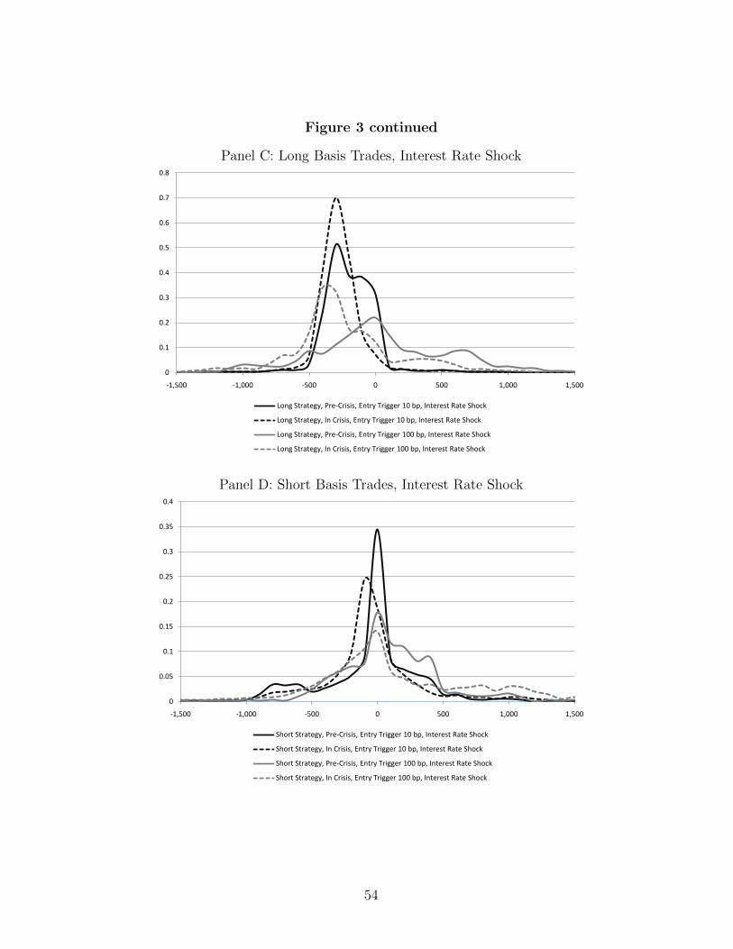
Figure 3 continued
Panel C: Long Basis Trades, Interest Rate Shock
0
0.1
0.2
0.3
0.4
0.5
0.6
0.7
0.8
-1,500 -1,000 -500 0 500 1,000 1,500
Long Strategy, Pre-Crisis, Entry Trigger 10 bp, Interest Rate Shock
Long Strategy, In Crisis, Entry Trigger 10 bp, Interest Rate Shock
Long Strategy, Pre-Crisis, Entry Trigger 100 bp, Interest Rate Shock
Long Strategy, In Crisis, Entry Trigger 100 bp, Interest Rate Shock
Panel D: Short Basis Trades, Interest Rate Shock
0
0.05
0.1
0.15
0.2
0.25
0.3
0.35
0.4
-1,500 -1,000 -500 0 500 1,000 1,500
Short Strategy, Pre-Crisis, Entry Trigger 10 bp, Interest Rate Shock
Short Strategy, In Crisis, Entry Trigger 10 bp, Interest Rate Shock
Short Strategy, Pre-Crisis, Entry Trigger 100 bp, Interest Rate Shock
Short Strategy, In Crisis, Entry Trigger 100 bp, Interest Rate Shock
54
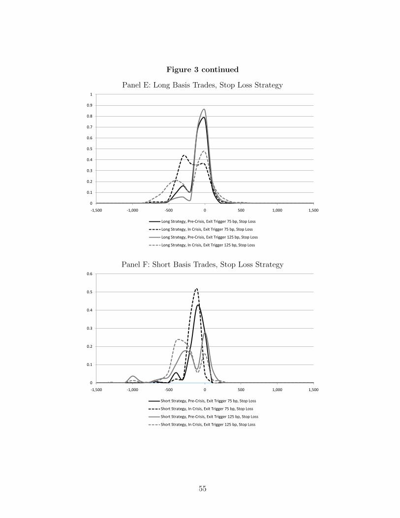
Figure 3 continued
Panel E: Long Basis Trades, Stop Loss Strategy
0
0.1
0.2
0.3
0.4
0.5
0.6
0.7
0.8
0.9
1
-1,500 -1,000 -500 0 500 1,000 1,500
Long Strategy, Pre-Crisis, Exit Trigger 75 bp, Stop Loss
Long Strategy, In Crisis, Exit Trigger 75 bp, Stop Loss
Long Strategy, Pre-Crisis, Exit Trigger 125 bp, Stop Loss
Long Strategy, In Crisis, Exit Trigger 125 bp, Stop Loss
Panel F: Short Basis Trades, Stop Loss Strategy
0
0.1
0.2
0.3
0.4
0.5
0.6
-1,500 -1,000 -500 0 500 1,000 1,500
Short Strategy, Pre-Crisis, Exit Trigger 75 bp, Stop Loss
Short Strategy, In Crisis, Exit Trigger 75 bp, Stop Loss
Short Strategy, Pre-Crisis, Exit Trigger 125 bp, Stop Loss
Short Strategy, In Crisis, Exit Trigger 125 bp, Stop Loss
55


