
Title: Large Area Scene Selection Interface (LASSI). Methodology of Selecting LandsatImagery for the Global Land Survey 2005.
Description: To facilitate the scene selection process for the GLS2005, NASA and theUSGS sponsored the development of a new tool to generate optimal collections ofimagery using metadata statistics and user-defined weighting criteria.
The authors on the paper are:
Shannon FranksStinger Ghaffarian Technologies, Inc. (SGT)i
Goddard Space Flight Center (Code 614.4)Greenbelt, MD 20771
Shannon.franks(a,,nasa.Qov, (301) 614-6682
Jeffrey G. MasekNASA Goddard Space Flight Center
Biospheric Sciences Branch (Code 614.4)Greenbelt, MD 20771
Jeffery. G.Masek(a^nasa. 2ov
Rachel M. K. HeadleyUSGS Center for Earth Resources Observation and Science (EROS)
47914 252nd StreetSioux Falls, SD 57198
rheadle a,usgs.gov
John GaschEmalico LLC
Goddard Space Flight Center (Code 428.1)Greenbelt, MD 20771
John.R.Gasch(a nasa.gov
Terry ArvidsonLockheed Martin
Goddard Space Flight Center (Code 614.4)Greenbelt, MD 20771
terry. arvidson(a^.nasa. gov
' This work was done while Mr. Franks was an employee of the University ofMaryland/Geography Department.
https://ntrs.nasa.gov/search.jsp?R=20090027892 2018-08-02T09:32:54+00:00Z

Abstract
The Global Land Survey (GLS) 2005 is a cloud-free, orthorectified collection of Landsat
imagery acquired during the 2004-2007 epoch intended to support global land-cover and
ecological monitoring. Due to the numerous complexities in selecting imagery for the
GLS2005, NASA and the U.S. Geological Survey (USGS) sponsored the development of
an automated scene selection tool, the Large Area Scene Selection Interface (LASSI), to
aid in the selection of imagery for this data set. This innovative approach to scene
selection applied a user-defined weighting system to various scene parameters: image
cloud cover, image vegetation greenness, choice of sensor, and the ability of the Landsat
7 Scan Line Corrector (SLC)-off pair to completely fill image gaps, among others. The
parameters considered in scene selection were weighted according to their relative
importance to the data set, along with the algorithm's sensitivity to that weight. This
paper describes the methodology and analysis that established the parameter weighting
strategy, as well as the post-screening processes used in selecting the optimal data set for
GLS2005.
Introduction
Monitoring global changes in land cover is a principal objective of remote sensing
science. In order to produce reliable measures of land-cover change and disturbance,
researchers require a consistent global baseline set of cloud-free, leaf-on imagery. The
Global Land Survey (GLS — formerly known as "Geocover") data sets provide wall-to-
wall, cloud-free Landsat coverage of the Earth's land areas for epochs centered on 1975,
2

1990, 2000, and 2005. These data sets provide the science and conservation communities
a comprehensive view of how the planet's land areas have changed over the past thirty-
five years.
The goal of the Global Land Survey 2005 2 (GLS2005) was to provide one clear
Landsat or Landsat-like image during peak vegetation conditions for every location of the
global land area during the 2004-2007 period (Gutman et a1., 2008). The GLS2005 data
set consists of approximately 9,500 Landsat images; an increase compared to the 1990
GeoCoverTM (7,000 scenes) and the 2000 GeoCoverTM (8,200 scenes). This increase
accounts for additional coastal and island areas not represented in the earlier GeoCoverTM
data sets, and the inclusion of the Landsat Image Mosaic of Antarctica (LIMA) that was
produced separately in support of the International Polar Year.
GLS2005 was a collaborative effort between NASA and USGS, led by a science
steering group with members from NASA headquarters, NASA Goddard Space Flight
Center, USGS headquarters, USGS EROS, University of Maryland, Aerospace
Corporation, Lockheed Martin, and Emalico LLC.
The primary application of the GLS data sets are to monitor land use and land
cover changes over time at a moderate-resolution scale. In the interest of consistency
with the previous GLS data sets, the GLS science steering group preferred Landsat data
wherever possible. The majority of the global data set would be chosen from available
2 The GeoCoverT'I 2000 data set has been reprocessed to improve the geometric accuracy and
establish a control baseline for GLS2005, the other GeoCover TM data sets, and current Landsat product
generation. After reprocessing, the GeoCoverT`I data sets are renamed GLS.

Landsat 5 and Landsat 7 data using the LASSI tool, augmented by manually selecting (ie.
Not using LASSI imagery from Earth Observing 1's Advanced Land Imager (EO-1 ALI)
imagery and Terra Advanced Spaceborne Thermal Emission and Reflection Radiometer
(ASTER) as needed. This not only reflects the diversity of Landsat-like resolution
remote sensing satellites in orbit, but also underscores the shortcomings of Landsat: the
inability to secure global coverage with Landsat 5 Thematic Mapper (TM), and the
failure of the Landsat 7 Enhanced Thematic Mapper Plus (ETM+) Scan Line Corrector
(SLC) in 2003 (Gutman et al., 2008).
This paper describes the process of scene selection for the GLS2005 data set. To
facilitate the automation of the scene selection process, the GLS2005 project, in
collaboration with NASA Ames Research Center, developed a new tool to generate
optimal collections of imagery using metadata statistics and user-defined weighting
criteria. In the sections below, we describe the parameters used in scene selection,
discuss the reasoning behind the weighting of those parameters, talk briefly about the
post screening processes, show the results of the scene selection of North America, and
discuss lessons learned along the way.
Background
There are three existing global survey data sets: GeoCoverTM 1975, 1990, and 2000.
These were produced by the EarthSat Corporation (now MDA Federal, Inc.) under
contract to NASA. Scene selection for these data sets was based on visual aspects of the
imagery, like clouds, haze, missing scan lines, and other manifestations of poor data
4

quality. Image characteristics were weighed against the year and season in which the
data were acquired (Tucker et al., 2004). While scene selection was labor intensive, it
was feasible because only a few characteristics were considered, and most of them were
assessed quickly mainly by visual inspection. For GLS2005, not only were there more
data available, but the task became considerably more complicated due to the failure of
the Landsat 7 ETM+ SLC in 2003 (Williams et al., 2006). While there have been other
studies that have documented the methods of optimally putting together a Landsat 7
ETM+ large area database (Yang et al., 2001), none of these have addressed the
difficulties of gap filling imagery and have considered so many parameters in doing so.
Landsat 7 continues to acquire global coverage, but with the SLC failure each
scene is missing approximately 22 percent of its area coverage in cross-track, bow-tie
shape that are widest at the scene edges. The most suitable workaround for these missing
data in ETM+ images is to "gap fill" the imagery with other imagery from the same
growing season. Although this is a credible strategy (Masek, 2007), it magnifies the
complexity of the scene selection process. It was necessary to not only select the best
base scene for that World`vide Reference System (WRS) path and row, but also the best
associated fill scene. The pair of chosen images are referred to as the "base" and "fill"
selections. Occasionally, two fill images were chosen to achieve full geographic
coverage of the scene. The added complexities of dealing with gap-filled imagery did
raise the question of whether Landsat 7 ETM+ data should be used for the dataset. The
GLS2005 science steering group and user community representatives decided that, in
situations where the "base" and "fill" scenes were cloud-free and the land cover was not a

seasonally dynamic land cover type such as agriculture, it was preferable to use Landsat 7
"gap-filled" imagery due to its superior geometry and radiometry when compared to
Landsat 5 TM.
GLS2005 primarily consists of Landsat 5 TM and Landsat 7 ETM+ imagery with
supplemental selections from EO-1 ALI and Terra ASTER image collections. Given the
smaller swath-width of the ALI instrument (30km), EO-1 selections were limited to
coverage of small islands and reefs. ASTER imagery was used to fill in some
problematic regions, such as Northern Eurasia, where no suitable Landsat data were
available.
Large Area Scene Selection Interface Tool
Roughly 400,000 Landsat images were considered in scene selection by the
LASSI tool for GLS2005. These were reduced to 6119,500 WRS locations (referred to
hereafter as "scenes") based upon criteria that included acquisition date, cloud
contamination, gap-fill coverage, sensor choice, and geographic uniformity, as well as
other minor factors. To handle the large number of images in the selection pool, and the
increased complexities in scene selection for GLS2005, NASA Goddard Space Flight
Center (GSFC) and USGS Earth Resources Observation and Science Center (EROS)
sponsored the creation of an automated scene selection tool, known as LASSI. At the
heart of LASSI is an artificial-intelligence engine called the Global Map Generator
(GMG), which was developed by the Computational Sciences Division of NASA Ames
Research Center. GMG applies non-linear optimization to identify the "best' collection
of scenes based on a user-defined weighting system to pre-determined scene parameters.
6

The weighting system of the parameters was subjective in nature, but supported by
numerous trial and error attempts, along with consultation with the steering group and
professionals that have specific knowledge of the region (for example, professionals that
work in polar regions recommended to us that imagery that is later in the growing season
is more useful than imagery early in the growing season). "Relative importance" was
determined in a fashion that would maintain consistency with the goals of the data set.
With supplied metadata of all candidate images, GMG quickly and systematically sorts
through thousands of images to select the best overall set to form a regional solution. For
the sake of simplicity, this paper describes the methods used for establishing the
parameter weights specifically applied to the North American continent. For details
about the weighting scheme used for the other continents and the results of those
selections, please contact the authors directly. For more information on the algorithmic
basis for the tool, see Khatib et al. (2007).
Selection Parameters
Description
During scene selection, there were 14 parameters considered by LASSI. The weight of
each parameter was set by the LASSI operator to reflect its significance for scene
selection for a particular region. These factors and their associated weightings drove the
scene selection. All Landsat 7 imagery required image pairs to provide complete
coverage. A "base" image covers approximately 78 percent of the WRS scene area. The
7

"fill" image is chosen to furnish coverage of some or the entire remaining 22 percent gap
left by the base image. Fill image parameters apply only to Landsat 7.
• NDVI- base Image: Phenological Normalized Difference Vegetation Index
(NDVI) of Landsat 5 (L5) image or Landsat 7 (L7) base image, temporally
interpolated from a mean monthly NDVI record. For this factor, the
Pathfinder (PALS) AVHRR NDVI time series was used after sub-averaging
81,m resolution monthly values to the area of each WRS scene (James and
Kalluri, 1994).
• NDVI- fill Image: NDVI of the L7 fill image.
• ACCA- base Image: The Automated Cloud Cover Assessment (ACCA) score
is generated during L7 image processing and reports the percentage of clouds
present in the L7 imagery at a precision of 1% cloud cover. The L7 ACCA
algorithm is an unsupervised classifier that detects and reports clouds based
on the known spectral properties of clouds (Irish et al., 2006). L7 "ACCA
clouds" are defined as optimally thick or opaque, and does not include semi-
transparent clouds such as Cirrus, nor artifacts such as cloud edges or
shadows. The cloud score algorithm for L5 results in a coarser estimate (10%
cloud cover increments). For GLS2005, all L5 imagery was manually
prescreened to only consider cloud-free images. Increasing this weight
favored clear ETM+ base imagery or clear TM images.
• ACCA- fill Image: ACCA score for L7 fill image.
8

• Difference in Acquisition Dates between L7 gap-filled pairs: Increasing this
parameter favored L7 base/fill pairs with minimal seasonal difference between
them. As a side effect, this favors L5 imagery because the "date difference" is
zero. This factor was influential in regions where vegetation changed rapidly,
such as agricultural fields or regions with short growing seasons.
• Difference in Acquisition Dates between L7 gap-filled pairs (over
agriculture): This parameter worked in conjunction with the previous one, but
was applicable only for scenes containing a significant area of agriculture, as
defined by the MODIS landcover product, MOD 12 (LPDAAC, 2001). In
essence, it increased the effect of the parameter "Difference in acquisition
dates between L7 gap-filled pairs", scaled to the percent of the scene
agriculture area. An example of this parameter's influence can be found in the
section detailing parameter weighting.
• Area coverage: This factor influenced how much of the scene area was
covered by Landsat imagery. An L5 image always covers 100 percent of the
scene area. A single L7 image only covers 78 percent of the area, but a
composite of two L7 images achieves between 78% and 100% coverage.
Increasing this factor drove LASSI to select L7 image pairs that achieved as
close to 100 percent coverage as possible, or to select an L5 image instead.
• Difference in Day of Year between North-South neighbors: This parameter
weighted the preference of choosing images in adjacent north-south scenes
taken at the same time of year, irrespective of the specific year. Optimizing
9
this factor resulted in more compatible seasonality among neighboring scenes
in the north-south direction.
• Difference in Day of Year between East-West neighbors: Same as the above
parameter, but applied to the east-west neighboring scenes.
• Preference Landsat 5 Imagery: Increasing this parameter favored LASSI
selection of L5 imagery.
• Preference Landsat 7 Imagery: Increasing this parameter favored LASSI
selection of L7 imagery.
• Sensor Homogeneity: Increasing this parameter favored contiguous spatial
groups of a single sensor (L5 or L7). It is this parameter, along with the
Difference in Day of Year between the North-South and East-West neighbors
that encouraged uniformity of the resultant data set.
• Preference toward a Specific Date Range: For GLS2005, it was desirable to
select images acquired during the middle of the decade (2005 and 2006) as
opposed to 2004 and 2007. Increasing the weighting of this parameter
influenced that decision.
• Preference Day of Year: This parameter applies a preference toward selecting
images from the same time of year as the GeocoverTM 2000 data set. This
facilitates change-over-time research between the two datasets.
Parameter Weighting (with Metadata Visualizations)
Table 1 shows the weighting values used for the North American continent scene
selection. The scene selection for other continents used slightly different weights to adapt
10

to the differing characteristics of those regions. The numerical values are unitless and
simply express the relative weights assigned to various data set characteristics (explained
below).
Table 1. Parameter weightings used for North America scene selection for GLS2005.
Parameter Value Description
NDVI_B 60 NDVI — base image
NDVI_F 30 NDVI — fill image
ACCA_B 20 ACCA — base image
ACCA_F 20 ACCA — fill image
difAD_P 10 Difference in acquisition dates between L7 gap-filled pairs
difAD_P (ag) 40 Diff. in acquisition dates between L7 gap-filled pairs (over
agriculture)
Coverage _P 15 Area coverage
difDY_NS 4 Diff. in day of year between N-S neighbors
difDY_EW 4 Diff. in day of year between E-W neighbors
LS_pref 0 Preference L5 imagery
L7_pref 10 Preference L7 imagery
SensHomg 5 Sensor homogeneity
Date pref 10 Preference towards a specific date range (2005 and 2006)
DOY—Pref 15 Preference day of year (Geocover 2000 TM
11

ND VI - base and fill Images
Maximizing the NDVI of the base and fill images was given the greatest weight, since
imagery at the peak of the growing season is critical for land-cover and land-use change
analysis, which is the principal use of the GLS data sets. Plate 1 a depicts the NDVI
values, which have been scaled to represent the percent of maximum NDVI for each
scene. By displaying the map as percent of maximum made it easier to determine if the
parameter was successfully optimized. Normalizing the values facilitated comparison of
scenes with a low NDVI average (e.g., deserts) and scenes of high average NDVI. The
fill image was also strongly weighted to minimize the differences between the NDVI
values of the Landsat 7 gap-filled image pairs, as shown in Plate lb. This also ensured
that both images were acquired within the same growing season. The average absolute
NDVI for the base (Landsat 7 and Landsat 5) images was 0.560. In Plate 1, white is
ideal, and light-green is acceptable.
12

P'J
-AP I
0.65
0.6
7A Ar0.75
07
0.65p' 06
-,- _ w 0.55
I. #f 0.45
r - 0.4
- 0.350.30.25
'7
i
f
(a)
0.00
0.02AW _ 0.03
7 .W_.-_ 00s9
7_,AF
^At7 !'- ^ ^ 007t f 7 - 0.08
7 0.10rA i t 0.12^^'^^ 0.13 0.15
# 7 0.17
Ar ir 0.20
0.200.220.23
r- ±^ 0.25
(b)
Plate 1. (a) NDVI of base imagery normalized to the percent of maximum NDVI for each WRS
scene and (b) Difference of NDVI between Landsat 7 image pairs. Landsat 5 images have a
difference NDVI of 0.
13

ACCA- base and fill Images
ACCA for the base and fill images was not heavily weighted because the input images
were initially filtered such that LASSI was selecting from a pool of imagery known to
have 10 percent or less cloud cover. Previous research showed that gap-filling of Landsat
7 imagery yielded acceptable end products when both the base and fill images are cloud-
free (Masek, 2007). When either the candidate base or fill image contained clouds, the
histogram matching between the images resulted in the cloud radiometry contaminating
the pixels of the accompanying image. This research led to the general requirement that
the base image be restricted to 4 percent or less cloud cover and the corresponding fill
image to 8 percent or less. If either of those thresholds was exceeded and no alternative
was available, the chosen base and fill images were not processed as gap-filled composite
pairs in the final data set; rather, they were included in the final data set as individual
images. The average cloud cover of the data set was extremely low, with less than 1
percent clouds (0.757 ACCA) in the base imagery (Plate 2) and a 1.7 ACCA in the fill
imagery.
14

Difference in Acquisition Dates between Landsat 7 gap-filled pairs
In most cases, the difference in acquisition dates between Landsat 7 gap-filled pairs was
less important as the difference of NDVI in Landsat 7 pairs. Properly weighting the
NDVI parameters between base and fill (NDVI_B, NDVI_F) also minimized the base-fill
temporal difference as well. For that reason, the difAD_P parameter was weighted lower
with a value of 10. However, in regions of rapid change, such as croplands, the temporal
difference was not sufficiently minimized using NDVI alone. For these regions, scenes
acquired several cycles apart were not acceptable due to the resulting phenological
differences. To address this concern, we introduced a second parameter specific to
agricultural scene composition (difAD_P(ag)) to influence the weighting applied to the
15

original difAD_P parameter as a function of the percentage of cropland in each scene.
We used the MODIS land cover product MOD 12 to discriminate areas of agriculture and
from that compute the percentage of each WRS scene area containing cropland. After
some trial runs, we assigned a value of 40 to the new parameter. Over most regions of
the globe where the area of classifiable agriculture is inconsequential, the difAD_P (ag)
parameter had no impact, as shown in equation (1) below. But this factor became
relevant in parts of the world where agriculture was a sizeable constituent of a scene. For
example, if a given scene consists of 80 percent croplands, the total addition of the two
difAD_P parameters would be 42, as shown in equation (2). See Plate 3 for the temporal
difference between Landsat 7 pairs in the North America selected data set.
(1) 10 + 0.0(40) = 10
(2) 10 + 0.8(40) = 42
16

Landsall 7 baselfill composite pair temporal delta: avg 38.6 days in 860WRS scenes-
Plate 3: Temporal difference between Landsat 7 pairs (Landsat 5 images have a value of 0, since
the data is not gap filled with another image). The small temporal difference in the croplands belt
is the result of the agricultural parameter. Overall, the average temporal difference between
Landsat 7 image pairs was 39 days.
Area Coverage
The gap-fill goal for GLS2005 was to have at least 95 percent area coverage by each
ETM+ base-fill composite pair (Plate 4). Complete area coverage was easy to achieve in
areas with a rich pool of candidate images, but was more challenging where the candidate
pool was shallow. To attain adequate coverage, on rare occasions it was necessary to
manually add a second fill image to augment a base-fill pair chosen by LASSI. Area
coverage was most often at odds with the difference in NDVI, where the best NDVI
match did not always fulfill the area coverage requirement. In these situations we
17

decided to include the two images that were seasonally consistent and try to again
supplement the outstanding area coverage with the addition of a second fill image.
100, -+s• 99
97 %
I Atop ^95
AF9593
r # a 92%
91%
90%
89%
88%
87
86%
Average L7 baseffill coveFage: 955% in 860 VVRS scenes- 214 scenes have marginal coverage (<95pct)
$5
84
83
n
Plate 4. Achieved area coverage for each WRS scene. Average gap-fill for the Landsat 7 pairs
was 95.5 percent. Landsat 5 data has 100 percent area coverage. The average area coverage of
the continent was 972 percent.
Difference in Day of Year for East-West and North-South Neighbors
The Difference in Day of Year for East-West and North-South Neighbors parameters
were useful to minimize the seasonality differences between neighboring paths or rows,
but not as important to data set quality as some of the other parameters. This attribute was
an effective tie-breaker where the candidate pool of imagery was deep, such as in North
18

America, when all other factors were roughly equal. The North-South effect was not
satellite-specific. However, the East-West effect could result in one path consisting
mainly of Landsat 5 imagery and the next path consisting mainly of Landsat 7 data, due
to the 8-day revisit frequency between the two satellites as compared to the standard 16-
day satellite revisit cycle of each individual satellite. To counter this effect, we
programmed LASSI to consider two scenes taken within 16 days to be of equal value in
this domain.
Sensor Pr•efe7vnce
Landsat 7's superior radiometric and geometric properties led to a slight preference for
using Landsat 7 imagery over Landsat 5 imagery. For North America, we weighted only
the Landsat 7 parameter, at a low value of 10, so that it became a "tie-breaker" when
LASSI had both a suitable Landsat 7 image pair and a suitable Landsat 5 image for the
same scene. As shown in Plate 5, LASSI predominantly selected Landsat 7 imagery (63
percent) except in the agriculture belt of the United States, where the temporal difference
between the Landsat 7 base and fill images was often unacceptable.
19

Plate 5. Sensor selection for the North American continent, influenced by both the Landsat
5,/Landsat 7 preference parameters and the sensor homogeneity parameter. The Landsat 7 No Fill
category also indicates no acceptable Landsat 5 availability.
Sensor Homogeneity
In general, a preference was given for acquiring data from a single sensor (L5 or L7)
across a geographic neighborhood. Given the majority of Landsat 7 selections, as
discussed in the previous paragraph, the Sensor Homogeneity further emphasized
Landsat 7. We weighted this parameter with a low value (5) because it optimized very
easily in scene selection, and we did not want it to dominate other parameters more
important for data set quality. As can be seen in Plate 5, the selection was spatially
20

grouped by sensor, rather than the "salt and pepper" effect wherein Landsat 5 and
Landsat 7 images are intermixed.
Preference towards a Specific Date Range
A large majority of the scenes had acquisition dates in one of the two preferred study
years: 2005 or 2006. This was not considered a driving requirement, so the Preference
towards a Specific Date Range parameter was assigned a low value. The percentages of
scenes collected in each year were: 2004: 11.5 percent, 2005: 39.8 percent, 2006: 39.7
percent, and in 2007: 9.0 percent.
Preference Day of Year
This factor applied a preference on selecting images with acquisition dates close to the
GeocoverTM 2000 data set. For land-cover and land-use change (LCLUC) analysis,
matching acquisition days of year would facilitate trending studies using the
GeoCoverTM 2000 and GLS2005 data sets. However, the time of year selected for the
GeocoverTM 2000 images was not always optimal, with many acquired late in the
growing season to avoid cloud cover (Tucker et al., 2004). Weighting this parameter for
GLS2005 balanced between selecting images that were temporally similar to
GeocoverTM 2000 while avoiding the possible quality degradation set by doing so. Our
analysis showed that a weight of 15 sufficiently satisfied this goal. The resulting
temporal differences are shown in Plate 6a, and Plate 6b depicts the GLS2005 selected
day of year.
21

(a)
(b)
Plate 6. (a) Difference in days between acquisition dates for GeoCoverTm 2000 and GLS2005
selected base images, and (b) GLS2005 base image acquisition day of year.
22
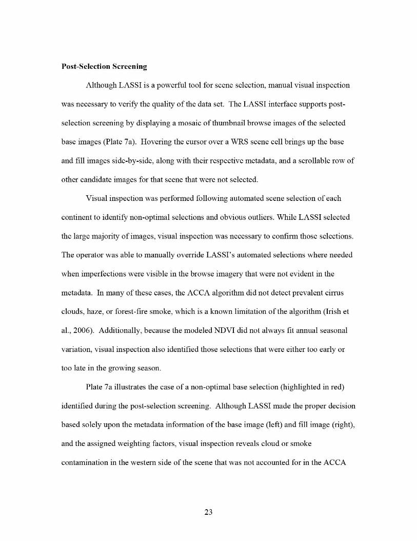
Post-Selection Screening
Although LASSI is a powerful tool for scene selection, manual visual inspection
was necessary to verify the quality of the data set. The LASSI interface supports post-
selection screening by displaying a mosaic of thumbnail browse images of the selected
base images (Plate 7a). Hovering the cursor over a WRS scene cell brings up the base
and fill images side-by-side, along with their respective metadata, and a scrollable row of
other candidate images for that scene that were not selected.
Visual inspection was performed following automated scene selection of each
continent to identify non-optimal selections and obvious outliers. While LASSI selected
the large majority of images, visual inspection was necessary to confirm those selections.
The operator was able to manually override LASSI's automated selections where needed
when imperfections were visible in the browse imagery that were not evident in the
metadata. In many of these cases, the ACCA algorithm did not detect prevalent cirrus
clouds, haze, or forest-fire smoke, which is a known limitation of the algorithm (Irish et
al., 2006). Additionally, because the modeled NDVI did not always fit annual seasonal
variation, visual inspection also identified those selections that were either too early or
too late in the growing season.
Plate 7a illustrates the case of a non-optimal base selection (highlighted in red)
identified during the post-selection screening. Although LASSI made the proper decision
based solely upon the metadata information of the base image (left) and fill image (right),
and the assigned weighting factors, visual inspection reveals cloud or smoke
contamination in the western side of the scene that was not accounted for in the ACCA
23

score (zero). The other candidate images, shown at the bottom of the screen, are all
either leaf-off winter images or have considerable cloud cover. Accepting that the
original pairing was the best selection, the operator elected to swap the base and fill
selections, using the slightly contaminated image as the fill instead of the base to yield a
better gap-filled composite product.
The post screening process also involved assessing image selections that appear to
be outliers in the metadata visualization maps. Plate 4 offers a good example of this.
The scene directly below Hudson Bay, Canada, looks suspicious because all of its
neighboring scenes have acceptable area coverage, but this one scene (in red) has an area
coverage of only 82.5 percent. Plate 7b presents a closer look at the chosen images and
the shallow pool of candidates for this scene. Three of the five candidates were winter
scenes with very low NDVI. Since NDVI was the most heavily weighted parameter,
LASSI chose the pair of images with higher NDVI, trading against low area coverage.
There were no other satisfactory choices. In this example, it was preferred to choose a
Landsat 7 ETM+ image pair with low area coverage but with a similar stage of growth,
than to have a pair with high area coverage but taken in incompatible seasons. In this case
LASSI selected the correct pair, and no manual adjustment to the selection was made.
24

(a)
{ WRS 033 / 021Fill Data 2007/133NDVIALCAArea
0.64093.2 e
GPS
WRS 033/021: 1 B candidate images
,Left-Bert . View ell candidates.<Right-BU n>: Popup menu.
.?1 y - HJ ,rp^} .^.
SensorWRSDateNDVIAC
L70 / 0232009/1630.8
.8 9
0
+Y=•pE®17
RR''^F[[44a
e
v
Sensor L7WRS 0271023I'll Date 2007/139NDVI 011ACCA 0
Are aGPS
82.5%0.25
'J'``
Area 82.5%GPS 0.11
r•//
WRS 027/023. G a ididate images
<Left-Buff— :View all candidates.< Right-Bulton>: Popup menu
Plate 7 (a) LASSI post-screening interface showing an example of non-optimal base-fill
assignment, where "flipping" the LASSI assignments would result in a better gap-filled product
and (b) LASSI post-screening interface showing a selection that had low area coverage. There
was no correction to the LASSI selection due to the lack of other leaf-on ima
25

At times, the operator had to choose between two very similar images. If the
modeled NDVI (based on the date of acquisition) of both images was similar, then they
were visually analyzed to detennine which one was in a higher stage of seasonal green-
up. If, after that examination, the decision was still not clear, the inspector would select
the one that was later in the season, especially in the northern regions of Canada and
Alaska where the growing season has a slow start due to ice melt-off in the spring.
Special cases and exceptions
Processing Landsat 7 images pairs is very common — almost 40 percent of all recent
Landsat 7 sales use multiple images. However, the processing of over 9,000 scenes for
GLS2005 has given an unprecedented view into the nuances of scene selection for SLC-
off image pairs. Areas of persistent clouds during the growing season proved extremely
problematic for scene selection, even given the depth of the U.S. archive. The scene
selection task for the North American continent provided many lessons learned. The
following sections discuss special cases and exemptions encountered during the selection
and subsequent screening processes.
Landsat 7 ETM+ bumper mode transition
On April 1, 2007, the Landsat 7 ETM+ instrument transitioned from Scan Angle Mirror
(SAM) mode to Bumper Mode. This change of operations occurred when the ETM+
scan mirror bumper wear exceeded the specifications for SAM mode operation. Bumper
mode resulted in an immediate, significant increased scan-time length, which made it
impossible to form a composite product from images taken in these two incompatible
26

modes. To avoid data processing problems, a rule was added to LASSI disallowing an
image collected prior to April 1, 2007 to be matched with an image collected after that
date.
Gap phase drift
Biophysically, images acquired more than two years apart could be matched as Landsat 7
pairs as long as they were seasonally consistent. However, after processing some of these
image pairs, the resulting composite product was consistently falling below the predicted
area coverage. As mentioned above, the scan mirror bumpers on the Landsat 7 ETM+
have worn in a linear pattern since launch. As the bumpers wore over time, the ETM+
mirror scan period lengthened. If images were acquired more than 16 months apart, there
was too great of an offset between images to process them to the predicted area coverage.
As a result, the Difference in Acquisition Date between pairs (difAD_P) parameter
should have been weighted much higher to preclude the matching of images from dates
that were too far apart. After learning this lesson, we enhanced LASSI to compute a more
precise estimate of area-coverage considering the age difference between a candidate pair
in the computation. Thereafter, LASSI's automated picks were considerably improved.
Only one Landsat 7 scene with ACCA <10 percent
The image pool from which LASSI made its selections was initially constrained to those
with ACCA scores of 10 or less. As a consequence, twelve scene locations in North
America only offered one ETM+ image in the pool, making image pairings impossible.
27

In this situation, we searched outside of LASSI, using one of the USGS's satellite
imagery search engines, such as G1oVis or EarthExplorer, to find the best matching
second image that was consistent with the selection criteria (other than ACCA). Because
the resulting image pairs exceeded the established cloud-cover thresholds-4 percent for
the base image, 8 percent for the fill image—they were not gap-filled, but rather provided
as multiple single image selections in the GLS2005 data set. We considered area
coverage and the other selection criteria during the search, so as not to preclude gap-
filling of these images by the end-user, if desired. We were able to find a pairing image
for all but 5 of the 12 locations, as shown in Plate 5.
No cloud free image
In even fewer cases, there were Landsat path/rows that had no data with less than 10
percent cloud cover. For these locations, manual selection of either Landsat 5 or Landsat
7 was performed to achieve as much cloud free area coverage as possible. However, in
this case, more than two images were chosen (base and two fill images) to obtain clear
coverage with Landsat 7 data. These selections were provided as single images, rather
than gap-filled.
Imperfect gap-filling result
Analysis of the gap-filled products for GLS2005 concluded that most were of good
quality—it was impossible, in most cases, to detect seams in the gap-filled radiometry.
However, there were a few scenes that, when gap-filled, showed "contamination" in the
base layer from the fill layer. We were aware of this problem when gap-filling images
28

with some cloud cover, but we found the situation also applied to scenes with snow, haze,
or smoke, none of which was called out in the metadata considered by LASSI. Many of
these occurrences were in northern Canada where only one image in a selected pair was
free of snow or ice. This also occurred in areas contaminated by smoke from large fires.
Since it was obvious that Landsat 7 gap-filled imagery would not be adequate, and there
were no Landsat 5 cloud-free candidates, we applied a three-tier strategy for accepting
other imagery:
1. Consider Landsat 5 imagery that had as little cloud cover as possible.
2. Relax the temporal requirement for Landsat 5 TM and Landsat 7 ETM+
imagery to allow imagery from as early as late-2003.
3. For high-latitude scenes, where there is substantial overlay from its easterly
and westerly neighbors, substitute acceptable imagery from east and west
adjacent paths when they entirely covered a problematic scene.
This approach was applied as a last resort when there was no acceptable choice of
imagery available. While this alternative strategy was needed in certain scenes, it was
only applied to less than 1 % of the North America selections as a consequence of the
deep archive of candidate imagery of this continent.
29

Coastal and non-continental land scenes
The LASSI tool is highly dependent on NDVI and cloud cover estimates. NDVI is often
not available for scenes with small islands. Additionally, cloud-cover estimates made on
a full-scene basis can be misleading in scenes where land is present in only a small part
of the scene, such as islands and coasts. For these reasons, islands were excluded from
LASSI's automated scene selection and were instead manually selected. Coastal scenes
selected by LASSI were visually inspected with extra scrutiny.
Conclusions
Using an automated approach (LASSI) to select the imagery for GLS2005 was an
advance over the three previous global surveys. With the increased complexity of
GLS2005 scene selection due to a multi-sensor approach, and challenges associated with
gap-filling requirements, scene selection without the use of a computer algorithm would
have been extremely labor intensive. Although using the LASSI tool dramatically eased
this complex process, human input and guidance was still necessary to set the parameter
weights, review the results, and manually intervene to override some selections.
Learning the tendencies of the algorithm in order to properly weight its selecting
parameters was an effort within itself and took time to set the weighting scheme to obtain
the "optimal" result for each continent or biome. There will be situations where users
would prefer a different image for their applications or studies, for example imagery that
is not at peak-greenness, but this is always a limitation of a single data set.
30

Overall, employing LASSI has enabled us to select a data set that is
phenologically superior to any other Global Land Survey. Previous GLS data sets were
conceived as single-sensor data sets (e.g. Landsat MSS for GLS 1975, Landsat 5 TM for
GLS 1990, and Landsat 7 ETM+ for GLS2000). By expanding the available data sources
to include Landsat 5 and 7, as well as ASTER and EO-1, the GLS2005 had a richer
selection of imagery to choose from. In addition, previous GLS data sets emphasized
cloud-free coverage, sometimes at the expense of obtaining leaf-on seasonality.
Consequently, for some regions (e.g. dry deciduous tropics) the GLS 1990 and GLS2000
data are not always useful for mapping land cover conditions. By fine tuning the
weighting criteria within LASSI we have successfully balanced seasonality with cloud-
clearing.
Acknowledgements
We would like to thank the NASA Land Cover Land Use Change (LCLUC) program for
their support in funding the work. We also thank Darrel Williams for added support
through the Landsat Project Science Office. This work could not be accomplished
without Dr. Robert A. Morris and Dr. Lina Khatib at the Computational Sciences
Division of NASA Ames Research Center for developing the Global Map Generator
(GMG) algorithm, which serves as the heart of LASSI. Lastly, we appreciate the
reviewers' constructive comments.
31

References
Gutman, G., R. Byrnes, J. Masek, S. Covington, S, C. Justice, S. Franks, and R. Headley,
2008. Towards monitoring land cover and land-use changes at a global scale: The
Global Land Survey 2005, Photogrannnetr •ic Engineering & Remote Sensing,
74(1).
Irish, R.R., J.L.Barker, S.N. Goward, and T. Arvidson, 2006. Characterization of the
Landsat 7 ETM+ Automated Cloud-Cover Assessment (ACCA) Algorithm,
Photogrammetric Engineering & Remote Sensing, 72(10):1179-1188.
James, M. E. and S. N. V. Kalluri, 1994. The Pathfinder AVHRR land data set: An
improved coarse resolution data set for terrestrial monitoring, International
Journal of Remote Sensing, Special Issue on Global Data Sets 15(17):3347-3363.
Khatib, L., J. Gasch, R. Morris, and S. Covington, 2007. Local Search for Optimal Global
Map Generation Using Mid-Decadal Landsat Images, Proceedings ofAAAI
Workshop on Preference Handlingfor A rtificial Intelligence, Vancouver, BC.
LPDAAC, 2001. MODIS/Terra Land Cover Types Yearly L3 Global 0.05Deg CMG
MOD12C1, URL: http://edcdaac.usgs.gov/modis/modl2clv4.asp, U.S.
Geological Survey (USGS) Center for Earth Resources Observation and Science
(EROS), Sioux Falls, South Dakota (last date accessed: 2 September 2008).
Masek, J.G., 2007. White Paper on Use of Gap-Filled Products for the Mid-Decadal
Global Land Survey (MDGLS), URL:
32

http://Icluc.umd.edu/mdgls/documents/MDGLS_gapfill.pdf (last date accessed: 2
September 2008).
Tucker, C.J., D. Grant and J. Dykstra, 2004. NASA's global orthorectified Landsat data
set, Photogrammetric Engineering & Remote Sensing, 70:313-322.
Williams, D.L., S. Goward, and T. Arvidson, 2006. Landsat: Yesterday, Today, and
Tomorrow, Photogrammetric Engineering & Remote Sensing, 72(10):1171-1178.
Yang, L., C. Homer, K. Hegge, C. Huang, B. Wylie, and B. Reed, 2001. A Landsat 7
Scene Selection Strategy for a National Land Cover Database, Proceedings of the
IEEE 2001 International Geoscience and Remote Sensing Symposium (Sydney,
Australia), unpaginated CD-ROM.
33


