
1
Abstract-- This paper presents a new method for studying
electromechanical transients in power systems using three phase,
combined transmission and distribution models (hybrid models).
The methodology models individual phases of an electric network
and associated unbalance in load and generation. Therefore, the
impacts of load unbalance, single phase distributed generation and
line impedance unbalance on electromechanical transients can be
studied without using electromagnetic transient simulation
(EMTP) programs. The implementation of this methodology in
software is called the Three Phase Dynamics Analyzer (TPDA).
Case studies included in the paper demonstrate the accuracy of
TPDA and its ability to simulate electromechanical transients in
hybrid models. TPDA has the potential for providing electric
utilities and power system planners with more accurate assessment
of system stability than traditional dynamic simulation software
that assume balanced network topology.
Index Terms— EMTP, Power System Stability, Distributed
Power Generation, Power Quality, Power System Restoration
I. INTRODUCTION
N recent years solar photovoltaic (hereafter referred to as PV)
based Distributed Generation (DG) has become very popular.
The reference case in the 2014 Annual Energy Outlook
released by the Energy Information Administration (EIA)
highlights this popularity, as it assumes that PV and wind will
continue to dominate the new commercial DG capacity and
account for 62.3% of the total commercial DG capacity in 2040,
thereby providing about 10% of the total electric energy
generated in the US [1]. However, the distribution of DG across
the nation is not going to be uniform. Some regions and utilities
will have more DG than others. For example, the state of
California is a leader in PV generation with the installed
capacity of rooftop solar PV at 2 GW in 2013 [2]. Utilities in
This is the accepted version (not the IEEE-published version) of the paper that has been accepted for publication in the IEEE Transactions on Power
Systems. The IEEE published version of the paper can be obtained from
ieeexplore.
Citation of the Published Version: H. Jain, A. Parchure, R. P. Broadwater, M.
Dilek and J. Woyak, "Three-Phase Dynamic Simulation of Power Systems Using Combined Transmission and Distribution System Models," in IEEE
Transactions on Power Systems, vol. 31, no. 6, pp. 4517-4524, Nov. 2016.
Digital Object Identifier (DOI) of the Published Version:
10.1109/TPWRS.2016.2535297
URL of the IEEE published article: http://ieeexplore.ieee.org/stamp/stamp.jsp?tp=&arnumber=7426417&isnumbe
r=7593404
regions with large numbers of DGs connected to their network
are already facing integration challenges, which are only going
to increase in the future. To effectively address the challenge of
integrating DG and ensuring the reliability of the electric grid,
planners and operators need new modeling and analysis tools
that can provide them with accurate information about the
impact of adding DG, and also to help them formulate strategies
to mitigate adverse impacts. With this objective in mind, we
present in this paper a new approach for studying
electromechanical transients in power systems using three
phase hybrid models to facilitate a more comprehensive
investigation of the impacts of adding DG in the electric grid.
The software implementation of this methodology is called the
Three Phase Dynamics Analyzer, or TPDA.
So far many authors have attempted to develop approaches
for studying the dynamics of distribution systems, particularly
under different penetration levels of DG. Many of these studies
have used balanced network representations of distribution
systems [3], [4] and/or small networks to test their approaches
[3]-[7]. The authors in [8] developed models for synchronous
DGs and Doubly Fed Induction Generators (DFIGs), and used
PSCAD/EMTPDC software to perform transient stability
studies on unbalanced networks with DGs. Authors in [9]
developed a method for performing three phase power flow
analysis on an unbalanced network and used the results of the
power flow to obtain an equivalent positive sequence network
that included contributions from the negative and zero sequence
networks. The equivalent positive sequence network was used
for performing dynamic simulations. It was not clear how the
authors could completely incorporate the impact of negative
and zero sequence networks in the equivalent positive sequence
network, since these networks cannot be decoupled under
general unbalance (unbalance at more than one location in an
As per section 8.1.9 of the IEEE PSPB Operations manual, the following copyright notice is being added here:
IEEE Copyright Notice: ©2016 IEEE. Personal use of this material is permitted. Permission from IEEE must be obtained for all other uses, in any
current or future media, including reprinting/republishing this material for
advertising or promotional purposes, creating new collective works, for resale or redistribution to servers or lists, or reuse of any copyrighted component of
this work in other works.
1Himanshu Jain, Abhineet Parchure and Robert Broadwater are with the
Electrical and Computer Engineering Department at Virginia Tech, Blacksburg,
VA 24061 (e-mail: [email protected];[email protected];[email protected]). 2 Murat Dilek and Jeremy Woyak are with Electrical Distribution Design
(EDD), Blacksburg, VA 24060,USA (e-mail: [email protected];
Himanshu Jain1, Abhineet Parchure1, Robert P. Broadwater1, Member, IEEE, Murat Dilek2, and
Jeremy Woyak2
Three-Phase Dynamic Simulation of Power
Systems Using Combined Transmission and
Distribution System Models
I
2
electric network). Authors in [10] studied the impact of DG on
the bulk transmission system, but used a balanced network for
their analysis. This paper was interesting because it highlighted
the need for studying the impacts of DG connected to the
distribution network on bulk transmission, sentiments echoed
by utility engineers as mentioned in a 2013 California Public
Utilities Commission report [11]. An interesting mathematical
model to study the small signal stability of unbalanced power
systems was presented in [12]. The work of the authors in [12]
was unique because, unlike in a balanced power system, a static
equilibrium point for linearization cannot be defined in
unbalanced systems. However, to develop the model the
authors assumed that the synchronous machine dynamics can
be “separated into its respective sequence components”. Since
the sequence components cannot be decoupled under general
unbalance in a network, we are of the view that more
experiments need to be conducted to identify the degree of
unbalance up to which the assumptions of the paper can be
justified.
Based on the above discussion it may be concluded that
studying electromechanical transients in unbalanced networks
is a difficult problem, and short of modeling the electric
network using differential equations in EMTP programs,
simplifying assumptions must be made to make the problem
tractable. Moreover, we did not come across a study that
simulated power system dynamics using hybrid models.
In light of these observations, this paper presents an
algorithm that enables the study of electromechanical transients
in unbalanced networks without using EMTP programs and
without assuming the network to be balanced, an assumption
commonly made in commercial electromechanical transient
simulation software.
II. CONCEPTS AND ALGORITHM BEHIND TPDA
Study of electromechanical transients in power systems
involves the formulation and solution of a set of Differential
Algebraic Equations (DAEs) [13], [14]. Commercial software
that are used for studying electromechanical transients, such as
GE-PSLF® and PTI-PSS/E®, assume the network to be
balanced. Under this assumption the solution of DAEs is
simplified because Park’s transformation enables direct
conversion from 𝑑𝑞0 frame voltages and currents in the time
domain to corresponding phasors in the frequency domain [13].
The DAEs formed using unbalanced three phase network
models, however, do not offer such simplification because six
unknown quantities (phasor magnitudes and angles of the three
phases) at an instant need to be estimated in the 𝑎𝑏𝑐 reference
frame from three instantaneous 𝑑𝑞0 reference frame quantities.
Discussion about a mathematically sound solution of this
problem is the primary focus of this section. This solution is
implemented in TPDA and distinguishes it from existing
electromechanical transient simulation software. Reference
[15] was the only reference found that presented a method for
obtaining the three phase phasors from 𝑑𝑞0 frame quantities.
However, the justification for the formula used was not
presented.
The discussion that follows assumes for simplicity that
synchronous generators are the only active devices in the
network that act as voltage sources. However, TPDA can
include any active device that can be modeled in three phase.
A. Calculation of Six 𝑑𝑞0 frame Voltages
The first step for obtaining three unique voltage phasors is
to calculate six 𝑑𝑞0 frame voltages. Generator stator algebraic
equations (1)-(3) are used to obtain these voltages. The
interested reader is referred to [13], [14] and Manuals of GE-
PSLF® and PTI-PSS/E® for a detailed discussion and derivation
of synchronous generator equations. Table I describes the
symbols used in (1)-(3).
𝑣𝑑 = −𝑅𝑠𝐼𝑑 −𝜔
𝜔𝑠𝜓𝑞 (1)
𝑣𝑞 = −𝑅𝑠𝐼𝑞 +𝜔
𝜔𝑠𝜓𝑑 (2)
𝑣0 = −𝑅𝑠𝐼0 (3)
TABLE I
Definition of Symbols Used in (1)-(3) Symbol Definition Symbol Definition
𝜓𝑑, 𝜓𝑞 𝑑, 𝑞 axis fluxes 𝜔𝑠 Synchronous Speed
(radians/second)
𝑣𝑑, 𝑣𝑞, 𝑣0 𝑑, 𝑞, 0 axis voltages 𝑅𝑠 Stator resistance
𝐼𝑑, 𝐼𝑞, 𝐼0 𝑑, 𝑞, 0 axis currents 𝜔 Rotor Speed (also a
dynamic state variable);
Before proceeding further it is important to mention that
similar to the commercial software that use balanced network
models for studying electromechanical transients, TPDA
assumes that the network frequency stays fixed at 60 Hz. For
studying electromechanical transients this assumption
introduces negligible error in the simulation results as system
frequency deviates little from 60 Hz [14]. This assumption,
along with the modeling of the electric network as algebraic
equations, allows network equations to be solved using a
nonlinear equations solver (e.g., a modified power flow analysis
program).
Calculation of six 𝑑𝑞0 frame voltages in TPDA at every
simulation iteration is now discussed. Let us assume that the
current simulation time instant is 𝑡 and the updated voltage
phasor is to be obtained for time 𝑡 + ∆𝑇. TPDA first solves the
network algebraic equations at time 𝑡 using the voltage phasors
at generator terminals 𝑉𝑎𝑒𝑗𝛽𝑎 , 𝑉𝑏𝑒𝑗𝛽𝑏 , 𝑉𝑐𝑒𝑗𝛽𝑐 to obtain new
current phasors 𝐼𝑎𝑒𝑗𝛾𝑎 , 𝐼𝑏𝑒𝑗𝛾𝑏 , 𝐼𝑐𝑒𝑗𝛾𝑐. These current phasors are
converted into instantaneous currents 𝑖𝑎(𝑡), 𝑖𝑏(𝑡), 𝑖𝑐(𝑡) using
(4)-(6). Park’s transform is used to calculate 𝑑𝑞0 frame currents
𝑰𝑑𝑞0(𝑡) from 𝒊𝑎𝑏𝑐(𝑡), where 𝒊𝑎𝑏𝑐(𝑡) = [𝑖𝑎(𝑡) 𝑖𝑏(𝑡) 𝑖𝑐(𝑡)]T
𝑖𝑎(𝑡) = √2𝐼𝑎 cos(2𝜋 ∗ 60 ∗ 𝑡 + 𝛾a) (4)
𝑖𝑏(𝑡) = √2𝐼𝑏 cos(2𝜋 ∗ 60 ∗ 𝑡 + 𝛾b) (5)
𝑖𝑐(𝑡) = √2𝐼𝑐 cos (2𝜋 ∗ 60 ∗ 𝑡 + 𝛾c) (6)
𝑰𝑑𝑞0(𝑡) is then used to solve the generator rotor differential
equations. However, instead of solving the differential
equations up to 𝑡 + ∆𝑇 as would be done in a conventional
dynamic simulator, TPDA solves the equations from 𝑡 to 𝑡 +∆𝑇 − 𝜖; 𝜖 ≪ ∆𝑇 (based on simulations run thus far, all 𝜖
values smaller than ∆𝑇/ 10 give similar results). Since ∆𝑇 is
already very small (a minimum value of 1/4th of a cycle is used
to capture rotor speed oscillations at twice the fundamental
frequency due to unbalance), negligible error is introduced in
the dynamic states of the generator rotor from the states
obtained if the integration step was 𝑡 + ∆𝑇.

3
Next, the new generator states along with 𝑰𝑑𝑞0(𝑡) are used
to calculate 𝜓𝑞(𝑡 + ∆𝑇 − 𝜖 ) and 𝜓𝑑(𝑡 + ∆𝑇 − 𝜖) [13] which
are substituted in (1)-(3) to obtain 𝐯𝒅𝒒𝟎(𝑡 + ∆𝑇 − 𝜖), the 3X1
vector of 𝑑𝑞0 frame voltages at time 𝑡 + ∆𝑇 − 𝜖. The first three
of the desired six 𝑑𝑞0 frame voltages are now available.
To obtain the remaining three 𝑑𝑞0 frame voltages,
𝒊𝑎𝑏𝑐(𝑡 + ∆𝑇 − 𝜖 ) is calculated using the current phasors
obtained at time 𝑡 since the current waveform does not change
between 𝑡 and 𝑡 + ∆𝑇. 𝒊𝑎𝑏𝑐(𝑡 + ∆𝑇 − 𝜖 ) is transformed into
𝑰𝑑𝑞0(𝑡 + ∆𝑇 − 𝜖 ) using Park’s transform and used along with
the generator states at 𝑡 + ∆𝑇 (same as the states at 𝑡 + ∆𝑇 − 𝜖)
to obtain 𝜓𝑞(𝑡 + ∆𝑇) and 𝜓𝑑(𝑡 + ∆𝑇), which when substituted
in (1)-(3) gives 𝐯𝑑𝑞0(𝑡 + ∆𝑇). Therefore, six 𝑑𝑞0 frame
voltages are now available to uniquely calculate the three 𝑎𝑏𝑐
frame voltage phasors at the generator terminal.
B. Calculation of Three Phase Voltage Phasors from Six 𝑑𝑞0
frame Voltages
Equation (7) shows the general relation between 𝑑𝑞0 and
𝑎𝑏𝑐 frame voltages [13].
𝐯𝑑𝑞0(𝑡) = 𝐏(𝑡) ∗ 𝐯𝑎𝑏𝑐(𝑡) (7)
where, 𝐏(𝑡) is the Park Transformation Matrix at time 𝑡 [13],
and 𝐯𝑎𝑏𝑐(𝑡) is the vector of 𝑎𝑏𝑐 frame voltages at time 𝑡.
Assuming that the voltage waveform does not change
between 𝑡1 = 𝑡 + ∆𝑇 − 𝜖 and 𝑡2 = 𝑡 + ∆𝑇, the relation
between the 𝑑𝑞0 and 𝑎𝑏𝑐 frame voltages at 𝑡1 and 𝑡2 is:
𝐯𝒅𝒒𝟎(𝑡1) = 𝐏(𝑡1) ∗ 𝐯𝑎𝑏𝑐(𝑡1) (8)
𝐯𝒅𝒒𝟎(𝑡2) = 𝐏(𝑡2) ∗ 𝐯𝑎𝑏𝑐(𝑡2) (9)
Since 𝐏(𝑡) is always invertible, (8) and (9) can be used to
calculate unique values of 𝐯𝑎𝑏𝑐(𝑡1) and 𝐯𝑎𝑏𝑐(𝑡2) using (10) and
(11), respectively.
𝐯𝑎𝑏𝑐(𝑡1) = 𝐏−𝟏(𝑡1) ∗ 𝐯𝑑𝑞0(𝑡1) (10)
𝐯𝑎𝑏𝑐(𝑡2) = 𝐏−𝟏(𝑡2) ∗ 𝐯𝑑𝑞0(𝑡2) (11)
Once the unique values of 𝐯𝑎𝑏𝑐(𝑡1) and 𝐯𝑎𝑏𝑐(𝑡2) are
obtained, the three voltage phasors can be calculated. The
derivation for obtaining the phasors is given below.
Let 𝑉𝑒𝑗𝜃 be the voltage phasor of phase A. Let 𝑥1 and 𝑥2 be
its instantaneous values at 𝑡1 and 𝑡2 which are equal to the first
elements of vectors 𝐯𝑎𝑏𝑐(𝑡1) and 𝐯𝑎𝑏𝑐(𝑡2), respectively.
In the time domain the voltage phasor can be expressed as a
cosine waveform such as the one in (12).
𝑥(𝑡) = √2𝑉𝑐𝑜𝑠(𝜔𝑠𝑡 + 𝜃) (12)
(12) can be expanded using the standard trigonometric
identity for the cosine of two angles into:
𝑥(𝑡) = √2𝑉𝑐𝑜𝑠(𝜔𝑠𝑡)cos (𝜃) − √2𝑉𝑠𝑖𝑛(𝜔𝑠𝑡)sin (𝜃) (13)
Denoting √2𝑉 cos(𝜃) by 𝐴 and −√2𝑉 sin(𝜃) by 𝐵, (13)
can be written as:
𝑥(𝑡) = 𝐴𝑐𝑜𝑠(𝜔𝑠𝑡) + 𝐵𝑠𝑖𝑛(𝜔𝑠𝑡) (14)
Since 𝑥1 and 𝑥2 are two samples of (14) at 𝑡1 and 𝑡2,
respectively, we obtain:
𝑥1 = 𝐴𝑐𝑜𝑠(𝜔𝑠𝑡1) + 𝐵𝑠𝑖𝑛(𝜔𝑠𝑡1) (15)
𝑥2 = 𝐴𝑐𝑜𝑠(𝜔𝑠𝑡2) + 𝐵𝑠𝑖𝑛(𝜔𝑠𝑡2) (16)
𝐴 and 𝐵 can be calculated from (15) and (16) using the
formula in (17) as long as 𝑡2 − 𝑡1 ≠𝑛𝜋
𝜔𝑠; 𝑛 ∈ ℤ≥0.
[𝐴𝐵
] =[
𝑠𝑖𝑛(𝜔𝑠𝑡2) −𝑠𝑖𝑛(𝜔𝑠𝑡1)
−𝑐𝑜𝑠(𝜔𝑠𝑡2) 𝑐𝑜𝑠(𝜔𝑠𝑡1)]
𝑠𝑖𝑛(𝜔𝑠(𝑡2−𝑡1))[𝑥1
𝑥2] (17)
√2𝑉𝑐𝑜𝑠(𝜃) =𝑥1𝑠𝑖𝑛(𝜔𝑠𝑡2)−𝑥2𝑠𝑖𝑛(𝜔𝑠𝑡1)
𝑠𝑖𝑛(𝜔𝑠(𝑡2−𝑡1)) (18)
√2𝑉𝑠𝑖𝑛(𝜃) =𝑥1𝑐𝑜𝑠(𝜔𝑠𝑡2)−𝑥2𝑐𝑜𝑠(𝜔𝑠𝑡1)
𝑠𝑖𝑛(𝜔𝑠(𝑡2−𝑡1)) (19)
The magnitude and phase angle of the voltage waveform can
be obtained from (18) and (19) using (20) and (21),
respectively.
𝑉 = (1
√2) √(18)2 + (19)2 (20)
𝜃 = 𝑎𝑡𝑎𝑛2((19), (18)) (21)
In TPDA, phase B and C voltage phasors at time 𝑡 + ∆𝑇
are also calculated by applying (18) - (21) to the 2nd and 3rd
elements of 𝐯𝑎𝑏𝑐(𝑡1) and 𝐯𝑎𝑏𝑐(𝑡2), respectively.
C. Algorithm used in TPDA to solve the DAEs
The algorithm for simulating electromechanical transients
that incorporates the formulation discussed above is presented
in the flowchart of Fig. 1; Table II defines the symbols used in
Fig. 1. The algorithm shows that TPDA uses a sequential or
partitioned method for solving the DAEs [13], [14]; the
differential equations are solved using the trapezoidal method
as implemented in the ode23t function of MATLAB while the
Distributed Engineering Workstation (DEW®) software [16] is
used to solve the algebraic equations. The four reasons for
selecting this approach are as follows:
1. Conceptual and implementation simplicity; algebraic and
differential equation solvers can be selected independently.
2. Differential equations can be solved in any order and in
parallel over multiple processors.
3. While any nonlinear equation solver can be used to solve the
network algebraic equations, TPDA uses DEW® because the
algorithm used in DEW® can be easily modified to split a
network into multiple radial sections which can be solved in
parallel across multiple processors, thereby significantly
reducing the simulation time.
4. DEW® has been used to model utility networks that contain
more than 3 million components (lines, switches, loads, etc.),
and the only limitation encountered has been the physical
memory of the machine. Therefore, using DEW to solve the
network algebraic equations provides TPDA the capability to
simulate electromechanical transients in very large networks.
III. VALIDATION OF TPDA & ITS APPLICATION FOR STUDYING
ELECTROMECHANICAL TRANSIENTS IN HYBRID MODELS
Validation of TPDA with the WECC 9 bus system was
performed in [17]. In this section of the paper three case studies
are discussed which are designed to achieve the following
objectives:
1. Demonstrate the accuracy of TPDA in simulating
electromechanical transients under balanced and unbalanced
network conditions by comparing simulation results with GE-
PSLF® and the Alternative Transients Program (ATP),
respectively (case studies 1 and 2).
2. Demonstrate the ability of TPDA to simulate
electromechanical transients in large, real utility, hybrid models
(case study 3).
3. Highlight the advantages of studying electromechanical
transients using hybrid models (case study 3).

4
The case studies are described in Tables III & IV. For case
studies 1 and 2, rotor speed deviation (rotor speed minus
synchronous speed) and terminal voltages obtained using
TPDA are compared with calculations from GE-PSLF® and
ATP. The following measures are used to present this
comparison:
1. Plots of trajectories: to provide a visual representation of the
accuracy of TPDA.
2. Correlation coefficients: to quantify degree of match in the
shape of the trajectories of the comparison variables.
3. Root Mean Square Errors (RMSEs): to quantify the degree
of match in actual value of the comparison variables.
Fig. 1. Flowchart of algorithm
TABLE II
Definition of Symbols Used in Flowchart of Fig. 1 Symbol Definition
𝑖; 𝑗 Counter for buses with dynamic models; counter for
simulation iterations
TOT_MC;
MAXITER
Constant representing total # of buses with dynamic
models; Constant representing total # of simulation iterations
∆𝑇; 𝜖 Integration time step; a small number<<∆𝑇
�̅�𝑎𝑏𝑐𝑖(𝑡); �̅�𝑎𝑏𝑐𝑖
(𝑡) Vectors of voltage and current phasor at bus 𝑖 at time 𝑡
𝐯𝑎𝑏𝑐𝑖(𝑡);𝐈𝑎𝑏𝑐𝑖
(𝑡) Instantaneous voltage and current vectors for bus 𝑖 at
time 𝑡
𝐯𝑑𝑞0𝑖(𝑡); 𝐈𝑑𝑞0𝑖
(𝑡) 𝑑𝑞0 frame voltage and current vectors for bus 𝑖 at time
𝑡
Flag Ensures that at each simulation iteration 𝐯𝒅𝒒𝟎𝑖
(𝑡 +
∆𝑇 − 𝜖) and 𝐯𝒅𝒒𝟎𝑖(𝑡 + ∆𝑇) are correctly calculated
𝐱𝑖𝑛𝑡𝑒𝑟𝑓𝑎𝑐𝑒𝑖(𝑡)
State vector of dynamic model (e.g. synchronous
generator) that directly connects at the 𝑖𝑡ℎ bus
TABLE III
Description of Case Studies
Case
Study
#
Network
Topology
(Table IV)
Dynamic
Models Disturbance
1 IEEE 39
Bus
Generator
(GENROU)
1,500 MW; 552 MVAR
balanced increase at Bus 4 (3X original load) *
2 IEEE 39
Bus Generator
(GENROU)
280 MW; 2,870 MVAR
increase on Phase A at Bus 12
(99X original load) *
3 Utility
Model
Generator
(GENROU);
Substation (Infinite Bus)
Phase A to ground fault at a 60 kV substation; 0.2 ohm fault
impedance
* For case studies 1&2 disturbance was initiated at 0.1 & removed at 0.3 second
TABLE IV
Description of Network Topology
Component Type IEEE 39 Bus Utility Model
2-Phase Lines/Cables 0 1,758
3-Phase Lines/Cables 34 7,472
1-Phase Transformers 0 2,655
3-Phase Transformers 12 1,410
Fixed Shunt Capacitors 0 62
Switched Shunt Capacitors 0 38
Breakers and Switches 0 7,526
Total Loads (3-Phase, 2-
Phase and 1-Phase) 19* 4,153**
Total Elements 65 25,074
* Only 3-Phase loads; Constant impedance load model is assumed
** ZIP model for load on each phase
Due to limited space, results are provided for selected buses
only. Buses are selected such that results from multiple
locations in the networks can be presented. The parameters of
dynamic models used in case studies 1 and 2 are given in [18].
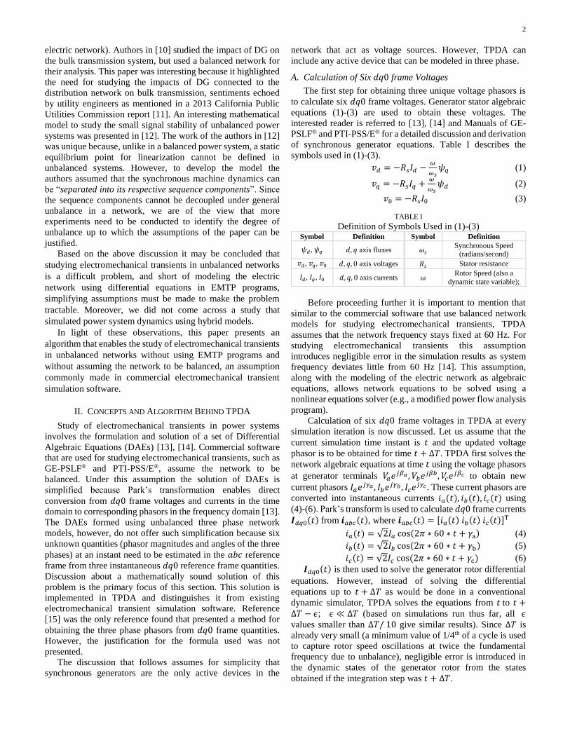
A. Case Study 1: Validation of TPDA with PSLF
The network topology used in case studies 1 and 2 is shown
in Fig. 2 [19]. The buses where disturbances were simulated and
for which results are provided in the figures and tables that
follow are indicated in Fig. 2.
Fig. 3 and 4 and Table V show that the trajectories generated
by PSLF and TPDA match very well and the RMSEs for all the
buses are very small while the correlation coefficients are close
to unity.
B. Case Study 2: Validation of TPDA with ATP
Similar to case study 1, rotor speed deviation and terminal
voltages calculated by TPDA and ATP match very well as seen
5
in Fig. 5 and 6. Moreover, Tables VI and VII show that the
RMSEs are small and correlation coefficients are close to 1.
Fig. 2. IEEE 39 bus system
Fig. 3. Case study 1: rotor speed deviation of generator at bus 30
Fig. 4. Case study 1: terminal voltage of generator at bus 31
Fig. 5. Case study 2: rotor speed deviation of generator at Bus 32
Fig. 6. Case study 2: three phase voltage at bus 12
TABLE V
Case Study 1: Correlation Coefficients and RMSE between
TPDA and PSLF
Generator
Bus #
Correlation Coefficients Root Mean Square Error
Rotor Speed
Terminal Voltage
Rotor Speed (Hz)
Terminal Voltage (p.u.)
30 0.97 0.99 0.002 0.0004
31 0.92 0.98 0.005 0.0026
32 0.96 0.94 0.006 0.0007
33 0.98 0.99 0.002 0.0003
34 0.99 0.81 0.002 0.0003
35 0.99 0.99 0.002 0.0004
36 0.98 0.95 0.002 0.0004
37 0.92 0.98 0.003 0.0004
38 0.97 0.96 0.002 0.0003
39 0.98 0.98 0.002 0.0003
TABLE VI
Case Study 2: Correlation Coefficients and RMSE of Rotor Speed
Deviation between TPDA and ATP
Generator
Bus #
Correlation
Coefficients
Root Mean Square Error
(Hz)
30 0.99 0.0003
31 0.98 0.0013
32 0.95 0.0015
33 0.98 0.0004
34 0.98 0.0005
35 0.99 0.0003
36 0.99 0.0003
37 0.98 0.0004
38 0.97 0.0007
39 0.99 0.0004
TABLE VII
Case Study 2: Correlation Coefficients and RMSE of Bus 12
Voltage between TPDA and ATP
Correlation
Coefficients
Root Mean Square Error
(p.u.)
Phase A 0.99 0.0227
Phase B 0.92 0.0042
Phase C 1.00 0.0011
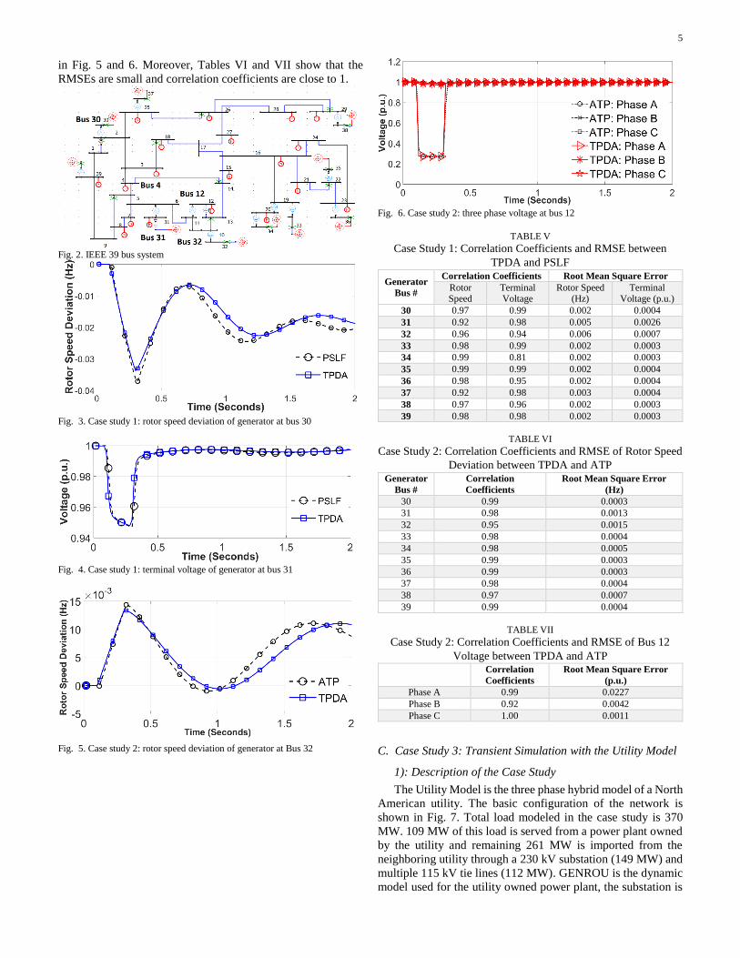
C. Case Study 3: Transient Simulation with the Utility Model
1): Description of the Case Study
The Utility Model is the three phase hybrid model of a North
American utility. The basic configuration of the network is
shown in Fig. 7. Total load modeled in the case study is 370
MW. 109 MW of this load is served from a power plant owned
by the utility and remaining 261 MW is imported from the
neighboring utility through a 230 kV substation (149 MW) and
multiple 115 kV tie lines (112 MW). GENROU is the dynamic
model used for the utility owned power plant, the substation is
6
modeled as an infinite bus, and the tie line flows are modeled
as constant power injections.
To highlight the advantages of using hybrid models, the case
study is simulated in two parts. First, the hybrid model with
detailed distribution feeder models is simulated. Next, the
“Transmission only Model (T-model)” is used in which all the
distribution feeders are de-energized and their loads are lumped
together at the corresponding 60 kV buses as constant power
loads. Fig. 8 shows the configuration of a substation in the
hybrid model (Fig. 8c) and the T-model (Fig 8a).
2): Description of Fault Simulation and Fault Clearing
For both the T- model and the hybrid model the single line
to ground (SLG) fault is assumed to occur on phase A of a 60
kV substation, just to the right of breaker B2 of Fig. 8a and Fig.
8c. This substation is serving 46 MW before the fault where
Feeder 1 (or S1) serves 14 MW (3% load imbalance) and Feeder
2 (or S2) serves 22 MW (0.3% load imbalance). The fault is
initiated at the end of the 50th cycle and cleared at the end of the
60th cycle by opening breakers B1 and B2 as shown in Fig. 8b
and 8d. Clearing the fault results in loss of power to load S2 in
the T-model (Fig. 8b) and Feeder 2 in the hybrid model (Fig.
8d). However, since the detailed substation configuration of the
12kV distribution network is included in the hybrid model, the
normally open breaker B3 is closed 30 cycles after the fault is
cleared to restore power to Feeder 2 (Fig. 8d).
Fig. 7. Configuration of the Utility Model
Fig. 8. Pre-fault, during fault and post-fault substation configuration
3): Important Observations from the Case Study
Simulation of electromechanical transients in hybrid
models using TPDA can provide utility engineers with insights
that cannot be obtained from transmission only models. Two
such insights were obtained from this case study – (i) the impact
of voltage sags on customers; and (ii) the ability of the network
to restore power to customers by reconfiguration. These are
discussed in detail below.
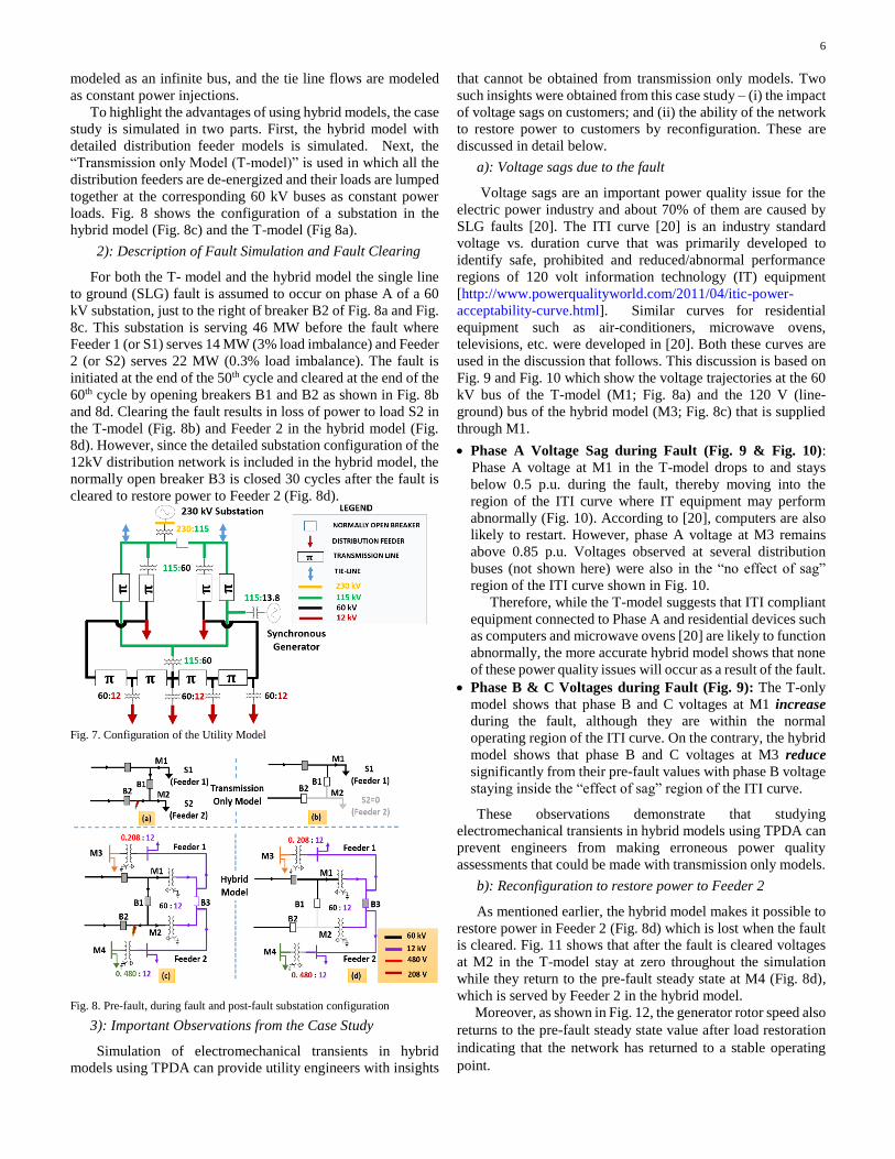
a): Voltage sags due to the fault
Voltage sags are an important power quality issue for the
electric power industry and about 70% of them are caused by
SLG faults [20]. The ITI curve [20] is an industry standard
voltage vs. duration curve that was primarily developed to
identify safe, prohibited and reduced/abnormal performance
regions of 120 volt information technology (IT) equipment
[http://www.powerqualityworld.com/2011/04/itic-power-
acceptability-curve.html]. Similar curves for residential
equipment such as air-conditioners, microwave ovens,
televisions, etc. were developed in [20]. Both these curves are
used in the discussion that follows. This discussion is based on
Fig. 9 and Fig. 10 which show the voltage trajectories at the 60
kV bus of the T-model (M1; Fig. 8a) and the 120 V (line-
ground) bus of the hybrid model (M3; Fig. 8c) that is supplied
through M1.
Phase A Voltage Sag during Fault (Fig. 9 & Fig. 10):
Phase A voltage at M1 in the T-model drops to and stays
below 0.5 p.u. during the fault, thereby moving into the
region of the ITI curve where IT equipment may perform
abnormally (Fig. 10). According to [20], computers are also
likely to restart. However, phase A voltage at M3 remains
above 0.85 p.u. Voltages observed at several distribution
buses (not shown here) were also in the “no effect of sag”
region of the ITI curve shown in Fig. 10.
Therefore, while the T-model suggests that ITI compliant
equipment connected to Phase A and residential devices such
as computers and microwave ovens [20] are likely to function
abnormally, the more accurate hybrid model shows that none
of these power quality issues will occur as a result of the fault.
Phase B & C Voltages during Fault (Fig. 9): The T-only
model shows that phase B and C voltages at M1 increase
during the fault, although they are within the normal
operating region of the ITI curve. On the contrary, the hybrid
model shows that phase B and C voltages at M3 reduce
significantly from their pre-fault values with phase B voltage
staying inside the “effect of sag” region of the ITI curve.
These observations demonstrate that studying
electromechanical transients in hybrid models using TPDA can
prevent engineers from making erroneous power quality
assessments that could be made with transmission only models.
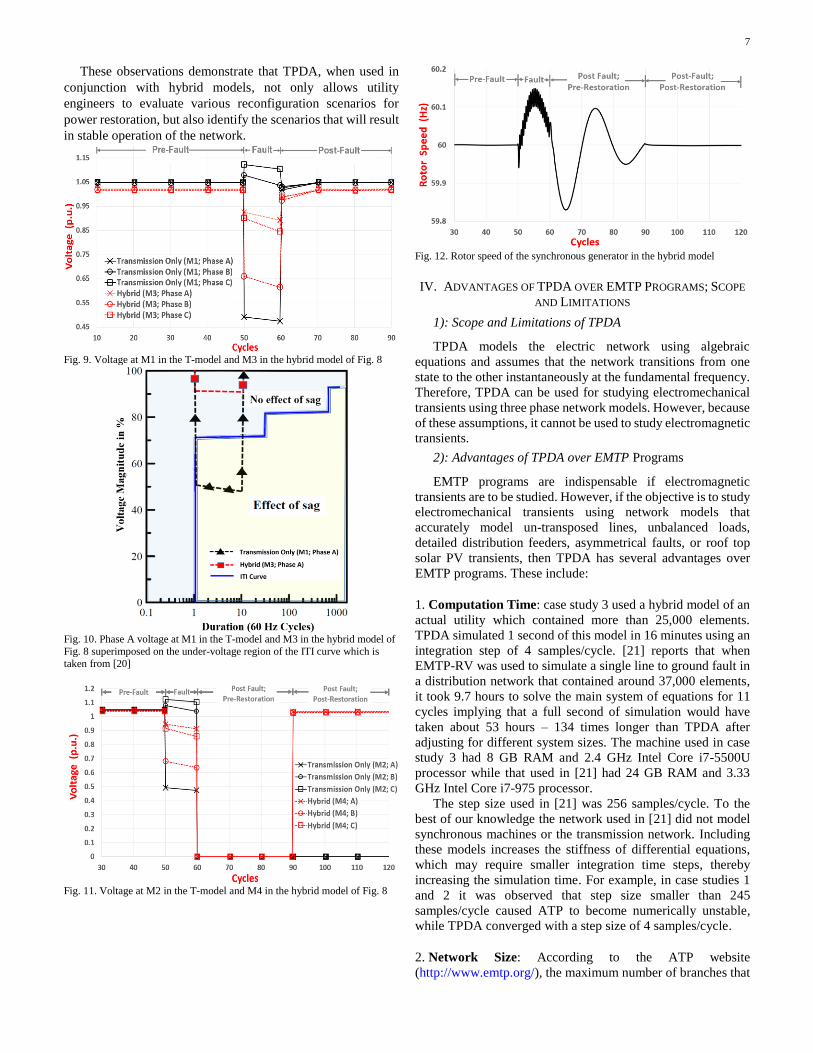
b): Reconfiguration to restore power to Feeder 2
As mentioned earlier, the hybrid model makes it possible to
restore power in Feeder 2 (Fig. 8d) which is lost when the fault
is cleared. Fig. 11 shows that after the fault is cleared voltages
at M2 in the T-model stay at zero throughout the simulation
while they return to the pre-fault steady state at M4 (Fig. 8d),
which is served by Feeder 2 in the hybrid model.
Moreover, as shown in Fig. 12, the generator rotor speed also
returns to the pre-fault steady state value after load restoration
indicating that the network has returned to a stable operating
point.
7
These observations demonstrate that TPDA, when used in
conjunction with hybrid models, not only allows utility
engineers to evaluate various reconfiguration scenarios for
power restoration, but also identify the scenarios that will result
in stable operation of the network.
Fig. 9. Voltage at M1 in the T-model and M3 in the hybrid model of Fig. 8
Fig. 10. Phase A voltage at M1 in the T-model and M3 in the hybrid model of
Fig. 8 superimposed on the under-voltage region of the ITI curve which is
taken from [20]
Fig. 11. Voltage at M2 in the T-model and M4 in the hybrid model of Fig. 8
Fig. 12. Rotor speed of the synchronous generator in the hybrid model
IV. ADVANTAGES OF TPDA OVER EMTP PROGRAMS; SCOPE
AND LIMITATIONS
1): Scope and Limitations of TPDA
TPDA models the electric network using algebraic
equations and assumes that the network transitions from one
state to the other instantaneously at the fundamental frequency.
Therefore, TPDA can be used for studying electromechanical
transients using three phase network models. However, because
of these assumptions, it cannot be used to study electromagnetic
transients.
2): Advantages of TPDA over EMTP Programs
EMTP programs are indispensable if electromagnetic
transients are to be studied. However, if the objective is to study
electromechanical transients using network models that
accurately model un-transposed lines, unbalanced loads,
detailed distribution feeders, asymmetrical faults, or roof top
solar PV transients, then TPDA has several advantages over
EMTP programs. These include:
1. Computation Time: case study 3 used a hybrid model of an
actual utility which contained more than 25,000 elements.
TPDA simulated 1 second of this model in 16 minutes using an
integration step of 4 samples/cycle. [21] reports that when
EMTP-RV was used to simulate a single line to ground fault in
a distribution network that contained around 37,000 elements,
it took 9.7 hours to solve the main system of equations for 11
cycles implying that a full second of simulation would have
taken about 53 hours – 134 times longer than TPDA after
adjusting for different system sizes. The machine used in case
study 3 had 8 GB RAM and 2.4 GHz Intel Core i7-5500U
processor while that used in [21] had 24 GB RAM and 3.33
GHz Intel Core i7-975 processor.
The step size used in [21] was 256 samples/cycle. To the
best of our knowledge the network used in [21] did not model
synchronous machines or the transmission network. Including
these models increases the stiffness of differential equations,
which may require smaller integration time steps, thereby
increasing the simulation time. For example, in case studies 1
and 2 it was observed that step size smaller than 245
samples/cycle caused ATP to become numerically unstable,
while TPDA converged with a step size of 4 samples/cycle.
2. Network Size: According to the ATP website
(http://www.emtp.org/), the maximum number of branches that
8
can be modeled in the standard EEUG program distribution is
10,000. As shown in Table IV, the Utility Model of case study
3 contains over 13,000 branches. Similarly, the maximum
number of switches that can be included in ATP are 1200, while
TPDA models 7,526 switches and breakers in case study 3.
Since TPDA uses DEW® for solving the algebraic
equations, system size is not a limitation. Actual utility
networks with more than 3 million components have been
modeled in DEW® on 32 bit desktop machines.
3. Convenient and Economic Deployment: TPDA uses the
same network models that are used by steady state analysis
applications in DEW®. Therefore, additional expenditure and
inconvenience of deploying and maintaining a separate EMTP
program and migrating data and models is avoided.
V. CONCLUSION
This paper introduces a new method and software tool,
TPDA, for studying electromechanical transients using three
phase network models. Through three case studies it is shown
that TPDA can accurately simulate electromechanical
transients under balanced and unbalanced network conditions,
and reveals useful engineering information from the simulation
of hybrid models that cannot be obtained from transmission
only models.
Our next objective is to use TPDA to study the impact of
DG, particularly solar PV, on the stability of power systems
using hybrid models of utilities. We are working on developing
the three phase and single phase DG dynamic models that are
needed for the study. We hope to share the results of this effort
with the power systems community in the near future.
VI. ACKNOWLEDGMENT
The authors gratefully acknowledge the guidance provided
by Dr. Steve Southward at Virginia Tech during the
development of the methodology discussed in this paper.
VII. REFERENCES
[1] U.S. Energy Information Administration, "Energy Outlook 2014," U.S. Department of Energy, Washington, DC, DOE/EIA-0383(2014), Apr.
2014. [Online]. Available: http://www.eia.gov/forecasts/archive/aeo14/
pdf/0383(2014).pdf [2] K. Kroh, “California Installed More Rooftop Solar in 2013 Than Previous
30 Years Combined”, Think Progress, Jan. 2014. [Online]. Available:
http://thinkprogress.org/climate/2014/01/02/3110731/california-rooftop-solar-2013/
[3] I. Xyngi, A. Ischenko, M. Popov, and L. Sluis, "Transient Stability
Analysis of a Distribution Network with Distributed Generators," IEEE Trans. Power Systems, vol. 24, pp. 1102-1104, May 2009.
[4] R.S. Thallam, S. Suryanarayanan, G.T. Heydt, and R. Ayyanar, "Impact
of Interconnection of Distributed Generation on Electric Distribution Systems – A Dynamic Simulation Perspective,” in Proc. 2006 IEEE
Power Engineering Society General Meeting.
[5] Z. Miao, M.A. Choudhry, and R.L. Klein, "Dynamic simulation and stability control of three-phase power distribution system with distributed
generators," in Proc. 2002 IEEE Power Engineering Society Winter
Meeting, pp.1029 – 1035. [6] B.W. Lee and S.B. Rhee, "Test Requirements and Performance
Evaluation for Both Resistive and Inductive Superconducting Fault Current Limiters for 22.9 kV Electric Distribution Network in Korea,"
IEEE Trans. Applied Superconductivity, vol. 20, pp. 1114-1117, June
2010.
[7] E.N. Azadani, C. Canizares, C and K. Bhattacharya, "Modeling and
stability analysis of distributed generation," in Proc. 2002 IEEE Power and Energy Society General Meeting.
[8] E. Nasr-Azadani, C.A. Canizares, D.E. Olivares, and K. Bhattacharya,
"Stability Analysis of Unbalanced Distribution Systems With Synchronous Machine and DFIG Based Distributed Generators," IEEE
Trans. Smart Grid, vol.5, pp. 2326-2338, Sept. 2014.
[9] Xuefeng Bai, Tong Jiang, Zhizhong Guo, Zheng Yan and Yixin Ni, "A unified approach for processing unbalanced conditions in transient
stability calculations," IEEE Trans. Power Systems, vol.21, pp. 85-90,
Feb. 2006. [10] M. Reza, J.G. Slootweg, P.H. Schavemaker, W.L. Kling, L van der Sluis.,
"Investigating impacts of distributed generation on transmission system
stability," in Proc. 2003 IEEE Bologna Power Tech Conference. [11] Black & Veatch, "Biennial Report on Impacts of Distributed Generation,"
California Public Utilities Commission, B&V Project No. - 176365, May
2013. [Online]. Available: http://www.cpuc.ca.gov/NR/rdonlyres/BE24C491-6B27-400C-A174-85F9B67F8C9B/0
/CPUCDGImpactReportFinal2013_05_23.pdf
[12] R.H. Salim and R.A. Ramos, "A Model-Based Approach for Small-Signal Stability Assessment of Unbalanced Power Systems," IEEE Trans. Power
Systems, vol.27, pp.2006-2014, Nov. 2012.
[13] P.W. Sauer and M.A. Pai, Power System Dynamics and Stability, Illinois:
Stipes Publishing L.L.C, 2006, p. 26, 35, 47, 155, 165, 195.
[14] P. Kundur, Power System Stability and Control, New Delhi: Tata
McGraw Hill, 2012, p. 858, 861. [15] S. Abhyankar, "Development of an Implicitly Coupled Electromechanical
and Electromagnetic Transients Simulator for Power Systems," Ph.D. dissertation, Dept. Elect. Eng., Illinois Institute of Technology, Chicago,
2011.
[16] M. Dilek, F. de Leon, R. Broadwater, and S. Lee, “A Robust Multiphase Power Flow for General Distribution Networks”, IEEE Trans. Power
Systems, vol. 25, pp. 760-768, May 2010.
[17] H. Jain, A. Parchure, R.P. Broadwater, M. Dilek, J. Woyak., "Three Phase Dynamics Analyzer - A New Program for Dynamic Simulation using
Three Phase Models of Power Systems," in Proc. 2015 IEEE IAS Joint
ICPS/PCIC Conference. [18] Parameters for Dynamic Models of Power Plant Equipment. [Online].
Available: https://www.scribd.com/doc/283485862/Parameters-for-
Dynamic-Models-of-Power-Plant-Equipment [19] IEEE 39 Bus System, Illinois Center for a Smarter Electric Grid
(ICSEG). [Online]. Available:
http://publish.illinois.edu/smartergrid/ieee-39-bus-system/ [20] G.G. Karady, S. Saksena, B. Shi, N. Senroy, "Effects of Voltage Sags on
Loads in a Distribution System," Power Systems Energy Research Center,
Ithaca, NY, PSERC Publication 05-63, Oct. 2005. [21] V. Spitsa, R. Salcedo, Ran Xuanchang, J.F. Martinez, R.E. Uosef, F. de
Leon, D. Czarkowski and Z. Zabar, "Three–Phase Time–Domain
Simulation of Very Large Distribution Networks," IEEE Trans. Power Delivery, vol.27, pp.677-687, April 2012.
VIII. BIOGRAPHIES
Himanshu Jain is pursuing his PhD in Electrical Engineering at Virginia Tech.
He holds a MS degree in Electrical Engineering from the University of Texas at Arlington and a B.Tech degree in Electrical Engineering from G.B. Pant
University of Agriculture and Technology. His research interests include power
system dynamics, renewable integration, and electricity markets.
Abhineet Parchure is currently pursuing his MS in Electrical Engineering at
Virginia Tech. He received a B.E. (Hons.) degree in Electrcal and Electronics Engineering from Birla Institute of Technology & Science, Pilani in 2012. His
research interests include renewable energy integration, power system
dyanmics and voltage stability of transmission and distribution systems.
Robert P. Broadwater (M’71) received the B.S., M.S., and Ph.D. degrees in
electrical engineering from Virginia Polytechnic Institute and State University
(Virginia Tech), Blacksburg, VA, in 1971, 1974, and 1977, respectively. He is currently a Professor of electrical engineering at Virginia Tech. He develops
software for analysis, design, operation, and real-time control of physical
systems. His research interests are object-oriented analysis and design and computer-aided engineering.
Murat Dilek received the M.S. and Ph.D. degrees in electrical engineering from Virginia Tech, Blacksburg, in 1996 and 2001, respectively. He is a Senior

9
Development Engineer at Electrical Distribution Design, Inc. His work
involves computer-aided design and analysis of electrical power systems.
Jeremy Woyak (S’07) received a B.S. degree in electrical engineering from
Lawrence Technological University, Southfield, MI, in 2010 and a M.S. degree in electrical engineering from Virginia Polytechnic Institute and State
University, Blacksburg, VA, in 2012. He is currently a software developer at
Electrical Distribution Design. He develops software for analysis, design, operation, and real-time control of electrical power systems.


