
General rights Copyright and moral rights for the publications made accessible in the public portal are retained by the authors and/or other copyright owners and it is a condition of accessing publications that users recognise and abide by the legal requirements associated with these rights.
• Users may download and print one copy of any publication from the public portal for the purpose of private study or research. • You may not further distribute the material or use it for any profit-making activity or commercial gain • You may freely distribute the URL identifying the publication in the public portal
If you believe that this document breaches copyright please contact us providing details, and we will remove access to the work immediately and investigate your claim.
Downloaded from orbit.dtu.dk on: Jun 06, 2018
Theoretical and Experimental Analysis of Adsorption in Surface-based Biosensors
Hansen, Rasmus; Hassager, Ole; Callisen, Thomas H,; Bruus, Henrik
Publication date:2012
Link back to DTU Orbit
Citation (APA):Hansen, R., Hassager, O., Callisen, T. H., & Bruus, H. (2012). Theoretical and Experimental Analysis ofAdsorption in Surface-based Biosensors. Technical University of Denmark, Department of ChemicalEngineering.

Rasmus HansenPh.D. ThesisJanuary 2012
Theoretical and Experimental Analysis of Adsorption in Surface-based Biosensors

Theoretical and ExperimentalAnalysis of Adsorption inSurface-based Biosensors
Rasmus Hansen
Department of Chemical and Biochemical Engineering
Technical University of Denmark
A thesis submitted for the degree of
Philosophiae Doctor (Ph.D.)
2012 January
1
Title of the thesis:Theoretical and Experimental Analysis of Adsorption in Surface-basedBiosensors
Author:Rasmus HansenE-mail: [email protected]
Supervisors:Ole Hassager, Professor, DTU Chemical EngineeringE-mail: [email protected]
Thomas H. Callisen, Senior Manager, Novozymes A/SE-mail: [email protected]
Henrik Bruus, Professor, DTU NanotechE-mail: [email protected]
Address:Department of Chemical and Biochemical EngineeringDanish Polymer CenterTechnical University of DenmarkSøltofts Plads, Building 227DK-2800 Kongens Lyngby, Denmark
Copyright c© 2011 Rasmus HansenAll rights reserved
ISBN 978-87-92481-75-7
Print:Jog R Frydenberg København august 2012
2

Preface
This thesis is submitted in partial fulfillment of the requirements for obtainingthe Ph.D. degree in chemical engineering at the Technical University of Denmark(DTU). The Ph.D. project was carried out partially at the Department of Chem-ical and Biochemical Engineering at DTU, and partially at Novozymes A/S, inthe period January 1st 2009 - January 13st 2012.
I would like to express my gratitude to my three supervisors for their supportduring the project. Thanks to Lene Bjørg Cesar and Diane Falk Rasmussen atNovozymes for their careful laboratory assistance. Thanks also to my colleaguesat the Danish Polymer Centre at DTU, especially Yanwei Wang with whom Ihave had many interesting hours, and Anders Egede Daugaard for encouragingconversations. I am also thankful to Stig Wedel at DTU Chemical Engineeringfor discussions on mathematical issues. I finally wish to thank my wife for indis-pensable support and indulgence during the project period.
The Ph.D. project has been funded by the The Danish Council for Indepen-dent Research - Technology and Production Sciences and by Novozymes A/S.
Kongens Lyngby, March 13st 2012.
Rasmus Hansen
i
3

4

Resume (in Danish)
Teoretisk og eksperimentel analyse af adsorption
i overfladebaserede biosensorer
Denne Ph.D. afhandling vedrører anvendelse af overflade-plasmon-resonans (SPR)spektroskopi, som er en overfladebaseret biosensorteknologi, til studier af ad-sorptionsdynamik. Afhandlingen indeholder eksperimentelt og teoretisk arbejde.I den teoretiske del udvikles teorien for konvektion, diffusion, og adsorption ioverfladebaserede biosensorer generelt. Vi studerer transportdynamikken i enmodelgeometri af en Biacore SPR sensor. Vi præsenterer en gennemgang samten analytisk løsning til en approksimativ kvasi-stationær teori, som bliver tagethyppigt i brug i SPR litteraturen for at indfange konvektiv og diffusiv masse-transport. Det dimensionsløse Damkohler tal, som naturligt parameteriserer denkvasi-stationære teori, udledes i termer af den dimensionsløse adsorptionskon-stant (Biot tallet), den dimensionsløse strømningshastighed (Peclet tallet), samtmodelgeometrien. Derudover udvikles og præsenteres en teoretisk to-komponentmodel, som er designet til at indfange kompetitiv adsorptionsdynamik af to slagsadsorberende specier. Vi foretager en numerisk undersøgelse af transient dy-namik, hvor vi kvantificerer fejlen ved at bruge den kvasi-stationære teori tileksperimentel datafitting, i bade det kinetisk begrænsede og det konvektions-diffusions-begrænsede regime. Resultaterne tydeliggør, under hvilke betingelserden kvasi-stationære teori er palidelig, og hvor den ikke er. Foruden det velk-endte faktum at gyldighedsintervallet for teorien er begrænset under konvektions-diffusions-begrænsede betingelser, vises det, hvorledes forholdet imellem indløbs-koncentrationen og den maksimale overfladekapacitet er kritisk for palidelig brugaf den kvasi-stationære teori. Vores teoretiske resultater tilvejebringer brugereaf overfladebaserede biosensorer et væktøj til at korrigere adsorptionskonstan-ter opnaet ved at fitte den kvasi-stationære teori til eksperimenter. Endelig un-dersøges konsekvensen af adsorption pa alle overfladerne, udover sensoroverfladen,i biosensorens flowcelle. I den del af afhandlingen der vedrører eksperimentelt ar-bejde bruger vi en Biacore SPR sensor til at studere adsorption af lipaser pa
iii
5

modeloverflader der imiterer substrat, samt at studere kompetitiv adsorption aflipase og overfladeaktive molekyler (surfactant). En del af den eksperimentelledata malt under projektperioden præsenteres og diskuteres. Denne del tilveje-bringer tilsyneladende kinetiske adsorptions- og desorptionkonstanter, og forsøgerat give et overblik over de vigtigste elementer der udfordrer brugen af den eksper-imentelle data til datadrevet teoretisk modellering. Vi fremhæver nogle vigtigebetingelser som skal være opfyldt for at opna en udførlig forbindelse mellemeksperimental data og teoretisk modellering.
iv
6
Abstract
The present Ph.D. dissertation concerns the application of surface plasmon reso-nance (SPR) spectroscopy, which is a surface-based biosensor technology, for stud-ies of adsorption dynamics. The thesis contains both experimental and theoreticalwork. In the theoretical part we develop the theory for convection, diffusion, andadsorption in surface-based biosensors in general. In particular, we study thetransport dynamics in a model geometry of a Biacore SPR sensor. An approxi-mate quasi-steady theory, which has been widely adopted in the SPR literatureto capture convective and diffusive mass transport, is reviewed, and an analyticalsolution is provided. The important nondimensional Damkohler number, inherentin the quasi-steady theory, is derived in terms of the nondimensional adsorptioncoefficient (Biot number), the nondimensional flow rate (Peclet number), and themodel geometry. Also, a two-component theoretical model, designed to capturecompetitive adsorption dynamics of two adsorbing species, is developed and pre-sented. Transient dynamics is investigated numerically, and we quantify the errorof using the quasi-steady theory for experimental data fitting in both kineticallylimited and convection-diffusion-limited regimes. The results clarify the condi-tions under which the quasi-steady theory is reliable or not. In extension to thewell known fact that the range of validity is limited under convection-diffusion-limited conditions, we also show how the ratio of the inlet concentration to themaximum surface capacity is critical for reliable use of the quasi-steady theory.Our theoretical results provide users of surface-based biosensors with a tool ofcorrecting experimentally obtained adsorption rate constants, based on the quasi-steady theory. Finally, the consequence of adsorption on all surfaces present inthe flow cell of the surface-based biosensor, in addition to the sensor surface, isinvestigated. In the experimental part of the thesis we use a Biacore SPR sensorto study lipase adsorption on model substrate surfaces, as well as competitiveadsorption of lipase and surfactants. A part of the experimental data obtainedduring the project is presented and discussed. In particular, this part providesapparent kinetic adsorption/desorption rate constants, and gives an overview ofthe major challenges of basing theoretical modeling on this data. We emphasizethe importance of some conditions, which necessarily have to be fulfilled in order
v
7
to attain a comprehensive link between the experimental data and the theoreticalmodeling.
vi
8
Contents
Preface i
Resume iii
Abstract v
List of Figures x
1 Introduction 11.1 Outline of the Ph.D. project . . . . . . . . . . . . . . . . . . . . . 11.2 Dissertation structure . . . . . . . . . . . . . . . . . . . . . . . . . 21.3 Publications . . . . . . . . . . . . . . . . . . . . . . . . . . . . . . 3
2 Introduction to SPR spectroscopy 52.1 The overall principle of SPR . . . . . . . . . . . . . . . . . . . . . 52.2 The optical reader . . . . . . . . . . . . . . . . . . . . . . . . . . 62.3 The sample preparation and delivery system . . . . . . . . . . . . 82.4 The biorecognition element . . . . . . . . . . . . . . . . . . . . . . 92.5 Analysis of interactions at lipid surfaces by use of SPR spectroscopy 92.6 SPR in the present thesis . . . . . . . . . . . . . . . . . . . . . . . 11
3 Mathematical modeling of transport phenomena in surface-basedbiosensors 133.1 System geometry and two-dimensional approximation . . . . . . . 143.2 Evolution equations . . . . . . . . . . . . . . . . . . . . . . . . . . 143.3 Unimolecular systems . . . . . . . . . . . . . . . . . . . . . . . . . 16
3.3.1 Surface adsorption kinetics . . . . . . . . . . . . . . . . . . 163.3.2 Nondimensional parameterization . . . . . . . . . . . . . . 173.3.3 Estimates of nondimensional parameters . . . . . . . . . . 193.3.4 The weak formulation . . . . . . . . . . . . . . . . . . . . 20
3.4 Bimolecular systems . . . . . . . . . . . . . . . . . . . . . . . . . 213.4.1 Surface adsorption kinetics . . . . . . . . . . . . . . . . . . 22
vii
9

CONTENTS
3.4.2 Nondimensional parameterization . . . . . . . . . . . . . . 253.4.3 Estimates of nondimensional parameters . . . . . . . . . . 27
3.5 The quasi-steady theory . . . . . . . . . . . . . . . . . . . . . . . 273.5.1 Correspondence between the Damkohler, Biot, and Peclet
number . . . . . . . . . . . . . . . . . . . . . . . . . . . . 303.5.2 Analytical solution of the quasi-steady theory . . . . . . . 313.5.3 Note on two-compartment model . . . . . . . . . . . . . . 31
4 Numerical Analysis 334.1 Numerical method . . . . . . . . . . . . . . . . . . . . . . . . . . 334.2 Evolution of the concentration fields . . . . . . . . . . . . . . . . . 344.3 Transient transport in surface-based biosensors . . . . . . . . . . . 37
4.3.1 Kinetic scaling . . . . . . . . . . . . . . . . . . . . . . . . 384.3.2 Diffusion scaling . . . . . . . . . . . . . . . . . . . . . . . 404.3.3 Flow rate dependency . . . . . . . . . . . . . . . . . . . . 424.3.4 Error of the quasi-steady theory . . . . . . . . . . . . . . . 424.3.5 Effect of preadsorption . . . . . . . . . . . . . . . . . . . . 444.3.6 Summary of results . . . . . . . . . . . . . . . . . . . . . . 45
5 SPR experiments of lipase adsorption 475.1 Introduction . . . . . . . . . . . . . . . . . . . . . . . . . . . . . . 475.2 Materials and methods . . . . . . . . . . . . . . . . . . . . . . . . 50
5.2.1 Lipases and solvent . . . . . . . . . . . . . . . . . . . . . . 505.2.2 Surfactant . . . . . . . . . . . . . . . . . . . . . . . . . . . 505.2.3 Experimental protocol . . . . . . . . . . . . . . . . . . . . 50
5.3 Adsorption of lipase on hydrophobic surfaces . . . . . . . . . . . . 505.3.1 Presentation and discussion of data . . . . . . . . . . . . . 515.3.2 Inconsistency with expected behavior . . . . . . . . . . . . 525.3.3 Head to head comparison of wild type and mutant lipase . 545.3.4 Lipase adsorption rate constants . . . . . . . . . . . . . . . 55
5.4 Competitive adsorption of lipase and surfactant . . . . . . . . . . 565.4.1 Identification of competitive regime . . . . . . . . . . . . . 565.4.2 The competitive adsorption dynamics of lipase and surfactant 585.4.3 Surfactant dynamics from Langmuir adsorption model . . 605.4.4 Lipase adsorption rate constants . . . . . . . . . . . . . . . 625.4.5 Problems with reproducibility . . . . . . . . . . . . . . . . 63
6 Concluding remarks 656.1 Conclusions . . . . . . . . . . . . . . . . . . . . . . . . . . . . . . 656.2 Future perspective . . . . . . . . . . . . . . . . . . . . . . . . . . 66
6.2.1 Future theoretical work . . . . . . . . . . . . . . . . . . . . 66
viii
10

CONTENTS
6.2.2 Future experimental work . . . . . . . . . . . . . . . . . . 666.2.3 Future work in the interface between theory and experiments 67
References 69
ix
11
List of Figures
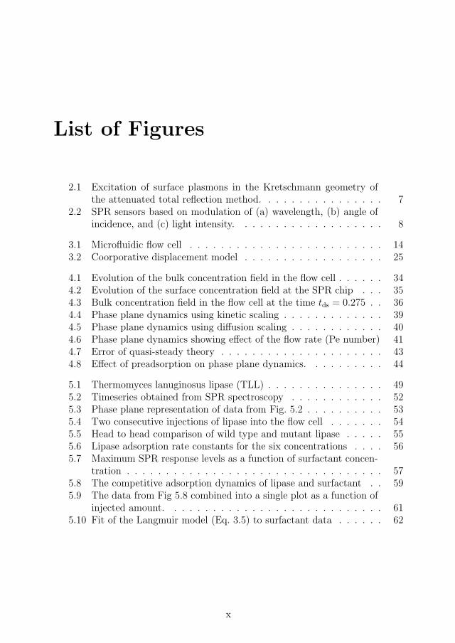
2.1 Excitation of surface plasmons in the Kretschmann geometry ofthe attenuated total reflection method. . . . . . . . . . . . . . . . 7
2.2 SPR sensors based on modulation of (a) wavelength, (b) angle ofincidence, and (c) light intensity. . . . . . . . . . . . . . . . . . . 8
3.1 Microfluidic flow cell . . . . . . . . . . . . . . . . . . . . . . . . . 143.2 Coorporative displacement model . . . . . . . . . . . . . . . . . . 25
4.1 Evolution of the bulk concentration field in the flow cell . . . . . . 344.2 Evolution of the surface concentration field at the SPR chip . . . 354.3 Bulk concentration field in the flow cell at the time tds = 0.275 . . 364.4 Phase plane dynamics using kinetic scaling . . . . . . . . . . . . . 394.5 Phase plane dynamics using diffusion scaling . . . . . . . . . . . . 404.6 Phase plane dynamics showing effect of the flow rate (Pe number) 414.7 Error of quasi-steady theory . . . . . . . . . . . . . . . . . . . . . 434.8 Effect of preadsorption on phase plane dynamics. . . . . . . . . . 44
5.1 Thermomyces lanuginosus lipase (TLL) . . . . . . . . . . . . . . . 495.2 Timeseries obtained from SPR spectroscopy . . . . . . . . . . . . 525.3 Phase plane representation of data from Fig. 5.2 . . . . . . . . . . 535.4 Two consecutive injections of lipase into the flow cell . . . . . . . 545.5 Head to head comparison of wild type and mutant lipase . . . . . 555.6 Lipase adsorption rate constants for the six concentrations . . . . 565.7 Maximum SPR response levels as a function of surfactant concen-
tration . . . . . . . . . . . . . . . . . . . . . . . . . . . . . . . . . 575.8 The competitive adsorption dynamics of lipase and surfactant . . 595.9 The data from Fig 5.8 combined into a single plot as a function of
injected amount. . . . . . . . . . . . . . . . . . . . . . . . . . . . 615.10 Fit of the Langmuir model (Eq. 3.5) to surfactant data . . . . . . 62
x
12
Chapter 1
Introduction
1.1 Outline of the Ph.D. project
The present Ph.D. project was set up as a collaboration between the TechnicalUniversity of Denmark (DTU) and Novozymes. The theoretical developmentswere primarily carried out at DTU under supervision of Professor Ole Hassager,DTU Chemical Engineering, and Professor Henrik Bruus, DTU Nanotech. Allexperiments analyzed during the project were designed in close collaborationwith Senior Manager Thomas H. Callisen, Novozymes A/S, and were carried outwith laboratory support from Lene Bjørg Cesar, and Diane Falk Rasmussen atNovozymes.
The aim of the project was to develop theoretical models of molecular trans-port to support interpretation of data from surface plasmon resonance (SPR)biosensor experiments. In this way, the project has been primarily data driven,and the effort put on interpreting data has been pronounced. In the majority ofthe project the typical working procedure was to obtain SPR data, and thereafterattempt to understand it by using theoretical calculations.
The aim of the Ph.D. project turned out to be challenging. As presented inchapter 5 the SPR experiments and the corresponding experimental protocols,albeit of good quality and at the level typically reported in peer-reviewed papers,were found not to be sufficiently developed for the pupose of forming the basisfor rigorous theoretical analysis. Even though the experimental work has notyet been submitted for publication, it has been a fruitful process to link exper-iments and theory. The goal of combining rigorous theory with experiments onbiological matter is hard, but the process of approaching that goal has impliedexperience and insight, which may be applied in future work. The theoreticalwork has spawned a manuscript submitted for publication, which concerns the
1
13
1.2 Dissertation structure
capabilities, as well as shortcomings, of a widely used model in the SPR literature.
Moreover, in addition to the Ph.D. courses followed and the teaching assis-tance done at DTU, I have co-authored two manuscripts written and publishedduring the project period. Both are outside the scope of the main project definedin collaboration with Novozymes, and are therefore simply appended in the endof the dissertation.
1.2 Dissertation structure
The objective of this thesis is to provide both a general overview of the work doneduring the Ph.D. project period, as well as detailed descriptions of developedmethods and obtained results. The main part of the thesis is directly relatedto the project scope of obtaining tools for better interpretation of data obtainedfrom surface plasmon resonance (SPR) spectroscopy, with the ultimate goal ofbetter utilization of the data in research and development.
Chapter 2: Introduction to SPR spectroscopy
This chapter provides background information related to the setup and appli-cation of SPR spectroscopy in the field of biomolecular interactions. The mainprinciple of SPR spectroscopy and some fundamental physics related to its modeof operation are described. The chapter also provides a brief review of the use ofSPR spectroscopy for interactions at lipid surfaces.
Chapter 3: Mathematical modeling of transport phenom-ena in surface-based biosensors
This chapter is concerned with the theory of mass transport, i.e. convection, dif-fusion, and adsorption in surface-based biosensors. A particular scope of the workpresented in this chapter is to form a theoretical basis for analysis of data obtainedfrom the Biacore apparatus. However, due to its fundamental and theoreticalnature, the work in this chapter can be somewhat generalized to surface-basedbiosensors, and more broadly to similar transport problems in other technicalfields.
Chapter 4: Numerical analysis
The mathematical models developed in chapter 3 are investigated numerically ina model geometry, designed to mimic the actual geometry used by Biacore in the
2
14

1.3 Publications
experimental SPR setup. A basis for physical intuition is provided by visualizingthe evolution of the concentration field in the modeled geometry. This is followedby quantitative analysis and comparison of the mathematical models. Focusis on the typical quantifiers used in the application of SPR spectroscopy. Themain results of this chapter have been summed up in a manuscript submitted forpublication in Langmuir, see appendix [P1].
Chapter 5: SPR experiments of lipase adsorption
This chapter is concerned with SPR experiments. The experimental conditionsand the experimental results are presented. The challenges of using the data forrigorous mathematical modeling are discussed.
Chapter 6: Concluding remarks
This chapter concludes the work. In addition to summing up the main theoreticalresults, some focus is on the lessons learned in relation to the SPR experiments.Some ideas for future work are presented in the end of this chapter.
1.3 Publications
Articles in peer reviewed journals written during the Ph.D.
• R. Hansen, H. Bruus, T. H. Callisen, and O. Hassager. Transient convec-tion, diffusion, and adsorption in surface-based biosensors. Submitted toLangmuir, January 2012.
• O. Hassager and R. Hansen. Constitutive equations for the Doi-Edwardsmodel without independent alignment. Rheologica Acta, 49(6):555-562,March 2010.
• K. H. Jensen, E. Rio, R. Hansen, C. Clanet, and T. Bohr. Osmoticallydriven pibe flows and their relation to sugar transport in plants. Journalof Fluid Mechanics, 636:371-396, April 2009.
Popular articles
• R. Hansen, T. H. Callisen, and O. Hassager. Enzymer udnytter kaos tilgrundig afsøgning af overflader. Dansk Kemi 5. 2009. (Danish).
3
15

1.3 Publications
Conference contributions
• R. Hansen, H. Bruus, T. H. Callisen, and O. Hassager. Competitive ad-sorption dynamics of lipase and surfactants. Annual Polymer Day. DTU,Lyngby, Denmark, November 2011.
• R. Hansen, H. Bruus, T. H. Callisen, and O. Hassager. Adsorption dynam-ics of enzymes on substrate surfaces. Molecular Processes at Solid Surfaces,10th Annual Surface and Colloid Symposium. Lund University, Sweden,November 2011.
• R. Hansen, H. Bruus, T. H. Callisen, and O. Hassager. Adsorption dynam-ics of globular proteins in surface-based biosensors. Annual Polymer Day.DTU, Lyngby, Denmark, November 2010.
• R. Hansen, H. Bruus, T. H. Callisen, and O. Hassager. Adsorption of pro-teins on substrate surfaces. Annual Polymer Day. DTU, Lyngby, Denmark,November 2009.
• R. Hansen, T. H. Callisen, and O. Hassager. Enzymer udnytter kaos tilgrundig afsøgning af overflader. Novo Symposium. January, 2009, Bagsværd,Denmark (Danish)
4
16

Chapter 2
Introduction to SPRspectroscopy
Surface plasmon resonance (SPR) spectroscopy is an advanced optical sensingmethod that enables label free monitoring of macromolecular interactions. Thetechnique is now widely used in biomolecular research, medical diagnostics, foodanalysis, and environmental monitoring (Homola, 2008). The experimental partof this thesis investigates adsorption of a wild type and a mutant lipid-hydrolyzingenzyme to a hydrophobic surface. This was carried out using a Biacore SPRreader, which by far is the most common SPR platform (Besenicar et al., 2006).This chapter provides a general introduction to the principle of SPR spectroscopyand presents the main parts of SPR biosensors. Finally, the use of SPR foranalyzing interactions between proteins and lipid surfaces is reviewed.
2.1 The overall principle of SPR
SPR sensors are used to study macromolecular interactions at the surface of asensor chip, where so called ligand molecules have been immobilized. The overallprinciple of SPR is that binding of analyte molecules to the immobilized ligandchanges the refractive index of the sensor chip surface, which is detected by anoptical reader. SPR sensors are based on the generation of surface plasmons (SP),and a coupled light wave, at the interface between a metal surface and a dielectricsubstance. SPs arise when light is directed through a highly refractive mediumat an incidence angle that establishes total internal reflection of the light at themetal surface. SPs propagate along the metal surface, and the electromagneticfield probes the adjacent medium, i.e. the sensor chip surface. Upon changes inthe refractive index of the surface in close proximity to the metal surface, thevelocity of surface plasmons changes. This change also alters the characteristics
5
17
2.2 The optical reader
of the coupled light wave, which is registered by the optical reader. Thus, inter-action between the immobilized ligand, and the analyte molecule in solution, ismonitored immediately and no tags are required.
Numerous different SPR readers are commercially available, but they all con-sist of: (a) an optical reader, (b) a sample preparation and delivery system, and(c) a biorecognition element (Piliarik et al., 2009), which are described in moredetails in the following sections.
2.2 The optical reader
This section provides the fundamentals of surface plasmons, and the optical de-tection, of SPR. Since design of SPR sensors varies considerably, focus is on thegeneral principles common for SPR sensors. Surface plasmons (SPs) are elec-tromagnetic waves that arise at metal-dielectric interfaces. In principle, severalmetals can generate SPs at optical frequencies, but the chemical stability of goldmakes it particularly favorable. SPs propagate along the metal surface, and canbe characterized by two parameters, the propagation constant and the electro-magnetic field distribution. The propagation constant βSP is given by
βSP =ω
cneff =
ω
c
√εMn2
D
εM + n2D
, (2.1)
where ω and c are the angular frequency, and the speed of light in vacuum, re-spectively. Thus, the propagation constant is determined by the permittivity ofthe metal εM, and the refractive index of the dielectric nD. The effective refrac-tive index of the surface plasmon is denoted neff. The electrical field of surfaceplasmons is transverse magnetic polarized, mainly localized to the dielectric, anddecreases exponentially with a penetration depth of approximately 150−400 nm,depending on the specific wavelength used.
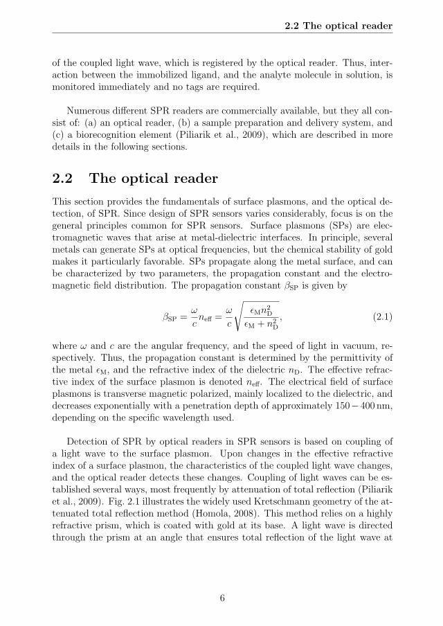
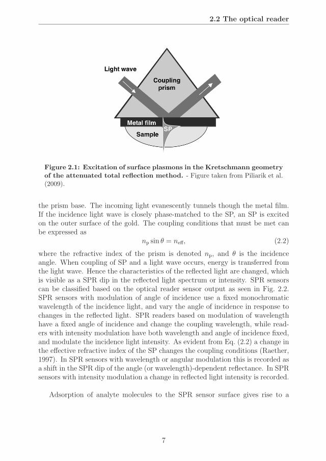
Detection of SPR by optical readers in SPR sensors is based on coupling ofa light wave to the surface plasmon. Upon changes in the effective refractiveindex of a surface plasmon, the characteristics of the coupled light wave changes,and the optical reader detects these changes. Coupling of light waves can be es-tablished several ways, most frequently by attenuation of total reflection (Piliariket al., 2009). Fig. 2.1 illustrates the widely used Kretschmann geometry of the at-tenuated total reflection method (Homola, 2008). This method relies on a highlyrefractive prism, which is coated with gold at its base. A light wave is directedthrough the prism at an angle that ensures total reflection of the light wave at
6
18
2.2 The optical reader
Figure 2.1: Excitation of surface plasmons in the Kretschmann geometryof the attenuated total reflection method. - Figure taken from Piliarik et al.(2009).
the prism base. The incoming light evanescently tunnels though the metal film.If the incidence light wave is closely phase-matched to the SP, an SP is excitedon the outer surface of the gold. The coupling conditions that must be met canbe expressed as
np sin θ = neff, (2.2)
where the refractive index of the prism is denoted np, and θ is the incidenceangle. When coupling of SP and a light wave occurs, energy is transferred fromthe light wave. Hence the characteristics of the reflected light are changed, whichis visible as a SPR dip in the reflected light spectrum or intensity. SPR sensorscan be classified based on the optical reader sensor output as seen in Fig. 2.2.SPR sensors with modulation of angle of incidence use a fixed monochromaticwavelength of the incidence light, and vary the angle of incidence in response tochanges in the reflected light. SPR readers based on modulation of wavelengthhave a fixed angle of incidence and change the coupling wavelength, while read-ers with intensity modulation have both wavelength and angle of incidence fixed,and modulate the incidence light intensity. As evident from Eq. (2.2) a change inthe effective refractive index of the SP changes the coupling conditions (Raether,1997). In SPR sensors with wavelength or angular modulation this is recorded asa shift in the SPR dip of the angle (or wavelength)-dependent reflectance. In SPRsensors with intensity modulation a change in reflected light intensity is recorded.
Adsorption of analyte molecules to the SPR sensor surface gives rise to a
7
19

2.3 The sample preparation and delivery system
Figure 2.2: SPR sensors based on modulation of (a) wavelength, (b)angle of incidence, and (c) light intensity. - Figure taken from Piliarik et al.(2009).
change in the effective refractive index of the surface plasmon, hence the couplingconditions changes, and adsorption of analyte is detected as a change in thereflected light spectrum (wavelengths and angular modulating SPR sensors) orin the reflected light intensity (intensity modulating SPR sensors). A change inrefractive index is commonly measured in resonance units (RU). The recordedsignal has been demonstrated to be proportional to the surface concentration ofmacromolecules with 1 RU corresponding to approximately 1 pgmm−2 (Stenberget al., 1991). In this way, SPR sensors directly measure the mass concentrationof adsorbed analyte, without the need for labeling of interaction partners.
2.3 The sample preparation and delivery sys-
tem
The preparation and delivery system of SPR sensors ensure that the solubilizedanalyte molecules are delivered to the SPR sensor chip. In general, SPR sensorsfunction either via a cuvette system or a flow cell system (Ward and Winzor,2000). In cuvette-based SPR sensors, a fixed volume of sample is injected into acuvette, where the analyte interacts with the ligand on the sensor surface underno-flow conditions. Stirring while measuring is typical to reduce the effect ofmass transport on the data. In flow cell based sensors, the sensor surface is
8
20

2.4 The biorecognition element
placed in a flow cell unit, which is continuously perfused with sample at flowrates ranging from 1 − 100μLmin−1. The analyte diffuses to the sensor surfacewhere it interacts with the ligand molecules. The latter setup is the focus pointof the present thesis.
2.4 The biorecognition element
The biorecognition element of SPR readers constitutes ligand molecules, whichhave been immobilized on the solid surface of the SPR reader. The biorecognitionelement is brought in contact with analyte molecules in solution via the deliverysystem to allow complex formations. The choice of ligand molecule (or biorecog-nition element), and the method of immobilization, have important consequencesfor the sensitivity and detection limit of the SPR sensor (Piliarik et al., 2009).They should be carefully chosen for the purpose of ones study, taking factors suchas affinity and specificity for the analyte, and stability of biological function, intoconsideration. Antibodies are the most frequently used biorecognition element(Robelek, 2009), but numerous biosensor chips are commercially available withvarious immobilized ligands, including protein, low molecular weight molecules,membrane-associated molecules, carbohydrates, virus particles, and nucleic acids.
2.5 Analysis of interactions at lipid surfaces by
use of SPR spectroscopy
Molecular interactions can be detected and analyzed by an array of techniques.SPR sensors hold the advantage that labeling of the interaction partners is notnecessary. This is particularly important when studying proteins, where the at-tachment of labels can interfere with protein function (Kodoyianni, 2011). More-over, the technique allows one to analyze the kinetics of molecular interactions,i.e. the association and dissociation (or similarly adsorption and desorption)constants. Two major fields where SPR sensors are widely used are the detec-tion and identification of biological analytes, and the biophysical characteriza-tion of biomolecular interactions. The SPR technique has primarily been usedto study interactions between proteins (Besenicar et al., 2006), but advancesin preparation and commercialization of sensor chips now also allow studies ofprotein-membrane, protein-nucleic acid, protein-carbohydrate, and protein-smallmolecule interactions (Besenicar et al., 2006). This section focuses on presentingthe use of SPR sensors in studies of protein-lipid interactions, which is the focusarea of the experimental part of the thesis, presented in chapter 5. The quanti-tative analysis of SPR data is presented in detail later in the thesis.
9
21

2.5 Analysis of interactions at lipid surfaces by use of SPRspectroscopy
Many biological processes, as well as technological applications, such as fooddigestion and detergent activity of proteins take place at a lipid interfaces. Fur-thermore, important biological interactions often involve receptors embedded inmembranes, and numerous important drug targets are in fact membrane proteins(Cooper, 2004). Accordingly, there has been an increasing interest for apply-ing SPR in studies of protein interactions with lipid surfaces. Lipid surfaces onSPR sensor chips are generally made from one of three principles: 1) hybridbilayer membranes (HBM), which can be made by applying lipid vesicles to a hy-drophobic coating of the sensor chip gold surface (Plant, 1993; Plant et al., 1995;Terrettaz et al., 1993; Cooper et al., 1998). 2) Immobilization of lipid bilayers(Lang et al., 1994; Bunjes et al., 1997). 3) Immobilization of liposomes (Cooperet al., 2000; Graneli et al., 2004). The first commercially available sensor chip,designed for studying interactions with lipids, was the HPA chip launched by Bi-acore. The HPA chip design is based on depositing a monolayer of self-assembledalkanethiols onto the gold surface of a sensor chip. The self-assembled monolayer(SAM) enable HBM formation when the user applies lipid vesicles. The lipid vesi-cles spontaneously adsorb to the SAM by hydrophobic interactions between theSAM and the hydrophobic acyl chain. The polar head groups of the vesicle lipidsthereby comprise the membrane/solution interface. The HBM surface has somedesirable qualities, as it is very stable and homogenous with few defects in thelipid monolayer, and resists nonspecific binding of proteins like BSA (Plant et al.,1995; Terrettaz et al., 1993; Cooper et al., 1998). Cooper et al. (1998) thoroughlyinvestigated the formation of lipid monolayers on the HPA chip, using differentlipid vesicles preparation methods. They also demonstrated that the correlationbetween deposited lipid, and the observed response (number of response units,RU), was similar to that of proteins. A monolayer of lipids corresponds to a de-posited mass of 2.0 ngmm−2, giving rise to a response of about 2200 RU. The HPAsensor chip constitute a very simple and robust membrane model (Cooper, 2004),but has some limitations in its membrane mimetic properties, as it only consistsof a supported monolayer. Membrane mimetic properties are particularly desiredin biological research, where understandings of protein interactions with (or in)cellular membranes or micelles are sought. A significant advantage of sensor chipswith immobilized membrane bilayer or liposomes is that they allow reconstitu-tion of functional transmembrane proteins within the lipid surface (Heyse et al.,1998; Lang et al., 1994; Stora et al., 1999). This is particularly important forstudying interactions with membrane proteins, as they often require the lipidenvironment to retain their functional and structural integrity Cooper (2004).Various techniques for immobilization of membrane bilayers and liposomes havebeen developed and are reviewed by Besenicar et al. (2006); Cooper (2002). Atpresent, the most frequently used sensor chip in protein-membrane studies is the
10
22
2.6 SPR in the present thesis
L1 chip from Biacore, which is designed to immobilize liposomes or membranepreparations from cell lysates (Besenicar and Anderluh, 2010). Studies of directinteraction between a protein and a lipid surface often seek information about ei-ther lipid specificity or about membrane binding motifs of the protein (Besenicaret al., 2006). Lipid specificity can be addressed by modulation of the lipid compo-sition of the biorecognition element, and has been studied for instance for toxins(Bakrac et al., 2008; Kuziemko et al., 1996) and amyloid protein (Aguilar andSmall, 2005). Identification of amino acids involved in the binding process ofa protein to lipid surfaces has been identified for a number of proteins, usingmutagenesis to generate genetically modified protein variants, which are thencharacterized using SPR sensors (Bakrac et al., 2008; Jones et al., 2005; Stahe-lin and Cho, 2001). Thus, Stahelin and Cho (2001) investigated the importanceon ionic, aromatic, and aliphatic amino acids for the binding of phospholipaseA2 to immobilized liposomes. They proposed a general model for protein at-tachment to membranes, where electrical interactions between aromatic aminoacids and a zwitterionic membrane initially bring the protein to the membranesurface. Subsequent hydrophobic interactions between aromatic and aliphaticresidues, and the hydrophobic lipids of the membrane, are responsible for a firmprotein attachment. Other applications of SPR sensors within the field of protein-membrane interactions include analysis of initial binding of pore-forming proteinsto membranes (Anderluh et al., 2003), binding of coagulation factor VIII to thephospholipid surfaces (Saenko et al., 2001), membrane binding of amyloid pro-tein and amylogenic peptides (Aguilar and Small, 2005; Mozsolits and Aguilar,2002; Mozsolits et al., 2003). Finally, numerous interactions with reconstitutedtransmembrane proteins have been studies with SPR sensors (Heyse et al., 1998;Stora et al., 1999; Cooper, 2004; Salamon et al., 1999; Besenicar et al., 2006; Choet al., 2001).
2.6 SPR in the present thesis
In the experimental part of the present Ph.D. project surface plasmon resonanceSPR spectroscopy (Biacore) is applied to study adsorption dynamics of lipase,and competitive adsorption dynamics of lipase and surfactants, on model hy-drophobic surfaces established on the Biacore HPA chip (see chapter 5 for a moredetailed description). While the Biacore SPR apparatus is capable of capturingqualitative adsorption behavior, quantitative studies of chemical rate constantsand equilibrium constants are more challenging. Inconsistencies in derived rateconstants have lead to both experimental and theoretical investigations of theeffect of convection and diffusion of the binders in the microfluidic flow cell, i.e.mass transport, on the SPR signal (Schuck and Minton, 1996; Myszka et al.,
11
23

2.6 SPR in the present thesis
1998 Aug). Significant progress was made by the application of a theoreticalquasi-steady-state approximation. This approximation has been richly adoptedfor Biacore data analysis due to its simplicity (Schuck, 1996; Schuck and Minton,1996; Mason et al., 1999; Noinville et al., 2010; Myszka et al., 1998 Aug; Gold-stein et al., 1999 Sep-Oct). However, practice in the biochemical society still, to alarge degree, consists of empirical and qualitative studies (Rich and Myszka, 2010,2008, 2007). The next chapter provides an in-depth description of the theoreticalmodeling used for SPR data analysis.
12
24

Chapter 3
Mathematical modeling oftransport phenomena insurface-based biosensors
This chapter presents a theoretical and computational investigation of convection,diffusion, and adsorption in surface-based biosensors. We study the transportdynamics in a model geometry designed to mimic the actual geometry used inthe Biacore SPR apparatus. As a novel feature the finite distance from the inlet ofthe microfluidic flow cell to the sensor surface is included. The evolution equationsare introduced, and subsequently made nondimensional, leading to a number ofnondimensional parameters, which will be subject to an in-depth parameter studyduring the chapter. An approximate quasi-steady theory, which is widely adoptedin the surface-based biosensor community, is reviewed. Additionally, an analyticalsolution, which to our knowledge has not been published before, is presented.A nondimensional formulation of the quasi-steady theory reveals the importantnondimensional parameter, known as the Damkohler number, which is sometimesreferred to as the limit coefficient. An expression of the Damkohler number isderived in terms of the Biot number, the Peclet number, and the model geometry.The ability of the quasi-steady theory to capture convective and diffusive masstransport in the surface-based biosensor is thoroughly tested, by comparison withnumerical simulations of the transient dynamics. In this way the consequencesof using the quasi-steady theory for experimental data fitting in both kineticallylimited and convection-diffusion limited regimes are properly quantified. Theresults clarify the conditions under which the quasi-steady theory lack credibility.In extension to the well known fact that credibility is altered under convection-diffusion limited conditions, we also show how the ratio of the inlet concentrationto the maximum surface capacity is critical for reliable use of the quasi-steadytheory.
13
25
3.1 System geometry and two-dimensional approximation
x
y
h
wl
v
2D model
SPR chip
v(y)
x
y zlc
wc
lc
(a)
(b)
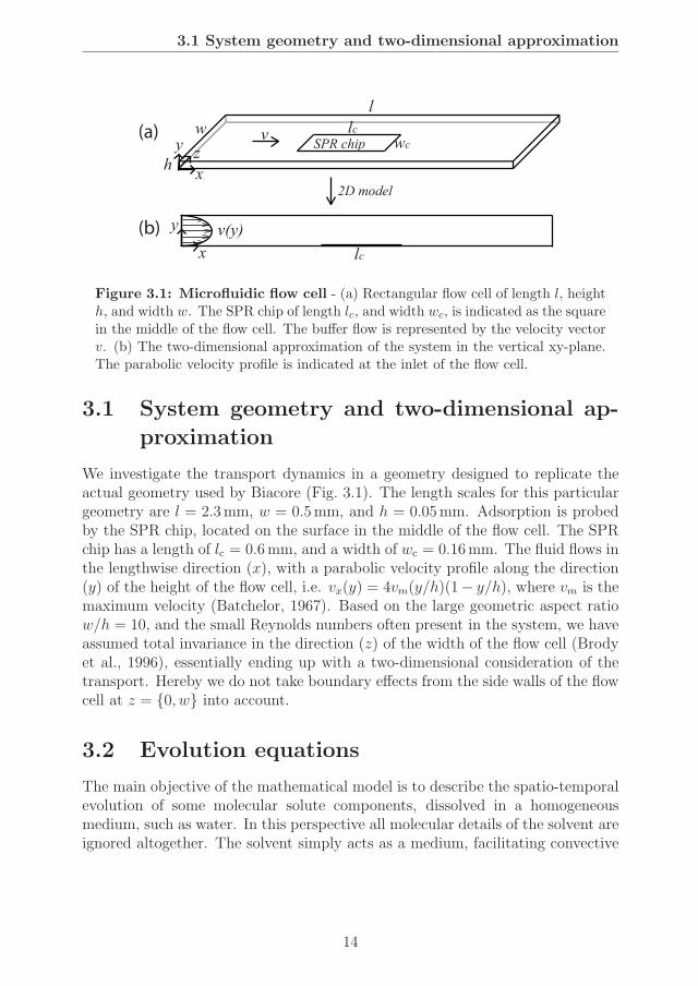
Figure 3.1: Microfluidic flow cell - (a) Rectangular flow cell of length l, heighth, and width w. The SPR chip of length lc, and width wc, is indicated as the squarein the middle of the flow cell. The buffer flow is represented by the velocity vectorv. (b) The two-dimensional approximation of the system in the vertical xy-plane.The parabolic velocity profile is indicated at the inlet of the flow cell.
3.1 System geometry and two-dimensional ap-
proximation
We investigate the transport dynamics in a geometry designed to replicate theactual geometry used by Biacore (Fig. 3.1). The length scales for this particulargeometry are l = 2.3mm, w = 0.5mm, and h = 0.05mm. Adsorption is probedby the SPR chip, located on the surface in the middle of the flow cell. The SPRchip has a length of lc = 0.6mm, and a width of wc = 0.16mm. The fluid flows inthe lengthwise direction (x), with a parabolic velocity profile along the direction(y) of the height of the flow cell, i.e. vx(y) = 4vm(y/h)(1− y/h), where vm is themaximum velocity (Batchelor, 1967). Based on the large geometric aspect ratiow/h = 10, and the small Reynolds numbers often present in the system, we haveassumed total invariance in the direction (z) of the width of the flow cell (Brodyet al., 1996), essentially ending up with a two-dimensional consideration of thetransport. Hereby we do not take boundary effects from the side walls of the flowcell at z = {0, w} into account.
3.2 Evolution equations
The main objective of the mathematical model is to describe the spatio-temporalevolution of some molecular solute components, dissolved in a homogeneousmedium, such as water. In this perspective all molecular details of the solvent areignored altogether. The solvent simply acts as a medium, facilitating convective
14
26

3.2 Evolution equations
and diffusive transport of the solute components. A continuum considerationof some solute component i leads to the definition of two dependent field vari-ables, namely the bulk concentration field ci = ci(x, y, t), and the correspondingsurface concentration field γi = γi(x, t), where t is time. We name the bulk do-main Ω, and the surface domains {∂Ω, ∂Ωads}, referring to respectively insulatingnon-adsorbing surfaces, and surfaces where adsorption takes place. The spatio-temporal evolution of the bulk concentration field ci(x, y, t) is governed by theconvection-diffusion equation
∂ci∂t
+ vx(y)∂ci∂x
= Di∇2ci, Ω (3.1)
where the Laplacian ∇2 = ∂2/∂x2+∂2/∂y2, and Di is the diffusion coefficient formolecular component i. The boundary conditions for the bulk concentration aregiven by
∂ci∂y
= 0, ∂Ω (3.2a)
−Di∂ci∂y
= −Ai(γi, ci, . . .), ∂Ωads (3.2b)
The former is simply a no-flux condition, whereas the latter is a balance betweendiffusive flux perpendicular to the surface and net adsorption rate, captured in theadsorption term Ai(γi, ci, . . .) in Eq. (3.5). At the inlet of the flow cell, at x = 0,the concentration is equal to the injection concentration, ci = ci,0. At the outletof the flow cell, x = l, we assume free convection, i.e. essentially ∂ci/∂x = 0.The spatio-temporal evolution of the surface concentration field γi = γi(x, t) isgoverned by the adsorption-diffusion equation
∂γi∂t
− ∂
∂x
[Di,s
∂γi∂x
]= Ai(γi, ci, . . .), ∂Ωads (3.3)
where Di,s is the surface diffusion coefficient of molecular component i, which ingeneral can be a function of both the independent variables, x and t, as well asthe dependent variables γi, ci, . . .. The adsorption term A(γi, ci, . . .) representsthe net rate of change of surface concentration due to adsorption and desorption.A particular functionality of A(γi, ci, . . .) is determined by the kinetics of somechosen adsorption-desorption scheme, and can in general include arbitrarily com-plex surface kinetics. Particular functionalities of A(γi, ci, . . .) are provided forunimolecular and bimolecular systems respectively in section 3.3.1 and section3.4.1. Finally, no-flux boundary conditions for γi, i.e. ∂γi/∂x = 0 are imposedat the end of the adsorbing domain, i.e. surface bound molecules only leave thechip by desorption.
15
27
3.3 Unimolecular systems
Importantly, the total surface concentration Γ, which is the natural measureof a surface-based biosensor, is given by the sum
Γ =∑i
γi. (3.4)
3.3 Unimolecular systems
In this section the general evolution equations introduced in chapter 3.2 are ana-lyzed in considerable detail for a single molecular solute component. This case isreferred to as a unimolecular system. First, the adsorption kinetics is presented.Then, nondimensional formulations of the unimolecular evolution equations arepresented. This is followed by an order of magnitude estimation of the nondimen-sional parameters. The section ends with a presentation of the weak formulationof the unimolecular evolution equations, which is used for implementation of thefinite element method in the ComSol/MatLab computational software.
3.3.1 Surface adsorption kinetics
The adsorption kinetics has to be modeled by a phenomenological model, whichultimately captures experimental data and thereby provides reasonable and con-sistent phenomenological parameters. The standard adsorption model that con-tains the feature of a maximum surface capacity γm is the Langmuir adsorptionmodel. This model is essentially a first order scheme between bulk molecules atthe interface c|y=0 and free surface space (γm − γ), with adsorption rate constantka and desorption rate constant kd. For a single molecular component this firstorder model may be written in the form
A(γ, c) = kac|y=0(γm − γ)− kdγ. (3.5)
When c|y=0 is independent of γ this is a linear relation between A(γ, c) and γ.This particular adsorption model is a local theory in both space and time, i.e. theevolution of γ at (x, t) depends only on the present state at (x, t). The ultimategoal is often to obtain consistent values for the triplet (ka, kd, γm) of phenomeno-logical parameters from experimental biosensor data. In this linear model theadsorption and desorption rate constants, ka and kd respectively, are assumedunaltered by the density on the surface. In reality on might expect interactionsbetween adsorbed particles at high densities. In spite of its simplicity, however,it has been argued that this model is general enough to explain the majority ofadsorption/desorption processes in molecular biology (Gervais and Jensen, 2006).Substituting Eq. (3.5) into Eq. (3.3) and Eq. (3.2b), these two equations togetherwith Eq. (3.1), and the remaining boundary conditions, form a nonlinear system
16
28

3.3 Unimolecular systems
of partial differential equations for the concentration fields ci(x, y, t) and γi(x, t).The system is in general of such complexity that a numerical study is necessaryfor detailed analysis.
3.3.2 Nondimensional parameterization
Nondimensional formulations are developed for a more comprehensible parame-terization of the unimolecular evolution equations. Two different nondimensionalformulations are introduced and discussed.
Nondimensional parameterization: kinetic scaling
In order to put the evolution equations on nondimensional form, we introducethe following spatial and temporal scales:
x =x
h, y =
y
h, t = kac0t. (3.6)
Note in particular, that time has been made nondimensional by the adsorptionrate. For the dependent concentration variables we introduce the following scaleddependent variables:
c =c
c0, γ =
γ
γm. (3.7)
In terms of these nondimensional variables, and the definitions f(y) = 4y(1− y),
∇2= ∂2/∂x2 + ∂2/∂y2 we obtain the nondimensional evolution equation for the
bulk concentration field
Bic0∂c
∂t+ Pef(y)
(∂c
∂x
)= ∇2
c, Ω (3.8)
with the boundary condition in Eq. (3.2b) given by
∂c
∂y
∣∣∣∣y=0
= Bic|y=0(1− γ)−KBiγ, ∂Ωads (3.9)
The nondimensional evolution equation for the surface concentration field is givenby
∂γ
∂t− ∂
∂x
[dsBic0
∂γ
∂x
]= c|y=0(1− γ)−Kγ, ∂Ωads (3.10)
The remaining boundary conditions are easily translated into the nondimensionalform. These nondimensional evolution equations are parameterized by the fol-
17
29

3.3 Unimolecular systems
lowing five nondimensional groups.
Pe = vmh/D, (3.11a)
Bi = kaγmh/D, (3.11b)
c0 = c0h/γm, (3.11c)
K = kd/kac0, (3.11d)
ds = Ds/D. (3.11e)
The Peclet number Pe measures the ratio of transport by convection to perpendic-ular diffusion, and is essentially the nondimensional flow rate. The Biot numberBi measures the ratio of adsorption rate to diffusion along the height of the flowcell, and is essentially the nondimensional adsorption rate constant. c0 is a nondi-mensional inlet concentration. In the limit of no flow, c0 is the reciprocal of thefraction of the height h needed to fill the surface up to γ = γm. This interpreta-tion explains the close relationship between c0 and the so called depletion depthintroduced by Alvarez et al. (2010). K is the kinetic equilibrium constant. ds isthe ratio of the surface and bulk diffusion coefficients, and if Ds < D, ds ∈ {0, 1}measures the hindrance of diffusion caused by the presence of the surface. In-terestingly, the magnitude of the transient term in Eq. (3.8) is weighed by theproduct c0Bi = kac0h
2/D, essentially meaning that adsorption dynamics for largeinlet concentrations of molecules with a high affinity to the surface evolves in atransient regime. This result is supported by Squires et al. (2008).
Dimensionless parameterization: diffusion scaling
Following a similar approach as above, but with the difference of scaling timewith a diffusion time, i.e. t = Dt/h2, the dimensionless evolution equation forthe bulk concentration field takes the form
∂c
∂t+ Pef(y)
(∂c
∂x
)= ∇2
c, Ω (3.12)
while the boundary condition in Eq. (3.2b) is now given by
∂c
∂y
∣∣∣∣y=0
= Bic|y=0(1− γ)−KBiγ, ∂Ωads (3.13)
The dimensionless evolution equation for the surface concentration field becomes
∂γ
∂t− ∂
∂x
[ds∂γ
∂x
]= Bic0c|y=0(1− γ)−KBic0γ, ∂Ωads (3.14)
The correspondence between the time scales for kinetic scaling (ks) and diffusionscaling (ds) is
tks= t
dskac0h
2/D = Bic0tds. (3.15)
18
30
3.3 Unimolecular systems
Kinetic scaling or diffusion scaling?
The kinetic scaling of time leads to a dimensionless formulation which is par-ticularly advantageous in the regime of kinetically limited dynamics. Generallyspeaking, kinetically limited dynamics is obtained for small Bi numbers (Bi � 1)and/or large Peclet numbers (Pe � 1). Kinetically limited dynamics is, opposedto convection-diffusion limited dynamics, characterized by an independence ofthe flow rate, i.e. the Peclet number, and a scaling of the dynamics with theBiot number. This dynamical behavior is referred to as a kinetic scaling, which istherefore also the terminology used for this particular dimensionless formulation.If, on the other hand, the adsorbing molecules have a very high affinity to thesurface, such as in the case of hydrophobic proteins in aqueous solution, Bi � 1.In this limit the dynamics is convection-diffusion limited, which is characterizedby an independence of adsorption rate, i.e. Biot number, and a scaling of thedynamics with the Peclet number. In this limit it is advantageous to use thediffusion scaling of time.
Disregarding the dynamical limit of the system, there are other pros and consfor applying the two different time scales. As seen below, an approximation ofquasi-steady-state in the bulk transport dynamics leads to a theory, which adoptsa minimal number of dimensionless parameters using kinetic scaling. Hence ki-netic scaling is advantageous when working with the quasi-steady theory. This isconsistent with the fact that the quasi-steady-state approximation is only theo-retically supported for kinetically limited dynamics. This is further elaborated onin section 3.5. However, concerning practical use of the theory for experimentaldata fitting, we remark that ka is usually a parameter one wishes to determinefrom an adsorption experiment, and is thereby unknown a priori. Hence, kineticscaling is not practical for experimental data fitting - an issue avoided by us-ing diffusion scaling. Dependent on the experimental regime it might as well bepreferable to present and fit experimental data unscaled.
3.3.3 Estimates of nondimensional parameters
In this section we estimate some reasonable values for the dimensionless num-bers. Concerning typical operating conditions, flow rates are in the range Q =1 − 100μLmin−1, which amounts to maximum velocities of vm = 3Q/2hw =10−3 − 10−1 ms−1. Injection concentrations typically range from c0 = 10−1 −102 μM. To proceed we need to consider a model binder. We take as an ex-ample a globular protein with a diameter of 2R = 5nm, and molecular weightMw = 30 kDa = 3 × 10⁴ gmol−1. A simple estimate of the maximum surfacecapacity γm is simply the weight of one molecule divided by its diameter squared.
19
31

3.3 Unimolecular systems
Viz, γm = Mw/4NAR2 ≈ 2 × 10³ μgm−2, where NA is the Avogadro number.
However, in biochemical studies the surface of the chip, or the dextran layer, issometimes prepared with a relatively low number of binding sites, with the aimof reducing rebinding probability and neighbor interactions among the adsorb-ing binders. This implies that the above estimate for γm, which is based on apacking occurring for e.g. self-assembled monolayers, represents an upper limit.In several applications the maximum surface capacity can be significantly lower.The diffusion coefficient can be estimated from the Stokes-Einstein relation. Inaqueous solution at room temperature the dynamic viscosity is μ ≈ 10−3 Nsm−2,and T ≈ 300K, hence D = kBT/6πμR ≈ 10−10 m2s−1.
Based on the above values we can estimate the regime of the dimensionless num-bers. By choosing c0 ≈ 1μM, we obtain c0 = coh/γm ≈ 1, in the case of closepacking on the surface. For surfaces prepared with a lower number of bindingsites c0 > 1. For the Peclet number we obtain Pe = vmh/D ≈ 5× 10² − 5× 10⁴.
3.3.4 The weak formulation
The weak formulation of the unimolecular evolution equations is derived usingthe diffusion scaling. The kinetic scaling can later be obtained by a straightfor-
ward rescaling of time tks= Bic0t
ds. The overline notation for the dimensionless
variables is skipped for clarity. The first step of obtaining the weak form is bymultiplication with a test function and integrating over the domain on which thefunction is defined. For the bulk field we get∫
Ω
c∂c
∂tdA+
∫Ω
Pef(y)c
(∂c
∂x
)dA =
∫Ω
c∇×∇c dA
The second step is to reduce the order of the differential equation by integrationby parts of the highest order derivative and using Gauss’ theorem. In this way thesecond order derivative is removed, such that the function c can be approximatedby linear shape functions, whose first order derivatives have jump discontinuities.The partial integration yields∫
Ω
c∇×∇c dA =
∫∂Ω
c∇c× n ds−∫Ω
∇c×∇c dA
Finally, the terms involving temporal respectively spatial derivatives are collectedon the left respectively right hand side of the equation, viz∫
Ω
c∂c
∂tdA =
∫∂Ω
c∇c× n ds−∫Ω
[∇c×∇c+ Pef(y)c
(∂c
∂x
)]dA (3.16)
20
32
3.4 Bimolecular systems
The boundary integral, i.e. the first term on the right hand side, essentiallycontains the boundary conditions for the bulk field. So far nothing has been saidabout the test functions c. The test functions c is chosen to vanish at boundarieswhere the function c satifies Dirichlet conditions, but not elsewhere. Hence
c = 0, at x = 0.
Also, for the insulating surfaces, as well as for the outlet with convective flux,the homogeneous Neumann boundary conditions ∇c × n = 0 translate into avanishing contribution to the boundary integral. Clearly, the integrand in theboundary integral is non-zero only at adsorbing surfaces where
∂c
∂y
∣∣∣∣y=0
= Bic|y=0(1− γ)−KBiγ ∂Ωads (3.17)
For the sake of completeness the weak formulation of the bulk field is summarizedin∫
Ω
c∂c
∂tdA =
∫∂Ωads
[Bic|y=0(1−γ)−KBiγ
]dx−
∫Ω
[∇c×∇c+Pef(y)c
(∂c
∂x
)]dA
(3.18)The weak formulation for the surface field is obtained in a similar way, howeversince the equation is naturally first order, it is simply∫
∂Ωads
γ∂γ
∂tdx =
∫∂Ωads
γ
[∂
∂xds∂γ
∂x+ Bic0c|y=0(1− γ)−KBic0γ
]dx (3.19)
Eqs. (3.18) and (3.19) constitute the weak formulation of the unimolecular evo-lution equations. The mathematical goal is to find a set of functions (c, γ) thatsatisfies Eqs. (3.18) and (3.19), as well as c = 1 at x = 0, for all sufficientlysmooth functions (c, γ), where c has the property that it vanishes at x = 0. Thistask is performed by an implementation of the weak formulation of the evolutionequations in the ComSol/MatLab computational software. More details onthe finite element method is outside the scope of the present thesis. Numericalanalysis based on an implementation of the weak form is presented in chapter 4.
3.4 Bimolecular systems
In this section the general evolution equations, introduced in chapter 3.2, aredeveloped for a bimolecular system, i.e. two molecular solute components. Thesolute components in the bulk phase are assumed to be dissolved to a dilutestate, such that intermolecular interactions of the solutes can be ignored. On the
21
33

3.4 Bimolecular systems
surface the solute particles are close together, i.e. molecular length scales, for anextended period of time, hence interactions on the surface have to be taken intoaccount. In this way, the introduction of an additional component only alters theadsorption kinetics. Following a presentation and discussion of the adsorptionkinetics, nondimensional formulations of the bimolecular evolution equations arepresented along with an order of magnitude estimation of the nondimensionalparameters.
3.4.1 Surface adsorption kinetics
The main scope of the bimolecular system is to model competitive adsorption oftwo species. The model is motivated by experiments on the competitive adsorp-tion of lipase enzymes and surfactants, which is explained in detail in chapter 5,and in particular section 5.4. Like for the unimolecular system the adsorptionkinetics is modeled by a phenomenological model, designed as an attempt to con-sistently capture experimental data and provide reasonable and consistent phe-nomenological parameters. For the sake of clarity the kinetic rate equations forthe two-component competitive adsorption/desorption dynamics are developed,with no convective-diffusive transport in mind, and then subsequently integratedinto the full theoretical spatio-temporal framework.
When two different species are present on the surface together, it has to betaken into account that they will give different response in the SPR measurementper unit area. This is actually the only way to distinguish between differentadsorbed species on the surface, as SPR spectroscopy is a label-free method asdescribed in chapter 2. A simple approach to cope with this challenge is simply todevelop the kinetic rate equations in terms of the relative surface areas exerted bythe different species. Defining the surface area fractions for enzyme and surfactantas respectively θe and θs, the kinetic rate equations can be written generally as
dθedt
= fe(θe, θs, ce, cs; ke,i) (3.20a)
dθsdt
= fs(θe, θs, ce, cs; ks,i) (3.20b)
where the functions fe and fs are the rate of change of the area-based surface con-centrations due to adsorption and desorption kinetics. These terms, in general,depend on the concentration field variables and are constrained by some para-meters ke,i, ks,i that include adsorption and desorption rate constants, maximumsurface capacities, and other possible constraints.
22
34

3.4 Bimolecular systems
Integrating the kinetics with bulk transport
The source term Ai in Eq. (3.3) is simply the rate of change of mass-based sur-face concentration due to adsorption and desorption kinetics, hence in order tointegrate the two-component kinetic rate equations into the full spatio-temporalframework we simply put
Ai = γm,idθi/dt, (3.21)
where γm,i is maximum surface capacity of the particular specie i. Under purelykinetically limited conditions, with no account of convective-diffusive transport,the surface concentrations are only functions of time, and Eqs. (3.20) are simplytwo coupled ordinary differential equations (ODE’s) for the temporal evolutionof the surface concentrations. The general framework is written as
Ae = γm,efe(θe, θs, ce, cs; ke,i) (3.22a)
As = γm,sfs(θe, θs, ce, cs; ks,i) (3.22b)
Kernel of the two-component model
Motivated by experimental results the surfactant system is modeled by the simpleLangmuir adsorption/desorption model presented in section 3.3.1. Also, the lipaseenzymes are known to adsorb irreversibly in the absence of surfactants. Takinginto account that free surface space is given by (1 − θs − θe) the dynamics ismodeled by the following system of adsorption rate equations
dθedt
= ka,ece(1− θs − θe) (3.23a)
dθsdt
= ka,scs(1− θs − θe)− kd,sθs (3.23b)
In terms of the mass-based concentration fields we obtain
Ae = ka,ece(γm,e − γe − γm,e
γm,s
γs) (3.24a)
As = ka,scs(γm,s − γs − γm,s
γm,e
γe)− kd,sγs (3.24b)
An important aspect, which however deserves attention at this point, is thatthe surfactant forms micelles in solution above the critical micelle concentration(cmc). The micelles, being multimolecular aggregates, diffuse slower, and can beexpected to exhibit a different intrinsic adsorption behavior than that of the singlesurfactant molecules. From this perspective the definition of the bulk surfactantconcentration, and a corresponding adsorption rate constant ka,s, seems dubious.A more thorough theoretical model would take into account the dynamics of
23
35

3.4 Bimolecular systems
micelle formation, and the adsorption/desorption dynamics of single surfactantmolecules and micelles, separately. To keep the complexity level reasonable thisapproach is however avoided in the present work. This decision is actually data-driven. For the experiments done in the present work the pure surfactant systemis reasonably well captured by the Langmuir model as shown in section 5.4. Atwo-component model like Eqs. (3.24), without any displacement of one specieby the other, has been analyzed by Fu and Santore (1998).
First order displacement model
In the presence of surfactants, enzyme desorption is observed. Different mech-anisms, some of which are discussed in chapter 5, have been proposed in orderto explain how surfactants displace enzyme on the surface in a competitive pro-cess. In regards to modeling surface kinetics a mathematical term is needed tocapture this competitive displacement process. The most plain way of modelingthe competitive displacement process is by a first order reaction between surfacebound surfactant and enzyme, in which case a negative term −kcθsθe is added toEq. (3.26a), such that
dθedt
= ka,ece(1− θs − θe)− kcθsθe (3.25a)
dθedt
= ka,scs(1− θs − θe)− kd,sθs (3.25b)
In terms of the mass-based concentration fields we obtain
Ae = ka,ece(γm,e − γe − γm,e
γm,s
γs)− kcγsγm,s
γe (3.26a)
As = ka,scs(γm,s − γs − γm,s
γm,e
γe)− kd,sγs (3.26b)
This model, albeit simple, captures the essence of the competitive adsorption oftwo species, including displacement of one specie by the other.
Coorporative displacement model
The above form of the displacement term, being of first order in both surfactantand enzyme, takes no coorporative behavior of the surfactant into account. Inreality it is well known (see section 5.4) that the surfactant has properties of self-assembly and enhanced surface activity above a certain concentration threshold.It is therefore probable that the displacement is better captured by some higherorder model. One displacement model that has many of the wanted properties
24
36

3.4 Bimolecular systems
0 0.5 1 1.5 20
0.2
0.4
0.6
0.8
1
s
f(s)
s,p = 0.01
s,p = 0.1
s,p = 0.3
Figure 3.2: Coorporative displacement model - Parameters: θs,c = 1, θs,p ={0.01, 0.1, 0.3}
is build from the inverse tangent function. Choosing again a first order form forthe enzyme leads to a competitive term −kcf(θs)θe, where
f(θs) =1
π
[arctan
(θs − θs,cθs,p
)+ arctan
(θs,cθs,p
)](3.27)
This form, in principle, introduces two additional parameters: θs,c, measuringthe surface concentration of surfactant at which the coorporativity enhances itscompetitive properties, as well as θs,p that measures how dramatic the changein competitive properties is. Increasing the value of θs,p leads to a less dramaticchange and vice versa. The functionality of the model is presented in Fig. 3.2. Themodel is chosen such that it goes to zero for vanishing surfactant concentrations,and to unity for large surfactant concentrations. The latter property implies thatkc is a normalized measure of the strength of the displacement.
3.4.2 Nondimensional parameterization
The nondimensional parameterization is done for the first order competitive ad-sorption model, and to keep the number of free parameters to a reasonable mini-mum surface diffusion is neglected. The mathematical formulation of the spatio-temporal problem for the bimolecular system consists of two independent ver-sions of Eq. (3.1) for the two molecular components, respectively. The couplingof the two fields arises from the two versions of the surface evolution equations(Eq. (3.3)), and the boundary flux balance conditions (Eq. (3.2b)). The following
25
37
3.4 Bimolecular systems
spatial and temporal scales are applied:
x =x
h, y =
y
h, t =
Dst
h2(3.28)
Time has been made nondimensional by the surfactant diffusion time across theheight of the flow cell. For the dependent concentration variables we introducethe following scaled variables:
ce =cece,0
, cs =cscs,0
, γe =γeγm,e
, γs =γsγm,s
(3.29)
where ce,0 and cs,0 are the bulk concentrations injected at the inlet of the flowcell (x = 0). The following dimensionless parameters are defined:
Pes =vmh
Ds
: Peclet number based on surfactant diffusion (3.30a)
Bie =ka,eγm,eh
De
: enzyme Biot number (3.30b)
Bis =ka,sγm,sh
Ds
: surfactant Biot number (3.30c)
d =De
Ds
: ratio of enzyme and surfactant diffusion coefficients (3.30d)
kc =kcγm,eh
Dece,0: Nondimensional competition constant (3.30e)
Ks =kd,s
ka,scs,0: surfactant kinetic equilibrium constant (3.30f)
ce,0 =ce,0h
γm,e
: Nondimensional inlet enzyme concentration (3.30g)
cs,0 =cs,0h
γm,s
: Nondimensional inlet surfactant concentration (3.30h)
In terms of these nondimensional variables and parameters, and the definitions
f(y) = 4y(1− y), ∇2= ∂2/∂x2+ ∂2/∂y2 we obtain the nondimensional evolution
equations. For the bulk concentration fields (Eq. (3.1)):
∂ce∂t
+ Pesf(y)∂ce∂x
= d∇2ce, Ω (3.31a)
∂cs∂t
+ Pesf(y)∂cs∂x
= ∇2cs, Ω (3.31b)
26
38

3.5 The quasi-steady theory
The boundary conditions (Eq. (3.2b)) become
∂ce∂y
∣∣∣∣y=0
= Biece|y=0(1− γs − γe)− kcγsγe, ∂Ωads (3.32a)
∂cs∂y
∣∣∣∣y=0
= Biscs|y=0(1− γs − γe)−KsBisγs, ∂Ωads (3.32b)
The nondimensional evolution equations for the surface concentration fields arefinally given by
∂γe
∂t= Biedce,0ce|y=0(1− γs − γe)− kcdce,0γsγe, ∂Ωads (3.33a)
∂γs
∂t= Biscs,0cs|y=0(1− γs − γe)−KsBiscs,0γs, ∂Ωads (3.33b)
Again, the remaining no-flux boundary conditions are trivially translated into thenondimensional form for both molecular components.
3.4.3 Estimates of nondimensional parameters
In this section we estimate some reasonable values for the nondimensional para-meters for the bimolecular system. As for the unimolecular system, flow ratesare in the range Q = 1 − 100μLmin−1, amounting to maximum velocities ofvm = 3Q/2hw = 10−3 − 10−1 ms−1. A diffusion coefficient for the enzyme wasestimated in section 3.3.3, using the Stokes-Einstein relation D = kBT/6πμR ≈10−10 m2s−1. The smaller surfactant molecules diffuse faster. Considering for ex-ample surfactant molecules of linear size 5× 10⁻¹⁰ m, which is one order of mag-nitude smaller than the enzyme, leads to a diffusion coefficient of approximately10−9 m2s−1. This leads to Peclet numbers, based on the surfactant diffusion coef-ficient, of order Pes ≈ 5×10²−5×10⁴, and d = De/Ds ≈ 10−1. Also, from section3.3.3, ce,0 ≈ 1μM, and hence ce,0 = ce,0h/γm,e ≈ 1. The injection concentration ofsurfactant is typically two orders of magnitude higher, dependent on the cmc forthe particular surfactant. In addition, the maximum surface capacity γm,s is typ-ically a few times smaller. A rough estimate may be that cs,0 = cs,0h/γm,s ≈ 100.
The set of parameters (Bie,Bis, kc, Ks) characterizes adsorption, desorptionand competition, and would typically be the quantitative objective of adsorptionexperiments.
3.5 The quasi-steady theory
The theoretical models developed in the earlier sections 3.2, 3.3, and 3.4 all entailnumerical simulations. The models have the mathematical structure of nonlin-
27
39
3.5 The quasi-steady theory
ear systems of partial differential equations, which require somewhat demandingnumerical techniques. Analytical studies of these models are few, hence they areunfit for use in experimental data analysis, and this kind of modeling have there-fore not been widely embraced by the SPR community. This section is concernedwith a widely adopted approximate theory, which we refer to as the quasi-steadytheory.
Ideally one would like to interpret SPR data by assuming simply that theconcentration near the sensor cy=0 is identical to the injection concentration c0.That is, by assuming that there is no resistance to mass transfer. To accountfor the corrections due to some mass transfer resistance, it has been suggested tointerpret data by means of a mass transport model, saying that the overall fluxof solute J to the surface is proportional to the difference between the far fieldconcentration c0, usually taken as the injection concentration, and the concentra-tion close to the surface of the sensor c|y=0, i.e. J = kL(c0 − c|y=0). In fact, thissuggestion is based on a solution to the stationary diffusion-convection equationfor the concentration field c = c(x, y) on a semi-infinite domain x, y ≥ 0
vx∂c
∂x= D
∂2c
∂y2, y > 0. (3.34)
The velocity vx = vx(y) is linearized close to the surface, i.e. vx(y) = γwy,γw being the shear rate at the surface, and the boundary conditions for theconcentration field are c(x, y)|y=0 = const, c(x, y)|x,y→∞ = 0, and c(x, y)|x=0 = c0.The solution consists of a concentration boundary layer close to the surface y = 0,and a flux of solute to the surface J = kL(c0 − c|y=0), where the mass transportparameter kL is given by
kL =2D
Γ(73)
(γw9Dl
)1/3
. (3.35)
This mass transport parameter is often chosen as a free fitting parameter inthe SPR community, although it may in fact be predicted from the operatingconditions. Given a flow rate Q, the shear rate at the wall is
γw =6Q
h2w(3.36)
The coupling of this stationary convection-diffusion solution with the adsorptionkinetics on the surface is performed by loosening up the Dirichlet boundary con-dition c(x, y)|y=0 = const. Letting these bulk particles c|y=0 adsorb, they areconverted into surface particles γ, and a simple mass balance on the surface dic-tates J = dγ/dt = A(γ, c). The critical assumption here is that the adsorption is
28
40
3.5 The quasi-steady theory
so slow, that the bulk concentration on the surface c|y=0 is practically constant,and use of the steady-state flux J = kL(c0 − c|y=0), with kL given by Eq. (3.35),is still reasonable.
Inserting the steady-state flux into the mass balance on the surface yieldskL(c0 − c|y=0) = A(γ, c). In the case of linear kinetics (Eq. (3.5)) this becomesan algebraic equation for c|y=0, with the solution
c|y=0 =kLc0 + kdγ
ka(γm − γ) + kL(3.37)
Substituting this into Eq. (3.5) gives the following nonlinear ordinary differentialequation for the evolution of the surface concentration γ(t)
dγ
dt=
kakLc0(γm − γ)− kdkLγ
ka(γm − γ) + kL(3.38)
Using the kinetic scaling from section 3.3, we can write Eq. (3.38) as
dγ
dt
ks
=1− (1 +K)γ
1 + Da(1− γ)(3.39)
with the additional introduction of the important dimensionless Damkohler num-ber
Da = kaγm/kL, (3.40)
which is the ratio of the adsorption rate and the rate of mass transport to the sur-face, i.e. it measures the limiting effect of convection-diffusion on the adsorptionprocess. If Da � 1 the system is kinetically limited, and if Da � 1 the system isconvection-diffusion limited. Note in particular when Da � 1 Eq. (3.39) becomes
dγ
dt
ks
= 1− (1 +K)γ, Da � 1 (3.41)
which is simply the dimensionless form of Eq. (3.5), i.e. a purely adsorption-limited, linear, first order kinetic process. Also, the initial rate of adsorption,starting from the initial condition of zero surface concentration, γ = 0, is pre-dicted to be
dγ
dt(0)ks =
1
1 + Daor
dγ
dt(0)ks = c0kL
Da
1 + Da(3.42)
Using diffusion scaling the formulation of the quasi-steady theory involves thetwo additional parameters, Bi and c0, viz
dγ
dt
ds
=Bic0(1− γ)−Kγ
Da(1− γ)− 1(3.43)
29
41
3.5 The quasi-steady theory
By combining Eq. (3.39) with Eq. (3.35) we obtain the scaling of the maximumrate of adsorption with Peclet number in the convection-diffusion-limited regime(Da � 1),
max
(dγ
dt
)∼ Pe1/3. (3.44)
3.5.1 Correspondence between the Damkohler, Biot, andPeclet number
The kinetic scaling of the evolution equations (Eqs. (3.8),(3.9),(3.10)) clarifies theassumptions in the quasi-steady theory. By setting Bi = 0 we essentially obtainthe conditions for the solution in Eq. (3.35), i.e. time dependency drops out ofthe bulk convection-diffusion equation, which is consistent with an instantaneousbuild-up of the concentration boundary layer above the adsorbing surface in thequasi-steady theory. In addition, the quasi-steady theory approximates reality bya semi-infinite bulk domain, a linear velocity profile, and equally important, byno inlet distance to the sensor surface. With the exception of the last difference,we expect that the quasi-steady theory can be obtained from a boundary layerperturbation theory. This work has however not been further pursued.
The kinetically scaled quasi-steady theory in Eq. (3.39) is parameterized onlyby the Damkohler number Da, and the equilibrium constant K. As the quasi-steady theory combines steady-state convection-diffusion with adsorption in theDamkohler number, through the mass transport coefficient kL, it is naturallypossible to express the Damkohler number in terms of the Peclet number and theBiot number. First, from Eq. (3.36), γw = 4vm/h. By defining the number α =2(4/9)1/3/Γ(7/3) ≈ 1.2819, the mass transport coefficient kL can be expressed as
kL = α
(vmh
D
)1/3D
l1/3h2/3
Hence the Damkohler number is given by
Da =kaγmkL
= α−1(l/h)1/3 BiPe−1/3 (3.45)
Note that the quasi-steady theory is parameterized by the Damkohler number,and at the same time is based on the assumption Da = 0. It is clear fromEq. (3.45) that the Damkohler number increases linearly with the Biot number,and decreases with the cubic root of the Peclet number. Practically speaking,if the binders are strongly attracted to the surface (large Biot number), it maybe impossible to reduce the Damkohler number significantly by simply increasingthe flow rate, i.e. Peclet number.
30
42
3.5 The quasi-steady theory
3.5.2 Analytical solution of the quasi-steady theory
Eq. (3.39) can be solved analytically in implicit form, i.e. t = t(γ) instead of theexplicit form γ = γ(t). It is determined simply by separation of variables andintegration, with initially γ(t = 0) = 0:
t =Daκγ − (
κ+Da(κ− 1))ln(1− κγ)
κ2(3.46)
where κ ≡ 1+K. For irreversible adsorptionK = 0, κ = 1, the solution condensesinto
t = Daγ − ln(1− γ) (3.47)
This solution may not be so useful for physical insight, but has its practical ad-vantage when performing nonlinear least squares data fitting in the time domain.Data fitting in the time domain involves a numerical solution of the ordinary dif-ferential equation (Eq. (3.39)) at every parameter space iteration, which can beavoided with the implicit solution above. Another option is simply fitting datain the phase plane (Goren et al., 2006 Jan 31). This method does not involvethe solution of Eq. (3.39), is explicit, but as a trade off involves differentiation ofdata.
3.5.3 Note on two-compartment model
The quasi-steady theory captures the qualitative essence of the mass transportproblem in the microfluidic system of surface-based biosensors. In this respect thetheory includes the coupling of convective and diffusive bulk mass transport withadsorption/desorption surface kinetics. To increase the quantitative accuracy ofthe model in the context of fitting data from surface-based biosensor experiments,a two-compartment model has been suggested (Schuck and Minton, 1996; Myszkaet al., 1997 Feb 28, 1998 Aug). In this model the flow cell is divided into twocompartments, an inner compartment directly adjacent to the sensor surface, andan outer compartment spanning the rest of the flow cell. The outer compartmentis modeled with a uniform concentration equal to the injection concentration.Mass transport from the outer to the inner compartment is then modeled by aflux, linear in the concentration difference between the two compartments, likethe quasi-steady flux, with the mass transport coefficient kL. This mass trans-port coefficient is usually chosen as a free fitting parameter. The mass transportbetween the inner compartment and the surface is finally modeled by a first orderkinetic adsorption/desorption scheme like in Eq. (3.5).
The two compartment model shows increased capabilities of fitting experi-mental data (Myszka et al., 1998 Aug). What happens is that the introduc-
31
43
3.5 The quasi-steady theory
tion of the two compartments renders the adsorption process second order, i.e.dγ/dt(t = 0) = 0. The inner compartment needs to receive solute binders fromthe outer compartment before being able to support adsorption onto the sur-face. This second order behavior is consistent with real adsorption experiments,where the concentration boundary adjacent to the SPR surface initially needsto build up by a time-dependent transient transport process. The drawback ofthe two-compartment model is the somewhat arbitrary specification of the innercompartment height, and thereby the definition of the compartments, altogether.Choosing the inner compartment height to zero leads back to the quasi-steadytheory. The shortcomings of the quasi-steady theory, especially in the initialprocess of an adsorption experiment, is analyzed in detail in chapter 4.
32
44
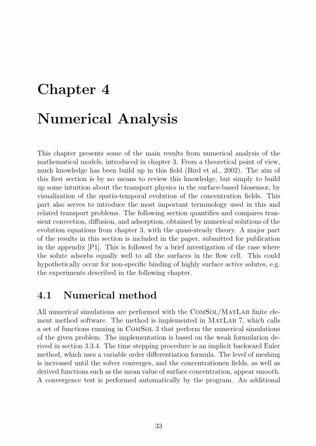
Chapter 4
Numerical Analysis
This chapter presents some of the main results from numerical analysis of themathematical models, introduced in chapter 3. From a theoretical point of view,much knowledge has been build up in this field (Bird et al., 2002). The aim ofthis first section is by no means to review this knowledge, but simply to buildup some intuition about the transport physics in the surface-based biosensor, byvisualization of the spatio-temporal evolution of the concentration fields. Thispart also serves to introduce the most important terminology used in this andrelated transport problems. The following section quantifies and compares tran-sient convection, diffusion, and adsorption, obtained by numerical solutions of theevolution equations from chapter 3, with the quasi-steady theory. A major partof the results in this section is included in the paper, submitted for publicationin the appendix [P1]. This is followed by a brief investigation of the case wherethe solute adsorbs equally well to all the surfaces in the flow cell. This couldhypothetically occur for non-specific binding of highly surface active solutes, e.g.the experiments described in the following chapter.
4.1 Numerical method
All numerical simulations are performed with the ComSol/MatLab finite ele-ment method software. The method is implemented in MatLab 7, which callsa set of functions running in ComSol 3 that perform the numerical simulationsof the given problem. The implementation is based on the weak formulation de-rived in section 3.3.4. The time stepping procedure is an implicit backward Eulermethod, which uses a variable order differentiation formula. The level of meshingis increased until the solver converges, and the concentrationen fields, as well asderived functions such as the mean value of surface concentration, appear smooth.A convergence test is performed automatically by the program. An additional
33
45
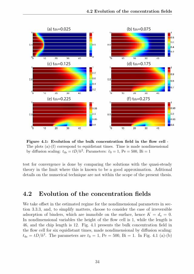
4.2 Evolution of the concentration fields
(a) tds=0.025 (b) tds=0.075
(c) tds=0.125 (d) tds=0.175
(e) tds=0.225 (f ) tds=0.275
Figure 4.1: Evolution of the bulk concentration field in the flow cell -The plots (a)-(f) correspond to equidistant times. Time is made nondimensionalby diffusion scaling: tds = tD/h2. Parameters: c0 = 1, Pe = 500, Bi = 1
test for convergence is done by comparing the solutions with the quasi-steadytheory in the limit where this is known to be a good approximation. Aditionaldetails on the numerical technique are not within the scope of the present thesis.
4.2 Evolution of the concentration fields
We take offset in the estimated regime for the nondimensional parameters in sec-tion 3.3.3, and, to simplify matters, choose to consider the case of irreversibleadsorption of binders, which are immobile on the surface, hence K = ds = 0.In nondimensional variables the height of the flow cell is 1, while the length is46, and the chip length is 12. Fig. 4.1 presents the bulk concentration field inthe flow cell for six equidistant times, made nondimensional by diffusion scaling:tds = tD/h2. The parameters are c0 = 1, Pe = 500, Bi = 1. In Fig. 4.1 (a)-(b)
34
46

4.2 Evolution of the concentration fields
Figure 4.2: Evolution of the surface concentration field at the SPR chip- The curves correspond to the equidistant times from Fig. 4.1 (a)-(f). The abscissaxc is the measure along the x-axis starting at the chip. Parameters: c0 = 1, Pe =500, Bi = 1
we clearly see how the solute is convected by the parabolic velocity flow profile,while diffusion evens out the concentration field at the border to the buffer ini-tially present in the flow cell. As time progresses further, going from Fig. 4.1 (b)to (f), we observe a transient formation of a concentration boundary layer abovethe surface of the adsorbing SPR chip. The adsorption causes a depletion locallyabove the chip. The system approaches a steady-state, where this depletion ofthe solute above the chip is balanced by the convection of fresh solute from theinlet of the flow cell. The physics of this steady-state boundary layer is theoreti-cally well understood (Bird et al., 2002), and forms the basis for the quasi-steadytheory of adsorption, as described in the preceding chapter in section 3.5. Thesteady-state is reached after the surface concentration has saturated, such thatγ = γ/γm = 1. Fig. 4.2 shows the evolution of the surface concentration fieldγ, corresponding to the equidistant times from Fig. 4.1 (a)-(f). For (a) and (b)only a minor amount of solute has adsorbed. From (c) to (f) the surface con-centration increases almost linearly with time, while the surface is still far fromsaturation. The concentration decreases with downstream distance due to theearlier encounter with bulk solute in the beginning of the chip, and the thinnerboundary layer in this region.
Fig. 4.3 compares the bulk concentration field for different parameters at the
35
47
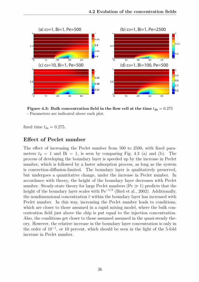
4.2 Evolution of the concentration fields
(a) c0=1, Bi=1, Pe=500 (b) c0=1, Bi=1, Pe=2500
(c) c0=10, Bi=1, Pe=500 (d) c0=1, Bi=100, Pe=500
Figure 4.3: Bulk concentration field in the flow cell at the time tds = 0.275- Parameters are indicated above each plot.
fixed time tds = 0.275.
Effect of Peclet number
The effect of increasing the Peclet number from 500 to 2500, with fixed para-meters c0 = 1 and Bi = 1, is seen by comparing Fig. 4.3 (a) and (b). Theprocess of developing the boundary layer is speeded up by the increase in Pecletnumber, which is followed by a faster adsorption process, as long as the systemis convection-diffusion-limited. The boundary layer is qualitatively preserved,but undergoes a quantitative change, under the increase in Peclet number. Inaccordance with theory, the height of the boundary layer decreases with Pecletnumber. Steady-state theory for large Peclet numbers (Pe � 1) predicts that theheight of the boundary layer scales with Pe−1/3 (Bird et al., 2002). Additionally,the nondimensional concentration c within the boundary layer has increased withPeclet number. In this way, increasing the Peclet number leads to conditions,which are closer to those assumed in a rapid mixing model, where the bulk con-centration field just above the chip is put equal to the injection concentration.Also, the conditions get closer to those assumed assumed in the quasi-steady the-ory. However, the relative increase in the boundary layer concentration is only inthe order of 10−1, or 10 percent, which should be seen in the light of the 5-foldincrease in Peclet number.
36
48

4.3 Transient transport in surface-based biosensors
Effect of inlet concentration
The effect of increasing the nondimensional inlet concentration c0 from 1 to 10,with fixed parameters Bi = 1 and Pe = 500, is seen by comparing Fig. 4.3 (a) and(c). The most notable effect is a decrease in the nondimensional concentrationgradients across the boundary layer.
Effect of Biot number
The effect of increasing the Biot number from 1 to 100, with fixed parametersc0 = 1 and Pe = 500, is seen by comparing Fig. 4.3 (a) and (d). In this case themost notable effect is a more pronounced depletion of the bulk concentration fieldabove the adsorbing chip. This leads to increased nondimensional concentrationgradients across the boundary layer.
4.3 Transient transport in surface-based biosen-
sors
This section is concerned with a numerical investigation of the nonlinear sys-tem of partial differential equations, governing the evolution of the concentra-tion fields. The intention is to simulate the dynamics of real adsorption experi-ments in surface-based biosensors, whereby we use the mean surface concentrationΓ ≡ (1/lc)
∫sensor
γ dx as the central quantifier. Numerical solutions to Eqs. (3.8),(3.9), and (3.10), or similarly Eqs. (3.12), (3.13), and (3.14), are collectivelyreferred to as the simulations. We take offset in the estimated regime for thenondimensional parameters, and to simplify matters choose to consider the caseof irreversible adsorption of binders, which are immobile on the surface, henceK = ds = 0. A particular aim of the investigation is to evaluate the quality ofthe quasi-steady theory by comparison with the simulations. Deviations betweenthe simulations and the quasi-steady theory reveal the effects of the transientdynamics in the simulations, which of course are also present in real adsorptionexperiments. To mimic the case of real adsorption experiments, being fitted bythe quasi-steady theory to reveal an adsorption rate constant ka, we fit the quasi-steady theory to the simulation with Bi as the free fitting parameter, using a leastsquares method. The quasi-steady theory has no chance of fitting initial data,hence the simulation time from the origin of the phase plane to the extremum(highest adsorption rate) is cut off in the fitting procedure, corresponding to typ-ical practice of representing SPR data in the phase plane (Goren et al., 2006Jan 31). The error of the quasi-steady theory is then quantified by the relativedifference between the fitted Bi number and the real Bi number used for the simu-
37
49

4.3 Transient transport in surface-based biosensors
lation. Strictly speaking, we define the error as (Bifit−Bi)/Bi. Being interested inthe kinetics of adsorption the results are most naturally presented and analyzedin the phase plane, spanned by the mean surface concentration Γ, and its timederivative Γ ≡ (1/lc)
∫sensor
∂γ/∂t dx. This representation clearly illustrates thetransient regime, and is the most straightforward approach to analyze deviationsfrom linear adsorption kinetics due to mass transport. The choice of parametersspan both kinetically limited and convection-diffusion limited dynamics. Resultsare presented using both kinetic and diffusion scaling of time, the former leadingto universality for kinetically limited dynamics, and the latter leading to univer-sality for convection-diffusion limited dynamics. Note in particular that purelykinetically limited dynamics, i.e. the linear kinetics in 3.5, is represented by alinear curve in the phase plane. For kinetic scaling this linear curve is the di-agonal from the point (0, 1) on the ordinate to the point (1, 0) on the abscissa.The universality characteristic obtained with kinetic scaling is that this curverepresents the dynamics independent of c0 and Pe for large enough Bi.
4.3.1 Kinetic scaling
Fig. 4.4 contains a representative collection of phase plane curves using kinetic
scaling, i.e. tks= kac0t. Four different simulations for the combinations of concen-
trations c0 ∈ {1, 20}, Bi ∈ {1, 10}, and Pe = 500 are presented (full black line),each in a separate plot, along with the prediction of the quasi-steady theory foridentical parameters (dashed black line), as well as a fit of the quasi-steady theoryto the simulations (dashed gray line). Importantly, the quasi-steady theory scaleslinearly with c0, taken into account in the kinetic scaling of time in 3.39. Hencethe quasi-steady theory does not explicitly include the c0 - degree of freedom,whereby essentially only two distinctive predictions occur in Fig. 4.4. In otherwords, the dashed curves denoted (QST) are identical in Fig. 4.4 (a) and (b), re-spectively, Fig. 4.4 (c) and (d). Several points are immediately apparent from thesimulations. The simulation curves start at the origin of the phase plane, whereasthe quasi-steady theory has the finite initial adsorption rate given in 3.42. It isimportant to note that the kinetic scaling of time implicitly includes a linearscaling of the adsorption rate with both Bi and c0. The decrease in adsorptionrate for both increasing Bi and increasing c0 in Fig. 4.4, amounts to a sublin-ear increase with both Bi and c0 in dimensional variables. The sublinear scalingnaturally arises from convection-diffusion limitation in the nonlinear dynamicsof the system. Apart from in the initial phase, predictions of the quasi-steadytheory practically coincides with the simulations, and thereby also the fits, forc0 = 1. Increasing the concentration to c0 = 20 leads to significant alteration ofthe simulation curves. Since there are no knobs to turn for the kinetically scaledquasi-steady theory, regarding changes in concentration c0, this leads to equally
38
50

4.3 Transient transport in surface-based biosensors
0 0.2 0.4 0.6 0.8 10
0.2
0.4
0.6
0.8
1
d/d
t (ki
netic
sca
ling)
(a) c0=1, Bi=1
SimulationQSTQST Fit
0 0.2 0.4 0.6 0.8 10
0.2
0.4
0.6
0.8
1
d/d
t (ki
netic
sca
ling)
(c) c0=1, Bi=10
SimulationQSTQST Fit
0 0.2 0.4 0.6 0.8 10
0.2
0.4
0.6
0.8
1
d/d
t (ki
netic
sca
ling)
(b) c0=20, Bi=1
SimulationQSTQST Fit
0 0.2 0.4 0.6 0.8 10
0.2
0.4
0.6
0.8
1d
/dt (
kine
tic s
calin
g)
(d) c0=20, Bi=10
SimulationQSTQST Fit
Figure 4.4: Phase plane dynamics using kinetic scaling - Simulation: Nu-merical solution of Eqs. (3.8), (3.9), and (3.10) for c0 ∈ {1, 20}, Bi ∈ {1, 10}, andPe = 500. QST: Quasi-steady theory (3.39) for corresponding values of Da throughEq. (3.45). QST Fit: Fits of the quasi-steady theory to simulations.
significant deviations between the simulations and predictions of the quasi-steadytheory. The observed dependency of c0 is expected since c0 parameterizes timedependency in 3.8, and hence transient behavior in the system dynamics, whichis not taken into account in the quasi-steady theory. Physically speaking, thesurface simply saturates faster than a steady-state can be achieved in the bulk.
39
51

4.3 Transient transport in surface-based biosensors
4.3.2 Diffusion scaling
Fig. 4.5 contains a representative collection of phase plane curves using diffusion
scaling, i.e. tds= Dt/h2. Four different simulations for the combination of para-
meters c0 ∈ {20}, Bi = {1, 10, 50, 100}, and Pe = 2500 are presented, each ina separate plot, along with the prediction of the quasi-steady theory for iden-tical parameters, as well as a fit of the quasi-steady theory to the simulations.The universality characteristic obtained with diffusion scaling of time is that thesimulations approach a limiting curve, representing predominantly convection-diffusion limited dynamics, for large Biot numbers. This curve is observed to
0 0.2 0.4 0.6 0.8 10
50
100
150
d/d
t (di
ffusi
on s
calin
g)
(a) c0=20, Bi=1
SimulationQSTQST Fit
0 0.2 0.4 0.6 0.8 10
50
100
150
d/d
t (di
ffusi
on s
calin
g)
(b) c0=20, Bi=10
SimulationQSTQST Fit
0 0.2 0.4 0.6 0.8 10
50
100
150
d/d
t (di
ffusi
on s
calin
g)
(c) c0=20, Bi=50
SimulationQSTQST Fit
0 0.2 0.4 0.6 0.8 10
50
100
150
d/d
t (di
ffusi
on s
calin
g)
(d) c0=20, Bi=100
SimulationQSTQST Fit
Figure 4.5: Phase plane dynamics using diffusion scaling - Simulation:Numerical solution of Eqs. (3.12), (3.13), and (3.14) for c0 ∈ {1, 20}, Bi = {1, 10},and Pe = 500. QST: Quasi-steady theory (3.43) for corresponding values of Dathrough Eq. (3.45). QST Fit: Fits of the quasi-steady theory to simulations.
40
52

4.3 Transient transport in surface-based biosensors
have a very symmetric, parabolic-like, characteristic form. Inconsistent with thesimulations, quasi-steady theory predicts a linear scaling of adsorption rate withconcentration, which is explicit when using diffusion scaling as in Fig. 4.5. Thisnaturally leads to an increasing deviation between quasi-steady theory and sim-ulations for increasing Bi.
0 0.2 0.4 0.6 0.8 10
0.2
0.4
0.6
0.8
1
d/d
t (ki
netic
sca
ling)
(a) Bi=1, Pe=500
SimulationQSTQST Fit
0 0.2 0.4 0.6 0.8 10
0.01
0.02
0.03
0.04
0.05
d/d
t (ki
netic
sca
ling)
(c) Bi=100, Pe=500
SimulationQSTQST Fit
0 0.2 0.4 0.6 0.8 10
0.2
0.4
0.6
0.8
1
d/d
t (ki
netic
sca
ling)
(b) Bi=1, Pe=10000
SimulationQSTQST Fit
0 0.2 0.4 0.6 0.8 10
0.02
0.04
0.06
0.08
0.1
0.12
d/d
t (ki
netic
sca
ling)
(d) Bi=100, Pe=10000
SimulationQSTQST Fit
Figure 4.6: Phase plane dynamics showing effect of the flow rate (Penumber) - Simulation: Numerical solution of Eqs. (3.8), (3.9), and (3.10) for c0 =10, Bi = {1, 100}, and Pe = {500, 10000}. QST: Quasi-steady theory (Eq. (3.43))for corresponding values of Da though Eq. (3.45). QST Fit: Fits of the quasi-steadytheory to simulations.
41
53
4.3 Transient transport in surface-based biosensors
4.3.3 Flow rate dependency
The nature of the Peclet number dependency is presented in Fig. 4.6, con-taining four different simulations for the combination of parameters c0 = 10,Bi = {1, 100}, and Pe = {500, 10000}. Again, the simulations are presented,each in a separate plot, along with the prediction of the quasi-steady theory foridentical parameters, as well as a fit of the quasi-steady theory to the simula-
tions. Kinetic scaling, i.e. tks
= kac0t is applied. Clearly the increase of thePeclet number leads to less convection-diffusion limitation. Thereby the simula-tions approach the diagonal in Fig. 4.6, representing purely adsorption limitedlinear kinetics, for increasing Pe. This behavior is very clear for Bi = 1, where thedynamics is predominantly kinetically limited. For Bi = 100, where the dynamicsis much more convection-diffusion limited, we again observe increased agreementbetween quasi-steady theory and simulations as the Peclet number is increased.The agreement is, however, not as good as for Bi = 1. Note that the ordinateaxis are different in the two lower plots for Bi = 100. The specific case in thelower left plot (c0 = 10, Bi = 100, Pe = 500) is clearly in a regime where thequasi-steady theory has little value, and little ability to fit data as well. Theapproach to adsorption limited dynamics in Fig. 4.6 is consistent with a decreasein the Damkohler number as Da ∼ Pe−1/3. Fig. 4.6 also serves to show that, dueto this slow cubic root dependency, experimental practicalities often preclude tocope with convection-diffusion limitation, by simply increasing the flow rate forsystems with a high Biot number.
In summary, Figs 4.4, 4.5, and 4.6 stress some nonlinearities present in the realsystem dynamics, which are not well captured in the approximate quasi-steadytheory.
4.3.4 Error of the quasi-steady theory
The numerical investigation concludes with a quantification of the error of thequasi-steady theory, measured as the relative difference between the Biot numberused to fit the quasi-steady theory to simulations, and the Biot number usedfor the simulation itself. The nondimensional parameter space is spanned byBi ∈ {1, . . . , 100}, Pe ∈ {500, . . . , 10000}, for c0 = {1, 10, 20}. Fig. 4.7 presentsthe relative errors (Bifit−Bi)/Bi by contour lines in the nondimensional parameterspace (Pe,Bi). Every contour is labelled with the matching error. Equal for allvalues of c0 is that the error is largest for slow flows of strong binders, i.e. small Peand large Bi numbers. For c0 = 1 only relatively minor errors, up to around 0.2(20%), are observed in the spanned parameter space. However, the quantitativeincrease of the error with c0 is significant. For c0 = 20 the errors increase to above
42
54

4.3 Transient transport in surface-based biosensors
0.05
0.1
0.15
0.2
Pe
Bi
(a) c0=1
2000 4000 6000 8000 10000
20
40
60
80
100
0.050.30.55
0.7
0.95
Pe
Bi
(b) c0=10
2000 4000 6000 8000 10000
20
40
60
80
100
0.51
1.52
2.5
Pe
Bi
(c) c0=20
2000 4000 6000 8000 10000
20
40
60
80
100
Figure 4.7: Error of quasi-steady theory - Contour lines of the relative error(Bifit − Bi)/Bi for c0 ∈ {1, 10, 20} in the parameter space (Pe,Bi). The errorsincrease with increasing Bi, increasing c0, and decreasing Pe.
43
55

4.3 Transient transport in surface-based biosensors
2.5 (250%), which amounts to a factor of 3-4, in the spanned parameter space.
4.3.5 Effect of preadsorption
For highly surface active molecules undergoing nonspecific adsorption one couldexpect that solute adsorbs equally well to all surfaces in the microfluidic flow cell.This final investigation for the unimolecular system concerns the characteristiceffects of such dynamics on the SPR signal. We refer to this as preadsorption, eventhough adsorption is modeled both upstream, downstream, and on the surfaceopposite the sensor. Fig. 4.8 compares the phase plane dynamics, with andwithout preadsorption, for the parameters; c0 = 1, Bi = {1, 100}, and Pe =
0 0.2 0.4 0.6 0.8 10
0.2
0.4
0.6
0.8
1
d/d
t (ki
netic
sca
ling)
(a) Bi=1, Pe=500
no preadsorptionpreadsorption
0 0.2 0.4 0.6 0.8 10
0.2
0.4
0.6
0.8
1
d/d
t (ki
netic
sca
ling)
(b) Bi=1, Pe=2500
no preadsorptionpreadsorption
0 0.2 0.4 0.6 0.8 10
0.01
0.02
0.03
0.04
d/d
t (ki
netic
sca
ling)
(c) Bi=100, Pe=500
no preadsorptionpreadsorption
0 0.2 0.4 0.6 0.8 10
0.02
0.04
0.06
0.08
d/d
t (ki
netic
sca
ling)
(d) Bi=100, Pe=2500
no preadsorptionpreadsorption
Figure 4.8: Effect of preadsorption on phase plane dynamics. - Parametersare indicated above each plot. c0 = 1 for all plots.
44
56

4.3 Transient transport in surface-based biosensors
{500, 2500}. In the regime of low Bi and high Pe (Bi = 1, Pe = 2500) the effectof preadsorption is vanishing. For high Bi (Bi = 100) the effect is much morepronounced, even under a increase in the flow rate from Pe = 500 to Pe = 2500.Also, for high Bi and low Pe, the phase plane curve has a characteristic shapewith a convex region for intermediate values of Γ. This essentially means thatthe adsorption rate initially increases, and then starts decreasing, as usual, butthen starts increasing again as the surfaces surrounding the sensor surface getsaturated.
4.3.6 Summary of results
The nondimensional Damkohler number Da = kaγm/kL, inherent in the quasi-steady theory, was expressed in terms of the Biot number Bi = kaγmh/D, thePeclet number Pe = vmh/D, and the model geometry. In addition, an analyticalsolution to the quasi-steady theory was derived. The results provided the regimesof both reliable and unreliable use of the quasi-steady theory for experimentaldata analysis, by quantifying the error of the quasi-steady theory in the spaceof parameters. This can be used as a tool to correct adsorption rate constants,obtained by fitting the quasi-steady theory to experimental data. We deduced acritical importance of the inlet concentration, and the maximum surface capacity,combined in the nondimensional inlet concentration. Finally, inclusion of adsorp-tion on all the surfaces lead to a pronounced effect on the dynamics of adsorptionfor large Biot numbers.
45
57

58

Chapter 5
SPR experiments of lipaseadsorption
This chapter presents some of the main experimental results obtained during thethesis. After a short review of lipase, the experimental method and protocol isintroduced. This is followed by a presentation and discussion of data obtainedfor lipase adsorption in the absence, as well as presence, of surfactant.
5.1 Introduction
Enzymes are true workhorses as chemical catalysts in living matter. Most en-zymes are very specific in the sense of catalyzing chemical reactions of particu-lar reactant molecules called substrates. Using genetic engineering the chemicalcomposition of an enzyme can be altered by mutations, creating different mutantvariants. This has been widely adopted by the chemical and biotechnologicalindustry to achieve high performance mutant variants of naturally occurring wildtype enzymes.
Lipases are enzymes that facilitate degradation of lipids and fats, a process re-ferred to as lipolysis. They are ubiquitous in nature, playing many essential rolesin e.g. the digestive system, remodeling of membranes, and in forming the perme-ability barrier of the skin (Mouritsen, 2005). More technically, the degradationof lipids and fats by lipases is executed by catalysis of hydrolysis of ester bondsin triglycerides. This important property is naturally utilized in industrial deter-gent formulations, where lipases play a key role in removing fatty soils. As lipasesare water soluble, whereas their lipid substrate is water insoluble, the catalyticreaction occurs on a water-oil interface. Upon adsorption to the lipid substratethe majority of known lipases undergoes an interfacial activation, composed of
47
59

5.1 Introduction
conformational rearrangements on the lipid substrate (Cygler and Schrag, 1997;Reis et al., 2009). As a part of this interfacial activation a hydrophobic active siteof the lipase gets exposed to the substrate (Brzozowski et al., 2000). In compari-son with enzymatic catalysis in homogenous solutions, the complicated interfacialenvironment, in which lipolysis occurs, introduces challenges for understandingthe regulation of lipolysis. One complicating factor is lipase adsorption and sub-strate availability (Reis et al., 2009). Another important aspect that complicatesthe physical system is the frequent presence of surfactants, which influences thelipase activity. For example, bile acids function as unconventional surfactants inthe digestive system, where they are critical for reducing lipase product inhibitionby promoting the solubilization of lipolytic products. In addition, they preparethe interface for lipase adsorption (Wilde and Chu, 2011; Maldonado-Valderramaet al., 2011). Surfactants are also an important ingredient in detergent formula-tions for solubilizing lipolytic products (Gennes et al., 2004).
Surfactants interact with both proteins and the lipid interface. Concordantly,the presence of surfactants has been demonstrated to influence the adsorption oflipase molecules to solid lipid interfaces (Sonesson et al., 2006, 2008), and theconformational stability of the enzyme (Mogensen et al., 2005). The effect ofsurfactant, however, is highly dependent on its concentration. At high concentra-tions surfactants tend to displace lipase molecules, either by replacement, or bybinding to and solubilizing the lipase (Wahlgren and Arnebrant, 1991). Hence,the interactions between surfactants and lipase at the interface is important forregulation of lipid catalysis. The step of adsorption of lipase to the lipid substrateconstitutes a potential target for modification to regulate lipolysis, and therebytake full advantage of these enzymes.
Thermomyces lanuginusos lipases (TLL, see Fig. 5.1) is a well-studied lipase,which has found technological application in detergent formulations (Schmid andVerger, 1998). Adsorption and mobility of TLL at interfaces has been investi-gated in a number of previous studies, addressing the influence of ionic strengthand pH (Duinhoven et al., 1995), glycosylation (Pinholt et al., 2010; Schmid andVerger, 1998), and surface hydrophobicity (Wannerberger and Arnebrant, 1996;Wannerberger et al., 1996). Studies on how surfactants affect TLL adsorptiondynamics revealed that surfactants can displace TLL from the interface, and thatthe mobility of TLL on a hydrophobic interface increase substantially in the pres-ence of surfactants at concentrations above the cmc Sonesson et al. (2006, 2008).
To achieve more high performance enzymes, several TLL mutant variantshave been designed using molecular genetics (communication with Novozymes).The present study compares the adsorbing properties of a high performance TLL
48
60

5.1 Introduction
cys a 107
glu a 56 AA
Open conformation 1 Open conformation 2
Closed conformation 1 Closed conformation 2
Figure 5.1: Thermomyces lanuginosus lipase (TLL) - Pictures are takenfrom the Protein Data Base. The crystal structure is obtained by x-ray diffraction.The lipase is shown in both its open (interfacial activated) and closed (bulk state)conformation at two different angles. In the open conformation a lipid molecule isindicated at the location of the catalytic active site of the lipase.
variant (MUT) with the wild type (WT) protein. We apply surface plasmon res-onance (SPR) spectroscopy to investigate the adsorption dynamics onto a modelhydrophobic surface both in the absence, and in the presence, of surfactant. Thehydrophobic surface is established on the Biacore HPA chip and is designed tomimic the surface properties of naturally occurring lipid assemblies. In particu-lar, we study the influence of the concentrations of lipase and surfactants, andthe relative rates of arrival to the surface, by changing the injection flow rate.
49
61
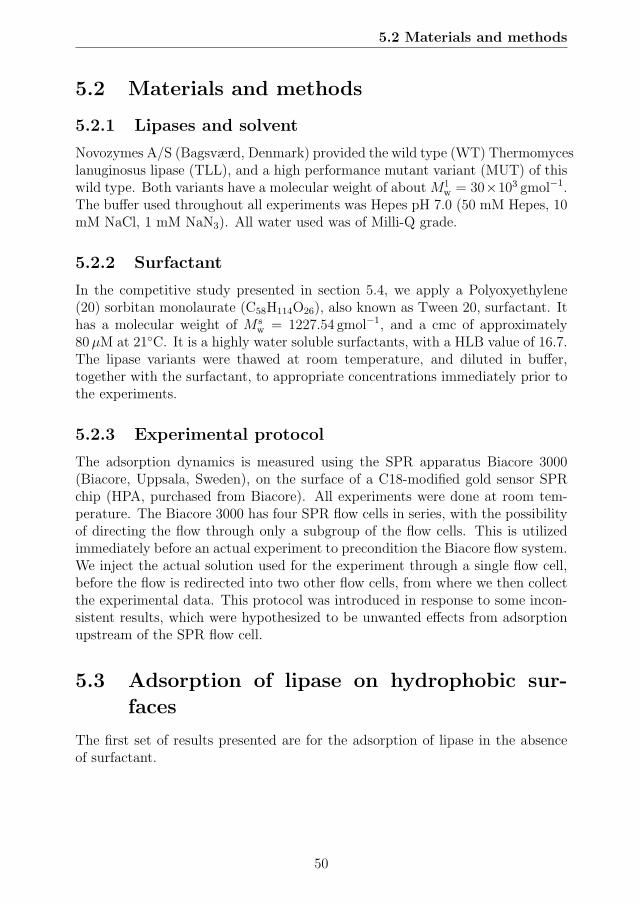
5.2 Materials and methods
5.2 Materials and methods
5.2.1 Lipases and solvent
Novozymes A/S (Bagsværd, Denmark) provided the wild type (WT) Thermomyceslanuginosus lipase (TLL), and a high performance mutant variant (MUT) of thiswild type. Both variants have a molecular weight of about M l
w = 30×103 gmol−1.The buffer used throughout all experiments was Hepes pH 7.0 (50 mM Hepes, 10mM NaCl, 1 mM NaN3). All water used was of Milli-Q grade.
5.2.2 Surfactant
In the competitive study presented in section 5.4, we apply a Polyoxyethylene(20) sorbitan monolaurate (C58H114O26), also known as Tween 20, surfactant. Ithas a molecular weight of M s
w = 1227.54 gmol−1, and a cmc of approximately80μM at 21◦C. It is a highly water soluble surfactants, with a HLB value of 16.7.The lipase variants were thawed at room temperature, and diluted in buffer,together with the surfactant, to appropriate concentrations immediately prior tothe experiments.
5.2.3 Experimental protocol
The adsorption dynamics is measured using the SPR apparatus Biacore 3000(Biacore, Uppsala, Sweden), on the surface of a C18-modified gold sensor SPRchip (HPA, purchased from Biacore). All experiments were done at room tem-perature. The Biacore 3000 has four SPR flow cells in series, with the possibilityof directing the flow through only a subgroup of the flow cells. This is utilizedimmediately before an actual experiment to precondition the Biacore flow system.We inject the actual solution used for the experiment through a single flow cell,before the flow is redirected into two other flow cells, from where we then collectthe experimental data. This protocol was introduced in response to some incon-sistent results, which were hypothesized to be unwanted effects from adsorptionupstream of the SPR flow cell.
5.3 Adsorption of lipase on hydrophobic sur-
faces
The first set of results presented are for the adsorption of lipase in the absenceof surfactant.
50
62

5.3 Adsorption of lipase on hydrophobic surfaces
5.3.1 Presentation and discussion of data
The first set of experiments presented is an investigation of the adsorption dy-namics of the two lipase variants introduced in section 5.2, in the absence of sur-factants. The main purposes of these experiments were to get data on adsorptiondynamics, upon which theoretical analysis could be based, and to qualitativelycompare the two lipase variants under different conditions. The experiments weredone under variation of injection flow rate and lipase concentration. The totalvolume of the injected solution was conserved at 150μL across all the experi-ments. Data is presented for two different flow rates, namely 5μLmin−1 and10μLmin−1, amounting to a total contact time of respectively 30min = 1800 sand 15min = 900 s. The two flow rates correspond to Peclet numbers (see sec-tion 3.3.2) of respectively Pe = 2500 and Pe = 5000. The six different injectionconcentrations were chosen as c0 ∈ {100, 150, 200, 300, 400, 500} nM. Two repeti-tions were done for a particular combination of parameters, and the mean valueis presented along with error bars based on the standard deviation of the two rep-etitions. Error bars are only showed at a subset of the times of recorded data toachieve a more clear presentation. Fig. 5.2 presents timeseries of the adsorptionprocess, i.e. the adsorbed amount Γ in [μgm−2] as a function of time. Fig. 5.3presents the data in the phase plane spanned by the adsorbed amount Γ and itstemporal rate of change dΓ/dt.
A universal behavior for all the data is that the adsorption rate, as wellas the saturation level, increases with injection concentration c0. The data issmooth and generally shows a monotone dependence of concentration and flowrate. In addition, the error bars are relatively small, indicating robust results atleast within the experimental run of all the parameter combinations. The phaseplane provides the clearest picture of the qualitative nature of the adsorptiondynamics. The adsorption dynamics of the wild type lipase, at the low Pecletnumber Pe = 2500 (Fig. 5.3 (a)), is close to linear for all concentrations. Asthe flow rate is increased (Fig. 5.3 (b)) the adsorption rates are increased muchmore drastically than expected from both quasi-steady theory and simulationsas presented in the preceding chapters. Quasi-steady theory predicts that themaximum adsorption rate scales with Pe1/3 (see Eq. (3.44)), in the convection-diffusion-limited regime, which is where the largest effect of flow rate occurs. Themuch more pronounced effect of flow rate in the experimental data asks for otherexplanations than those provided in the theoretical and numerical section of thisthesis. The wild type data at the high flow rate in Fig. 5.3 (b) also shows a moreconvex form, especially at high concentrations. This amounts to a prolongedadsorption to higher saturation levels than expected from a linear extrapolationof data at intermediate times. The phase plane dynamics of the mutant lipase in
51
63

5.3 Adsorption of lipase on hydrophobic surfaces
0 500 1000 1500 20000
200
400
600
800
1000
1200
(a) wild type, Pe=2500
time [s]
Γ [μ
gm−
2 ]
100 nM
150 nM
200 nM
300 nM
400 nM
500 nM
0 500 10000
200
400
600
800
1000
1200
(b) wild type, Pe=5000
time [s]
Γ [μ
gm−
2 ]
100 nM
150 nM
200 nM300 nM
400 nM500 nM
0 500 1000 1500 20000
500
1000
1500
2000
(c) mutant, Pe=2500
time [s]
Γ [μ
gm−
2 ]
100 nM
150 nM
200 nM
300 nM400 nM500 nM
0 500 10000
500
1000
1500
2000
(d) mutant, Pe=5000
time [s]
Γ [μ
gm−
2 ]
100 nM
150 nM
200 nM
400 nM300 nM500 nM
Figure 5.2: Timeseries obtained from SPR spectroscopy - wild type (a,b)and mutant (c,d) lipase for the flow rates 5μLmin−1 and 10μLmin−1.
Fig. 5.3 (c) and (d) has a more concave form for both flow rates. However, closeto saturation a small convex tail is also observed for the mutant. The increasein adsorption rate going from low to high flow rate is equally pronounced for themutant.
5.3.2 Inconsistency with expected behavior
Prior investigation of the lipase adsorption shows that the binding is irreversible,such that kd = 0. Therefore it is unexpected that the saturation levels dependon injection concentration. In other words, for irreversible adsorption the ex-pectation is an adsorption process up to some saturation level, which is ideallyindependent of bulk concentration, as long as there are enough bulk particles
52
64

5.3 Adsorption of lipase on hydrophobic surfaces
0 500 10000
1
2
3
4
5
6
7(a) wild type, Pe=2500
Γ [μgm−2]
dΓ/d
t [μ
gm−
2 s−1 ]
100 nM
150 nM
200 nM
300 nM
400 nM
500 nM
0 500 1000 15000
5
10
15
20
25(d) mutant, Pe=5000
Γ [μgm−2]
dΓ/d
t [μ
gm−
2 s−1 ]
100 nM150 nM
200 nM
300 nM
400 nM500 nM
0 500 1000 15000
1
2
3
4
5
6
7(c) mutant, Pe=2500
Γ [μgm−2]
dΓ/d
t [μ
gm−
2 s−1 ]
100 nM
150 nM
200 nM
300 nM
400 nM
500 nM
0 500 10000
5
10
15
20
25(b) wild type, Pe=5000
Γ [μgm−2]
dΓ/d
t [μ
gm−
2 s−1 ]
100 nM 150 nM
200 nM
300 nM
400 nM
500 nM
Figure 5.3: Phase plane representation of data from Fig. 5.2 - wild type(a,b) and mutant (c,d) lipase for the flow rates 5μLmin−1 and 10μLmin−1.
available for adsorption. This suggests that the injection plug, in some way, runsout of lipase as time progresses in the adsorption experiment. This inconsistencywas investigated further by running experiments with two consecutive injectionsof the mutant lipase. The concentration for the two consecutive injections wasfixed at values c0 ∈ {100, 200, 400} nM, and the flow rate was varied between25μLmin−1 and 100μLmin−1. The results of these experiments are presented inFig. 5.4. An increased adsorption is observed as the second injection is provided,which is more pronounced the lower the concentration gets. This suggests thatthe spatio-temporal profile of the injected concentration in the inlet of the flowcell, usually referred to as the injection plug, has a different nature than expectedfrom the interface with the Biacore SPR apparatus.
53
65
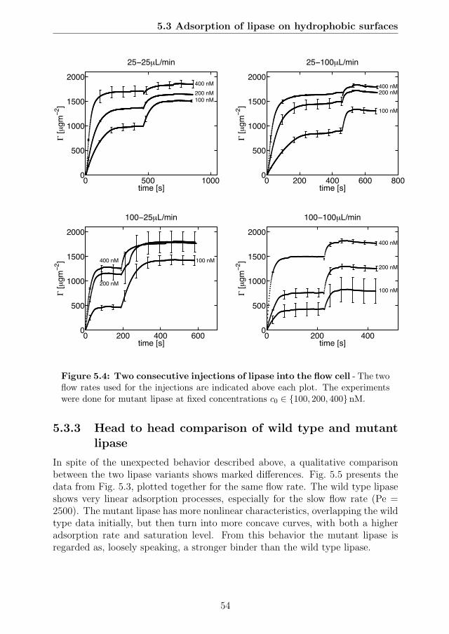
5.3 Adsorption of lipase on hydrophobic surfaces
0 500 10000
500
1000
1500
2000
time [s]
Γ [μ
gm−
2 ]25−25μL/min
100 nM200 nM
400 nM
0 200 400 600 8000
500
1000
1500
2000
time [s]
Γ [μ
gm−
2 ]
25−100μL/min
100 nM
200 nM400 nM
0 200 400 6000
500
1000
1500
2000
time [s]
Γ [μ
gm−
2 ]
100−25μL/min
100 nM
200 nM
400 nM
0 200 4000
500
1000
1500
2000
time [s]
Γ [μ
gm−
2 ]
100−100μL/min
100 nM
200 nM
400 nM
Figure 5.4: Two consecutive injections of lipase into the flow cell - The twoflow rates used for the injections are indicated above each plot. The experimentswere done for mutant lipase at fixed concentrations c0 ∈ {100, 200, 400} nM.
5.3.3 Head to head comparison of wild type and mutantlipase
In spite of the unexpected behavior described above, a qualitative comparisonbetween the two lipase variants shows marked differences. Fig. 5.5 presents thedata from Fig. 5.3, plotted together for the same flow rate. The wild type lipaseshows very linear adsorption processes, especially for the slow flow rate (Pe =2500). The mutant lipase has more nonlinear characteristics, overlapping the wildtype data initially, but then turn into more concave curves, with both a higheradsorption rate and saturation level. From this behavior the mutant lipase isregarded as, loosely speaking, a stronger binder than the wild type lipase.
54
66

5.3 Adsorption of lipase on hydrophobic surfaces
0 500 1000 15000
1
2
3
4
5
6
7
Γ [μgm−2]
dΓ/d
t [μ
gm−
2 s−1 ]
a) Pe=2500
wild typemutant
0 500 1000 15000
5
10
15
20
25
Γ [μgm−2]
dΓ/d
t [μ
gm−
2 s−1 ]
b) Pe=5000
wild typemutant
Figure 5.5: Head to head comparison of wild type and mutant lipase -Same data as in Fig. 5.2 and Fig. 5.3. (a) Flow rate: 5μLmin−1. (b) Flow rate:10μLmin−1. The concentrations are c0 ∈ {100, 150, 200, 300, 400, 500}nM.
5.3.4 Lipase adsorption rate constants
A crude estimation of the adsorption rate constants for the lipase data are ob-tained from the initial data. The convection-diffusion limitation is initially ne-glected such that, according to Eq. (3.5), the initial SPR response is given by
Γ(t = 0)model = kac0γm (5.1)
This model predicts a finite initial adsorption rate, in contrast with the experi-ments. However, in the limit of kinetically limited dynamics, we know from theresults in chapter 4, that the finite initial adsorption rate is close to the maximumadsorption rate in the experiment. Hence, setting Γ(t = 0)model = max(Γ)data,and using the maximum SPR response for the surface capacity for lipase γm, weobtain
ka =max(Γ)datac0max(Γ)
(5.2)
The adsorption rate constants for the wild type and mutant lipase, based onEq. (5.2), are presented in Fig. 5.6 and table 5.1. Interestingly, the estimatedadsorption rate constant are quite independent of the injection concentration.The estimated adsorption rate constants for the wild type are larger than for themutant for both Peclet numbers. Also, the estimated adsorption rate constantsincrease substantially with Peclet number, which is of course undesirable. Thisbehavior is consistent with the dramatic increase in adsorption rate under increasein flow rate mentioned above. Further theoretical analysis of the data, including
55
67

5.4 Competitive adsorption of lipase and surfactant
100 200 300 400 5000
0.5
1
1.5
2
2.5
3x 10⁴
Concentration c0 [nM]
k a [M−
1 s−1 ]
Pe=2500
WTMUT
100 200 300 400 5001
2
3
4
5
6
7
8x 10⁴
Concentration c0 [nM]
k a [M−
1 s−1 ]
Pe=5000
WTMUT
Figure 5.6: Lipase adsorption rate constants for the six concentrations- obtained from the initial data in Fig. 5.6 using Eq. (5.2)
Table 5.1: Lipase adsorption rate constants obtained from the initial data inFig. 5.6 using Eq. (5.2), given as mean values and standard deviation across thesix concentrations.
Pe = 2500 Pe = 5000kwta × 10−4 [M−1s−1] 1.1± 0.1 4.9± 0.6
kmuta × 10−4 [M−1s−1] 0.7± 0.2 3.2± 0.6
mass transport modeling, is not pursued, due to the apparent shortcoming ofinformation about the injection and operating conditions.
5.4 Competitive adsorption of lipase and sur-
factant
This section is concerned with competitive adsorption of lipase and surfactant.The study is in an early stage, and the scope of this section is merely to outlineour approach to the subject.
5.4.1 Identification of competitive regime
The outcome of the competitive process of lipase and surfactant adsorption de-pends on the relative concentrations of the two interacting species. Loosely speak-ing, if one of the species is overly outnumbered by the other, it gets no footholdon the surface. The primary scope of the study is the competitive adsorption
56
68
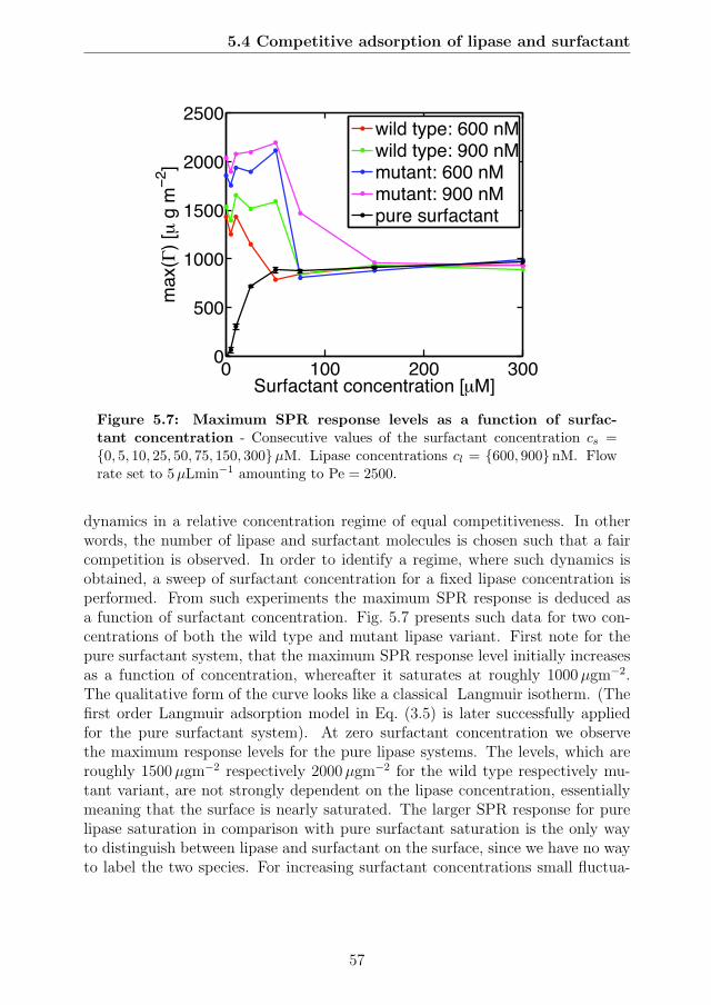
5.4 Competitive adsorption of lipase and surfactant
Figure 5.7: Maximum SPR response levels as a function of surfac-tant concentration - Consecutive values of the surfactant concentration cs ={0, 5, 10, 25, 50, 75, 150, 300}μM. Lipase concentrations cl = {600, 900}nM. Flowrate set to 5μLmin−1 amounting to Pe = 2500.
dynamics in a relative concentration regime of equal competitiveness. In otherwords, the number of lipase and surfactant molecules is chosen such that a faircompetition is observed. In order to identify a regime, where such dynamics isobtained, a sweep of surfactant concentration for a fixed lipase concentration isperformed. From such experiments the maximum SPR response is deduced asa function of surfactant concentration. Fig. 5.7 presents such data for two con-centrations of both the wild type and mutant lipase variant. First note for thepure surfactant system, that the maximum SPR response level initially increasesas a function of concentration, whereafter it saturates at roughly 1000μgm−2.The qualitative form of the curve looks like a classical Langmuir isotherm. (Thefirst order Langmuir adsorption model in Eq. (3.5) is later successfully appliedfor the pure surfactant system). At zero surfactant concentration we observethe maximum response levels for the pure lipase systems. The levels, which areroughly 1500μgm−2 respectively 2000μgm−2 for the wild type respectively mu-tant variant, are not strongly dependent on the lipase concentration, essentiallymeaning that the surface is nearly saturated. The larger SPR response for purelipase saturation in comparison with pure surfactant saturation is the only wayto distinguish between lipase and surfactant on the surface, since we have no wayto label the two species. For increasing surfactant concentrations small fluctua-
57
69

5.4 Competitive adsorption of lipase and surfactant
tions in the maximum response are observed first. There is, however, a trend ofa minor increase in the SPR response as a function of surfactant concentration,which suggests that surfactant and lipase are present on the surface together insome kind of optimal mixed state. This regime is followed by a steep decrease inthe response towards the pure surfactant response. Importantly, this steep de-crease is displaced towards higher surfactant concentrations for increasing lipaseconcentration, supporting that the desired competitive regime is determined. Athigh surfactant concentration, i.e. above 150μM the surfactant system is totallydominant in the competitive process. The regime where the surfactant beginsto dominate is closely related to the cmc of the surfactant, which for aqueoussolution at ambient temperature is around 80μM. This value, however, naturallydepends on the solvent medium and the presence of other solutes. The data showsa rather smooth concentration dependency, i.e. no abrupt or singular behavioris observed. One could therefore conclude from the regime at around surfactantconcentrations of 0−100μM, that increasing the surfactant concentration simplyleads to larger fraction of the surface it occupies in equilibrium. One must, how-ever, keep in mind that the data in Fig. 5.7 are maximum response levels, and notequilibrium levels. As seen below the dynamical adsorption process shows first aquick increase, and then a slow decrease, in the SPR signal as a function of time,supporting that maximum response levels in Fig. 5.7 are not isotherms, and nota measure of equilibrium. As seen below the process is also greatly influencedby the flow rate, which was set to 5μLmin−1 amounting to Pe = 2500 for theexperiments in Fig. 5.7. This experiment primarily serves to identify some lipaseand surfactant concentrations, at which we then put focus on the underlyingdynamical adsorption process.
5.4.2 The competitive adsorption dynamics of lipase andsurfactant
Based on the preliminary experimental results, presented above in Fig. 5.7, wemove on to study the competitive adsorption dynamics of lipase and surfactantfor both wild type and mutant lipase. The lipase concentration was chosen ascl = 800 nM, and the surfactant concentration was chosen as cs = 50μM. Thedynamical adsorption process was then obtained, using both wild type and mu-tant lipase. The adsorption experiments were run at two different flow rates,5μLmin−1 and 20μLmin−1. The two flow rates amounts to Pe = {2500, 10000}.The total volume of solution injected in the association phase was 150μL for bothflow rates, which implies that the duration of the association phase was 30min and7.5min, respectively. An association phase was directly followed by a dissociationphase of pure buffer injection to obtain ideal conditions for probing desorption
58
70
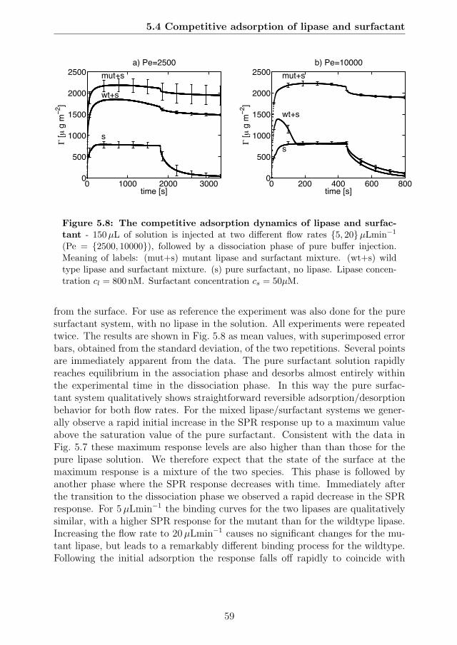
5.4 Competitive adsorption of lipase and surfactant
0 1000 2000 30000
500
1000
1500
2000
2500a) Pe=2500
time [s]
Γ [μ
g m
−2 ]
s
wt+s
mut+s
0 200 400 600 8000
500
1000
1500
2000
2500b) Pe=10000
time [s]
Γ [μ
g m
−2 ]
s
wt+s
mut+s
Figure 5.8: The competitive adsorption dynamics of lipase and surfac-tant - 150μL of solution is injected at two different flow rates {5, 20}μLmin−1
(Pe = {2500, 10000}), followed by a dissociation phase of pure buffer injection.Meaning of labels: (mut+s) mutant lipase and surfactant mixture. (wt+s) wildtype lipase and surfactant mixture. (s) pure surfactant, no lipase. Lipase concen-tration cl = 800 nM. Surfactant concentration cs = 50μM.
from the surface. For use as reference the experiment was also done for the puresurfactant system, with no lipase in the solution. All experiments were repeatedtwice. The results are shown in Fig. 5.8 as mean values, with superimposed errorbars, obtained from the standard deviation, of the two repetitions. Several pointsare immediately apparent from the data. The pure surfactant solution rapidlyreaches equilibrium in the association phase and desorbs almost entirely withinthe experimental time in the dissociation phase. In this way the pure surfac-tant system qualitatively shows straightforward reversible adsorption/desorptionbehavior for both flow rates. For the mixed lipase/surfactant systems we gener-ally observe a rapid initial increase in the SPR response up to a maximum valueabove the saturation value of the pure surfactant. Consistent with the data inFig. 5.7 these maximum response levels are also higher than than those for thepure lipase solution. We therefore expect that the state of the surface at themaximum response is a mixture of the two species. This phase is followed byanother phase where the SPR response decreases with time. Immediately afterthe transition to the dissociation phase we observed a rapid decrease in the SPRresponse. For 5μLmin−1 the binding curves for the two lipases are qualitativelysimilar, with a higher SPR response for the mutant than for the wildtype lipase.Increasing the flow rate to 20μLmin−1 causes no significant changes for the mu-tant lipase, but leads to a remarkably different binding process for the wildtype.Following the initial adsorption the response falls off rapidly to coincide with
59
71

5.4 Competitive adsorption of lipase and surfactant
the response for the pure surfactant solution. For all lipase/surfactant data, butthe wild type at Pe = 10000, the decrease following the maximum response isrelatively slow, and the following desorption in the dissociation phase is limited(partly irreversible). For the wild type lipase/surfactant system at Pe = 10000the decrease in the signal, after the maximum response, is so rapid that the dataessentially follows those for the pure surfactant system from an early time beforethe dissociation phase. In the dissociation phase we observe reversible desorption.
We do not know if a longer association phase would lead to data for the mixedsystems, which would eventually coincide with the data for the pure surfactantsystem, for all the experiments. From the data shown in Fig. 5.8, we can onlyhypothesize about the potential progress of the dynamics if the dissociation phasewas shifted to a later start. A head to head comparison of the two lipase variantsshows that the mutant adsorbs to higher response levels. This is expected tobe caused by a closer packing on the surface, stemming from a lesser degree ofintermolecular repulsion between the lipases. Also, the mutant seems strongerin relation to the competition with surfactant, especially at the higher flow rate(Pe = 10000), where the wild type lipase gets almost no foothold in the compe-tition whatsoever.
With the goal of getting a better comparison between the two different flowrates in Fig. 5.8, we plot the SPR response as a function of injected amount,instead of as a function of time. In this way, all the data can be combinedinto a single plot. The error bars are omitted, and the mean values are pre-sented in Fig. 5.9. The general shape of the pure surfactant data, as well asthe mutant/surfactant data, is conserved across change in flow rate. The wildtype/surfactant data, however, clearly shows that the increase in flow rate dras-tically favors the surfactant above the lipase competitiveness. This suggests thatthe rate of arrival, which is increased by an increased flow rate, is critical in thecompetitive process. A direct hydrodynamic effect is not expected to be impor-tant, due to the very low flow rates close to the surface, and around particleswith sizes in the order of nanometers. Fig. 5.9 also shows a small decrease inthe initial SPR response, as a function of injected amount, when the flow rate isincreased. This is a characteristic of a kinetically limited process, where a fasterinjection implies that more solution flows past the sensor surface, without gettingadsorbed.
5.4.3 Surfactant dynamics from Langmuir adsorption model
As a first quantitative approach to the data, we fit the first order Langmuirmodel in Eq. 3.5 to the pure surfactant dynamics. In this way we initially neglect
60
72

5.4 Competitive adsorption of lipase and surfactant
Figure 5.9: The data from Fig 5.8 combined into a single plot as a func-tion of injected amount. - Association phase consisting of a 150μL injection,followed by dissociation phase of pure buffer injection. Meaning of labels: (mut+s)mutant lipase and surfactant mixture. (wt+s) wild type lipase and surfactant mix-ture. (s) pure surfactant, no lipase. Lipase concentration cl = 800 nM. Surfactantconcentration cs = 50μM.
convection-diffusion limitation. The bulk concentration is set to cs = 50μM. Theresults of nonlinear least squares fitting, for both 5μLmin−1 and 20μLmin−1,are presented in Fig. 5.10, and the obtained fitting parameters are presentedin Table 5.2. The overall quality of both fits looks reasonably good. The ob-tained adsorption rate constant ka,s slightly increases with Peclet number, butwith a minor difference of about 6 percent. The desorption rate constant kd,sincreases more substantially with Peclet number, and since the saturation valueis almost the same for the two Peclet numbers, the larger desorption rate con-stant is compensated for by a larger value of the maximum surface capacity γm,s.Corresponding Damkohler and Biot numbers are also given in Table 5.2. Thenumerically low values support that the dynamics is in the regime of kineticlimitation, such that convection-diffusion limitation can be neglected, withoutimposing significant errors on the result.
61
73

5.4 Competitive adsorption of lipase and surfactant
0 200 400 600 8000
200
400
600
800
1000Pe=10000
time [s]
Γ [μ
g m
−2 ]
surfactant dataLangmuir model
0 1000 2000 30000
200
400
600
800
1000Pe=2500
time [s]
Γ [μ
g m
−2 ]
surfactant dataLangmuir model
Figure 5.10: Fit of the Langmuir model (Eq. 3.5) to surfactant data -The obtained parameters are presented in table 5.2.
Table 5.2: Surfactant parameters obtained from the fit shown in Fig. 5.10.
Pe = 2500 Pe = 10000ka,s [M
−1s−1] 772 823kd,s [s
−1] 0.00386 0.00867γm,s [μgm
−2] 821 980Da 3.00× 10⁻⁴ 2.40× 10⁻⁴
Bi 0.0023 0.0029
5.4.4 Lipase adsorption rate constants
A crude estimation of the adsorption rate constants for the lipase data can bedone from the initial data. Again, the convection-diffusion limitation is initiallyneglected. According to Eqs. (3.24) and Eq. (3.4) this assumption implies aninitial SPR response given by
Γ(t = 0)model = ka,eceγm,e + ka,scsγm,s (5.3)
This model predicts a finite initial adsorption rate, in contrast with the experi-ments. However, in the limit of kinetically limited dynamics, we know from theresults in chapter 4, that the finite initial adsorption rate is close to the maximumadsorption rate in the experiment. Hence, setting Γ(t = 0)model = max(Γ)data,using the surfactant parameters from table 5.2, and estimating the maximumsurface capacity for lipase γm,e from the maximum SPR response, we put
ka,e =max(Γ)data − ka,scsγm,s
cemax(Γ)(5.4)
62
74

5.4 Competitive adsorption of lipase and surfactant
Table 5.3: Lipase adsorption rate constants obtained from the initial data inFig. 5.8 using Eq. (5.4).
Pe = 2500 Pe = 10000kwta,l × 10−4 [M−1s−1] 10.2 9.3
kmuta,l × 10−4 [M−1s−1] 8.2 13.2
Estimates for the adsorption rate constants for the wild type and mutant lipase,based on the competitive data in Fig. 5.8 and Eq. (5.4), are presented in table 5.3.The lipase adsorption rate constants in the presence of surfactants are about oneorder of magnitude larger than those obtained in the absence of surfactants intable 5.1. One hypothesis to explain this increase is that surfactant moleculesscreen lipase adsorption downstream of the SPR chip, which could lead to a higheractual lipase concentration available at the location of the SPR measurement.
5.4.5 Problems with reproducibility
The presented data on competitive adsorption of lipase and surfactants hintsat some rich dynamics, as well as intriguing flow rate dependencies. However,following the measurements presented above, we encountered problems with re-producibility of the data. New data showed different, and less dramatic, behavior.The observations included a lesser degree of apparent displacement of lipase bysurfactant, as well as a much less dramatic flow rate dependency. However, theresponse obtained for the pure surfactant system was substantially lower than forthe data presented above, questioning the quality of the data. The collection ofdisconcerting results was continued until the Biacore SPR apparatus developed afailure so severe that the system shut down, and subsequent assistance from GEHealthcare (producers of Biacore) was required. This is the current status of thework, and further experimental investigations are therefore beyond the scope ofthe present dissertation. By the same token, further theoretical investigations,including an attempt of applying the bimolecular theory from section 3.4 to thedata, needs stronger experimental support. Possible future work is discussed inchapter 6.
63
75

76

Chapter 6
Concluding remarks
6.1 Conclusions
The thesis brought different aspects of surface-based biosensors, and in particu-lar SPR spectroscopy, into focus. Following a somewhat general review of SPRspectroscopy, including relevant applications, the theoretical framework for masstransport dynamics was developed in detail. Kinetic and diffusion scalings oftime lead to nondimensional formulations that provide users of the surface-basedbiosensor technologies with a correct set of parameters to characterize the operat-ing regime for their experiments. The widely adopted quasi-steady theory, whichusers of the technologies often employ in order to avoid cumbersome numericalsolutions of the entire transport problem, was analyzed in detail. In this respect,the parameterization of the quasi-steady theory was related to the more compre-hensive parameterization of the entire transport problem. The numerical resultsin the thesis yielded a way to correct experimentally obtained adsorption rateconstants, based on fitting data with the quasi-steady theory. The problem ofsolute adsorption to all surfaces in the biosensor flow cell, besides the sensor sur-face, was briefly investigated numerically. Adsorption of a wild type and mutantlipase to a model hydrophobic surface, as well as competitive adsorption of lipaseand surfactant, was investigated by a Biacore SPR reader. Qualitative compari-son of the wild type and the mutant lipase showed higher saturation levels, andstronger competitiveness against surfactant, for the mutant. Adsorption and des-orption rate constants for the studied species were estimated from the data. Weemphasized some experimental conditions, which should be met in order for theexperiments to form basis for rigorous theoretical modeling.
65
77

6.2 Future perspective
6.2 Future perspective
In this section some of the most natural future work is discussed. Surely, thereare other possibilities, since the suggestions are naturally biased towards someof the issues which have had primary focus during the project. The sectionis divided into suggestions of a purely theoretical nature, then suggestions ofa purely experimental nature, and finally, possible future work in the interfacebetween theory and experiments.
6.2.1 Future theoretical work
• From a theoretical viewpoint a boundary layer theory, for which the quasi-steady theory is a first order approximation, is an interesting goal. Sucha theoretical development could deepen the fundamental understanding ofthe quasi-steady theory, and furthermore suggest corrections to the modelto better capture the convection-diffusion-limited regime. Such work couldperhaps even be developed for other geometries encountered in other kindsof surface-based biosensors, as well as technological and natural systemsmore generally.
• Another issue, which could be analyzed in more detail than done in this the-sis, is the effect of adsorption to surfaces besides the sensor surface. Thiswork asks for a more thorough parameter study. A similar study for thebimolecular system, which encompass an even larger undiscovered parame-ter space, could be done. This study forms an interesting theoretical modelbasis for investigations of the possibility of screening unwanted adsorptionof one specie by adsorption of another specie in the same solution.
• The theoretical framework developed for the bimolecular system can beused to determine parameter regimes where a two-component quasi-steadytheory, and even just pure kinetic models, have sufficient accuracy for datafitting. This work could follow the progress of the manuscript [P1], butnaturally involves a more extensive parameter investigation.
6.2.2 Future experimental work
• The previous suggestion of a model system for studying the possibility ofscreening unwanted adsorption is connected to a hypothesis on the exper-imental system. Namely, that the larger lipase adsorption rate constants,obtained for the experimental system including surfactant, can be explainedby a larger bulk concentration of lipase due to screening of unwanted up-stream adsorption of lipase by the surfactant. Support for this interpre-
66
78
6.2 Future perspective
tation could be searched for by experimental investigations using differentrelative concentrations of lipase and surfactants, and also different molecu-lar species.
• More importantly, a major milestone is to obtain adsorption profiles forpure lipase solutions with concentration independent saturation. This goalshould be theoretically possible for the concentrations used in this thesis,yet we observe steady-state at surface coverage levels below saturation. Theexperimental study with two consecutive injections of lipase suggest that theinjection conditions are practically unknown. An experimental resolutionof this issue should have top priority.
6.2.3 Future work in the interface between theory andexperiments
• A more thorough link between theoretical models and experiments is anatural goal for the future. The simple first order model, as well as thesuggested competitive model in section 3.4 can be applied to a more com-prehensive set of data, and the competition parameters could be estimated.The competition parameters would then characterize a given system, andthey could be used as quantifiers across different flow rates and relativeconcentrations. Concerning the competitive adsorption study outlined inthe thesis, a theoretical model that takes into account the dynamics of mi-celle formation, and the adsorption/desorption dynamics of single surfac-tant molecules and micelles separately, could be a future goal. This wouldbe an interesting model system for theoretical investigations, and broughtto a higher impact level by combining it with supporting experiments.
67
79

80
References
Aguilar, M.I. and Small, D.H. (2005). Surface plasmon resonance for the analysis ofbeta-amyloid interactions and fibril formation in alzheimer’s disease research. Neu-rotox Res, 7(1-2):17–27. 11
Alvarez, N.J., Walker, L.M. and Anna, S.L. (2010). Diffusion-limited adsorption toa spherical geometry: The impact of curvature and competitive time scales. Phys.Rev. E, 82:011604. 18
Anderluh, G., Macek, P. and Lakey, J.H. (2003). Peeking into a secret world of pore-forming toxins: membrane binding processes studied by surface plasmon resonance.Toxicon, 42(3):225–8. 11
Bakrac, B., Gutierrez-Aguirre, I., Podlesek, Z., Sonnen, A.F.P., Gilbert, R.J.C., Macek,P., Lakey, J.H. and Anderluh, G. (2008). Molecular determinants of sphingomyelinspecificity of a eukaryotic pore-forming toxin. J Biol Chem, 283(27):18665–77. 11
Batchelor, G.K. (1967). An introduction to fluid dynamics. U.P., Cambridge. 14
Besenicar, M., Macek, P., Lakey, J.H. and Anderluh, G. (2006). Surface plasmonresonance in protein-membrane interactions. Chem Phys Lipids, 141(1-2):169–78. 5,9, 10, 11
Besenicar, M.P. and Anderluh, G. (2010). Preparation of lipid membrane surfaces formolecular interaction studies by surface plasmon resonance biosensors. Methods MolBiol, 627:191–200. 11
Bird, R.B., Stewart, W.E. and Lightfoot, E.N. (2002). Transport phenomena. J. Wiley,New York, 2nd, wiley international ed edition. 33, 35, 36
Brody, J.P., Yager, P., Goldstein, R.E. and Austin, R.H. (1996). Biotechnology at lowreynolds numbers. Biophys J, 71(6):3430–41. 14
Brzozowski, A.M., Savage, H., Verma, C.S., Turkenburg, J.P., Lawson, D.M., Svend-sen, A. and Patkar, S. (2000). Structural origins of the interfacial activation inthermomyces (humicola) lanuginosa lipase. Biochemistry, 39(49):15071–82. 48
69
81

REFERENCES
Bunjes, N., Schmidt, E., Jonczyk, A., Rippmann, F., Beyer, D., Ringsdorf, H., Graber,P., Knoll, W. and Naumann, R. (1997). Thiopeptide-supported lipid layers on solidsubstrates. Langmuir, 13(23):6188–6194. 10
Cho, W., Bittova, L. and Stahelin, R.V. (2001). Membrane binding assays for peripheralproteins. Anal Biochem, 296(2):153–61. 11
Cooper, M.A., Hansson, A., Lofas, S. and Williams, D.H. (2000). A vesicle capturesensor chip for kinetic analysis of interactions with membrane-bound receptors. An-alytical Biochemistry, 277(2):196–205. 10
Cooper, M.A., Try, A.C., Carroll, J., Ellar, D.J. and Williams, D.H. (1998). Surfaceplasmon resonance analysis at a supported lipid monolayer. Biochim Biophys Acta,1373(1):101–11. 10
Cooper, M. (2004). Advances in membrane receptor screening and analysis. J. Mol.Recognit., 17(4):286–315. 10, 11
Cooper, M.A. (2002). Optical biosensors in drug discovery. Nat. Rev. Drug Disc.,1(7):515–28. 10
Cygler, M. and Schrag, J.D. (1997). Structure as basis for understanding interfacialproperties of lipases. Methods Enzymol, 284:3–27. 48
Duinhoven, S., Poort, R., der Voet, G.V., Agterof, W., Norde, W. and Lyklema, J.(1995). Driving forces for enzyme adsorption at solid-liquid interfaces: 1. the serineprotease savinase. Journal of Colloid and Interface Science, 170(2):340 – 350. 48
Fu, Z. and Santore, M.M. (1998). Kinetics of competitive adsorption of peo chains withdifferent molecular weights. Macromolecules, 31(20):7014–7022. 24
Gennes, P.G.d., Brochard-Wyart, F. and Quere, D. (2004). Capillarity and wettingphenomena: drops, bubbles, pearls, waves. Springer, New York. 48
Gervais, T. and Jensen, K.F. (2006). Mass transport and surface reactions in microflu-idic systems. Chemical Engineering Science, 61(4):1102 – 1121. 16
Goldstein, B., Coombs, D., He, X., Pineda, A.R. and Wofsy, C. (1999 Sep-Oct). Theinfluence of transport on the kinetics of binding to surface receptors: application tocells and biacore. J Mol Recognit, 12(5):293–299. 12
Goren, M., Galley, N. and Lennox, R.B. (2006 Jan 31). Adsorption of alkylthiol-capped gold nanoparticles onto alkylthiol self-assembled monolayers: an spr study.Langmuir, 22(3):1048–1054. 31, 37
Graneli, A., Edvardsson, M. and Hook, F. (2004). Dna-based formation of a supported,three-dimensional lipid vesicle matrix probed by qcm-d and spr. ChemPhysChem,5(5):729–33. 10
70
82

REFERENCES
Heyse, S., Ernst, O.P., Dienes, Z., Hofmann, K.P. and Vogel, H. (1998). Incorporationof rhodopsin in laterally structured supported membranes: observation of transducinactivation with spatially and time-resolved surface plasmon resonance. Biochemistry,37(2):507–22. 10, 11
Homola, J. (2008). Surface plasmon resonance sensors for detection of chemical andbiological species. Chem Rev, 108(2):462–93. 5, 6
Jones, J.A., Rawles, R. and Hannun, Y.A. (2005). Identification of a novel phosphatidicacid binding domain in protein phosphatase-1. Biochemistry, 44(40):13235–45. 11
Kodoyianni, V. (2011). Label-free analysis of biomolecular interactions using spr imag-ing. Biotech., 50(1):32–40. 9
Kuziemko, G.M., Stroh, M. and Stevens, R.C. (1996). Cholera toxin binding affinity andspecificity for gangliosides determined by surface plasmon resonance. Biochemistry,35(20):6375–84. 11
Lang, H., Duschl, C. and Vogel, H. (1994). A new class of thiolipids for the attachmentof lipid bilayers on gold surfaces. Langmuir, 10(1):197–210. 10
Maldonado-Valderrama, J., Wilde, P., Macierzanka, A. and Mackie, A. (2011). Therole of bile salts in digestion. Adv Colloid Interface Sci, 165(1):36–46. 48
Mason, T., Pineda, A.R., Wofsy, C. and Goldstein, B. (1999). Effective rate models forthe analysis of transport-dependent biosensor data. Math Biosci, 159(2):123–44. 12
Mogensen, J.E., Sehgal, P. and Otzen, D.E. (2005). Activation, inhibition, and destabi-lization of thermomyces lanuginosus lipase by detergents. Biochemistry, 44(5):1719–30. 48
Mouritsen, O.G. (2005). Life - as a matter of fat: the emerging science of lipidomics.Springer, Berlin. 47
Mozsolits, H., Thomas, W. and Aguilar, M. (2003). Surface plasmon resonance spec-troscopy in the study of membranemediated cell signalling. J. Peptide Sci., 9(2):77–89. 11
Mozsolits, H. and Aguilar, M.I. (2002). Surface plasmon resonance spectroscopy: anemerging tool for the study of peptide-membrane interactions. Biopolymers, 66(1):3–18. 11
Myszka, D.G., He, X., Dembo, M., Morton, T.A. and Goldstein, B. (1998 Aug). Extend-ing the range of rate constants available from biacore: interpreting mass transport-influenced binding data. Biophys J, 75(2):583–594. 11, 12, 31
71
83
REFERENCES
Myszka, D.G., Morton, T.A., Doyle, M.L. and Chaiken, I.M. (1997 Feb 28). Kineticanalysis of a protein antigen-antibody interaction limited by mass transport on anoptical biosensor. Biophys Chem, 64(1-3):127–137. 31
Noinville, S., Vidic, J. and Dejardin, P. (2010). Adsorption rate dependence on convec-tion over a large length of a sensor to get adsorption constant and solute diffusioncoefficient. Colloids Surf B Biointerfaces, 76(1):112–6. 12
Piliarik, M., Vaisocherova, H. and Homola, J. (2009). Surface plasmon resonancebiosensing. Methods Mol Biol, 503:65–88. 6, 7, 8, 9
Pinholt, C., Fanø, M., Wiberg, C., Hostrup, S., Bukrinsky, J.T., Frokjaer, S., Norde,W. and Jorgensen, L. (2010). Influence of glycosylation on the adsorption of ther-momyces lanuginosus lipase to hydrophobic and hydrophilic surfaces. Eur J PharmSci, 40(4):273–81. 48
Plant, A. (1993). Self-assembled phospholipid/alkanethiol biomimetic bilayers on gold.Langmuir, 9(11):2764–2767. 10
Plant, A., Brighamburke, M., Petrella, E. and Oshannessy, D. (1995). Phospho-lipid/alkanethiol bilayers for cell-surface receptor studies by surface plasmon res-onance. Analytical Biochemistry, 226(2):342–348. 10
Raether, H. (1997). Surface plasmons on smooth and rough surfaces and on gratings.Springer Tracts in Modern Physics (Springer, Berlin, 1988). 7
Reis, P., Holmberg, K., Watzke, H., Leser, M.E. and Miller, R. (2009). Lipases atinterfaces: a review. Adv Colloid Interface Sci, 147-148:237–50. 48
Rich, R.L. and Myszka, D.G. (2007). Survey of the year 2006 commercial opticalbiosensor literature. J Mol Recognit, 20(5):300–66. 12
Rich, R.L. and Myszka, D.G. (2008). Survey of the year 2007 commercial opticalbiosensor literature. J Mol Recognit, 21(6):355–400. 12
Rich, R.L. and Myszka, D.G. (2010). Grading the commercial optical biosensorliterature-class of 2008: ’the mighty binders’. J Mol Recognit, 23(1):1–64. 12
Robelek, R. (2009). Surface plasmon resonance sensors in cell biology: basics andapplication. Bioanal Rev, 1(1):57–72. 9
Saenko, E., Sarafanov, A., Ananyeva, N., Behre, E., Shima, M., Schwinn, H. and Josic,D. (2001). Comparison of the properties of phospholipid surfaces formed on hpa andl1 biosensor chips for the binding of the coagulation factor viii. J Chromatogr A,921(1):49–56. 11
Salamon, Z., Brown, M. and Tollin, G. (1999). Plasmon resonance spectroscopy: prob-ing molecular interactions within membranes. Trends Biochem Sci, 24:213–219. 11
72
84
REFERENCES
Schmid, R.D. and Verger, R. (1998). Lipases: Interfacial enzymes with attractiveapplications. Angewandte Chemie International Edition, 37(12):1608–1633. 48
Schuck, P. (1996). Kinetics of ligand binding to receptor immobilized in a polymermatrix, as detected with an evanescent wave biosensor. i. a computer simulation ofthe influence of mass transport. Biophys J, 70(3):1230–49. 12
Schuck, P. and Minton, A.P. (1996). Analysis of mass transport-limited binding kineticsin evanescent wave biosensors. Anal Biochem, 240(2):262–72. 11, 12, 31
Sonesson, A.W., Blom, H., Hassler, K., Elofsson, U.M., Callisen, T.H., Widengren, J.and Brismar, H. (2008). Protein-surfactant interactions at hydrophobic interfacesstudied with total internal reflection fluorescence correlation spectroscopy (tir-fcs).J Colloid Interface Sci, 317(2):449–57. 48
Sonesson, A.W., Elofsson, U.M., Brismar, H. and Callisen, T.H. (2006). Adsorptionand mobility of a lipase at a hydrophobic surface in the presence of surfactants.Langmuir, 22(13):5810–7. 48
Squires, T.M., Messinger, R.J. and Manalis, S.R. (2008). Making it stick: convection,reaction and diffusion in surface-based biosensors. Nat Biotechnol, 26(4):417–26. 18
Stahelin, R.V. and Cho, W. (2001). Differential roles of ionic, aliphatic, and aromaticresidues in membrane-protein interactions: a surface plasmon resonance study onphospholipases a2. Biochemistry, 40(15):4672–8. 11
Stenberg, E., Persson, B., Roos, H. and Urbaniczky, C. (1991). Quantitative deter-mination of surface concentration of protein with surface plasmon resonance usingradiolabeled proteins. Journal of Colloid and Interface Science, 143(2):513 – 526. 8
Stora, T., Lakey, J. and Vogel, H. (1999). Ion-channel gating in transmembrane receptorproteins: functional activity in tethered lipid membranes. Angewandte Chemie-International Edition, 38(3):389–391. 10, 11
Terrettaz, S., Stora, T., Duschl, C. and Vogel, H. (1993). Protein binding to sup-ported lipid membranes: investigation of the cholera toxin-ganglioside interactionby simultaneous impedance spectroscopy and surface plasmon resonance. Langmuir,9(5):1361–1369. 10
Wahlgren, M. and Arnebrant, T. (1991). Protein adsorption to solid surfaces. TrendsBiotechnol, 9(6):201–8. 48
Wannerberger, K. and Arnebrant, T. (1996). Lipases from humicola lanuginosa ad-sorbed to hydrophobic surfaces–desorption and activity after addition of surfactants.Colloids and Surfaces B: Biointerfaces. 48
73
85

Wannerberger, K., Wahlgren, M. and Arnebrant, T. (1996). Adsorption from lipase-surfactant solutions onto methylated silica surfaces. Colloids and Surfaces B: . . . .48
Ward, L.D. and Winzor, D.J. (2000). Relative merits of optical biosensors based onflow-cell and cuvette designs. Analytical Biochemistry, 285(2):179–93. 8
Wilde, P.J. and Chu, B.S. (2011). Interfacial & colloidal aspects of lipid digestion. AdvColloid Interface Sci, 165(1):14–22. 48
74
86

[P1]
87

88
Transient Convection, Diffusion, and Adsorption in
Surface-based Biosensors
Rasmus Hansen,∗,† Henrik Bruus,‡ Thomas H. Callisen,¶ and Ole Hassager∗,†
Department of Chemical and Biochemical Engineering, Technical University of Denmark,
Department of Micro- and Nanotechnology, Technical University of Denmark, and Novozymes
A/S
E-mail: [email protected]; [email protected]
Abstract
This paper presents a theoretical and computational investigation of convection, diffusion,
and adsorption in surface-based biosensors. In particular, we study the transport dynamics
in a model geometry of a Biacore surface plasmon resonance (SPR) sensor. The work, how-
ever, is equally relevant for other microfluidic surface-based biosensors, operating under flow
conditions. A widely adopted approximate quasi-steady theory to capture convective and dif-
fusive mass transport is reviewed, and an analytical solution is presented. An expression of
the Damköhler number is derived in terms of the nondimensional adsorption coefficient (Biot
number), the nondimensional flow rate (Péclet number), and the model geometry. Transient
dynamics is investigated and we quantify the error of using the quasi-steady-state assump-
tion for experimental data fitting in both kinetically limited and convection-diffusion-limited
∗To whom correspondence should be addressed†Department of Chemical and Biochemical Engineering, Technical University of Denmark, DTU Chemical Engi-
neering Building 227, DK-2800 Kongens Lyngby, Denmark‡Department of Micro- and Nanotechnology, Technical University of Denmark, DTU Nanotech Building 345 B,
DK-2800 Kongens Lyngby, Denmark¶Novozymes A/S, Novo Allé, 2880 - Bagsværd, Denmark
1
89

regimes. The results clarify the conditions under which the quasi-steady theory is reliable or
not. In extension to the well known fact that the range of validity is altered under convection-
diffusion-limited conditions, we show how also the ratio of the inlet concentration to the max-
imum surface capacity is critical for reliable use of the quasi-steady theory. Finally, our results
provide users of surface-based biosensors with a tool of correcting experimentally obtained
adsorption rate constants.
Introduction
Surface-based biosensors are increasingly used to investigate adsorption dynamics of molecular
systems. Surface plasmon resonance (SPR) spectroscopy is a particular technique that is well es-
tablished as a surface-based biosensor, allowing label-free, real time monitoring of adsorption of
biological macromolecules, such as proteins. For a detailed description of the principles behind
SPR spectroscopy see Stenberg et al.,1 and for more recent reviews of SPR sensors see Homola
et al. 2 and Homola.3
While the SPR technique, developed and commercialized by e.g. Biacore, is well capable of
capturing qualitative behavior, quantitative studies of chemical rate constants and equilibrium con-
stants are more challenging. Inconsistencies in derived rate constants has lead to both experimental
and theoretical investigations of the effect of convection and diffusion on the SPR signal.4,5 Signifi-
cant progress was made by the application of a quasi-steady-state approximation, i.e. a steady-state
bulk mass transport coupled to a dynamic adsorption scheme (explained in details below). This
approximation has been widely adopted for Biacore data analysis.5–10 However, practice in the
biochemical society still, to a large degree, consists of empirical and qualitative studies.11–14
The quasi-steady-state approximation leads to a nondimensional number called the Damköhler
number, which is sometimes referred to as the limit coefficient. An expression of the Damköhler
number is derived in terms of the nondimensional adsorption coefficient (Biot number), the nondi-
2
90

mensional flow rate (Péclet number), and the model geometry. The ability of the quasi-steady
theory to capture mass transport is thoroughly tested, by comparison with numerical simulations
of the transient dynamics. In this way the consequences of using the quasi-steady theory for experi-
mental data fitting in both kinetically limited and convection-diffusion limited regimes are properly
quantified.
Theory
This section provides a theoretical treatment of mass transport, i.e. convection, diffusion, and
adsorption, in a microfluidic device with a surface-based biosensor. We consider only unimolecular
systems, i.e. a single solute in solution. First, the system geometry is presented, along with the
evolution equations governing the system dynamics. We present results of using two different
time scales, namely a kinetic time and a diffusion time, the former proving useful if adsorption
kinetics is slow compared to bulk mass transport to the surface, and the latter proving useful in the
opposite case. The nondimensional parameters are discussed, and estimates of numerical values
are provided. The section ends with a thorough description and analysis of the quasi-steady theory,
including a discussion of its inherent parameter - the Damköhler number. The analysis contains an
analytical solution of the quasi-steady theory.
x
y
h
wl
v
2D model
SPR chip
v(y)
x
y zlc
wc
lc
(a)
(b)
Figure 1: (a) Rectangular flow cell of length l, height h, and width w. The SPR chip of length
lc, and width wc, is indicated as the square in the middle of the flow cell. The buffer flow is
represented by the velocity vector v. (b) The two-dimensional approximation of the system in the
vertical xy-plane. The parabolic velocity profile is indicated at the inlet of the flow cell.
3
91
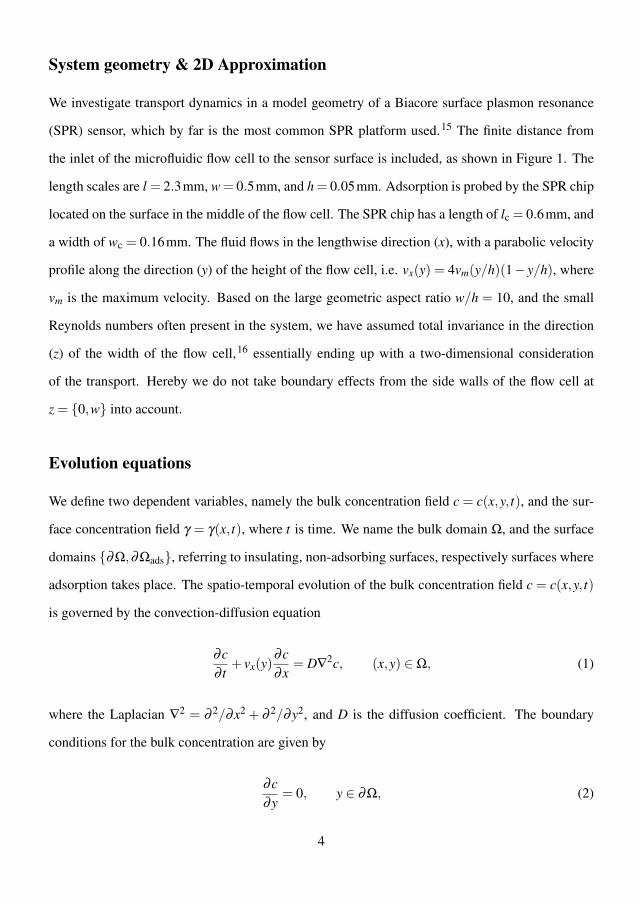
System geometry & 2D Approximation
We investigate transport dynamics in a model geometry of a Biacore surface plasmon resonance
(SPR) sensor, which by far is the most common SPR platform used.15 The finite distance from
the inlet of the microfluidic flow cell to the sensor surface is included, as shown in Figure 1. The
length scales are l = 2.3mm, w = 0.5mm, and h = 0.05mm. Adsorption is probed by the SPR chip
located on the surface in the middle of the flow cell. The SPR chip has a length of lc = 0.6mm, and
a width of wc = 0.16mm. The fluid flows in the lengthwise direction (x), with a parabolic velocity
profile along the direction (y) of the height of the flow cell, i.e. vx(y) = 4vm(y/h)(1− y/h), where
vm is the maximum velocity. Based on the large geometric aspect ratio w/h = 10, and the small
Reynolds numbers often present in the system, we have assumed total invariance in the direction
(z) of the width of the flow cell,16 essentially ending up with a two-dimensional consideration
of the transport. Hereby we do not take boundary effects from the side walls of the flow cell at
z = {0,w} into account.
Evolution equations
We define two dependent variables, namely the bulk concentration field c = c(x,y, t), and the sur-
face concentration field γ = γ(x, t), where t is time. We name the bulk domain Ω, and the surface
domains {∂Ω,∂Ωads}, referring to insulating, non-adsorbing surfaces, respectively surfaces where
adsorption takes place. The spatio-temporal evolution of the bulk concentration field c = c(x,y, t)
is governed by the convection-diffusion equation
∂c∂ t
+ vx(y)∂c∂x
= D∇2c, (x,y) ∈ Ω, (1)
where the Laplacian ∇2 = ∂ 2/∂x2 + ∂ 2/∂y2, and D is the diffusion coefficient. The boundary
conditions for the bulk concentration are given by
∂c∂y
= 0, y ∈ ∂Ω, (2)
4
92

−D∂c∂y
=−A (γ,c), y ∈ ∂Ωads. (3)
The former is simply a no-flux condition, whereas the latter is a balance between diffusive flux
perpendicular to the surface and net adsorption rate, captured in the adsorption term A (γ,c) in
Eq. (5). At the inlet of the flow cell, at x = 0, the concentration is equal to the injection con-
centration, c = c0. At the outlet of the flow cell, x = l, we assume free convection, i.e. essentially
∂c/∂x = 0. The spatio-temporal evolution of the surface concentration field γ = γ(x, t) is governed
by the adsorption-diffusion equation
∂γ∂ t
− ∂∂x
[Ds
∂γ∂x
]= A (γ,c), ∂Ωads, (4)
where Ds is the surface diffusion coefficient, which in general can be a function of both the inde-
pendent variables, x and t, as well as the dependent variables γ and c. The adsorption term A (γ,c)
represents the net rate of change of surface concentration due to adsorption and desorption. A par-
ticular functionality of A (γ,c) is determined by the kinetics of some chosen adsorption-desorption
scheme, and can in general include arbitrarily complex surface kinetics. No-flux boundary condi-
tions for γ , i.e. ∂γ/∂x = 0, are imposed at the end of the adsorbing domain, i.e. surface bound
molecules only leave the chip by desorption.
Adsorption kinetics
The adsorption kinetics is modeled by a phenomenological model, which ultimately captures ex-
perimental data and thereby provide reasonable and consistent phenomenological parameters. The
standard adsorption model that still contains the feature of a maximum surface capacity γm is the
Langmuir adsorption model. This model is essentially a first order scheme between bulk molecules
at the interface c|y=0 and free surface sites (γm−γ), with adsorption rate constant ka and desorption
rate constant kd. This first order model may be written in the form
A (γ,c) = kac|y=0(γm − γ)− kdγ. (5)
5
93
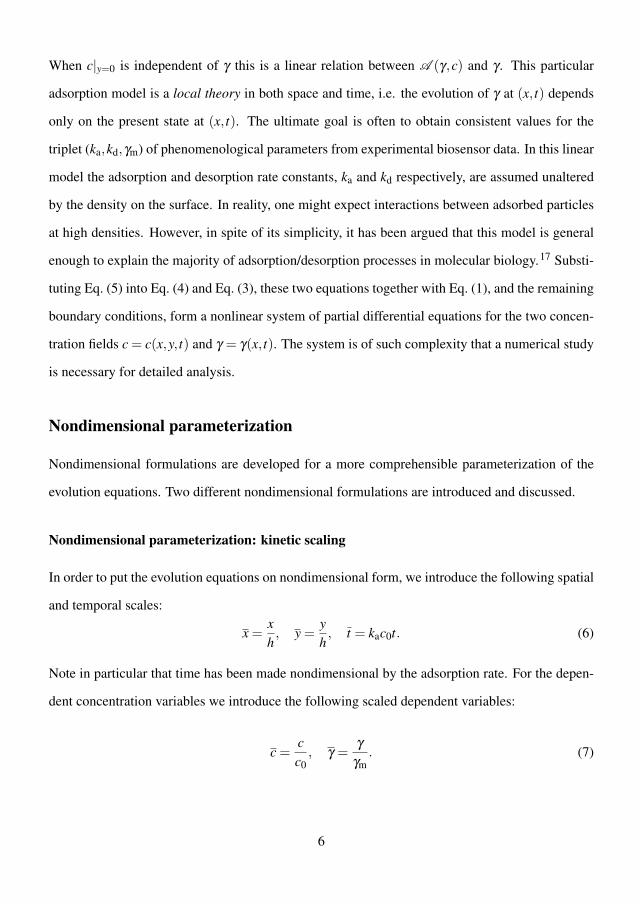
When c|y=0 is independent of γ this is a linear relation between A (γ,c) and γ . This particular
adsorption model is a local theory in both space and time, i.e. the evolution of γ at (x, t) depends
only on the present state at (x, t). The ultimate goal is often to obtain consistent values for the
triplet (ka,kd,γm) of phenomenological parameters from experimental biosensor data. In this linear
model the adsorption and desorption rate constants, ka and kd respectively, are assumed unaltered
by the density on the surface. In reality, one might expect interactions between adsorbed particles
at high densities. However, in spite of its simplicity, it has been argued that this model is general
enough to explain the majority of adsorption/desorption processes in molecular biology.17 Substi-
tuting Eq. (5) into Eq. (4) and Eq. (3), these two equations together with Eq. (1), and the remaining
boundary conditions, form a nonlinear system of partial differential equations for the two concen-
tration fields c = c(x,y, t) and γ = γ(x, t). The system is of such complexity that a numerical study
is necessary for detailed analysis.
Nondimensional parameterization
Nondimensional formulations are developed for a more comprehensible parameterization of the
evolution equations. Two different nondimensional formulations are introduced and discussed.
Nondimensional parameterization: kinetic scaling
In order to put the evolution equations on nondimensional form, we introduce the following spatial
and temporal scales:
x =xh, y =
yh, t = kac0t. (6)
Note in particular that time has been made nondimensional by the adsorption rate. For the depen-
dent concentration variables we introduce the following scaled dependent variables:
c =cc0, γ =
γγm
. (7)
6
94

In terms of these nondimensional variables, and the definitions f (y) = 4y(1− y), ∇2= ∂ 2/∂x2 +
∂ 2/∂y2 we obtain the nondimensional evolution equation for the bulk concentration field
Bic0∂c∂ t
+Pe f (y)(
∂c∂x
)= ∇2
c, Ω, (8)
with the boundary condition (Eq. (3)) given by
∂c∂y
∣∣∣∣y=0
= Bic|y=0(1− γ)−KBiγ, ∂Ωads. (9)
The nondimensional evolution equation for the surface concentration field is given by
∂γ∂ t
− ∂∂x
ds
Bic0
∂γ∂x
= c|y=0(1− γ)−Kγ, ∂Ωads. (10)
The remaining boundary conditions are trivially translated into the nondimensional form. These
nondimensional evolution equations are parameterized by the following five nondimensional groups.
Pe = vmh/D, (11)
Bi = kaγmh/D, (12)
c0 = c0h/γm, (13)
K = kd/kac0, (14)
ds = Ds/D. (15)
The Péclet number Pe measures the ratio of transport by convection to perpendicular diffusion, and
is essentially the nondimensional flow rate. The Biot number Bi measures the ratio of adsorption
rate to diffusion along the height of the flow cell, and is essentially the nondimensional adsorption
rate constant. c0 is a nondimensional inlet concentration. In the limit of no flow, c0 is the reciprocal
of the fraction of the height h needed to fill the surface up to γ = γm. This interpretation explains
the close relationship between c0 and the so called depletion depth introduced by.18 K is the kinetic
7
95

equilibrium constant. ds is the ratio of the surface and bulk diffusion coefficients, and if Ds < D,
ds ∈ {0,1} measures the hindrance of diffusion caused by the presence of the surface. Interestingly,
the magnitude of the transient term in Eq. (8) is weighed by the product c0Bi = kac0h2/D, meaning
essentially that adsorption dynamics for large inlet concentrations of molecules with a high affinity
to the surface evolves in a transient regime. This result is supported by Squires et al. 19 in their
Eq. (21).
Nondimensional parameterization: diffusion scaling
Following a similar approach as above, but with the difference of scaling time with a diffusion
time, i.e. t = Dt/h2, the nondimensional evolution equation for the bulk concentration field takes
the form
∂c∂ t
+Pe f (y)(
∂c∂x
)= ∇2
c, Ω (16)
while the boundary condition (Eq. (3)) is now given by
∂c∂y
∣∣∣∣y=0
= Bic|y=0(1− γ)−KBiγ, ∂Ωads (17)
The nondimensional evolution equation for the surface concentration field becomes
∂γ∂ t
− ∂∂x
ds∂γ∂x
= Bic0c|y=0(1− γ)−KBic0γ, ∂Ωads (18)
The correspondence between the time scales for kinetic scaling (ks) and diffusion scaling (ds) are
tks = tdskac0h2/D = Bic0tds. (19)
Kinetic scaling or diffusion scaling?
The kinetic scaling of time leads to a nondimensional formulation which is particularly advan-
tageous in the regime of kinetically limited dynamics. Generally speaking, kinetically limited
8
96

dynamics is obtained for small Bi numbers (Bi � 1) and/or large Péclet numbers (Pe � 1). Ki-
netically limited dynamics is, opposed to convection-diffusion limited dynamics, characterized by
an independence of the flow rate, i.e. Péclet number, and a scaling of the dynamics with the Biot
number. This dynamical behavior is referred to as a kinetic scaling, which is therefore also the ter-
minology used for this particular nondimensional formulation. If, on the other hand, the adsorbing
molecules have a very high affinity to the surface, Bi � 1. In this limit the dynamics is convection-
diffusion limited, which is characterized by an independence of adsorption rate, i.e. Biot number,
and a scaling of the dynamics with the Péclet number. In this limit it is advantageous to use the
diffusion scaling of time.
Disregarding the dynamical limit of the system, there are other pros and cons for applying the
two different time scales. As seen below, the quasi-steady theory adopts a minimal number of
nondimensional parameters by using kinetic scaling. Hence kinetic scaling is advantageous when
working with the quasi-steady theory. This is consistent with the fact that the quasi-steady-state
approximation is only theoretically supported for kinetically limited dynamics. This is further
elaborated on in the latter section on the quasi-steady theory. However, concerning practical use
of the theory for experimental data fitting, we remark that ka is usually a parameter one wish to
determine from an adsorption experiment, and thereby unknown a priori. Hence, kinetic scaling is
not practical for experimental data fitting - an issue avoided by using diffusion scaling. Dependent
on the experimental regime it might as well be preferable to present and fit experimental data
unscaled.
Estimates of nondimensional numbers
In this section we estimate some reasonable values for the nondimensional numbers. Concerning
typical operating conditions, flow rates are in the range Q = 1− 100 μLmin−1, which amounts
to maximum velocities of vm = 3Q/2hw = 10−3 − 10−1 ms−1. Injection concentrations typically
range from c0 = 10−1 − 102 μM. To proceed we need to consider a model binder. We take as an
9
97
example a globular protein with a diameter of 2R = 5nm, and molecular weight Mw = 30kDa =
3× 10⁴ gmol−1. A simple estimate of the maximum surface capacity γm is simply the weight of
one molecule divided by its diameter squared. Viz, γm = Mw/4NAR2 ≈ 2×10³ μgm−2, where NA
is the Avogadro number. However, in biochemical studies the surface of the chip, or the dextran
layer, is sometimes prepared with a relatively low number of binding sites, with the aim of reducing
rebinding probability and neighbor interactions among the adsorbing binders. This implies that the
above estimate for γm, which is based on a packing occurring for e.g. self-assembled monolayers,
represents an upper limit. In several applications the maximum surface capacity can be signif-
icantly lower. The diffusion coefficient can be estimated from the Stokes-Einstein relation. In
aqueous solution at room temperature, the dynamic viscosity is μ ≈ 10−3 Nsm−2, and T ≈ 300K,
hence D = kBT/6πμR ≈ 10−10 m2s−1.
Based on the above values we can estimate the regime of the nondimensional numbers. By
choosing c0 ≈ 1 μM, we obtain c0 = coh/γm ≈ 1, in the case of close packing on the surface. For
surfaces prepared with a lower number of binding sites c0 > 1. For the Péclet number we obtain
Pe = vmh/D ≈ 5×10² −5×10⁴.
The quasi-steady theory
Ideally one would like to interpret SPR data by assuming simply that the concentration near the
sensor cy=0 is identical to the injection concentration c0, that is by assuming that there is no re-
sistance to mass transfer. To account for the corrections due to some mass transfer resistance, it
has been suggested to interpret data by means of a mass transport model, saying that the overall
flux of solute J to the surface is proportional to the difference between the far field concentration
c0, usually taken as the injection concentration, and the concentration close to the surface of the
sensor c|y=0, i.e. J = kL(c0 − c|y=0). In fact, this is based on a solution to the stationary diffusion-
10
98

convection equation for the concentration field c = c(x,y) on a semi-infinite domain x,y ≥ 0.
vx∂c∂x
= D∂ 2c∂y2
, y > 0. (20)
The velocity vx = vx(y) is linearized close to the surface, i.e. vx(y) = γwy, γw being the shear
rate at the surface, and the boundary conditions for the concentration field are c(x,y)|y=0 = const,
c(x,y)|x,y→∞ = 0, and c(x,y)|x=0 = c0. The solution consists of a concentration boundary layer
close to the surface y = 0, and a flux of solute to the surface J = kL(c0 − c|y=0), where the mass
transport parameter kL is given by
kL =2D
Γ(73)
(γw
9Dl
)1/3
(21)
This mass transport parameter is often chosen as a free fitting parameter, although it may in fact be
predicted from the operating conditions. Given a flow rate Q the shear rate at the wall is
γw =6Qh2w
(22)
The coupling of this stationary convection-diffusion solution with the adsorption kinetics on the
surface is performed by loosening up the Dirichlet boundary condition c(x,y)|y=0 = const. Letting
these bulk particles c|y=0 adsorb, they are converted into surface particles γ , and a simple mass
balance on the surface dictates J = dγ/dt = A (γ,c). The critical assumption here is that the
adsorption is so slow, that the bulk concentration on the surface c|y=0 is practically constant, and
use of the steady-state flux J = kL(c0 − c|y=0), with kL given by Eq. (21), is still reasonable.
Inserting the steady-state flux into the mass balance on the surface we obtain kL(c0 − c|y=0) =
A (γ,c). In the case of linear kinetics (Eq. (5)) this becomes an algebraic equation for c|y=0, with
the solution
c|y=0 =kLc0 + kdγ
ka(γm − γ)+ kL. (23)
11
99

Substituting this into Eq. (5) gives the following nonlinear ordinary differential equation for the
evolution of the surface concentration γ = γ(t)
dγdt
=kakLc0(γm − γ)− kdkLγ
ka(γm − γ)+ kL. (24)
Using kinetic scaling, we can write Eq. (24) as
dγdt
ks
=1− (1+K)γ1+Da(1− γ)
, (25)
with the additional introduction of the important nondimensional Damköhler number
Da = kaγm/kL, (26)
which is the ratio of the adsorption rate and the rate of mass transport to the surface. The Damköh-
ler number measures the limiting effect of convection-diffusion on the adsorption process. If
Da � 1 the system is kinetically limited, and if Da � 1 the system is diffusion limited. Note
in particular when Da � 1 Eq. (25) becomes
dγdt
ks
= 1− (1+K)γ, Da � 1, (27)
which is simply the nondimensional form of Eq. (5), i.e. a purely adsorption-limited, linear, kinetic
process. Also, the initial rate of adsorption, starting from the initial condition of zero surface
concentration, γ = 0, is predicted to be
dγdt
(0)ks =1
1+Daor
dγdt
(0)ks = c0kLDa
1+Da. (28)
Using diffusion scaling the formulation of the quasi-steady theory involves the two additional
parameters, Bi and c0, viz
dγdt
ds
=Bic0(1− γ)−Kγ
Da(1− γ)−1. (29)
12
100

Correspondence between the Damköhler, Biot and Péclet Number
The kinetic scaling of the evolution equations (Eqs. (8) to (10)) clarifies the assumptions in the
quasi-steady theory. By setting Bi = 0 we essentially obtain the conditions for the solution in
Eq. (21), i.e. time dependency drops out of the bulk convection-diffusion equation, consistent with
an instantaneous build-up of the concentration boundary layer above the adsorbing surface in the
quasi-steady theory. In addition, the quasi-steady theory approximates reality by a semi-infinite
bulk domain, a linear velocity profile, and equally important, by no inlet distance to the sensor
surface.
The kinetically scaled quasi-steady theory in Eq. (25) is parameterized only by the Damköh-
ler number Da, and the equilibrium constant K. As the quasi-steady theory combines steady-
state convection-diffusion with adsorption in the Damköhler number, through the mass trans-
port coefficient kL, it is naturally possible to express the Damköhler number in terms of the Pé-
clet number and the Biot number. First, from Eq. (22), γw = 4vm/h. By defining the number
α = 2(4/9)1/3/Γ(7/3)≈ 1.2819, the mass transport coefficient kL can be expressed as
kL = α(
vmhD
)1/3 Dl1/3h2/3
Hence the Damköhler number is given by
Da =kaγm
kL= α−1(l/h)1/3 BiPe−1/3 (30)
Note that the quasi-steady theory is parameterized by the Damköhler number, and at the same
time is based on the assumption Da = 0. It is clear from Eq. (30) that the Damköhler number
increases linearly with the Biot number, and decreases with the cubic root of the Péclet number.
Practically speaking, if the binders are strongly attracted to the surface (large Biot number), it may
be impossible to reduce the Damköhler number significantly by simply increasing the flow rate,
i.e. Péclet number.
13
101
Analytical solution of the quasi-steady theory
Eq. (25) can be solved analytically in implicit form, i.e. t = t(γ) instead of the explicit form γ =
γ(t). It is determined simply by separation of variables and integration, with initially γ(t = 0) = 0:
t =Daκγ − (
κ +Da(κ −1))
ln(1−κγ)κ2
(31)
where κ ≡ 1+K. For irreversible adsorption K = 0, κ = 1, the solution condenses into
t = Daγ − ln(1− γ) (32)
This solution may not be so useful for physical insight, but has its practical advantage when per-
forming nonlinear least squares data fitting in the time domain. Data fitting in the time domain
involves a numerical solution of the ordinary differential equation (Eq. (25)) at every parameter
space iteration, which can be avoided with the implicit solution above. Another option is simply
fitting data in the phase plane.20 This method also does not involve the solution of Eq. (25), is
explicit, but as a trade off involves differentiation of data.
Numerical results and discussions
This section is concerned with a numerical investigation of the nonlinear system of partial differ-
ential equations, governing the evolution of the concentration fields. The intention is to simulate
the dynamics of real adsorption experiments in surface-based biosensors. Numerical solutions to
Eqs. (8) to (10), or similarly Eqs. (16) to (18), are collectively referred to as the simulations. We
take offset in the estimated regime for the nondimensional parameters, and to simplify matters
choose to consider the case of irreversible adsorption of binders, which are immobile on the sur-
face, hence K = ds = 0. A particular aim of the investigation is to evaluate the quality of the quasi-
steady theory by comparison with the simulations. Deviations between the simulations and the
quasi-steady theory reveal the effects of the transient dynamics in the simulations, which of course
14
102

are also present in real adsorption experiments. To mimic the case of real adsorption experiments,
being fitted by the quasi-steady theory to reveal an adsorption rate constant ka, we fit the quasi-
steady theory to the simulation with Bi as the free fitting parameter, using a least squares method.
The quasi-steady theory has no chance of fitting initial data, hence the simulation time from the ori-
gin of the phase plane to the extremum (highest adsorption rate) is cut off in the fitting procedure,
corresponding to typical practice of representing SPR data in the phase plane.20 The error of the
quasi-steady theory is then quantified by the relative difference between the fitted Bi number and
the real Bi number used for the simulation. Strictly speaking, we define the error as (Bifit−Bi)/Bi.
Being interested in the kinetics of adsorption the results are most naturally presented and analyzed
in the phase plane, spanned by the mean surface concentration Γ ≡ (1/lc)∫
sensor γ dx, and its time
derivative Γ ≡ (1/lc)∫
sensor ∂γ/∂ t dx. This representation clearly illustrates the transient regime,
and is the most straightforward approach to analyze deviations from linear adsorption kinetics due
to mass transport. The choice of parameters span both kinetically limited and convection-diffusion
limited dynamics. Results are presented using both kinetic and diffusion scaling of time, the for-
mer leading to universality for kinetically limited dynamics, and the latter leading to universality
for convection-diffusion limited dynamics. Note in particular that purely kinetically limited dy-
namics, i.e. the linear kinetics in Eq. (5), is represented by a linear curve in the phase plane. For
kinetic scaling this linear curve is the diagonal from the point (0,1) on the ordinate to the point
(1,0) on the abscissa. The universality characteristic obtained with kinetic scaling is that this curve
represents the dynamics independent of c0 and Pe for large enough Bi.
Kinetic scaling
Figure 2 contains a representative collection of phase plane curves using kinetic scaling, i.e. tks =
kac0t. Four different simulations for the combinations of concentrations c0 ∈ {1,20}, Bi ∈ {1,10},
and Pe= 500 are presented (full black line), each in a separate plot, along with the prediction of the
quasi-steady theory for identical parameters (dashed black line), as well as a fit of the quasi-steady
theory to the simulations (dashed gray line). Importantly, the quasi-steady theory scales linearly
15
103

with c0, taken into account in the kinetic scaling of time in Eq. (25). Hence the quasi-steady theory
does not explicitly include the c0 - degree of freedom, whereby essentially only two distinctive
predictions occur in Figure 2. In this way, the dashed black curves denoted (QST) are identical
in Figure 2 (a) and (b) respectively (c) and (d). Several points are immediately apparent from the
simulations. The simulation curves start at the origin of the phase plane, whereas the quasi-steady
theory has the finite initial adsorption rate given in Eq. (28). It is important to note that the kinetic
0 0.2 0.4 0.6 0.8 10
0.2
0.4
0.6
0.8
1
d/d
t (ki
netic
sca
ling)
(a) c0=1, Bi=1
SimulationQSTQST Fit
0 0.2 0.4 0.6 0.8 10
0.2
0.4
0.6
0.8
1
d/d
t (ki
netic
sca
ling)
(c) c0=1, Bi=10
SimulationQSTQST Fit
0 0.2 0.4 0.6 0.8 10
0.2
0.4
0.6
0.8
1
d/d
t (ki
netic
sca
ling)
(b) c0=20, Bi=1
SimulationQSTQST Fit
0 0.2 0.4 0.6 0.8 10
0.2
0.4
0.6
0.8
1
d/d
t (ki
netic
sca
ling)
(d) c0=20, Bi=10
SimulationQSTQST Fit
Figure 2: Phase plane dynamics using kinetic scaling. Simulation (full black line): numerical
solution of Eqs. (8) to (10). QST (dashed black line): quasi-steady theory (Eq. (25)) for corre-
sponding value of Da through Eq. (30). QST Fit (dashed gray line): fit of the quasi-steady theory
to simulation with Da as free fitting parameter. Parameters: c0 ∈ {1,20}, Bi = {1,10}, Pe = 500.
16
104

scaling of time implicitly includes a linear scaling of the adsorption rate with both Bi and c0. The
decrease in adsorption rate for both increasing Bi and increasing c0 in Figure 2, amounts to a
sublinear increase with both Bi and c0 in dimensional variables. The sublinear scaling naturally
arises from convection-diffusion limitation in the nonlinear dynamics of the system. Apart from in
the initial phase, predictions of the quasi-steady theory practically coincides with the simulations,
and thereby also the fits, for c0 = 1. Increasing the concentration to c0 = 20 leads to significant
alteration of the simulation curves. Since there are no knobs to turn for the kinetically scaled quasi-
steady theory, regarding changes in concentration c0, this leads to equally significant deviations
between the simulations and predictions of the quasi-steady theory. The observed dependency of
c0 is expected since c0 parameterizes time dependency in Eq. (8), and hence transient behavior
in the system dynamics, which is not taken into account in the quasi-steady theory. Physically
speaking, the surface simply saturates faster than a steady-state can be achieved in the bulk.
Diffusion scaling
Figure 3 contains a representative collection of phase plane curves using diffusion scaling, i.e. tds =
Dt/h2. Four different simulations for the combination of parameters c0 ∈{20}, Bi= {1,10,50,100},
and Pe = 2500 are presented, each in a separate plot, along with the prediction of the quasi-steady
theory for identical parameters, as well as a fit of the quasi-steady theory to the simulations. The
universality characteristic obtained with diffusion scaling of time is that the simulations approach
a limiting curve, representing predominantly convection-diffusion limited dynamics, for large Biot
numbers. This limiting curve in Figure 3 (d) is observed to have a very symmetric, parabolic-like,
characteristic form. Inconsistent with the simulations, quasi-steady theory predicts a linear scaling
of adsorption rate with concentration, which is explicit when using diffusion scaling as in Fig-
ure 3. This naturally leads to an increasing deviation between quasi-steady theory and simulations
for increasing Bi.
17
105
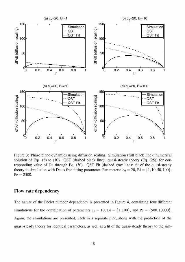
0 0.2 0.4 0.6 0.8 10
50
100
150
d/d
t (di
ffusi
on s
calin
g)(a) c
0=20, Bi=1
SimulationQSTQST Fit
0 0.2 0.4 0.6 0.8 10
50
100
150
d/d
t (di
ffusi
on s
calin
g)
(b) c0=20, Bi=10
SimulationQSTQST Fit
0 0.2 0.4 0.6 0.8 10
50
100
150
d/d
t (di
ffusi
on s
calin
g)
(c) c0=20, Bi=50
SimulationQSTQST Fit
0 0.2 0.4 0.6 0.8 10
50
100
150d
/dt (
diffu
sion
sca
ling)
(d) c0=20, Bi=100
SimulationQSTQST Fit
Figure 3: Phase plane dynamics using diffusion scaling. Simulation (full black line): numerical
solution of Eqs. (8) to (10). QST (dashed black line): quasi-steady theory (Eq. (25)) for cor-
responding value of Da through Eq. (30). QST Fit (dashed gray line): fit of the quasi-steady
theory to simulation with Da as free fitting parameter. Parameters: c0 = 20, Bi = {1,10,50,100},
Pe = 2500.
Flow rate dependency
The nature of the Péclet number dependency is presented in Figure 4, containing four different
simulations for the combination of parameters c0 = 10, Bi = {1,100}, and Pe = {500,10000}.
Again, the simulations are presented, each in a separate plot, along with the prediction of the
quasi-steady theory for identical parameters, as well as a fit of the quasi-steady theory to the sim-
18
106
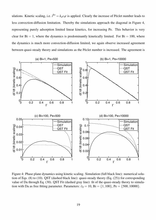
ulations. Kinetic scaling, i.e. tks = kac0t is applied. Clearly the increase of Péclet number leads to
less convection-diffusion limitation. Thereby the simulations approach the diagonal in Figure 4,
representing purely adsorption limited linear kinetics, for increasing Pe. This behavior is very
clear for Bi = 1, where the dynamics is predominantly kinetically limited. For Bi = 100, where
the dynamics is much more convection-diffusion limited, we again observe increased agreement
between quasi-steady theory and simulations as the Péclet number is increased. The agreement is
0 0.2 0.4 0.6 0.8 10
0.2
0.4
0.6
0.8
1
d/d
t (ki
netic
sca
ling)
(a) Bi=1, Pe=500
SimulationQSTQST Fit
0 0.2 0.4 0.6 0.8 10
0.01
0.02
0.03
0.04
0.05
d/d
t (ki
netic
sca
ling)
(c) Bi=100, Pe=500
SimulationQSTQST Fit
0 0.2 0.4 0.6 0.8 10
0.2
0.4
0.6
0.8
1
d/d
t (ki
netic
sca
ling)
(b) Bi=1, Pe=10000
SimulationQSTQST Fit
0 0.2 0.4 0.6 0.8 10
0.02
0.04
0.06
0.08
0.1
0.12
d/d
t (ki
netic
sca
ling)
(d) Bi=100, Pe=10000
SimulationQSTQST Fit
Figure 4: Phase plane dynamics using kinetic scaling. Simulation (full black line): numerical solu-
tion of Eqs. (8) to (10). QST (dashed black line): quasi-steady theory (Eq. (25)) for corresponding
value of Da through Eq. (30). QST Fit (dashed gray line): fit of the quasi-steady theory to simula-
tion with Da as free fitting parameter. Parameters: c0 = 10, Bi = {1,100}, Pe = {500,10000}.
19
107

however not as good as for Bi = 1. Note that the ordinate axis are different in Figure 4 (c) and (d)
where Bi = 100. The specific case in Figure 4 (c), where c0 = 10, Bi = 100, Pe = 500, is clearly
in a regime where the quasi-steady theory has little value, and little ability to fit data well. The
approach to adsorption limited dynamics is consistent with a decrease in the Damköhler number
as Da ∼ Pe−1/3 from Eq. (30). Figure 4 also serves to show that, due to this slow cubic root de-
pendency, experimental practicalities often precludes to cope with convection-diffusion limitation
by simply increasing the flow rate for systems with a high Biot number.
In summary, Figures 2 to 4 stress some nonlinearities present in the real system dynamics,
which are not well captured in the approximate quasi-steady theory.
Error of the quasi-steady theory
The numerical investigation concludes with a quantification of the error of the quasi-steady theory,
measured as the relative difference between the Biot number used to fit the quasi-steady theory
to simulations, and the Biot number used for the simulation itself. The nondimensional parameter
space is spanned by Bi∈ {1, . . . ,100}, Pe∈ {500, . . . ,10000}, for c0 = {1,10,20}. Figure 5 (a)-(c)
present the relative error (Bifit −Bi)/Bi, by contour lines in the nondimensional parameter space
(Pe,Bi), for c0 = {1,10,20} respectively. Every contour is labelled with the matching error. Equal
for all values of c0 is that the error is largest for slow flows of strong binders, i.e. small Pe and large
Bi numbers. For c0 = 1 only relatively minor errors, up to around 0.2 (20%), are observed in the
spanned parameter space. However, the quantitative increase of the error with c0 is significant. For
c0 = 20 the errors increase to above 2.5 (250%), which amounts to a factor of 3-4, in the spanned
parameter space. Importantly, the quasi-steady theory consequently overestimates the Biot number,
and thereby the adsorption rate constant, as long as the error is over a few percent. (Below errors
of a few percent the fit and the prediction are so close that this is not always the case.) Hence,
the parameter planes showed in Figure 5 provide a tool to quantitatively correct experimentally
obtained adsorption rate constants, which are derived by fitting data with the quasi-steady theory.
20
108
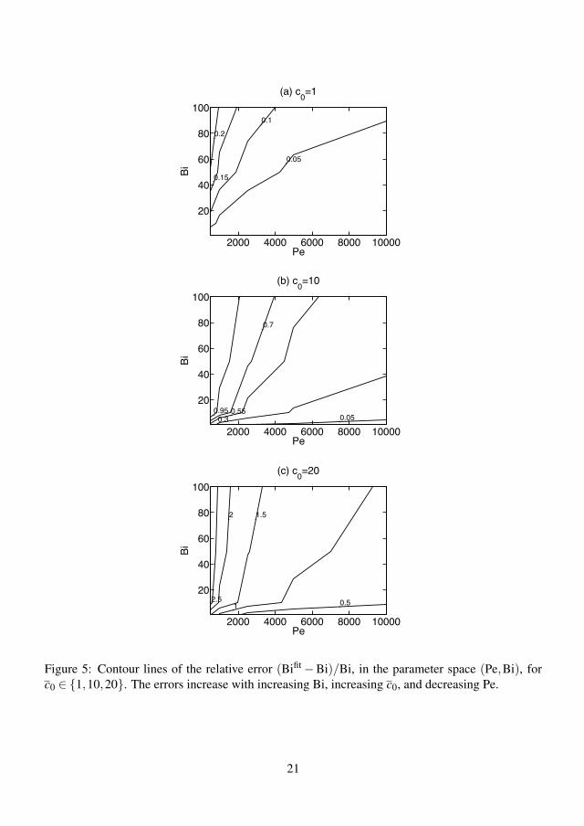
0.05
0.1
0.15
0.2
Pe
Bi
(a) c0=1
2000 4000 6000 8000 10000
20
40
60
80
100
0.050.30.55
0.7
0.95
Pe
Bi
(b) c0=10
2000 4000 6000 8000 10000
20
40
60
80
100
0.51
1.52
2.5
Pe
Bi
(c) c0=20
2000 4000 6000 8000 10000
20
40
60
80
100
Figure 5: Contour lines of the relative error (Bifit −Bi)/Bi, in the parameter space (Pe,Bi), for
c0 ∈ {1,10,20}. The errors increase with increasing Bi, increasing c0, and decreasing Pe.
21
109

Conclusion
This paper presented theoretical and computational investigations of convection, diffusion, and
adsorption dynamics in microfluidic surface-based biosensors. The nondimensional Damköhler
number Da = kaγm/kL, inherent in the quasi-steady theory, was expressed in terms of the Biot
number Bi = kaγmh/D, the Péclet number Pe = vmh/D, and the model geometry. In addition, an
analytical solution to the quasi-steady theory was derived. The results provided the regimes of both
reliable and unreliable use of the quasi-steady theory for experimental data analysis, by quantifying
the error of the quasi-steady theory in the space of parameters. This can be used as a tool to
correct adsorption rate constants obtained by fitting the quasi-steady theory to experimental data.
We deduced a critical importance of the inlet concentration, and the maximum surface capacity,
combined in the nondimensional inlet concentration.
References
(1) Stenberg, E.; Persson, B.; Roos, H.; Urbaniczky, C. Journal of Colloid and Interface Science
1991, 143, 513 – 526.
(2) Homola, J.; Yee, S.; Gauglitz, G. SENSORS AND ACTUATORS B-CHEMICAL 1999, 54,
3–15.
(3) Homola, J. Chem Rev 2008, 108, 462–93.
(4) Schuck, P.; Minton, A. ANALYTICAL BIOCHEMISTRY 1996, 240, 262–272.
(5) Myszka, D. G.; He, X.; Dembo, M.; Morton, T. A.; Goldstein, B. Biophys J 1998 Aug, 75,
583–594.
(6) Schuck, P. Biophys J 1996, 70, 1230–49.
(7) Schuck, P.; Minton, A. P. Anal Biochem 1996, 240, 262–72.
(8) Mason, T.; Pineda, A. R.; Wofsy, C.; Goldstein, B. Math Biosci 1999, 159, 123–44.
22
110

(9) Noinville, S.; Vidic, J.; Déjardin, P. Colloids Surf B Biointerfaces 2010, 76, 112–6.
(10) Goldstein, B.; Coombs, D.; He, X.; Pineda, A. R.; Wofsy, C. J Mol Recognit 1999 Sep-Oct,
12, 293–299.
(11) Rich, R. L.; Myszka, D. G. J Mol Recognit 2011, 24, 892–914.
(12) Rich, R. L.; Myszka, D. G. J Mol Recognit 2010, 23, 1–64.
(13) Rich, R. L.; Myszka, D. G. J Mol Recognit 2008, 21, 355–400.
(14) Rich, R. L.; Myszka, D. G. J Mol Recognit 2007, 20, 300–66.
(15) Besenicar, M.; Macek, P.; Lakey, J. H.; Anderluh, G. Chem Phys Lipids 2006, 141, 169–78.
(16) Brody, J. P.; Yager, P.; Goldstein, R. E.; Austin, R. H. Biophys J 1996, 71, 3430–41.
(17) Gervais, T.; Jensen, K. F. Chemical Engineering Science 2006, 61, 1102 – 1121.
(18) Alvarez, N. J.; Walker, L. M.; Anna, S. L. Phys. Rev. E 2010, 82, 011604.
(19) Squires, T. M.; Messinger, R. J.; Manalis, S. R. Nat Biotechnol 2008, 26, 417–26.
(20) Goren, M.; Galley, N.; Lennox, R. B. Langmuir 2006 Jan 31, 22, 1048–1054.
23
111

112

[P2]
113

114
Rheol Acta (2010) 49:555–562DOI 10.1007/s00397-010-0434-0
ORIGINAL CONTRIBUTION
Constitutive equations for the Doi–Edwards modelwithout independent alignment
Ole Hassager · Rasmus Hansen
Received: 25 October 2009 / Accepted: 12 January 2010 / Published online: 6 March 2010© Springer-Verlag 2010
Abstract We present two representations of the Doi–Edwards model without Independent Alignment ex-plicitly expressed in terms of the Finger strain tensor,its inverse and its invariants. The two representationsprovide explicit expressions for the stress prior to andafter Rouse relaxation of chain stretch, respectively.The maximum deviations from the exact representa-tions in simple shear, biaxial extension and uniaxialextension are of order 2%. Based on these two repre-sentations, we propose a framework for Doi–Edwardsmodels including chain stretch in the memory integralform.
Keywords Constitutive equation · Nonlinearviscoelasticity ·Orientation tensor · Strain energydensity · Second normal stress difference · Tube model
Introduction
Representing a landmark in our understanding of thedynamics of entangled polymeric systems, the Doi–Edwards model (DE) model (Doi and Edwards 1986)is based on a set of remarkably simple model assump-tions (Doi 1995). The basic DEmodel for the nonlinear
Paper presented at the 5th Annual European RheologyConference, April 15–17, 2009, Cardiff, United Kingdom.
O. Hassager (B) · R. HansenDanish Polymer Center, Department of Chemical andBiochemical Engineering, Technical University of Denmark,2800 Kgs. Lyngby, Denmarke-mail: [email protected]
viscoelastic properties contains two key assumptionsabout how the central axis of the tube deforms undera macroscopic deformation. It is assumed that the tubeaxis deforms affinely with the deformation, and thatafter a time τR, the tube length returns to its equilibriumvalue.The basic DE model is found in two versions, one
with the so-called Independent Alignment (IA) ap-proximation and one without this approximation (Doiand Edwards 1978). Both models require the calcu-lation of an integral over the unit sphere for eachstress evaluation. Methods for fast stress evaluationare therefore interesting (Mead et al. 1995). Especiallyconvenient expressions have been presented by Currie(1982a, b), who formulated BKZmemory integral mod-els (Bird et al. 1987) intended to approximate the con-stitutive equation for the DE model both with (Currie1982a) and without (Currie 1982b) IA invoked.The Currie equation with IA has been used and
tested extensively in modeling and simulation of poly-mer flow (Marin and Rasmussen 2009; Wapperomand Keunings 2001; Blackwell et al. 2000; Olley 2005;Mead 2007; Peters et al. 2000; Olley and Wagner 2006;Wagner 1990). The Currie equation without IA hasreceived much less attention, nor does the accuracyof approximation seem to have been systematicallytested, possibly because Currie states that it “differslittle in its predictions” from the approximation to theIA version. This latter statement, however does seemin contrast to the observations that the nonlinear rhe-ological properties of the DE model with and withoutIA differ markedly in specific flow situations. Thus, theDE model with IA predicts a negative Weissenbergeffect (Hassager 1985) while the version without IApredicts a positive Weissenberg effect as pointed out by
115

556 Rheol Acta (2010) 49:555–562
Marrucci and Grizzuti (1986) who performed a carefulcomparison of the two versions at second order.The purpose of this work is to derive constitutive
equations for the DE model without IA both prior toand after Rouse relaxation (Doi and Edwards 1986)and to evaluate the accuracy of the approximations insimple shear, biaxial extension and uniaxial extension.To fix ideas and notation we briefly recapitulate thederivation of the relevant equations starting from theexpression for the free energy of deformation of anentanglement network (Doi 1995; Hansen et al. 2008)
A = 3
2nc Z kT〈|E · u|〉2
u (1)
Here nc is the number density of chains, Z the numberof entanglements per chain, k Boltzmanns constant,and T the absolute temperature. Furthermore, E is thedeformation gradient (Bird et al. 1987) from the stress-free state to the current state, u is a unit vector, and〈· · · 〉u denotes an average over the orientation of the 3-dimensional unit vector u, i.e., an isotropic distribution.From this expression, it is straightforward to derive(e.g. Hansen et al. 2008) the corresponding expressionfor the macroscopic stress tensor,
σ netij = G0
15
4〈|E · u|〉u
⟨ Eimum E jnun
|E · u|⟩u
(2)
where the elastic modulusG0 = (4/5)nc Z kT. The com-bination of factors after the modulus is sometimesreferred to as a strain tensor, since it reduces to theinfinitesimal strain tensor in the small strain limit. Thedecoration “net” signifies that the expression relatesto an entanglement network without relaxation of theoverall chain length.Consider now an entangled polymer melt subject
to a single fast deformation given by the deformationgradient E. For time t > τR when the tube has relaxedto its equilibrium value, the stress is reduced by thesquare of the initial chain stretch to obtain,
σij = GN0
15
4〈|E · u|〉−1
u
⟨Eimum E jnun
|E · u|⟩
u(3)
where the plateau modules GN0 = (4/5)nc Z kT is un-
changed since the average stretch is unity in the smallstrain limit. To simplify further, Doi and Edwardsintroduced the Independent Alignment Assumption,which effectively replaces the ratio of averages with theaverage of the ratio. Such a replacement is problematicas Doi and Edwards were well aware (Doi and Edwards1986). Thus for small deformations, the ratio of the
averages and the average of the ratio are expanded inthe infinitesimal strain tensor εij respectively as follows:
〈|E · u|〉−1u
⟨Eimum E jnun
|E · u|⟩
u= δij + 4
15εij + O
(ε2
ij
)(4)
⟨Eimum E jnun
|E · u||E · u|⟩
u= δij + 1
5εij + O
(ε2
ij
)(5)
In other words, the only term correctly reproduced inthe IA approximation is the unit tensor. But the unittensor has no rheological significance. The linear termin εij is under-predicted by a factor of 3/4. This factoris not a problem in practical applications, since one cansimply scale the modulus accordingly (Mead 2007). Butthe difference between the O(ε2
ij) terms in Eqs. 4 and 5is at the heart of the difference between negative andpositive Weissenberg effects (Marrucci and Grizzuti1986).From the above it appears that we need to approxi-
mate 〈|E · u|〉2u in terms of the invariants of the Finger
and Cauchy strain tensors of nonlinear elasticity. Fol-lowing Currie, we consider in turn an exact expression,an asymptotic form, and the small strain expansion.The final approximation is arrived at by matching theasymptotic form with the small strain expansion.
Evaluation of potential function
For uniaxial and biaxial deformation one may utilizethe axial symmetry to obtain the simple analyticalexpressions for the desired integral (Urakawa et al.1995). We list the expressions for future reference. Foruniaxial extension λ1 = λ and λ2 = λ3 = λ−1/2 the exactexpression is
〈|E · u|〉 = 1
2λ + 1
4
λ−1
√λ2 − λ−1
logλ + √
λ2 − λ−1
λ − √λ2 − λ−1
(6)
For biaxial extension λ1 = λ2 = λ and λ3 = λ−2 the ex-act expression is
〈|E · u|〉 = 1
2
(λ−2 + λ√
1 − λ−6sin−1
√1 − λ−6
)(7)
For general deformations we need to compute
〈|E · u|〉 =⟨√
Bijuiu j
⟩(8)
where Bij = Emi Emj is not the same as the Fingerstrain tensor Bij = Eim E jm but the two matrices havethe same eigenvalues λ2
i for i = 1, 2, 3. Without loss ofgenerality we can order the eigenvalues λ2
1 ≥ λ22 ≥ λ2
3.
116
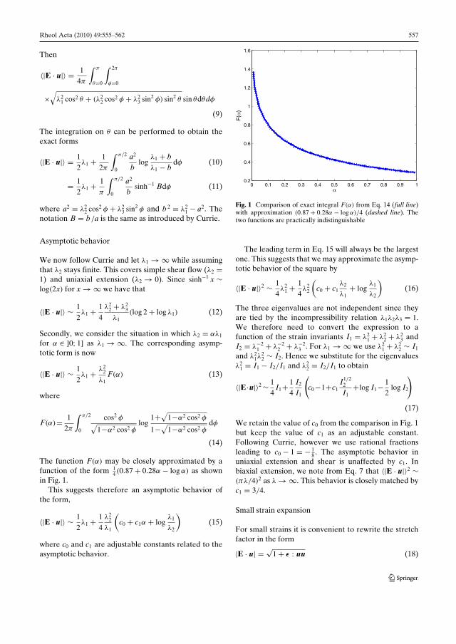
Rheol Acta (2010) 49:555–562 557
Then
〈|E · u|〉 = 1
4π
∫ π
θ=0
∫ 2π
φ=0
×√
λ21 cos2 θ + (λ2
2 cos2 φ + λ23 sin2 φ) sin2 θ sin θdθdφ
(9)
The integration on θ can be performed to obtain theexact forms
〈|E · u|〉 = 1
2λ1 + 1
2π
∫ π/2
0
a2
blog
λ1 + bλ1 − b
dφ (10)
= 1
2λ1 + 1
π
∫ π/2
0
a2
bsinh−1 Bdφ (11)
where a2 = λ22 cos2 φ + λ2
3 sin2 φ and b 2 = λ21 − a2. The
notation B = b/a is the same as introduced by Currie.
Asymptotic behavior
We now follow Currie and let λ1 → ∞ while assumingthat λ2 stays finite. This covers simple shear flow (λ2 =1) and uniaxial extension (λ2 → 0). Since sinh−1 x ∼log(2x) for x → ∞ we have that
〈|E · u|〉 ∼ 1
2λ1 + 1
4
λ22 + λ2
3
λ1(log 2 + log λ1) (12)
Secondly, we consider the situation in which λ2 = αλ1
for α ∈ ]0; 1] as λ1 → ∞. The corresponding asymp-totic form is now
〈|E · u|〉 ∼ 1
2λ1 + λ2
2
λ1F(α) (13)
where
F(α)= 1
2π
∫ π/2
0
cos2 φ√1−α2 cos2 φ
log1+√
1−α2 cos2 φ
1−√1−α2 cos2 φ
dφ
(14)
The function F(α) may be closely approximated by afunction of the form 1
4 (0.87 + 0.28α − log α) as shownin Fig. 1.This suggests therefore an asymptotic behavior of
the form,
〈|E · u|〉 ∼ 1
2λ1 + 1
4
λ22
λ1
(c0 + c1α + log
λ1
λ2
)(15)
where c0 and c1 are adjustable constants related to theasymptotic behavior.
0 0.1 0.2 0.3 0.4 0.5 0.6 0.7 0.8 0.9 10.2
0.4
0.6
0.8
1
1.2
1.4
1.6
α
F(α
)
Fig. 1 Comparison of exact integral F(α) from Eq. 14 (full line)with approximation (0.87 + 0.28α − log α)/4 (dashed line). Thetwo functions are practically indistinguishable
The leading term in Eq. 15 will always be the largestone. This suggests that we may approximate the asymp-totic behavior of the square by
〈|E · u|〉2 ∼ 1
4λ2
1 + 1
4λ2
2
(c0 + c1
λ2
λ1+ log
λ1
λ2
)(16)
The three eigenvalues are not independent since theyare tied by the incompressibility relation λ1λ2λ3 = 1.We therefore need to convert the expression to afunction of the strain invariants I1 = λ2
1 + λ22 + λ2
3 andI2 = λ−2
1 + λ−22 + λ−2
3 . For λ1 → ∞ we use λ21 + λ2
2 ∼ I1
and λ21λ
22 ∼ I2. Hence we substitute for the eigenvalues
λ21 = I1 − I2/I1 and λ2
2 = I2/I1 to obtain
〈|E·u|〉2 ∼ 1
4I1+ 1
4
I2
I1
(c0−1+c1
I1/22
I1+log I1− 1
2log I2
)
(17)
We retain the value of c0 from the comparison in Fig. 1but keep the value of c1 as an adjustable constant.Following Currie, however we use rational fractionsleading to c0 − 1 = − 1
8 . The asymptotic behavior inuniaxial extension and shear is unaffected by c1. Inbiaxial extension, we note from Eq. 7 that 〈|E · u|〉2 ∼(πλ/4)2 as λ → ∞. This behavior is closely matched byc1 = 3/4.
Small strain expansion
For small strains it is convenient to rewrite the stretchfactor in the form
|E · u| = √1 + ε : uu (18)
117

558 Rheol Acta (2010) 49:555–562
where ε = diag(λ21 − 1, λ2
2 − 1, λ23 − 1) = diag(ε1, ε2, ε3).
The εi are not independent due to the incompressibilitycondition. But we may choose ε1 and ε2 as free parame-ters. Then to third order,
ε3 = −ε1 − ε2 + ε21 + ε2
2 + ε1ε2 − ε31
−ε21ε2 − ε1ε
22 − ε3
2 + O(ε4) (19)
where O(ε4) indicates terms εi1ε
j2 with i + j ≥ 4. Like-
wise the two strain invariants need to be expanded
I1 − 3 = ε21 + ε2
2 + ε1ε2 − ε31 − ε2
1ε2 − ε1ε22 − ε3
2 + O(ε4)
(20)
I2 − 3 = ε21 + ε2
2 + ε1ε2 − ε31 − ε3
2 + O(ε4) (21)
By expansion of Eq. 18 for small strains one obtains
|E · u| = 1 + 1
2εijuiu j − 1
8εijεkluiu jukul
+ 3
48εijεklεmnuiu jukulumun + · · · (22)
It is now straightforward but somewhat tedious to ob-tain the expansion for 〈|E · u|〉 to third order in the εi
by utilizing the expression for averages of products ofunit vectors over the unit sphere. Explicit expression tosixth order in the ui as needed here may be found inBird et al. (1977). By matching the resulting expressionwith Eqs. 20 and 21 one obtains to first order in thestrain invariants,
〈|E · u|〉 = 1 + 2
105(6(I1 − 3) + (I2 − 3)) + · · · (23)
Hence the potential becomes
〈|E · u|〉2 = 1 + 4
105(6(I1 − 3) + (I2 − 3)) + · · · (24)
Matching expression
We now wish to construct a function U(I1, I2) thatmatches the asymptotic behavior of 〈|E · u|〉2 in Eq. 17with the small strain behavior in Eq. 24. In particularwe propose
U(I1, I2) = 1
4I1+ 1
4
I2
I1
(−1
8+ 3
4
I1/22
I1+log I1− 1
2log I2
)
+a1
I1+ a2
I2+ a3 (25)
for some constants ai (i = 1, 2, 3) that are determinedby the requirements
U(3, 3) = 1 (26)
∂U∂ I1
(3, 3) = 8
35(27)
∂U∂ I2
(3, 3) = 4
105(28)
The following results are obtained,
a1 = +1161
1120− 3
√3
8− 3
8log 3
.= −0.0249 (29)
a2 = − 909
1120+ 9
√3
32+ 3
8log 3
.= +0.0875 (30)
a3 = + 33
160− 1
32
√3 − 1
8log 3
.= +0.0148 (31)
The small numerical values of the constants ai indicatesthat the asymptotic form is already a reasonable goodapproximation to the potential. We may check thefunction U(I1, I2) along the two types of deformationthat span the available invariant space, namely uniaxial(Fig. 2) and biaxial (Fig. 3) extension.It appears that the potential in Eq. 25 approximates
the exact potential to better than 2.5% in uniaxial andbiaxial deformations. Since these two types of defor-mation bound the available space for the invariants I1
and I2 we use it as approximation in the entire invariantspace.
1 1.5 2 2.5 3 3.5 4 4.5 51
2
3
4
5
6
7ExactApproximate
Fig. 2 Plot of approximate potential U from Eq. 25 and exactpotential Eq. 6 in uniaxial deformation as function of λ. Thetwo curves practically overlap. The maximum relative deviation(2.3%) occurs at intermediate λ values
118
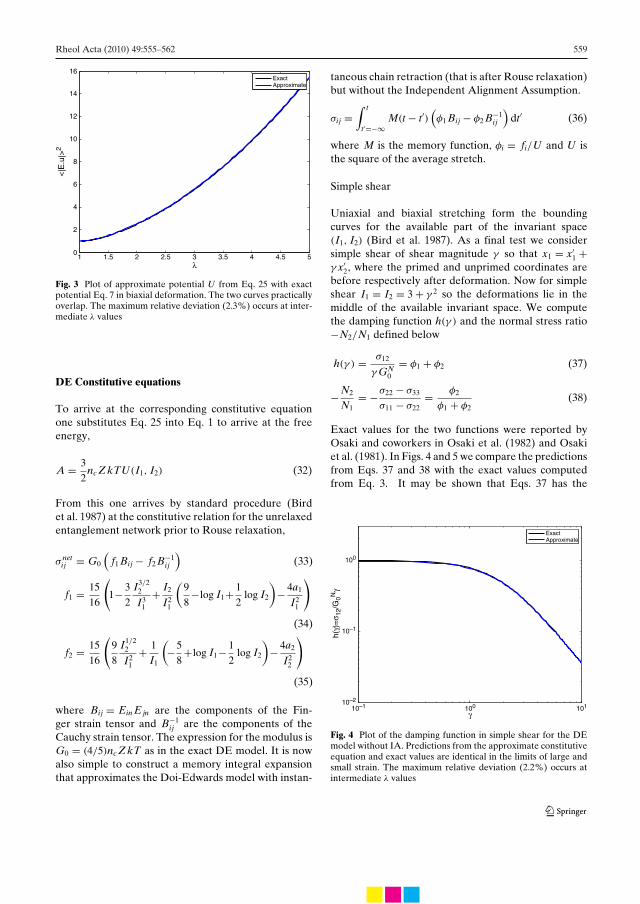
Rheol Acta (2010) 49:555–562 559
1 1.5 2 2.5 3 3.5 4 4.5 50
2
4
6
8
10
12
14
16ExactApproximate
Fig. 3 Plot of approximate potential U from Eq. 25 with exactpotential Eq. 7 in biaxial deformation. The two curves practicallyoverlap. The maximum relative deviation (2.3%) occurs at inter-mediate λ values
DE Constitutive equations
To arrive at the corresponding constitutive equationone substitutes Eq. 25 into Eq. 1 to arrive at the freeenergy,
A = 3
2nc Z kTU(I1, I2) (32)
From this one arrives by standard procedure (Birdet al. 1987) at the constitutive relation for the unrelaxedentanglement network prior to Rouse relaxation,
σ netij = G0
(f1 Bij − f2 B−1
ij
)(33)
f1 = 15
16
(1− 3
2
I3/22
I31
+ I2
I21
(9
8−log I1+ 1
2log I2
)− 4a1
I21
)
(34)
f2 = 15
16
(9
8
I1/22
I21
+ 1
I1
(−5
8+log I1− 1
2log I2
)− 4a2
I22
)
(35)
where Bij = Ein E jn are the components of the Fin-ger strain tensor and B−1
ij are the components of theCauchy strain tensor. The expression for the modulus isG0 = (4/5)nc Z kT as in the exact DE model. It is nowalso simple to construct a memory integral expansionthat approximates the Doi-Edwards model with instan-
taneous chain retraction (that is after Rouse relaxation)but without the Independent Alignment Assumption.
σij =∫ t
t′=−∞M(t − t′)
(φ1 Bij − φ2 B−1
ij
)dt′ (36)
where M is the memory function, φi = fi/U and U isthe square of the average stretch.
Simple shear
Uniaxial and biaxial stretching form the boundingcurves for the available part of the invariant space(I1, I2) (Bird et al. 1987). As a final test we considersimple shear of shear magnitude γ so that x1 = x′
1 +γ x′
2, where the primed and unprimed coordinates arebefore respectively after deformation. Now for simpleshear I1 = I2 = 3 + γ 2 so the deformations lie in themiddle of the available invariant space. We computethe damping function h(γ ) and the normal stress ratio−N2/N1 defined below
h(γ ) = σ12
γ GN0
= φ1 + φ2 (37)
− N2
N1= −σ22 − σ33
σ11 − σ22= φ2
φ1 + φ2(38)
Exact values for the two functions were reported byOsaki and coworkers in Osaki et al. (1982) and Osakiet al. (1981). In Figs. 4 and 5 we compare the predictionsfrom Eqs. 37 and 38 with the exact values computedfrom Eq. 3. It may be shown that Eqs. 37 has the
10–1 100 10110–2
10–1
100
ExactApproximate
Fig. 4 Plot of the damping function in simple shear for the DEmodel without IA. Predictions from the approximate constitutiveequation and exact values are identical in the limits of large andsmall strain. The maximum relative deviation (2.2%) occurs atintermediate λ values
119

560 Rheol Acta (2010) 49:555–562
10–1 100 10110–2
10–1
ExactApproximate
Fig. 5 Plot of the normal stress ratio in simple shear for the DEmodel without IA. Predictions from the approximate constitutiveequation and exact values are identical in the limits of large andsmall strain. The maximum relative deviation (1.8%) occurs atintermediate λ values
behavior h(γ ) ∼ (15/4)γ −2 as γ → ∞ which is exactlythe same asymptotic behavior as for the exact equationin 3. For comparison, the IA version has the asymptoticbehavior h(γ ) ∼ 5γ −2 as γ → ∞ which departs fromthe correct behavior by 33%. Also the asymptotic formof the normal stress ratio from Eq. 38 is −N2/N1 ∼γ −2 log γ which is identical to the asymptotic behaviorof the exact expression (as shown in the Appendix). Bycontrast the IA approximation changes the asymptoticbehavior to −N2/N1 ∼ γ −1. Thus the IA approxima-tion results in marked changes in the normal stressratio, not just in the low shear limit, but more drasticallyin the asymptotic behavior.In closing we note that Currie approximation for
the DE model without independent alignment (Currie1982b) approximates the damping function and thesmall shear behavior of −N2/N1 closely but fails to ap-proximate the asymptotic behavior of the normal stressratio. The Currie approximation yields −N2/N1 ∼(2
√3γ )−1 for γ → ∞, which apart from the numerical
factor is the same as the behavior for the IA version,but not the correct behavior.
Constitutive equations with stretch relaxation
The DE melt model in form Eq. 36 contains the as-sumption of instantaneous relaxation of the chains totheir equilibrium length. However it was recognizedearly that chain stretching in uncrosslinked entangledpolymer systems will occur at deformation rates fasterthan the inverse Rouse time (Maruucci and Grizzutti1988; Pearson et al. 1989). The concept of chain stretch-
ing is now standard in reptation-based models (Fanget al. 2000;Mead et al. 1998; Schieber et al. 2003). Giventhe stretch function U(I1, I2) it is straightforward toformulate models with Rouse dynamics for the chainstretch. For example assuming that stretch relaxation isdominated by a single Rouse relaxation time, a possibledescription (Lyhne et al. 2009) would be:
λ2(t, t′) =[1 + (
√U(t, t′) − 1) exp(−(t − t′)/τR)
]2(39)
where the stretch relaxation time τR is the Rouse time.The corresponding constitutive equation is then,
σij =∫ t
t′=−∞λ2(t, t′)M(t − t′)
(φ1 Bij − φ2 B−1
ij
)dt′. (40)
Conclusions
The key to the constitutive equations is the develop-ment of an accurate representation of the unrelaxedentanglement network in terms of the invariants of theFinger strain tensor. Based on this representation it hasbeen possible to formulate constitutive equations forthe unrelaxed network and for the completely relaxednetwork both without the independent alignment ap-proximation. The representations have the exact be-havior for small strain and show the correct asymp-totic behavior in simple shear, biaxial and uniaxialdeformations. In the intermediate range, the maximumdeviations from the exact behavior in the deformationsinvestigated is of order 2%. In closing, a model isproposed for a network with partial relaxation, corre-sponding to a DE model with chain stretch. It is formu-lated in a form with a single stretch relaxation time, butmay easily be generalized to multiple relaxation times.
Acknowledgements The authors would like to thank StigWedel and Jose Marin for critical and constructive comments.Rasmus Hansen is supported by the Danish Agency for Science,Technology and Production and by Novozymes A/S.
Appendix on asymptotic normal stress ratio in shear
Given a shear deformation of magnitude γ , the lengthof the deformed unit vector may be written in the form
|E · u| = (1 + sin2 θ f (φ)
)1/2(41)
where f (φ) is given by
f (φ) = 1
2
(1 + γ 2
)(1 − cos 2φ) + γ sin 2φ (42)
120

Rheol Acta (2010) 49:555–562 561
It follows that f (φ) has a minimum at
φm = −1
2tan−1 2γ
1 + γ 2∼ −γ −1 for γ → ∞ (43)
It may be shown that f (φ) has the Taylor expansion
f (φ) = (−1 + 2γ −2) + (φ + γ −1)2
γ 2 + · · · (44)
around φ = −γ −1. It follows that in this region we mayapproximate
|E · u| = γ sin θ(a2 + x2
)1/2(45)
where
a2 = γ −2 (cot2 θ + 2γ −2)
and x = φ + γ −1.The negative of the second normal stress is com-
puted from
(σzz − σyy)/G0 = I = 1
4π
∫ π
θ=0
∫ 2π
φ=0
×(cos2 θ−sin2 θ sin2 φ
)sin θdθdφ
|E · u| (46)
The periodicity of the harmonic functions may be uti-lized to show that
I = 1
π
∫ π/2
θ=0
∫ π
φ=0
(cos2 θ − sin2 θ sin2 φ
)sin θdθdφ
|E · u| (47)
= 1
π
∫ π/2
θ=0
∫ π−γ −1
φ=−γ −1
(cos2 θ − sin2 θ sin2 φ
)sin θdθdφ
|E · u|(48)
≈ 2
πγ
∫ π/2
θ=0
∫ A
x=0
(cos2 θ − sin2 θ sin2
(x − γ −1
))dθdx(
a2 + x2)1/2
(49)
In going from Eqs. 48 to 49 we have used that the majorcontribution to the integral will occur near x = 0 andthat the maximum becomes symmetric around x = 0.We therefore integrate up to some limit A ∈ [0; π/2],the exact value of which does not influence the asymp-totic behavior. Moreover sin2(x − γ −1))will be of orderγ −2 near x = 0 so the term with sin2 θ in the numeratorof Eq. 49 may be neglected in the limiting process. Wenow use that∫ A
0
dx(a2 + x2
)1/2 = log |x +√
a2 + x2|A0
Examination of the leading terms shows that eventually
(σzz − σyy)/G0 ∼ 1
2γ −1(C + log γ ) (50)
where the constant C is included to indicate the orderof the terms neglected.The first normal stress difference is much easier to
compute with the result
(σxx − σyy)/G0 ∼ 1
2γ for γ → ∞ (51)
The combined result is
− N2
N1∼ γ −2 (log γ + C) for γ → ∞ (52)
Numerical computations show that C ≈ −0.6.
References
Bird RB, Hassager O, Armstrong RC, Curtiss CF (1977) Dynam-ics of polymeric liquids: kinetic theory, vol 2, 1st edn. Wiley,New York
Bird RB, Armstrong RC, Hassager O (1987) Dynamics of poly-meric liquids: fluid mechanics, vol 1. Wiley, New York
Blackwell RJ, McLeish TCB, Harlen OG (2000) Molecular drag-strain coupling in branched polymer melts. J Rheol 44:121–136
Currie PK (1982a) Constitutive equations for polymer melts pre-dicted by the Doi-Edwards and Curtiss-Bird kinetic theorymodels. J Non-Newtonian Fluid Mech 11:53–68
Currie PK (1982b) Relationship between extensional and shearproperties of polymer melts as predicted by the Doi–Edwards model. Polymer Preprints 23:6–7
DoiM (1995) Introduction to polymer physics. OxfordUniversityPress, New York
Doi M, Edwards SF (1978) J Chem Soc Faraday Trans 2:74 1802Doi M, Edwards SF (1986) The theory of polymer dynamics.
Oxford University Press, New YorkFang J, Kröger M, Öttinger HC (2000) J Rheol 44:1293–1317Hansen R, Skov AL, Hassager O (2008) Constitutive equation
for polymer networks with phonon fluctuations. Phys Rev E77:011802
Hassager O (1985) J Rheol 29:361Lyhne A, Rasmussen HK, Hassager O (2009) Phys Rev Lett
102:138301Marin JMR, Rasmussen HK (2009) Lagrangian finite-element
method for the simulation of K-BKZ fluids with third orderaccuracy. J Non-Newtonian Fluid Mech 156:177–188
Marrucci G, Grizzuti N (1986) The Doi–Edwards model inslow flows. Predictions of the Weissenberg effect. J Non-Newtonian Fluid Mech 21:319–328
Maruucci G, Grizzutti N (1988) Gazz Chim Ital 118:179–185Mead DW (2007) Development of the binary interaction the-
ory for entangled polydisperse linear polymers. Rheol Acta46:369–395
Mead DW, Yavich D, Leal LG (1995) The reptation modelwith segmental stretch II Steady flow properties. Rheol Acta34:360–383
Mead DW, Larson RG, Doi M (1998) Macromolecules 31:7895–7914
121
562 Rheol Acta (2010) 49:555–562
Olley P (2005) A study of the quadratic molecular stress functionconstitutive model in simulation. J Non-Newtonian FluidMech 125:171
Olley P, Wagner MH (2006) A modification of the convec-tive constraint release mechanism in the molecular stressfunction model giving enhanced vortex growth. J Non-Newtonian Fluid Mech 135:68–81
Osaki K, Kimura S, Kurata M (1981) J Polym Sci Pol Phys19:517–527
Osaki K, Koji N, Kurata M (1982) Macromolecules 15:1068–1071Pearson DS, Kiss Fetters LJ, Doi M (1989) J Rheol 33:517–535Peters EAJF, van Heel APG, Hulsen MA, van den Brule BHAA
(2000) Generalization of the deformation field method to
simulate advanced reptation models in complex flow. JRheol 44:811–829
Schieber J, Neergaard J, Gupta S (2003) J Rheol 47:213–233Urakawa O, Takahashi M, Masuda T, Ebrahimi NG (1995)
Damping functions and chain relaxation in uniaxial and bi-axial extensions: comparison with the Doi–Edwards theory.Macromolecules 28:7196–7201
Wagner MH (1990) The nonlinear strain measure of polyisobuty-lene melt in general biaxial flow and its comparison to theDoi-Edwards model. Rheol Acta 29:594–603
Wapperom P, Keunings R (2001) Numerical simulation ofbranched polymer melts in transient complex flow usingpom-pom models. J Non-Newtonian Fluid Mech 97:267–281
122
[P3]
123

124

J. Fluid Mech. (2009), vol. 636, pp. 371–396. c© Cambridge University Press 2009
doi:10.1017/S002211200900799X
371
Osmotically driven pipe flows and their relationto sugar transport in plants
KARE H. JENSEN1,2, EMMANUELLE RIO1,3,RASMUS HANSEN1, CHRISTOPHE CLANET4
AND TOMAS BOHR1†1Center for Fluid Dynamics, Department of Physics, Technical University of Denmark, Building 309,
2800 Kgs. Lyngby, Denmark2Center for Fluid Dynamics, Department of Micro- and Nanotechnology, Technical University of
Denmark, DTU Nanotech Building 345 East, 2800 Kgs. Lyngby, Denmark3Laboratoire de Physique des Solides, Univ. Paris-Sud, CNRS, UMR 8502,
F-91405 Orsay Cedex, France4IRPHE, Universites d’Aix-Marseille, 49 Rue Frederic Joliot-Curie BP 146,
F-13384 Marseille Cedex 13, France
(Received 28 May 2008; revised 28 April 2009; accepted 28 April 2009)
In plants, osmotically driven flows are believed to be responsible for translocation ofsugar in the pipe-like phloem cell network, spanning the entire length of the plant – theso-called Munch mechanism. In this paper, we present an experimental and theoreticalstudy of transient osmotically driven flows through pipes with semi-permeable walls.Our aim is to understand the dynamics and structure of a ‘sugar front’, i.e. thetransport and decay of a sudden loading of sugar in a water-filled pipe which isclosed in both ends. In the limit of low axial resistance (valid in our experimentsas well as in many cases in plants) we show that the equations of motion for thesugar concentration and the water velocity can be solved exactly by the method ofcharacteristics, yielding the entire flow and concentration profile along the tube. Theconcentration front decays exponentially in agreement with the results of Eschrich,Evert & Young (Planta (Berl.), vol. 107, 1972, p. 279). In the opposite case of verynarrow channels, we obtain an asymptotic solution for intermediate times showinga decay of the front velocity as M−1/3t−2/3 with time t and dimensionless numberM ∼ ηκL2r−3 for tubes of length L, radius r , permeability κ and fluid viscosity η. Theexperiments (which are in the small M regime) are in good quantitative agreementwith the theory. The applicability of our results to plants is discussed and it is shownthat it is probable that the Munch mechanism can account only for the short distancetransport of sugar in plants.
1. Introduction
The translocation of sugar in plants, which takes place in the phloem sieve tubes, isnot well understood on the quantitative level. The current belief, called the pressure-flow hypothesis (Nobel 1999), is based on the pioneering work of Ernst Munch in the1920s (Munch 1930). It states, that the motion in the phloem is purely passive, due tothe osmotic pressures that build up relative to the neighbouring xylem in response to
† Email address for correspondence: [email protected]
125
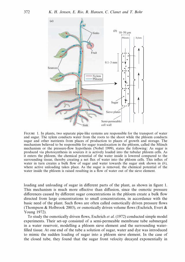
372 K. H. Jensen, E. Rio, R. Hansen, C. Clanet and T. Bohr
Sinks
Fruit
Sink
10–50 m
0.1–3 mm
Sugar
Sieve plates
Semi-permeablecell wall
Phloem Xylem
Xylem
Sources
Phloem
(a)
(b)
Figure 1. In plants, two separate pipe-like systems are responsible for the transport of waterand sugar. The xylem conducts water from the roots to the shoot while the phloem conductssugar and other nutrients from places of production to places of growth and storage. Themechanism believed to be responsible for sugar translocation in the phloem, called the Munchmechanism or the pressure-flow hypothesis (Nobel 1999), states the following: As sugar isproduced via photosynthesis in sources it is actively loaded into the tubular phloem cells. Asit enters the phloem, the chemical potential of the water inside is lowered compared to thesurrounding tissue, thereby creating a net flux of water into the phloem cells. This influx ofwater in turn creates a bulk flow of sugar and water towards the sugar sink shown in (b),where active unloading takes place. As the sugar is removed, the chemical potential of thewater inside the phloem is raised resulting in a flow of water out of the sieve element.
loading and unloading of sugar in different parts of the plant, as shown in figure 1.This mechanism is much more effective than diffusion, since the osmotic pressuredifferences caused by different sugar concentrations in the phloem create a bulk flowdirected from large concentrations to small concentrations, in accordance with thebasic need of the plant. Such flows are often called osmotically driven pressure flows(Thompson & Holbrook 2003), or osmotically driven volume flows (Eschrich, Evert &Young 1972).
To study the osmotically driven flows, Eschrich et al. (1972) conducted simple modelexperiments. Their set-up consisted of a semi-permeable membrane tube submergedin a water reservoir, modelling a phloem sieve element and the surrounding water-filled tissue. At one end of the tube a solution of sugar, water and dye was introducedto mimic the sudden loading of sugar into a phloem sieve element. In the case ofthe closed tube, they found that the sugar front velocity decayed exponentially in
126

Osmotically driven pipe flows and their relation to sugar transport in plants 373
time as it approached the far end of the tube. Also, they found the initial velocity ofthe sugar front to be proportional to concentration of the sugar solution. Throughsimple conservation arguments, they showed that for a flow driven according to thepressure-flow hypothesis, the velocity of the sugar front is given by
uf =L
t0exp
(− t
t0
)where t0 =
r
2κΠ, (1.1)
where t is time, L is the length of the sieve element and r its radius, κ is thepermeability of the membrane and Π is the osmotic pressure of the sugar solution.For dilute solutions, Π ≈ RT c (Landau & Lifshitz 1980), where R is the gas constant,T the absolute temperature and c the concentration in moles per volume. Theconservation argument for (1.1) is the following: for incompressible flow in a widerigid semi-permeable tube of length L imbedded in water, we imagine part of the tubeinitially filled with sugar solution and the rest with pure water. For a wide tube withslow flow, viscous effects and thus the pressure gradient along the tube is negligibleand the pressure is simply equal to the osmotic pressure Π averaged over the tube,i.e. RT c where c is the constant average sugar concentration. The water (volume)flux through the part of the tube ahead of the sugar front xf (where there is noosmosis) is −2πrκRT c(L − xf ), where κ is the permeability of the tube and the flowis negative since water flows out. This will be equal to the rate of change of volumeahead of xf and thus, due to incompressibility, is equal to −πr2dxf /dt . Putting thesetwo expressions together we get
dxf
dt=
2LpRT c
r(L − xf ) =
1
t0(L − xf ) (1.2)
leading to uf = dxf /dt given by (1.1).In the experiments performed by Eschrich et al. (1972) good qualitative agreement
with (1.1) was obtained, but on the quantitative level the agreement was rather poor.We thus chose to perform independent experiments along the same lines. Eschrich etal. (1972) used dye to track the sugar, and in one of our set-ups we can check thismethod by directly following the sugar without using dye. Also, we make independentmeasurements of the membrane properties, which then allow detailed comparison withthe predictions showing good quantitative agreement.
Simultaneously with the experiments, we develop the theory for osmotic flows. Theabove derivation of the front propagation is simplified by the lack of viscosity anddiffusion and, indeed, by the very assumption that a well-defined sugar front exists. Togo beyond this we must use the coupled equations for the velocity and concentrationfields as they vary along the tubes and in time. Here we follow the footsteps of a largenumber of authors, as discussed later. Our main contribution is the analysis of thedecay of an initially localized sugar concentration in a channel closed in both endsdescribed by (4.9) and (4.10). Here we point out that the main dimensionless number(termed as Munch number) can be chosen as
M =16ηL2κ
r3, (1.3)
where η is the fluid viscosity. We show how to simplify the equations and obtain exactsolutions in the regimes M � 1 (the regime of the experiments in this paper and ofthose of Eschrich et al.) and asymptotic solutions for M � 1. Both regimes are foundin plants and we propose an effective way for numerical integration of the equationsin the general case using Green’s functions. In the regime M � 1 the solubility of the
127

374 K. H. Jensen, E. Rio, R. Hansen, C. Clanet and T. Bohr
Quantity Magnitude Reference
Radius (μm) 4.5 (Fava bean), 4 (Winter Knoblauch & van Bel (1998),squash), 6–25 Taiz & Zeiger (2002),
Nobel (1999)Length (mm) 0.09 (Fava bean), 0.1–3 Knoblauch & van Bel (1998),
Nobel (1999)Flow velocity (m h−1) 0.5–1, 0.2–2 Knoblauch & van Bel (1998),
Nobel (1999)Elastic modulus (MPa) 17, 5.6–7.4 (Ash) Thompson & Holbrook (2003a),
Niklas (1992)Permeability (10−11 m s−1 Pa−1) 5,1.1 (Zitella translucence) Thompson & Holbrook (2003a),
Eschrich et al. (1972)Sucrose concentration (M)] 0.3–0.9 Taiz & Zeiger (2002)
Table 1. Characteristic properties of phloem sieve elements.
equations is shown by mapping them to a damped Burgers equation (5.6), which canbe solved by the method of characteristics. An analogous relation was pointed outearlier by Frisch (1976), but for a different boundary condition (open in one end)where the damping term disappears. Some results for M � 1 were also given by Weir(1981), but the lack of generality of his approach to the time-dependent problemmakes his results hard to extend.
In table 1 we show characteristic data for single sieve elements, which build up thephloem conducts in plants. If one naively applies these results to the flow inside suchsieve elements, taking L =1 mm, r =10 μm, κ = 10−11 m s−1 Pa−1 and concentrationc =0.5 M, one gets a characteristic velocity from (1.1) of 9 mh−1, almost an orderof magnitude larger than the range of velocities given in the table. Here one hasto remember that the characteristic velocity from (1.1) is valid for a transient flowcaused by an initial sudden sugar loading, whereas the velocities quoted in thetable are characteristic for the normal steady-state operation of the plants. For largedistances (e.g. those occurring in tall trees), the viscous effects embodied in (1.3)become large. Thus the value of M for the single sieve element considered aboveis M ≈ 1.6 × 10⁻⁴ whereas the value for a phloem tube spanning a distance of 10 mwould be greater by a factor 108, i.e. M ≈ 1.6 × 10⁴ (see also table 3 for characteristicvalues for M). In this regime (1.1) is no longer valid and, in fact, as seen in § 5.2 (5.46),the characteristic velocity will be reduced by a factor M−1/3, now making it an orderof magnitude smaller than the velocities quoted in the table. This seems to indicatethat large distance transport in trees cannot rely solely on the Munch mechanismand indeed the sieve elements are living cells and active transport may play a key role(see, e.g. Taiz & Zeiger 2002). For future studies in this direction it is important tobe able to separate these effects clearly and thus to understand the passive osmoticcomponent as clearly and simply as possible, which is the aim of the present paper.
The layout of the paper is as follows: §§ 2 and 3 describe our experimental set-upsand the experimental results obtained. In § 4, the flow equations are developed andin § 5 we present solutions for the cases M � 1 and M � 1. Finally, § 6 containsa detailed comparison between theory and experiments. After the conclusions (§ 7),two appendices follow. Appendix A provides information about the experimentalmaterials used and appendix B discusses the numerical methods (based on Green’sfunctions) used for solving the flow equations in the general case.
128

Osmotically driven pipe flows and their relation to sugar transport in plants 375
pt
ber
gt
(a)
(b)
spm
10 mm
spm
gtsswr
30 mmss
l
L30 cm wr
sc
ds
rs
Figure 2. Set-up I used to observe the movement of a sugar–dye solution (ss) inside asemi-permeable membrane tube (spm). L: length of membrane tube; l: initial sugar frontheight; ds: disposable syringe; gt: glass tube; rs: rubber stopper; sc: stopcock; wr: waterreservoir; bc: brass cylinder; pt: pressure transducer.
2. First experimental set-up
2.1. Set-up and methods
Set-up I is presented in figure 2. It is based on the design by Eschrich et al. withthe addition of a pressure transducer that allows us to measure the gauge pressure
129
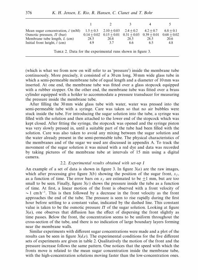
376 K. H. Jensen, E. Rio, R. Hansen, C. Clanet and T. Bohr
1 2 3 4 5
Mean sugar concentration, c (mM) 1.5 ± 0.3 2.10 ± 0.03 2.4 ± 0.2 4.2 ± 0.7 6.8 ± 0.1Osmotic pressure, Π (bar) 0.14 ± 0.02 0.15 ± 0.01 0.31 ± 0.03 0.39 ± 0.01 0.68 ± 0.02Membrane tube length, L (cm) 28.5 20.8 28.5 28.5 20.6Initial front height, l (cm) 4.9 3.7 6.6 6.5 4.8
Table 2. Data for the experimental runs shown in figure 3.
(which is what we from now on will refer to as ‘pressure’) inside the membrane tubecontinuously. More precisely, it consisted of a 30 cm long, 30 mm wide glass tube inwhich a semi-permeable membrane tube of equal length and a diameter of 10 mm wasinserted. At one end, the membrane tube was fitted over a glass stopcock equippedwith a rubber stopper. On the other end, the membrane tube was fitted over a brasscylinder equipped with a holder to accommodate a pressure transducer for measuringthe pressure inside the membrane tube.
After filling the 30 mm wide glass tube with water, water was pressed into thesemi-permeable tube with a syringe. Care was taken so that no air bubbles werestuck inside the tube. For introducing the sugar solution into the tube, a syringe wasfilled with the solution and then attached to the lower end of the stopcock which waskept closed. After fitting the syringe, the stopcock was opened and the syringe pistonwas very slowly pressed in, until a suitable part of the tube had been filled with thesolution. Care was also taken to avoid any mixing between the sugar solution andthe water already present in the semi-permeable tube. The physical characteristics ofthe membranes and of the sugar we used are discussed in appendix A. To track themovement of the sugar solution it was mixed with a red dye and data was recordedby taking pictures of the membrane tube at intervals of 15 min using a digitalcamera.
2.2. Experimental results obtained with set-up I
An example of a set of data is shown in figure 3. In figure 3(a) are the raw images,which after processing give figure 3(b) showing the position of the sugar front, xf ,as a function of time. The error bars on xf are estimated to be ±1 mm, but are toosmall to be seen. Finally, figure 3(c) shows the pressure inside the tube as a functionof time. At first, a linear motion of the front is observed with a front velocity of∼ 1 cmh−1. This is then followed by a decrease in the front velocity as the frontapproaches the end of the tube. The pressure is seen to rise rapidly during the firsthour before settling to a constant value, indicated by the dashed line. This constantvalue is taken to be the osmotic pressure Π of the sugar solution. Looking at figure3(a), one observes that diffusion has the effect of dispersing the front slightly astime passes. Below the front, the concentration seems to be uniform throughout thecross-section of the tube, and there is no indication of large boundary layers formingnear the membrane walls.
Similar experiments with different sugar concentrations were made and a plot of theresults can be seen in figure 3(d,e). The experimental conditions for the five differentsets of experiments are given in table 2. Qualitatively the motion of the front and thepressure increase follows the same pattern. One notices that the speed with which thefronts move is related to the mean sugar concentration inside the membrane tube,with the high-concentration solutions moving faster than the low-concentration ones.
130

Osmotically driven pipe flows and their relation to sugar transport in plants 377
20
15
10
5
0 42
t (h)
6 8 10 12
20.6 cm
0 42
10 20 30 40 50 60 70 80
6 8 10 12
x f (
cm)
25
20
15
10
5
5
5
43
21
413
2
0
10 20 30 40 50 60 70 800
x f (
cm)
0.8
0.6
0.4
0.2
p (b
ar)
0.8
0.6
0.4
0.2
p (b
ar)
(a)
(b)
(c)
(d)
(e)
Figure 3. Experimental results from set-up I. (a) Time series of pictures taken in experiment5. Time increases from left to right in steps of 30 min. See details of the sugar solutions usedin table 2. (b) Plot of the front position versus time obtained from the images above. (c) Plotof the gauge pressure inside the tube versus time. The dashed line is the osmotic pressure ofthe solution, taken to be the average value of the pressure from t = 2 h until the end of theexperiment. (d ) Plots of the sugar front position versus time for different sugar concentrations,as indicated in table 2. (e) Plots of the pressure inside the membrane tube for different sugarconcentrations.
131

378 K. H. Jensen, E. Rio, R. Hansen, C. Clanet and T. Bohr
(a)sg
sg
sg
Prism-
Top view
Side view
z
y
x
y
30 cm
7 cm
5 cm
Screen(b)
Semi-permeable membrane
Lase
r she
et
Water reservoir
Sugar solution
Water
Water reservoir
Water
Sugar solution
- Semi-permeable membrane
Water reservoir
x
y
z
Figure 4. Set-up II dedicated to the tracking of the sugar front via index of refraction changes.It consists of a hollow isosceles glass prism and a Plexiglas cuboid in osmotic contact througha membrane. A pressure transducer was attached to the top of the glass prism to measure thepressure inside.
The reason why 2 is moving slower than 1 is that experiment 2 was conducted in aslightly shorter membrane tube than the one used in experiment 1, thereby decreasingthe characteristic velocity as we shall see later.
3. Second experimental set-up
3.1. Set-up and methods
Set-up II is presented in figure 4. This set-up allows us to track the real front location,without the use of colorant, directly via the variation of the index of refraction.It consisted of a hollow isosceles glass prism and a Plexiglas cuboid in osmoticcontact through a membrane. To track the time evolution of the sugar front insidethe prism, we used the refraction of a laser sheet passing through it. The laser sheetwas generated by shining a laser beam, generated by a Melles Griot 3.1 mW laser,through a glass rod. When passing through the prism, light would deviate dependingon the local index of refraction, producing a typical S shape as shown in figure 4.The index of refraction varies linearly with sugar concentration and thus by lookingat the refracted laser sheet projected onto a screen, we were able to reconstruct theconcentration profile inside the prism. A camera recorded images of the screen atregular intervals to track the moving concentration profile.
132
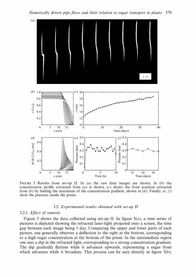
Osmotically driven pipe flows and their relation to sugar transport in plants 379
t →
5 10 150
0.2
0.4
0.6
0.8
1.0
(a)
(b)
(d) (e) ( f)
(c)
x (cm)
c (1
/c0)
5 10 150
0.2
0.4
0.6
x (cm)
dc/d
x [1
/(c 0
cm
)]
0 10 20 30 4010
12
14
16
18
20
Time (days)
x (c
m)
5 100
0.1
0.2
0.3
0.4
0.5
Pre
ssur
e (b
ar)
Time (h)32 34 36
0
0.1
0.2
0.3
0.4
0.5
Time (days)
Pre
ssur
e (b
ar)
Figure 5. Results from set-up II. In (a) the raw data images are shown. In (b) theconcentration profile extracted from (a) is shown. (c) shows the front position extractedfrom (b) by finding the maximum of the concentration gradient, shown in (d ). Finally, (e, f )show the pressure inside the prism.
3.2. Experimental results obtained with set-up II
3.2.1. Effect of osmosis
Figure 5 shows the data collected using set-up II. In figure 5(a), a time series ofpictures is depicted showing the refracted laser-light projected onto a screen, the timegap between each image being 1 day. Comparing the upper and lower parts of eachpicture, one generally observes a deflection to the right at the bottom, correspondingto a high sugar concentration at the bottom of the prism. In the intermediate regionone sees a dip in the refracted light, corresponding to a strong concentration gradient.The dip gradually flattens while it advances upwards, representing a sugar frontwhich advances while it broadens. This process can be seen directly in figure 5(b),
133
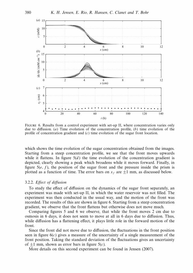
380 K. H. Jensen, E. Rio, R. Hansen, C. Clanet and T. Bohr
2 4 6 8 10 120
5
10
15
x (cm)
|dc/
dx| (
mM
cm
–1)
0 20 40 60 80 100 120 1404
5
6
7
t (h)
x f (
cm)
0 2 4 6 8 10 12
5
10
15(a)
(b)
(c)
x (cm)
c (m
M)
Figure 6. Results from a control experiment with set-up II, where concentration varies onlydue to diffusion. (a) Time evolution of the concentration profile, (b) time evolution of theprofile of concentration gradient and (c) time evolution of the sugar front location.
which shows the time evolution of the sugar concentration obtained from the images.Starting from a steep concentration profile, we see that the front moves upwardswhile it flattens. In figure 5(d ) the time evolution of the concentration gradient isdepicted, clearly showing a peak which broadens while it moves forward. Finally, infigure 5(e, f ), the position of the sugar front and the pressure inside the prism isplotted as a function of time. The error bars on xf are ±1 mm, as discussed below.
3.2.2. Effect of diffusion
To study the effect of diffusion on the dynamics of the sugar front separately, anexperiment was made with set-up II, in which the water reservoir was not filled. Theexperiment was then conducted in the usual way, and the motion of the front wasrecorded. The results of this are shown in figure 6. Starting from a steep concentrationgradient, we observe that the front flattens but otherwise does not move much.
Comparing figures 5 and 6 we observe, that while the front moves 2 cm due toosmosis in 6 days, it does not seem to move at all in 6 days due to diffusion. Thus,while diffusion has a flattening effect, it plays little role in the forward motion of thefront.
Since the front did not move due to diffusion, the fluctuations in the front positionseen in figure 6(c) gives a measure of the uncertainty of a single measurement of thefront position. Taking the standard deviation of the fluctuations gives an uncertaintyof ±1 mm, shown as error bars in figure 5(c).
More details on this second experiment can be found in Jensen (2007).
134
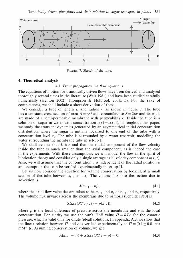
Osmotically driven pipe flows and their relation to sugar transport in plants 381
S
Ar
0 xi–lΔx
xf xi–l L
Water reservoir
Semi-permeable membrane
SugarWater flux
Figure 7. Sketch of the tube.
4. Theoretical analysis
4.1. Front propagation via flow equations
The equations of motion for osmotically driven flows have been derived and analysedthoroughly several times in the literature (Weir 1981) and have been studied carefullynumerically (Henton 2002; Thompson & Holbrook 2003a, b). For the sake ofcompleteness, we shall include a short derivation of these.
We consider a tube of length L and radius r , as shown in figure 7. The tubehas a constant cross-section of area A= πr2 and circumference S = 2πr and its wallsare made of a semi-permeable membrane with permeability κ . Inside the tube is asolution of sugar in water with concentration c(x) = c(x, t). Throughout this paper,we study the transient dynamics generated by an asymmetrical initial concentrationdistribution, where the sugar is initially localized to one end of the tube with aconcentration level c0. The tube is surrounded by a water reservoir, modelling thewater surrounding the membrane tube in set-up I.
We shall assume that L � r and that the radial component of the flow velocityinside the tube is much smaller than the axial component, as is indeed the casein the experiments. With these assumptions, we will model the flow in the spirit oflubrication theory and consider only a single average axial velocity component u(x, t).Also, we will assume that the concentration c is independent of the radial position ρ
an assumption that can be verified experimentally in set-up II.Let us now consider the equation for volume conservation by looking at a small
section of the tube between xi−1 and xi . The volume flux into the section due toadvection is
A(ui−1 − ui), (4.1)
where the axial flow velocities are taken to be ui−1 and ui at xi−1 and xi , respectively.The volume flux inwards across the membrane due to osmosis (Schultz 1980) is
S�xκ(RT c(x, t) − p(x, t)), (4.2)
where p is the local difference of pressure across the membrane and c is the localconcentration. For clarity we use the van’t Hoff value Π = RT c for the osmoticpressure, which is valid only for dilute (ideal) solutions. In appendix A.3, we show thatthe linear relation between Π and c is verified experimentally as Π = (0.1 ± 0.01 barmM−1)c. Assuming conservation of volume, we get
A(ui−1 − ui) + S�xκ(RT c − p) = 0. (4.3)
135

382 K. H. Jensen, E. Rio, R. Hansen, C. Clanet and T. Bohr
Letting �x → 0 and using that the cross-section to perimeter ratio reduces to r/2, thisbecomes
r
2
∂u
∂x= κ(RT c − p). (4.4)
For these very slow and slowly varying flows, the time dependence of the Navier–Stokes equation can be neglected and the velocity field is determined by theinstantaneous pressure gradient through the Poiseuille or Darcy relation (for a circulartube)
u = − r2
8η
∂p
∂x, (4.5)
where η is the dynamic viscosity of the solution, typically ∼ 1.5 × 10⁻³ Pa s in ourexperiments.
Differentiating (4.4) with respect to x and inserting the result from (4.5) we get forthe conservation of water that
RT∂c
∂x=
r
2κ
∂2u
∂x2− 8η
r2u. (4.6)
The final equation expresses the conservation of sugar advected with velocity u anddiffusing with molecular diffusivity D
∂c
∂t+
∂uc
∂x= D
∂2c
∂x2. (4.7)
The set of equations (4.6) and (4.7) is equivalent to those of Thompson & Holbrook(2003b) except for the fact that we have removed the pressure by substitution, andthat we do not consider elastic deformations of the tube.
4.1.1. Non-dimensionalization of the flow equations
To non-dimensionalize (4.6) and (4.7), we introduce the following scaling
c = c0C, u = u0U, x = LX, t = t0τ,
L has been chosen such that the spatial domain is now of the unit interval X ∈ [0, 1],u0 = L/t0 and c0 is the initial concentration level in one end of the tube. Choosingfurther
t0 =r
2κRT c0
, M =16ηL2κ
r3and D =
D
u0L=
Dr
2RT c0L2κ, (4.8)
and inserting in (4.6) and (4.7), we get the non-dimensional flow equations
∂2U
∂X2− MU =
∂C
∂X, (4.9)
∂C
∂τ+
∂UC
∂X= D
∂2C
∂X2. (4.10)
The parameter M corresponds to the ratio of axial to membrane flow resistance,which we shall refer to as the Munch number. This is identical to the parameter F inThompson & Holbrook (2003b). The second parameter D is the Peclet number. Thus,the longer the tube the less important the diffusion becomes and the more importantthe pressure gradient due to viscous effects becomes.
Values of the parameters M and D in different situations can be seen in table 3.The typical magnitude of the parameters M and D in plants are found from the
136

Osmotically driven pipe flows and their relation to sugar transport in plants 383
M D
Set-up I 2 × 10⁻⁸ 6 × 10⁻⁵
Set-up II 10−9 2 × 10⁻²
Single sieve element (L= 1 mm) 5 × 10⁻⁴ 5 × 10⁻⁴
Leaf (L= 1 cm) 5 × 10⁻² 5 × 10⁻⁵
Branch (L = 1 m) 5 × 10² 5 × 10⁻⁷
Small tree (L = 10 m) 5 × 10⁴ 5 × 10⁻⁸
Table 3. Values of the parameters M and D in various situations.
following values (also given in table 3):
r = 10 μm, η = 1.5 × 10⁻³ Pa s, u0 = 2 m h−1, κ = 2 × 10⁻¹¹ m (Pa s)−1.
We observe, that M and D are small in both experiments, and that for short distancetransport in plants this is also the case. However, over length scales comparable to abranch (L = 1 m) or a small tree (L = 10 m) M is large, so in this case the pressuregradient is not negligible.
When deriving the equations for osmotically driven flows, we have assumed thatthe concentration inside the tube was a function of x and t only. However, the realconcentration inside the tube will also depend on the radial position ρ in the formof a concentration boundary layer near the membrane, in the literature called anunstirred layer (Pedley 1983). Close to the membrane, the concentration cm is loweredcompared to the bulk value cb because sugar is advected away from the membraneby the influx of water. This, in turn, results in a lower influx of water, ultimatelycausing the axial flow inside the tube to be slower than expected. In our experimentswe see no signs of such boundary layers and apparently their width and their effecton the bulk flow are very small.
5. Solutions of the flow equations
We will now analyse (4.9) and (4.10). We will show that they can be solved quitegenerally for M = D = 0 by the method of characteristics. For an arbitrary initialcondition, this method will generally yield an implicit solution.
For arbitrary values of M and D, we cannot solve the equations of motionanalytically and thus have to incorporate numerical methods. This topic has been thefocus of much work both in the steady-state case (Thompson & Holbrook 2003a)and in the transient case (Henton 2002). However, no formulation fully exploiting thepartially linear character of the equations capable of handling all different boundaryconditions has so far been presented. Therefore, we show that using Green’s functions,the equations of motion can be transformed into a single integro-differential equation,which can be solved using standard numerical methods with very high precision. Thistechnical numerical part is detailed in appendix B.
5.1. Results for small Munch number
In the limit M = D =0 the equations become
∂2U
∂X2=
∂C
∂X, (5.1)
∂C
∂τ+
∂UC
∂X= 0. (5.2)
137

384 K. H. Jensen, E. Rio, R. Hansen, C. Clanet and T. Bohr
By integrating (5.1) with respect to X, we get
∂U
∂X= C + F (τ ). (5.3)
If we choose U (0) = U (1) = 0, F (τ ) becomes
F (τ ) = −∫ 1
0
C dX ≡ −C(τ ). (5.4)
Using (5.3) in (5.2) gives
∂
∂X
[∂U
∂τ+ U
(∂U
∂X+ C
)]= −dC
dτ= 0, (5.5)
where the last equality follows from integrating X from 0 to 1, observing that allterms in the square bracket vanish at the end points due to the boundary conditionu(X =0, τ ) = u(X = 1, τ ) = 0. Thus C is a constant in time since the tube is closed.Integrating with respect to X and using the boundary conditions on U , this becomes
∂U
∂τ+ U
∂U
∂X= −CU. (5.6)
Equation (5.6) is a damped Burgers equation (Gurbatov, Malakhov & Saichev 1991),which can be solved using Riemann’s method of characteristics. The characteristicequations are
dU
dτ= −CU (5.7)
dX
dτ= U. (5.8)
Equation (5.7) has the solution
U = U0(ξ ) exp(−Cτ ), (5.9)
where the parametrization ξ (X, τ ) of the initial velocity has to be found from
X = ξ +1
CU0(ξ )(1 − exp(−Cτ )), (5.10)
where ξ = X at τ =0.
5.1.1. Exact solutions for simple initial conditions
An experimental condition close to that of our experiments is to use a Heavisidestep function as initial condition on C, making C initially constant in some interval[0, λ]
C(X, τ = 0) = CIH (λ − X) =
{CI for 0 � X � λ.
0 for λ < X � 1.(5.11)
Equation (5.3) now enables us to find the initial condition on the velocity
U (X, τ = 0) =
∫ X
0
(C(X′, 0) − C) dX′ =
∫ X
0
(C(X′, 0) − λCI ) dX′ (5.12)
=
{(CI − C)X for 0 � X � λ.
C(1 − X) for λ < X � 1.(5.13)
138
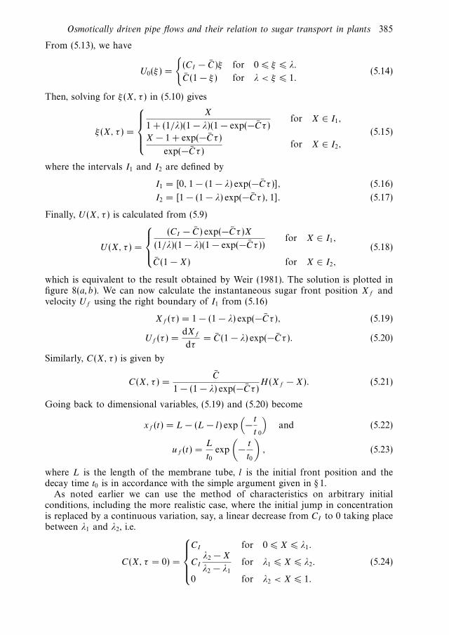
Osmotically driven pipe flows and their relation to sugar transport in plants 385
From (5.13), we have
U0(ξ ) =
{(CI − C)ξ for 0 � ξ � λ.
C(1 − ξ ) for λ < ξ � 1.(5.14)
Then, solving for ξ (X, τ ) in (5.10) gives
ξ (X, τ ) =
⎧⎪⎪⎨⎪⎪⎩
X
1 + (1/λ)(1 − λ)(1 − exp(−Cτ )for X ∈ I1,
X − 1 + exp(−Cτ )
exp(−Cτ )for X ∈ I2,
(5.15)
where the intervals I1 and I2 are defined by
I1 = [0, 1 − (1 − λ) exp(−Cτ )], (5.16)
I2 = [1 − (1 − λ) exp(−Cτ ), 1]. (5.17)
Finally, U (X, τ ) is calculated from (5.9)
U (X, τ ) =
⎧⎪⎨⎪⎩
(CI − C) exp(−Cτ )X
(1/λ)(1 − λ)(1 − exp(−Cτ ))for X ∈ I1,
C(1 − X) for X ∈ I2,
(5.18)
which is equivalent to the result obtained by Weir (1981). The solution is plotted infigure 8(a, b). We can now calculate the instantaneous sugar front position Xf andvelocity Uf using the right boundary of I1 from (5.16)
Xf (τ ) = 1 − (1 − λ) exp(−Cτ ), (5.19)
Uf (τ ) =dXf
dτ= C(1 − λ) exp(−Cτ ). (5.20)
Similarly, C(X, τ ) is given by
C(X, τ ) =C
1 − (1 − λ) exp(−Cτ )H (Xf − X). (5.21)
Going back to dimensional variables, (5.19) and (5.20) become
xf (t) = L − (L − l) exp(
− t
t 0
)and (5.22)
uf (t) =L
t0exp
(− t
t0
), (5.23)
where L is the length of the membrane tube, l is the initial front position and thedecay time t0 is in accordance with the simple argument given in § 1.
As noted earlier we can use the method of characteristics on arbitrary initialconditions, including the more realistic case, where the initial jump in concentrationis replaced by a continuous variation, say, a linear decrease from CI to 0 taking placebetween λ1 and λ2, i.e.
C(X, τ = 0) =
⎧⎪⎪⎨⎪⎪⎩
CI for 0 � X � λ1.
CI
λ2 − X
λ2 − λ1
for λ1 � X � λ2.
0 for λ2 < X � 1.
(5.24)
139

386 K. H. Jensen, E. Rio, R. Hansen, C. Clanet and T. Bohr
0.5 1.00
0.2
0.4
0.6
0.8
1.0(a) (b)
(c) (d)
0.5 1.00
0 00.5 1.0
X
0.5 1.0
X
C
0.05
0.10
U
0.2
0.4
0.6
0.8
1.0
C
0.05
0.10
U
Figure 8. (a, b) Plot of the analytical solution for a piecewise constant initial concentration.λ=0.1, CI = 1 and C = 0.1. (c, d) Plot of the analytical solution for a piecewise linear initialconcentration. λ1 = 0.05, λ2 = 0.15, CI = 1 and C = 0.1. Time increases from black to gray insteps of one unit of time.
Using (5.3) yields the initial velocity
U (X, τ = 0) =
⎧⎪⎨⎪⎩
(CI − C)X for 0 � X � λ1,
A1X2 + B1X + C1 for λ1 � X � λ2,
C(1 − X) for λ2 < X � 1,
(5.25)
where C = CI (λ1 + λ2)/2, and the constants are given by
A1 = − CI
2(λ2 − λ1), B1 =
CIλ2
λ2 − λ1
− C, C1 = CIλ1 +CI
λ2 − λ1
(λ1λ2 + λ2
1/2). (5.26)
Finding ξ (X, τ ) from (5.10) now gives
ξ (X, τ ) =
⎧⎪⎪⎪⎪⎪⎪⎨⎪⎪⎪⎪⎪⎪⎩
X
1 + (1/λ)(1 − λ)(1 − exp(−Cτ )for X ∈ I1,
A2ξ22 + B2ξ
22 + C2 for X ∈ I2,
X − 1 + exp(−Cτ )
exp(−Cτ )for X ∈ I3,
(5.27)
where
A2 =A1
C(1 − exp(−Cτ )), B2 = 1 +
B1
C(1 − exp(−Cτ )), C2 =
C1
C(1 − exp(−Cτ )).
(5.28)
140
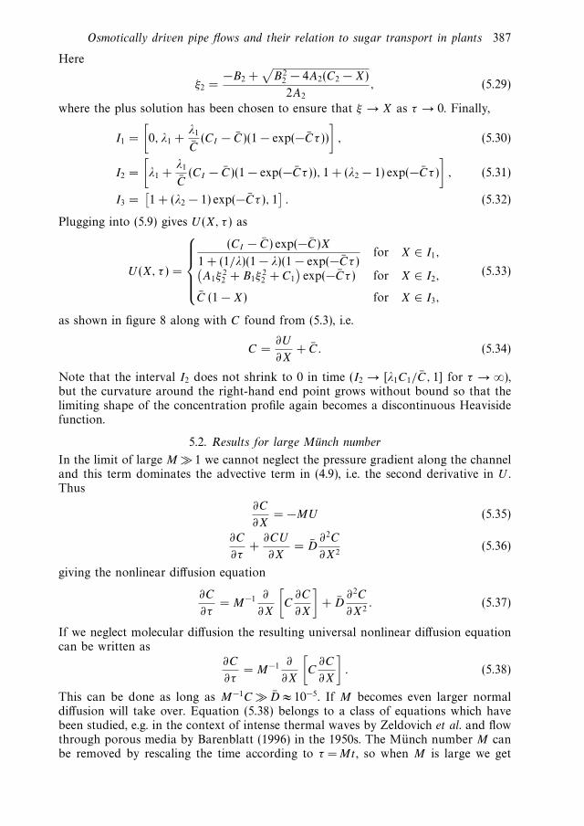
Osmotically driven pipe flows and their relation to sugar transport in plants 387
Here
ξ2 =−B2 +
√B2
2 − 4A2(C2 − X)
2A2
, (5.29)
where the plus solution has been chosen to ensure that ξ → X as τ → 0. Finally,
I1 =
[0, λ1 +
λ1
C(CI − C)(1 − exp(−Cτ ))
], (5.30)
I2 =
[λ1 +
λ1
C(CI − C)(1 − exp(−Cτ )), 1 + (λ2 − 1) exp(−Cτ )
], (5.31)
I3 =[1 + (λ2 − 1) exp(−Cτ ), 1
]. (5.32)
Plugging into (5.9) gives U (X, τ ) as
U (X, τ ) =
⎧⎪⎪⎪⎨⎪⎪⎪⎩
(CI − C) exp(−C)X
1 + (1/λ)(1 − λ)(1 − exp(−Cτ )for X ∈ I1,(
A1ξ22 + B1ξ
22 + C1
)exp(−Cτ ) for X ∈ I2,
C (1 − X) for X ∈ I3,
(5.33)
as shown in figure 8 along with C found from (5.3), i.e.
C =∂U
∂X+ C. (5.34)
Note that the interval I2 does not shrink to 0 in time (I2 → [λ1C1/C, 1] for τ → ∞),but the curvature around the right-hand end point grows without bound so that thelimiting shape of the concentration profile again becomes a discontinuous Heavisidefunction.
5.2. Results for large Munch number
In the limit of large M � 1 we cannot neglect the pressure gradient along the channeland this term dominates the advective term in (4.9), i.e. the second derivative in U .Thus
∂C
∂X= −MU (5.35)
∂C
∂τ+
∂CU
∂X= D
∂2C
∂X2(5.36)
giving the nonlinear diffusion equation
∂C
∂τ= M−1 ∂
∂X
[C
∂C
∂X
]+ D
∂2C
∂X2. (5.37)
If we neglect molecular diffusion the resulting universal nonlinear diffusion equationcan be written as
∂C
∂τ= M−1 ∂
∂X
[C
∂C
∂X
]. (5.38)
This can be done as long as M−1C � D ≈ 10−5. If M becomes even larger normaldiffusion will take over. Equation (5.38) belongs to a class of equations which havebeen studied, e.g. in the context of intense thermal waves by Zeldovich et al. and flowthrough porous media by Barenblatt (1996) in the 1950s. The Munch number M canbe removed by rescaling the time according to τ = Mt , so when M is large we get
141
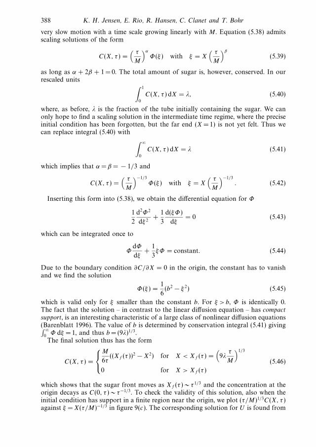
388 K. H. Jensen, E. Rio, R. Hansen, C. Clanet and T. Bohr
very slow motion with a time scale growing linearly with M . Equation (5.38) admitsscaling solutions of the form
C(X, τ ) =( τ
M
)α
Φ(ξ ) with ξ = X( τ
M
)β
(5.39)
as long as α + 2β + 1 = 0. The total amount of sugar is, however, conserved. In ourrescaled units ∫ 1
0
C(X, τ ) dX = λ, (5.40)
where, as before, λ is the fraction of the tube initially containing the sugar. We canonly hope to find a scaling solution in the intermediate time regime, where the preciseinitial condition has been forgotten, but the far end (X = 1) is not yet felt. Thus wecan replace integral (5.40) with ∫ ∞
0
C(X, τ ) dX = λ (5.41)
which implies that α = β = − 1/3 and
C(X, τ ) =( τ
M
)−1/3
Φ(ξ ) with ξ = X( τ
M
)−1/3
. (5.42)
Inserting this form into (5.38), we obtain the differential equation for Φ
1
2
d2Φ2
dξ 2+
1
3
d(ξΦ)
dξ= 0 (5.43)
which can be integrated once to
ΦdΦ
dξ+
1
3ξΦ = constant. (5.44)
Due to the boundary condition ∂C/∂X = 0 in the origin, the constant has to vanishand we find the solution
Φ(ξ ) =1
6(b2 − ξ 2) (5.45)
which is valid only for ξ smaller than the constant b. For ξ > b, Φ is identically 0.The fact that the solution – in contrast to the linear diffusion equation – has compactsupport, is an interesting characteristic of a large class of nonlinear diffusion equations(Barenblatt 1996). The value of b is determined by conservation integral (5.41) giving∫ ∞
0Φ dξ = 1, and thus b = (9λ)1/3.
The final solution thus has the form
C(X, τ ) =
⎧⎨⎩
M
6τ((Xf (τ ))2 − X2) for X < Xf (τ ) =
(9λ
τ
M
)1/3
0 for X > Xf (τ )
(5.46)
which shows that the sugar front moves as Xf (τ ) ∼ τ 1/3 and the concentration at theorigin decays as C(0, τ ) ∼ τ−1/3. To check the validity of this solution, also when theinitial condition has support in a finite region near the origin, we plot (τ/M)1/3C(X, τ )against ξ =X(τ/M)−1/3 in figure 9(c). The corresponding solution for U is found from
142

Osmotically driven pipe flows and their relation to sugar transport in plants 389
0.5 1.0
(a)
(b)
(c)
0.2
0.4
0.6
0.8
1.0
X
0.5 1.0X
C
0
0
0.2
0.4
0.6
0.8
1.0
CM = 100
0.5 1.0 1.50
0.02
0.04
0.06
0.08
0.10
0.12
0.14
0.16
0.18
0.20
ξ
(Mτ)
1/3
C
1/6(b2 – ξ2)
Figure 9. (a) Numerical simulation of (5.38) compared with (b) scaling solution (5.46) and(c) (5.45), which is shown as a dashed line. The initial condition has the form C(X, 0) =1 − [1 + exp(−(X − λ)/ε)]−1, where λ= 0.1 and ε = 2 × 10⁻² and the curves are equidistant intime. When λ controlling the size of the region of non-zero initial sugar concentration becomeslarger, a more accurate scaling solution is found by letting τ → τ + τ0 and treating τ0 as anunknown parameter. In (c), we have omitted the first curve (the initial condition).
(5.35) as
U (X, τ ) =
⎧⎨⎩
X
3τfor X < Xf (τ )
0 for X > Xf (τ )
(5.47)
and ∂2U/∂X2 = 0 justifying the neglect of ∂2U/∂X2 in going from (4.9) to (5.35) forlarge M . It is seen that the velocity of the sugar front X′
f (τ ) = (λ/(3M))1/3τ−2/3 isidentical to U (Xf (τ ), τ ) from (5.47).
6. Comparison between theory and experiment
In §§ 2.2 and 3.2, we have presented experiments demonstrating the movement of asugar solution inside a membrane tube surrounded by a reservoir of water. We nowwish to consider whether the theory is in agreement with the experimental results.
6.1. Set-up I
The plot in figure 10 shows the relative front position, (L − xf )/(L − l), plottedagainst time for five different experiments conducted with set-up I. The numbers 1–5indicate the sugar concentrations used (cf. table 2). One clearly sees, that the relativefront position approaches zero faster for high concentrations than for low. Typical
143
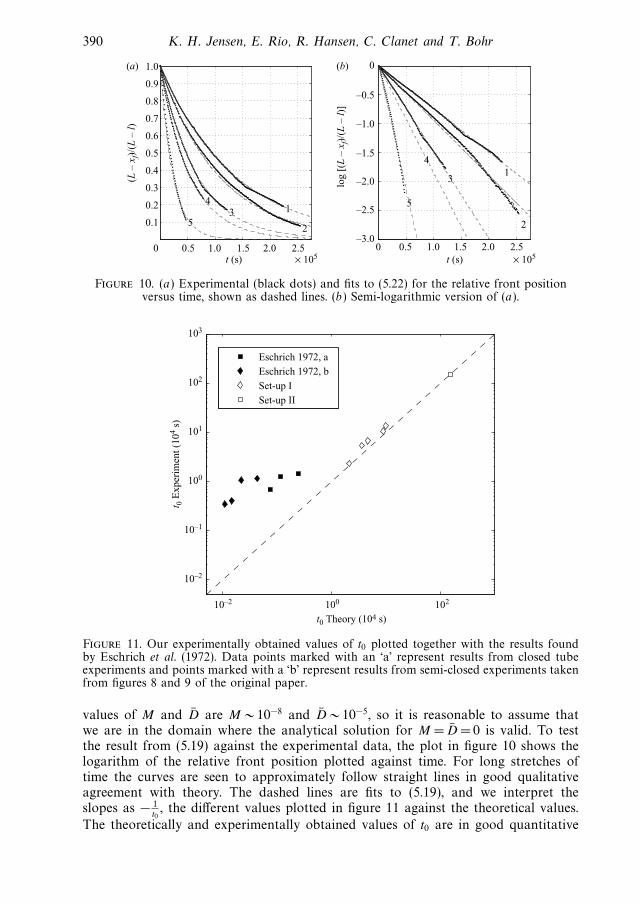
390 K. H. Jensen, E. Rio, R. Hansen, C. Clanet and T. Bohr
0.5 1.0 1.5 2.0 2.5× 10⁵
0
0.1
0.2
0.3
0.4
0.5
0.6
0.7
0.8
0.9
1.0
4
(L –
xf)/
(L –
l)
log
[(L
– x
f)/(L
– l)
]
t (s) × 105t (s)
2
135
0 0.5 1.0 1.5 2.0 2.5
0(a) (b)
–0.5
–1.0
–1.5
–2.0
–2.5
–3.0
4
2
13
5
Figure 10. (a) Experimental (black dots) and fits to (5.22) for the relative front positionversus time, shown as dashed lines. (b) Semi-logarithmic version of (a).
10–2
10–2 100 102
10–1
100
101
102
103
t0 Theory (104 s)
t 0 E
xper
imen
t (10
4 s)
Eschrich 1972, a
Eschrich 1972, b
Set-up I
Set-up II
Figure 11. Our experimentally obtained values of t0 plotted together with the results foundby Eschrich et al. (1972). Data points marked with an ‘a’ represent results from closed tubeexperiments and points marked with a ‘b’ represent results from semi-closed experiments takenfrom figures 8 and 9 of the original paper.
values of M and D are M ∼ 10−8 and D ∼ 10−5, so it is reasonable to assume thatwe are in the domain where the analytical solution for M = D = 0 is valid. To testthe result from (5.19) against the experimental data, the plot in figure 10 shows thelogarithm of the relative front position plotted against time. For long stretches oftime the curves are seen to approximately follow straight lines in good qualitativeagreement with theory. The dashed lines are fits to (5.19), and we interpret theslopes as − 1
t0, the different values plotted in figure 11 against the theoretical values.
The theoretically and experimentally obtained values of t0 are in good quantitative
144

Osmotically driven pipe flows and their relation to sugar transport in plants 391
10 20 30 400
0.2
0.4
0.6
0.8
1.0
1.2
t (days) t (days)0 10 20 30 40
(L –
xf)/
(L –
l)
log
[(L
– x
f)/(L
– l)
]
(b)(a) –0.5
–0.5
0
–1.5
–2.0
–2.5
–3.5
–3.0
–1.0
Figure 12. (a) Experimental data obtained using set-up II showing the relative front position(black dots) as a function of time. (b) Lin–log plot of the experimental data shown on the left.The solid line is a fit to (5.22) with t0 = 1.6 × 10⁶ s.
agreement, within 10 %–30 %. Generally, theory predicts somewhat smaller valuesof t0 than observed, implying that the observed motion of the sugar front is a littleslower than expected from the pressure-flow hypothesis. Nevertheless, as can beseen in figure 11 these results are a considerable improvement to the previous resultsobtained by Eschrich et al. as we find much better agreement between experiment andtheory.
6.2. Set-up II
The plot in figure 12 shows the relative front position, (L − xf )/(L − l), plottedagainst time for the experiment conducted with set-up I. On the semi-logarithmicplot, the curves are seen to follow straight lines in good qualitative agreement withthe simple theory for M = D = 0. As can be seen in figure 11, we also found verygood quantitative agreement between the experiment and theory for set-up II.
To test how well the motion of the sugar front observed in the experiments with set-up II was reproduced by our model, we solved the equations of motion numericallystarting with the initial conditions from figure 5. For M = D = 0, the results are shownin figure 13(b). While the front positions are reproduced relatively well, the shapeof the front is not, so diffusion must play a role. This can be seen in figure 13(c)which shows the result of simulation with M = 10−9, D = 6.9 × 10⁻¹¹ m2 s−1. Clearly,the model which includes diffusion reproduces the experimental data significantlybetter.
To study the shape of the front in greater detail, consider the plots in figure 13(d–f ).Here the gradient of the concentration curves on the left in figure 13 is shown. Infigure 13(d ) we clearly see a peak moving from left to right while it gradually broadensand flattens. In figure 13(e) also we see the peak advancing, but the flattening andbroadening is much less pronounced. In figure 13(f ) we see that the model whichincludes diffusion reproduces the gradual broadening and flattening of the front verywell.
7. Conclusion
In this paper we have studied osmotically driven transient pipe flows. The flowsare generated by concentration differences of sugar in closed tubes, fully or partly
145

392 K. H. Jensen, E. Rio, R. Hansen, C. Clanet and T. Bohr
2 4 6 8 10 120
5
10
15(a)
(b)
(c)
(d)
(e)
(f)
2 4 6 8 10 120
5
10
15
2 4 6 8 10 120
5
10
15
2 4 6 8 10 120x (cm)
c (m
M)
2 4 6 8 10 120
5
10
15
2 4 6 8 10 120
5
10
15
5
10
15
|dc/
dx| (
mM
cm
–1)
Figure 13. Results from set-up II showing the experimental data (a, d ) and the numericalmodel for M = D = 0 (b, e) and for M = 10−9, D = 6.9 × 10⁻¹¹ m2 s−1 (c, f ).
enclosed by semi-permeable membranes surrounded by pure water. The flows areinitiated by a large concentration in one end of the tube and we study the approachto equilibrium, where the sugar is distributed evenly within the tube. Experimentally,we have used two configurations: the first is an updated version of the set-up ofEschrich et al. where the flow takes place in a dialysis tube and the sugar is followedby introducing a dye. The advantage is the relatively rapid motion, due to the largesurface area. The disadvantage is that the sugar concentration cannot be inferredaccurately by this method and for this reason we have introduced our second set-up,where the sugar concentration can be followed directly by refraction measurements.
On the theoretical side, we first re-derive the governing flow equations and introducethe dimensionless Munch number M . We then show that analytical solutions can beobtained in the two important limits of very large and very small M . In the generalcase we show how numerical methods based on Green’s functions are very effective.
146

Osmotically driven pipe flows and their relation to sugar transport in plants 393
Finally, we compare theory and experiment with very good agreement. In particularthe results or the velocity of the front (as proposed by Eschrich et al.) can be verifiedrather accurately.
Concerning the application to sap flow, the quantitative study we performed leadsto the following conclusions: for a large tree it seems improbable that sugar transport,e.g. from leaf to root by this sole passive mechanism would be sufficiently efficient. Inthis case active transport processes might play an important role. On the other hand,transport over short distances, e.g. locally in leaves or from a leaf to a nearby shootmight be more convincingly described by the pressure-flow hypothesis.
It is a pleasure to thank Francois Charru, Marie-Alice Goudeau-Boudeville, HervCochard, Pierre Cruiziat, Alexander Schulz, N. Michele Holbrook and VakhtangPutkaradze for many useful discussions. Much appreciated technical assistance wasprovided by Erik Hansen. This work was supported by the Danish National ResearchFoundation, Grant No. 74.
Appendix A. Materials: sugar and membrane
A.1. Sugar
The sugar used was a dextran (Sigma-Aldrich, St Louis, MO, USA, type D4624)with an average molecular weight of 17.5 kDa. The dye used was a red fruit dye(Flachsmann Scandinavia, Rød Frugtfarve, type 123000) consisting of an aqueousmixture of the food additives E-124 and E-131 with molecular weights of 539 Daand 1159 Da, respectively (PubChem-Database 2007). Even though the molecularweights are below the MWCO of the membrane, the red dye was not observed toleak through the membrane. This, however, was observed when using another type ofdye, Methylene blue, which has a molecular weight of 320 Da.
A.2. Membrane
The membrane used in both set-ups was a semi-permeable dialysis membrane tube(Spectra/Por Biotech cellulose ester dialysis membrane) with a radius of 5 mm,a thickness of 60 μm and a MWCO (molecular weight cut off) of 3.5 kDa. Thepermeability Lp was determined by applying a pressure and measuring the flow rateacross the membrane
Lp = (1.8 ± 0.2) × 10−12 m (Pa s)−1. (A 1)
A.3. Osmotic strength of dextran
Figure 14(left) shows the relation between dextran concentration and osmotic pressurefound from the experiments shown in figure 3. A linear fit gives
Π = (0.1 ± 0.01 bar mM−1)c (A 2)
where Π has unit bar, and c is measured in mM. This is in good agreement withvalues given by Jonsson (1986).
Appendix B. Numerical methods for non-zero M and D
For non-zero values of M and D, the equations of motion,
∂2U
∂X2− MU =
∂C
∂X(B 1)
147

394 K. H. Jensen, E. Rio, R. Hansen, C. Clanet and T. Bohr
1 2 3 4 5 6 70
0.1
0.2
0.3
0.4
0.5
0.6
0.7
0.8
c (mM)
Osm
otic
pre
ssur
e, Π
(ba
r)
Figure 14. van’t Hoff relation for 17.5 kDa dextran.
and
∂C
∂τ+
∂CU
∂X= D
∂2C
∂X2(B 2)
cannot be solved analytically. However, they can be written as a single integro-differential equation, which is straightforward to solve on a computer. If we choosea set of linear boundary conditions, BX[U ] = ai , for (B 1), the solution can be writtenas
U =
∫ 1
0
G(X, ξ )∂C
∂ξdξ + U2. (B 3)
Here, G(X, ξ ) is the Green’s function for the differential operator ∂2/∂X2 − M withboundary conditions BX[U ] = 0 and U2 fulfils the homogeneous version of (B 1) withBX[U ] = ai . Plugging this into (B 2) yields
∂C
∂τ+
∂
∂X
(C
(∫ 1
0
G(X, ξ )∂C
∂ξdξ + U2
))= D
∂2C
∂X2. (B 4)
For the closed tube, i.e. for the boundary conditions U (0, τ ) = U (1, τ ) = 0, G(X, ξ ) isgiven by
G(X, ξ ) =
⎧⎪⎪⎨⎪⎪⎩
−sinh(a(1 − X))
a sinh asinh aξ for ξ < X,
−sinh aX
a sinh asinh(a(1 − ξ )) for ξ > X,
(B 5)
and U2 = 0. To increase numerical accuracy, it is convenient to transform (B 4) bydefining
∂f
∂X= C − C (B 6)
and choosing f (0) = f (1) = 0 such that f (X) =∫ X
0(C − C)dξ . Inserting in (B 4), we
get
∂f
∂t= D
∂2f
∂X2−
(f (X) −
∫ 1
0
∂K(X, ξ )
∂ξf (ξ )dξ
)(∂f
∂X+ C
), (B 7)
148

Osmotically driven pipe flows and their relation to sugar transport in plants 395
0 0.2 0.4 0.6 0.8
M = 0.01
M = 1
M = 10
1.0
0 0.2 0.4 0.6 0.8 1.0
0 0.2 0.4x x
0.6 0.8 1.0
0
0.05
0.10
0.15
0.20
0.05
0.10
0.15
0.20
0.05
0.10
0.15
0.20
0.2 0.4 0.6 0.8 1.0
0
0
0.2 0.4 0.6 0.8 1.0
0.2 0.4 0.6 0.8 1.0
0.2
0.4
0.6
0.8
1.0
0.2
0.4
0.6
0.8
1.0
0.2
0.4
0.6c U
0.8
1.0
Figure 15. Results of numerical simulation of (B 4) using the boundary conditions U (0, τ ) =U (1, τ ) = 0 for different values of M . D is kept constant at 10−5. The initial condition wasC(X, 0) = 1 − 1/(1 + exp(−(X − λ)/ε)) where λ= 0.2 and ε = 2 × 10².
where
∂K(X, ξ )
∂ξ=
⎧⎪⎨⎪⎩
−asinh(a(1 − X))
sinh asinh aξ for ξ < X,
−asinh aX
sinh asinh(a(1 − ξ )) for ξ > X.
(B 8)
To solve (B 7) we used Matlab’s built-in time solver ode23t which is based on anexplicit Runge–Kutta formula along with standard second-order schemes for the first-and second-order derivatives. For the spatial integration, the trapezoidal rule wasused (Press 2001). Results of a numerical simulation for different values of M areshown in figure 15.
REFERENCES
Barenblatt, G. I. 1996 Scaling, Self-Similarity, and Intermediate Asymptotics. Cambridge UniversityPress.
Eschrich, W., Evert, R. F. & Young, J. H. 1972 Solution flow in tubular semipermeable membranes.Planta(Berl.) 107, 279–300.
Frisch, H. L. 1976 Osmotically driven flow in narrow channels. Trans. Soc. Rheol. 20, 23–27.
Gurbatov, S. N. Malakhov, A. N. & Saichev, A. I. 1991 Nonlinear Random Waves and Turbulencein Nondispersive Media: Waves, Rays, Particles. Manchester University Press.
149
396 K. H. Jensen, E. Rio, R. Hansen, C. Clanet and T. Bohr
Henton, S. M. 2002 Revisiting the Munch pressure-flow hypothesis for long-distance transport ofcarbohydrates: modelling the dynamics of solute transport inside a semipermeable tube. J.Exp. Bot. 53, 1411–1419.
Jonsson, G. 1986 Transport phenomena in ultrafiltration: membrane selectivity and boundary layerphenomena. J. Pure Appl. Chem. 58, 1647–1656.
Jensen, K. H. 2007 Osmotically driven flows and their relation to sugar transport in plants. MScThesis, The Niels Bohr Institute, University of Copenhagen.
Knoblauch, M. & van Bel, A. J. E. 1998 Sieve tubes in action. The Plant Cell 10, 35–50.
Landau, L. D. & Lifshitz, E. M. 1980 Statistical Physics. Pergamon Press.
Munch, E. 1930 Die Stoffbewegung in der Pflanze. Verlag von Gustav Fisher.
Niklas, K. J. 1992 Plant Biomechanics – An Engineering Approach to Plant Form and Function. TheUniversity of Chicago Press.
Nobel, P. S. 1999 Physicochemical & Environmental Plant Physiology. Academic Press.
Pedley, T. J. 1983 Calculation of unstirred layer thickness in membrane transport experiments: asurvey. Quart. Rev. Biophys. 16, 115–150.
Press, W. H. 2001 Numerical Recipes in Fortran 77, Vol. 1 Cambridge University Press.
PubChem–Database 2007 http://pubchem.ncbi.nlm.nih.gov/ National Library of Medicine
Schultz, S. G. 1980 Basic Principles of Membrane Transport. Cambridge University Press.
Taiz, L. & Zeiger, E. 2002 Plant Physiology. Sinauer Associates.
Thompson, M. V. & Holbrook, N. M. 2003a, Application of a single-solute non-steady-state phloemmodel to the study of long-distance assimilate transport. J. Theor. Biol. 220, 419–455.
Thompson, M. V. & Holbrook, N. M. 2003b, Scaling phloem transport: water potential equilibriumand osmoregulatory flow. Plant, Cell Environ. 26, 1561–1577.
Weir, G. J. 1981 Analysis of Munch theory. Math. Biosci. 56, 141–152.
150

151

The Danish Polymer Centre
Department of Chemical and Biochemical Engineering
Technical University of Denmark
Søltofts Plads, Building 227
DK-2800 Kgs. Lyngby
Denmark
Phone: +45 4525 6801
Web: www.dpc.kt.dtu.dk
ISBN : 978-87-92481-75-7


