
The Voucher System and the Agricultural Production in Tanzania: Is the model adopted
effective? Evidence from the Panel Data analysis*
Aloyce S. Hepelwa†, Onesmo Selejio‡ and John K. Mduma§
August 2013
Abstract
One of the policy measures adopted in the recent past by the government of Tanzania during the
implementation of the Agricultural Sector Development Program (ASDP) is to subsidize the
fertilizer and other agricultural inputs through the National Agricultural Input Voucher system
(NAIVS). Poor smallholder farmers who are the beneficiaries of NAIVS are expected to increase
crop productivity per unit area and hence reduce extensive farming/shifting cultivation. This
paper presents empirical results on the effects of the NAIVS on crop production in some selected
regions in Tanzania. The study used the panel data analysis technique to analyze agricultural
data collected in year 2007(before NAIVS) and 2012 (during NAIVS). The study found a
statistically significant difference between crop harvest by households with and without access to
NAIVS. The average crop yield (production per area) is relatively higher in 2012 than the yield
in 2007. On average the area cultivated by the households has increased more than double in
2012. Majority poor smallholder farmers do not access the NAIVS due to high market price of
inputs not well compensated by the static low value NAIVS. Also the study found that the effect of
NAIVS is significantly high to the well off households. The implication from this finding is that
the NAIVS is not achieving the intended objective of increasing crop productivity by the poor
smallholders. NAIVS would have the desirable results when deliberate efforts to address the
institutional and market system shortfall are instituted.
* We acknowledge the financial support from the Swedish International Development Agency (Sida) through the Environment for Development Initiative (EfD) of the Department of Economics, University of Dar es Salaam. † Department of Economics, University of Dar es Salaam, e-mail: [email protected] ‡‡Department of Economics, University of Dar es Salaam, e-mail: [email protected] § Department of Economics, University of Dar es Salaam, e-mail:[email protected]
Key Words: Fertilizer subsidy, crop productivity, Panel data analysis.
Introduction In Tanzania, agricultural sector is one of the key sectors to the national economy. Over
80% of the population lives in rural areas and their livelihoods depend on agriculture.
The sector accounts for 26.4% of the GDP, 30% of export earnings and 65% of raw
material for domestic industries (World Bank, 2010). Agriculture sector employs about
74 percent of the labour force (URT, 2007). However, the sector experience low growth.
Given the importance of the sector as a source income, employment and food security,
this low growth has translated into little progress on poverty reduction. The proportion
of people living below the basic needs poverty line remains high at more than 33% in
2007 (HBS, 2007). The 2007/2008 NSCA, the most recent agricultural census
approximates 12.6 million hectares of land to be the land under agricultural activities in
the country which includes both temporary and permanent crops as well as livestock
keeping. Smallholder farmers occupy 91% of the total area under agriculture. The
remaining 9% of the land is held by large scale farmers who own a total of 1.1 million
hectares**. The average food crop productivity in Tanzania stood at about 1.7 tons/ha
far below the potential productivity of about 3.5 to 4 ton/ha (Table 1). High
dependence on rainfall is the main characteristics of the agricultural practices by the
small holder farmers in the country. In addition, the crop cultivation is characterized by
low mechanization where majority farmers are using poor farm inputs such as hand
hoe and traditional seeds. The soils have been degraded with significant loss of
nutrients and thus contributing to low productivity problem.
** Large scale farms are considered to be the farms with size above 20 hectares (or 50 acres).

Table 1: Maize and paddy cultivation and harvesting in Tanzania
Year Area cultivated (ha) Production (MT) Maize yield
(ton/ha) Paddy yield (ton/ha) Maize paddy Maize paddy
2000 1017600 415600 1965400 781538 1.93 1.88 2001 845950 405860 2652810 867692 3.14 2.14 2002 1718200 565600 4408420 984615 2.57 1.74 2003 3462540 620800 2613970 1096920 0.75 1.77 2004 3173070 613130 4651370 1058460 1.47 1.73 2005 3109590 701990 3131610 1167690 1.01 1.66 2006 2570150 633770 3423020 1206150 1.33 1.90 2007 2600340 557981 3659000 1341850 1.41 2.40 2008 3982280 896023 5440710 1420570 1.37 1.59 2009 2961330 805630 3326200 1334800 1.12 1.66 2010 3050710 1136290 4733070 2650120 1.55 2.33 2011 3287850 1119320 4340820 2248320 1.32 2.01
Source: FAOSTAT
In Tanzania there is still low level of technologies practiced or adopted in agriculture in
terms of inputs; agricultural implements or machinery and irrigation facilities to enable
both the expansion and intensification of agricultural production. The use of fertilizer in
the country is far below other countries in Africa with similar conditions. It is estimated
that only 12% of farmers use mineral fertilizers (AFAP, 2012). Currently Tanzania uses
9kg of nutrients/ha while Malawi uses 27kg of nutrients/ha, South Africa uses 53kg of
nutrients/ha. The average usage per hectare in other regions is 41kg of nutrients in
Latin America ha, Asia is 85kg of nutrients/ha and Europe is 225 kg of nutrients/ha
(FAO, 1996; URT, 2010). The low use of fertilizer in Africa can be explained by demand-
side as well as supply-side factors. Demand for fertilizer is often weak in Africa because
incentives to use fertilizer are undermined by the low level and high variability of crop
yields on the one hand and the high level of fertilizer prices relative to crop prices on
the other.
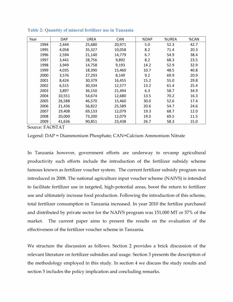
Table 2: Quantity of mineral fertilizer use in Tanzania
Year DAP UREA CAN %DAP %UREA %CAN 1994 2,444 25,680 20,971 5.0 52.3 42.7 1995 4,058 35,327 10,058 8.2 71.4 20.3 1996 2,594 21,140 14,779 6.7 54.9 38.4 1997 3,441 28,756 9,892 8.2 68.3 23.5 1998 3,949 14,758 9,193 14.2 52.9 32.9 1999 4,035 18,390 15,460 10.7 48.5 40.8 2000 3,576 27,293 8,149 9.2 69.9 20.9 2001 8,424 30,379 16,455 15.2 55.0 29.8 2002 6,515 30,334 12,577 13.2 61.4 25.4 2003 3,897 36,150 21,494 6.3 58.7 34.9 2004 10,551 54,674 12,680 13.5 70.2 16.3 2005 26,588 46,570 15,460 30.0 52.6 17.4 2006 21,436 56,822 25,589 20.6 54.7 24.6 2007 19,408 69,133 12,079 19.3 68.7 12.0 2008 20,000 73,200 12,079 19.0 69.5 11.5 2009 41,636 90,851 23,438 26.7 58.3 15.0
Source: FAOSTAT
Legend: DAP = Diammonium Phosphate; CAN=Calcium Ammonium Nitrate
In Tanzania however, government efforts are underway to revamp agricultural
productivity such efforts include the introduction of the fertilizer subsidy scheme
famous known as fertilizer voucher system. The current fertilizer subsidy program was
introduced in 2008. The national agriculture input voucher scheme (NAIVS) is intended
to facilitate fertilizer use in targeted, high-potential areas, boost the return to fertilizer
use and ultimately increase food production. Following the introduction of this scheme,
total fertilizer consumption in Tanzania increased. In year 2010 the fertilize purchased
and distributed by private sector for the NAIVS program was 151,000 MT or 57% of the
market. The current paper aims to present the results on the evaluation of the
effectiveness of the fertilizer voucher scheme in Tanzania.
We structure the discussion as follows. Section 2 provides a brick discussion of the
relevant literature on fertilizer subsidies and usage. Section 3 presents the description of
the methodology employed in this study. In section 4 we discuss the study results and
section 5 includes the policy implication and concluding remarks.
2. Literature review
Crop production in Tanzania and many SSA countries is faced with low use of fertilizer
and consequently low crop productivity. Several factors have been pointed out as cause
of low fertilizer use in SSA and Tanzania in particular. One of the factors is the high
uncertainty of water availability due to temporal rainfall variability, especially in rain-
fed agriculture (Van der Zaag, 2010). Water uncertainty inhibits poor farmers to invest
in the soil, and especially in fertilizer―a bad rainy season will lead to crop loss and thus
of the money invested. This is a risk that poor farming households cannot simply afford
to take. Another factor that is associated with the low use of fertilizer is the crop yield
response. It has been pointed out that the crop yield response to fertilizer use in Africa
has been much lower than in Asia, and that for many farmers fertilizer use may even
be uneconomic, especially those whose farms have poor soils (Kelly, 2005).
The problem of low fertilizer use in Africa is not a recent phenomenon and there has
been series of efforts to address the problem. however, the link between fertilizer policy
and fertilizer use in Africa is not very direct. During the 1960s and 1970s, fertilizer use
grew as rapidly in Africa as in other developing regions. According to the Food and
Agriculture Organization of the United Nations (FAO), annual growth in fertilizer use
in Sub-Saharan Africa was 9 percent over the 1960s and 1970s, but since 1981 fertilizer
use has stagnated at around 1.9–2.2 million metric tons (Morris et al., 2007; Bernson and
Minot, 2009).
During the 1970s and early 1980s, fertilizer programs in Africa were often characterized
by large, direct government expenditures using various entry points to stimulate
fertilizer demand and ensure supply. Interventions frequently included direct subsidies
that reduced fertilizer prices paid by farmers, government-financed and -managed
input credit programs, centralized control of fertilizer procurement and
distribution activities, and centralized control of key output markets (Morris et al.,
2007). However, Fertilizer promotion programs based on these types of interventions
generally did not lead to sustained growth in fertilizer use. Fertilizer subsidies remain
controversial. Many development economists and international development agencies
point to the high cost and limited effectiveness of fertilizer subsidies in the 1970s and
1980s (Benson, 2009).
It is pointed out that past subsidy programs, which often involved state monopolies in
fertilizer marketing, undermined the emergence of efficient, widespread, private input
distribution networks. It is argued that massive subsidization led to an inadequate
appreciation of fertilizer’s actual value and a complete neglect of issues like timeliness
and availability. For example during the period of heavy subsidies in many African
countries (mid-1980s), growth in fertilizer consumption was not particularly rapid.
Daramola (1989) concludes that chaotic and untimely fertilizer supply was one of the
most important reasons for non-adoption. Moreover, the rapid growth in fertilizer
consumption in the 1970s appeared to have slowed considerably in the last decade or
more. Nwosu (1995) argued that continuing the fertilizer subsidy cannot be justified on
grounds of efficiency or equity. Furthermore, there were significant opportunity costs to
devoting public funds to subsidizing fertilizer rather than investing in market
development, agricultural research, transportation infrastructure, or other public goods
to achieve a country’s development goals (Benson, 2009).
Another major concern with input subsides was the extent of leakages and diversion of
subsidized inputs away from their intended use. Farmers are likely to apply inputs to
the use from which they expect to get the greatest return. Fertilizers, for example, may
be applied to a variety of crops. If returns to fertilizers are higher on other crops (for
example cash crops) then farmers may apply subsidized fertilizers to cash crops which
have much more price elastic demand and which are not consumed by the poor
(Dorward, 2009).
It is pointed out that in general, where a general subsidy is applied it is difficult to
channel subsidized inputs to smallholder farmers. In such as case, a limited number of
tightly controlled supply chains, clear ways of identifying intended beneficiaries, and a
high degree of discipline and control of private fertilizer transactions are crucial
(Dorward, 2009).
If subsidized inputs are used by larger scale commercial farms this is likely to lead to
increased diversion away from staple food crop production to cash crops and a greater
share of transfers to less poor producers. Similar issues arise in subsidy access between
richer and poorer smallholders.
More recently, some policy makers have started to reconsider the prevailing thinking
about promoting fertilizer. In this case the interest is in large scale input subsidies, and
particularly fertilizer subsidies, in agricultural development and food security policies
(Dorward, 2009).
The main factors influencing large scale input subsidies include high global grain prices
in the first part of 2008 and the dramatic rises in fertilizer prices. Central point towards
fevering the subsidies in agricultural development mainly focuses on the need to
promote increased agricultural productivity through the adoption of up to date
technologies.
The concerned by the continuing low use of fertilizer by poor rural households,
including many whose members suffer from food insecurity, some have revived
arguments that the role of the state should be expanded to include not only commercial
marketing of fertilizer but also targeted distribution of subsidized fertilizer to poor
households that lack the resources needed to purchase fertilizer on a commercial
basis. The calls to reengage the public sector in fertilizer marketing and especially the
arguments supporting the use of fertilizer subsidies to provide a safety net for the poor
have sparked a lively policy debate that shows little sign of abating (Morris, et., 2007).
Jeffrey Sachs advocates large-scale distribution of low-cost or no-cost fertilizer as a way
of helping smallholders escape the so-called poverty trap. Sachs’s arguments have
struck a chord with some African political leaders, as evidenced during the Africa
Fertilizer Summit held in Abuja, Nigeria, in June 2006, where the case in favour of
fertilizer subsidies was argued by a number of participants.
Thus the assessment and evaluation on the effectiveness of the fertilizer subsidy
schemes is necessary. This is to devise an alternative means to ensure the intended goals
are achieved and that the past bad experience with the subsidy are not repeating. The
current paper is therefore pondering around this. What follows is the description of the
methodology employed to ascertain how well is the NAIVS is functioning in Tanzania
in terms of increasing crop productivity by the poor smallholders.
3. Methodology
Theoretical framework and modelling
The analytical framework used in this paper is the integration of modeling components
that range from the processes that are driven by the household economics to those that
are essentially biological in nature. Thus the methodology for this study is based on the
combination of the socioeconomic information obtained from the field survey and the
environmental information relevant in influencing crop production obtained from the
secondary sources. Our main consideration is to have the model that aim to take into
account the effect of voucher system in crop production since its establishment in 2008
to year 2012. Our thinking is that crop harvest by households in the study area is
affected by the household characteristic (socioeconomic and demographic), government
policy – fertilizer subsidy scheme and the environmental characteristics such as
weather, soil properties, topography etc. Therefore, the general model to include both
the socioeconomic and biophysical characteristic is appropriate in analyzing the effect
of fertilizer subsidy on crop production in the study area. In this case, households that
receive voucher and those who did not receive the fertilizer through voucher systems
were analyzed to gauge the differences in production that could be attributed by the
voucher program.
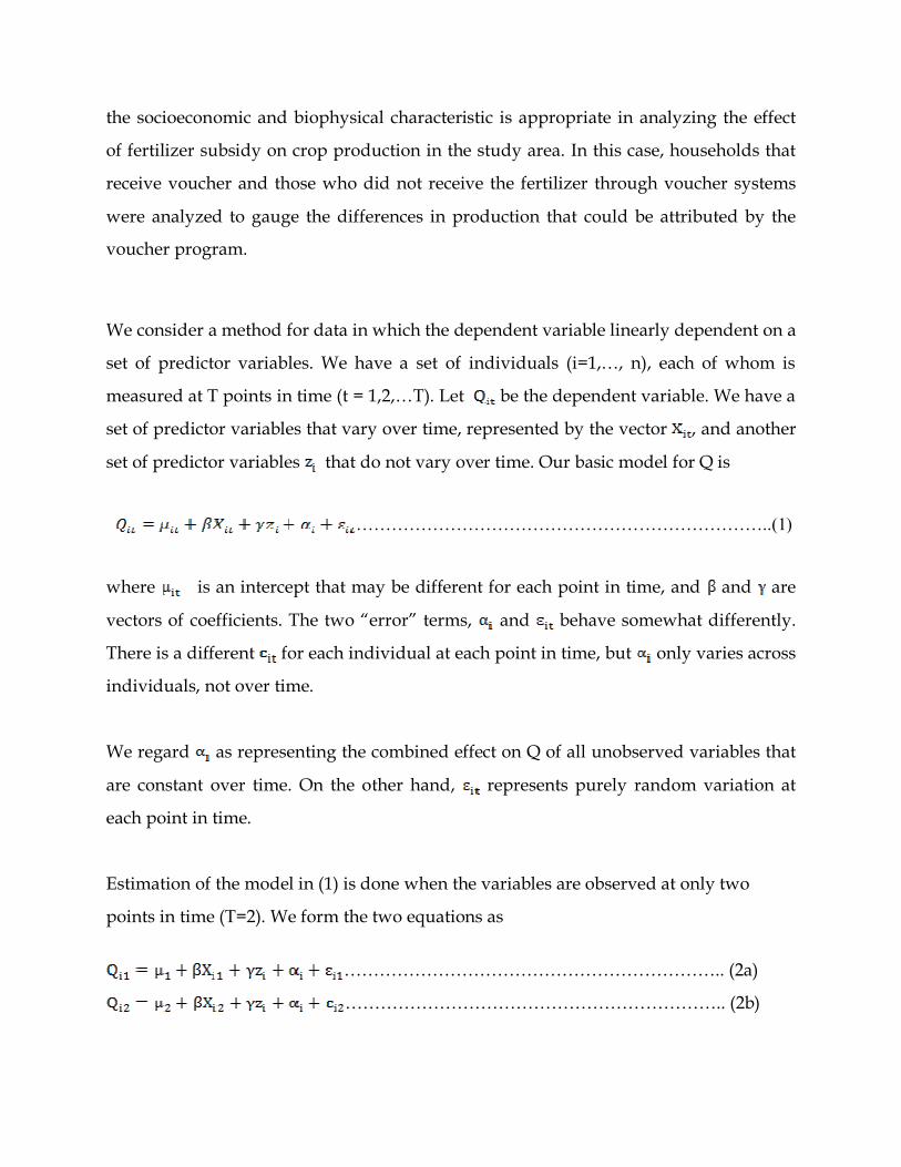
We consider a method for data in which the dependent variable linearly dependent on a
set of predictor variables. We have a set of individuals (i=1,…, n), each of whom is
measured at T points in time (t = 1,2,…T). Let be the dependent variable. We have a
set of predictor variables that vary over time, represented by the vector , and another
set of predictor variables that do not vary over time. Our basic model for Q is
……………………………………………………………..(1)
where is an intercept that may be different for each point in time, and and are
vectors of coefficients. The two “error” terms, and behave somewhat differently.
There is a different for each individual at each point in time, but only varies across
individuals, not over time.
We regard as representing the combined effect on Q of all unobserved variables that
are constant over time. On the other hand, represents purely random variation at
each point in time.
Estimation of the model in (1) is done when the variables are observed at only two
points in time (T=2). We form the two equations as
……………………………………………………….. (2a)
……………………………………………………….. (2b)

We form the first difference equation by subtracting 2a and 2b as shown in equation 3
)…………………………………………(3)
And finally we write an estimated model 4 as
……………………………………………………………………. (4).
We obtain consistent estimate of by regressing on .
Fixed effect Model (FEM) specification
Voucher system was introduced in the country in 2007 thus in order to effectively gauge
the impact of the scheme on crop production, the study employed the panel data
analysis technique.
One way to take into account the “individuality” of each farmer to let the intercept
vary for each farmer. The assumed variables to influence crop production in equation
1 exhibit different properties when time aspect is included in the analysis. Some
variables are time variant and others are time invariant. In this analysis, we run both
fixed and random effect and then test for the Hausman to gauge for the suitable model.
In order to run the fixed effect model, the study employs the Least Square Dummy
Variable (LSDV) approach. What follows is the description of the procedures to specify
the LSDV. At first the FEM is specified to include the quantity of harvest as dependent
variable and the independent variables are the farm size, quantity of fertilizer used,
household size, age of the head of household, household income.
………………………..….. (5)
Where
=quantity harvested (kg/acre), = farm size (acre), =quantity of fertilizer (kg),
=household size (number), =age of the head of the household (number), =

education level, =marital status, =main occupation, , =household
location, =cost of fertilizer, Sex of the head, =represent tth time period.
Secondly, a dummy variable to represent household receiving and those not receiving
fertilizers through voucher system is included in our modeling work. The included
dummy variable represents the effect of the voucher scheme on crop production at the
household level in the study area.
………………………………………………………………… (6)
Where =1 if the observation belongs to households with voucher, 0 otherwise. In
this model, in equation (5) is now represented by , represents the
intercept of household with voucher and represents the differential intercept
coefficient, which tell by how much the intercept of household with voucher differ
from the intercept of without voucher. Here Households without voucher becomes the
reference category.
Thirdly, we introduce the dummy variable to capture the effect of time passage on the
dependent variable. Just as we used the dummy variable to account for individual
(voucher) effect, we can allow for time effect because of factors such as technological
changes, changes in government regulatory and external effects such as weather. Such
time effects are accounted for by introducing time dummies. Since we have two years
we introduce one dummy as indicated in equation 7.
…………….….. (7)
Where takes a value of 1 for observation in year 2012 and 0 otherwise. We are
treating the year 2007 as the base year, whose intercept value is given by c1.

Finally we obtain the full fixed effect model in the LSDV approach. This is achieved by
combining model (6) and (7) with individual characteristics and time effects
respectively and form one model represented in equation 8.
………. (8)
By introducing the dummy variable the fixed effect model is now analyzed by the Least
Square Dummy Variable (LSDV) approach. The fixed-effects model controls for all
time-invariant differences between the individuals, so the estimated coefficients of the
fixed-effects models cannot be biased because of omitted time-invariant characteristics.
like culture, religion, gender, race, etc]. However, one side effect of the features of fixed-
effects models is that they cannot be used to investigate time-invariant causes of the
dependent variables. Technically, time-invariant characteristics of the individuals are
perfectly collinear with the person [or entity] dummies. Substantively, fixed-effects
models are designed to study the causes of changes within a person [or entity] Kohler,
Ulrich, Frauke Kreuter, Data Analysis Using Stata, 2nd ed., p.245. A time-invariant
characteristic cannot cause such a change, because it is constant for each person.
Random effect model (REM) specification
In this paper we also argue that the variation across households is assumed to be
random and uncorrelated with the predictor variables included in the model. We
believe that differences across households have some influence on the dependent
(quantity of harvest) and thus the need for random effect model. An advantage of
random effects is that we can include time invariant variables (i.e. gender)††. What
follows is the specification of the REM for this study. In the random effect model,
instead of treating as fixed as done in equation 5 above, we assume it is random
variable with mean . Furthermore, instead of using dummy variable to capture access
to voucher system, we use the error term, . Thus the REM is
†† In the fixed effects model these variables are absorbed by the intercept
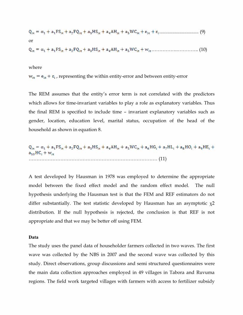
................................. (9)
or
…………….………….. (10)
where
, representing the within entity-error and between entity-error
The REM assumes that the entity’s error term is not correlated with the predictors
which allows for time-invariant variables to play a role as explanatory variables. Thus
the final REM is specified to include time – invariant explanatory variables such as
gender, location, education level, marital status, occupation of the head of the
household as shown in equation 8.
……………………………………………………………………… (11)
A test developed by Hausman in 1978 was employed to determine the appropriate
model between the fixed effect model and the random effect model. The null
hypothesis underlying the Hausman test is that the FEM and REF estimators do not
differ substantially. The test statistic developed by Hausman has an asymptotic χ2
distribution. If the null hypothesis is rejected, the conclusion is that REF is not
appropriate and that we may be better off using FEM.
Data
The study uses the panel data of householder farmers collected in two waves. The first
wave was collected by the NBS in 2007 and the second wave was collected by this
study. Direct observations, group discussions and semi structured questionnaires were
the main data collection approaches employed in 49 villages in Tabora and Ruvuma
regions. The field work targeted villages with farmers with access to fertilizer subsidy

through the agricultural inputs voucher system (AIVS) in two regions. Individual
household interviews were conducted on 327 smallholder farmers’ households across
the 49 villages within wards and districts of the selected regions. The information
gathered during the year 2012 was matched with the same households that were
surveyed in 2007 by the NBS. The 2012 survey was conducted to collect both qualitative
and quantitative data to analyze the impact of the Fertilizer subsidy on cereal crops
production and environment conservation. The sampling strategy for the 2012 survey
was that, purposive sampling technique was employed to select regions, districts,
wards, villages and households. The 2007 Census survey provided the sampling frame
that was used in 2012 survey. That is the household to be included in the 2012 survey
was one that was covered by the 2007 census survey. According 2007 census, 15
households were sampled in each village thus in the same way, the 2012 survey
purposively sample the same villages and same households. The field work took place
between March 2012 and April 2012. The research team composed of three principal
researchers and five research assistants. Generally, the field work was challenging in
terms of logistics to access the sampled households that were interviewed during 2007
census survey. With good cooperation received from village government we managed
to access and interview same households that were sampled in 2007/08 by the NBS
agriculture census survey. The survey targeted to interview the head or representative
of households. In addition, the study consulted and conducted the focus group
discussion with other stakeholders at all levels‡‡ to gain more understanding about
procedures and systems in general that governs the voucher scheme in the country. As
it is common practice in rural areas, majority of household do not keep records and
therefore the information/data collected from them depended much on their memory
recall.
In this paper, the maize crop was used as reference crop to analyze the impact of the
voucher system on crop production. The choice of this crop was due to two main ‡‡ Village, ward, district, region and ministry level

reason; (i) the voucher system includes two cereal crops maize and paddy (ii) most
households cultivate maize and paddy for both food and commercial purposes. In both
surveys small proportion of households cultivated paddy and thus were not used in the
analysis.
Construction of the panel data
The panel data analysis was based on the 654 observations consisting 327 households
from the first wave and second wave respectively. Before the analysis, the study first
made an attempt to match households and the respective information for the two
periods of interests. There after the merging of the two datasets was done in STATA.
This identification was created based on the codes created by the NBS for the location
(region, district, ward and village) and the household number that a household was
given during the 2007 survey.
5. Results
Descriptive statistics
The descriptive analysis of the variables from both survey data (Table 1) were used in
the panel data analysis. The rest of the variables are also available in Annex1. The
average quantity of maize harvested was 1,526.5 kg and 3,806 kg during 2007 and 2012
survey periods respectively.
The crop production in 2007 (during the time before the introduction of the voucher
system) found to differ significant with the crop production in 2012 (during the voucher
system). The F-test rejected the null hypothesis of no difference (F=23.49, Sig. 0.000)
between the mean maize harvest in 2007 and 2012. The average farm size was 2.3 acre
and 3.6 acre during the year 2007 and 2012 respectively. The difference between farm
size in 2007 and 2012 found to be statistically significant as confirmed by the F-test

(F=33.3, sig. 0.000). There was an increase in both the average area cultivated and the
quantity of harvests by households in 2007 and 2012. The major inputs used were
inorganic fertilizer, labour (family and hired labour) and seeds. The average cost of
inorganic fertilizer incurred by households farmers were Tsh 108,000 and 268,400
during 2007 and 2012 respectively. On average, household expenditure on farm inputs
were higher during 2012 than average costs incurred in 2007. This is a reflection of the
changes in the cost of production due to inflation. Most of the demographic
characteristics are time invariant as such the household head marital status and gender
are similar for both surveys. This is an indication that during the period of five years,
the households’ heads composition did not change. On the other hand, the average age
of the head of the household have increased from 47 to 50 years (Table3).
Table 3: Descriptive statistics for wave1 and wave 2 datasets
Variable
WAVE1 _ 2007 WAVE2 _ 2012 Obs1 Mean
Std. Dev. Min Max
Obs2 Mean
Std. Dev. Min Max
Maizeq 324 1526.5 1942.5 24.0 24000 324 3806.2 8240.2 34.0 66000.0 fsize 327 2.3 2.3 0.2 28.5 327 3.6 3.4 0.5 40.0 qty_fert 207 1234.5 7248.3 2.0 95000 278 265.4 586 16.0 6400.0 cost_fertilizer 205 108544 113175 60.0 98000 235 268476 329953 3200 1800000
cost_seeds 326 14176 21991 150 20000
0 157 41848 51962.0 10000 299000.0 o_farmer 327 0.9 0.3 0 1 327 0.9 0.3 0 1 edn_none 327 0.1 0.3 0 1 327 0.1 0.3 0 1 edn_pr 327 0.9 0.3 0 1 327 0.9 0.3 0 1 edn_sec 327 0.1 0.2 0 1 327 0.1 0.2 0 1 edn_tert 327 0.0 0.1 0 1 327 0.0 0.1 0 1 sex 327 0.9 0.4 0 1 327 0.9 0.4 0 1 marital 327 0.8 0.4 0 1 327 0.8 0.4 0 1 Age 327 47.0 14.7 20.0 89.0 327 49.7 14.2 19 95
Legend: Maizeq= quantity of maize harvested (kg); fsize=farm size cultivated (acre); qty_fert=quantity of inorganic fertilizer used (kg); cost_fert= cost of inorganic fertilizer incurred (Tshs); cost_seed=cost of improved seeds (Tshs); o_farmer=farming as main occupation (binary 1 or 0); edc_none=not gone to school (binary 0 or 1); edn_pr=primary level of education with schooling years 1 to 8 (binary 1 or 0), edn_sec= secondary school level of education (binary (0
or 1); edn_tert=tertiary level of education (binary 1 or 0); sex= sex of the head of the household; marital=marital status of the head binary 1 or 0); age= age of the head of household
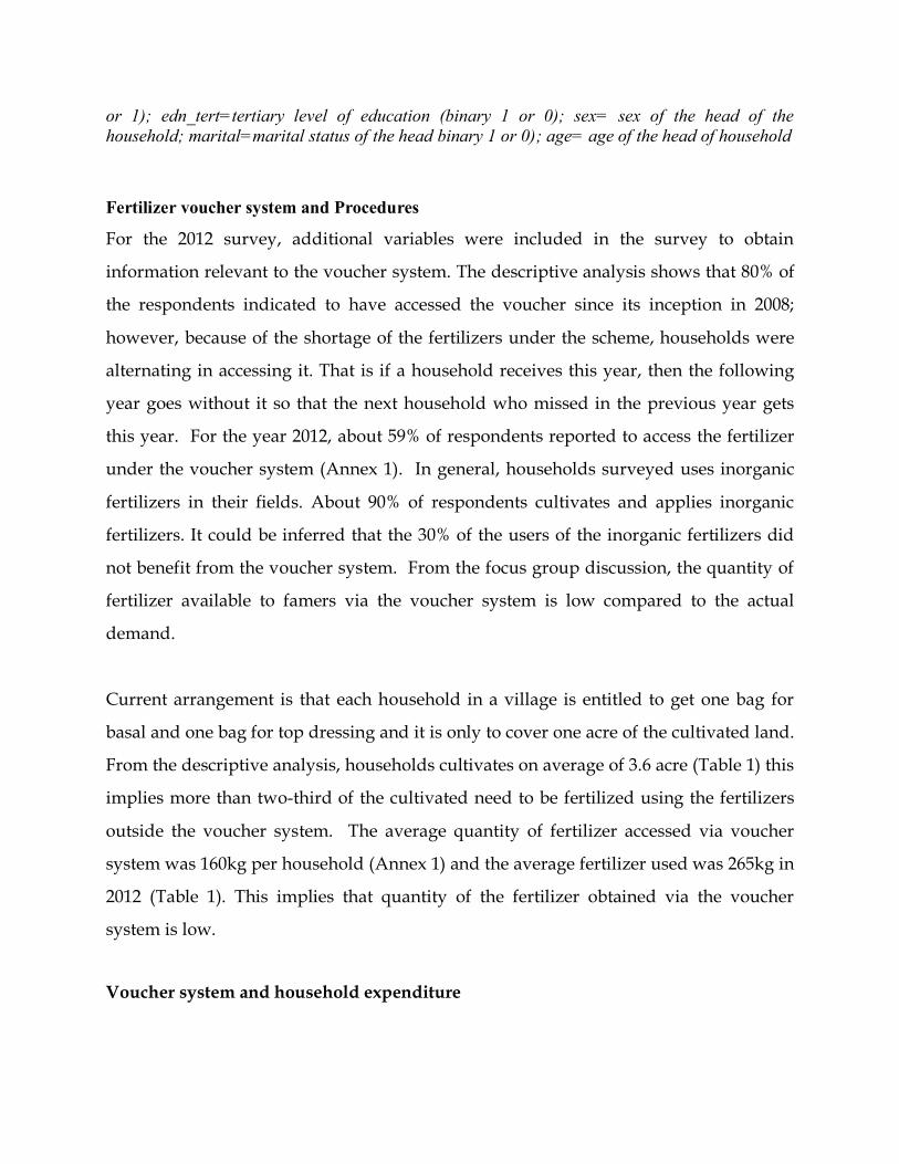
Fertilizer voucher system and Procedures
For the 2012 survey, additional variables were included in the survey to obtain
information relevant to the voucher system. The descriptive analysis shows that 80% of
the respondents indicated to have accessed the voucher since its inception in 2008;
however, because of the shortage of the fertilizers under the scheme, households were
alternating in accessing it. That is if a household receives this year, then the following
year goes without it so that the next household who missed in the previous year gets
this year. For the year 2012, about 59% of respondents reported to access the fertilizer
under the voucher system (Annex 1). In general, households surveyed uses inorganic
fertilizers in their fields. About 90% of respondents cultivates and applies inorganic
fertilizers. It could be inferred that the 30% of the users of the inorganic fertilizers did
not benefit from the voucher system. From the focus group discussion, the quantity of
fertilizer available to famers via the voucher system is low compared to the actual
demand.
Current arrangement is that each household in a village is entitled to get one bag for
basal and one bag for top dressing and it is only to cover one acre of the cultivated land.
From the descriptive analysis, households cultivates on average of 3.6 acre (Table 1) this
implies more than two-third of the cultivated need to be fertilized using the fertilizers
outside the voucher system. The average quantity of fertilizer accessed via voucher
system was 160kg per household (Annex 1) and the average fertilizer used was 265kg in
2012 (Table 1). This implies that quantity of the fertilizer obtained via the voucher
system is low.
Voucher system and household expenditure
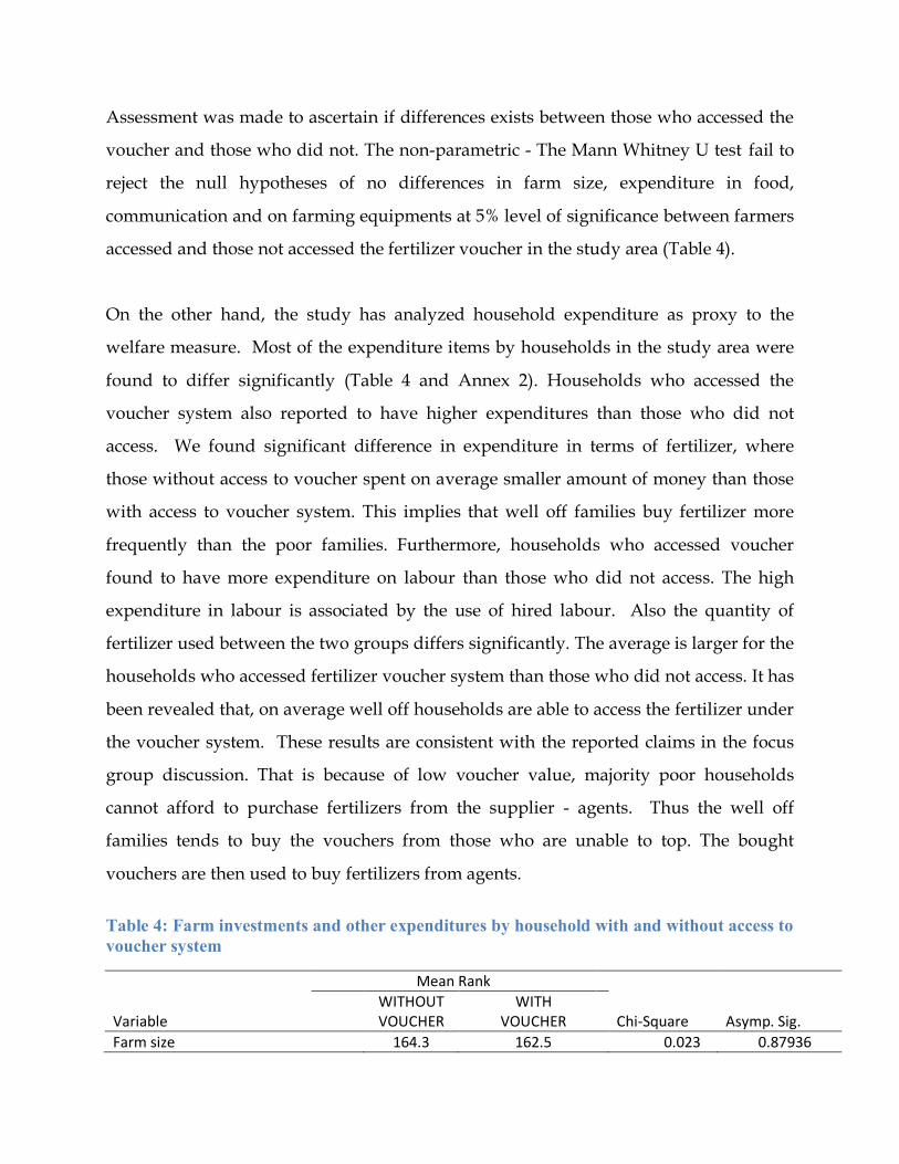
Assessment was made to ascertain if differences exists between those who accessed the
voucher and those who did not. The non-parametric - The Mann Whitney U test fail to
reject the null hypotheses of no differences in farm size, expenditure in food,
communication and on farming equipments at 5% level of significance between farmers
accessed and those not accessed the fertilizer voucher in the study area (Table 4).
On the other hand, the study has analyzed household expenditure as proxy to the
welfare measure. Most of the expenditure items by households in the study area were
found to differ significantly (Table 4 and Annex 2). Households who accessed the
voucher system also reported to have higher expenditures than those who did not
access. We found significant difference in expenditure in terms of fertilizer, where
those without access to voucher spent on average smaller amount of money than those
with access to voucher system. This implies that well off families buy fertilizer more
frequently than the poor families. Furthermore, households who accessed voucher
found to have more expenditure on labour than those who did not access. The high
expenditure in labour is associated by the use of hired labour. Also the quantity of
fertilizer used between the two groups differs significantly. The average is larger for the
households who accessed fertilizer voucher system than those who did not access. It has
been revealed that, on average well off households are able to access the fertilizer under
the voucher system. These results are consistent with the reported claims in the focus
group discussion. That is because of low voucher value, majority poor households
cannot afford to purchase fertilizers from the supplier - agents. Thus the well off
families tends to buy the vouchers from those who are unable to top. The bought
vouchers are then used to buy fertilizers from agents.
Table 4: Farm investments and other expenditures by household with and without access to voucher system
Mean Rank
Variable
WITHOUT VOUCHER
WITH VOUCHER Chi-Square Asymp. Sig.
Farm size 164.3 162.5 0.023 0.87936

Maize harvest 120.5 177.7 23.555 0.00000 Expenditure on labour 135.8 174.2 13.662 0.00022 Expenditure on seeds 113.5 182.3 39.338 0.00000 Expenditure on food 136.3 132.6 0.113 0.73625 Expenditure on communication 102.6 119.1 2.422 0.11963 Expenditure on medical 136.1 158.2 3.674 0.05527 Expenditure on education 106.4 144.9 12.204 0.00048 Expenditure on Transport 100.0 125.7 5.724 0.01674 Expenditure on farm equipments 98.6 97.2 0.018 0.89197 Expenditure on inorganic fertilizer 112.1 182.8 36.477 0.00000 Quantity of inorganic fertilizers 102.9 146.9 12.010 0.00053
Source: Estimation by authors Panel data analysis results
The panel data analysis employed to establish factors influencing crop production using
the fixed and random effete models. However, following the results obtained after the
Hausman test, the random effect model found to be the appropriate and thus was used
to estimate model parameters and variable coefficients (Table 5). The result from the
panel analysis shows that maize crop during the period 2007 and 2012 has been
influenced by farm size, quantity of inorganic fertilizer, expenditure on the inorganic
fertilizer, access to the voucher system, expenditure on improved seed and location
specific factors. The demographic factors influencing significantly the maize production
was only head of the household. Others such as household size, marital status, sex of
the head of the head of the household found to be insignificant (Table 5). The use of
improved seeds has resulted to an increase in crop production in the study area. The
increased of use of improved seeds by 10% results to an increase in maize harvest by
0.8% holding other factors. An increase purchase of inorganic fertilizers by 10% would
result to an increase of maize harvest by 13% of maize harvest. In addition, the increase
in farm size by 10% results to an increase in maize harvest by 12%. The location
specific factors were found to influence maize production in the study area (Table 5).
Table 5 : Factors influencing maize crop production in the study area
Variable Description RE model
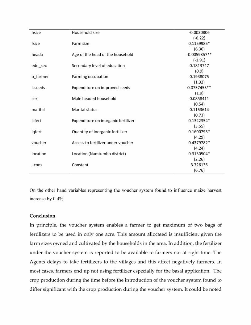
hsize Household size -0.0030806 (-0.22)
fsize Farm size 0.1159985* (6.36)
heada Age of the head of the household -0.0059357** (-1.91)
edn_sec Secondary level of education 0.1813747 (0.9)
o_farmer Farming occupation 0.1938075 (1.32)
lcseeds Expenditure on improved seeds 0.0757453** (1.9)
sex Male headed household 0.0858411 (0.54)
marital Marital status 0.1153614 (0.73)
lcfert Expenditure on inorganic fertilizer 0.1322354* (3.55)
lqfert Quantity of inorganic fertilizer 0.1600793* (4.29)
voucher Access to fertilizer under voucher 0.4379782* (4.24)
location Location (Namtumbo district) 0.3130504* (2.26)
_cons Constant 3.726135 (6.76)
On the other hand variables representing the voucher system found to influence maize harvest
increase by 0.4%.
Conclusion
In principle, the voucher system enables a farmer to get maximum of two bags of
fertilizers to be used in only one acre. This amount allocated is insufficient given the
farm sizes owned and cultivated by the households in the area. In addition, the fertilizer
under the voucher system is reported to be available to farmers not at right time. The
Agents delays to take fertilizers to the villages and this affect negatively farmers. In
most cases, farmers end up not using fertilizer especially for the basal application. The
crop production during the time before the introduction of the voucher system found to
differ significant with the crop production during the voucher system. It could be noted
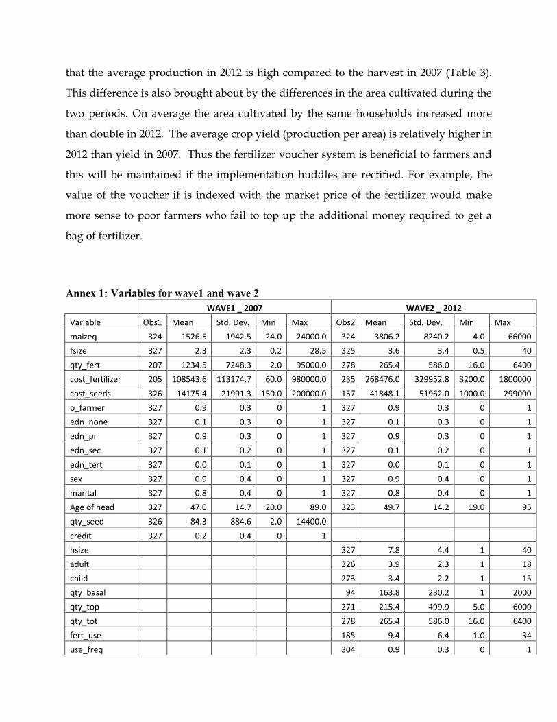
that the average production in 2012 is high compared to the harvest in 2007 (Table 3).
This difference is also brought about by the differences in the area cultivated during the
two periods. On average the area cultivated by the same households increased more
than double in 2012. The average crop yield (production per area) is relatively higher in
2012 than yield in 2007. Thus the fertilizer voucher system is beneficial to farmers and
this will be maintained if the implementation huddles are rectified. For example, the
value of the voucher if is indexed with the market price of the fertilizer would make
more sense to poor farmers who fail to top up the additional money required to get a
bag of fertilizer.
Annex 1: Variables for wave1 and wave 2
WAVE1 _ 2007 WAVE2 _ 2012
Variable Obs1 Mean Std. Dev. Min Max Obs2 Mean Std. Dev. Min Max maizeq 324 1526.5 1942.5 24.0 24000.0 324 3806.2 8240.2 4.0 66000 fsize 327 2.3 2.3 0.2 28.5 325 3.6 3.4 0.5 40 qty_fert 207 1234.5 7248.3 2.0 95000.0 278 265.4 586.0 16.0 6400 cost_fertilizer 205 108543.6 113174.7 60.0 980000.0 235 268476.0 329952.8 3200.0 1800000 cost_seeds 326 14175.4 21991.3 150.0 200000.0 157 41848.1 51962.0 1000.0 299000 o_farmer 327 0.9 0.3 0 1 327 0.9 0.3 0 1 edn_none 327 0.1 0.3 0 1 327 0.1 0.3 0 1 edn_pr 327 0.9 0.3 0 1 327 0.9 0.3 0 1 edn_sec 327 0.1 0.2 0 1 327 0.1 0.2 0 1 edn_tert 327 0.0 0.1 0 1 327 0.0 0.1 0 1 sex 327 0.9 0.4 0 1 327 0.9 0.4 0 1 marital 327 0.8 0.4 0 1 327 0.8 0.4 0 1 Age of head 327 47.0 14.7 20.0 89.0 323 49.7 14.2 19.0 95 qty_seed 326 84.3 884.6 2.0 14400.0 credit 327 0.2 0.4 0 1 hsize 327 7.8 4.4 1 40 adult 326 3.9 2.3 1 18 child 273 3.4 2.2 1 15 qty_basal 94 163.8 230.2 1 2000 qty_top 271 215.4 499.9 5.0 6000 qty_tot 278 265.4 586.0 16.0 6400 fert_use 185 9.4 6.4 1.0 34 use_freq 304 0.9 0.3 0 1
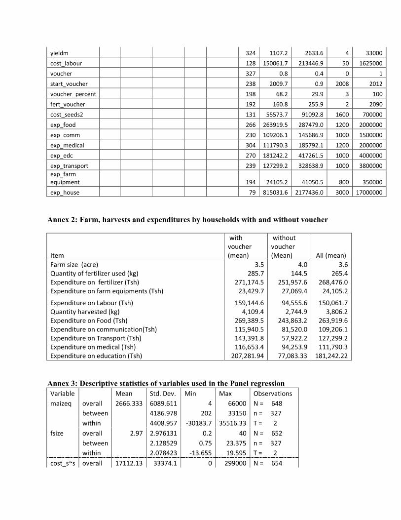
yieldm 324 1107.2 2633.6 4 33000 cost_labour 128 150061.7 213446.9 50 1625000 voucher 327 0.8 0.4 0 1 start_voucher 238 2009.7 0.9 2008 2012 voucher_percent 198 68.2 29.9 3 100 fert_voucher 192 160.8 255.9 2 2090 cost_seeds2 131 55573.7 91092.8 1600 700000 exp_food 266 263919.5 287479.0 1200 2000000 exp_comm 230 109206.1 145686.9 1000 1500000 exp_medical 304 111790.3 185792.1 1200 2000000 exp_edc 270 181242.2 417261.5 1000 4000000 exp_transport 239 127299.2 328638.9 1000 3800000 exp_farm equipment 194 24105.2 41050.5 800 350000 exp_house 79 815031.6 2177436.0 3000 17000000
Annex 2: Farm, harvests and expenditures by households with and without voucher
Item
with voucher (mean)
without voucher (Mean) All (mean)
Farm size (acre) 3.5 4.0 3.6 Quantity of fertilizer used (kg) 285.7 144.5 265.4 Expenditure on fertilizer (Tsh) 271,174.5 251,957.6 268,476.0 Expenditure on farm equipments (Tsh) 23,429.7 27,069.4 24,105.2
Expenditure on Labour (Tsh) 159,144.6 94,555.6 150,061.7 Quantity harvested (kg) 4,109.4 2,744.9 3,806.2 Expenditure on Food (Tsh) 269,389.5 243,863.2 263,919.6 Expenditure on communication(Tsh) 115,940.5 81,520.0 109,206.1 Expenditure on Transport (Tsh) 143,391.8 57,922.2 127,299.2 Expenditure on medical (Tsh) 116,653.4 94,253.9 111,790.3 Expenditure on education (Tsh) 207,281.94 77,083.33 181,242.22
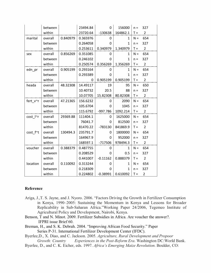
Annex 3: Descriptive statistics of variables used in the Panel regression Variable
Mean Std. Dev. Min Max Observations
maizeq overall 2666.333 6089.611 4 66000 N = 648
between
4186.978 202 33150 n = 327
within
4408.957 -30183.7 35516.33 T = 2
fsize overall 2.97 2.976131 0.2 40 N = 652
between
2.128529 0.75 23.375 n = 327
within
2.078423 -13.655 19.595 T = 2
cost_s~s overall 17112.13 33374.1 0 299000 N = 654
between
23494.84 0 156000 n = 327
within
23720.64 -130638 164862.1 T = 2
marital overall 0.840979 0.365976 0 1 N = 654
between
0.264058 0 1 n = 327
within
0.253611 0.340979 1.340979 T = 2
sex overall 0.856269 0.351085 0 1 N = 654
between
0.246102 0 1 n = 327
within
0.250574 0.356269 1.356269 T = 2
edn_pr overall 0.905199 0.293164 0 1 N = 654
between
0.293389 0 1 n = 327
within
0 0.905199 0.905199 T = 2
heada overall 48.32308 14.49117 19 95 N = 650
between
10.40732 20.5 88 n = 327
within
10.07705 15.82308 80.82308 T = 2
fert_v~r overall 47.21365 156.6232 0 2090 N = 654
between
105.6704 0 1045 n = 327
within
115.6792 -997.786 1092.214 T = 2
cost_l~r overall 29369.88 111404.1 0 1625000 N = 654
between
76041.7 0 812500 n = 327
within
81470.22 -783130 841869.9 T = 2
cost_f~t overall 130494.3 235791.7 0 1800000 N = 654
between
164967.9 0 952000 n = 327
within
168597.1 -717506 978494.3 T = 2
voucher overall 0.388379 0.487755 0 1 N = 654
between
0.208529 0 0.5 n = 327
within
0.441007 -0.11162 0.888379 T = 2
location overall 0.110092 0.313244 0 1 N = 654
between
0.218309 0 1 n = 327
within
0.224802 -0.38991 0.610092 T = 2
Reference Ariga, J.,T. S. Jayne, and J. Nyoro. 2006. “Factors Driving the Growth in Fertilizer Consumption
in Kenya, 1990–2005: Sustaining the Momentum in Kenya and Lessons for Broader Replicability in Sub-Saharan Africa.”Working Paper 24/2006, Tegemeo Institute of Agricultural Policy and Development, Nairobi, Kenya.
Benson, T and N. Minot. 2009. Fertilizer Subsidies in Africa. Are voucher the answer?. IFPRI issue Brief 60.
Breman, H., and S. K. Debrah. 2004. “Improving African Food Security.” Paper Series P-31. International Fertilizer Development Center (IFDC).
Byerlee,D., X. Diao, and C. Jackson. 2005. Agriculture, Rural Development and Propoor Growth: Country Experiences in the Post-Reform Era. Washington DC:World Bank. Byerlee, D., and C. K. Eicher, eds. 1997. Africa’s Emerging Maize Revolution. Boulder, CO:
Lynne Rienner. Cleaver, K. M., and G. A. Schreiber. 1994. Reversing the Spiral: The Population, Agriculture, and Environment Nexus in Sub-Saharan Africa.Washington, DC:World Bank. Crawford, E. W., T. S. Jayne, and V. A. Kelly. 2006. “Alternative Approaches for Promoting
Fertilizer Use in Africa.” Agriculture and Rural Development Discussion Paper 22,World Bank,Washington, DC.
Debra, K. 2002. “Agricultural Subsidies in Sub-Saharan Africa: A Reflection.”PowerPoint presentation made at the Second Regional Meeting of Agro Inputs Trade Associations in West and Central Africa, Mercure Sarakawa Hotel, Lomé, Togo, December 5–6. IFDC Africa Division.
Dorward, A. 2009. Rethinking agricultural input subsidy programmes in a changing world. Paper prepared for the Trade and Markets Division, Food and Agriculture Organization of the United Nations.
FAOSTAT. Statistical database. http://faostat.fao.org/. FAO (Food and Agriculture Organization). 1986. African Agriculture: The Next 25 Years. Annex V, Inputs Supply and Incentive Policies. Rome: FAO FAO (Food and Agriculture Organization)2005. “Increasing Fertilizer Use and Farmer Access in
Sub-Saharan Africa: A Literature Review.” Agricultural Management, Marketing, and Finance Service (AGSF), Agricultural Support Systems Division, FAO, Rome.
Govereh, J., and T. Jayne. 2003. “Cash Cropping and Food Crop Productivity: Synergies or Trade-offs?” Agricultural Economics 28 (1): 39–50. Gregory, D. I., and B. L. Bumb. 2006. “Factors Affecting Supply of Fertilizer in Sub-Saharan
Africa.” Agriculture and Rural Development, Discussion Paper 24,World Bank,Washington, DC.
Gulati, A., and S. Narayanan. 2003. The Subsidy Syndrome in Indian Agriculture. New Delhi: Oxford University Press.
Jayne, T. S., G. J. and X. Zu. 2007. Fertilizer Promotion in Zambia: Implications for Strategies to Raise Smallholder Productivity. Seminar at World Bank, Washington DC: November. Kelly,V. A. 2006. “Factors Affecting Demand for Fertilizer in Sub-Saharan Africa.”
Agriculture and Rural Development Discussion Paper 23, World Bank, Washington, DC. Kelly,V. A., and M. L. Morris. 2006. “Promoting Fertilizer to Increase Productivity in African
Cereals Systems: What Role for Subsidies?” Paper prepared for the organized symposium, “Seed/Fertilizer Technology, Cereal Productivity, and Pro-Poor Growth in Africa:Time for New Thinking?” 26th Conference of the International Association of Agricultural Economists (IAAE), Gold Coast, Queensland, Australia, August 12–18.
Morris, M., V.A. Kelly, R.J. Kopicki and D. Byerlee. 2007. “Fertilizer Use in African Agriculture: Lesson Learned and Good Practice Guideline. Washington DC:World Bank. Morris, M., V. A. Kelly, R. Kopicki and D. Byerlee (2007). Fertilizer use in African agriculture.
Washington D.C., World Bank. Schultz, J. J., and D. H. Parish. 1989. “Fertilizer Production and Supply Constraints and Options in Sub-Saharan Africa.” Paper Series P-10, IFDC, Muscle Shoals, AL. URT (2010) National Sample Census of Agriculture 2007/08: Preliminary Report Wooldridge, J. M. (2001), Econometric Analysis of Cross Section and Panel Data, Cambridge, MA: MIT Press.


