The Transmission of Monetary Policy Within Banks:Evidence from India
Abhiman Das, Prachi Mishra, and N. R. Prabhala∗
April 7, 2016
Abstract
Over the last two decades, India’s central bank injected or drained liquidity from banksthrough changes in cash reserve requirements. We analyze the lending responses tothese quantitative tools of monetary policy using branch level lending data. We focuson frictions within banks that influence transmission, in contrast to prior work thatfocuses on external frictions between banks and funding markets, which we control forin a saturated specification with high order interactive bank-year and region-year fixedeffects. We show that the intra-bank variation in lending is economically significant.A rich set of branch level asset, liability, and organizational variables explain the intra-bank transmission. Branches that are larger, make loans with smaller ticket size, aredeposit rich, make shorter term loans, have fewer non non performing assets, and withgreater managerial capacity respond more to monetary policy. Transmission effects aremore sluggish in state-owned banks.
∗Abhiman Das is at the Indian institute of Management, Ahmedabad and can be reached at [email protected]. Prachi Mishra is at the IMF and Reserve Bank of India and can be reached [email protected]. Prabhala is at CAFRAL and University of Maryland, College Park and can bereached at [email protected]. We thank Viral Acharya, Sumit Agarwal, Saugata Bhattacharya, CharlesCalomiris, Anusha Chari, Goutam Chatterjee, Indranil Sengupta, Peter Montiel, Urjit Patel, Raghuram Ra-jan, Prasanna Tantri, Bernard Yeung, and seminar participants at the ISB CAF summer conference, NUSBusiness School, NYU Stern School of Business, Reserve Bank of India, Society for Economic Research inIndia, UC San Diego, UCLA, Indian Statistical Institute, NIPFP-DEA conference, and the NBER-ICRIERNeemrana conference, for many useful comments and suggestions. We thank Madhav Kumar for excellent re-search assistance. The views expressed are those of the authors and not of the institutions they are affiliatedwith. We retain responsibility for any remaining errors. Any remaining errors are ours alone.

1 Introduction
Central banks set monetary policy. How the policy is transmitted through the financial
system has been a question of long-standing interest to both policy makers and academics.
Understanding transmission has become especially important after the 2008 financial crisis.
Doubts and debates about the efficacy of fiscal policy, political debates surrounding its
size, scope, and form, plus inside and outside lags in its implementation, have combined to
give monetary policy a central role in macroeconomic stabilization. How banks respond to
monetary policies remains an important and relevant economic question.
We provide new evidence on bank responses to monetary stimulus using a dataset of
over a billion loan accounts between 1996 and 2013 in India. Our analysis is of interest from
three viewpoints. First, we characterize transmission within banks. We show that the within-
bank variation is economically important and characterize its nature using a rich dataset on
bank branch characteristics. The takeaway from the analysis is that besides the external
frictions between banks and markets emphasized (rightly) in prior work, internal or intra-
bank frictions also matter. A second point of interest is the tool of monetary policy. We focus
on essentially instantaneous injections or retractions of cash by the central bank into banks in
a formulaic fashion. Thus, we study a direct version of the widely discussed “helicopter drop
of money” into banks. Finally, we introduce granular controls for unobservable heterogeneity
through saturated bank-year and local geography-year interactive effects.
We contribute to the work on the bank lending channel of monetary transmission. As
Kashyap and Stein (1995) write, aggregate analyses of transmisson can be explained away
with “...a sufficiently creative story about heterogeneity in credit demand.”1 Thus, much
of the literature focuses on heterogeneity in responses across banks. A focal prediction
tested in this work is that banks facing external financing frictions are more responsive to
monetary policy (Kashyap and Stein (2000)). While the goal of this literature which utilized
cross-sectional variation was to firm up evidence of a bank lending channel, the basic tool
1From their article, “... almost any movement in the composition of external finance can be explainedaway by appealing to a sufficiently creative story about heterogeneity in credit demand.
1

of exploiting heterogeneity between banks is used in many other settings. For instance,
Campello (2002) uses it to analyze standalone banks versus those in conglomerates while
Khwaja and Mian (2008) and Cetorelli and Goldberg (2012) use it to understand global
transmission of monetary shocks. Peek and Rosengren (2013) provide a recent and relatively
thorough survey of the literature on monetary transmission.
Our contribution to this cross-sectional literature is to highlight that besides external
frictions between banks and markets, internal frictions within banks also matter. To begin
with, CRR changes alter the financial resources available to banks at headquarters level. How
they translate into micro-lending outcomes depends on the organizational hierarchies that
allocate capital internally (Stein (1997), Stein (2002)). As Cetorelli and Goldberg (2012) and
Skrastins and Vig (2014) remark, micro-level data on these aspects are scarce. We contribute
towards filling the gap. Consistent with this literature, we show that the variation in lending
within banks is economically important. The finding is sensible. Credit origination is driven
by branches while the sign-off authority can traverse many layers depending on the credit
size, complexity, and the type of organization, e.g., state-owned or private banks. We exploit
the data on branch characteristics to understand the nature of internal frictions that can
modulate the within-variation.
Our analysis is also of econometric interest. Our approach of studying within-bank
variation takes the cross-sectional approach a step further by soaking up a considerable
amount of unobserved heterogeneity. Bank-year interactive fixed effects absorb the across-
bank variation such as liquidity or capital shortages, even those that vary from year to year.
District-year fixed effects absorb local geographical variation in credit including the annual
fluctuations due to factors such as weather or economic activity. The branch level responses
thus rule out heterogeneity due to entity, geography, and its variation year to year.2
Another point of interest is the tool of monetary policy, the cash reserve ratio (CRR).
The ratio denotes the cash balances that banks operating in India must maintain with
its central bank. Increases in CRR drain funds from banks while decreases inject funds
2The district controls are granular. As of December 2015, India has 683 districts.
2

into banks. These injections or drainages of money take immediate effect so they free up
or retract loanable resources instantaneously. Moreover, the funding changes are specified
formulaically as a percentage of deposits without regard to any individual bank’s condition
and place no restrictions on the end-use of resources. These changes are frequent in both
directions during the sample period. They are also potent. Banks earn no interest on CRR
while lending rates are in or near double-digits during our sample period. If a bank fails
to maintain the minimum CRR, it must pay the RBI a penal interest rate with spreads
of between 300 to 500 basis points above bank lending rates. CRR changes are also of
current policy interest as they are deployed elsewhere. For instance, China cut its reserve
requirements on February 29, 2016 to ease credit conditions.
Our study of cash injections or drainages also informs an extensive literature on financ-
ing constraints. Much of the literature centers on non-financial firms.3. While the role of
constraints in non-financial firms is well understood, Kashyap and Stein (1995) and Kashyap
and Stein (2000) point out that exactly the same frictions can exist for financial firms such
as banks that have opaque assets. Our study contributes to the literature by developing
micro evidence on the effects of one type of intervention to relieve financial constraints.
Branches are important sources of both economic and econometric variation. Our sample
comprises 150 banks operating through 126,873 branches that are located in 653 adminis-
trative districts spread over 29 states and 7 union territories. Within-bank variation is
quantitatively important. A two-way variation decomposition across banks shows that the
within-variation dominates, and its share increases over time. For instance, it accounts for
73% at the beginning of our sample period and 90% of the variance in 2013. Even in the
same geographical location, the variation within banks is higher. Within bank or across
branch variation inside districts accounts for 86% of the variance in 1996 and 91% in 2013.
In practice, lending proposals originate at the branch. Line staff screen and conduct
credit analysis according to processes set or approved by headquarters. What happens next
3 See, e.g., Lamont (1997), Fazzari, Hubbard, and Petersen (1988), Kaplan and Zingales (1997), Whitedand Wu (2006), Hennessy and Whited (2007), Paravasini (2008), Hadlock and Pierce (2010), Ball, Hoberg,and Maksimovic (2015), Farre-Mensa and Ljungqvist (2016)
3

depends on the nature of the credit. Some credits can be locally approved while others move
up the bank hierarchy to either the region or national level. In our sample period, relatively
few businesses are handled through centralized verticals. Branches are increasingly delegated
authority for lending decisions for which expertise likely resides in branches.4Branches are
also institutionally relevant. India’s nationalization of its banking sector in 1969 created
a large state-owned bank network and a highly regulated banking sector with significant
entry barriers. Banks cannot open except through licensing, which are granted relatively
infrequently. Branches are, however, easier to open. They are also a key focus of regulators,
who require banks to reach out to the unbanked through branch networks (Burgess and
Pande (2005), Cole (2009)).
We adapt the Kashyap and Stein (2000) framework to branch level data. Credit at the
bank, branch, and the year level is the response variable. Our data come from the Reserve
Bank of India Basic Statistical Returns (BSR), which has over a billion individual loan
observations. We aggregate BSR data into 1.04 million bank-branch-year loan observations.
The dataset has identifiers for bank, amount, and the originating branch. We explain credit
using the monetary policy variable, CRR, plus controls. Our focus is on the interactions
between CRR and branch characteristics. We also include triple interaction effects, for
example, between CRR, branch characteristics and an indicator for whether the bank is
state-owned or private.
One category of variables represents the type of loan. Loan ticket size drives the delega-
tion of loan authority whether for approval or review. Small loans are handled at the branch
level while larger loans require zonal, regional, or headquarter level approval. Likewise,
long-term loans require greater investment in information gathering and analysis. Branches
dealing with these more complex types of credit are less likely to respond to monetary stimuli.
Larger branches are likely to be repositories of greater expertise and organizational capital
in lending. These branches are likely to house more senior managers with greater lending
4In one large bank we talked to in December 2015, a branch manager can automatically sign off on loansof up to |20 million, or about $300,000. Larger or complex loans require clearance from bank hierarchy. Seealso Skrastins and Vig (2014).
4

experience and are likely to have better processing capacity to handle loan flows. The
interactions and communications with headquarters are also likely to be more, so lending
frictions are likely lower in large branches.
Another characteristic likely to drive lending responses is the availability of local resources
at the branch. Whether deposit rich branches lend more in response to monetary injection
at the headquarters is an interesting question. Branches not rich in resources may be ready
targets for any new resources available at headquarters. However, if deposit gathering is
costly and headquarters readily funds deficits, branches may have less incentives to gather
deposits. In this situation, headquarters may allocate more resources to branches that raise
more internal deposits. Thus, lending responses can be greater for branches rich in deposits.
We also use a lag of the credit to deposit ratio as an explanatory variable. Consider a bank
with $1 of deposits. The extent to which the $1 is deployed in lending depends on the costs
of making loans, which includes the costs of finding customers, screening them, processing
the loans, and monitoring the loan ex-post. Banks lend to the point where revenues from
lending equal the marginal costs of finding, processing, and monitoring a new customer.
Banks with higher costs will lend less and have lower credit to deposit ratios. Of course,
credit to deposit ratios are also functions of local demand conditions, but the inclusion of
district-year interactive fixed effects controls for these conditions.
We also analyze differences between rural and urban areas. This dimension is of both
economic and practical interest. In India, rural branches are characterized by excess demand
for credit relative to supply. Given the excess credit demand in rural areas, the supply
side responses of banks to injections or withdrawal of loanable funds are more likely to be
reflected in greater credit expansion or contraction in rural branches relative to their urban
counterparts. These effects are likely to be more pronounced in state-owned banks that
have long histories of operation in rural areas. At the same time, rural areas are difficult
to reach, therefore rural loans may be difficult to make. A distance to lending story, on the
lines of Petersen and Rajan (2002), would imply that transmission should be weaker in rural
branches.
5

We next focus on branch level non-performing assets (NPAs). The risk-taking channel of
monetary transmission has attracted great interest. Loose monetary policy is often blamed
for the 2008 financial crisis as it pushed financial firms to seek higher yields (Rajan, 2005,
Diamond and Rajan, 2009). On the other hand, poor loan performance can lead headquarters
to penalize branches to contain risk-taking. If so, headquarters would curb risk-taking by
branches. If the disciplining argument is correct, high NPA branches should lend less when
resources are freed through CRR cuts. We also control for local measures of risk-taking
and profitability by computing branch level interest rate spreads relative to similar size and
industry loans throughout the country. The excess spread is a control for the marginal
investment opportunities of the branch akin to marginal Q, or for omitted credit risks or a
risk-Q measures at the branch level.
We show that the branch level asset, liability, and organizational variables matter. The
results make the essential point that besides the external constraints faced by the bank as a
whole, its internal organization and organizational process modulate how lending responds
to monetary stimulus. In particular, we find that a cut in CRR increases lending more in
branches that have less complicated loan structures, have more expertise and are loaded by
less bureaucracy, are sustained by local funds, are located in rural areas, and make less risky
loans. We also conduct several tests to understand the heterogeneity of bank responses. We
study differences between state-owned and private banks and find some evidence that state-
owned banks are more sluggish. We distinguish between loosening and tightening episodes.
We find that while there are some interesting asymmetries, both matter. Finally, our results
remain robust to variations in samples, controls, and econometric methods including lags,
differencing, and running a horse race between monetary policy and other macroeconomic
variables.
The rest of the paper is organized as follows. Section 2 presents a brief review of the
literature, Section 3 discusses the data. Section 4 describes the econometric specification
and identification strategy, Section 5 presents the empirical findings and tests for robustness
and heterogeneity. Section 6 concludes.
6

2 Related Literature
To position our findings relative to received work, we briefly survey related work. We focus
on material that is incremental to our priori discussion or that clarifies or explains it in
greater detail. Our paper is related to at least three strands of literature that we discuss
below.
2.1 Monetary Transmission
Bernanke and Gertler (1995) point out that received work on the bank lending channel is
motivated by two facts. First, the direct interest-rate effect of monetary policy variables does
not calibrate observed economic aggregates very well. Second, monetary policy typically
targets short-term rates but responses are seen in the spending on long-lived assets such
as durables. Both findings can be reconciled if one introduces a role for intermediation.
Monetary policy has greater potency in models that incorporate its delivery through banks.
In such models banks are special so economic agents rely on banks for funding. If, for
instance, banks themselves face capital, liquidity, or external financing constraints, monetary
policy effects will reflects banks’ constraints in addition to banks’ roles in maturity, risk, and
liquidity transformation.
The above observation has spawned a vast empirical literature on how bank lending
responds to monetary policy (Peek and Rosengren (2013)). Early work such as Bernanke
and Blinder (1992) examines aggregates in time series settings. While the specific experiment
designs in the subsequent work vary, a key thrust has been to move from time series analysis
of macro-aggregates to micro-level analyses. The approach of choice in recent work has been
the difference-in-difference approach that compares responses to monetary stimulus between
different institutions or different markets.
An early example of the difference in difference approach is Kashyap, Stein, and Wilcox
(1993). They argue that if fluctuations in bank credit supply simply capture effects of
changes in aggregate demand, commercial paper and bank loans should move similarly in
7

response to monetary policy. However, they report that monetary policy tightening has
asymmetric effects. It increases commercial paper usage but reduces bank credit, consistent
with supply effects in which banks tighten in response to monetary contraction and firms shift
to commercial paper. Kashyap and Stein (1995, 2000) rely on differences between different
types of banks. They show that financially constrained banks exhibit greater sensitivity to
monetary policy.
Peek and Rosengren (2013) note in their review that the work on how transmission varies
across different types of banks is voluminous and continues to attract new work that exploit
newer settings. For instance, studies have analyzed how transmission varies depending on
whether banks are part of a larger holding company (Campello, 2002), participation in securi-
tization markets (Loutskina and Strahan, 2009), internationalization of banks (Cetorelli and
Goldberg, 2012), and state-owned versus private banks (Morck, Yavuz, and Yeung, 2013).
Our study differs in focus from these cross-sectional studies in that we examine variation
within banks to understand the lending responses to monetary policy.
2.2 Internal Capital Markets of Conglomerates
The resource allocation decisions and internal capital markets of corporate conglomerates
are studied in the finance literature (Maksimovic and Phillips (2013)). A focal question in
this literature is how funds are allocated across conglomerate divisions. Our study sheds
light on this issue. We observe CRR funding shocks in which resources are taken away from
or granted to headquarters. We observe subsequent allocation decisions across branches,
which are individual entities residing in the conglomerate organization.
Banks with branch structures resemble conglomerates. However, there are interesting
variations that we note. Each bank branch is managed by a manager who is delegated
decision-making authority within limits and subject to oversight of headquarters. As in con-
glomerate divisions, branches serves diverse product markets. However, unlike conglomerate
divisions, branches differ mainly in the geographical areas served rather than in their business
8
segments they compete in. Another key difference is in division liabilities. In conglomerates,
resource raising is at the headquarters and divisions are allocated capital through internal
capital markets (Berger and Ofek, 1995, Stein, 1997, Maksimovic and Phillips, 2013). How-
ever, in banks, branches can and do raise their own funds through deposits and use internal
capital markets to balance any surpluses or deficits.5 With greater homogeneity in assets,
liabilities and human resources, ongoing supervisory, operational, and personnel exchanges
between branches are also more frequent. The branch structure is also organizationally dif-
ferent from the bank holding company structure in which each bank is a legally distinct
entity (Avraham, Selvaggi, and Vickery (2012), Campello (2002)).
2.3 Financing Frictions
Understanding financing frictions is an important topic in the finance literature. One strand
of research measures whether firms are constrained and generates indexes measuring the
severity of financial constraints. Other papers attempts to assess the real effects of financial
constraints (see references in footnote 3). Our findings informs the literature on financing
frictions literature. CRR decreases inject funds into banks and thereby relax financial con-
straints. CRR increases drain funds from banks, imposing financing constraints. We study
the responses of banks to such stimuli.
Our work is close in spirit to Lamont (1997), who examines whether cash flow shocks
to one division alter the investments in other divisions of oil companies. We study funding
shocks at the corporate level and the resulting resource reallocation across the entire orga-
nization. Relatedly, Campello (2002) argues that standalone banks are more sensitive to
funding shocks than banks that belong to a conglomerate holding company. We take this
work further by examining variation inside standalone banks. Paravasini (2008) studies a
lending program that refinances Argentinian banks who lend to qualified borrowers through
the MYPES on-lending program between 1993 and 1999. Ours is a different experiment.
5Section 9.3 in https://www.rbi.org.in/scripts/NotificationUser.aspx?Id=16&Mode=0 (accessd,April 4, 2016) gives the central bank guidelines on transfer pricing.
9
We observe the imposition and relaxation of financial constraints and not just their relax-
ation as in the Argentinian program studied by Paravasini. More importantly, the funding
through CRR changes is not conditional and thus requires no commitments on the quantity
or direction of end-use. It is a direct and instantaneous release of internal funds without
restriction.
3 Data and Descriptive Statistics
3.1 BSR Dataset
Our data come from the Basic Statistical Returns (BSR-1 and BSR-2) collected by the RBI.
Other work using this data includes Cole (2009) and Kumar (2014), who analyze the data
at the bank rather than the branch level. The dataset reports loans outstanding annually by
every branch of every scheduled commercial bank in India. The report comprises two parts,
BSR-1A and BSR-1B. BSR -1A compiles all accounts with individual credit limits above
a cutoff, which is |25,000 until March 1999 and |200,000 after March 1999.6 For credit
limits below the cutoffs, amounts are consolidated at branch levels by broad occupational
categories and reported as aggregates by branch.
BSR-1A contains a number of useful fields that we exploit in our analysis. These fields
include location, which refers to the district where credit is utilized. India has a federal struc-
ture in which the nation is divided into states or union territories, each of which is subdivided
into districts. There are currently 36 states or union territories that comprise 630 admin-
istrative districts. The data also identifies the credit utilized according to the population
agglomeration group. Rural branches are located in census city centers covering a population
of up to 10,000, semi-urban branches between 10,000 and 100,000, urban branches between
100,000 and 1 million and metropolitan branches cover areas with population exceeding 1
million. We create a single category called urban by combining the semi-urban, urban, and
6The local currency unit, rupee, is denoted by the symbol |. As of April 2016, 1 US$ equals about |67.
10

metropolitan branches. The branch classifications by location do not vary significantly over
time. Relatively few branches, about 5%, change classifications over our sample period.
The loan amount outstanding is as of the last reported date. We use it to generate
branch aggregates as well as average loan size. Loans are classified into categories such as
cash credit, lines of credit or term loans. BSR-1A classifies loans by maturity. The activity
and type of organization indicates the ownership of the borrower, for instance, private owned
versus state-owned borrowers. We also obtain data on whether an asset is non performing
or not. Indian banks classify assets as standard, sub-standard, doubtful, or loss assets. We
classify assets as either standard or non performing assets (NPAs). This figure is computed
at the branch level. We obtain the interest rate on the loan, which we later use to generate
measures of excess spreads at the branch level.
We extract bank liability data from BSR-2 to develop branch level measures of the credit-
to-deposit ratio and of banks that lose or gain deposits. BSR-2 also gives us data on branch
staffing. We obtain the number of officers in a branch, which can proxy for the expertise
in a branch. We also obtain the non-officer staff count in a branch. This can proxy for the
processing capacity in a branch or the supervisory demands on branch managers.
We aggregate the loans at the branch level to create a panel dataset in which a unit of
observation is a bank, branch, and year. The branch data are reported as of fiscal year-end,
which is March 31 in India. For example, there are 128 million loan accounts as of March
2013. The dataset provided to us begins in the fiscal year ending March 31, 1996 and ends
on March 31, 2013.
3.2 Branch Networks
Table ?? provides a snapshot of the bank lending data at the end of fiscal 2013. The
data cover 150 banks. There are 26 state-owned (public sector) banks, 20 domestic private
banks, 40 foreign-owned banks, and 64 regional rural banks (RRBs). Figure 1 shows how the
number of banks has changed over time. The number of state-owned banks has remained
11
roughly the same. The number of private sector banks decreases to about 20 at the end of
our sample period. The number of foreign banks has increased from 28 to 40 after the global
financial crisis but they tend to maintain small operations.
Branch networks have been a major thrust of the banking regulations in India, partic-
ularly after India’s bank nationalization program in 1969. Branches have historically been
seen as distributive instruments that foster economic development. The state incentivized
rural branch networks in India between 1969 and 1990 through a ratio system (Burgess and
Pande, 2005). As attention shifted towards broader credit needs and the financial soundness
of the banking system, policies required banks to pay due attention to the commercial via-
bility of branches. These changes are roughly concurrent with the 1991 big bang economic
and financial liberalization in India. Our sample begins several years after these changes and
thus covers a period with a relatively stable bank branching regulatory structure.
A question that often comes up is whether branches are relevant when many other indus-
tries are witnessing the disappearance of brick-and-mortar structures. The debate remains
unsettled. As a recent Cleveland Fed study (Cortes, 2015) points out, the branch structure
may remain valuable as it generates valuable private information for banks. In the Indian
context, branches remain relevant as relatively few businesses are handled through centralized
verticals, for which the necessary credit infrastructure and information production services
are still developing.
To place the branch level analysis in context, it is useful to point out that bank branch-
ing is also an important regulatory focus in the US. The structure is, however, somewhat
different. In the U.S., interstate banking compacts and laws govern how banks may expand
(Jayaratne and Strahan, 1996, Krishnan, Nandi, and Puri, 2015). The Indian banking mar-
ket is national so banks are relatively free to move across state borders. Thus, India has had
banks with national franchises throughout her history, resembling what the U.S. has now.
State Bank of India, India’s largest bank, has 20,833 branches. The approximately 6,300
branches of Wells Fargo represent the largest branch network among the U.S. banks.
The banks in our sample have 126,873 branches. Figure 2 displays the time trends in
12

branch networks. The number of rural branches is relatively stable in the early years of our
sample but starts increasing after 2006. Urban branching witnesses a steady and intensifying
growth over the sample period. The number of urban branches more than doubles during the
sample period while rural branches expand by about a quarter. The share of rural branches
in credit decreases from 43% to 30% over the sample period.
3.3 Lending
Local practice expresses lending in local currency with monetary units of one thousand crore
Indian rupees where 1 crore = 10 million so 1,000 crore rupees equals 10 billion rupees. The
Indian rupee is denoted by the symbol |. We follow this practice to maintain comparability
with official statistics. The exchange rate in April 2016 is roughly about US$1= |67, so US$1
million equals |67 million. Table ?? shows that the average lending by a banking institution
is about |37,000 crores (about $5 billion). There is significant variation in this figure by
bank type. On average, state-owned banks lend |157,000 crores ($23 billion), roughly three
times the average lending by a private bank (|52,500 crores = $8 billion).
State-owned banks account for about three-quarters of the total lending. Private banks
have the second largest market share at about 20%. Regional rural banks (RRBs) are
entities that are sponsored by and operate under the umbrella of other banks. They cater
to rural areas and represent a means of using the operating infrastructure of existing banks
to reach underserved rural areas. Although there are several RRBs, they comprise a very
small fraction of the market share (2%). On average, they lend far less than public or private
banks. For instance, the average lending by an RRB is about |2,000 crore ($300 million),
which is less than 5% of the amount loaned by a public sector bank. Given their relatively
small size, we exclude RRBs from our analysis but the results are robust to their inclusion.
Figure 3 shows how the market shares of different types of banks evolve over time. We
divide state-owned banks into the State Bank of India (SBI) group and the rest. SBI is the
largest state-owned bank in India. Its market share declines from 29% to 23% between 1996
13

and 2013. The remaining state-owned banks have about a 50% market share in aggregate
credit in our sample. Private banks grow significantly in our sample period. Their share
in total lending increases from 8% to 19% between 1996 and 2013. Foreign banks have a
relatively small presence and their market share declines over our sample period from 9% to
5%. Many foreign banks maintain small branch networks and geographical footprints.
Table ?? describe how banks and branches change over time. The number of banking
institutions actually shrink over time from 283 in 1996 to 150 in 2013. At the same time, the
number of branches increase from 62,465 branches in 1996 to 101,603 branches as of fiscal
year 2013. The average credit per branch increases from roughly |4 crores ($0.6 million) to
|54 crores ($8 million). This is a 13-fold increase in credit per branch compared to an 8-fold
growth in GDP over the period. Thus credit per branch expands more than the economy as
a whole even as the number of banks actually shrinks. The importance of branches increases
over time.
Table ?? provides further evidence on the economic importance of branches through a
two-way decomposition of variance. The variation across banks is small relative to variation
across branches. Moreover, variation across branches has increased over time. It accounts
for 90% of the variance in lending in 2013 compared to 73% in 1996. The within-district
variation across banks similarly shrinks to 9% in 2013 from 14% in 1996. The remainder,
which is the vast majority, is taken up by within-bank variation. The bottom line is that
branches have been historically important and their importance has increased over time.
Figures 4-6 display data on lending by branches. Figure 4 shows that urban branches
comprise the large fraction of bank lending, accounting for about three quarters of all lending.
This is a striking mirror image of the 27% of the Indian population living in urban areas
according to the 2001 Indian census. Figure 5 displays the number of accounts in our sample.
The number of loan accounts increases in both urban and rural regions especially in the later
part of our sample period. In 2013, urban branches had close to 80 million loan accounts,
which account for close to 70% of all accounts in our sample. Figure 6 displays the average
loan ticket size. We find that the ticket size increases over the period and the increase is
14

especially pronounced outside the urban areas. For instance, the average ticket size of the
loans made by rural branches in 1996 is |13,000, or about $200. It increases almost 10-fold
to |126,000 (≈ US$ 2,000) in 2013. In urban branches, the increase in ticket size over the
same period is about sevenfold from |87,000 ($1,300) to |638,000 (about $9,900).
3.4 Reserve Requirements and Monetary Policy Tools
As discussed above, CRR represents the cash banks must hold with India’s central bank.
Such requirements are commonly used in many countries although their size, nature, and
main purpose vary across the world. The reasons for holding reserves include a prudential
motive to limit bank risk-taking and prevent panics, monetary control, and liquidity man-
agement and their usage varies across countries (Gray, 2011). We obtain the data on reserve
requirements, the key monetary policy instrument we study, from publicly available data
distributed via the Reserve Bank of India website.7
Figure 7 shows the evolution of CRR. The CRR exhibits frequent variation over time,
moving from 14% to 4% with an intermediate trough and peak of 4% and 8%, respectively.
The numbers represent the proportion of aggregate bank deposits and are thus economically
significant.8 While we focus on the CRR, we also control for policy rates by including
repo rates. The RBI conducts daily monetary operations through a Liquidity Adjustment
Facility that lets banks borrow or lend money through repurchase (repo) or reverse repurchase
(reverse repo) agreements, respectively and attains target repo rates. Figure 8 graphs the
evolution of repo and reverse repo rates since 2001. Both rates are highly correlated. In
the empirical analysis, we focus on the repo rate as a control. Figures 7 and 8 show that
the policy rate and quantity instruments have often moved in the opposite directions. For
example, between 2011 and 2012, rates tightened but CRR was decreased.
7See https://www.rbi.org.in/scripts/BS_ViewMasCirculardetails.aspx?id=7340#2, accessedApril 4, 2016.
8Related to the CRR is the statutory liquidity ratio (SLR), which represents the fraction of demand andtime deposits that banks operating in India must hold in approved assets, typically bonds issued by theIndian central or state governments (Lahiri and Patel, 2016). Empirically, there are very few changes in SLRin our sample period. Moreover, we obtain similar results if we include SLR.
15

4 Empirical Strategy
We adopt and develop the approach pioneered by Kashyap and Stein (2000). They exploit
heterogeneity across banks. Our approach takes a further step by analyzing heterogeneity
across branches within the same bank. Focusing on within-bank variation lets us absorb
the unobserved heterogeneity across banks. We include bank fixed effects, and to capture
year-by-year variation in bank heterogeneity, we include bank-year interactive effects. These
interactive effects control for bank-level constraints or idiosyncratic shocks faced by banks
in a year such as a bank’s CEO changes. Likewise, we include granular fixed effects at the
level of the administrative district times the year, which controls for local geography as well
as idiosyncratic events within a geography such as a shortfall in rain in a particular year.
Our baseline specification is as follows:
log (Lijt) = α + βBijt−1 + δMtBijt−1 + siπt + sdπt + εijt, (1)
where Lijt is the value of lending by bank i at branch j in year t. Bijt−1 stands for a suite
of variables at the branch level that we discuss later and is observed at t − 1. Mt is the
quantitative policy tool, the average CRR in year t. The variables st and πt denote bank
and year fixed effects respectively while the variable siπt represents the interactive bank-year
fixed effects. Likewise, variable sd denotes district fixed effects and sdπt denotes interactive
district-year fixed effects. Standard errors are clustered at bank-branch level but clustering
at bank level produces similar results. The overall approach is like similar to Kashyap and
Stein (2000) or the variants in recent work such as Jimenez, Ongena, and Saurina (2014).
In Eq. (1), the coefficients δ are the main objects of interest. They capture how the
effect of monetary policy depends on branch characteristics. A positive coefficient indicates
weaker lending responses. For instance it indicates that a cut in CRR increases lending less
for the given branch characteristic. A negative coefficient indicates stronger transmission.
For the variable associated with the negative coefficient, a cut in the CRR increases lending
16

more. We introduce a number of variables and discuss the insights they yield in our analysis.
We include variants of specification (1) for further insights into monetary transmission.
Following Jimenez, Ongena, and Saurina (2014), we also run a horse race in which interac-
tions with the monetary variables Mt compete with interactions with other annual macroe-
conomic variables such as inflation, or other monetary tools. We also consider models with
triple interactions, for instance models that estimate equation 1 separately for state-owned
and private sector banks.
5 Main Results
The key variables of interest are branch level variables, specifically the coefficients for the
interaction of branch characteristics and monetary policy, i.e., δ in equation 1. We classify
a branch as high on a particular dimension if the 1-year lagged value of its the branch
characteristic exceeds the median level for all branches for that year. A negative sign for
the interaction term between the lagged value of the branch characteristic and the monetary
policy variable indicates greater responsiveness to monetary stimulus while a positive sign
indicates a slow response.
For efficiency and compactness, this section both motivates the branch level variables and
discusses the relevant results. We divide the branch level variables into four broad categories:
(i) Intra-bank organization variables, (ii) local funds at the branch, (ii) branch location, and
(iv) profits and risks of lending. We discuss the direction of results in terms of a stimulus
that relaxes the CRR, or loosens the monetary policy but the discussion is easily recast in
tightening terms as well.
Table ?? reports the coefficients on the interaction terms when the branch level variables
are included one at a time. Note that all branch level variables are lagged by 1-year in order
to address any endogeneity concerns. Table ?? reports the results in a multivariate setting.
Table ?? includes a smaller set of variables to avoid multicollinearity issues. Most results are
similar across the tables so we focus on the full multivariate specification estimates in Table
17

??. We also caution the reader that the number of observations vary across specifications.
This is because some variables of economic interest are compiled in the RBI’s BSR returns
only after 2008. For specifications with these variables, the number of observations is lower
as reported in the tables.
5.1 Demands on Organizational Hierarchy
The central hypothesis here is that transmission is likely to be weaker for loans that place
greater demands on bank organizational hierarchies. Loan size is perhaps the first proxy
for lending decisions that must be pushed up bank hierarchies. Delegation of authority to
branches is often based on loan size. For instance, in a large nationalized bank in India,
loans of up to |20 million (about US$ 300,000) can be sanctioned by the branch manager
directly but larger loans must go up the for credit approval.
Loan maturity can also matter. There are at least two effects at play here. Longer
term loans are more complex credits that often involve more detailed analyses of business
prospects. Making a case for a longer term loan is more burdensome than for a short-term
line of credit secured by current assets. A second effect is that long-term loans are not easily
reversed. Models of reversible investments predict that longer-term commitments are less
likely as agents prefer to wait to invest when decisions are not easily reversed (McDonald
and Siegel, 1986, Pindyck, 1988, Veracierto, 2002).
In Table ??, the ticket size interaction with monetary policy is not significant but it
becomes positive and significant in the full multivariate specification in Table ??. The inter-
action term for branches with greater share of long-term loans is positive and significant in
both tables. Thus, branches making more high ticket size loans or and long-term loans are
more sluggish to respond to monetary stimulus.
18

5.2 Branch Credit to Deposit Ratio
A branch’s credit to deposit ratio indicates the extent to which a marginal dollar of deposit
raised is deployed within the geography served by the branch. In an environment where de-
ploying credit is costly, it can be shows that credit to deposit ratios are negatively correlated
with the marginal costs of deploying one dollar of incremental credit. This is because for
instance, branches with diffuse customers spread over difficult terrain may find it more costly
to acquire new customers to lend to and do enough due diligence to evaluate customers and
make loans. Thus, when monetary policy loosens, we expect branches with higher credit to
deposit ratio to exhibit a greater response than branches with low credit to deposit ratios.
The results are consistent with the marginal cost of lending interpretation of the credit-
to-deposit ratio. In Tables ?? and ??, the interaction coefficient for credit to deposit ratio is
negative and significant, suggesting that branches with high lagged credit to deposit ratios
respond more to CRR changes.
5.3 Branch Size
Extending credit requires expenditure on customer acquisition, processing, and ex-post mon-
itoring. In customer acquisition, branches must make judgments about credit quality and
need expertise in assessing credit needs to fit credit products to needs. This is especially
relevant in an emerging market such as India with relatively low levels of financial literacy
and unsophisticated customers, where the branch must often help borrowers put together
the necessary loan application package, and managing the application process.
Greater loan volumes give branches the experiential knowledge to better handle lending
pressures. Thus, banks with greater size may find it easier to respond to monetary stimulus.
We measure size in two ways. One measures branch assets relative to assets of all branches
in the banking system. The other measures the total branch assets relative to assets of
other branches within the same bank. We expect transmission effects to be greater in large
branches using either measure. Our results suggest that both measures of branch size have
19

negative and significant interaction coefficients. Thus, larger branches tend to respond more
to CRR changes than smaller branches.
5.4 Branch Human Capital
As discussed above, lending involves several steps ranging from origination to credit assess-
ment to delivery. Human capital is necessary to handle many of these steps, particularly in
the context of an emerging market like India where credit decision infrastructure is human
capital intensive even today. To the extent these tasks are not routinized, line officers of
the bank drive lending processes. We obtain measures of the human capital of the branch
from report BSR-2 filed with the central bank. One measure is the number of officers in
a branch.The officers in a banking system represent high-skill human capital, particularly
in India where bank officer jobs are sought after and involve a very competitive screening
process both in private and public banks.
We also obtain data on the number of clerical staff per officer. This variable can reflect
the branch capacity to conduct the branch’s administration process. First, it can denote the
administrative load on officers, as a high clerk-to-officer ratio places more demand on the
officer’s time to administration as opposed to the lending business of the bank. A higher
number of clerical staff can also be suggestive of more bureaucracy and less efficiency in the
system. Alternatively, it can also reflect the degree of automation, or more specifically, the
lack of automation in a branch. A high clerk-to-officer ratio could suggest a lower degree of
automation.
We expect that the lending response to monetary stimulus is greater when a branch has
more officers and lesser when a branch has high clerical staff to officer ratio. The human
capital variables are both significant with the predicted sign. Branches with a high number of
officers have a negative interaction term, so these branches are more responsive to monetary
stimulus. Branches with greater clerical staff to officer ratios have a positive interactive
coefficient, so these branches transmit monetary policy less.
20

5.5 Local Funding
We examine the extent to which a branch is deposit rich or deposit poor. We examine two
types of hypotheses in relation to deposits. One viewpoint is that branches with less internal
capital are more external-finance dependent, where external finance is defined as dependence
of a branch on headquarters. Thus, fluctuations in funding at the headquarter level should
be reflected the most in deposit-poor branches.
On the other hand, incentive theories generate the opposite prediction. Deposit raising
is a core activity for banks and involves costly effort. Many banks explicitly set deposit
raising targets for their branches. A bank whose headquarters perennially funds branch
deposit deficits ends up subsidizing branches who make less effort in resource raising. These
effects are especially pronounced if central offices have tastes for large size when division
managers exploit the ex-post inability of headquarters to shut down losers (Rajan, Servaes,
and Zingales, 2000). To countervail such effects, headquarters can provide banks matching
resources when they raise their own deposits. The empirical prediction is that transmission
is weaker for branches with less deposits.
We test these hypotheses using the variable “low deposit,” which represents branches
with 1-year lagged deposit levels below the median across all branches of the same bank in
the same year. We find that branches with low deposits, or those that are more external
finance dependent, transmit monetary policy less. The broader point is that external finance
dependence at the bank level acts quite differently from external finance dependence of the
branch level. While external finance dependence at the bank level implies more transmission,
we find that the reverse is true at the branch level.
5.6 Rural Branches
We next examine whether the bank branch is located in a rural or urban location. The
issue at hand is whether transmission should be stronger or weaker to in rural branches
when surplus funds become available at headquarters. There are two possibilities. One is
21

that the transaction costs of making new loans is higher in rural areas. The distance in
lending between branches and borrowers is likely greater in rural areas (Petersen and Rajan,
2002). In addition, gathering the relevant soft information necessary for lending may be
more difficult in rural areas. Moreover, expansions in rural credit may be driven more by
political pressures (Cole, 2009) making rural credit less elastic to monetary stimulus.
The opposite prediction, or greater transmission in rural areas, comes from the viewpoint
that rural areas are characterized by perennial credit shortages. Credit constraints of rural
customers have been the primary motive for nationalization of the banking industry, and
subsequent branch expansion and licensing norms in India. These credit deficits make it
easier for banks to push loans to rural areas when monetary policy is loosened. We find
support for this latter view in Table ??. Rural branches have negative interaction terms with
CRR, suggesting that they transmit monetary stimulus more than their urban counterparts.
5.7 Non Performing Assets
We next focus on the level of non non performingperforming assets (NPAs) of a branch.
Greater NPAs can signal a branch that is taking excessive risks. New money available at
the margin can fund branches that take more risks in the risk channel of monetary policy
(Rajan, 2005, Diamond and Rajan, 2009, Jimenez, Ongena, and Saurina, 2014). On the
other hand, poor loan performance at a branch can lead headquarters to penalize branches
for indiscipline. If so, headquarters will push out extra funds released by CRR cuts to
branches with low NPAs.
We test the two hypotheses by examining the lending responses to monetary policy as a
fraction of non performing assets (NPAs) in a branch. We find support for the disciplinary
viewpoint. Branches with greater share of non performing assets show less elastic lending re-
sponses, consistent with a view that headquarters disciplines banks generating NPAs. These
branches receive less funding when new money becomes available at headquarters. They also
contract less when funds are pulled out at headquarters, perhaps reflecting the difficulties in
22

disengaging from difficult accounts.9 As we also clarify later, the interpretation is helped by
later tests that focus on private sector banks versus state-owned banks.
5.8 Interest Rate Spreads
We compute a branch level interest rate spread variable as follows. Using the BSR-1 interest
rate data, we compute the national-level size decile-bucket and sector-specific interest rates
in each fiscal year. We then compute the spread of each loan as the excess of the loan interest
rate over its size and sector matched national average for the year. The weighted average
of the excess spread across all sector-size bins for each branch represents the excess spread
charged by a branch.
The excess spread can be interpreted in two ways. One is that it is a control for the
marginal investment opportunities of the branch, similar to a branch level Q in a theory of
Q-investment. This is because the excess spread measure is risk-adjusted and thus reflects
the profits that the bank generates relative to its peers lending in the same sector and
making similar sized loans. From this viewpoint, banks with greater excess spreads should
have greater lending responses when CRR is reduced. Excess spread could also be a proxy
for omitted credit risks. We thus include it in the regression specifications.
In Table ?? we find the coefficient for interest rate spreads is positive but not statistically
significant. In the multivariate specification in Table ??, the coefficient for spreads is positive
and significant. Branches with greater loan spreads have less elastic lending responses.
The result is more consistent with the view that loan spreads reflect unobserved credit risk
and that headquarters is less elastic with new resources to branches with greater risks (cf.
footnote 9). The investment opportunities or the marginal Q of branches are probably picked
up through the suite of district-year fixed effects.
9The branch NPA results may appear to contradict the viewpoint that banks engage in excessive risk-taking when monetary policy is loosened. This is not necessarily true. Our analysis is within rather thanacross banks. It is entirely possible that aggregate risk-taking is at the bank level. This is the familiartradeoff between local effects, which a granular approach with fixed effects can tease out, versus aggregateeffects, which it cannot (Kashyap and Stein, 1995).
23
To summarize, we find that each of the branch level asset, liability, and organizational
variables matter. In particular, a cut in CRR increases lending more in branches that have
less complicated loan structures, have more expertise and are loaded by less bureaucracy, are
sustained by local funds, are located in rural areas, and make less risky loans. Our findings
are summarized in Table ???
6 Robustness Checks and Additional Findings
6.1 Year Fixed Effects
Table ??? presents a version of the multivariate specification in which the year fixed effects
are replaced by the level of the cash reserve requirements in the year. This specification
clearly places a structure on the annual fixed effects and is thus less general than including
fixed effects. However, it has the virtue that of letting us estimate the net overall effect of
monetary policy. The overall effect of changes in the CRR is given in Table ??? as the sum
of the coefficient on the CRR variable and those on the interaction terms where the latter
level is set at the average of the relevant branch level variable.
We find that the coefficient for CRR is negative, so the overall effect of CRR reductions is
to increase lending. The positive elasticity of lending to injections of money into the banking
system mitigates concerns about gross misspecification of the model. We also note that the
signs of the interactions of the CRR with the branch variables remain unchanged. Thus,
the internal, within-bank characteristics are not fragile to this change in specification. In
the 2008-2013 period when the full set of explanatory variables are available, the coefficient
estimates suggest that a cut in CRR by 1 percentage point increases overall lending by 13%
for branches that have more complicated loan structures, have more expertise, are sustained
by local funds, are located in rural areas, and make more risky loans.
24

6.2 State-Owned Banks
We next analyze lending responses by state-owned and private banks. Morck, Yavuz, and
Yeung (2013) find that monetary policy is more significantly related to credit in countries
where a larger fraction of the banking system is state controlled. They explain these findings
with the hypothesis that managers in state-owned banks are likely to be more responsive to
political pressure, and thus more cooperative with monetary policy. Deng, Wu, and Yeung
(2011) analyze the case of China. They show that the effectiveness of the 2008 monetary
stimulus in China is linked to state-controlled banks’ managers’ obedience to the Communist
Party hierarchy.
The Indian government controls state-owned banks but likely exerts less influence at the
ground level. Managerial appointments and operating decisions at the lower level are largely
free from day to day interference from the government. However, the government does
enjoy soft and hard influence at the strategic level through the upper hierarchy of banks, for
instance through its ability to appoint top management and board members (Cole, 2009).
Moreover, as government owned entities, state-owned banks operate by an encumbering a
set of rules and regulations that make them speedy responses difficult. From this viewpoint,
state-owned banks may be slower to respond to monetary policy.
We report the results for state-owned and private banks separately. The results are
consistent with the slower-transmission viewpoint of state-owned banks. The coefficients are
generally lower for state-owned banks relative to private banks. For example, the sign of the
coefficients on interactions of CRR with credit to deposit and number of officers are negative
for both state-owned and private banks, but the magnitude of the coefficients are much lower
for state-owned banks. A cut in CRR increases lending more for branches with high credit
to deposit ratios, and for branches with more expertise, but the estimated effects are smaller
in magnitude for state-owned banks. Similarly, the coefficients on interaction with branch
deposits are positive for both state-owned and private banks, but they are more significant
for state-owned banks. A cut in CRR increases lending less for branches with low deposits,
25

even more so for state-owned banks.
An interesting result is the case of branch level non performing assets. In Table ???, this
interaction coefficient becomes insignificant for state-owned banks suggesting that resource
allocation systems in state-owned banks do not penalize poorly performing branches. Private
banks appear to be more disciplined about containing loans made by branches with poor
performance records. Interestingly, the rural branch coefficient flips signs for private banks.
Thus, rural branches of private banks are less elastic to CRR changes. Rural branches
of state-owned banks are more comfortable with expanding or contracting rural credit in
responses to money supply. The result likely reflects the longer historical presence of state-
owned banks in rural areas, which gives the banks greater comfort in making adjustments
to their rural portfolios.
6.3 Loosening and Tightening Episodes
Table ??? analyzes the results for loosening and tightening episodes. Loosening episodes are
defined as those in which CRR changes are negative, or banks have lower CRR requirements
or more free resources to lend. Increases in CRR changes are classified as tightening. A
negative interaction coefficient on loosening episodes with a greater magnitude indicates a
greater lending response to a CRR cut. Likewise, a variable with a positive interaction
coefficient but with a lower magnitude indicates more lending responsiveness to CRR cuts.
We find that during loosening episodes, lending increases more in response to a CRR change
for branches with low ticket size, short-term loans, high credit-to-deposit ratio, more officers,
greater deposits, and rural branches. On the other hand, lending increases less for branches
with high ticket size loans, long-term loans, lower deposits, and for urban branches. Overall,
these results suggest the findings presented in Tables 3 and 4 are likely to be driven more
by loosening episodes.
We find that the coefficient for non performing assets flips signs. The negative interaction
term for NPAs during loosening episodes suggests that risk-taking increases in loosening
26
episodes. We find that during tightening episodes, branches with greater ticket sizes, longer-
term loans, lower credit to deposit ratio, lower deposits, high interest rate spreads, and
high NPAs cut back more. On the other hand, branches with high credit to deposit ratio
and greater expertise retract less. The coefficient for rural is insignificant, suggesting low
elasticity of rural credit to increases in CRR, or tightening.
6.4 Other Robustness Tests
In the next robustness tests, we exclude a large state-owned bank, the State Bank of India
(SBI) and its affiliates. The SBI group accounts for about a quarter of the total bank lending
on average over the sample period and has an extensive network with over 20,833 branches.
Given its size, it is an especially attractive target for government influence and is more likely
to act in line with government priorities. We next include regional rural banks (RRBs) in
the sample. In the baseline regressions, RRBs are excluded as their share in overall lending
in less than 3% and has remained stagnant over time. Including many RRBs in a branch
level regression could overstate the results relative to their economic importance if their
observation counts are disproportionate relative to their assets.
Table ?? reports the results. The most significant change is in the coefficient for rural
branches, which becomes insignificant when we drop State Bank of India. The results likely
reflect the bank’s muscle in rural areas from its long operating history in India. The inclusion
of regional rural banks mutes the significance of the rural branch coefficient. Other branch
asset, liability, and organizational variables remain similar.
The differential response of bank lending within branches could also be driven by macroe-
conomic variables other than monetary policy. Following Jimenez, Ongena, and Saurina
(2014), we include as controls interactions with other key macroeconomic variables. Given
our focus on monetary policy, a candidate variable that may stack the odds against our
specification is inflation. We thus run a horse race where interactions of the rural branch
dummy variable with the monetary policy are stacked against similar interactions with in-
27

flation. Cole (2009) points out that electoral cycles can drive variation in lending. Cole
finds an election cycle component of lending driven by the timing of state-level elections,
particularly in sectors vulnerable to political capture. To control for potential confounding
effects from elections, we include relevant dummy variables for state elections as controls.
We include dummy variables for election years and their interaction with the rural branch
dummy. Our results remain similar and robust to these variations in specification.
We examine the robustness of the specification to two other variables. One is the policy
rate, which is the RBI’s repo rate available to banks through the repo window. The other
is the statutory liquidity ratio, SLR, which is the fraction of reserves required to be held in
government securities, which is subject to occasional changes but concentrated towards the
start of our sample period. We examine alternative econometric specifications. We lag the
monetary policy variable by one year to address feedback issues related to using contemporary
monetary policy. We also report the results with the specification in differences in lending.
We consider a lagged dependent variable model, which can pose problems in inferences but
that we nevertheless attempt given the observation of Buddelmeyer, Oguzoglu, and Webster
(2008) on their mitigation when there are many cross-sectional units. While the alternative
specifications are not standard models employed in the vast literature on the bank lending
channel literature we nevertheless estimate these models as robustness. Table ??? shows
that our results are not sensitive to these specifications.
7 Conclusions
A basic question in the literature on monetary policy is whether bank lending responds to
monetary policy. This question is of special interest after the global financial crisis when
monetary policy and interventions are at the center of economic stabilization efforts in the
U.S., Europe, and Asia. We contribute new evidence on this issue.
Our specific focus is on the transmission of monetary policy within banks. In the spirit
of the micro approach suggested by Kashyap and Stein (1995, 2000), our effort is to explore
28
lending responses to monetary policy by exploiting heterogeneity across different units of the
banking system. The existing literature focuses on how responses vary across institutions
classified by proxies for external financial constraints. We examine within variation, or the
responses of different units within the same bank, using intra-organizational data on branch
asset, liability, and human capital. This type of analysis lets us rule out sources of unobserved
heterogeneity by employing a full suite of granular fixed effects that control for institution,
local geography, and the interactions of institution and geography with year. The monetary
policy instrument we study is of independent interest as it injects or retracts cash from
the banking system instantaneously. This shock is akin to a “helicopter drop” of cash into
each bank that is immediately available for lending. The takeaway from the analysis is that
besides the external frictions between banks and markets emphasized (rightly) in prior work,
internal or intra-bank frictions also impact how banks respond to monetary policy.
29
References
Avraham, Dafna, Patricia Selvaggi, and James Vickery, 2012, A structural view of bank
holding companies, FRBNY Economic Policy Review pp. 65–81.
Ball, Christopher, G. Hoberg, and V. Maksimovic, 2015, Redefining financial constraints: A
text-based analysis, Review of Financial Studies 28, 1312–1352.
Berger, Philip G, and Eli Ofek, 1995, Diversification’s effect on firm value, Journal of finan-
cial economics 37, 39–65.
Bernanke, Ben S., and Alan S. Blinder, 1992, The federal funds rate and the channels of
monetary transmission, American Economic Review 82(4) pp. 901–921.
Bernanke, Ben S., and M. Gertler, 1995, Inside the black box: The credit channel of monetary
policy transmission., Journal of Economic Perspectives.
Buddelmeyer, Hielke, Paul H. Jensen, Umut Oguzoglu, and Elizabeth Webster, 2008, Fixed
effects bias in panel data estimators, IZA Discussion Paper No. 3487.
Burgess, Robin, and Rohini Pande, 2005, Do rural banks matter? evidence from the indian
social banking experiment., American Economic Review 95, 780–795.
Campello, M., 2002, Internal capital markets in financial conglomerates: Evidence from
small bank responses to monetary policy, Journal of Finance 57, 2773–2805.
Cetorelli, N., and L. Goldberg, 2012, Bank globalization and monetary transmission, Journal
of Finance 67, 1811–1843.
Cole, Shawn, 2009, Fixing market failures or fixing elections? agricultural credit in india,
American Economic Journal: Applied Economics 1, 219–250.
Cortes, Kristle R., 2015, The role bank branches play in a mobile age, Economic Commentary
2015-14.
30

Deng, Yongheng, Randall Morck, Jing Wu, and Bernard Yeung, 2011, Monetary and fiscal
stimuli, ownership structure and china’s housing market, National Bureau of Economic
Research Working Paper 16871.
Diamond, Douglas W., and Raghuram Rajan, 2009, The credit crisis: Conjectures about
causes and remedies, Discussion paper, National Bureau of Economic Research.
Farre-Mensa, Joan, and Alexander Ljungqvist, 2016, Do measures of financial constraints
measure financial constraints?, Review of Financial Studies 29, 271–308.
Fazzari, Steven, R. Glenn Hubbard, and Bruce Petersen, 1988, Financing constraints and
corporate investments, Brookings Papers on Economic Activity 1, 141–195.
Gray, Simon, 2011, Central bank balances and reserve requirements, IMF Working Paper
pp. 11–36.
Hadlock, Charles J, and Joshua R Pierce, 2010, New evidence on measuring financial con-
straints: Moving beyond the kz index, Review of Financial studies 23, 1909–1940.
Hennessy, Christopher, and Toni M. Whited, 2007, How costly is external financing? evi-
dence from a structural estimation, Journal of Finance 62, 1705–45.
Jayaratne, J., and Philip Strahan, 1996, The finance-growth nexus: Evidence from branch
deregulation, The Quarterly Journal of Economics 111, 639–670.
Jimenez, Gabriel, Steven Ongena, and Jesus Saurina, 2014, Hazardous times for monetary
policy: What do 23 million loans say about the impact of monetary policy on credit
risk-taking?, Econometrica 82, 463–505.
Kaplan, Steve, and Luigi Zingales, 1997, Do financing constraints explain why investment is
correlated with cashflow?, Quarterly Journal of Economics 112, 168–216.
Kashyap, Anil, and Jeremy Stein, 1995, The impact of monetary policy on bank balance
sheets, Carnegie-Rochester Conference Series on Public Policy 42, 151–195.
31

Kashyap, Anil K., and Jeremy C. Stein, 2000, What do a million observations on banks say
about the transmission of monetary policy?, American Economic Review 90, 407–428.
, and David W. Wilcox, 1993, Monetary policy and credit conditions: Evidence from
the composition of external finance, American Economic Review 83, 78–98.
Khwaja, Asim, and Atif Mian, 2008, Tracing the impact of bank liquidity shocks: Evidence
from an emerging market,, American Economic Review 98, 1413–1442.
Krishnan, Karthik, Debarshi Nandi, and Manju Puri, 2015, Does financing spur productiv-
ity? evidence from a natural experiment, Review of Financial Studies 28, 1768–1809.
Kumar, Nitish, 2014, Politics and real firm activity: Evidence from distortions in bank
lending in india, University of Chicago Working Paper.
Lahiri, Amartya, and Urjit Patel, 2016, Challenges of effective monetary policy in emerging
economies, RBI Working Paper WPS (DEPR) 01/2016.
Lamont, Owen, 1997, Cash flow and investment: Evidence from internal capital markets,
The Journal of Finance 52, 83–109.
Loutskina, Elena, and Philip E. Strahan, 2009, Securitization and the declining impact of
bank finance on loan supply: Evidence from mortgage originations, Journal of Finance
64, 861–889.
Maksimovic, Vojislav, and Gordon M. Phillips, 2013, Conglomerate firms, internal capital
markets, and the theory of the firm, Annual Review of Financial Economics 5, 225–244.
McDonald, Robert, and Daniel Siegel, 1986, The value of waiting to invest, The Quarterly
Journal of Economics 101, 707–727.
Morck, Randall, M. Deniz Yavuz, and Bernard Yeung, 2013, State-controlled banks and
the effectiveness of monetary policy, NBER Working Papers 19004, National Bureau of
Economic Research.
32
Paravasini, Daniel, 2008, Local bank financial constraints and firm access to external finance,
Journal of Finance 63, 2161–2193.
Peek, Joe, and Eric S. Rosengren, 2013, The role of banks in the transmission of monetary
policy, Public Policy Discussion Paper 13-5, Federal Reserve Bank of Boston.
Petersen, Mitchell A., and Raghuram G. Rajan, 2002, Does distance still matter? the
information revolution in small business lending, The Journal of Finance 57, 2533–2570.
Pindyck, R., 1988, Irreversibility, uncertainty, and investment, Journal of Economic Litera-
ture 29, 1110–1148.
Rajan, Raghuram, Henri Servaes, and Luigi Zingales, 2000, The cost of diversity: The
diversification discount and inefficient investment, The journal of Finance 55, 35–80.
Rajan, Raghuram G, 2005, Has financial development made the world riskier?, Discussion
paper, National Bureau of economic Research.
Skrastins, Janis, and Vikrant Vig, 2014, How organizational hierarchy affects information
production, London Business School Working Paper.
Stein, Jeremy C, 1997, Internal capital markets and the competition for corporate resources,
The Journal of Finance 52, 111–133.
, 2002, Information production and capital allocation: Decentralized versus hierar-
chical firms, The Journal of Finance 57, 1891–1921.
Veracierto, Marcelo L., 2002, Plant-level irreversible investment and equilibrium business
cycles, American Economic Review 92, 181–197.
Whited, Toni, and Guojun Wu, 2006, Financial constraints risk, Review of Financial Studies
19, 531–559.
33

Figures
Figure 1:
0
5
10
15
20
25
30
35
40
45
1996 1997 1998 1999 2000 2001 2002 2003 2004 2005 2006 2007 2008 2009 2010 2011 2012 2013
Figure 1. Number of Banks. By Ownership1996-2013
Public Foreign Private
34
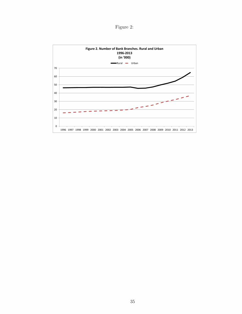
Figure 2:
0
10
20
30
40
50
60
70
1996 1997 1998 1999 2000 2001 2002 2003 2004 2005 2006 2007 2008 2009 2010 2011 2012 2013
Figure 2. Number of Bank Branches. Rural and Urban1996-2013
(in '000)Rural Urban
35

Figure 3:
0
10
20
30
40
50
60
1996 1998 2000 2002 2004 2006 2008 2010 2012
In p
erce
ntFigure 3. Share of Bank Lending. By Ownership
1996-2013SBI Group Foreign Regional Rural Private Other Public
36

Figure 4:
0
500
1000
1500
2000
2500
3000
3500
4000
4500
5000
1 2 3 4 5 6 7 8 9 10 11 12 13 14 15 16 17 18
Figure 4. Value of Lending. Rural and Urban Branches.1996-2013
(in '000 crores of rupees)Rural Urban
37

Figure 5:
0
100
200
300
400
500
600
700
800
900
1996 1997 1998 1999 2000 2001 2002 2003 2004 2005 2006 2007 2008 2009 2010 2011 2012 2013
Figure 5. Number of Loans. Rural and Urban Branches1996-2013
(in lakhs, or 100,000)Rural Urban
38

Figure 6:
0
100
200
300
400
500
600
700
800
900
1000
1996 1997 1998 1999 2000 2001 2002 2003 2004 2005 2006 2007 2008 2009 2010 2011 2012 2013
Figure 6. Average Ticket Size. Rural and Urban Branches1996-2013
(in '000 of rupees)Rural Urban
39

Figure 7:
0
2
4
6
8
10
12
14
16
Figure 7. Cash Reserve Ratio1996-2013
40

Figure 8:
0
1
2
3
4
5
6
7
8
9
10
Figure 9. Policy Repo Rates. 1996-2013
policy repo rate reverse repo rate
41

Table 1: Analysis of Variance of Log(lending)
[1] [2] [3] [4]In % 1996 2005 2009 2013
Between banks 27 24 18 10Within banks 73 76 82 90
Within districtIn %
Between banks 14 15 16 9Within banks 86 85 84 91
42

Table 2: Sample of Banks
Panel A: Bank Characteristics, 2013
Lending ShareNumber (INR 10 billion) in %
All Banks 150 37 100Public 26 156.5 74Private 20 52.5 19Foreign 40 6.6 5Regional Rural 64 2.1 2
Panel B: Bank and Branch Characteristics
Bank-level Branch-levelLending Lending
Number (INR 10 billion) Number (INR thousands)
1996 283 0.9 62,465 40,7741997 297 1.0 63,088 45,0751998 298 1.1 63,734 51,7691999 299 1.3 64,364 60,0862000 296 1.6 65,004 71,4372001 296 1.8 65,406 82,8912002 292 2.3 65,608 99,9872003 286 2.6 65,975 114,5842004 285 3.1 66,498 132,3822005 282 4.1 67,519 170,6882006 217 7.0 68,178 222,0432007 178 10.9 69,720 279,2742008 168 14.4 72,914 331,4872009 163 17.5 77,972 365,2232010 162 20.6 82,136 407,2722011 161 25.3 86,556 470,8682012 164 29.3 93,564 513,3672013 150 36.8 101,603 543,814
43

Table 3: Coefficient of Variation: State Bank of India
All branches Within Mumbai district
Ticket size (in INR ’000) 13.1 3.6Credit to deposit ratio (in %) 79.1 8.6Share of NPAs 1.8 3.4Share of long-term loans 0.3 0.5Number of officers 2.1 2.5Clerks/officer ratio 0.5 0.4Deposits (in INR ’000) 3.1 2.2Rural dummy 0.7 -Interest rate spread -1.4 -0.8
44
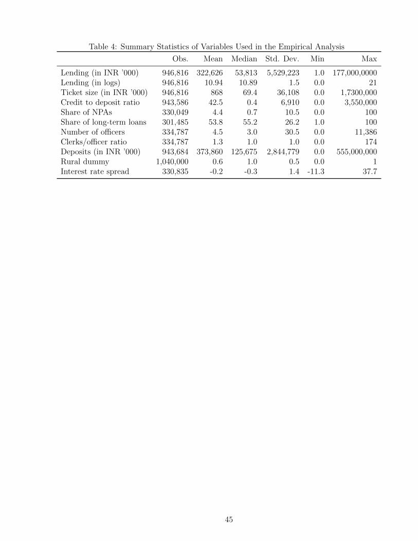
Table 4: Summary Statistics of Variables Used in the Empirical Analysis
Obs. Mean Median Std. Dev. Min Max
Lending (in INR ’000) 946,816 322,626 53,813 5,529,223 1.0 177,000,0000Lending (in logs) 946,816 10.94 10.89 1.5 0.0 21Ticket size (in INR ’000) 946,816 868 69.4 36,108 0.0 1,7300,000Credit to deposit ratio 943,586 42.5 0.4 6,910 0.0 3,550,000Share of NPAs 330,049 4.4 0.7 10.5 0.0 100Share of long-term loans 301,485 53.8 55.2 26.2 1.0 100Number of officers 334,787 4.5 3.0 30.5 0.0 11,386Clerks/officer ratio 334,787 1.3 1.0 1.0 0.0 174Deposits (in INR ’000) 943,684 373,860 125,675 2,844,779 0.0 555,000,000Rural dummy 1,040,000 0.6 1.0 0.5 0.0 1Interest rate spread 330,835 -0.2 -0.3 1.4 -11.3 37.7
45
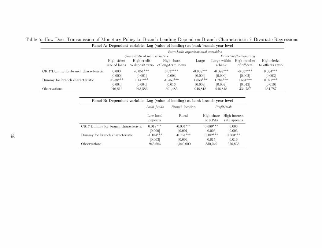
Table 5: How Does Transmission of Monetary Policy to Branch Lending Depend on Branch Characteristics? Bivariate RegressionsPanel A: Dependent variable: Log (value of lending) at bank-branch-year level
Intra-bank organizational variablesComplexity of loan structure Expertise/bureaucracy
High ticket High credit High share Large Large within High number High clerkssize of loans to deposit ratio of long-term loans a bank of officers to officers ratio
CRR*Dummy for branch characteristic 0.000 -0.051*** 0.037*** -0.038*** -0.028*** -0.057*** 0.034***[0.000] [0.001] [0.003] [0.000] [0.000] [0.002] [0.003]
Dummy for branch characteristic 0.938*** 1.147*** -0.469*** 1.853*** 1.784*** 1.551*** 0.071***[0.004] [0.004] [0.016] [0.003] [0.003] [0.012] [0.016]
Observations 946,816 943,586 301,485 946,818 946,818 334,787 334,787
Panel B: Dependent variable: Log (value of lending) at bank-branch-year level
Local funds Branch location Profit/risk
Low local Rural High share High interestdeposits of NPAs rate spreads
CRR*Dummy for branch characteristic 0.018*** -0.004*** 0.089*** 0.003[0.000] [0.001] [0.003] [0.003]
Dummy for branch characteristic -1.184*** -0.754*** 0.182*** 0.363***[0.003] [0.004] [0.015] [0.016]
Observations 943,684 1,040,000 330,049 330,835
46

Table 6: Transmission versus Branch Characteristics? Multivariate Regressions
Dependent variable: Log (value of lending) at bank-branch-year level
Intra bank organizational variablesCRR*Branch with high ticket size loans 0.039***
[0.003]CRR*Branch with high credit to deposit ratio -0.033***
[0.002]CRR*Branch with high share of long-term loans 0.027***
[0.002]CRR*Branch with high number of officers -0.099***
[0.002]Local fundsCRR*Branch with low deposits 0.011***
[0.003]Geographical locationCRR*Rural branch -0.006**
[0.002]Profits/RiskCRR*High interest rate spreads 0.047***
[0.002]CRR*Branch with high share of NPAs 0.026***
[0.002]
47
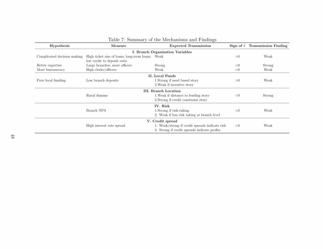
Table 7: Summary of the Mechanisms and FindingsHypothesis Measure Expected Transmission Sign of δ Transmission Finding
I. Branch Organization VariablesComplicated decision making High ticket size of loans; long-term loans; Weak >0 Weak
low credit to deposit ratioBetter expertise Large branches; more officers Strong <0 StrongMore bureaucracy High clerks/officers Weak >0 Weak
II. Local FundsPoor local funding Low branch deposits 1.Strong if need based story >0 Weak
2.Weak if incentive story
III. Branch LocationRural dummy 1.Weak if distance to lending story <0 Strong
2.Strong if credit constraint story
IV. RiskBranch NPA 1.Strong if risk-taking >0 Weak
2. Weak if less risk taking at branch level
V. Credit spreadHigh interest rate spread 1. Weak/strong if credit spreads indicate risk >0 Weak
2. Strong if credit spreads indicate profits
48

Table 8: Transmission of Monetary Policy to Branch Lending – Overall Effect
Dependent variable: Log (value of lending) at bank-branch-year level
CRR -0.210***[0.004]
Intra bank organizational variablesCRR*Branch with high ticket size loans 0.052***
[0.002]CRR*Branch with high credit to deposit ratio -0.047***
[0.002]CRR*Branch with high share of long-term loans 0.037***
[0.002]CRR*Branch with high number of officers -0.035***
[0.003]Local fundsCRR*Branch with low deposits 0.014***
[0.003]Geographical locationCRR*Rural branch -0.016***
[0.003]Profits/riskCRR*High interest rate spreads 0.050***
[0.002]CRR*Branch with high share of NPAs 0.025***
[0.002]
49

Table 9: How Does Transmission of Monetary Policy to Branch Lending Depend on BranchCharacteristics? State-Owned and Private Banks.
Dependent variable: Log (value of lending) at bank-branch-year levelState-Owned Banks Private Banks
Intra bank organizational variablesCRR*Branch with high ticket size loans 0.023*** 0.152***
[0.002] [0.016]CRR*Branch with high credit to deposit ratio -0.024*** -0.080***
[0.002] [0.012]CRR*Branch with high share of long-term loans 0.023*** 0.086***
[0.002] [0.015]CRR*Branch with high number of officers -0.090*** -0.155***
[0.002] [0.015]Local fundsCRR*Branch with low deposits 0.010*** 0.010
[0.003] [0.013]Geographical locationCRR*Rural branch -0.028*** 0.111***
[0.002] [0.014]Profits/riskCRR*High interest rate spreads 0.042*** 0.074***
[0.002] [0.019]CRR*Branch with high share of NPAs 0.003 0.208***
[0.002] [0.013]
50

Table 10: How Does Transmission of Monetary Policy to Branch Lending Depend on BranchCharacteristics? Episodes of Tightening and Loosening.
Dependent variable: Log (value of lending) at bank-branch-year levelTightening Loosening
Intra bank organizational variablesCRR*Branch with high ticket size loans -0.334*** 0.063***
[0.058] [0.007]CRR*Branch with high credit to deposit ratio 0.222*** -0.106***
[0.046] [0.006]CRR*Branch with high share of long-term loans -0.192*** 0.045***
[0.055] [0.006]CRR*Branch with high number of officers 0.191*** -0.125***
[0.057] [0.006]Local fundsCRR*Branch with low deposits -0.173*** 0.055***
[0.059] [0.007]Geographical locationCRR*Rural branch 0.009 -0.031***
[0.051] [0.007]Profits/riskCRR*High interest rate spreads -0.176*** -0.009
[0.061] [0.006]CRR*Branch with high share of NPAs -0.223*** -0.016**
[0.056] [0.006]
51

Table 11: How Does Transmission of Monetary Policy to Branch Lending Depend on BranchCharacteristics? Alternative Samples.
Dependent variable: Log (value of lending) at bank-branch-year levelDrop SBI Include RRBs
Costs of lending/supply capacityCRR*Branch with high ticket size loans 0.050*** 0.041***
[0.003] [0.002]CRR*Branch with high credit to deposit ratio -0.035*** -0.049***
[0.003] [0.002]CRR*Branch with high share of long-term loans 0.023*** 0.023***
[0.003] [0.002]CRR*Branch with high number of officers -0.111*** -0.096***
[0.003] [0.002]Local fundsCRR*Branch with low deposits 0.012*** 0.016***
[0.003] [0.002]Geographical locationCRR*Rural branch -0.004 -0.003ˆ
[0.003] [0.002]Profits/riskCRR*High interest rate spreads 0.042*** 0.043***
[0.003] [0.002]CRR*Branch with high share of NPAs 0.026*** 0.022***
[0.003] [0.002]
52

Table 12: How Does Transmission of Monetary Policy to Branch Lending Depend on BranchCharacteristics? Omitted Variables.
Dependent variable: Log (value of lending) at bank-branch-year levelElections Other Macroeconomic
Variables
Costs of lending/supply capacityCRR*Branch with high ticket size loans 0.039*** 0.044***
[0.003] [0.003]CRR*Branch with high credit to deposit ratio -0.033*** -0.036***
[0.002] [0.002]CRR*Branch with high share of long-term loans 0.027*** 0.030***
[0.002] [0.002]CRR*Branch with high number of officers -0.099*** -0.104***
[0.002] [0.002]Local fundsCRR*Branch with low deposits 0.011*** 0.012***
[0.003] [0.003]Geographical locationCRR*Rural branch -0.007*** -0.008***
[0.002] [0.003]Profits/riskCRR*High interest rate spreads 0.047*** 0.047***
[0.002] [0.002]CRR*Branch with high share of NPAs 0.026*** 0.026***
[0.002] [0.002]
53

Table 13: How Does Transmission of Monetary Policy to Branch Lending Depend on BranchCharacteristics? Omitted Variables (contd.).
Dependent variable: Log (value of lending) at bank-branch-year level
Costs of lending/supply capacityCRR*Branch with high ticket size loans 0.022*** 0.045***
[0.003] [0.005]CRR*Branch with high credit to deposit ratio -0.020*** -0.032***
[0.002] [0.004]CRR*Branch with high share of long-term loans 0.021*** 0.028***
[0.002] [0.005]CRR*Branch with high number of officers -0.081*** -0.132***
[0.002] [0.005]Local fundsCRR*Branch with low deposits 0.004 0.002
[0.002] [0.005]Geographical locationCRR*Rural branch -0.001 -0.027***
[0.002] [0.005]Profits/riskCRR*High interest rate spreads 0.055*** 0.011**
[0.003] [0.005]CRR*Branch with high share of NPAs 0.034*** -0.021***
[0.002] [0.005]
54

Table 14: How Does Transmission of Monetary Policy to Branch Lending Depend on Branch Characteristics? Dynamic Specifications
One-year lagged CRR First difference Lagged dependentin lending and CRR variable
Dependent variable: Log First difference of Log(value of lending) Log (value of lending) (value of lending)
Intra bank organizational variablesCRR*Branch with high ticket size loans 0.052*** 0.009*** 0.027***
[0.002] [0.001] [0.002]CRR*Branch with high credit to deposit ratio -0.036*** -0.007*** -0.002*
[0.001] [0.001] [0.001]CRR*Branch with high share of long-term loans 0.012*** 0.001 0.009***
[0.002] [0.001] [0.001]CRR*Branch with high number of officers -0.027*** -0.013*** -0.025***
[0.002] [0.001] [0.001]Local fundsCRR*Branch with low deposits 0.010*** 0.009*** -0.012***
[0.002] [0.001] [0.002]Geographical locationCRR*Rural branch 0.056*** -0.006*** -0.034***
[0.002] [0.001] [0.002]Profits/RiskCRR*High interest rate spreads -0.027*** -0.004*** 0.018***
[0.002] [0.001] [0.001]CRR*Branch with high share of NPAs -0.022*** -0.010*** 0.010***
[0.002] [0.001] [0.001]
55


