
The metal content of hot DA white dwarf spectra
Nathan James Dickinson
Supervisor:
Martin Barstow
A thesis submitted for the degree of Doctor of Philosophy
at the University of Leicester
March 2012

I
Declaration
I hereby declare that no part of this thesis has been previously submitted to this or any other University as part of the requirement for a higher degree. The work described herein was conducted by the undersigned, except for contributions from colleagues as acknowledged in the text.
Nathan James Dickinson March 2012

II
The metal content of hot DA white dwarf spectra
Nathan James Dickinson
ABSTRACT
In this thesis, a study of the high ionisation-stage metal absorption features in the spectra of hot DA white dwarfs is presented. Metals are present in the photospheres of such stars due to radiative levitation (Chayer et al. 1994, 1995; Chayer Fontaine & Wesemael 1995). However, studies of the patterns between metal abundance and Teff show that, though the broad patterns predicted are seen, individual abundance measurements often do not reflect the predictions of radiative levitation theory (e.g. Barstow et al. 2003b). In this thesis, an analysis of the nitrogen abundance in three stars is performed, where a highly abundant layer of nitrogen was thought to reside at the top of the photospheres of the stars. The nitrogen abundance and distribution in these DAs is found to be homogeneous and of an abundance in keeping with stars of higher Teff.
The accretion of metals from circumstellar discs has been shown to be the source of photospheric metals in DAs with Teff < 25,000 K (e.g. Zuckerman et al. 2003), where gravitational diffusion dominates (Koester & Wilken, 2006). In some cases, gaseous components are seen at such discs (e.g. SDSS 122859.93+104032.9; Gänsicke et al. 2006). A survey is made of a sample of hot (19,000 K < Teff < 51,000 K) DAs, where similar accretion may explain the inability of radiative levitation theory alone to account for the detected photospheric metal abundances. No circumstellar gas discs are found, though accretion from as yet undetected circumstellar sources remains an attractive explanation of the photospheric abundances of the stars.
Circumstellar absorption is seen in the UV spectra of some hot DA stars (Holberg et al. 1998; Bannister et al. 2003). Sources suggested for this material include circumstellar discs, the ionisation of the ISM, stellar mass loss and planetary nebulae. A re-analysis of this absorption is presented, using a technique that for the first time allows proper modelling of the circumstellar absorption features, and provides column densities for all components. The ionisation of circumstellar discs or planetesimals, the ionisation of the ISM and the ionisation of mass lost by binary companions are put forward as the origin for this circumstellar material.

III
Publications
A significant amount of work contained in this thesis has been published in the following papers: “On the Origin of Metals in Some Hot White Dwarf Photospheres,” Burleigh M.R., Barstow M.A., Farihi J., Bannister N.P., Dickinson N.J., Steele P.R., Dobbie P.D., Faedi F., Gänsicke B.T., 2010, in ‘17th European White Dwarf Workshop,’ eds. Werner K., Rauch T., AIP Conference Proceedings, Vol. 1273, p. 473 “On the Origin of Metals in Some Hot White Dwarf Photospheres,” Burleigh M.R., Barstow M.A., Farihi J., Bannister N.P., Dickinson N.J., Steele P.R., Dobbie P.D., Faedi F., Gänsicke B.T., 2011 in ‘Planetary Systems Beyond the Main Sequence’, eds. Schuh S., Dreschel H., Heber U., AIP Conference Proceedings, Vol. 1331, p. 289 “On the Origin of Metals in Some Hot White Dwarf Photospheres,” Burleigh M.R., Barstow M.A., Farihi J., Bannister N.P., Dickinson N.J., Steele P.R., Dobbie P.D., Faedi F., Gänsicke B.T., 2012, MNRAS, in preparation “The Stratification of Metals in Hot DA White Dwarfs Atmospheres,” Dickinson N.J., Barstow M.A., Hubeny I., 2010, in ‘17th European White Dwarf Workshop,’ eds. Werner K., Rauch T., AIP Conference Proceedings, Vol. 1273, p. 400 “The distribution of metals in hot DA white dwarfs,” Dickinson N.J., Barstow M.A., Hubeny I., 2012, MNRAS, 421, 3222 “The origin of circumstellar features in the spectra of hot DA white dwarfs,” Dickinson N.J., Barstow M.A., Welsh B.Y., Burleigh M., Farihi J., Redfield S., Unglaub K., MNRAS, 2012, in press

IV
Acknowledgements
The work contained in this thesis could not have been possible without the help of many other people. Obviously, I have a lot to thank Martin for, for helping me become a (good?) scientist, opening my eyes to the fascinating area that is white dwarf astronomy, and for fully supporting me along the way. The other staff in the white dwarf group at Leicester also shoulder some blame; thanks to Matt for a great observing experience in La Palma, and for always knowing where to drink, no matter what city or what country we happen to be in (“this beer tastes like bacon!”); Sarah has been a great source of help, and has never made me feel stupid, even when I’ve asked stupid questions; thanks to Jay for both showing me around Hawaii and for all the help he’s given me in the later study of this thesis. Thanks also to Paul, Dave, Katherine and Simon. All of these people, plus those who I have met on my travels, have shown me that a career in science is truly worthwhile. I’d also like to thank Ivan Hubeny for his help in getting my white dwarf modelling skills to a decent standard. Barry Welsh has contributed a lot to my understanding of the ISM and has opened my eyes to wealth of possibilities that exist in reality TV, should my astronomy career not work out. Similarly, Seth Redfield and Klaus Unglaub have been important in shaping my understanding of the LISM and white dwarf mass loss. The quality of the work here would be far from what it is now without the guidance and help of all. I’d also like to thank the other PhD students in the X-ray and Observational Astronomy and Theoretical Astrophysics Groups, for being good sports during teatime rants. I would never have achieved what I have done, had I not had the support of my parents, Andrew and Joy, from day one; they made me realise there is no limit to the reward of hard work, and that you can do anything you want to. Thank you. Credit should also be given to my brother, Luke; no matter how sincerely I try to explain what I do, I’ll always get a laugh (“so what do you actually do all day?”) Last, but by no means least, I’d like to thank Sophia, for enduring the non-existent weekends and evenings, and the tantrums when things don’t work. Together, anything is possible.
V
For Sophia
VI
Contents. 1. Introduction. 1
1.1. White dwarfs – an overview. 1
1.2. The discovery of white dwarfs. 3
1.3. The structure of white dwarfs. 5
1.4. White dwarf classification. 7
1.5. White dwarf formation. 9
1.6. White dwarf evolution. 13
1.7. Metals in DA spectra. 15
1.7.1. The case of hot DA stars. 16
1.7.2. The stratification of metals in hot DAs. 19
1.7.3. Circumstellar material at hot DA stars. 29
1.8. Modelling white dwarf stars. 37
1.9. Structure of thesis. 39
1.10. Summary. 40
2. Instruments and white dwarfs studied. 42
2.1. Introduction. 42
2.2. The Space Telescope Imaging Spectrograph (STIS). 42
2.3. The Goddard High resolution Spectrograph (GHRS). 43
2.4.The Intermediate dispersion Spectrograph and Imaging System (ISIS). 44
2.5. The Far Ultraviolet Spectroscopic Explorer (FUSE). 44
2.6. The Extreme Ultraviolet Explorer (EUVE). 47
2.7. The International Ultraviolet Explorer (IUE). 47

VII
2.8. White dwarfs studied. 48
3. Stratified metals in hot white dwarf atmospheres? 51
3.1. Introduction. 51
3.2. Observations and method. 52
3.3. WD 1029+537. 55
3.4. WD 1611–084. 57
3.5. WD 0050–332. 58
3.6. WD 0948+534. 59
3.7. Discussion. 59
3.8. Summary. 67
4. A search for circumstellar gas disks at hot white dwarfs. 69
4.1. Introduction. 69
4.2. Observations and data reduction. 70
4.3. Results. 71
4.4. Discussion. 71
4.5. Summary. 76
5. The origin of ‘circumstellar’ features in hot white dwarf spectra 78
5.1. Introduction. 78
5.2. Observations and modelling circumstellar components. 79
5.3. Results. 83
5.3.1. Summary of results. 83
5.3.2. Objects with circumstellar absorption. 85

VIII
5.3.2.1. WD 0232+035 (Feige 24). 85
5.3.2.2. WD 0455–282 (REJ 0457–281). 86
5.3.2.3. WD 0501+527 (G191-B2B). 88
5.3.2.4. WD 0556–375 (REJ 0558–373). 89
5.3.2.5. WD 0939+262 (Ton 021). 89
5.3.2.6. WD 1611–084 (REJ 1614–085). 90
5.3.2.7. WD 1738+665 (REJ 1738+665). 91
5.3.2.8. WD 2218+706. 92
5.3.3. Objects without circumstellar absorption. 93
5.3.3.1. WD 0050–335 (GD 659). 93
5.3.3.2. WD 0621–376 (REJ 0623–371). 93
5.3.3.3. WD 0948+548 (PG 0948+534). 94
5.3.3.4. WD 1029+537 (REJ 1032+532). 98
5.3.3.5. WD 1057+719 (PG 1057+719). 99
5.3.3.6. WD 1123+189 (PG 1123+189). 99
5.3.3.7. WD 1254+223 (GD 153). 99
5.3.3.8. WD 1314+293 (HZ 43). 100
5.3.3.9. WD 1337+705 (EG 102). 100
5.3.3.10. WD 2023+246 (Wolf 1346). 101
5.3.3.11. WD 2111+498 (GD 394). 101
5.3.3.12. WD 2152–548 (REJ 2156–546). 102
5.3.3.13. WD 2211–495 (REJ 2214–492). 102
5.3.3.14. WD 2309+105 (GD 246). 103
5.3.3.15. WD 2331–475 (REJ 2334–471). 103
5.4. Discussion. 104

IX
5.4.1. Circumstellar disks. 106
5.4.2. Ionised ISM. 108
5.4.3. White dwarf mass loss. 117
5.4.4. Planetary nebula material. 123
5.5. Summary. 125
6. Conclusions and suggestions for further work. 129
6.1. Introduction. 129
6.2. Concluding remarks and suggestions for further work. 129
A Chapter 6: Tables of DA and solar metal abundances used for mass loss 138
calculations.
Bibliography 141

X
List of figures.
1.1
1.2
1.3
1.4
1.5
An image of the Sirius binary system, taken using the Hubble Space
Telescope's Wide Field Planetary Camera 2. The white dwarf, Sirius
B, is the smaller of the two stars, to the lower left of the larger star,
Sirius A. Image credit: NASA, ESA, H. Bond (STScI) and M.
Barstow (University of Leicester).
The Hertzsprung-Russell diagram, including the positions of Sirius B
and Procyon B (image from
http://www.daviddarling.info/encyclopedia/H/HRdiag.html).
The Hertzsprung-Russell diagram, illustrating the evolution of a solar
type star (from Marsh 1995).
The Helix Nebula (NGC 7293), with the white dwarf WD 2226–210
at its centre. Image credit: NASA, WIYN, NOAO, ESA, Hubble
Helix Nebula Team, M. Meixner (STScI) & T.A. Rector (NRAO).
The N V resonance doublet of WD 1029+537 (Figure 5, Holberg et
al. 1999a). A layer of nitrogen in the topmost part of the atmosphere
(!M/M = 3.1x10⁻¹⁶) is illustrated with the upper curve. A
homogeneous nitrogen distribution (log(N/H) = –4.31) is shown with
the lower curve.
4
8
11
13
23

XI
1.6
1.7
1.8
1.9
1.10
The EUVE spectrum of WD 1029+537 (Figure 6, Holberg et al.
1999a). The homogeneous model is again shown by the lower curve
and the stratified nitrogen configuration is indicated with the upper
curve.
Measured nitrogen abundance as a function of Teff (Figure 10,
Barstow et al. 2003b). WD 1029+537, WD 1611–084 and WD 0050–
332 are the three objects with Teff < 50,000 K with nitrogen
detections.
Figure 1 from Schuh, Barstow & Dreizler 2005. A comparison of the
nitrogen abundances using the stratified models of Schuh, Dreizler &
Wolff (2002; light grey data points) to the measurements of Barstow
et al. (2003b; black data points). The radiative levitation predictions
of Chayer et al. (1995) are denoted with dark grey symbols, while the
cosmic abundance is shown with the dotted line.
Figure 1 from Chayer, Vennes & Dupuis 2005. A comparison of the
N/H values found by Chayer, Vennes & Dupuis (open circles) to
those found by Barstow et al. (2003b; filled circles).
The C IV doublet in the STIS spectrum of WD 0948+534 has narrow,
deep absorption lines, like the N V doublet of WD 1029+537.
24
25
26
27
28

XII
1.11
2.1
3.1
3.2
3.3
Figure 1 from Gänsicke et al., 2008. The left hand panel shows the
photospheric Mg II (4481 Å) absorption lines in the William
Herschel Telescope (WHT) spectra of WD1337+705, SDSS 1228 and
SDSS 1043 (black lines), with the best fitting white dwarf models
(grey). The right panel shows the 8350 – 8800 Å region of the spectra
of WD 1337+705, GD 362, SDSS 1228 and SDSS 1043, normalised
and offset for clarity. WHT spectra are shown in black, while the
SDSS spectra are plotted in grey.
Two WD 0501+527 FUSE spectra, showing the 'region of the worm'.
The upper panel shows the 1BLiF spectrum from observation
M1010201000 (13th October 1999 01:25:31) and the lower panel is
from observation M1030602000 (21st November 1999 11:39:56).
The best fitting model (N/H = 3.39x10⁻⁷) of the N V doublet of WD
1029+537.
The EUVE SW data for WD 1029+537 fit with a homogeneous
nitrogen distribution with N/H = 3.39x10⁻⁷.
The lower nitrogen abundance model (N/H = 1.76x10⁻⁶,
!"2 = 1.21)
of WD 1611–084 is shown in the upper panel. The lower panel shows
the high abundance model (N/H = 3.41x10⁻⁴;
!"2 = 1.13).
34
46
56
56
57

XIII
3.4
3.5
The best fitting model (N/H = 6.05x10⁻⁷,
!"2 = 2.15) of the N V
doublet of WD 0050–332.
The N V doublet of WD 0948+534, fit with a model with
N/H = 1.6x10⁻⁶.
58
60
3.6
The
!"2 distribution of WD 1029+537 as N/H is increased. The global
minimum is represented with a dashed line, and its three ! confidence
limit is denoted with a dotted line.
62
3.7 The
!"2 distribution of WD 1611–084. The line representations are
the same as in the previous figure.
63
3.8
3.9
The change in the log of the ratio of the NLTE population responsible
for the N V doublet (2S) to the N VI level population, with nitrogen
abundance. Note that not all of the model grids span the same
abundance range; models were only computed over the range
required to explain the observations.
A comparison of the nitrogen abundances found here (triangles) to
those found by Barstow et al. (2003b; filled circles) and Chayer et al.
64
65
XIV
3.10
4.1
4.2
4.3
5.1
(2005; open circles). The dotted lines connect multiple measurements
of individual stars for ease of comparison.
A comparison of the N/H values found here, by Barstow et al.
(2003b) and Chayer et al. (2005), to the radiative levitation
predictions of Chayer et al. (1995). The plot symbols are the same as
in the previous figure.
The spectral region containing the Ca II triplet. Each data set is
normalised and offset for clarity.
The spectral region containing the Mg II 4482 Å absorption line. The
gaps in the spectrum of WD 1942+499 are due to the removal of
cosmic ray contamination.
The upper panel shows the Fe II absorption (5020 Å) in the spectrum
of WD 0209+085, while the bottom panel shows the Si III absorption
features (4552 Å, 4568 Å) in the spectrum of WD 2111+498.
The 1548 Å C IV line of WD 0232+025, where the binary phase is
0.24. The circumstellar component (at 7.4 km s-1) is blended with the
photospheric components (at 30.11 km s-1). The data is plotted with a
solid red line, the model components are plotted with dotted red lines
and the sum of the model components is plotted in blue; this plotting
convention is also used in Figures 5.2 – 5.4.
66
66
67
68
87

XV
5.2
5.3
5.4
5.5
5.6
5.7
5.8
The 1548 Å C IV line of WD 0232+025, where the binary phase is
0.74. The photospheric component at (128.23 km s-1) is not seen
here.
The 1548 Å component of the C IV doublet of WD 0948+534, fit
with an absorbing component at –16 km s–1.
The 1548 Å component of the C IV doublet of WD 0948+534, fit
with two absorbing components at –17.6 km s–1 and 1.65 km s–1.
The Si IV 1393 Å line fit with two absorbing components at –16.9
km s–1 and 3.5 km s–1.
A plot of vCSshift, with the shifts in the measured and predicted ISM
components (from Table 5.2). The measured velocity shifts are
plotted in black, while the predicted shifts in vLISM are plotted in grey.
In some cases the error bars are smaller than the plot symbols; the
symbols are open to allow the error bars to be seen.
The column densities measured in this study, with the column density
ranges predicted by Dupree & Raymond (1983) for a DA Strömgren
sphere (dashed lines).
A comparison of the mass loss calculations performed here using the
87
96
97
97
113
115
120
XVI
5.9
metal abundances in Appendix A (circles) to those of Bannister et al.
(2003; squares). The stars without circumstellar absorption lines are
the filled symbols, while the stars with circumstellar absorption are
plotted with open symbols. The stars are plotted from left to right in
order of decreasing Teff to show the trend seen by Bannister et al.
(2003).
A comparison of the vphot–vCS values here (triangles) to the vexp
measurements from Napiwotzki & Schönberner (1995; circles). Since
no nebula radius measurements exist for the stars in this sample, the
vphot–vCS values are plotted at zero pc. Overlapping values are offset
for clarity, and the values for WD 2218+706 are labelled.
124

XVII
List of tables.
1.1
1.2
1.3
2.1
3.1
The white dwarf classification system.
Individual white dwarfs discussed in the introduction to this thesis, their
properties, location in the introduction and relevant references. ‘CS’
signifies ‘circumstellar.’
The metal absorption/emission lines discussed in throughout this thesis,
with their laboratory wavelengths (in Å). Included are the low ion
absorption features that are used to characterise the ISM in Chapter 5.
The features are grouped according to their origin. All wavelengths are
taken from the Kurucz database.
The white dwarfs studied here, their stellar parameters, the chapters in
which they are investigated, interesting properties and sources of data.
The observation information, stellar and ISM parameters for the white
dwarfs studied here (unless stated otherwise, all data are from Barstow
et al. 2003b). The absence of data signifies where a measurement was
unobtainable, either due to lack of spectral coverage or an inability to
model the absorption features.
9
17
18
49
54

XVIII
3.2
3.3
3.4
4.1
5.1
5.2
5.3
5.4
The laboratory wavelengths of the FUV absorption features examined
here.
The estimated metal abundances for WD 0948+534. Given the poor
match to the data, errors were not computed for these models.
The best fitting nitrogen abundances for WD 1029+537, WD 1611–084
and WD 0050–332 adopted in this study.
The white dwarfs observed in this study. The right ascension (RA) and
declination (DEC) (J2000) of each star are from the McCook & Sion
online catalog. The Teff values are from the references detailed.
The stellar parameters and observation information for the DAs studied
here.
All measured velocities, circumstellar velocity shift (vCSshift), predicted
LISM velocities and gravitation redshifts (vgrav). All velocities are
expressed in km s-1.
The stars with circumstellar detections, the identified species and
measured column densities.
The key differences between the findings of this study and that of
Bannister et al. (2003).
55
59
61
70
80
84
85
105

XIX
5.5
5.6
The metal column densities for a range of ISM models (Table 1,
Indebetouw & Shull, 2004). All column densities are expressed in units
of 1012 cm–2.
The estimated rS (from Tat & Terzian, 1999) for each of the DAs with
circumstellar absorption, and estimated distances (D) to the absorbing
material (for ne = 0.01 and 0.03 cm!3). D was calculated by subtracting
rS from the distance to the star (from Table 5.1). The ISM component
with a velocity matching vCS is stated; a ‘?’ denotes the tentative
association with the Hyades cloud. All rS and D values are expressed in
pc.
114
116
A1 A2
Hot white dwarf metal abundances.
The solar metal abundances reported by Asplund et al. 2009.
139 140

1
Chapter 1.
Introduction.
1.1. White dwarfs - an overview.
After stars like the Sun have finished their nuclear burning and have expelled
their outer layers, the degenerate, cooling stellar core remains. This remnant core is a
white dwarf. White dwarfs typically have radii similar to that of the Earth, and have
masses around 0.6 solar masses (M!
). This small radius gives these objects
extraordinarily high densities, making them astronomical ‘compact objects,’ a title
shared only with neutron stars and stellar mass black holes. Being the evolutionary
end point of stars with initial masses ! 8 M!
(e.g. Weidemann 1987; Casewell et al.
2009), approximately 98% of stars will end their lives as white dwarfs (e.g. Wood
1992).
White dwarfs have a variety of applications in astronomical studies. As the end
states of the evolution of the majority of stars, white dwarfs are of massive
importance to our understanding of the life cycle of most of the stars in the Universe.
Signatures of processes that occurred in earlier phases of the star’s life are exhibited
by the white dwarf, and thus these objects allow us to understand not just the end state
of stellar evolution they represent, but also previous stages of the star’s life. The

2
pollution of white dwarfs by circumstellar planetary debris discs (discussed in more
detail in Section 1.7.3) can be used to probe the end points of planetary system
evolution, and indeed the ultimate fate of the Sun and Solar System.
Although the subject of this thesis is the metal features in white dwarf spectra,
broadly speaking white dwarfs are thought of as having ‘pristine’ atmospheres. Due to
their exceedingly high surface gravity (log g ~7–9), the early view was that all
elements but the lightest atmospheric constituent (i.e. hydrogen and/or helium) diffuse
downward to leave a smooth continuum spectrum with no spectral features other than
H or He (e.g. Schatzmann 1958). By examining interstellar medium (ISM) absorption
features superimposed over the white dwarf continuum, these objects are often used to
probe the structure and ionisation state of the ISM (e.g. Barstow et al. 2010; Redfield
& Linsky, 2002, 2004a,b, 2008). Given their simple spectral form, white dwarfs are
also often used as calibration targets for astronomical observations (e.g. Bohlin et al.
2011; Bohlin, Dickinson & Calzetti, 2001).
Being among the oldest stellar objects, white dwarfs can be used to determine
the age of stellar populations, and as such can be used to provide an age estimate for
the Galactic disc (e.g. Fontaine, Brassard & Bergeron, 2001). Given the use of
supernovae as ‘standard candles’ in extragalactic astronomy, better understanding of
white dwarfs as possible Type Ia supernova progenitors (e.g. Maxted et al. 2000) will
allow a better understanding of the cosmological distance ladder and dark energy (it
must be stressed that although white dwarfs are thought to be viable Type Ia
supernova progenitors, a detailed understanding of the precise mechanism(s) is still a
work in progress). White dwarfs are interesting not just to the astronomer; the interior

3
of a white dwarf contains matter of a phenomenal density, making these objects
unique physical laboratories.
1.2. The discovery of white dwarfs.
William Herschel was the first person to observe a white dwarf, discovering the
star 40 Eridani (Eri) B (WD 0413–074) in 1783. However, he did not immediately
notice anything untoward about the star. Almost fifty years later, in 1834, Friedrich
Bessel noted the oscillating proper motion of Sirius (the dog star), hinting that a
binary companion was present; a similar observation was made of the star Procyon
(Bessel, 1844). Using subsequent observations, Peters first calculated the orbital
elements of the Sirius binary in 1851 (Peters, 1851). Some 11 years later, Clarke first
imaged Sirius B (WD 0642–166; Figure 1.1) using the 18.5 inch refracting telescope
he was testing for the Dearborn Observatory, at the time the largest telescope in the
USA. Bond officially reported this discovery later that year, after having observed the
star himself at the Observatory of Harvard College (Bond, 1862).
The exotic and enigmatic nature of white dwarf stars began to emerge shortly
after the discovery of Sirius B. The Russian astronomer Otto Struve determined that
Sirius B has a mass of around half that of Sirius A, and reasoned that given they are at
the same distance, Sirius B ought to be a 1st magnitude star with a radius 80% of that
of Sirius A, if both stars are made of the same material (Struve, 1866). Since Sirius B
was found to be an 8th magnitude star with a diminutive radius, Struve postulated that
Sirius A and B are of “a very different physical constitution.”

4
Figure 1.1. An image of the Sirius binary system, taken using the Hubble Space
Telescope's Wide Field Planetary Camera 2. The white dwarf, Sirius B, is the smaller
of the two stars, to the lower left of the larger star, Sirius A. Image credit: NASA,
ESA, H. Bond (STScI) and M. Barstow (University of Leicester).
Much later, in 1915, Adams obtained a spectrum of Sirius B at the Mount
Wilson Observatory. The star was found to have an effective temperature (Teff)
around 29,000 K, almost three times greater than Sirius A, though it was almost 1,000
times less luminous (Adams, 1915). Spectra of 40 Eri B and Procyon B (WD
0736+053) revealed a similar situation in those systems. Physical theories at the time
required that hotter stars had a far greater luminosity than cooler stars. The only
explanation for the observations was that the anomalous stars had radii approaching
that of the Earth, giving them densities 105–106 times greater than that of the Sun. No
contemporary physical theory could explain such an object, since according to the
astrophysics of the time such stars should undergo a gravitational collapse.
5
The first isolated white dwarf was discovered a few years later, by van Maanen
(van Maanen’s Star, WD 0046+051), in 1917 (van Maanen, 1917). Though originally
thought to be an F0 star (van Maanen, 1917), the star is actually of the DZ class, and
was therefore the first metal polluted white dwarf to be discovered. The source of
these metals is now understood to be due to the accretion of disrupted planetary debris
by the white dwarf (see Section 1.7.3 for a detailed discussion of this phenomenon).
The term white dwarf was not used until 1922, when it was coined by Luyten to
describe the white colour and small radii of these stars.
1.3. The structure of white dwarfs.
The matter making up these stars remained a mystery until the advent of
quantum mechanics, and Fermi and Dirac’s statistical theory of an electron gas in
1926. According to this theory, the behaviour of individual electrons inside an atom is
governed by quantum mechanics, and the electrons will only occupy discrete energy
levels. In materials with closely spaced atoms, the most loosely bound electrons can
move freely, and are considered to form a gas; this electron gas is responsible for the
conduction of heat and electricity in metals. However, the electron energy levels
remain quantised, and each electron will occupy the lowest energy level available to it
up to a maximum energy limit (the ‘Fermi energy’). Any states with the same energy
are ‘degenerate,’ and a gas such as this is said to be degenerate since all available
electron states are occupied. The ‘Pauli Exclusion Principle’ prevents any two
electrons sharing the exact same energy state.
6
In the extreme pressure environment of a white dwarf, the ions are compressed
so closely that their quantised electron energy structures are broken down; an electron
gas is again present. According to the Heisenberg Uncertainty Principle, !x!p " h/4#
(where !x is the position uncertainty and !p is the momentum uncertainty of a given
electron, and h is Planck’s constant), so that as this electron gas becomes compressed
!x decreases, raising !p. This in turn raises the pressure of the gas. Since, according
to the Pauli Exclusion principle, only two electrons (with opposite spin values) can
occupy a given position-momentum phase cell, such compression is resisted by this
‘degeneracy pressure.’ In 1926, Fowler showed that it is this outward degeneracy
pressure that provides a resistance to the gravitational collapse of a white dwarf.
A mere five years later, the noted Indian physicist Subrahmanyan
Chandrasekhar (nephew of the Nobel Prize winning C.V. Raman, after whom Raman
scattering is named) combined quantum mechanics with the theory of relativity and
derived the equations describing the structure of white dwarfs. He predicted both the
white dwarf mass-radius relation (R $ M–1/3, where R and M are the white dwarf
radius and mass, respectively) and that at some mass limit (1.4 M!
, the
Chandrasekhar mass), the outward degeneracy pressure in a non-rotating white dwarf
would be insufficient to support the weight of the star, and that the star would
undergo a violent gravitational collapse. It is a point of historical interest that
although many of Chandrasekhar’s contemporaries (including Bohr, Pauli and
Fowler) agreed with his theory, they did not initially publicly support him as the
eminent British astrophysicist Sir Arthur Eddington harshly rejected Chandrasekhar’s
work, stating that he thought “there should be a law of Nature to prevent a star from
behaving in this absurd way” (Meeting of the Royal Astronomical Society, 11th
7
January 1935, as reported in the Observatory, 1935). Chandrasekhar won the Nobel
Prize in 1983 for this work, died in 1995, and the Chandra X-ray observatory
(launched July 23rd, 1999) is named in his honour.
A white dwarf is commonly composed of a carbon and oxygen ions (leftover
from the helium burning processes in the progenitor star) and degenerate electron
plasma core. Typically, 99.99% of the mass of the object is contained within this core.
In cooler white dwarfs, with 4,000 K < Teff < 10,000 K, the cores of these stars
crystallise. Above this core lies a thin non-degenerate atmosphere, composed mainly
of hydrogen and/or helium.
1.4. White dwarf classification.
As far back as the Father Angelo Secchi’s attempts at stellar classification in
the 1860s, stars have been categorised using their spectral characteristics, culminating
in the Harvard classification system used today. White dwarfs are no exception.
Attempts to classify white dwarfs were begun by Kuiper (1941). Luyten (1952) found
that white dwarfs occupied a continuous, lower luminosity strip parallel to the main
sequence on the Hertzsprung-Russell diagram (Figure 1.2), leading to the white dwarf
classification system devised by Greenstein (1960); the prefix “D” (for degenerate),
followed by the Harvard spectral class for the star. Using this system, the hydrogen
dominated objects occupied the DA class, while the mainly helium rich stars occupied
the DB, DC, DF, DG, DK and DM classes. However, as white dwarf studies evolved
and many hybrid objects were discovered, the classification system became

8
unworkable; the system also gave no indication of a white dwarf’s Teff, which can
vary from a few thousand to ~150,000K.
Figure 1.2. The Hertzsprung-Russell diagram, including the positions of Sirius B and
Procyon B (image from http://www.daviddarling.info/encyclopedia/H/HRdiag.html).
This led Sion et al. (1983) to introduce the classification system for white
dwarfs that is still in use today. The new system retains the ‘D’ to signify the
degenerate nature of white dwarfs, followed by a symbol signifying the main
atmospheric constituent (more detail is given in Table 1.1). Though often dropped
when quoting a white dwarf’s class, a temperature index is also used, equal to
50,400 K divided by the Teff of the star. Hybrid classes are described using a mix of
symbols, in order of dominance, so a hydrogen dominated white dwarf with

9
secondary metal absorption features, a debris disc and a Teff of 16,800 K is a DAZd3.0
star.
Table 1.1. The white dwarf classification system.
Class Teff Range (K) Spectral Characteristics
H-rich DA 6,000–100,000 Balmer lines only, no He or metal features
DAO >45,000 Balmer lines and weak He II features
He-rich
DO 45,000–100,000 Strong He II lines, some He I present DB 12,000–30,000 HeI lines, no H or metals*
DBA 12,000–30,000 He I lines and weak Balmer lines present
Cool WDs
DQ 6,000–12,000; 18,000–24,000**
C features (atomic or molecular)
DZ <6,000†; 10,000‡ Metal lines only, no H or He
DC <6,000†; 10,000‡ Featureless continuum (no lines deeper than 5%)
Additional Secondary Feature P Magnetic with polarisation H Magnetic with no detectable polarisation
E Emission lines present
V Variable d Debris Disc
*note that some DB stars with 30,000 K < Teff < 45,000 K have been found in the ‘DB
gap’ (Kleinman et al. 2004); **these stars correspond to the ‘hot DQ’ stars (Liebert et
al. 2003; Dufour et al. 2008);†for a hydrogen atmosphere; ‡for a helium atmosphere.
1.5. White dwarf formation.
All stars with masses ! 8 M
!(e.g. Weidemann & Koester 1983; Weidemann
1987; Casewell et al. 2009), will end their lives as white dwarfs. Whilst on the stellar
main sequence (see Figure 1.2), stars produce their energy from the fusion of

10
hydrogen in their cores. The pressure from the radiation produced in this process
counteracts the downward gravitational force acting on the star, holding the star up at
a roughly constant radius; the star is in hydrostatic equilibrium. The amount of time a
star spends in this phase depends strongly on its mass; stars like the Sun will spend of
the order of ten billion years on the main sequence while stars ten times the mass of
the Sun will spend only 30 million years in this state. Eventually, all stars will run out
of useable hydrogen, leaving a helium core. The stellar core then contracts
(Schönberg & Chandrasekhar 1942). This contraction increases the temperature of the
core and the material surrounding it, since the temperature of a virialised mass is
proportional to the reciprocal of its radius.
The cores of white dwarfs come in three distinct varieties, depending upon the
initial mass of the progenitor star and its evolution. Stars with an initial mass < 0.5
M!
never become hot enough to fuse helium into metallic elements, and are thus
expected to evolve into stars with helium cores. The time for this process takes longer
than a Hubble time (Laughlin et al. 1997) for single star evolution, leading to the
assertion that the observed helium core white dwarf population must be the result of
binary mass transfer (e.g. Liebert et al. 2004), where much of the mass of the
progenitor star was stripped by the binary companion before the helium core can
ignite. This leaves a naked He stellar core with a thin atmosphere; a He core white
dwarf.
Stars with masses < 2 M!
will burn hydrogen in a shell around the helium
core, delivering ~100 times the luminosity of the previous burning stage (the
11
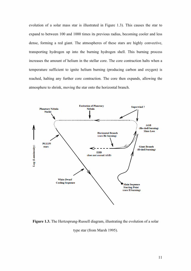
evolution of a solar mass star is illustrated in Figure 1.3). This causes the star to
expand to between 100 and 1000 times its previous radius, becoming cooler and less
dense, forming a red giant. The atmospheres of these stars are highly convective,
transporting hydrogen up into the burning hydrogen shell. This burning process
increases the amount of helium in the stellar core. The core contraction halts when a
temperature sufficient to ignite helium burning (producing carbon and oxygen) is
reached, halting any further core contraction. The core then expands, allowing the
atmosphere to shrink, moving the star onto the horizontal branch.
Figure 1.3. The Hertzsprung-Russell diagram, illustrating the evolution of a solar
type star (from Marsh 1995).
12
The burning of helium can begin before the core contraction of stars with
higher masses (2–8 M!
). In this case, since no contraction has occurred, the stellar
core will not be degenerate. In lower mass stars, the core may be under high enough
pressure to be partially degenerate when the burning of helium commences. Since
degeneracy pressure is weakly dependent on temperature, the core does not expand.
Degenerate material is a very good conductor of heat, allowing a runaway burning to
take place over only a few seconds, during which the energy production of the star
can increase by a factor of up to 1011; the helium flash. This occurs until the thermal
pressure is sufficient to drive the rising temperature, causing the core to expand and
the degeneracy to be lifted.
The helium in the core will eventually be exhausted, at which point a helium
shell will burn around a carbon/oxygen core (produced via the alpha burning process).
Again, the atmosphere expands and the star moves up the Asymptotic Giant Branch
(AGB) and onto the Red Giant Branch (RGB). The most massive stars can contain
cores of oxygen and neon (nothing heavier can be produced in stars with initial
masses < 8 M!
), surrounded by shells of progressively lighter elements, all burning to
produce progressively heavier elements. Eventually, though, this stage of the star’s
life will end. Thermal pulsations begin, ejecting the outer atmosphere of the star; for
reasons not yet clear, a superwind phase may occur toward the end of this mass loss
phase. The mass lost forms an expanding planetary nebula (PN) around the star, with
the stellar core at the nucleus. Renzini & Voli (1981) estimate that Red Giant mass
loss rates of at least 10–5 M!
yr–1 are required to account for PN observations. The
exact details of post-AGB mass loss remain poorly understood.

13
The stellar core at the centre of the expanding PN continues to contract, until
again this contraction is halted by degeneracy pressure. Over the course of this
process, the star’s Teff will increase to over 100,000 K and the log g will rise by over
four orders of magnitude. At a Teff ~ 30,000 K the UV photons emitted by the stellar
remnant will ionise the particles in the nebula. As electrons fall back to lower energy
states visible photons are emitted, giving rise to the glowing rings often seen at PN
(e.g. Figure 1.4). Eventually, the remnant PN dissipates into the ISM, the hydrogen
and helium shells stop burning, and the star becomes a young, hot white dwarf.
Figure 1.4. The Helix Nebula (NGC 7293), with the white dwarf WD 2226–210 at its
centre. Image credit: NASA, WIYN, NOAO, ESA, Hubble Helix Nebula Team, M.
Meixner (STScI) & T.A. Rector (NRAO).
1.6. White dwarf evolution.
As white dwarfs age, their evolution follows a relatively simple cooling
sequence over a timescale of the order of 109 years (this is, of course, ignoring any
14
binary interaction). However, several complications arise, giving rise to the complex
white dwarf classification system described in Table 1.1.
A carbon-oxygen core with a helium envelope, and in ~80% of white dwarfs a
hydrogen layer, is predicted by stellar evolution theory. The evolution of hydrogen
dominated DA stars is fairly straightforward. Above 50,000 K, DA white dwarfs have
a significant radiation field, which acts to levitate the metals present in the star from
either stellar nucleosynthesis or the nebula in which the star formed (if metals heavier
than those that could have been produced earlier in the star’s life are observed they
must have been produced by an earlier generation of more massive stars) into the
atmosphere, providing the photospheric metals observed at so many hot DAs (Chayer
et al. 1994, 1995a,b). Below 50,000 K the effect of radiative levitation becomes
greatly diminished, until at around 20,000 K gravitational diffusion becomes
dominant (e.g. Koester & Wilken, 2006). At a Teff ~14,000 K convection sets in (e.g.
Bergeron et al. 1995, and references therein), though in most stars the convection
zone is too shallow to dredge up significant enough amounts of helium and carbon to
pollute the photosphere.
The evolution of helium rich objects is somewhat more complex. In a late
helium flash at the end of the AGB phase, these objects are thought to lose the
majority of their hydrogen. As the star cools and contracts, the carbon and oxygen
sink out of the atmosphere, and a hot DO star is formed. Once this cools to
~45,000 K, some residual hydrogen is thought to emerge, turning the star into a DA
with a thin hydrogen layer. This is used to explain the DB gap described in Section
1.4 (though, as noted in Table 1.1, objects are now being found inside the DB gap;

15
Kleinman et al. 2004). At the cooler end of this gap (~30,000 K), helium is dredged
up, allowing the star to evolve into a DBA, then DB star.
At ~13,000 K a convection zone develops in DB stars, dredging carbon back up
into the atmosphere to form a DQ white dwarf (Pelletier et al. 1986), with a carbon
abundance peak predicted ~10,000 K (Fontaine & Brassard, 2005). Hot DQ white
dwarfs (18,000 K < Teff < 24,000 K) have been the subject of much recent study,
though their origin and evolution is not yet clear (Dufour et al. 2007a,b; 2008).
Eventually all white dwarfs will cool to a point at which no spectral features can
be seen at optical wavelengths. Thus, both hydrogen and helium rich white dwarfs
end their lives as DC stars. When the star has eventually radiated away all of its
residual heat, it will become a black dwarf (no black dwarfs have yet been observed,
since the timescale required for this process to take place is longer than the current
age of the Galaxy).
1.7. Metals in DA spectra.
Though white dwarfs are traditionally thought of as having pristine spectra, they
often display signs of metals in their atmospheres. Two processes contribute to this
metallic atmosphere content: radiative levitation and accretion (though convection can
be influential at low Teff). This section will outline these processes, and discuss in
more detail specific problems in our understanding of these mechanisms. Given the
variety of hot white dwarfs and phenomena discussed in the proceeding sections of
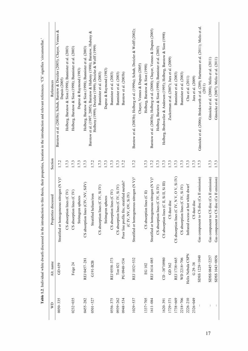
this introduction a table (Table 1.2) is given, detailing the stars explicitly discussed,
the context in which they are mentioned, the introduction section in which that

16
discussion takes place and the references used. Similarly, Table 1.3 details all of the
metal absorption/emission lines discussed throughout the thesis.
1.7.1. The case of hot DA stars.
In DA white dwarfs with Teff > 50,000 K, the upward radiation pressure from
the residual heat left over from previous stages of the star’s life counters the
downward diffusion of heavy elements. This radiative pressure lends buoyancy to the
metals in the star, an effect known as radiative levitation. Initial studies by Vauclair,
Vauclair & Greenstein (1979) found that carbon, nitrogen and oxygen could levitate
through bound-bound absorption. This theory was put on a more complete, formal
footing by Chayer et al. (1994, 1995) and Chayer, Fontaine & Wesemael (1995), who
computed predicted abundances and depth dependent distributions for the most
commonly observed metals.
Observational evidence for such metal levitation in hot DA white dwarfs has
been seen for some time, both through the presence of FUV absorption features due to
metallic elements (e.g. Sion et al. 1992; Holberg, Barstow & Sion 1998; Barstow et
al. 2003b) and the blanketing of the EUV/soft X-ray continuum by iron peak elements
(e.g. Kahn et al. 1994; Koester 1989; Barstow et al. 1993).
17
Ref
eren
ces
Bar
stow
et a
l. (2
003b
); Sc
huh,
Bar
stow
& D
reiz
ler (
2005
); C
haye
r, V
enne
s &
Dup
uis (
2005
) H
olbe
rg, B
arst
ow &
Sio
n (1
998)
; Ban
nist
er e
t al.
(200
3)
Hol
berg
, Bar
stow
& S
ion
(199
8); B
anni
ster
et a
l. (2
003)
D
upre
e &
Ray
mon
d (1
983)
H
olbe
rg, B
arst
ow &
Sio
n (1
998)
; Ban
nist
er e
t al.
(200
3)
Bar
stow
et a
l. (1
997,
200
5); B
arst
ow &
Hub
eny
(199
8); B
arst
ow, H
uben
y &
H
olbe
rg (1
999)
; Dre
izle
r (19
99);
Dre
izle
r & W
olff
(199
9)
Ban
nist
er e
t al.
(200
3)
Dup
ree
& R
aym
ond
(198
3)
Ban
nist
er e
t al.
(200
3)
Ban
nist
er e
t al.
(200
3)
Bar
stow
et a
l. (2
003b
)
Bar
stow
et a
l. (2
003b
); H
olbe
rg e
t al.
(199
9a);
Schu
h, D
reiz
ler &
Wol
ff (2
002)
; C
haye
r, V
enne
s & D
upui
s (20
05)
Hol
berg
, Bar
stow
& S
ion
(199
8)
Bar
stow
et a
l. (2
003b
); H
olbe
rg e
t al.
(200
0); C
haye
r, V
enne
s & D
upui
s (20
05)
Hol
berg
, Bar
stow
& S
ion
(199
8); B
anni
ster
et a
l. (2
003)
H
olbe
rg, B
ruhw
eile
r & A
nder
son
(199
5); H
olbe
rg, B
arst
ow &
Sio
n (1
998)
Zu
cker
man
et a
l. (2
007)
; Jur
a et
al.
(200
9)
Ban
nist
er e
t al.
(200
3)
Ban
nist
er e
t al.
(200
3)
Chu
et a
l. (2
011)
Ju
ra e
t al.
(200
9)
Gän
sick
e et
al.
(200
6); B
rinkw
orth
et a
l. (2
09);
Har
tman
n et
al.
(201
1); M
elis
et a
l. (2
011)
G
änsi
cke
et a
l. (2
008)
; Mel
is e
t al.
(201
1)
Gän
sick
e et
al.
(200
7); M
elis
et a
l. (2
011)
Sect
ion
1.7.
2
1.7.
3 1.
7.3
1.7.
3 1.
7.3
1.7.
2
1.7.
3 1.
7.3
1.7.
3 1.
7.3
1.7.
2 1.
7.2
1.7.
3 1.
7.2
1.7.
3 1.
7.3
1.7.
3 1.
7.3
1.7.
3 1.
7.3
1.7.
3 1.
7.3
1.7.
3 1.
7.3
Prop
ertie
s dis
cuss
ed
Stra
tifie
d or
hom
ogen
eous
nitr
ogen
(N V
)?
CS
abso
rptio
n lin
es (C
IV)
CS
abso
rptio
n lin
es (C
IV)
Strö
mgr
en sp
here
s C
S ab
sorp
tion
lines
(CIV
, NV
, SiIV
)
Stra
tifie
d he
lium
/iron
CS
abso
rptio
n lin
es (C
IV, S
i IV
) St
röm
gren
sphe
res
CS
abso
rptio
n lin
es (C
IV)
CS
abso
rptio
n lin
es (C
IV, S
i IV
) Po
or li
ne p
rofil
e fit
s; st
ratif
ied
met
als?
(C
IV, N
V, O
V, S
i IV
) St
ratif
ied
or h
omog
eneo
us n
itrog
en (N
V)?
C
S ab
sorp
tion
lines
(C II
) St
ratif
ied
or h
omog
eneo
us n
itrog
en (N
V)?
C
S ab
sorp
tion
lines
(C IV
, Si I
V)
CS
abso
rptio
n lin
es (C
II, S
i II,
Si II
I)
CS
dust
dis
c C
S ab
sorp
tion
lines
(C IV
, N V
, O V
, Si I
V)
CS
abso
rptio
n lin
es (C
IV, S
i IV
) In
frar
ed e
xces
s at h
ot w
hite
dw
arf
CS
dust
dis
c G
as c
ompo
nent
to C
S di
sc (C
a II
em
issi
on)
G
as c
ompo
nent
to C
S di
sc (C
a II
em
issi
on)
Gas
com
pone
nt to
CS
disc
(Ca
II e
mis
sion
)
Alt.
nam
e
GD
659
Feig
e 24
REJ
045
7–28
1
G19
1-B
2B
R
EJ 0
558–
373
Ton
021
PG 0
948+
534
R
EJ 1
032+
532
EG
102
R
EJ 1
614–
085
C
D –
38o 10
980
GD
362
R
EJ 1
738+
665
WD
221
8+70
6 H
elix
Neb
ula
CSP
N
G 2
9–38
SD
SS 1
228+
1040
SD
SS 0
845+
2257
SD
SS 1
043+
0856
Tab
le 1
.2. I
ndiv
idua
l whi
te d
war
fs d
iscu
ssed
in th
e in
trodu
ctio
n to
this
thes
is, t
heir
prop
ertie
s, lo
catio
n in
the
intro
duct
ion
and
rele
vant
refe
renc
es. ‘
CS’
sign
ifies
‘circ
umst
ella
r.’
WD
0050
–335
0232
+035
0455
–282
0501
+527
05
56–3
75
0939
+262
09
48+5
34
10
29+5
37
13
37+7
05
1611
–084
1620
–391
17
29+3
71
1738
+669
22
18+7
06
2226
–210
23
26+0
49
– – –

18
Table 1.3. The metal absorption/emission lines discussed in throughout this thesis,
with their laboratory wavelengths (in Å). Included are the low ion absorption features
that are used to characterise the ISM in Chapter 5. The features are grouped according
to their origin. All wavelengths are taken from the Kurucz database1.
Photospheric high ion absorption lines
C IV 1548.187, 1550.72
N V 1238.821, 1242.804
O V 1371.296
O VI 1031.912, 1037.613
Si IV 1393.755, 1402.770
Circumstellar high ion absorption lines
C IV 1548.187, 1550.72
N V 1238.821, 1242.804
O V 1371.296
O VI 1031.912, 1037.613
Si IV 1393.755, 1402.770
Circumstellar metal emission lines
Ca II 8500 – 8660 triplet
Fe II 5020, 5170
ISM low ion absorption lines
O I 1302.168
Si II 1260.422, 1304.370, 1526.707
S II 1259.519
Fe II 1608.536
A common technique used to measure the Teff (and log g) of a white dwarf is to
compare the observed Balmer line profiles to those predicted by model calculations
(e.g. Holberg et al. 1985; Bergeron, Saffer & Liebert 1992). As first suggested by
1http://www.pmp.uni-hannover.de/cgi-bin/ssi/test/kurucz/sekur.html

19
Dreizler & Werner (1993), line blanketing by photospheric metals significantly
affects Teff measurements for Teff > 55,000K (Barstow et al. 1998). Barstow et al.
(2001, 2003a) also found that a significant difference between the Teff values derived
from Balmer and Lyman line analyses emerges in DAs with Teff > 50,000K; a similar,
more severe effect is seen in DAO stars (Good et al. 2004). Accurate measurements
of parameters such as a white dwarf Teff are key to understanding stellar evolution;
this gives how far along the white dwarf cooling sequence the star has travelled.
Using these parameters as inputs to white dwarf evolutionary models (such as those of
Wood 1995) can allow the age and mass of the star to be calculated. Reliable
measurements of Teff are thus crucial to our understanding of white dwarf stars, and
the application of this knowledge to stellar evolution and wider astronomy.
Further complications arise when examining the patterns in metal abundances.
In their 2003 study, Barstow et al. (2003b) found that while the broad patterns
predicted between abundance and Teff and log g are reproduced, the precise
abundance predictions are often not matched by the observed values. Furthermore, in
some cases, stars with similar Teff and log g values have quite different metal
abundances. Given the importance of a proper understanding of metals in white
dwarfs to our understanding of stellar evolution, a better understanding of the
distribution of metals in hot white dwarf photospheres is therefore desirable.
1.7.2. The stratification of metals in hot DAs.
A simplifying assumption often made when modelling white dwarfs is that
their atmospheres are homogeneous. However, for many hot white dwarfs this

20
assumption conflicts strongly with observations. Indeed, radiative levitation
calculations predict a varying metal abundance with depth (e.g. Chayer, Fontaine &
Wesemael, 1995), and for the past three decades stratified atmospheres have been
used to explain some white dwarf observations.
Vennes et al. (1988) showed that radiative levitation is not as efficient at
lending buoyancy to helium when compared to carbon, nitrogen, oxygen, silicon, iron
or nickel. This causes the helium to sink though the atmosphere to leave a polluted
hydrogen layer above a helium envelope. Using similarly stratified models of
G191-B2B (WD 0501+527) with homogeneously distributed metals, Barstow &
Hubeny (1998) were able to reproduce the absence of the photospheric He II 1640 Å
line and obtain a more typical interstellar helium ionisation fraction (since the helium
observed along a given line of sight to a star is the sum of that observed in the
photosphere and that in the ISM); when fit with a homogeneous model, the interstellar
helium ionisation fraction was around 80 (±20) %, while a fraction of ~27 % was
more representative of the local ISM (LISM; Barstow et al. 1997). The stratified
models yielded a much lower ionisation fraction of 59 %, with the lower bound of
possible ionisation fraction values at 37 % nearer values reported along other lines of
sight (Barstow et al. 1997). However, a thicker hydrogen layer was required, heavily
absorbing the EUV continuum in the model and giving a poor match to the data. The
analysis of high resolution (R = 4,000) narrow band (226 Å – 246 Å) EUV data from
the Joint Astrophysical Plasma-dynamic Experiment (J-PEX) showed a better fit was
obtained with a homogeneous model (Barstow et al. 2005), in conflict with the
conclusion of Barstow & Hubeny (1998). This was attributed to either a deficiency in
the atomic data and/or a dual component, high ionisation fraction of He II along the
21
line of sight, of which one component was consistent with measurements along other
lines of sight.
The stratification of metals is also important in white dwarf atmosphere
modelling. In another investigation of WD 0501+527, Barstow, Hubeny & Holberg
(1999) found the star to have a stratified iron abundance. Here, the atmosphere was
split into a series of horizontal, homogeneous slabs with an increasing iron abundance
with depth. This model successfully explained the observed optical, FUV and EUV
observations, with a high ISM ionisation fraction of He II (in keeping with the ISM
later observed by Barstow et al. 2005). Radiatively driven mass loss was used to
explain iron depletion in the upper atmosphere. Dreizler (1999) and Dreizler & Wolff
(1999) also constructed stratified models to study the EUV spectrum of WD
0501+527, using depth dependent radiation intensity, and the chemical abundances at
each depth point were those produced by the equilibrium of radiative levitation and
downward diffusion. This method successfully modelled the EUV spectrum of WD
0501+527 without the interstellar He II column density detected, at odds with the
interstellar measurements of Barstow & Hubeny (1998), Barstow, Hubeny & Holberg
(1999) and Barstow et al. (2005).
Observations of metals other than iron have required stratified chemical
configurations. Nitrogen stratification was used to explain the observed line profiles
of the FUV N V doublet (1238.82 Å, 1242.80 Å) in the 44,350±715 K DA REJ
1032+532 (WD 1029+537; Barstow et al. 2003b, Holberg et al. 1999a). A
homogeneous nitrogen distribution with a log(N/H) of –4.31 gave a line profile with a
depth similar to that observed. However, such a high nitrogen abundance in the lower

22
atmosphere caused the model absorption features to be heavily pressure broadened
beyond the observed line profile. A thin nitrogen layer at the top of the atmosphere
(!M/M = 3.1x10⁻¹⁶) reproduced the observed line profiles well; the high nitrogen
abundance provided the deep line profile, while not having nitrogen lower in the
atmosphere avoided such heavy pressure broadening (Figure 1.5).
Holberg et al. (1999a) also considered the EUV spectrum of WD 1029+537
(Figure 1.6). The presence of nitrogen at high abundance in the lower atmospheric
region of the homogeneous model causes significant EUV absorption, due to both
nitrogen absorption edges at 180 and 260 Å and absorption lines at specific
wavelength above 135 Å (Figure 1.6, lower curve). The stratified nitrogen removes
this EUV absorber, better matching the data (Figure 1.6, upper curve). It was
concluded that, given the stratified nitrogen distribution matched both the FUV N V
line profiles and the EUV continuum, the star had a slab of high abundance nitrogen
at the top of its atmosphere. This distribution was again put down to a radiatively
driven mass loss process, which enigmatically affected only nitrogen (the carbon and
silicon in this star were well modelled using a homogeneous distribution).
A similar nitrogen configuration has been suggested for GD 659 (WD 0050–
332; Teff = 35,660±135 K, Barstow et al. 2003b), which displays a pure hydrogen
EUV spectrum with FUV carbon, nitrogen and silicon absorption features (Barstow et
al. 2003b). REJ 1614–085 (WD 1611–084; 38 840±480 K, Barstow et al. 2003b) has
also been examined in this context, and was found to have strong N V FUV
absorption lines, again indicative of a slab of nitrogen in the higher atmospheric
region (Holberg et al. 2000; Barstow et al. 2003b).

23
Figure 1.5. The N V resonance doublet of WD 1029+537 (Figure 5, Holberg et al.
1999a). A layer of nitrogen (log(N/H) = –4.31) in the topmost part of the atmosphere
("M/M = 3.1x10⁻¹⁶) is illustrated with the upper curve. A homogeneous nitrogen
distribution is shown with the lower curve.

24
Figure 1.6. The EUVE spectrum of WD 1029+537 (Figure 6, Holberg et al. 1999a).
The homogeneous model is again shown by the lower curve and the stratified nitrogen
configuration is indicated with the upper curve.
When examining the patterns in the metal abundances of hot DA white
dwarfs, WD 1029+537, WD 1611–084 and WD 0050–332 stand out as interesting
objects. Barstow et al. (2003b) find no correlation between nitrogen abundance and
Teff, for stars with Teff > 50,000 K. Below 50,000 K, heavy elements should begin to
sink out of the atmosphere due to the reduced dominance of radiative levitation.
However, a dichotomy is observed. WD 1029+537, WD 1611–084 and WD 0050–
332 show an increase in nitrogen abundance with decreasing Teff, while all other white
dwarfs show no nitrogen and only upper limits can be estimated (Figure 1.7), hinting
that these three objects may in some way be special.

25
Figure 1.7. Measured nitrogen abundance as a function of Teff (Figure 10, Barstow et
al. 2003b). WD 1029+537, WD 1611–084 and WD 0050–332 are the three objects
with Teff < 50,000 K with nitrogen detections.
Schuh, Dreizler & Wolff (2002) used stratified model sets of the type of
Dreizler (1999) and Dreizler & Wolff (1999) to model the EUVE spectra of a sample
of DA white dwarfs, and explained the EUV properties of many of their objects well.
However, four DAs (WD 1314+293, WD 1029+537, WD 2004–605 and WD 2152–
548) were better represented by homogeneous models (the WD 1029+537 result being
in direct conflict with that of Holberg et al. 1998a and Barstow et al. 2003b). Four
other white dwarfs (WD 0027–636, WD 1056+516, WD 1234+481 and WD
2111+498) were not well fit; this was interpreted as accretion disturbing the radiative
levitation/downward diffusion balance. Furthermore, a comparison by Schuh,
Barstow & Dreizler (2005) of the abundance patterns measured using the stratified
models of Schuh, Dreizler & Wolff (2002) to those measured by Barstow et al.

26
(2003b) found the nitrogen abundances of WD 0050–332, WD 1029+537 and WD
1611–084 were in keeping with the other white dwarfs of higher Teff (Figure 1.8), in
stark conflict with the results of Barstow et al. (2003b). Oxygen abundances were
roughly consistent. The stratified C III and C IV abundances were consistently over-
predicted when compared to the homogneous models, while silicon was generally
over predicted for Teff < 50,000 K and under predicted for Teff > 50,000 K. The iron
and nickel abundances were within the systematic errors expected between both
model sets, and the Fe:Ni ratio was ~20, consistent with the cosmic value and that of
Barstow et al. (2003b).
Figure 1.8. Figure 1 from Schuh, Barstow & Dreizler 2005. A comparison of the
nitrogen abundances using the stratified models of Schuh, Dreizler & Wolff (2002;
light grey data points) to the measurements of Barstow et al. (2003b; black data
points). The radiative levitation predictions of Chayer et al. (1995) are denoted with
dark grey symbols, while the cosmic abundance is shown with the dotted line.

27
A later study of WD 0050–332, WD 1029+537 and WD 1611–084 by Chayer,
Vennes & Dupuis (2005) found that the nitrogen line profiles and EUV data could be
explained with homogeneous nitrogen distributions, with much lower abundances
(log(N/H) = –6.2, –5.2 and –5.9 for WD 1029+537, WD 1611–084 and WD 0050–
332, respectively; Figure 1.9) than those found by Barstow et al. (2003b).
Figure 1.9. Figure 1 from Chayer, Vennes & Dupuis 2005. A comparison of the
log(N/H) values found by Chayer, Vennes & Dupuis (open circles) to those found by
Barstow et al. (2003b; filled circles).
Another star to show anomalous line profiles is the extremely hot DA PG
0948+534 (WD 0948+534, Teff = 110,000±2,500 K, Barstow et al. 2003b). The C IV,
N V, O V and Si IV absorption features in the STIS data of this star are again
extremely narrow and, in the case of C IV, almost completely saturated (Figure 1.10).

28
Given the similarity between this doublet and the N V doublets in WD 1029+537,
WD 1611–084 and WD 0050–332, it was suggested by Barstow et al. (2003b) that the
carbon might be similarly distributed in a slab in the upper atmosphere. Indeed, their
preliminary calculations supported this hypothesis.
Figure 1.10. The C IV doublet in the STIS spectrum of WD 0948+534.
Given the differing conclusions of the analyses of the nitrogen abundance and
distribution in WD 1029+537, WD 0050–332 and WD 1611–084, a detailed analysis
of the nitrogen in these stars is desirable, and is described in Chapter 3. Since
stratified, high abundance models have been used to explain the metal absorption
features of WD 0948+534, the analysis is also extended to this object.

29
1.7.3. Circumstellar material at hot DA stars.
In addition to absorption features from highly ionised photospheric material,
absorption features at non-photospheric velocities have been seen in the spectra of hot
DAs during the past few decades of white dwarf research. The IUE spectrum of Feige
24 (WD 0232+035, a close binary system consisting of a hot DA white dwarf and an
M dwarf) displays two sets of C IV absorption features (e.g. Dupree & Raymond
1982). This is interpreted as one set of photospheric features, where the changing
velocity of the component reflects the orbital motion of the DA (Vennes et al. 1992),
and a set of stationary features arising in a hot circumstellar gas. Again using IUE
observations, Si II, Si III and C II absorption features are seen with a velocity far from
the photospheric and interstellar velocities at CD –38o 10980 (WD 1620–391,
Holberg, Bruhweiler & Anderson 1995), indicating the presence of a photoionised
circumstellar cloud around the star.
A survey of 55 white dwarf IUE spectra (Holberg, Barstow & Sion, 1998)
found 11 stars with evidence of circumstellar material, of which five were DAs (WD
0050–332, WD 0232+035, WD 0455–282, WD 1337+705, WD 1611–084 and WD
1620–391). These circumstellar features were all blueshifted, occupied a narrow
velocity range (40 – 60 km s–1), and were attributed to mass loss from the white
dwarfs. Lines of sight close to the white dwarfs showed no ISM absorption features
consistent with the observed circumstellar lines. Also, the ISM features seen along
such sight lines had both red and blueshifted velocities with respect to the
photosphere. In a more recent survey of 23 hot DA white dwarfs, using data from IUE
and HST STIS/GHRS, eight white dwarfs were found with circumstellar material, with

30
two further possible detections (Bannister et al. 2003). Potential sources of this
material were put forward, and included the ionisation of nearby ISM in the
‘Strömgren sphere’ of the white dwarf, material inside the gravitational well of the
star, mass loss in a stellar wind and ancient planetary nebulae (PNe). Indeed, WD
2218+706 (one of the objects exhibiting circumstellar absorption in the sample of
Bannister et al. 2003) is located within the old planetary nebula (PN) DeHt5 (e.g.
Napiwotzki & Schöberner, 1995).
In recent years, research into the circumstellar environments of white dwarfs
has yielded many interesting results. The diffusion timescales of metals in the
photospheres of cooler white dwarf stars (Teff < 25,000 K) is extremely short (e.g.
Koester & Wilken, 2006), requiring an external source of metals near the white dwarf
to maintain the observed abundances (radiative levitation has recently been found to
have some effect in these cooler white dwarfs, although accretion is still required to
explain the observed metal abundances; Chayer & Dupuis 2010; Dupuis, Chayer &
Hénault-Brunet, 2010; Dupuis et al. 2010).
Dupuis et al. (1992, 1993) and Dupuis, Fontaine & Wesmael (1993) proposed
a ‘two phase accretion model’ to explain the atmospheric pollution, where a white
dwarf would encounter an ISM cloudlet and accrete metals. After passing through the
cloudlet, the photosphere of the white dwarf would still contain observable metals
until the diffusion timescale had passed. However, studies looking at white dwarf
kinematics reported that cool, metal rich white dwarfs were sufficiently far from ISM
cloudlets for all the metals in their photospheres to have fully diffused downwards,
given their velocities and positions (e.g. Aannestad et al. 1993). Indeed, some white

31
dwarfs displaying metallic photospheres were about to move into a cloudlet, and
should not have had any metals in their photospheres. Subsequent studies
demonstrated that metals may be accreted from more local sources, such as comets,
mass lost from a binary companion (e.g. Zuckerman & Reid, 1998) or disrupted
asteroids (e.g. Zuckerman et al. 2003; Jura, 2003, 2006, 2008).
Infrared studies show evidence of circumstellar dust discs at some of the cool
DAZ stars, and the accretion of this dust introduces polluting metals to the white
dwarf photospheres (e.g. Kilic et al. 2005, 2006; Kilic & Redfield, 2007; von Hippel
et al. 2007; Farihi, Zuckerman & Becklin, 2008). A study with the Spitzer IRAC and
MIPS instruments shows that, when combined with previous work, no more than 20%
of all single white dwarfs with an implied metal accretion rate > 3x10⁸ g s–1 display
infrared emission from a dust disc (Farihi, Jura & Zuckerman, 2009). It is reasoned
that, since this accretion rate is between the dust production rates in the Solar System
zodiacal cloud (106 g s–1) and the debris discs around main-sequence A type stars
(1010 g s–1), these discs are produced by the tidal disruption of extrasolar minor
planets and/or asteroids, an idea first put forward by Graham et al. (1990) and
developed by Debes & Sigurdsson (2002). Silicate emission from circumstellar dust
at six externally polluted white dwarfs adds weight to this model (Jura, Farihi &
Zuckerman, 2009). Farihi et al. (2010) report no relation between the accreted
calcium abundances and the presence of clouds in the ISM for 146 DZ Sloan Digital
Sky Survey (SDSS) white dwarf spectra. It was also found that for Teff < 12,000 K,
the DBZ and DC white dwarfs belonged to the same stellar populations, implying that
the metal pollution in the DBZ stars must be from tidally disrupted rocky planets
since ISM accretion would also be evident in the DC stars.
32
The relative metal abundances of the DB GD 362 (9,850±100 K) show that
the white dwarf is likely to be accreting from a large, disrupted asteroid/asteroids with
an Earth-Moon composition (Zuckerman et al. 2007). An infrared and X-ray analysis
reports evidence for the accretion of either 100 Ceres-like asteroids or one large
object by both GD 362 (given the anomalously large relative amount of hydrogen in
the material accreted by this star) and G29–38 (Jura et al. 2009). An alternative
scenario is that a single parent body with a mass between that of Callisto and Mars,
containing internal water, has been disrupted and is being accreted. Further studies
have found many other white dwarfs harbouring the remains of extrasolar planets
(e.g. Dufour et al. 2010; Klein et al. 2011; Melis et al. 2011; Zuckerman et al. 2011).
Gaseous components have been found at some white dwarf circumstellar
discs. The optical spectrum of SDSS J122859.93+104032.9 (Teff = 22,020 K,
hereafter SDSS J1228+1040) displays emission from the Ca II 8500–8660 Å triplet
(Figure 1.11, right hand panel), as well as weaker emission from Fe II at 5020 and
5170 Å (Gänsicke et al. 2006). The star also exhibits photospheric Mg II absorption
(4482 Å, Figure 1.11, left hand panel), with roughly a solar abundance, suggesting a
metal rich disc. The lack of photospheric He I absorption at 4470 Å (providing an
abundance upper limit of 0.1 times the solar abundance) or Balmer and helium
emission from the disc, lends further weight to the metallic composition of the
circumstellar disc. The asymmetry in the double peaked Ca II emission line is
indicative of an asymmetric disc, with an estimated outer disc radius of 1.2 R!
,
comparable to the tidal disruption radius for a rocky asteroid (Davidsson, 1999). Time
resolved spectroscopy and photometry do not reveal any radial velocity variations,
33
showing no detectable interacting binary companion is present from which material
could be accreted.
Detailed modelling of this circumstellar gas disc at SDSS J1228+1040 shows
that the Ca II triplet emission can arise from a metallic gas disc inside the tidal
disruption radius of the star, with a disc Teff ~ 6,000 K and surface mass density of
~0.3 g cm–2 (Hartmann et al. 2011). The asymmetry in the emission is found to be due
to either a spiral arm structure or disc eccentricity. However, the models of Hartmann
et al. (2011), which assume a chemical composition typical for Solar System asteroids
(including hydrogen, carbon, nitrogen, oxygen, magnesium, silicon and calcium),
predict C II, O II, Si I, Si II, Mg I and Mg II emission that is not seen, and should
therefore be treated with caution.
As shown in Figure 1.11, Gänsicke et al. (2007, 2008) have also found
metallic gas discs around the DAZ SDSS J104341.53+085558.2 (hereafter SDSS
J1043+0856) and the DBZ SDSS J084539.17+225728.0 (hereafter SDSS
J0845+2257). GD 362 and WD 1337+705 (which has an anomalously high metal
abundance) were also examined by Gänsicke et al. (2007), although no circumstellar
gas discs were detected. Brinkworth et al. (2009) found a dust disc was also present at
SDSS J1228+1040, demonstrating for the first time a debris disc with dust and gas
components. A further study by Melis et al. (2011) found that both SDSS J1043+0856
and SDSS J0845+2257 also harbour dust discs that are spatially coincident with the
gas discs.

34
Figure 1.11. Figure 1 from Gänsicke et al., 2008. The left hand panel shows the
photospheric Mg II (4481 Å) absorption lines in the William Herschel Telescope
(WHT) spectra of WD1337+705, SDSS 1228 and SDSS 1043 (black lines), with the
best fitting white dwarf models (grey). The right panel shows the 8350–8800 Å region
of the spectra of WD 1337+705, GD 362, SDSS 1228 and SDSS 1043, normalised
and offset for clarity. WHT spectra are shown in black, while the SDSS spectra are
plotted in grey.

35
An infrared excess is seen at the central star of the helix nebula (Su et al.
2007), which may be due to a circumstellar disc. Unlike the circumstellar discs
prevalent at cooler white dwarfs, these dust discs are around 30 – 150 AU from the
central star of the PN (CSPN). In a recently published survey of 71 hot white dwarfs,
with 35 CSPNe, Chu et al. (2011) report that ~20 % of the surveyed stars have
infrared excesses. Only 5–6 % of non-PN stars have similar infrared excesses. While
a Kuiper belt type dust disc has been put forward as a source for the infrared
emission, it must be stressed that the exact origin of these infrared excesses is not
fully understood, and could also be due to PN material or binary companions. A
recent publication on the WIRED survey suggests that four of the DAs in the survey
with Teff > 30,000 K have infrared excesses that could be due to circumstellar discs,
although the observations may suffer from contamination from background objects
(Debes et al. 2011).
In addition to circumstellar discs being a possible source of the circumstellar
high ions, the ionisation of ISM material near to the star may provide a source of the
shifted absorption components. Previous studies have attempted to quantify this
effect. Dupree & Raymond (1983) looked to white dwarf Strömgren spheres to
explain the high ion absorption features seen in the spectra of WD 0232+035 (Feige
24) and WD 0501+527 (G191-B2B), although these absorption features have since
been found to originate in the photospheres of the stars (except the circumstellar C IV
lines seen at these DAs). In an examination of the UV ionisation of the local ISM
(LISM) within 20 pc of the Sun, Tat & Terzian (1999) concluded that material inside
the Strömgren spheres of nearby white dwarfs could be responsible for the observed
LISM ionisation. Of the 121 stars studied, 24 had Strömgren radii (rS) > 0.5 pc. Since
36
only stars within 20 pc were considered, the significant effect of B stars within 100 pc
(Vallegra, 1999) was ignored, as was the presence of the rarefied “tunnel” towards !
CMa (Welsh, 1991) and the local chimney (Welsh et al. 1999). Welsh et al. (2010a)
observed a series of cell-like cavities in their 3-D maps of the LISM (out to 300 pc),
attributed to the ionisation of the ISM near B stars and some hot white dwarfs. The
evaporation and photoionisation of circumstellar material by the radiation field of hot
white dwarfs was used to explain the circumstellar high ion absorption features seen
in the spectra of the three stars studied by Lallement et al. (2011).
A proper understanding of the origin of the circumstellar absorption seen at
hot white dwarfs is crucial. Should, as highlighted by Lallement et al. (2011), the non-
photospheric O VI attributed to the ISM by Savage & Lehner (2006) and Barstow et
al. (2010) in fact be photoionised material local to the white dwarfs, then erroneous
interpretations of the physical state of the LISM may have been made. This could
explain the confused view of local hot interstellar gas. Indeed, Lallement et al. (2011)
found evidence that suggests hot/cold gas interfaces cannot give rise to the observed
non-photospheric features. This echoes the finding of Welsh et al. (2010a,b), that the
Doppler widths of the observed non-photospheric high ion absorption features are
inconsistent with hot/cold gas interfaces, and better suit photoionisation by B stars
and hot white dwarfs. This shows a clear need to understand the true nature of the
non-photospheric high ions seen in the spectra of hot DA white dwarfs.

37
1.8. Modelling white dwarf stars.
The white dwarf atmosphere models used in this work were constructed using
the TLUSTY program (e.g. Hubeny & Lanz 1992, 1995, 2003; Hubeny, Hummer &
Lanz, 1994; Lanz & Hubeny 1995, 2003a,b). Spectra were synthesised using the
accompanying SYNSPEC code. Although the precise computational techniques used
to construct stellar atmospheres vary, and an exhaustively detailed account of the
programs used is not given here, the basic physical principles are discussed.
The model atmosphere is assumed to be plane parallel and horizontally
homogeneous. The incoming flux from the stellar core is fixed by the model Teff, and
TLUSTY solves the hydrostatic, ionisation and excitation equilibrium in each of these
atmospheric layers in the presence of specified chemical abundances. The results of
these calculations provide the density, temperature, mass, electron density, log g,
Rossland optical depth and flux at each depth point, along with details of the
ionisation and excitation balance, which are then used to calculate the opacity in each
layer due to each transition detailed during spectrum synthesis with SYNSPEC. The
model ions used here are those constructed for the TLUSTY code2, which contain the
individual energy levels/super levels, oscillator strengths and photo-ionisation cross
sections of each ion. These ionic data come from the Opacity Project TOPBASE3
database. Significant variety can be found in the values of such data, depending on the
source of the data (e.g. whether the data is taken from the TOPBASE database, the
2 http://nova.astro.umd.edu/Tlusty2002/tlusty-frames-data.html 3 http://cdsweb.u-strasbg.fr/topbase/topbase.html

38
NIST Atomic Spectra Database4, etc), and uncertainties in quantities such as the
oscillator strengths (i.e. the probability of a give transition occurring) may have a
significant impact on the atmosphere calculation and synthesised spectrum. Similarly,
grouping energy levels into either into a “superlevel” (where a closely spaced of
discrete energy states are approximated to one level to reduce the complexity of the
model ion) may impact upon the calculated model in the high Teff regime where high
ions of the complex iron peak elements are present. For iron peak elements, each
model ion requires four files, one containing the model atom (with the superlevels,
line transitions and energy limits), one with the photoionisation cross sections, a file
with the Kurucz level data and another with the Kurucz line data, to allow the proper
inclusion of line blanketing effects.
Many atmosphere calculations assume local thermodynamic equilibrium (LTE),
where the gas is collisionally ionised, the thermodynamic variables of the system
obey their classical relations, and the system is in ionisation equilibrium. Such an
approximation considerably lightens the computational burden of the model
calculation, and is an appropriate approximation for cooler stars. However, in hot
white dwarfs, radiative ionisation is the dominant process. A series of studies in the
mid-1990s (e.g. Lanz & Hubeny 1995; Lanz et al. 1996; Napiwotzki 1997) found that
inclusion of non-LTE (NLTE) effects have the most significant effect on Teff
measurements, more so than the inclusion of photospheric metals. These NLTE
effects can easily be incorporated into model calculations using the TLUSTY
program.
4 http://physics.nist.gov/PhysRefData/ASD/lines_form.html

39
As already alluded to in Section 1.7.1, a white dwarf’s Teff and log g can be
measured using models of the Balmer/Lyman line profiles. The strength of the
absorption lines decrease as Teff increases, since more hydrogen atoms become
ionised, leaving progressively less electrons in the n=2 state. Analogously, the line
profile broadens as log g increases, since density increases. This allows the energy
level of each atom to be affected by its neighbouring ions and electrons, creating
perturbations of the energy level structure that broaden the absorption feature, and the
higher the density the more severe this effect. Grids of models are produced, with
varying Teff and log g values, which are compared to the observed data. The
parameters of the model that best matches the observed data are adopted as those of
the observed star.
Analogously, to measure metal abundances, grids of models are calculated with
varying metal abundances. The metal abundance of the model that best reproduces the
observed metal absorption line profiles (found at FUV and EUV wavelengths) is
adopted as the metal abundance present in the star. The model fitting in this work
was achieved using the XSPEC package (Arnaud, 1996), which utilised a
!
"#2
minimisation technique based on a modified Levenberg-Marquardt algorithm.
1.9. Structure of thesis.
This thesis is split into six chapters. The proceeding chapter details the
instruments used in this work. Chapter 3 examines the stratification of metals
(particularly nitrogen) in some anomalous DA stars. Chapter 4 describes a search for
circumstellar gas discs at a sample of hot DAs, while Chapter 5 presents a study of the

40
origin of circumstellar absorption features in hot DA white dwarfs. Chapter 6 contains
some concluding remarks and suggests the direction of future investigations in this
field.
1.10. Summary.
• White dwarfs are the evolutionary end point of the vast majority of stars. They
are compact objects (7 < log g < 9), with degenerate cores, mainly hydrogen
or helium dominated atmospheres, and are classified by their spectral
characteristics.
• Metals are present in the photospheres of hot white dwarfs due to radiative
levitation (and in some cases accretion). However, the metal abundances
observed in hot white dwarfs are often not consistent with those predicted with
radiative levitation theory. Some stars of similar Teff exhibit quite varied metal
abundances, and some uncertainty exists in the distribution of metals in some
stars. A thorough understanding of the abundance and distribution of metals in
DAs with anomalous abundance measurements is desirable.
• Metal pollution from circumstellar discs is responsible for the photospheric
metals seen in cooler white dwarfs where radiative levitation does not
dominate the DA atmosphere. It is becoming widely accepted that these discs
form via the tidal disruption of asteroids and minor planetary bodies in Solar
System analogues. Gaseous components have also been detected at some
discs, thought to be from vigorous collisions between dust particles. Searching

41
for gas discs at hot DAs is an important task, since such discs could provide a
polluting mechanism to account for the observed abundance anomalies.
• Non-photospheric metal absorption features are seen at some hot DA white
dwarfs. Sources put forward for these features have been material in the
potential wells of the stars, the ionisation of the ISM local to the stars, stellar
mass loss and ancient PNe. A proper understanding of the origin of these non-
photospheric absorption features is required to better understand the hot white
dwarf circumstellar environment and the interaction of hot white dwarfs with
the ISM in their locality.

42
Chapter 2.
Instruments used and white dwarf studied.
2.1. Introduction.
The instruments used to obtain the data studied in this thesis are outlined here.
These include the Space Telescope Imaging Spectrograph (STIS) and Goddard High
Resolution Spectrometer (GHRS) aboard the Hubble Space Telescope (HST), the
International Ultraviolet Explorer (IUE), the Extreme Ultraviolet Explorer (EUVE),
the Far Ultraviolet Explorer (FUSE) and the Intermediate dispersion Spectrograph
and Imaging System (ISIS), at the William Herschel Telescope (WHT). Following
these is a subsection detailing all of the stars studied in this thesis.
2.2. The Space Telescope Imaging Spectrograph (STIS).
STIS replaced the Faint Object Spectrograph (FOS), and was installed on the
HST in 1997 during the second servicing mission by the astronauts Mark Lee and
Steven Smith. In 2004 a fault developed in a circuit board, ending STIS’s use for some
five years. The fourth servicing mission saw Michael Good and Mike Massimino
replace the faulty part on 17th May 2009, after which the instrument performed almost

43
as expected, when CCD radiation damage and changes in throughput during STIS’s
downtime were taken into account.
Three detectors are present on STIS. The CCD has ~0.05 arcsecond square
pixels, with a field of view (FOV) 52x52 arcsecond squared, and covers
2,000 – 10,300 Å. The near ultraviolet (NUV) Cs2Te Multi-Anode Microchannel
Array (MAMA) covers 1,600 – 3,100 Å, and has ~0.024 arcsecond square pixels with
a 25x25 arcsecond square FOV. The third detector, the far ultraviolet (FUV) solar-
blind CsI MAMA (FUV-MAMA), has the same FOV and pixel size as the NUV-
MAMA, but operates in the 1150 – 1700 Å range. The spectra used in this work were
taken with FUV-MAMA detector using the E140M and E140H gratings, providing
resolving powers of 40,000 and 110,000. The design and on-orbit performance of
STIS are detailed by Woodgate et al. (1998) and Kimble et al. (1998).
2.3. The Goddard High Resolution Spectrograph (GHRS).
Replaced by the Near Infrared Camera and Multi-Object Spectrometer
(NICMOS) during the second servicing mission in 1997, the Goddard High
Resolution Spectrograph (GHRS) was one of HST’s original instruments. GHRS
observed from 1150 – 3200 Å. The data used here were taken in the G160M mode,
with a resolving power of 22,000.

44
2.4. Intermediate dispersion Spectrograph and Imaging
System (ISIS).
Mounted on the 4.2m William Herschel Telescope (WHT), at the Isaac
Newtown Group (ING) of Telescopes on La Palma, the Intermediate dispersion
Spectrograph and Imaging System (ISIS) offers single slit spectroscopy over the
3,000 – 100,000 Å wavelength range. The R1200 grating was used in the observations
carried out for the work in this thesis. With a central wavelength of 4899 Å, the blue
arm observations (with the EEV12 chip) have a specific central wavelength resolution
of 0.224 Å. The observations making use of the red arm of the spectrograph (the
Red+ chip) have a specific central wavelength resolution of 2.41 Å for a central
wavelength of 8600 Å.
2.5 The Far Ultraviolet Spectroscopic Explorer (FUSE).
The Far Ultraviolet Spectroscopic Explorer (FUSE), launched on 24th June
1999, operated until 18th October 2007. A detailed overview of the mission can be
found in Moos et al. (2000), and the on-orbit performance of the observatory was
reported by Sahnow et al. (2000).
Four co-aligned, prime focus telescopes and Rowland spectrographs with
microchannel plate (MCP) detectors provided wavelength coverage from
905 – 1187 Å. Two telescope channels were coated with SiC to optimise the
905 – 1105 Å throughput and the channels covering 1000 – 1187 Å were covered

45
with Al:LiF to optimise reflectivity. According to Sahnow et al. (2000), the velocity
resolutions were ~17 km s–1 in the 905 – 1105 Å region and ~13 km s–1 in the
1000 – 1187 Å region.
Point source spectra often displayed a depression in flux, most noticeably
spanning up to 50 Å of the LiF channel 1, detector segment B (1BLiF) spectra taken
with the low resolution aperture (LWRS), caused by the shadow of the quantum
efficiency (QE) grid wires. Given the time variability of these features (even within
individual space craft orbits), they were termed ‘worms’, with the affected spectral
region called the ‘region of the worm’ (Figure 2.1). The relationship between the
precise position and alignment of the detector’s QE grid wires, the optical elements,
telescope illumination, pointing stability, the photon’s wavelength and the
instrument’s optical design was highly complex, and the models used to calibrate for
the worm failed to fully account for the effect; the minor errors in the telescope
pointing and alignment caused the observed target to drift on the detector, causing the
shadow’s position to move, causing the worm to vary in both flux and wavelength
space.
FUSE spectra also suffered severely with airglow emission (‘sky lines’),
caused by the excitation of H I, N I, N II, and O I in the Earth’s upper atmosphere by
solar activity (Feldman et al. 2001). This effect was more significant on dayside
observations, when the observatory was orientated so that the path length of the light
observed through the Earth’s atmosphere was longer, and when the Sun was active.
Given the variability of this effect, each data set needed to be inspected to establish its
severity. In the most severe cases use of the data was limited.

46
Figure 2.1. Two WD 0501+527 FUSE spectra, showing the 'region of the worm'. The
upper panel shows the 1BLiF spectrum from observation M1010201000 (13th October
1999 01:25:31) and the lower panel is from observation M1030602000 (21st
November 1999 11:39:56).

47
2.6. The Extreme Ultraviolet Explorer (EUVE).
The Extreme Ultraviolet Explorer (EUVE) was launched on 7th June 1992,
stopped operation on 31st January 2001 and re-entered the Earth’s atmosphere on 30th
January 2002. EUVE observed in the 70 – 760 Å range, was the first dedicated EUV
mission, and consisted of four photometric imaging systems and a three channel
(short wave, SW, 70 – 190 Å; medium wave, MW, 140 – 380 Å; long wave, LW,
280 – 760 Å) spectrometer. The resolution of the three spectrometers was 0.5 Å, 1.0
Å and 2.0 Å for the SW, MW and LW channels, respectively. A complete sky survey
was undertaken using the imaging systems, with the spectrometers being used for
pointed spectroscopic observations of over 350 objects.
2.7. The International Ultraviolet Explorer (IUE).
Launched on 26th January 1978, the International Ultraviolet Explorer (IUE) is
the oldest source of data used here. Greatly exceeding its expected operational
lifetime of 3 years, IUE was finally shut down on 30th September 1996 after obtaining
over 104,000 spectra. IUE’s spectrometers covered the 1,200 – 3,350 Å wavelength
region at high (0.1 – 0.3 Å) and low (6 – 7 Å) resolutions. Two spectrographs were
present on IUE, covering a short wavelength range (SW; 1,150 – 2,000 Å) and a long
wavelength range (LW; 1,850 – 3,300 Å). Each spectrograph had two cameras, the
prime (P) camera and a redundant (R) camera, carried in case of a failure of the prime
camera. The data used here was taken in the SWP mode, with a resolving power of
20,000.

48
2.8. White dwarfs studied.
Table 2.1 details all of the white dwarfs studied in this thesis, their Teff, the
property of interest and the instruments from which the data analysed in each
investigation was obtained. Spitzer infrared observations are included that, though not
analysed here, prove useful in interpreting the results of the analyses.

49
Sour
ce(s
) of d
ata
IS
IS; S
pitz
er IR
AC*‡
H
ST S
TIS;
EU
VE
IUE;
HST
STI
S; S
pitz
er IR
AC*‡
W
HT
ISIS
H
ST S
TIS
IUE;
Spi
tzer
IRAC
*‡
HST
STI
S; S
pitz
er IR
AC*‡
H
ST S
TIS
IUE;
Spi
tzer
IRAC
*‡
HST
STI
S; S
pitz
er M
IPS**
‡ H
ST S
TIS
HST
STI
S; S
pitz
er M
IPS**
‡ H
ST S
TIS;
EU
VE
HST
STI
S H
ST G
HRS
H
ST S
TIS
IUE;
Spi
tzer
IRAC
*‡
IUE
IUE;
Spi
tzer
IRAC
*‡
HST
GH
RS
WH
T IS
IS; S
pitz
er IR
AC*‡
H
ST G
HRS
; Spi
tzer
IRAC
*‡
HST
STI
S; S
pitz
er M
IPS**
‡ W
HT
ISIS
; Spi
tzer
IRAC
*‡
WH
T IS
IS
IUE
WH
T IS
IS; S
pitz
er IR
AC*‡
IUE;
HST
GH
RS; S
pitz
er IR
AC*‡
HST
STI
S
Prop
ertie
s of i
nter
est
Circ
umst
ella
r gas
dis
c?
Stra
tifie
d ni
troge
n?
Circ
umst
ella
r hig
h io
ns?
Circ
umst
ella
r gas
dis
c?
Circ
umst
ella
r C IV
Circ
umst
ella
r C IV
, NV
, Si I
V
Circ
umst
ella
r C IV
, Si I
V
Circ
umst
ella
r C IV
C
ircum
stel
lar h
igh
ions
? C
ircum
stel
lar C
IV, S
i IV
St
ratif
ied
met
als?
C
ircum
stel
lar h
igh
ions
? St
ratif
ied
nitro
gen?
C
ircum
stel
lar h
igh
ions
? C
ircum
stel
lar h
igh
ions
? C
ircum
stel
lar h
igh
ions
? C
ircum
stel
lar h
igh
ions
? C
ircum
stel
lar h
igh
ions
? C
ircum
stel
lar h
igh
ions
? St
ratif
ied
nitro
gen?
C
ircum
stel
lar g
as d
isc?
C
ircum
stel
lar h
igh
ions
? C
ircum
stel
lar h
igh
ions
? C
ircum
stel
lar g
as d
isc?
C
ircum
stel
lar g
as d
isc?
C
ircum
stel
lar h
igh
ions
? C
ircum
stel
lar g
as d
isc?
Circ
umst
ella
r hig
h io
ns?
Circ
umst
ella
r hig
h io
ns?
Cha
pter
4 3 5 4 5 5 5 5 5 5 3 5 3 5 5 5 5 5 5 3 4 5 5 4 4 5 4 5 5
T eff (K
) 47
,219
* 35
,660
±135
36,0
00†
60,4
87±1
,100
50,9
60±1
,070
52,5
00±9
00
59,5
08±2
,200
58
,200
±1,8
00
69,7
11±5
30
110,
000±
2500
44,3
50±7
15
39
,770
±615
54
,574
±900
39
,290
±340
50
,370
±870
22
,090
±85
38,8
40±4
80
66
,760
±1,2
30
34,0
56*
19,1
50±3
0
39,2
90±3
60
45,5
00±1
,085
Alt.
nam
e G
D 2
G
D 6
59
H
S 02
09+0
83
Feig
e 24
REJ
045
7–28
1
G19
1-B
2B
REJ
055
8–37
3 R
EJ 0
623–
371
Ton
021
PG 0
948+
534
R
EJ 1
032+
532
PG
105
7+71
9 PG
112
3+18
9 G
D 1
53
HZ
43
EG 1
02
REJ
161
4–08
5
REJ
173
8+66
5 R
EJ 1
943+
50
Wol
f 134
6
GD
394
REJ
215
6–54
6
Tab
le 2
.1. T
he w
hite
dw
arfs
stud
ied
here
, the
ir st
ella
r par
amet
ers,
the
chap
ters
in w
hich
they
are
inve
stig
ated
, int
eres
ting
prop
ertie
s and
sour
ces o
f dat
a.
W
D
0004
+330
00
50–3
35
02
09+0
85
0232
+035
0455
–282
0501
+527
05
56–3
75
0621
–376
09
39+2
62
0948
+534
1029
+537
1057
+719
11
23+1
89
1254
+223
13
14+2
93
1337
+705
16
11–0
84
17
38+6
69
1942
+499
20
23+2
46
21
11+4
98
2152
–548
N
ote:
All
T eff v
alue
s are
from
Bar
stow
et a
l. (2
003b
) unl
ess s
tate
d ot
herw
ise.
* Mul
lally
et a
l. (2
007)
and
refe
renc
es th
erei
n; † Jo
rdan
et a
l. (1
993)
; ‡ Obs
erva
tions
dis
cuss
ed, n
ot
anal
ysed
, **C
hu e
t al.
(201
1)
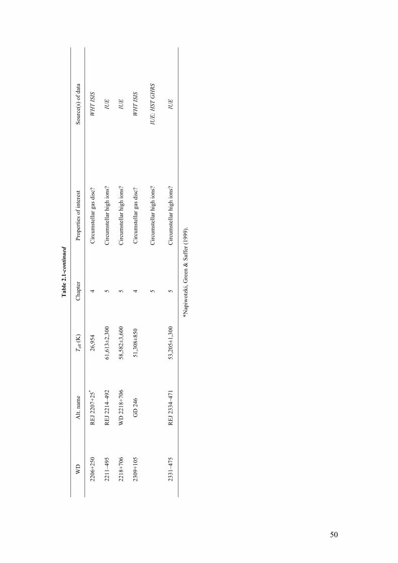
50
Sour
ce(s
) of d
ata
WH
T IS
IS
IUE
IUE
WH
T IS
IS
IUE;
HST
GH
RS
IUE
Prop
ertie
s of i
nter
est
Circ
umst
ella
r gas
dis
c?
Circ
umst
ella
r hig
h io
ns?
Circ
umst
ella
r hig
h io
ns?
Circ
umst
ella
r gas
dis
c?
Circ
umst
ella
r hig
h io
ns?
Circ
umst
ella
r hig
h io
ns?
Cha
pter
4 5 5 4 5 5
T eff (K
)
26,9
54
61,6
13±2
,300
58,5
82±3
,600
51,3
08±8
50
53,2
05±1
,300
Alt.
nam
e
REJ
220
7+25
*
REJ
221
4–49
2
WD
221
8+70
6
GD
246
REJ
233
4–47
1
Tab
le 2
.1-c
ontin
ued
W
D
2206
+250
2211
–495
2218
+706
2309
+105
2331
–475
*Nap
iwot
zki,
Gre
en &
Saf
fer (
1999
).

51
Chapter 3
Stratified metals in hot white dwarf
atmospheres?
3.1. Introduction.
Inconsistent results have been obtained from investigations into the
stratification of metals in the DAs WD 1029+537, WD 1614–084 and WD 0050–332.
Some evidence exists for similar metal stratification in WD 0948+534 (Section 1.7.2).
This is of particular interest, as the extraordinary metal abundances of these stars have
been linked to the presence of circumstellar material by some authors (e.g. Section
1.7.3). Therefore, a clear understanding of what the photospheric abundances and
distributions of such metals are is needed, to see if novel metal distributions exist in
the stars in question.
The observations and methods used to examine the metal distributions in the
stars are detailed in Section 3.2. The results for the stars in which nitrogen was
studied are presented in sections 3.3–3.5; an examination of the metals in WD
0948+534 follows in Section 3.6. The results are discussed in 3.7 with a summary in
Section 3.8.

52
3.2. Observations and method.
The observations used here are listed in Table 3.1. Models of WD 1029+537,
WD 1611–084 and WD 0050–332 were computed using TLUSTY, with the Teff, log g
and carbon, oxygen and silicon abundances in Table 3.1. Model ions for C III, C IV,
N III, N IV, N V, O IV, O V, O VI, Si III, and Si IV were explicitly included (i.e. full
model ions with all transitions and oscillator strengths, etc, were used), while C V, N
VI, O VI and Si V were treated as one level ions. One level ions are used for the
highest ion of each element to provide a simpler method of ionisation balance
calculation without having to consider detailed partition functions for the highest ions
(which for massive ions can become rather complex and cumbersome); in stars with
high Teff and massive, non-hydrogenic elements the complex transitions that occur in
the high ions of such heavy elements are not included in the models, in an analogous
fashion to the use of superlevels. In a similar situation to the use of superlevels, these
approximations may lead to some inaccuracies in atmosphere calculations where
highly ionised, massive ions are present. Model grids were constructed to cover a
range of nitrogen abundances spanning those measure by both Barstow et al. (2003b)
and Chayer, Vennes & Dupuis (2005), rather than focusing on just the high
abundance regime as in Barstow et al. (2003b), to allow a full examination of the
evolution of the N V doublet and EUV continuum with nitrogen abundance.
FUV spectra were synthesised using SYNSPEC, from 1235 – 1245 Å to cover
the N V doublet. XSPEC was used to fit the model spectra to the data. When a best
fitting nitrogen abundance was found, a set of stratified models were constructed,
with the best fitting nitrogen abundance at the top of the atmosphere and an

53
abundance of zero below. In each model, the depth of this layer was extended,
allowing a model grid to be constructed to investigate whether a stratified metal
configuration better represented the data than a homogeneous one (it must be
emphasised that the stratification of the metals here was not self-consistently
formulated like the depth dependent models of Dreizler 1999, Dreizler & Wolff 1999,
Schuh, Dreizler & Wolff 2002 and Schuh, Barstow & Dreizler 2005, but were
‘exploratory’ stratified models such as those of Hubeny & Holberg 1998 and Holberg
et al. 1999a). The EUV analysis was conducted in the EUVE SW range (80 – 180 Å),
since the EUV continuum absorption is most severe in this region. Again, XSPEC
was used to fit the data. Interstellar absorption was charaterised using the column
densities quoted in Table 3.1.
The FUV absorption features (Table 3.2) in the spectrum of WD 0948+534
were fit using the model grids used by Barstow et al. (2003b). Once initial abundance
estimates were made, models with stratified metals were produced for C, N, O and Si
in the same way as the nitrogen model grids constructed for the other three stars. The
iron and nickel abundances measured by Barstow et al. (2003b) were included in all
models of this object. Fe IV, Fe V, Fe VI, Ni IV, Ni V and Ni VI were included
explicitly, with Fe VII and Ni VII treated as one level ions. Spectra around the
wavelengths stated in Table 3.2 were again synthesised using SYNSPEC.

54
Table 3.1. The observation information, stellar and ISM parameters for the white
dwarfs studied here (unless stated otherwise, all data are from Barstow et al. 2003b).
The absence of data signifies where a measurement was unobtainable, either due to
lack of spectral coverage or an inability to model the absorption features.
WD 0050–332 0948+534 1029+537 1611–084
Mode E140H E140M E140M G160M STIS
data %% (Å) 1159, 1357 1150, 1729 1150, 1729 1386, 1423
Mode SW SW EUVE
data %% (Å) 80, 180
80, 180
Teff (K) 35,660 110,000 44,350 38,840
log g 7.93 7.58 7.81 7.92
C III/H 0.00 3.00x10⁻⁷
C IV/H 5.00x10⁻⁸ 1.60x10⁻⁷ 7.00x10⁻⁷
N V/H 6.30x10⁻⁴ 5.00x10⁻⁵ 2.50x10⁻⁴
N V/Ha 6.31x10⁻⁶ 1.26x10⁻⁶ 6.31x10⁻⁷
O V/H 0.00 1.20x10⁻⁷
Si IV/H 4.80x10⁻⁹ 9.50x10⁻⁷ 9.50x10⁻⁹
Fe V/H 0.00 1.90x10⁻⁶ 0.00 0.00
Ni V/H 0.00 1.20x10⁻⁷ 0.00 0.00
log(NH I) (cm–2) 18.46b 18.62c
log(NHe I) (cm–2) 17.37b 17.75c
log(NHe II) (cm–2) 17.17b 17.28c
aChayer et al. (2005), bBarstow et al. (1997), cHolberg et al. (1999b).

55
Table 3.2. The laboratory wavelengths of the FUV absorption features examined
here5.
Ion Lab. Wavelength (Å)
C IV 1548.187, 1550.772
N V 1238.821, 1242.804
O V 1371.296
Si IV 1393.755, 1402.770
3.3. WD 1029+537.
The FUV N V doublet yields a best fitting nitrogen abundance of
3.39
!
"1.31+1.29x10⁻⁷ with the homogeneous grid (Figure 3.1), with a
!"2 of 0.58. A
secondary minimum was also found at 5.00
!0.48+2.55x10⁻⁵, with a
!"2 of 0.77. Forcing the
nitrogen to a stratified configuration does not produce a significant improvement over
the lower abundance, homogeneous fit.
An analysis was also performed of the EUVE data of this object. To account
for the interstellar absorption observed in the EUVE dataset, the hydrogen and helium
columns from Table 3.1 were used in the modelling process. The EUV spectrum
generated using a homogeneous N/H of 3.39x10⁻⁷ is shown in Figure 3.2; the data are
represented well when compared to the Holberg et al. (1999a) homogeneous model
(Figure 1.6, lower curve).
5 wavelengths taken from the Kurucz database (http://www.pmp.uni-hannover.de/cgi-bin/ssi/test/kurucz/sekur.html).
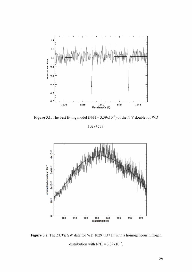
56
Figure 3.1. The best fitting model (N/H = 3.39x10⁻⁷) of the N V doublet of WD
1029+537.
Figure 3.2. The EUVE SW data for WD 1029+537 fit with a homogeneous nitrogen
distribution with N/H = 3.39x10⁻⁷.

57
3.4. WD 1611–084.
Like WD 1029+537, two best fitting abundances are seen in the N V doublet
fits of WD 1611–084 (Figure 3.3). The higher abundance model
(N/H = 3.41
!1.50+1.81x10⁻⁴) produces the global
!"2 minimum (
!"2 = 1.13; Figure 3.3, upper
panel), while the secondary best fit was found at N/H = 1.76
!1.26+1.65x10⁻⁶ (
!
"#2 = 1.21;
Figure 3.3, lower panel). The lower abundance model over predicts the depths of
observed line profiles, while the N V absorption features of the higher abundance
model do not quite extend into the observed line profiles. No EUVE data exists for
this object.
Figure 3.3. The lower nitrogen abundance model (N/H = 1.76x10⁻⁶,
!"2 = 1.21) of
WD 1611–084 is shown in the upper panel. The lower panel shows the high
abundance model (N/H = 3.41x10⁻⁴;
!"2 = 1.13).

58
3.5. WD 0050–332.
In keeping with the results of WD 1029+537, WD 0050–332 is better fit with
a lower abundance, homogeneous model. The overall best fit is found at
N/H = 6.05
!0.62+0.64x10⁻⁷ (
!"2 = 2.15; the best fitting model of the N V doublet is shown in
Figure 3.4), with a secondary best fit at 5.70
!0.62+0.41x10⁻⁵ (
!"2 = 2.41). Again, the higher
abundance, stratified model does not offer any improvement over the lower
abundance, homogeneous model. The EUVE data are again well fit by the lower
abundance, homogeneous model.
Figure 3.4. The best fitting model (N/H = 6.05x10⁻⁷,
!"2 = 2.15) of the N V doublet
of WD 0050–332.

59
3.6. WD 0948+534.
The line profiles of the best-fit models do not reproduce the data well (e.g.
Figure 3.5). The best fitting abundances are given in Table 3.3; above these
abundances the model line profiles do not reproduce the narrow widths of the
observed lines, and the NLTE core emission developing in the short wavelength
component of the N V doublet in Figure 3.5 becomes more severe (due to the
emission caused by the temperature inversion seen in NLTE atmospheres; Lanz &
Hubeny, 1995). Stratification of the metals does not improve the model fits.
Table 3.3. The estimated metal abundances for WD 0948+534. Given the poor match
to the data, errors were not computed for these models.
C IV N V O V* Si IV
4.85x10⁻⁶ 1.6x10⁻⁶ 3.5x10⁻⁵ 3.15x10⁻⁵
*this abundance is the grid upper limit
3.7. Discussion.
The modelling of nitrogen in the photospheres of WD 1029+537, WD 1611–
084 and WD 0050–332 displays a degeneracy, where more than one minimum is
present in the distribution of the fit (the abundances adopted in this study are
given in Table 3.4; the reasons for those abundance choices are detailed in the
following discussion). The absorption line profiles of WD 0948+534 are not well
modelled here.
!"2

60
Figure 3.5. The N V doublet of WD 0948+534, fit with a model with N/H = 1.6x10⁻⁶.
The
!"2 distribution of WD 1029+537 is shown in Figure 3.6. The upper panel
shows the full
!"2 distribution, with a clear, global minimum at N/H = 3.39x10⁻⁷
(
!"2 = 0.58). A secondary minimum is seen at N/H = 5.00x10⁻⁵ (
!"2 = 0.77). The
minima are shown in more detail in the lower panel of Figure 3.6. The global and
secondary minima are clearly separated, with the secondary minimum well above the
3& confidence limit (dotted line) of the global minimum (dashed line). The EUVE SW
data are also well fit with the lower abundance model. A similar situation is seen at
WD 0050–332, with a
!"2 global minimum at N/H = 6.05x10⁻⁷.

61
Table 3.4. The best fitting nitrogen abundances for WD 1029+537, WD 1611–084
and WD 0050–332 adopted in this study.
Star N/H
WD 1029+537 3.39
!
"1.31+1.29x10⁻⁷
WD 1611–084 1.76
!
"1.26+1.65x10⁻⁶
WD 0050–332 6.05
!
"0.62+0.64 x10⁻⁷
Two minima are also seen in the
!"2 distribution of WD 1611–084 (Figure
3.7), although they were less easy to disentangle. The lower panel of Figure 3.7 shows
that the difference between the two
!"2 minima is not greater than 3& confidence limit
of the global minimum. Indeed, unlike WD 1029+537 and WD 0050–332, the global
!"2 minimum for WD 1611–084 is found in the higher abundance regime (N/H =
3.41
!1.50+1.81x10⁻⁴). Poorly defined minima can also be seen at N/H = 10–5 and 7x10⁻³.
Since WD 1029+537 and WD 0050–332 are well explained using a low abundance,
homogeneous nitrogen model, the lower abundance model was also adopted for WD
1611–084. Data with a better signal to noise ratio may allow this degeneracy to be
broken with more certainty.
An examination of the model NLTE population responsible for the N V
doublet (2S) and the N VI level shows that as the nitrogen abundance in WD
1029+537, WD 1611–084 and WD 0050–332 is increased, the value of
log(N V(2S)/ N VI) begins to decrease above N/H = ~10–6 (Figure 3.8). This ‘over-
ionisation’ of nitrogen may provide a mechanism for the apparent degeneracy to arise;

62
as the nitrogen abundance increases the relative amount of N V (2S) to N VI
decreases. The trend seen in the log(N V(2S)/ N VI) of WD 1029+537 and WD 0050–
332 is also seen in WD 1611–084, providing further support for a lower N/H in WD
1611–084.
Figure 3.6. The
!"2 distribution of WD 1029+537 as N/H is increased. The global
minimum is represented with a dashed line, and its 3& confidence limit is denoted
with a dotted line.

63
Figure 3.7. The
!"2 distribution of WD 1611–084. The line representations are the
same as in the previous figure.
Papers (e.g. Holberg et al. 1999a) that report high abundance, stratified
nitrogen in the spectra of the stars cite radiatively driven mass loss acting on the
photospheric nitrogen, enriching the upper atmosphere. Studies of mass loss in DA
white dwarfs suggest that the radiative acceleration in white dwarfs in the Teff range
studied here cannot overcome the log g of the stars (Unglaub 2007, 2008). Given that
no circumstellar nitrogen is seen at WD 0050–332, WD 1029+537 and WD 1611–084
(Bannister et al. 2003; Chapter 6 of this thesis), there is no mechanism for the

64
enrichment of the upper atmospheres of these stars, further strengthening the
argument that the stars have homogeneous nitrogen distributions. Another reason for
the degeneracy seen here may be the use of the one level ions for the highest
ionisation stages (though were to be an issues one may expect to see this effect in the
absorption features in hotter stars). The development of more complex model ions is a
subject of ongoing research; as this work progresses tests of more detailed model ions
on stars such as these may provide the observed absorption line profiles.
Figure 3.8. The change in the log of the ratio of the NLTE population responsible for
the N V doublet (2S) to the N VI level population, with nitrogen abundance. Note that
not all of the model grids span the same abundance range; models were only
computed over the range required to explain the observations.
A comparison of the nitrogen abundances found here to those measured by
Barstow et al. (2003b) and Chayer, Vennes & Dupuis (2005) is shown in Figure 3.9.

65
The new results are in keeping with those found by Barstow et al. (2003b), for the
stars with higher Teff. The trend of increasing N/H with decreasing Teff seen by
Barstow et al. (2003b) is not seen. The abundances measured by Chayer, Vennes &
Dupuis (2005) are closer to those found here (although they are offset, probably due
to systematic differences in the fitting procedure used by Chayer, Vennes & Dupuis,
2005). Figure 3.10 shows a comparison of the N/H values derived here to the
radiative levitation predictions of Chayer et al. (1995); the abundances found here are
closer to those predicted than those of Barstow et al. (2003b), where the stars had a
stratified, high nitrogen abundance, with a trend of decreasing abundance with Teff.
Figure 3.9. A comparison of the nitrogen abundances found here (triangles) to those
found by Barstow et al. (2003b; filled circles) and Chayer et al. (2005; open circles).
The dotted lines connect multiple measurements of individual stars for ease of
comparison.

66
Figure 3.10. A comparison of the N/H values found here, by Barstow et al. (2003b)
and Chayer et al. (2005), to the radiative levitation predictions of Chayer et al. (1995).
The plot symbols are the same as in the previous figure.
Since homogeneous models with unremarkable abundances explained the
observed N V doublets of WD 1029+537, WD 1611–084 and WD 0050–332 well, it
is perhaps unsurprising that stratified models with high metal abundances failed to
reproduce the line profiles of metallic high ions in WD 0948+534. Indeed, the
!"2
distributions for the C IV, N V, O V and Si IV abundances of WD 0948+534 had
single minima at the abundances detailed in Table 3.3. One possible explanation is
that a physical effect that becomes significant at high Teff may be missing from the
models. Given the much higher Teff of WD 0948+534 when compared to the other
stars, this omission may cause the model-observation disagreement. The lack of

67
detailed model ions for high ionisation stages may also cause a problem (particularly
for Fe peak elements), as the lack of detailed ionisation and excitation equilibrium
calculations may have a significant effect on the atmospheric structure. In addition to
this, the lack of inclusion of small amounts of other heavier elements, such as Ar VII,
Ge IV and possibly Sn IV that have recently been found in this DA (Werner, Rauch &
Kruk, 2007) and others such as WD 0501+527 (Vennes, Chayer & Dupuis 2005),
may also have an effect on the atmosphere model calculations, should the combined
effect of all these ions on the structure of the atmosphere be significant. As more
exotic metals are discovered in hot DA spectra and more detailed model ions become
available they should be included in model calculations of this star to test this
possibility. Another possibility is that some other material is present along the line of
sight to the white dwarf, with a velocity unresolved from that of the photosphere (a
hint of a secondary component can be seen in the C IV doublet near 1548.3 Å and
1550.9 Å; Figure 1.10). This is explored in Chapter 5.
3.8. Summary.
• Previous studies came to conflicting conclusions as to the abundance and
distribution of photospheric nitrogen in WD 1029+537, WD 1611–084 and WD
0050–332.
• These stars were re-examined, and a degeneracy in nitrogen abundance is seen,
with more than one minimum in the nitrogen abundance
!"2 distribution. The N V
doublets of WD 1029+537 and WD 0050–332 are better fit with lower

68
abundance, homogeneous nitrogen. The degeneracy is difficult to break in the
case of WD 1611–084. However, the lower abundance model is assumed.
• An examination of the model NLTE populations shows that as N/H increases, the
values of log(N V(2S)/N VI) decrease in all three stars. This could explain the
observed degeneracy.
• Mass loss is predicted to not occur at these stars, and circumstellar material is not
present from which the upper atmospheres of the stars can be enriched,
strengthening the argument for homogeneous, lower abundance nitrogen
distributions.
• The abundances measured here follow the predictions of radiative levitation
theory better than those measured by Barstow et al. (2003b).
• The high ion absorption features of WD 0948+534 cannot be satisfactorily
matched with the model sets used here. This could be to an unaccounted for high
Teff effect, or unresolved, non-photospheric C IV along the sight line to the star.
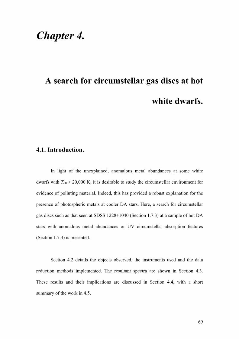
69
Chapter 4.
A search for circumstellar gas discs at hot
white dwarfs.
4.1. Introduction.
In light of the unexplained, anomalous metal abundances at some white
dwarfs with Teff > 20,000 K, it is desirable to study the circumstellar environment for
evidence of polluting material. Indeed, this has provided a robust explanation for the
presence of photospheric metals at cooler DA stars. Here, a search for circumstellar
gas discs such as that seen at SDSS 1228+1040 (Section 1.7.3) at a sample of hot DA
stars with anomalous metal abundances or UV circumstellar absorption features
(Section 1.7.3) is presented.
Section 4.2 details the objects observed, the instruments used and the data
reduction methods implemented. The resultant spectra are shown in Section 4.3.
These results and their implications are discussed in Section 4.4, with a short
summary of the work in 4.5.

70
4.2. Observations and data reduction.
The white dwarfs observed (selected due to their unusual metal abundances)
are detailed in Table 4.1. The observations were made by M. Burleigh on the nights of
the 6th and 7th of August 2007, at the William Herschel Telescope (WHT) on La
Palma. Both the red and blue arms of the ISIS spectrometer were used, with the
R1200 grating. The data were reduced in IRAF, using standard subroutines for the
reduction of long slit spectroscopy.
Table 4.1. The white dwarfs observed in this study. The right ascension (RA) and
declination (DEC) (J2000) of each star are from the McCook & Sion online catalog6.
The Teff values are from the references detailed.
WD number Alt. name Teff (K) RA DEC
WD 0004+330 GD 2 47,219a 00 07 32.3 +33 17 27
WD 0209+085 HS 0209+083 36,000b 02 12 04.8 +08 46 51
WD 1614–084 REJ 1614–085 38,840±480c 16 14 19.0 –08 33 27
WD 1942+499 REJ 1943+50 34,056a 19 43 42 +50 04 41
WD 2032+248 Wolf 1346 19,150±30c 20 34 22.3 +25 03 58
WD 2111+498 GD 394 39,290±360c 21 12 43.8 +50 06 17
WD 2205+250 REJ 2207+25 26,964d 22 07 44.8 +25 20 22
WD 2309+105 GD 246 51,308±850c 23 12 21.5 +10 47 04
aMullally et al. (2007) and references therein, bJordan et al. (1993), cBarstow et al.
(2003b), dNapiwotzki, Green & Saffer (1999).
6 http://astronomy.villanova.edu/WDcatalog/index.html

71
4.3. Results.
The spectral region containing the Ca II triplet (8350–8800 Å) is shown in
Figure 4.1, for all stars. Similarly, the spectral region containing the Mg II absorption
line (4470–4490 Å) is shown in Figure 4.2. No emission from Si III or Fe II is seen,
although absorption from Fe II (5020 Å) and Si III (4552 Å, 4568 Å) is detected in
the spectra of WD 0209+085 and WD 2111+498, respectively (Figure 4.3).
4.4. Discussion.
No Ca II emission is seen in the spectra of the stars in this sample (Figure 4.1).
However, the spectrum of WD 1942+499 is contaminated by a cosmic ray around
4482 Å (Figure 4.2), which might prevent the detection of Mg II absorption. Although
Si II and Fe II absorption is seen at WD 2111+498 and WD 0209+085 (Figure 4.3),
respectively, no emission lines are detected from these ions. Mullally et al. (2007)
found no evidence for infrared excesses in the spectra of these stars. However, such
excesses are present at no more than 20% of the cooler DAZ stars with metal
abundances indicative of ongoing accretion (Farihi, Jura & Zuckerman, 2009),
suggesting that the small sample size here may be responsible for a lack of such
detections.
While no firm detections of circumstellar discs have been achieved here,
many questions remain as to origin and abundance of the metals in these objects. WD
2111+498 (which has no binary companion from which metals can be accreted; Saffer
et al. 1998) has an anomalously high silicon abundance (~100 times that of other DAs
with a similar Teff; Holberg et al. 1997), and its iron abundance is higher than that of

72
WD 0232+035 and WD 0501+527 (Vennes et al. 2006). Given that these DAs have
Teff values both significantly above that of WD 2111+498 and above 50,000 K (at
which point radiative levitation becomes dominant), they are expected to have much
higher metal abundances than WD 2111+498 (Chayer et al. 1995). WD 2111+498
cannot be modelled using the self-consistent, stratified models calculated by Schuh,
Dreizler & Wolff (2002); this has been attributed to the accretion of circumstellar
material disturbing the diffusion/levitation balance. This body of evidence strongly
suggests the photosphere of WD 2111+498 is being enriched by the accretion of
circumstellar metals. A periodic EUV variability (p = 1.150±0.003 days; Dupuis et al.
2000), suggests this accretion is inhomogeneous (possibly polar, although no
significant magnetic field has been detected). However, since both this study and
previous studies (e.g. Bannister et al. 2003) have not detected circumstellar metals,
the source of accreted material at this star remains, thus far, a mystery. Similarly, the
photospheric aluminium and silicon abundances of WD 2023+246 are in excess of
those predicted by radiative levitation theory (Chayer & Dupuis, 2010; Dupuis,
Chayer & Hénault-Brunet, 2010),
However, although no gas disc is detected here, non-photospheric absorption
features inconsistent with the ISM along the sight line to WD 1611–084 are present
(Holberg, Barstow & Green, 1997; Bannister et al. 2003). These features have, in
keeping with WD 1620–391 (CD –38 10980; Holberg, Bruhweiler & Andersen 1995),
been attributed to circumstellar material.

73
Figure 4.1. The spectral region containing the Ca II triplet. Each data set is
normalised and offset for clarity.

74
Figure 4.2. The spectral region containing the Mg II 4482 Å absorption line. The
gaps in the spectrum of WD 1942+499 are due to the removal of cosmic ray
contamination.

75
Figure 4.3. The upper panel shows the Fe II absorption (5020 Å) in the spectrum of
WD 0209+085, while the bottom panel shows the Si III absorption features (4552 Å,
4568 Å) in the spectrum of WD 2111+498.
.

76
Further work is needed to understand the circumstellar environment of hot
white dwarf atmospheres. An examination of the ‘circumstellar’ features seen by
Bannister et al. (2003) is presented in the next Chapter, in an attempt to better
understand the origin of these features and how they may relate to the observed white
dwarf metal abundances.
4.5. Summary.
• Gaseous components to circumstellar dust discs have been detected at some
white dwarfs. Accretion from circumstellar discs is used to explain the metal
pollution of cooler DA stars (Teff < 20,000 K).
• A search for gas discs at hotter stars with metal abundances in excess of those
predicted by radiative levitation is undertaken here, where one would expect
any circumstellar discs present to have sublimated, in an attempt to identify a
source of accretion.
• No circumstellar gas emission is detected.
• The stars still have metal abundances that cannot be explained by radiative
levitation alone, and in some cases (such as WD 2111+498) the metal
abundances are far higher than those found for other, hotter white dwarfs,
Since circumstellar disc detection (via infrared excess emission) has only been
achieved for approximately 20% of the cooler stars where accretion of metal

77
rich material is required to explain the presence of photospheric metals, it may
be the case that the lack of circumstellar gas detection here is related to the
small sample size.

78
Chapter 5.
The origin of ‘circumstellar’ features in hot
DA white dwarf spectra.
5.1. Introduction.
As discussed at length in Section 1.7.3, circumstellar absorption features have
been observed in the spectra of hot DA white dwarfs. This Chapter re-examines the
sample of Bannister et al. (2003), using a more advanced absorption line profile
modelling technique. The results of this examination are compared to different
physical scenarios in which circumstellar absorption may occur, including material in
a circumstellar disc, the ionisation of ISM in the locality of the star, stellar mass loss
and ancient PNe.
Section 5.2 details the sample and the method used to analyse it, while the
results are presented in 5.3. The results are discussed in 5.4; a sub-section details
each physical scenario (circumstellar discs, 5.4.1; ISM ionisation, 5.4.2; mass loss,
5.4.3; ancient PNe 5.4.4) in which such absorption may arise. A summary of the
results and conclusions is presented in 5.5.

79
5.2. Observations and modelling circumstellar absorption
components.
The white dwarfs studied were those included in the Bannister et al. (2003)
sample; stellar parameters and observation details can be found in Table 5.1. The high
ionisation stage absorption lines examined were the same as those studied in Chapter
3, and were detailed in Table 3.2. Where circumstellar absorption was observed, the
O VI doublet (1031.912 Å, 1037.613 Å) in the FUSE spectrum (R = 20,000) of each
object was examined, where data were present and the features exist.
The method used here to measure the absorption line components has been
described extensively in studies of the ISM (e.g. Welsh & Lallement 2005, 2010;
Welsh et al. 2010a,b). The absorption line profiles were fit with Gaussian absorption
components. Non-photospheric absorption components were added when the fit was
improved in a statistically significant way, i.e. if the probability of similar
improvement in the fit upon inclusion of the additional component (
!" 2 = 11.1)
being random was less than 1 % (Vallerga et al. 1993). The software used to make
the measurements was written by, and is proprietary to, B. Welsh and R. Lallement.
B. Welsh carried out the fitting, under guidance (the target list, lines of interest and
objects at which previous circumstellar detections were made was provided).

80
Res
olvi
ng P
ower
100,
000;
20,
000
40,0
00
20,0
00
40,0
00
40,0
00
20,0
00
40,0
00
40,0
00
40,0
00
22,0
00
100,
000
20,0
00
20,0
00
20,0
00
22,0
00
40,0
00
20,0
00
20,0
00; 2
2,00
0
40,0
00
20,0
00
40,0
00
40,0
00; 2
0,00
0
20,0
00
Dat
a so
urce
[Mod
e]
STIS
[E14
0H];
IUE
[SW
P]
STIS
[E14
0M]
IUE
[SW
P]
STIS
[E14
0M]
STIS
[E14
0M]
IUE
[SW
P]
STIS
[E14
0M]
STIS
[E14
0M]
STIS
[E14
0M]
GH
RS [G
160M
]
STIS
[E14
0H]
IUE
[SW
P]
IUE
[SW
P]
IUE
[SW
P]
GH
RS [G
160M
]
STIS
[E14
0M]
IUE
[SW
P]
IUE
[SW
P]; G
HRS
[G16
0M]
STIS
[E14
0M]
IUE
[SW
P]
STIS
[E14
0M]
STIS
[E14
0M];
IUE
[SW
P]
IUE
[SW
P]
D (p
c)b
53
78
108
50
295
97
217
193.
8
127
411
147
73
71
25
86
243
14
57
129
69
436
72
104
L/Lb
0.24
5.86
1.85
3.16
4.61
11.6
9
10.1
9
1.03
0.64
2.75
0.56
1.49
0.03
0.43
12.5
9
0.03
0.45
1.06
9.38
9.64
2.23
2.88
log
ga
7.93
±0.0
3
7.50
±0.0
6
7.93
±0.0
8
7.53
±0.0
9
7.70
±0.0
9
7.14
±0.1
1
7.47
±0.0
5
7.58
±0.0
6
7.81
±0.0
8
7.90
±0.1
0
7.48
±0.0
8
7.77
±0.0
5
7.85
±0.0
7
8.05
±0.0
1
7.92
±0.0
7
7.77
±0.1
0
7.91
±0.0
1
7.89
±0.0
5
7.86
±0.1
0
7.29
±0.1
1
7.05
±0.1
2
7.91
±0.0
7
7.67
±0.1
0
T eff (K
)a
35,6
60±1
35
60,4
87±1
,100
50,9
60±1
,070
52,5
00±9
00
59,5
08±2
,200
58,2
00±1
,800
69,7
11±5
30
110,
000±
2,50
0
44,3
50±7
15
39,7
70±6
15
54,5
74±9
00
39,2
90±3
40
50,3
70±8
70
22,0
90±8
5
38,8
40±4
80
66,7
60±1
,230
19,1
50±3
0
39,2
90±3
60
45,5
00±1
,085
61,6
13±2
,300
58,5
82±3
,600
51,3
08±8
50
53,2
05±1
,300
Alt.
nam
e
GD
659
Feig
e 24
REJ
045
7–28
1
G19
1-B
2B
REJ
055
8–37
3
REJ
062
3–37
1
Ton
021
PG 0
948+
534
REJ
103
2+53
2
PG 1
057+
719
PG 1
123+
189
GD
153
HZ
43
EG 1
02
REJ
161
4–08
5
REJ
173
8+66
5
Wol
f 134
6
GD
394
REJ
215
6–54
6
REJ
221
4–49
2
WD
221
8+70
6
GD
246
REJ
233
4–47
1
Tab
le 5
.1. T
he st
ella
r par
amet
ers a
nd o
bser
vatio
n in
form
atio
n fo
r the
DA
s stu
died
her
e.
WD
0050
–335
0232
+035
0455
–282
0501
+527
0556
–375
0621
–376
0939
+262
0948
+534
1029
+537
1057
+719
1123
+189
1254
+223
1314
+293
1337
+705
1611
–084
1738
+669
2023
+246
2111
+498
2152
–548
2211
–495
2218
+706
2309
+105
2331
–475
a from
Bar
stow
et a
l. (2
003b
) ; b fr
om B
anni
ster
et a
l. (2
003)
and
refe
renc
es th
erei
n.

81
The details of the absorption line modelling process are outlined in several
papers (e.g. Vallerga et al. 1993; Sfeir et al. 1999), and a summary is presented here.
The local continuum was characterised with a multi-order polynomial fit (absorption
features were neglected), with the root mean square of the fit adopted temporarily as
the error of each data point. The
!"2 of the continuum model was calculated, and the
errors on the data points previously assigned were adjusted by a constant factor until
the
!"2 was equal to 1.0. Errors on the fit to absorption feature were derived in a
similar way (where the model Gaussian absorption components were included),
allowing both the line profiles and continuum placement to be taken into account in
the error calculation. The equivalent width of the absorbing component was
calculated by integrating the absorbed flux in the absorption feature, propagating the
error on the model data points.
The heliocentric velocities of the absorption components were allowed to
vary simultaneously (note that in the case of the data used here, no heliocentric
correction was applied since data from IUE, HST and FUSE are expressed in the
heliocentric frame) through a "2 minimisation technique, as was the broadening of the
absorption line component (b). The column densities (N) of the circumstellar and
interstellar material were derived as part of the line fitting routine. The measured
equivalent widths and the oscillator strengths of the absorption lines were used to
generate theoretical line profiles, which were fit to the absorption features to provide
column densities. Reliable errors were produced for unsaturated line profiles. Since
the oscillator strengths were used to model the absorption lines, the technique used by
Bannister et al. (2003) of coadding absorption features in velocity space to improve

82
the signal to noise and reveal hidden circumstellar components cannot be utilised
here.
Bannister et al. (2003) used the curve of growth method to measure
circumstellar column densities. In this method, the change in equivalent width with
column density is calculated for the absorbing material, for a series of b values. The
observed equivalent widths are then plotted on the curve corresponding to the
measured b value and the column density is read off. This does method does not
explicitly model the observed line profiles using the line transition data, making the
work here a significant improvement over Bannister et al.’s (2003) previous study.
The velocities of the photospheric components of each high ion absorption
line were measured (where present), and the mean of these measurements was
calculated to give the averaged photospheric velocity (vphot) of the star. Likewise,
when circumstellar components were seen in the absorption line profiles, the mean of
the measured velocities was calculated to produce a characteristic circumstellar
velocity (vCS) for the absorbing material. To characterise the ISM velocity, the
velocities of unsaturated absorption lines (such as Si II; 1260.422 Å, 1304.370 Å and
S II; 1259.52 Å) were measured since more accurate line properties could be derived.
When additional measurements were required (e.g. where Si II or S II were not
present), other low ion absorption lines such as O I (1302.168 Å) and Fe II
(1608.451 Å) were used. Given the variety in observed ISM composition along each
line of sight, the exact lines used varied in each case. The component with the largest
equivalent width was deemed to be the primary ISM component (with vISM,pri), the

83
next largest the secondary (with vISM,sec). Where three ISM components were present,
the component with the smallest equivalent width was denoted as the tertiary
component (with vISM,ter). Mean values of vISM,pri, vISM,sec and vISM,ter were calculated
to allow easy comparison of vCS to all interstellar components. All errors were
combined quadratically.
5.3. Results.
5.3.1. Summary of results.
Circumstellar absorption is unambiguously detected at eight white dwarfs.
The measured velocities, circumstellar velocity shifts with respect to the photosphere
(vCSshift) and gravitational redshifts (vgrav, calculated by J. Farihi using stellar masses
and radii derived from the evolutionary models of Fontaine, Brassard & Bergeron
2001) are presented in Table 5.2. Using maps of LISM morphology (Redfield &
Linsky, 2008), the LISM clouds along each white dwarf sight line are identified and
their projected velocity (vLISM) is included7 in the sixth column of Table 5.2. This
allows the detected circumstellar and ISM component velocities to be compared to
vLISM, to examine any possible links the detected absorption may have to LISM
clouds. Table 5.3 details which ions display circumstellar components, and gives their
column densities. Detailed notes on the results for each object follow Tables 5.2 and
5.3. The objects grouped into those with circumstellar detections (Section 5.3.2), and
those without (Section 5.3.3). 7the cloud identification and velocity projections were performed using the online tool available at http://lism.wesleyan.edu/LISMdynamics.html

84
v gra
v
28.2
1
15.7
28.9
6
16.0
7
21.0
7
9.36
15.4
0
19.6
7
24.0
0
27.1
8
14.9
8
22.3
6
25.7
7
32.8
4
27.9
5
23.6
5
26.4
1
26.7
7
25.9
11.4
3
8.04
28.1
7
19.8
8
v LIS
M (c
loud
nam
e)*
4.56
±1.3
6 (L
IC)
18.1
±1.1
3 (L
IC)
12.5
6±1.
03 (B
lue)
19.1
±1.1
(LIC
), 9.
35±1
.32
(Hya
des)
11.3
6±0.
95 (B
lue)
11.0
9±0.
93 (B
lue)
10.8
1±1.
29 (L
IC)
10.0
7±1.
31 (L
IC)
7.72
±1.3
3 (L
IC)
6.64
±1.3
5 (L
IC)
3.03
±0.7
9 (L
eo)
–5.5
2±0.
74 (N
GP)
–6.1
5±0.
74 (N
GP)
1.59
±1.3
8 (L
IC)
–29.
26±1
.12
(G)
–2.9
1±1.
37 (L
IC)
–2.3
5±1.
38 (L
IC)
–9.7
3±1.
31 (L
IC)
–8.8
±1.3
2 (L
IC),
9.93
±0.6
(Dor
)
4.47
±1.3
7 (L
IC)
–8.2
±0.7
0
–3.4
1±1.
37 (L
IC)
v ISM
(pri,
sec,
ter)
6.7±
0.3
2.85
±0.3
4, 1
7±1.
3
12.1
±1.5
8.15
±0.1
8, 1
9.3±
0.03
7.8±
1
15.8
±0.4
–2.1
±0.2
–18.
45±0
.42,
–1.
6±0.
63, 2
2.6±
0.8
0.95
±0.7
9
–0.2
±1
–4.7
5±3.
18
–15.
4±1.
8
–6.6
±0.1
–1.5
±1.8
–34.
7±1.
5
–20.
0±0.
3
–16.
3±1.
7, 1
8.3±
2.5
–7.6
±1.3
–9.2
±0.5
3
–1.1
±0.4
–15.
3±2.
64, –
1.2±
4.01
14.3
±0.7
v CSs
hift
–22.
19±0
.68a , –
120.
63±0
.40b
–60.
48±3
.90
–15.
61±0
.17
–15.
17±2
.30
–27.
12±6
.61
–25.
90±4
.11
–48.
53±4
.49
22.2
4±1.
52
v CS
7.4±
0.34
18.8
±3.4
7
8.9±
0.07
10.2
±1.0
7
9.38
±6.6
–66.
67±2
.05
–18.
36±4
.23
–17.
8±1.
05
v pho
t
34.3
4±0.
38
30.1
1±0.
52a , 1
28.2
3±0.
31b
79.2
8±1.
79
24.5
1±0.
16
25.3
7±2.
03
39.4
4±0.
25
36.5
±0.4
7
–17.
09±1
.73
37.9
8±0.
21
–40.
76±3
.56
30.1
7±1.
49
29.3
±1.6
6
–14.
94±0
.46
32.3
3±1.
37
–40.
04±1
.11
–13.
45±0
.13
38.8
8±0.
72
Tab
le 5
.2. A
ll m
easu
red
velo
citie
s, ci
rcum
stel
lar v
eloc
ity sh
ift (v
CSs
hift)
, pre
dict
ed L
ISM
vel
ociti
es a
nd g
ravi
tatio
n re
dshi
fts (v
grav
). A
ll ve
loci
ties a
re e
xpre
ssed
in k
m s-1
. W
D
0050
–335
0232
+035
0455
–282
0501
+527
0556
–375
0621
–376
0939
+262
0948
+534
1029
+537
1057
+719
1123
+189
1254
+223
1314
+293
1337
+705
1611
–084
1738
+669
2023
+246
2111
+498
2152
–548
2211
–495
2218
+706
2309
+105
2331
–475
* from
Red
field
& L
insk
y (2
008)
; a from
bin
ary
phas
e 0.
24; b fr
om b
inar
y ph
ase
0.74

85
Table 5.3. The stars with circumstellar detections, the identified species and
measured column densities.
WD Species Column density (x1012 cm–2)
0232+035 C IV 28.0±1.3
0455–282 C IV, N V, Si IV 33.2±6.6, 4.17±0.83, 3.71±0.74
0501+527 C IV 104±10
0556–375 C IV 46.8±6.2
0939+262 C IV, Si IV 8.05±0.21, 1.81±0.36
1611–084 C IV, Si IV 9.77±1.9, 3.53±0.71
1738+669 C IV, O V, O VI, Si IV 55.5±6.1, 0.235±0.029, 7.04±1.41,
3.26±0.17
2218+706 C IV, Si IV 119±17, 7.34±0.06
5.3.2. Objects with circumstellar absorption.
5.3.2.1. WD 0232+035 (Feige 24).
WD 0232+035 is part of a binary system with a dM1.5–2 companion, with a
binary period of 4.23160±0.00002 d (Vennes and Thorstensen, 1994). Data were
obtained at two phases of the binary cycle, 0.73–0.75 (29 November 1997) and
0.23 – 0.25 (4 January 1998). The mean photospheric velocity changes between data
sets (vphot(0.24) = 30.11±0.52 km s–1; vphot(0.74) = 128.23±0.31 km s–1), reflecting the
orbital motion of the white dwarf. Two sets of absorption features are seen in the C IV
doublet, one of which remains stationary at 7.4±0.34 km s–1 (vCS), and is thus the

86
circumstellar component (Figures 5.1 and 5.2). The column density for this
component is (2.8±0.13)x1013 cm–2, with a b value of 6.4±0.5 km s–1. Barstow et al.
(2010) found the single component O VI absorption line to arise in the photosphere.
Using the Si II 1304 Å and S II 1260 Å lines, a dual component ISM was
found with the primary component at 2.85±0.34 km s–1 and the secondary at
17.1±1.3 km s–1. The predicted LIC velocity is 18.1±1.13 km s–1, in keeping with the
secondary ISM component.
5.3.2.2. WD 0455–282 (REJ 0457–281).
Blue shifted features in the C IV and Si IV lines were first seen by Holberg,
Barstow & Sion (1998), and some evidence for a second absorption component in the
1238.821 Å N V line was observed by Bannister et al. (2003). The mean photospheric
velocity is detected at 79.28±1.79 km s–1, which compares well with the value of
76.91±0.83 km s–1 measured by Bannister et al. (2003). The mean velocity of the
circumstellar features is 21.76±1.27 km s–1.
The mean C IV column density is (3.32±0.66)x1013 cm–2, about one fifth of the value
(1.82x1014 cm–2) measured by Bannister et al. (2003). In addition to the C IV
column density, the mean column densities for N V and Si IV are (4.17±0.84)x1011
cm–2 and (3.71±0.74)x1012 cm–2, respectively.

87
Figure 5.1. The 1548 Å C IV line of WD 0232+025, where the binary phase is 0.24.
The circumstellar component (at 7.4 km s–1) is blended with the photospheric
components (at 30.11 km s–1). The data are plotted with a solid red line, the model
components are plotted with dotted red lines and the sum of the model components is
plotted in blue; this plotting convention is also used in Figures 5.2–5.4.
Figure 5.2. The circumstellar 1548 Å C IV line of WD 0232+025, when the binary
phase is 0.74. The photospheric component (at 128.23 km s–1) is not seen here.

88
The ISM is found at 12.1±1.5 km s–1. The line of sight to WD 0455–282
traverses the Blue cloud, which has a projected velocity of 12.56±1.03 km s–1,
implying that the ISM observed along the sight line to the star resides in the Blue
cloud. The O VI 1032 Å line displays two absorbing components, attributed to the
photosphere and blue shifted ISM by (Barstow et al. 2010).
5.3.2.3. WD 0501+527 (G191-B2B).
WD 0501+527 is among the best-studied hot white dwarfs. In keeping with
the results of Bannister et al. (2003), circumstellar C IV is observed in the STIS
[E140M] spectrum, at a velocity of 8.9±0.07 km s–1. The averaged photospheric
velocity is 24.51±0.16 km s–1. The circumstellar C IV column density is
(1.04±0.1)x1014 cm–2, a factor of four higher than the column densities found by
Bannister et al. (2003; 2.40x1013 cm–2) and Vennes & Lanz (2001; 6.31x1013 cm–2),
probably due to the fact that a curve of growth was used in those analyses, instead of
full absorption profile modelling as used here. The b value is 5.65±0.18 km s–1, near
the 5.2 km s–1 of Vennes & Lanz (2001); the higher b = 10 km s–1 reported by
Bannister et al. (2003) is inconsistent with both of these values. A single component
is detected in the O VI 1032 Å line at 19 km s–1, agreeing with other photospheric
lines in the FUSE spectrum, in keeping with both Barstow et al. (2010) and Savage &
Lehner (2006).
The interstellar components (measured using the 1259 Å S II line) are found at
8.15±0.18 km s–1 (similar to vCS) and 18.0±0.03 km s–1, agreeing with the values

89
reported for the higher resolution STIS E140H data by Sahu et al. (1999) and Redfield
& Linksy (2004). The projected LIC velocity is 19.1±1.1 km s–1, suggesting that the
LIC may account for the secondary component in the observed ISM features.
5.3.2.4. WD 0556–375 (REJ 0558–373).
Circumstellar counterparts to the photospheric C IV doublet are observed in
this 59,508 K DA. The mean photospheric and circumstellar velocities are
25.37±2.03 km s–1 and 10.2±1.07 km s–1, respectively. The average C IV column
density is (4.67±0.62) x 1013 cm–2.
The S II line is again used to characterise the ISM. Three components are seen
at 7.8±1 km s–1 (vISM, pri), 19.9±1.7 km s–1 (vISM, sec) and 36.0±2.3 km s–1 (vISM, ter).
Comparing vCSshift (–15.17±2.30 km s–1), the shift in the primary ISM component with
respect to the photosphere (–17.57±2.26 km s–1) shows an overlap in the error
margins of these quantities, implying that they may be related. The sight line to WD
0556–375 traverses the Blue cloud, which has a projected velocity of
11.36±0.95 km s–1, similar to vCS and near vISM, pri.
5.3.2.5. WD 0939+262 (Ton 021).
Circumstellar absorption is found in the C IV and Si IV doublets, giving a
mean vCS of 9.38±6.59 km s–1. When the N V doublet and the O V line are included,
vphot averages to 36.5±0.47 km s–1. The mean column density of the C IV doublet is
(8.05±0.21)x1012 cm–2 with a b value of 8.3±1.75 km s–1; with a Si IV column density

90
of (1.81±0.36)x1012 cm–2 and a b = 11.65±5.28 km s–1. These results are consistent
with the findings of Bannister et al. (2003).
Measurements of the S II ISM line characterise the ISM velocity at
–2.1±0.2 km s–1. The predicted LIC velocity is far from this value, at
10.81±1.29 km s–1.
5.3.2.6. WD 1611–084 (REJ 1614–085).
At 38,840 K, WD 1611–084 is the coolest white dwarf to show unambiguous
signs of circumstellar absorption. Photospheric C IV, N V and Si IV is observed,
yielding a mean vphot of –40.77±3.56 km s–1. The FUSE spectrum of this object
reveals a photospheric O VI 1032 Å absorption line. The column densities measured
for the circumstellar C IV and Si IV are (9.77±1.95)x1012 and (3.53±0.71)x1012 cm–2,
respectively, with b values are 4.55±2.6 and 2.3±0.46 km s–1. The velocities of the
absorption lines are inconsistent across the ions, as found by Bannister et al. (2003).
Here, the circumstellar C IV is displaced by 23.55±3.96 km s–1 with respect to the
photospheric component, while the circumstellar silicon is displaced by 30.6±0.64 km
s–1, with an averaged vCS of –66.67±2.05 km s–1.
Two components are observed in the ISM, at –34.7±1.5 (vISM,pri) and
–13±3.2 km s–1 (vISM,sec). The line of sight to WD 1611–084 traverses the G cloud,
which has a projected velocity of –29.26±1.12 km s–1, well separated from both vCS
and both ISM components.

91
5.3.2.7. WD 1738+669 (REJ 1738+665).
The mean vphot for this star is 30.49 ± 0.28 km s–1, with C IV, O V and Si IV
exhibiting clear secondary absorbing components at a mean velocity of
–18.36±4.23 km s–1. The doublet components for N V cannot be coadded to identify a
secondary absorbing component at vCS as in Bannister et al. (2003).
The column density of the C IV doublet is (5.55±0.61)x1013 cm–2 with a b
value of 6.8±0.43 km s–1; the O V and Si IV column densities are (2.35±0.29)x1011
and (3.26±0.17)x1012 cm–2, with b values of 0.3±3.8 and 6.95±1.07 km s–1. The C IV
and Si IV column densities derived by Bannister et al. (2003) using a curve of growth
were 1.70x1013 cm–2 and 1.66x1013 cm–2, both inconsistent with the values found
here. However, the values measured by Dupuis et al. (2009) were (5.01±0.48)x1013
cm–2 and (5.50±0.13)x1012 (for C IV and Si IV, respectively), and were obtained by
the apparent optical depth technique (where the observed line profiles are converted
to apparent optical depth profiles and apparent column densities per unit velocity,
providing a form of absorption line data that can be directly interpreted, e.g. Savage &
Sembach, 1991), in agreement with the column densities measured here. The ISM is
again characterised using the S II line, which has a velocity of –20±0.3 km s–1, far
from the predicted LIC velocity of –2.91±1.37 km s–1.
The FUSE spectrum shows two components in the 1032 Å O VI line, one at
–32.7±3.4 km s–1 and the other at 14.9±1.1 km s–1. The –32.7 km s–1 component is

92
adopted as circumstellar (with a column density of (7.04±1.41)x1012 cm–2 and a b
value of 12.6±5.1 km s–1) and the 14.9 km s–1 is designated the photospheric
component. This gives an O VI vCSshift of –47.6±3.6 km s–1, in agreement with the
value from the STIS measurements (–48.53±4.49 km s–1).
5.3.2.8. WD 2218+706.
Circumstellar components have previously been seen in the C IV and Si IV
doublets of this star (Bannister et al. 2003). The averaged vphot is –40.04±1.11 km s–1,
with the mean vCS at –17.8±1.05 km s–1. No O VI is seen in the FUSE spectrum of
this star. ISM components are found at –15.3±2.64 km s–1 (vISM, pri) and –1.2±4.01 km
s–1 (vISM, sec). The line of sight to WD 2218+706 traverses the LIC, which has a
projected velocity of 4.47±1.37 km s–1, nowhere near vCS or either of the ISM
components.
The circumstellar C IV column density is (1.19±0.17)x1013 cm–2 and the Si
IV column is (7.98±0.59)x1012 cm–2, with b values of 6.75±1.67 km s–1 and
11.05±2.07 km s–1. These values are somewhat different to those derived by Bannister
et al. (2003), who found C IV and Si IV column densities of 4.17x1013 cm–2 and
4.07x1013 cm–2, each with b values of 6 km s–1. However, the method used here
models the circumstellar line fully, rather than performing a curve of growth on, in
this case, two data points (Figure 6, Bannister et al. 2003).

93
5.3.3. Objects without circumstellar absorption.
5.3.3.1. WD 0050–335 (GD 659).
In this study, the mean photospheric and ISM velocities are 34.34±0.38 km s–1
and 6.7±0.3 km s–1 (using the S II 1259 Å line). A secondary component in the C IV
doublet is not seen above the noise in the data. Indeed the circumstellar component
seen by Bannister et al. (2003) was comparable to the noise in the data; the
circumstellar component was only seen when adding the doublet components in
velocity space, which cannot be achieved here. While the C IV, N V and Si IV
resonance doublets are clearly visible, the O V resonance line is not. Photospheric
O VI is detected by Barstow et al. (2010).
5.3.3.2. WD 0621–376 (REJ 0623–371).
The IUE spectrum of this 58,200 K white dwarf displays no clear
circumstellar absorption. A mean vphot of 39.44±0.25 km s–1 is found, along with a
single component ISM at 15.8±0.4 km s–1. Again, as was seen by Bannister et al.
(2003), the centroids of the components of the C IV doublet are inconsistent with one
another (v1548Å = 37.6±0.6 km s–1, v1551Å = 48.5±0.7 km s–1). Unusually (given the
high oscillator strength of the short wavelength component), the equivalent width of
the 1551 Å component (132.45 mÅ) is greater than that of the 1548 Å component
(109.75mÅ). It may be the case that some unresolved material is present along the
line of sight to this star; indeed given the poor resolving power of the IUE [SWP] data

94
(20,000), details in the line profiles may be present that instruments of a higher
resolution can resolve. A single component vISM is found at 15.8±0.4 km s–1.
5.3.3.3. WD 0948+534 (PG 0948+534).
In keeping with the findings of Bannister et al. (2003), the ISM observed
along the line of sight to this star has three absorbing components. The 1260 Å S II
line has components at –18.7±0.6 km s–1, –1.6±0.6 km s–1, and 22.6±0.8 km s–1.
When coupled with measurements of the absorbing components in the Si II 1304 Å
line, vISM,pri is found at –18.45±0.42 km s–1, vISM,sec at –1.6±0.63 km s–1 and vISM,ter
(the velocity of the tertiary ISM component) at 22.6±0.8 km s–1. In contrast, Bannister
et al. (2003) found the –1.6 km s–1 component had a larger equivalent width than the –
18.45 km s–1 component (and measured the components to be at –0.26±1.26 km s–1
and –22.8±1.2 km s–1). In the S II line, the model equivalent widths of the –18.7 km
s–1 and –0.6 km s–1 components are comparable at 32.14 mÅ and 30.99 mÅ
respectively; in the Si II line the equivalent widths of these components are 39.20 mÅ
and 25.63 mÅ, showing clearly that the –18.7 km s–1 is the primary absorbing
component.
In keeping with previous studies, one absorbing component is statistically
preferred to a two component model (i.e. the improvement in '2 obtained upon the
inclusion of a secondary component in less than 11.1; Section 5.2 of this thesis); in
the C IV doublet this is found at –16±0.3 km s–1 (Figure 5.3). All of the high ion lines
give an average vphot of –13.06 km s–1, although considerable spread is seen in the
velocities (vOV = –10.03 km s–1; vCIV = –16 km s–1). Caution must be exercised here;
95
the single model fits used here do not include stellar atmosphere models and therefore
do not reproduce physically accurate photospheric absorption line profiles. Gaussian
models are fit, showing the statistically preferred number of absorbing components.
Indeed, as detailed in Chapter 3 of this thesis, the narrow, almost saturated absorption
line profiles of the high ion absorption features are yet to be explained using stellar
models.
Although not statistically preferred, there is a hint of a second component in
the C IV doublet, putting the mean C IV photospheric component at
–17.6±0.39 km s–1 and the circumstellar C IV photospheric component at 1.65±7.22
km s–1 (Figure 5.4). Like WD 0621–375, the large inconsistencies in the centroid
positions of these absorption features might be evidence of unresolved circumstellar
absorption. Following this logic, the large spread in centroid positions in the
absorption features of this object when fit with single absorption components may
also be symptomatic of an unresolved secondary absorbing component. Applying this
to the N V, O V and Si IV (Figure 5.5) absorption features, which have photospheric
velocities of 15.4±1.35, –19.2±5.5 and 17.2±0.90 km s–1, and circumstellar velocities
of 2.0±1.39, –6.0±7.7 and 0.05±6.15 km s–1, gives a mean vphot of –17.09±1.72 km s–1
and a mean vCS of 0.2±5.40 km s–1. The large error on the mean value of vcirc is due to
a combination of the large errors on the circumstellar velocities of each ion, and the
large spread in circumstellar component velocities across the ions, possibly due to the
inability to resolve the circumstellar components here, if present.
The O VI 1032 Å line displays components at –22.9±1.2 km s–1 and
15.7±2.8 km s–1 when fit with two components. Given that the FUSE velocity

96
resolution (~15 km s–1) is poorer than that of the STIS E140M data (~7 km s–1), and
that the absolute velocity calibration of each data set is not necessarily exactly the
same, the secondary 15 km s–1 component is deemed to be consistent with the
circumstellar components of the other ions.
Figure 5.3. The 1548 Å component of the C IV doublet of WD 0948+534, fit with an
absorbing component at –16 km s–1.

97
Figure 5.4. The 1548 Å component of the C IV doublet of WD 0948+534, fit with
two absorbing components at –17.6 km s–1 and 1.65 km s–1.
Figure 5.5. The Si IV 1393 Å line fit with two absorbing components at –16.9 km s–1
and 3.5 km s–1.

98
The mean column densities of the circumstellar C IV, N V, O V, O VI and
Si IV are (1.00±0.55)x1013, (9.95±0.96)x1012, (2.28±0.19)x1013, (2.05±0.64)x1013
and (2.41±0.31)x1012 cm–2, respectively. The b values are 11.85±5.4, 2±1.39,
13.5±4.7, 8.4±4.2 and 10±4.73 km s–1.
Using the STIS measurement, a vCSshift value of 17.29±5.7 km s–1 is computed,
while the shift in the velocity of the secondary ISM component is 18.69±1.8 km s–1,
implying that the circumstellar component may be related to the secondary
component of the ISM. The LIC velocity along the line of sight to WD 0948+534 is
predicted to be at 10.07±1.31 km s–1, far from any of the absorbing components
measured here.
However, extreme caution must be exercised; while the two-component model
of these high ion absorption features is an attractive explanation of the absorption line
profiles, a single component is statistically preferred. Given the difficulty of
explaining the absorption line profiles of this star with single component models, the
hint of a secondary component in the absorption lines and the spread in velocities
across the absorption features, obtaining higher resolution data is necessary, and may
shed further light on this enigmatic object.
5.3.3.4. WD 1029+537 (REJ 1032+532).
The vphot found here, 37.98±0.21 km s–1, is in good agreement with the value
of 38.16±0.40 km s–1 found by Bannister et al. (2003). The mean vISM is at
0.95±0.79 km s–1. No circumstellar absorption is detected in the spectrum of this star.

99
5.3.3.5. WD 1057+719 (PG 1057+719).
No evidence for circumstellar absorption is found at this star, nor has any been
found previously (Bannister et al. 2003; Holberg et al. 1997). No definite absorption
features are observed in the wavelength regions where C IV, N V, O V, or Si IV
absorption is expected. Using the 1260 Å Si II line, a vISM of –0.2±1 km s–1 is
obtained.
5.3.3.6. WD 1123+189 (PG 1123+189).
The ISM lines in the spectrum of this object display two components at
–4.75±3.18 (vISM, pri) and 2.15±2.96 km s–1 (vISM, sec) in both the S II and O I lines. The
high uncertainty in the measurements comes from the saturation of the O I line.
No definite photospheric detections are made. The STIS [E140H] data only
covers the 1160 Å – 1360 Å wavelength range, and thus misses the C IV and Si IV
doublets and the O V line. Bannister et al. (2003) estimated vphot (12.55±0.53 km s–1),
by coadding the N V doublet in velocity space.
5.3.3.7. WD 1254+223 (GD 153).
WD 1254+223 is another white dwarf in which no photospheric or
circumstellar metals are seen. The interstellar Si II 1260 Å line is measured at
–15.4±1.6 km s–1. O VI is seen in the FUSE spectrum, and is attributed to the ISM
(Barstow et al. 2010).

100
5.3.3.8. WD 1314+293 (HZ 43).
No photospheric metals or circumstellar absorption are observed in this star.
The ISM is found at –6.6±0.1 km s–1.
5.3.3.9. WD 1337+705 (EG 102).
With Teff = 22,090±85 K, well below the 50,000 K at which radiative
levitation dominates, it is perhaps not surprising the high ion lines are not seen. No
circumstellar absorption is found in the IUE spectrum of this star, although this
remains an interesting object.
Possible evidence for the accretion of circumstellar absorption comes from
several sources. As recalled by Bannister et al. (2003), Holberg, Barstow & Green
(1997) found Mg II and Si II in the optical spectrum of this star, with Al II and Al III
detected later in the IUE data (Holberg, Barstow & Sion, 1998). Holberg Barstow &
Sion (1998) also categorise a strong C II line blueshifted with respect to the
photosphere by 11 km s–1 as circumstellar, as it also has a velocity inconsistent with
the observed ISM lines (the mean vISM found here is 1.5±1.8 km s–1).
Using the 3922 Å Ca K line, Zuckerman & Reid (1998) found a significant
amount of calcium in WD 1337+705 (N(Ca)/N(H) = 2.5x10⁻⁷), which could be due a
binary companion (Zuckerman & Reid, 1998) or the accretion of disrupted minor
planets (Zuckerman et al. 2003). No infrared excess is found by Mullally et al. (2007),
suggesting that this object does not in fact have a binary companion. Although the

101
photospheric Mg II absorption symptomatic of a circumstellar gas disc is seen in the
optical spectrum of this star, the Ca II and Fe I emission that accompanies it is not
(Gänsicke et al., 2008). Therefore, one may expect circumstellar material to be
present at WD 1337+705, although this is not evident in this analysis of high ion
absorption features.
5.3.3.10. WD 2023+246 (Wolf 1346).
The coolest star in this sample (Teff = 19,150±30 K), WD 2023+246 does not
display circumstellar high ion absorption. In keeping with WD 1337+705, Bannister
et al. (2003) found an Al III abundance of N(Al)/N(H) = 2.2x10⁻⁹, near the predicted
value of ~10–9 (Chayer et al. 1995), suggesting a photospheric origin. Bannister et al.
(2003) also noted that the 1862 Å aluminium line requires a much higher abundance
(6.0x10⁻⁹) to yield a good fit (the unusual structure in the line profile, and thus the
abundance, could also have been due to instrumental effects). Again, in spite of the
inclusion of radiative levitation effects in the atmosphere of this DA, Dupuis, Chayer
& Hénault-Brunet (2010) report that accretion must be occurring at this star to explain
its metal photospheric abundances.
5.3.3.11. WD 2111+498 (GD 394).
Non-photospheric features are not seen at this star. Using the GHRS Si IV
lines, the mean vphot is found at 29.3±1.66 km s–1, comparing well to the value of
28.75±0.91 km s–1 derived by Bannister et al. (2003). vISM = –7.6±1.3 km s–1. The
GHRS data only covers the 1290 Å – 1325 Å and 1383 Å – 1419 Å ranges; the IUE
102
data do not show any components of the C IV or N V doublets, or the O V line.
Photospheric O VI has been observed in the FUSE spectrum of WD 2111+498. As
discussed in some detail in the previous chapter, much evidence exists for the
accretion of metal rich metal by this DA, although no source has yet been detected.
5.3.3.12. WD 2152–548 (REJ 2156–546).
The averaged vphot is calculated at –14.94±0.46 km s–1, while the vISM is
–9.2±0.53 km s–1. The projected LIC velocity is found at –9.73±1.31 km s–1,
suggesting that the observed ISM lines arise in the LIC. Akin to WD 0050–335,
Bannister et al. (2003) suggested that WD 2152–548 might have circumstellar
absorption in its C IV doublet co-add at –1.65±0.76 km s–1, although this feature was
on the edge of detectability. However, as such co-addition cannot be performed with
the measuring technique utilised here, a circumstellar component is not recorded for
this star.
5.3.3.13. WD 2211–495 (REJ 2214–492).
No clear evidence of circumstellar absorption is found at this star. Using the C
IV, N V, O V and Si IV absorption features, a value of vphot of 32.33±1.37 km s–1 is
obtained, and the velocity of the ISM Si II line is found at –1.1 ± 0.4 km s–1,
consistent with the values of Bannister et al. (2003).
A large difference in centroid velocities across the C IV doublet seen by
Bannister et al. (2003) is again noticed (the velocity of the 1548.187 Å component is

103
30.5±0.7 km s–1 and the component 1550.772 Å is at 37.9±0.8 km s–1), implying that
a secondary component may be present. However, like WD 0948+534, fits of the
slightly asymmetric 1548.187 Å component of the C IV doublet with two absorbers
does not produce a substantially better fit. No other lines display any hint of a second
component.
5.3.3.14. WD 2309+105 (GD 246).
No evidence of circumstellar absorption is present in the spectrum of this
white dwarf. The STIS [E140M] vphot is found at –13.45±0.13 km s–1, consistent with
the value of –13.29±0.25 km s–1 measured by Bannister et al. (2003). Given the lack
of circumstellar features in the C IV, N V, O V or Si IV absorption lines, and that
Barstow et al. (2010) report no detection of O VI in the FUSE data, the O VI line was
not examined.
5.3.3.15. WD 2331–475 (REJ 2334–471).
Circumstellar absorption is not seen in the high ionisation absorption lines of
this object. Bannister et al. (2003) found that double Gaussian fits were statistically
preferred for the Si IV doublet (at 34.00 km s–1 and 54.64 km s–1) and in the N V
1243 Å component (at 19.7 km s–1 and 43.51 km s–1). However, since these dual
components cannot be unambiguously identified, and the velocities of the dual
absorbing components measured by Bannister et al. (2003) were not consistent
between the ions, the absorption lines here are fit with single components. The vphot
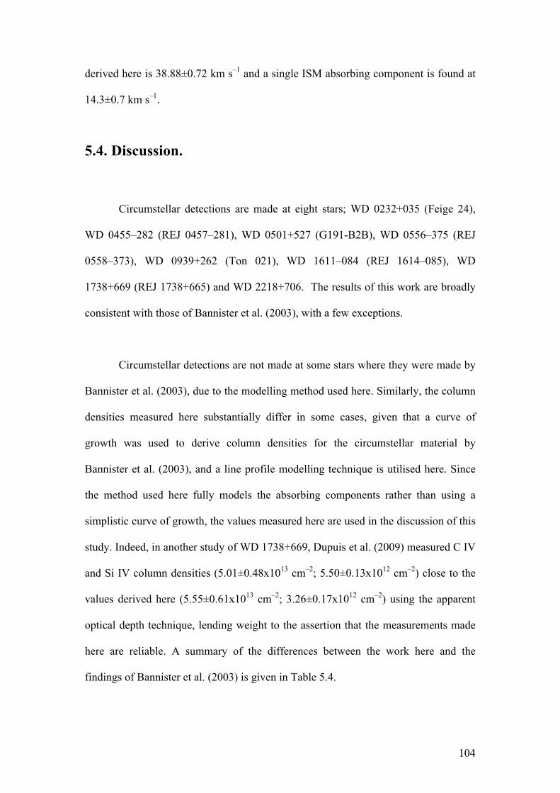
104
derived here is 38.88±0.72 km s–1 and a single ISM absorbing component is found at
14.3±0.7 km s–1.
5.4. Discussion.
Circumstellar detections are made at eight stars; WD 0232+035 (Feige 24),
WD 0455–282 (REJ 0457–281), WD 0501+527 (G191-B2B), WD 0556–375 (REJ
0558–373), WD 0939+262 (Ton 021), WD 1611–084 (REJ 1614–085), WD
1738+669 (REJ 1738+665) and WD 2218+706. The results of this work are broadly
consistent with those of Bannister et al. (2003), with a few exceptions.
Circumstellar detections are not made at some stars where they were made by
Bannister et al. (2003), due to the modelling method used here. Similarly, the column
densities measured here substantially differ in some cases, given that a curve of
growth was used to derive column densities for the circumstellar material by
Bannister et al. (2003), and a line profile modelling technique is utilised here. Since
the method used here fully models the absorbing components rather than using a
simplistic curve of growth, the values measured here are used in the discussion of this
study. Indeed, in another study of WD 1738+669, Dupuis et al. (2009) measured C IV
and Si IV column densities (5.01±0.48x1013 cm–2; 5.50±0.13x1012 cm–2) close to the
values derived here (5.55±0.61x1013 cm–2; 3.26±0.17x1012 cm–2) using the apparent
optical depth technique, lending weight to the assertion that the measurements made
here are reliable. A summary of the differences between the work here and the
findings of Bannister et al. (2003) is given in Table 5.4.

105
Table 5.4. The key differences between the findings of this study and that of
Bannister et al. (2003).
WD Key differences.
0050–335 Bannister et al. (2003) found two components in the coadded C IV
doublet; only absorbing one component is modelled here.
0455–282 The C IV column measured (3.32±6.6x1013 cm–2) differs to that
measured by Bannister et al. (2003; 1.82x1014 cm–2).
Column density measurements are presented here for the N V and Si IV
circumstellar components where they were not in the previous study.
0501+527 The C IV column measured (1.04±0.1x1014 cm–2) is greater than the
value stated by Bannister et al. (2003; 2.40x1013 cm–2).
0556–375 A C IV column density was measured here where it was not previously.
0948+534 A hint of circumstellar components to each of the high ion absorption
features is seen here for the first time, though their velocities were
inconsistent across absorption features and their addition to the line
profile models is not statistically significant.
1611–084 Bannister et al. (2003) found a C IV column density of 3.16x1013 cm–2,
whereas a column density of 9.77±1.9x1012 cm–2 is measured here.
A Si IV column density measurement is made here where it was not by
Bannister et al. (2003).
1738+669 No circumstellar N V is detected in this study.
The column C IV and Si IV densities here differ (5.55±0.61x1013 cm–2;
3.26±0.17x1012 cm–2) substantially to those measured by Bannister et
al. (2003; 1.70x1013 cm–2; 1.66x1013 cm–2).

106
Table 5.4 - continued
WD Key differences.
2152–548 Bannister et al. (2003) found two components in the coadded C IV
doublet; only absorbing one component is modelled here.
2218+706 The C IV and Si IV column densities measured here (1.19±0.17x10¹³
cm–2; 7.98±0.59x1013 cm–2) are somewhat different to those measured
by Bannister et al. (2003; 4.17x1013 cm–2; 4.07x1013 cm–2).
In this section, possible origins of the circumstellar absorption are explored,
with a summary presented in Section 5.5. Debris discs are discussed in 5.4.1, while
5.4.2 details whether ionisation of the ISM by the white dwarfs can explain the
observed circumstellar features. White dwarf mass loss is examined in 5.4.3 and PN
material is explored in 5.4.4.
5.4.1. Circumstellar discs.
The circumstellar discs at cooler white dwarfs are located a few tens of stellar
radii from their host stars. One would expect any solids in analogous circumstellar
discs at hotter stars to sublimate, given the proximity of such discs to the parent star
(e.g. von Hippel et al. 2007). A search for gaseous components to circumstellar discs
at hot white dwarfs by Burleigh et al. (2010, 2011), which included the work from the
previous chapter and further stars from the sample studied here, did not find any
evidence of gaseous disc emission. Furthermore, no infrared excesses were seen at
any of the stars included in this work in the surveys of Mullally et al. (2007) or Chu et

107
al. (2011). WD 2218+706 does harbour an infrared excess (M. Burleigh, priv. comm.),
although this may be due to the PN still present at the star. However, as discussed at
length in the previous chapter, a lack of confirmed circumstellar disc detections at
these stars does not completely rule out their presence.
Indeed, two white dwarfs (WD 0501+527 and WD 1611–084) have values of
vCSshift comparable to vgrav, suggesting that the absorbing circumstellar material may
be within a few tens of stellar radii of the star. Indeed, the vCS of WD 1611–084 is
well separated from both the detected ISM and predicted LISM velocities, possibly an
indication of circumstellar material. Furthermore, the vCS values at WD 0455–282,
WD 0556–375 and WD 0939+262 are slightly separate from the detected ISM
velocities along the sight lines to the stars. It may be the case, as suggested by
Lallement et al. (2011), that these objects are ionising circumstellar planetesimals or
material in a circumstellar disc. However, given how close vCS is to vLISM at these
objects, it is not immediately clear that these stars are not ionising an ISM cloudlet
loosely associated with the LISM; this is discussed in the next section. A key problem
with interpreting the observed absorption features is, as discussed by Gänsicke et al.
(2012), the debris accreted by cooler DZ stars is depleted of volatile elements, i.e.
carbon poor and silicate rich; the converse is true here, with strong carbon detections
and secondary silicon detections (and in some cases circumstellar nitrogen and
oxygen detections). Indeed, the one circumstellar high ion detection made in Gänsicke
et al.’s (2012) study was in the Si IV doublet only, lending weight to the argument
that if the material observed here were in a circumstellar disc, its origin is not the tidal
disruption of planets or asteroids.

108
The precise interaction of circumstellar discs with the intense radiation field to
a hot white dwarf is poorly understood. A model that predicts the details of the star-
disc interaction, and makes testable, quantifiable predictions is required.
5.4.2. Ionised ISM.
Given the inability of material inside the potential wells of the stars to explain
the observed circumstellar lines, another explanation is the ionisation of the ISM.
Indebetouw & Shull (2004) outlined possible reasons for the existence of high ions in
the ISM, including evaporating ISM cloudlets, planar conduction fronts, cooling
Galactic fountain material, the evaporation of hot gas in stellar wind and supernova
bubbles, turbulent mixing layers and white dwarf Strömgren spheres. If the high ion
absorption features observed in this work arise in ISM processes such as these, one
would expect such features to be seen along the lines of sight to both the white dwarfs
and nearby stars (except for the white dwarf Strömgren sphere model, where the
ionised material is local to the star). A search8 of IUE and HST STIS, GHRS and COS
data show no evidence of similar non-photospheric absorption in the C IV, N V, O V
or Si IV absorption lines in the spectra of objects along sight lines within five degrees
of the white dwarfs. This indicates that if ionisation of the ISM is occuring, it is in the
vicinity of the white dwarfs and not in an ISM process.
Since the study of Bannister et al. (2003), improvements have been made in
the mapping the morphology of the LISM (Redfield & Linsky, 2008). Using these
maps, the LISM cloud(s) traversing the line of sight to each white dwarf was
8 using the online tool at http://archive.stsci.edu/xcorr.php

109
identified and the projected velocity of each cloud calculated (Table 5.2, column six).
This allowed a comparison between both the detected ISM components and the
predicted LISM, and an examination of other (unresolved) ISM components related to
the LISM along each the sight line to each objects. Comparing vCSshift to the shift in
the predicted and observed ISM velocities shows the circumstellar and interstellar
velocities line up or are very close in many cases (Figure 5.6).
The photoionisation of the Hyades cloud by WD 0501+527 (at 50 pc) has
been used to explain both the similarity in high and low interstellar ion dynamical
properties (Redfield & Linsky 2008) and the high electron density (~0.5 cm–3) along
the sight line to the star (Redfield & Falcon 2008). Indeed, Tat & Terzian (1999)
found that WD 0501+527 has a Strömgren sphere that extends into the space within
20 pc of the Sun. Thus, the circumstellar absorption seen here is attributed to the
ionisation of the Hyades cloud. However, caution must be exercised; the metal
depletion along the sight line to the white dwarf is much higher than those along other
sight lines through the Hyades cloud. This may be evidence of multiple ISM
components along the sight line to this star, which are unresolved here. This has been
seen in other studies of the ISM; Welsh et al. (2010b) found that using high-resolution
observations, multiple component, complex absorption profiles can be seen where
only one absorber was detected in lower resolution data. In such cases, the velocities
all occupy a narrow range along the line of sight, around the LISM velocity. The LIC
does not extended beyond 13 pc along this sight line (Redfield & Falcon 2008),
constraining the distance to the detected secondary ISM component, which has a
velocity in keeping with vLIC.

110
At WD 1738+669 and WD 2218+706, vCS and vISM,pri match up well,
indicating that these stars may be ionising the ISM in their localities, causing the
observed absorption. These stars are too distant (at 243 and 436 pc) to be able to
ionise the LISM; indeed the projected LISM velocities (due to the LIC) are well
separated from vCS and vISM (vISM,pri at WD 2218+706). The secondary ISM
component detected in the spectrum of WD 2218+706 has a velocity in keeping with
vLIC, although the error on vISM,sec is large (4.01 km s–1).
At WD 0455–282, vCS (18.8±3.47 km s–1) is separate from both vISM
(12.1±1.5 km s–1) and vLISM (12.56±1.03 km s–1, due to the blue cloud). Given that
these velocities are, within errors, quite close, it may be that this star (at 108 pc) is
ionising some ISM in its Strömgren sphere that is loosely associated with the LISM,
and thus has a velocity similar to it. Similarly, the vCS at WD 0939+262
(9.38±6.6 km s–1) is far from vISM (–2.1±0.2 and –34.7±1.5 km s–1) and yet close to
vLIC (10.81±1.29 km s–1), suggesting that a ‘LIC like’ cloudlet may be being ionised.
The vCS, vISM,pri and vLISM values (10.2±1.07, 7.8±1.0 and 11.36±0.95 km s–1) at WD
0556–375 indicate an analogous situation may be present along the line of sight to the
DA. As well as a lack of high ion absorption features along nearby sight lines to these
stars, Welsh et al. (2010b) found no Na I absorption along sight lines near these stars
with velocities near vCS (although no data were present within ten degrees of WD
0939+262), indicating that whatever the source of the circumstellar high ions, they do
not arise in the nearby ISM.
The vCS detected in the spectra of WD 0232+035 and WD 1614–084 are well
separated from all detected and predicted ISM components, suggesting that the

111
ionisation of the ISM by these stars does not explain the observed circumstellar ions.
Other scenarios (such as the circumstellar discussion in Section 5.4.1, or the
ionisation of mass lost from the binary companion of WD 0232+035) may explain the
observations of these stars.
In addition to velocity data, column densities were measured for all
circumstellar and ISM detections. Indebetouw & Shull (2004) collated a table of
predicted C IV, N V, Si IV, and O VI column densities for the models considered in
their study. The column density ranges of only two models coincide with the column
densities seen here; the white dwarf Strömgren sphere model and the 4 M!
cooling
fountain (where hot, supernova heated gas rises to a 1 kpc scale height above the disc,
cools and falls back to the galactic plane; Shapiro & Field, 1976). However, the range
of column densities predicted by the 4 M!
cooling fountain covers only a small part
of the range of detected column densities, while the white dwarf Strömgren sphere
covers the full range of observed column densities.
The predicted metal column densities from the Strömgren sphere model in
Table 5.5 relate to a limited nH range. The full predicted column density ranges span
0.44x10¹² < Si IV < 4.4x1012 cm–2, 7.8x10¹² < C IV < 77x1012 cm–2,
1.2x10¹² < N V < 12x1012 cm–2 and 1.4x10¹² < O VI < 20x1012 cm–2 (Dupree and
Raymond, 1983). On an object-to-object basis, the predicted metal column densities
do not match those observed. However, when the limits of the range of expected

112
metal column densities are applied to the observed column densities, good agreement
is observed (Figure 5.7).
Several limitations exist in the model of Dupree & Raymond (1983). As noted
by Bannister et al. (2003), a single DA Strömgren sphere model with Teff = 60,000 K
was constructed; given that the range in Teff for the stars with circumstellar absorption
here is 38,840 - 69,711 K, one can expect significant variety in Strömgren radii (rS)
values when compared to the model, causing a variation in the expected column
density. Also, the model did not include photospheric metals, which act to reduce the
radiated stellar flux, reducing rS. This effect is more significant for Teff > 50,000 K,
when iron peak elements blanket the observed continuum (although the redistributed
flux may still contribute to the Strömgren sphere through lower energy transitions).
Seven of the eight stars with circumstellar absorption have Teff > 50,000 K, making
this omission a serious flaw in the physical model. The ISM was also assumed to be
isothermal (at 40,000 K) and of uniform density. For these reasons, the column
densities predicted should be treated as a rough estimate of scale, rather than precise
predictions.
Coupling the distances to the white dwarfs (Table 5.1) with rS estimates can
yield an estimate to the distance of the ionised material. Tat & Terzian (1999)
provided rS estimates for a variety of hot white dwarfs, for ne = 0.01 cm(3 and
0.03 cm(3. Using the rS values for the model star with the Teff closest to each of the
stars with circumstellar absorption, a series of rS estimates can be made for the DAs
here (Table 5.6).

113
Figure 5.6. A plot of vCSshift, with the shifts in the measured and predicted ISM
components (from Table 5.2). The measured velocity shifts are plotted in black, while
the predicted shifts in vLISM are plotted in grey. In some cases the error bars are
smaller than the plot symbols; the symbols are open to allow the error bars to be seen.

114
Table 5.5. The metal column densities for a range of ISM models (Table 1,
Indebetouw & Shull, 2004). All column densities are expressed in units of 1012 cm–2.
Model Si IV C IV N V O VI
Evaporating cloudlet* . . .
0.10 – 0.14
1.2 – 1.5
2.7 – 3.8
0.5 – 0.6
1.0 – 1.2
9 – 12
12 – 14
Planar Conduction
front*
0.10 – 0.16
0.029 – 0.097
1.6 – 3.2
0.89 – 2.7
0.6 – 1.0
0.40 – 1.0
8 – 10
6.7 – 14
Stellar wind bubble 0.21 – 0.25 3.3 – 4.0 1.3 – 1.6 21 – 25
SNR bubble* 0.4 – 0.6
~ 0.52
6.3 – 10
~ 7.8
3.2 – 5.0
~3.6
40 – 79
~47
Halo SNR bubble . . . 8 – 15 3.4 – 7.9 35 – 150
4M!
cooling 3.3 – 6.4 43 – 79 28 – 36 580 – 600
40 pc cooling cloud ~ 25 ~ 50 ~ 13 ~ 200
Turbulent mixing
layer 0.0010 – 0.47 0.025 – 6.8
0.0022 –
0.32 0.017 – 0.81
White dwarfs
(0.1<nH<1 cm–2)† 1.4 – 4.4 25 – 77 3.7 – 12 5.6 – 20
*the different rows correspond to different models references; †from Dupree &
Raymond (1983).
115
Figure 5.7. The column densities measured in this study, with the column density
ranges predicted by Dupree & Raymond (1983) for a DA Strömgren sphere (dashed
lines).

116
Table 5.6. The estimated rS (from Tat & Terzian, 1999) for each of the DAs with
circumstellar absorption, and estimated distances (D) to the absorbing material (for
ne = 0.01 and 0.03 cm(3). D was calculated by subtracting rS from the distance to
the star (from Table 5.1). The ISM component with a velocity matching vCS is
stated; a ‘?’ denotes the tentative association with the Hyades cloud. All rS and D
values are expressed in pc.
ne = 0.01 cm–3 ne = 0.03 cm–3 Star
rS D rS D ISM component
WD 0232+035a 33.66 44.34 16.18 61.82
WD 0455–282b 26.00 82 12.50 95.5
WD 0501+527b 26.00 24 12.50 37.5 ISM, pri (Hyades?)
WD 0556–375a 33.66 261.34 16.18 278.82
WD 0939+262c 39 178 18.86 198.14
WD 1611–084d 18.43 67.57 8.86 77.14
WD 1738+665c 39 204 18.86 224.14 ISM, pri
WD 2218+706b 33.66 402.34 16.18 419.82 ISM, pri
Note: the rS values adopted here were those calculated for the star with the nearest
Teff by Tat & Terzian 1999 to the star in question here, and are signified as follows:
aWD 0501+527 (Teff = 61 160 K); bWD 0232+035 (Teff = 50 000 K); cWD
1211+332 (Teff = 70 000 K); dWD 2111+498 (Teff = 39 800 K).
In the absence of consistent ISM components, the distances represent the distance
to the boundary of the Strömgren sphere.
Again, these rS estimates were made in the presence of several
oversimplifications similar to those already discussed; the basic formalism of

117
Strömgren (1939) was used, with an isothermal ISM at 7,500 K and discreet ne
values. A more thorough approach to estimating rS for the stars in this sample would
be to fully model the interaction of the stellar flux (taking proper account of UV
photospheric metal absorption) with the LISM (using measured ISM temperatures and
electron densities).
The study of the relationship of vCSshift and Teff by Lallement et al. (2011) using
the three DAs in their sample, as well as the samples of Holberg et al. (1998),
Bannister et al. (2003) and Barstow et al. (2010), reported considerable spread around
a trend of decreasing vCSshift with Teff. This was put down to the inclusion of a variety
of white dwarf environments, such as PN and binary systems. The variation in
photospheric and ISM component velocities along the sight lines to the stars here
offers another explanation for the observed dispersion in vCSshift.
This clearly demonstrates the importance of the white dwarf circumstellar
environment to our understanding of the ISM, and the need for a detailed analysis of
the spectra of hot white dwarfs in which ‘circumstellar’ high ions are seen, to
ascertain the true origin of these absorption features.
5.4.3. White dwarf mass loss.
A possible source for the observed circumstellar absorption put forward by
previous authors (e.g. Holberg et al. 1998, 1999; Bannister et al. 2003) is hot white
dwarf mass loss. Using the mass loss theory of Abbott (1982), Bannister et al. (2003)
found that the stars without circumstellar absorption had a decreasing mass loss rate
118
with decreasing Teff, while the stars with circumstellar absorption did not follow this
decay, concluding that mass loss played some part in the presence of the circumstellar
absorption features.
Since the calculations of Bannister et al. (2003), the metal abundances of the
stars in the sample have been revised (Barstow et al. 2012, in preparation; Chapter 3
of the thesis). In light of this, the mass loss calculations of Bannister et al. (2003) are
repeated here, to check whether a relationship between mass loss rate and
circumstellar features persists when the updated photospheric metal abundances are
considered. The formalism of Abbott (1982) provides a mass loss rate ( ), given a
stellar metallicity (relative to solar abundances; Z) and luminosity (L), using
The metallicity of each star is calculated using
where A*(z) is the abundance of the element with the atomic number z relative to
hydrogen (A!
(z) is the solar abundance of the metal). The metal abundances used in
the calculations are detailed in Appendix A and the stellar luminosities are stated in
Table 6.1.
!
˙ M

119
When the mass loss rates computed by Bannister et al. (2003) are compared to
the mass loss rate calculated here, a few differences emerge (Figure 5.8). The mass
loss rates for WD 0050–335, WD 1029+537 and WD 1611–084 are revised down
significantly, due to their greatly reduced N V abundances (see Chapter 3). WD
0050–335, having been moved to the non-circumstellar population, does not look out
of place with its new mass loss rate. Given the lower mass loss rate of WD 1611–084,
the pattern identified by Bannister et al. (2003) of the white dwarfs with circumstellar
absorption having high mass loss rates is broken. Indeed, the strongest determinant of
mass loss rate calculated by the formalism of Abbott (1982) is Teff, and the star with
the highest mass loss rate (WD 0621–376) does not display circumstellar features.
While the Abbott (1982) mass loss calculation method was used by Bannister
et al. (2003), and is repeated here to allow a comparison to their results, several
limitations exist in its application to hot white dwarfs. As discussed by Bannister et al.
(2003), this formalism was developed for the stellar envelopes of O-G type stars, and
is found to be most applicable to OB stars. Being concerned with main sequence stars,
the theory does not explain the mass-loss of Wolf-Rayet stars, which have a different
stellar structure to main sequence stars. Since white dwarfs are also structured
somewhat differently to main sequence stars, this casts doubt on the applicability of
this theory to white dwarfs.

120
Figure 5.8. A comparison of the mass loss calculations performed here using the
metal abundances in Appendix A (circles) to those of Bannister et al. (2003; squares).
The stars without circumstellar absorption lines are the filled symbols, while the stars
with circumstellar absorption are plotted with open symbols. The stars are plotted
from left to right in order of decreasing Teff to show the trend seen by Bannister et al.
(2003).

121
The formula of Abbott (1982) is based on the parameterisation of the
dependence of the radiative force on the wind optical depth, which is only valid in a
limited range, and predicts an increasing radiative force with decreasing wind density.
However, this force will saturate (at a point depending on the metallicity of the
material; Kudritzki, 2002); this is not included in the Abbott (1982) model. Therefore,
the formalism always predicts a non-zero mass loss, even for compact stars such as
white dwarfs where at some point the radiative force will not be able to overcome the
gravity of the star.
More recent studies of hot white dwarf mass loss show that for
25,000 K ) Teff ) 50,000 K, no winds can exist for a star with log g > 7.0 and a solar
or sub-solar metallicity, since the radiative acceleration saturates below the
gravitational acceleration of the star (Unglaub, 2008). Similarly, a steady mass loss
cannot be sustained for a DA with Teff = 60,000 K and log g > 7.0 (Unglaub, 2007).
Given that the lowest log g of any of the white dwarfs with circumstellar absorption is
7.05 (WD 2218+706), it can reasonably be concluded that mass loss does not account
for the observed circumstellar lines in the spectra of WD 0455–282, WD 0501+527,
WD 0556–375, WD 1611–084 and WD 2218+706, given that the Teff values of these
stars are all lower than 60,000 K. The remaining white dwarfs (WD 0232+035, WD
0939+262 and WD 1738+669) do not have Teff values much greater than 60,000 K.
No rigorous mass loss calculations have been made for Teff > 60,000 K,
although it seems unlikely mass loss can exist in these hotter DAs. In thin winds, the
majority of the radiative force comes from the CNO elements (Vink et al. 2001).
When more and more particles of these elements change into the helium like

122
ionisation stage at higher Teff, the radiative force is reduced, since the lines of this
ionisation stage are at very short wavelengths away from the flux maximum. Thus, it
is not immediately clear that winds are more likely to exist in DA stars with
Teff > 60,000 K, despite their higher luminosity.
If any winds were to be present at all, they would consist only of metals since
hydrogen would be in hydrostatic equilibrium. Following the arguments of Seaton
(1996), initial estimates for a DA with Teff = 66,000 K and log g = 7.7 suggest that the
outward flow of CNO elements in an otherwise hydrostatic atmosphere cannot exceed
a rate of the order 10–19 M!
yr–1 (Unglaub, priv. comm.). Indeed, a mass loss rate
much higher would rapidly empty the white dwarf atmosphere of CNO elements. If
mass loss were to occur, the winds must have a velocity of the order of a few
thousand km s-1, since that is roughly the escape velocity of a white dwarf. In the case
of sdB stars, mass loss occurs at a rate of the order 10–11 M!
yr–1, and the metallic
winds are accelerated up to several thousands of km s–1, exceeding the escape velocity
of the star (Votruba et al. 2010). No circumstellar absorption features like those
studied here have been reported. Though no calculations have been performed
detailing the mass loss rates required to produce such circumstellar absorption, it
could be argued that even if such winds were to exist at the hottest white dwarfs with
circumstellar absorption, the combination of a low mass loss rate and high wind
velocity would cause a thin wind to be present, which is unlikely to account for the
observed absorption features since they are not seen in sdB stars with higher mass
loss rates and similar wind velocities.

123
5.4.4. Planetary nebula material.
Since one of the stars (WD 2218+706) with circumstellar absorption in its
spectrum is a bona fide CSPN, the possible link between ancient, diffuse CSPN and
circumstellar UV absorption is again examined. Following the methodology of
Bannister et al. (2003), the vphot–vCS values for the white dwarfs found here are plotted
with the planetary nebula expansion velocities of Napiwotzki & Schönberner (1995;
Figure 5.9).
Given the broad consistency between the velocities measured here with those
measured by Bannister et al. (2003), it is perhaps not surprising that this line of
analysis produced similar results. Again, the vphot–vCS for WD 2218+706 is
inconsistent with the expansion velocity of the PN at the star. The interpretation of
Bannister et al. (2003) was that the non–photospheric absorption seen at this star is
not located inside the expanding PN, but that the PN was a possible source of
material. Bannister et al. (2003) also suggested that the suspected PN at WD
1738+669 might also account for the observed circumstellar absorption.
Since the study of Bannister et al. (2003), however, evidence has emerged that
WD 1738+669 is not a CSPN, and the material associated with it is ionised ISM
inside the Strömgren sphere of the star (Frew & Parker, 2006). At WD 1738+669, vCS
matches vISM,pri; a similar situation exists at WD 2218+706. Given this, and that the
material at WD 1738+669 is now thought not to be related to an ancient PN, further
strength is given to the argument that the material seen at WD 2218+706 is not
contained within the PN at the star and it is in fact ionised material inside the white

124
dwarf Strömgren sphere. Whether the material was once resident in the PN and has
now become part of the ISM, or whether the ionised ISM is from another source,
cannot be determined from this study alone.
Figure 5.9. A comparison of the vphot – vCS values here (triangles) to the vexp
measurements from Napiwotzki & Schönberner (1995; circles). Since no nebula
radius measurements exist for the stars in this sample, the vphot – vCS values are plotted
at zero pc. Overlapping values are offset for clarity, and the values for WD 2218+706
are labelled.

125
Given the highly complex, localised structures seen in high-resolution
observations of PNe such as the Helix Nebula (Figure 1.4). It may be that highly
localised, thus far undetected, PN remnant structures lie along the sight lines to these
hot DAs, providing the observed absorption. A detailed investigation of this scenario
will form the basis of future work.
5.5. Summary.
• Circumstellar features have previously been seen at eight hot DA white
dwarfs, with two further possible cases reported. Given the recent
advancements made in the study of circumstellar discs at cooler white dwarfs,
the morphology of the ISM and hot white dwarf mass loss it is desirable to
better understand the source of this material.
• The material was measured using a technique that, for the first time, provided
column densities for all non-photospheric absorption features, rather than
providing a curve of growth for a few discreet absorption line b values for
most circumstellar features. Unambiguous signatures of circumstellar
absorption were again detected at eight stars.
• Several physical scenarios from which the material could originate were
discussed, including circumstellar discs, the ionisation of the ISM near the
stars, stellar mass loss and ancient PNe.

126
• If circumstellar discs are present at a few tens of stellar radii, it is reasonable
to assume they would not persist as solids. However, no signs of gas discs
have been found at the stars, although accretion is required at some of the
white dwarfs to explain their photospheric abundances. While such discs have
not been detected, the results here do not rule out their presence. The
differences between vCS and the measured and projected ISM velocities may
be explained by the ionisation of circumstellar material that is not associated
with the ISM. Indeed, the vCS detected at WD 1611–084 is far from all ISM
components. However, it is unlikely that any circumstellar discs present would
be due to the tidal disruption of planets or asteroids, given the ubiquitous C IV
detections.
• The circumstellar absorption seen at WD 0501+527 has been attributed to the
photoionisation of the Hyades cloud by the intense UV radiation of the star, in
keeping with other studies. The ionisation of the ISM by WD 1738+669 and
WD 2218+706 may explain the circumstellar absorption, given the agreement
in vCS and vISM,pri at these stars (vISM at WD 1738+669). Some difficulty is met
when linking the circumstellar absorption at WD 0455–282, WD 0556–375
and WD 0939+262, where vCS does not match up well with the detected ISM
components. It may be the case, given the distances to the stars and the
similarity in vCS and vLISM, that currently unresolved ISM cloudlets with
velocities near vLISM are being ionised.
• The range of measured circumstellar column densities are consistent with the
range of column densities predicted by hot white dwarf Strömgren sphere

127
models. Although the observed vCS of WD 0232+035 is inconsistent with both
measured and predicted ISM velocities along the sight line to the star, the
Strömgren radius is estimated to be of the order of 16–33 pc. The ionisation of
mass lost from the dwarf companion to this star could account for the
observed circumstellar features.
• The mass loss calculations made by Bannister et al. (2003) were repeated with
more up to date stellar metal abundances, and the relationship previously seen
between mass loss and circumstellar features no longer holds. Indeed, the
method used by Bannister et al. (2003) has since been found to be
inappropriate for hot DA stars. More recent studies show that mass loss cannot
occur for DAs with Teff < 60,000 K, and is unlikely to occur in sufficient
quantities to explain the observed circumstellar features in hotter stars, if at all.
• The circumstellar absorption at the CSPN WD 2218+706 is again found not to
share the PN expansion velocity. Studies since that of Bannister et al. (2003)
have found the ionised gas around WD 1738+669 is not from a PN but is
instead ionised ISM inside the white dwarf Strömgren sphere. This suggests
that the circumstellar features observed at theses stars are again ionised ISM
inside the Strömgren spheres of the star, though a localised structure left from
the PN phase may also be present.
• This study indicates that the origin of the observed circumstellar absorption
may be the ionisation of material inside the white dwarf Strömgren spheres.

128
This highlights the great influence the radiation field of white dwarfs has over
the nearby space, and contributes to our understanding of the ionised ISM.
• Alternatively, the circumstellar material observed may be due to the ionisation
of circumstellar discs/planetesimals. A model that details testable predictions
that can be compared to these observations will be insightful, and offer an
understanding of the evolution of extrasolar planetary systems through the hot
white dwarf phase.
• Higher resolution observations of the ISM along the sight lines to the stars will
allow a better charaterisation of any as yet unresolved interstellar cloudlets.
More realistic models of the Strömgren spheres of hot white dwarfs, that
account properly for the properties of the ISM near the stars, is needed, as is a
model of the interaction of circumstellar material with hot DA stars.

129
Chapter 6.
Conclusions and suggestions for further
work.
6.1. Introduction.
This chapter, the final in this thesis, pulls together the results of the previous
three science studies. A brief statement of the findings of each investigation is given,
followed by a discussion of how these results help to further shape our understanding
of white dwarf stars. Suggestions for future work that can extend the findings of this
study and improve our understanding of these fascinating objects are made.
6.2. Concluding remarks and suggestions for further work.
The first science chapter of this work deals with the controversy over whether
the nitrogen in the stars WD 0050–335, WD 1029+537 and WD 1611–084 can be
modelled with homogeneous nitrogen distributions, with abundances not inconsistent
with those of DAs with higher Teff, or whether higher abundance, stratified nitrogen
configurations are required. The observations of these stars are found to be well
explained by homogeneous models. A degeneracy is observed, where two minima are

130
present in the nitrogen model
!"2 distribution of WD 0050–335 and WD 1029+537,
near the two abundances previously reported for these stars. In each of these stars, the
lower abundance model has a global
!"2 minimum that was well separated (>3&) from
the secondary minimum. In WD 1611–084, the minima are less easy to disentangle.
The model line profiles for the best fitting abundance do not reproduce the observed
data well, and the lower abundance, homogeneous model is adopted as the best fit,
since this is the case at the other stars. A comparison of the abundances derived here
show that they are much closer to the predictions of Chayer et al. (1995) than
previous measurements.
A search was carried out for signatures of circumstellar gas discs in a sample
of eight white dwarfs, which have enhanced metal abundances when compared to
theoretical predictions. At none of these stars is any metal line emission observed. In
other studies, no infrared excesses were seen at any of the stars.
The final research chapter contains a re-analysis of a sample of 23 hot white
dwarfs, of which eight had previously been found to exhibit non-photospheric high
ion absorption features, with two further marginal detections. Circumstellar
absorption is measured at the eight objects where it has been seen previously and, for
the first time, proper modelling of the circumstellar absorption lines allowed column
densities to be derived for all circumstellar absorption features.
Four possible scenarios for the origin of this material were examined. Mass
loss is found not be significant at these stars, if it occurs at all, and thus is not thought
to be the cause of the circumstellar absorption. No firm evidence that ancient

131
planetary nebula are the origin of the material is found, as only one of the objects
(WD 2218+706) is a CSPN, and the observed velocity of the circumstellar material at
that star is inconsistent with measurements of the PN expansion velocity. This may,
however, be an oversimplification, since the morphology of planetary nebulae can be
highly inhomogeneous with extremely localised structures (such as those seen in the
HST image of the Helix Nebula; Figure 1.4). It may be the case that the circumstellar
absorption observed is due to some highly localised material left over from the PN
that would have been around the white dwarfs earlier in their lives. A more detailed
investigation of this will be the subject of future work.
While no evidence of circumstellar discs has been found at the stars, and the
precise behaviour of a circumstellar disc at such hot white dwarfs is poorly
understood, the observations do not allow their dismissal; the circumstellar velocity
shifts in two of the stars are in keeping with the gravitational redshifts expected at the
objects, while at the other DAs (except WD 1611–084) all of the circumstellar
velocity shifts are blue shifted with respect to the photosphere, as may be expected
were the material in a disc about the star. Furthermore, the vCS detected at three other
stars (WD 0455–282, WD 0556–375 and WD 0939+262) do not align exactly with
the measured ISM component velocities, suggesting that the circumstellar material
may be due to the ionisation of planetesimals near the stars, or circumstellar discs.
The characteristics of the circumstellar material detected at WD 0501+527 are
in keeping with what would be expected if this star were ionising the Hyades cloud.
The vCS at WD 0455–282, WD 0556–375 and WD 0939+262 are near the projected
vLISM values along the sight lines to the stars. This suggests, that instead of the

132
ionisation of circumstellar material, these stars may be ionising material associated
with the LISM. These stars, with distances ranging from 108 – 295 pc, are too distant
to be able to ionise the LISM. However, it could be the case that ISM cloudlets along
the sight lines to the stars with velocities near that of the LISM are being ionised.
Indeed, Welsh et al. (2010b) found that when re-observed with high-resolution
instruments, multiple absorbing components can be detected where single ISM
components were previously seen in lower resolution data.
This suggests that the UV flux of the stars may be ionising the nearby ISM,
forming a Strömgren sphere type structure. Estimates of the radii of these spheres
shows that the binary companion of WD 0232+035 sits well inside this ionisation
sphere, and the mass lost from the dwarf companion may be being ionised by the DA.
The column densities of the observed circumstellar absorption features are consistent
with the predictions of Dupree & Raymond (1983), for a DA Strömgren sphere.
However, this model contains several limiting assumptions, and needs to be
recalculated, taking proper account of the effect of photospheric metals, NLTE effects
and local ISM temperatures and densities.
While the finding that the nitrogen in WD 0050–335, WD 1029+537 and WD
1614–084 can be modelled homogeneously closes a minor controversy, the
application of this result to our understanding of circumstellar absorption at hot white
dwarfs is interesting. A link between the previously measured, anomalously high
metal abundances was previously made to the observed circumstellar absorption at
WD 1611–084, and the possible circumstellar absorption at WD 0050–335 (e.g.
Bannister et al. 2003). This work shows that such a link can no longer be claimed,

133
since the abundances measured here are not as exotic as was once thought. Indeed, the
previously accepted, high metal abundances of these stars caused Bannister et al.
(2003) to calculate high mass loss rates for these stars, giving the impression that the
stars with circumstellar material all have high mass loss rates; this is not seen in this
work.
The examination both of the sample of eight white dwarfs in Chapter 4 and the
23 stars in Chapter 5 throw up some interesting points. The objects observed in
Chapter 4 were selected based on their photospheric metal abundances. Chayer &
Dupuis (2010) and Dupuis, Chayer & Hénault-Brunet (2010) have reported that,
based on radiative levitation calculations and the observed photospheric abundances,
accretion is occurring at some of the stars that feature in this thesis. The source of this
accretion has not yet been determined, although many studies of the accretion of
material at cooler stars suggest that tidally disrupted asteroids and minor planets
provide the circumstellar discs detected in the infrared. Were such discs to be found at
hotter white dwarfs, it would provide valuable information on how extra solar
planetary systems evolve while the white dwarf is young and hot.
The higher temperature of such stars may inhibit the presence of such discs
close to the stars, and as the star cools, the disc may be able to persist at ever-closer
radii. Detailed models of the evolution and configuration of circumstellar discs at the
hotter stars are not available as yet, and would be an interesting avenue of study. Such
models may provide quantitative estimates of observables that could be searched for,
and allow the detection and charaterisation of circumstellar discs at the hotter DA
stars.

134
This study of circumstellar absorption at hot white dwarfs suggests that a link
between the observed features and the ISM may in fact be present. If at least some of
the observed high ions are due to ionisation from hot white dwarfs, then conclusions
drawn about the morphology and ionisiation of the ISM are at least in part incorrect.
Therefore, a thorough further study of all observed, non-photospheric high ions at hot
white dwarfs is necessary, to ascertain whether such high ions could be due to the
ionisation of the ISM in the locality of the hot white dwarfs. The size of the sample
here, with a mere eight stars showing circumstellar absorption, needs to be enlarged to
allow more confident conclusions to be drawn; indeed it is difficult to understand the
origin of the circumstellar absorption at the eight DAs studied here when the three
possible sources of circumstellar material (circumstellar discs, ionised ISM and binary
mass loss), or a combination of sources, can be inferred. The observation of more hot
DA stars with UV instruments such as STIS and COS may allow the further
identification of circumstellar absorption of hot DAs, allowing a more statistically
meaningful sample to be constructed. The re-observation of stars where accretion is
required to explain the observed photospheric abundances at higher resolution may
allow further circumstellar detections to be made, and will provide a source of the
necessary, accreted material.
The applications of this work to our understanding of the morphology of the
ISM have been discussed in detail. In 2013, the GAIA observatory is due to launch,
and it will map the positions and parallaxes of over a billion stars to an accuracy of
25#”. Given the relative faintness of the white dwarfs studied here, accurate
parallaxes are often difficult to measure. However, GAIA’s limiting magnitude (20) is

135
sufficiently high enough to allow positions and parallaxes all of the stars here to be
measured. When coupled with the better measurements for all other stars, more
detailed maps of the ISM structure can be obtained. This will allow a more thorough
understanding of how the hot white dwarfs studied here interact with the ISM.
WD 0948+534 remains an enigmatic object. Although preliminary
calculations by Barstow et al. (2003b) suggested that stratified, highly abundant
photospheric metals may account for the extremely narrow, highly absorbed metal
line profiles, this work shows this is not the case. A possible source of the observed
line profiles is a previously unaccounted for physical affect that becomes significant
for high Teff; WD 0948+534 (at 110,000 K) is significantly hotter than the next hottest
DA examined in this context (WD 1029+537, Teff = 44,350 K). Investigations into
the behaviour of model ions and the ionisation of metals in this high temperature
regime will no doubt provide another useful avenue of exploration. Alternatively, a
possible secondary component has been seen in the absorption features of the star
(Section 5.3.3.3.), and the centroids of the high ions (when fit with one component)
are inconsistent with one another, suggesting that the absorption features may be
contaminated by another source of high ion absorption along the sight line to the star.
Observations at higher resolution may allow the separation of these components, if
they are present, and finally determine the mechanism that provides the observed
absorption line profiles.
Similarly, the photospheric metal abundance measurements detailed by
Barstow et al. (2003b) modelled the complete absorption line profiles, including both
the photospheric and circumstellar absorption. The complete charaterisation of the

136
circumstellar absorbing components provided here allows the circumstellar
contribution to the high ion metal lines to be accounted for in the line profile
modelling. Re-analysing the sample of Barstow et al. (2003b) in this context will
allow a better understanding of the patterns between metal abundance and Teff. This
worthwhile study will inform our understanding of how hot white dwarfs evolve, and
the new metal abundances will allow better estimates of Teff to be made, that can then
be applied to studies of white dwarf evolution, the initial-final mass relation and the
mass-radius relation. Given its proximity, WD 0501+527 is often used as a bench
mark hot white dwarf against which other hot DAs are compared; correctly knowing
the photospheric abundances of this star is important for all of the other hot white
dwarf studies that use the metal abundances of this star in the modelling of other
objects.
Indeed, the inconsistency between the Teff values obtained from the Balmer
and Lyman line series observed in hot white dwarfs (Barstow et al. 2003a; Good et al.
2004) may be due to uncertainties in the inclusion of metals in the stellar models.
Using the better metal abundance estimates, and the updated Stark broadening
modelling of Tremblay & Bergeron (2009), may allow this effect to be better
understood. The use of Lyman line Teff derivations for white dwarfs in binary systems
will benefit greatly from this, as will the mass-radius and initial-final mass relation
studies that use white dwarfs in binary systems.
All of these conclusions and suggestions for further investigation show that
the field of hot white dwarfs is very much alive, and worthy of considerable interest.
The application of this further work to our understanding of the ultimate fate of the

137
overwhelming majority of stars is clear, and from this we can gain a far greater
insight into how our Solar System will eventually expire. I greatly look forward to the
advances made in this field in the years to come, and playing a part in them.

138
Appendix A.
Chapter 6: Tables of DA and solar metal
abundances used for mass loss calculations.

139
Table A1. Hot white dwarf metal abundances.
Star C III* C IV* N IV† N V* O V* Si IV† P IV†
WD 0050–335 0 5.00x10⁻⁸ 1.00x10⁻⁸ 6.05x10⁻⁷,a 0 4.80x10⁻⁹
WD 0232+035 7.64x10⁻⁸ 4.00x10⁻⁷ 8.71x10⁻⁸ 1.60x10⁻⁷ 2.31x10⁻⁶ 6.34x10⁻⁸
WD 0455–282 0 4.00x10⁻⁸ 3.76x10⁻⁷ 1.60x10⁻⁷ 1.00x10⁻⁵ 3.00x10⁻⁸ 1.80x10⁻⁸
WD 0501+527 1.99x10⁻⁷ 4.00x10⁻⁷ 1.67x10⁻⁷ 1.60x10⁻⁷ 3.51x10⁻⁷ 8.65x10⁻⁷ 2.08x10⁻⁸
WD 0556–375 1.70x10⁻⁷ 4.00x10⁻⁷ 1.86x10⁻⁷ 2.89x10⁻⁶ 3.00x10⁻⁶
WD 0621–376 1.59x10⁻⁷ 4.00x10⁻⁷ 1.60x10⁻⁶ 1.60x10⁻⁷ 2.00x10⁻⁶ 7.50x10⁻⁷ 3.07x10⁻⁸
WD 0939+262 3.68x10⁻⁷ 1.71x10⁻⁷ 8.38x10⁻⁸ 1.21x10⁻⁷ 1.21x10⁻⁷
WD 1029+537 3.00x10⁻⁷ 1.60x10⁻⁷ 1.00x10⁻⁸ 2.20x10⁻⁷,a 1.20x10⁻⁷ 9.50x10⁻⁸
WD 1057+719 0 0 0
WD 1123+189 0
WD 1254+223 0 0 0 0 0
WD 1314+293 0 0
WD 1337+705 0 0 1.00x10⁻⁹ 0 0 2.4x10⁻⁷ 9.98x10⁻⁸
WD 1611–084 4.00x10⁻⁷ 1.00x10⁻⁷ 1.76x10⁻⁶,a 9.50x10⁻⁹
WD 1738+669 9.14x10⁻⁸ 1.34x10⁻⁷ 5.81x10⁻⁸ 4.84x10⁻⁷ 4.84x10⁻⁷
WD 2023+246 0 0 0 0 3.80x10⁻⁹
WD 2111+498 0 0 1.29x10⁻⁸ 0 0 2.80x10⁻⁶ 4.48x10⁻⁹
WD 2152–548 0 4.00x10⁻⁹ 1.00x10⁻⁸ 0 0 7.50x10⁻¹⁰ 2.01x10⁻⁹
WD 2211–495 1.00x10⁻⁷ 8.00x10⁻⁷ 3.04x10⁻⁷ 1.60x10⁻⁷ 2.40x10⁻⁶ 2.40x10⁻⁶ 6.07x10⁻⁹
WD 2218+706 1.59x10⁻⁷ 6.70x10⁻⁷ 2.72x10⁻⁷ 9.60x10⁻⁶ 1.93x10⁻⁶
WD 2309+105 0 3.01x10⁻⁸ 2.00x10⁻⁹ 1.60x10⁻⁷ 1.20x10⁻⁷ 2.15x10⁻⁹
WD 2331–475 8.00x10⁻⁸ 4.00x10⁻⁷ 1.60x10⁻⁸ 2.00x10⁻⁸ 7.10x10⁻⁷ 4.80x10⁻⁷ 3.05x10⁻⁸
*from Barstow et al. (2003b); †from Barstow et al. (in preparation); afrom Chapter 3
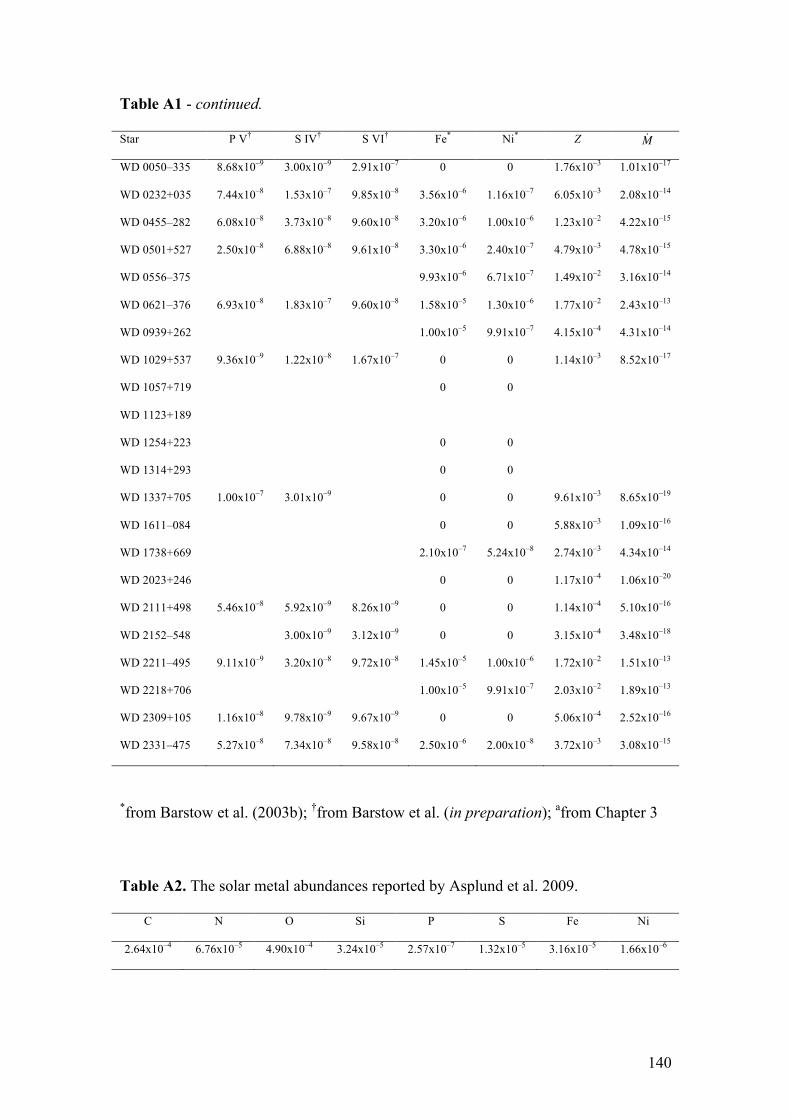
140
Table A1 - continued.
Star P V† S IV† S VI† Fe* Ni* Z
WD 0050–335 8.68x10⁻⁹ 3.00x10⁻⁹ 2.91x10⁻⁷ 0 0 1.76x10⁻³ 1.01x10⁻¹⁷
WD 0232+035 7.44x10⁻⁸ 1.53x10⁻⁷ 9.85x10⁻⁸ 3.56x10⁻⁶ 1.16x10⁻⁷ 6.05x10⁻³ 2.08x10⁻¹⁴
WD 0455–282 6.08x10⁻⁸ 3.73x10⁻⁸ 9.60x10⁻⁸ 3.20x10⁻⁶ 1.00x10⁻⁶ 1.23x10⁻² 4.22x10⁻¹⁵
WD 0501+527 2.50x10⁻⁸ 6.88x10⁻⁸ 9.61x10⁻⁸ 3.30x10⁻⁶ 2.40x10⁻⁷ 4.79x10⁻³ 4.78x10⁻¹⁵
WD 0556–375 9.93x10⁻⁶ 6.71x10⁻⁷ 1.49x10⁻² 3.16x10⁻¹⁴
WD 0621–376 6.93x10⁻⁸ 1.83x10⁻⁷ 9.60x10⁻⁸ 1.58x10⁻⁵ 1.30x10⁻⁶ 1.77x10⁻² 2.43x10⁻¹³
WD 0939+262 1.00x10⁻⁵ 9.91x10⁻⁷ 4.15x10⁻⁴ 4.31x10⁻¹⁴
WD 1029+537 9.36x10⁻⁹ 1.22x10⁻⁸ 1.67x10⁻⁷ 0 0 1.14x10⁻³ 8.52x10⁻¹⁷
WD 1057+719 0 0
WD 1123+189
WD 1254+223 0 0
WD 1314+293 0 0
WD 1337+705 1.00x10⁻⁷ 3.01x10⁻⁹ 0 0 9.61x10⁻³ 8.65x10⁻¹⁹
WD 1611–084 0 0 5.88x10⁻³ 1.09x10⁻¹⁶
WD 1738+669 2.10x10⁻⁷ 5.24x10⁻⁸ 2.74x10⁻³ 4.34x10⁻¹⁴
WD 2023+246 0 0 1.17x10⁻⁴ 1.06x10⁻²⁰
WD 2111+498 5.46x10⁻⁸ 5.92x10⁻⁹ 8.26x10⁻⁹ 0 0 1.14x10⁻⁴ 5.10x10⁻¹⁶
WD 2152–548 3.00x10⁻⁹ 3.12x10⁻⁹ 0 0 3.15x10⁻⁴ 3.48x10⁻¹⁸
WD 2211–495 9.11x10⁻⁹ 3.20x10⁻⁸ 9.72x10⁻⁸ 1.45x10⁻⁵ 1.00x10⁻⁶ 1.72x10⁻² 1.51x10⁻¹³
WD 2218+706 1.00x10⁻⁵ 9.91x10⁻⁷ 2.03x10⁻² 1.89x10⁻¹³
WD 2309+105 1.16x10⁻⁸ 9.78x10⁻⁹ 9.67x10⁻⁹ 0 0 5.06x10⁻⁴ 2.52x10⁻¹⁶
WD 2331–475 5.27x10⁻⁸ 7.34x10⁻⁸ 9.58x10⁻⁸ 2.50x10⁻⁶ 2.00x10⁻⁸ 3.72x10⁻³ 3.08x10⁻¹⁵
*from Barstow et al. (2003b); †from Barstow et al. (in preparation); afrom Chapter 3
Table A2. The solar metal abundances reported by Asplund et al. 2009.
C N O Si P S Fe Ni
2.64x10⁻⁴ 6.76x10⁻⁵ 4.90x10⁻⁴ 3.24x10⁻⁵ 2.57x10⁻⁷ 1.32x10⁻⁵ 3.16x10⁻⁵ 1.66x10⁻⁶
!
˙ M

141
Bibliography.
Aannestad P.A., Kenyon S.J., Hammond G.L., Sion E.M., 1993, AJ, 105, 1033
Abbott D.C., 1982, ApJ, 259, 282
Adams W.S., 1915, PASP, 27, 236
Arnaud K., 1996, ASPC, 101, 17
Asplund M., Grevesse N., Jacques Sauval A., Scott P., ARA&A, 47, 481
Bannister N. P., Barstow M. A., Holberg J. B., Bruhweiler F. C., 2003, MNRAS, 341,
477
Barstow M.A., Boyce D.D., Welsh B.Y., Lallement R., Barstow J.K., Forbes A.E.,
Preval S., 2010, ApJ, 723, 1762
Barstow M.A., Bond H.E., Holberg J.B., Burleigh M.R., Hubeny I., Koester D., 2005,
MNRAS, 362, 1134
Barstow M.A., Cruddace R.G., Kowalski M.P., Bannister N.P., Yentis D., Lapington
J.S., Tandy J.A., Hubeny I., Schuh S., Dreizler S., Barbee T.W., 2005, MNRAS, 362,
1273

142
Barstow M.A., Dobbie P., Holberg J.B, Hubeny I., Lanz T., 1997, MNRAS, 286, 58
Barstow M.A., Good S., Burleigh M., Hubeny I., Holberg J., Levan A., 2003a,
MNRAS, 344, 562
Barstow M.A., Good S.A., Holberg J.B., Hubeny I., Bannister N.P., Bruhweiler F.C.,
Burleigh M.R., Napiwotzki R., 2003b, MNRAS, 341, 870
Barstow M.A., Holberg J.B., Fleming T.A., Marsh M.C., Koester D., Wonnacott D.,
1994, MNRAS, 270, 499
Barstow M.A., Hubeny I., 1999, MNRAS, 299, 379
Barstow M.A., Hubeny I., Holberg J.B., 1998, MNRAS, 307, 884
Barstow M.A., Holberg J.B., Marsh M.C., Tweedy R.W., Burleigh M.R., Fleming
T.A., Koester D., Penny A.J., Sansom A., 1994b, MNRAS, 271, 175
Becklin E.E., Farihi J., Jura M., Song I., Weinberger A.J., Zuckerman B., 2005, ApJ,
632, 119
Bessel F.W., Herschel J.F.W., 1844, MNRAS, 6, 136
Bergeron P., Saffer R., Liebert J., 1992, ApJ, 432, 305

143
Bergeron P., Wesemael F., Lamontagne R., Fontaine G., Saffer R.A., Allard N.F.,
1995, ApJ, 449, 258
Bohlin R.C., Dickinson M.E., Calzetti D., 2001, AJ, 122, 2118
Bohlin R.C., Gordon K.D., Rieke G.H., Ardilla D., Carey S., Deustua S., Engelbracht
C., Ferguson H.C., 2011, AJ, 141, 173
Bond G., 1862, AN, 57, 131
Brinkworth C.S., Gänsicke B.T., Marsh T.R., Hoard D.W., Tappert C., 2009, ApJ,
696, 1402
Bruhweiler F.C., Kondo Y., 1983, ApJ, 269, 657
Burleigh M.R., Barstow M.A., Farihi J., Bannister N.P., Dickinson N.J., Steele P.R.,
Dobbie P.D., Faedi F., Gänsicke B.T., 2010, AIPC, 1273, 473
Burleigh M.R., Barstow M.A., Farihi J., Bannister N.P., Dickinson N.J., Steele P.R.,
Dobbie P.D., Faedi F., Gänsicke B.T., 2011, AIPC, 1331, 289
Casewell S., Dobbie P.D., Napiwotzki R., Burleigh M.R., Jameson R.F., 2009,
MNRAS, 395, 1795

144
Chayer P., Dupuis J., 2010, AIPC, 1273, 394
Chayer P., Fontaine G., Wesemael F., 1995, ApJS, 99, 189
Chayer P., Kruk J.W., Ake T.B., Dupree A.K., Malina R.F., Siegmund O.H.,
Sonneborn G., Ohl R.G., 2000, ApJ, 538, 91
Chayer P., Oliveira C., Dupuis J., Moos H.W., Welsh B.Y., 2006, ASPC, 348, 209
Chayer P., Vennes S, Dupuis J., 2005 ASPC, 334, 181
Chayer P., Vennes S., Pradhan A.K., Thejl P., Beauchamp A., Fontaine G., Wesemael
F., 1995, ApJ, 454, 429
Chiang E.I., Goldreich P., 1997, ApJ, 490, 368
Chu Y.H., Su K.Y.L., Bilikova J., Gruendl R.A., DeMarco O., Guerrero M., Updike
A.C., Volk K., Rauch T., 2011, AJ, 142, 75
Davidsson B.J.R., 1999, Icarus, 142, 525
Debes J.H., Sigurdsson S., 2002, ApJ, 572, 556
Debes J.H., Sigurdsson S., Hansen B., 2007, AJ, 134, 1662

145
Debes J.H., Hoard D.W., Wachter S., Leisawitz D.T., Cohen M., 2011, ApJS, 197, 38
Dreizler S., Werner K., 1993, A&A, 278, 199
Dreizler S., Wolff B., 1999, A&A, 348, 189
Dufour P., Liebert J., Fontaine G., Behara N., 2007a, Nature, 450, 522
Dufour P., Liebert J., Fontaine G., Behara N., 2007b, ASPC, 391, 241
Dufour P., Fontaine G., Liebert J., Schmidt G.D., Behara N., 2008, ApJ, 683, 978
Dufour P., Kilic M., Fontaine G., Bergeron P., Lachapelle F.R., Kleinmann S.J.,
Legget S.K., 2010, ApJ, 719, 803
Dupree A.K., Raymond J. C., 1982, ApJ, 263, 63
Dupree A.K., Raymond J.C., 1983, ApJ, 275, 71
Dupuis J., Chayer P., Hénault-Brunet V., 2010, AIPC, 1273, 412
Dupuis J., Chayer P., Hénault-Brunet V., Venes S., Kruk J.W., 2010, AAS, 215,
45205
Dupuis J., Chayer P., Vennes S., Christian D.J., Kruk J.W., 2000, ApJ, 537, 127

146
Dupuis J., Fontaine G., Wesemael F., 1993, ApJS, 87, 345
Dupuis J., Fontaine G., Pelletier C., Wesemael F., 1992, ApJS, 82, 505
Dupuis J., Fontaine G., Pelletier C., Wesemael F., 1993, ApJS, 84, 73
Dupuis J., Oliveira C.M., Hébrard G.H., Woos H.W., Sonnentrucker P., 2009, ApJ,
690, 1045
Eisenstein D.J., Liebert J., Koester D., Kleinmann S.J., Nitta A., Smith P.S., Barentine
J.C., Brewington H.J., Brinkmann J., Harvanek M., Krzesinski J., Neilsen E.H. Jr.,
Long D., Schneider D.P., Snedden S.A., 2006, AJ, 132, 676
Farihi J., Barstow M.A., Redfield S., Dufour P., Hambly N.C., 2010, MNRAS, 404,
2123
Farihi J., Jura M., Zuckerman B., 2009, ApJ, 694, 805
Farihi J., Zuckerman B., Becklin E.E., 2008, ApJ, 674, 431
Feldman P.D., Sahnow D.J., Kruk J.W., Murphy E.M., Moos H.W., 2001, JGR, 106,
8119
Fontaine G., Brassard P., 2005, ASPC, 627, 404

147
Fontaine G., Brassard P., Bergeron P., 2001, PASP, 113, 409
Fowler R.H., 1926, MNRAS, 87, 114
Frew D., Parker Q., 2006, IAUS, 234, 49
Frisch P.C., York D.G., 1983, ApJ, 271, L59
Gänsicke B.T., Koester D., Marsh T.R., Rebassa-Masergas A., Southworth J., 2008,
MNRAS, 391, L103
Gänsicke B.T., Marsh T.R., Southworth J., 2007, MNRAS, 380, L35
Gänsicke B.T., Marsh T.R., Southworth J., Rebassa-Masergas A., 2006, Science, 314,
1908
Good S., Barstow M., Holberg J., Sing D., Burleigh M., Dobbie P., 2004, MNRAS,
355, 1031
Graham J.R., Matthews K., Neugebauer G., Soifer B.T., 1990, ApJ, 357, 216
Greenstein J.L., 1960, In Stars and Stellar Systems, Vol 6, Stellar Atmospheres, ed.
J.L. Greenstein (Chicago: University of Chicago Press)
Hartmann S., Nagel T., Rauch T., Werner K., 2011, A&A, 530, 7

148
Herschel W., 1785, RSPT, 75, 40
Hoard D.W., Wachter S., Sturch L.K., Widhalm A.M., Weiler K.P., Pretorius M.L.,
Wellhouse J.W., Gibiansky M., 2007, AJ, 134, 26
Holberg J.B., Barstow M.A., Bruhweiler F.C, Collins J., 1996, AJ, 111, 2361
Holberg J.B., Barstow M.A., Bruhweiler F.C., Dobbie P.D., 1999b, ApJ, 517, 841.
Holberg J.B., Barstow M.A., Bruhweiler F.C., Hubeny I., 2000, BAAS, 197, 8304.
Holberg J.B., Barstow M.A., Bruhweiler F.C., Hubeny I., Green E.M., 1999a, ApJ,
517, 850
Holberg J.B., Barstow M.A., Bruhweiler F.C., Sion E., 1995, ApJ, 453, 313
Holberg J.B., Barstow M.A., Lanz T., Hubeny I., 1997, ApJ, 484, 871
Holberg J.B., Barstow M.A., Green E.M., 1997, ApJ, 474, 127
Holberg J.B., Barstow M.A., Sion E.M., 1998, ApJS, 119, 207
Holberg J.B., Barstow M.A., Sion E.M., 1999, ASPC, 169, 485

149
Holberg J. B., Bruhweiler F. C., Anderson J., 1995, ApJ, 443, 753
Holberg J.B., Oswalt T.D., Sion E.M., 2002, ApJ, 571, 512
Holberg J., Wesemael F., Wegner G., Bruhweiler F., 1985, ApJ, 484, 871
Horne K., Marsh T.R., 1986, MNRAS, 218, 761
Hubeny I., Hummer D.G., Lanz T., 1994, A&A, 262, 501
Hubeny I., Lanz T., 1992, A&A, 262, 501
Hubeny I., Lanz T., 1995, ApJ, 439, 875
Hubeny I., Lanz T., 2003, ASPC, 288, 51
Indebetouw R., Shull J.M., 2004a, ApJ, 605, 205
Indebetouw R., Shull J.M., 2004b, ApJ, 607, 309
Jordan S., Heber U., Engels D., Koester D., 1993 A&A, 273, 27
Jura M., 2003, ApJ, 584, 91
Jura M., 2003, ApJ, 653, 613
150
Jura M., 2008, AJ, 135, 1785
Jura M., Farihi J., Becklin E.E., 2007, ApJ, 663, 1285
Jura M., Farihi J., Zuckerman B., 2009, AJ, 137, 3191
Jura M., Muno M.P., Farihi J., Zuckerman B., 2009, ApJ, 699, 1473
Kahn S.M., Wesemael F., Liebert J., Raymond J.C., Steiner J.E., Shipman H.L., 1984,
ApJ, 278, 255
Kawka A., Vennes S., Dupuis J., Chayer P., Lanz T., 2008, ApJ, 675, 1518
Kilic M., Redfield S., 2007, ApJ, 660, 641
Kilic M., von Hippel T., Legget S.K., Winget D.E., 2005, ApJ, 632, 115
Kilic M., von Hippel T., Legget S.K., Winget D.E., 2006, ApJ, 646, 474
Kimble R.A., Woodgate B.E., Bowers C.W., Kraemer S.B., Kaiser M.E., Gul T.R.,
Heap S.R., Danks A.C., Boggess A., Green R.F., et al. 1998, ApJ, 492, 83
Klein B., Jura M., Koester D., Zuckerman B., 2011, ApJ, 741, 64

151
Kleinman S.J., Harris H.C., Eisenstein D.J., Liebert J., Nitta A., Krzesinski J., Munn
J.A., Dahn C.C. et al., 2004, ApJ, 607, 426
Koester D., 1989, ApJ, 342, 999
Koester D., Wilken D., 2006, A&A, 453, 1051
Kudritzki R.P., 2002, ApJ, 577, 389
Kuiper G.P., 1941, PASP, 53, 248
Lallement R., Ferlet R., Lagrange A. M., Lemonie M., Vidal-Madjar A., 1995, A&A,
304, 461
Lallement R., Welsh B.Y., Barstow M.A., Casewell S.L., 2011, A&A, 533, 140
Lanz T., Barstow M.A., Hubeny I., Holberg J.B., 1996, ApJ, 473, 1089
Lanz T., Hubeny I., 1995, ApJ, 439, 905
Lanz T., Hubeny I., 2003a, ASPC, 146, 417
Lanz T., Hubeny I., 2003a, ASPC, 288, 117
Laughlin G., Bodenheimer P., Adams F.C., 1997, ApJ, 482, 420

152
Liebert J., Bergeron P., Eisenstein D., Harris H.C., Kleinmann S.J., Nitta A.,
Krzesinski J., 2004, ApJL, 606, 147
Liebert J., Harris H.C., Dahn C.C., Schmidt G.D., et al., 2003, ApJ, 126, 2521
Liebert J., Young P.A., Arnett D., Holberg J.B., Williams K.A., 2005, ApJ, 630, 69
Luyten W.J., 1952, ApJ, 116, 283
MacDonald J., 1992, ApJ, 396, 619
Marsh M.C., 1995, PhD Thesis, University of Leicester
Marsh M.C., Barstow M.A., Buckley D.A., Burleigh M.R., Holberg J.B., Koester D.,
O’Donoghue D., Penny A.C., Sansom A.E., 1997, MNRAS, 286, 369
Maxted P.F.L., Marsh T.R., North R.C., 2000, MNRAS, 317, 41
McCook G.P., Sion E.M., 1999, ApJS, 121, 1
Meeting of the Royal Astronomical Society, 11th January 1935, in The Observatory,
1935, 58, 33

153
Melis C., Farihi J., Dufour P., Zuckerman B., Burgasser A.J., Bergeron P., Bochanski
J., Simcoe R., 2011, ApJ, 732, 90
Melis C., Jura M., Albert L., Klein B., Zuckerman B., 2010, ApJ, 722, 1078
Moos H.W., Cash W.C., Cowie L.L., Davidsen A.F., Dupree A.K., Feldman P.D.,
Friedman S.D., Green J.C., Green R.F., Gry C., et al. 2000, ApJ, 538, 1
Mullally F., Kilic M., Reach W.T., Kuchner M.J., von Hippel T., Burrows A., Winget
D.E., 2007, ApJS, 171, 206
Napiwotzki R., 1997, A&A, 322, 256
Napiwotzki R., Schönberner D., 1995, A&A, 301, 545
Napiwotzki R., Green P.J., Saffer R.A., 1999, ApJ, 517, 399
Napiwotzki R., 1999, A&A, 350, 101
Pelletier C., Fontaine G., Wesemael F., Michaud G., Wegner G., 1986, ApJ, 307, 242
Peters C.A.F., 1851, AN, 32, 1
Redfield S., Falcon R., 2008, ApJ, 683, 207

154
Redfield S., Linsky J.L., 2002, ApJS, 139, 439
Redfield S., Linsky J.L., 2004a, ApJ, 602, 776
Redfield S., Linsky J., 2004b, ApJ, 613, 104
Redfield S., Linsky J.L., 2008, ApJ, 673, 283
Renzini A., Voli M., 1981, A&A, 94, 175
Saffer R., Livio M., Yungelson L.R., 1998, ApJ, 502, 394
Sahu M.S., Landsman W., Bruhweiler F.C., Gull T.R., Bowers C.A., Lindler D.,
Feggans K., Barstow M.A., Hubeny I., Holberg J.B., 1999, ApJ, 523, 159
Sahnow D.J., Moos H.W., Ake T.B., Andersen J., Andersson B.-G., Andre M., Artis
D., Berman A.F., Bair W.P., Brownsberger K.R., et al., 2000, ApJ, 538, 7
Savage B.D., Lehner N., 2006 ApJS, 162, 134
Savage B.D., Sembach K.R., 1991, ApJ, 379, 245
Schatzmann E., 1958, White Dwarfs (Amsterdam: North Holland Publishing)
Schmidt G.D., Smith P.S., 1995, ApJ, 448, 305

155
Schönberg M., & Chandrasekhar S., 1942, ApJ, 96, 161
Schuh S., Barstow M.A., Dreizler S., 2005, ASPC, 334, 237
Schuh, S., Dreizler S., Wolff B., 2002, A&A, 382, 164
Seaton M., 1996, Ap&SS, 237, 107
Sfeir D.M., Lallement R., Crifo F., Welsh B.Y., 1999, A&A, 346, 785
Shaprio P.R., Field G.B., 1976, ApJ, 205, 762
Sion E.M., Bohlin R.C., Tweedy R.W., Vauclair G.P., 1992, ApJ, 391, 29
Sion E.M., Greenstein J.L., Landstreet J.D., Liebert J., Shipman H.L., Wegner G.A.,
1983, ApJ, 269, 253
Strömgren B., 1939, ApJ, 89, 526
Struve O., 1866, MNRAS, 26, 268
Su K.Y.L., Chu Y.-H., Rieke G.H., Huggins P.J., Gruendl R., Napiwotzki R., Rauch
T., Latter W.B., Volk K., 2007, ApJ, 657, 41
Tat H., Terzian Y., 1999, PASP, 111, 1258

156
Tremblay P.E. & Bergeron P, 2009, ApJ, 696, 1755
Tweedy R. W., Kwitter K. B., 1994, ApJ, 433, 93
Unglaub K., 2007, ASPC, 372, 201
Unglaub K., 2008, A&A, 486, 923
Unglaub K, Bues I., 2000, A&A, 359, 1042
Vallegra J., 1998, ApJ, 497, 921
Vallerga J., Vedder P., Craig N., Welsh B., 1993, ApJ, 411, 729
Van Maanen A., 1917, PASP, 29, 258
Vauclair G., Vauclair S., Greenstein J.L., 1979, A&A, 80, 79
Vennes S., Chayer P., Dupuis J., 2005, APJ, 622, L121
Vennes S., Chayer P., Dupuis J., Lanz T., 2006, ApJ, 652, 1554
Vennes S., Lanz T., 2001, ApJ, 553, 399
157
Vennes S., Pelletier C., Fontaine G., Wesemael F., 1988, ApJ, 331, 876
Vennes S., Thorstensen J.R., 1994, AJ, 108, 1881
Vink J., de Koeter A., Lamers H., 2001, A&A, 369, 574
von Hippel T., Kuchner M.J., Kilic M., Mullally F., Reach W.T., 2007, ApJ, 662, 544
Votruba V., Feldmeier A., Krticka J., Kubát J., 2010, Ap&SS, 329, 159
Weidemann V., 1987, A&A, 188, 74
Welsh B.Y., 1991, ApJ, 373, 556
Welsh B.Y., Lallement R., 2005, A&A, 436, 615
Welsh B.Y., Lallement R., 2010, PASP, 122, 1320
Welsh B.Y., Lallement R., Vergely J.-L., Raimond S., 2010a, A&A, 510, 54
Welsh B.Y., Wheatley J., Siegmund O.H.W., Lallement R., 2010b, ApJL, 712, 199
Welsh B.Y., Sfeir D., Sirk M., Lallement R., 1999, A&A, 352, 308
Welsh B.Y., Vallegra P.W., Vedder J.V., 1990, ApJ, 358, 473
158
Welsh B.Y., Wheatley J., Siegmund O.H.W., Lallement R., 2010, ApJL, 712, 199
Werner K., Rauch T., Kruk J.W., 2007, A&A, 466, 317
Wolff B., Koester D., Dreizler S., Haas S., 1998, A&A, 329, 1045
Wolff B., Kruk J.W., Koester D., Allard N.F., Ferlet R., Vidal-Madjar A., 2001 A&A,
373, 674
Wood M., 1992, ApJ, 386, 539
Wood M., 1995, LNP, 443, 41
Woodgate B.E., Kimble R.A., Bowers C.W., Kraemer S., Kaiser M.E., Danks A.C.,
Grady J.F., Loicaono J.J., Brumfield M., Feinberg L., et al. 1998, PASP, 110, 1183
Young P., Schneider D.P., Shectman S.A., 1981, ApJ, 245, 1035
Zuckerman B., Koester D., Dufour P., Melis C., Klein B., Jura M., 2011, ApJ, 739,
101
Zuckerman B., Koester D., Melis C., Hansen B.M., Jura M., 2007, ApJ, 671, 872
Zuckerman B., Koester D., Reid I.N., Hünsch M., 2003, ApJ, 596, 477

159
Zuckerman B, Reid I.N., 1998, ApJ, 505, 143


