
THE INVESTIGATION OF FLUID PROPERTIES AND SEISMIC ATTRIBUTES
FOR RESERVOIR CHARACTERIZATION
By
TERRA E. BULLOCH
A THESIS
Submitted in partial fulfillment of the requirements
for the degree of
MASTER OF SCIENCE IN GEOLOGICAL ENGINEERING
MICHIGAN TECHNOLOGICAL UNIVERSITY
1999

This thesis, “THE INVESTIGATION OF FLUID PROPERTIES AND SEISMIC
ATTRIBUTES FOR RESERVOIR CHARACTERIZATION”, is hereby approved in
partial fulfillment of the requirements for the Degree of MASTER OF SCIENCE IN
GEOLOGICAL ENGINEERING.
DEPARTMENT: Geological Engineering and Sciences
Signatures:
Thesis Advisor:____________________________________
Dr. Wayne D. Pennington
Department Chair:___________________________________
Dr. Theodore J. Bornhorst
Date:__________________________________ _

ABSTRACTSeismic data are used in petroleum exploration to define geologic features
in the subsurface. Recent advancements in seismic exploration have examined
the effect of fluid and rock properties on seismic attributes. These advancements
may provide improved reservoir characterization using techniques examined here.
This is accomplished two parts; first, a study of fluid properties and their effect on
seismic response; second, an attempt to relate the seismic attributes computed
from a 2-D seismic line to the fluids and the rock framework in a particular reser-
voir in Michigan.
To study the fluid properties and their seismic significance, a number of
published predictors are used to model reservoir data. The models used in this
study include the Batzle and Wang (1992) model to predict fluid properties, the
Gassmann-Biot model to predict rock velocities as a function of the saturating flu-
ids, and the amplitude variation with offset (AVO) model using Zoeppritz’ equa-
tions to predict seismic response from the layered rock properties.
The Batzle and Wang (1992) model results are compared to the Batzle and
Han (1997) laboratory data to establish the usefulness of the model as a predictor
of fluid properties and found to perform reasonably well, although the model
slightly underpredicts the velocity of live oils and overpredicts the velocity of dead
oils. As a result, this model can be used for specific reservoir cases.
The Batzle and Wang, Gassmann-Biot, and Zoeppritz models are applied
to a Gulf of Mexico field; the acoustic impedance and Poisson’s ratio are deter-
mined and it is shown that an AVO response is present as a result of the fluid and
rock properties. The modeling of Lobster Field illustrates the usefulness of predic-
tors described in this thesis for modeling the reservoir through time as it is pro-
duced and the pressure decreases.
In an effort to apply these concepts to actual seismic data, 2-D seismic
data from Crystal Field, Michigan was evaluated with the intention of identifying a
large amount of by-passed oil that has been left between many wells. As a means
for identifying by-passed oil, efforts were made to enhance seismic imaging of
i

faults or karstic features in Crystal Field based on seismic attributes. Karstification
and increased porosity or fracturing were not observable on the seismic data due
to acquisition parameters that limit the usefulness of the data in the shallow sec-
tion.
Data acquired for shallow horizons may be very useful for evaluating the
seismic attributes in other fields in the Michigan Basin if the fold and offset ranges
are appropriate. Good quality seismic data for the horizons of interest is neces-
sary to evaluate seismic attributes.
ii

ACKNOWLEDGMENTSFirst and foremost, I would like to thank GOD for all that I have been given.
I thank my husband, John, for his support and friendship. If it weren’t for him I
wouldn’t have made it this far. I thank my family for being there for me; especially
my mother, Barbara, for all of her support and long talks and my sister, Jennifer,
for being such a wonderful sister and friend. I thank my friend Lisa Stright for
being my exercise buddy and for keeping me going through all of those stressful
times with her motivation.
I thank my advisor, Wayne D. Pennington, for all of the guidance and oppor-
tunities he has provided me. I thank my committee: Jackie Huntoon, Jim Wood,
Randy McKnight, and Jaroslaw Drelich, for their time and input.
A special thank you to Randy McKnight for his mentoring while I was a
summer intern at Marathon Oil Company and his friendship since. I also thank
Randy for his many ideas and input for this work.
I thank all of my friends here at Michigan Tech that have given me support
and friendship throughout the years. A special thanks to Mike Dolan for his friend-
ship and all of his computer support. You are appreciated more than you know.
Many thanks to those that have helped with this work: Josh Haataja, Bill
Everham, Carol Asiala, Steve Chittick, Bill Harrison, Thomas Benz, and Dan
Brugeman.
I would like to acknowledge Marathon Oil Company and Texaco for provid-
ing the data for this work and thank them for their permission to publish it.
iii

I thank the following companies and organizations for their support of this
project through funding, data, and software that I have used throughout:
Marathon Oil Company
Texaco
Department of Energy:
Recovery of Bypassed oil in the Dundee formation of the MichiganBasin using Horizontal Drains, Contract # DE-FC22-94BC14983(PI: J.R. Wood)
Calibration of Seismic Attributes for Reservoir Characterization,Contract # DE-AC26-98BC15135 (PI: W.D. Pennington)
Advanced Characterization of Fractured Reservoirs in Shallow ShelfCarbonate Rocks: The Michigan Basin, Contract # DE-AC26-98BC15100 (PI: J.R. Wood)
Michigan Basin Geological Society (MBGS)
Society of Professional Well Log Analysts (SPWLA)
Schlumberger GeoQuest
Mercury International - iXL
Seismic Unix (CSM)
GeoGraphix
Cronus Development (Terra Energy)
Maness Petroleum
Aangstrom Precision
iv

TABLE OF CONTENTS
SECTION PAGE
ABSTRACT. . . . . . . . . . . . . . . . . . . . . . . . . . . . . . . . . . . . . . . . . . . . . . . . . . . . . . .i
ACKNOWLEDGMENTS . . . . . . . . . . . . . . . . . . . . . . . . . . . . . . . . . . . . . . . . . . . . iii
LIST OF FIGURES . . . . . . . . . . . . . . . . . . . . . . . . . . . . . . . . . . . . . . . . . . . . . . . vii
LIST OF TABLES . . . . . . . . . . . . . . . . . . . . . . . . . . . . . . . . . . . . . . . . . . . . . . . . . x
1.0 Effects of Fluid Properties on Seismic Response . . . . . . . . . . . . . . . . . . . . . . 1
1.1 Introduction . . . . . . . . . . . . . . . . . . . . . . . . . . . . . . . . . . . . . . . . . . . . . . . . . 1
1.1.1 Objectives . . . . . . . . . . . . . . . . . . . . . . . . . . . . . . . . . . . . . . . . . . . . . . . 6
1.2 Procedures. . . . . . . . . . . . . . . . . . . . . . . . . . . . . . . . . . . . . . . . . . . . . . . . . . 6
1.2.1 Batzle and Wang Fluid Property Model . . . . . . . . . . . . . . . . . . . . . . . . . 7
1.2.1.1 Gas Model . . . . . . . . . . . . . . . . . . . . . . . . . . . . . . . . . . . . . . . . . . . . 9
1.2.1.2 Live and Dead Oil Models . . . . . . . . . . . . . . . . . . . . . . . . . . . . . . . 12
1.2.1.3 Brine Model . . . . . . . . . . . . . . . . . . . . . . . . . . . . . . . . . . . . . . . . . . 16
1.2.1.4 Mixture Model. . . . . . . . . . . . . . . . . . . . . . . . . . . . . . . . . . . . . . . . . 18
1.2.1.5 Fluid Properties Spreadsheet. . . . . . . . . . . . . . . . . . . . . . . . . . . . . 20
1.2.2 Gassmann - Biot Rock and Fluid Model. . . . . . . . . . . . . . . . . . . . . . . . 21
1.2.3 Equations for Dry Frame Effects with Pressure . . . . . . . . . . . . . . . . . . 25
1.2.4 AVO Model - Zoeppritz Equations . . . . . . . . . . . . . . . . . . . . . . . . . . . . 25
1.3 Results and Discussion . . . . . . . . . . . . . . . . . . . . . . . . . . . . . . . . . . . . . . . 30
1.3.1 Summary of Batzle and Han Data (1997 Fluid Study) . . . . . . . . . . . . . 30
1.3.2 Application to Lobster Field, Well A-2 . . . . . . . . . . . . . . . . . . . . . . . . . 43
1.3.2.1 Predicted Reservoir Response to Production for Lobster Field . . . 58
1.4 Conclusions . . . . . . . . . . . . . . . . . . . . . . . . . . . . . . . . . . . . . . . . . . . . . . . . 65
1.5 References. . . . . . . . . . . . . . . . . . . . . . . . . . . . . . . . . . . . . . . . . . . . . . . . . 67
2.0 A Search for Seismic Attributes for Reservoir Characterization, Crystal Field,Michigan . . . . . . . . . . . . . . . . . . . . . . . . . . . . . . . . . . . . . . . . . . . . . . . . . . . . . . . 70
2.1 Introduction . . . . . . . . . . . . . . . . . . . . . . . . . . . . . . . . . . . . . . . . . . . . . . . . 70
2.1.1 Objectives . . . . . . . . . . . . . . . . . . . . . . . . . . . . . . . . . . . . . . . . . . . . . . 70
2.2 Background . . . . . . . . . . . . . . . . . . . . . . . . . . . . . . . . . . . . . . . . . . . . . . . . 71
2.2.1 History . . . . . . . . . . . . . . . . . . . . . . . . . . . . . . . . . . . . . . . . . . . . . . . . . 71
2.2.2 Location . . . . . . . . . . . . . . . . . . . . . . . . . . . . . . . . . . . . . . . . . . . . . . . . 72
2.3 Background Geology . . . . . . . . . . . . . . . . . . . . . . . . . . . . . . . . . . . . . . . . . 74
v
2.3.1 Michigan Basin. . . . . . . . . . . . . . . . . . . . . . . . . . . . . . . . . . . . . . . . . . . 74
2.3.2 Crystal Field . . . . . . . . . . . . . . . . . . . . . . . . . . . . . . . . . . . . . . . . . . . . . 75
2.3.2.1 Dundee Formation . . . . . . . . . . . . . . . . . . . . . . . . . . . . . . . . . . . . . 75
2.3.2.2 Structure. . . . . . . . . . . . . . . . . . . . . . . . . . . . . . . . . . . . . . . . . . . . . 78
2.4 Procedures. . . . . . . . . . . . . . . . . . . . . . . . . . . . . . . . . . . . . . . . . . . . . . . . . 85
2.5 Results and Interpretation . . . . . . . . . . . . . . . . . . . . . . . . . . . . . . . . . . . . . 86
2.5.1 Geophysical Well Log Interpretations . . . . . . . . . . . . . . . . . . . . . . . . . 86
2.5.2 Seismic Data Interpretations . . . . . . . . . . . . . . . . . . . . . . . . . . . . . . . . 91
2.6 Conclusions . . . . . . . . . . . . . . . . . . . . . . . . . . . . . . . . . . . . . . . . . . . . . . . . 98
2.7 Future Work . . . . . . . . . . . . . . . . . . . . . . . . . . . . . . . . . . . . . . . . . . . . . . . . 99
2.8 References. . . . . . . . . . . . . . . . . . . . . . . . . . . . . . . . . . . . . . . . . . . . . . . . 100
APPENDIX A: Effects of Fluid Properties on Seismic Response . . . . . . . . . . A-1
A.1 Figures from Chapter 1 in English (Oil Field) Units . . . . . . . . . . . . . . . . A-1
A.2 Definition of Variables for the Batzle and Wang (1992) model . . . . . . . A-12
APPENDIX B: A Search for Seismic Attributes for Reservoir Characterization,Crystal Field, Michigan . . . . . . . . . . . . . . . . . . . . . . . . . . . . . . . . . . . . . . . . . . . B-1
B.1 Work that Josh Haataja did processing a 2-D seismic line (MOC Line C-3)in iXL. . . . . . . . . . . . . . . . . . . . . . . . . . . . . . . . . . . . . . . . . . . . . . . . . . . . B-1
B.2 Formation Data Used to Create the Contour and Isopach Maps . . . . . . B-7
vi

LIST OF FIGURES
FIGURE PAGE
1-1 Flow chart showing the relationship of fluid properties to seismic response andthe modeling approach used in this thesis. . . . . . . . . . . . . . . . . . . . . . . . . . . 2
1-2 A typical live oil phase diagram demonstrating the effects of pressure and tem-perature on fluids.. . . . . . . . . . . . . . . . . . . . . . . . . . . . . . . . . . . . . . . . . . . . . . 4
1-3 Plot of reflection amplitude versus offset showing the different classes of AVOresponse. . . . . . . . . . . . . . . . . . . . . . . . . . . . . . . . . . . . . . . . . . . . . . . . . . . . 26
1-4 Reflection and transmission at a boundary for an incident P-wave (from Mavkoet. al., 1998).. . . . . . . . . . . . . . . . . . . . . . . . . . . . . . . . . . . . . . . . . . . . . . . . . 27
1-5 Location of fluid samples studied in the Batzle and Han (1997) fluids projectconsortium. . . . . . . . . . . . . . . . . . . . . . . . . . . . . . . . . . . . . . . . . . . . . . . . . . . 32
1-6 Histogram showing the distribution of API gravity values for the samples in thestudy. . . . . . . . . . . . . . . . . . . . . . . . . . . . . . . . . . . . . . . . . . . . . . . . . . . . . . . 33
1-7 Histogram showing the distribution of GOR for the samples in the study. . . 331-8 Plot showing the calculated live oil velocity (Batzle and Wang 1992 Model) ver-
sus the laboratory live oil velocity (Batzle and Han 1997 Fluid Study). . . . . 341-9 Plot of live and dead oil densities for the samples in the study and the relation-
ship to GOR (the lines are a least squares regression through the data points).. . . . . . . . . . . . . . . . . . . . . . . . . . . . . . . . . . . . . . . . . . . . . . . . . . . . . . . . . . . 36
1-10 Plot of the calculated velocity versus GOR for the samples in the study.. . 371-11 Plot of the calculated velocity versus API gravity for the samples in the
study. . . . . . . . . . . . . . . . . . . . . . . . . . . . . . . . . . . . . . . . . . . . . . . . . . . . . . 371-12 Plot of calculated live oil modulus versus density for the samples in the
study. . . . . . . . . . . . . . . . . . . . . . . . . . . . . . . . . . . . . . . . . . . . . . . . . . . . . . 381-13 Plot of live oil velocity versus density for the samples in the study. . . . . . . 391-14 Plot showing the calculated live oil velocity (Batzle and Wang 1992 Model)
and the laboratory live oil velocity (Batzle and Han 1997 Fluid Study) versuspressure for a sample in the study modeled with constant GOR. . . . . . . . 40
1-15 The evolution of hydrocarbon phases with decreasing pressure. The liquidcomponent (oil) is best described as the "live" oil calculated at the specifiedGOR above the bubble point pressure, and by the maximum GOR at condi-tions below the bubble point pressure.. . . . . . . . . . . . . . . . . . . . . . . . . . . . 41
1-16 Plot showing the calculated live oil velocity (Batzle and Wang 1992 Model)and the laboratory live oil velocity (Batzle and Han 1997 Fluid Study) versuspressure for a sample in the study modeled with a variable GOR. . . . . . . 42
1-17 Lobster Field platform, Ewing Bank block 873.. . . . . . . . . . . . . . . . . . . . . . 441-18 Structure and performance areas (from Petro et.al., 1997). . . . . . . . . . . . . 451-19 Flow chart showing the approach to reservoir modeling with changing satura-
tion and pressure conditions. . . . . . . . . . . . . . . . . . . . . . . . . . . . . . . . . . . . 461-20 Crossplot of fluid modulus and density as saturation values change. The sat-
uration change, in percent, are given for (oil, gas, water) in the labels.. . . 501-21 Well log showing gamma ray, resistivity, compressional (P-wave) velocity,
and bulk density curves for Well A-2, Lobster Field. . . . . . . . . . . . . . . . . . 52
vii

1-22 A) Velocity and density versus saturation B) impedance and PR versus satu-ration showing how water saturation affects a two phase mixture of live oiland brine in a sandstone matrix from water to oil saturated conditions. . . 54
1-23 A) Impedance versus PR B) Percent change in impedance versus percentchange in PR showing how water saturation affects a two phase mixture oflive oil and brine in a sandstone matrix from water saturated to oil saturatedconditions. . . . . . . . . . . . . . . . . . . . . . . . . . . . . . . . . . . . . . . . . . . . . . . . . . 56
1-24 P-wave velocity versus density showing how water saturation affects a twophase mixture of live oil and brine in a sandstone matrix from water saturatedto oil saturated conditions. . . . . . . . . . . . . . . . . . . . . . . . . . . . . . . . . . . . . . 57
1-25 Compressional vs. shear velocity for a two phase mixture of live oil and brinein a sandstone matrix from water saturated to oil saturated conditions. . . 58
1-26 Modulus of the fluid mixture versus pressure showing changes in the fluidmodulus as the pressure and saturation in the reservoir changes. Saturationvalues are shown as (% oil,% gas,% water). The Bubble-point (PBP) for thisfluid mixture is 29.3 MPa.. . . . . . . . . . . . . . . . . . . . . . . . . . . . . . . . . . . . . . 59
1-27 Fluid density versus pressure showing how the density changes as the pres-sure and saturation in the reservoir changes.Saturation values are shown as(% oil,% gas,% water). . . . . . . . . . . . . . . . . . . . . . . . . . . . . . . . . . . . . . . . . 61
1-28 Velocity and Poisson’s ratio versus pressure demonstrating that when thereservoir drops below the bubble point (at 29.3 MPa) it significantly effectsthe reservoir properties. A) Modeled with a constant dry frame modulus. B)Modeled with a variable dry frame modulus with pressure. . . . . . . . . . . . . 62
1-29 Reflection amplitude versus offset showing the amplitude variation with offsetas the pressure changes over time. Saturation values are shown in legendas (% oil,% gas,% water). . . . . . . . . . . . . . . . . . . . . . . . . . . . . . . . . . . . . . 63
1-30 Reflection amplitude versus offset showing the amplitude variation with offsetas the pressure changes over time including the effects on the dry frame.Saturation values are shown in legend as (% oil,% gas,% water). . . . . . . 64
2-1 Location of the project study area and surrounding Dundee fields (courtesy ofC. Asiala and S.D. Chittick). . . . . . . . . . . . . . . . . . . . . . . . . . . . . . . . . . . . . . 73
2-2 Three-dimensional contour of top subsea of the Dundee formation, MichiganBasin (courtesy of W.D. Everham). . . . . . . . . . . . . . . . . . . . . . . . . . . . . . . . 74
2-3 Stratigraphic column showing the age of the Dundee formation, the stratigraph-ic succession of the Michigan Basin, and the oil and gas producing formations(from Wood et. al., 1998). . . . . . . . . . . . . . . . . . . . . . . . . . . . . . . . . . . . . . . 75
2-4 Cross-section across the Michigan Basin showing the relationship of the twomembers and the Dundee formation and the depositional environment in Crys-tal Field (modified from Montgomery et. al., 1998). . . . . . . . . . . . . . . . . . . . 77
2-5 Stratigraphic column of the Devonian section showing the Dundee, Bell Shaleand Lucas formations (from Montgomery et. al., 1998). . . . . . . . . . . . . . . . 78
2-6 Structure contour map of top subsea of the Dundee formation over CrystalField, Michigan (Contour Interval = 7.5 ft). Location of the seismic lines areshown in red. . . . . . . . . . . . . . . . . . . . . . . . . . . . . . . . . . . . . . . . . . . . . . . . . 79
2-7 Isopach map of the limestone cap at the top of the Dundee formation over Crys-tal Field, Michigan (Contour Interval = 5 ft). . . . . . . . . . . . . . . . . . . . . . . . . . 80
2-8 Structure contour map of top subsea of the top of the Dundee porosity over
viii

Crystal Field, Michigan (Contour Interval = 10 ft). . . . . . . . . . . . . . . . . . . . . 812-9 Structure contour map of top subsea of the Bell Shale formation over Crystal
Field, Michigan (Contour Interval = 10 ft). . . . . . . . . . . . . . . . . . . . . . . . . . . 822-10 Isopach map of Bell Shale formation over Crystal Field, Michigan (Contour In-
terval = 10 ft). . . . . . . . . . . . . . . . . . . . . . . . . . . . . . . . . . . . . . . . . . . . . . . . 832-11 Contour map of initial production in bbls/day of Crystal Field, Michigan (Con-
tour Interval = 1000 bbls/day). . . . . . . . . . . . . . . . . . . . . . . . . . . . . . . . . . . 842-12 Cross-section through Crystal Field showing the location and geologic con-
trols on production for the TOW 1-3 well (modified from Wood et. al, 1998,Montgomery et. al., 1998, and Pennington, personal communication). . . . 85
2-13 Basemap showing the location of the seismic lines and cross-sections overCrystal Field, Michigan. . . . . . . . . . . . . . . . . . . . . . . . . . . . . . . . . . . . . . . . 87
2-14 Cross-section A-A’ showing the Dundee formation and Bell Shale mark-ers. . . . . . . . . . . . . . . . . . . . . . . . . . . . . . . . . . . . . . . . . . . . . . . . . . . . . . . . 88
2-15 Cross-Section B-B’ showing the Dundee formation and Bell Shale mark-ers. . . . . . . . . . . . . . . . . . . . . . . . . . . . . . . . . . . . . . . . . . . . . . . . . . . . . . . . 88
2-16 Pickett plot to show how the neutron porosity and resistivity responses can beused to evaluate wells for wet or residual oil zones. . . . . . . . . . . . . . . . . . 89
2-17 Well log cross-section showing the log response for the residual oil and wetwells displayed on the Pickett plot, compared with the TOW 1-3 verticalwell. . . . . . . . . . . . . . . . . . . . . . . . . . . . . . . . . . . . . . . . . . . . . . . . . . . . . . . 90
2-18 Well log cross-section showing the log response for the by-passed oil wellsdisplayed on the Pickett plot compared with the TOW 1-3 vertical well. . . 90
2-19 Two-way travel time for the Dundee formation. . . . . . . . . . . . . . . . . . . . . . 932-20 Amplitude variation of Dundee formation.. . . . . . . . . . . . . . . . . . . . . . . . . . 932-21 Three-dimensional display of MOC seismic lines in Crystal Field. . . . . . . . 952-22 Line C-3 showing interpreted horizons on an amplitude display over the study
area. . . . . . . . . . . . . . . . . . . . . . . . . . . . . . . . . . . . . . . . . . . . . . . . . . . . . . . 952-23 Line C-3 showing the instantaneous phase over Crystal Field. . . . . . . . . . 962-24 Line C-3 showing the reflection character over Crystal Field.. . . . . . . . . . . 962-25 Line C-3 showing the reflection character over Crystal Field after automatic
gain control has been applied. . . . . . . . . . . . . . . . . . . . . . . . . . . . . . . . . . . 972-26 Three dimensional display of MOC seismic lines and top subsea structure
contour of the Dundee formation.. . . . . . . . . . . . . . . . . . . . . . . . . . . . . . . . 97
ix

x
LIST OF TABLES
TABLE PAGE
1-1 Coefficients for velocity of water calculation (Vw). . . . . . . . . . . . . . . . . . . . . 181-2 Spreadsheet created from Batzle and Wang (1992) equations. . . . . . . . . . . 211-3 Spreadsheet based on Batzle and Wang (1992) predictors showing the calcu-
lation of fluid properties for Well A-2, Lobster Field. . . . . . . . . . . . . . . . . . . 471-4 Modulus and density values for Lobster Field as fluid saturation changes during
reservoir production. . . . . . . . . . . . . . . . . . . . . . . . . . . . . . . . . . . . . . . . . . . 491-5 Gassmann-Biot model to calculate velocity and density at various water satu-
ration conditions (core samples measured at 0.26, 0.39. and 0.53 saturation). . . . . . . . . . . . . . . . . . . . . . . . . . . . . . . . . . . . . . . . . . . . . . . . . . . . . . . . . . . 53

1.0 Effects of Fluid Properties on Seismic Response
1.1 IntroductionSeismic data are commonly used for interpretation of structural or strati-
graphic features in the subsurface. The physical properties of pore fluids have an
effect on the seismic response of a porous rock containing those fluids. It is nec-
essary to have an understanding of the changes in P-wave (compressional) veloc-
ity, S-wave (shear) velocity, and density as fluid or rock properties change to
recognize or predict the effect of changes in seismic amplitudes and traveltimes.
Fluid properties are especially important in a type of seismic analysis
called amplitude variation with offset (AVO), where the behavior of a seismic event
as it varies with offset between source and receiver is studied from a common
midpoint gather. For example, if a reservoir contains a very light oil with a high
gas-oil ratio (GOR), an amplitude anomaly or AVO effect may occur in the seismic
response of the reservoir. Thus, pore fluid properties can have significant implica-
tions for seismic exploration and production and an understanding of pore fluid
properties enables seismic data to be used more effectively. Evaluation of fluid
properties aids in determining the usefulness of time lapse seismic, in predicting
AVO and amplitude response, and in making production and reservoir engineer-
ing decisions and forecasting.
Figure 1-1 is a generalized flow chart for seismic reservoir modeling show-
ing the relationship of fluid properties to seismic response, where AVO modeling
is the end result of this work. Basic input values for modeling a field or area of
interest are determined by testing a sample or using analog information from a
1

nearby area. Based on these input values, the fluid properties of the reservoir may
be calculated using the Batzle and Wang (1992) model. Once the fluid properties
(modulus, density, velocity) are known, a model must be used to determine the
properties of the fluids within the reservoir rock matrix under differing conditions,
such as saturation. The Gassmann-Biot model can be used for this and it can also
be used to determine the correction necessary to convert well log values from log-
ging conditions (invaded conditions, mostly water or brine) to reservoir conditions.
The P- and S- wave velocities and density for the fluid saturated reservoir rock,
predicted by the Gassmann-Biot model, may then be used along with the overly-
ing rock property information (determined from logs or estimated) for AVO model-
ing, to compare a calculated response to seismic observations.
Figure 1-1: Flow chart showing the relationship of fluid properties to seismicresponse and the modeling approach used in this thesis.
2

In this chapter, this entire reservoir modeling process is explained (section
1.2) and then applied to Well A-2, Lobster Field (section 1.3.2). Determining the
fluid properties from the Batzle and Wang (1992) model and comparing the
results to laboratory data is the major focus of this work. If the fluid properties
(such as modulus, density, and velocity) cannot be accurately determined, the
entire reservoir model cannot be reliably modeled.
One of the most important factors controlling seismic response of some
hydrocarbon saturated rocks is whether the oil is live or dead. The gas-oil ratio is
defined as the volume ratio of liberated gas to remaining oil at atmospheric pres-
sure and 15.6 oC (surface temperature and pressure conditions). A live oil is an oil
containing hydrocarbon compounds that will occur in a gaseous state when
brought to the surface (GOR > 0). A dead oil is an oil that has no gas in solution
(GOR = 0) and higher density and velocity values than a live oil. In this thesis, the
term "dead oil" is used for an oil from which all the hydrocarbon components that
would be in gas phase at surface conditions have been removed. The maximum
amount of gas that can be dissolved in solution for a live oil is a function of pres-
sure, temperature, and the composition of both the gas and the oil (Mavko et. al.,
1998). It is important to recognize that neither term - live oil or dead oil - assumes
that there is any free gas (gas not in solution) present in the reservoir.
Figure 1-2 shows a pressure-temperature phase diagram for a fluid mixture
as an example of fluid response to pressure and temperature changes in a reser-
voir. For example, assume a live oil sample is at reservoir conditions, labeled X in
Figure 1-2; these conditions are high pressure and high temperature conditions,
3

and no free gas is present. As the pressure drops, the oil properties change
slightly through simple expansion, until the bubble point is reached. At the bubble
point, gas comes out of solution, forming small gas bubbles in the oil (shown by
the vertical dashed line). As the pressure continues to drop below the bubble
point, additional gas comes out of solution. The pressure drop represents the pri-
mary effect of production on the reservoir.
As a sample of oil is produced through the wellbore to the surface, the
pressure and temperature both drop (shown as the diagonal dashed line). Addi-
tional gas comes out of solution as the sample is produced at pressures below the
Figure 1-2: A typical live oil phase diagram demonstrating the effects of pressureand temperature on fluids.
4

bubble point; surface temperature and pressure are reached only when the sam-
ple arrives at the stock tank or separator at the surface.
Laboratory measurements of fluid density and bulk modulus are usually
made at stock tank or surface temperature and pressure conditions. However,
these fluid properties must also be known at reservoir conditions to accurately
model the reservoir. Researchers and oil companies have realized the importance
of determining fluid properties at reservoir conditions and have formed a collabo-
rative project to develop models and testing procedures for their prediction.
A study of oil-field fluids was completed by Batzle and Han (1997) in which
the acoustic velocity and density of oil samples were measured at reservoir condi-
tions. From these measurements, the bulk modulus of the fluids are computed. In
this thesis, these laboratory data presented by Batzle and Han (1997) are used to
determine the appropriateness of a set of empirical equations earlier presented by
Batzle and Wang (1992) as predictors of velocity, density, and bulk modulus of flu-
ids. The Batzle and Wang (1992) model is also applied to a specific fluid sample,
obtained from Well A-2 of Lobster Field, and the saturated-rock properties are
modeled using the Gassmann-Biot approach for rocks from this field.
The density and bulk modulus of the fluid mixture must be determined to
correctly model the seismic response of the reservoir and the effects of produc-
tion. These model results can be used to determine the usefulness of time lapse
seismic studies in areas where hydrocarbons are produced.
The velocity (V), bulk modulus (K), and density (ρ) of fluids in a reservoir
are related through an elastic theory for homogeneous, isotropic, media with a
5

basic modulus-density-velocity relationship. This equation is used throughout this
thesis:
1.1.1 Objectives
The objectives of this thesis project are to:
1.) Compare tabulated laboratory results (velocities and densities) for each
fluid under each study condition with calculations that are predicted from the Bat-
zle and Wang (1992) relations for the same fluids at similar study conditions. The
results are presented in graphical form with a concise summary describing the
usefulness of the published predictors and an evaluation of the likely sources of
significant error in their use.
2.) Apply the Batzle and Wang model to a specific fluid sample, obtained
from Well A-2 of Lobster Field, model the saturated-rock properties in that field
using the Gassmann-Biot approach, and predict the AVO response using the AVO
model (Zoeppritz equations).
1.2 ProceduresThe models used in this study are described below in section 1.2.1, 1.2.2,
and 1.2.3, including all of the equations needed for their application. These mod-
els include the Batzle and Wang (1992) model to predict fluid properties, the
Gassmann-Biot model to predict rock velocities as a function of the saturating
fluids, and the amplitude variation with offset (AVO) model using Zoeppritz equa-
tions to predict seismic response from the layered rock properties.
V Kρ----
=
6

First, data from laboratory studies (Batzle and Han, 1997) were organized
into a useful format, where laboratory (ultrasonic) seismic velocities were mea-
sured for samples of oils, brines, condensates, and gases. This laboratory data is
used to determine the applicability of the Batzle and Wang (1992) model. The Bat-
zle and Wang model results are compared to the Batzle and Han laboratory data
to establish the usefulness of the model as a predictor of fluid properties (section
1.3.1).
The Batzle and Wang model, the Gassmann-Biot model, and the AVO
model (Zoeppritz equations) are then used to model a sample from the Gulf of
Mexico, Well A-2, Lobster Field (section 1.3.2). The reservoir conditions are inves-
tigated for the field where the fluid was sampled, including the geologic setting of
the reservoir (age, rock type, depth of burial, thermal history, depositional setting,
faulting, etc.). The models are used in conjunction with the reservoir conditions to
predict the effects of reservoir production and saturation on seismic response in
the reservoir (section 1.3.2.1).
1.2.1 Batzle and Wang Fluid Property Model
The explanation that follows is a summary of a paper by Batzle and Wang
(1992) published in GEOPHYSICS. This model combines thermodynamic relation-
ships and empirical trends from published data to predict the effects of pressure,
temperature, and composition on the seismic properties of fluids. Batzle and
Wang examined the properties of gases, oils, and brines, the three primary types
of pore fluids present in most reservoirs. The fluid properties predicted include
density and bulk modulus (and therefore velocity) as functions of fluid temperature
7

and pressure, when the pore fluid composition is known or estimated.
The complete fluid model development is discussed in Batzle and Wang
(1992). A brief summary of the fluid model, including critical assumptions, and
model equations will be discussed here. The models that are explained in the fol-
lowing pages include gas, live oil, dead oil, brine, and mixtures of these fluids.
For this application of the Batzle and Wang model, it is assumed that at any
point below the bubble point, the gas that comes out of solution has the same
properties/composition as the total gas found to be liberated at surface conditions.
This means that there is no compositional variation in the gas as it continues to
come out of solution during production. This use of the model also assumes either
that the oil remaining as liquid after the gas begins to be liberated (below bubble
point) has the same composition as the original live oil, or that it is saturated by as
much gas as possible for the given conditions.
First, some basic input variables are necessary for all Batzle and Wang
model calculations. The input variables are determined from pressure-volume-
temperature (PVT) testing of an oil or fluid sample or estimated from analog infor-
mation, if available for a nearby area.
Input Variables:
T = Reservoir Temperature, oC
P = Reservoir Pressure, MPa
G = Specific Gravity of the Gas
Rg = Gas - Oil Ratio (GOR), liter/liter (l/l)oAPI = Degree API Gravity of Oil
S = Salinity (ppm of NaCl)
8
Mixture Saturation Variables:
Sg = Gas Saturation
So = Oil Saturation
Sb = Brine Saturation
Constants:
ρair = Density of air, g/cm3 = 0.00122 at 15.6 oC
R = Gas Constant, m3 * Pa/(mol - oK) = 8.3145
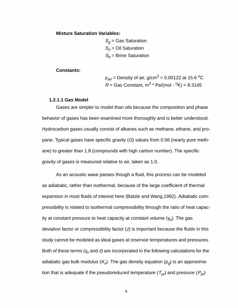
1.2.1.1 Gas Model
Gases are simpler to model than oils because the composition and phase
behavior of gases has been examined more thoroughly and is better understood.
Hydrocarbon gases usually consist of alkanes such as methane, ethane, and pro-
pane. Typical gases have specific gravity (G) values from 0.56 (nearly pure meth-
ane) to greater than 1.8 (compounds with high carbon number). The specific
gravity of gases is measured relative to air, taken as 1.0.
As an acoustic wave passes though a fluid, this process can be modeled
as adiabatic, rather than isothermal, because of the large coefficient of thermal
expansion in most fluids of interest here (Batzle and Wang,1992). Adiabatic com-
pressibility is related to isothermal compressibility through the ratio of heat capac-
ity at constant pressure to heat capacity at constant volume (γο). The gas
deviation factor or compressibility factor (z) is important because the fluids in this
study cannot be modeled as ideal gases at reservoir temperatures and pressures.
Both of these terms (γο and z) are incorporated in the following calculations for the
adiabatic gas bulk modulus (Ks). The gas density equation (ρg) is an approxima-
tion that is adequate if the pseudoreduced temperature (Tpr) and pressure (Ppr)
9

are not within about 1 of unity (Thomas et al., 1970); most gases of interest can
be modeled using the gas density equation. Using pseudoreduced values is pref-
erable because mixtures can easily be incorporated, and components such as
carbon dioxide and nitrogen can be combined by incorporating the pseudocritical
temperature (Tpc) and pressure (Ppc). The adiabatic gas modulus and the gas
density are both strongly dependent on composition. The approach used above is
commonly found and described in detail in petroleum engineering literature such
as Craft and Hawkins (1991) and McCain (1973).
Natural gases have a variable composition which complicates calculations
of the fluid properties. For pure compounds, the gas and liquid phases exist in
equilibrium along a specific pressure-temperature curve. As pressure and temper-
ature are increased, the properties of the two phases approach each other and
merge at a critical point. For mixtures, there is a range of temperature and pres-
sure for which both phases coexist, but there is still one temperature and pressure
value at which all phases are indistinguishable, called the pseudocritical tempera-
ture (Tpc) and pressure (Ppc). This pseudocritical point is a point of homogeniza-
tion and depends on the composition. The properties of mixtures are made more
systematic using as environmental conditions the pseudoreduced temperature
(Tpr) and pressure (Ppr) which are normalized by the pseudocritical temperature
and pressure.
Using the equations listed below with the input variables previously listed
allows calculation of the gas fluid properties. The terms that are not defined are
listed in Appendix A.
10

The Gas Equations:
Adiabatic Gas Modulus, Ks, in MPa:
where:
K sP
1Ppr
z---------
z∂P∂ pr
------------–
T
-----------------------------------------γo=
PprP
Ppc---------=
Ppc 4.892 0.4048G–=
z∂P∂ pr
------------ A 0.1308 3.85 T pr–( )2 DPpr1.2( )Dexp Ppr
0.2+=
A 0.03 0.00527 3.5T pr( )3+=
D 1–T pr---------
0.45 8 0.56 1T pr---------–
2+
=
T pr
T a
T pc---------=
T a T Co( ) 273.15+=
T pc 94.72 170.75G+=
γo 0.855.6
Ppr 2+( )------------------------27.1
Ppr 3.5+( )2------------------------------- 8.7 0.65 Ppr 1+( )–[ ]exp–+ +=
z 0.03 0.00527 3.5 T pr–( )3+[ ]Ppr 0.642T pr 0.007T pr4
– 0.52–( ) E+ +=
11

Gas Density, ρg, in g/cm3:
P-Wave Velocity, Vg, in m/s:
1.2.1.2 Live and Dead Oil Models
Crude oils can be mixtures of complex organic compounds and may range
from light liquids (condensates) to very heavy tars. The American Petroleum Insti-
tute (API) gravity is a widely used classification for crude oils. An API gravity of
about 5 represents a very heavy, tar-like, oil and an API gravity value near 80 rep-
resents a very light condensate. Large quantities of hydrocarbon gases can be
dissolved in oils under pressure, significantly decreasing the density and the bulk
modulus for live oils. Under surface temperature and pressure conditions the liq-
uid component (dead oil) will exhibit densities (ρo) from 0.5 g/cm3 to greater than
1 g/cm3. Variations in composition and the ability to absorb gases, produces vari-
ations in seismic properties for oil, particularly under reservoir pressures.
The density variation with pressure and temperature has been examined in
detail by McCain (1973). McCain found that the effects of pressure and tempera-
ture are largely independent from each other for oils of unchanging composition.
The pressure dependence is relatively small and can be described by the polyno-
E 0.109 3.85 T pr–( )2 0.45 8 0.56 1T pr---------–
2+
Ppr1.2
T pr----------–
exp=
ρg28.8GPzRT a
---------------------=
V g
K s
ρg-------=
12

mial given below (ρp). The effect of temperature is greater and the expression
used to calculate the density of the dead oil (ρd), live oil (ρl), and live oil saturated
with as much gas as it can possibly dissolve (ρlm, ignoring the specified gas-oil
ratio) incorporates the density at pressure, ρp (Dodson and Standing, 1945).
Wang (1988) and Wang et. al. (1988) developed a simplified velocity relationship
for ultrasonic velocities (Vd) within dead oils. This velocity depends on the temper-
ature and pressure of the reservoir and the API gravity of the oil.
The dead oil model uses the density of a dead oil at surface conditions (ρo)
to calculate the density at pressure (ρp). The live oil model uses the density at sat-
uration (ρgl) calculated from the density at surface conditions, specific gravity and
gas-oil ratio (from PVT tests), and gas volume factor (Bol) (calculated from input
values) to calculate the density at pressure, accounting for the effect of gas in
solution. The live oil model also uses a pseudodensity (ρdl) based on the expan-
sion of the oil caused by gas intake to calculate the live oil velocity (Vl, Vlm).
Using the equations below with the input variables for a specific oil and a
set of physical conditions allows calculation of the live and dead oil fluid proper-
ties. The terms that are not defined are listed in Appendix A.
The Dead Oil Equations:
Dead Oil Density, ρd, in g/cm3:
where:
ρd
ρp
0.972 3.81x 10 4–( ) T 17.78+( )1.175+[ ]-----------------------------------------------------------------------------------------------------=
ρp ρo 0.00277P 1.71x 10 7–( )P3–( ) ρo 1.15–( )2 3.49x 10 4–( )P+ +=
13

P-Wave Velocity, Vd, in m/s:
Dead Oil Modulus, Kd, in MPa:
The Live Oil Equations:
Live Oil Density, ρl, in g/cm3:
where:
P-Wave Velocity, Vl, in m/s:
ρo141.5
API 131.5+--------------------------------=
V d 15450 77.1 API+( ) 0.5– 3.7T– 4.64P 0.0115 0.36API0.5 1–( )TP+ +=
K d V d2 ρd=
ρl
ρpl
0.972 3.81x 10 4–( ) T 17.78+( )1.175+[ ]-----------------------------------------------------------------------------------------------------=
ρpl ρgl 0.00277P 1.71x 10 7– P3–+( ) ρgl 1.15–( )2 3.49x 10 4–( )P+=
ρgl
ρo 0.0012GRg+( )Bol
-------------------------------------------------=
Bol 0.972 0.0003812 2.4955RgGρo------
0.5T 17.778+ +
1.175+=
V l 2096ρdl
2.6 ρdl–----------------------
0.53.7T– 4.64P 0.0115 4.12
1.08ρdl
----------- 1– 0.5
1– TP+ +=
ρdl
ρo
Bol-------- 1 0.001Rg+( ) 1–=
14

Live Oil Modulus, Kl, in MPa:
The Equations for a Live Oil at its Maximum Gas-Oil Ratio:
Live Oil Density, ρlm, in g/cm3:
where:
P-Wave Velocity, Vlm, in m/s:
Live Oil Modulus, Klm, in MPa:
K l V l2ρl=
ρlm
ρpm
0.972 3.81x 10 4–( ) T 17.78+( )1.175+[ ]-----------------------------------------------------------------------------------------------------=
ρpm ρgm 0.00277P 1.71x 10 7– P3–+( ) ρgm 1.15–( )2 3.49x 10 4–( )P+=
ρgm
ρo 0.0012GRgmax+( )Bolm
----------------------------------------------------------=
Bolm 0.972 0.0003812 2.4955RgmaxGρo------
0.5T 17.778+ +
1.175+=
Rgmax 2.028G P 0.02877API 0.003772T–( )exp[ ]1.204=
V lm 2096ρpdm
2.6 ρpdm–---------------------------
0.53.7T– 4.64P 0.0115 4.12
1.08ρpdm------------ 1–
0.51– TP+ +=
ρpdm
ρo
Bom----------- 1 0.001Rgmax+( ) 1–=
K lm V lm2 ρlm=
15

1.2.1.3 Brine Model
The most common pore fluid is brine; its composition can range from
almost pure water to saturated saline solutions. Brine salinity is commonly one of
the easiest variables to obtain because brine resistivities are routinely calculated
during well log analysis. Simple relationships are available to convert brine resis-
tivity to salinity (e.g., Western Atlas log interpretation charts, 1996). Waters and
brines are unusual among common fluids in that their velocities begin to decrease
at very high pressures.
Increasing salinity increases the density of the brine. Using data on sodium
chloride solutions from Zarembo and Federov (1975) and Potter and Brown
(1977), Batzle and Wang (1992) constructed a simple polynomial using salinity
and reservoir temperature and pressure to calculate the density of sodium chlo-
ride solutions (ρb). This relationship is valid only for sodium chloride solutions.
Wilson (1959) provided a relationship for the velocity of water for conditions
up to 100 oC and 100 MPa. This equation is used to calculate the velocity of water
(Vw). Batzle and Wang (1992) extended the results of Millero et. al. (1977) and
Chen et. al. (1978) for brines by using a simplified form of the velocity function
provided and modifying the equation constants. The brine velocity (Vb) equation is
the modified equation (Batzle and Wang, 1992); the equation was modified to fit
additional higher temperature and higher salinity data from Wyllie et. al. (1956).
Gas can also be dissolved in a brine but the amount that can go into solu-
tion is significantly less than that of oils. The amount of gas that can go into the
brine solution increases with pressure and decreases with salinity. Rgb is the gas-
16

water ratio and defines the amount of gas that can be in solution at surface tem-
perature and pressure conditions.
Dodson and Standing (1945) found that the isothermal bulk modulus (Kgb)
for the brine solution decreases nearly linearly with gas content. This also has a
decreasing effect on the velocity.
Using the equations below with the appropriate fluid state allows calcula-
tion of the brine/water fluid properties. The terms that are not defined are listed in
Appendix A.
The Brine/Water Equations:
Density of Freshwater, ρw, in g/cm3:
Density of Brine, ρb, in g/cm3:
Velocity of Water, Vw, in m/s (constants wij are provided in Table 1-1):
Velocity of Brine, Vb, in m/s:
Modulus of Gas Free Brine, Kb, in MPa:
ρw 1 1x 10 6–( ) 80T– 3.3T 2– 0.00175T 3 489P
2TP
–
0.016T 2P 1.3x 10 5–( )T 3P– 0.333P2– 0.002T P2
–
+ +
+
(
)
(
)
+=
ρb ρw S 0.668 0.44S 1x 10 6–( ) 300P 2400PS–
T 80 3T 3300S– 13P– 47PS+ +( )+[
]+ +{
}+=
V w w ij Ti P j
j 0=
3
∑i 0=
4
∑=
V b V w S 1170 9.6T– 0.055T 2 8.5x 10 5–( )T 3– 2.6P
0.0029TP
–
0.0476P2–
+ +(
) S1.5 780 10P– 0.16P2+( ) 1820S2–
+
+
=
K b V b2ρb=
17

Modulus of Live Brine, Kgb, in MPa:
where:
1.2.1.4 Mixture Model
Properties of pore fluid mixtures containing liquid and gas phases in the
rock pores are very important from an exploration standpoint. During production,
gas may exsolve from the oil phase because of a pressure drop in the reservoir.
Due to these effects, the seismic character of the reservoir can change signifi-
cantly over time. For geophysical examinations of reservoirs, a method of deter-
mining the properties of mixed pore fluid phases is required.
Table 1-1: Coefficients for velocity of water calculation (Vw).
w00 = 1402.85 w02 = 3.437 x 10⁻³
w10 = 4.871 w12 = 1.739 x 10⁻⁴
w20 = -0.04783 w22 = -2.135 x 10⁻⁶
w30 = 1.487 x 10⁻⁴ w32 = -1.455 x 10⁻⁸
w40 = -2.197 x 10⁻⁷ w42 = 5.230 x 10⁻¹¹
w01 = 1.524 w03 = -1.197 x 10⁻⁵
w11 = -0.0111 w13 = -1.628 x 10⁻⁶
w21 = 2.747 x 10⁻⁴ w23 = 1.237 x 10⁻⁸
w31 = -6.503 x 10⁻⁷ w33 = 1.327 x 10⁻¹⁰
w41 = 7.987 x 10⁻¹⁰ w43 = -4.614 x 10⁻¹³
K gb
K b
1 0.0494Rgb+--------------------------------------=
Rgb 10log10 0.712P T 76.71– 1.5 3676P0.64+{ } 4– 7.786S T 17.78+( ) 0––
=
18

The density of a mixture (ρml, ρmlm, ρmd) is a mass balance that requires an
arithmetic volume-weighted average of the separate pore fluid phases. The effec-
tive modulus of the mixed phase fluid can be calculated easily if the pressures in
the two phases are equal. The equation used for the mixture modulus (Kol,Kolm,
Kod) is the Reuss (isostress) average of the composite solutions. If the properties
of the individual fluids and their volume fraction are known, the mixture properties
can be calculated. The mixture velocities (Vol, Volm, Vod) are then found from the
Reuss average of the fluid moduli and the mixture densities (Mavko et. al., 1998).
Using the equations below with the appropriate mixture saturation values
allows calculation of the mixture fluid properties.
The Fluid Mixture Equations:
Live Oil Mixture Density, ρml, in g/cm3:
Max Live Oil Mixture Density, ρmlm, in g/cm3:
Dead Oil Mixture Density, ρmd, in g/cm3:
Live Oil Mixture Modulus, Kol, in MPa:
Max Live Oil Mixture Modulus, Kolm, in MPa:
ρml Sgρg Soρl Sbρb+ +=
ρmlm Sgρg Soρlm Sbρb+ +=
ρmd
Sgρg Soρd Sbρb+ +=
K ol1
Sg
K s-------
So
K l-------
Sb
K g-------+ +
-----------------------------------------=
K olm1
Sg
K s-------
So
K lm----------
Sb
K g-------+ +
--------------------------------------------=
19

Dead Oil Mixture Modulus, Kod, in MPa:
Velocity for Live Oil Mixture, Vol, in m/s:
Velocity for Max Live Oil Mixture, Volm, in m/s:
Velocity for Dead Oil Mixture, Vod, in m/s:
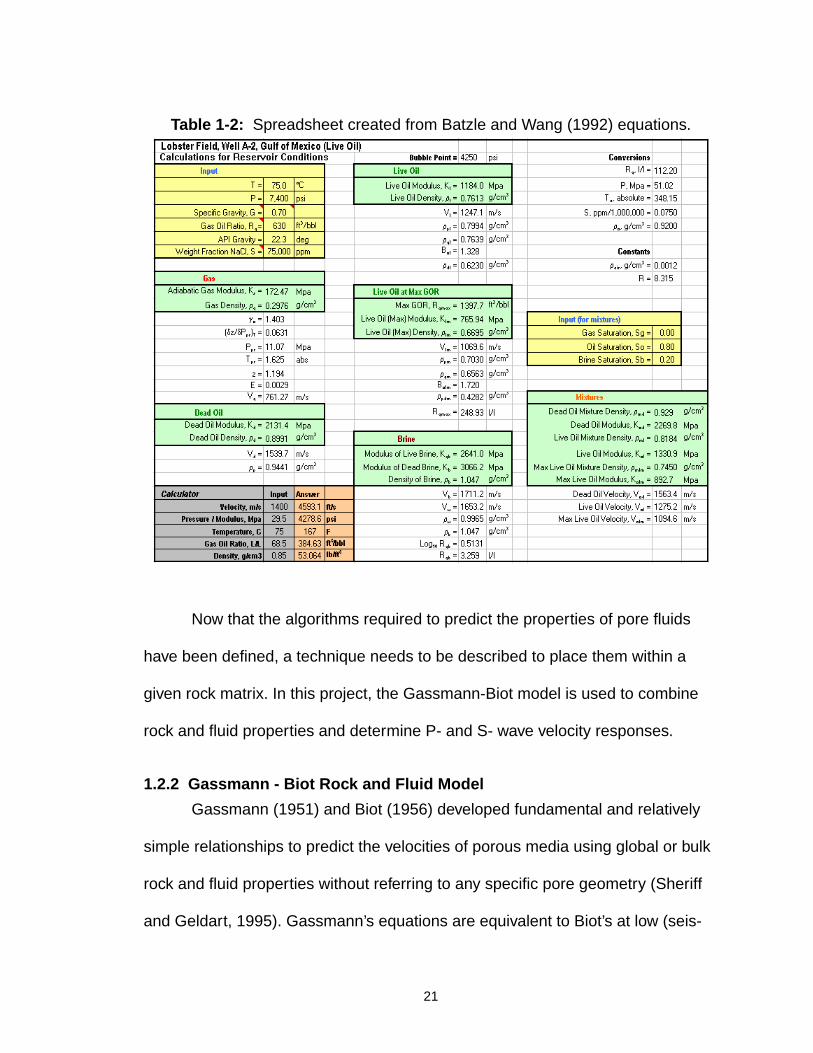
1.2.1.5 Fluid Properties Spreadsheet
Table 1-2 shows the spreadsheet created using the algorithms from the
Batzle and Wang (1992) model. The spreadsheet allows calculation of the fluid
properties for all of the models explained above, using the equations presented.
The input values, in yellow, include the reservoir temperature and pressure, gas-
oil ratio, specific gravity of the gas, API oil gravity, and salinity of the water in the
formation, as well as the relative concentrations of the fluids as a mixture. The
results, in green, consist of the velocity, density, and modulus for live oil (at speci-
fied Rg and at maximum Rg), dead oil, gas, brine, and mixtures at the conditions
entered as the input values, usually reservoir conditions.
K od1
Sg
K s-------
So
K d--------
Sb
K b-------+ +
------------------------------------------=
V ol
K ol 1000( )ρml
---------------------------=
V olm
K olm 1000( )ρmlm
-------------------------------=
V od
K od 1000( )ρmd
-----------------------------=
20
Now that the algorithms required to predict the properties of pore fluids
have been defined, a technique needs to be described to place them within a
given rock matrix. In this project, the Gassmann-Biot model is used to combine
rock and fluid properties and determine P- and S- wave velocity responses.
1.2.2 Gassmann - Biot Rock and Fluid Model
Gassmann (1951) and Biot (1956) developed fundamental and relatively
simple relationships to predict the velocities of porous media using global or bulk
rock and fluid properties without referring to any specific pore geometry (Sheriff
and Geldart, 1995). Gassmann’s equations are equivalent to Biot’s at low (seis-
Table 1-2: Spreadsheet created from Batzle and Wang (1992) equations.
21

mic) frequencies. The most significant unknown parameters are the bulk and
shear moduli of the dry rock framework (skeleton). The low-frequency Gassmann-
Biot theory predicts the resulting increase in effective bulk modulus of the satu-
rated rock when the pore pressure changes as a seismic wave passes through
the rock (Mavko et. al., 1998). These equations assume a homogeneous mineral
modulus and isotropic pore space and the effects of pressure on the dry frame
modulus are not addressed here.
There are some input variables necessary for the Gassmann-Biot model
calculations. The solid material grain bulk modulus and density are determined
from the mineralogy of the reservoir matrix. The water/brine and hydrocarbon bulk
modulus and density values are computed at reservoir temperature and pressure
conditions in the spreadsheet created for the Batzle and Wang (1992) model
described above. The P- and S- wave velocities, and bulk density (Vpi, Vsi, ρbi) val-
ues are obtained from well logs and used to calculate the saturated bulk modulus
(Kbs) and the dry frame shear modulus (G). Gassmann’s relations are used to cal-
culate the dry frame bulk modulus (Kdf) using the saturated bulk modulus (Kbs,
determined from well log or laboratory tests).
The bulk density (ρb) is calculated using a volume weighted average den-
sity for the reservoir. The fluid bulk modulus (Kf) is computed using the Reuss
(isostress) average is calculated using the water and hydrocarbon saturations.
The saturated bulk modulus (Kb) is computed at any desired saturation conditions
using the dry frame bulk modulus, solid material bulk modulus, fluid modulus, and
porosity. The compressional and shear velocities (Vp, Vs) are calculated using a
22

velocity form of Gassmann’s relation suggested by Murphy, Schwartz, and Hornby
(1991).
Input Variables:
φ = Porosity
Ks = Solid Material Bulk Modulus, GPa
ρs = Solid Material Density, g/cm3
Kw = Water Bulk Modulus, GPa
ρw = Water Density, g/cm3
Khyd = Hydrocarbon Bulk Modulus, GPa
ρhyd = Hydrocarbon Density, g/cm3
Sw = Water Saturation
Vpi = Logged P-wave velocity, m/s
Vsi = Logged S-wave velocity, m/s
ρbi = Logged Bulk Density, g/cm3
Kfi = Fluid Bulk Modulus at logged conditions, GPa
The Gassmann-Biot Equations:
Saturated Bulk Modulus, Kbs, in GPa:
Dry Frame Bulk Modulus, Kdf, in GPa:
Dry Frame Shear Modulus-Rigidity, G, in GPa:
Bulk Density, ρb, in g/cm3:
K bs ρbi V pi2 4
3---V si
2 –
10 6–=
K df K bs
φ 1–( )K s
K bs---------- φ
K s
K fi-------–+
φ 1+( )K bs
K s---------- φ
K fi
K s-------–+
----------------------------------------------------
=
G V si2 ρbi( )10 6–=
ρb 1 φ–( )ρs φSw ρw 1 Sw–( )ρhyd φ+ +=
23

Fluid Bulk Modulus, Kf, in GPa:
Saturated Bulk Modulus, Kb, in GPa:
P-Wave Velocity, Vp, in m/s:
S-Wave Velocity, Vs, in m/s:
Two other useful parameters are given below:
Poisson’s Ratio, σ:
Acoustic impedance, AI:
Using these equations with the necessary input variables allows calculation
of the overall reservoir properties taking into account the porosity, rock properties,
and fluid properties. An example of the Gassmann-Biot model applied to the Lob-
ster Field data is provided in Figure 1-5 in the results and discussions section
(section 1.3.1).
K f1
1 Sw–( )K hyd
----------------------Sw
K w--------+
-------------------------------------------=
K b
K df K s K df–( )2+
K s 1 φ–( ) K df– φK s
K f-------
+----------------------------------------------------------------=
V p
K b43---G+
ρb----------------------------
0.5
103=
V sGρb------103=
σ 0.5
V p
V s-------
22–
V p
V s-------
21–
-------------------------=
AI V pρb=
24
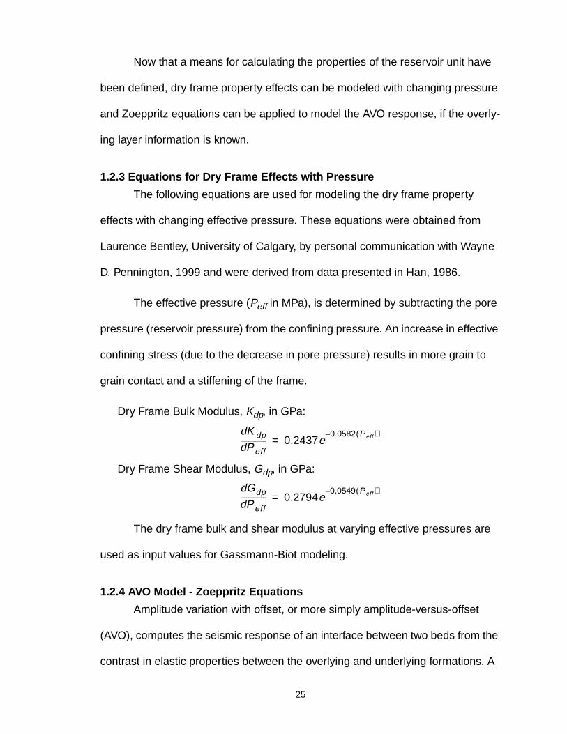
Now that a means for calculating the properties of the reservoir unit have
been defined, dry frame property effects can be modeled with changing pressure
and Zoeppritz equations can be applied to model the AVO response, if the overly-
ing layer information is known.
1.2.3 Equations for Dry Frame Effects with Pressure
The following equations are used for modeling the dry frame property
effects with changing effective pressure. These equations were obtained from
Laurence Bentley, University of Calgary, by personal communication with Wayne
D. Pennington, 1999 and were derived from data presented in Han, 1986.
The effective pressure (Peff in MPa), is determined by subtracting the pore
pressure (reservoir pressure) from the confining pressure. An increase in effective
confining stress (due to the decrease in pore pressure) results in more grain to
grain contact and a stiffening of the frame.
Dry Frame Bulk Modulus, Kdp, in GPa:
Dry Frame Shear Modulus, Gdp, in GPa:
The dry frame bulk and shear modulus at varying effective pressures are
used as input values for Gassmann-Biot modeling.
1.2.4 AVO Model - Zoeppritz Equations
Amplitude variation with offset, or more simply amplitude-versus-offset
(AVO), computes the seismic response of an interface between two beds from the
contrast in elastic properties between the overlying and underlying formations. A
K dpdPeffd
-------------- 0.2437e0.0582 Peff( )–
=
GdpdPeffd
-------------- 0.2794e0.0549 Peff( )–
=
25

normal incident, or zero offset, reflection (Ro) is readily found from the contrast in
acoustic impedance.
where:
Ro = Reflection Coefficient
ρ1 = Density of medium 1
ρ2 = Density of medium 2
V1 = Velocity in medium 1
V2 = Velocity in medium 2
The change in amplitude of the reflection coefficient with offset is a function
of the contrast in elastic properties across the interface.
AVO response is divided into three classes, Figure 1-3:
1.) A Class I AVO response has a large positive reflection at zero offset and
becomes smaller with increasing offset.
2.) A Class II AVO response has a small positive reflection at zero offset
and becomes very small or even negative with increasing offset.
Figure 1-3: Plot of reflection amplitude versus offset showing the differentclasses of AVO response.
Ro
ρ2V p2 ρ1V p1–
ρ2V p2 ρ1V p1+----------------------------------------=
R
Offset
I
II
III
26

3.) A Class III AVO response has a negative reflection at zero offset and
increasingly large negative reflections at increasing offsets. This is the classical
AVO behavior. For example, a sand-shale interface often displays a negative
reflection response that is increasingly large with offset.
Zoeppritz equations express the energy partitioning at a boundary when a
plane wave impinges on an acoustic impedance contrast (Sheriff, 1991). At a
boundary where the incident angle is zero (normal incidence) there is no mode
conversion. For example, a downward moving P-wave only generates reflected
and transmitted P-waves and a normally incident S-wave only generates reflected
and transmitted S-waves. At a boundary where the incident angle is not zero (non-
normal incidence) the seismic energy typically generates four waves, at the
boundary by splitting (mode conversion): reflected P-wave and S-wave and trans-
mitted P-wave and S-wave (Figure 1-4). Most reflections are a superposition of
events from a series of layers and will have a more complex behavior than what is
shown here.
Figure 1-4: Reflection and transmission at a boundary for an incident P-wave(from Mavko et. al., 1998).
27

Zoeppritz equations can be used to determine the amplitude of reflected
and refracted waves at this boundary for an incident P-wave. The original equa-
tions are valid for any incident waves but only the P-wave is presented here and
used in this study. The reflection and transmission coefficients depend on the
angle of incidence and the material properties of the two layers. (Mavko et. al.,
1998). The angles for incident, reflected, and transmitted rays at a boundary are
related by Snell’s law (Castagna and Backus, 1993).
Snell’s law:
where:
p = Ray parameter
Vp1 = P-wave velocity in medium 1
Vp2 = P-wave velocity in medium 2
Vs1 = S-wave velocity in medium 1
Vs2 = S-wave velocity in medium 2
Θ1 = Incident and reflected P-wave angle
Θ2 = Transmitted P-wave angle
Φ1 = Reflected S-wave angle
Φ2 = Transmitted S-wave angle
The variation of reflection and transmission coefficients with incident angle
and corresponding increasing offset is referred to as offset-dependant-reflectivity
and is the fundamental basis for AVO (Castagna and Backus, 1993).
Zoeppritz (1919) equations provide a complete solution for amplitudes of
transmitted and reflected P- and S- waves for both incident P- and S- waves. The
equations are very complex and subject to troublesome sign, convention, or typo-
graphic errors (Hales and Roberts, 1974) and Aki and Richards (1980), Shuey
pΘ1sin
V p1---------------
Θ2sin
V p2---------------
Φ1sin
V s1---------------
Φ2sin
V s2---------------= = = =
28
(1985), and Hilterman (1989) developed simplifications and approximations for
Zoeppritz equations.
Aki and Richards (1980) derived a simplified form of Zoeppritz equations
by assuming small contrasts in properties between layers, where the results are
expressed in terms of P-wave velocity, S-wave velocity, and density contrasts
across the interface.
Shuey (1985) presented another approximation to Zoeppritz equations
were the AVO gradient is expressed in terms of Poisson’s ratio (σ).
Due to the complexity of Zoeppritz equations, approximations are
extremely useful for application. The most commonly used form, due to Shuey
(1985), is given below (valid for incidence angles less than 30 degrees):
Zoeppritz Equation:
where:
R(Θ) = Reflection coefficient (function of Θ)
Θ = Angle of incidence
A = Zero-offset reflection coefficient (AVO intercept)
B = Slope of amplitude (AVO Gradient)
A is the normal incidence reflection coefficient. B describes the variation at
intermediate offsets and is called the AVO gradient or slope factor where, Ao is a
function of average values of Poisson’s ratio (σ), compressional velocity (Vp), and
R Θ( ) A B Θ( )sin2+=
A12---
∆V p
V p-----------
∆ρρ-------+
=
B AoA∆σ
1 σ–( )2--------------------+=
29
density(ρ) and the changes of Poisson’s ratio, compressional velocity and density.
A and B are both highly dependant on the properties of the reservoir and the over-
lying formation. In general, P-wave velocity is dependant on both lithology (rock
type) and fluid content. S-wave velocity is dependant on lithology, but not sensitive
to fluid content. S-wave velocities are not generally measured directly so the Vp/Vs
ratio or Poisson’s ratio is used to determine the shear velocity from the compres-
sional velocity.
This commonly used form of Zoeppritz equations has the interpretation that
the near-offset traces reveal the P-wave impedance, and the intermediate-offset
traces image contrasts in Poisson’s ratio (Castagna, 1993). Another term can be
added to account for far offsets near the critical angle, C(tan2θ - sin2θ), where
C=1/2(∆Vp/Vp) (Shuey, 1985).
Assumptions and limitations for these equations are the rock is linear, iso-
tropic, and elastic. A plane-wave propagation is assumed and most of the simpli-
fied forms assume small contrasts in material properties and no space or slipping
across the boundary (Mavko et. al., 1998).
1.3 Results and Discussion
1.3.1 Summary of Batzle and Han Data (1997 Fluid Study)
In 1997, M. Batzle and D.H. Han conducted a study of fluid properties mea-
sured on samples provided by a consortium of twenty-one supporting oil compa-
nies. The project was a joint effort led by the Houston Advanced Research Center
(D.H. Han) and the Colorado School of Mines (M. Batzle), where laboratory tests
and other work were completed.
30

The purpose of the consortium was to determine the effects of fluid density,
initial oil gravity, and gas in solution on seismic velocity of the fluid. The goals of
the Batzle and Han (1997) project were to: 1) conduct measurements of velocity
and density on 30 samples provided by industry sponsors, 2) make these data
available to consortium members in spreadsheet format, 3) develop empirical
relations to describe oil properties, 4) link static pressure-volume-temperature
(PVT) data to seismic properties, and 5) develop a program to calculate fluid prop-
erties under realistic conditions. This summary will focus on the velocity and den-
sity measurements from the study and how they compare to values computed
from the Batzle and Wang (1992) model. Some samples were not analyzed at the
presumed reservoir temperature and pressure conditions of 80-90 oC and 6000
psi that were used for calculations in this thesis study, and are not included in the
plots or calculations. This laboratory data is used to determine the usefulness of
the Batzle and Wang (1992) model as a predictive tool.
The samples used in the laboratory tests included live oils that were recon-
stituted from dead oils. In general, the live oil was reconstituted based on the com-
position report from the PVT data. The samples were subjected to temperature
and pressure conditions above the bubble point and different gases were added
based on weight percent until the GOR reached the value reported for the reser-
voir and the fluid was in a single oil phase.
Figure 1-5 shows the locations of most of the oil samples studied in the
Batzle and Han (1997) fluids consortium. The samples are from the United States
(AK, WY, NM, TX), the Gulf of Mexico, the North Sea, and Indonesia. This
31

distribution provides a variety of depositional environments and reservoirs and
gives a good overall sample set to study.
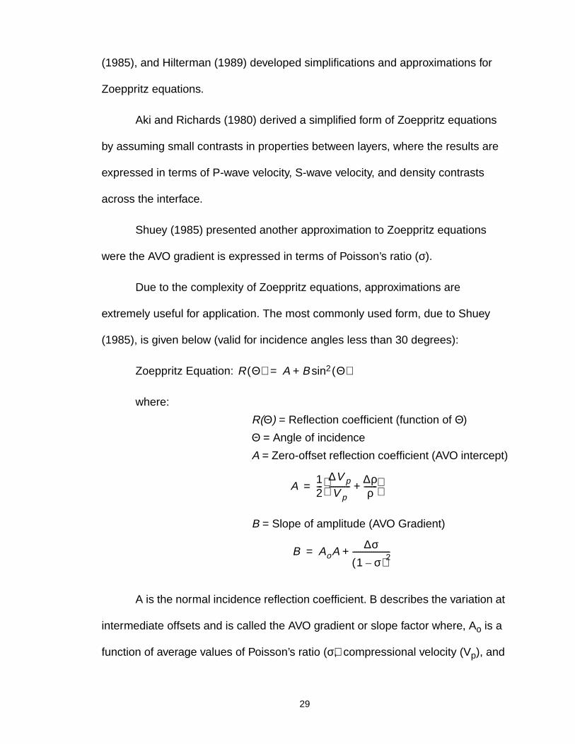
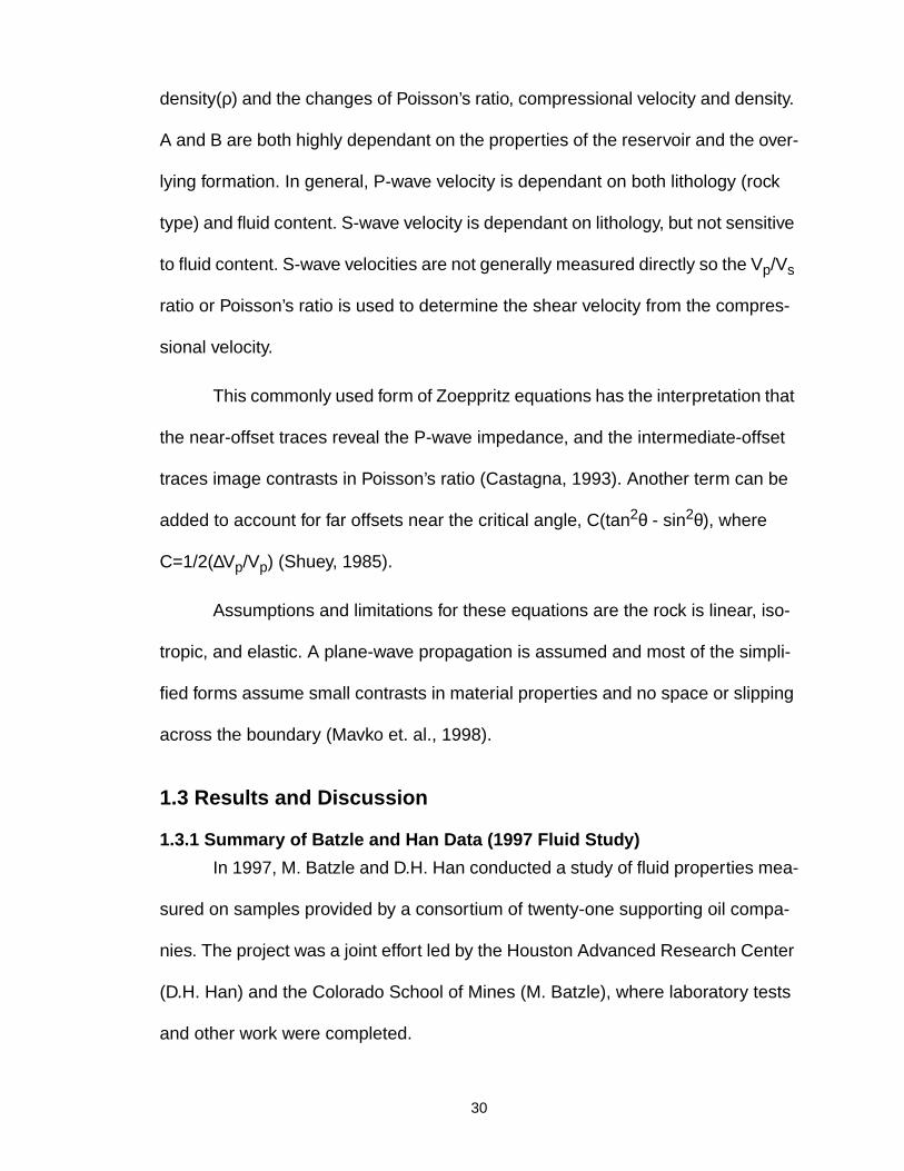
The distributions of API gravity and GOR values for the samples in the
study are included in Figure 1-6 and Figure 1-7, respectively. The oils in the study
consist of mostly middle range API gravity values. Very few light or heavy oils
were included in this study. The distribution of GOR is broad but oils with an
extremely high GOR are missing. The API and GOR are indicated for an oil from
the Lobster Field (Gulf of Mexico) for reference. The sample for the Lobster Field
is analyzed in detail later in this thesis.
Figure 1-5: Location of fluid samples studied in the Batzle and Han (1997) fluidsproject consortium.
32
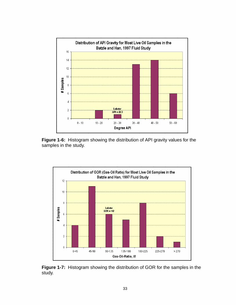
Figure 1-6: Histogram showing the distribution of API gravity values for thesamples in the study.
Figure 1-7: Histogram showing the distribution of GOR for the samples in thestudy.
33

Figures 1-8 through 1-13 compare the summary data from the Batzle and
Han (1997) fluids project and calculations based on the Batzle and Wang (1992)
model. The calculated values were computed using the spreadsheet presented in
section 1.2.1, using the Batzle and Wang (1992) model, and are based on input
values from reservoir conditions (given in the Batzle and Han (1997) fluid study).
The measured values selected for plotting are those conducted under conditions
most similar to reservoir conditions (approximately 80-90 oC and 6000 psi). Some
samples were not analyzed at these reservoir conditions used for calculations and
are not included in the study.
Figure 1-8: Plot showing the calculated live oil velocity (Batzle and Wang 1992Model) versus the laboratory live oil velocity (Batzle and Han 1997 Fluid Study).
Perfect Correlation
34

Figure 1-8 shows the live oil laboratory velocities tested in the Batzle and
Han (1997) fluid study plotted versus the calculated live oil velocities from the Bat-
zle and Wang (1992) model. The diagonal dashed line represents a perfect corre-
lation. This figure shows that the Batzle and Wang (1992) model is in general
quite good for predicting the velocity observed in the laboratory, although it slightly
but consistently underestimates the live oil velocity compared to the measured
laboratory live oil velocities. In order to investigate the dependence of live fluid
velocity on the various input parameters, the calculated velocity, density, and mod-
ulus is plotted versus various parameters for the specific oils used in the Batzle
and Han (1997) fluid study.
Figure 1-9 shows the live and dead oil density and how these properties
correlate with the gas-oil ratio. The computed dead oil density is plotted versus the
gas-oil ratio for the original oil in-situ (live oil). The dead oil density is calculated at
surface conditions and the live oil is calculated at reservoir conditions, from the
same API gravity and GOR which were reported for the individual samples. The
trend of data for live oil density demonstrates that as the gas-oil ratio increases,
the density of the oil decreases. It is interesting to note that there is no obvious
correlation between the dead oil density (or API gravity) and the gas in solution as
found under reservoir conditions.
Figure 1-10 shows that the solution gas-oil ratio has a large effect on the
velocity for the samples in the study. As the gas-oil ratio increases, the velocity of
the live oil decreases significantly. This demonstrates that even a small amount of
gas in solution has a large effect on the fluid compressibility. The gas in solution
35
also decreases the density of the live oil (see Figure 1-9), but not enough to over-
come the effect of increased compressibility on the velocity.
Figure 1-11 is a plot of calculated velocity versus API gravity for the live oil
samples involved in the study. In general, as the API gravity increases, the velocity
of the live oil decreases, but the effect is much smaller than for the solution gas-oil
ratio.
Figure 1-12 is a cross plot of the calculated live oil modulus versus calcu-
lated live oil density for the samples in the study. Note that the data set has an
exponential trend. This is apparently due to the high compressibility and low
Figure 1-9: Plot of live and dead oil densities for the samples in the study and therelationship to GOR (the lines are a least squares regression through the datapoints).
36

Figure 1-10: Plot of the calculated velocity versus GOR for the samples in thestudy.
Figure 1-11: Plot of the calculated velocity versus API gravity for the samples inthe study.
37

density of the lighter hydrocarbons that are in the gas phase at surface conditions
yet are in solution under reservoir conditions. The live oil modulus decreases as
the live oil density decreases due to the increasing compressibility in the system.
Figure 1-13 is a plot of the calculated live oil velocity versus the calculated
live oil density for the samples in the study, showing a strong correlation, where
the velocity of the oil decreases as the density decreases. The modulus
decreases so rapidly with density that the overall effect on velocity is a decrease
in velocity with density.
Figure 1-12: Plot of calculated live oil modulus versus density for the samples inthe study.
38

Figure 1-14 is a plot of the laboratory velocity and calculated velocity data
versus pressure for a specific sample (Marathon Oil Company, Well A-2) in the
Batzle and Han (1997) fluid study. The calculated velocity data was modeled
assuming a constant GOR of 112.2 l/l (630 ft3/bbl). The data shows that the Batzle
and Wang (1992) model, indicated by the solid symbols connected by lines,
underestimates the laboratory data shown by the open unconnected symbols.
The bubble point for this sample is at 29.3 MPa (4250 psi) at 75 oC (reservoir tem-
perature). Notice that at pressure below the bubble point the laboratory data and
predicted data diverge significantly. This is due to the fact that the laboratory mea-
surements were made on only the oil fraction as the gas exsolved from solution
Figure 1-13: Plot of live oil velocity versus density for the samples in the study.
39

and the GOR in that oil fraction changes below the bubble point. However, the
GOR of the oil fraction is held constant in the calculations. Figure 1-14 also shows
that temperature affects the disagreement between the calculated and measured
values above the bubble point pressure, with the disagreement becoming greater
at lower temperature, and is very small at reservoir conditions.
Figure 1-15 helps to explain the discrepancy between the calculated values
(assuming constant GOR) and the laboratory values below the bubble point pres-
sure. The term "black oil" refers to reservoirs containing immiscible water, oil and
gas phases with a simple pressure-dependant solubility of the gas component in
the oil phase. The composition of the oil and gas components are assumed to be
Figure 1-14: Plot showing the calculated live oil velocity (Batzle and Wang 1992Model) and the laboratory live oil velocity (Batzle and Han 1997 Fluid Study)versus pressure for a sample in the study modeled with constant GOR.
40

constant at all pressure conditions (Bradley, 1987). In such a model, it is assumed
that at reservoir pressure conditions, the live oil has a specified GOR (normally
determined from PVT testing), and as pressure decreases, but remains above the
bubble point, the GOR of the live oil remains constant. When the pressure
reaches the bubble point, free gas begins to come out of solution and the GOR of
the liquid oil decreases. As the pressure drops further, more free gas comes out of
solution and the GOR of the liquid oil continues to decrease. The GOR of the liq-
uid oil below the bubble point is referred to as the maximum GOR at specified
temperature and pressure conditions.
Figure 1-16 is another plot of the laboratory velocity and calculated velocity
data versus pressure for a specific sample (Marathon Oil Company, Well A-2) in
Figure 1-15: The evolution of hydrocarbon phases with decreasing pressure. Theliquid component (oil) is best described as the "live" oil calculated at the specifiedGOR above the bubble point pressure, and by the maximum GOR at conditionsbelow the bubble point pressure.
41

the Batzle and Han (1997) fluid study. In this case, the calculated velocity data
was modeled with a constant GOR of 112.2 l/l (630 ft3/bbl) above the bubble point
pressure and a variable GOR (the maximum GOR at the specified pressure and
temperature conditions) below the bubble point. The data shows that the Batzle
and Wang (1992) model still underestimates the laboratory data, similar to Figure
1-14, but fits much more closely below the bubble point where the GOR of the oil
fraction varies. Figure 1-16 also shows that the difference between the laboratory
and calculated values decrease with increasing temperature at high pressures but
at pressures near the bubble point the difference increases with increasing tem-
perature. The error between the modeled data and the laboratory data increases
Figure 1-16: Plot showing the calculated live oil velocity (Batzle and Wang 1992Model) and the laboratory live oil velocity (Batzle and Han 1997 Fluid Study)versus pressure for a sample in the study modeled with a variable GOR.
42

near the bubble point because constant composition of the oil and gas is assumed
yet compositional variations are, most likely, an important factor near the bubble
point.
The following section will focus on more in-depth modeling of Well A-2
using the Batzle and Wang model, the Gassmann-Biot model, and the AVO model
described above in sections 1.2.1, 1.2.2, and 1.2.3, respectively. Because the Bat-
zle and Wang model adequately describes the oil velocities under reservoir condi-
tions, it is assumed that it can be used to model conditions of reservoir depletion
during production.
1.3.2 Application to Lobster Field, Well A-2
The Lobster Field, located in Ewing Bank block 873 in the Gulf of Mexico,
was discovered in late 1991. The field is located approximately 200 miles south of
New Orleans, Louisiana and the platform (shown in Figure 1-17) is in approxi-
mately 775 feet of water. The field produces from an overpressured reservoir, in a
formation marked by the Bulminella foraminifera (Bul-1 formation), of Pliocene
age, at a depth of about 11,000 ft subsea (Petro et. al., 1997). The Bul-1 formation
consists of poorly consolidated turbidite sands with a porosity of approximately 30
percent. The trapping mechanism is a combination stratigraphic and structural
trap, shown in Figure 1-18. It lies along the flexure trend between the current shelf
and continental slope and at the north end of a semi-circular salt withdrawal basin.
Hydrocarbon migration is believed to have occurred along faults from a deep,
Jurassic age, high sulfur, carbonate source (Petro et. al., 1997).
43
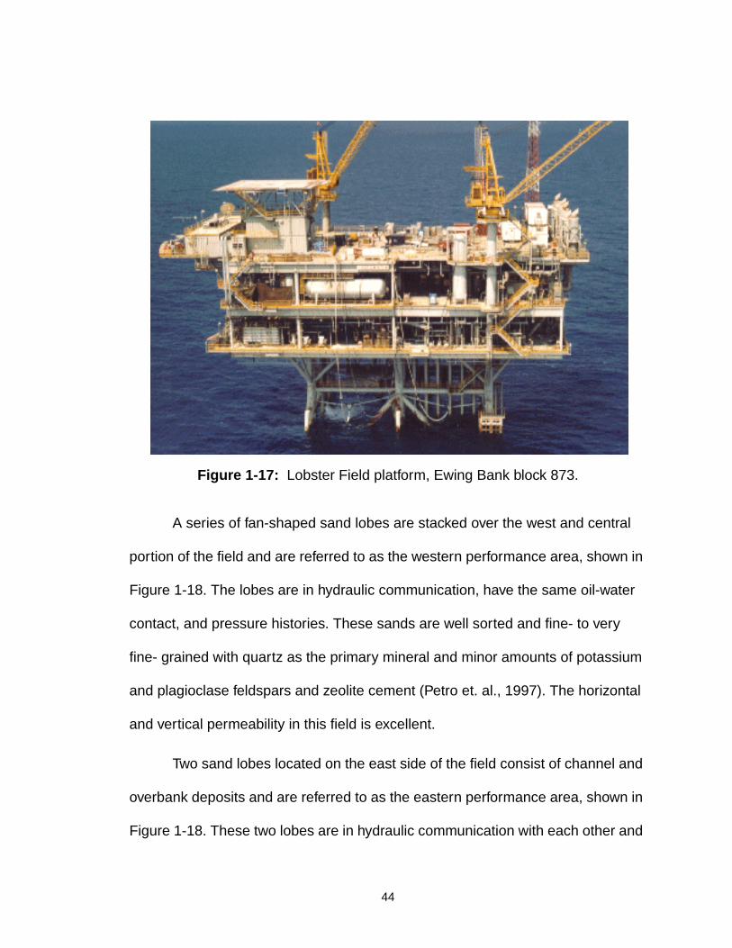
A series of fan-shaped sand lobes are stacked over the west and central
portion of the field and are referred to as the western performance area, shown in
Figure 1-18. The lobes are in hydraulic communication, have the same oil-water
contact, and pressure histories. These sands are well sorted and fine- to very
fine- grained with quartz as the primary mineral and minor amounts of potassium
and plagioclase feldspars and zeolite cement (Petro et. al., 1997). The horizontal
and vertical permeability in this field is excellent.
Two sand lobes located on the east side of the field consist of channel and
overbank deposits and are referred to as the eastern performance area, shown in
Figure 1-18. These two lobes are in hydraulic communication with each other and
Figure 1-17: Lobster Field platform, Ewing Bank block 873.
44

are separated from the western performance area. The sands are fine- to very
fine- grained with smectite, volcanic fragments, and zeolite cement present with
quartz, the predominant mineral. Lamination is more prevalent here than the
western performance area (Petro et. al., 1997).
This study will focus on the eastern performance area, specifically Well A-2
(completed in October, 1994), located on Figure 1-18, which contains an under-
saturated oil system at a reservoir temperature of 75 oC (167 oF) and pressure of
7400 psi (51 MPa). The height of the oil column is approximately 4350 feet and
Well A-2 has a completion interval of 121 feet (Petro et. al., 1997).
Figure 1-18: Structure and performance areas (from Petro et.al., 1997).
Well used in study
45

Figure 1-19 is a flow chart showing the approach used in this thesis to
model the reservoir with changing saturation and pressure conditions. First, the
reservoir is modeled with varying saturation and constant pressure conditions
using the Batzle and Wang and Gassmann-Biot models. The results from this
approach are shown in Figures 1-20 and 1-22 through 1-25. The reservoir is then
modeled varying both saturation and pressure conditions using the Batzle and
Wang, Gassmann-Biot, and AVO (seismic) models. The dry frame changes with
pressure are also modeled using an equation obtained from Laurence Bentley
(University of Calgary, personal communication, July 1999). The results from this
approach are shown in Figures 1-26 through 1-30 (section 1.3.2.1).
Essential input parameters for the Batzle and Wang (1992) model were
obtained from PVT testing on an oil sample from Well A-2 (taken at approximately
Figure 1-19: Flow chart showing the approach to reservoir modeling withchanging saturation and pressure conditions.
46

12,000 feet depth). The gas specific gravity (G) is 0.70, the gas-oil ratio is 121
liter/liter (630 ft3/bbl), the API gravity is 22.3, and the salinity of the brine in the for-
mation is 75,000 ppm. These values are input to the spreadsheet created from the
Batzle and Wang (1992) model, shown in Table 1-3. The values are then com-
puted for velocity, density, and modulus for a gas, live oil, dead oil, and brine using
the equations that are described above in the Batzle and Wang model. It is evi-
dent in Table 1-3 that the amount of gas in solution has a significant effect on the
fluid properties.
The densities for a live and dead oil are 0.7613 and 0.8991 g/cm3, respec-
tively, at reservoir conditions. The moduli for a live and dead oil are 1184.0 and
Table 1-3: Spreadsheet based on Batzle and Wang (1992) predictors showingthe calculation of fluid properties for Well A-2, Lobster Field.
47

2131.4 MPa, respectively, at reservoir conditions. These model results yield veloc-
ities for live and dead oil of 1247.1 and 1539.7 m/s, respectively, at reservoir con-
ditions. Calculations have also been made for certain fluid mixtures, which provide
more realistic views of this reservoir. The spreadsheet shown in Table 1-3 gives
the results for a mixture of 80 percent oil and 20 percent brine (a good estimate for
irreducible water saturation in the unproduced and uninvaded reservoir); addi-
tional calculations were made for other mixtures.
Table 1-4 gives the values for different mixtures of the Lobster fluids (used
to create the modulus density crossplot in Figure 1-20), computed using the mix-
tures feature in the spreadsheet of Table 1-3. These data demonstrate how the
fluid properties in the reservoir will change through time as fluid saturation
changes during production. Water begins to move through the reservoir due to
water injection and oil production, and gas comes out of solution due to a
decrease in pressure below the bubble point. The reservoir was discovered at irre-
ducible water saturation, eighty percent live oil and twenty percent water; this
point is the second green square above the live oil box in Figure 1-20. As more
water is introduced into the system as the reservoir is produced, the reservoir
properties will move upward along the green line (X-A), assuming as this time that
the pressure does not change.
The moduli are calculated as functions of changing saturation, but the
pressure and temperature conditions are not assumed to change in the construc-
tion of Figure 1-20. This is a significant simplification, but calculations based on
reasonable pressure drops with production (up to 2500 psia) show that the satura-
48

tion change itself is much more significant than the pressure change as it affects
each phase separately. The pressure change, of course, is accompanied by a sat-
uration change. If the pressure and saturation changes are modeled simulta-
neously, the modulus decreases rapidly (as gas is liberated) and the density
decreases slowly.
This decrease in pressure (modeled here as changing saturation with pres-
sure constant) with production has little effect on the fluid properties until the bub-
ble point is reached. Once the bubble point is reached the reservoir changes from
a two phase (oil-water) system to a more complex three phase (oil-gas-water) sys-
tem, as gas begins to exsolve from the live oil. This transformation is significant
Table 1-4: Modulus and density values for Lobster Field as fluid saturationchanges during reservoir production.
49

because even a small amount of gas has a very large effect on the fluid proper-
ties. The oil-gas-water saturations are posted along the orange line and the gas-
water properties are posted along the red line in Figure 1-20. The large effects
due to gas are obvious. There are significant decreases in the modulus and den-
sity values with a small amount of gas in the system, as little as 5 percent.
Figure 1-20: Crossplot of fluid modulus and density as saturation values change.The saturation change, in percent, are given for (oil, gas, water) in the labels.
X
A
50

A likely path for the fluid properties of the reservoir during production is
shown as a solid black line in Figure 1-20. This shows the effect of, first, water
encroachment (trajectory X-A), and later, the evolution of a gas phase as the pres-
sure drops below bubble point. The effect of changing saturation can be incorpo-
rated into a model for the host rock (Gassmann-Biot model), in order to investigate
its effect on bulk seismic properties of the formation, and later, into a layered earth
model to predict the seismic response as the reservoir is depleted. This will aid in
production and reservoir engineering decisions and forecasting.
Figure 1-21 is a well log for Well A-2, Lobster Field, showing gamma ray,
resistivity, P-wave velocity, and bulk density. The yellow blocks on the gamma ray
curve, in green, are sands and the orange blocks are shales. The resistivity curve,
in orange, shows high resistivity kicks (oil zones) which are shaded in green. The
oil zone at approximately 12,000 feet is the reservoir unit in the Bul 1 formation.
Notice that the P-wave velocity, in red, and the density, in black, both decrease in
the oil zone. In contrast, a water-saturated sand is located at approximately
11,800 feet and does not show a decrease in P-wave velocity. The bulk density
decreases slightly in the sands due to the change in lithology.
The layer above the reservoir unit is shale and has a value of 2900 m/s
(9500 ft/s) for P-wave velocity, 1250 m/s (4100 ft/s) S-wave velocity (not shown on
the log) and 2.4 g/cm3 for bulk density. The reservoir unit is a sand (Bul-1 forma-
tion) and has an average value of 2225 m/s (7300 ft/s) for P-wave velocity, 1280
m/s (4200 ft/s) for S-wave velocity (not shown on the log), and 2.1 g/cm3 for bulk
51

density. These properties for the reservoir unit and overlying layer are needed to
determine the AVO response of the boundary between the two layers.
Table 1-5 demonstrates the use of the Gassmann-Biot equations with fluid
and rock properties to determine the overall reservoir rock seismic properties
such as velocity and density. The input values include porosity, solid material bulk
modulus (Ks) and density (ρs), brine density and bulk modulus (ρw, Kw), and
hydrocarbon density and bulk modulus (ρhyd, Khyd). The important output values
Figure 1-21: Well log showing gamma ray, resistivity, compressional (P-wave)velocity, and bulk density curves for Well A-2, Lobster Field.
ft/s g/cm3
52

are the bulk density (ρd), P-wave velocity (Vp), S-wave velocity (Vs), acoustic
impedance (AI), and Poisson’s ratio (σ) as they vary due to changes in saturation.
The dry frame modulus is held constant.
Figure 1-22A shows P- and S- wave velocity and bulk density as a function
of water saturation, the result of fluid substitution into the Gassmann-Biot equa-
tions. The shear wave velocity (Vs, green curve) is not significantly affected by the
change in saturation, because it is not affected by the change in fluid saturation
but it is affected by the slight change in density. The compressional wave velocity
(Vp, red curve) trends from 2605 m/s (8545 ft/s) at full water saturation to 2229 m/
s (7312 ft/s) at full oil saturation. At reservoir conditions, the saturation during
Table 1-5: Gassmann-Biot model to calculate velocity and densityat various water saturation conditions (core samples measured at0.26, 0.39. and 0.53 saturation).
53
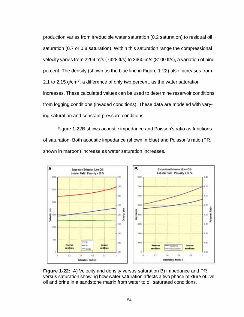
production varies from irreducible water saturation (0.2 saturation) to residual oil
saturation (0.7 or 0.8 saturation). Within this saturation range the compressional
velocity varies from 2264 m/s (7428 ft/s) to 2460 m/s (8100 ft/s), a variation of nine
percent. The density (shown as the blue line in Figure 1-22) also increases from
2.1 to 2.15 g/cm3, a difference of only two percent, as the water saturation
increases. These calculated values can be used to determine reservoir conditions
from logging conditions (invaded conditions). These data are modeled with vary-
ing saturation and constant pressure conditions.
Figure 1-22B shows acoustic impedance and Poisson’s ratio as functions
of saturation. Both acoustic impedance (shown in blue) and Poisson’s ratio (PR,
shown in maroon) increase as water saturation increases.
Figure 1-22: A) Velocity and density versus saturation B) impedance and PRversus saturation showing how water saturation affects a two phase mixture of liveoil and brine in a sandstone matrix from water to oil saturated conditions.
A B
54

The properties of the pore fluids have significant effects on the impedance
and Poisson’s ratio of the reservoir rock as shown in Figure 1-23A. This figure
shows changes in the impedance and Poisson’s ratio values as the reservoir
(shown as point X in Figure 1-20) becomes more water-saturated. The impedance
and Poisson’s ratio can be directly correlated to the seismic amplitude and ampli-
tude variation with offset at the interface between the overlying shale and the res-
ervoir. At reservoir conditions, the impedance is 4755 m/s*g/cm3 (15,600 ft/s*g/
cm3) and Poisson’s ratio is 0.27. The impedance and Poisson’s ratio of the reser-
voir formation increase as the water saturation increases and the reservoir
becomes depleted. At full water saturation, the impedance is 5650 m/s*g/cm3
(18,536 ft/s*g/cm3) and Poisson’s ratio is 0.35.
The smaller impedance value at reservoir conditions produces a larger
impedance contrast with the overlying shale layer which in turn creates a larger
amplitude seismic response. The smaller Poisson’s ratio at reservoir conditions
produces a large contrast between the reservoir formation and the overlying shale
layer, in turn creating a class III amplitude variation with offset (AVO) effect.
Figure 1-23B shows the predicted percent changes in impedance and
Poisson’s ratio of the reservoir rock due to changes in the pore fluid properties.
The point labeled reservoir conditions in Figure 1-23A and B is related to point
labeled X in Figure 1-20. If the water saturation increases, the fluid bulk modulus
and density increase according to the trajectory labeled X-A in Figure 1-20, this
has an increasing affect on Poisson’s ratio and the acoustic impedance. There is a
12 percent increase in impedance and a 21 percent increase in Poisson’s ratio as
55

saturation values change from reservoir conditions (0.2 water saturation) to resid-
ual oil conditions (0.7 water saturation), when the reservoir is depleted.
Figure 1-24 is a plot of the compressional velocity of a compressional wave
passing through the fluid and rock matrix versus the bulk density. This figure
shows the changes in velocity and density values as the reservoir becomes
increasingly water saturated. At reservoir conditions, the velocity is 2264 m/s
(7428 ft/s) and the density is 2.10 g/cm3. The velocity and density of the reservoir
increase as the water saturation increases and the reservoir becomes depleted.
At full water saturation, the velocity is 2605 m/s (8545 ft/s) and the density is 2.17
g/cm3.
Figure 1-23: A) Impedance versus PR B) Percent change in impedance versuspercent change in PR showing how water saturation affects a two phase mixtureof live oil and brine in a sandstone matrix from water saturated to oil saturatedconditions.
A
wet
depleted
conditionsreservoir
wet
depleted
conditionsreservoir
A B
wet
depleted
conditionsreservoir
56

Figure 1-25 is a graph of shear velocity versus compressional velocity. The
shear velocity changes very little as water saturation increases while the compres-
sional velocity changes significantly. The compressional velocity is much more
susceptible to fluid changes and is used to help determine fluid properties. The
shear velocity is useful in determining frame properties and is not affected by flu-
ids in the reservoir.
Figure 1-24: P-wave velocity versus density showing how water saturationaffects a two phase mixture of live oil and brine in a sandstone matrix from watersaturated to oil saturated conditions.
wet
depleted
reservoirconditions
57

1.3.2.1 Predicted Reservoir Response to Production for Lobster Field
In this section, the previously developed models will be used to evaluate
the dependence of seismic properties on saturation and pressure changes
expected during reservoir production. The following figures illustrate how the pre-
dictors may be used to model the reservoir through time as it is produced and the
pressure decreases. Figures 1-26 and 1-27 are concerned with fluid properties
above while Figures 1-28A and 1-29 show the effect of changing both saturation
and pressure conditions within a rock assuming a constant dry frame modulus.
Figures 1-28B and 1-30 show the effect of varying saturation and pressure condi-
tions while also assuming the dry frame modulus is a function of pressure.
Figure 1-25: Compressional vs. shear velocity for a two phase mixture of live oiland brine in a sandstone matrix from water saturated to oil saturated conditions.
wetdepleted
reservoirconditions
58
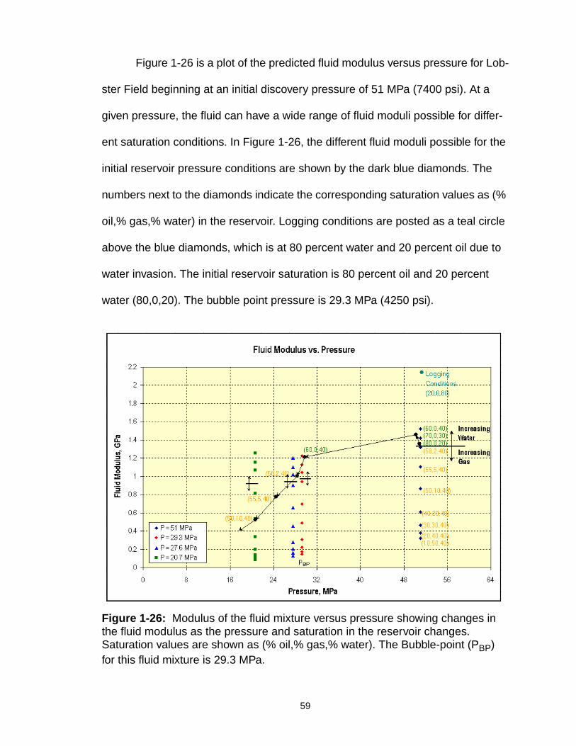
Figure 1-26 is a plot of the predicted fluid modulus versus pressure for Lob-
ster Field beginning at an initial discovery pressure of 51 MPa (7400 psi). At a
given pressure, the fluid can have a wide range of fluid moduli possible for differ-
ent saturation conditions. In Figure 1-26, the different fluid moduli possible for the
initial reservoir pressure conditions are shown by the dark blue diamonds. The
numbers next to the diamonds indicate the corresponding saturation values as (%
oil,% gas,% water) in the reservoir. Logging conditions are posted as a teal circle
above the blue diamonds, which is at 80 percent water and 20 percent oil due to
water invasion. The initial reservoir saturation is 80 percent oil and 20 percent
water (80,0,20). The bubble point pressure is 29.3 MPa (4250 psi).
Figure 1-26: Modulus of the fluid mixture versus pressure showing changes inthe fluid modulus as the pressure and saturation in the reservoir changes.Saturation values are shown as (% oil,% gas,% water). The Bubble-point (PBP)for this fluid mixture is 29.3 MPa.
59

The black line connecting several data tracks is the expected modulus
response to pressure changes. The line starts at the initial reservoir saturation
point (80,0,20) and slightly increases as water begins to invade the reservoir. The
effects of pressure then take over and the modulus begins to drop slightly as it
approaches the bubble point. Once the bubble point is reached, the modulus of
the reservoir drops significantly as free gas begins to exsolve in the system. The
modulus continues to decrease significantly as the pressure drops further and
more gas exsolves from solution. The saturation of the fluids and gas in the reser-
voir is posted at several points along the black line.
Figure 1-27 shows the fluid density of the reservoir versus pressure. The
black line on the plot is the expected density response to pressure and saturation
changes in the reservoir. The saturation of the fluids and gas in the reservoir is
posted at several points along the black line in the same format as Figure 1-26.
The density is not affected as strongly as the modulus by pressure changes and
variations of saturation. The expected conditions start at the initial reservoir satu-
ration point (80,0,20) and slightly increase as water begins to invade the reservoir.
Once the bubble point is reached and gas begins to exsolve into the reservoir the
density begins to decrease more drastically.
This change in modulus and density will affect the reservoir properties over
time. As the pressure drops, the fluid modulus and density also drop significantly
when free gas is introduced into the reservoir. The changes in density and modu-
lus will also change the P-wave velocity and Poisson’s ratio in the reservoir unit.
60

Figure 1-28A shows the decrease in both P-wave velocity and Poisson’s
ratio as the pressure in the reservoir decreases below the bubble point and satu-
ration changes. The dry frame modulus is held constant.
The equations for the dry frame bulk and shear moduli with changing effec-
tive pressure (Peff in MPa) are listed below and are calibrated for the Lobster Field
using known values at reservoir conditions.
Dry Frame Bulk Modulus, Kdp, in GPa:
Dry Frame Shear Modulus, Gdp, in GPa:
Figure 1-27: Fluid density versus pressure showing how the density changesas the pressure and saturation in the reservoir changes.Saturation values areshown as (% oil,% gas,% water).
K dp 4.1873e0.0582 Peff( )–
– 3.61+=
Gdp 5.089e0.0549 Peff( )–
– 4.714+=
61

Figure 1-28B also shows the decrease in both P-wave velocity and Pois-
son’s ratio as the pressure in the reservoir decreases below the bubble point and
saturation changes where the dry frame modulus changes with pressure. Notice
that a variable dry frame modulus decreases the Poisson’s ratio and increases the
P-wave velocity. The effects of the dry frame are due to the stiffening of the frame
as pressure decreases. The dry frame effects counteract the effects of free gas in
the reservoir. The changes in these variables will affect the seismic signature of
the reservoir over time (as pressure decreases). The decrease in P-wave velocity
and Poisson’s ratio will increase the impedance contrast with the overlying shale
layer and amplify the AVO effect.
Figure 1-29 shows the AVO response for the reservoir as pressure and
fluid saturations change. The dry frame effects are held constant. The green
Figure 1-28: Velocity and Poisson’s ratio versus pressure demonstrating thatwhen the reservoir drops below the bubble point (at 29.3 MPa) it significantlyeffects the reservoir properties. A) Modeled with a constant dry frame modulus.B) Modeled with a variable dry frame modulus with pressure.
A B
reservoirbubble conditionspoint
reservoirbubble
conditionspoint
62

series are those that are saturated with oil and water (containing no free gas). The
red series are saturated with oil, free gas, and water (saturation values are listed
in the legend as %oil,%gas,%water). The series are labeled P1 through P6. P1
corresponds to initial reservoir conditions when the field was discovered; P2-P6
show the progression through time as the pressure drops and gas begins to
exsolve from solution at the same pressure as previous plots. It is apparent that
the AVO response becomes more pronounced as free gas exsolves from the live
oil when the pressure drops below the bubble point (P4, P5, P6), assuming dry
frame effects with pressure are held constant. Although not shown, the response
calculated from logging conditions is nearly identical to the AVO response at 60
percent oil and 40 percent water saturation (4250 psi), shown as P3.
Figure 1-29: Reflection amplitude versus offset showing the amplitude variationwith offset as the pressure changes over time. Saturation values are shown inlegend as (% oil,% gas,% water).
Time
63

Figure 1-30 shows the AVO response for the reservoir as the dry frame and
fluid saturation changes with pressure. The green series are those that are satu-
rated with oil and water (containing no free gas). The red series are saturated with
oil, free gas, and water (saturation values are listed in the legend). The dry frame
changes with pressure are included. The series are labeled P1 through P6. P1
corresponds to initial reservoir conditions when the field was discovered; P2-P6
show the progression through time as the pressure drops and gas begins to
exsolve from solution. The AVO response decreases as water saturation
increases (P1 to P3) then as free gas exsolves from the live oil, when the pressure
drops below the bubble point (P4 to P6), the AVO response increases.
Figure 1-30: Reflection amplitude versus offset showing the amplitude variationwith offset as the pressure changes over time including the effects on the dryframe. Saturation values are shown in legend as (% oil,% gas,% water).
Time
64

This result is very important because the AVO response at P5, a pressure signifi-
cantly below the bubble point, is the same as the AVO response at initial reservoir
conditions, P1.
1.4 ConclusionsThe Batzle and Wang (1992) model predicts the Batzle and Han (1997)
data reasonably well. The model slightly underpredicts the velocity of live oils and
overpredicts the velocity of dead oils. The model error increases as temperature
increases and does not match live oil laboratory data below the bubble point due
to experimental conditions. As a result, this model can be used for specific reser-
voir cases.
Gas-oil ratio affects fluid properties by decreasing density, modulus, and
velocity with increasing GOR. The compressibility of the fluid increases as the gas
in solution increases. As temperature increases the velocity and density of the
fluid decreases. The decrease in velocity as API gravity increases may be due to
the composition of the sample and an increase in compressibility.
The density and modulus can be calculated at different saturation and
pressure conditions using the Batzle and Wang model and then plotted on a
crossplot. This allows prediction of fluid properties as the reservoir is produced
and shows the effect on the reservoir as it drops below bubble point.
Using the Batzle and Wang and Gassmann-Biot model, the change in P-
and S- wave velocity, bulk density, acoustic impedance, Poisson’s ratio, and bulk
modulus may be predicted as the reservoir changes from irreducible water satura-
tion conditions to residual oil conditions. This provides an avenue to calculate val-
65

ues at reservoir conditions (irreducible water saturation conditions) from logging
conditions (saturated or residual oil conditions).
Using the Batzle and Wang, Gassmann-Biot, and Zoeppritz models the
acoustic impedance and Poisson’s ratio can be determined and the amplitude and
AVO response can be predicted. Together, the models can be used to determine
expected seismic responses throughout the production path of the reservoir.
In an application to a Gulf of Mexico field, it is shown that an AVO response
is present as a result of the fluid and rock properties. The modeling of Lobster
Field illustrates how the predictors described in this thesis can be used to model
the reservoir through time as the reservoir is produced and the pressure
decreases.
The evaluation of fluid properties enables seismic data to be used more
effectively. Evaluating the fluid properties will aid in determining the usefulness of
time lapse seismic, predicting AVO and amplitude response, and making produc-
tion and reservoir engineering decisions and forecasting.
66

1.5 ReferencesBatzle, M. and Wang, Z., 1992, Seismic properties of pore fluids: Geophysics, Vol.
57, No. 11, p. 1396-1408.
Batzle, M.L., Han, D., Wang, W., Wu, X., Ge, H., and Zhao, H., 1997, Fluid Prop-erty Effects and Seismic Gas Detection (Fluid Project): HARC & CSM, 163pp.
Biot, M.A., 1956, Theory of propagation of elastic waves in a fluid-saturatedporous solid: Journal of Acoustical Society of America, Vol. 28, p. 168-191.
Bradley H.B., 1987, Petroleum Engineering Handbook: Society of Petroleum Engi-neers., Richardson, Texas, USA, p. 48-4.
Castagna, J.P., and Backus, M.M., 1993, Offset-Dependent Reflectivity - Theoryand Practice of AVO Analysis: SEG Investigations in Geophysics Series,Volume 8, Tulsa, USA, 348 pp.
Chen, C.T., Chen, L.S., and Millero, F.J., 1978, Speed of sound in NaCl, MgCl2,Na2SO4, and MgSO4 aqueous solutions as functions of concentration,temperature, and pressure: Journal of Acoustical Society of America, Vol.63, p. 1795-1800.
Clark, V.A., 1992, The effect of oil under in-situ conditions on the seismic proper-ties of rocks: Geophysics, Vol. 57, No. 7, p. 894-901.
Craft, B.C. and Hawkins, M.F., 1991, Applied Petroleum Reservoir Engineering:Prentice-Hall, Inc., Englewood, New Jersey, USA, 431 pp.
Dodson, C.R., and Standing, M.B., 1945, Pressure-volume-temperature and solu-bility relations for natural-gas-water mixtures: in Drilling and ProductionPractices, 1944, American Petroleum Institute.
Gassmann, F., 1951, Elastic waves through a packing of spheres: Geophysics,Vol. 16, p. 673-685.
Hales, A.L., and Roberts, J.L., 1974, The Zoeppritz amplitude equations: moreerrors: Bulletin of Seismological Society of America, Vol. 64, p. 285.
Han, D-H., Nur, A., and Morgan, D., 1986, Effects of porosity and clay content onwave velocities in sandstones: Geophysics, Vol. 51, No. 11, p. 2093-2107.
67

Mavko, G., Mukerji, T., Dvorkin, J., 1998, The Rock Physics Handbook: Tools forSeismic Analysis in Porous Media: Cambridge University Press, Cam-bridge, New York, USA, 329 pp.
McCain, W.D., 1973, Properties of petroleum fluids: Petroleum Publishing Com-pany.
Millero, F.J., Ward, G.K., and Chetirkin, P.V., 1977, Relative sound velocities of seasalts at 25 oC: Journal of Acoustical Society of America, Vol. 61, p. 1492-1498.
Murphy, W.F., Schwartz, L.M., and Hornby, B., 1991, Interpretation physics of Vpand Vs in sedimentary rocks: Transactions SPWLA 32nd Annual LoggingSymp., p. 1-24.
Nur, A.M., Wang, Z., 1989, Seismic and Acoustic Velocities in Reservoir Rocks,Volume 1, Experimental Studies: SEG Geophysics reprint series, No. 10, p.405.
Petro, D.R., Chu, W-C., Burk, M.K., and Rogers, B.A., 1997, Benefits of pressuretransient testing in evaluating compaction effects: Gulf of Mexico deepwa-ter turbidite sands: SPE paper #38938, Proceedings 1997 SPE AnnualTechnical Conference.
Potter, R.W. II, and Brown, D.L., 1977, The volumetric properties of sodium chlo-ride solutions from 0 to 500 oC at pressures up to 2000 bars based onregression of available data in the literature: U.S. Geological Survey Bulle-tin 1421-C.
Sheriff, R.E., 1991, Encyclopedic Dictionary of Exploration Geophysics, 3rd Edi-tion: SEG Geophysical References Series 1, Tulsa, USA, p. 384.
Sheriff, R.E., and Geldart, L.P., 1995, Exploration Seismology, 2nd Edition: Cam-bridge University Press, New York, USA, p. 592.
Standing, M.B., 1962, Oil systems correlations, in Frick, T.C. (editor), Petroleumproduction handbook, Volume II: McGraw-Hill Book Co., part 19.
Thomas, L.K., Hankinson, R.W., and Phillips, K.A., 1970, Determination of acous-tic velocities for natural gas: Journal of Petroleum Technology, 22, 889-892.
Wang, Z-W, 1988, Wave velocities in hydrocarbons and hydrocarbon saturatedrocks--with applications to EOR monitoring: Ph.D. thesis, Stanford Unv.
68

Wang, Z., Nur, A., and Batzle, M.L., 1988, Acoustic velocities in petroleum oils:SPE paper #15646, Proceedings 61st SPE Technical Conference.
Wang, Z., and Nur, A.M., 1989, Seismic and Acoustic Velocities in ReservoirRocks, Volume 2, Theoretical and Model Studies: SEG Geophysics reprintseries, No. 10, p. 457.
Wang, Z., Nur, A.M., and Batzle, M.L., 1990 Acoustic Velocities in Petroleum Oils:Journal of Petroleum Technology, Vol. 42, p. 192-200.
Western Atlas Log Interpretation Charts, 1996, Western Atlas Logging Services,Houston, TX.
Wilson, W.D., 1959, Speed of sound in distilled water as a function of temperatureand pressure: Journal of Acoustical Society of America, Vol. 31, p. 1067-1072.
Wood, A.W., 1955, A Textbook of Sound, The MacMillan Co., New York, 360 pp.
Wyllie, M.R.J., Gregory, A.R., and Gardner, L.W., 1956, Elastic wave velocities inheterogeneous and porous media: Geophysics, Vol. 21, p. 41-70.
Zarembo, V.I., and Federov, M.K., 1975, Density of sodium chloride solutions inthe temperature range 25-350 oC at pressures up to 1000 kg/cm3: Journalof Applied Chemistry USSR, Vol. 48, 1949-1953, (English trans).
Zoeppritz, K., 1919, Erdbebenwellen VIIIB, On the reflection and propagation ofseismic waves, Gottinger Nachrichten, I, p. 66-84.
69

2.0 A Search for Seismic Attributes for Reservoir Characteriza-tion, Crystal Field, Michigan
2.1 Introduction
The Dundee formation (Devonian) has yielded more oil than any other pro-
ducing interval in the Michigan Basin. Crystal Field is one of the more prolific oil
fields producing from the Dundee formation. Recent drilling activity has shown
that a large amount of by-passed oil has been left between many wells in the
Dundee fields, including Crystal Field. While the geology of some Dundee fields in
the Michigan Basin is reasonably well known, many old fields generally lack mod-
ern well logs and seismic studies.
A particular goal of this project is to enhance seismic imaging of faults or
karstic features in Crystal Field based on seismic attributes. The reflection charac-
ter of the Dundee is also studied to determine if the effects of a limestone cap or
dolomitization are distinguishable. This project is designed to provide oil produc-
ers with a new interpretation tool to evaluate reservoirs and monitor the overall
performance of a field.
2.1.1 Objectives
The objectives of this project are to:
1.) Interpret seismic attributes, such as instantaneous phase and ampli-
tude, in terms of lithology and reservoir properties, and use that information for
reservoir characterization. Specifically, the seismic travel time and simple seismic
attributes are evaluated and compared with known structure and geology within
the Crystal Field.
2.) Determine the causes of changes in reflection character in Line C-3,
over Crystal Field. Ascertain if these changes are due to the effects of a limestone
70

cap or dolomitization.
3.) Evaluate and interpret pre- and post- stack seismic attributes for Line C-
3, Crystal Field, for shallow horizons such as the Dundee formation.
4.) Enhance imaging of faults or karstic features using processing, geologic
maps, and seismic attributes.
2.2 Background
2.2.1 History
Crystal Field was discovered in early 1935 by J.W. Leonard Jr. on the
Dubin farm (NW1/4, NW1/4, NE1/4, Section 11, Crystal Township) (Eddy, 1936).
The Daily Crude, J. Tow #1, Permit # 2111702406 (SE1/4, NE1/4, SE1/4, Section
3, T10N R5W, Crystal Township), was the first long-term producing well and was
spudded May 29, 1935 and completed October 1935. The field is 2000 acres in
size, was drilled mostly in the 1930s and 1940s, and has produced approximately
8 million barrels of oil. By 1939, 80 percent of wells were abandoned, and 95 per-
cent of the cumulative production was reached by the end of 1940. In 1995, only
seven producing wells remained, each producing less than 10 barrels of oil per
day. It is volumetricly estimated that Crystal Field has 20 million barrels of original
oil in place (Wines, 1997).
At the height of its production, Crystal Field produced from 193 wells.
These wells were drilled at a 10 acre spacing with high initial production rates.
That, tied with the size of the oil column and the strong water drive present, may
have caused early water coning affects in the reservoir leaving significant unre-
covered reserves of oil.
71
The Department of Energy sponsored a Class II Project titled "The Recov-
ery of bypassed oil in the Dundee formation of the Michigan Basin using Horizon-
tal Drains" (PI: J.R. Wood, Contract # DE-FC22-94BC14983). This project
reviewed 30 fields in the Michigan Basin that produced from the Dundee forma-
tion, including Crystal Field. A horizontal well, TOW 1-3, was spudded on Septem-
ber 20, 1995 and drilled in Crystal Field. The TOW 1-3 well was cored over 60 feet
at the top of the Dundee formation and the vertical hole was logged for gamma
ray, resistivity, density, and porosity. The TOW 1-3 was a very successful well with
initial production rates of 50-100 barrels of oil per day and estimated recoverable
reserves of 200,000 barrels (Wood et. al., 1997).
Recently, two other horizontal wells (the Happy Holiday Tree Farm 6-3 and
the Frost 5-3) have been drilled by Cronus Development in Crystal Field, with poor
results (Montgomery et. al., 1998). These two horizontal tests were drilled in
downdip locations, off structure in the limestone cap rock, and oriented perpendic-
ular to the TOW 1-3 well. Three more wells (the Danforth 2-3, the Robbins 3-3,
and the Walker 1-35) were also permitted and scheduled for drilling by Cronus
Development in 1998, (Wines, 1997).
2.2.2 Location
Crystal Field is located in the center of the Michigan Basin, Figure 2-1. The
field is located in both Crystal (T10N R5W) and Ferris (T11N R5W) Townships,
Montcalm County, about 12 miles west of Ithaca, Michigan (Eddy, 1936).
The physical geography of the field area is gently rolling till and sandy or
gravely outwash plains. The field lies between the N-S oriented Fowler and Lyons
moraines of the Saginaw ice lobe. The surface elevation ranges from 780 to 850
72

feet (Eddy, 1936). The field area lies on two watershed systems. The northeast
side of the field lies on the Carpenter Creek drainage system that flows east into
the Pine River. The central and southern side of the field lies on the Fish Creek
drainage system that flows southeast into the Maple River. The water table in this
area is only a few feet from the surface. Duck Lake is along the south edge of the
field where the water table comes to the surface (Eddy, 1936).
The data used to create the formation contour and isopach maps in Fig-
ures 2-6 through 2-11 are from well records and drilling reports. These data were
compiled by the Western Michigan University Core Research Laboratory and
Michigan Technological University and obtained from open file records at the
Michigan Department of Natural Resources.
Figure 2-1: Location of the project study area and surrounding Dundee fields(courtesy of C. Asiala and S.D. Chittick).
kilometers20. 0. 20. 40. 60. 80. 100.
miles10. 0. 10. 20. 30. 40. 50.
Scale 1:2500000.
Study Area
73

2.3 Background Geology
2.3.1 Michigan Basin
The Michigan Basin is a large intercratonic basin approximately 80,000 mi2
(207,000 km2) in total area and filled with up to 16,000 ft (4850 m) of Paleozoic
sediments (Catacosinos et. al, 1990). Figure 2-2 shows a three dimensional struc-
ture contour map of top subsea of the Dundee formation for the entire Michigan
Basin.
The intrabasinal structural grain of the Michigan Basin is characterized by
Paleozoic anticlines trending northwest-southeast. The Michigan Basin attained
its present structural configuration during Ordovician time (Wines, 1997). The
stratigraphic succession of the Michigan Basin is shown in Figure 2-3.
Figure 2-2: Three-dimensional contour of top subsea of the Dundee formation,Michigan Basin (courtesy of W.D. Everham).
-3000 -
- -2500
-2000 -
- -1500
-1000 -
- -500
0 -
- 500
PerspectiveAzim: 252Elev: 46Twst: 22VE: 30
(WDE)
74

2.3.2 Crystal Field
2.3.2.1 Dundee Formation
In Crystal Field, the reservoir unit is the Dundee formation. The Dundee
formation is of middle Devonian age, deposited in marginal-marine and shallow-
marine environments and consists of the Rogers City and Reed City members
(Gardner, 1974). The Reed City member developed during local marine regres-
sion, depositing evaporites and shallow water carbonates in a sabkha environ-
Figure 2-3: Stratigraphic column showing the age of the Dundee formation, thestratigraphic succession of the Michigan Basin, and the oil and gas producingformations (from Wood et. al., 1998).
75

ment. The Reed City member is present on the western side of the Michigan
Basin and is referred to as the Dundee limestone on the eastern side. The Rogers
City limestone deposits range in depositional environment from shallow marine
shelf, in the west, to deeper open marine in the central part of the basin (Catacosi-
nos et. al., 1991; Wines, 1997). The Rogers City limestone is present over the
entire Michigan Basin, shown in Figure 2-4. Together, the Dundee limestone and
the Rogers City member are known as the Dundee formation.
The Dundee formation is over 150 feet thick at the center of the Michigan
Basin. It is composed of 2 to 20 foot coarsening upward para sequences (Wood
et. al., 1998). The Dundee formation consists of a brownish-gray limestone or
dolomite. The thickness of the Dundee ranges from 0 to 38 feet within Crystal
Field (Eddy, 1936), where it consists of three major facies: 1) supra-tidal fractured
micrites with fenestral porosity, 2) inter-tidal grainstone facies, and 3) open marine
fractured biomicrites (Wines, 1997).
The Dundee limestone interval in Crystal Field (the central part of the Mich-
igan Basin), produces almost entirely from coarse crystalline dolomitized lime-
stone in fractured, vuggy intervals where solution enhanced matrix porosity is
present. This productive zone is informally known as the Dundee porosity zone
and is below an impermeable limestone cap (Rogers City member) (Lilienthal,
1978; Montgomery et. al, 1998). The Dundee formation is overlain by the Bell
shale and underlain by the Lucas formation, Figure 2-5.
The Bell shale formation is a dark gray, or blue to black shale, ranging in
thickness from 12 feet to over 100 feet. In some wells the formation is split into two
or three members by thin limestone or shaly limestone stringers (Eddy, 1936). The
76

Bell shale is part of the Traverse group and is a fossiliferous transgressive marine
shale. The deposition of the Dundee formation was followed by a time of erosion
when the Dundee surface was deeply cut and karstified. The Bell shale was then
deposited on the top or deposited simultaneously with Dundee karstification.
The underlying Lucas formation (Detroit River Group) consists of interbed-
ded anhydrites, dolomites, and salt which represent sabkha, tidal-flat, shoal, and
restricted lagoonal environments (Fisher et. al., 1988; Catacosinos et. al., 1990).
The reservoir at Crystal Field is at a depth of 3200 feet with a net pay inter-
val that varies from 10 to 43 feet. The oil-water contact is located at approximately
2410 feet subsea and the reservoir has a strong water drive. The permeability var-
ies from 200 millidarcys to 4 darcys and the porosity ranges from 8 to 16 percent.
The oil gravity is 44 degree API. The wells in this field have an exponential decline
rate.
Figure 2-4: Cross-section across the Michigan Basin showing the relationship ofthe two members and the Dundee formation and the depositional environment inCrystal Field (modified from Montgomery et. al., 1998).
77
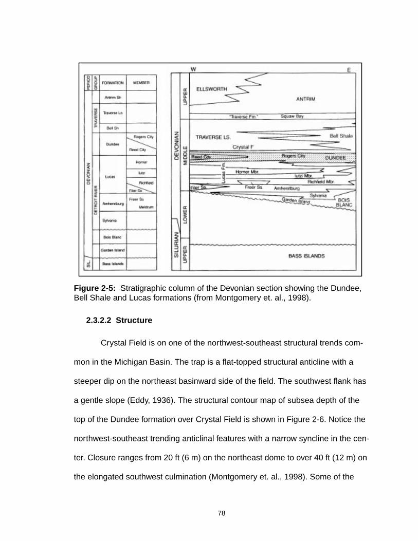
2.3.2.2 Structure
Crystal Field is on one of the northwest-southeast structural trends com-
mon in the Michigan Basin. The trap is a flat-topped structural anticline with a
steeper dip on the northeast basinward side of the field. The southwest flank has
a gentle slope (Eddy, 1936). The structural contour map of subsea depth of the
top of the Dundee formation over Crystal Field is shown in Figure 2-6. Notice the
northwest-southeast trending anticlinal features with a narrow syncline in the cen-
ter. Closure ranges from 20 ft (6 m) on the northeast dome to over 40 ft (12 m) on
the elongated southwest culmination (Montgomery et. al., 1998). Some of the
Figure 2-5: Stratigraphic column of the Devonian section showing the Dundee,Bell Shale and Lucas formations (from Montgomery et. al., 1998).
78

irregularity seen on the top Dundee surface may be due to karsting and solution
collapse. The presence of an erosional unconformity or disconformity at the top of
the Dundee surface is shown conclusively in most of the wells drilled (Eddy,
1936).
Trapping mechanisms in Crystal field are also related to stratigraphic fea-
tures. Off-structure wells are commonly wet, but have good porosity. The cap lime-
stone in these areas is also much thicker than in the areas of high structural relief
so most of the good reservoir rock is below the oil/water contact. Figure 2-7 is an
isopach map of the limestone cap at the top of the Dundee porosity. The lime-
stone cap is thinner along the anticlinal features.
Figure 2-6: Structure contour map of top subsea of the Dundee formation overCrystal Field, Michigan (Contour Interval = 7.5 ft). Location of the seismic lines areshown in red.
TOW 1-3
79

Figure 2-8 is a contour map of top subsea of the Dundee porosity zone
which is at the base of the limestone cap. The top of the Dundee porosity zone
also exhibits the same northwest-southeast trending anticlinal features as the top
of the Dundee formation. The highest point on the anticlinal structure in the
Dundee porosity zone should be the best place to explore for potential bypassed
reserves ("attic oil"). This, in conjunction with the limestone cap thickness should
help determine potential areas of interest.
Figure 2-7: Isopach map of the limestone cap at the top of the Dundee formationover Crystal Field, Michigan (Contour Interval = 5 ft).
TOW 1-3
80

The Bell Shale formation can provide a strong indication for the potential for
oil in the Dundee formation. Figure 2-9 is a contour map of subsea depth of the
top of the Bell Shale formation. The northwest-southeast trending features
present in the Dundee are also visible here. This formation was deposited either
during or following the karstification of the Dundee formation, and is expected to
be thicker in areas where karstification exists.
Due to the interlayering of limestone and shale in the Bell Shale formation,
the picks on the drillers’ logs may be questionable. They are sometimes inconsis-
Figure 2-8: Structure contour map of top subsea of the top of the Dundeeporosity over Crystal Field, Michigan (Contour Interval = 10 ft).
TOW 1-3
81

tent and all of the driller’s logs do not explain in detail the layers that were encoun-
tered. This probably degrades the contour and isopach maps.
Figure 2-10 is a isopach map of the Bell Shale formation. The thickness of
the shale increases to the northeast and southwest of the production area. The
most productive areas in Crystal Field correlate to a Bell Shale thickness of
approximately 50 feet or less, and the less productive area correlates to a thick-
ness of 60 feet or greater. The area of best production lies to the east of MOC
Line C-3 and between MOC Lines C-2 and C-5.
Figure 2-9: Structure contour map of top subsea of the Bell Shale formation overCrystal Field, Michigan (Contour Interval = 10 ft).
TOW 1-3
82

Figure 2-11 is a contour map of the initial production for the wells in the
field. The initial production rates in this field are as high as 5000 barrels of oil per
day. The higher initial production rates can be correlated to the anticlinal structure
for the Dundee and Dundee porosity, a small limestone cap thickness, and a
smaller thickness for the Bell Shale formation. The initial production rates are
somewhat useful but must be used with caution. During production of this field,
the wells were produced as quickly as possible and water coning occurred. This
may have an effect on the reliability of the results and the ability to use this data
for correlation purposes.
Figure 2-10: Isopach map of Bell Shale formation over Crystal Field, Michigan(Contour Interval = 10 ft).
TOW 1-3
83

Figure 2-12 shows a possible geologic model for the subsurface beneath
the TOW 1-3 well and the controls on by-passed oil production in Crystal Field.
The thickness of the limestone cap is small and the thickness of the Dundee
porosity zone is large compared to other non-productive areas in the field. The
Dundee porosity zone is also shallower where the TOW 1-3 well (horizontal leg)
was drilled compared to other areas around the well. This allows for a zone of
"attic" oil. This zone would still remain above the oil-water contact after water con-
ing or encroachment of water in the original reservoir. The thickness of the Bell
Shale was thick at the vertical well location of the TOW 1-3 well, apparently
Figure 2-11: Contour map of initial production in bbls/day of Crystal Field,Michigan (Contour Interval = 1000 bbls/day).
TOW 1-3
84

caused by a small karst featured observed in the core. Because of this, the verti-
cal well did not log the Dundee in the interval where the horizontal well (which
encountered porosity much higher) found production.
2.4 ProceduresThe data used for the contour and isopach maps are from well records and
drilling reports. These data were compiled by the Western Michigan University
Core Research Laboratory and Michigan Technological University. The contour
and isopach maps were created on a workstation using GeoQuest software.
The well log data was evaluated and cross-sections were created on a
workstation using GeoQuest software from Schlumberger GeoQuest. The seismic
data was interpreted poststack on a workstation using GeoQuest software. The
prestack data was processed by J. Haataja using iXL from Mercury International
Figure 2-12: Cross-section through Crystal Field showing the location andgeologic controls on production for the TOW 1-3 well (modified from Wood et. al,1998, Montgomery et. al., 1998, and Pennington, personal communication).
Bell Shalein Collapse
85

Technologies. A pseudo 3-D volume was created using offset for crosslines and
interpreted for amplitude variation with offset effects and is shown in Appendix B.
2.5 Results and Interpretation
2.5.1 Geophysical Well Log Interpretations
No cores or logs existed from Crystal Field prior to the drilling of the TOW
1-3 in 1995. The nearest wells with logs were located 2 to 5 miles away, and
include: 1) Shuttleworth #1 (Gratiot County), 2) Leonard Lee #1 (Montcalm
County), 3) Jennings-Smith #1-17 (Gratiot County), and 4) Chartreuse Rocha
Buck # 1-15 (Montcalm County). These wells are used to create general regional
cross-sections over the field area.
The top of the Bell Shale is identified by a significant increase in gamma
ray response, a slight decrease in resistivity, and a decrease in neutron porosity.
The Dundee - Bell Shale contact is marked by a distinct decrease in gamma-ray
values, an increase in resistivity, and an increase in neutron porosity in the upper
Dundee. The lower boundary with the Lucas formation is difficult to pick due to
lithologic similarity with the Dundee in the central Michigan basin. The Dundee-
Lucas contact has most often been chosen at the top of the shallowest anhydrite
bed (Montgomery, 1998).
Figure 2-13 is a basemap showing the location of the wells with logs and
seismic lines (MOC seismic lines and COCORP seismic lines) in the area around
the field. County names and Section, Township, and Range numbers are also
specified. Figure 2-14 and Figure 2-15 are cross-sections A-A’ and B-B’ which
show the Bell Shale and Dundee markers and the log response for the corre-
sponding formations. These figures are shown as measured depth so some of the
86

apparent structure is surface topography but they give the general structure over
the area.
Figure 2-16 is a Pickett plot, cross plotting the neutron porosity and resistiv-
ity well log responses, over the Dundee in order to determine the productivity of
the zone of interest. The TOW 1-3 is plotted along with four other wells (from the
Winterfield Field in Clare County) where well log data and production information
are available. The TOW 1-3 log data indicate water saturation values of approxi-
mately 50 percent. This leads to the interpretation that the TOW 1-3 well (vertical
leg) was drilled into a residual oil zone and that the horizontal kick-off tapped an
attic oil zone in the uppermost Dundee porosity above the section logged in the
vertical leg. The Thayer 3-29 well was drilled into a tight limestone in the upper
Dundee interval and has a water saturation between 50 and 75 percent.
Figure 2-13: Basemap showing the location of the seismic lines and cross-sections over Crystal Field, Michigan.
87
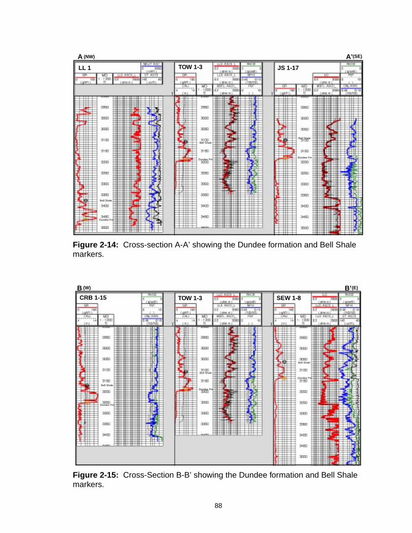
Figure 2-14: Cross-section A-A’ showing the Dundee formation and Bell Shalemarkers.
Figure 2-15: Cross-Section B-B’ showing the Dundee formation and Bell Shalemarkers.
(SE)
LL 1 TOW 1-3 JS 1-17
A A’(NW)
Bell Shale
Bell Shale
Bell Shale
Dundee Fm
Dundee FmDundee Fm
(E)
CRB 1-15 TOW 1-3 SEW 1-8
B B’(W)
Bell Shale
Dundee Fm
Bell Shale
Dundee Fm
Bell Shale
Dundee Fm
88

The Marion 33-21-1 and Austin 3-31 wells have an approximate water saturation
of 20 and 30 percent, respectively. This represents by-passed and some attic oil
present in the wells. The Johnson 4-31 well was drilled into a residual oil zone and
has a water saturation of 50 percent (with some attic oil present).
Figure 2-17 and Figure 2-18 show the log responses of the Thayer 3-29,
Johnson 4-31, Austin 3-31, and Marion 33-21-1 wells (from Winterfield Field)
compared to the TOW 1-3 well in Crystal Field. The Thayer 3-29 well has a similar
resistivity response but consists of tight limestone in the upper Dundee. The
Johnson 4-31 also shows a similar resistivity response to the TOW 1-3, and is
Figure 2-16: Pickett plot to show how the neutron porosity and resistivityresponses can be used to evaluate wells for wet or residual oil zones.
89
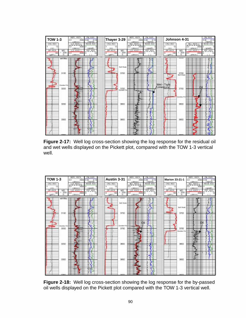
Figure 2-17: Well log cross-section showing the log response for the residual oiland wet wells displayed on the Pickett plot, compared with the TOW 1-3 verticalwell.
Figure 2-18: Well log cross-section showing the log response for the by-passedoil wells displayed on the Pickett plot compared with the TOW 1-3 vertical well.
TOW 1-3 Thayer 3-29 Johnson 4-31
Dundee Fm
Bell Shale
Dundee Fm
Bell Shale
Dundee Fm
Bell Shale
Wet - TightLimestone Oil
TOW 1-3 Austin 3-31 Marion 33-21-1
Bell Shale
Dundee Fm
Bell Shale
Dundee Fm
Bell Shale
Dundee Fm
Oil Oil
90

water saturated except for a couple thin oil zones. The Austin 3-31 and Marion 33-
21-1 both have a much higher resistivity indicative of an increase in oil saturation
and decrease in water saturation. This comparison of well logs strongly suggest
that the vertical leg of the TOW 1-3 well was drilled (and logged) in a swept zone
of residual oil in the Dundee. The horizontal leg of the TOW 1-3 well encountered
porous Dundee at approximately 18 feet higher, offset from the vertical well by
500 feet. Clearly the horizontal well was drilled into a zone of unproduced attic oil
at a high position in the reservoir.
2.5.2 Seismic Data Interpretations
Four poststack 2-D seismic lines, made available by Marathon Oil Com-
pany, are used to evaluate the application of seismic attributes for reservoir char-
acterization in Crystal Field. This study focuses on MOC Line C-3 because it is
located over the most productive part of the field and prestack data is available for
detailed studies and reprocessing.
This MOC seismic data used in this study was originally acquired to evalu-
ate potential for deeper horizons in and near Crystal Field. Due to the acquisition
parameters, the shallow seismic data (the Dundee is located at approximately
0.54 seconds) has low fold and short offsets, causing limited usefulness for seis-
mic attributes. The physical geography and water systems also have an effect on
seismic data. Many traces are missing from this data because of the presence of
lakes, swamps, and other obstacles that the acquisition team had to shoot around.
A significant glacial drift present in this area also causes statics problems in seis-
mic data acquisition and processing.
91

Figure 2-19 is a map of the field area showing the wells, in blue, and the
four 2-D seismic lines, in varying colors, where the two-way travel time for the
Dundee formation has been interpreted. Purple or green represents a larger two
way travel time, implying that the formation is deeper, and yellow and red indicate
higher time structures.
Figure 2-20 is a map of the field area showing the wells and the four 2-D
seismic lines where the amplitude of the seismic reflection at the Dundee forma-
tion is displayed. Green or purple represents where the amplitude is lower along
the seismic lines, and yellow and red indicate larger amplitudes. The location of
the TOW 1-3 well is specified.
Figure 2-21 is a three dimensional display of the MOC seismic lines in
Crystal Field. This display shows the orientation of the seismic lines and the entire
vertical time. MOC Line C-3 is the seismic line this study will focus on.
Figure 2-22 is MOC Line C-3 showing interpreted horizons of the Traverse
Limestone, Dundee formation, Salina formation, and C-Shale. The Dundee is the
horizon of interest and is located at approximately 0.54 seconds. The other inter-
secting seismic lines are shown as a red vertical line. The study area of Crystal
Field is located along MOC Line C-3 and between MOC Lines C-2 and C-5; it is
indicated on each figure.
Figure 2-23 shows the instantaneous phase along MOC Line C-3. The
Dundee formation is located at approximately 0.54 seconds and has a continuous
phase across the entire study area. The phase was important when correlating
the horizons due to the discontinuous nature of the reflection character.
92

Figure 2-19: Two-way travel time for the Dundee formation.
Figure 2-20: Amplitude variation of Dundee formation.
TOW 1-3
TOW 1-3
93

Figure 2-24 shows the reflection character along MOC Line C-3 in the
study area. Note the discontinuous nature of the reflection character along the
Dundee (0.54 seconds). This may be due to the low fold of the seismic data and/
or the karstification at the Bell Shale - Dundee boundary. Karstification causes
discontinuous reflections because of energy scattering and adsorption into the
highly porous surface, resulting in a low signal to noise ratio, and could be an indi-
cation of fracturing and porosity. High fold can help this problem because stacking
significantly reduces the noise and increases the signal to noise ratio. The glacial
till present in the area also causes problems with residual statics and increases
noise in the seismic data. A related study, reported in Appendix B, investigates the
pre-stack data of MOC Line C-3, and shows that, after mute, the CMP fold at the
Dundee was only six to eight traces.
Figure 2-25 shows the reflection character along MOC Line C_3 in the
study area after automatic gain control (AGC) has been applied. This improves
the appearance of the reflectors and enhances the Dundee formation but cannot
be used to determine the importance of seismic attributes, because AGC alters
the attributes such as amplitude.
Figure 2-26 is a three dimensional display of the seismic lines over Crystal
Field with the top subsea Dundee structure contour map imposed. The highest
area on the anticlinal structure is in red and represents the most productive part of
the field. This map was created using a basic time-depth relationship, knowing the
depth and time of the Dundee surface at certain points.
94

Figure 2-21: Three-dimensional display of MOC seismic lines in Crystal Field.
Figure 2-22: Line C-3 showing interpreted horizons on an amplitude display overthe study area.
MOC Line C-3
MOC Line C-2
MOC Line C-5
MO
C L
ine
C-4
Study Area
95
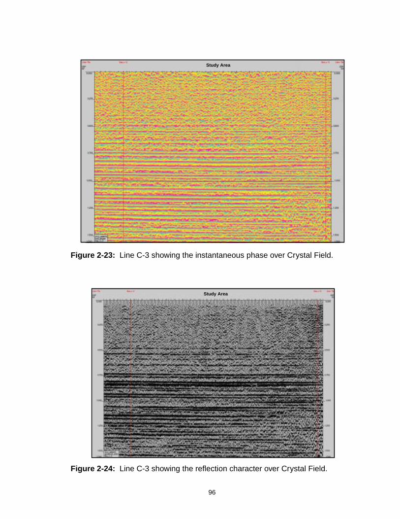
Figure 2-23: Line C-3 showing the instantaneous phase over Crystal Field.
Figure 2-24: Line C-3 showing the reflection character over Crystal Field.
Study Area
Study Area
96

Figure 2-25: Line C-3 showing the reflection character over Crystal Field afterautomatic gain control has been applied.
Figure 2-26: Three dimensional display of MOC seismic lines and top subseastructure contour of the Dundee formation.
Study Area
MOC Line C-3
MO
C Line C
-2
MOC Line C-4M
OC Line C-5
Dundee Structure ContourMap over Crystal Field
97

2.6 ConclusionsThe seismic data used in this study (MOC seismic lines) was initially
acquired to look for potential in deeper formations; because it was acquired for
deeper data, it had low values of fold and offset for the shallow data. This resulted
in difficulties relating seismic attributes to lithology and reservoir properties for
finding residual oil in shallow areas.
Data acquired for shallow horizons may be very useful for evaluating the
seismic attributes in other fields in the Michigan Basin if the fold and offset ranges
are appropriate. Good quality seismic data for the horizons of interest is neces-
sary to evaluate seismic attributes.
Poststack seismic attributes in MOC Line C-3, such as amplitude, are influ-
enced by the low fold and offset ranges in the seismic data (Appendix B) but
phase was consistent. Prestack seismic attributes are strongly dependent on fold
and offset ranges available in the dataset (Appendix B).
Residual statics are necessary and very important in processing to provide
a quality stack and good statics, especially in areas where glacial till is present.
Some of the noise and discontinuous reflections in the MOC seismic lines may be
due to statics problems.
The Bell Shale contour and isopach maps indicate that karstification is
present but the seismic data could not be used to support or disprove this due to
its poor quality in the shallow domain. The Bell Shale formation should be thicker
in areas where karstification has taken place. In Crystal Field, areas where the
Bell Shale is thinner tends to correlate with good initial production rates and a
smaller limestone cap.
98

2.7 Future WorkIn order to make seismic data useful checkshot and sonic logging data are
needed. It is crucial for seismic data analysis to acquire sonic logs and checkshot
data in newly drilled wells.
Perform 3-D visualization of the formation tops from the old wells and inte-
grate the well trajectories of the 3 new horizontal wells.
Perform advanced log interpretation techniques for fractured carbonates
where a, m, and n, vary in Archie’s equations.
Apply advanced refraction statics which may improve imaging of deeper
horizons in the existing seismic data.
If imaging is improved with refraction statics, successful attribute analysis
may be applied.
99

2.8 ReferencesAnnual statistical summary of oil and gas fields in Michigan 1935-1986: Michigan
Department of Natural Resources, Geological Survey Division, Lansing,MI.
Bassett, C.F., 1935, Stratigraphy and Paleontology of the Dundee Limestone ofSoutheaster Michigan: Bulletin of the Geological Society of America, Vol.46, p. 425-462.
Birchard, M.C., 1993, Stratigraphy and Facies of the Middle Devonian DundeeFormation: Ontario Geological Survey, Report # 5848.
Brown, L., Jensen, L., Oliver, S., Kaufman, S., and Steiner, D., 1982, Rift structurebeneath the Michigan Basin from COCORP profiling: Geology, Vol. 10, p.645-649.
Catacosinos, P.A., Daniels, Jr., P.A., and Harrison III, W.B., 1990, Structure,Stratigraphy and Petroleum Geology of the Michigan Basin: in Interior Cra-tonic Basins, AAPG Memoir 51: edited by Leighton, M.W. et. al., p 561-601.
Catacosinos, P.A., 1973, Cambrian Lithostratigraphy of Michigan Basin: AAPGBulletin, Vol, 57, No. 12, p. 2404-2418.
Chittick, S., 1995, Characterization of the Dundee Formation, Winterfield field,Clare County, Michigan: M.S. thesis, Michigan Technological University,Houghton, Michigan, 150p.
Curran, B.C., and Hurley, N.F., 1992, Geology of the Devonian Dundee Reservoir,West Branch Field, Michigan: AAPG Bulletin, Vol. 76, No. 9, p. 1363-1383.
Dorr, J.A., and Eschman, D.F., 1970, Geology of Michigan: The University of Mich-igan Press, Ann Arbor, MI, 476 pp.
Eddy, G.E., 1936, Geology of the Crystal Oil Field, Montcalm County, Michigan:Michigan Geological Survey, Progress Report #1, 8 pp.
Gardner, W.C., Middle Devonian stratigraphy and depositional environments in theMichigan basin: Michigan Basin Geological Society, Special Paper #1, 138pp.
Lilienthal, R.T., 1978, Stratigraphic Cross-Sections of the Michigan Basin: Michi-gan Geological Survey Report of Investigations, No. 19, 38 pp.
100

Michigan Department of Natural Resources, Geological Survey Division, OpenFile Records Correspondence, Operators Monthly Reports.
Montgomery, S.L., Wood, J.R., and Harrison III, W.B., 1998, Devonian DundeeFormation, Crystal Field, Michigan Basin: Recovery of Bypassed OilThrough Horizontal Drilling, AAPG Bulletin, Vol. 82, No. 8, 1445-1462.
Vogler, E.A., Meyers, P.A., and Moore, W.A., 1981, Comparison of Michigan BasinCrude Oils: Geochimica et Colmochimica Acta, Vol. 45, No. 11, p. 2287-2293.
Wilson, S.E., 1983, Small gas fields in Michigan: in The Future of small energyresources: an International conference, McGraw-Hill, New York, NY, p. 62-66.
Wines, H., 1997, Crystal Oil Field: M.S. thesis, Western Michigan University,Kalamazoo, Michigan, 112 p.
Wood, J.R., Pennington, W.D., and Harrison III, W.B., 1998, Recovery ofbypassed oil in the Dundee Formation (Devonian) of the Michigan Basinusing Horizontal Drains: Final Report Project DE-FC22-94BC14983,National Petroleum Technology Office, U.S. Department of Energy, 95 p.
Wood, J.R., Allen, J.R., Huntoon, J.E., Pennington, W.D., and Harrison III, W.B.,Taylor, E., Tester, C.J., 1996, Horizontal well taps bypassed Dundee oil inCrystal Field, Michigan: Oil and Gas Journal, Vol. 94, No. 43, p. 60-63.
Wood, J.R., Allen, J.R., Huntoon, J.E., Pennington, W.D., and Harrison III, W.B.,Taylor, E., Tester, C.J., 1996, Horizontal well success spurs more Devonianwork in Michigan: Oil and Gas Journal, Vol. 94, No. 44, p. 86-89.
101

APPENDIX A: Effects of Fluid Properties on Seismic Response
A.1 Figures from Chapter 1 in English (Oil Field) Units
Figure 1-7: Histogram showing the distribution of GOR for the samples in thestudy.
Figure 1-8: Plot showing the calculated live oil velocity (Batzle and Wang 1992Model) versus the laboratory live oil velocity (Batzle and Han 1997 Fluid Study).
Perfect Correlation
A-1

Figure 1-9: Plot of live and dead oil densities for the samples in the study and therelationship to GOR (the lines are a least squares regression through the datapoints).
Figure 1-10: Plot of the calculated velocity versus GOR for the samples in thestudy.
A-2

Figure 1-11: Plot of the calculated velocity versus API gravity for the samples inthe study.
Figure 1-12: Plot of calculated live oil modulus versus density for the samples inthe study.
A-3

Figure 1-13: Plot of calculated live oil velocity versus density for the samples inthe study.
Figure 1-14: Plot showing the calculated live oil velocity (Batzle and Wang 1992Model) and the laboratory live oil velocity (Batzle and Han 1997 Fluid Study)versus pressure for a sample in the study.
A-4
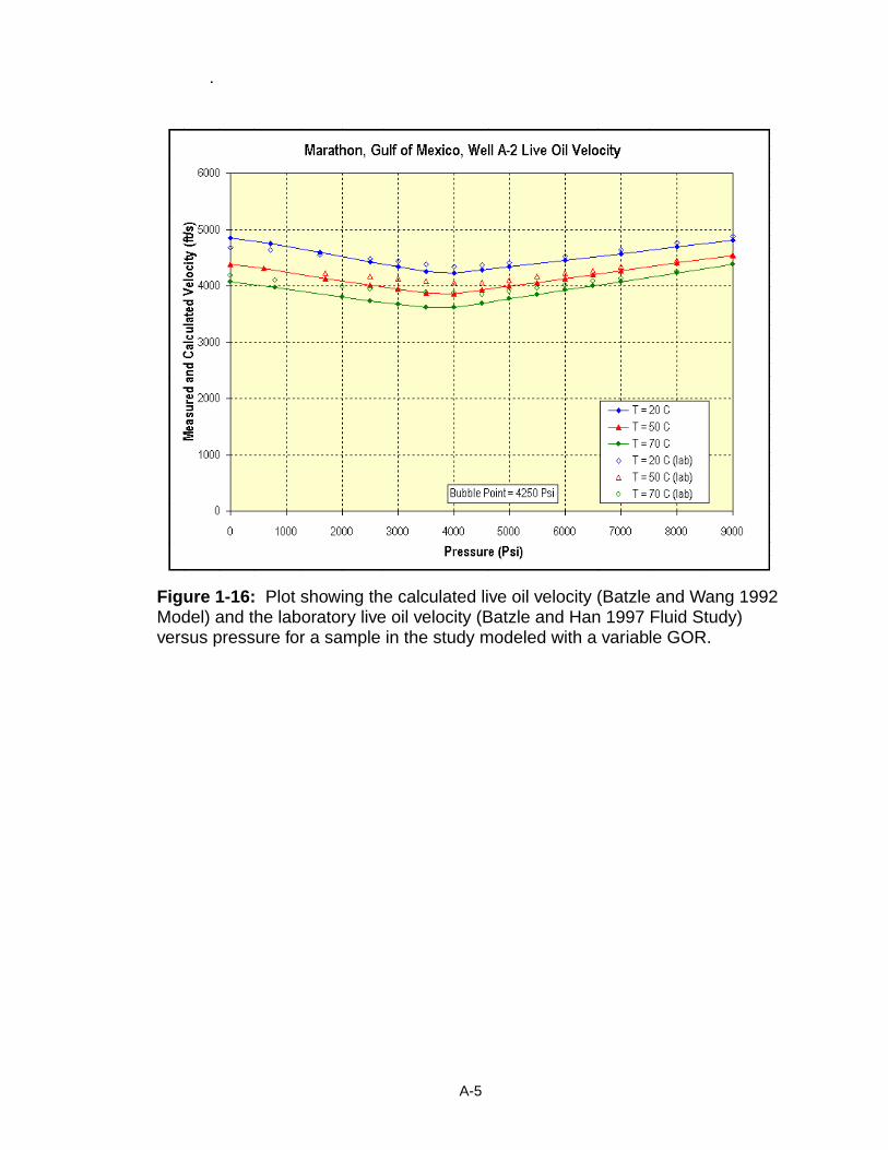
.
Figure 1-16: Plot showing the calculated live oil velocity (Batzle and Wang 1992Model) and the laboratory live oil velocity (Batzle and Han 1997 Fluid Study)versus pressure for a sample in the study modeled with a variable GOR.
A-5

Figure 1-20: Crossplot of fluid modulus and density as saturation values change.
X
A
A-6

Figure 1-22: A) Velocity versus saturation B) impedance and PR versussaturation showing how water saturation affects a two phase mixture of live oil andbrine in a sandstone matrix from water saturated to oil saturated conditions.
Figure 1-23: A) Impedance versus PR B) Percent change in impedance versuspercent change in PR showing how water saturation affects a two phase mixtureof live oil and brine in a sandstone matrix from water saturated to oil saturatedconditions.
A B
A
wet
depleted
conditionsreservoir
wet
depleted
conditionsreservoir
A B
wet
depleted
conditionsreservoir
A-7

Figure 1-24: Velocity versus density showing how water saturation affects a twophase mixture of live oil and brine in a sandstone matrix from water saturated tooil saturated conditions.
Figure 1-25: Compressional vs. shear velocity for a two phase mixture of live oiland brine in a sandstone matrix from water saturated to oil saturated conditions.
wet
depleted
reservoirconditions
wetdepleted
reservoirconditions
A-8

.
Figure 1-26: Fluid modulus versus pressure showing how the fluid moduluschanges as the pressure and saturation in the reservoir changes. Saturationvalues are shown as (% oil,% gas,% water).
A-9

.
Figure 1-27: Fluid density versus pressure showing how the density changes asthe pressure and saturation in the reservoir changes.Saturation values are shownas (% oil,% gas,% water).
A-10

Figure 1-28: Velocity and Poisson’s ratio versus pressure demonstrating thatwhen the reservoir drops below the bubble point (at 29.3 MPa) it significantlyeffects the reservoir properties. A) Modeled with a constant dry frame modulus.B) Modeled with a variable dry frame modulus with pressure.
A B
reservoirbubble conditionspoint
reservoirbubble
conditionspoint
A-11

A.2 Definition of Variables for the Batzle and Wang (1992) model
Input Constants/Conversions
T Temperature ρair Density of Air
P Pressure R Gas Constant
G Specific Gravity Ta Absolute Temperature
Rg Gas Oil Ratio ρo Oil Density
API API Gravity Dead Oil
S Weight Fraction NaCl Kd Dead Oil Modulus
Live Oil ρd Dead Oil Denisty
Kl Live Oil Modulus Vod Dead Oil Velocity
ρl Live Oil Density ρp Density at Pressure, P
Vol Live Oil Velocity (using Pseudoden- Gas
ρpl Density at Pressure, P Vg Gasl Velocity
ρgl Density at Gas Saturation Ks Adiabatic Gas Modulus
Bol Live Oil Gas Volume Factor ρg Gas Density
ρdl Pseudodensity based on gas expand γo Specific Gravity
Live Oil at Max GOR (δz/δPpr)T Gas deviation factor function pres-
Rgmax Maximum Live Oil Gas Oil Ratio Ppr Pseudoreduced Pressure
Klm Maximum Live Oil Modulus Tpr Pseudoreduced Temperature
ρlm Maximum Live Oil Density z Gas Deviation Factor
Volm Maximum Live Oil Velocity E Part of Gas Deviation Factor Equation
ρpm “Density at Pressure, P” Input (for mixtures)
ρgm Density at Gas Saturation Sg Gas Saturation
Bom Maximum Gas Volume Factor So Oil Saturation
ρpdm Pseudodensity based on gas expandi Sb Brine Saturation
Rgmax Maximum Live Oil Gas Oil Ratio, l/l Mixtures
Brine ρmd Dead Oil Mixture Density
Kgb Live Brine Modulus Kdo Dead Oil Mixture Modulus
Kb Dead Brine Modulus ρml Live Oil Mixture Density
Vb Brine Velocity Klo Live Oil Mixture Modulus
Vw Fresh Water Velocity ρmml Max Live Oil Mixture Density
ρw Fresh water Density Kmlo Max Live Oil Mixture Modulus
ρb Brine Density Vdo Dead Oil Mixture Velocity
log10 Rgb Log of Gas Water Ratio Vlo Live Oil Mixture Velocity
Rgb Gas Water Ratio Vmlo Max Live Oil Mixture Velocity
A-12

APPENDIX B: A Search for Seismic Attributes for Reservoir Char-acterization, Crystal Field, Michigan
B.1 Work that Josh Haataja did processing a 2-D seismic line (MOC Line C-3) in iXL.
Figure B-1 shows the flow chart used in iXL to reprocess MOC Line C-3
Figure B-1: Flow chart showing the processing sequence for MOC Line C-3.
B-1

and export the line as a pseudo 3-D seismic data set. Line C-3 was processed
through normal moveout.
Figure B-2 shows two bad common midpoint gathers for the 2-D seismic
line (MOC Line C-3). The low fold (12) and offset is obvious for these two common
midpoint gathers.
Figure B-2: Bad common midpoint gathers for MOC Line C-3.
B-2

Figure B-3 shows a better common midpoint gather where the fold (60) and
offset are much larger, but the fold and offset are still very low in the shallow
domain.
Figure B-4 and Figure B-5 are both common midpoint gathers that have
been imported into GeoQuest to evaluate amplitude variation with offset (AVO).
The headers of the seismic segy file were altered in iXL to allow CDP and offset to
be loaded as inline and crossline in GeoQuest. This resulted in a pseudo 3D seis-
mic display where amplitude is more readily interpreted. Due to the low fold and
offset a horizon could not be interpreted but this technique would be useful in
areas where better seismic data is available.
Figure B-3: Good common midpoint gather for MOC Line C-3.
B-3

Figure B-4: A common midpoint gather in GeoQuest showing AVO response.
Figure B-5: A common midpoint gather in GeoQuest showing AVO response.
B-4

Figure B-6: A time slice through the pseudo 3D volume at approximately 0.56seconds.
B-5

Figure B-6 is a time slice at approximately 0.56 seconds showing the
amplitude variation with offset (AVO) response.
Figure B-7 is a crossline where Line C-3 is shown at a specified offset. As
you can see a horizon along this line would be very difficult to interpret.
Figure B-7: Crossline showing MOC Line C-3 at a specified offset.
B-6

B.2 Formation Data Used to Create the Contour and Isopach Maps
B-7

B-8

B-9

B-10

B-11


